Chapter 2: Assessment of the Pacific cod stock in the Gulf of Alaska Steven Barbeaux, Kerim Aydin, Ben Fissel, Kirstin Holsman,

Ben Laurel, Wayne Palsson, Lauren Rogers, Kalei Shotwell,

Qiong Yang, and Stephani Zador

November 2019

Executive Summary

Summary of Changes in Assessment Inputs

Relative to last year’s assessment, the following changes have been made in the current assessment:

Changes in the input data

1. Federal and state catch data for 2018 were updated and preliminary federal and state catch data for

2019 were included;

2. Commercial federal and state fishery size composition data for 2018 were updated, and preliminary

commercial federal and state fishery size composition data for 2019 were included;

3. AFSC bottom trawl survey Pacific cod abundance index and length composition data for the GOA

for 2019 were included;

4. AFSC longline survey Pacific cod abundance index and length composition data for the GOA for

2019 were included;

5. Conditional length-at-age data for the 2010-2011 fisheries were added to the model.

Changes in the methodology

Model 18.10.44 is last year’s accepted model with the addition of the 2019 AFSC bottom trawl and longline

survey indices and length composition data, and fishery catch, length composition and age data including

conditional length-at-age data. There is one new data configuration and one new model explored this year

(see below).

Model configurations:

Model Data Plu

s gr

ou

p

Agi

ng

erro

r

Agi

ng

bia

s

18.10.44 No age data pre-2007 20+ No No

19.11.44 No age data pre-2007 10+ Yes No

19.14.48c All Cond. length at age 10+ Yes Pre-2007 fit, 2007+ fixed at 0

All proposed models presented for management were single sex age-based models with length-based

selectivity. The models have data from three fisheries (longline, pot, and combined trawl fisheries) with a

single season and two survey indices (post-1990 GOA bottom trawl survey and the AFSC Longline survey

indices). Length composition data were available for all three fisheries and both indices. Growth was

parameterized using the standard three parameter von Bertalanffy growth curve. Recruitment was

parameterized as a standard Beverton-Holt with steepness fixed at 1.0 and sigma R at 0.44. All selectivities

were fit using six parameter double-normal selectivity curves.

Model 18.10.44 performed well and is last year’s reference model, Model 19.11.44 is last year’s model

with this year’s data, a change to a 10+ age group instead of 20+, and the addition of aging error. Model

19.14.48c assumes aging bias in the pre-2007 age data. Kastelle et al. (2017) suggests only a limited

positive bias. This is best reflected in Model 19.14.48c and is therefore the Authors’ preferred model.

Model 19.14.48c results, like those of Model 18.10.44, includes a moderate increase in M for 2014-2016

and has a retrospective index within reasonable bounds for both spawning biomass and recruitment.

Summary of results

The data as interpreted through Model 19.14.48c indicates that the stock has been lower in abundance

than previously thought. It shows that the stock was likely below B20% since 2018 and will remain below

until 2021. Model 19.14.48c is nearly identical to last year’s model, the biggest influences in the model

were the drop in the AFSC longline survey index value and the lower than predicted value for the AFSC

trawl survey. Although the AFSC bottom trawl survey index value did increase, the increase was not as

high as last year’s model had predicted. To accommodate these new data the model estimated the

spawning biomass to have been lower than what was estimated last year relative to the unfished biomass.

This not only drove 2018-2019 to be below B20%, but also, despite an increasing trend, predicted that the

stock would remain below B20% in 2020. For 2020 the stock is estimated to be at B17.6%, above, but very

near the overfished determination level. The beginning of the year 2020 spawning biomass level is

projected to be the lowest of the time series and with the 2017 and 2018 year classes should see an

increase above B20% at the start of 2021.

Key results are tabulated below:

Quantity

As estimated or specified last

year for:

As estimated or specified this

year for:

2019 2020 2020 2021

M (natural mortality rate) 0.50 0.50 0.49 0.49

Tier 3b 3b 3b 3b

Projected total (age 0+) biomass (t) 207,198 266,066 203,373 261,484

Female spawning biomass (t)

Projected 34,701 34,774 32,958 42,026

B100% 172,240 172,240 187,780 187,780

B40% 68,896 68,896 75,112 75,112

B35% 60,284 60,284 65,723 65,723

FOFL 0.36 0.36 0.27 0.36

maxFABC 0.29 0.29 0.22 0.29

FABC 0.25 0.29 0.22 0.29

OFL (t) 23,669 26,078 17,794 30,099

maxABC (t) 19,665 21,592 14,621 24,820

ABC (t) *17,000 21,592 **14,621 **24,820

Status

2017 2018 2018 2019

Overfishing No n/a No n/a

Overfished n/a No n/a No

Approaching overfished n/a No n/a No

*Reduction from max to 17,000t to maintain stock above B20% in 2020 based on estimated end of year catch in 2018 of 13,096 t.

** Assumes 15,000 t catch in 2019 and no directed fishery in 2020 as reference level is below B20%. For 2021 projections the 2020 catch was

assumed to be 3,300 from state fisheries and 3,000 t from non-directed fishery bycatch.

Area apportionment

In 2012 the ABC for GOA Pacific cod was apportioned among regulatory areas using a Kalman filter

approach based on trawl survey biomass estimates. In the 2013 assessment, the random effects model

(which is similar to the Kalman filter approach, and was recommended in the Survey Average working

group report which was presented to the Plan Team in September 2013) was used; this method was used

for the ABC apportionment for 2014. The SSC concurred with this method in December 2013. Using this

method with the trawl survey biomass estimates through 2019, the area-apportioned ABCs are:

Western Central Eastern Total

Random effects area apportionment 22.7% 70.6% 6.7% 100%

2020 ABC 3,319 10,322 980 14,621

2021 ABC 5,634 17,523 1,663 24,820

It should be noted that for 2020 there would be no federal directed fishery allowed due to the stock

being below B20%. Catch was set at 3,300 t for state fishery and 3,000 t for bycatch in non-target

fisheries.

Responses to SSC and Plan Team Comments Specific to this Assessment

September 2019 Plan Team

The Team agrees with the author and recommends for the November meeting that models addressing

aging error, aging-bias, the 10+ age group, asymptotic selectivity for age, further explore whether

inclusion of the IPHC length composition data are appropriate (how many tows/sample sizes, etc.).

The model presented this year as the alternative (Model 19.14.48c) has all of these features. The IPHC

survey was not available until much too late to include in the assessment model this year. It will be

included in alternatives next year.

October 2019 SSC

In agreement with the author and the PT, the SSC would like to have models addressing aging bias and

error, a change to the maximum age bin, and asymptotic age selectivity be brought forward in November.

The model presented this year as the authors’ recommendation, Model 19.14.48c, includes all of these

features.

Introduction

Pacific cod (Gadus macrocephalus) is a transoceanic species, occurring at depths from shoreline to 500

m. The southern limit of the species’ distribution is about 34° N latitude, with a northern limit of about

63° N latitude. Pacific cod is distributed widely over Gulf of Alaska (GOA), as well as the eastern Bering

Sea (EBS) and the Aleutian Islands (AI) area. The Aleut word for Pacific cod, atxidax, literally translates

to “the fish that stops” (Betts et al. 2011). Recoveries from archeological middens on Sanak Island in the

Western GOA show a long history (at least 4500 years) of exploitation. Over this period, the

archeological record reveals fluctuations in Pacific cod size distribution which Betts et al. (2011) tie to

changes in abundance due to climate variability (Fig. 2.1). Over this long period colder climate conditions

appear to have consistently led to higher abundance with more small/young cod in the population and

warmer conditions to lower abundance with fewer small/young cod in the population.

Tagging studies (e.g., Shimada and Kimura 1994) have demonstrated significant migration both

within and between the EBS, AI, and GOA outside of spawning season (Fig. 2.2). There appears

to be substantial migration between the southern Bering Sea and the western GOA based on

tagging data, however little movement has been observed from the central GOA to the Western

GOA. Two recent genetics studies using Restriction-site Associated DNA sequencing have

indicated significant genetic differentiation among spawning stocks of Pacific cod in the Gulf of

Alaska and the Bering Sea (Drinan et al. 2018; Spies et al. 2019). The first study (Drinan et al.

2018) used 6,425 single-nucleotide polymorphism (SNP) loci to show high assignment success

>80% of five spawning populations of Pacific cod throughout their range off Alaska. Further

work using using 3,599 SNP loci and spawning samples throughout the range of Pacific cod off

Alaska, as well as a summer sample from the Northern Bering Sea in August 2017 showed

significant differentiation among all spawning groups (Spies et al. 2019). The three spawning

groups examined in the Gulf of Alaska, Hecate Strait, Kodiak Island, and Prince William Sound,

were all genetically distinct and could be assigned to their population of origin with 80-90%

accuracy (Fig. 2.3; Drinan et al. 2018). Cod that spawned at Unimak Pass in 2003 and 2018 were

genetically distinct from the Kodiak Sample (spawning year 2003), FST=0.004 and FST=0.001.

There was strong evidence for selective differentiation of some loci, including one that aligned to

the zona pellucida glycoprotein 3 (ZP3) in the Atlantic cod genome. This locus had the level of

differentiation of any locus examined (FST=0.071). ZP3 is known to undergo rapid selection

(Drinan et al. 2018), and completely distinct haplotypes have been observed in spawning cod

from Kodiak Island westward vs. Prince William Sound and samples to the east.

Although there appears to be some genetic differentiation within the GOA management area and

some cross migration between the Western GOA and southeastern Bering Sea the Pacific cod

stock in the GOA region is currently managed as a single stock. Further work is needed to

understand the genetic stock structure of cod in the GOA and its relationship with the Bering Sea

stock of cod during spawning and feeding periods.

Review of Early Life History

Pacific cod release all their eggs near the bottom in a single event during the late winter/ early spring

period in the Gulf of Alaska (Stark 2007). Unlike most cod species, Pacific cod eggs are negatively

buoyant and are semi-adhesive to the ocean bottom substrate during development (Alderdice and

Forrester 1971). Hatch timing/success is highly temperature-dependent (Laurel et al. 2008), with optimal

hatch survival occurring in waters ranging between 4-6°C (Bian et al. 2016) over a broad range of

salinities (Alderdice and Forrester 1971). Eggs hatch into 4 mm larvae in ~2 wks at 5°C (Laurel et al.

2008) and become surface oriented and available to pelagic ichthyoplankton nets during the spring (Doyle

and Mier 2016). During this period, Pacific cod larvae are feeding principally on eggs, nauplii and early

copepodite stages of copepod prey <300 um (Strasburger et al. 2014). Field observations show that larvae

achieve a larger size by late May in warm years compared to cooler years. Warm surface waters can

accelerate larval growth when prey are abundant (Hurst et al. 2010), while warm temperatures at depth

may shift the timing of spawning to earlier in the year as well as accelerate egg development, leading to

earlier timing of hatching. However, there is a negative correlation between temperature and abundance

of Pacific cod larvae in the Central and Western Gulf of Alaska (Doyle et al. 2009, Doyle and Mier

2016), suggesting that increased size does not translate into benefits for survival. Laboratory studies

suggest warm temperatures can indirectly impact Pacific cod larvae by way of two mechanisms: 1)

increased susceptibility to starvation when the timing and biomass of prey is ‘mis-matched’ under warm

spring conditions (Laurel et al. 2011), and 2) reduced growth by way of changes in the lipid/fatty acid

composition of the zooplankton assemblage (Copeman and Laurel 2010).

The spatial-temporal distribution of Pacific cod larvae shifts with ontogeny and is dependent on a number

of behavioral and oceanographic processes. In early April, Pacific cod larvae are most abundant around

Kodiak Island before concentrations shift downstream to the SW in the Shumagin Islands in May and

June (Doyle and Mier 2016). Newly hatched larvae are surface oriented and make extended diel vertical

migrations with increased size and development (Hurst et al. 2009). Larvae undergo a significant

developmental change (‘flexion’) between 10-15 mm and gradually become more competent swimmers

with increasing size (Voesenek et al. 2018). Very late stage larvae (aka ‘pelagic juveniles’) eventually

settle to the bottom in early July around 40 mm and use nearshore nurseries through the summer and early

fall in the Gulf of Alaska (Laurel et al. 2017).

Shallow, coastal nursery areas provide age-0 juvenile Pacific cod ideal conditions for rapid growth and

refuge from predators (Laurel et al. 2007). Settled juvenile cod associate with bottom habitats (e.g.,

macrophytes) and feed on small calanoid copepods, mysids, and gammarid amphipods during this period

(Abookire et al. 2007). At the end of August, age-0 cod become less associated with microhabitat features

and gradually move into deeper water in the fall (Laurel et al. 2009). Overwintering dynamics are

currently unknown for Pacific cod, although laboratory held age-0 juveniles are capable of growth and

survival at very low temperature (0°C) for extended periods (Laurel et al. 2016a)

Pelagic age-0 juvenile surveys of Pacific cod have been conducted in some years (Moss et al. 2016), but

they are prone to significant measurement error if they are conducted across the settlement period

(Mukhina et al. 2003). Therefore, 1st year assessments of Pacific cod in the Gulf of Alaska are better

suited during the early larval or later post-settled juvenile period. There are two surveys that routinely

survey early life stages of Pacific cod in the Gulf of Alaska during these phases: 1) the RACE EcoFOCI

ichthyoplankton survey in the western GOA (1979 – present, currently conducted during only odd-

numbered years; https://access.afsc.noaa.gov/ichthyo/index.php), and 2) the RACE FBE nearshore seine

survey in Kodiak (2006 – present). The EcoFOCI ichthyoplankton survey is focused in the vicinity of

Kodiak Island, Shelikof Strait and Shelikof Sea Valley and captures Pacific cod larvae primarily in May

when they are 5-8 mm in size (Fig. 2.4 and Fig. 2.5; Matarese et al. 2003). The Kodiak seine survey

occurs in two embayments and is focused on post-settled age-0 juveniles later in the year (mid-July to late

August) when fish are 40-100 mm in length (Laurel et al. 2016b). In 2018, Cooperative Research between

the AFSC and UAF spatially extended the Kodiak seine survey to include 14 different bays on Kodiak

Island, the Alaska Peninsula, and the Shumagin Islands (Fig 2.6; Litzow and Abookire 2018). In 2019 this

study was continued across nearly the same region at most of the original 2018 locations (13 bays, 72

seine sets).

The summer thermal conditions in the Central/Western GOA have historically been well-suited for high

growth and survival potential for juvenile Pacific cod (Laurel et al. 2017), but were likely sub-optimal

during the 2014-16 marine heatwave (Fig. 2.7 and Fig. 2.8). The Kodiak seine survey indicated that age-0

juvenile abundance was very low during this period. However, age-0 abundance returned to relatively

high numbers following a period of relative cooling in 2017 and 2018 (Fig 2.9). A strong 2018 age-0

cohort was also observed across the WGOA in the new Cooperative Research survey (Fig. 2.10). With the

warm conditions in 2019 both the surveys once again indicated very low abundance of the 2019 year

class. For perspective, 240 age-0 Pacific cod were captured in the Cooperative Research beach seine

survey this year, compared with 18,600 Pacific cod in 130 sets in 2018. The strong 2018 cohort was also

not evident in either of the 2019 beach seine surveys, although older juveniles may have shifted to cooler

depths beyond the gear. Ichthyoplankton surveys confirm the patterns observed in the beach seine

surveys, with the lowest and second-lowest larval abundance on record observed in 2015 and 2019

respectively.

The direct impacts of temperature on life history processes in Pacific cod are stage- and size-dependent

but these relationships generally are ‘dome shaped’ like other cod species (e.g., Hurst et al. 2010; Laurel

et al. 2016a). In the earliest stages (eggs, yolk-sac larvae), individuals have less flexibility to behaviorally

adapt and have finite energetic reserves (non-feeding), making them especially sensitive to changes in

thermal conditions. For instance, hatching success of Pacific cod eggs is temperature-dependent, and

drops rapidly as temperatures rise above ~6 °C. In most years, temperature does not appear to be a

limiting factor for eggs, but during the recent heatwave, bottom temperatures were above optimal for

successful hatching and may have reduced the reproductive potential of the stock (Lauren and Rogers, in

review). In later juvenile stages, individuals can move to more favorable thermal or food habitats that

better suit their metabolic demands. Changes in seasonal temperatures also influence how energy is

allocated. A recent laboratory study indicated age-0 juvenile Pacific cod shift more energy to lipid storage

than to growth as temperatures drop, possibly as a strategy to offset limited food access during the winter

(Copeman et al. 2017).

The AFSC will be investigating environmental regulation of 1st year of life processes in Pacific cod to

better understand the interrelationship between processes occurring during pre-settlement

(spawning/larvae), settlement (summer growth) and post-settlement (1st overwintering) phases. Transport

processes and connectivity between larval and juveniles nursery areas will continue to be an important

area of research as the Regional Oceanographic Model (ROMS) for the GOA is updated.

Fishery

General description

During the two decades prior to passage of the Magnuson Fishery Conservation and Management Act

(MFCMA) in 1976, the fishery for Pacific cod in the GOA was small, averaging around 3,000 t per year.

Most of the catch during this period was taken by the foreign fleet, whose catches of Pacific cod were

usually incidental to directed fisheries for other species. By 1976, catches had increased to 6,800 t.

Catches of Pacific cod since 1991 are shown in Table 2.2; catches prior to that are listed in Thompson et

al. (2011). Presently, the Pacific cod stock is exploited by a multiple-gear fishery, including trawl,

longline, pot, and jig components. Trawl gear took the largest share of the catch in every year but one from 1991-2002, although pot gear has taken the largest single-gear share of the catch in each year since

2003 (not counting 2017, for which data are not yet complete). Figure 2.11 shows landings by gear since

1977. Table 2.2 shows the catch by jurisdiction and gear type.

The history of acceptable biological catch (ABC) and total allowable catch (TAC) levels is summarized

and compared with the time series of aggregate commercial catches in Table 2.3. Changes in ABC over

time are typically attributable to three factors: 1) changes in resource abundance, 2) changes in

management strategy, and 3) changes in the stock assessment model. Assessments conducted prior to

1988 were based on survey biomass alone. From 1988-1993, the assessment was based on stock reduction

analysis (Kimura et al. 1984). From 1994-2004, the assessment was conducted using the Stock Synthesis

1 modeling software (Methot 1986, 1990) with length-based data. The assessment was migrated to Stock

Synthesis 2 (SS2) in 2005 (Methot 2005), at which time age-based data began to enter the assessment.

Several changes have been made to the model within the SS2 framework (renamed “Stock Synthesis,” or

SS3, in 2008) each year since then.

For the first year of management under the MFCMA (1977), the catch limit for GOA Pacific cod was

established at slightly less than the 1976 total reported landings. During the period 1978-1981, catch

limits varied between 34,800 and 70,000 t, settling at 60,000 t in 1982. Prior to 1981 these limits were

assigned for “fishing years” rather than calendar years. In 1981 the catch limit was raised temporarily to

70,000 t and the fishing year was extended until December 31 to allow for a smooth transition to

management based on calendar years, after which the catch limit returned to 60,000 t until 1986, when

ABC began to be set on an annual basis. From 1986 (the first year in which an ABC was set) through

1996, TAC averaged about 83% of ABC and catch averaged about 81% of TAC. In 8 of those 11 years,

TAC equaled ABC exactly. In 2 of those 11 years (1992 and 1996), catch exceeded TAC.

To understand the relationships between ABC, TAC, and catch for the period since 1997, it is important to understand that a substantial fishery for Pacific cod has been conducted during these years inside State

of Alaska waters, mostly in the Western and Central Regulatory Areas. To accommodate the State-

managed fishery, the Federal TAC was set well below ABC (15-25% lower) in each of those years. Thus,

although total (Federal plus State) catch has exceeded the Federal TAC in all but three years since 1997,

this is basically an artifact of the bi-jurisdictional nature of the fishery and is not evidence of overfishing

as this would require exceeding OFL. At no time since the separate State waters fishery began in 1997 has

total catch exceeded ABC, and total catch has never exceeded OFL.

Historically, the majority of the GOA catch has come from the Central regulatory area. To some extent

the distribution of effort within the GOA is driven by regulation, as catch limits within this region have

been apportioned by area throughout the history of management under the MFCMA. Changes in area-

specific allocation between years have usually been traceable to changes in biomass distributions

estimated by Alaska Fisheries Science Center trawl surveys or management responses to local concerns.

Currently the area-specific ABC allocation is derived from the random effects model (which is similar to

the Kalman filter approach). The complete history of allocation (in percentage terms) by regulatory area

within the GOA is shown in Table 2.4. Table 2.2 and Table 2.3 include discarded Pacific cod, estimated

retained and discarded amounts are shown in Table 2.5.

In addition to area allocations, GOA Pacific cod is also allocated on the basis of processor component

(inshore/offshore) and season. The inshore component is allocated 90% of the TAC and the remainder is

allocated to the offshore component. Within the Central and Western Regulatory Areas, 60% of each

component’s portion of the TAC is allocated to the A season (January 1 through June 10) and the

remainder is allocated to the B season (June 11 through December 31, although the B season directed

fishery does not open until September 1).

NMFS has also published the following rule to implement Amendment 83 to the GOA Groundfish FMP:

“Amendment 83 allocates the Pacific cod TAC in the Western and Central regulatory areas of the

GOA among various gear and operational sectors, and eliminates inshore and offshore allocations

in these two regulatory areas. These allocations apply to both annual and seasonal limits of

Pacific cod for the applicable sectors. These apportionments are discussed in detail in a

subsequent section of this rule. Amendment 83 is intended to reduce competition among sectors

and to support stability in the Pacific cod fishery. The final rule implementing Amendment 83

limits access to the Federal Pacific cod TAC fisheries prosecuted in State of Alaska (State) waters

adjacent to the Western and Central regulatory areas in the GOA, otherwise known as parallel

fisheries. Amendment 83 does not change the existing annual Pacific cod TAC allocation between the inshore and offshore processing components in the Eastern regulatory area of the

GOA.

“In the Central GOA, NMFS must allocate the Pacific cod TAC between vessels using jig gear,

catcher vessels (CVs) less than 50 feet (15.24 meters) length overall using hook-and-line gear,

CVs equal to or greater than 50 feet (15.24 meters) length overall using hook-and-line gear,

catcher/processors (C/Ps) using hook-and-line gear, CVs using trawl gear, C/Ps using trawl gear,

and vessels using pot gear. In the Western GOA, NMFS must allocate the Pacific cod TAC

between vessels using jig gear, CVs using hook-and-line gear, C/Ps using hook-and-line gear,

CVs using trawl gear, and vessels using pot gear. Table 3 lists the proposed amounts of these

seasonal allowances. For the Pacific cod sector splits and associated management measures to

become effective in the GOA at the beginning of the 2012 fishing year, NMFS published a final

rule (76 FR 74670, December 1, 2011) and will revise the final 2012 harvest specifications (76

FR 11111, March 1, 2011).”

“NMFS proposes to calculate of the 2012 and 2013 Pacific cod TAC allocations in the following

manner. First, the jig sector would receive 1.5 percent of the annual Pacific cod TAC in the

Western GOA and 1.0 percent of the annual Pacific cod TAC in the Central GOA, as required by

proposed § 679.20(c)(7). The jig sector annual allocation would further be apportioned between

the A (60 percent) and B (40 percent) seasons as required by § 679.20(a)(12)(i). Should the jig

sector harvest 90 percent or more of its allocation in a given area during the fishing year, then this

allocation would increase by one percent in the subsequent fishing year, up to six percent of the

annual TAC. NMFS proposes to allocate the remainder of the annual Pacific cod TAC based on

gear type, operation type, and vessel length overall in the Western and Central GOA seasonally as

required by proposed § 679.20(a)(12)(A) and (B).”

The longline and trawl fisheries are also associated with a Pacific halibut mortality limit which sometimes

constrains the magnitude and timing of harvests taken by these two gear types.

Recent fishery performance

Data for managing the Gulf of Alaska groundfish fisheries are collected in multiple ways. The primary

source of catch composition data in the federally managed fisheries for Pacific cod are collected by on-

board observers (Faunce et al. 2017). The Alaska Department of Fish and Game (ADFG) sample

individual deliveries for state managed fisheries (Nichols et al. 2015). Overall catch delivered is reported

through a (historically) paper and electronic catch reporting system. Total catch is estimated through a

blend of catch reporting, observer, and electronic monitoring data (Cahalan et al. 2014).

The distribution of directed cod fishing is distinct to gear type, Figure 2.12 shows the distribution of catch

from 1990-2015 for the three major gear types. Figure 2.13 and Figure 2.14 show the distribution of catch

for 2018 and 2019 through October 17, 2019 for the three major gear types. In the 1970’s and early to

mid-1980’s the majority of Pacific cod catch in the Gulf of Alaska was taken by foreign vessels using

longline. With the development of the domestic Gulf of Alaska trawl fleet in the late 1980’s trawl vessels

took an increasing share of Pacific cod and Pacific cod catch increased sharply to around 70,000 t

throughout the 1990’s. Although there had always been Pacific cod catch in crab pots, pots were first used

to catch a measurable amount of Pacific cod in 1987. This sector initially comprised only a small portion

of the catch, however by 1991 pots caught 14% of the total catch. Throughout the 1990s the share of the

Pacific cod caught by pots steadily increased to more than a third of the catch by 2002 (Table 2.2 and Fig.

2.11). The portion of catch caught by the pot sector steeply increased in 2003 with incoming Steller sea

lion regulations and halibut bycatch limiting trawl and by 2011 through 2019 the pot sector caught

approximately half the total catch of Pacific cod in the Gulf of Alaska.

In 2015 combined state and federal catch was 77,772 t (24%) below the ABC while in 2016 combined

catch was 64,071 t (35% below the ABC) and in 2017 catch was 48,734 t (45% below the ABC) (Table

2.3). The ABC was substantially reduced for 2018 to 18,000 t from 88,342 t in 2017, an 80% reduction.

This was a 65% reduction from the realized 2017 catch. In 2018 the total catch was 15,247 t. For 2019

the ABC was set below the maximum ABC at 17,000t and as of October 1, the 2019 combined fishery

has caught 13,373 t which is 79% of the ABC.

The largest component of incidental catch of other targeted groundfish species in the Pacific cod fisheries

by weight are skate species in combination followed by shark species, arrowtooth flounder, octopus, and

walleye pollock (Table 2.6). Rockfish, rock sole, and sculpin species also make up a major component of

the bycatch in these fisheries. Incidental catch of non-target species in the GOA Pacific cod fishery are

listed in Table 2.7.

Longline

For 1990-2015 the longline fishery had been dispersed across the Central and Western GOA, however

more longline catch taken to the west of Kodiak, with some longline fishing occurring in Barnabus trough

and a small concentration of sets along the Seward Peninsula (Fig. 2.12). The 2017 longline fishery was

predominantly conducted on the border of are 620 and 610 in deeper waters south of the Shumagin

Islands and South of Unimak Island to the western edge of the 610 GOA management area shelf. In 2018

and 2019 with the drastic cut in TAC the fishery showed very little effort the majority of catch being

south of the Shumagin Islands straddling the 610 and 620 management area edges (Fig. 2.13 and Fig.

2.14). The longline fishery tends to catch larger fish on average than the other fisheries (Fig. 2.15). The

mean size of Pacific cod caught in the longline fishery is 64 cm (annual mean varies from 58cm to 70cm).

There was a drop in the mean length of fish in the longline fishery between 1990 and 2010, however this

trend has been more variable over the last 10 years (Fig. 2.16). In the Central GOA the Longline fishery

the 2017 A season had a slower start than previous years, but eventually caught the A-season TAC by

mid-April; a point reached in 2016 three weeks earlier (Fig. 2.21). In 2018 and 2019 fewer boats

participated in the fishery and catch was substantially slower and lower than previous years. The A season

CPUE in the Central GOA longline fishery in 2018 was substantially lower than the previous years (Fig.

2.23) below 2008 catch rates when stock abundance had been at its previously lowest level. For both 2018

and 2019 the A- season longline fishery in the Western GOA appears to have started later than the

previous 4 years, effort was lower and CPUE in January through March of 2019 declined in the Western

GOA but was up in the Central GOA (Fig. 2.22, Fig. 2.24, and Fig. 2.25).

Pot

The pot fishery is a relatively recent development (Table 2.2) and predominately pursued using smaller

catcher vessels. In the Alaska state managed fishery an average of 84% of the state catch comes from pot

fishing vessels. In 2016 60% of the overall GOA Pacific cod catch was made using pots. Pot fishing

occurs close to the major ports of Kodiak, Sand Point and on either side of the Seward Peninsula (Fig.

2.12). In 2017 the observer coverage rate of pot fishing vessels was greatly reduced from 14% to ~4% this

impacts our ability to adequately identify the spatial distribution of the pot fishery. From the data

collected there appears to have been less fishing to the southwest of Kodiak in 2017, however this may be

due to low observer coverage. In 2018 and 2019 there were few observed hauls throughout the GOA (Fig.

2.13 and Fig. 2.14), this is likely due to the lower TAC and low fishing levels. The pot fishery in the

Central GOA moved to deeper water in 2017 through 2019 than previous years. The 2017 pot fishery in

both the Central and Western GOA showed a mark decrease in CPUE (Fig. 2.23) from 2016 and 2018

declined even further, however 2019 shows a marked increase in CPUE in both the Central and Western

GOA (Fig. 2.23).

The pot fishery generally catches fish greater than 40 cm (Fig. 2.17), but like the longline fishery there

was a declining trend in Pacific cod mean length in the fishery from 1998 through 2016 with the smallest

fish at less than 60cm on average caught during the 2016 fishery (Fig. 2.18). The 2017 through 2019

fishery data show a sharp increase in mean length, potentially due to a combination of the fishery moving

to deeper water and lower recruitment since 2014.

In 2017 the pot fishery in the Central GOA was slower than previous years and did not take the full TAC

for the A season. The 2017 pot fishery in the Western GOA appears to have been similar to 2016 (Fig.

2.22). In 2018 and 2019 the Pot fishery in both regions were slower than the previous three years. In the

Western GOA, approximately half the catch was caught in a single week in March. In 2018 CPUE during

the A season (January-April) in both the Central and Western GOA was lower than the previous three

years (Fig. 2.23), on par with CPUE during 2013 and 2008-2010 (Fig. 2.23). In January – March 2019

there was an increase in the pot fishery CPUE in both regions.

Trawl

The Gulf of Alaska Pacific cod trawl fishery rapidly developed starting in 1987, quickly surpassing the

catch from the foreign longline fishery pursued in the 1970’s to mid-1980s in 1987. The trawl fishery

dominated the catch into the mid-2000s, but was then replaced by increases in pot fishing in the mid-

2000’s. This transition to pot fishing was partially due to Steller sea lion regulations, halibut bycatch caps,

and development of an Alaska state managed fishery. The distribution of catch from the trawl fishery for

1990-2015 shows it has been widely distributed across the Central and Western GOA (Fig. 2.12) with the

highest concentration of catch coming from southeast of Kodiak Island in the Central GOA and around

the Shumigan Islands in the Western GOA. In 2016 trawl fishing in the Western GOA shows a shift away

from the Shumigan Islands further to the west around Sanak Island and near the Alaska Peninsula, this

continued through 2017. Trawl fishing in 2018 for the A season shows a similar pattern as 2017 with

large catches from around Sanak Island, but some increased effort on Portlock Banks to the southeast of

Kodiak. There was substantially less catch and observed effort in 2018 and 2019 (Fig. 2.13 and Fig. 2.14)

than previous years.

The trawl fishery catches smaller fish than the other two gear types with fish as small as 10 cm appearing

in the observed length composition samples (Fig. 2.19). The average size of Pacific cod caught by trawl in

the 1980’s was on average smaller than those caught later (Fig. 2.20). The trawl fishery shows an increase

in average size in the 1990s with the maturation of the domestic fishery. The decline in the mean length

from the mid-1990s until 2015 mimics that observed in the longline and pot fisheries with some

prominent outliers (2005-2006). The years 2005 and 2006 shows little observed fishing in the B-season

when smaller fish are more often encountered with this gear type. The mean size shows a sharp increase

in 2016 through 2019. The change to deeper depth and a larger proportion of the catch coming from the

Western GOA might partially explain this recent increase.

The 2018-2019 directed A-season trawl fishery in the Central GOA started much later than previous

years, catch rates were lower and the fishery did not take the full TAC (Fig. 2.21). Prior to 2018 the mean

CPUE for Pacific cod in both the Central and Western GOA had been stable to increasing over the

previous 10 years (Fig. 2.23). In 2018 there was no observed effort in the Central GOA. In the western

GOA there was very little observed effort, however where observed CPUE remained near 2017 levels. In

2019 there was little observed effort, however the effort observed showed a decrease in CPUE in both

regions from 2018.

Other gear types, non-directed, and non-commercial catch

There is a small jig fishery for Pacific cod in the GOA, this is a primarily state managed fishery and there

is no observer data documenting distribution. This fishery has taken on average 2,400 t per year. In 2017

through 2019 the jig fishery has remained low with catch at less than 500 t for all regions.

Pacific cod is also caught as bycatch in other commercial fisheries. Although historically the shallow

water flatfish fishery caught the most Pacific cod, since 2014 Pacific cod bycatch in the Arrowtooth

flounder target fishery has surpassed it (Table 2.8). The weight of Pacific cod catch summed for all other

target fisheries was 3,239 t in 2016, 2,726 in 2017, 2,786 in 2018, and as of October 1 2,682 t in 2019.

This following an all-time high of 10,780 t in 2015 with 1/3 of this from the Arrowtooth flounder target

fishery.

Non-commercial catch of Pacific cod in the Gulf of Alaska is considered to be relatively small at less than

400 t; data are available through 2017 (Table 2.9). The largest component of this catch comes from the

recreational fishery, generally taking approximately one-half of the accounted for non-commercial catch.

Other fishery related indices for stock health

There is a long history of evaluating the health of a stock by its condition which examines changes in the

weight to length relationship (Nash et al. 2006). Condition is measured in this document as the deviance

from a log linear regression on weight by length for all Pacific cod fishery A season (January-April) data

for 1992-2019. There is some variability in the length to weight relationships between Pacific cod

captured in the Central and Western GOA fisheries and among gear types. However, there is a consistent

trend in both areas for Pacific cod captured using longline and pot gear in there being lower condition

during 2015-2016 (Fig. 2.24 -2.27). In 2018 and 2019 the condition of fish in both the Central and

Western GOA are mixed with differences in condition by gear and season. The Central GOA longline

fishery shows improving condition in January through April (Fig. 2.24), however in 2019 the condition of

Pacific cod returned to a poor condition. The Central GOA pot fishery shows improvement in 2018 in

January through April as well (Fig 2.25), but lack of data availability in May through September limit our

ability to evaluate condition. In the Western GOA longline fishery cod condition in 2019 returned to

average in January through April (Fig. 2.26), but again like in the Central GOA we see worse than

average condition in the summer fishery. The Western GOA pot fishery shows improved cod condition in

2017 and 2018 following the heatwave (Fig. 2.27), but then again in the winter of 2019 cod condition

once again drops to below average. There were not enough data in the summer of 2019 to evaluate

condition in the Western GOA pot fishery.

Incidental catch of Pacific cod in other targeted groundfish fisheries is provided in Table 2.8 and

noncommercial catch of Pacific cod are listed in Table 2.9.

Indices of fishery catch per unit effort (CPUE) can be informative to the health of a stock, however CPUE

in directed fisheries can be hyper-stable with CPUE remaining high even at low abundance (Walters

2003). This phenomenon is believed to have contributed to the decline of the Northern Atlantic cod

(Gadus morhua) on the eastern coast of Canada (Rose and Kulka 1999). Instead we show the occurrence

of Pacific cod in other directed fisheries. We examine two disparate fisheries to evaluate trends in

incidental catch of Pacific cod, the pelagic walleye pollock fishery and the bottom trawl shallow water

flatfish fishery. The occurrence of Pacific cod in the pelagic pollock fishery appears to be an index of

abundance that is particularly sensitive to 2 year old Pacific cod, which are thought to be more pelagic.

The shallow water flatfish fishery tracks a larger portion of the adult population of Pacific cod. For the

pollock fishery we track incidence of occurrence as proportion of hauls with cod (Fig. 2.28). In the

shallow water flatfish fishery, catch rates in tons of Pacific cod per ton of all species catch were examined

(Fig. 2.29). For the pollock fishery the 2017 value is the lowest in the series (2008-2019) with a slight

increase in 2018 and continued increase in 2019 in areas 610 and 620. For the shallow water flatfish

fishery, 2017 was the lowest value with a slight increase in 2018 and 2019. It should be noted that none of

these indices are controlled for gear, vessel, or fishing practice changes.

Surveys

Bottom trawl survey

The Alaska Fisheries Science Center (AFSC) has been conducting standardized bottom trawl surveys for

groundfish and crab in the Gulf of Alaska since 1984. From 1984-1997 these were conducted every third

year, and every two years between 1999 and 2019. Two or three commercial fishing vessels are

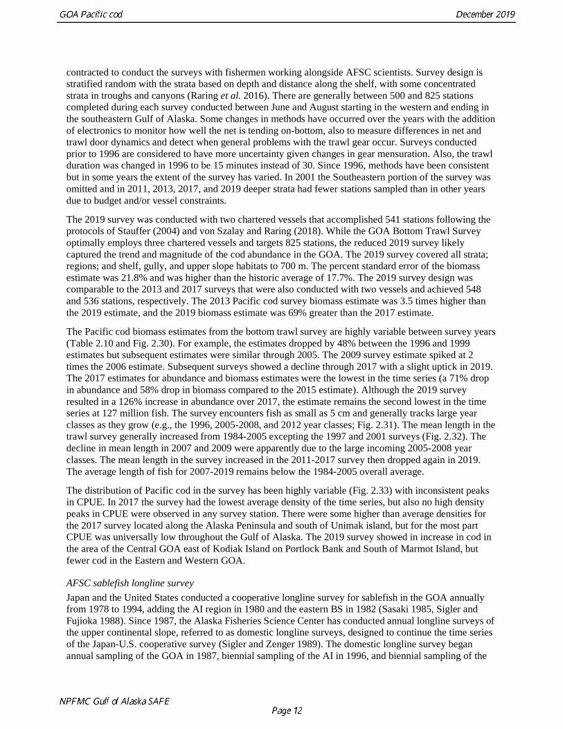
contracted to conduct the surveys with fishermen working alongside AFSC scientists. Survey design is

stratified random with the strata based on depth and distance along the shelf, with some concentrated

strata in troughs and canyons (Raring et al. 2016). There are generally between 500 and 825 stations

completed during each survey conducted between June and August starting in the western and ending in

the southeastern Gulf of Alaska. Some changes in methods have occurred over the years with the addition

of electronics to monitor how well the net is tending on-bottom, also to measure differences in net and

trawl door dynamics and detect when general problems with the trawl gear occur. Surveys conducted

prior to 1996 are considered to have more uncertainty given changes in gear mensuration. Also, the trawl

duration was changed in 1996 to be 15 minutes instead of 30. Since 1996, methods have been consistent

but in some years the extent of the survey has varied. In 2001 the Southeastern portion of the survey was

omitted and in 2011, 2013, 2017, and 2019 deeper strata had fewer stations sampled than in other years

due to budget and/or vessel constraints.

The 2019 survey was conducted with two chartered vessels that accomplished 541 stations following the

protocols of Stauffer (2004) and von Szalay and Raring (2018). While the GOA Bottom Trawl Survey

optimally employs three chartered vessels and targets 825 stations, the reduced 2019 survey likely

captured the trend and magnitude of the cod abundance in the GOA. The 2019 survey covered all strata;

regions; and shelf, gully, and upper slope habitats to 700 m. The percent standard error of the biomass

estimate was 21.8% and was higher than the historic average of 17.7%. The 2019 survey design was

comparable to the 2013 and 2017 surveys that were also conducted with two vessels and achieved 548

and 536 stations, respectively. The 2013 Pacific cod survey biomass estimate was 3.5 times higher than

the 2019 estimate, and the 2019 biomass estimate was 69% greater than the 2017 estimate.

The Pacific cod biomass estimates from the bottom trawl survey are highly variable between survey years

(Table 2.10 and Fig. 2.30). For example, the estimates dropped by 48% between the 1996 and 1999

estimates but subsequent estimates were similar through 2005. The 2009 survey estimate spiked at 2

times the 2006 estimate. Subsequent surveys showed a decline through 2017 with a slight uptick in 2019.

The 2017 estimates for abundance and biomass estimates were the lowest in the time series (a 71% drop

in abundance and 58% drop in biomass compared to the 2015 estimate). Although the 2019 survey

resulted in a 126% increase in abundance over 2017, the estimate remains the second lowest in the time

series at 127 million fish. The survey encounters fish as small as 5 cm and generally tracks large year

classes as they grow (e.g., the 1996, 2005-2008, and 2012 year classes; Fig. 2.31). The mean length in the

trawl survey generally increased from 1984-2005 excepting the 1997 and 2001 surveys (Fig. 2.32). The

decline in mean length in 2007 and 2009 were apparently due to the large incoming 2005-2008 year

classes. The mean length in the survey increased in the 2011-2017 survey then dropped again in 2019.

The average length of fish for 2007-2019 remains below the 1984-2005 overall average.

The distribution of Pacific cod in the survey has been highly variable (Fig. 2.33) with inconsistent peaks

in CPUE. In 2017 the survey had the lowest average density of the time series, but also no high density

peaks in CPUE were observed in any survey station. There were some higher than average densities for

the 2017 survey located along the Alaska Peninsula and south of Unimak island, but for the most part

CPUE was universally low throughout the Gulf of Alaska. The 2019 survey showed in increase in cod in

the area of the Central GOA east of Kodiak Island on Portlock Bank and South of Marmot Island, but

fewer cod in the Eastern and Western GOA.

AFSC sablefish longline survey

Japan and the United States conducted a cooperative longline survey for sablefish in the GOA annually

from 1978 to 1994, adding the AI region in 1980 and the eastern BS in 1982 (Sasaki 1985, Sigler and

Fujioka 1988). Since 1987, the Alaska Fisheries Science Center has conducted annual longline surveys of the upper continental slope, referred to as domestic longline surveys, designed to continue the time series

of the Japan-U.S. cooperative survey (Sigler and Zenger 1989). The domestic longline survey began

annual sampling of the GOA in 1987, biennial sampling of the AI in 1996, and biennial sampling of the

eastern BS in 1997 (Rutecki et al. 1997). The domestic survey also samples major gullies of the GOA in

addition to sampling the upper continental slope. The order in which areas are surveyed was changed in

1998 to reduce interactions between survey sampling and short, intense fisheries. Before 1998, the order

was AI and/or BS, Western Gulf, Central Gulf, Eastern Gulf. Starting in 1998, the Eastern Gulf area was

surveyed before the Central Gulf area. International Pacific halibut longline survey

A Relative Population Number (RPN) index of Pacific cod abundance and length compositions for 1990

through (Table 2.11 and Fig 2.34). Details about these data and a description of the methods for the AFSC

sablefish longline survey can be found in Hanselman et al. (2016) and Echave et al. (2012). This RPN

index follows the trend observed in the bottom trawl survey for 1990 through 2018 with a decline in

abundance from 1990 through 2008 and a sharp increase (154%) in 2009 and continued increase through

2011 with the maturation of the large 2005-2008 year classes. In 2012-2013 there appears a decline in the

abundance index concurrent with a drop in overall shelf temperature potentially due to changes in

availability of Pacific cod in these years as the population moved to shallower areas (Yang et al. 2019). In

2014-2016 the index increases but this may reflect increased availability with warmer conditions. The

index shows a sharp drop (53%) in abundance from 2016 to 2017, again (40%) from 2017 to 2018, and

yet again (37%) from 2018 to 2019. The 2019 estimate was 83% lower than the 2015 abundance estimate.

Unlike the bottom trawl survey, the longline survey encounters few small fish (Fig. 2.35). The size

composition data show consistent and steep unimodal distributions with a stepped decreasing trend in mean

size between 1990 and 2015 (Fig. 2.36) and then increasing mean size from 2015-2018 and a leveling off

in 2019. This matches the trend observed in all three fisheries. Changes in mean size appear consistent with

changing availability in the survey due to bottom temperatures and changes in the overall population with

large year classes. Smaller fish are encountered during this survey in warm years vs. cold years. There is a

sharp decline in mean size in 2009 when the large 2005 year-class would be becoming available to this

survey. The even steeper decline in average length in 2015 was encountered in the second warmest year on

record for the time series. In 2019 we would have expected both a more severe drop in average length due

to the increased temperatures on the shelf and an increase in abundance due to increased availability. That

we observed neither portends either very few small fish available in the population, or a change in behavior.

International Pacific halibut Commission (IPHC) longline survey

This survey differs from the AFSC longline survey in gear configuration and sampling design, but catches

substantial numbers of Pacific cod. More information on this survey can be found in Soderlund et al. (2009). A major difference between the two longline surveys is that the IPHC survey samples the shelf

consistently from ~ 10-500 meters, whereas the AFSC survey samples the slope and select gullies from

150-1000 meters. Because the majority of effort occurs on the shelf in shallower depths, the IPHC survey

may catch smaller and younger Pacific cod than the AFSC Longline survey. On the other hand, the IPHC

uses larger hooks (16/0 verus 13/0) than the AFSC longline survey which may prevent very small Pacific

cod from getting hooked. To compare, to IPHC relative population number’s (RPN) were calculated using

the same methods as the AFSC longline survey data (but using different depth strata). Stratum areas (km2)

from the RACE trawl surveys were used for IPHC RPN calculations. Length data on Gulf of Alaska

Pacific cod started being collected during this survey in 2018 although as of the writing of this document

(10/30/2019) the 2019 length data are not available.

The IPHC survey estimates of Pacific cod tracks well with both the AFSC sablefish longline and AFSC

bottom trawl surveys (Table 2.12 and Fig. 2.37). There was an apparent drop in abundance from 1997-

1999 with a stable but low population through to 2006. The population increases sharply starting in 2007,

likely with the incoming large 2005 year class and continues to increase through 2009 as the large 2005-

2008 year classes matured. The population then remained relatively stable through to 2014. The RPN index shows a steep decline in 2015 and 2017 consistent with the other two surveys. The 2017 RPN is the

lowest on record for the 20-year time series. This index shows a slight increase of the population

abundance in 2018 (28% from 2017) to values slightly higher than 2016, but remain the fourth lowest

estimate on record after 2001, 2016, and 2017. The 2019 survey again sees a slight increase above 2018

(8%), however the uncertainty in the estimate is high. The length composition data available from 2018

(Fig. 2.38) show the survey encounters fish greater than 40cm. The length data have a mode at

approximately 60 cm in the 610 management area. The other management areas have modes slightly

higher between 65 and 75 cm.

Alaska Department of Fish and Game bottom trawl survey

The Alaska Department of Fish and Game (ADFG) has conducted bottom trawl surveys of nearshore

areas of the Gulf of Alaska since 1987. Although these surveys are designed to monitor population trends

of Tanner crab and red king crab, Pacific cod and other fish are also sampled. Standardized survey

methods using a 400-mesh eastern trawl were employed from 1987 to the present. The survey is designed

to sample at fixed stations from mostly nearshore areas from Kodiak Island to Unimak Pass, and does not

cover the entire shelf area. The average number of tows completed during the survey is 360. On average,

89% of these tows contain Pacific cod. Details of the ADFG trawl gear and sampling procedures are in

Spalinger (2006).

To develop an index from these data, a simple delta GLM model was applied covering 1988-2018. Data

were filtered to exclude missing latitude and longitudes and missing depths. This model is separated into

two components: one that tracks presence-absence observations and a second that models factors

affecting positive observations. For both components, a fixed-effects model was selected and includes

year, geographic area, and depth as factors. Strata were defined according to ADFG district (Kodiak,

Chignik, South Peninsula) and depth (< 30 fathoms, 30-70 fathoms, > 70 fathoms). The error assumption

of presence-absence observations was assumed to be binomial but alternative error assumptions were

evaluated for the positive observations (lognormal versus gamma). The AIC statistic indicated the

lognormal distribution was more appropriate than the gamma (ΔAIC= 2068.99). Comparison of delta

GLM indices with the area-swept estimates indicated similar trends. Variances were based on a bootstrap

procedure, and CVs for the annual index values ranged from 0.06 to 0.14. These values underestimate

uncertainty relative to population trends since the area covered by the survey is a small percentage of the

GOA shelf area where Pacific cod have been observed.

The ADFG survey index follows the other three indices presented above with a drop in abundance

between 1998 and 1999 (-45%) and relatively low abundance throughout the 2000s (Table 2.13 and Fig.

2.39). This survey differs from other indices as the estimates only increased in 2012 (an 89% increase

from 2011), and then dropped off steadily afterwards to a record low in 2016. The 2017 survey index was

5% higher than the 2016 survey index. 2018 increased by 30% from 2017. The 2019 survey showed a

slight decline (15.7%) from 2018. Length composition data (Fig. 2.40) from this survey show wide multi-

modal length distributions are common with modes of age-0 fish at times available at near 10cm, however

the 2019 survey had no fish smaller than 22cm. The 2018 year class is apparent as a mode at between 29

cm and 36 cm and the 2017 year class at between 44 cm and 54 cm.

Environmental indices

CFSR bottom temperature indices

The Climate Forecast System Reanalysis (CFSR) is the latest version of the National Centers for

Environmental Prediction (NCEP) climate reanalysis. The oceanic component of CFSR includes the

Geophysical Fluid Dynamics Laboratory Modular Ocean Model version 4 (MOM4) with iterative sea-ice

(Saha et al. 2010). It uses 40 levels in the vertical with a 10-meter resolution from surface down to about

262 meters. The zonal resolution is 0.5° and a meridional resolution of 0.25° between 10°S and 10°N,

gradually increasing through the tropics until becoming fixed at 0.5° poleward of 30°S and 30°N.

To make the index, the CFSR reanalysis grid points were co-located with the AFSC bottom trawl survey

stations. The co-located CFSR oceanic temperature profiles were then linearly interpolated to obtain the

temperatures at the depths centers of gravity for 10 cm and 40 cm Pacific cod as determined from the

AFSC bottom trawl survey. All co-located grid points were then averaged to get the time series of CFSR

temperatures over the period of 1979-2019 (Fig. 2.41 and Table 2.14).

The mean depth of Pacific cod at 0 cm and 40cm was found to be 47.9 m and 103.4 m in the Central

GOA and 41.9 m and 64.07 m in the Western GOA. The temperatures of the 10 cm and 40 cm Pacific cod

in the CFSR indices are highly correlated (R2 = 0.88) with the larger fish in deeper and slightly colder

waters 7.49 °C vs. 6.00 °C in the Central GOA and 4.78 °C vs. 4.75 °C in the Western GOA. The

shallower index is more variable (CV10cm 0.10 vs. CV40cm=0.07). There are high peaks in water

temperature in 1981, 1987, 1998, 2015, 2016 and 2019 with 2019 being the highest in both the 10 cm and

40 cm indices. There are low valleys in temperature in 1982, 1989, 1995, 2002, 2009, 2012, and 2013.

The coldest temperature in the 10 cm index was in 2009 and in the 40 cm index in 2012. The trend is

insignificant for both indices.

Sum of annual marine heatwave cumulative intensity index (MHWCI)

The daily sea surface temperatures for 1981 through September 2019 were retrieved from the NOAA

High-resolution Blended Analysis Data database (NOAA 2017) and filtered to only include data from the

central Gulf of Alaska between 145°W and 160°W longitude for waters less than 300m in depth. The

overall daily mean sea surface temperature was then calculated for the entire region. These daily mean sea

surface temperatures data were processed through the R package heatwaveR (Schlegel and Smit 2018) to

obtain the marine heatwave cumulative intensity (MHWCI; Hobday et al. 2016) value where we defined a

heat wave as 5 days or more with daily mean sea surface temperatures greater than the 90th percentile of

the 1 January 1982 through 31 December 2012 time series. The MHWCI were then summed for each year

to create an annual index of MHWCI and summed for each year for the months of January through

March, November, and December to create an annual winter index of MHWCI.

The marine heatwave analysis using the daily mean Central GOA sea surface temperatures indicated a

prolonged period of increased temperatures in the Central GOA from 2 May 2014 to 13 January 2017

with heatwave conditions persisting for 815 of the 917 days in 14 events of greater than 5 days (Fig. 2.7).

The longest stretch of uninterrupted heatwave conditions occurred between 14 December 2015 and 13

January 2017 (397 days). By the criteria developed by Hobday et al. (2018) for marine heatwave

classification the event in the Central GOA reached a Category III (Severe) on 16 May 2016 with a peak

intensity (Imax) of 3.02°C. The heatwave had a summed cumulative intensity (Icum) for 2016 of

635.26°C days, more than 25% of the sum of the Icum for the entire time series (1981-2018). The 14

events of this prolonged heatwave period summed to 1291.91°C days or 52% of the summed Icum for the

time series.

There have been four periods of increased winter heatwave activity in the Central GOA, the first in 1983-

1986, second in 1997-2006, the third 2014-2016, and the fourth 2018-2019. Short winter marine

heatwaves (Category I to II) occurred every winter between 1983 and 1986, however none of these

exceeded 17 days and the total winter Icum for this period was 84.23°C days over a total of 86 days. In

the winter of 1997 there were two short (7 and 12 days) winter heatwave events with a total cumulative

intensity of 17.19 °C days. In 1998 there was a strong heatwave from 3 March to the 14 June (102 days)

with an Imax of 2.36°C and cumulative intensity of 146.01°C days. From 2001 through 2006 there were 6

winter heatwave events, most were minor and less than two weeks in length, however between 6

November 2002 and 4 March 2003 there were two that lasted in sum 141 days with a cumulative intensity

of 165.94°C days and an Imax of 2.04°C. The 2014-2016 series of marine heatwave as described above was substantially longer lasting and more intense than anything experience previously in the region. The

most recent heatwave began September 9, 2018 to the current date. There are six distinct events making

up the 2018-2019 heatwave with a maximum intensity of 2.75°C for the most recent heatwave period

from June 23, 2019 through September 10, 2019. The cumulative intensity of the 2018-2019 marine

heatwave is lower than the 2014-2016 heatwave, however the heatwave is still extant and may intensify.

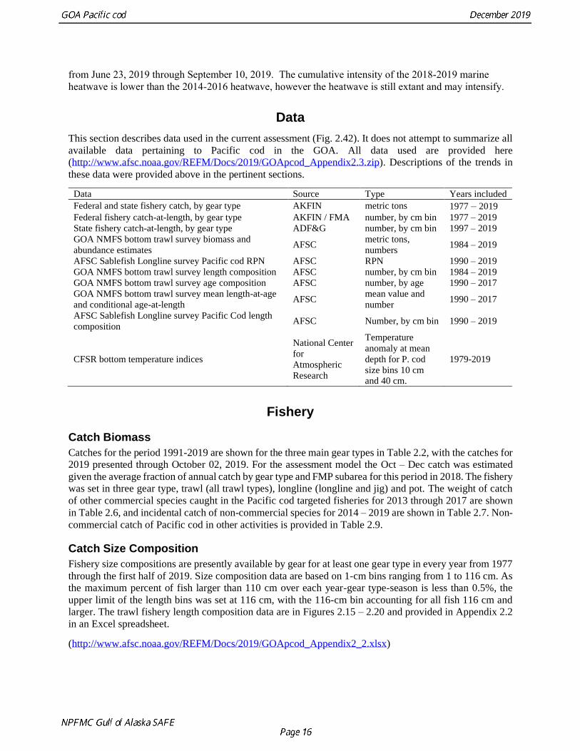
Data

This section describes data used in the current assessment (Fig. 2.42). It does not attempt to summarize all

available data pertaining to Pacific cod in the GOA. All data used are provided here

(http://www.afsc.noaa.gov/REFM/Docs/2019/GOApcod_Appendix2.3.zip). Descriptions of the trends in

these data were provided above in the pertinent sections.

Data Source Type Years included

Federal and state fishery catch, by gear type AKFIN metric tons 1977 – 2019

Federal fishery catch-at-length, by gear type AKFIN / FMA number, by cm bin 1977 – 2019

State fishery catch-at-length, by gear type ADF&G number, by cm bin 1997 – 2019

GOA NMFS bottom trawl survey biomass and

abundance estimates AFSC

metric tons,

numbers 1984 – 2019

AFSC Sablefish Longline survey Pacific cod RPN AFSC RPN 1990 – 2019

GOA NMFS bottom trawl survey length composition AFSC number, by cm bin 1984 – 2019

GOA NMFS bottom trawl survey age composition AFSC number, by age 1990 – 2017

GOA NMFS bottom trawl survey mean length-at-age

and conditional age-at-length AFSC

mean value and

number 1990 – 2017

AFSC Sablefish Longline survey Pacific Cod length

composition AFSC Number, by cm bin 1990 – 2019

CFSR bottom temperature indices

National Center

for

Atmospheric

Research

Temperature

anomaly at mean

depth for P. cod

size bins 10 cm and 40 cm.

1979-2019

Fishery

Catch Biomass

Catches for the period 1991-2019 are shown for the three main gear types in Table 2.2, with the catches for

2019 presented through October 02, 2019. For the assessment model the Oct – Dec catch was estimated

given the average fraction of annual catch by gear type and FMP subarea for this period in 2018. The fishery

was set in three gear type, trawl (all trawl types), longline (longline and jig) and pot. The weight of catch

of other commercial species caught in the Pacific cod targeted fisheries for 2013 through 2017 are shown

in Table 2.6, and incidental catch of non-commercial species for 2014 – 2019 are shown in Table 2.7. Non-

commercial catch of Pacific cod in other activities is provided in Table 2.9.

Catch Size Composition

Fishery size compositions are presently available by gear for at least one gear type in every year from 1977

through the first half of 2019. Size composition data are based on 1-cm bins ranging from 1 to 116 cm. As

the maximum percent of fish larger than 110 cm over each year-gear type-season is less than 0.5%, the

upper limit of the length bins was set at 116 cm, with the 116-cm bin accounting for all fish 116 cm and

larger. The trawl fishery length composition data are in Figures 2.15 – 2.20 and provided in Appendix 2.2

in an Excel spreadsheet.

(http://www.afsc.noaa.gov/REFM/Docs/2019/GOApcod_Appendix2_2.xlsx)

Size composition proportioning

For the 2016 assessment models fishery length composition data were estimated based on the extrapolated

number of fish in each haul for all hauls in a gear type for each year.

2016 Method: 𝑝𝑦𝑔𝑙 =∑

𝑛𝑦𝑔ℎ𝑙∑ 𝑛𝑦𝑎ℎ𝑙𝑙

𝑁𝑦𝑔ℎℎ

∑ 𝑁𝑦𝑔ℎ

Where p is the proportion of fish at length l for gear type g in year y, n is the number of fish measured in

haul h at length l from gear type g, and year y and N is the total extrapolated number of fish in haul h for

gear type g, and year y.

For 2017 through 2019 for post-1991 length composition we estimated the length compositions using the

total Catch Accounting System (CAS) derived total catch weight for each gear type, NMFS management

area, trimester, and year. Data prior to 1991 were unavailable at this resolution so those size composition

estimates are unchanged.

“New” method (post-1991): 𝑝𝑦𝑔𝑙 = ∑ ((∑

𝑛𝑦𝑡𝑎𝑔ℎ𝑙∑ 𝑛𝑦𝑡𝑎𝑔ℎ𝑙𝑙

𝑁𝑦𝑡𝑎𝑔ℎℎ

∑ 𝑁𝑦𝑡𝑎𝑔ℎ) (

𝑊𝑦𝑡𝑎𝑔

∑ 𝑊𝑦𝑡𝑎𝑔𝑡𝑎𝑔))𝑡,𝑎

Where p is the proportion of fish at length l for gear type g in year y, n is the number of fish measured in

haul h at length l from gear type g, NMFS area a, trimester t, and year y and N is the total extrapolated

number of fish in haul h for gear type g, NMFS area a, trimester t, and year y. The W terms come from the

CAS database and represent total (extrapolated) weight for gear type g, NMFS area a, trimester t, and

year y.

Addition of ADFG port sampling for Pot fishery data

In 2017 observer coverage changed as managers established electronic monitoring (EM) as a substitute

for observer coverage. This reduced observer coverage of the GOA Pacific cod pot fishery to ~4%

compared to 14.7% coverage in 2016 (Craig Faunce, personal comm. 25 July 2017). The EM program is

currently unable to measure fish for length composition (and obviously is unable to include age structure

sampling). In 2016 the pot fishery caught 59% of the total allocation of GOA Pacific cod with 75% of this

caught in state waters. This leaves a large proportion of the catch without observer collected length

composition data. To mitigate this loss of data, other sources of pot fishery length composition data are

being considered. The ADFG has routinely collected length data from Pacific cod landings since 1997. As

such, adding these data is a way to augment the pot fishery length composition data for the stock

assessment.

The ADFG port sampling and NMFS at-sea observer methods are follow different sampling frames so

combining them poses some challenges. We used ADF&G data from the pot fishery for trimester/areas in

which observer data were missing. The resolution of the ADF&G data required the assumption that all of

the samples collected in an area/trimester were representative of the overall catch for that trimester/area.

Method for ADFG data: 𝑝𝑦𝑡𝑎𝑔𝑙 =𝑛𝑦𝑔𝑙

∑ 𝑛𝑦𝑎𝑙𝑙(

𝑊𝑦𝑡𝑎𝑔

∑ 𝑊𝑦𝑡𝑎𝑔𝑡𝑎𝑔)

Where p is the proportion of fish at length l for gear type g in NMFS area a in trimester t for year y, n is

the number of fish measured at length l from gear type g in trimester t of year y. W is the catch accounting

total weight for gear type g, NMFS area a, trimester t, and year y.

Age composition

Otoliths for fishery age composition have been collected since 1982. In 2017, the Age and Growth

laboratory made a concerted effort to begin aging these data. These data have been processed in two

ways, the first was to develop an age and gear specific age-length key which was then used in conjunction

with the length composition data described above to create age composition distributions (Fig. 2.43). The

age data was also used to develop an annual conditional length-at-age matrix for each fishery (Fig. 2.44-

46).

Surveys

NMFS Gulf of Alaska Bottom Trawl Survey

Abundance Estimates

Bottom trawl survey estimates of total abundance used in the assessment models examined this year are

shown in Table 2.10 and Fig. 2.30, together with their respective coefficients of variation.

Length Composition

The relative length compositions used in the assessment models examined this year from 1984-2019 are

shown in Figure 2.47 and provided in Appendix 2.2 in an Excel spreadsheet

(http://www.afsc.noaa.gov/REFM/Docs/2019/GOApcod_Appendix2_2.xlsx).

Age Composition

Age compositions (Fig. 2.47) and conditional length at age (Fig. 2.48) from 1990-2017 trawl surveys are

available and included in this year’s assessment models. The age compositions and conditional length at

age data are provided in Appendix 2.2 in an Excel spreadsheet.

(http://www.afsc.noaa.gov/REFM/Docs/2019/GOApcod_Appendix2_2.xlsx)

Kastelle et al. (2017) state that one of the specific reasons for their study was to investigate the apparent

mismatch between the mean length at age (from growth-zone based ages) and length-frequency modal

sizes in the BSAI Pacific cod stock assessments and to evaluate whether age determination bias could

account for the mismatch. Mean lengths at age (either from raw age-length pairs or age-length keys) were

reported to be smaller than the modal size at presumed age from length distributions. In general, for the

specimens in their study, there was an increased probability of a positive bias in fish at ages 3 and 4

(Kastelle et al. 2017); that is, they were over-aged. In effect, this over-ageing created a bias in mean

length at age, resulting in smaller estimates of size at a given age. When correcting for ageing bias by

reallocating age-length samples in all specimens aged 2–5 in proportion to that seen in the true age

distribution, mean size at ages 2–4 did indeed increase (Kastelle et al. 2017). For example, there was an

increase of 35 mm and 50 mm for Pacific cod aged 3 and 4, respectively. This correction brings the mean

size at corrected age closer to modal sizes in the length compositions. While beyond the scope of their

study, they postulate that the use of this correction to adjust the mean size at age data currently included in Pacific cod stock assessments should prove beneficial for rectifying discrepancies between mean

length-at-age estimates and length-frequency modes.

To investigate aging bias the otoliths used in the seminal paper Stark (2007) were reread using the most

recent methods and reading criteria. There appeared to be a substantial change in the results to younger

fish at length for all collections used in the study. The length at age data were then plotted by year for

each age and a pattern appears where post-2007 fish at ages 2 through 6 were substantially larger than

those aged prior to 2007 (Fig. 2.49). Plotting all of the GOA AFSC bottom trawl survey age at length data

for 1996-2017 as pre- and post-2007 shows the bias is most apparent from ages 3 onward with at least one

year between length categories. Upon further investigation the apparent change in growth observed post-

2007 with fish becoming larger at age may have been due to a change in reading criteria and predominant

age readers. Aging bias for the pre-2007 ages were explored in this year’s proposed model configuration.

AFSC Longline Survey for the Gulf of Alaska

Relative Population Numbers Index and Length Composition

The AFSC longline survey for the Gulf of Alaska survey data on relative Pacific cod abundance together

with their respective coefficients of variation used in the assessment models examined this year are shown

in Table 2.12 and Fig. 2.34.

Length Composition

The length composition data for the AFSC longline survey data are shown in Figure 2.35 and provided in

Appendix 2.2 in an Excel spreadsheet.

(http://www.afsc.noaa.gov/REFM/Docs/2019/GOApcod_Appendix2_2.xlsx)

Environmental indices

CFSR bottom temperature indices

The CFSR bottom temperature indices for 10 cm Pacific cod were used in this assessment (see description

above; Table 2.14).

Analytic Approach

Model Structure

This year’s proposed model applies refinements to last year’s model in consideration of issues

encountered with aging error and aging bias discovered in the age data prior to 2007. To see the history of

models used in this assessment refer to A’mar and Palsson (2015). All models were run in Stock

Synthesis version 3.30.13.10 (Methot and Wetzell 2013). For consistency, we include the 2018 accepted

model (Model18.10.44) and the 2018 accepted model with updated data and a change in the age plus

group from 20+ to 10+.

All models presented were single sex, age-based models with length-based selectivity. The models have

data from three fisheries (longline, pot, and combined trawl fisheries) with a single season and two survey

indices (post-1990 GOA bottom trawl survey and the AFSC Longline survey indices). Length

composition data were available for all three fisheries and both survey indices. Conditional length at age

were available for the three fisheries and AFSC bottom trawl survey. Growth was parameterized using the

standard three parameter von Bertalanffy growth curve. Recruitment was modeled as varying about a

mean with standard deviation fixed at sigma R = 0.44 (Barbeaux et al. 2016). All selectivities were fit

using six parameter double-normal selectivity curves.

New models presented in this assessment were first reviewed by the NPFMC GOA Groundfish Plan

Team in September 2019 (this is provided in Appendix 2.1

http://www.afsc.noaa.gov/REFM/Docs/2019/GOApcod2019_Appendix2_1.pdf). All models presented in

consideration for use in management have been developed in SS v3.30. There is one new model series

explored this year (see below). All model configurations are shown below:

Model configurations:

Model Data Plu

s gr

ou

p

Agi

ng

erro

r

Agi

ng

bia

s

18.10.44 No age data pre-2007 20+ No No

19.11.44 No age data pre-2007 10+ Yes No

19.14.48c All Cond. length at age 10+ Yes Pre-2007 fit, 2007+ fixed at 0

Time varying selectivity components for all models:

Component Temporal Blocks/Devs

Longline Fishery Annually variable 1978-1989

Blocks – 1996-2004, 2005-2006, 2007-2016, 2017-2019 Trawl Fishery

Pot Fishery Blocks – 1977-2012 and 2013-2019

Bottom trawl survey Blocks – 1977-1995, 1996-2006, 2007-2019

All Stock synthesis files are provided in a zip file in Appendix 2.3:

(http://www.afsc.noaa.gov/REFM/Docs/2019/GOApcod2019_Appendix2.3.zip)

Parameters Estimated Outside the Assessment Model

Natural Mortality

In the 1993 BSAI Pacific cod assessment (Thompson and Methot 1993), the natural mortality rate M was

estimated to be 0.37. All subsequent assessments of the BSAI and GOA Pacific cod stocks (except the

1995 GOA assessment) have used this value for M, until the 2007 assessments, at which time the BSAI

assessment adopted a value of 0.34 and the GOA assessment adopted a value of 0.38. Both of these were

accepted by the respective Plan Teams and the SSC. The new values were based on Equation 7 of Jensen

(1996) and ages at 50% maturity reported by (Stark 2007; see “Maturity” subsection below). In response

to a request from the SSC, the 2008 BSAI assessment included further discussion and justification for

these values.

For the 2016 reference model (Model 16.08.25) M was estimated using a normal prior with a mean of

0.38 and CV of 0.1. In 2017 Dr. Thompson presented a new natural mortality prior based on a literature

search (Table 2.1) for the Bering Sea stock assessment (Thompson 2017). For the Gulf of Alaska stock,

we used the same methodology and literature search to devise a new prior for M. This resulted in a

lognormal prior on M of -0.81 (μ=0.44) with a standard deviation of 0.41 for the Gulf of Alaska Pacific

cod. All models presented were fit with this prior on M.

In 2017 it was hypothesized that due to the drop in all available survey indices between 2013 and 2017 it

was suspected that there was an increase in natural mortality during the height of the 2014-2016 natural

mortality. The 2017 reference model, Model 17.09.35 used a block for 2015-2016 where M could be fit

separately from all other years. In consideration of the marine heatwave analysis, models in 2018 expanded the natural mortality block to 2014-2016. For this Mstandard is fit separate from M2014-2016 with a

lognormal prior of μ=-0.81 and a σ of either 0.1 or 0.41. This configuration was used in the 2019

proposed models as well. The use of special mortality periods have been proposed and approved for use

in several Bering Sea crab assessments.

Growth

A three parameter von Bertalanffy growth model is used in the model. The growth parameters were set to

values based on a nonlinear least squares regression of the 2007-2015 AFSC GOA bottom trawl survey

length at age data (Fig. 2.50). The nls function form the nlstools library (Baty et al. 2015) in R was used

to fit the formula 𝐹𝐿 = 𝐿𝑖𝑛𝑓(1 − 𝑒(−𝐾(𝐴𝑔𝑒−𝑡0))) where FL is the fork length, Linf is the asymptotic

length, K is the growth rate, Age is the age of the fish, and t0 is the age where the fish had size 0. Variance

of the parameters were determined through bootstrap of the model with 1,000 iterations. Linf was

estimated at μ=99.46 CV=0.015, K was μ = 0.1966 CV=0.03, t0 was -0.11 CV=0.25.

Variability in Estimated Age

Variability in estimated age in SS is based on the standard deviation of estimated age. Weighted least

squares regression has been used in the past several assessments to estimate a linear relationship between

standard deviation and age. The regression was recomputed in 2011, yielding an estimated intercept of

0.023 and an estimated slope of 0.072 (i.e, the standard deviation of estimated age was modeled as 0.023

+ 0.072 × age), which gives a weighted R2 of 0.88. This regression was retained in the present assessment.

Weight at Length

Parameters governing the weight-at-length were estimated outside the model using AFSC GOA bottom

trawl survey data through 2015, giving the following values:

Value

: 5.63110−6

: 3.1306

Samples: 7,366

Maturity

A detailed history and evaluation of parameter values used to describe the maturity schedule for GOA

Pacific cod was presented in the 2005 assessment (Thompson and Dorn 2005). A length-based maturity

schedule was used for many years. The parameter values used for this schedule in the 2005 and 2006

assessments were set on the basis of a study by Stark (2007) at the following values: length at 50%

maturity = 50 cm and slope of linearized logistic equation = −0.222. However, in 2007, changes in SS

allowed for use of either a length-based or an age-based maturity schedule. Beginning with the 2007

assessment, the accepted model used an age-based schedule with intercept = 4.3 years and slope = −1.963

(Stark 2007). The use of an age-based rather than a length-based schedule follows a recommendation

from the maturity study’s author (James Stark, ret., Alaska Fisheries Science Center, personal

communication). The age-based parameters were retained through the 2017 assessment. The re-reading of

the Stark (2007) otoliths revealed that the parameters for maturity at age derived in this study are not

correct. It was therefore determined that management model should revert back to a length-based maturity

until the study can be reanalyzed. The decision to use length-based maturity was also made to

accommodate model options that will incorporate environmental effects on growth. The length at 50%

maturity was calculated using the morp_mature function in the sizeMat R package (Torrejon-Magallanes

2017) using all of the length at maturity data available from the Stark (2007) study for the Gulf of Alaska.

This included some maturity data that was not available to Stark (2007) at the time of publication and

some maturities from March and April not used in the calculation of L50% published. This resulted in the

following values: length at 50% maturity = 57.3 cm and slope of linearized logistic equation = -0.27365

(Fig. 2.51).

Aging Error

Aging error matrices were included in Models 19.11.44 and 19.14.48c (Fig. 2.52). These were developed

from age reader agreement testing results for otoliths read from the 2007-2017 bottom trawl surveys. The

standard deviation at age 3 was 0.57 and at age 10 was 1.16, the model assumed a linear interpolation

between these values and no error at ages 1 and 2.

Parameters Estimated Inside the Assessment Model

Parameters estimated conditionally (i.e., within individual SS runs, based on the data and the parameters

estimated independently) in the model include the von Bertalanffy growth parameters, annual recruitment

deviations, initial fishing mortality, gear-specific fishery selectivity parameters, aging bias adjustment

parameters, and survey selectivity parameters (Table 2.15).

The same functional form (pattern 24 for length-based selectivity) used in Stock Synthesis to define the

fishery selectivity schedules in previous year’s assessments was used this year for both the fishery and

survey. This functional form, the double normal, is constructed from two underlying and rescaled normal

distributions, with a horizontal line segment joining the two peaks. This form uses the following six

parameters (selectivity parameters are referenced by these numbers in several of the tables in this

assessment):

1. Beginning of peak region (where the curve first reaches a value of 1.0)

2. Width of peak region (where the curve first departs from a value of 1.0)

3. Ascending “width” (equal to twice the variance of the underlying normal distribution)

4. Descending width

5. Initial selectivity (at minimum length/age)

6. Final selectivity (at maximum length/age)

All but the “beginning of peak region” parameter are transformed: The widths are log-transformed and

the other parameters are logit-transformed.

In this year’s models both fishery and survey selectivities were length-based. Uniform prior distributions

were used for all selectivity parameters, except for dev vectors in models with annually varying

selectivities which were constrained by input standard deviations (“sigma”) of 0.2.

For all parameters estimated within individual SS runs, the estimator used was the mode of the logarithm

of the joint posterior distribution, which was in turn calculated as the sum of the logarithms of the

parameter-specific prior distributions and the logarithm of the likelihood function.

In addition to the above, the full set of year- and gear-specific fishing mortality rates were also estimated

conditionally, but not in the same sense as the above parameters. The fishing mortality rates are

determined exactly rather than estimated statistically because SS assumes that the input total catch data

are true values rather than estimates, so the fishing mortality rates can be computed algebraically given

the other parameter values and the input catch data.

For Model 19.14.48c aging bias was estimated for ages 3+ with two parameters, bias at age 3 and bias at

age 10, with a linear interpolation between the two, applied to all age data collected prior to 2007 (aged

prior to 2008). Age data from post 2007 were assumed to be aged without bias (Fig. 2.52).

Catchability

For all models the catchability for the AFSC bottom trawl survey was fit with a non-informative prior. All

prior. In all models presented this year, the AFSC longline survey catchability included a parameter, P,

which was used to additively adjust annual catchability values based on an annual temperature index, Iy,

as log(𝑄𝑦) = (�̅� + 𝑃𝐼𝑦) where Qy is catchability for a given year, and Q is the expected catchability

across all time. We used an index of mean annual temperature at depth for cod developed from the

Climate Forecast System Reanalysis (CFSR) as our temperature index (see description above). An

analysis introducing this methodology was presented in 2017 (Barbeaux et al. 2017) and a new method

validating this methodology was presented at the 2018 September Plan team meeting and provided in

Barbeaux et al. (2018) Appendix 2.1. It can be seen from the bottom trawl survey data below that the

centroid of distribution for Pacific cod greater than 34 cm shifts to deeper water in years with warmer

shelf temperatures. This relationship was verified in Yang et al. 2019 with a shift to deeper depths in all

size classes examined during warm years and shift to shallower waters in cold years. This shift would

make Pacific cod more available to the AFSC longline survey which starts at 150 m.

Figure: AFSC bottom trawl survey Pacific cod centroids of distribution for the Central GOA by shelf

temperature and Pacific cod size category. Dashed line shows starting depth of AFSC longline survey

(150 M).

Likelihood Components

The model includes likelihood components for trawl survey relative abundance, fishery and survey size

composition, survey age composition, survey mean size at age, recruitment, parameter deviations, and

“softbounds” (equivalent to an extremely weak prior distribution used to keep parameters from hitting

bounds), initial (equilibrium) catch, and survey mean size at age.

For all models presented there were no parameters near bounds and the likelihoods appear well defined

with the gradient of the objective function at less than 10e-4. All models were examined by “jittering”

starting parameters by 10% over 50 runs to evaluate if models had converged to local minima.

Use of Size and Age Composition Data in Parameter Estimation

Size and age composition data are assumed to be drawn from a multinomial distribution specific to a

particular year and gear within the year. In the parameter estimation process, SS weights a given size

composition observation (i.e., the size frequency distribution observed in a given year and gear) according

to the emphasis associated with the respective likelihood component and the sample size specified for the

multinomial distribution from which the data are assumed to be drawn. We set initial sample sizes for the

fishery at the number of hauls sampled or 200 whichever is least, for the surveys both size and age

composition sample sizes were initially set at 100.

Results

Model Evaluation

The 2018 final model with data from 2019, and new model configuration are presented. The new model

presented would be considered major model changes from the 2018 base model with ADSB values

greater than 0.1. Model evaluation criteria included AIC where applicable, model adherence to biological

principles and assumptions, the relative sizes of the likelihood components, and how well the model

estimates fit to the survey indices, the survey and fishery age composition and conditional age-at-length

data, reasonable curves for fishery and survey selectivity, and retrospective pattern. All models presented

adequately estimated the variance-covariance matrix. Model likelihoods and key parameter estimates are

provided in Table 2.16. Likelihoods by fleet are provided in Table 2.17. It should be noted that models

cannot be compared directly using likelihoods due to differences in data and aging error assumptions.

Retrospective results, index RMSE and composition mean effective sample sizes are provided in Table

2.18.

Comparing and Contrasting Model Configurations

The Model 18.10.44 was the same configuration as last year’s author’s preferred model and Model

19.11.44 was the same as that model with the addition of the 2019 data and a plus group at age 10 instead

of 20 and aging error. The Model 19.14.48c is the same as Model 19.11.44 except all conditional age at

length data are used and aging bias is fit for pre-2007 age data. The results from the GOA Pacific cod

stock assessment has been particularly volatile with a wide-array of models presented over the past 18

years (A’mar and Palsson 2015). The models presented this year are well within the bounds of models

presented in previous years for the spawning stock biomass time series (Fig. 2.53). The female spawning

biomass and age-0 recruitment for all the models considered this year are provided in Figure 2.54. All the

models show a similar fit, and similar recruitment and biomass trends. The size based selectivity (Fig.

2.55 and Fig. 2.56 are nearly indistinguishable among the three models. The difference between Model

18.10.44 and Model 19.14.48c comes down to the use of an age 10+ instead of 20+ maximum age,

application of aging error, the use of pre-2007 conditional age at length data, and fitted aging bias for the

pre-2007 data. There is no easy means of quantitatively comparing the two models. As expected the

introduction of aging error allows the model to have a slightly worse fit to the size composition and

conditional length at age data. None of the changes in fit are easily discernable by eye. Both models have

a similar fit to the indices. Model 19.11.44 provides a better fit to the survey indices. The slight

degredation of fit to both the length composition and the conditional age at length data is a result of

allowing aging error and placing slightly less emphasis on the composition data versus the indices.

Model 19.14.48c adds aging bias and the pre-2007 conditional age at length data. The additional

conditional age at length data causes a small change in fit to both survey indices (+0.39 LL) and the

length composition (+17.8 LL). There is little differences in fit among the three models except changes in

weighting of the different data components as more data are added and additional uncertainty is

quantified within the model.

Selection of Final Model

Comparing likelihoods or AIC was not appropriate for these models as there were changes in both data

and model error structure impacting weighting of data components. The retrospectives for Model

19.14.48c (Fig. 2.59) are marginally better than Model 18.10.44 (Table 2.18).

We recommend using Model 19.14.48c as the reference model for 2019 as the model allows for the use of

the pre-2007 age data using a temporally distinct aging bias and implements aging error as requested by

both the GOA Plan Team and SSC. This is a better treatment of uncertainty within the model. All Stock

Synthesis files for Model 19.14.48c are provided in a linked zip file here:

(http://www.afsc.noaa.gov/REFM/Docs/2018/GOApcod_Appendix2.3.zip).

Model 19.14.48c diagnostics and Suggestions for Future Improvement

Survey Indices

Model 19.14.48c fit to the NMFS bottom trawl survey was similar to previous base model fits (Fig. 2.55),

missing the 2009 bottom trawl survey estimate. Like previous models given the available length and age

composition data, the model was not able to increase abundance enough between 2007 and 2009 to match

the large increase in abundance between these two surveys and the model could also not fit the steepness

of the decrease in abundance between 2013 and 2017 and retain a good fit to the longline survey RPN

index which had a relatively high value for 2016. Comparison of total biomass predictions and AFSC

bottom trawl survey abundance estimates are relatively closely matched for the 1996-2017 values with

predictions at 1.07 times the survey estimates (Fig. 2.60), an effective “catchability” of 0.94.

Model 19.14.48c fits the AFSC longline index well (Fig. 2.57). The inclusion of the 10cm CFSR bottom

temperature index allowed the model to increase overall biomass in warm years and decrease it in cold

year, better fitting the spikes and valleys observed in the index as well as the overall decreasing trend

observed with the warming trend in the temperature index for 1990-2016. However the 2019 survey

estimate is not fit well, the index value was much lower than expected, the warmer temperatures should

have increased the availability of cod to the survey and the model was expecting a higher index. Given

that the mean size of fish also did not decrease with the warmer temperatures this indicates that either cod

did not become more available in 2019 due to warmer temperatures or there were few middle-aged fish

and the population is at a lower abundance than modeled.

Length Composition

Selectivities in Model 19.14.48c were not allowed to be dome-shaped, except for the pot fishery and

surveys (Fig. 2.61). Overall model predictions of the length compositions closely match the data for all

components (Fig. 2.62). For the trawl fishery the model predictions (Fig. 2.63 and Fig. 2.64) although

matching the mean length well, tended to underestimate the high peaks of the distributions and

overestimate either side of the peaks. The addition of the 2005-2006 block on the fit selectivity

parameters allowed the model to fit these two years well. Predictions of the longline fishery length

composition (Fig. 2.65 and Fig. 2.66) were well fit but similarly underestimated the high peaks of some of

the distributions, but matched the mean length very well. In addition, when the distributions tended to be

bimodal, the model tended to predict a single mode between the two modes. Predictions of the pot fishery

length composition (Fig. 2.67) were generally well fit, again, like the trawl and longline fisheries the high

peaks of the distributions tended to be underestimated. In addition the 2018 and 2019 fishery fits miss the

largest fish. This is likely due to the fishery moving to deeper waters and a change in selectivity that is not

accounted for in the model. The mean length for the pot fishery data were well matched for all years

except 2018 and 2019 where the mean was expected to be smaller. For the fishery length composition,

generally there is no need for improvement, residuals were small even for the minimal discrepancies

noted above for the peak modes. The authors will consider creating another block in the pot fishery for

2018 and 2019 for the 2020 assessment cycle.

Model 19.14.48c matched the NMFS bottom trawl survey length composition data mean lengths well

(Fig. 2.68), however like previous years small fish (sub-27 cm) the dominant length modes identified

were not always matched in magnitude. The sub-27 cm modes in 1996, 2007, and 2009 were estimated

lower than observed while a predicted mode for sub-27 cm fish in 2011 was not observed in the data. A

few peak modes were underestimated, but in general the larger fish were well predicted by the model.

Although the selectivity for Model 19.14.48c AFSC Longline survey length composition data (Fig. 2.69)

was not time varying, the predictions matched the data well. The 2008 and 2015 predictions were the only

ones that didn’t fit within the 95% confidence bounds of the mean length. For 2015 this was likely due to

smaller fish moving to deeper waters in this very warm year. For this survey in the future, fitting the

selectivity parameters on the CFSR temperature index, similar to how catchability is parameterized,

should be explored.

Age Composition and Length-at-Age

Even though the AFSC bottom trawl survey age composition data were not fit in the model and did not

contribute to the objective function we are able to examine how consistent the model expectations are to

the data (Fig. 2.70). The aging bias adjustment appears to have corrected the problem identified in

previous assessments with poor fits to the pre-2007 age composition data. The model expectations for age

composition are consistent with the data for all years except 1987.

Model 19.14.48c has time-invariant growth (Fig. 2.71). Fits to the conditional length-at-age data are

within the error bounds for most ages (Fig. 2.72, Fig. 2.73, Fig. 2.74, and Fig. 2.75), however there

appears to be some inter-annual variability that was not captured in this model. For instance, Pacific cod

in 2011 and 2015 AFSC bottom trawl survey were predicted in Model 19.14.48c to be larger at age than

the data shown for the oldest fish, while 2013 the opposite was true. The fishery data appear more

consistent, except for 2017 where the larger Pacific cod in both the longline and pot fisheries are

predicted to be older at size than the data suggests. This was not observed in the 2017 trawl survey data.

Fitting these data may be improved with annually varying growth, however reliable data for pre-2007 data

are not available, and therefore modeling inter-annual variability prior to 2007 may not be possible.

Mean length and weight at age from Model 19.14.48c are provided in Table 2.19.

Time Series Results

Definitions

The biomass estimates presented here will be defined in two ways: 1) total biomass was defined as age 0+

biomass, consisting of the biomass of all fish aged 0 years or greater in a given year; and 2) spawning

biomass was defined as the biomass of all spawning females in a given year. The recruitment estimates

presented here was defined as numbers of age-0 fish in a given year; actual recruitment to fishery and

survey depends on selectivities as estimated (noting that there are no indices involving age-0 Pacific cod).

All results presented are from Model 19.14.48c.

Biomass

Estimates of total biomass were on average 107% higher than the NMFS bottom trawl survey total

biomass estimates. Total biomass estimates show a long decline from their peak of 778,122 t in 1988

(Table 2.20 and Fig. 2.76) to 264,538 in 2006 and then an increase to another peak in 2014 of 498,565 t

then decrease continuously through 2018. With improved recruitment in 2017 and 2018 total biomass

began to increase again in 2019. Spawning biomass (Table 2.20) shows a similar trend of decline since

the late 1980s with a peak in 1990 at 248,915 t to a low in 2008 of 61,215 t. There was then a short

increase in spawning biomass coincident with the maturation of the 2005-2008 year classes through 2014

to 113,830 t, after which the decline continued to lowest level of 32,957 t projected for 2020. Projections

of Model 19.14.48c indicate that the stock has been below B20% since the beginning of the year 2018 and

will be projected to below B20% until the beginning of the year 2021.

Numbers at age and length are given in Appendix 2.2 and shown in Figure 2.95 and available online at:

(http://www.afsc.noaa.gov/REFM/Docs/2017/GOApcod2019_Appendix2.2.xlsx)

Recruitment and Numbers at Age

The recruitment predictions in Model 19.14.48c (Table 2.21, Fig. 2.78 and Fig. 2.79) show large 1977,

1980-1982,1984-1985, 1987,1989-1990, 2008, and 2011-2012 year-classes with more than 0.8 billion (at

age-0) fish for each, although uncertainty on the 1977 and 1984 year-class estimates were large (σ1977 =

0.37 and σ1984-1990 > 0.14). Between 1991 and 2010 the average recruitment was estimated at 0.492 billion,

40% lower than the 1977-1989 mean recruitment of 0.82 billion and 20% lower than the 1977-2017 mean

recruitment of 0.619 billion.

Fishing Mortality

Fishing mortality appears to have increased steadily with the decline in abundance from 1990 through a

peak in 2008 with continued high fishing mortality through 2017 in all models examined (Table 2.22). This

period saw both a decline in recruitment paired with increases in catch. The period of increasing fishing

mortality was mainly attributed to the rise in the pot fishery, which also shows the largest increase in

continuous F (Fig. 2.80). There is a steep rise in F in 2016 and 2017 following the sharp population drop

during the 2014-2016 marine heatwave. In 2018 and 2019 there was a sharp decrease in fishing mortality

coincident with the drastic cuts in ABC. The phase plane plot (Fig. 2. 81) shows that F was estimated to

retrospectively have been above the ABC control rule advised levels for 2005 through 2011 and 2015

through 2017 and biomass was below B35% in 2008 and 2009 and again 2016 through 2019, and projected

to continue to be below through 2021. The spawning biomass in 2018 through 2020 is projected to be below

B20%. It should be noted that this plot shows what the current model predicts, not what the past assessments

had estimated.

Retrospective analysis

Estimates of spawning biomass for Model 19.14.48c with an ending year of 2009 through 2019 are

consistently positively biased from 1984 through 2000, but have inconsistent bias post-2000 (Fig. 2.59).

The Mohn’s ρ for SSB ends up at 0.118, a Woods Hole ρ of 0.148 and an RMSE of 0.174 (Table 2.18).

All of the models examined this year had retrospective patterns within reasonable bounds.

MCMC results

MCMC were conducted with 1,000,000 iterations with 150,000 burn-in and thinned to every 1000th

iteration leaving 850 iterations for constructing the posterior distributions. Geweke (1992) and

Heidelberger and Welch (1983) MCMC convergence tests, as implemented in the coda R library

(Plummer et al. 2006), concluded adequate convergence in the chain (Fig. 2.82). Posterior distributions of

key parameters appear well defined and bracket the MLE estimates (Table 2.23). Using the projection

model estimate for unfished spawning biomass (187,780 t) then there is an 85.3% probability that the

stock was below B20% in 2019 and a 39.8% probability the stock was below B17.5% (Fig 2.83 and Fig.

2.84). For 2020 there is a 73.3% probability of the stock being below B20% and 27.7% probability of it

being below B17.5%.

Harvest Recommendations

Amendment 56 Reference Points

Amendment 56 to the GOA Groundfish Fishery Management Plan (FMP) defines the “overfishing level”

(OFL), the fishing mortality rate used to set OFL (FOFL), the maximum permissible ABC, and the fishing

mortality rate used to set the maximum permissible ABC. The fishing mortality rate used to set ABC

(FABC) may be less than this maximum permissible level, but not greater. Because reliable estimates of

reference points related to maximum sustainable yield (MSY) are currently not available but reliable

estimates of reference points related to spawning per recruit are available, Pacific cod in the GOA have

generally been managed under Tier 3 of Amendment 56. Tier 3 uses the following reference points: B40%,

equal to 40% of the equilibrium spawning biomass that would be obtained in the absence of fishing; F35%,

equal to the fishing mortality rate that reduces the equilibrium level of spawning per recruit to 35% of the

level that would be obtained in the absence of fishing; and F40%, equal to the fishing mortality rate that

reduces the equilibrium level of spawning per recruit to 40% of the level that would be obtained in the

absence of fishing. The following formulae apply under Tier 3:

3a) Stock status: B/B40% > 1

FOFL = F35%

FABC < F40%

3b) Stock status: 0.05 < B/B40% < 1

FOFL = F35% (B/B40% - 0.05) × 1/0.95

FABC < F40% (B/B40% - 0.05) × 1/0.95

3c) Stock status: B/B40% < 0.05

FOFL = 0

FABC = 0

Other useful biomass reference points which can be calculated using this assumption are B100% and B35%,

defined analogously to B40%. These reference points are estimated as follows, based on this year’s model,

Model 19.14.48c:

Reference point: B35% B40% B100%

Spawning biomass: 65,723t 75,112 t 187,780 t

For a stock exploited by multiple gear types, estimation of F35% and F40% requires an assumption

regarding the apportionment of fishing mortality among those gear types. For this assessment, the

apportionment was based on this year’s model’s estimates of fishing mortality by gear for the five most

recent complete years of data (2013-2018). The average fishing mortality rates implied that total fishing

mortality was divided among the three main gear types according to the following percentages: trawl

30%, longline 20%, and pot 50%. This apportionment of catch given the projected selectivity for each

gear results in estimates of F35% and F40% of 0.67 and 0.54 in aggregate.

Specification of OFL and Maximum Permissible ABC

Spawning biomass for 2020 is estimated by this year’s model to be 32,958 t at spawning. This is below

the B40% value of 75,112 t, thereby placing Pacific cod in sub-tier “b” of Tier 3. Given this, the model

estimates OFL, maximum permissible ABC, and the associated fishing mortality rates for 2020 and 2021

as follows (2021 values are predicated on the assumption of 15,000 t catch in 2019 and that the 2020

catch will be state fishery and bycatch only at 6,300 t):

Units Year

Overfishing

Level (OFL)

Maximum

Permissible ABC

Harvest amount 2020 17,794 14,621

Harvest amount 2021 30,099 24,820

Fishing mortality rate 2020 0.274 0.221

Fishing mortality rate 2021 0.359 0.290

The age 1+ biomass projections for 2020 and 2021 from this year’s model are 200,899 t and 257,606 t,

respectively.

ABC Recommendation

From 2008-2017 the GOA Plan Team and SSC recommended setting the ABC at the maximum

permissible level under Tier 3. For 2018 and 2019 an ABC was recommended below the maximum ABC

in an attempt to ensure the 2019 and 2020 SSB would remain above B20%. Biological reference points

from GOA Pacific cod SAFE documents for years 2001 – 2019 are provided in Table 2.24.

For 2020 the stock is expected to be below B20% , because of the rules in place to protect forage for Steller

sea lions the directed fishery will be required to remain closed if any of the models presented in this

assessment are accepted. The ABC recommendation will be for non-directed fisheries that encounter

Pacific cod as bycatch. Here we recommend a maximum ABC of 14,621 t for 2020 and with the

expectation of a 6,300 t catch the maximum ABC for 2021 is recommended at 24,820 t.

Should the ABC be reduced below the maximum permissible ABC?

Assessment considerations. The GOA Pacific cod assessment does not show a strong retrospective

bias, and fits to the size composition data for the fisheries and AFSC longline survey well. The fit to the bottom trawl survey size composition does not capture some of the dynamics of the sub-27 cm

fish, often underestimating the small fish from the survey. The GOA Pacific cod assessment is fit to

two surveys the AFSC bottom trawl survey and AFSC longline survey. These surveys tend to agree

in trend, the AFSC longline survey at times has a delay due to lower selectivity on younger fish

which is captured by model selectivity well. One issue for consideration is that estimates for 1977-

1989 recruitment (and hence abundance), particularly the 1977 year class, are sensitive to

assumptions on fishery selectivity. As early recruitment values have a direct result on estimates of

the reference values, a review of the models presented in 2016-2019 shows substantial modeling

uncertainty. We rated the assessment-related concern as level 2, a substantially increased concern,

because of the modeling uncertainty in the early recruitment estimates and model sensitivity relative to other North Pacific assessments where this is not an issue. However other aspects of the

assessment seem relatively robust, so we could not justify going to a higher risk level.

Population dynamics considerations. Female spawning biomass is currently estimated to be at its

second lowest point in the 42-year time series considered in this assessment following last year’s

record low. This following three years of poor recruitment in 2014-2016 and increased natural

mortality during the 2014-2016 GOA marine heat wave. There are no data in the assessment to

estimate recruitment post-2018 and therefore recruitment for these years is estimated at average.

With average recruitment it is expected that the stock status will improve, however there are no data

to inform Pacific cod recruitment for these years. There appears to be a small increase in the 2017 and 2018 recruitment over the record lows during the heatwave, however information from spring

ichthyoplankton and beach seine surveys suggests a very weak 2019 year class at age-0. How these

indices relate to overall recruitment into the fishery is currently unknown. Currently for the

projection model the 2019 year class is assumed to be average. Overall, we rated the population-

dynamic concern as level 2, a substantially increased concern.

Environmental/Ecosystem considerations. During the 2019 bottom trawl survey, the average

condition (defined as weight-length residuals) of sampled cod was above the time series mean, in

contrast to the other groundfish examined by this method, which showed average to below-average

condition. This difference potentially indicates that Pacific cod were more successful at meeting

energetic demands via foraging than the other species. Condition was at or below the time series mean in the Yakutat and Southeastern survey areas, but above the time series mean from Kodiak to

the west, indicating the potential for regional variation in prey abundance. However, the western

GOA shelf area largely experienced heatwave conditions from September 2018 to October 2019.

Based on knowledge gained from the 2014-2016 heatwave, we consider this to be unfavorable for

Pacific cod as the prolonged increased temperatures likely increased their metabolic demands as well

as the metabolic demands of their groundfish predators. Although as of 1 November 2019 the

heatwave appears to have ended 12 October, it is unknown whether these lower temperatures will

persist, particularly given the NMME forecast for warm conditions throughout the North Pacific

through the upcoming winter.

Both juvenile and adult arrowtooth flounder eat euphausiids, polychaetes, forage fish (including walleye pollock), amphipods and crangonid shrimp. While euphausiids were at record abundance

during the September 2018 Seward Line sampling, abundance estimates were low in May 2019.

Acoustically-derived estimates of euphausiid abundance during summer 2019 were moderate to low.

Additionally, the reproductive success of planktivorous auklets at the Semedi Islands was average.

Taken together, these euphausiid indicators suggest moderate to low euphausiid abundance during

2019. Forage fish indicators suggest mixed signals for abundance during 2019. Spring and late summer surveys for young-of-year groundfish found very few. However, forage-fish eating seabirds

at the Semidis had strong reproductive success, although observations indicated that diets were

unusual relative to other years where typical forage fish such as age-0 gadids, capelin, and sand lance

predominate. Taken together these indicators suggest poor forage fish prey abundance in 2019,

although abundance of age-1 and age-2 pollock appear strong. In general predators of Pacific cod

(including Pacific cod, halibut, salmon shark, northern fur seals, Steller sea lions, harbor porpoises,

various whale species, and tufted puffin) appear to be stable or declining. Steller sea lion trends have

stabilized or continued to decline in the Gulf of Alaska. Pacific halibut, large Pacific cod

(representing cannibalistic predation) are estimated at low biomass. Together these suggest no

apparent concern for an increase in juvenile Pacific cod predator populations.

We consider the concern level to be 2-3—some indicators showing adverse signals relevant to

the stock but the pattern is not consistent across all indicators. Fishery Performance. Where

data were available catch per unit effort measures in the GOA fisheries showed mixed signals with

CPUE improved in the Central GOA longline and pot and Western GOA pot fisheries in 2019 over

2018, but dropping in the Western GOA bottom trawl and longline fisheries. Condition of fish in the

fisheries were above average in the winter and spring fisheries, but showed a worsening trend in the

summer fisheries over previous years. It should be noted that catch levels and fishery participation

have been low over the past 3 years in comparison with previous years. Bycatch in other fisheries

show increasing amounts of cod, but still remaining low compared to prior to the 2014-2016 marine

heatwave.

We consider the concern level to be 1 – mixed signals in the fishery showing no consistent trend for

adverse conditions on this stock more than normal.

These results are summarized in the table below:

Assessment-related

considerations Population

dynamics

considerations

Environmental/ecos

ystem

considerations

Fishery Performance Overall score

(highest of the

individual scores) Level 2:

Substantially

increased

Level 2:

Substantially

increased

Level 2:

Substantially

increased

Level 1:

Normal

Level 2:

Substantially

increased

The overall score of level 2 suggests that setting the ABC below the maximum. For 2019 the GOA

Pacific cod stock is below B20% in the projection models and therefore there will not be a federal

directed GOA Pacific cod fishery. It is expected that Pacific cod bycatch in the non-target fisheries

will be near 3,000 t as it has the previous 3 years. The state has the option to open a directed fishery,

this would be approximately 3,300 t if they chose to take the allocation from the maximum ABC.

Although a level 2 overall rating may warrant a reduction in ABC no specific ABC reduction is

recommended. A complete evaluation is provided in order to allow the SSC to come up with a

reduction if it chooses to do so.

Area Allocation of Harvests

For the past several years, ABC has been allocated among regulatory areas on the basis of the three most

recent surveys. The previous proportions based on the 2009-2013 surveys were 33% Western, 64%

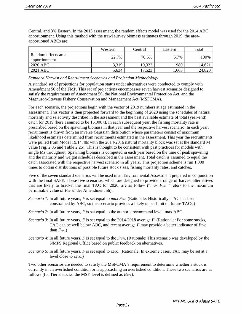
Central, and 3% Eastern. In the 2013 assessment, the random effects model was used for the 2014 ABC

apportionment. Using this method with the trawl survey biomass estimates through 2019, the area-

apportioned ABCs are:

Western Central Eastern Total

Random effects area

apportionment 22.7% 70.6% 6.7% 100%

2020 ABC 3,319 10,322 980 14,621

2021 ABC 5,634 17,523 1,663 24,820

Standard Harvest and Recruitment Scenarios and Projection Methodology

A standard set of projections for population status under alternatives were conducted to comply with

Amendment 56 of the FMP. This set of projections encompasses seven harvest scenarios designed to

satisfy the requirements of Amendment 56, the National Environmental Protection Act, and the

Magnuson-Stevens Fishery Conservation and Management Act (MSFCMA).

For each scenario, the projections begin with the vector of 2019 numbers at age estimated in the

assessment. This vector is then projected forward to the beginning of 2020 using the schedules of natural

mortality and selectivity described in the assessment and the best available estimate of total (year-end)

catch for 2019 (here assumed to be 15,000 t). In each subsequent year, the fishing mortality rate is

prescribed based on the spawning biomass in that year and the respective harvest scenario. In each year,

recruitment is drawn from an inverse Gaussian distribution whose parameters consist of maximum

likelihood estimates determined from recruitments estimated in the assessment. This year the recruitments

were pulled from Model 19.14.48c with the 2014-2016 natural mortality block was set at the standard M

value (Fig. 2.85 and Table 2.25). This is thought to be consistent with past practices for models with

single Ms throughout. Spawning biomass is computed in each year based on the time of peak spawning

and the maturity and weight schedules described in the assessment. Total catch is assumed to equal the

catch associated with the respective harvest scenario in all years. This projection scheme is run 1,000

times to obtain distributions of possible future stock sizes, fishing mortality rates, and catches.

Five of the seven standard scenarios will be used in an Environmental Assessment prepared in conjunction

with the final SAFE. These five scenarios, which are designed to provide a range of harvest alternatives

that are likely to bracket the final TAC for 2020, are as follow (“max FABC ” refers to the maximum

permissible value of FABC under Amendment 56):

Scenario 1: In all future years, F is set equal to max FABC. (Rationale: Historically, TAC has been

constrained by ABC, so this scenario provides a likely upper limit on future TACs.)

Scenario 2: In all future years, F is set equal to the author’s recommend level, max ABC.

Scenario 3: In all future years, F is set equal to the 2014-2018 average F. (Rationale: For some stocks,

TAC can be well below ABC, and recent average F may provide a better indicator of FTAC

than FABC.)

Scenario 4: In all future years, F is set equal to the F75%. (Rationale: This scenario was developed by the

NMFS Regional Office based on public feedback on alternatives.

Scenario 5: In all future years, F is set equal to zero. (Rationale: In extreme cases, TAC may be set at a

level close to zero.)

Two other scenarios are needed to satisfy the MSFCMA’s requirement to determine whether a stock is

currently in an overfished condition or is approaching an overfished condition. These two scenarios are as

follows (for Tier 3 stocks, the MSY level is defined as B35%):

Scenario 6: In all future years, F is set equal to FOFL. (Rationale: This scenario determines whether a stock

is overfished. If the stock is expected to be above half of its BMSY level in 2019 and above its

BMSY level in 2029 under this scenario, then the stock is not overfished.)

Scenario 7: In 2020 and 2021, F is set equal to max FABC, and in all subsequent years, F is set equal to

FOFL. (Rationale: This scenario determines whether a stock is approaching an overfished

condition. If the stock is 1) above its MSY level in 2021 or 2) above 1/2 of its MSY level in

2021 and expected to be above its MSY level in 2031 under this scenario, then the stock is

not approaching an overfished condition.)

Scenarios 1 through 7 were projected 13 years from 2019 in Model 19.14.48c (Table 2.28). Scenarios 3

and 5 (no fishing) project the stock to be below B35% until 2023, scenarios 1 and 2 have the stock below

B35% until 2024, and scenarios 6 and 7 have the stock below B35% until 2025. Fishing at the maximum

permissible rate indicate that the spawning stock (Fig. 2.86) will be below B35% in 2020 through 2024 due

to poor recruitment and high natural mortality post-2008. Under an assumption of mean recruitment, the

stock recovers above B35% by 2025.

Our projection model run under these conditions indicates that for Scenario 6, the GOA Pacific cod stock

although below B35% in 2020 at 32,957 t will be above its MSY value in 2030 at 70,555 t and therefore is

not overfished.

Projections 7 with fishing at the OFL after 2021 results in an expected spawning biomass of 70,313 t by

2031. These projections illustrate the impact of the low recruitment in 2015 and 2016. For example, under

all scenarios, the spawning biomass is expected to continue to drop in 2020 due to the low recruitments

post-2008 and high mortality of the 2011-2013 recruitments and decreasing influence of the high 2005-

2008 year classes and then levels off as the projection relies on mean recruitment post-2018.

Under Scenarios 6 (Fig. 2.86) and 7 of the 2019 Model 19.14.48c the projected spawning biomass for

Gulf of Alaska Pacific cod is not currently overfished, nor is it approaching an overfished status. However

the stock is below B20% triggering a closure of the directed Pacific cod fisheries managed under the GOA

FMP for 2020.

Ecosystem Considerations

Ecosystem Effects on the Stock

Food-web dynamics in the Gulf of Alaska (GOA) are structured by climate-driven changes to circulation

and water temperature, which can impact the distribution of key predators in the system and mediate

trophic interactions. Recent evaluation finds evidence for strong food-web responses to perturbation in the

GOA and indicates a dominance of destabilizing forces in the system that suggest a “dynamic ecosystem

structure, perhaps more prone to dramatic reorganization than the [Bering Sea], and perhaps inherently

less predictable” (Gaichas et al. 2015).

Predation is a major structuring pressure in the GOA ecosystem. Prey and predators of Pacific cod have

been described or reviewed by Albers and Anderson (1985), Livingston (1989, 1991), Lang et al. (2003),

Westerheim (1996), Yang (2004), and Gaichas et al. 2015. The composition of Pacific cod prey varies

spatially and with changing environmental conditions. In terms of percent occurrence, some of the most

important items in the diet of Pacific cod in the BSAI and GOA have been polychaetes, amphipods, and

crangonid shrimp. In terms of numbers of individual organisms consumed, some of the most important

dietary items have been euphausiids, miscellaneous fishes, and amphipods. In terms of weight of

organisms consumed, some of the most important dietary items have been walleye pollock, fishery offal,

yellowfin sole, and crustaceans (including Pandalidae and Chionoecetes bairdi). Predators of Pacific cod

include Pacific cod, halibut, salmon shark, northern fur seals, Steller sea lions, harbor porpoises, various

whale species, and tufted puffin. Major trends in the most important prey or predator species can be

expected to affect the dynamics of Pacific cod (Gaichas et al. 2015).

The marine heat wave of 2014-2016 in the Northeast Pacific was unprecedented in intensity, duration

(especially persistence of warm water through the winter months), and extent spatially and at depth (Bond

et al 2015). Metabolic demand for ectothermic fish like Pacific cod is largely a function of thermal

experience and tends to increase exponentially with increasing temperatures. Fish can minimize metabolic

costs through behaviors such as movement to thermally optimal temperatures (behavioral

thermoregulation), or can increase consumption of food energy to meet increasing metabolic demands.

The former requires sensory and swimming capability to move to favorable habitats (eggs and larvae

generally cannot), whereas the latter requires sufficient access to abundant or high energy prey resources.

The latter requires sufficient access to abundant or high energy prey resources. The former also requires

access to thermally optimal temperatures, which may not be available due to the recent marine heat wave.

Thus, metabolic costs due to warming may lead to decreased growth and survival when there is limited

access and availability to alternate food and thermal habitats.

When prey is readily available, Pacific cod consumption rates exhibit a non-linear relationship with

temperature, this non-linear response can limit foraging potential at very low and high temperatures. A

cumulative (over months) index based on this relationship indicates high potential foraging needs in the

GOA during the anomalously warm years of 2016-2019 (Fig. 2.87). Based on water temperatures at

preferred depth, foraging demand is greatest for smallest fish (Fig. 2.88), consistent with bioenergetic

estimates of metabolic demand from groundfish trawl surveys (diets, fish length, and bottom-temperature)

suggest higher metabolic demand for smaller fish (Fig 2.89).

Recent declines in Pacific cod biomass are most consistent with poor conditions for growth for 20-40 cm

fish (as well as 0-20cm fish). For this size range, bioenergetic model estimates of Pacific cod growth and

respiration suggest poor conditions for growth in 1998 (following the record El Niño of 1997/98), 2015,

and 2017 (middle panel Fig. 2.90) that were driven by high metabolic demand during those years (middle

panel, Fig. 2.89) and lower mean stomach fullness in recent years (height of columns in Fig. 2.91). Prey

energetic demand based on mean energy densities and annual shifts in diet composition show moderate

changes in diet energy density over time, with a general decline observed for 20-40 cm fish while recent

peaks in 2015 and 2017 are observed for 0-20 cm fish (Fig. 2.92). These could represent switching to

more energetic valuable prey and or increased rations (e.g., 2019). Stomach fullness (rations) in 2019 for

0-20 cm fish are the some of the highest observed (and follow one of the lowest levels observed in 2017);

for 20-40 cm fish 2019 rations continue to increase over 2015 and 2017 levels; there is no appreciable

trend in rations for 40-60 cm fish.

There are a few lines of evidence to support poor energetic conditions as a potential mechanism for

declines in Pacific cod abundance. First, poor fish condition was observed in 2015 (i.e., fish that were

lighter than average for a given length; Zador et al. 2017), potential growth in 2015 and 2016 is the lowest

in the time series, metabolic demands for 20-40 cm fish in 2015-2019 are the highest estimated (Fig.

2.89), and for 20-40 cm fish 2015-2019 diet energy density are below average (Fig. 2.92). Additionally

reports there have been numerous multi-trophic reports from 2015 to present day of mortality events from

starvation for avian and marine mammal predators that share prey resources with Pacific cod in the GOA.

Considered collectively, these lines of evidence suggest that persistent anomalously warm conditions that

extended from surface waters to depth, may have contributed to high mortality rates and overall

population decline for juvenile and adult Pacific cod from the years 2014-2019. Additional analysis of

these patterns is needed to further evaluate spatial differences in energetic demand and potential factors

influencing Pacific cod survival across the region.

From 9 September 2018 through 10 October 2019, the Gulf of Alaska again experienced heatwave

conditions above a 90th percentile threshold defined by Hobday et al. (2016). It’s reasonable to assume

that Pacific cod and other groundfish experienced similar metabolic pressures as during the beginning of

the 2014-2016 heatwave. The temperature profiles from the Gulf of Alaska bottom trawl survey suggest

that water temperatures in 2019 may have been as warm or warmer than those observed in 2015 and

2017, particularly near the surface in the western Gulf of Alaska (as reported by N. Laman in the 2019

GOA ESR). The 2019 anomaly profiles were most similar to 2015 profiles with warmer anomalies

(≥7.0oC) consistently observed across the entire survey area and penetrating to 200 m depths.

Fishery Effects on the Ecosystem

Potentially, fisheries for Pacific cod can have effects on other species in the ecosystem through a variety of

mechanisms, for example by relieving predation pressure on shared prey species (i.e., species which serve

as prey for both Pacific cod and other species), by reducing prey availability for predators of Pacific cod,

by altering habitat, by imposing bycatch mortality, or by “ghost fishing” caused by lost fishing gear.

Incidental Catch of Nontarget Species

Incidental catches of nontarget species in each year 2015-2019 are shown Table 2.7. In terms of average

catch over the time series, only sea stars account for more than 170 t per year.

Steller Sea Lions

Sinclair and Zeppelin (2002) showed that Pacific cod was one of the four most important prey items of

Steller sea lions in terms of frequency of occurrence averaged over years, seasons, and sites, and was

especially important in winter. Pitcher (1981) and Calkins (1998) also showed Pacific cod to be an

important winter prey item in the GOA and BSAI, respectively. Furthermore, the size ranges of Pacific cod

harvested by the fisheries and consumed by Steller sea lions overlap, and the fishery operates to some extent

in the same geographic areas used by Steller sea lion as foraging grounds (Livingston (ed.), 2002).

The Fisheries Interaction Team of the Alaska Fisheries Science Center was engaged in research to

determine the effectiveness of recent management measures designed to mitigate the impacts of the

Pacific cod fisheries (among others) on Steller sea lions. Results from studies conducted in 2002-2003

were summarized by Conners and Munro (2008). These studies included a tagging feasibility study,

which may evolve into an ongoing research effort capable of providing information on the extent and rate

to which Pacific cod move in and out of various portions of Steller sea lion critical habitat. Nearly 6,000

cod with spaghetti tags were released, of which approximately 1,000 had been returned as of September

2003.

Seabirds

The following is a summary of information provided by Livingston (ed., 2002): In both the BSAI and

GOA, the northern fulmar (Fulmarus glacialis) comprises the majority of seabird bycatch, which occurs

primarily in the longline fisheries, including the hook and line fishery for Pacific cod Shearwater

(Puffinus spp.) distribution overlaps with the Pacific cod longline fishery in the Bering Sea, and with

trawl fisheries in general in both the Bering Sea and GOA. Black-footed albatross (Phoebastria nigripes)

is taken in much greater numbers in the GOA longline fisheries than the Bering Sea longline fisheries, but

is not taken in the trawl fisheries. The distribution of Laysan albatross (Phoebastria immutabilis) appears

to overlap with the longline fisheries in the central and western Aleutians. The distribution of short-tailed

albatross (Phoebastria albatrus) also overlaps with the Pacific cod longline fishery along the Aleutian

chain, although the majority of the bycatch has taken place along the northern portion of the Bering Sea

shelf edge (in contrast, only two takes have been recorded in the GOA). Some success has been obtained

in devising measures to mitigate fishery-seabird interactions. For example, on vessels larger than 60 ft.

LOA, paired streamer lines of specified performance and material standards have been found to reduce

seabird incidental take significantly.

Fishery Usage of Habitat

The following is a summary of information provided by Livingston (ed., 2002): The longline and trawl

fisheries for Pacific cod each comprise an important component of the combined fisheries associated with

the respective gear type in each of the three major management regions (BS, AI, and GOA). Looking at

each gear type in each region as a whole (i.e., aggregating across all target species) during the period

1998-2001, the total number of observed sets was as follows:

Gear BS AI GOA

Trawl 240,347 43,585 68,436

Longline 65,286 13,462 7,139

In the BS, both longline and trawl effort was concentrated north of False Pass (Unimak Island) and along

the shelf edge represented by the boundary of areas 513, 517 (in addition, longline effort was concentrated

along the shelf edge represented by the boundary of areas 521-533). In the AI, both longline and trawl effort

were dispersed over a wide area along the shelf edge. The catcher vessel longline fishery in the AI occurred

primarily over mud bottoms. Longline catcher-processors in the AI tended to fish more over rocky bottoms.

In the GOA, fishing effort was also dispersed over a wide area along the shelf, though pockets of trawl

effort were located near Chirikof, Cape Barnabus, Cape Chiniak and Marmot Flats. The GOA longline

fishery for Pacific cod generally took place over gravel, cobble, mud, sand, and rocky bottoms, in depths

of 25 fathoms to 140 fathoms.

Impacts of the Pacific cod fisheries on essential fish habitat were further analyzed in an environmental

impact statement by NMFS (2005).

Gulf of Alaska Pacific cod Economic Performance Report for 2017

Pacific cod has been a critical species in the catch portfolio of the Gulf of Alaska (GOA) fisheries.

Starting in 2017, conservation reductions in the TAC have resulted in substantially reduced catch levels.

Between 2009-2016, Pacific cod typically accounted for just under 30% of the GOA’s FMP groundfish

harvest and over 20% of the total Pacific cod catch in Alaska. By 2018 these shares fell to approximately

6%. Catch of Pacific cod in the GOA was down 70% from 2017 with a total catch of 15.2 thousand t and

retained catch 14.4 thousand t (Table 2.27). Catches in 2019 are expected to be similarly constrained. Ex-

vessel revenues in 2018 were down 59% to $14.5 million with the reduction in catch (Table 2.27). The

products made from GOA Pacific cod had a first-wholesale value was $32 million in 2018, which was

down 58% from 2017 and below the 2009-2013 average of $102 million (Table 2.28).

The fishery for cod is an iconic fishery with a long history, particularly in the North Atlantic. Global catch

was consistently over 2 million t through the 1980s, but began to taper off in the 1990s as cod stocks

began to collapse in the northwest Atlantic Ocean. Over roughly the same period, the U.S. catch of

Pacific cod (caught in Alaska) grew to approximately 250 thousand tons where it remained throughout the

early to mid-2000s. European catch of Atlantic cod in the Barents Sea (conducted mostly by Russia,

Norway, and Iceland) slowed and global catch hit a low in 2007 at 1.13 million t. U.S. Pacific cod’s share

of global catch was at a high at just over 20% in the early 2000s. Since 2007 global catch has grown to

roughly 1.8 million t in recent years as catch in the Barents Sea has rebounded and U.S. catch has

remained strong at over 300 thousand t since 2011 (Table 2.29). European Atlantic cod and U.S. Pacific

cod remain the two major sources supplying the cod market over the past decade accounting for roughly

75% and 20%, respectively. Atlantic cod and Pacific cod are substitutes in the global market. Because of

cod’s long history, global demand is present in a number of geographical regions, but Europe and the U.S.

are the primary consumer markets for many of the Pacific cod products. The market for cod is also

indirectly affected by activity in the pollock fisheries which experienced a similar period of decline in

2008-2010 before rebounding. Cod and pollock are commonly used to produce breaded fish portions.

Alaska caught Pacific cod in the GOA became certified by the Marine Stewardship Council (MSC) in

2010, a NGO based third-party sustainability certification, which some buyers seek. Changes in global

catch and production account for much of the broader time trends in the cod markets. In particular, the

average first-wholesale prices peak approximately $1.90 per pound in 2008 and subsequently declined

precipitously to approximately $1.50 per pound in 2009-2010 as markets priced in consecutive years of

approximately 100 thousand t increases in the Barents Sea cod catch in 2009-2011; coupled with reduced

demand from the recession.

The Pacific cod total allowable catch (TAC) is allocated to multiple sectors. In the GOA, sectors are

defined by gear type (hook and line, pot, trawl and jig) and processing capacity (catcher vessel (CV) and

catcher processor (CP)). Within the sectoral allocations the fisheries effectively operate as open access

with limited entry. The majority of GOA Pacific cod is caught by CVs which make deliveries to shore-

based processors and accounts for 90% of the total GOA Pacific cod catch (Table 1). Approximately 25%

is caught by the trawl, 55% is caught by pot gear, and 20% caught by hook and line, though the number

of hook and line vessels is far greater. Poor fishing conditions in 2017 may have contributed to the

significant reduction in jig fleet participation in 2017. Prior to 2016, approximately 60% of the retained

catch volume and value is in the Central Gulf fisheries, 40% in the Western Gulf, and 1-2% occurring in

other region of the GOA. Since 2016 the distribution has shifted to about 50% with proportionally more

cod is being caught in the Western Gulf. Harvests from catcher vessels that deliver to shoreside

processors account for approximately 90% of the retained catch. The 2018 retained catch in the GOA

decreased 70% to 14.4 thousand t. The ex-vessel value totaled $14.5 million in 2018, which was down

from $35 million in 2017 (Table 2.27). Ex-vessel prices increased 35% to $0.45 per pound in 2018. Catch

from the fixed gear vessels (which includes hook-and-line and pot gear) typically receive a slightly higher

price from processors because they incur less damage when caught. This price differential was $0.05 per

pound in 2018.

The first-wholesale value of Pacific cod products was down 58% to $32 million in 2018 (Table 2.28).

Despite lower prices through 2014 and 2015 revenues were strong as result of increased catch levels. In

contrast, in 2016-2018 prices were up and there was a decrease in revenues as a result of reduced

production volumes. The two primary product forms produced from cod in the GOA are fillets and H&G,

which comprised approximately 60% and 30% of the value in 2018, though the relative share can

fluctuate year over year depending on relative prices and processing decisions. The average price of GOA

Pacific cod products in 2018 increased 32% to $2.60 per pound as fillet prices increase 38% to $4.35 per

pound and H&G prices increased 36% to $2.05 per pound (Table 2.28). Since 2016 reductions in global

supply have put upward pressure on prices resulting in significant year over year price increases in 2017

and 2018. Available information on 2019 prices indicate that prices may be leveling off as reflected in the

highly exported H&G product type where the price through June of 2019 fell 2%.

U.S. exports of cod are roughly proportional to U.S. cod production. More than 90% of the exports are

H&G, much of which goes to China for secondary processing and re-export (Table 2.29). China’s rise as

re-processor is fairly recent. Between 2001 and 2011 exports to China have increased nearly 10 fold and

continued to increase up to 2016. Since 2017 China’s share of exports has declined slightly going from

55% in 2016 to 47% in 2018. The cod industry has largely avoided U.S. tariffs that would have a

significant negative impact on them in the U.S.-China trade war. However, Chinese tariffs on U.S.

products could inhibit growth in that market. Japan and Europe (mostly Germany and the Netherlands)

are also important export destinations. Japan and Europe accounted for 15% and 16% of the export

volume respectively. Approximately 30% of Alaska’s cod production is estimated to remain in the U.S..

Because U.S. cod production is approximately 20% of global production and the GOA is approximately

6% of U.S. production, the GOA Pacific cod is a relatively small component of the broader cod market.

Strong demand and tight supply in 2017-2018 from the U.S. and globally have contributed to increasing

prices. The Barents Sea quota was reduced by 13% 2018 and the global cod supply will remain

constrained. Groundfish forum estimates for 2019 indicate global catches of Atlantic and Pacific cod will

be reduced by approximately 100 thousand t. Markets may have incorporated these supply adjustments as

export prices in 2019 have leveled off, decreasing slightly by 2% (Table 2.29). A portion of the Russian

catch of Pacific cod became MSC certified in Oct. 2019 which could put further downward pressure on

prices going forward.

Data Gaps and Research Priorities

Understanding of the above ecosystem considerations would be improved if future research were directed

toward closing certain data gaps. Such research would have several foci, including the following: 1)

ecology of the Pacific cod stock, including spatial dynamics, trophic and other interspecific relationships,

and the relationship between climate and recruitment; 2) behavior of the Pacific cod fishery, including

spatial dynamics; 3) determinants of trawl survey catchability and selectivity and relationship with

environmental covariates; 4) age determination and effects of aging error and bias on model parameters

including natural mortality; 5) ecology of species taken as bycatch in the Pacific cod fisheries, including

estimation of biomass, carrying capacity, and resilience; and 6) ecology of species that interact with

Pacific cod, including estimation of biomass, carrying capacity, and resilience.

Literature Cited

Abookire, A. A., J. T. Duffy-Anderson, and C. M. Jump. 2007. Habitat associations and diet of young-of-

the-year Pacific cod (Gadus macrocephalus) near Kodiak, Alaska. Marine Biology 150:713-726.

Albers, W. D., and P. J. Anderson. 1985. Diet of Pacific cod, Gadus macrocephalus, and predation on the

northern pink shrimp, Pandalus borealis, in Pavlof Bay, Alaska. Fish. Bull., U.S. 83:601-610.

Alderdice, D.F. and C. R. Forrester, 1971. Effects of salinity, temperature, and dissolved oxygen on early

development of the Pacific cod (Gadus macrocephalus). Journal of the Fisheries Board of

Canada, 28(6), pp.883-902.

A’mar, T. and W. Pallson 2015. Assessment of the Pacific cod stock in the Gulf of Alaska. In Plan Team

for Groundfish Fisheries of the Gulf of Alaska (compiler), Stock assessment and fishery

evaluation report for the groundfish resources of the Gulf of Alaska, p. 173-296. North Pacific

Fishery Management Council, 605 W. 4th Avenue Suite 306, Anchorage, AK 99501

Bakkala, R. G., and V. G. Wespestad. 1985. Pacific cod. In R. G. Bakkala and L. L. Low (editors),

Condition of groundfish resources of the eastern Bering Sea and Aleutian Islands region in 1984,

p. 37-49. U.S. Dep. Commer., NOAA Tech. Memo. NMFS F/NWC-83.

Barbeaux. S. J., K. Aydin, B. Fissel, K. Holsman, W. Palsson, K. Shotwell, Q. Yang, and S. Zador. 2018.

Assessment of the Pacific cod stock in the Gulf of Alaska. In Plan Team for Groundfish Fisheries

of the Gulf of Alaska (compiler), Stock assessment and fishery evaluation report for the

groundfish resources of the Gulf of Alaska. North Pacific Fishery Management Council, 605 W.

4th Avenue Suite 306, Anchorage, AK 99501

Barbeaux. S. J., A’mar, T., and Palsson, W. 2016. Assessment of the Pacific cod stock in the Gulf of Alaska. In Plan Team for Groundfish Fisheries of the Gulf of Alaska (compiler), Stock

assessment and fishery evaluation report for the groundfish resources of the Gulf of Alaska, p.

175-324. North Pacific Fishery Management Council, 605 W. 4th Avenue Suite 306, Anchorage,

AK 99501

Baty, F., Ritz, C. Charles, S., Brutsche, M., Flandrois, J., Delignette-Muller, M. 2015. A Toolbox for

Nonlinear Regression in R: The Package nlstools. Journal of Statistical Software, 66(5), 1-21.

URL http://www.jstatsoft.org/v66/i05/

Betts, M., H. D. G. Maschner, and D. S. Clark 2011. Zooarchaeology of the ‘Fish That Stops’, in

Madonna L. Moss and Aubrey Cannon, eds., The Archaeology of North Pacific Fisheries,

University of Alaska Press, Fairbanks, Alaska, 188.

Bond, N. A., M. F. Cronin, H. Freeland, and N. Mantua. 2015. Causes and impacts of the 2014 warm

anomaly in the NE Pacific. Geophys. Res. Lett., 42, 3414–3420

Cahalan, J., J. Gasper, and J. Mondragon. 2014. Catch sampling and estimation in the federal groundfish

fisheries off Alaska, 2015 edition. U.S. Dep. Commer., NOAA Tech. Memo. NMFS-AFSC-286,

46 p.

Calkins, D. G. 1998. Prey of Steller sea lions in the Bering Sea. Biosphere Conservation 1:33-44.

Conners, M.E. and Munro, P., 2008. Effects of commercial fishing on local abundance of Pacific cod

(Gadus macrocephalus) in the Bering Sea. Fishery Bulletin, 106(3), pp.281-292.

Copeman, L. A., and B. J. Laurel. 2010. Experimental evidence of fatty acid limited growth and survival

in Pacific cod larvae. Marine Ecology Progress Series 412:259-272.

Copeman, L. A., B. J. Laurel, M. Spencer, and A. Sremba. 2017. Temperature impacts on lipid allocation

among juvenile gadid species at the Pacific Arctic-Boreal interface: an experimental laboratory

approach. Marine Ecology Progress Series 566:183-198.

Doyle, M. J., and K. L. Mier. 2016. Early life history pelagic exposure profiles of selected commercially

important fish species in the Gulf of Alaska. Deep-Sea Research Part Ii-Topical Studies in

Oceanography 132:162-193.

Doyle, M. J., S. J. Picquelle, K. L. Mier, M. C. Spillane, and N. A. Bond. 2009. Larval fish abundance

and physical forcing in the Gulf of Alaska, 1981-2003. Progress in Oceanography 80:163-187.

Drinan, D.P., Gruenthal, K.M., Canino, M.F., Lowry, D., Fisher, M.C. and Hauser, L., 2018.

Population assignment and local adaptation along an isolation‐by‐distance gradient in

Pacific cod (Gadus macrocephalus). Evolutionary applications, 11(8), pp.1448-1464.

Echave KB, Hanselman DH, Adkison MD, Sigler MF. 2012. Inter-decadal changes in sablefish,

Anoplopoma fimbria, growth in the northeast Pacific Ocean. Fish. Bull. 210: 361-374

Faunce, C., J. Sullivan, S. Barbeaux, J. Cahalan, J. Gasper, S. Lowe, and R. Webster. 2017. Deployment

performance review of the 2016 North Pacific Groundfish and Halibut Observer Program. U.S.

Dep. Commer., NOAA Tech. Memo. NMFS-AFSC-358, 75 p.

Fournier, D. 1983. An analysis of the Hecate Strait Pacific cod fishery using an age-structured model

incorporating density-dependent effects. Can. J. Fish. Aquat. Sci. 40:1233-1243.

Fournier, D., and C. P. Archibald. 1982. A general theory for analyzing catch at age data. Can. J. Fish.

Aquat. Sci. 38:1195-1207.

Fournier, D.A., H. J. Skaug, J. Ancheta, J. Ianelli, A. Magnusson, M. N. Maunder, A. Nielsen, and J.

Sibert. 2012. AD Model Builder: using automatic differentiation for statistical inference of highly

parameterized complex nonlinear models. Optim. Methods Softw. 27:233-249.

Gaichas, S., Aydin, K.Y. & Francis, R.C. 2015. Wasp waist or beer belly? Modeling food web structure

and energetic control in Alaskan marine ecosystems, with implications for fishing and

environmental forcing. Progress in Oceanography, 138: 1–17.

https://doi.org/10.1016/j.pocean.2015.09.010

Geweke, J. 1992. Evaluating the accuracy of sampling-based approaches to calculating posterior

moments. In Bayesian Statistics 4 (ed JM Bernado, JO Berger, AP Dawid and AFM Smith).

Clarendon Press, Oxford, UK.

Hanselman, D.H., C.R. Lunsford, C.J. Rodgveller, and M.J. Peterson. 2016. Assessment of the sablefish

stock in Alaska. In Stock assessment and fishery evaluation report for the groundfish resources of

the GOA and BS/AI. North Pacific Fishery Management Council, 605 W 4th Ave, Suite 306

Anchorage, AK 99501. pp. 325-488.

Heidelberger P and Welch PD. Simulation run length control in the presence of an initial transient. Opns

Res., 31, 1109-44 (1983)

Hobday, A.J., Alexander, L.V., Perkins, S.E., Smale, D.A., Straub, S.C., Oliver, E.C., Benthuysen, J.A.,

Burrows, M.T., Donat, M.G., Feng, M. and Holbrook, N.J., 2016. A hierarchical approach to

defining marine heatwaves. Progress in Oceanography, 141, pp.227-238.Holsman, KK and K

Aydin. 2015. Comparative methods for evaluating climate change impacts on the foraging

ecology of Alaskan groundfish. Mar Ecol Prog Ser doi: 521:217-23510.3354/ meps11102

Hobday, A.J., Oliver, E.C., Gupta, A.S., Benthuysen, J.A., Burrows, M.T., Donat, M.G., Holbrook, N.J.,

Moore, P.J., Thomsen, M.S., Wernberg, T. and Smale, D.A., 2018. Categorizing and naming

marine heatwaves. Oceanography, 31(2), pp.162-173.

Hurst, T. P., D. W. Cooper, J. S. Scheingross, E. M. Seale, B. J. Laurel, and M. L. Spencer. 2009. Effects

of ontogeny, temperature, and light on vertical movements of larval Pacific cod (Gadus

macrocephalus). Fisheries Oceanography 18:301-311.

Hurst, T. P., B. J. Laurel, and L. Ciannelli. 2010. Ontogenetic patterns and temperature-dependent growth

rates in early life stages of Pacific cod (Gadus macrocephalus). Fishery Bulletin 108:382-392.

Jensen, A.L., 1996. Beverton and Holt life history invariants result from optimal trade-off of reproduction

and survival. Canadian Journal of Fisheries and Aquatic Sciences, 53(4), pp.820-822.

Kastelle, C.R., Helser, T.E., McKay, J.L., Johnston, C.G., Anderl, D.M., Matta, M.E. and Nichol, D.G.,

2017. Age validation of Pacific cod (Gadus macrocephalus) using high-resolution stable oxygen

isotope (δ 18O) chronologies in otoliths. Fisheries research, 185, pp.43-53.

Ketchen, K.S. 1964. Preliminary results of studies on a growth and mortality of Pacific cod (Gadus

macrocephalus) in Hecate Strait, British Columbia. J. Fish. Res. Bd. Canada 21:1051-1067.

Kimura, D.K., Balsiger, J.W. and Ito, D.H., 1984. Generalized stock reduction analysis. Canadian Journal

of Fisheries and Aquatic Sciences, 41(9), pp.1325-1333.

Lang, G. M., C. W. Derrah, and P. A. Livingston. 2003. Groundfish food habits and predation on

commercially important prey species in the Eastern Bering Sea from 1993 through 1996. Alaska

Fisheries Science Center Processed Report 2003-04. Alaska Fisheries Science Center, 7600 Sand

Point Way NE., Seattle, WA 98115-6349. 351 p.

Laurel, B., M. Spencer, P. Iseri, and L. Copeman. 2016a. Temperature-dependent growth and behavior of

juvenile Arctic cod (Boreogadus saida) and co-occurring North Pacific gadids. Polar Biology

39:1127-1135.

Laurel, B. J., D. Cote, R. S. Gregory, L. Rogers, H. Knutsen, and E. M. Olsen. 2017. Recruitment signals

in juvenile cod surveys depend on thermal growth conditions. Canadian Journal of Fisheries and

Aquatic Sciences 74:511-523.

Laurel, B. J., T. P. Hurst, and L. Ciannelli. 2011. An experimental examination of temperature

interactions in the match-mismatch hypothesis for Pacific cod larvae. Canadian Journal of

Fisheries and Aquatic Sciences 68:51-61.

Laurel, B. J., T. P. Hurst, L. A. Copeman, and M. W. Davis. 2008. The role of temperature on the growth

and survival of early and late hatching Pacific cod larvae (Gadus macrocephalus). Journal of

Plankton Research 30:1051-1060.

Laurel, B. J., B. A. Knoth, and C. H. Ryer. 2016b. Growth, mortality, and recruitment signals in age-0

gadids settling in coastal Gulf of Alaska. ICES Journal of Marine Science 73:2227-2237.

Laurel and Rogers (in revision) Loss of spawning habitat and pre-recruits of Pacific cod during a Gulf of

Alaska heatwave. Can J Fish Aquat.

Laurel, B. J., C. H. Ryer, B. Knoth, and A. W. Stoner. 2009. Temporal and ontogenetic shifts in habitat

use of juvenile Pacific cod (Gadus macrocephalus). Journal of Experimental Marine Biology and

Ecology 377:28-35.

Laurel, J., A. W. Stoner, C. H. Ryer, T. P. Hurst, and A. A. Abookire. 2007. Comparative habitat

associations in juvenile Pacific cod and other gadids using seines, baited cameras and laboratory

techniques. Journal of Experimental Marine Biology and Ecology 351:42-55.Livingston, P. A.

1989. Interannual trends in Pacific cod, Gadus macrocephalus, predation on three commercially

important crab species in the eastern Bering Sea. Fish. Bull., U.S. 87:807-827.

Li, L., Hollowed, A.B., Cokelet, E.D., Barbeaux, S.J., Bond, N.A., Keller, A.A., King, J.R., McClure,

M.M., Palsson, W.A., Stabeno, P.J. and Yang, Q., 2019. Subregional differences in groundfish

distributional responses to anomalous ocean bottom temperatures in the northeast Pacific. Global

change biology.

Litzow M, Abookire A. 2018. Kodiak and Alaska Peninsula Cruise Report, College of Fisheries and

Ocean Sciences, University of Alaska Fairbanks pgs 1-3

Livingston, P.A., 1989. Interannual trends in Pacific cod, Gadus macrocephalus, predation on three

commercially important crab species in the eastern Bering Sea. Fishery Bulletin, 87(4), pp.807-

827.

Livingston, P. A. 1991. Pacific cod. In P. A. Livingston (editor), Groundfish food habits and predation on

commercially important prey species in the eastern Bering Sea from 1984 to 1986, p. 31-88. U.S.

Dept. Commer, NOAA Tech. Memo. NMFS F/NWC-207.

Livingston, P. A. (editor). 2003. Ecosystem Considerations for 2003. North Pacific Fishery Management

Council, 605 West 4th Ave., Suite 306, Anchorage, AK 99501.

Livingston, P.A., Aydin, K., Buckley, T.W., Lang, G.M., Yang, M-S., Miller, B.S. (2017) Quantifying

food web interactions in the North Pacific - a data-based approach. Environmental Biology of

Fishes 100:443-470. doi: 10.1007/s10641-017-0587-0

Low, L. L. 1974. A study of four major groundfish fisheries of the Bering Sea. Ph.D. Thesis, Univ.

Washington, Seattle, WA. 240 p.

Matarese, A. C., D. M. Blood, S. J. Picquelle, and J. L. Benson. 2003. Atlas of abundance and distribution

patterns of ichthyoplankton from the Northeast Pacific Ocean and Bering Sea ecosystems: based

on research conducted by the Alaska Fisheries Science Center (1972–1996).

Methot, R. D. 1986. Synthetic estimates of historical abundance and mortality for northern anchovy,

Engraulis mordax. NMFS, Southwest Fish. Cent., Admin. Rep. LJ 86-29, La Jolla, CA.

Methot, R. D. 1990. Synthesis model: An adaptable framework for analysis of diverse stock assessment

data. Int. N. Pac. Fish. Comm. Bull. 50:259-277.

Methot, R. D. 2005. User manual for the assessment program Strock Synthesis 2 (SS2), Model Version

1.19. National Marine Fisheries Service, Northwest Fisheries Science Center, 2725 Montlake

Blvd. East, Seattle, WA 98112-2097. 47 p.

Methot, R. D. 2007. User manual for the integrated analysis program Stock Synthesis 2 (SS2), Model

Version 2.00c. National Marine Fisheries Service, Northwest Fisheries Science Center, 2725

Montlake Blvd. East, Seattle, WA 98112-2097. 47 p.

Methot, R. D., and Wetzell, C. R. 2013. Stock synthesis: A biological and statistical framework for fish

stock assessment and fishery management. Fish. Rsch. 142:86-99.

Moss, J. H., M. F. Zaleski, and R. A. Heintz. 2016. Distribution, diet, and energetic condition of age-0

walleye pollock (Gadus chalcogrammus) and pacific cod (Gadus macrocephalus) inhabiting the

Gulf of Alaska. Deep-Sea Research Part Ii-Topical Studies in Oceanography 132:146-153.

Mukhina, N.V., Marshall, C.T. and Yaragina, N.A., 2003. Tracking the signal in year-class strength of

Northeast Arctic cod through multiple survey estimates of egg, larval and juvenile abundance.

Journal of Sea Research, 50(1), pp.57-75.

Nash, R.D., Valencia, A.H. and Geffen, A.J., 2006. The origin of Fulton’s condition factor—setting the

record straight. Fisheries, 31(5), pp.236-238.

National Marine Fisheries Service (NMFS). 2005. Final environmental impact statement for essential fish

habitat identification and conservation in Alaska. National Marine Fisheries Service, Alaska

Region. P.O. Box 21668, Juneau, AK 99802-1668.

National Oceanographic and Atmospheric Administration (NOAA). 2017. NOAA OI SST V2 High

Resolution Dataset. Available:

https://www.esrl.noaa.gov/psd/data/gridded/data.noaa.oisst.v2.highres.html

Nichols, N. W., P. Converse, and K. Phillips. 2015. Annual management report for groundfish fisheries in

the Kodiak, Chignik, and South Alaska Peninsula Management Areas, 2014. Alaska Department

of Fish and Game, Fishery Management Report No. 15-41, Anchorage.

Pitcher, K. W. 1981. Prey of Steller sea lion, Eumetopias jubatus, in the Gulf of Alaska. Fishery Bulletin

79:467-472.

Plummer, M., Best, N., Cowles, K. and Vines K. 2006. CODA: Convergence Diagnosis and Output

Analysis for MCMC, R News, vol 6, 7-11

Raring, N. W., E. A. Laman, P. G. von Szalay, and M. H. Martin. 2016. Data report: 2011 Gulf of Alaska

bottom trawl survey. U.S. Dep. Commer., NOAA Tech. Memo. NMFS-AFSC-330, 231 p.

doi:10.7289/V5/TM-AFSC-330.

Rose, G.A. and Kulka, D.W., 1999. Hyperaggregation of fish and fisheries: how catch-per-unit-effort

increased as the northern cod (Gadus morhua) declined. Canadian Journal of Fisheries and

Aquatic Sciences, 56(S1), pp.118-127.

Rutecki, T. L., and Varosi, E. R. 1997. Distribution, age, and growth of juvenile sablefish, Anoplopoma fimbria, in southeast Alaska. U.S. Dep. Commer., NOAA Technical Report NMFS, vol. 130, pp.

45– 54.

Saha, S., and Coauthors, 2010: The NCEP climate forecast system reanalysis. Bull. Amer. Meteor. Soc.,

91, 1015-1057.

Sasaki, T., 1985. Studies on the sablefish resources in the North Pacific Ocean. Far Seas Fishery

Laboratory Bulletin, 22, pp. 1–108. Shimizu, 424, Japan.

Schlegel, R.W. and Smit, A.J., 2018. heatwaveR: A central algorithm for the detection of heatwaves and

cold-spells. J. Open Source Software, 3(27), p.821.

Shimada, A. M., and D. K. Kimura. 1994. Seasonal movements of Pacific cod (Gadus macrocephalus) in

the eastern Bering Sea and adjacent waters based on tag-recapture data. U.S. Natl. Mar. Fish.

Serv., Fish. Bull. 92:800-816.

Sigler, M. F. and Fujioka, J. T., 1988. Evaluation of variability in sablefish, Anoplopoma fimbria,

abundance indices in the Gulf of Alaska using the boarstrap method. Fishery Bulletin, 86(3).

Sigler, M.F., and Zenger, H.H. 1989. Assessment of Gulf of Alaska sablefish and other groundfish based

on the domestic longline survey, 1987. NOAA Tech. Memo. NMFS F/NWC-169.

Sinclair, E.S. and T. K. Zeppelin. 2002. Seasonal and spatial differences in diet in the western stock of

Steller sea lions (Eumetopias jubatus). Journal of Mammalogy 83(4).

Soderlund, E., Dykstra, C., Geernaert, T., Anderson-Chao, E., Ranta, A. 2009. 2008 Standardized stock

assessment survey. Int. Pac. Halibut Comm. Report of Assessment and Research Activities 2008:

469-496

Smith, R.L., Paul, A.J. and Paul, J.M., 1990. Seasonal changes in energy and the energy cost of spawning

in Gulf of Alaska Pacific cod. Journal of Fish Biology, 36(3), pp.307-316.

Spalinger, K., 2006. Bottom trawl survey of crab and groundfish: Kodiak, Chignik, South Peninsula, and

eastern Aleutian management districts, 2005. Alaska Department of Fish and Game, Division of

Sport Fish, Research and Technical Services.

Spies I. 2012. Landscape genetics reveals population subdivision in Bering Sea and Aleutian Islands

Pacific cod. Transactions of the American Fisheries Society 141:1557-1573.

Spies, I., Gruenthal, K., Drinan, D., Hollowed, A., Stevenson, D., Tarpey, C., and Hauser, L. 2019.

Genetic evidence of a northward range expansion in the eastern Bering Sea stock of Pacific cod.

Evolutionary Applications. doi: 10.1111/EVA.12874.

Stark, J. W. 2007. Geographic and seasonal variations in maturation and growth of female Pacific cod

(Gadus macrocephalus) in the Gulf of Alaska and Bering Sea. Fish. Bull. 105:396–407.

Stauffer, G. 2004. NOAA protocols for groundfish bottom trawl surveys of the Nation’s fishery

resources. U.S. Dep. Commer., NOAA Tech. Memo. NMFS-F/SPO-65, 205 p.

Strasburger, W. W., N. Hillgruber, A. I. Pinchuk, and F. J. Mueter. 2014. Feeding ecology of age-0

walleye pollock (Gadus chalcogrammus) and Pacific cod (Gadus macrocephalus) in the

southeastern Bering Sea. Deep-Sea Research Part Ii-Topical Studies in Oceanography 109:172-

180.

Thompson, G.G. 2017. Assessment of the Pacific Cod Stock in the Eastern Bering Sea. In Stock

assessment and fishery evaluation report for the groundfish resources of the Gulf of Alaska

[online]. Compiled by The Plan Team for the Groundfish Fisheries of the Gulf of Alaska. North

Pacific Fishery Management Council, Anchorage, Alaska.

Thompson, G., T. A’mar, and W. Palsson. 2011. Assessment of the Pacific cod stock in the Gulf of

Alaska. In Plan Team for Groundfish Fisheries of the Gulf of Alaska (compiler), Stock

assessment and fishery evaluation report for the groundfish resources of the Gulf of Alaska, p.

161-306. North Pacific Fishery Management Council, 605 W. 4th Avenue Suite 306, Anchorage,

AK 99501

Thompson, G. G., and M. E. Conners. 2007. Report of the Pacific cod technical workshop held at the

Alaska Fisheries Science Center, April 24-25, 2007. Unpubl. manuscr., Alaska Fisheries Science

Center, Resource Ecology and Fisheries Management Division, 7600 Sand Point Way NE.,

Seattle, WA 98115-6349. 56 p.

Thompson, G. G., and M. W. Dorn. 2005. Assessment of the Pacific cod stock in the Gulf of Alaska. In

Plan Team for Groundfish Fisheries of the Gulf of Alaska (compiler), Stock assessment and

fishery evaluation report for the groundfish resources of the Gulf of Alaska, p. 155-244. North

Pacific Fishery Management Council, 605 W. 4th Avenue Suite 306, Anchorage, AK 99501.

Thompson, G. G., and R. D. Methot. 1993. Pacific cod. In Plan Team for Groundfish Fisheries of the

Bering Sea/Aleutian Islands (editor), Stock assessment and fishery evaluation report for the

groundfish resources of the Bering Sea/Aleutian Islands region as projected for 1994, chapter 2.

North Pacific Fishery Management Council, 605 W. 4th Avenue Suite 306, Anchorage, AK

99501.

Thompson, G. G., and A. M. Shimada. 1990. Pacific cod. In L. L. Low and R. E. Narita (editors),

Condition of groundfish resources of the eastern Bering Sea-Aleutian Islands region as assessed

in 1988, p. 44-66. U.S. Dep. Commer., NOAA Tech. Memo. NMFS F/NWC-178.

Thompson, G. G, and H. H. Zenger. 1993. Pacific cod. In Plan Team for Groundfish Fisheries of the Gulf

of Alaska (editor), Stock assessment and fishery evaluation report for the groundfish resources of the Gulf of Alaska as projected for 1994, chapter 2. North Pacific Fishery Management Council,

605 W. 4th Avenue Suite 306, Anchorage, AK 99501.Voesenek, C. J., F. T. Muijres, and J. L.

van Leeuwen. 2018. Biomechanics of swimming in developing larval fish. Journal of

Experimental Biology 221.

von Biela, V.R., Arimitsu, M.L., Piatt, J.F., Heflin, B., Schoen, S.K., Trowbridge, J.L. and Clawson,

C.M., 2019. Extreme reduction in nutritional value of a key forage fish during the Pacific marine

heatwave of 2014-2016. Marine Ecology Progress Series, 613, pp.171-182.

von Szalay, P.G., and N.W. Raring. 2018. Data report: 2017 Gulf of Alaska bottom trawl survey. NOAA

Tech. Mem NMFS-AFSC-374. 260 p.

Walters, C., 2003. Folly and fantasy in the analysis of spatial catch rate data. Canadian Journal of

Fisheries and Aquatic Sciences, 60(12), pp.1433-1436.

Wespestad, V., R. Bakkala, and J. June. 1982. Current abundance of Pacific cod (Gadus macrocephalus)

in the eastern Bering Sea and expected abundance in 1982-1986. NOAA Tech. Memo. NMFS

F/NWC-25, 26 p.

Westrheim, S. J. 1996. On the Pacific cod (Gadus macrocephalus) in British Columbia waters, and a comparison with Pacific cod elsewhere, and Atlantic cod (G. morhua). Can. Tech. Rep. Fish.

Aquat. Sci. 2092. 390 p.

Yang, M-S. 2004. Diet changes of Pacific cod (Gadus macrocephalus) in Pavlof Bay associated with

climate changes in the Gulf of Alaska between 1980 and 1995. U.S. Natl. Mar. Fish. Serv., Fish.

Bull. 102:400-405.

Yang, Q., Cokelet, E.D., Stabeno, P.J., Li, L., Hollowed, A.B., Palsson, W.A., Bond, N.A. and Barbeaux,

S.J., 2019. How “The Blob” affected groundfish distributions in the Gulf of Alaska. Fisheries

Oceanography, 28(4), pp.434-453.

Zador et al. 2017. Ecosystem considerations for the Gulf of Alaska. 2017 SAFE report.

Tables

Table 2.1. Studies of Pacific cod natural mortality and statistics on the combined values. Use? Column indicates

whether the value was used in developing this year’s assessment model prior on natural mortality.

Area Author Year Value ln(value) Use? Statistics

EBS Low 1974 0.375 -0.981 Y mu: -0.815

EBS Wespestad et al. 1982 0.7 -0.357 Y sigma: 0.423

EBS Bakkala and Wespestad 1985 0.45 -0.799 Y Arithmetic: 0.484

EBS Thompson and Shimada 1990 0.29 -1.238 Y Geometric: 0.443

EBS Thompson and Methot 1993 0.37 -0.994 Y Harmonic: 0.405

EBS Shimada and Kimura 1994 0.96 -0.041 Y Mode: 0.370

EBS Shi et al. 2007 0.45 -0.799 Y L95%: 0.193

EBS Thompson et al. 2007 0.34 -1.079 Y U95%: 1.015

EBS Thompson 2016 0.36 -1.022 Y

GOA Thompson and Zenger 1993 0.27 -1.309 Y

GOA Thompson and Zenger 1995 0.5 -0.693 Y

GOA Thompson 2007 0.38 -0.968 Y

GOA Barbeaux et al. 2016 0.47 -0.755 N

BC Ketchen 1964 0.595 -0.519 Y

BC Fournier 1983 0.65 -0.431 Y

Table 2.2. Catch (t) for 1991 through 2019 by jurisdiction and gear type (as of 2019-10-02)

Federal State

Year Trawl

Long-

line Pot Other Subtotal

Long-

line Pot Other Subtotal Total 1991 58,093 7,656 10,464 115 76,328 0 0 0 0 76,328

1992 54,593 15,675 10,154 325 80,747 0 0 0 0 80,747

1993 37,806 8,963 9,708 11 56,488 0 0 0 0 56,488

1994 31,447 6,778 9,161 100 47,485 0 0 0 0 47,485

1995 41,875 10,978 16,055 77 68,985 0 0 0 0 68,985

1996 45,991 10,196 12,040 53 68,280 0 0 0 0 68,280

1997 48,406 10,978 9,065 26 68,476 0 7,224 1,319 8,542 77,018

1998 41,570 10,012 10,510 29 62,121 0 9,088 1,316 10,404 72,525

1999 37,167 12,363 19,015 70 68,614 0 12,075 1,096 13,171 81,785

2000 25,443 11,660 17,351 54 54,508 0 10,388 1,643 12,031 66,560

2001 24,383 9,910 7,171 155 41,619 0 7,836 2,084 9,920 51,542

2002 19,810 14,666 7,694 176 42,345 0 10,423 1,714 12,137 54,483

2003 18,884 9,525 12,765 161 41,335 62 7,943 3,242 11,247 52,582 2004 17,513 10,326 14,966 400 43,205 51 10,602 2,765 13,419 56,624 2005 14,549 5,732 14,749 203 35,233 26 9,653 2,673 12,351 47,584 2006 13,132 10,244 14,540 118 38,034 55 9,146 662 9,863 47,897 2007 14,775 11,539 13,573 44 39,932 270 11,378 682 12,329 52,261 2008 20,293 12,106 11,230 63 43,691 317 13,438 1,568 15,323 59,014 2009 13,976 13,968 11,951 206 40,101 676 9,919 2,500 13,096 53,196 2010 21,765 16,540 20,116 429 58,850 826 14,604 4,045 19,475 78,325, 2011 16,453 16,668 29,233 722 63,076 1,035 16,675 4,627 22,337 85,412 2012 20,072 14,467 21,238 722 56,499 866 15,940 4,613 21,419 77,918 2013 21,700 12,866 17,011 476 52,053 1,089 14,156 1,303 16,547 68,600 2014 26,798 14,749 19,957 1,046 62,550 1,007 18,445 2,838 22,290 84,841 2015 22,269 13,054 20,653 408 56,384 578 19,719 2,808 23,104 79,489 2016 15,217 8,153 19,248 346 42,964 806 18,609 1,708 21,123 64,087 2017 13,041 8,978 13,426 67 35,512 149 13,011 62 13,222 48,734 2018 3,819 3,130 4,014 120 11,084 309 3,660 195 4,163 15,247

2019* 3,826 2,602 2,604 175 9,207 285 3,551 329 4,166 13,373

Table 2.3 History of Pacific cod catch (t, includes catch from State waters), Federal TAC (does not include State

guideline harvest level), ABC, and OFL. ABC was not used in management of GOA groundfish prior

to 1986. Catch for 2019 is current through 2019-10-02 and includes catch from Alaska state waters

fisheries and inside waters. The values in the column labeled “TAC” correspond to “optimum yield”

for the years 1980-1986, “target quota” for the year 1987, and true TAC for the years 1988-present.

The ABC value listed for 1987 is the upper bound of the range. Source: NPFMC staff.

Year Catch TAC ABC OFL

1980 35,345 60,000 - -

1981 36,131 70,000 - -

1982 29,465 60,000 - -

1983 36,540 60,000 - -

1984 23,898 60,000 - -

1985 14,428 60,000 -

1986 25,012 75,000 136,000 - 1987 32,939 50,000 125,000 -

1988 33,802 80,000 99,000 -

1989 43,293 71,200 71,200 -

1990 72,517 90,000 90,000 -

1991 76,328 77,900 77,900 -

1992 80,747 63,500 63,500 87,600

1993 56,488 56,700 56,700 78,100

1994 47,485 50,400 50,400 71,100

1995 68,985 69,200 69,200 126,000

1996 68,280 65,000 65,000 88,000

1997 68,476 69,115 81,500 180,000

1998 62,121 66,060 77,900 141,000

1999 68,614 67,835 84,400 134,000

2000 54,508 59,800 76,400 102,000

2001 41,619 52,110 67,800 91,200

2002 42,345 44,230 57,600 77,100

2003 52,582 40,540 52,800 70,100

2004 56,624 48,033 62,810 102,000

2005 47,584 44,433 58,100 86,200

2006 47,897 52,264 68,859 95,500

2007 52,261 52,264 68,859 97,600

2008 59,014 50,269 64,493 88,660

2009 53,196 41,807 55,300 66,000

2010 78,325 59,563 79,100 94,100

2011 85,412 65,100 86,800 102,600

2012 77,918 65,700 87,600 104,000

2013 68,600 60,600 80,800 97,200

2014 84,840 64.738 88,500 107,300

2015 79,489 75,202 102,850 140,300

2016 64,087 71,925 98,600 116,700

2017 48,734 64,442 88,342 105,378

2018 15,247 13,096 17,000 23,565

2019 13,372 12,368 17,000 23,669

*As of 10/02/2019

Table 2.4. History of GOA Pacific cod allocations by regulatory area (in percent) for 1991-2019. See Barbeaux

et al. (2018) for 1977-1990.

Year(s) Western Central Eastern

1991 33 62 5

1992 37 61 2

1993-1994 33 62 5

1995-1996 29 66 5

1997-1999 35 63 2

2000-2001 36 57 7

2002 39 55 6

2002 38 56 6

2003 39 55 6

2003 38 56 6

2004 36 57 7

2004 35.3 56.5 8.2

2005 36 57 7

2005 35.3 56.5 8.2

2006 39 55 6

2006 38.54 54.35 7.11

2007 39 55 6

2007 38.54 54.35 7.11

2008 39 57 4

2008 38.69 56.55 4.76

2009 39 57 4

2009 38.69 56.55 4.76

2010 35 62 3

2010 34.86 61.75 3.39

2011 35 62 3

2011 35 62 3

2012 35 62 3

2012 32 65 3

2013 38 60 3

2014 37 60 3

2015 38 60 3

2016 41 50 9

2017 41 50 9

2018 44.9 45.1 10

2019 44.9 45.1 10

2020 22.7 70.6 6.7

Table 2.5 Estimated retained-and discarded GOA Pacific cod from federal waters (source: AKFIN; *as of 2019-

10-02)

Year Discarded Retained Grand Total

1991 1,429 74,899 76,328 1992 3,920 76,827 80,747 1993 5,886 50,602 56,488 1994 3,122 44,363 47,485 1995 3,546 65,439 68,985 1996 7,555 60,725 68,280 1997 4,828 63,647 68,476 1998 1,732 60,389 62,121 1999 1,645 66,970 68,614 2000 1,378 53,130 54,508 2001 1,904 39,715 41,619 2002 3,715 38,631 42,345 2003 2,485 50,097 52,582 2004 1,268 55,355 56,624 2005 1,043 46,541 47,584 2006 1,852 46,045 47,897 2007 1,448 50,813 52,261 2008 3,307 55,707 59,014 2009 3,944 49,252 53,196 2010 2,871 75,454 78,325 2011 2,243 83,170 85,412 2012 973 76,945 77,918 2013 4,625 63,975 68,600 2014 5,234 79,606 84,840 2015 1,764 77,725 79,489 2016 896 63,191 64,087 2017 704 48,030 48,734 2018 700 14,546 15,247

2019 671 12,702 13,372

Table 2.6 – Weight of groundfish bycatch (t), discarded (D) and retained (R), for 2015 – 2019 for GOA Pacific cod

as target species (AKFIN; as of 2019-10-01). For 2018 and 2019 the discard of halibut bycatch is no

longer reported in the AKFIN tables.

2015 2016 2017 2018 2019

D R D R D R D R D R Arrowtooth Flounder 455 659 568 809 217 273 88 21 203 26 Atka Mackerel 146 11 31 8 352 32 3 7 33 0 Flathead Sole 98 241 78 245 53 100 22 8 90 7 GOA Deep Water Flatfish 26 15 17 4 19 1 0 0 2 0 GOA Demersal Shelf Rockfish 0.46 2 1 2 0.40 0.38 0 0 0 0 GOA Dusky Rockfish 11 16 60 19 78 18 4 4 2 5 GOA Rex Sole 8 113 23 147 3 16 5 1 28 0 GOA Rougheye Rockfish 0.12 13 2 5 10 7 6 4 1 2 GOA Shallow Water Flatfish 298 715 181 565 279 563 32 23 40 10 GOA Shortraker Rockfish 0.16 11 1 4 5 4 8 3 1 1 GOA Skate, Big 603 205 438 257 449 171 71 33 145 31 GOA Skate, Longnose 154 565 384 181 301 105 38 49 49 42 GOA Skate, Other 1,063 81 1,002 73 894 106 192 15 204 33 GOA Thornyhead Rockfish 5 4 3 7 11 25 1 2 1 1 Halibut 32 52 8 38 11 30 60 57 Northern Rockfish 12 35 61 17 45 9 4 1 3 0 Octopus 524 380 154 207 29 195 10 142 27 111 Other Rockfish 22 70 44 69 66 53 10 24 6 21 Pacific Ocean Perch 104 62 781 15 46 31 0 3 0 3 Pollock 133 1,003 64 350 343 487 32 76 69 25 Sablefish 43 37 101 31 81 32 58 4 30 48 Sculpin 635 3 865 11 919 2 98 0 65 0 Shark 207 0.29 424 0.18 364 131 0 172 0 Squid 0.21 1 0.03 1 0.012 0.11 0 0 0 0

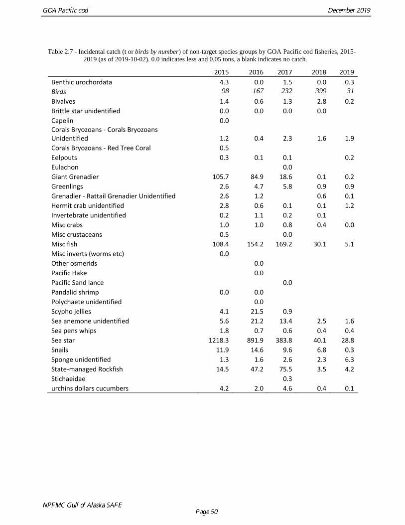
Table 2.7 - Incidental catch (t or birds by number) of non-target species groups by GOA Pacific cod fisheries, 2015-

2019 (as of 2019-10-02). 0.0 indicates less and 0.05 tons, a blank indicates no catch.

2015 2016 2017 2018 2019

Benthic urochordata 4.3 0.0 1.5 0.0 0.3

Birds 98 167 232 399 31

Bivalves 1.4 0.6 1.3 2.8 0.2

Brittle star unidentified 0.0 0.0 0.0 0.0 Capelin 0.0 Corals Bryozoans - Corals Bryozoans Unidentified 1.2 0.4 2.3 1.6 1.9

Corals Bryozoans - Red Tree Coral 0.5

Eelpouts 0.3 0.1 0.1 0.2

Eulachon 0.0

Giant Grenadier 105.7 84.9 18.6 0.1 0.2

Greenlings 2.6 4.7 5.8 0.9 0.9

Grenadier - Rattail Grenadier Unidentified 2.6 1.2 0.6 0.1

Hermit crab unidentified 2.8 0.6 0.1 0.1 1.2

Invertebrate unidentified 0.2 1.1 0.2 0.1 Misc crabs 1.0 1.0 0.8 0.4 0.0

Misc crustaceans 0.5 0.0

Misc fish 108.4 154.2 169.2 30.1 5.1

Misc inverts (worms etc) 0.0

Other osmerids 0.0

Pacific Hake 0.0

Pacific Sand lance 0.0

Pandalid shrimp 0.0 0.0

Polychaete unidentified 0.0

Scypho jellies 4.1 21.5 0.9

Sea anemone unidentified 5.6 21.2 13.4 2.5 1.6

Sea pens whips 1.8 0.7 0.6 0.4 0.4

Sea star 1218.3 891.9 383.8 40.1 28.8

Snails 11.9 14.6 9.6 6.8 0.3

Sponge unidentified 1.3 1.6 2.6 2.3 6.3

State-managed Rockfish 14.5 47.2 75.5 3.5 4.2

Stichaeidae 0.3

urchins dollars cucumbers 4.2 2.0 4.6 0.4 0.1

Table 2.8 – Pacific cod catch (t) by trip target in Gulf of Alaska groundfish fisheries. *Data for 2019 is as of

10/02/2019.

Trip Target 2015 2016 2017 2018 2019

Arrowtooth Flounder

1,384

1,346

1,266 960 1,302

Atka Mackerel -

10

5 12 -

Deep Water Flatfish - GOA - - - - -

Flathead Sole

1

39

2

2

18

Halibut

541

325

368

430

185

Other Species

12 -

2

1 -

Pacific Cod 74,052 60,789 46,008

12,461

10,691

Pollock - bottom

1,090

624

557

536

376

Pollock - midwater

622

230

55

64

58

Rex Sole - GOA

162

25

6

79

62

Rockfish

786

366

253

394

296

Sablefish

127

108

88

44

55

Shallow Water Flatfish - GOA

711

225

123

262

330

TOTAL 79,489 64,087 48,734 15,247 13,373

Non Pacific cod trip target total 5,437 3,297 2,726 2,786 2,682

Table 2.9 – Noncommercial fishery catch (in kg); total source amounts less than 1 kg were omitted (AFSC for GOA

bottom trawl survey values; AKFIN for other values, as of 2019-10-09)

Source 2014 2015 2016 2017

AFSC Annual Longline Survey 33,370 39,824 24,240 15,598

Bait for Crab Fishery 7,348 1,616 2,006 988

GOA Shelf and Slope Walleye Pollock Acoustic-Trawl Survey

53

Gulf of Alaska Bottom Trawl Survey

18,945

5,197

IPHC Annual Longline Survey 138,091 77,044 46,273 38,927

Kachemak Bay Large Mesh Trawl Survey

1,254

Kenai/Prince William Sound Walleye Pollock Acoustic-Trawl Survey

15

Kodiak Scallop Dredge

1

Large-Mesh Trawl Survey 13,090 8,072 6,076 6,597

Prince William Sound Large Mesh Trawl Survey

164

Salmon EFP 13-01 8,316

Scallop Dredge Survey

Shumagin Islands Walleye Pollock Acoustic-Trawl Survey

11

Small-Mesh Trawl Survey 1,424 1,412 160 161

Sport Fishery 199,263 183,813 122,501

Spot Shrimp Survey 12 10 2

Total 400,913 330,736 201,257 68,966

Table 2.10 – Pacific cod abundance measured in biomass (t) and numbers of fish (1000s), as assessed by the GOA

bottom trawl survey. Point estimates are shown along with coefficients of variation.

Year Biomass(t) CV Abundance CV

1984 550,971 0.096 320,525 0.102

1987 394,987 0.085 247,020 0.121

1990 416,788 0.100 212,132 0.135

1993 409,848 0.117 231,963 0.124

1996 538,154 0.131 319,068 0.140

1999 306,413 0.083 166,584 0.074

2001 257,614 0.133 158,424 0.118

2003 297,402 0.098 159,749 0.085

2005 308,175 0.170 139,895 0.135

2007 232,035 0.091 192,306 0.114

2009 752,651 0.195 573,469 0.185

2011 500,975 0.089 348,060 0.116

2013 506,362 0.097 337,992 0.099

2015 253,694 0.069 196,334 0.079

2017 107,342 0.128 56,199 0.117

2019 181,581 0.218 127,188 0.243

Table 2.11 – ABL Longline Relative Population Numbers (RPNs) and CVs for Pacific cod.

Year RPN CV Year RPN CV

1990 116,398 0.139 2007 34,992 0.140

1991 110,036 0.141 2008 26,881 0.228

1992 136,311 0.087 2009 68,391 0.138

1993 153,894 0.114 2010 86,722 0.138

1994 96,532 0.094 2011 93,732 0.141

1995 120,700 0.100 2012 63,749 0.148

1996 84,530 0.141 2013 48,534 0.162

1997 104,610 0.169 2014 69,653 0.143

1998 125,846 0.115 2015 88,410 0.160

1999 91,407 0.113 2016 83,887 0.172

2000 54,310 0.145 2017 39,523 0.101

2001 33,841 0.181 2018 23,853 0.121

2002 51,900 0.170 2019 14,933 0.185

2003 59,952 0.150

2004 53,108 0.118

2005 29,864 0.214

2006 34,316 0.197

Table 2.12 – IPHC Longline Relative Population Numbers (RPNs) and CVs for Pacific cod.

Year RPN CV Year RPN CV

1997 29,431.29 0.24

1998 16,389.47 0.20 2009 30,228.94 0.16

1999 12,387.02 0.21 2010 27,836.75 0.16

2000 14,599.59 0.22 2011 31,728.38 0.15

2001 12,192.47 0.23 2012 23,604.72 0.17

2002 16,372.69 0.21 2013 26,333.14 0.18

2003 15,361.62 0.22 2014 27,789.64 0.16

2004 16,075.93 0.20 2015 16,853.72 0.20

2005 16,397.51 0.23 2016 11,888.02 0.23

2006 15,761.12 0.20 2017 10,241.65 0.23

2007 18,196.23 0.19 2018 13,198.32 0.16

2008 22,201.86 0.17 2019 14,238.55 0.25

Table 2.13 – ADFG trawl survey deltaGLM biomass index and CVs for Pacific cod.

Year Index CV Year Index CV

1988 2.80 0.09 2005 1.06 0.09

1989 3.72 0.09 2006 0.91 0.09

1990 2.77 0.08 2007 1.09 0.08

1991 1.89 0.14 2008 1.26 0.07

1992 2.88 0.08 2009 1.26 0.07

1993 2.33 0.09 2010 1.07 0.07

1994 2.09 0.08 2011 1.37 0.07

1995 2.31 0.11 2012 2.60 0.09

1996 2.34 0.09 2013 1.96 0.10

1997 2.52 0.08 2014 1.35 0.10

1998 2.27 0.09 2015 1.22 0.10

1999 1.26 0.07 2016 0.84 0.11

2000 0.98 0.08 2017 0.89 0.11

2001 0.86 0.08 2018 1.16 0.10

2002 1.09 0.07 2019 0.97 0.09

2003 0.87 0.08

2004 1.34 0.07

Table 2.14 – CFSR bottom temperature index for 10 cm and 40 cm Pacific cod and Hobday (2018) marine heatwave

intensity index (MHWI) in °C days for full year and for winter for 1979-2019. Note that the MHWI

for 2019 are only through October 30.

Year 10cm 40cm

Annual

MHWI

Winter

MHWI Year 10cm 40cm

Annual

MHWI

Winter

MHWI

1979 4.91 4.70 0 0 1999 4.43 4.38 0 0

1980 5.03 4.74 0 0 2000 4.51 4.43 0 0

1981 5.71 5.20 0 0 2001 4.98 4.80 35.52 18.66

1982 4.00 4.08 0 0 2002 4.20 4.10 50.34 50.34

1983 5.11 4.87 24.82 24.82 2003 5.30 5.15 201.08 158.99

1984 4.73 4.75 75.56 41.44 2004 4.60 4.58 115.59 0

1985 4.57 4.58 22.2 22.2 2005 4.91 4.89 276.54 9.96

1986 4.73 4.53 15.67 15.67 2006 4.63 4.57 35.03 5.97

1987 5.30 5.00 5.45 5.45 2007 4.13 3.85 0 0

1988 4.70 4.60 0 0 2008 4.33 4.17 0 0

1989 4.05 3.95 0 0 2009 3.66 3.81 0 0

1990 4.12 4.11 8.56 0 2010 5.21 4.78 6.54 0

1991 4.38 4.26 0 0 2011 4.55 4.27 0 0

1992 4.89 4.60 0 0 2012 4.00 3.64 0 0

1993 4.52 4.37 19.02 0 2013 4.18 4.14 0 0

1994 4.47 4.46 0 0 2014 4.73 4.62 257.74 104.06

1995 4.04 4.04 0 0 2015 5.88 5.42 378.87 234.5

1996 4.50 4.40 0 0 2016 5.71 4.99 632.81 368.28

1997 4.56 4.46 138.58 24.12 2017 4.75 4.42 39.27 27.44

1998 5.73 5.20 152.42 152.42 2018 5.10 4.79 93.68 69.59

2019 5.94 5.46 368.06 144.65

Table 2.15 – Number of parameters by category for model configurations presented.

M18.10.44 M19.11.44 M19.14.48c

Recruitment

Early Init Ages 10 10 10

Early Rec. Devs

(1977)

1 1 1

Main Rec. Devs

(1978-2014)

37 37 37

Late Rec. Devs

(2015-2018)

5 4 4

Future Rec. Devs.

(2019-2023)

5 5 5

R0 1 1 1

1976 R reg. 1 1 1

Natural mortality 2 2 2

Growth 5 5 5

Aging Bias 0 0 2

Catchability

Qtrawl 1 1 1

Qlongline 1 1 1

Qlongline env. offset 1 1 1

Initial F 2 2 2

Selectivity

Trawl Survey 16 16 16

Longline survey 5 5 5

Trawl Fishery 58(39 dev) 58(39 dev) 58(39 dev)

Longline Fishery 39 (24 dev) 39 (24 dev) 39(24 dev)

Pot Fishery 8 8 8

Total 198 198 200

Table 2.16 – Model fit statistics and results. Note that likelihoods between model series are not completely

comparable. Note 2019 SSB is beginning of year from Stock Synthesis, 2020 and 2021 SSB are March

estimates from projection model assuming 6,300 t catch. Authors’ preferred model in green.

M18.10.44 M19.11.44 M19.14.48c

Likelihoods Total 2297.59 2349.20 2714.86

Survey -9.59 -11.79 -11.38

Length Comp. 1337.18 1342.63 1360.43

Age Comp. 963.36 1013.33 1362.03

Recruitment -6.34 -8.04 -9.00

Parameter priors 1.58 1.19 1.18

Parameter Devs. 5.83 6.09 6.10

Parameters

R0 billions 0.598 0.571 0.579

Steepness 1.0 1.0 1.0

Natural Mortality 0.49 0.49 0.49

M14-16 0.85 0.81 0.81

qShelf 1.16 1.10 1.08

qlongline 1.23 1.16 1.15

Lmin 5.29 3.49 2.3

Lmax 99.46 99.46 99.46

Von Bert K 0.17 0.18 0.19

Results

SSB1978 (t) 118,283 115,078 117,113

SSB100% (t) 173,544 185,651 187,780

SSB2019 (t) 29,386 32,387 33,274

SSB2019% 16.9 17.4 17.7

SSB2020(t) 29,782 31,840 32,958

SSB2020% 17.2 17.2 17.6

SSB2021(t) 38,841 40,403 42,026

SSB2021% 22.4 21.8 22.4

F35% 0.750 0.676 0.668

F40% 0.603 0.546 0.540

2020 ABC (t) 14,838 14,042 14,620

FABC 0.240 0.218 0.221

OFL (t) 18,168 17,104 17,794

FOFL 0.299 0.269 0.274

2021 ABC (t) 26,003 23,541 24,820

FABC 0.323 0.284 0.290

OFL (t) 31,705 28,574 30,099

FOFL 0.402 0.351 0.359

Table 2.17 – Likelihood components by fleet for all proposed models.

Model Label ALL FshTrawl FshLL FshPot Srv LLSrv

18.10.44 Age_like 963.36 258.38 264.82 210.90 229.27

19.11.44 Age_like 1013.33 238.86 289.10 210.25 275.12

19.14.48c Age_like 1362.03 241.02 287.31 208.83 624.87

18.10.44 Catch_like 4.38E-12 1.50E-12 1.48E-12 1.41E-12

19.11.44 Catch_like 6.93E-12 2.33E-12 2.34E-12 2.26E-12

19.14.48c Catch_like 8.14E-12 2.73E-12 2.76E-12 2.66E-12

18.10.44 Length_like 1337.18 393.66 289.72 291.74 144.13 217.94

19.11.44 Length_like 1342.63 397.32 284.38 290.74 153.93 216.25

19.14.48c Length_like 1360.43 401.11 283.24 291.45 166.75 217.87

18.10.44 Surv_like -9.60 -10.56 0.96

19.11.44 Surv_like -11.79 -11.87 0.08

19.14.48c Surv_like -11.38 -11.80 0.42

Table 2.18 – Retrospective analysis, index RMSE, harmonic mean effective N for length and age compositions, and

recruitment variability for selected assessed models.

M18.10.44 M19.11.44 M19.14.48c

Retrospective

Spawning biomass Mohn’s ρ 0.182 0.155 0.118

Woods Hole ρ 0.190 0.177 0.148

RMSE 0.195 0.185 0.174

Recruit. (age -0) Mohn’s ρ 0.347 0.246 0.197

Woods Hole ρ 0.338 0.295 0.217

RMSE 0.307 0.276 0.233 Index RMSE

AFSC Trawl 0.290 0.277 0.277

AFSC Longline 0.316 0.317 0.318

Size Comp

Har. Mean EffN Trawl 313.60 309.88 308.61.

Longline 451.69 452.49 454.03

Pot 414.64 416.45 413.66

AFSC Trawl 327.37 313.64 305.71

AFSC Longline 283.86 286.84 285.13

Mean input N Trawl 147.45 147.45 147.45

Longline 155.13 155.13 155.13

Pot 171.00 171.00 171.00

AFSC Trawl 94.38 94.38 94.38

AFSC Longline 100.00 100.00 100.00

Age Data

Har. Mean EffN Trawl 1.64 1.84 1.81

Longline 2.67 2.69 2.68

Pot 2.35 2.53 2.51

AFSC Trawl 2.81 2.90 2.93

Mean input N Trawl 1.03 1.03 1.03

Longline 1.59 1.59 1.59

Pot 1.23 1.23 1.23

AFSC Trawl 1.42 1.42 1.42

Rec. Var. (1977-2017)

Std.dev(ln(No. Age 1)) 0.55 0.52 0.51

Table 2.19 – Estimated beginning year weight and length at age from Model 19.14.48c.

Age Weight (kg) Length (cm)

0 1.35E-04 0.5

1 0.013 10.919

2 0.161 25.914

3 0.536 38.369

4 1.121 48.715

5 1.856 57.309

6 2.672 64.447

7 3.513 70.377

8 4.336 75.302

9 5.113 79.394

10 7.082 88.036

Table 2.20 – Estimated female spawning biomass (t) from the last year’s assessment and this year’s

assessment from Models 18.10.44 and the author’s recommended Model 19.14.48c.

Last Year's Model Model19.14.48c

Sp.Bio St.dev Tot. Bio. 0+ Sp.Bio St.dev Tot. Bio. 0+

1977 120,453 28,059 403,588 104,750 23,105 340,687

1978 130,267 29,204 422,439 117,115 24,505 353,530

1979 126,010 27,365 504,136 114,285 23,198 401,961

1980 123,733 25,682 593,197 110,135 21,309 465,619

1981 151,436 30,339 635,060 125,320 23,684 496,767

1982 188,497 36,725 668,967 153,290 28,367 524,234

1983 197,736 37,047 713,828 162,280 29,274 565,329

1984 200,333 35,954 758,519 164,770 28,964 612,364

1985 218,129 35,924 798,787 182,455 29,559 664,827

1986 242,500 35,204 837,433 210,695 29,955 715,967

1987 254,206 32,877 871,227 232,910 29,421 764,445

1988 255,330 29,508 873,994 236,290 26,653 778,122

1989 263,180 26,925 857,974 245,590 24,537 777,175

1990 260,761 23,944 823,846 248,915 22,288 759,213

1991 236,943 20,755 776,061 228,490 19,601 717,933

1992 215,133 18,336 743,411 210,315 17,628 689,490

1993 199,049 16,766 705,219 193,725 16,084 654,597

1994 200,625 15,889 667,998 196,020 15,306 627,867

1995 201,299 14,614 613,486 199,155 14,210 588,782

1996 180,727 12,558 533,819 179,380 12,250 518,686

1997 151,465 10,273 470,311 153,285 10,210 461,210

1998 122,877 8,463 418,822 127,445 8,561 413,127

1999 107,276 7,598 379,079 112,615 7,674 375,787

2000 95,443 7,154 338,390 100,450 7,173 335,702

2001 87,620 6,642 325,728 91,975 6,585 318,708

2002 82,855 6,079 334,660 87,065 5,971 324,404

2003 82,785 5,910 336,484 85,975 5,663 325,922

2004 85,552 6,116 317,059 87,350 5,736 307,850

2005 83,110 5,936 288,103 84,680 5,590 280,816

2006 76,069 5,264 272,454 77,450 4,995 264,538

2007 66,572 4,594 281,250 68,365 4,420 268,873

2008 59,467 4,316 316,237 61,215 4,161 299,342

2009 62,478 4,809 364,318 62,835 4,557 342,596

2010 81,083 6,076 421,953 81,485 5,743 401,264

2011 95,334 7,507 441,055 94,895 7,039 425,866

2012 105,408 8,952 442,457 105,105 8,484 428,225

2013 109,747 9,903 467,634 113,350 9,743 445,224

2014 109,814 10,778 541,959 113,830 10,614 498,565

2015 76,280 6,691 413,621 80,020 6,587 381,875

2016 60,085 5,033 278,457 62,215 4,811 257,969

2017 45,374 4,036 166,636 46,080 3,787 155,394

2018 39,723 4,208 146,433 37,369 3,837 127,165

2019 34,701 4,075 183,503 35,231 3,711 141,458

2020 33,274 170,124

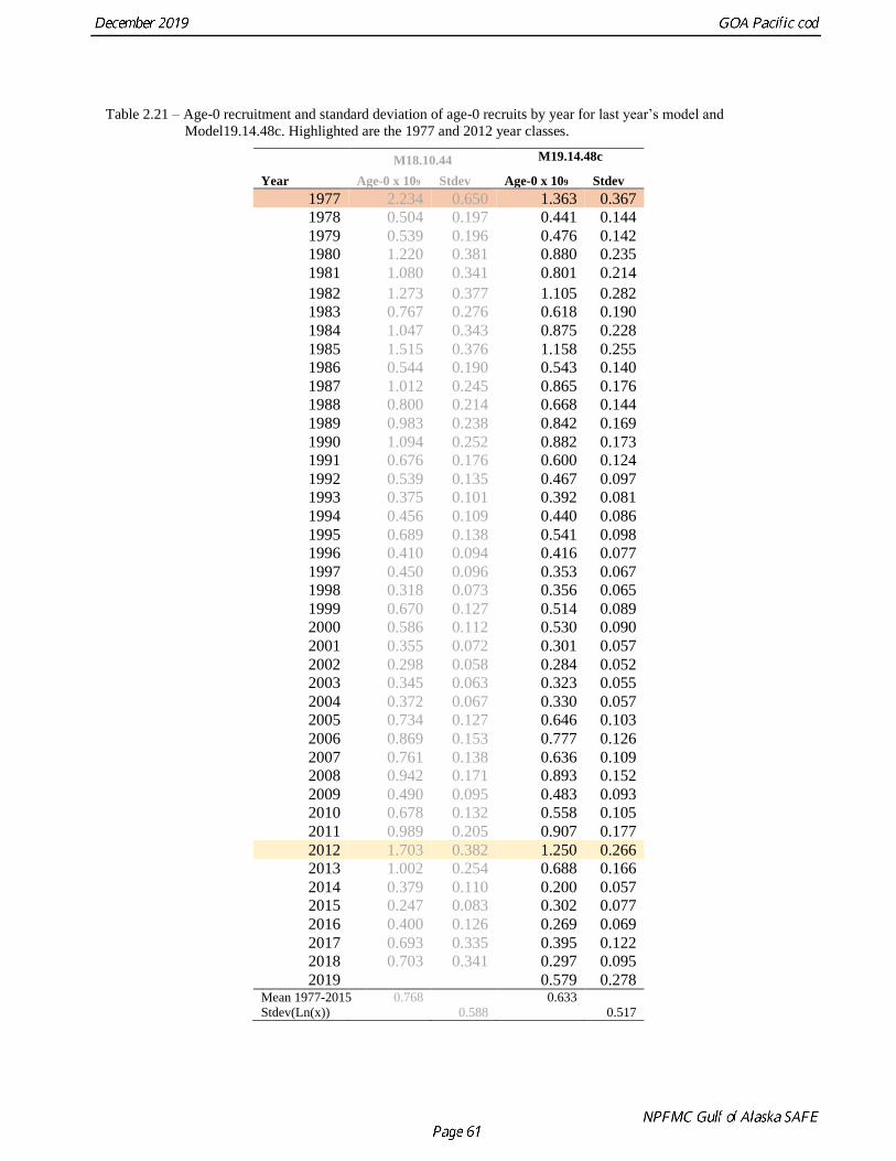
Table 2.21 – Age-0 recruitment and standard deviation of age-0 recruits by year for last year’s model and

Model19.14.48c. Highlighted are the 1977 and 2012 year classes.

M18.10.44 M19.14.48c

Year Age-0 x 109 Stdev Age-0 x 109 Stdev

1977 2.234 0.650 1.363 0.367

1978 0.504 0.197 0.441 0.144

1979 0.539 0.196 0.476 0.142

1980 1.220 0.381 0.880 0.235

1981 1.080 0.341 0.801 0.214

1982 1.273 0.377 1.105 0.282

1983 0.767 0.276 0.618 0.190

1984 1.047 0.343 0.875 0.228

1985 1.515 0.376 1.158 0.255

1986 0.544 0.190 0.543 0.140

1987 1.012 0.245 0.865 0.176

1988 0.800 0.214 0.668 0.144

1989 0.983 0.238 0.842 0.169

1990 1.094 0.252 0.882 0.173

1991 0.676 0.176 0.600 0.124

1992 0.539 0.135 0.467 0.097

1993 0.375 0.101 0.392 0.081

1994 0.456 0.109 0.440 0.086

1995 0.689 0.138 0.541 0.098

1996 0.410 0.094 0.416 0.077

1997 0.450 0.096 0.353 0.067

1998 0.318 0.073 0.356 0.065

1999 0.670 0.127 0.514 0.089

2000 0.586 0.112 0.530 0.090

2001 0.355 0.072 0.301 0.057

2002 0.298 0.058 0.284 0.052

2003 0.345 0.063 0.323 0.055

2004 0.372 0.067 0.330 0.057

2005 0.734 0.127 0.646 0.103

2006 0.869 0.153 0.777 0.126

2007 0.761 0.138 0.636 0.109

2008 0.942 0.171 0.893 0.152

2009 0.490 0.095 0.483 0.093

2010 0.678 0.132 0.558 0.105

2011 0.989 0.205 0.907 0.177

2012 1.703 0.382 1.250 0.266

2013 1.002 0.254 0.688 0.166

2014 0.379 0.110 0.200 0.057

2015 0.247 0.083 0.302 0.077

2016 0.400 0.126 0.269 0.069

2017 0.693 0.335 0.395 0.122

2018 0.703 0.341 0.297 0.095

2019 0.579 0.278 Mean 1977-2015 0.768 0.633

Stdev(Ln(x)) 0.588 0.517

Table 2.22 – Estimated fishing mortality in Apical F and Total exploitation for Model 19.14.48c.

Sum Apical F Total

Exploitation

Sum Apical F Total

Exploitation Year F σ Year F σ

1977 0.005 0.001 0.007 2001 0.087 0.007 0.147

1978 0.032 0.007 0.038 2002 0.078 0.007 0.146

1979 0.033 0.008 0.047 2003 0.094 0.008 0.172

1980 0.043 0.009 0.081 2004 0.124 0.010 0.197

1981 0.064 0.012 0.078 2005 0.111 0.009 0.184

1982 0.053 0.010 0.063 2006 0.114 0.009 0.200

1983 0.049 0.009 0.072 2007 0.139 0.011 0.234

1984 0.030 0.005 0.044 2008 0.122 0.010 0.239

1985 0.012 0.002 0.023 2009 0.093 0.008 0.179

1986 0.023 0.003 0.038 2010 0.136 0.011 0.228

1987 0.036 0.007 0.048 2011 0.121 0.011 0.218

1988 0.032 0.004 0.046 2012 0.129 0.012 0.201

1989 0.049 0.007 0.060 2013 0.120 0.012 0.180

1990 0.058 0.006 0.102 2014 0.136 0.015 0.203

1991 0.067 0.007 0.116 2015 0.149 0.015 0.227

1992 0.071 0.007 0.128 2016 0.205 0.018 0.256

1993 0.050 0.005 0.092 2017 0.288 0.028 0.338

1994 0.047 0.004 0.080 2018 0.089 0.011 0.136

1995 0.079 0.007 0.123 2019 0.059 0.008 0.103

1996 0.091 0.008 0.140

1997 0.098 0.008 0.161

1998 0.088 0.007 0.161

1999 0.113 0.009 0.195

2000 0.106 0.009 0.176

Table 2.23 – Model 19.14.48c parameters and reference estimates MLE and MCMC derived. SSB is calculated for

January 1 in this table. FSSB100% is female unfished spawning biomass from Stock Synthesis

calculated using 1977-2017 as reference.

MLE estimates MCMC posterior distribution

MLE σ 50% 2.5% 97.5%

MStandard 0.4886 0.0206 0.4819 0.4407 0.5214

M2014-2016 0.8121 0.0521 0.8003 0.6822 0.8968

Von Bert K 0.1855 0.0021 0.1847 0.1807 0.1891

Lmin 2.3115 0.5625 2.3999 1.3236 3.4925

Lmax 99.4614 0.0150 99.4617 99.4342 99.4881

Ln(QTrawl survey) 0.0799 0.0871 0.1112 -0.0552 0.2785

Ln(Qll survey) 0.1378 0.0704 0.1772 0.0602 0.3145

Ln(Qll survey envir.) 1.0829 0.0344 0.9263 0.5128 1.6020

FSSB1978 117,115 24,505 112,872 77,648 165,303

FSSB2019 35,231 3,711 33,803 27,940 40,690

Recr_1977 1,363,400 366,770 1,293,625 758,904 2,147,373

Recr_2012 1,250,100 265,600 1,177,775 767,083 1,740,844

FSSB100% 172,629 13,459 170,420 148,490 197,715

FSSB2019/FSSB100% 20.4% 19.8% 16.2% 24.2%

Table 2.24 – Biological reference points from GOA Pacific cod SAFE documents for years 2001 – 2019

Year SB100% SB40% F40% SBy+1 ABCy+1

2001 212,000 85,000 0.41 82,000 57,600

2002 226,000 90,300 0.35 88,300 52,800

2003 222,000 88,900 0.34 103,000 62,810

2004 211,000 84,400 0.31 91,700 58,100

2005 329,000 132,000 0.56 165,000 68,859

2006 259,000 103,000 0.46 136,000 68,859

2007 302,000 121,000 0.49 108,000 66,493

2008 255,500 102,200 0.52 88,000 55,300

2009 291,500 116,600 0.49 117,600 79,100

2010 256,300 102,500 0.42 124,100 86,800

2011 261,000 104,000 0.44 121,000 87,600

2012 234,800 93,900 0.49 111,000 80,800

2013 227,800 91,100 0.54 120,100 88,500

2014 316,500 126,600 0.50 155,400 102,850

2015 325,200 130,000 0.41 116,600 98,600

2016 196,776 78,711 0.53 105,378 88,342

2017 168,583 67,433 0.80 35,973 18,972

2018 172,240 68,896 0.76 34,515 19,665

2019 187,780 75,112 0.67 32,957 14,621

Table 2.25 – Number of fish at age-1 from Model 19.14.48c with the M 2014-2016 block fixed at the standard M

value used in projection model.

Year Age-1 Year Age-1

1977 236,700 2000 317,328

1978 836,739 2001 328,025

1979 270,550 2002 187,192

1980 292,016 2003 176,125

1981 540,089 2004 198,647

1982 491,871 2005 196,316

1983 678,677 2006 376,135

1984 379,600 2007 428,542

1985 538,300 2008 338,917

1986 712,027 2009 428,897

1987 331,248 2010 206,826

1988 528,906 2011 210,410

1989 408,224 2012 283,787

1990 515,772 2013 331,254

1991 539,478 2014 161,998

1992 368,156 2015 51,013

1993 286,643 2016 101,296

1994 240,666 2017 109,078

1995 270,246

1996 332,461

1997 256,198

1998 216,840

1999 219,211

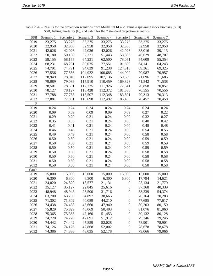
Table 2.26 – Results for the projection scenarios from Model 19.14.48c. Female spawning stock biomass (SSB)

SSB, fishing mortality (F), and catch for the 7 standard projection scenarios.

SSB Scenario 1 Scenario 2 Scenario 3 Scenario 4 Scenario 5 Scenario 6 Scenario 7

2019 33,275 33,275 33,275 33,275 33,275 33,275 33,275

2020 32,958 32,958 32,958 32,958 32,958 32,958 32,958

2021 42,026 42,026 42,026 42,026 42,026 38,016 39,113

2022 50,180 50,180 52,321 51,443 58,806 46,629 48,707

2023 58,155 58,155 64,231 62,500 78,051 54,609 55,354

2024 68,231 68,231 80,075 77,551 101,500 64,141 64,243

2025 74,791 74,791 94,639 91,238 124,818 69,361 69,325

2026 77,556 77,556 104,922 100,685 144,009 70,987 70,957

2027 78,949 78,949 112,095 107,136 159,659 71,696 71,685

2028 79,089 79,089 115,910 110,459 169,823 71,542 71,538

2029 78,501 78,501 117,775 111,926 177,341 70,858 70,857

2030 78,127 78,127 118,428 112,372 181,586 70,555 70,556

2031 77,788 77,788 118,507 112,348 183,891 70,313 70,313

2032 77,881 77,881 118,698 112,492 185,435 70,457 70,458 F

2019 0.24 0.24 0.24 0.24 0.24 0.24 0.24

2020 0.09 0.09 0.09 0.09 0.09 0.27 0.22

2021 0.29 0.29 0.21 0.24 0.00 0.32 0.27

2022 0.35 0.35 0.21 0.24 0.00 0.40 0.42

2023 0.41 0.41 0.21 0.24 0.00 0.48 0.48

2024 0.46 0.46 0.21 0.24 0.00 0.54 0.55

2025 0.49 0.49 0.21 0.24 0.00 0.58 0.58

2026 0.50 0.50 0.21 0.24 0.00 0.59 0.59

2027 0.50 0.50 0.21 0.24 0.00 0.59 0.59

2028 0.50 0.50 0.21 0.24 0.00 0.59 0.59

2029 0.50 0.50 0.21 0.24 0.00 0.58 0.58

2030 0.50 0.50 0.21 0.24 0.00 0.58 0.58

2031 0.50 0.50 0.21 0.24 0.00 0.58 0.58

2032 0.50 0.50 0.21 0.24 0.00 0.58 0.58

Catch

2019 15,000 15,000 15,000 15,000 15,000 15,000 15,000

2020 6,300 6,300 6,300 6,300 6,300 17,794 14,621

2021 24,820 24,820 18,577 21,131 0 25,134 21,779

2022 35,127 35,127 22,845 25,616 0 37,368 40,339

2023 48,948 48,948 28,500 31,716 0 53,239 54,374

2024 63,700 63,700 34,897 38,665 0 70,164 70,283

2025 71,302 71,302 40,089 44,210 0 77,685 77,617

2026 74,438 74,438 43,660 47,940 0 80,203 80,159

2027 75,829 75,829 46,069 50,403 0 81,076 81,060

2028 75,365 75,365 47,160 51,453 0 80,132 80,128

2029 74,720 74,720 47,691 51,912 0 79,246 79,246

2030 74,442 74,442 47,859 52,028 0 78,901 78,901

2031 74,126 74,126 47,868 52,002 0 78,678 78,678

2032 74,386 74,386 48,035 52,178 0 79,066 79,066

Table 2.27 – Gulf of Alaska Pacific cod catch and ex-vessel data. Total and retained catch (thousand

metric tons), ex-vessel value (million US$) and price (US$ per pound), hook and line and pot gear share

of catch, inshore sector share of catch, number of vessel; 2009-2013 average and 2014-2018.

Source: NMFS Alaska Region Blend and Catch-accounting System estimates; NMFS Alaska Region At-sea

Production Reports; and ADF&G Commercial Operators Annual Reports (COAR). Data compiled and provided by

the Alaska Fisheries Information Network (AKFIN).

Table 2.28 – Gulf of Alaska Pacific cod first-wholesale market data. First-wholesale production (thousand

metric tons), value (million US$), price (US$ per pound), fillet and head and gut volume (thousand metric

tons), value share, and price (US$ per pound), inshore share of value; 2009-2013 average and 2014-2018.

Source: NMFS Alaska Region Blend and Catch-accounting System estimates; NMFS Alaska Region At-sea

Production Reports; and ADF&G Commercial Operators Annual Reports (COAR). Data compiled and provided by

the Alaska Fisheries Information Network (AKFIN).

Avg 09-13 2014 2015 2016 2017 2018

Total catch K mt 72.7 84.9 79.5 64.1 48.7 15.2

Retained catch K mt 69.7 79.5 77.5 63.1 48.0 14.4

Ex-vessel value M $ $46.7 $52.1 $50.3 $41.0 $35.3 $14.5

Ex-vessel price lb $ $0.304 $0.297 $0.293 $0.294 $0.334 $0.452

Hook & line share of catch 27% 23% 21% 17% 18% 23%

Pot gear share of catch 49% 48% 52% 60% 55% 53%

Central Gulf share of catch 61% 59% 60% 53% 43% 47%

Shoreside share of catch 89% 91% 92% 92% 87% 88%

Vessels # 432.6 341 382 358 246 151

Avg 09-13 2014 2015 2016 2017 2018

All Products volume K mt 29.11 31.07 32.00 21.65 17.39 5.58

All Products value M $ $102.0 $118.0 $102.5 $91.8 $75.5 $32.0

All Products price lb $ $1.59 $1.72 $1.45 $1.92 $1.97 $2.60

Fillets volume K mt 8.79 9.85 6.39 7.87 6.52 2.00

Fillets value share 54.8% 57.1% 36.3% 62.4% 60.0% 60.0%

Fillets price lb $ $2.88 $3.10 $2.64 $3.30 $3.15 $4.35

Head & Gut volume K mt 12.15 13.95 19.05 8.43 6.11 1.92

Head & Gut value share 31.8% 32.5% 50.9% 24.7% 26.9% 27.2%

Head & Gut price lb $ $1.21 $1.25 $1.24 $1.22 $1.51 $2.05

Table 2.29 Cod U.S. trade and global market data. Global production (thousand metric tons), U.S. share

of global production, and Europe’s share of global production; U.S. export volume (thousand metric

tons), value (million US$), and price (US$ per pound); U.S. cod consumption (estimated), and share of

domestic production remaining in the U.S. (estimated); and the share of U.S. export volume and value for

head and gut (H&G), fillets, China, Japan, and Germany and Netherlands; 2009-2013 average and 2014-

2019.

Notes: Pacific cod in this table is for all U.S. Unless noted, `cod’ in this table refers to Atlantic and

Pacific cod. Russia, Norway, and Iceland account for the majority of Europe’s cod catch which is largely

focused in the Barents sea.

*Europe export statistics refers to: Austria, Belgium, Denmark, France, Germany, Greece, Ireland, Italy,

Netherlands, Norway, Portugal, Spain, Sweden, Switzerland, and United Kingdom Source: FAO Fisheries & Aquaculture Dept. Statistics http://www.fao.org/fishery/statistics/en. NOAA Fisheries,

Fisheries Statistics Division, Foreign Trade Division of the U.S. Census Bureau,

http://www.st.nmfs.noaa.gov/commercial-fisheries/foreign-trade/index. U.S. Department of Agriculture

http://www.ers.usda.gov/data-products/agricultural-exchange-rate-data-set.aspx.

Avg 09-13 2014 2015 2016 2017 2018

2019

(thru June)

1,506 1,852 1,762 1,792 1,759 - -

18.6% 17.6% 18.0% 17.9% 17.0% - -

74.2% 75.9% 74.8% 74.8% 75.7% - -

Pacific cod share of U.S. catch 97.8% 99.3% 99.5% 99.5% 99.7% - -

U.S. cod consumption K mt (est.) 88 115 108 114 119 113 -

Share of U.S. cod not exported 27% 31% 26% 29% 32% 35% -

98.3 107.3 113.2 105.3 92.8 73.2 39.4

$309.9 $314.2 $335.0 $312.0 $295.5 $253.6 $133.6

$1.429 $1.328 $1.342 $1.344 $1.445 $1.570 $1.539

volume Share 74% 92% 91% 94% 94% 91% 90%

value share 74% 91% 90% 92% 92% 90% 89%

volume Share 10% 2% 3% 3% 4% 5% 6%

value share 12% 4% 4% 4% 5% 6% 6%

volume Share 39% 54% 53% 55% 52% 47% 47%

value share 37% 51% 51% 52% 50% 46% 45%

volume Share 17% 16% 13% 14% 16% 15% 7%

value share 18% 16% 14% 15% 18% 17% 8%

volume Share 30% 20% 19% 17% 17% 16% 20%

value share 32% 22% 19% 18% 18% 18% 21%

Global cod catch K mt

U.S. P. cod share of global catch

Europe share of global catch

Export volume K mt

Frozen

(H&G)

Fillets

China

Japan

Europe*

Export value M US$

Export price lb US$

Figures

Figure 2.1 Gulf of Alaska mean lengths with climate reconstruction. The shaded boxes represent periods of

significant changes in air temperature, sea surface temperature, storminess, and ocean circulation that

drive ocean productivity. The lightly shaded boxes represent periods of cooler and stormier

environments, which are generally more productive, while the darkly shaded boxes represent warmer

and generally less productive environments. Dates are presented as calibrated means; (From Betts et

al. 2011; Figure 11.4).

Figure 2.2 Tag recoveries from Shimada and Kimura 1994 (Figure 8), showing movement of individual tagged

Pacific cod from eastern Bering Sea into the Gulf of Alaska and other interregional migrations.

Figure 2.3 Discriminant analysis of principal components (DAPC) scatterplot with the following populations represented: Adak (2006), Prince William

Sound, PWS (2012), Kodiak (2003), Unimak (2018), Pervenets (2016), Pribilof (2017), and Norton Sound, NBS (2017). All populations represent

spawning groups except the Norton Sound sample, which was sampled in August, 2017. Note: The Norton Sound sample in panel b. is behind the

Unimak and Pribilof labels, and barely visible.

Figure 2.4. Pacific cod larval abundance from late spring ichthyoplankton surveys in the Gulf of Alaska using all

stations within a core area covering the Shelikof Sea valley and Semidi bank area.

Figure 2.5 Log larval area weighted CPUE from late spring ichthyoplankton surveys in the Gulf of Alaska using

all stations within a core area covering the Shelikof Sea valley and Semidi bank area by mean annual

temperature at 48m bottom depth in the Central GOA from the CFSR reanalysis data.

CF

SR

0-2

0 c

m P

acif

ic c

od t

emper

ature

anom

aly °

C

Figure 2.6 Abundance (catch per set, where present) of age-0 cod in beach seines, summer (left) 2018 and right

(2019). Each point plots the average abundance for a given bay, with 4-16 individual sets within each

bay.

Figure 2.7 Index of the sum of the annual marine heatwave cumulative intensity (℃ days) for 1981-2019 (larger

yellow points) and index of the sum of the annual winter marine heatwave cumulative intensity for

1981-2019 (smaller blue points) from the daily mean sea surface temperatures NOAA high resolution

blended analysis data for the Central Gulf of Alaska. The 2019 index value is the sum through 30

October 2019.

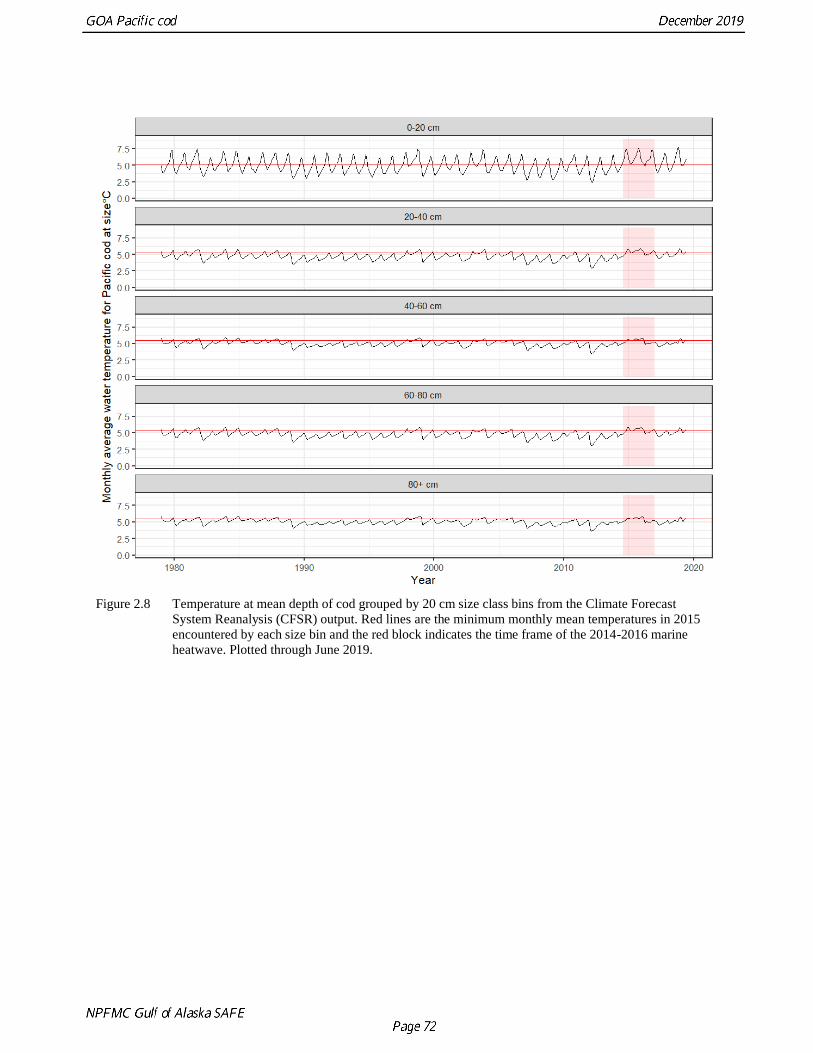
Figure 2.8 Temperature at mean depth of cod grouped by 20 cm size class bins from the Climate Forecast

System Reanalysis (CFSR) output. Red lines are the minimum monthly mean temperatures in 2015

encountered by each size bin and the red block indicates the time frame of the 2014-2016 marine

heatwave. Plotted through June 2019.

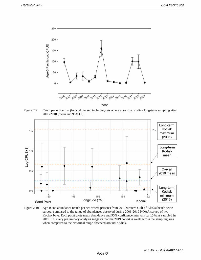
Figure 2.9 Catch per unit effort (log cod per set, including sets where absent) at Kodiak long-term sampling sites,

2006-2018 (mean and 95% CI).

Figure 2.10 Age-0 cod abundance (catch per set, where present) from 2019 western Gulf of Alaska beach seine

survey, compared to the range of abundances observed during 2006-2019 NOAA survey of two

Kodiak bays. Each point plots mean abundance and 95% confidence intervals for 15 bays sampled in

2019. This very preliminary analysis suggests that the 2019 cohort is weak across the sampling area

when compared to the historical range observed around Kodiak.

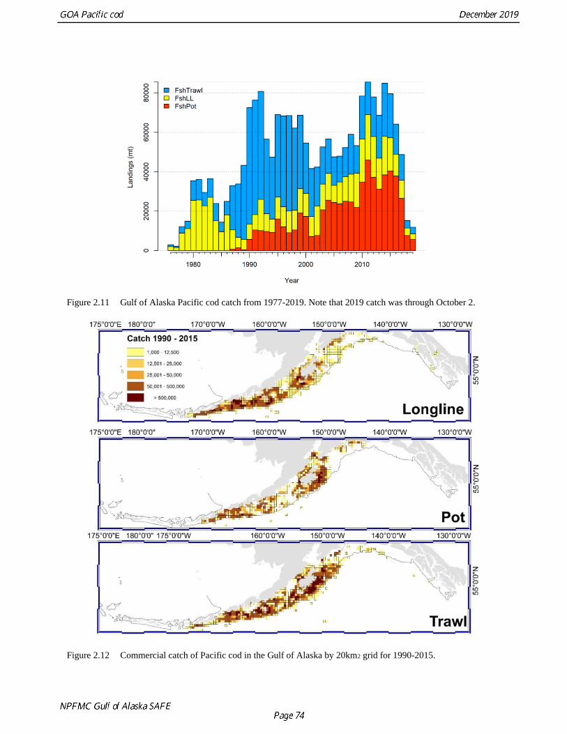
Figure 2.11 Gulf of Alaska Pacific cod catch from 1977-2019. Note that 2019 catch was through October 2.

Figure 2.12 Commercial catch of Pacific cod in the Gulf of Alaska by 20km2 grid for 1990-2015.

Figure 2.13 Commercial catch of Pacific cod in the Gulf of Alaska by 20km2 grid for 2018 for catch greater than

1000 kg.

Figure 2.14 Commercial catch of Pacific cod in the Gulf of Alaska by 20km2 grid for 2019 as of October 28, 2019

for catch greater than 1000 kg.

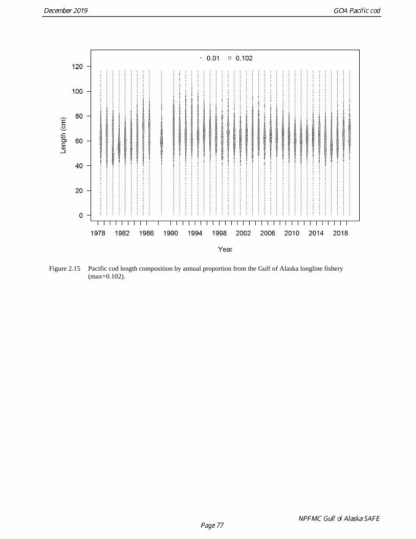
Figure 2.15 Pacific cod length composition by annual proportion from the Gulf of Alaska longline fishery

(max=0.102).

Figure 2.16 Mean length (cm) of Pacific cod from the Gulf of Alaska longline fishery.

Figure 2.17 Pacific cod length composition by annual proportion from the Gulf of Alaska pot fishery (max=0.1).

Figure 2.18 Mean length (cm) of Pacific cod from the Gulf of Alaska pot fishery.

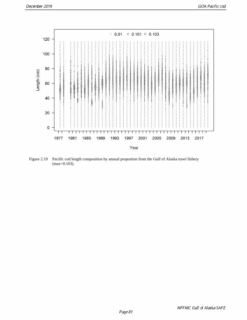
Figure 2.19 Pacific cod length composition by annual proportion from the Gulf of Alaska trawl fishery

(max=0.103).

Figure 2.20 Mean length (cm) of Pacific cod from the Gulf of Alaska trawl fishery.

Figure 2.21 Cumulative catch by week of the year and gear for 2015-2019 in the Central regulatory area. 2019

data are through October 10, 2019.

Figure 2.22 Cumulative catch by week of the year and gear for 2015-2019 in the Western regulatory area. The

2019 data are through October 10, 2019.

Figure 2.23 Boxplot of CPUE by number from the 2008-2019 Pacific cod CPUE for January-April for the Central (top) and Western (bottom) regulatory areas.

Note that the data in these figures are not controlled for vessel or gear differences within a gear type across time, but shows the raw CPUE data

distribution. These represent all catches and is limited to the directed cod fishery.

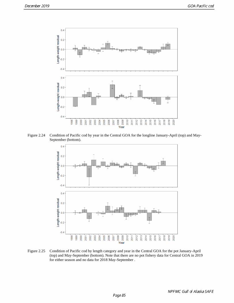
Figure 2.24 Condition of Pacific cod by year in the Central GOA for the longline January-April (top) and May-

September (bottom).

Figure 2.25 Condition of Pacific cod by length category and year in the Central GOA for the pot January-April

(top) and May-September (bottom). Note that there are no pot fishery data for Central GOA in 2019

for either season and no data for 2018 May-September .

Figure 2.26 Condition of Pacific cod by year in the Western GOA for the longline January-April (top) and May-

September (bottom).

Figure 2.27 Condition of Pacific cod by year in the Western GOA for pot January-April (top) and May-September

(bottom).

Figure 2.28 Proportion of pelagic trawls in the A Season (January-April) walleye pollock fishery with Pacific cod

present by region.

Figure 2.29 Pacific cod bycatch in the Gulf of Alaska shallow water flatfish fishery as tons of Pacific cod per tons

of total catch in the fishery by year.

Figure 2.30 GOA bottom trawl survey abundance (numbers) estimate. Bars and shading indicate the 95th percentile confidence intervals.

Figure 2.31 GOA bottom trawl survey Pacific cod population numbers at length estimates (max = 0.07).

Figure 2.32 Mean length (cm) of Pacific cod in the GOA bottom trawl survey.

Figure 2.33 Distribution of AFSC bottom trawl survey CPUE of Pacific cod for 2015-2019.

Figure 2.34 AFSC longline survey Pacific cod relative population numbers (RPN) time series. Bars and shading

indicate the 95th percentile confidence intervals.

Figure 2.35 AFSC longline survey Pacific cod size composition (max=0.09).

Figure 2.36 Mean length (cm) of Pacific cod from the AFSC longline survey.

Figure 2.37 IPHC halibut longline survey Pacific cod RPN time series. Bars and shading indicate the 95th

percentile confidence intervals.

Figure 2.38 IPHC halibut longline survey Pacific cod RPN length composition collection for 2018 by NMFS

management area.

Figure 2.39 ADFG bottom trawl survey delta-glm Pacific cod density index time series. Bars and shading indicate

the 95th percentile confidence intervals.

Figure 2.40 ADFG large-mesh trawl survey Pacific cod population numbers at length estimates.

Figure 2.41 Climate Forcast System Reanalysis (CFSR) Central Gulf of Alaska bottom temperatures at the AFSC

bottom trawl survey mean depths for 0-20 cm and 40-60 cm Pacific cod in June.

Figure 2.42 Data used in the 2019 models, circle area is relative to initial precision within data type.

Trawl Longline Pot

Age

Figure 2.43 Pacific cod age composition data from the Gulf of Alaska fisheries by gear type.

Figure 2.44 Pacific cod conditional length at age from the Gulf of Alaska trawl fishery.

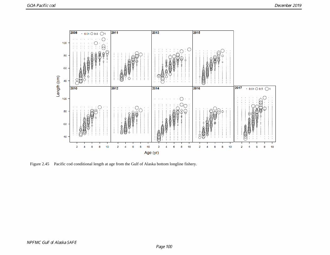
Figure 2.45 Pacific cod conditional length at age from the Gulf of Alaska bottom longline fishery.

Figure 2.46 Pacific cod conditional length at age from the Gulf of Alaska pot fishery.

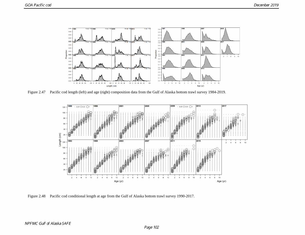
Figure 2.47 Pacific cod length (left) and age (right) composition data from the Gulf of Alaska bottom trawl survey 1984-2019.

Figure 2.48 Pacific cod conditional length at age from the Gulf of Alaska bottom trawl survey 1990-2017.

Figure 2.49 Length-at-age by year for each age 1 through 10 for Pacific cod otoliths collected during the summer bottom trawl surveys showing an increase in

median length in 2007 for ages 2 through 6.

Figure 2.50 Fit to von Bertalanffy growth model for 2007-2015 length at age data from the AFSC bottom trawl

surveys.

Figure 2.51 Bootstrapped (n=1000) parameters and results for the logistic length-based maturity using Stark

(2007) reread otolith and maturity data. Proportion mature 𝑷 = 𝟏𝟏 + 𝒆−(𝑨+𝑩𝑳)⁄ and L50 = A/-B

Fork

len

gth

(cm

)

Figure 2.52 (Left top) Aging error matrix from reader-tester validation with red line showing mean first read by

test read, (top right) as implemented in Model 19.14.48c with aging bias for pre-2007 age data. The red

line in this figure indicates the mean true age by observed age.

Figure 2.53 1977-2019 Gulf of Alaska Pacific cod female spawning biomass from the 2003 through 2019 stock assessments with the author’s preferred Model

19.14.48c as the 2019 estimate and (inset) images from the NMFS small net surveys off Kodiak Alaska showing change in species composition

over time from: http://www.thexxnakedscientists.com/HTML/articles/article/brucewrightcolumn1.htm/

Figure 2.54 Estimates of female spawning biomass (t; top) and age-0 recruits (billions; bottom) for 2018 reference

model without (Model 18.10.44), with 2019 data and change in plus age group to 10+ and aging error

(Model 19.11.44), and the proposed alternative 2019 model (Model19.14.48c) with pre-2007 age data

and aging bias.

Figure 2.55 Estimates of trawl fishery selectivity for Model 18.10.44, Model 19.11.44, and Model 19.14.48c. Red

dashed line is the size at 50% mature

Model19.11.44 Model18.10.44

Model19.14.48c

Figure 2.56 Model18.10.44, Model19.11.44, and Model19.14.48c selectivity for all size composition

components for 2019.

Model18.10.44 Model19.11.44

Model19.14.48c

Figure 2.57 Model fits to AFSC bottom trawl (left) and AFSC longline (right) survey indices.

Model18.10.44

Model19.11.44

Model19.14.48c

Figure 2.58 Estimates of fishery and AFSC bottom trawl survey selectivities for Model 18.10.44 (left) and Model

19.14.48c (right). Red dashed line is the size at 50% mature.

M18.10.44

Trawl

M19.14.48c

Trawl

M18.10.44

Longline

M18.10.44

Pot

M19.14.48c

Longline

M19.14.48c

Pot

M19.14.48c

BT Survey

M18.10.44

BT Survey

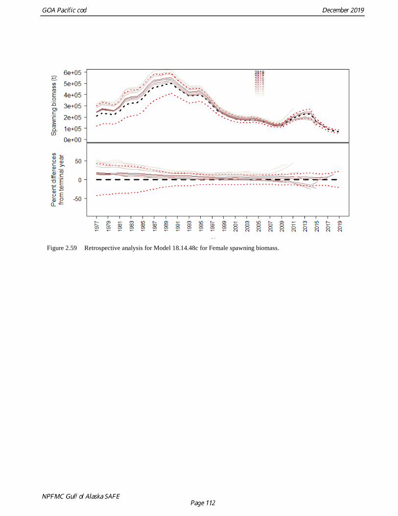
Figure 2.59 Retrospective analysis for Model 18.14.48c for Female spawning biomass.

Figure 2.60 Total biomass estimates from reviewed models and NMFS bottom trawl survey biomass estimates

with 95% confidence bounds.

Figure 2.61 Selectivity curves for Model 19.14.48c Trawl fishery (FshTrawl), longline fishery (FshLL), pot

fishery (FshPot), NMFS bottom trawl survey (Srv), and AFSC Longline survey (LLSrv) length

composition data.

Figure 2.62 Overall Model 19.14.48c fits to Trawl fishery (FshTrawl), longline fishery (FshLL), pot fishery

(FshPot), NMFS bottom trawl survey (Srv), and AFSC Longline survey (LLSrv) length composition

data.

Figure 2.63 Trawl fishery length composition and Model 19.14.48c fit (top and left) and mean length (cm; right bottom).

Figure 2.64 Trawl fishery length composition Pearson residuals (max = 8.01).

Figure 2.65 Longline fishery length composition and Model 19.14.48c fit (top and left) and mean length (cm; right bottom).

Figure 2.66 Longline fishery length composition and Model 19.14.48c fit (top and left) and Pearson residuals (max = 5.25).

Figure 2.67 Pot fishery length composition and Model 19.14.48c fit (top), mean length (bottom left), and Pearson residuals (max=4.61; bottom right).

Figure 2.68 NMFS bottom trawl survey length composition and Model 19.14.48c fit (top), Pearson residuals (left

bottom; max = 9.66), and mean length (cm; right bottom).

Figure 2.69 AFSC Longline survey length composition and Model 19.14.48c fit (top), Pearson residuals (left bottom; max=5.19), and mean length (cm; right

bottom).

Figure 2.70 NMFS bottom trawl survey (Srv) age composition and Model 19.14.48c fit (left). Note the age data

fits are not included in the objective function.

Figure 2.71 Model 19.14.48c length at age, weight at age, weight at length, and fraction mature at length, weight,

and age.

Figure 2.72 NMFS bottom trawl survey (Srv) conditional length-at-age data and Model 19.14.48c fit.

Figure 2.73 Trawl fishery conditional length-at-age data and Model 19.14.48c fit.

Figure 2.74 Longline fishery conditional length-at-age data and Model 19.14.48c fit.

Figure 2.75 Pot fishery conditional length-at-age data and Model 19.14.48c fit.

Figure 2.76 Model 19.14.48c predicted spawning output (femal spawning biomass; t) with 95% asymtotic error

intervals (top) and total biomass (t).

Spaw

nin

g B

iom

ass

(t)

Figure 2.77 Model 19.14.48c predictions of middle of the year number at age (top) with mean age (red line) and

numer at length (bottom)with mean length (red line).

Figure 2.78 Model 19.14.48c age-0 recruitment (1000’s) with 95% asymtotic error intervals.

Figure 2.79 Model 19.14.48c log recruitment deviations with 95% asymtotic error intervals.

Figure 2.80 Model 19.14.48c age 3-8 true fishing mortality (top) and continuos fishing mortality by trawl

(FshTrawl), longline (FshLL) and pot (FshPot) fisheries (bottom).

Figure 2.81 For Model 19.14.48c ratio of historical F/Fmsy versus female spawning biomass relative to Bmsy for

GOA pacific cod, 1977-2021. Note that the proxies for Fmsy and Bmsy are F35% and B35%,

respectively. The Fs presented are the sum of the full Fs across fleets. Dashed line is at B20%, Steller

sea lion closure rule for GOA Pacific cod.

Figure 2.82 Model 19.14.48c MCMC trace (top left), density (top right), autocorrelation function plot (bottom

left), and Geweke diagnostic plot (bottom right) for the objective function.

Figure 2.83 Model 19.14.48c MCMC posterior distribitions of beginning of the year female spawning biomass 1977-2023. Dotted line is the projected SSB20%,

the red dashed line is the projected SSB17.5%.

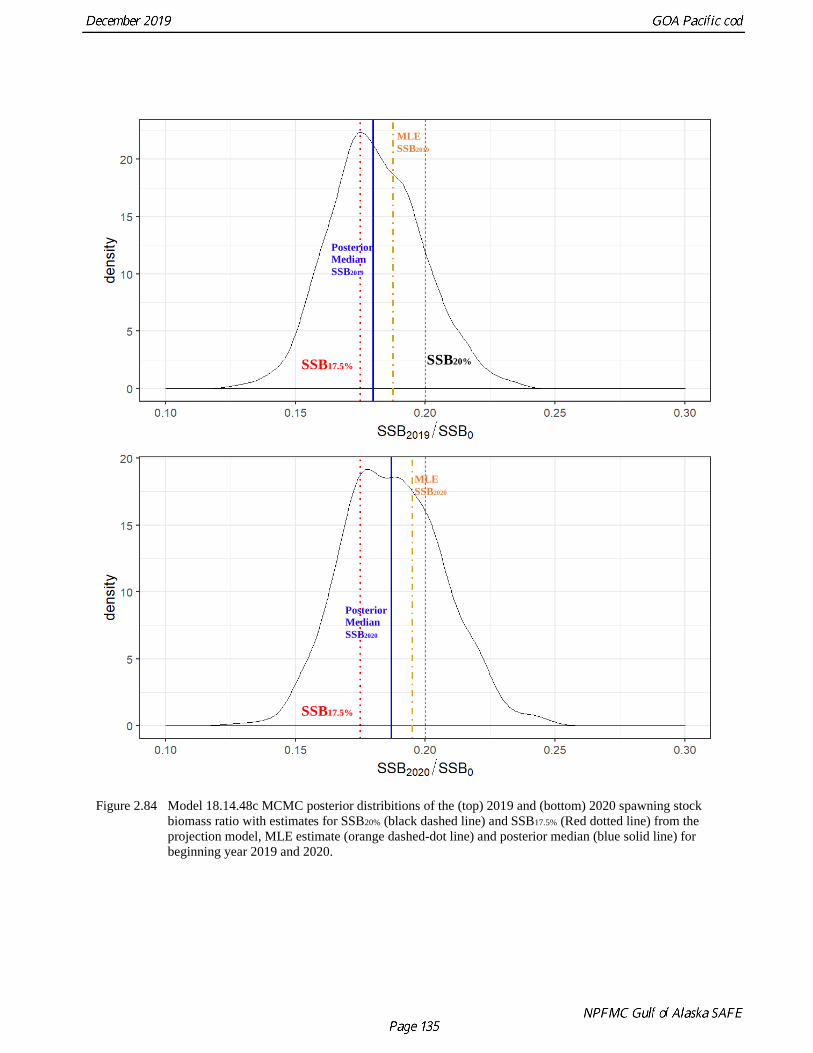
Figure 2.84 Model 18.14.48c MCMC posterior distribitions of the (top) 2019 and (bottom) 2020 spawning stock

biomass ratio with estimates for SSB20% (black dashed line) and SSB17.5% (Red dotted line) from the

projection model, MLE estimate (orange dashed-dot line) and posterior median (blue solid line) for

beginning year 2019 and 2020.

SSB17.5% SSB20%

MLE

SSB2019

Posterior

Median

SSB2019

Posterior

Median

SSB2020

MLE

SSB2020

SSB17.5%

Figure 2.85 Model 19.14.48c Age-0 recruits with and without the 2014-2016 fitting block on natural mortality

showing differences in estimated recruitment for 1977-2019.

Figure 2.86 Model 19.14.48c projections of female spawning biomass (top ), catch (bottom left), and female spawning biomass from scenarios 6 and 7 for status

determination (bottom right).

Figure 2.87 Cumulative f(T) function index based on 36 month moving window of thermal experience.

Figure 2.88 Pacific cod bioenergetic model (Holsman and Aydin, 2015; Holsman et al. in prep) estimates of foraging demand based on fish weight and CSFR age-specific depth-preference corrected water temperatures (Barbeaux, unpublished data).

Figure 2.89 Pacific cod bioenergetic model (Holsman and Aydin, 2015; Holsman et al. in prep) estimates of metabolic demand based on fish weight, survey bottom temperature, annual indices of GOA prey energy density and ration (g/g/d; based on groundfish surveys), and an intermediate P. cod energy density of 3.62 kJ/g reported in Vollenweider et al. (2011).

Figure 2.90 Pacific cod bioenergetic model (Holsman and Aydin, 2015; Holsman et al. in prep) estimates of growth potential based on fish weight, survey bottom temperature, annual indices of GOA prey energy density and ration (g/g/d; based on groundfish surveys), and an intermediate P. cod energy density of 3.62 kJ/g reported in Vollenweider et al. 2011.

Figure 2.91 Specific weight (g prey/ g pred/ d) of prey in the diets of GOA Pacific cod, averaged across all survey diet samples and fish sizes. Diet data from NOAA REEM Food Habits database.

Figure 2.92 Average prey energy density based on mean energy density of prey items and diet composition from GOA Pacific cod stomach samples