Embed Size (px)
Citation preview

1
ASSESSMENTOFFIBRECONTENTAND3DPROFILEINCYLINDRICALSFRCSPECIMENS
Sergio H. P. CAVALARO1*, Rubén LÓPEZ-CARREÑO1, Josep María TORRENTS2, Antonio AGUADO1, Pablo JUAN-GARCÍA2
1 Departamento de Ingeniería de la Construcción, ETSECCPB, Universidad Politécnica de Cataluña, BarcelonaTech, Calle Jordi Girona 1‐3, 08034, Barcelona, España
2 Departamento de Ingeniería Electrónica, EEL, Universidad Politécnica de Cataluña, BarcelonaTech, Calle Jordi Girona 1‐3, 08034, Barcelona, España
* Corresponding author: Despacho 106, Edificio B1, Campus Nord, Departamento de Ingeniería de la Construcción, ETSECCPB, Universidad Politécnica de Cataluña, BarcelonaTech, Calle Jordi Girona 1‐3, 08034, Barcelona, España, email [email protected], Phone (+34) 934054247, Fax (+34) 934054135
Abstract
The inductive method proposed by Torrents et al. [1] and improved by Cavalaro et al. [2] is used
to assess the fibre content and distribution in steel fibre reinforced concrete, providing valuable
information for the design and the quality control. Despite several advantages, the method presents
limitations. On one hand, it was conceived for the test of cubic specimens, which complicates its
application in existing structures due to the difficulty to extract cubic cores. On the other hand, only a
partial characterization of the fibre orientation is obtained given that the determination is restricted to
the three axes of the specimen. With these measurements, it is not possible to derive the fibre
orientation in other directions different from the ones used to test the sample. The objective of this
paper is to propose an assessment of the fibre content and distribution in any direction using the
inductive method and cylindrical specimens. For that, first a modification of the method is proposed.
Then, new equations are deducted to generalize the test to samples with different shapes and to assess
the anisotropy level as well as the directions with the maximum and the minimum fibre contribution.
Next, an extensive experimental program and FEM numerical simulations are performed to validate and
to determine the accuracy of the formulation developed. The results show that the application of these
equations and the execution of only one additional measurement per specimen are enough to
determine the fibre profile in all in‐plane directions with a high accuracy.
Keywords: SFRC; inductive method; fibre content; orientation profile; quality control

2
1. INTRODUCTION
The increasing use of steel fibre reinforced concrete (SFRC) [1‐4] has generated the
need for tests that provide information about the material. Besides the traditional tests to
assess mechanical properties [5‐7], different techniques are required to evaluate the fibre
content and orientation. Both parameters are closely related with the quality and the
performance of SFRC [3], being of interest for the design of structures and for the systematic
quality control.
Several tests were developed with that purpose. An example is the inductive method
proposed by Torrents et al. [1] and improved by Cavalaro et al. [2]. As shown in Figure 1.a, the
equipment used in this test is composed by a LCR impedance analyser and a coil that receives
an electric current and generates a magnetic field. When a SFRC cubic sample is placed inside
the coil, a modification of the magnetic permeability of the medium is observed [12, 13]. This
modification leads to a change in the inductance [14] measured with the LCR impedance
analyser. The method takes advantage of the fact that steel fibres are several orders of
magnitude more magnetic than plain concrete [15]. This means that the test is highly sensitive
to the inclusion of even small amounts of steel fibres, whereas the concrete practically do not
affect the measurements regardless of its strength class or composition.
Figure 1. Inductive method by Torrents et al. [1] (a) and proposed modification (b)
The inductance change produced by the SFRC cubic specimen should be measured
once in each main direction since the contribution of the fibres is proportional to the angle
with the magnetic field inside the coil. Previous studies by Cavalaro et al. [2] proved that the
summed inductance in the three axes is linearly related to the fibre content. The same authors
also propose equations to estimate the orientation number based on the results obtained. This
capability, together with the small cost of the equipment and the small time required for the
characterization of each specimen, makes the inductive method an interesting alternative for
the systematic quality control of SFRC [16‐18].
Nevertheless, the method also presents limitations. For once, it was conceived and
validated for the test of cubic SFRC specimens, which present symmetry in the three axes. In
fact, the equations to predict the fibre content and orientation may not apply to specimens
Copper spirals
LCR impedance analysera)
Copper spirals
b)

3
with other shapes that do exhibit such symmetry. This complicates the use of the method in
existing structures (for instance segmental linings [19], pipes [20] or slabs [21]) due to the
difficulty to obtain cubic extracted cores. In this context, the possibility of performing the test
in cylindrical specimens would represent an improvement.
Furthermore, only a partial characterization of the fibre orientation is obtained with
the method given that the determination is restricted to the three axes of the cubic specimen.
Based on these results it is not possible to derive the orientation in different directions. In
other words, the results provide no clear view on how the fibre distribution varies for
directions different from the actually measured. If, for instance, the crack in the real structure
should not coincide with these directions, it would not be possible to derive the orientation
number and the fibre contribution perpendicular to the crack. This hinders the application of
the test in elements such as slabs or shells in which the position of the failure plane is not well
defined. It is also impossible to determine the degree of anisotropy of the sample or the
directions with the highest and smallest contribution of the fibres.
The consideration of all these aspects related with the fibre distribution in real
structures is one of the keystones of the most recent philosophy applied to the design of SFRC
elements [23, 24], which account for the favourable or unfavourable orientations. In this
context, the achievement of a more complete characterization of both moulded and extracted
specimens is an essential step.
Taking that into account, the objective of this paper is to propose and validate the
assessment of the fibre content and distribution in any direction using the inductive method
and cylindrical specimens. For that, first a modification of the method is proposed. Then, new
equations are deducted to generalize the test for samples with different shapes and to assess
the fibre distribution. Next, an extensive experimental program and FEM numerical
simulations are performed to validate and to determine the accuracy of the formulations
proposed. The results obtained show that the application of these equations and the execution
of only one additional measurement per specimen are enough to obtain the fibre distribution
profile in any in‐plane direction with a high accuracy. Now, parameters such as the minimum
and maximum fibre orientation number, as well as the direction in which these values occur,
may be easily obtained with the inductive method. This expands the potential of the
technique, providing a reliable and simple tool to support the quality control and to supply the
information required for a more refined design.
2. MODIFICATION OF THE METHOD
As in any method based in the inductance change, the accuracy of the measurement is
highly dependent on the homogeneity of the magnetic field generated. For instance, imagine a
field produced by a coil with a non‐homogeneous flux distribution, as shown Figure 2.a. If the
flux at one point (φ1) has the double of the magnitude than at another point (φ2), a fibre
placed in φ1 will produce an inductance change twice as big as that placed in φ2. Therefore, the

4
presence of non‐homogeneities would cause the same inclusion to produce different response
depending on the position inside the coil, thus compromising the reliability of the results.
Figure 2. Fibres inside a non‐homogeneous magnetic flux (a) and detail of magnetic field across
cubic (b) and cylindrical (c) specimens
Two important inferences may be derived from this analogy. On one hand it becomes
evident that to increase the accuracy of the method it is necessary to apply a magnetic field as
uniform as possible. On the other hand, since a perfectly homogeny field may not be achieved
in reality, the interaction between the magnetic field and the specimen will always depend on
its position inside the coil.
The equipment proposed by Torrents et al. [1] is composed by a discontinuous square
coil manufactured with a copper cable of 0.2 mm of diameter and a length of 1600 mm,
resulting in a total of 2354 turns. The dimensions of the prismatic plastic element around
which the coil is placed are 15 x 17 x 17 cm (see Figure 1.a). It is known that the square is not
the optimal cross section in terms of the homogeneity of the magnetic field generated inside
the coil. In fact, the presence of corners contributes to variations in the field. Another
associated problem arises if the test should be performed in specimens that do not show
symmetry in the three axes, like in cylindrical cores. In this case, slight changes in the angle of
the specimen relatively to the sides of the coil could induce additional scatter in the
measurements. Both problems may be mitigated if a circular shaped coil would be used
instead, leading to a more homogeny magnetic field and, ultimately, to less variability and
more accurate results.
A different design of coil was proposed according with this idea in order to obtain a
method suitable to cylindrical specimens. As shown in Figure 1.b, the new coil consisted of two
spirals separated 13 cm apart and connected in a parallel discontinuous configuration. Each of
them had a circular cross section with 25cm of interior diameter and was made of a copper
cable of 0.3 mm of diameter with a total of 1200 turns.
a)
b)
c)
5
In theory, the modification of the coil should not affect the equations proposed by
Cavalaro et al. [2] to predict the fibre content and orientation number for cubic specimens.
However, the deduction of more general equations that could be applied to the test of any
shape of sample and to estimate the fibre distribution in any direction is still required.
3. ANALYTICAL DEDUCTIONS
3.1. Fibre content
In this study, equations were deducted to assess the fibre amount for a SFRC specimen
with an unknown form and a volume V. To simplify the deduction, at first it is assumed that
fibres are uniformly dispersed in the concrete mass. Regardless of its shape, the specimen
could be discretised in the differential volumes dV with the same fibre content (Cf in weight by
unities of volume), as depicted in Figure 3.
Figure 3. Discretization of a specimen
The inductance change (dLi) produced by each differential volume when measuring in
an axis i may be calculated according with Eq. 1, based on the study by Cavalaro et al [2]. This
equation depends of the magnetic nature of the fibre (k’), the electric current (I) that goes
through the coil, the magnetic flux density (B) generated in this point and the angel αi formed
between the magnetic field and the fibre in the differential element. The equation is also
related with the shape factor that is constant for each type of fibre and may be obtained by
the ratio between the inductance of a single fibre perpendicular and parallel to the magnetic
field.
∙1
∙Eq.1
Integrating Eq. 1 in the whole volume gives Eq. 2 for the global inductance change
measured Li in the direction i. Notice that the parameter BV,i represents the integral of the

6
magnetic field over the volume of the sample. Such parameter does not depend on the fibre
used, being constant if the specimen is always placed in the same position and the coil is the
same.
,
∙∙
,
∙∙ , Eq.2
The sum of the inductance changes produced after measuring in three orthogonal axes
(x, y and z indicated in Figure 5) yields Eq. 3. It is easy to demonstrate that in cubic specimens,
the values of BV,x , BV,y and BV,z are equal due to the symmetry of the sample. Consequently, Eq.
3 may be reduced to Eq. 4. The latter could be further simplified since the angles αx, αy and αz
are complementary, meaning that x+y+z should equal the constant 1+2∙. Notice that all parameters in Eq. 4 are constant except for the fibre content and the summed inductance,
which should hold a linear relation with each other. Consequently, if the constant of
proportionality (’) is known in advance, the content of fibres could be estimated based on the
summed inductance obtained in the test. This agrees with the demonstrated by Cavalaro et al.
[2] and could be represented according with Eq. 5
, ,
∙∙ , ∙ , ∙ , Eq.3
,
, ,
∙,
∙, 1 2 ∙ Eq.4
′ ,
, ,
Eq.5
However, if a specimen without symmetry was tested, the values of BV,x , BV,y and BV,z
would not be the same. As a result, the simplifications used to obtain Eq. 4 and 5 would not
apply, meaning that the relation between the summed inductance and the fibre content
should not be linear. Consequently, it would not be possible to assess the fibre content
through the inductive method. To eliminate this problem and make the method applicable to
any shape of specimen, a mathematical artifice was used. Instead of calculating the summed
inductance in the three axes, the sum of the ratio between the measurement in each axis and
the corresponding constant BV,i should be used according with Eq. 6.
,, ,
∙ ∙1 2 ∙ Eq.6

7
Notice that the latter will reduce every time to x+y+z, which is constant and equal
to 1+2∙. In other words, the summed equivalent inductance (Le) should always be linearly
related with the fibre content. This suggests that the content of fibre could be estimated with
Le through Eq. 7 regardless of the shape of the specimen, being the formulation proposed by
Cavalaro et al. [2] and Torrents et al. [1] only a special case of it. In fact, Eq. 7 becomes Eq. 5 if
cubic specimens are considered.
,, ,
Eq.7
Comparing Eq. 6 and 7, it is possible to deduct the proportionality constant (see Eq. 8). It is usual to determine with one or two specimens by dividing the fibre content weighted
after crushing the specimen and the corresponding value of equivalent inductance (Le)
measured. This division gives the slope of the straight line that passes through the origin of the
coordinate system and relates the measurements of the inductive method and the fibre
content. Alternatively, this parameter may be assessed directly by using a known content of
fibres that is subjected to the inductive method in the three directions. Notice that according
with the new formulation proposed, should be the same for any shape of specimen and
concrete type.
1 2 ∙Eq.8
3.2. Orientation number and contribution of fibres
For the deduction of the equations that determine the fibre distribution consider the
same example from section 3.1. To simplify the initial deduction assume that all fibres are
arranged with the same direction. The orientation number (ηi) is given by the average of the
cosine of the angle formed between the fibres and a line parallel to at an axis i [25‐27]. The
average of the cosine ‐ equivalent to the average orientation number in the direction i ‐ may
be obtained by isolating the cosi in Eq.2. This gives Eq. 9, which may be combined with Eq. 7
and 8 to derive Eq. 10 for the assessment of the orientation number of a general specimen
with all fibres arranges in the same direction. It is important to remark that Eq. 10 reduces to
the proposed by Cavalaro et al. [2] if cubic specimens are considered.
11
∙ ∙∙ ,
Eq.9
∙ 1 2 ∙ ∙ , ∙∙ , ∙ 1
Eq.10

8
Eq. 10 is representative of a situation in which all fibres are aligned in the same
direction. In this context, the average of the cosine of the angle with the axis i equals the
square root of the average square cosine. Consequently, the orientation number may be easily
estimated through the results from the inductive method. Nevertheless, if the fibres are
dispersed with certain randomness, an overestimation could be obtained with Eq. 10 since the
average cosine of the angle with the axis i diverges from square root of the average square
cosine obtained with the inductive method. This mathematical incongruence was previously
explained by Cavalaro et al [2] who deducted that the average overestimation () per axis may
range from 0.07 and 0.10 depending on the specimen shape.
In order to compensate for this overestimation, the correction parameter must be
introduced in Eq. 10. Another parameter () should be included to account for the non‐homogeneity of the magnetic field that is not considered in the mathematical deductions. As a
result of both modifications, Eq. 11 is obtained for the prediction of the orientation number in
a general specimen with dispersed fibres. By definition, the fibre contribution (Ci) is still
calculated through Eq. 12.
∙∙ 1 2 ∙ ∙ , ∙
∙ , ∙ 1 Eq.11
∑ , , Eq.12
3.3. Generalization for cylindrical specimens
The equations derived for the assessment of the content of fibres (Eq. 7) and the
orientation numbers (Eq. 11) are valid for any type of specimen. To apply them, it is only
necessary to assess the constants BV,i, and corresponding to the shape of specimen and the
coil used. These parameters are not easy to obtain analytically since the assessment of the
magnetic field at any point requires solving a complex set of equations. A more direct
approach considered in this study consists of the application of an electromagnetic finite
element. The mesh used is composed by cubic brick elements with a side of 1 mm. The
magnetic flux density (B) and the magnetic field (H) follow Eq. 13 and Eq. 14, with J being the
electric current density. These are the classic equations from electromagnetism theory that are
valid for static magnetic fields, in which the wavelength produced by the current is much
bigger than the dimensions of specimens or of the coil.
0 Eq.13

9
Eq.14
Once the magnetic field is calculated it may be integrated over the volume occupied by
the specimen to obtain BV,i. The estimation of and requires the consideration in the finite element of the concrete and the dispersed fibre inside the coil. For that, the algorithm to
simulate the fibre distribution and the analogy for the inductance change proposed by
Cavalaro et al. [2] are taken into account. It is important to remark that this model has been
validated with experimental results.
Each SFRC specimen is simulated with the magnetic field acting in the three main
directions, thus reproducing the procedure conducted during the test. After performing
several simulations, the parameters and are estimated. Table 1 summarizes the
parameters for the assessment of the fibre content and orientation in any cylindrical and cubic
specimens. Notice that these parameters remain constant regardless of the concrete mix, fibre
content and type.
Table 1. Constant parameters for cylindrical and cubic specimens
Shape Size (mm) Parameter
BV,x BV,y BV,z
Cylindrical 100x100 536 536 538 0.085 1.03
150x150 1789 1789 1809 0.085 1.03
Cubic 100x100x100 695 695 695 0.100 1.03
150x150x150 2342 2342 2342 0.100 1.03
3.4. Orientation profile for cylindrical specimens
The use of cylindrical specimens not only is feasible through the general equations
proposed here, but also opens up the possibility of overcoming one of the main disadvantage
of the inductive method in its current configuration. As mentioned before, the method is not
capable of providing the fibre orientation in axes different from the ones used to measure the
inductance. Therefore, limited information is obtained when the crack does not coincide with
these directions and it is not possible to assess the anisotropy of the material in terms of the
maximum and minimum orientation number and their corresponding directions.
In any SFRC cylindrical specimen, the fibre distribution may be understood as the
superposition of two samples: one isotropic (Figure 4.a) and one with certain anisotropy
(Figure 4.b). If the inductance measurements are taken by spinning both samples at several
angles (), different behaviours would be observed. As shown in the graph from Figure 4.a, the
isotropic sample would show a constant inductance (Liso) since an evenly distributed number of
fibres is present in all directions. On the contrary, as depicted in the graph from Figure 4.b, the
inductance of the anisotropic sample should present maximum and minimums values that
coincide with the directions with more and less fibre contribution, respectively. Notice that the

10
minimum value could never be equal to 0 since the fibre produce an inductance change even if
placed perpendicular to the magnetic field. In this context, the final inductance measured in
the real specimen should be the result of the sum of the curves obtained for the isotropic and
anisotropic specimens (see Figure 4.c).
Figure 4. Detail and inductance profile of isotropic (a), anisotropic (b) and resultant (c)
specimens
Results by Laranjeira [25] and Grunewald [27] suggest that the variation of the angle
formed by the fibre and a certain axis may be represented through a Gauss or a Gumble
distribution. This indicates that the curve obtained for the anisotropic sample tend to have a
continuous shape with a clear maximum and minimum values. Consequently, it would be
possible to use the equations proposed in this study to predict the variation of the orientation
number depending without the need of performing several additional measurements.
Making an analogy with the equations deducted in section 3.2, the inductive change
(L) at a certain angle could be estimated mathematically through Eq. 15 that reflects the
superposition of two parts. The first of them represents the isotropic sample that should yield
a constant inductance equal to Liso. The second part represents the variation of the anisotropic
sample that may be approximated by means of Eq. 2, considering a maximum inductance Lani
observed at the angle with maximum fibre contribution (max).

11
1 ∙ Eq.15
Notice that the only unknowns that should be determined to obtain the change in
inductance are Liso, Lani and max, which will be constant for each specimen. To obtain them, a
system of three equations must be solved. Therefore, three measurements of inductance in
the XY plane are required. Given that by default one measurement is already taken in the X
axis and another in the Y axis, it is possible to derive the complete profile of fibre distribution
with only one additional assessment in the XY plane. In order to improve the reliability of the
predictions, the additional measurement should be performed in the intermediate direction
that forms and 45 angle with X and Y, as depicted in Figure 5. It is important to remark that
this represents a change in the usual procedure applied up to date in the inductive method.
Instead of performing 3 measurements, 4 are required to achieve a complete characterization
of the specimen. By convention, it is assumed that the axes X and Y coincide with the angle of
0° and 90°, respectively.
Figure 5. Measurement axes to obtain the orientation profile
Solving the system of equations for the measurements in X (L0), Y (L90) and the
intermediate direction (L45) gives Eq. 16, 17 and 18 for the estimation of Lani, Liso and max.
Using Eq. 15, it is also possible to obtain the angle that will give the minimum inductance (min)
through Eq. 19. Notice that the formulation for the assessment of max has an initial sign that
might be positive or negative since two angles satisfy the arc cosine. A simple mathematical
proof should be performed with equation Eq. 15 to determine the correct angle. The results
obtained for the angles of 0°, 45° and 90° are compared with the measured experimentally
that served as input parameters for the analysis. The correct angle should provide identical
results for all measurements.
√21 ° ° ° ° 2 ∙ °
Eq.16

12
° ° ∙ 12
Eq.17
12∙ ° °
∙ 1Eq.18
90° Eq.19
The orientation number may now be estimated at any axis with an angle by introducing in Eq. 12 the inductances L and L+90 estimated with Eq.15 for the same angle and
for + 90. This is represented mathematically through Eq. 20.
1.03 ∙∙ 1 ° ∙ ,
,∙
° ∙ ,
,∙ 1
0.085 Eq.20
3.5 Isotropy of the fibre distribution
The maximum (Lmax) and the minimum (Lmin) inductance may be assessed by
introducing Eq. 16 and 17 in Eq. 15. The results are presented in Eq. 21 and 22.
Eq.21
∙ Eq.22
As indicated by Eq. 19, the maximum and the minimum value of inductance should be
separated by 90. Consequently, the maximum (ηmax) and the minimum (ηmin) orientation
numbers corresponding to the same angles may be estimated by using Lmax and Lmin in Eq. 20.
This leads to Eq. 23 and 24, respectively.
1.03 ∙∙ 1 ∙ ,
,∙
∙ ,
,∙ 1
0.085 Eq.23

13
1.03 ∙∙ 1 ∙ ,
,∙
∙ ,
,∙ 1
0.085 Eq.24
The possibility of estimating the complete orientation profile with one additional
inductance measurement allows the proposal of a parameter related with the level of isotropy
of SFRC. This parameter, called isotropy factor (Ω), is defined in Eq. 25 as the ratio between
ηmin and ηmax. It may assume values ranging from nearly 0 to 1. If the fibre distribution is
perfectly isotropic, ηmax and ηmin acquire the same value and Ω equals 1. Otherwise, if all the
fibres are aligned in the same direction, the value of ηmax is orders of magnitude bigger than
ηmin and the Ω tends to 0.
Eq.25
4. EXPERIMENTAL VALIDATION
In total, three experimental programs were conducted in order to confirm the accuracy
of the equations deducted in the present study. One of them was dedicated to validate the
formulations proposed for assessing the fibre content in section 3.1. Another was performed
to contrast the equations for assessing the orientation number and the contribution of the
fibres from sections 3.2 and 3.3. A third experimental program was conducted to confirm the
predictions for the orientation profile based on the formulation proposed in sections 3.4
and 3.5.
4.1. Fibre content
4.1.1. Materials and methods
In order to evaluate the fibre content, cubic specimens with 150 mm of edge and
cylindrical specimens with 150 mm of diameter and height were tested with the inductive
method and then crushed to assess the weight of fibre. The specimens were cast with 6
concrete mixes, using 2 types of concretes (conventional and self‐compacting) as well as 3
nominal fibre contents (30, 45 and 60 kg/m3).
The steel fibres used in the SFRC were BASF Masterfiber 502 with a circular cross‐
section of 1 mm diameter, 50 mm of length and hooked ends. These fibres are made of low
carbon steel with approximately 3000 unities per kg. A 250 litres vertical mixer was used to
produce batches of 120 l, which was enough to cast all samples of the same mix. Table 1
presents the composition of the concrete mixes tested and their fresh state properties
14
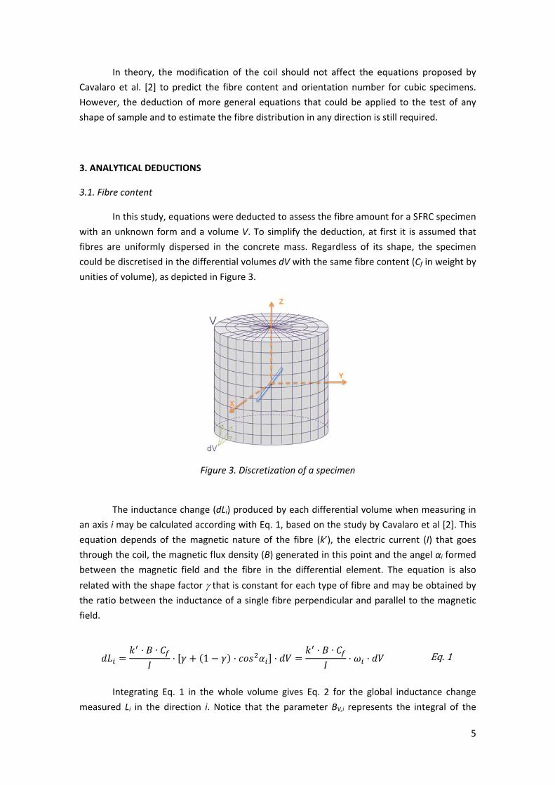
measured. For each mix and geometry, 4 specimens were produced in accordance with EN
12390‐2.
Table 2. Concrete mixes tested
Components Characteristics Content (kg/m³)
Conventional Self‐compacting
Gravel (12/20 mm) Granite 810 200
Gravel (5/12 mm) Granite 404 500
Sand (0/5 mm) Granite 817 1200
Cement CEM I 52,5 R 312 380
Water ‐ 156 165
Superplasticizer Glenium TC 1425 2.19 4.56
Hidratation activator X SEED 6.24 7.6
Fibres Steel fibres 30 45 60 30 45 60
Reference CC30 CC45 CC60 SC30 SC45 SC60
Slump (mm) according UNE 83503 3 5 3 ‐ ‐ ‐
Flow extent (mm) according EN 206 ‐ ‐ ‐ 650 650 670
In the first step of the testing procedure, the three main axes of the specimen were
marked. In the case of cylindrical samples, the Z axis was the revolution axis parallel to the
casting direction, whereas the axes X and Y were randomly selected. For the cubic, the Z axis
was parallel to the casting direction while the axes X and Y were parallel to the sides of the
moulds. The second step consisted of measuring the inductance for the three directions. For
that, the modified coil shown in Figure 1.b was used. The input of the electrical current and the
inductance measurements were performed with the equipment AGILENT LCR 4263B. The
electrical current was set as alternating with a frequency of 1 kHz and a voltage of 1 V.
Finally, the fibre content was estimated according with the EN 14721. A hydraulic press
was used to crack the specimens that were then crushed in a grinding machine. Afterwards,
the fibres were manually separated with the help of a magnet and weighted. Considering the
laborious and long time required, this procedure was performed only in 20 specimens: 10
cylindrical and 10 cubic. In each group, 5 specimens were of conventional concrete and 5 were
of self‐compacting concrete.
In this study, the accuracy of the formulation developed is evaluated in terms of the
trueness and the precision. The trueness is given by the mean difference between the real
values measured in the experimental program and the estimated with the equations
developed in previous sections. It marks how close the average predictions are from the
reality, being small values indicative of high accuracy. The precision is obtained as the the
standard deviation of the differences between estimated and real values. It provides
information on how individual values might vary around the average. Once more, small values
indicate higher precision.
4.1.2. Results and analysis
Figure 6 shows the fibre content (Cf) assessed after crushing and the equivalent
inductance (Le) calculated from the inductances as proposed in section 3.1 for cubic and

15
cylindrical specimens. It is evident that a linear relation exists between Le and Cf. Notice that
despite considering specimens of different shapes, the results fit to the same linear regression
with a R2 of 0.99. The linear regression starts approximately at the origin of the coordinate
system and assumes a slope approximately equal to 5909.4.
Figure 6. Relation between equivalent Inductance and fibre content
The average trueness calculated as de difference between the fibre content measured
and the predicted with the equivalent inductance is 0.38 kg/m³. The value obtained
considering only the cylindrical or the cubic specimens are 0.46 kg/m³ and ‐0.33 kg/m³,
respectively. Such small errors may be considered negligible taking into account the usual fibre
content in SFRC and the wide range measured in the experimental program (from 20 kg/m³ to
almost 100 kg/m³), thus confirming the high accuracy of the method. These results validate the
formulation proposed in section 3.1 to estimate the fibre content. It confirms that the
consideration of the summed equivalent inductance (Le) should be the reference parameter to
assess the fibre content since the same calibration curve applies regardless of the shape of
specimen characterized. Likewise, good predictions are achieved for both conventional and
self‐compacting concrete.
4.2. Orientation of fibres
4.2.1. Materials and methods
With the intent of evaluating the equations for the orientation number and the
contribution of fibres, a cylindrical specimen with a known fibre orientation was made by
hand. For that, 13 layers of non‐magnetic cardboard sheets were cut in a circular shape and
glued together in order to form a specimen with 150 mm of diameter and 150 mm of height,
as shown in Figure 7.
0
20
40
60
80
100
0 5 10 15
Fiber content Cf(kg/m
3)
Equivalent inductance Le (x10‐3)
b) Cf = 5909.4LeR² = 0.988

16
Figure 7. Cardboard specimen with aligned fibres
In total, 243 g of fibres of the same type used in the first experimental program were
placed between adjacent sheets. All fibres were distributed uniformly along the height with
the same alignment, being orthogonal to the theoretical axis of the specimen (Z axis). The
specimen was then tested with the inductive method. Measurements were taken at the Z axis
and in the XY plane for the angles of 0°, 10°, 20°, 30°, 40°, 50°, 60°, 70°, 80° and 90° between
the alignment of the fibres and the direction of the magnetic field.
4.2.2. Results and analysis
Figure 8.a shows the curves for the real orientation number and the estimated with Eq.
10 by using the results of the inductive method. Both curves practically coincide. The trueness
and the precision from the proposal indicate an error of prediction that might be considered
negligible, again confirming the accuracy of the equations developed here.
Figure 8. Variation of the orientation number (a) and the fibre contribution (b) depending on
the angle of measurement for the cardboard specimen
0,0
0,2
0,4
0,6
0,8
1,0
0 30 60 90
i()
Angle αi (°)
a)
0,0
0,2
0,4
0,6
0,8
1,0
0 30 60 90
Ci()
Angle αi (°)
b)

17
Figure 8.b presents the real contribution of fibres and the estimated with the values of
inductance and Eq. 12. In the same way as the orientation number, the real and the calculated
curves practically overlap. Once more, the low values of trueness and precision suggest a
negligible error in the predictions. The high accuracy corroborates the efficacy of the equations
and confirms that the integrals of magnetic flux density were well calculated.
4.3. Orientation profile
4.3.1. Materials and methods
The 24 cylindrical specimens produced in the first experimental program were also
used to validate the equations proposed to obtain the orientation profile. The aim was to
evaluate if the predictions with Eq. 15 to 19 agrees with the values actually measured. For
that, the specimens were marked with 8 directions of measurement in the XY plane separated
22.5° from each other, as shown in Figure 9. The inductance was evaluated in each direction as
well as along the Z axis. To avoid favouring a better fit of the data, the directions used to
estimate the orientation profile were selected randomly prior to the test.
Figure 9. Axes of measurements in a cylindrical specimen
4.3.2. Results and analysis
Figure 10.a shows the orientation profile measured and estimated for two of the
specimen characterized. The estimations were performed with Eq. 15 to 18 and the
inductances for the angles of 0°, 45° and 90°. All samples presented a similar trend regardless
of the fibre content or the concrete type. The results reveal that the complete inductance
profile is well reproduced by Eq. 15 to 18. As predicted, the profiles show the same period (180
degrees) but different amplitudes that is related with the level of anisotropy of the samples.

18
Figure 10. Inductance profile (a) and comparison between real and estimated values (b)
Figure 10.b presents the real inductance measured at different angles and the
estimated with Eq. 15 to 19 for all samples tested. It is evident that the equations proposed
are capable of predicting the experimental results with a high accuracy. In fact, the theoretical
estimation had a trueness of 0.04% and a precision of 1.01% in relation with the
measurements. Both results confirm that it is feasible to estimate the inductance and the
orientation profile with only one additional measurement in the XY plane.
Figure 11 presents the comparison between the real values obtained in the
experimental program and the ones estimated with the simplified equations deducted
previously. This evaluation is performed for the maximum (Lmax) and the minimum (Lmin)
inductance calculated, as well as for the direction (θmax) with the maximum contribution and
the direction (θmin) with the minimum contribution. In the case of the experimental results, a
linear regression was used to assess these parameters, whereas in the analytical approach the
equations proposed here were used with the measurements at 0°, 45° and 90°.
Figure 11. Comparison between real and estimated values for Lmax (a), Lmax (b), max (c) and for
min (d) based on the experimental results
0
2
4
6
8
10
0 45 90 135 180
L estim
ated(m
H)
Angle (°)
a)a)a)a)
0
2
4
6
8
10
0 2 4 6 8 10
L estim
ated(m
H)
L real (mH)
b)
0
3
6
9
12
0 3 6 9 12
L estim
ated(m
H)
L real (mH)
a)
‐90
‐45
0
45
90
‐90 ‐45 0 45 90
estim
ated(°)
real (°)
b)
19
The figures reveal that the basic parameters that determine the fibre distribution
profile are well predicted by the model developed. A small error is obtained in all cases.
Observe, for instance, the error of prediction of the direction with the maximum and the
minimum fibre contribution. In both cases, the real values are predicted with a trueness
smaller than 1°. Similar outcome is also verified for the maximum and the minimum
inductance, in which even better predictions are achieved.
5. NUMERICAL VALIDATION
The experimental programs demonstrate the effectiveness of the formulation
proposed here. Although specimens with perfectly aligned fibres or with 3 nominal fibre
contents and 2 concrete types were tested, it is important to consider that in practice other
levels of anisotropy may occur. Moreover, although only cast samples were characterized, in
practice it should be also feasible to obtain the fibre distribution for extracted cores. In this
context, it is advisable to evaluate the equations proposed for cast and extracted samples with
a wider range of anisotropy levels. However, this is not easy to perform experimentally
provided the difficulty to control de fibre distribution and the limitation in terms of resources
to assess such a wide range of concrete types.
Therefore, instead of performing this verification based on additional experimental
results, a numerical approach similar to the already conducted by Cavalaro et al. [2] was
performed. The viability of this approach was confirmed by the authors for 15 cm edge cubic
specimens and for a square coil. In the present study, a similar finite element model (FEM) was
first developed and validated. Then it was used to evaluate the accuracy of the formulation
proposed for the assessment of the orientation number, the contribution and the orientation
profile.
5.1. Description and validation of the FEM
The FEM developed contained two modules. In the first of them, several probabilistic
laws are responsible for defining the distribution and the orientation of each fibre within a
concrete specimen that could be either cast in a mould or extracted from an existing structure.
Aspects such as the geometry of the sample, the wall‐effect of the formwork in cast specimens
[28‐30] and the cut of fibres in extracted specimens were taken into account. Once the fibres
are distributed inside the specimen, the second module calculates the inductance change
produced in the circular coil when the inductive test is performed. The magnetic field
generated by the coil is implemented simulating the same conditions as in the experimental
program. Finally, with the inductance change and the distribution of fibres, the model is able
to compare the real fibre distribution and the predicted with the inductance measurements.
For more details on the FEM, check Cavalaro et al [2].

20
To validate the FEM applied in the numerical study, the cardboard specimen from the
experimental program described in section 4.2 was simulated and the inductance changes
were assessed for several angles. Figure 12 presents the inductances estimated with the FEM
and measured in the laboratory for equivalent angles. The values of trueness and precision of
the inductance predicted with the FEM are 0.0735 and 0.1632, respectively. Such values
indicate that the FEM is capable of reproducing the inductance change in the coil due to the
presence of fibres.
Figure 12. Comparison between the inductance measured in the laboratory and the results of
the FEM for a cylindrical coil
5.2. Parametric study
Once the FEM was validated simulations were performed considering a wide range of
levels of anisotropy in the fibre distribution. The different distributions were achieved by
modifying the values of the director vectors ,
and ,
that govern the probability of
finding fibres in each of the main axes. For instance, if all axes shared the same value of these
parameters, an approximately isotropic distribution would be obtained in zones not influence
by the wall‐effect. Consequently, almost the same number of fibres would be observed in all
directions. On the contrary, if one axis presented a smaller ,
or ,
, fibres would
have a lower probability of appearing alongside directions that approach this axis. In the
simulations ,
varied from ‐0.5 to ‐1.0 and ,
ranged from 0.5 to 1.0.
Each level of anisotropy was simulated for of 0.000, 0.025 and 0.050 that account for the inclusion of fibres with different aspect ratios. A shape factor of 0 represents a theoretical
situation in which the diameter of the fibre is negligible in comparison with its length. On the
other hand, a shape factor of 0.05 is representative of the fibre used in the experimental
program.
The combination of parameters led to 63 cases, all of them consisting of the simulation
of the inductive test of cylindrical cast specimens with fibre content of 60 kg/m³. For each
case, 20 models were analysed in order to derive a representative sample. This approach is
necessary since the probabilistic laws behind the fibre distribution in the FEM produce a
slightly different specimen every time. Therefore, a minimum number of models are required
0
2
4
6
8
10
12
14
0 2 4 6 8 10 12 14
Inductan
ce with FEM
(mH)
Inductance measured (mH)

21
to perceive a clear trend. Specimens were simulated and the inductance change was assessed
in the Z axis and at every 15° in the XY plane.
These simulations were repeated for extracted cores. Contrarily to the observed in cast
specimens that have a fibre orientation induced by the lateral surface of the moulds, the
extracted cores are not affected by this wall‐effect. Instead it presents several fibres that are
cut during the extraction process. To simulate these conditions, no lateral restriction to the
position of the fibre was considered. Furthermore, the stretches of fibre that extend beyond
the lateral extraction boundary were eliminated since in reality they would be cut.
5.3. Results and analysis
5.3.1. Orientation number
Figure 13.a shows the relation between the real orientation number of the specimens
modelled with the FEM and the calculated with Eq. 11 using the inductance change for the
same specimens. The results from the simulations performed with cast and extracted samples
are included in the figure. Notice that the orientation numbers obtained cover the usual range
found in practice, reaching even extreme values that unlikely would be observed. Despite that,
the estimated orientation numbers agree with the real ones in the whole range considered. In
fact, the trueness and the precision of the estimations suggest an average error far below
0.5%.
Figure 13. Comparison between real and estimated orientation number (a) and fibre
contribution (b) for cast and extracted samples
Figure 13.b shows analogous results for the fibre contribution using Eq. 12. Such
results confirm the accuracy of Eq. 11 and 12 for the assessment of fibre contribution and
orientation number based on the inductive method applied for cylindrical specimens. This
remains true regardless of the type of sample, the aspect ratio of the fibres or the degree of
anisotropy.
0,2
0,3
0,4
0,5
0,6
0,7
0,8
0,2 0,3 0,4 0,5 0,6 0,7 0,8
ηestim
ated()
η real ()
a)
0,1
0,2
0,3
0,4
0,5
0,6
0,1 0,2 0,3 0,4 0,5 0,6
C estim
ated()
C real ()
b)

22
5.3.2. Orientation profile
The inductance obtained with the FEM at the angles of 0°, 45° and 90° in the XY plane
were used to derive the complete inductance profile according with Eq. 15 to 19 for any
direction. This profile is then compared with the real ones. This comparison for all models
considered in the parametric study is presented in Figures 14.a.
Figure 14. Comparison between real and estimated inductance profile (a) and orientation
profile (b)
It is observed that the profile calculated with the FEM agrees with the obtained by
using the simplified formulation developed here. The same outcome remains true when
orientation profiles estimated with Eq. 20 are compared with the actual fibre distribution from
the specimen, as shown in Figure 14.b. This confirms that the estimation of the inductance and
the orientation profile is possible with only one additional measurement for a wide range of
levels of anisotropy and different fibre types. In fact, the new formulation proposed and the
test of cylindrical specimens allows detecting the orientation number in axes different from
the ones used for the measurement, thus providing a much clearer picture of the fibre
distribution in SFRC elements.
Verifications were also performed to evaluate the accuracy of the predictions of Lmax,
Lmin, θmax, θmin, ηmax, ηmin, and according with Eq. 21, 22, 18, 19, 23, 24 and 25, respectively.
The estimations were compared with the values calculated for the same specimens with the
FEM. Figure 15 presents the results obtained.
10
15
20
25
30
35
40
10 15 20 25 30 35 40
L estim
ated(m
H)
L real (mH)
a)
0,3
0,4
0,5
0,6
0,7
0,3 0,4 0,5 0,6 0,7ηestim
ated()
η real ()
b)

23
Figure 15. Comparison between real and estimated values for Lmax and Lmin (a), max and min (b),
ηmax and ηmix (c) and Ω (d) based on the numerical analysis
In all cases, the formulation proposed remains accurate even if extreme values are
considered. This is observed especially for the maximum and minimum inductance and
orientation number, which show average errors below 0.5%. Good results are also obtained
for θmax and θmin, with a trueness that indicates an average error of prediction below 1.5°. In
the comparison shown in Figure 15.d between the real and the estimated isotropy factor () a
noteworthy fit is obtained regardless of the level of isotropy because of the accurate
prediction of ηmax and ηmin.
6. CONCLUSIONS
In this work, an increase in the capability of predicting the fibre content and
distribution with the inductive method applied to specimens with any shape was achieved.
After analytical deductions, several equations were proposed and then validated with an
extensive experimental and numerical study. The following are the main conclusions derived
from this work.
10
15
20
25
30
35
40
10 15 20 25 30 35 40
L estim
ated(m
H)
L real (mH)
a)
‐90
‐45
0
45
90
‐90 ‐45 0 45 90
estim
ated(°)
real (°)
b)
0,2
0,4
0,6
0,8
0,2 0,4 0,6 0,8
ηestim
ated()
η real ()
c)
0,4
0,6
0,8
1,0
0,4 0,6 0,8 1,0
estim
ated()
real ()
d)

24
A modified coil was designed. This coil is more compatible with the test of specimens
that do not present symmetry in the three axes (such as the cylindrical ones) since it
tends to reduce potential variability in the results.
The analytical deductions indicate that the formulation currently used to predict the
fibre content in cubic specimens could lead to errors if applied to specimens without
symmetry in the three axes. A new approach valid regardless of the shape of the
specimen and based on the equivalent inductance (Le) was proposed in the present
study. The experimental program performed with cubic and cylindrical specimens
confirm that with this approach the same calibration curve applies to both specimens
with an average error of only 380 g/m³. The good accuracy is verified for both
conventional and self‐compacting concrete.
The numerical validation shows that the formulation proposed to determine the
orientation number of the fibres (Eq. 11) and their contribution in one direction (Eq.
12) based on the results from the inductive method in cylindrical specimens is capable
of estimating the real values with an average trueness below 0.5%. Negligible errors of
prediction are obtained in cast or extracted specimens for a wide range of orientation
numbers.
The equations deducted expand the application of the inductive method, allowing the
determination of the orientation number in any direction (Eq. 15 and 20). The validity
of these equations was confirmed experimentally and in numerical simulations. A high
accuracy of the predictions is obtained in both cases, with trueness and precision
values that are below 0.43% and 1.69%, respectively.
The inductive method may now be used to assess in a simplified way the maximum
and minimum orientation numbers (Eq. 23 and 24), as well as the directions in which
these values occur (Eq. 18 and 19). Such assessment may serve to determine potential
planes of weakness of real scale element. Moreover, a new parameter was proposed
to quantify the degree of anisotropy of SFRC (Eq. 25) based on the maximum and the
minimum orientation number. The experimental and the numerical validations
indicate that all these parameter may be obtained only by applying the equations
proposed here and by performing 4 measurements per sample instead of the 3
currently used. This minute additional effort leads to a much more complete
assessment of the characteristics of SFRC, providing the information required for the
quality control and the design according with the most recent guidelines.
ACKNOWLEDGEMENTS
The authors thank PROMSA for the support during the experimental program and the
Ministerio de Economía y Competitividad for the financial support provided within the project
FIBHAC (IPT‐2011‐1613‐420000).
25
REFERENCES
[1] Torrents JM, Blanco A, Pujadas P, Aguado A, Juan‐García P, Sánchez‐Moragues MÁ
(2012) Inductive method for assessing the amount and orientation of steel fibers in
concrete. Mater Struct 45(10):1577‐1592
[2] Cavalaro SHP, López R, Torrents JM, Aguado A (2014) Improved assessment of fibre
content and orientation with inductive method in SFRC. Mater Struct, 1‐15
[3] Serna P, Arango S, Ribeiro T, Núñez AM, Garcia‐Taengua E (2009) Structural cast‐in‐
place SFRC: technology, control criteria and recent applications in Spain. Mater Struct
42(9):1233‐1246
[4] di Prisco M, Plizzari G, Vandewalle L (2009) Fibre reinforced concrete: new design
perspectives. Mater Struct 42(9):1261‐1281
[5] CEN. EN 14651:2005 (2005) Test method for metallic fibrered concrete ‐ Measuring the
flexural tensile strength (limit of proportionality (LOP), residual), European Committee
for Standardization, Brussels
[6] RILEM TC 162‐TDF (2003) Test and design methods for steel fibre reinforced concrete‐
σ‐ε design method: final recommendation. Mater Struct 36(262):560–567
[7] IBN. NBN B 15‐238 (1992) Essais des bétons renforcés de fibres ‐ Essai de flexion sur
éprouvettes prismatiques, Institut Belge de Normalisation Brussels (In French)
[8] Mobasher B, Stang H, Shah SP (1990) Microcracking in fiber reinforced concrete. Cem
Concr Res 20(5):665‐676
[9] Pujadas P, Blanco A, Cavalaro SHP, de la Fuente A, Aguado A (2014) Multidirectional
double punch test to assess the post‐cracking behaviour and fibre orientation of FRC.
Constr Build Mater 58:214‐224
[10] Ferrara L, Meda A (2006) Relationships between fibre distribution, workability and the
mechanical properties of SFRC applied to precast roof elements. Mater Struct
39(4):411‐420
[11] Blanco A (2013) Characterization and modelling of SFRC elements. PhD Thesis,
Universitat Politècnica de Catalunya
[12] Polder D, Van Santeen JH (1946) The effective permeability of mixtures of solids.
Physica 12(5):257‐271.
[13] Sihvola AH, Lindell IV (1992) Effective permeability of mixtures. Progr Electromagn Res
6:153‐180

26
[14] Faifer M, Ferrara L, Ottoboni R, Toscani S (2013) Low Frequency Electrical and
Magnetic Methods for Non‐Destructive Analysis of Fiber Dispersion in Fiber Reinforced
Cementitious Composites: An Overview. Sensors 13(1):1300‐1318
[15] Ferrara L, Faifer M, Toscani S (2012) A magnetic method for non destructive
monitoring of fiber dispersion and orientation in steel fiber reinforced cementitious
composites—part 1: method calibration. Mater Struct 45(4):575‐589
[16] Maturana A, Sanchez R, Canales J, Orbe A, Ansola R, Veguería E (2010) Technical
economic analysis of steel fibre reinforced concrete flag slabs. A real building
application. XXXVII IAHSWorld Congress on Housing
[17] Orbe A, Cuadrado J, Losada R, Rojí E (2012) Framework for the design and analysis of
steel fiber reinforced self‐compacting concrete structures. Constr Build Mater 35:676‐
686
[18] Orbe A, Rojí E, Losada R, Cuadrado J (2014) Calibration patterns for predicting residual
strengths of steel fibre reinforced concrete (SFRC). Compos Part B‐Eng 58:408‐417
[19] de la Fuente A, Pujadas P, Blanco A, Aguado A (2011) Experiences in Barcelona with the
use of fibres in segmental linings. Tunn Undergr Space Technol 27(1):60–71
[20] de la Fuente A, Escariz RC, de Figueiredo AD, Molins C, Aguado A (2012). A new design
method for steel fibre reinforced concrete pipes. Constr Build Mater 30:547‐555
[21] Pujadas P, Blanco A, de la Fuente A, Aguado A (2013) Cracking behavior of FRC slabs
with traditional reinforcement. Mater Struct 45(10):1577–1592
[22] Pujadas P, Blanco A, Cavalaro SHP, Aguado A (2014) Plastic fibres as the only
reinforcement for flat suspended slabs: experimental investigation and numerical
simulation. Constr Build Mater 57:92–104
[23] Laranjeira de Oliveira F (2010) Design‐oriented constitutive model for steel fiber
reinforced concrete. PhD Thesis, Universitat Politècnica de Catalunya
[24] CEB‐FIB (2010) Model Code. Comité Euro‐International du Beton‐Federation International de la Precontraint, Paris
[25] Laranjeira F, Grünewald S, Walraven J, Blom C, Molins C, Aguado A (2011)
Characterization of the orientation profile of steel fiber reinforced concrete. Mater
Struct 44(6):1093–1111
[26] Laranjeira F, Aguado A, Molins C, Grünewald S, Walraven J, Cavalaro S (2012) Framework to predict the orientation of fibers in FRC: a novel philosophy. Cem Concr Res 42(6):752–768
[27] Grünewald S (2004) Performance‐based design of selfcompacting fibre reinforced
concrete. PhD Thesis, Delft University of Technology

27
[28] Kameswara Rao CVS (1979) Effectiveness of random fibres in composites. Cem Concr
Res 9(6):685–693 [29] Soroushian P, Lee CD (1990) Distribution and orientation of fibers in steel fiber
reinforced concrete. ACI Mater J 87(5):433–439 [30] Martinie L, Roussel N (2011) Simple tools for fiber orientation prediction in industrial
practice. Cem Concr Res 41(10):993–1000