Assessment 30 min 30 min 50 minutes 30 min 50 …...intersection using what we call a D/D/1 queuing model. We are assuming deterministic arrivals, deterministic service pattern, and

Traffic Signal Systems – Operations and Design – Facilitation Guide

39 (2012.12.19)

CHAPTER 2: MODELING WHAT WE’VE OBSERVED: QUEUING SYSTEMS This chapter includes information that you will need to prepare for, conduct, and assess each of the seven activities included in Chapter 2 of the student activity book. Figure 1 shows the various files that are available to support your works as you use these activities, including mini-lecture slides, solution files, and student resource files.

Figure 1. Support files

Figure 2 shows the kind of work required for each activity, how the activities might be grouped, and the approximate amount of class time required to complete the activity. The figure also identifies whether there is homework involved, a mini-lecture could be presented, student discussion could take place, and group work to do.

Figure 2. Activity work

Chapter 2Modeling What We’ve Observed

A#08Reading

A#09Assessment

A#10Discovery

A#11Field

A#12In Practice

Mini-lecture slides Solution filesStudent resource

files

Chapter 2Modeling What We’ve Observed

A#08Reading

A#09Assessment

A#10Discovery

A#11Field

A#12In Practice

30 min 30 min 50 minutes 30 min

Mini-lecture

Homework

Student discussion

Group work

50 minutes

Chapter 2: Modeling What We’ve Observed: Queuing Systems

40 (2012.11.19)


41 (2012.12.19)

Using Activity #8: Modeling Traffic Flow at Signalized Intersections (Reading) Overview This activity requires the student to read the “Information” section, define the terms and variables listed in the Glossary, and answer the “Critical Thinking Questions.” This activity is generally assigned as homework. Students will learn how queuing system theory can be used to represent, both graphically and mathematically, traffic flow at signalized intersections. In chapter 2, we begin to look at modeling or representing traffic flow at a signalized intersection in a way that will help us estimate or measure how an intersection is or might perform under a given set of input conditions. The type of model that we will use in this chapter is called a queuing model. Options for Use The reading, defining the terms in the glossary, and answering the critical thinking questions are usually done as homework. After the students complete this work, the instructor has several options for assessing and clarifying student understanding of the reading during class:

Discussion and synthesis of the answers to the quiz, the glossary definitions, and answers to the critical thinking questions. (30 minutes)

Preparing for the Activity

Decide which of the options you want to do during class.

Prepare for the class by reviewing Activity #8, including the “Information”, the Glossary definitions, and Critical Thinking Questions and answers.

Review the script and slides that are provided. Doing the Activity (Script) [Slides: slides08.pptx] 1. Provide your perspective on the reading that they have just completed and how it fits into

the course. Discuss how this reading fits into chapter 2, an introduction to the application of queuing models to traffic signal control systems.

2. As a way of encouraging students to complete a reading assignment in preparation for class, it is often useful to have a quiz or discussion to “test” their knowledge and to allow them to validate their understanding.

3. The following script can be used along with the slides for this activity. The script and slides can be modified based on your needs and what you decide to emphasize for this activity.


42 (2012.11.19)

Slide Script

In this chapter, we are focusing on ways or models to represent traffic flow at signalized intersections, and what these models can tell us about intersection operations and performance. We will also learn or see that some initial assumptions that we make will have to be relaxed or changed when we starting looking at conditions that we find in the real world. So, we are studying traffic flow on one approach of a signalized intersection using what we call a D/D/1 queuing model. We are assuming deterministic arrivals, deterministic service pattern, and one service channel. Alternative wording: In chapter 2, we begin to look at modeling or representing traffic flow at a signalized intersection in a way that will help us measure or estimate how an intersection is performing or might perform under a given set of conditions. The type of model that we will use in this chapter is called a queuing model. A queue is simply a line of objects or people waiting to be served (or: waiting to pass through a point to continue their trip)

Here is a video of traffic arriving and departing from a signalized intersection. It is about 50 seconds in length. Watch the vehicles first queue up during red. Then at the beginning of green, the queue that has built up begins to clear, at the saturation flow rate. Once the queue has cleared, vehicles arrive and leave with no delay.

You read A#8 which focused on some of the basics of how queuing theory can be applied to traffic flow at signalized intersections. Ask:

What is a queuing system? [Queue comes from the Latin word meaning “tail”. A queuing system is a system in which people or things wait for some kind of service. “Queuing theory, originally developed to model the nation’s telephone system, is based on a system that includes users who desire to be served in some way, a server, and a process for serving these users.”]

Which elements of a traffic control system are included in a queuing model? [We need to consider the arrival process and the service process. The arrival process is described by a flow rate, usually vehicles per hour, as well as the manner in which vehicles

A#8 2

A#8 3

Some questions – queuing systems

• What is a queuing system?• Which elements of a traffic control system are included in the queuing system?

• Which elements of traffic flow can you represent in a time space diagram

• What is a queue accumulation polygon and what information does it show about intersection operation and performance?


43 (2012.12.19)

Slide Script

arrive: uniform, random, some other distribution]. The service process depends on the signal status and sometimes on the opposing flow (when there are permitted left turns). The server is the place where the first vehicle in line is waiting to be served, at a traffic signal or stop sign. The queue is the second and following positions.

We represent the process in four ways:

Time space diagram (which is part of the traffic control process diagram that we saw earlier.

Flow profile diagram

Cumulative vehicle arrival and departure diagram

Queue accumulation polygon Ask a student to (or you can) draw on the board:

Flow profile diagram

Cumulative vehicle diagram

Queue Accumulation polygon Reiterate the basic assumption (or ask them):

Arrival pattern? Uniform.

Demand less than capacity; queue clears before end of green.

[People at checkout line] Ask: What do you see here? Here is a common queuing system that you have seen and used many times. A checkout counter. You put your groceries on the counter, the clerk serves you (rings up the purchase), and you leave.

Here is an aerial view of the intersection of 6th/Deakin, showing the aerial view of a queuing system, with labels for the various parts of the system.

Here is another view of the same intersection (6th/Deakin) showing the server (the first vehicle position at the stop line) and the queue (all other vehicles waiting in line).

A#8 4

A#8 5

A#8 6


44 (2012.11.19)

Slide Script

Here is the first way of representing traffic arriving and leaving from a signalized intersection using a time space diagram. Ask: what can we learn from this diagram? [Note each of the numbered parts of the slide.]

1. The shock wave of the forming queue. 2. The shock wave of the departing queue. 3. The delay experienced by each vehicle (or more specifically,

the time stopped). 4. The headway between each vehicle. 5. The speed of each vehicle. 6. The gap between the rear of one vehicle and the front of

the following vehicle (which we will later note as unoccupancy time).

We can also note here that the headways between each vehicle are equal; we call this uniform flow. This will be important as we review the charts to follow.

Draw on board:

Flow profile diagram [what can we learn from this diagram]

Cumulative vehicle diagram [show key points on sketch]

Queue accumulation polygon [show key points]

Draw on board: Derive equations for queue clearance (service) time (gq):

( )

Derive equations for uniform delay model. Total delay:

(

)

Average delay:

A#8 7

Display status

Dis

tan

ce

Time

12

3

4

5

6


45 (2012.12.19)

Slide Script

( )

( )

(

)

Solve example problem [see notes for example problem]

Queue clearance time

Uniform delay equation

Queue length at any time

Delay for any vehicle

[Flow profile diagram] Here is another representation of traffic flow, the arrival rate and the service rate. This shows uniform flow, or a constant arrival rate during the signal cycle.

[Cumulative vehicle diagram] Here is another representation, the cumulative number of vehicles that have arrived and departed from the intersection. Why are there two departure rates? Answer: one during the queue discharge and the other after the queue has cleared.

[Cumulative vehicle diagram showing delay for one vehicle] What is represented by the horizontal line in the figure? [Ask them] Answer: this time between the arrival and departure of a vehicle; we can represent this time as delay experienced by the vehicle.

[Cumulative vehicle diagram showing delay for four vehicles and shaded area showing total delay] If we add all of the horizontal lines representing each vehicle that arrives and departs, this gives us the total delay experienced by all vehicles. This is simply the area of the triangle.

A#8 8

A#8 9

A#8 10

A#8 11


46 (2012.11.19)

Slide Script

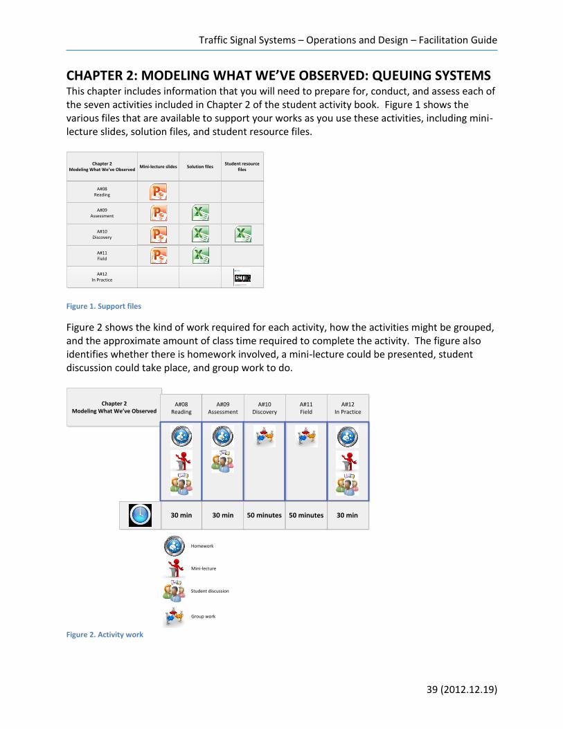
[Cumulative vehicle diagram showing queue at any point in time, t] What is the vertical line? [Ask them] Answer: the number of vehicles in queue at any given point in time.

[Queue accumulation polygon] What is the queue accumulation polygon? [Ask them] Answer: this is just the queue at any point in time, and is the vertical distance over time from the previous figure.

[Queue accumulation polygon, shaded area showing total delay] The area of the QAP is the same area that we observed before in the cumulative vehicle diagram; it is the total delay experienced by all vehicles arriving during one cycle.

Solutions The solutions presented here include:

Glossary definitions

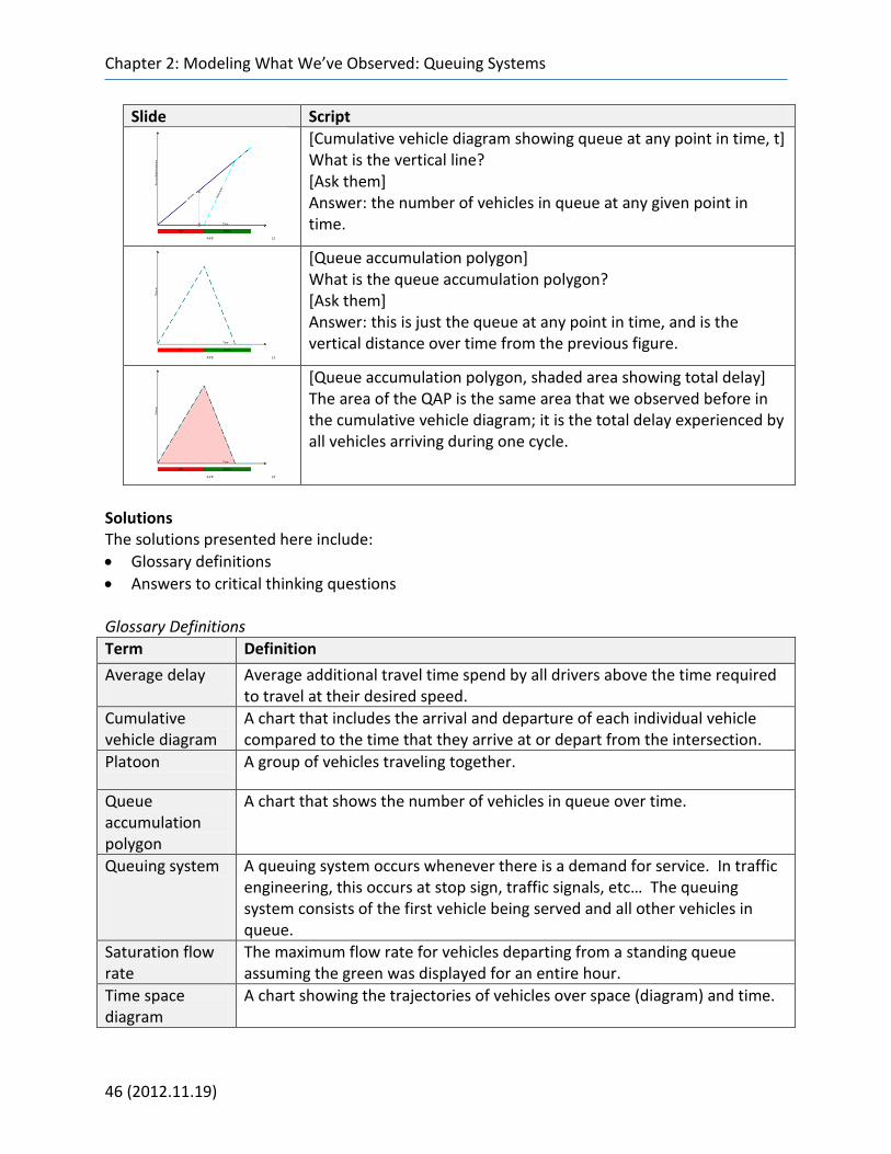
Answers to critical thinking questions Glossary Definitions

Term Definition

Average delay Average additional travel time spend by all drivers above the time required to travel at their desired speed.

Cumulative vehicle diagram

A chart that includes the arrival and departure of each individual vehicle compared to the time that they arrive at or depart from the intersection.

Platoon A group of vehicles traveling together.

Queue accumulation polygon

A chart that shows the number of vehicles in queue over time.

Queuing system A queuing system occurs whenever there is a demand for service. In traffic engineering, this occurs at stop sign, traffic signals, etc… The queuing system consists of the first vehicle being served and all other vehicles in queue.

Saturation flow rate

The maximum flow rate for vehicles departing from a standing queue assuming the green was displayed for an entire hour.

Time space diagram

A chart showing the trajectories of vehicles over space (diagram) and time.

A#8 12

A#8 13

A#8 14


47 (2012.12.19)

v Volume, vehicles per hour

t Time, seconds

r Duration of red time, seconds

g Duration of green time, seconds

gq Queue service time or queue clearance time, the time that is required for a standing queue to clear during the green display, seconds

s Saturation flow rate, vehicles per hour of green

dt Total delay experienced by all vehicles traveling through an intersection during one cycle

td Time that the ith vehicle departs from the intersection

ta Time that the ith vehicle arrives at the intersection

da Average delay experienced by all vehicles traveling through the intersection

c (lowercase) Capacity, vehicles per hour

C (uppercase) Cycle length, seconds

X Degree of saturation or ratio of volume to capacity.

Answers to Critical Thinking Questions: 1. What is a queuing system?

A queuing system occurs whenever there is a demand for service. In traffic engineering, this occurs at stop signs and traffic signals. The queuing system consists of the first vehicle being served and all other vehicles in queue.

2. Which elements of a traffic control system are included in the queuing system?

User

Detector

Controller

Signal display 3. Which elements of traffic flow can you represent in a time space diagram?

Vehicle trajectory (speed, acceleration, position)

Queue length (number of vehicles and distance)

Flow rate 4. What is a queue accumulation polygon and what information does it show about

intersection operation and performance?

The queue accumulation polygon graphs the queue length on the y-axis and time on the x-axis

Total delay

Max queue length


48 (2012.11.19)

5. How realistic is the uniform delay equation or model?

On a cycle by cycle basis, the uniform delay equation is not accurate because of variation in arrivals. However, to approximate traffic flow over a longer duration of time, the uniform delay equation will be a good representation because the delay variations observed on a cycle by cycle basis will average out to be the same as the uniform delay value.

6. What performance measures can the cumulative vehicle diagram show?

Total delay

Average delay

Max queue length 7. What are the elements common to a flow profile diagram, a cumulative vehicle diagram,

and a queue accumulation polygon?

Arrival rate

Departure rate

Service rate


49 (2012.12.19)

Using Activity #9: What Do You Know About Queuing Systems? (Assessment) Overview Activity #9 gives the students the chance to assess what they learned from the reading in Activity #8, particularly the graphical representation of traffic flow at a signalized intersection using queuing theory including flow profile diagrams, arrival departures diagram, and queue accumulation polygons. The reading introduces students to time space diagrams (trajectory diagrams), flow profile diagrams, cumulative vehicle diagrams, queue accumulation polygons, queuing theory and how to calculate uniform delay (both total delay and average delay), as well as queue length. The time space diagrams show vehicles responding to red and green indications. The trajectory diagrams also show forming and clearing shockwaves, saturation headway and arriving vehicular headways. The cumulative vehicle diagram and the queue accumulation polygon are presented and are used to facilitate a discussion about how to calculate uniform delay. Options for Use The activity can be done as homework or during class. Students should construct the various diagrams individually, so that they can test their knowledge and understanding of the reading from Activity #8.

Complete sketches of queuing diagrams. [individual]

Review sketches with partner and synthesis of answer to Critical Thinking Question. Preparing for the Activity

Decide which options you want to use during class and as preparation for class.

Review the reading in Activity #8.

Review the sketches required in Activity #9, as well as the solutions for the sketches. Doing the Activity (Script) [Slides: slides09.pptx] The following script can be used along with the slides for this activity. The script and slides can be modified based on your needs and what you decide to emphasize for the activity.

Slide Text

Provide your perspective on using models (with both advantages and limitations), especially the application of queuing theory to traffic flow at signalized intersections.

Ask them to consider what is included in the models: (which characteristics of traffic flow) and what assumptions are made (uniform arrivals, fixed time control)

Invite them to read the activity.

Ask them to answer the Critical Thinking Question and complete the sketches from Tasks 1 and 2.

Discuss results (see script and slides for solutions):

A#9 1


50 (2012.11.19)

Slide Text

o Students can do sketches at the board o Ask CTQ o Model assumptions, limitations

Task 1-1

A#9 2

Red Green

s

v arrival rate

Flo

w r

ate

Time

service rate

A#9 3

Task 1-2

Red Green

arrivals

Accu

mu

late

d v

eh

icle

s

Time

depa

rtur

es

A#9 4

Task 1-3

Red Green

Qu

eu

e

Time

Task 2- Case 1-1

A#9 5

Red Green

s

v arrival rate

Flo

w r

ate

Time

service rate

A#9 6

Task 2- Case 1-2

Red Green

arrivals

Accu

mu

late

d v

eh

icle

s

Time

depa

rtur

es

A#9 7

Task 2- Case 1-3

Red Green

Qu

eu

e

Time

A#9 8

Task 2- Case 2-1

Red Green

s

v arrival rate

Flo

w r

ate

Time

service rate


51 (2012.12.19)

Slide Text

Solutions

Excel file with example solutions. You can modify these examples as needed for studying additional cases. (solution09.xlsx)

Tasks 1 and 2 asks students to draw a sketch showing the flow profile of the arrival flow and departure flow at a signalized intersection for a period of one cycle for various conditions. Following are the three sketches for Task 1, which is the base condition discussed in the reading from Activity #8:

A#9 9

Task 2- Case 2-2

Red Green

arriva

ls

Accu

mu

late

d v

eh

icle

s

Time

depa

rtur

es

A#9 10

Task 2- Case 2-3

Red Green

Qu

eu

e

Time

A#9 11

Task 2- Case 3-1

A#9 12

Task 2- Case 3-2

Red Green

arrivals

Accu

mu

late

d v

eh

icle

s

Timedepartu

res

A#9 13

Task 2- Case 3-3

Red Green

Qu

eu

e

Time


52 (2012.11.19)


53 (2012.12.19)

In task 2, three cases are given and students are asked to sketch the three queuing diagrams for case. Case 1:

Red Green

s

v arrival rate

Flo

w r

ate

Time

service rate

Red Green

arrivals

Accu

mu

late

d v

eh

icle

sTime

depa

rtur

es

Red Green

Qu

eu

e

Time


54 (2012.11.19)

Case 2:

Red Green

s

v arrival rate

Flo

w r

ate

Time

service rate

Red Green

arriva

ls

Accu

mu

late

d v

eh

icle

s

Time

depa

rtur

es

Red Green

Qu

eu

e

Time


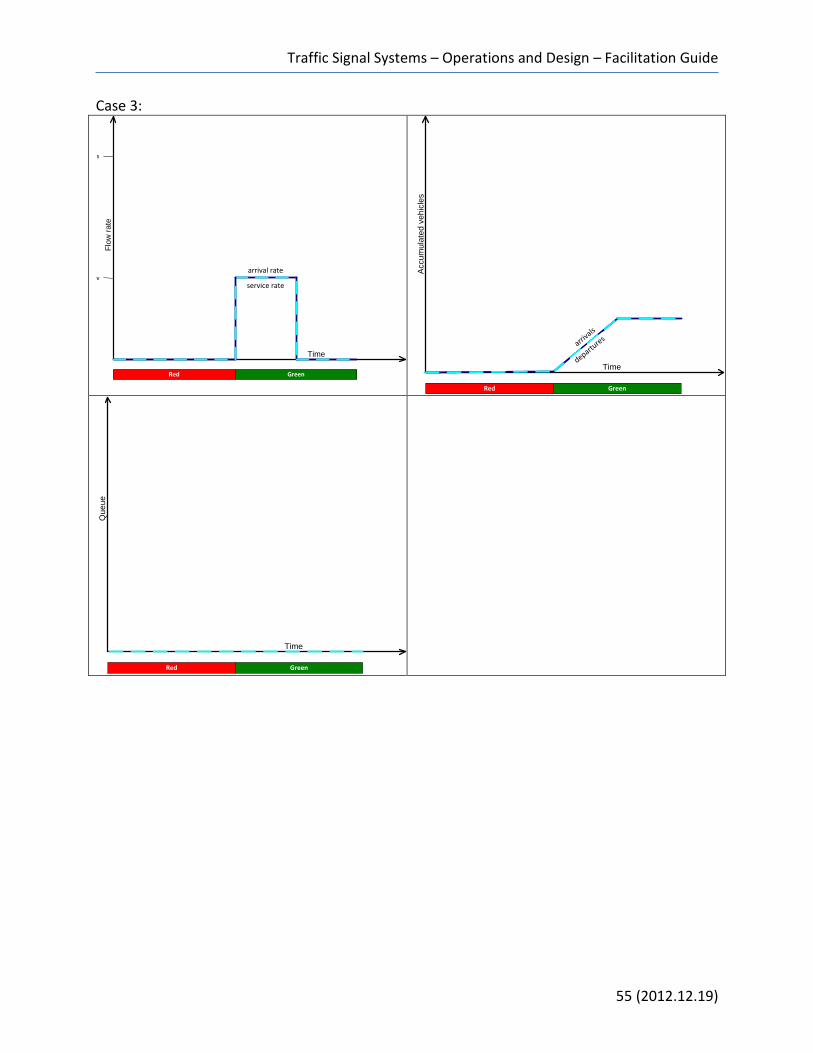
55 (2012.12.19)

Case 3:

Red Green

s

varrival rate

Flo

w r

ate

Time

service rate

Red Green

arrivals

Accu

mu

late

d v

eh

icle

s

Timedepartu

res

Red Green

Qu

eu

e

Time


56 (2012.11.19)


57 (2012.12.19)

Using Activity #10: Using High Resolution Field Data to Visualize Traffic Flow (Discovery) Overview The purpose of this activity is for students to see how the queuing models can represent real traffic flow conditions using data from the FHWA NGSIM project. Options for Use This activity can be done either in class or as homework. Preparing for the Activity

Determine whether you will conduct this activity during class or assign it as homework.

Review the activity description and tasks, and review the NGSIM data set that students will use for the project.

Doing the Activity (Script) [Slides: slides10.pptx] The following script can be used along with the slides for this activity. The script and slides can be modified based on your needs and what you decide to emphasize for the activity.

Slides Text

So let’s review for just a bit what we talked about yesterday and what you read and did in Activity #8 and Activity #9. We want to be able to represent traffic flow at a signalized intersection with queuing theory approach.

Now the specific queuing model that we use is called a D/D/1 model. Arrivals are deterministic (uniform, constant rate), service is deterministic (three time periods, each with a constant flow rate), and one service channel (one lane on approach).

We generally represent the queuing model in three ways, graphically (draw on board or show with slides): flow profile diagram, cumulative vehicle diagram, and queue accumulation diagram.

While this model provides a powerful and informative look at traffic flow at a signalized intersection, and is a good starting point, there are a number of realities that we must consider when we place our model in the real world. For example:

Arrival flow is generally not uniform during the cycle; sometimes there is a platoon that arrives at a given point during the cycle, or sometimes that platoon is random.

Sometimes the queue doesn’t clear before the end of green (D>C) and we have what a call a cycle failure (sometimes called a phase failure).

There is lost time at both the beginning and end of green that

1


58 (2012.11.19)

Slides Text

slightly “rounds” the arrival curve on the flow profile diagram.

Even the saturation flow rate during queue clearance is not uniform, with variations in the headways about the saturation headway.

To help us, we will look at a project funded through the FHWA whose purpose was to study how to improve traffic simulation models. This project was called NGSIM, or next generation simulation. Here is the web site.

Part of the project involved collecting very high resolution data of driver behavior at two freeway sites and two arterial sites. You “drove along” one of the sites, Lankershim Blvd, last week and this is the building on top of which the video data collection cameras were placed.

And here is a short excerpt showing the raw video first, and then how the data extraction worked, with the “numbering” of vehicles as the software recognized the vehicle and begin recording its trajectory along the arterial.

This brings us to Activity #10: read purpose, learning outcomes, review five tasks, look at spreadsheet file, read through tasks.

[draw on board] One other point. In our original queuing theory model, we assumed that all of the activity took place at a point: the queue stacked vertically above the server. Our real world system has another dimension. [show figure of real system showing entry point and exit point of the system]

Tell: So, the purpose of this activity (as well as the one to follow are to help you make the link between the neat world of modeling and the messiness of the real world. We will discuss both activities, one in which you will use a data set collected in the field and the other in which you collected data yourself. For both activities, we want to discuss three aspects:

The mechanics of the work: did you do the steps correctly.

The results or the data or charts that you generated.

What conclusions you made by looking at (studying) the data and charts, and what you learned about traffic flow and traffic signals in the process.

2

www.ngsim-community.org

3

4

5


59 (2012.12.19)

Slides Text

[solution]

[solution]

[solution]

[solution]

Solutions The solutions presented here include:

Excel spreadsheet file with data and charts [solution10.xlsx]

Answers to critical thinking questions Data file and solutions The data and charts produced by this activity are presented in the spreadsheet file, solution10.xlsx. Additional notes are provided below. Task 1: Using the field data, prepare a time-distance plot for the eight vehicles, placing distance on the y-axis and time on the x-axis. Note that the location of the stop bar for the subject intersection is at a distance of y = 346 feet. The stop bar location should be shown on the plot.

This is accomplished by creating a scatter plot of the data found in the “field data” tab of the a10.xlsx Excel file. Each vehicle should be plotted as a separate data series. The stop bar can be added by plotting a ninth data series, with x-values of zero and 200 and y values of 346 and 346. Two y values of 346 are necessary to create the horizontal stop bar. The resulting plot should look like the graph shown in Figure 1.

The "reaction" of each vehicle to passing through the subject intersection is shown. Vehicle 1 does stop near the stop bar, at Y = 346 as noted above. Vehicle 8, while not affected by

9

0

500

1000

1500

2000

0 50 100 150 200 250

Dis

tan

ce, f

eet

Time, sec

VehID = 1

VehID = 2

VehID = 3

VehID = 4

VehID = 5

VehID = 6

VehID = 7

VehID = 8

Stop bar

10

200

250

300

350

400

20 40 60 80 100 120

Dis

tan

ce, f

eet

Time, sec

VehID = 1

VehID = 2

VehID = 3

VehID = 4

VehID = 5

VehID = 6

VehID = 7

VehID = 8

Stop bar

11

1

2

3

4

5

6

7

8

0 20 40 60 80 100 120

Nu

mb

er

of

veh

icle

s

Time, sec

arrivals

departures

12

1

2

3

4

5

6

7

8

0 20 40 60 80 100 120

Nu

mb

er

of

veh

icle

s

Time, sec

arrivals

departures

61.4s

62.1s

58.5s

25.8s

2.9s

2.3s

1.1s1.4s


60 (2012.11.19)

the subject intersection, does stop at a downstream intersection. None of the other vehicles stop at this downstream intersection.

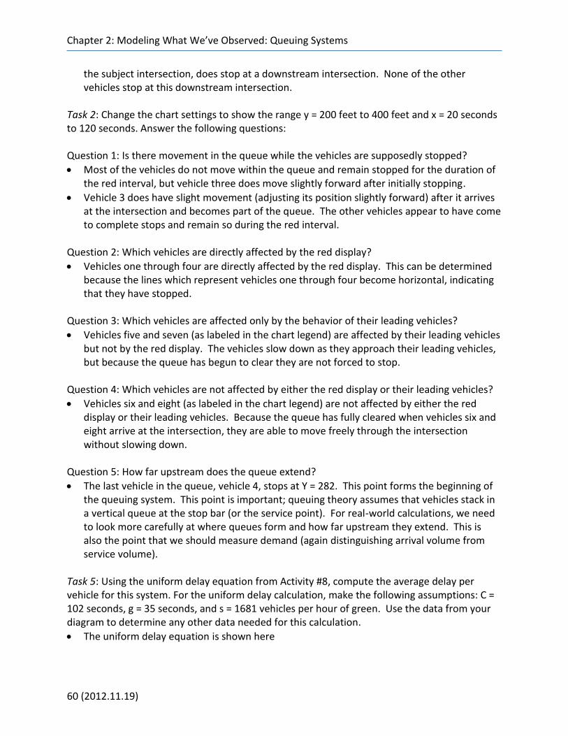
Task 2: Change the chart settings to show the range y = 200 feet to 400 feet and x = 20 seconds to 120 seconds. Answer the following questions: Question 1: Is there movement in the queue while the vehicles are supposedly stopped?

Most of the vehicles do not move within the queue and remain stopped for the duration of the red interval, but vehicle three does move slightly forward after initially stopping.

Vehicle 3 does have slight movement (adjusting its position slightly forward) after it arrives at the intersection and becomes part of the queue. The other vehicles appear to have come to complete stops and remain so during the red interval.

Question 2: Which vehicles are directly affected by the red display?

Vehicles one through four are directly affected by the red display. This can be determined because the lines which represent vehicles one through four become horizontal, indicating that they have stopped.

Question 3: Which vehicles are affected only by the behavior of their leading vehicles?

Vehicles five and seven (as labeled in the chart legend) are affected by their leading vehicles but not by the red display. The vehicles slow down as they approach their leading vehicles, but because the queue has begun to clear they are not forced to stop.

Question 4: Which vehicles are not affected by either the red display or their leading vehicles?

Vehicles six and eight (as labeled in the chart legend) are not affected by either the red display or their leading vehicles. Because the queue has fully cleared when vehicles six and eight arrive at the intersection, they are able to move freely through the intersection without slowing down.

Question 5: How far upstream does the queue extend?

The last vehicle in the queue, vehicle 4, stops at Y = 282. This point forms the beginning of the queuing system. This point is important; queuing theory assumes that vehicles stack in a vertical queue at the stop bar (or the service point). For real-world calculations, we need to look more carefully at where queues form and how far upstream they extend. This is also the point that we should measure demand (again distinguishing arrival volume from service volume).

Task 5: Using the uniform delay equation from Activity #8, compute the average delay per vehicle for this system. For the uniform delay calculation, make the following assumptions: C = 102 seconds, g = 35 seconds, and s = 1681 vehicles per hour of green. Use the data from your diagram to determine any other data needed for this calculation.

The uniform delay equation is shown here


61 (2012.12.19)

The only unknown value in the equation is v, which is the volume. This can be obtained by assuming that the number of vehicles shown in this example is consistent for every cycle, which in this case is 282 veh/hr.

Critical Thinking Questions Question 1: Consider the two estimates of delay from tasks 4 and 5. Why are they different? How would you refine your calculation method from task 4 to reduce this difference in the two delay estimates?

The two estimates of delay are different because the estimate made in Task 4 uses field data while the estimate made in Task 5 assumes uniform arrivals. Although these estimations are very close to each other, the estimate of Task 4 could become closer to that of Task 5 if the free flow time was reduced. If a free flow time of 1.0 seconds was used, the average delay would be only 0.6 seconds different from the uniform delay calculation.

The average delay is a more valid estimate of delay because it uses field data while the uniform delay does not. Uniform delay assumes that the vehicles arrive uniformly, but the data shows that only 7.6 seconds separates vehicles one and three, and that 10.5 seconds separate vehicles five and eight but vehicle three is separated from vehicle four by 35.9 seconds and vehicle four is separated from vehicle five by 24.3 seconds. The variance in times between vehicles demonstrates that the assumption of uniform arrivals is not completely valid. Even though the average delay (25.6 s) and the uniform delay (26.4 s) are similar, a large difference might occur if data was collected over a longer period of time.

Field measurement is always considered more valid. Often, the difference between the field measurement and a model estimate can be large. At first glance, these two values (25.7 vs 26.4) are much closer than we usually observe. However, we need to consider the basic assumption in this model: are the arrivals uniform or not? The answer? No.

[Other thoughts: The delay calculated in task 4 is based on the actual arrivals and departures. However, there is a non-zero travel time from the entry point into the system (Y=280) to the exit point (Y=346). We can estimate this travel time using the data for vehicles 7 and 8 that do not stop (note that vehicles 5 and 6 have some slow down time, so their times are not really free flow travel times).

Question 2: Compare the cumulative vehicle diagram that you prepared in Task 3 with the one that you sketched in Task 1 of Activity #9. Describe and explain any differences in these two diagrams.

The cumulative vehicle diagram created in Task 3 differs from those made in Tasks 3 through 5 of Activity 6 because those made in Activity 6 have perfectly straight lines. This is because uniform arrivals were assumed while the cumulative vehicle diagram created for Activity 7 uses field data and therefore each line has a different slope as it moves from one point to the next.


62 (2012.11.19)

Other notes to consider

One other chart that you can prepare shows the average arrival rate on the cumulative vehicle plot and the area that result. It shows that the real data can be very close to the theoretical average value.

Learn to make judgments about differences between two quantities and whether these differences are significant. There is a difference between what I would call "practical significance", which asks is there a difference that matters, and a "statistical significance", in which we make assumptions about the distributions of two groups and determine if the difference is caused by chance or not. More on this as we proceed during the semester.

What is right, model or data? How can data be wrong? (data collection errors, others). How precise or accurate do we need to be?

What assumptions to make (how to compute v, for example)?


63 (2012.12.19)

Using Activity #11: From Model to the Real World: Field Observations (Field) Overview The purpose of this activity is to further students understanding of signalized intersection operations by observing signal operations in the field. Students will record the duration of signal displays, queuing characteristics, and headway data. Options for Use This activity is always done in the field. Preparing for the Activity

Read through the activity so that you are familiar with each of the data collection tasks that the students will complete.

Doing the Activity (Script) [Slides: slides11.pptx] The following script can be used along with the slides for this activity. The script and slides can be modified based on your needs and what you decide to emphasize for the activity.

Slide Text

Now we go from a data set from the real world collected by someone else to a data set from the real world collected by you and your team. Again, to make the transition from theory to real world. Invite the students to read through the activity.

In task 1, students will observe, note, and make a sketch of the physical characteristics of the intersection.

In task 2, the students will first identify and then document the movements that exist at the intersection: northbound left turns, southbound throughs, etc. Once they document the movements, they will observe three complete cycles, recording the duration of the green, yellow, and red displays for each movement. (three cycles, record movements that occur at the same time, record durations.)

In task 3, the student will select one heavily traveled lane on one of the intersection approaches and record the length of the queue (in number of vehicles) every ten seconds, for five cycles. They should note that once the initial queue has cleared after the beginning of green, the queue noted will be zero. (one TH lane, 5 cycles, vehicles in standing queue, display status.)

1

3

4


64 (2012.11.19)

Slide Text

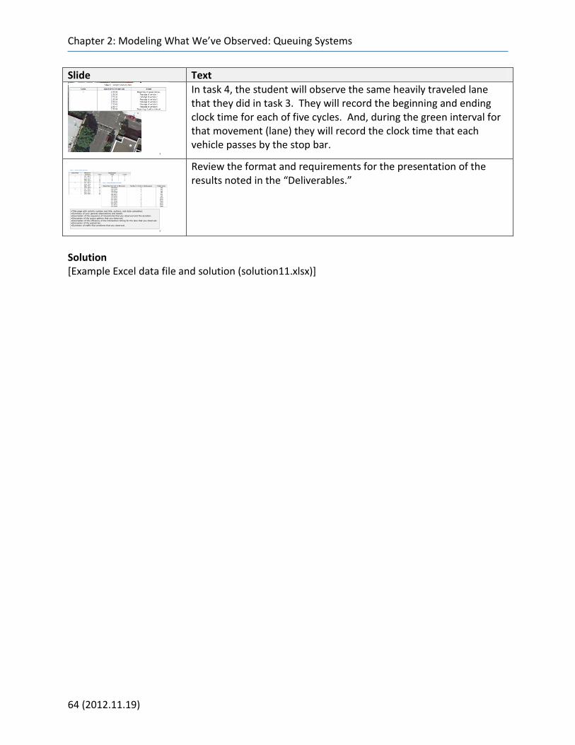
In task 4, the student will observe the same heavily traveled lane that they did in task 3. They will record the beginning and ending clock time for each of five cycles. And, during the green interval for that movement (lane) they will record the clock time that each vehicle passes by the stop bar.

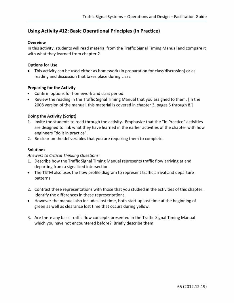
Review the format and requirements for the presentation of the results noted in the “Deliverables.”

Solution [Example Excel data file and solution (solution11.xlsx)]

5

2

•Title page with activity number and title, authors, and date completed.•Summary of your general observations and sketch.•Description of the sequence of movements that you observed and the duration.•Discussion of the queue pattern that you observed.•Description of the efficiency of the intersection timing for the lane that you observed.•Discussion of the pedestrian.•Summary of traffic flow problems that you observed.


65 (2012.12.19)

Using Activity #12: Basic Operational Principles (In Practice) Overview In this activity, students will read material from the Traffic Signal Timing Manual and compare it with what they learned from chapter 2. Options for Use

This activity can be used either as homework (in preparation for class discussion) or as reading and discussion that takes place during class.

Preparing for the Activity

Confirm options for homework and class period.

Review the reading in the Traffic Signal Timing Manual that you assigned to them. [In the 2008 version of the manual, this material is covered in chapter 3, pages 5 through 8.]

Doing the Activity (Script) 1. Invite the students to read through the activity. Emphasize that the “In Practice” activities

are designed to link what they have learned in the earlier activities of the chapter with how engineers “do it in practice”.

2. Be clear on the deliverables that you are requiring them to complete. Solutions Answers to Critical Thinking Questions: 1. Describe how the Traffic Signal Timing Manual represents traffic flow arriving at and

departing from a signalized intersection.

The TSTM also uses the flow profile diagram to represent traffic arrival and departure patterns.

2. Contrast these representations with those that you studied in the activities of this chapter.

Identify the differences in these representations.

However the manual also includes lost time, both start up lost time at the beginning of green as well as clearance lost time that occurs during yellow.

3. Are there any basic traffic flow concepts presented in the Traffic Signal Timing Manual

which you have not encountered before? Briefly describe them.


66 (2012.11.19)

Documents

Assessment 30 min 30 min 50 minutes 30 min 50 …...intersection using what we call a D/D/1 queuing model. We are assuming deterministic arrivals, deterministic service pattern, and