Embed Size (px)
Citation preview

Assessing the Hydrodynamic and Economic
Impacts of Biofouling on the Hull of Surface
Vessels Using Numerical Methods
by
Letchi Evrard Quentin Anoman
Diplome de l’Ecole Royale NavaleMechanical Engineering
Ecole Royale Navale2011
A thesissubmitted to the College of Engineering at
Florida Institute of Technologyin partial fulfillment of the requirements
for the degree of
Master of Sciencein
Ocean Engineering
Melbourne, FloridaApril 2017

COPYRIGHT
In presenting this thesis in partial fulfillment of the requirements for an advanceddegree at Florida institute of technology, I agree that the library shall make itfreely available for reference and study. I further agree that permission forcopying of this thesis for scholarly purposes may be granted by the Head of mydepartment or by his or her representatives. It is understood that copying ofthis thesis for financial gain shall not be allowed without my written permission.
Letchi Anoman
Department of Ocean Engineering and SciencesFlorida Institute of TechnologyMelbourne, Florida
April 20th, 2017
c© Copyright 2017 Letchi Evrard Quentin AnomanAll Rights Reserved
Signature

We the undersigned committee hereby recommendthat the attached document be accepted as fulfilling in
part the requirements for the degree ofMaster of Science in Ocean Engineering.
“Assessing the Hydrodynamic and Economic Impacts of Biofouling on theHull of Surface Vessels Using Numerical Methods”,
a thesis by Letchi Evrard Quentin Anoman
Prasanta K. Sahoo, Ph.D.Associate Professor, Ocean Engineering and SciencesCommittee Chair
Chelakara Subramanian, Ph.D.Professor and Chair, Mechanical and Aerospace Engineering
Geoffrey Swain, Ph.D.Professor, Ocean Engineering and Sciences
Ronnal Reichard, Ph.D.Professor, Ocean Engineering and Sciences
Stephen Wood, Ph.D.Department Head, Ocean Engineering and Sciences

Abstract
TITLE: Assessing the Hydrodynamic and Economic Impacts of
Biofouling on the Hull of Surface Vessels Using Numer-
ical Methods
AUTHOR: Letchi Evrard Quentin Anoman
MAJOR ADVISOR: Prasanta K. Sahoo, Ph.D.
Marine fouling on the hull of surface vessels is a topic of increasing impor-
tance in the maritime field for its environmental and financial impacts. Recent
research developments have introduced mathematical models dealing with the
frictional resistance associated with fouling, thus enabling to single out their
impact on ship hydrodynamics. Herein, two implementations of these models
are presented.
The first implementation used Computational Fluid Dynamics to assess the
additional drag induced by fouling for a specific ship model. With the software
STAR CCM+, Reynolds Averaged Navier-Stokes equations have been used to
model turbulence, wall laws parameters have been adapted to suit a Colebrook-
type engineering roughness function, and a hybrid wall treatment captures the
flow near the wall. Full details of the simulation set-up are given.
The second implementation used turbulent flow similarity scaling laws in a
MATLAB code to predict the added resistance of ships due to biofouling and the
associated costs. With flexibility in mind, the code has been designed to account
for the singularity of each context based on at least one in-situ observation of the
fouling condition. Through a hypothetical, yet realistic scenario, it is shown that
iii

it enables proactive management by indicating when the cumulative penalty of
fouling is no longer tolerable from a financial standpoint.
The results of both implementations were validated against experimental data
found in the literature. Prediction of the additional drag caused by fouling on
a frigate showed excellent agreement of both methods.
iv

Nomenclature
Latin Symbols
1 + k1 Form factor
AT Transom area
ABT Transverse bulb area
B Log-law intercept
CA Correlation allowance
CB Block coefficient
Cc Cleaning cost
CF Frictional resistance coefficient
Cf Local skin friction coefficient
CM Midship area coefficient
CP Prismatic coefficient
CR Residuary resistance coefficient
CT Total resistance coefficient
CV Viscous resistance coefficient
CW Wave resistance coefficient
v

Cfuel Cumulative added fuel cost
cfuel Fuel price
CWP Waterplane area coefficient
E Wall function coefficient
Fn Froude number
FC Cumulative extra fuel consumption
g Acceleration due to gravity
hB Center of bulb area above keel line
iE half angle of entrance
K Turbulent kinetic energy
k Roughness height
KF Cumulative added power
ks Sand grain roughness height
L Length of ship
LR Length of run
LWL Length at waterline
lcb longitudinal center of buoyancy forward of 0.5L as
a percentage of L
PB Brake power
PE Effective power
Ra Centerline averaged roughness height
Rn Reynolds number
vi

RT Total resistance coefficient
Rt Maximum peak to trough roughness height
RW Wave resistance
Rt50 Maximum peak to trough roughness height over a
length of 50mm
S Wetted surface area
T Threshold time
TF Draft at forward perpendicular
Tsea Time spent at sea
U Velocity
Ue Freestream velocity
Uτ Friction velocity
Greek Symbols
∆U+ Roughness function
δ Boundary layer thickness
ε Turbulent energy dissipation rate
η Efficiency of the propulsion line
κ Von Karman constant
µ Dynamic viscosity
∇ Volumetric displacement
ν Kinematic viscosity
ω Turbulent specific energy dissipation rate
vii

ρ Density of fluid
τ Shear stress
τw Wall shear stress
Superscripts
+ Normalized variable
Subscripts
clean Clean, newly coated
exp experimental
r rough
sm smooth
Acronyms
ABS American Bureau of Shipping
AF Antifouling
ATTC American Towing Tank Confe/rence
BMT British Maritime Technology
CFD Computational Fluid Dynamics
DNS Direct Numerical Simulation
DOF Degrees of freedom
EHP Estimated Hull Performance
EVM Eddy-viscosity Model
viii

GHG Greenhouse Gas
IFO Intermediate Fuel Oil
IMO International Maritime Organization
IPPIC International Paint and Printing Ink Council
ITTC International Towing Tank Conference
LES Large Eddy Simulation
MEPC Marine Environment Protection Committee
NSTM Naval Ships’ Technical Manual
RANS Reynolds Averaged Navier-Stokes
ROV Remotely Operated Vehicle
SFOC Specific Fuel Oil Consumption of Engine
SPC Self Polishing Copolymer
SST Shear Stress Transport
TBT Tributyl Tin
USN United States Navy
VOF Volume of Fluid
WHOI Woods Hole Oceanographic Institution
ix

Contents
Abstract iii
Nomenclature v
List of Figures xiii
List of Tables xvi
Acknowledgments xvii
Dedication xviii
1 Introduction 1
1.1 Motivation . . . . . . . . . . . . . . . . . . . . . . . . . . . . . . 1
1.2 The Biofouling Phenomenon . . . . . . . . . . . . . . . . . . . . 2
1.3 Biofouling Management . . . . . . . . . . . . . . . . . . . . . . 4
2 Theoretical Background 6
2.1 Computational Fluid Dynamics . . . . . . . . . . . . . . . . . . 6
2.2 Prediction of the Required Propulsive Power of Ships . . . . . . 10
2.3 Boundary Layer Theory . . . . . . . . . . . . . . . . . . . . . . 13
2.4 Turbulent Flow Similarity and Scaling Law . . . . . . . . . . . . 14
2.5 Roughness Functions for Antifouling Coatings and Fouled Surfaces 17
3 CFD Modeling 21
3.1 Simulation Set-up . . . . . . . . . . . . . . . . . . . . . . . . . . 21
3.1.1 Geometry . . . . . . . . . . . . . . . . . . . . . . . . . . 21
x

3.1.2 Computational domain . . . . . . . . . . . . . . . . . . . 23
3.1.3 Meshing . . . . . . . . . . . . . . . . . . . . . . . . . . . 23
3.1.4 Physical models . . . . . . . . . . . . . . . . . . . . . . . 29
3.1.5 Boundary conditions . . . . . . . . . . . . . . . . . . . . 29
3.1.6 Wall laws . . . . . . . . . . . . . . . . . . . . . . . . . . 30
3.1.7 Solvers . . . . . . . . . . . . . . . . . . . . . . . . . . . . 32
3.1.8 Stopping Criteria . . . . . . . . . . . . . . . . . . . . . . 33
3.2 Convergence Study . . . . . . . . . . . . . . . . . . . . . . . . . 34
3.2.1 Mesh . . . . . . . . . . . . . . . . . . . . . . . . . . . . . 34
3.2.2 Time step . . . . . . . . . . . . . . . . . . . . . . . . . . 37
3.2.3 Wall treatment . . . . . . . . . . . . . . . . . . . . . . . 37
3.3 Validation Study . . . . . . . . . . . . . . . . . . . . . . . . . . 41
3.4 Results/Prediction . . . . . . . . . . . . . . . . . . . . . . . . . 41
4 MATLAB Code 47
4.1 Procedure to Find Added Power Due to Fouling . . . . . . . . . 47
4.2 Calibration and Validation of the Code . . . . . . . . . . . . . . 49
4.3 Biofouling Tolerability Prediction . . . . . . . . . . . . . . . . . 53
4.3.1 Method . . . . . . . . . . . . . . . . . . . . . . . . . . . 53
4.3.2 Results . . . . . . . . . . . . . . . . . . . . . . . . . . . . 56
4.4 Percent Fouling Penalty Calculation . . . . . . . . . . . . . . . . 63
4.4.1 Method . . . . . . . . . . . . . . . . . . . . . . . . . . . 63
4.4.2 Variability/Similarity of Fouling Penalty with Ship Types 64
4.5 Discussion . . . . . . . . . . . . . . . . . . . . . . . . . . . . . . 69
5 Conclusion 71
6 Recommendations for future research 73
References 75
A Calculation of wave resistance 80
B Ship Particulars 83
C Description of Simulation Models (CD-ADAPCO, 2017) 84
xi

D CFD validation study 87
xii

List of Figures
1.1 Example of slime fouling on a ship’s hull, ABS (2013) . . . . . . 3
2.1 General sequence of operations in a STAR CCM+ analysis (CD-
ADAPCO, 2017) . . . . . . . . . . . . . . . . . . . . . . . . . . 8
2.2 Direct Numerical Simulation (Cengel and Cimbala, 2006) . . . . 9
2.3 Large Eddy Simulation (Cengel and Cimbala, 2006) . . . . . . . 9
2.4 Reynolds Averaged Navier-Stokes Simulation (Cengel and Cim-
bala, 2006) . . . . . . . . . . . . . . . . . . . . . . . . . . . . . . 9
2.5 Law of the wall plot for a turbulent boundary layer. K is the Von
Karman constant, E ′ is the ratio of the wall function coefficient
by the roughness function (CD-ADAPCO, 2017) . . . . . . . . . 14
2.6 The effect of roughness on the law of the wall, (Schultz and Swain,
2000) . . . . . . . . . . . . . . . . . . . . . . . . . . . . . . . . . 15
2.7 Graphical representation of Granville similarity scaling law (Schultz,
2007) . . . . . . . . . . . . . . . . . . . . . . . . . . . . . . . . . 17
2.8 Fouling rating (NSTM, 2006) . . . . . . . . . . . . . . . . . . . 20
3.1 Plate geometry . . . . . . . . . . . . . . . . . . . . . . . . . . . 22
3.2 Perspective view of domain . . . . . . . . . . . . . . . . . . . . . 23
3.3 Plate refinements . . . . . . . . . . . . . . . . . . . . . . . . . . 24
3.4 Very thin free surface refinement . . . . . . . . . . . . . . . . . 24
3.5 Thin free surface refinement . . . . . . . . . . . . . . . . . . . . 25
3.6 Thick free surface refinement . . . . . . . . . . . . . . . . . . . . 25
3.7 Wake refinement . . . . . . . . . . . . . . . . . . . . . . . . . . 26
3.8 Wakebox refinement . . . . . . . . . . . . . . . . . . . . . . . . 26
xiii

3.9 Plate mesh . . . . . . . . . . . . . . . . . . . . . . . . . . . . . . 27
3.10 Mesh perspective view . . . . . . . . . . . . . . . . . . . . . . . 27
3.11 Mesh side view . . . . . . . . . . . . . . . . . . . . . . . . . . . 28
3.12 Mesh top view . . . . . . . . . . . . . . . . . . . . . . . . . . . . 28
3.13 External boundaries . . . . . . . . . . . . . . . . . . . . . . . . 30
3.14 Convergence of simulations in fouled condition . . . . . . . . . . 33
3.15 Shear drag monitor plot . . . . . . . . . . . . . . . . . . . . . . 35
3.16 Shear drag in the last 12 seconds . . . . . . . . . . . . . . . . . 36
3.17 Improper mesh transition (base size=0.05m) . . . . . . . . . . . 36
3.18 Improper mesh topology (base size=0.12m) . . . . . . . . . . . . 37
3.19 Time convergence plot . . . . . . . . . . . . . . . . . . . . . . . 38
3.20 Initial wall cell size requirement for each wall treatment model
(CD-ADAPCO, 2017) . . . . . . . . . . . . . . . . . . . . . . . 40
3.21 Hull form of a frigate (MAXSURF) . . . . . . . . . . . . . . . . 43
3.22 Domain view for the prediction study . . . . . . . . . . . . . . . 43
3.23 Overall mesh for the prediction study . . . . . . . . . . . . . . . 44
3.24 Frigate mesh . . . . . . . . . . . . . . . . . . . . . . . . . . . . . 44
3.25 Variation of resistance with speed and fouling condition . . . . . 45
3.26 Variation of resistance coefficients with speed and fouling condition 46
4.1 Comparison of ITTC, Schoenherr friction lines and experimental
CF (experimental data from Schultz (2004)) . . . . . . . . . . . 49
4.2 Comparison of experimental and calculated CF (experimental
data from Schultz (2004)) . . . . . . . . . . . . . . . . . . . . . 51
4.3 Comparison of experimental and calculated CF (experimental
data from Kempf (1937)) . . . . . . . . . . . . . . . . . . . . . . 51
4.4 Comparison of resistance predictions of MATLAB against CFD
for a frigate (wave resistance calculated as per Holtrop and Men-
nen (1982) . . . . . . . . . . . . . . . . . . . . . . . . . . . . . . 52
4.5 Summary of the biofouling tolerability prediction method for ships 55
4.6 Cruise ship model (MAXSURF) . . . . . . . . . . . . . . . . . . 56
4.7 Percent distribution of fouling on fouling release coating observed
on 5 cruise ships (Koka, 2014) . . . . . . . . . . . . . . . . . . . 58
4.8 Added power and cumulative extra fuel cost for a cruise ship . . 58
xiv

4.9 Added daily fuel consumption and costs for a cruise ship . . . . 59
4.10 Hull form of a cruise ship (MAXSURF) . . . . . . . . . . . . . . 60
4.11 Hull form of a frigate (MAXSURF) . . . . . . . . . . . . . . . . 60
4.12 Hull form of a trawler (MAXSURF) . . . . . . . . . . . . . . . . 61
4.13 Fouling tolerability analysis for a cruise ship . . . . . . . . . . . 61
4.14 Fouling tolerability analysis for a frigate . . . . . . . . . . . . . 62
4.15 Fouling tolerability analysis for a trawler . . . . . . . . . . . . . 62
4.16 Percent penalty for various fouling conditions and ship types . . 66
4.17 Percent penalty vs Fn for various fouling conditions and ship types 67
4.18 Scaled percent penalty vs Fn for various fouling conditions and
ship types . . . . . . . . . . . . . . . . . . . . . . . . . . . . . . 68
D.1 Wall shear stress τw over the plate (Pa = N/m2) . . . . . . . . 87
D.2 Friction velocity Uτ over the plate . . . . . . . . . . . . . . . . . 88
D.3 Roughness Reynolds number k+ over the plate . . . . . . . . . . 88
D.4 Non-dimensional distance from the wall y+ . . . . . . . . . . . . 89
D.5 Wall Y+ based on first cell size . . . . . . . . . . . . . . . . . . 89
xv

List of Tables
1.1 Classification of major fouling species, Koka (2014) . . . . . . . 4
2.1 Ship types and parameters range (Holtrop and Mennen, 1982;
Molland et al., 2011) . . . . . . . . . . . . . . . . . . . . . . . . 12
2.2 Fouling condition of fouled plates, adapted from Schultz (2004) . 19
2.3 Fouling reference table, adapted from Swain and Lund (2016);
Schultz (2007); NSTM (2006) . . . . . . . . . . . . . . . . . . . 19
3.1 Boundary conditions . . . . . . . . . . . . . . . . . . . . . . . . 29
3.2 Mesh convergence study . . . . . . . . . . . . . . . . . . . . . . 35
3.3 Time convergence study . . . . . . . . . . . . . . . . . . . . . . 38
3.4 Initial wall cell size study (fouled Silicone 1) . . . . . . . . . . . 39
3.5 Initial wall cell size study (unfouled Silicone 1) . . . . . . . . . . 40
3.6 Comparison of experimental (Schultz, 2004) vs simulated CF at
Rn = 2.8 · 106 . . . . . . . . . . . . . . . . . . . . . . . . . . . . 42
4.1 Summary of assumptions for the Cruise ship prediction . . . . . 57
4.2 Fouling condition . . . . . . . . . . . . . . . . . . . . . . . . . . 57
4.3 Ship particulars . . . . . . . . . . . . . . . . . . . . . . . . . . . 60
B.1 Ship particulars . . . . . . . . . . . . . . . . . . . . . . . . . . . 83
C.1 Meshers . . . . . . . . . . . . . . . . . . . . . . . . . . . . . . . 84
C.2 Physical models . . . . . . . . . . . . . . . . . . . . . . . . . . . 85
C.3 Solvers . . . . . . . . . . . . . . . . . . . . . . . . . . . . . . . . 86
xvi

Acknowledgements
I would like to express my deepest gratitude to the Fulbright Program Division,
who gratefully sponsored my entire master’s program. My sincere thankfulness,
likewise, goes to the Navy of Cote d’Ivoire for allowing and supporting my
educational endeavor.
Also, I would like to thank Dr. Prasanta Sahoo for his guidance throughout the
duration of the master’s program. In particular, his assistance in the completion
of the current thesis is greatly appreciated.
My appreciation also goes to Dr. Geoffrey Swain who devoted much of his
time to answering my questions. Thanks also to Dr. Ronnal Reichard and Dr.
Chelakara Subramanian for their encouragement and time.
The help of Yipeng Pan, Lin Du, Johanna Evans, Vaibhav Aribenchi, Karthik
Avala, Bhanu Prakash and Agu Nnamdi is gratefully acknowledged.
xvii

Dedication
To God, the source of all grace and knowledge,
To my loving wife, for her continuous and unfailing support, despite having to
bear the pain of much distance,
And to our baby, growing healthily in her womb, to whom I hope to be a good
father.
xviii

Chapter 1
Introduction
1.1 Motivation
Marine fouling or biofouling can be defined as the settlement and growth of
marine organisms on a submerged hull surface. When these organisms attach
to the hull of a ship, they increase the roughness of the hull surface. As a
result, the viscous resistance and the required propulsive power of the ship
increase causing an environmental as well as a financial impact.
The International Paint and Printing Ink Council (IPPIC) reported to the In-
ternational Maritime Organization (IMO) that fouling free vessels can offer a
significant contribution to the reduction of greenhouse gas (GHG) emissions
from ships (IPPIC, 2010). The report estimates that if the global fleet were
to have only a thin layer of slime, 134 million tonnes of extra CO2 would be
emitted into the atmosphere by 2020. Moreover, marine fouling poses a threat
to the environment through the transfer of invasive species. For this reason,
several countries have adopted regulations and the IMO published guidelines to
1
address the issue (IMO, 2011).
Haslbeck and Bohlander (1992) asserted that nearly 20% of the United States
Navy (USN) Fleet propulsive fuel bill is spent annually to overcome the addi-
tional drag due to fouling. Schultz et al. (2011) estimated that the overall cost
for the USN associated with fouling for the entire DDG-51 class of destroyer is
nearly $1b over a 15-year period. Kattan et al. (2015) asserted that fuel con-
sumption may account for 50% or more of a vessel operating costs. Clearly, this
ratio will further increase if the resistance of the vessel is affected by biofouling.
Considering these facts, the marine industry devotes much efforts to effectively
manage biofouling through prevention, monitoring and cleaning.
It is of interest to ship researchers to be able to simulate the effects of bio-
fouling on the hull of surface vessels. A logical extension of this capability
is, among others, the ability to predict when it is desirable to undertake hull
cleaning from an economic perspective. Therefore, the current study presents a
Computational Fluid Dynamics (CFD) implementation of existing mathemati-
cal models to capture the drag induced by biofouling. A numerical code is also
presented which provides an alternative way of calculating the added power and
associated costs of biofouling on a vessel under calm water conditions. This lat-
ter tool is flexible enough to give an estimate of when the cumulative penalty
of fouling overcomes the cleaning cost.
1.2 The Biofouling Phenomenon
Biofouling occurs within minutes after a body is submerged with the formation
of an organic film. This is followed by the colonization of bacterial slimes and
2

diatoms. Within weeks, larger organisms such as barnacles and macro algae
develop. These have a greater impact on a ship’s resistance.
The fouling community is composed of animals (barnacles, hydroids, mollusks,
etc.), and plants (brown algae, green algae, etc.). It is well known that the extent
and severity of biofouling depends on several factors such as temperature, water
salinity, light, nutrient availability and other environmental conditions (WHOI
and USN, 1952; Hunsucker et al., 2014). Vessels operating at low speeds or
being at berth for extended periods are more likely to become fouled.
A classification of major fouling species is presented in Table 1.1.
Figure 1.1: Example of slime fouling on a ship’s hull, ABS (2013)
3

Table 1.1: Classification of major fouling species, Koka (2014)
Group Description
Slime Biofilms containing bacteria, fungi, unicellular organisms, di-atoms, initial algal germination, and low form algae
Weed Green or red mats of filamentous plants (e.g. Ulva spp., Ecto-carpus)
Soft fouling Low form plants and animals that form soft growths up to 150mm in diameter
Shell fouling Hard shelled crustacean worms and mollusks including barna-cles, tubeworms and oysters
1.3 Biofouling Management
Typically, biofouling management is addressed through prevention, monitoring
and cleaning.
Prevention of marine fouling on the underwater hull of a vessel is made by
antifouling coating systems. Since the ban by the IMO of organotin-based
systems (notably the well-known tributyl-tin or TBT), the maritime industry
has been striving to find an effective replacement. Modern coating systems can
be classified into biocide-based and biocide free systems. It should be noted that
they are also commonly divided into the following groups which reflect more the
technology used: control depletion polymers (CDP), self-polishing co-polymers
(SPC), foul release coatings (FRC), and combination technologies.
Monitoring the state of an antifouling coating system can be achieved by mea-
suring fuel consumption on regularly spaced time intervals. Yet, such a task
is not an easy one as many factors influence data collection: weather (wind
4

and waves), sea currents, temperature and salinity, ship’s loading, etc. Munk
et al. (2009) gives a more thorough analysis of in-service vessel performance
monitoring and notes that so far there is no standardized method to measure
vessel performance. A simpler approach to assess the fouling condition of a hull
is by a visual inspection using a diver or Remotely Operated Vehicle (ROV)
with a waterproof camera. Notwithstanding the advantages of this method, it
is regarded as subjective.
If the hull is judged as excessively fouled, several cleaning options are available.
In the first option, waterborne cleaning can be carried out. It has the advantage
of not affecting much the ship’s availability. As noted by the USN Naval Ships’
Technical Manual (NSTM, 2006), “total ship performance and fleet capability
can be enhanced by waterborne cleaning and maintenance”. The manual speci-
fies when cleaning should occur and defines several types of waterborne cleaning
depending on the sections to be cleaned: full cleaning, interim cleaning and par-
tial cleaning. The US Navy is also investigating a proactive hull maintenance
procedure known as grooming (Tribou and Swain, 2010). This is defined as
cleaning with soft tools before fouling becomes established (for example, hull
grooming of a slimed hull). In the second option, cleaning may take place dur-
ing dry-docking. In this case, a full or partial blast of the hull plus recoating
are possible.
More detailed reviews of biofouling management are developed by INTER-
TANKO (2016) and Kattan et al. (2015).
5

Chapter 2
Theoretical Background
2.1 Computational Fluid Dynamics
Computational Fluid Dynamics (CFD) is the field of study that uses computers
and numerical methods to solve problems involving fluid flow. Three main
governing equations are solved (Cebeci et al., 2005):
• Continuity equation (conservation of mass)
∂ρ
∂t+∇(ρu) = 0 (2.1)
• Momentum equation (Navier-Stokes)
∂u
∂t+ (u · ∇)u = −1
ρ∇p+
1
ρ∇τ +
1
ρF (2.2)
• Energy equation (first law of thermodynamics)
∂E
∂t+∇(E · u) = −∇q +∇(Πij · u) + F · u + SE (2.3)
6

Here, u is the velocity vector, p is the pressure, τ is the shear stress tensor, F is
the resultant of external body forces, E is the total energy per unit volume, q
is the heat flux, SE is an energy source per unit volume. Πij is the stress tensor
given as the sum of normal and shear stresses, Πij = −pδij + τij where δij is the
Kronecker delta function (δij = 1 if i = j, δij = 0 if i 6= j) for i, j = 1, 2, 3.
Typically, a CFD simulation involves three stages:
• Pre-processing: at this stage, the problem is formulated by creating the
geometry, selecting the applicable equations, defining the boundary con-
ditions and constructing the mesh;
• Solving: the CFD package discretizes and solves the equations over the
elementary volumes of the mesh;
• Post-processing: the results are visualized and analyzed.
An overview of the simulation workflow in STAR CCM+ is presented in Figure
2.1.
Turbulence is one of the many complex engineering fluid flow problems that
CFD endeavors to tackle. As in most engineering applications, the flow along
the hull of a ship (even more a fouled hull) is turbulent. Turbulence can be mod-
elled by Direct Numerical Simulation (DNS), Large Eddy Simulation (LES) or
Reynolds Averaged Navier-Stokes (RANS) equations (Figures 2.2 to 2.4). While
DNS solves for the exact governing equations with an extremely fine grid spac-
ing, RANS equations provide closure relations by an averaging process called
Reynolds averaging. This process, which is computationally more convenient,
considers any instantaneous flow variable as the sum of a mean and a fluctuating
variable. For example, the instantaneous velocity would be u = u+u′, where u
7

Figure 2.1: General sequence of operations in a STAR CCM+ analysis (CD-ADAPCO, 2017)
and u′ denote respectively the mean velocity and the fluctuating velocity. LES
is a combination of both DNS and RANS with an attempt to solve only for the
largest eddies.
8

Figure 2.2: Direct Numerical Simulation (Cengel and Cimbala, 2006)
Figure 2.3: Large Eddy Simulation (Cengel and Cimbala, 2006)
Figure 2.4: Reynolds Averaged Navier-Stokes Simulation (Cengel and Cimbala,2006)
9

The Reynolds averaging process gives rise to Reynolds stresses (or turbulent
stresses) such that the shear stress becomes the sum of viscous and turbulent
components i.e.:
τij = µ(∂ui
∂xj+∂uj
∂xi) + τij,turbulent (2.4)
Where τij,turbulent = −ρuiuj.
As per the eddy-viscosity model (EVM) assumption,
τij,turbulent = µt(∂ui
∂xj+∂uj
∂xi)− 2
3ρKδij (2.5)
Here, µt is the eddy viscosity (or turbulent viscosity) which may be modelled
in terms of the turbulent kinetic energy K and the turbulent energy dissipation
rate ε (K−ε model) or the turbulent kinetic energy K and the turbulent specific
energy dissipation rate ω (K − ω model).
2.2 Prediction of the Required Propulsive Power
of Ships
The motion of a ship in seaway is altered by fluid forces opposing the motion.
These forces constitute the resistance of the ship. They can be divided into two
main components: the frictional resistance, due to tangential shear stresses,
and the residuary resistance, the major component of which is wave resistance.
William Froude postulated that the wave resistance of a ship could be inferred
from a geometrically similar model whereas frictional resistance is a function of
the wetted surface area and speed.
Under the assumption that the frictional resistance of a ship is equal to that of an
10

equivalent flat plate (i.e. ship and plates having the same wetted surface area),
the American Towing Tank Conference (ATTC) of 1947 adopted the Schoenherr
friction line (Equation 2.6) to determine the frictional resistance coefficient CF
of a ship. In 1957, the International Towing Tank Conference (ITTC) adopted
the ITTC-1957 model-ship correlation line (Equation 2.7) which was found to
be a more accurate prediction of CF for ships.
log(Rn · CF ) =0.242√CF
(2.6)
CF =0.075
(logRn − 2)2(2.7)
Here, Rn is the Reynolds number of the ship given as Rn = U ·Lν
where U and
L are respectively the velocity and length of the ship, and ν is the kinematic
viscosity of the fluid (typically seawater). There is a good agreement between
both friction lines for Rn > 108.
According to the 2D extrapolation procedure recommended by the ITTC-1957,
the effective power required to move a ship at speed U is:
PE = RT · U (2.8)
RT is the total resistance of the ship given as RT = 12ρCTSU
2, where ρ is the
density of the fluid, S is the wetted surface area of the ship and CT is the coeffi-
cient of total resistance. The latter is expressed as CT = CF +CR+CA where the
residuary resistance coefficient CR is typically determined from model testing
or empirical formulations, and the correlation allowance CA is an incremental
resistance coefficient used to account for the paint/surface roughness of the new
11

ship as built.
It should be noted that the procedure was further improved by the adoption of
a 3D extrapolation procedure known as the 1978-ITTC performance prediction
method (Oosterveld, 1978). The major improvement is the introduction of a
form factor (1 + k1) to take into account the three-dimensional shape of a ship
such that CV = (1 + k1)CF and CT = CV + CR + CA. The 3D extrapolation
procedure also suggests methods for the calculation of appendage resistance.
Finally, the engine power or brake power PB, i.e. the power delivered at engine
coupling can be expressed as:
PB =PEη
(2.9)
Where η is the efficiency of the entire propulsion system (combining quasi-
propulsive efficiency, shaft efficiency, and gear efficiency).
Holtrop and Mennen (1982) and Holtrop (1984) proposed regression equations
for the calculation of the wave resistance of ships (see Appendix A). The recom-
mended ship types and parameter ranges are listed in Table 2.1. Here, Fn, CP
and B are respectively the Froude number (Fn = U√gL
), the prismatic coefficient
and the maximum beam of the vessel.
Table 2.1: Ship types and parameters range (Holtrop and Mennen, 1982; Mol-land et al., 2011)
Ship type Fn,max CP L/B
Tankers and bulk carriers 0.24 0.73-0.85 5.1-7.1
General cargo 0.30 0.58-0.72 5.3-8.0
Fishing vessels, tugs 0.38 0.55-0.65 3.9-6.3
Container ships, frigates 0.45 0.55-0.67 6.0-9.5
12

2.3 Boundary Layer Theory
The boundary layer can be defined as “the area closest to the hull in which
the fluid is impeded as a result of its viscosity” (Schultz and Swain, 2000).
Along the hull surface of a ship, the boundary layer is mostly turbulent, i.e. the
velocity and pressure distribution have random fluctuations in space and time.
A turbulent boundary layer can be divided into the following (Figure 2.5):
• the inner region composed of:
– the viscous (or linear) sublayer where U+ = y+
– the log-law layer, Schlichting (1968), where
U+ =1
κln(y+) +B −∆U+ (2.10)
– the buffer layer which is a transitional layer between the viscous
sublayer and the log-law layer
• the outer region where the local mean velocity is governed by the velocity-
defect law U+e − U+ = g(y
δ)
U+, U+e , y+ and the roughness Reynolds number k+ are normalized quantities
given as U+ = UUτ
, U+e = Ue
Uτ, y+ = yUτ
ν, and k+ = kUτ
νwhere Ue is the velocity
at the edge of the boundary layer, Uτ =√
τwρ
is the friction velocity, y is the
offset distance from the boundary i.e. the wall, and k is the roughness height
(note that k is an artificial parameter used to assess roughness effects, it is
not a physical measurement). κ is the Von Karman constant, B is the log-law
intercept for smooth walls, δ is the boundary layer thickness, and g denotes the
13

velocity-defect function which is thought to be universal. ∆U+ is the roughness
function which accounts for the effects of roughness in the flow field (Figure
2.6).
Figure 2.5: Law of the wall plot for a turbulent boundary layer. K is the VonKarman constant, E ′ is the ratio of the wall function coefficient by the roughnessfunction (CD-ADAPCO, 2017)
2.4 Turbulent Flow Similarity and Scaling Law
Granville (1958) postulated that “the frictional effects of any particular rough-
ness may be considered defined when ∆U+ is experimentally determined as a
function of k+”. He further argued that “if a representative sample of the rough
surface can be obtained on a test plate, it is then possible to make full-scale
predictions for any arbitrary roughness configuration without regard to geomet-
rical characterization”. Then, he developed a scaling procedure based on the
14

Figure 2.6: The effect of roughness on the law of the wall, (Schultz and Swain,2000)
following relationships:
logRn = logRn,sm +(∆U+ −∆U+
sm)κ
ln 10(2.11)
logRn = log(LUτν
)− log
√CF2
+
√CF2
κ · ln(10)(2.12)
logRn,2 = logRn,1 + log(L2
L1
) (2.13)
Equation 2.11, valid at constant CF , means that the frictional curve of a rough
plate is offset by a distance ∆U+·κln (10)
from the smooth curve; Equation 2.12 means
15
that logRn can be plotted as a function of CF for a given viscous length scale
Uτν
and plate length; Equation 2.13 means that logRn of plate 2 is a distance
log L2
L1from logRn of plate 1 for a given roughness height and a given viscous
length scale.
Therefore, given two plates of respective lengths L1 and L2, with the same
roughness, if the velocity of the second plate is known which means Rn,2 is
known , and the roughness functions obtained experimentally with plate 1 are
known, we have (as proposed by Granville (1958)):
(a) Rn,1 is found from Equation 2.13
(b) The viscous length scale is found by solving for Equations 2.11 and 2.12
iteratively,
(c) The rough frictional resistance coefficient curve CF,r is obtained from Equa-
tion 2.11 ,
(d) The rough frictional resistance coefficient of plate 2 is CF2 = CF,r(logRn,2)
.
A graphical representation of the procedure is presented in Figure 2.7. If the
roughness function is defined by an empirical formulation, step (a) can be omit-
ted. It should be noted that a similar iterative procedure has been described by
Schultz (2007). More recently, Monty et al. (2016) also described a similarity
scaling procedure based on momentum equations.
16

Figure 2.7: Graphical representation of Granville similarity scaling law (Schultz,2007)
2.5 Roughness Functions for Antifouling Coat-
ings and Fouled Surfaces
Schultz (2004) tested in a towing tank several coating systems in the unfouled,
fouled, and cleaned conditions with plates of length L = 1.52m (Table 2.2).
Based on his experiments, he found that a Colebrook-type engineering rough-
ness function appropriately characterizes the roughness of unfouled and fouled
coatings:
∆U+ =1
κln(1 + k+) (2.14)
Where
(2.14a) k = 0.17Ra for unfouled coating
(2.14b) k = 0.11Rt for surfaces covered with slime only
17

(2.14c) k = 0.059Rt
√%barnaclefouling for fouled surfaces with barnacles .
Ra and Rt denote physical measurements representing the centerline average
roughness height and the maximum peak to trough roughness height respec-
tively. In the case of fouled surfaces with slime or barnacles, Rt means the slime
thickness or maximum barnacle height respectively. Note that k is an artificial
parameter as it relates to physical measurements as illustrated by Equations
2.14a, 2.14b and 2.14c.
Equation 2.14 exhibited excellent agreement between experimental results and
the formulations for unfouled coatings and coatings covered with barnacles. It
is of note that fouling occurred under static conditions. Even if it is true that
∆U+ would be different for fouling occurring under dynamic conditions (Schultz
et al., 2015; Hunsucker et al., 2016; Zargiel and Swain, 2014), it is a good starting
point for practical evaluation.
If Ra and Rt are not available - which is generally the case in dock-, Table 2.3
can be used as an alternative reference for the determination of the roughness
height k. The NSTM rating is an index based on a visual assessment of the
fouling condition (NSTM, 2006). Figure 2.8 shows examples of such characteri-
zation. Note that ks is the equivalent sand roughness height which conforms to
a Nikuradse-type roughness function (Nikuradse, 1933). Rt50 is Rt for a given
length of 50mm; in the case of fouled surfaces, it implies the likely observable
maximum peak to trough roughness height.
18

Table 2.2: Fouling condition of fouled plates, adapted from Schultz (2004)
Test sur-face
Total foul-ing cover-age (%)
Slime(%)
Hydroids(%)
Barnacles(%)
Height ofhighestbarnacles
Silicone 1 75 10 5 60 ≈ 6mm
Silicone 2 95 15 5 75 ≈ 7mm
Ablativecopper
76 75 0 1 ≈ 5mm
SPC copper 73 65 3 4 ≈ 5mm
SPC TBT 70 70 0 0 NA
Table 2.3: Fouling reference table, adapted from Swain and Lund (2016); Schultz(2007); NSTM (2006)
Condition NSTMFoulingrating
k(µm) ks(µm) Rt50(µm)
Hydraulically smooth 0 0 0 0
Applied AF coating 0 2 30 150
Deteriorated coating 10-20 6 100 300
Light slime 10-20 17 150 400
Moderate slime 20-30 30 210 500
Heavy slime 30 60 300 600
Small calcareous fouling orweed
40-60 320 1000 1000
Medium calcareous fouling 70-80 1000 3000 3000
Heavy calcareous fouling 90-100 3500 10000 10000
19

(a) Fouling rating FR-10 over 100% of area (b) Fouling rating FR-20 over 80% of area
(c) Fouling rating FR-40 over 20% of area (d) Fouling rating FR-60 over 90% of area
(e) Fouling rating FR-70 over 80% of area (f) Fouling rating FR-100 over 50% of area
Figure 2.8: Fouling rating (NSTM, 2006)
20

Chapter 3
CFD Modeling
The CFD package STAR CCM+ was used to simulate the effects of biofouling
by modifying surface roughness parameters. The present study makes use of the
roughness function defined in Equation 2.14. The roughness height k is taken
as per Equations 2.14a to 2.14c or Table 2.3. Here, the advantage is that a
direct correlation between a visual assessment of the fouling severity is utilized
to determine the drag. The results of the simulation are validated against the
experimental data of Schultz (2004). Then, predictions are made for a frigate.
3.1 Simulation Set-up
3.1.1 Geometry
The plate geometry used is in conformity with the experimental setup described
by Schultz (2004). It is a flat plate 1.52m long, 0.76 m wide, and 3.2 mm thick.
The edges are filleted to a radius of 1.6 mm (Figure 3.1). The submerged height
has been set to 0.59 mm.
21
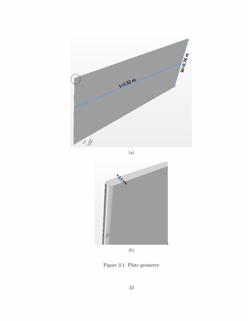
(a)
(b)
Figure 3.1: Plate geometry
22

3.1.2 Computational domain
Figure 3.2: Perspective view of domain
The domain was setup according the recommended practice of CD ADAPCO
for general external flows. The domain extends 2L ahead of the leading edge,
4L behind of the trailing edge, and 2L above the free surface. Its depth and
width were taken equal to the depth and width of the real towing tank (Figure
3.2).
3.1.3 Meshing
A mesh is a discretized representation of the computational domain, which the
physics solvers use to provide a numerical solution (CD-ADAPCO, 2017). As
such, creating the right mesh is an important aspect of the simulation.
23

The meshing models used in this study are the surface remesher, trimmed cell
mesher, and prism layer mesher (refer appendix C for description). Four volu-
metric refinements were set up around the plate (Figure 3.3). Three volumetric
refinements were set up to capture the flow at the free surface (Figures 3.4 to
3.6). Six volumetric refinements were setup to capture the wake (Figures 3.7
and 3.8). The resulting mesh is shown in Figures 3.9 to 3.12.
Figure 3.3: Plate refinements
Figure 3.4: Very thin free surface refinement
24

Figure 3.5: Thin free surface refinement
Figure 3.6: Thick free surface refinement
25

Figure 3.7: Wake refinement
Figure 3.8: Wakebox refinement
26

Figure 3.9: Plate mesh
Figure 3.10: Mesh perspective view
27

Figure 3.11: Mesh side view
Figure 3.12: Mesh top view
28

3.1.4 Physical models
In this study, Reynolds-Averaged Navier-Stokes (RANS) equations have been
used to model turbulence. The Shear Stress Transport (SST) K−ω turbulence
model was used to close the momentum equations. This model provides the
advantages of the K − ω model near the wall and those of the K − ε model
in the far field. It should be noted that a similar study on ships coatings by
Demirel et al. (2014) used the same turbulence model.
3.1.5 Boundary conditions
The simulations were set-up for half a model with a symmetry plane which would
save computational resources without affecting the end result. The Volume
of Fluid (VOF) Damping option has been activated for boundaries that are
sensitive to wave reflection as shown in Table 3.1. VOF Damping is an option
used to reduce numerical instabilities arising from the reflection of waves.
Table 3.1: Boundary conditions
Boundaryname
Boundary type Condition VOF Damp-ing
Tank.Inlet Velocity inlet NA Yes
Tank.Outlet Pressure outlet NA Yes
Tank.Side Wall No slip Yes
Tank.Symmetry Symmetry plane NA No
Tank.Top Wall Slip No
Tank.Bottom Wall No slip No
Plate Wall (smooth/rough) No slip No
29

Figure 3.13: External boundaries
3.1.6 Wall laws
STAR CCM+ uses wall laws describing closely packed uniform sand grain rough-
ness as given by Cebeci and Bradshaw (1977). In particular, the log-law formu-
lation used in Star CCM+ is:
U+ =1
κln(E
′y+) (3.1)
Here, E′= E
fwhere E is the wall function coefficient and f denotes the STAR
CCM+ roughness function given as:
• f = 1 for the hydrodynamically smooth flow regime (k+ < k+sm)
• f = [A(k+−k+smk+r −k+sm
)+Ck+]a for the intermediate flow regime (k+sm < k+ < k+
r )
• f = A+ Ck+ for the fully-rough flow regime (k+ > k+r )
Note that A and C denote coefficients, and the exponent a is a function of k+,
30

k+sm and k+
r .
For the current study, these parameters needed to be adjusted to satisfy the
roughness function proposed by Equation 2.14. To begin with, Equation 2.14
is independent of the flow regime. Therefore, k+sm and k+
r were made very small
so that f would always have the form of the fully rough regime.
The coefficients E, A and C are then found as follows:
• Equalizing Equation 2.10 and 3.1 for smooth walls, we have:
U+ =1
κln(Ey+) =
1
κln(E) +
1
κln(y+) =
1
κln(y+) +B (3.2)
Eliminating redundant terms, we get
1
κln(E) = B (3.3)
And for B = 5.0, κ = 0.42
E = eκ·B = 8.17 (3.4)
• Keeping the fully-rough expression of the STAR CCM+ roughness func-
tion, and equalizing Equations 2.10 and 3.1 for rough flows, we have
U+ =1
κln(
E
fy+) =
1
κln(Ey+)− 1
κln(A+ Ck+) =
1
κln(y+) +B −∆U+
(3.5)
Eliminating redundant terms based on equation 3.2, and replacing by the
31
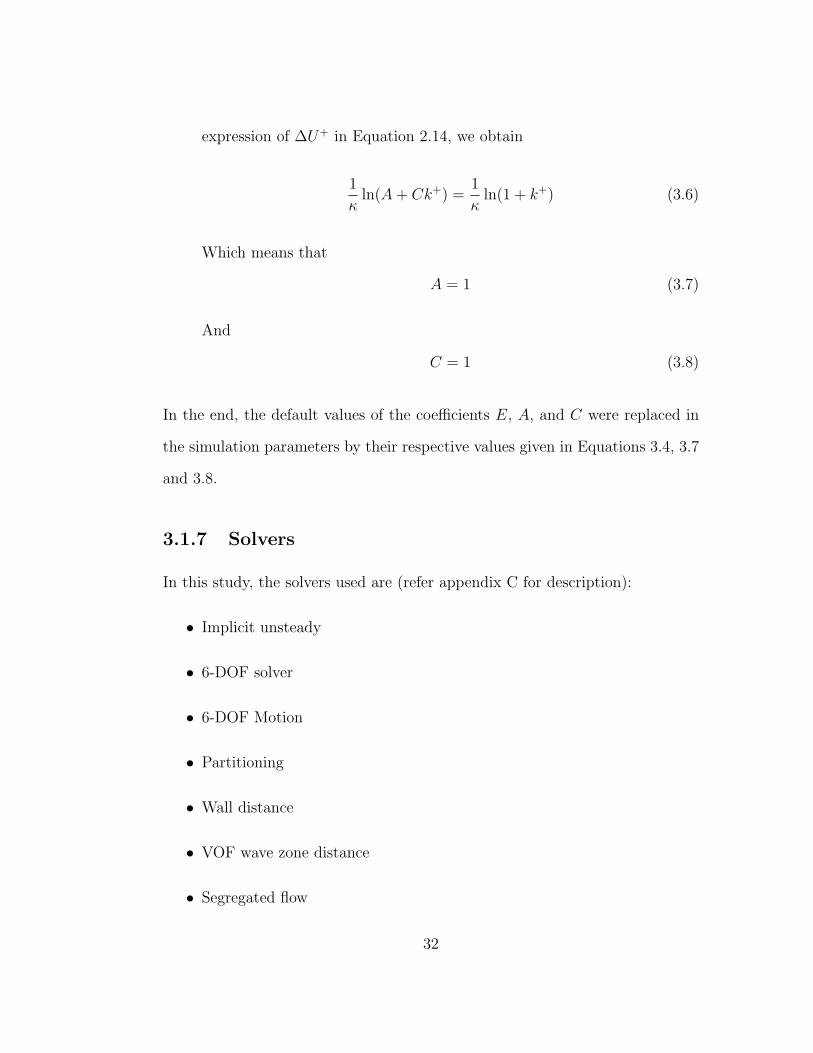
expression of ∆U+ in Equation 2.14, we obtain
1
κln(A+ Ck+) =
1
κln(1 + k+) (3.6)
Which means that
A = 1 (3.7)
And
C = 1 (3.8)
In the end, the default values of the coefficients E, A, and C were replaced in
the simulation parameters by their respective values given in Equations 3.4, 3.7
and 3.8.
3.1.7 Solvers
In this study, the solvers used are (refer appendix C for description):
• Implicit unsteady
• 6-DOF solver
• 6-DOF Motion
• Partitioning
• Wall distance
• VOF wave zone distance
• Segregated flow
32

• Segregated volume fraction
• K-Omega (K − ω) turbulence
• K-Omega (K − ω) turbulent viscosity
3.1.8 Stopping Criteria
The simulations were set to run for 50 seconds of physical time. This arbitrary
choice was set for three reasons. First, it is a good approximation of the duration
of the real experiments; second, it was sufficient to achieve convergence in all
scenarios (Figure 3.14); third, it saved computational resources.
The maximum inner iterations were set equal to 5. This parameter defines the
number of iterations that the solver executes before moving to the following
time step.
Figure 3.14: Convergence of simulations in fouled condition
33

3.2 Convergence Study
The convergence study was made on Silicone 1 in the fouled condition at a
Reynolds number Rn = 2.8 · 108. As a reminder, fouled Silicone 1 has a total
fouling coverage of 75%, including 10% slime, 5% hydroids and 60% barnacles
(Table 2.2). Its roughness height is calculated as per Equation 2.14c:
k = 0.059× 7√
60 = 2.742mm (3.9)
In the following tables, the error is defined as:
Errorexp(%) =CF,CFD − CF,exp
CF,CFD× 100 (3.10)
3.2.1 Mesh
The base size of the mesh was varied to assess its impact on the results (Table
3.2). It appears that finer core meshes produced higher discrepancies. This is
primarily because they were taking longer to converge in the physical running
time of 30 seconds (Figures 3.15 and 3.16). Besides, the transition from prism
layers to core mesh was not smooth (Figure 3.17). Also, even though a base size
of 0.12 m yielded the most accurate results, the overall topology of the mesh
did not look right (Figure 3.18). For this reason, a base size of 0.1 m was chosen
to proceed further in the study.
34
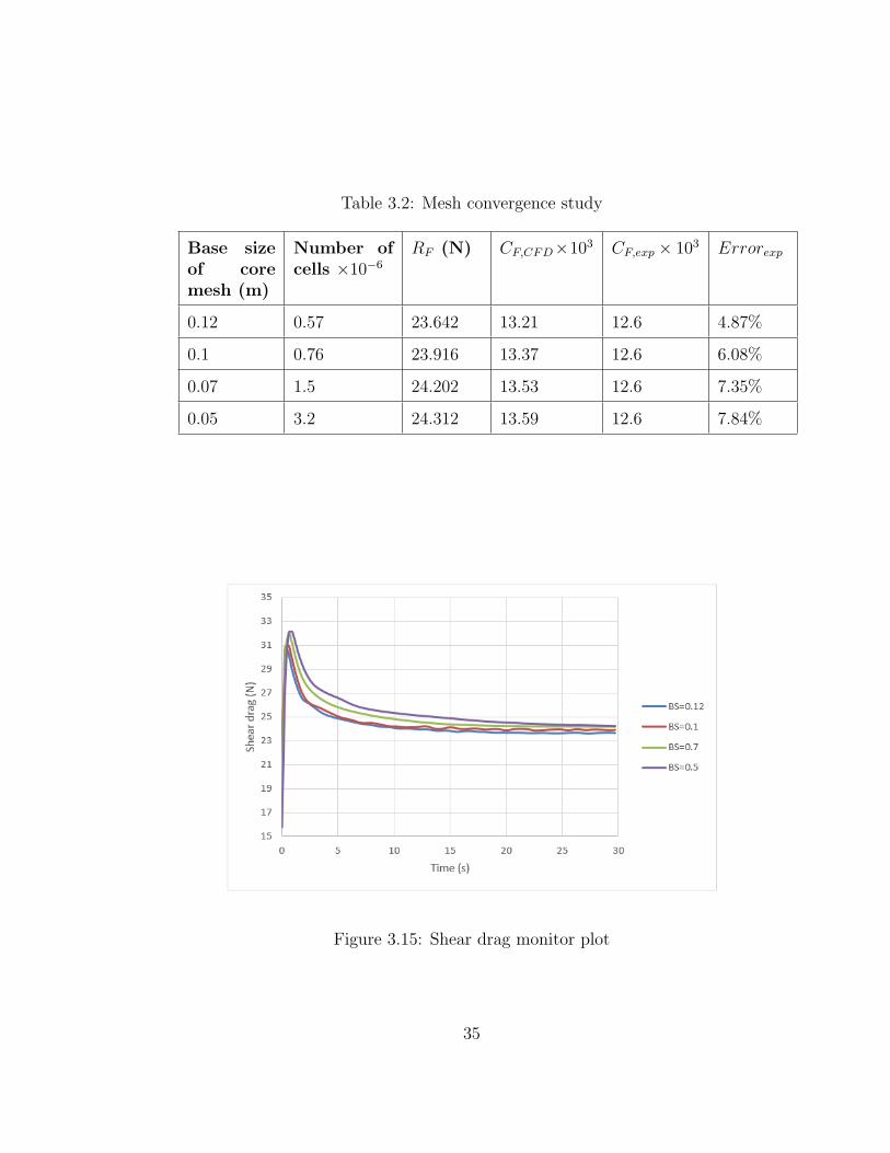
Table 3.2: Mesh convergence study
Base sizeof coremesh (m)
Number ofcells ×10−6
RF (N) CF,CFD×103 CF,exp × 103 Errorexp
0.12 0.57 23.642 13.21 12.6 4.87%
0.1 0.76 23.916 13.37 12.6 6.08%
0.07 1.5 24.202 13.53 12.6 7.35%
0.05 3.2 24.312 13.59 12.6 7.84%
Figure 3.15: Shear drag monitor plot
35

Figure 3.16: Shear drag in the last 12 seconds
Figure 3.17: Improper mesh transition (base size=0.05m)
36

Figure 3.18: Improper mesh topology (base size=0.12m)
3.2.2 Time step
After an initial wall convergence study, the time step was changed to assess
its effect on convergence (Table 3.3). It is seen that reducing the time brings
about faster convergence from the simulated physical time standpoint (Figure
3.19). However, the smaller the time step, the greater the computational time.
Considering these facts, and noting that the best results were obtained with a
time step of 0.3 second, it was decided to select a time step of 0.3 second to
proceed further in the study.
3.2.3 Wall treatment
The result of a simulation analyzing surface roughness is very sensitive to the
wall treatment, especially at high roughness levels. STAR CCM+ offers three
wall treatment models. The low-Y + model resolves the viscous sublayer and
37

Table 3.3: Time convergence study
Time step(s)
Number ofcells ×10−6
RF (N) CF,CFD×103 CF,exp × 103 Errorexp
0.1 0.78 22.838 12.76 12.6 1.25%
0.3 0.78 22.781 12.73 12.6 1.05%
0.5 0.78 22.883 12.78 12.6 1.5%
0.7 0.78 23.037 12.87 12.6 2.18%
Figure 3.19: Time convergence plot
is computationally expensive; the high-Y + model does not resolve the viscous
sublayer but uses wall functions to derive flow variables; the all-Y + model is a
hybrid wall treatment suitable when it is difficult to achieve a pure low-Y + or
a pure high-Y + (CD-ADAPCO, 2017).
An all-Y + wall treatment has been selected for this study. When using this
model, it is recommended that the initial wall cell centroid falls within the
buffer layer (Figure 3.20). The sensitivity of the simulation results for fouled or
38

unfouled plates to the initial wall cell size can be seen in Tables 3.4 and 3.5. In
any case, it appeared from the analysis of several other simulations that the best
configuration is obtained when the initial wall cell size y0 is comprised between
8% and 15% of an estimate of the boundary layer thickness δlim at half-length:
0.08δlim < y0 < 0.15δlim (3.11)
δlim = 5.926L
2· CF,r (3.12)
Here, L is the length of the plate or ship, and CF,r is an estimated fully-rough
frictional resistance coefficient at L2
given as (Faltinsen, 2005):
CF,r = [1.89 + 1.62 log(L
2ks)]−2.5 (3.13)
It is of note that this estimate of the boundary layer thickness assumes a fully-
rough flow regime (Section 3.1.6). Even though it is considered accurate enough
for this study, it is recommended to further investigate its validity.
The initial wall cell size can be adjusted by varying the number of prism layers
near the wall and their stretching.
Table 3.4: Initial wall cell size study (fouled Silicone 1)
y0δlim
(%) Number ofcells ×10−6
RF (N) CF,CFD×103 CF,exp × 103 Errorexp
2.2 0.88 14.314 7.999 12.6 −36.51%
6.8 0.82 20.913 11.688 12.6 −7.24%
11.3 0.78 23.41 13.086 12.6 3.86%
24.9 0.74 26.343 14.723 12.6 16.85%
39

Figure 3.20: Initial wall cell size requirement for each wall treatment model(CD-ADAPCO, 2017)
Table 3.5: Initial wall cell size study (unfouled Silicone 1)
y0δlim
(%) Number ofcells ×10−6
RF (N) CF,CFD×103 CF,exp × 103 Errorexp
7.9 0.9 6.281 3.511 3.666 −4.24%
14.6 0.86 6.499 3.632 3.666 −0.92%
25.4 0.8 6.641 3.711 3.666 1.25%
35.3 0.78 6.654 3.719 3.666 1.45%
Note on the derivation of δlim
A turbulent boundary layer thickness at a distance x from the leading edge of
a plate can be approximated as:
δ =0.16x
(Rn,x)17
(3.14)
The local skin friction at the location x can also be approximated as (Faltinsen,
40

2005):
Cf,x =0.027
(Rn,x)17
(3.15)
Combining Equations 3.14 and 3.15, we have
δ = 5.926x · Cf,x (3.16)
By definition of the (total) frictional resistance coefficient CF , the following
relationship holds:
δ = 5.926x · Cf,x < 5.926x · CF (3.17)
Which leads us to an upper estimate of the boundary layer thickness δlim at
half-length of the plate - or ship - given in Equation 3.12.
3.3 Validation Study
The results of the simulations were validated against the experimental data
published by Schultz (2004). Table 3.6 shows that there is excellent agreement
between the simulations and the real experiment with the error in all cases not
exceeding ±4%.
3.4 Results/Prediction
A prediction study was made for the frigate hull form described in Table B.1
and Figure 3.21. The mesh and time step of the simulations were set up with the
Estimated Hull Performance add-on of Star CCM+, producing meshes similar
to the validation study (note the volumetric refinements in Figures 3.23 and
41

Table 3.6: Comparison of experimental (Schultz, 2004) vs simulated CF atRn = 2.8 · 106
RF (N) CF,CFD×103
CF,exp×103
Errorexp
Unfouled
Smooth 6.329 3.537 3.605 −1.87%
Silicone 1 6.499 3.632 3.666 −0.92%
Silicone 2 6.533 3.651 3.663 −0.32%
Ablative Copper 6.517 3.643 3.701 −1.58%
SPC Copper 6.541 3.656 3.736 −2.14%
SPC TBT 6.614 3.697 3.776 −2.10%
Fouled Silicone 1 23.41 13.086 12.6 3.86%
Silicone 2 24.96 13.948 13.7 1.81%
Ablative Copper 12.49 6.978 6.770 3.07%
SPC Copper 14.57 8.140 8.010 1.63%
SPC TBT 10.20 5.699 5.720 −0.37%
3.24). The physics and wall treatment were set up identical to the validation
study.
The analysis has been restricted to fouling conditions below FR-60 (small cal-
careous fouling) since ships are rarely let fouled beyond this condition. The
detrimental effect of fouling can be seen in Figures 3.25 and 3.26. As expected,
the following observations can be made:
• The rougher the surface, the greater the increase in frictional resistance;
• The frictional resistance increases with speeds for a given roughness con-
dition;
• The frictional resistance doubles at 30 kts for the small calcareous fouling
42

condition;
• The relative increase in total resistance decreases at high speeds due to
the sharp increase in the contribution of wave resistance at Fn ≈ 0.3.
It is of note that the results obtained here are close to the predictions of Schultz
(2007) for a FFG-7 frigate (120 m long).
Figure 3.21: Hull form of a frigate (MAXSURF)
Figure 3.22: Domain view for the prediction study
43

Figure 3.23: Overall mesh for the prediction study
(a) Front view (b) Side view
(c) Top view
Figure 3.24: Frigate mesh
44

(a) RF against velocity (b) RT against velocity
(c) % Increase of RF (d) % Increase of RT
Figure 3.25: Variation of resistance with speed and fouling condition
45

(a) CF against Froude number (b) CT against Froude number
(c) % Increase of CF (d) % Increase of CT
Figure 3.26: Variation of resistance coefficients with speed and fouling condition
46

Chapter 4
MATLAB Code
This section presents the procedure implemented in a MATLAB code to find the
additional engine power needed to overcome fouling at a given speed. Then, the
calculated rough frictional resistance coefficient, which is key to estimating the
hydrodynamic penalty of biofouling, is compared against experimental results.
Finally, the procedure to determine the best time to clean a hull has been
presented. An analysis of the penalty for various ship types has also been
discussed.
4.1 Procedure to Find Added Power Due to
Fouling
The procedure to find the required propulsive power of a ship can be adapted to
find the extra power required when the hull is fouled. The assumptions are the
same, i.e. the frictional resistance is a function of the wetted surface and the
speed. The fouling condition needs to be considered since it affects the frictional
47

resistance through the roughness function.
Consequently, the inputs of the code are:
• the roughness height k based on Equations 2.14a, 2.14b, 2.14c or Table
2.3,
• the velocity of the ship U (this could be a range in vector form),
• the length of the ship L, and
• the wetted surface area of the ship S.
From these inputs, the added power due to fouling to keep the ship sailing at
U is calculated as follows:
(e) the Reynolds number of the ship Rn = U ·Lν
;
(f) The corresponding CF,r is found using steps (b) to (d) as described in the
similarity scaling procedure (section 2.4). Step (a) is omitted since the
roughness function is defined by Equation 2.14;
(g) CF,clean for a clean coating is found using kclean from Equation 2.14a or
Table 2.3;
(h) ∆CF = CF,r − CF,clean;
(i) ∆PE = 12ρ ·∆CF · S · U3;
(j) ∆PB = ∆PEη
.
48

4.2 Calibration and Validation of the Code
As already mentioned, application of Granville similarity scaling law requires
the definition of ∆U+ or reference points. Here, the reference points are chosen
from the towing tank experiments of Schultz (2004).
Firstly, an appropriate smooth friction line had to be adopted. It is seen in
Figure 4.1 that the Schoenherr friction line (Equation 2.6) correlates more to the
measurements than the ITTC-1957 friction line (Equation 2.7). This is in line
with the recommendation of Schultz (2004) and is consistent with the idea that
the ITTC formula is a model-ship correlation line. Therefore, the Schoenherr
friction line was adopted for all predictions. Note that further comparison of
the predictions with both friction lines confirmed this choice as the best.
Figure 4.1: Comparison of ITTC, Schoenherr friction lines and experimentalCF (experimental data from Schultz (2004))
Secondly, the predictions were made for L1 = L2 = 1.52m in order to ensure
that when no offset of length is made (log (L2
L1) = 0), the reference points are
49

obtained.
For all predictions of unfouled coatings, the margin of error between predicted
and measured frictional coefficients CF is ±2% (Figure 4.2). For the predictions
of barnacle-fouled surfaces, it was found that using k as defined in Equation
2.14c yielded errors of up to 13% in frictional resistance coefficient. For this
reason, the roughness length scale was modified as shown in Equation 4.1 which
yielded better results:
k = 0.042Rt
√%Barnaclefouling (4.1)
The calculated error in this case was ±3%. For the surface covered with slime
only, the predicted CF had a maximum error of 6%. No attempt was made to
change Equation 2.14b due to the lack of experimental data on slime-only cov-
ered surfaces. Figure 4.2 shows the excellent agreement between the predicted
and the measured values of CF .
It is interesting to note that the modified roughness length scale (Equation
4.1) agreed well with the classic pontoon experiment of Kempf (1937) where he
conducted experiments at the Hamburg Model Basin (HSVA) tank to assess the
impact of macrofouling on the resistance of ships (Figure 4.3). The maximum
noted error in CF is ±4% when using Equation 4.1. However, it rises to 9%
when using Equation 2.14c.
At this point, it is relevant to note that there is excellent agreement between the
predictions of the code which, as a reminder, is based on turbulent flow similarity
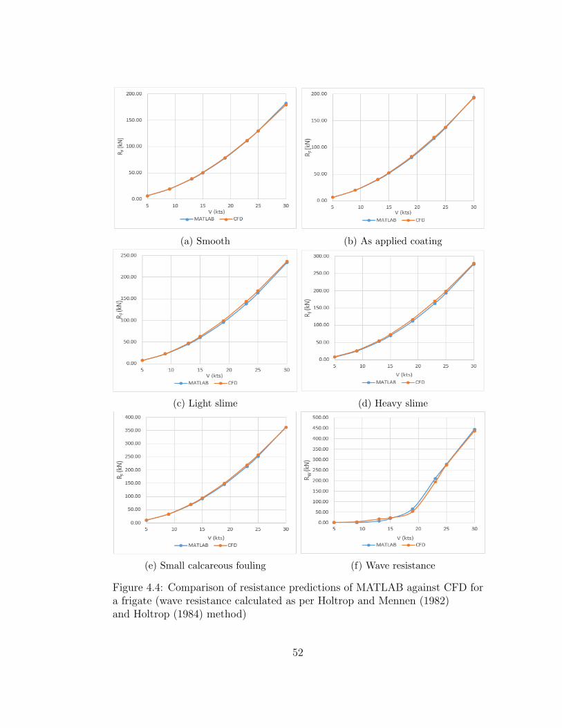
scaling (Section 2.4), and the CFD predictions as evidenced by Figure 4.4.
50

Figure 4.2: Comparison of experimental and calculated CF (experimental datafrom Schultz (2004))
Figure 4.3: Comparison of experimental and calculated CF (experimental datafrom Kempf (1937))
51
(a) Smooth (b) As applied coating
(c) Light slime (d) Heavy slime
(e) Small calcareous fouling (f) Wave resistance
Figure 4.4: Comparison of resistance predictions of MATLAB against CFD fora frigate (wave resistance calculated as per Holtrop and Mennen (1982)and Holtrop (1984) method)
52

4.3 Biofouling Tolerability Prediction
4.3.1 Method
If the added power due to fouling is known for a ship having a specific operational
profile and a specific coating system, the best time to clean a sister ship under
the same conditions (or the same ship during her next period of activity) can
be inferred.
Firstly, the roughness height for the entire hull after a given period of activity
must be assessed. Hulls of ships are almost never covered with uniform fouling.
For example, the uneven distribution of light or the difference in flow character-
istics along the hull affects fouling species distribution (INTERTANKO, 2016;
Swain and Lund, 2016). However, when analyzing the roughness of a hull, it is
possible to subdivide the hull in m zones, visually assess the fouling condition of
each zone, and determine a weighted average roughness height for the entire hull
as k =m∑j=1
(%area)j · kj100
, where (%area)j and kj are respectively the percent
relative area and the roughness height of each zone.
Secondly, the added power due to fouling is determined using the procedure
described in section 4.1. To achieve this, the type of function that governs the
increase of fouling over time has to be assumed from observation (linear, ascen-
dant sinusoid, square-root, etc.). For example, Aertssen (1966) observed that
the added power due to fouling on MV Jordaens followed nearly a square-root
curve, which suggests a linear roughness increase over time; after several sea
trials in temperate waters, Lewthwaite et al. (1985) observed that the increase
in local skin friction Cf due to slime followed an ascendant sinusoid (seasonality
effect), which suggests likewise for the roughness increase over time; or a piece-
53

wise linear function could be adopted to account for an accelerated growth of
fouling in ports. It is expected that the governing function would be dependent
upon the coating system and the operational profile of the vessel (geographic
area of operation, time at berth, speed, etc.).
Finally, the time T at which the cumulative cost of fouling overcomes the clean-
ing cost is determined using the following steps:
(k) The function k(t) is defined based on the time spent at sea Tsea, and dis-
cretized with n+ 1 data points ki = k(ti), i = 0, . . . , n;
(l) ∆PB(ti) = f(ki) is calculated using steps (e) to (j) described above (section
4.1);
(m) The sum of all added power due to fouling over time is KF (t) =∫
∆PBdt,
which by trapezoidal rule of integration can be approximated as KF =n∑i=1
(ti − ti−1)∆PB(ti−1) + ∆PB(ti)
2;
(n) The cumulative extra fuel consumption over time is FC(t) = SFOC ·KF (t),
where SFOC is the specific fuel oil consumption of the engine;
(o) The cumulative cost of extra fuel burned over time is Cfuel(t) = cfuel ·FC(t),
where cfuel is the fuel price;
(p) Finally, T is the solution of the equation: Cfuel(t) = Cc, where Cc is the
cleaning cost (equivalently, T is determined by the intersection of the curve
of added fuel cost and the cleaning cost line).
A summary of the procedure is presented in Figure 4.5.
54

Figure 4.5: Summary of the biofouling tolerability prediction method for ships
55

4.3.2 Results
Prediction Study for a Cruise Ship
Let us consider a hypothetical scenario - the assumptions are summarized in
Table 4.1 - involving a Cruise ship (Figure 4.6). After one year at sea without
underwater cleaning, her fouling condition is described in Table 4.2 and Figure
4.7 (based on observations by Koka (2014)).
Figure 4.6: Cruise ship model (MAXSURF)
With the assumption that fouling rate follows a linear increase, we have k(t) =
a·t+kclean, where t denotes time in hours, and kclean is determined from Equation
2.14a.
We know k(8760) = 40.4µm, so k(t) = 0.004t+ 5.1 [µm].
By discretizing n = 100, the resultant added power and added fuel cost over
time are calculated using steps (k) to (p) and plotted in Figure 4.8. It shows
that the extra fuel cost exceeds the cleaning cost after nearly 40 days or 1000
hours when the ship is sailing at the cruising speed of 20 knots. If an average
operational ship speed of 15 knots is assumed, the threshold is overcome after
nearly 60 days at sea or 1500 hours of operation. As expected, higher speeds
mean more detrimental effect of fouling.
56

Table 4.1: Summary of assumptions for the Cruise ship prediction
Ship L = 314m
S = 13347m2
U = 20kts
SFOC = 0.171 kg/kWh
η = 0.75
Ra = 30µm (applied fouling release coating)
Fouling condi-tion
In-dock observations: refer Table 4.2
Fouling rate: follows a linear increase
Time at sea before docking: 1 year (8760 hours)
Market Fuel price (IFO 380)=$370/tonne (Source: Ship andBunker, 2017)
Cleaning cost=$20, 000 per occurrence
Table 4.2: Fouling condition
Zone % area relativeto total area
Condition Roughness height(Table 2.3)
1 17 Light biofilm k1 = 17µm
2 74 Light to moderatebiofilm
k2 = 23.5µm
3 3 Moderate biofilm and /or green weed
k3 = 30µm
4 6 Heavy green weed k4 = 320µm
Weighted average roughness height k = 40.4µm
57

Figure 4.7: Percent distribution of fouling on fouling release coating observedon 5 cruise ships (Koka, 2014)
Figure 4.8: Added power and cumulative extra fuel cost for a cruise ship
58

The adverse effect of speed for a given fouling condition can be further evaluated
in Figure 4.9. Under the earlier assumptions (k ≈ 40µm), the added cost of
fuel due to fouling in a single day at a speed of 25 knots is over half that
of the cleaning cost, i.e the cleaning cost would be overcome in two days of
operations. If the propulsive power is set to a constant value however, there
will be an induced reduction in speed which can be quite significant.
Figure 4.9: Added daily fuel consumption and costs for a cruise ship
Prediction of Biofouling Tolerability for Various Ship Types
In this section, the tolerability of fouling for different ship types is analyzed.
Three MAXSURF model bare hull forms have been selected representing re-
spectively a Cruise ship, a Frigate and a Trawler (Figures 4.10 to 4.12). The
main particulars of each hull are listed in Table 4.3, and the assumptions for the
tolerability prediction are the same as in Table 4.1. The cleaning costs ranges
59

are typical values given by ABS (2013) and McMillan and Jarabo (2013).
Table 4.3: Ship particulars
Cruise ship Frigate Trawler
LWL(m) 314.412 80.000 24.028
B(m) 38.595 12.521 5.640
T (m) 8.800 3.000 1.500
∆(t) 67396 1378 114.5
CB 0.616 0.447 0.550
CM 0.901 0.827 0.858
S(m2) 12985.395 924.926 144.950
Figure 4.10: Hull form of a cruise ship (MAXSURF)
Figure 4.11: Hull form of a frigate (MAXSURF)
60

Figure 4.12: Hull form of a trawler (MAXSURF)
Figure 4.13: Fouling tolerability analysis for a cruise ship
61

Figure 4.14: Fouling tolerability analysis for a frigate
Figure 4.15: Fouling tolerability analysis for a trawler
62

4.4 Percent Fouling Penalty Calculation
4.4.1 Method
In this section, the fouling penalty is analyzed with respect to the total power
requirement. Indeed, it is often convenient to analyze the hydrodynamic impact
of biofouling in terms of percentage, especially to facilitate comparisons among
different ships. Though noted %(∆PE), it should be borne in mind that the
percent penalty is the same whatever the standpoint in the propulsion line i.e.:
%(∆PB) =PB,r − PB,s
PB,s· 100 =
ηPB,r − ηPB,sηPB,s
· 100 =PE,r − PE,s
PE,s· 100
%(∆PB) = %(∆PE)
(4.2)
Now combining with Equation 2.8, we have
%(∆PE) =RT,r · U −RT,s · U
RT,s · U· 100
%(∆PE) =12ρ(CT,s + ∆CF )SU3 − 1
2ρCT,sSU
3
12ρCT,sSU3
· 100
(4.3)
In other words,
%(∆PE) =∆CFCT,s
· 100 (4.4)
Considering that wave resistance is the major component of the residuary re-
sistance, we shall derive from ITTC-1978 that
CT,s = (1 + k1)CF + CR + CA ≈ (1 + k1)CF + CW + CA (4.5)
63

Rewriting Equation 4.4,
%(∆PE) =∆CF
(1 + k1)CF + CW + CA· 100 (4.6)
The MATLAB code makes use of Holtrop (1984) and Holtrop and Mennen
(1982) formulations for form factor, wave resistance and correlation allowance
(respectively Equations A.18, A.4 and A.19) to assess the percent penalty.
4.4.2 Variability/Similarity of Fouling Penalty with Ship
Types
In this section, the variability of the percent fouling penalty with ship types is
analyzed. It seems that there is in fact some similarity among ship types when
they are scaled with respect to their Froude number.
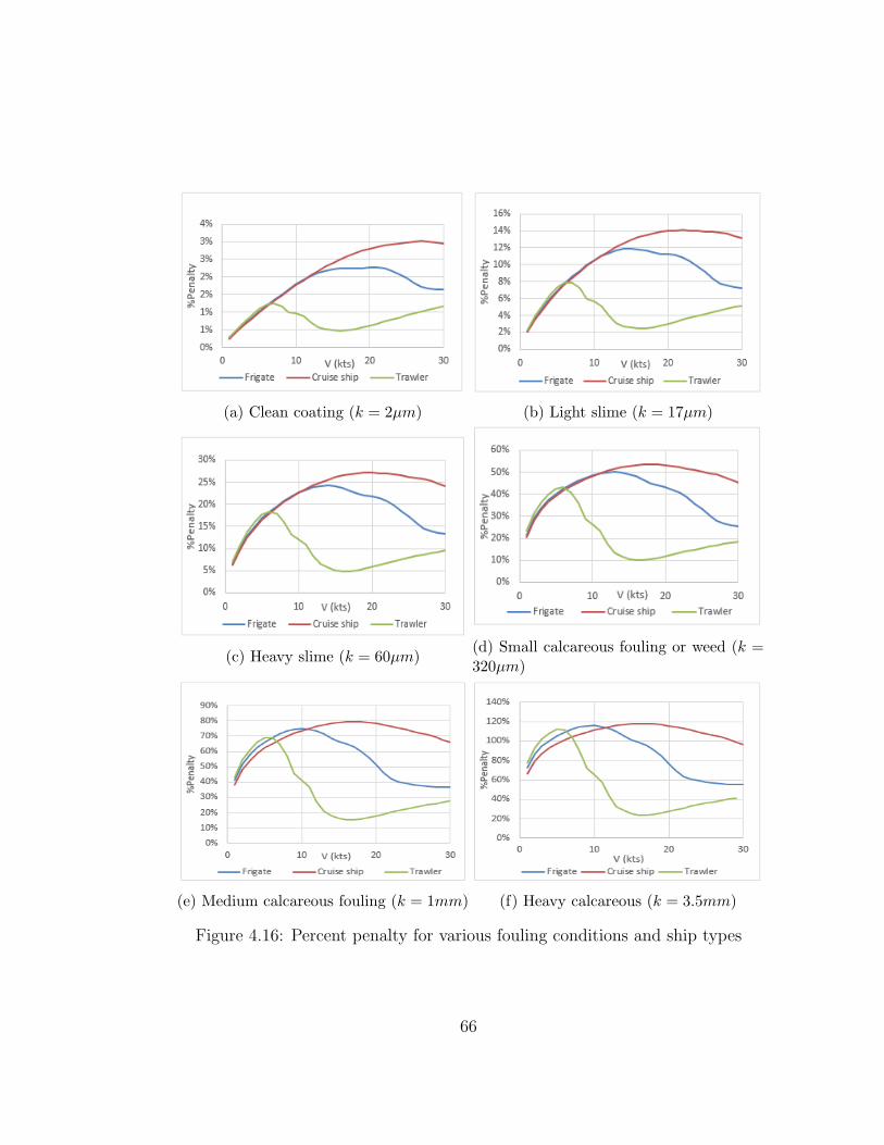
The percent penalty for all three ship types are plotted against velocity in
Figure 4.16. Interestingly, when plotted against Fn, the percent penalty of two
different ships seems strongly correlated (especially at Fn less than 0.3) as shown
in Figures 4.17 and 4.18. From this study, the correlation has been found to be:
%(∆PE)1 = %(∆PE)2 · (1 + α log
(Rn,1
Rn,2
)) · (1 + k1)2
(1 + k1)1
(4.7)
Where α = 2.25e−3.74√k.
Equation 4.7 has been found by noting the following:
• The percent penalty as given by Equation 4.6 is a function of CW , CF
and ∆CF , hence also a function of Fn, Rn and k (roughness height) -
neglecting the effects of CA;
64

• The gap in percent penalty plotted against Fn for the various ship types
is inversely proportional to the roughness height k (Figure 4.17).
At the same velocity, Equation 4.7 can be rewritten as:
%(∆PE)1 = %(∆PE)2 · (1 + α log
(L1
L2
)) · (1 + k1)2
(1 + k1)1
(4.8)
If the form factors are neglected, the relationship is simplified as follows:
%(∆PE)1 = %(∆PE)2 · (1 + α log
(L1
L2
)) (4.9)
65
(a) Clean coating (k = 2µm) (b) Light slime (k = 17µm)
(c) Heavy slime (k = 60µm)(d) Small calcareous fouling or weed (k =320µm)
(e) Medium calcareous fouling (k = 1mm) (f) Heavy calcareous (k = 3.5mm)
Figure 4.16: Percent penalty for various fouling conditions and ship types
66

(a) Clean coating (k = 2µm) (b) Light slime (k = 17µm)
(c) Heavy slime (k = 60µm)(d) Small calcareous fouling or weed (k =320µm)
(e) Medium calcareous fouling (k = 1mm) (f) Heavy calcareous (k = 3.5mm)
Figure 4.17: Percent penalty vs Fn for various fouling conditions and ship types
67

(a) Clean coating (k = 2µm) (b) Light slime (k = 17µm)
(c) Heavy slime (k = 60µm)(d) Small calcareous fouling or weed (k =320µm)
(e) Medium calcareous fouling (k = 1mm) (f) Heavy calcareous (k = 3.5mm)
Figure 4.18: Scaled percent penalty vs Fn for various fouling conditions andship types
68
4.5 Discussion
An effective numerical modelling of biofouling has the potential to improve cur-
rent biofouling management practices. Two applications of such attempt with
a MATLAB code have been presented that respectively assess the tolerability
of biofouling and its hydrodynamic penalty.
The first application shows that it is possible to evaluate when biofouling is no
longer tolerable in a given context considering its cumulative economic penalty.
This information would be useful in a bigger maintenance strategy to comple-
ment other fouling management tools since none of them is perfect. Antifouling
coating systems cannot achieve 100% immunity; monitoring hull performance
is prone to error due to the influence of weather, loading condition, currents,
etc. (Munk et al., 2009; Townsin, 2003); hull cleaning is unproductive if it does
not occur at a proper timing.
Today, it is very common to determine when hull cleaning should occur by mon-
itoring hull performance or visual observation. However, this reactive approach
may not be suitable in all circumstances. The prediction of fouling tolerability
fits well into a proactive fouling management strategy that some studies ad-
vocated (Tribou and Swain, 2010). A proactive approach allows for effective
planning. For example, hull cleaning may take one or two days and ship inac-
tivity may be inconvenient if not planned ahead of time. It further helps ship
operators ensure that the money spent into fouling precautions is optimally in-
vested. A coating system, for instance, will be selected based upon its resistance
to fouling against its ability to sustain multiple cleaning. Recoating costs may
also be put into balance.
An interesting aspect of the current numerical code is its flexibility as it en-
69
deavors to account for the specifics of each case. For example, fouling rate is
determined based on at least one observation of the fouling condition of the ship
considered. If such an observation is made at the end of an operational cycle -
and in between, if many observations are possible - an appropriate knowledge of
the marine growth can be inferred. The fouling rate governing function can also
be adapted to consider the duration of the ship at berth. Moreover, the increase
in resistance for a given fouling condition is dependent on vessel type and speed
which, in the proposed method, are considered as input. As demonstrated by
the analysis of three different ship types, a universal drag factor does not reflect
the specifics of each case.
The second application uses empirical formulations of the wave resistance of
ships to assess the percent penalty incurred by biofouling. This traditional way
of expressing the penalty is useful to compare the vulnerability of different ships
to fouling. The analysis shows that for the same fouling condition and speed,
bigger ships have a greater penalty. This is not surprising as the contribution of
frictional resistance is proportional to the wetted surface area. One would tend
to clean bigger ships more often than smaller ones. However, since cleaning
costs are relatively smaller for bigger ships, it is best to heed the tolerability
prediction method in order to make thoughtful decisions.
It is also interesting to note the correlation of the penalty among ship types.
It is seen that a good approximation of the fouling penalty for any ship can be
obtained from Equation 4.7. Certainly, this correlation needs further investiga-
tion.
70

Chapter 5
Conclusion
The present work has shown the implementation of two numerical methods to
assess the impact of biofouling on the hydrodynamics of ships. Both methods
are validated against experimental data available in the literature.
The first method is a CFD assessment of the additional drag incurred by bio-
fouling. The merit of this approach lies in the use of a fully-defined ship model
to simulate the hydrodynamic impact of fouling. It has the potential to reduce
the need for costly experiments on ships. If appendages and superstructure
are modelled, an accurate prediction of the residuary resistance can be made,
leading also to an accurate prediction of the percent penalty. The validity of
the model presented could be further investigated and compared against exper-
imental results.
The second method developed in MATLAB is a flexible, much faster instrument
that could be used to predict when the penalty due to biofouling on a ship
overcomes the cleaning cost. The tool aims to account for the specifics of each
situation through at least one observation of the fouling condition of a given ship.
71

A direct measure of the economic penalty in dollar amount is given as well as a
relative measure in percentage. With further improvements, the code might be
able to estimate the penalty from a pictorial representation of a fouled hull. This
would certainly ease in-dock assessments and improve proactive management of
ship operations.
It goes without saying that the reliability of the methods herein presented is tied
to the reliability of the mathematical models used. Several studies have pointed
out the complexity of characterizing and modelling marine fouling, especially
biofilms. In particular, Table 2.3 and equation 2.14 need much supportive work.
In the end, if it is true that the present work presents two distinct methods that
can serve as good approximation tools, research still needs to be done for more
accurate predictions.
72

Chapter 6
Recommendations for future
research
The study presented in this thesis is an attempt to model biofouling and estimate
its penalty. Both numerical methods discussed could be further improved. It is
also possible to push the analysis further into areas not explored here.
The CFD analysis has been limited by the time and the computational resources
available. The precision of the predictions could be improved by creating finer
meshes. With that said, finer meshes will only produce meaningful results if
the transition from prism layer cells to core mesh cells is smooth, and if the
simulations are run for enough time to achieve convergence. From the author’s
point of view, no less than 1.5 million cells should be used.
Another area of improvement in CFD is the wall treatment. From the author’s
analysis, the first cell size has to relate to the boundary layer thickness. An
alternative equation to Equation 3.12 could be used to assess the boundary
layer thickness. Other recent studies have reported that y+ should be greater
73

than k+ for accurate results (Demirel et al., 2017). This statement could also
be further investigated.
Areas not explored in this study that are worthy of interest are the use of CFD
to assess the effectiveness of partial hull cleaning. Through the input of various
roughness heights along the hull, it is possible to analyze the benefit of having
some portions of the hull cleaned instead of others (bow, shoulder, stern, etc.).
Also, it is necessary to ascertain the mathematical formulations used (roughness
function, fouling reference table) through experiments. In particular, biofilms
could be analyzed as viscoelastic fluids instead of solid bodies (sand roughness).
The code implemented in MATLAB, which is also available as a MATLAB
application, could be refined to incorporate more parameters. Such a flexible
tool, as demonstrated by its use in the tolerability prediction method, is capable
of producing prompt results. From the author’s point of view, it holds a lot of
potential. However, it definitely needs experts’ advice to produce useful and
more realistic results.
74

References
ABS (2013). Ship energy efficiency measures.
Aertssen, G. (1966). Service performance and seakeeping trials on MV Jordaens.
In Trans. RINA, volume 105, pages 293–335.
CD-ADAPCO (2017). STAR-CCM+ User guide.
Cebeci, T. and Bradshaw, P. (1977). Momentum transfer in boundary lay-
ers. In Momentum transfer in boundary layers, pages 176–180. Hemisphere
Publishing/McGraw-Hill.
Cebeci, T., Shao, J. P., Kafyeke, F., and Laurendeau, E. (2005). Computational
fluid dynamics for engineers: from panel to Navier-Stokes methods with com-
puter programs. Horizons Pub. Inc., ; Springer, Long Beach, Calif. : Berlin.
Cengel, Y. A. and Cimbala, J. M. (2006). Fluid mechanics: fundamentals
and applications. McGraw-Hill series in mechanical engineering. McGraw-
HillHigher Education, Boston.
Demirel, Y. K., Khorasanchi, M., Turan, O., Incecik, A., and Schultz, M. P.
(2014). A CFD model for the frictional resistance prediction of antifouling
coatings. Ocean Engineering, 89:21–31.
75
Demirel, Y. K., Turan, O., and Incecik, A. (2017). Predicting the effect of
biofouling on ship resistance using CFD. Applied Ocean Research, 62:100–
118.
Faltinsen, O. M. (2005). Hydrodynamics of high-speed marine vehicles. Cam-
bridge university press.
Granville, P. S. (1958). The frictional resistance and turbulent boundary layer
of rough surfaces. Journal of Ship Research, 2:52–74.
Haslbeck, E. G. and Bohlander, G. S. (1992). Microbial biofilm effects on drag-
lab and field. Technical report, DTIC Document.
Holtrop, J. (1984). A statistical re-analysis of resistance and propulsion data.
International Shipbuilding Progress, 31:272–276.
Holtrop, J. and Mennen, G. G. J. (1982). An approximate power prediction
method. International Shipbuilding Progress, 29(335):166–170.
Hunsucker, J. T., Hunsucker, K. Z., Gardner, H., and Swain, G. (2016). Influ-
ence of hydrodynamic stress on the frictional drag of biofouling communities.
Biofouling, 32(10):1209–1221.
Hunsucker, K. Z., Koka, A., Lund, G., and Swain, G. (2014). Diatom community
structure on in-service cruise ship hulls. Singapore.
IMO (2011). Guidelines for the control and management of ships’ biofouling to
minimize the transfer of invasive aquatic species.
INTERTANKO (2016). INTERTANKO guide to modern antifouling systems
and biofouling management.
76

IPPIC (2010). Prevention of air pollution from ships. Technical Report MEPC
60/4/21, International Maritime Organisation.
Kattan, M. R., Townsin, R. L., and Armstrong, V. N. (2015). Managing the
underwater hull. SNAME Symposia papers.
Kempf, G. (1937). On the effect of roughness on the resistance of ships. In
Trans. INA, volume 79, pages 109–119.
Koka, A. K. (2014). A methodology for the inspection of antifouling coatings
during ship dry docking. Master of Science, Florida Institute of Technology,
Melbourne.
Lewthwaite, J. C., Molland, A. F., and Thomas, K. W. (1985). An investigation
into the variation of ship skin frictional resistance with fouling. In Trans.
RINA, volume 127, pages 269–284. The Royal Institution of Naval Architects.
McMillan, C. and Jarabo, A., editors (2013). Ship efficiency: the guide: a
comprehensive guide to ship eco-efficiency technologies and measures. Fathom
Shipping, Windsor, 2nd. ed edition.
Molland, A. F., Turnock, S. R., and Hudson, D. A. (2011). Ship resistance
and propulsion: practical estimation of ship propulsive power. Cambridge
University Press, New York.
Monty, J. P., Dogan, E., Hanson, R., Scardino, A. J., Ganapathisubramani, B.,
and Hutchins, N. (2016). An assessment of the ship drag penalty arising from
light calcareous tubeworm fouling. Biofouling, 32(4):451–464.
77

Munk, T., Kane, D., and Yebra, D. M. (2009). The effects of corrosion and
fouling on the performance of ocean going vessels: a naval architectural per-
spective. Advances in marine fouling technologies, pages 149–176.
Nikuradse, J. (1933). Laws of flow in rough pipes.
NSTM (2006). Waterborne underwater hull cleaning of Navy ships.
Oosterveld, M. (1978). Proceedings: 15th International Towing Tank Conference
: ITTC’78, The Hague, September 1978. Netherlands Ship Model Basin.
Schlichting, H. (1968). Boundary-layer theory. McGraw-Hill, New York, 6th
edition edition. OCLC: 923454798.
Schultz, M. P. (2004). Frictional Resistance of Antifouling Coating Systems.
Journal of Fluids Engineering, 126(6):1039.
Schultz, M. P. (2007). Effects of coating roughness and biofouling on ship
resistance and powering. Biofouling, 23(5):331–341.
Schultz, M. P., Bendick, J. A., Holm, E. R., and Hertel, W. M. (2011). Economic
impact of biofouling on a naval surface ship. Biofouling, 27(1):87–98.
Schultz, M. P. and Swain, G. W. (2000). The influence of biofilms on skin
friction drag. Biofouling, 15(1-3):129–139.
Schultz, M. P., Walker, J. M., Steppe, C. N., and Flack, K. A. (2015). Impact
of diatomaceous biofilms on the frictional drag of fouling-release coatings.
Biofouling, 31(9-10):759–773.
78

Swain, G. and Lund, G. (2016). Dry-Dock Inspection Methods for Improved
Fouling Control Coating Performance. Journal of Ship Production and De-
sign, 32(3):186–193.
Townsin, R. L. (2003). The Ship Hull Fouling Penalty. Biofouling, 19(sup1):9–
15.
Tribou, M. and Swain, G. (2010). The use of proactive in-water grooming
to improve the performance of ship hull antifouling coatings. Biofouling,
26(1):47–56.
WHOI and USN (1952). Marine fouling and its prevention. United States Naval
Institute, Annapolis, MD.
Zargiel, K. A. and Swain, G. W. (2014). Static vs dynamic settlement and
adhesion of diatoms to ship hull coatings. Biofouling, 30(1):115–129.
79

Appendix A
Calculation of wave resistance
In this study, the wave resistance and the wave resistance coefficient were calcu-
lated as proposed by Holtrop and Mennen (1982) and Holtrop (1984) regression
equations as follows :
• Fn ≤ 0.4
RW = c1c2c5ρg∇em1F dn+m4 cos (λF−2n ) (A.1)
• Fn ≥ 0.55
RW = c17c2c5ρg∇em3F dn+m4 cos (λF−2n ) (A.2)
• 0.4 < Fn < 0.55
RW = RW (Fn=0.4) + (10Fn − 4)[RW (Fn=0.55) −RW (Fn=0.4)]
1.5(A.3)
And finally, CW is given as:
CW =RW
12ρSU2
(A.4)
80
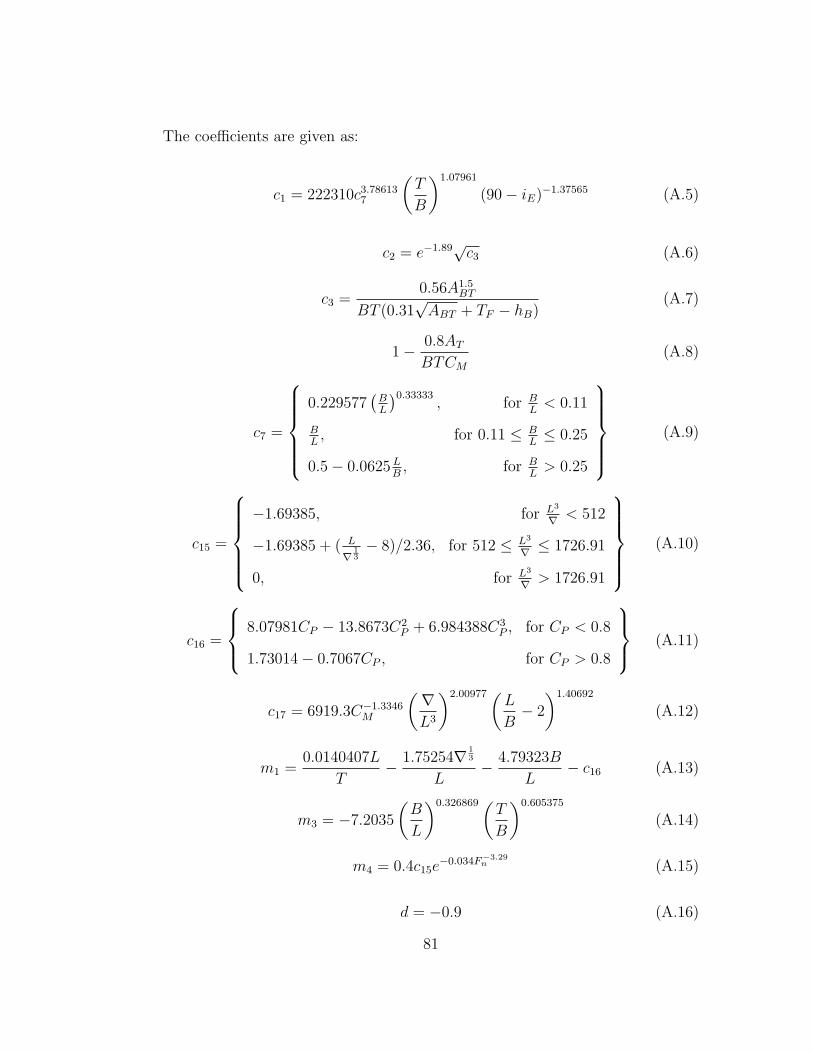
The coefficients are given as:
c1 = 222310c3.786137
(T
B
)1.07961
(90− iE)−1.37565 (A.5)
c2 = e−1.89√c3 (A.6)
c3 =0.56A1.5
BT
BT (0.31√ABT + TF − hB)
(A.7)
1− 0.8ATBTCM
(A.8)
c7 =
0.229577
(BL
)0.33333, for B
L< 0.11
BL, for 0.11 ≤ B
L≤ 0.25
0.5− 0.0625LB, for B
L> 0.25
(A.9)
c15 =
−1.69385, for L3
∇ < 512
−1.69385 + ( L
∇13− 8)/2.36, for 512 ≤ L3
∇ ≤ 1726.91
0, for L3
∇ > 1726.91
(A.10)
c16 =
8.07981CP − 13.8673C2P + 6.984388C3
P , for CP < 0.8
1.73014− 0.7067CP , for CP > 0.8
(A.11)
c17 = 6919.3C−1.3346M
(∇L3
)2.00977(L
B− 2
)1.40692
(A.12)
m1 =0.0140407L
T− 1.75254∇ 1
3
L− 4.79323B
L− c16 (A.13)
m3 = −7.2035
(B
L
)0.326869(T
B
)0.605375
(A.14)
m4 = 0.4c15e−0.034F−3.29
n (A.15)
d = −0.9 (A.16)
81

λ =
1.446CP − 0.03L/B, for LB< 12
1.446CP − 0.36, for LB> 12
(A.17)
The use of these expressions requires that the total resistance be calculated by
adopting the form factor concept (3D extrapolation procedure) which can be
calculated as follows:
1 + k1 = 0.93 + 0.487118c14
(B
L
)1.06806(T
L
)0.46106(L
LR
)0.121563
·(L3
∇
)0.36486
(1− CP )−0.604247
(A.18)
Where the length of run LR is defined as LR = L(1− CP + 0.06CP ·lcb4CP−1
).
The coefficient c14 accounts for the shape of the stern; assuming a normal stern
shape, c14 = 1.
The method also suggests formulations for the calculation of CA and the wetted
surface area S as follows:
CA = 0.006(L+ 100)−0.16 − 0.00205 + 0.003
√L
7.5C4Bc2(0.04− c4) (A.19)
Where c4 = T/L when T/L ≤ 0.04 or c4 = 0.04 otherwise.
S = L(2T +B)√CM(0.453 + 0.4425CB − 0.2862CM −
0.003467B
T
+0.3696CWP ) + 2.38ABTCB
(A.20)
82

Appendix B
Ship Particulars
Table B.1: Ship particulars
Cruise ship Frigate Trawler
LWL(m) 314.412 80.000 24.028
B(m) 38.595 12.521 5.640
T (m) 8.800 3.000 1.500
∇ (m3) 65956.907 1344.657 111.991
∆(t) 67396 1378 114.5
CB 0.616 0.447 0.550
CM 0.901 0.827 0.858
CP 0.687 0.551 0.633
CWP 0.802 0.718 0.858
S(m2) 12985.395 924.926 144.950
iE (deg) 9.9 7.9 26.3
AT (m2) 0 1.653 0.3
ABT (m2) 28.111 0 0.086
hB(m) 4.718 0 0
83
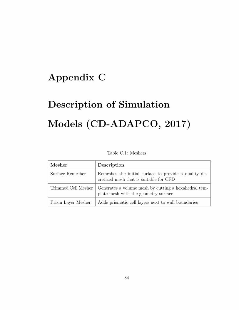
Appendix C
Description of Simulation
Models (CD-ADAPCO, 2017)
Table C.1: Meshers
Mesher Description
Surface Remesher Remeshes the initial surface to provide a quality dis-cretized mesh that is suitable for CFD
Trimmed Cell Mesher Generates a volume mesh by cutting a hexahedral tem-plate mesh with the geometry surface
Prism Layer Mesher Adds prismatic cell layers next to wall boundaries
84

Table C.2: Physical models
Model Description
All Y + wall treat-ment
Hybrid wall treatment using a blending approach suit-able for intermediate near-wall cell resolution
Cell Quality Remedi-ation
Improves the robustness of the solution by identifyingand remedying poor-quality cells
Eulerian Multiphase Defines the fluids involved in the flow (air, water)
Exact Wall Distance Makes an exact projection of the distance of cells nearthe wall to be used to account for near wall effects inno-slip boundary condition
Gradients Defines the method of gradients calculation for scalarvalues, flux, etc.
Gravity Accounts for the effects of gravitational acceleration
Implicit unsteady Controls the update at each physical time for the calcu-lation
K-Omega turbulence Provides closure of the RANS equations using K and ω
Multiphase Equationof State
Computes the density and density derivatives of eachfluid phase
Multiphase Interac-tion
Defines the action of one fluid phase upon another
Multiphase Mixture Considers mass, momentum and energy as mixturequantities
Segregated VolumeFlux Based Flow
Solves each of the momentum equations in turn
SST (Menter) K-Omega
Provides closure of the RANS equations with the SSTK − ω model
Three Dimensional Considers a 3-D geometry
VOF Waves Typically used for marine applications, it defines surfacegravity waves
Volume of Fluid(VOF)
Simulates flow of several immiscible fluids
85
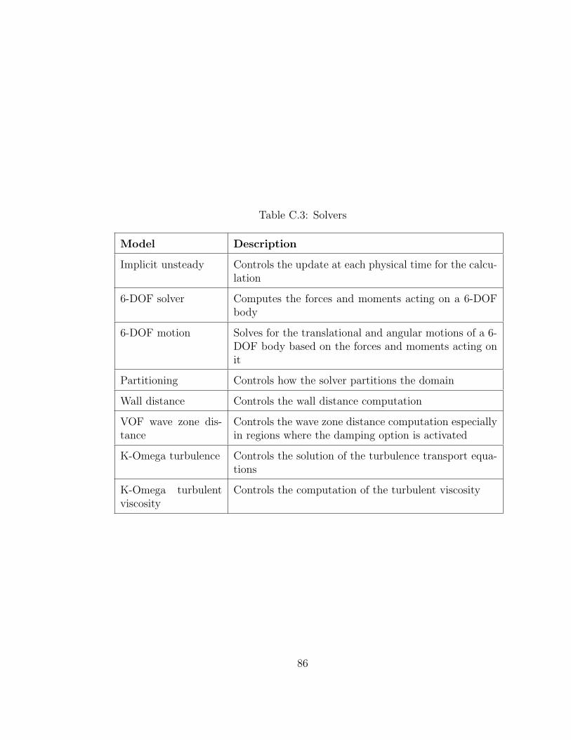
Table C.3: Solvers
Model Description
Implicit unsteady Controls the update at each physical time for the calcu-lation
6-DOF solver Computes the forces and moments acting on a 6-DOFbody
6-DOF motion Solves for the translational and angular motions of a 6-DOF body based on the forces and moments acting onit
Partitioning Controls how the solver partitions the domain
Wall distance Controls the wall distance computation
VOF wave zone dis-tance
Controls the wave zone distance computation especiallyin regions where the damping option is activated
K-Omega turbulence Controls the solution of the turbulence transport equa-tions
K-Omega turbulentviscosity
Controls the computation of the turbulent viscosity
86

Appendix D
CFD validation study
Herein, the details of the flow near the wall of the fouled Silicone 1 plate are
shown as an example. The friction velocity Uτ , the roughness Reynolds number
k+ and the normalized distance from the wall y+ are calculated as described in
section 2.3. Wall Y+ is calculated by STAR CCM+ as Wall Y+ = y0Uτν
where
y0 is the size of the initial wall cell.
Figure D.1: Wall shear stress τw over the plate (Pa = N/m2)
87

Figure D.2: Friction velocity Uτ over the plate
Figure D.3: Roughness Reynolds number k+ over the plate
88
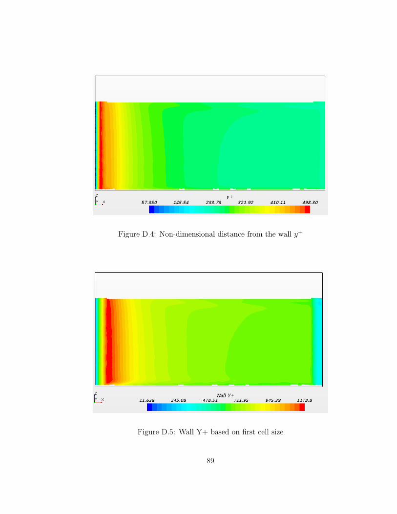
Figure D.4: Non-dimensional distance from the wall y+
Figure D.5: Wall Y+ based on first cell size
89