Embed Size (px)
Citation preview

Assessing Air Quality Impacts of
Managed Lanes
December 2010
Final Report
BDK85 TWO #977-11

II
ii
DISCLAIMER
The opinions, findings, and conclusions expressed in this publication are those of the authors and not necessarily those of the State of Florida Department of Transportation.

II
iii
Assessing Air Quality Impacts
of Managed Lanes
Final Report
Prepared for
State of Florida Department of Transportation
Public Transit Office
605 Suwannee Street, MS 30 Tallahassee, Florida 32399-0450
Project Manager: Amy Datz
Prepared by
Amy L. Stuart, Ph.D.
Pei-Sung Lin, Ph.D., P.E., PTOE
Changyoung Lee, Ph.D., PTP
Haofei Yu
Hongyun Chen
National Center for Transit Research
Center for Urban Transportation Research (CUTR) University of South Florida
4202 East Fowler Avenue, CUT100 Tampa, Florida 33620-5375
December 2010
BDK85 TWO #977-11

II
iv
1. Report No.
FDOT-BDK85-TWO #977-11 2. Government Accession No.
3. Recipient's Catalog No.
4. Title and Subtitle
Assessing Air Quality Impacts of Managed Lanes 5. Report Date
December 2010
6. Performing Organization Code
77909-00 7. Author(s)
Amy L. Stuart, Pei-Sung Lin, Chanyoung Lee, Haofei Yu, Hongyun Chen
8. Performing Organization Report No.
9. Performing Organization Name and Address
National Center for Transit Research, Center for Urban Transportation Research University of South Florida 4202 East Fowler Avenue, CUT100, Tampa, FL 33620-5375
10. Work Unit No. (TRAIS)
11. Contract or Grant No.
FDOT BDK85 TWO #977-11 12. Sponsoring Agency Name and Address
Florida Department of Transportation, 605 Suwannee Street, MS 30, Tallahassee FL 32399
13. Type of Report and Period Covered
Final Report 04/14/2009 – 12/16/2010 14. Sponsoring Agency Code
15. Supplementary Notes
16. Abstract
Impacts on transit bus performance and air quality were investigated for a case study high-occupancy / toll (HOT) lane project on a corridor of I-95 near Miami. Trends in air pollutant concentration monitoring data in the study area first were analyzed. Traffic movement prior to and after implementation of the HOT lanes was simulated using corridor micro-simulation (CORSIM). Emissions of carbon monoxide, nitrogen oxides, particulate matter, hydrocarbons, and benzene were estimated using MOBILE6.2. Finally, changes in ambient pollutant concentrations were estimated using AERMOD dispersion simulations. Results indicate decreased congestion on the corridor due to the HOT lane implementation, particularly for the northbound direction during the afternoon peak hours. Specifically, bus travel times were reduced by nine minutes, on average, during these hours. Emissions results were mixed, with small estimated increases for CO, NOx, PM10, and benzene and small decreases for HCs. Slightly higher ambient concentrations were found in most of the study area for the pollutants modeled (CO, NOx, and benzene), with the largest increases near the corridor. Overall, changes in both emissions and concentrations were small, indicating small impacts of the managed lane project on air quality. An additional outcome was the identification of factors contributing to uncertainty in the emissions estimation.
17. Key Word
Air pollution, HOT lanes Environmental impacts
18. Distribution Statement
19. Security Classif. (of this report)
Unclassified 20. Security Classif. (of this page)
Unclassified 21. No. of Pages
22. Price
Form DOT F 1700.7

vi
EXECUTIVE SUMMARY
Managed lanes are currently of significant interest for transportation management in the U.S.
Resultant reductions in congestion are expected to have potential benefits for transit service
use. Additionally, since transportation systems contribute substantially to air pollution,
information on the impacts of managed lanes on air quality and methods to assess those
impacts are needed.
In this study, impacts on transit bus performance and air quality were investigated for a case
study managed lane project. The case study project is the I-95 Express project managed by the
Florida Department of Transportation through the Miami Urban Partnership Agreement. It
involves conversion of a single high-occupancy vehicle (HOV) lane into two high-occupancy /
toll (HOT) lanes along a corridor of I-95 between Miami and Fort Lauderdale.
Objectives of this project were to:
1. assess air quality and temporal trends in air quality prior to the managed lane project,
2. determine emissions changes due to the managed lane project for select pollutants, and
3. determine modeled air pollutant concentrations due to the managed lane project.
Several methods were used to accomplish these objectives. First, trends in ambient
concentrations in the study area of select air pollutants that are substantially associated with
vehicle emissions were investigated through analysis of available monitoring data from
monitoring reports and the U.S. Environmental Protection Agency air quality database. Traffic
movement on the case study corridor prior to and after implementation of the HOT lane project
was simulated in order to study impacts on corridor performance and to determine changes due
to the managed lane project on traffic parameters that affect emissions. An established corridor
micro-simulation modeling package (CORSIM) was used. Impacts on transit buses were a
specific focus. Resultant traffic data were combined with MOBILE6.2 emissions factor
estimation to calculate changes in emissions of five select pollutants emitted from vehicles:
carbon monoxide (CO), nitrogen oxides (NOx), coarse particulate matter (PM10), hydrocarbons
(HCs), and benzene. Changes in ambient concentrations of select pollutants due to the corridor
project were estimated using AERMOD dispersion modeling. Finally, factors affecting emissions
changes were investigated.
Results indicate the following:
• Of the pollutants whose monitoring data were studied, only ozone and PM2.5 had measured
levels near to or slightly exceeding the regulatory standard levels between the years 2000 to
2009 at some sites in Broward County. Concentrations of pollutants with substantial primary
emissions (CO, nitrogen dioxide [NO2], and PM10) were observed to be highest at some

vii
monitoring sites close to I-95. Overall, the data indicate reductions over the decade in CO
and NO2 concentrations, with no clear apparent trend in ozone or particulate matter
concentrations. For the toxic pollutants studied (benzene, 1,3-butadiene, and
acetaldehyde), data are sparse, but lower concentrations of the former two were observed in
2009 relative to 2000.
• Improvements were found in the simulated speed performance of the corridor due to the
HOT lane implementation, particularly for the northbound direction during the afternoon
peak hours. Bus travel times, specifically, were reduced by nine minutes, on average,
during these hours.
• Emissions results were mixed. Compared with the baseline (pre-implementation) scenario,
small increases in CO, NOx, PM10, and benzene emissions were estimated to occur for the
post-implementation scenario studied. Conversely, small decreases in HC emissions were
estimated. Emissions from buses, specifically, were estimated to decrease as a result of
HOT lane implementation for all pollutants studied.
• Simulated changes in ambient concentrations of select pollutants (CO, NOx, and benzene)
due to corridor emissions indicate slightly higher concentrations throughout much of the
study area for the post-implementation scenario compared with the baseline scenario.
Decreases at some locations near the northern end of the corridor also were found, due to
changes in the spatial distribution of emissions. Estimated differences were largest near the
corridor, which could be important to populations living nearby.
• Overall, estimated changes in both emissions and concentrations were small, indicating only
small expected impacts of the HOT lane project on air quality.
An analysis of the factors influencing the emissions changes suggests substantial uncertainty in
the emissions changes resulting from HOT lane implementation. First, changes in volumes on
the corridor were found to impact the emissions result. Volumes were estimated to increase
slightly; however, the actual impact on volumes could not be captured because total volumes
entering the corridor are inputs to the corridor simulation model. It is expected that changes in
input volumes will depend on the comparative performance of the surrounding transportation
network, which is not represented here. Second, the impact of speed on emissions factors was
analyzed. For the range of speed improvements realized through the HOT lane implementation,
the MOBILE6.2 emissions factors did not change substantially for the pollutants studied.
Conversely, the CORSIM emissions factors did (using the default tables). Use of the CORSIM
factors would result in emissions improvements for CO and NOx. These issues suggest
uncertainty in the emissions and air quality changes expected from the HOT lane
implementation. Overall, further work is needed to improve 1) estimation of network level

viii
impacts of managed lane projects on vehicle volume redistribution, 2) emissions factor
estimator model representation of speed effects, and 3) tools for effectively translating between
transportation and air pollution models. Finally, it is important to note that air quality impacts of
managed lanes projects likely depend on the conditions of the case studied. Generalizable
conclusions will require more analyses for other case studies.

ix
TABLE OF CONTENTS
1 INTRODUCTION ............................................................................................................... 1-1
1.1 Background ............................................................................................................... 1-1
1.2 Description of the case study managed lane project ..................................................... 1-1
1.3 Objectives and organization of this report ...................................................................... 1-2
2 BASELINE AIR QUALITY (OBJECTIVE 1): METHODS AND FINDINGS ........................ 2-1
2.1 Methods ............................................................................................................... 2-1
2.2 Results: Measured air pollutant concentrations and trends ........................................... 2-2
2.2.1 Criteria air pollutants and the Air Quality Index .................................................. 2-2
2.2.1.1 Carbon monoxide ................................................................................... 2-2
2.2.1.2 Nitrogen dioxide ..................................................................................... 2-5
2.2.1.3 Ozone ..................................................................................................... 2-7
2.2.1.4 Particulate matter ................................................................................... 2-9
2.2.1.5 Air Quality Index ................................................................................... 2-13
2.2.2 Organic pollutants ............................................................................................ 2-15
2.2.2.1 Volatile organic compounds ................................................................. 2-15
2.2.2.2 Select mobile source air toxics ............................................................. 2-15
2.3 Summary of baseline air quality and trends in the study area ..................................... 2-18
3 MOBILE SOURCE EMISSIONS (OBJECTIVE 2): METHODS AND FINDINGS ............... 3-1
3.1 Transportation corridor simulation modeling .................................................................. 3-1
3.1.1 CORSIM model setup for I-95 study corridor ..................................................... 3-2
3.1.2 CORSIM Calibration ........................................................................................... 3-4
3.1.3 Discussion of mode share impacts of managed lane implementation ............... 3-5
3.1.4 CORSIM Results: Managed lane performance .................................................. 3-7
3.2 Emissions estimation ..................................................................................................... 3-8
3.2.1 Emission factors ................................................................................................. 3-8
3.2.2 Daily and annual traffic estimation ................................................................... 3-11

x
3.2.3 Emissions ........................................................................................................ 3-13
3.2.4 Discussion of factors influencing emissions changes ...................................... 3-14
3.2.5 Discussion of emissions uncertainties ............................................................. 3-15
3.3 Summary of emissions calculations and results .......................................................... 3-17
4 AIR QUALITY EFFECTS (OBJECTIVE 3): METHODS AND FINDINGS ........................... 4-1
4.1 Dispersion modeling methods ........................................................................................ 4-1
4.1.1 Review and selection of dispersion models ....................................................... 4-1
4.1.2 AERMOD dispersion simulations ....................................................................... 4-4
4.2 Results: Estimated pollutant concentrations .................................................................. 4-6
4.3 Summary and discussion of air quality results ............................................................. 4-12
5 INTEGRATED DISCUSSION AND SUMMARY .................................................................. 5-1
5.1 Impact of the I-95 HOT lanes project on bus transit ...................................................... 5-1
5.2 Impacts of the I-95 HOT lanes project on air quality ...................................................... 5-1
5.3 Implications for impacts of managed lane projects ........................................................ 5-1
5.4 Issues with combining transportation modeling and air pollution methods .................... 5-2
5.5 Summary ............................................................................................................... 5-2
6 REFERENCES ............................................................................................................... 6-1
APPENDIX A ............................................................................................................... A-1

xi
LIST OF TABLES Table 2-1 Air monitoring reports collected. ........................................................................... 2-1
Table 2-2 Air monitoring sites in Broward and Miami-Dade counties ................................... 2-3
Table 2-3 Particulate matter monitoring sites in the study area and monitoring method .... 2-11
Table 2-4 Explanation of the PM monitoring method .......................................................... 2-12
Table 2-5 Air quality Index levels and their interpretation ................................................... 2-14
Table 2-6 List of VOC monitoring sites and available data period ...................................... 2-15
Table 2-7 Monitoring sites for the focus pollutants ............................................................. 2-16
Table 3-1 Findings of changes of mode-share due to current HOT implementation ............ 3-6
Table 3-2 Mapping of vehicle class categories between CORSIM and MOBILE6.2 . .......... 3-9
Table 3-3 MOBILE6.2 vehicle classes and distribution percentages ................................. 3-10
Table 3-4 All-vehicle annual average emissions factors for the before scenario ................ 3-12
Table 3-5 All-vehicle annual average emission factors for the after scenario GPLs .......... 3-12
Table 3-6 All-vehicle annual average emission factors for the after scenario HOT lanes .. 3-12
Table 3-7 Annual average emissions factors for buses for the before scenario ................. 3-12
Table 3-8 Annual average emissions factors for buses for the after scenario HOT lanes .. 3-12
Table 3-9 Estimated 2009 annual emissions ...................................................................... 3-14
Table 3-10 Percentage change in 2009 annual emissions due to implementation. ............. 3-15
Table 4-1 Surface characteristics parameters ...................................................................... 4-5
Table 4-2 Range in modeled concentrations before HOT implementation ........................... 4-7
Table 4-3 Range in modeled concentrations after HOT implementation .............................. 4-7
Table 4-4 Comparison between the modeled and measured CO concentrations. ............... 4-9
Table 4-5 Domain average differences in modeled pollutant concentrations ..................... 4-10

xii
LIST OF FIGURES
Figure 1-1 Three phases of managed lane project. ............................................................... 1-2
Figure 2-1 Carbon monoxide monitoring sites ...................................................................... 2-4
Figure 2-2 Measured carbon monoxide concentrations ......................................................... 2-5
Figure 2-3 NO2 monitoring sites ........................................................................................... 2-6
Figure 2-4 Measured nitrogen dioxide concentrations ........................................................... 2-7
Figure 2-5 Ozone monitoring sites ........................................................................................ 2-8
Figure 2-6 Measured O3 concentrations ............................................................................... 2-9
Figure 2-7 PM monitoring sites ........................................................................................... 2-10
Figure 2-8 Measured PM10 concentrations ........................................................................ 2-12
Figure 2-9 Measured PM2.5 concentrations ........................................................................ 2-13
Figure 2-10 Annual distributions of the daily Air Quality Index .............................................. 2-14
Figure 2-11 Measured benzene concentrations ................................................................... 2-17
Figure 2-12 Measured acetaldehyde concentrations ............................................................. 2-17
Figure 2-13 Measured 1,3-butadiene concentrations ............................................................ 2-18
Figure 3-1 I-95 study corridor and the corresponding CORSIM network ............................... 3-2
Figure 3-2 Bus volumes for northbound and southbound lanes during each time period. ..... 3-3
Figure 3-3 Phase 1A-NB 1-95 volume validation sites .......................................................... 3-5
Figure 3-4 Average speeds for afternoon peak hours for northbound lanes ......................... 3-7
Figure 3-5 Time savings for the northbound and southbound lanes. ..................................... 3-8
Figure 3-6 Diurnal and monthly traffic count distributions .................................................... 3-11
Figure 3-7 Comparison of diurnal and monthly traffic count distributions ............................ 3-13
Figure 3-8 Relative emissions before and after HOT lane implementation ......................... 3-14
Figure 3-9 Relative emission factors for all vehicles from CORSIM and MOBILE6.2 .......... 3-16
Figure 4-1 Section of I-95 modeled. ....................................................................................... 4-5
Figure 4-2 Receptor grid ........................................................................................................ 4-6
Figure 4-3 Modeled pollutant concentrations prior to implementation of HOT lanes ............. 4-8
Figure 4-4 Domain average concentrations for the baseline scenario ................................... 4-9
Figure 4-5 Change in carbon monoxide concentrations due to HOT implementation ......... 4-10
Figure 4-6 Change in nitrogen oxides concentrations due to HOT implementation ............ 4-11
Figure 4-7 Change in benzene concentrations due to HOT implementation ....................... 4-11

1-1
1 INTRODUCTION
1.1 Background The concept of managed lanes in transportation management is currently of significant interest
around the U.S. due to its potential to mitigate traffic congestion and generate revenue. The
concept uses variable pricing of tolls to ensure desired operating speeds of vehicles using
managed lane facilities. The resultant reduction of congestion is particularly important to the
efficiency, visibility, and use of transit services. Public buses, carpools, and vanpools, which are
allowed use of managed lanes for waived or reduced fees, can then experience largely
unimpeded flow. Increased use of transit options is expected to result from successful
implementation of managed lane concepts. Therefore, the National Center for Transit Research
(NCTR) at the University of South Florida’s Center for Urban Transportation Research has
targeted analysis of the design and performance of managed lane projects as a focus of study.
The Florida Department of Transportation (FDOT) recently implemented a managed lane
project in south Florida through the Miami Urban Partnership Agreement. This agreement
includes 21 miles of managed high occupancy/toll (HOT) lanes on the I-95 corridor between
Miami and Fort Lauderdale. The federal government also is providing millions of dollars for new
buses and bus rapid transit (BRT) service on the I-95 corridor. As the current express buses on
I-95 can be substantially slowed in congestion, the HOT managed lane project is expected to
enhance the speed of the BRT service network and lead to increased use of transit on the
corridor.
In addition, transportation systems currently are a significant source of air pollutant emissions
throughout the U.S. (US Environmental Protection Agency 2001). Transportation infrastructure
and management projects must now often consider the air quality impacts (National Research
Council 2004). However, there is significant controversy over the impacts of transportation
infrastructure and management projects on emissions and resultant air quality impacts
(Transportation Research Board 1995; Replogle 1995; Dowling et al. 2005). Hence, it is
important to evaluate the potential benefits and costs of transportation projects on air quality.
The I-95 managed lane project provides an opportunity to evaluate these impacts and develop
methods for assessment applicable to future projects.
1.2 Description of the case study managed lane project
The managed lane project, also known as the “95 Express,” is part of the Interstate 95 (I-95)
management program managed by FDOT. The project involves converting the single high-

1-2
occupancy vehicle (HOV) lane between Miami and Fort Lauderdale into two HOT lanes. The
number of the general-purpose lanes will remain the same. Vehicles have the option to choose
between general-purpose lanes or pay a toll charge to use the HOT lanes. Certain types of high
occupancy vehicles (registered vanpools, carpools with three or more people, and transit buses
in Broward and Miami-Dade counties) are allowed to use
the HOT lanes free of charge. Hybrid vehicles and
motorcycles are also free of the toll charge. The project is
aimed at reducing the congestion on I-95 and encouraging
carpool and transit use (FDOT 2009).
The project consists of three phases, as shown in Figure
1.1. Phase 1A involves the implementation of HOT lanes
for northbound I-95 between SR-112 and north of the
Golden Glades Interchange in Miami-Dade County. In
Phase 1B, the HOT lanes were implemented on the
southbound lanes of the same section of I-95. Phase 2 will
extend the HOT lanes further north into Broward County. In
this report, impacts of Phase 1A and 1B are studied.
1.3 Objectives and organization of this report
The overall goals of this research were to contribute to the
understanding of potential impacts of managed lane
transportation projects on air quality and on bus transit and
to improve methods for determination of impacts. Objective
1 was to assess baseline air quality and temporal trends
using available air quality monitoring data. Objective 2 was to
determine the change in emissions of select pollutants from
the case-study corridor due to the implementation of the HOT lane project. Objective 3 was to
assess impacts on air pollutant concentrations due to the implementation of the HOT lane
project. A specific sub-focus within these objectives, particularly Objective 2, was to assess
impacts of the HOT lane project on transit bus service performance and resultant emissions.
This report is organized around these objectives. Chapters 2 through 4 provide methods,
results, and discussion for each objective, respectively. Chapter 5 provides a final integration
and discussion of the results from all objectives.
Figure 1-1. Three phases of managed lane project.

2-1
2 BASELINE AIR QUALITY (OBJECTIVE 1): METHODS AND FINDINGS
To characterize the impacts of the I-95 case study project on air quality, metrics of baseline air
quality in the surrounding Miami-Date and Broward counties prior to the implementation of the
managed lane project are needed. Trends in measured concentrations of several air pollutants
for these counties are discussed.
2.1 Methods
Several pollutants were selected as the focus for this work. Specific pollutants were selected
based on the criteria that mobile sources contribute substantially to their emissions or ambient
concentrations. Pollutants selected for study were ozone (O3), nitrogen dioxide (NO2), carbon
monoxide (CO), particulate matter (PM), volatile organic compounds (VOCs), benzene,
acetaldehyde, and 1,3-butadiene. As a measure of combined criteria pollutant air quality, data
on the Air Quality Index also were studied.
To determine baseline air quality in the study area, air quality information was compiled from
two types of data sources − local and state air monitoring reports and federal air quality system
data. First, available air monitoring reports of Broward and Miami-Dade counties as well as the
State of Florida Department of Environmental Protection were collected and the data were
compiled, beginning with the year 2000. The agencies, report type, and temporal data
availability are shown in Table 2-1. The reports differ in the detail of air quality information
reported. The state-level and the Miami-Dade County reports each contain summarized
monitoring data for all criteria pollutants at monitoring sites throughout the respective
jurisdictions. However, the Broward County report provides only trends of ozone and particulate
matter with no detailed data.
Table 2-1. Air monitoring reports collected, including publishing agencies and annual temporal availability since 2000
Agency Report Availability
Florida Department of Environmental Protection Annual Air Monitoring Report Quick Look Report
2000-2006 2000-2009
Broward County Environmental Protection and Growth Management Department
Environmental Benchmarks Report 2000-2008
Miami-Dade County Department of Environmental Resources Management Ambient Air Monitoring Report 2002-2007
Second, raw and summarized monitoring data for January 2000 through June 2009 were
collected from the U.S. Environmental Protection Agency (USEPA) AirData Summary Report
database and the USEPA Air Quality System database. Table 2-2 provides a list of air

2-2
monitoring sites located in Broward and Miami-Dade counties, pollutants monitored at each site,
and years for which data are available. Trends in measured pollutant values at each site as well
as calculated county averages are provided in Section 2.2. Site locations also were mapped,
and distances to the I-95 corridor were measured using ArcGIS. The shortest distance of each
monitoring site to I-95 is listed in Table 2-2.
2.2 Results: Measured air pollutant concentrations and trends
2.2.1 Criteria air pollutants and the Air Quality Index
For this project, a few criteria pollutants associated with vehicular emissions were selected for
study: carbon monoxide (CO), nitrogen dioxide (NO2), ozone (O3), particulate matter less than
2.5 µm in diameter (PM2.5), and particulate matter less than 10 µm in diameter (PM10). Criteria
air pollutants are a set of common air pollutants that can be present at levels harmful to human
health and welfare and are regulated by National Ambient Air Quality Standards (NAAQS). The
standards are threshold levels in air that are considered protective of health and welfare. Hence,
measured concentrations are expected to be lower than these levels. The Air Quality Index,
which combines concentration data from several criteria pollutants into an overall metric, also
was studied.
2.2.1.1 Carbon monoxide CO is a colorless gas. Health effects occur due to reduction of the oxygen-carrying capacity of
the blood upon inhalation. Persons with cardiovascular disease are most susceptible. The
current NAAQS levels for carbon monoxide are 35 ppmv (parts per million by volume)1 for the
one-hour average and 9 ppmv for the eight-hour average.2 Carbon monoxide is emitted directly
during fuel combustion, leading to high concentrations near roadways and roadway
intersections.
Figure 2-1 provides maps of the CO monitoring sites in Broward and Miami-Dade counties. All
CO monitoring sites in both counties use a Thermo Electron/Thermo Environmental Instruments
Model 48 series Gas Filter Correlation Ambient CO Analyzer to monitor CO concentration
continuously. Hourly CO concentration data are reported. There are five monitoring sites
located in Broward County and four sites in Miami-Dade County. Of these, the S. Univ. Rd and
N. State Rd sites in Broward County stopped monitoring CO in 2006 and 2004, respectively.
1 ppmv is a unit of measurement that quantifies the number of molecules of the pollutant per million air molecules. 2 To meet the NAAQS, these levels may not be exceeded more than once per year.

2-3
Table 2-2. Air monitoring sites in Broward and Miami-Dade counties, including pollutants monitored, and distance to I-95 For each pollutant measured at a given site, years for which data are available also are provided. Other refers to VOCs and select air toxics discussed in Section 2.2.
County Site ID No. Address Abbreviation Distance to I-95 CO NO2 O3 PM10 PM2.5 Other
Broward 12-011-0010 Lincoln Park Elementary School (NW corner) Lincoln Park 0.1 mi 00-09 00-09
Broward 12-011-0011 1800 SW 4th Ave, Fort Lauderdale SW 4th Ave 1.4 mi 00-07
Broward 12-011-0031 12600 West Sample Rd W Sample 9.9 mi 00-09 00-09
Broward 12-011-0033 3211 College Ave, Vista View Park Vista 10.6 mi 09 09
Broward 12-011-1002 3205 SW 70th Ave SW 70th Ave 4.3 mi 00-09 00-09 00-09
Broward 12-011-1201 2900 S. University Dr S Univ 5.1 mi 00-06
Broward 12-011-2003 1951 NE 48th St NE 48th St 1.6 mi 00-09
Broward 12-011-2004 851 SW 3 Ave, Pompano Beach SW 3 Ave 0.5 mi 00-09 00-09 00-09 00-08
Broward 12-011-3002 2701 Plunkett St, Hollywood Plunkett St 0.4 mi 00-09 00-09 00-09 00-08
Broward 12-011-5001 3701 North State Rd 207 N State Rd 2.6 mi 00-04
Broward 12-011-5002 11251 Taft S,t Pembroke Pines Taft St 8.2 mi 00-02
Broward 12-011-5005 4010 Winston Park Blvd Winston 3.3 mi 00-09 00,02-09
Broward 12-011-6002 1200 NW 72 Ave, Plantation NW 72 Ave 4.6 mi 00-01
Broward 12-011-7002 301 NE 12th St NE 12th St 0.9 mi 00
Broward 12-011-8002 7000 N Ocean Dr Ocean Dr 3.5 mi 00-09 00-09
Miami-Dade 12-086-0020 7100 NW 36th St NW 36th St 6.0 mi 00-03 02-05
Miami-Dade 12-086-0021 Krome Ave, Thompson Park Krome Ave 14.8 mi 00-03
Miami-Dade 12-086-0027 Rosenstiel School Rosenstiel 2.9 mi 00-09 00-09
Miami-Dade 12-086-0029 19590 Old Cutler Rd-Perdue Medical Center Perdue Med 13.5 mi 00-09 02-05
Miami-Dade 12-086-0030 Everglades NP Everglades 38.8 mi 00-04
Miami-Dade 12-086-0031 16000 South Dixie Hwy S Dixie Hw 12.1 mi 00-09
Miami-Dade 12-086-0033 7700 NW 186 St (Palm Springs Fire Station) PF 7.3 mi 05-09
Miami-Dade 12-086-0034 NW corner of intersection of SW 88 St & N Kendall Dr SW 88 St 12.7 mi 05-09
Miami-Dade 12-086-1016 NW 20 St and 12 Ave (Miami Fire Station) MF 0.1 mi 00-09 00-09
Miami-Dade 12-086-1019 2201 SW 4 St SW 4 St 2.1 mi 00-09
Miami-Dade 12-086-3001 6400 NW 27th Ave NW 27th Ave 2.3 mi 00-03
Miami-Dade 12-086-4002 Metro Annex 864 NW 3rd S Annex 0.3 mi 00-09 00-09 02-03
Miami-Dade 12-086-6001 325 NW 2nd St (Homestead Fire Station) HF 25.6 mil 00-03 00-09

2-4
Figure 2-1. Carbon monoxide monitoring sites in (a) Broward and (b) Miami-Dade counties. Abbreviated site names are provided in Table 2-2.
The SW 88 St site in Miami-Dade County started monitoring CO in 2005. As shown in Figure 2-
1, three sites in Broward County (SW 3 Ave, Lincoln Park, and Plunkett St) and one site in
Miami-Dade County (Annex) are located in close proximity to I-95. Due to their proximity, these
sites are expected to provide good metrics of the effects of the project on carbon monoxide
levels.
Multi-year trends in the highest hourly average and highest eight-hour average CO
concentrations for both counties are shown in Figure 2-2. As shown in the figure, all of the
monitored CO concentrations are substantially below the NAAQS. Measured CO
concentrations are similar in both counties, with slightly higher values overall in Miami-Dade
County. In Broward County, the one-hour average values range from 1.4 ppmv at the SW 3 Ave
site in 2009 to 7.5 ppmv at the Lincoln Park site in 2000. In Miami-Dade County, they range
from 1.7 ppmv (S Dixie Hw, 2009) to 11.9 ppmv (Annex, 2004). The monitored eight-hour
average CO concentrations range from 0.8 ppmv (SW 3 Ave site, 2009) to 5.7 ppmv (Lincoln
Park, 2002) in Broward County and from 1.2 ppmv (S Dixie Hw site, 2007-2008) to 6.4 ppmv
(Annex, 2004) in Miami-Dade County. The highest one-hour CO concentration showed an
apparent declining trend. The county average highest one-hour CO concentration in Broward
County dropped from 5.14 ppmv in 2000 to 2.1 ppmv in 2009. Miami-Dade County had a higher
decrease, dropping from 6.23 ppmv in 2000 to 2.45 ppmv in 2009. The largest decrease was
observed in the SW 3 Ave site in Broward County, for which the concentration dropped from 4.5

2-5
ppmv in 2000 to 1.4 ppmv in 2009. The highest eight-hour CO concentration in both counties
also showed a declining trend, with more fluctuations. In Broward County, the county average
highest eight-hour CO concentration showed a 57 percent decrease, from 3.34 ppmv in 2000 to
1.43 ppmv in 2009. A similar trend is observed for Miami-Dade County, with a 53 percent
decrease from 3.86 ppmv in 2000 to 1.83 ppmv in 2009. The largest decrease of the highest
eight-hour CO concentration was 63 percent, which was observed at the SW 4 St site in Miami-
Dade County.
Figure 2-2. Multi-year trends of measured carbon monoxide concentrations in (a, c) Broward and (b, d) Miami-Dade counties. The highest one-hour average values are provided in subplots a and b, while subplots c and d provide the highest eight-hour average values. Calculated county average values are shown with solid lines.
2.2.1.2 Nitrogen dioxide NO2 is a light brown gas. It may increase airway responsiveness and trigger acute respiratory
symptoms in susceptible groups. NO2 also contributes to the formation in the atmosphere of
near-surface ozone, another criteria pollutant (Denison et al. 2000). The current National
Ambient Air Quality Standard (NAAQS) levels for NO2 are 0.053 ppmv for the annual
(arithmetic) average and 100 ppbv (parts per billion by volume) for the maximum one-hour

2-6
average.3 NO2 is formed primarily from nitrogen oxide (NO) emitted during combustion.
Formation occurs relatively quickly, leading to peak concentration within a short distance of
roadways.
Figure 2-3 shows a map of the NO2 monitoring sites in both counties. There are two sites in
each county. Thermo Environmental Instruments, Inc., Model 42 series Chemiluminescence
NO-NO2-NOx Analyzers are used at all NO2 monitoring sites to collect hourly ambient NO2
concentrations. One of the sites (Annex) in Miami-Dade County is located near to I-95, with the
others farther away. Sites in closer proximity to the roadway are likely to provide better metrics
of the effects of roadway projects such as this one on NO2 concentrations.
Figure 2-3. NO2 monitoring sites in (a) Broward and (b) Miami-Dade counties. Abbreviated site names are provided in Table 2.2.
Trends in annual average and one-hour maximum NO2 concentrations for each county are
shown in Figure 2-4. All values are below the NAAQS levels. The annual NO2 concentration in
Broward County ranges from 0.005 ppmv (W. Sample, 2008) to 0.01 ppmv (Ocean Dr, 2000)
and ranges from 0.004 ppmv (Rosenstiel, 2008) to 0.016 ppmv (Annex, 2001) in Miami-Dade
County. Annual average values are somewhat consistent from 2000 with a slightly declining
trend. In Broward County, the county averaged annual NO2 concentration was 0.0097 ppmv in
3 The three-year average of the 98th percentile of daily maximum one-hour average must not exceed this value.
2-7
2000, and decreased to 0.0061 ppmv in 2009. The county averaged NO2 concentration in
Miami-Dade County dropped from 0.011 ppmv in 2000 to 0.0067 ppmv in 2009.
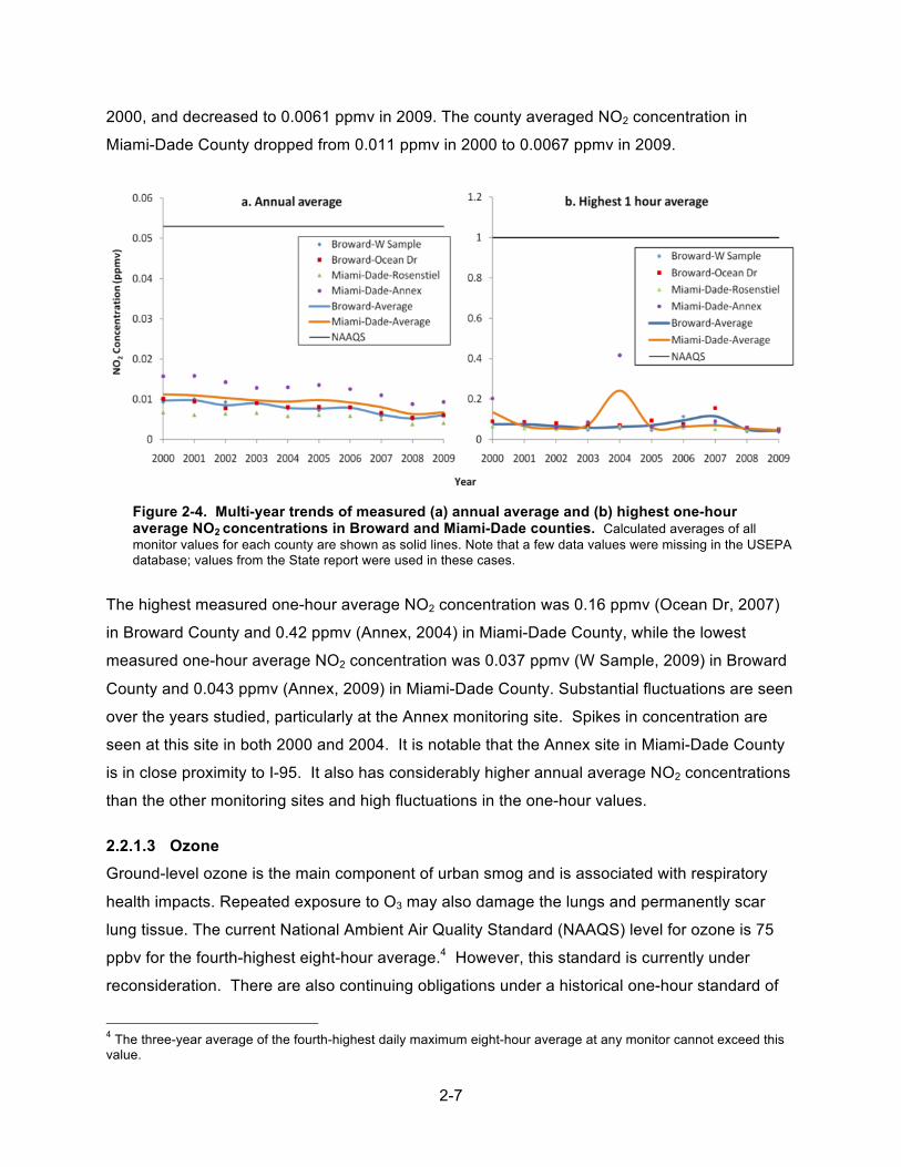
Figure 2-4. Multi-year trends of measured (a) annual average and (b) highest one-hour average NO2 concentrations in Broward and Miami-Dade counties. Calculated averages of all monitor values for each county are shown as solid lines. Note that a few data values were missing in the USEPA database; values from the State report were used in these cases.
The highest measured one-hour average NO2 concentration was 0.16 ppmv (Ocean Dr, 2007)
in Broward County and 0.42 ppmv (Annex, 2004) in Miami-Dade County, while the lowest
measured one-hour average NO2 concentration was 0.037 ppmv (W Sample, 2009) in Broward
County and 0.043 ppmv (Annex, 2009) in Miami-Dade County. Substantial fluctuations are seen
over the years studied, particularly at the Annex monitoring site. Spikes in concentration are
seen at this site in both 2000 and 2004. It is notable that the Annex site in Miami-Dade County
is in close proximity to I-95. It also has considerably higher annual average NO2 concentrations
than the other monitoring sites and high fluctuations in the one-hour values.
2.2.1.3 Ozone Ground-level ozone is the main component of urban smog and is associated with respiratory
health impacts. Repeated exposure to O3 may also damage the lungs and permanently scar
lung tissue. The current National Ambient Air Quality Standard (NAAQS) level for ozone is 75
ppbv for the fourth-highest eight-hour average.4 However, this standard is currently under
reconsideration. There are also continuing obligations under a historical one-hour standard of
4 The three-year average of the fourth-highest daily maximum eight-hour average at any monitor cannot exceed this value.

2-8
0.12 ppmv that was officially revoked April 25, 2009. Ozone (O3) is a secondary pollutant,
formed in the atmosphere through reaction of nitrogen oxides and volatile organic compounds in
the presence of sunlight. Concentrations do not typically peak in close proximity to sources in
an urban area but are expected to exhibit high levels downwind over a broader area.
Figure 2-5 shows a map of the ozone monitoring sites active sometime during the period of
study. Miami-Dade County has two O3 monitoring sites still in operation (Rosenstiel and Perdue
Med sites). The Krome Ave and Everglades sites stopped monitoring for ozone in 2003 and
2004, respectively. In Broward County, the Vista site was newly established in 2009. Sites
located within five miles of I-95 are the NE 48th St site (1.7 miles) and Ocean Dr site (3.5 miles)
in Broward County and Rosenstiel site (2.9 miles) in Miami-Dade County. All monitoring sites
except for the Everglades site use Thermo Electron/Thermo Environmental Instruments 49
series Photometric Ambient O3 Analyzer (Method 047) for ozone monitoring. The Everglades
site uses a Monitor Labs/Lear Siegler Model 8810 Photometric Ozone Analyzer. Hourly ozone
concentration data are reported.
Figure 2-5. Ozone monitoring sites in (a) Broward and (b) Miami-Dade counties. Coordinate values for the Vista site were obtained from FDEP (2009).
Multi-year trends in measured concentrations of ozone are shown in Figure 2-6. In Broward
County, the fourth highest eight-hour ozone concentration ranged from 0.055 ppmv (Vista,
2009) to 0.077 ppmv (Ocean Dr, 2006). The fourth-highest eight-hour ozone concentration in

2-9
Miami-Dade County ranged from 0.06 ppmv (Everglades, 2002) to 0.084 ppmv (Krome Ave,
2001). Some of these values are higher than the NAAQS level. The highest one-hour ozone
concentration ranged from 0.071 ppmv (W Sample, 2004 and 2007) to 0.11 ppmv (Ocean Dr,
2001, 2006 and 2008). In Miami-Dade County, it ranged from 0.069 ppmv (Everglades, 2002)
to 0.119 ppmv (Rosenstiel and Perdue Med, 2001). This latter value is very close to the one-
hour NAAQS level (now revoked). Substantial fluctuations also are observed in the data with no
apparent multi-year trends, although calculated county average concentrations in 2009 were
lower than those in 2000 for all metrics studied except the highest one-hour average.
Figure 2-6. Multi-year trends in O3 concentrations in (a, c) Broward and (b, d) Miami-Dade counties. Calculated county average values are shown with solid lines. Differences in some data values reported in collected sources were found.
2.2.1.4 Particulate matter PM consists of very small solid particles or liquid droplets that are suspended in the air.
Constituent particles vary greatly in diameter, shape and composition. USEPA categorizes and
regulates particulate matter by size due to evidence for increased health effects for small-size
particles. Health outcomes include premature death, hospital and emergency room visits, and
increased respiratory and cardiovascular symptoms. The regulated size ranges are PM10 and

2-10
PM2.5; the subscript refers to the aerodynamic diameter in micrometers of the largest particles in
the category; PM10 refers to particles with diameters less than 10 µm. Particulate matter is both
emitted directly from sources and formed in the atmosphere. Concentrations can be higher
near sources such as roadways (particularly for PM10), but also typically exhibit widespread
highs downwind of sources (particularly for PM2.5).
Figure 2-7 provides a map of PM monitoring sites in the study area during the period studied
(2000-2009). In Broward County, 10 monitoring sites have been used, but only six (Lincoln
Park, SW 70th, SW 3rd Ave, Plunkett St, Winston, Vistas) were active in 2009. Miami-Dade
County has had five sites, with three active in 2009 (PF, MF, and HF). See Table 2-2 for a listing
of the period of active monitoring for each site.
Figure 2-7. PM monitoring sites in (a) Broward and(b) Miami-Dade counties active sometime during 2000 – 2009.
Several different methods have been used for PM monitoring in the study area, as shown in
Table 2-3 and Table 2-4. This includes federal reference manual filter methods (e.g., methods
062 and 063 form PM10 and method 118 for PM2.5), co-located monitors used for quality
assurance, and continuous methods used for obtaining time-resolved data (method 079 for
PM10 and method 702 for PM2.5). To determine PM2.5 composition, each county also has one
speciation sampler (method 810). Reported data from all methods were used in the analyses
below.

2-11
2.2.1.4.1 PM10
As the current NAAQS level for PM10 is based on a 24-hour average concentration, Figure 2-8
provides the multi-year trends in the highest 24-hour average concentrations at monitoring sites
in both counties. Values range from 19 to 122 µg/m3 in Broward County; the lowest value was
observed at Lincoln Park and Winston in 2009, and the highest values were observed at
Plunkett St in 2007. In Miami-Dade County, values ranged from 31 to 64.5 µg/m3; the lowest
value was observed at MF in 2008, and the highest values were observed at MF and NW 27th
Ave in 2009 and 2003, respectively. No values exceed the current NAAQS standard of 150
µg/m3.5 Although substantial fluctuations exist, no clear multi-year trend is apparent. A peak in
PM10 concentrations was observed from 2005 – 2008 at Plunkett St and SW 3rd Ave in Broward
County, which are near the I-95 roadway.
Table 2-3. Particulate matter monitoring sites in the study area and monitoring method
County Site ID Abbreviation Monitoring Method Type Broward 12-011-0010 Lincoln Park 062 Manual Broward 12-011-0011 SW 4th Ave 062 Manual Broward 12-011-1002 SW 70th Ave N/A Manual-2
062 Manual
Broward 12-011-2004 SW 3 Ave 062 Manual 079 Continuous
Broward 12-011-3002 Plunkett St 062 Manual 079 Continuous
Broward 12-011-5002 Taft St 062 Manual Broward 12-011-5005 Winston 062 Manual Broward 12-011-6002 NW 72 Ave 062 Manual Broward 12-011-7002 NE 12th St 062 Manual Miami-Dade 12-086-0020 NW 36th St 063 Manual
Miami-Dade 12-086-1016 MF 063 Manual-2 063 Manual
Miami-Dade 12-086-3001 NW 27th Ave 063 Manual Miami-Dade 12-086-6001 HF 063 Manual Broward 12-011-0033 Vista 702 Continuous
Broward 12-011-1002 SW 70th Ave
118 Manual-2 118 Manual 810 Speciation 702 Continuous
Broward 12-011-2004 SW 3 Ave 118 Manual Broward 12-011-3002 Plunkett St 118 Manual Miami-Dade 12-086-0033 PF 118 Manual
Miami-Dade 12-086-1016 MF
118 Manual-2 118 Manual 702 Continuous 810 Speciation
Miami-Dade 12-086-6001 HF 118 Manual 702 Continuous
5 This threshold may not be exceeded more than once per year on average over three years.

2-12
Table 2-4. Explanation of PM monitoring method
PM Code Category Explanation
PM10
062 Reference Wedding & Associates/Thermo Environmental Instruments, Inc. Model 600 PM10 Critical Flow High-Volume Sampler
063 Reference Sierra-Andersen/General Metal Works Model 1200 PM10 High-Volume Air Sampler System
079 Equivalent Thermo Scientific TEOM® 1400AB PM10 Ambient Particulate Monitor or Rupprecht & Patashnick TEOM® Series 1400 and Series 1400a PM10 Monitors
PM2.5
118 Reference Rupprecht & Patashnick Partisol®-Plus Model 2025 Sequential Air Sampler or Thermo Scientific Partisol-Plus 2025 Sequential Air Sampler
702 Non-Reference TEOM Gravimetric PM2.5 Sharp Cut Cyclone (SCC) monitor with correction factor
810 Non-Reference Met-One speciation samplers (SASS) with Teflon filters
Figure 2-8. Maximum 24-hour average PM10 concentrations in (a) Broward and (b) Miami-Dade counties. Values at individual monitoring sites are averages of values from multiple monitors at each site. County averaged data are shown in solid lines.
2.2.1.4.2 PM2.5
Measured PM2.5 concentrations are shown in Figure 2-9. The current NAAQS levels are 15
µg/m3 for the annual average concentration6 and 35 µg/m3 for the 98th percentile of the 24-hour
average.7 Annual mean measured values ranged from 6.5 µg/m3 (Plunkett St, 2009) to 10.5
µg/m3 (SW 70th Ave, 2007) in Broward County and from 6.1 µg/m3 (PF, 2009) to 12.8 µg/m3
(MF, 2006) in Miami-Dade County. None of these values exceeded the NAAQS level and
concentrations appear to remain relatively constant on average over the decade. Values of the
6 The three-year average of weighted annual average concentration may not exceed this threshold at any community-oriented monitoring site. 7 The three-year average of the 98th percentile of 24-hour average concentrations may not exceed this threshold at each population-oriented monitoring site.

2-13
98th percentile of the 24-hour average ranged from 10.2 µg/m3 (Plunkett St, 2009) to 37.6 µg/m3
(SW 70th Ave, 2007) in Broward County and from 11 µg/m3 (PF site, 2009) to 28.7 µg/m3 (MF
site, 2007) in Miami-Dade County. A substantial peak in PM2.5 concentrations in Broward
County was seen in 2007 at all sites, with the highest value exceeding the NAAQS level, but
concentrations declined subsequently. Due to the fluctuations, there is no clear long-term trend;
however, calculated county average values were lower in 2009 than 2000.
Figure 2-9. Measured PM2.5 concentrations in (a) Broward and (b) Miami-Dade counties. Subplots a and b provide annual mean values at each monitoring site; c and d provide values of the 98th percentile of the highest 24-hour average concentration. Calculated county averages are shown as solid lines.
2.2.1.5 Air Quality Index The Air Quality Index (AQI) is a calculated metric of air quality that is based on the measured
values of multiple criteria pollutants (O3, PM, CO, SO2 and NO2). Its value ranges from 0 to 500,
with higher values considered more hazardous to health. Table 2-5 provides ranges of AQI
values and the associated level of health concern.
2-14
Table 2-5. Air Quality Index levels and their interpretation Air Quality Index Levels of Health
Concern
Numerical Value Meaning
Good 0-50 Air quality is considered satisfactory, and air pollution poses little or no risk.
Moderate 51-100
Air quality is acceptable; however, for some pollutants there may be a moderate health concern for a very small number of people who are unusually sensitive to air pollution.
Unhealthy for Sensitive Groups 101-150 Members of sensitive groups may experience health
effects. The general public is not likely to be affected.
Unhealthy 151-200 Everyone may begin to experience health effects; members of sensitive groups may experience more serious health effects.
Very Unhealthy 201-300 Health alert: everyone may experience more serious health effects.
Hazardous > 300 Health warnings of emergency conditions. The entire population is more likely to be affected.
*Source: http://www.airnow.gov
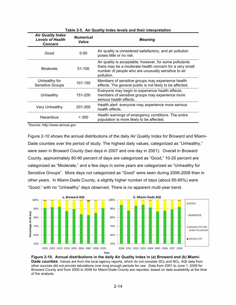
Figure 2-10 shows the annual distributions of the daily Air Quality Index for Broward and Miami-
Dade counties over the period of study. The highest daily values, categorized as “Unhealthy,”
were seen in Broward County (two days in 2007 and one day in 2001). Overall in Broward
County, approximately 80-90 percent of days are categorized as “Good,” 10-20 percent are
categorized as “Moderate,” and a few days in some years are categorized as “Unhealthy for
Sensitive Groups”. More days not categorized as “Good” were seen during 2006-2008 than in
other years. In Miami-Dade County, a slightly higher number of days (about 85-95%) were
“Good,” with no “Unhealthy” days observed. There is no apparent multi-year trend.
Figure 2-10. Annual distributions in the daily Air Quality Index in (a) Broward and (b) Miami-Dade counties. Values are from the local agency reports, which do not consider SO2 and NO2. AQI data from other sources did not provide tabulations over long enough periods for use. Data from 2001 to June 1, 2009 for Broward County and from 2000 to 2008 for Miami-Dade County are reported, based on data availability at the time of the analysis.

2-15
2.2.2 Organic pollutants
In addition to criteria pollutants, there are many other air pollutants that are emitted from
vehicles and considered harmful to health. Available data are discussed on the volatile organic
compound group and on other select pollutants.
2.2.2.1 Volatile organic compounds VOCs are a variety of gaseous chemicals that are emitted from vehicles, as well as a variety of
industrial and natural sources. Exposure to some VOCs may cause adverse health effects
ranging from minor irritation to serious effects. However, effects vary between constituents of
the group. Hence, VOCs are no longer regulated as a group with NAAQS. Instead, individual
chemicals are regulated as hazardous air pollutants (also called air toxics), discussed later.
Nonetheless, VOCs are ozone precursors, i.e., they react with nitrogen oxides in the presence
of sunlight to form ozone. Therefore, VOC monitoring occurs in support of the ozone NAAQS.
As shown in Table 2-6, VOCs are monitored at four stations in Broward County and three
stations in Miami-Dade County. However, different compounds were monitored and reported at
each station, and some compounds were added or removed each year. No group sums were
found. Additionally, some of the reported individual compounds are specifically excluded from
the VOC category in the federal regulations (40 CFR 51.100). Hence, no further analyses were
performed with the VOC monitoring data. Select air toxics associated with mobile sources were
analyzed instead, as discussed below.
Table 2-6. List of VOC monitoring sites and available data period County Site ID Abbreviation Data Available
Broward 12-011-1002 SW 70th Ave 2000-2009 Broward 12-011-2004 SW 3 Ave 2000-2008 Broward 12-011-3002 Plunkett St 2000-2008 Broward 12-011-5005 Winston 2000, 2002-2009 Miami-Dade 12-086-0020 NW 36th St 2002-2005 Miami-Dade 12-086-0029 Perdue Med 2002-2005 Miami-Dade 12-086-4002 Annex 2002-2003
2.2.2.2 Select mobile source air toxics (benzene, acetaldehyde, and 1,3-butadiene) Another group of regulated air pollutants are called hazardous air pollutants. They are not
regulated using NAAQS, but rather are regulated based on emissions and technology
requirements. A subset of this group that is associated with vehicular sources is called mobile
source air toxics. Three of these pollutants − benzene, acetaldehyde, and 1,3-butadiene − were

2-16
selected for analysis here. For these pollutants, the analysis is based on USEPA data, as local
agencies do not consistently report on these chemicals.
The monitoring sites in the study area for the selected pollutants are listed in Table 2-7. In
Miami-Dade County, no data are available after 2006. In both counties, absorption media or
canisters first capture hazardous air pollutants. Gas chromatography, followed by mass
spectrometry or flame ionization detection, are used for separation, identification, and
quantification. All data are reported as part per billion carbon (ppbc), which was converted to
ppbv for the individual compounds.
Table 2-7. Monitoring sites for the focus pollutants, pollutants monitored at each site, and period of data availability
County Site ID Abbreviation Benzene Acetaldehyde 1,3-Butadiene Broward 12-011-1002 SW 70th Ave 00-09 05-07 02-09 Broward 12-011-2004 SW 3 Ave 00-08 02-03 02-08 Broward 12-011-3002 Plunkett St 00-08 02-08 Broward 12-011-5005 Winston 00, 02-09 02-09 Miami-Dade 12-086-0020 NW 36th St 02-05 02-05 Miami-Dade 12-086-0029 Perdue Med 02-05 02-05 Miami-Dade 12-086-4002 Annex 02-03
The first mobile source air toxic studied was benzene. Benzene is present in both exhaust and
evaporative emissions from motor vehicles. Mobile sources account for approximately three-
fourths of outdoor emissions (USEPA 2000). Benzene is a known carcinogen. Short-term
exposures to benzene are associated with irritation of the skin, eyes, and upper respiratory
tract. Chronic exposures are also associated with disorders in the blood and immune system.
Figure 2-11 shows the highest measured 24-hour average and annual benzene concentrations
in Broward and Miami-Dade counties. In Broward County, 24-hour values ranged from 0.52
ppbv to 6.3 ppbv (both at the Plunkett site, 2006 and 2003, respectively). In Miami-Dade
County, they ranged from 0.58 ppbv (NW 36 Ave, 2005) to 1.3 ppbv (NW 36 Ave, 2002). The
annual benzene concentration ranged from 0.18 ppbv (Winston, 2006) to 1.6 ppbv (Plunkett,
2003) in Broward County and 0.26 ppbv (Perdue Med, 2004) to 0.53 ppbv (NW 36 Ave, 2005) in
Miami-Dade County. Overall, concentrations were lower in the second half of the decade than
the first half.

2-17
Figure 2-11. Measured benzene concentration in Broward and Miami-Dade counties. Calculated averages of all monitoring sites in a county are shown as solid lines.
Acetaldehyde was the second pollutant studied. It is emitted as a combustion by-product with
mobile sources accounting for more than half of inventoried emissions (USEPA, 2000). Short-
term exposures to acetaldehyde may cause irritation of the skin, eyes and respiratory tract.
Acetaldehyde is also an animal carcinogen; not enough data are available to classify it as a
human carcinogen. Figure 2-12 provides available measured data on acetaldehyde
concentrations in the study area. There are few data and values are scattered. The highest
values were observed at SW 70th Ave in Broward County in 2006.
Figure 2-12. Acetaldehyde concentrations in the study area.

2-18
1,3-Butadiene is also present in motor vehicle exhaust, with mobile source contributions
accounting for over half of tabulated emissions (USEPA, 2000). It is classified as a known
human carcinogen. It also may cause irritation to skin, eyes, and the respiratory tract. Figure
2-13 shows measured 1,3-butadiene concentrations in the study area. As for benzene, 1,3-
butadiene was monitored only between 2002 and 2005 in Miami-Dade County. The 24-hour
average 1,3-butadiene concentration ranged from 0.05 ppbv (SW 70th Ave, 2009) to 1 ppbv
(Plunkett, 2003) in Broward County and from 0.2 ppbv (NW 36 Ave and Perdue Med, 2005) to
0.9 ppbv (Perdue Med, 2003) in Miami-Dade County. The annual values ranged from 0.02 ppbv
(Winston, 2009) to 0.13 ppbv (Plunkett, 2003) in Broward County and from 0.06 ppbv (Perdue
Med, 2002) to 0.11 ppbv (NW 36 Ave, 2005) in Miami-Dade County. An overall downward trend
in concentrations is observed over the decade, with a peak in 2003 and 2004, particularly at the
Plunkett site.
Figure 2-13. 1,3-butadiene concentration in the study area.
2.3 Summary of baseline air quality and trends in the study area
Available ambient air monitoring data from 2000 to June 2009 of several focus pollutants,
including CO, NO2, PM10 and PM2.5, VOCs, and three mobile source air toxics (benzene,
acetaldehyde and 1,3-butadiene), were collected and compiled. Of these pollutants, data
availability for the VOC category as a group was too limited for further analysis. For each of the
other pollutants, individual monitoring site values and county average concentrations for multiple
averaging times, including those relevant to the National Ambient Air Quality Standards
(NAAQS), were calculated. Multi-year trends in time were plotted and compared with the
NAAQS levels. Data on the daily Air Quality Index (AQI) were compiled with the multi-year trend

2-19
in the annual distribution plotted. Finally, pollutant monitoring site locations were mapped
relative to the I-95 project corridor to investigate impacts of roadway proximity.
Of the pollutants studied, only ozone and PM2.5 had measured levels at some sites in Broward
County near to or slightly exceeding the NAAQS levels.8 The other criteria pollutants studied
(CO, NO2, and PM10) had measured levels substantially lower than the NAAQS levels.
However, a large fluctuation approaching the standard level during 2006-2008 was present in
the PM10 measurement data at two sites in Broward County near the I-95. No ambient standard
levels are applicable to the mobile source air toxics studied.
Impacts on concentrations of the proximity of monitoring sites to the I-95 roadway also were
qualitatively assessed. CO, NO2, and PM10 all have substantial primary (direct) emissions from
sources and mobile sources contribute a large portion of their emissions amounts. Hence,
concentrations often are higher near to sources, particularly large roadways. Correspondingly,
the highest measured concentrations of these pollutants were observed at sites in close
proximity to the I-95 (Annex and Lincoln Park for CO, Annex for NO2, and SW 3 Ave and
Plunkett for PM10). These monitoring sites may be useful as indicators of the effects of the
managed lane project. Since O3 and PM2.5 have substantial contributions to their concentrations
from secondary formation (i.e., chemical reactions in the atmosphere of emitted pollutants), the
local monitoring site location relative to the any source is not expected to be very important.
Additionally, the data do not show higher concentrations at sites in close proximity to the
corridor.
Regarding multi-year trends in air quality, no clear trend (in increasing or decreasing
concentrations) was seen in the O3, PM2.5, or PM10 measurement data, though county average
values were lower in 2009 than in 2000 for all averaging times except for the maximum 1-hr
average ozone concentration. For CO and NO2, the multi-year trend plots suggest slightly
decreasing levels in the study area over the decade. For the mobile source air toxics studied,
measurement data suggest lower concentrations of benzene and 1,3-butadiene in the later half
of the decade. Data for acetaldehyde are too sparse to discuss trends. Distributions of the AQI
suggest that the overall air quality with respect to criteria pollutants is better in Miami-Dade
County than in Broward County. Only a few days during the decade in either county were
categorized as “Unhealthy for Sensitive Groups,” and very few as “Unhealthy” generally (and in
Broward County alone). 8 Note that this does not imply regulatory nonattainment with the NAAQS. The criteria for nonattainment involve specific data requirements, multi-year distribution parameters, and other factors. Rather, this is a comparison of the levels measured with those corresponding to the standard.

3-1
3 MOBILE SOURCE EMISSIONS (OBJECTIVE 2): METHODS AND FINDINGS
As a step toward understanding impacts of the I-95 managed lane project on air quality, it is
important to determine the change in mobile source emissions of air pollutants due to the
implementation of the corridor project. To do this, a transportation corridor traffic micro-
simulation model (CORSIM) was selected and applied to simulate corridor traffic flow
characteristics (traffic volumes and link speeds). Simulations were performed for scenarios
representing conditions prior to the implementation of the managed lane project and after the
implementation of Phases 1A and 1B of the project. Emissions then were calculated using the
simulated traffic flow characteristics and emissions factors from the USEPA’s MOBILE6.2
emissions factor model. Changes in emissions rates resulting from the managed lane project
were analyzed, with a focus and assessing impacts on bus transit emissions. The focus
pollutants for emissions calculations were carbon monoxide, nitrogen oxides, PM10,
hydrocarbons, and benzene. Detailed information on these methods and the resultant findings
are discussed below.
3.1 Transportation corridor simulation modeling
This study adopted a Traffic Software Integrated System Corridor-microscopic Simulation
software package (generally referred as CORSIM). CORSIM is a traffic simulation model
developed by the Federal Highway Administration (FHWA) and models traffic movements in
time, with second-by-second resolution. The model assumes that individual vehicles travel
based on car-following and lane-changing theories. Based on the car-following theory, a
follower vehicle will maintain a desired headway between itself and the in-front vehicle, reacting
to changes in speed of that vehicle. The behavior of the vehicle is dependent on how the car
that leads it responds to traffic control and other conditions. Thus, the software is capable of
simultaneously modeling integrated networks using commonly accepted vehicle and driver
behaviors.
CORSIM was selected to simulate the operation performance of the HOT lanes and measure
potential changes relevant to vehicle emissions, as it is considered as the most cost-effective
option with affordable workloads to build networks. Additionally, model configurations for the
I-95 HOT lane implementation were available from FDOT. It should also be noted that CORSIM
was recommended by the Committee to Review EPA's Mobile Source Emissions Factor
(MOBILE) Model (TRB 2000). Additionally, the Minnesota Department of Transportation has

3-2
applied CORSIM to determine whether the implementation of a managed lane might degrade
conditions on general-purpose lanes (GPLs).
3.1.1 CORSIM model setup for I-95 study corridor
The I-95 express lane project contains three phases − 1A, 1B, and 2. Phase 1A (northbound on
I-95 from I-395 in downtown Miami to the Golden Glades Interchange) was opened in
December 2008, and Phase 1B (southbound on I-95 from the Golden Glades Interchange to I-
395 in downtown Miami) was opened in January 2010. The study area is shown in Figure 3-1a,
including the location of the project on I-95 between I-395 and the Golden Glades Interchange.
Figure 3-1. I-95 study corridor and corresponding CORSIM network.
CORSIM models for the I-95 express lanes project were obtained from FDOT District 6 and
include a configuration representative of conditions prior to the I-95 express lane project, with
Study Area

3-3
one HOV lane and four GPLs, for both the morning and afternoon peak hours (07:00-09:00 and
15:30-17:30, respectively). This configuration was used as the pre-implementation baseline
scenario for this analysis. A configuration representative of the conditions after Phase 1A and
Phase 1B for both peak-hour ranges also was available, with two HOT lanes and four GPLs.
This was adopted as the post-implementation “after” scenario in this analysis. Other than the
differences mentioned above, the geometric infrastructure in each configuration is the same.
Figure 3-1b shows the basic simulation model for the corridor. The HOV lane was coded with
the same links as the GPLs, and the HOT lanes were coded with separate links.
CORSIM volume input data were obtained from the Sunguide Transportation Management
Center (TMC) for the year 2007, before the implementation of HOT lanes. The volume data from
2008 cannot be used due to construction at the site. Each model contains eight 15-minute
intervals. Total input volumes and mode-share were kept constant in both scenarios. The split of
the volumes on the HOT lanes and GPLs was based on the ratio of accurate traffic on two
segments from the TMC data.
Regarding buses, the I-95 Express bus (95X) is the only transit service on I-95 between
downtown Miami and the Golden Glades Interchange. The bus schedules differ for northbound
and southbound lanes during peak hours (7:00 – 9:00, and 15:30 – 17:30). The bus route and
schedule was added to the CORSIM models, with volumes shown in Figure 3-2. Buses use
only the HOV and HOT lanes, not the GPLs. During morning peak hours, a total of 21 buses
travel on the northbound lanes and 31 buses travel on the southbound lanes. During the
afternoon peak hours, 29 buses travel northbound, while six buses travel southbound.
Figure 3-2. Bus volumes for northbound and southbound lanes during each time period.
0
1
2
3
4
5
6
1 2 3 4 5 6 7 8
No.
of B
uses
Tra
velli
ng
Time Period
Northbound A.M. Northbound P.M. Southbound A.M. Southbound P.M.

3-4
3.1.2 CORSIM Calibration
Calibration and validation form a crucial element of the simulation task. Because of the
stochastic nature of traffic, variations between the model and observed data always are
expected, and the onus is upon the model user to establish the desired reliability level and the
validation effort required to achieve it. For the baseline scenario, the available model
configuration and validation were reviewed and adopted. Since the after scenario models were
built prior to the implementation of the project, additional calibration was needed on these. To
do this, the research team conducted field data collection by real-time video recording as Phase
1A construction was being completed. Four video cameras were installed on a vehicle. Two
cameras on the top monitored the front and back geometry and traffic; another two on each side
of the vehicle captured the traffic closest to the vehicle. The collected geometric information
includes the number of general-purpose lanes and express lanes, locations of sequential
entrances and exits, and number of lanes on on-ramps and off-ramps. Those segments that
were still under construction (Phase 1B) could not be included in validation efforts. Results
confirmed that the after scenario models properly represented the implementation of the I-95
express lanes project.
In addition, the Geoffrey E. Havers (GEH) method was used to calibrate the results. The GEH
method is the criteria to calibrate freeway models in the Traffic Analysis Tools Program of the
FHWA, which was developed by the Wisconsin Department of Transportation (WDOT 2002;
FHWA 2004). For each individual link flow, the acceptable calculated GEH value should be less
than 5.0. The GEH statistic is computed as:
GEH = [2(E-V)2/(E+V)]0.5
where E is the model estimated volume and V is the field count volume. Traffic volume data
were obtained from detectors of the Sunguide Transportation Management Center for morning
peak hours and afternoon peak hours at 15-minute intervals. Ten locations, shown in Figure 3-
3, were available when comparing the real detector data and CORSIM models. The GEH
criteria were calculated for the after scenario model for eight periods in the morning peak hours
from 07:00 to 09:00 and eight periods in the afternoon peak hours from 15:30 to 17:30. Based
on the calculated GEH values, 98.75 percent of the segments in the morning and 95 percent of
the segments in the afternoon meet the accepted calibration target criteria.

3-5
Figure 3-3. Phase 1A-NB 1-95 volume validation sites.
3.1.3 Discussion of mode share impacts of managed lane implementation
This project evaluated the changes in emissions due to converting one HOV lane to two HOT
lanes on I-95 while four GPLs stayed the same. Since emissions can vary by vehicle type, it is
important to understand changes of mode-share due to the lane conversion. HOV lanes are
intended to encourage the use of alternate modes of transportation, such as transit, carpool,
and vanpool, by providing an exclusive lane with decreased travel times. However, several
previous studies have found that HOV lanes in the U.S. are underused due to the poor transit
services, the scarcity of potential carpool matches, restricted accesses in some regions to high-
occupancy vehicles carrying only two people, and inconvenience related to trip chaining (Kwon
and Varaiya 2006; Evans 2009; Burris et al. 2009; Burris and Goel 2010). The concept of using
HOT lanes is to increase the use of HOV lanes and provide the unused capacity of the HOV
lanes to vehicles with fewer occupants than the HOV threshold. Thus, this capacity also would
improve performance of the GPLs through displacement of some single occupancy vehicles
(SOV) to HOT lanes by paying a toll. During recent years, HOT lanes have been considered an

3-6
option for increasing the operational efficiency of managed lanes over existing HOV lanes. To
determine the likelihood of mode share changes due to the study project, current implemented
managed lane facilities in the U.S were examined.
Nine HOT/Express Toll facilities have been completed and eight HOT lanes are under
development as of 2010 in the U.S. HOT lane implementations and their findings related to the
change of mode-share are summarized in Table 3-1. Nine managed lane facilities, commonly
HOT or Express Toll lanes, have been implemented in six states (California, Colorado, Florida,
Minnesota, Texas, and Utah). No significant change in mode-share was found. This is
consistent with the information from the “Transportation Emission Guidebook” (Dierkers et al.
2002). According the guidebook, about a one percent reduction in automobile use was
estimated based on a case study. Based on the limited impact, mode-share was kept constant
for both simulation models prior to and after the managed lane implementation.
Table 3-1. Findings of changes of mode-share due to current HOT implementation
Managed Lane Change of Mode Share
SR-91 Express Lanes, Orange County, CA
• Based on limited bus and commuter rail, it was concluded that 91 express lanes did not take patrons from corridor transit service.
• From 1994 through 1999, the counts of PM peak HOV2 vehicles remained essentially unchanged.
I-15 Express Lanes, San Diego
• Switching to or from transit riders was not observed. • Very few carpools were broken up by HOT lanes implementation.
Katy and Northwest, Houston
• Based on a state survey, responses showed riders loyal to transit mode. • In the evening peak, only 1% of HOT riders are diverted from HOV modes.
I-394 Express Lanes, Minneapolis
• Comparing data from 2004 to 2005, no change was found regarding mode changes of previous transit users.
• No negative effect on carpooling was found due to implementation of MnPASS HOT lanes.
I-25 Express Lanes, Denver
• No conclusions regarding effects on transit use were made since change in ridership of concerned routes was very small (<0.5% over a year).
• Changing rules from HOV to HOT did not have a large impact on most mode choices.
I-15 Express Lanes, Salt Lake City
• No information or data available regarding mode-share.
SR-167 HOT Lanes, Seattle • No evidence showed HOT lane impact on transit ridership.
I-95 Express Lanes, Miami
• Transit mode remained relatively consistent - 3.6% in 2008, 3.5% in 2009. • Express Lane has limited impact on private auto users with regard to mode share.

3-7
3.1.4 CORSIM Results: Managed lane performance
Each simulation model was repeated 10 times, and the output data were calculated by taking
the average. Performance results are discussed, with a focus on impacts on bus transit.
Average speed results of the pre-implementation (baseline) and post-implementation (after)
scenarios in the northbound direction are plotted in Figure 3-4. Results from both scenarios
show that average speeds on the managed lanes (HOV/HOT) were slightly higher than on the
GPLs. Prior to the HOT lane conversion, the I-95 corridor experienced heavy congestion, with
speeds as low as 16 mph on the pre-existing GPLs. Although the average link speeds for both
the HOV lane and GPLs were around 40 to 50 mph during morning peak hours, they decreased
to 20 to 30 mph for the afternoon peak hours. After implementation of the HOT lanes, speeds
increased to 40 to 50 mph. This represents a significant increase of travel speeds on I-95
northbound during the afternoon peak hours. Therefore, implementation of HOT lanes relieved
congestion on the I-95 corridor, especially for the peak hours. This result is consistent with the
previous TMC data. Simulation results also are consistent with the midyear evaluation report on
the I-95 corridor (FDOT 2009).
Figure 3-4. Average speeds on managed lanes and GPLs for each time interval during afternoon peak hours (15:30-17:30) for northbound lanes only.
Regarding transit buses, the implementation of HOT lanes relieves congestion and enhances
bus speeds. An average of nine minutes savings for each bus traveling northbound during the
afternoon peak hours is seen in model results, shown in Figure 3-5. However, for the
southbound direction, only two minutes’ savings are seen for all the buses on HOT lanes as
10 15 20 25 30 35 40 45 50 55 60
1 2 3 4 5 6 7 8
HOV Lane GPLs HOT Lanes Pre-existing GPLs 15-minute time interval number
Ave
rage
Spe
ed (m
ph)

3-8
compared to the HOV lane. These results are consistent with the transit evaluation report for 95
Express (FTA 2009), which found that the express lanes on I-95 have a significant impact on
the northbound travel times of I-95 Express buses between downtown Miami and the Golden
Glades interchanges.
3.2 Emissions estimation
To estimate emissions changes resulting from the case study project, simulated results of traffic
parameters from the CORSIM transportation model were input into the MOBILE6.2 emissions
factor model to obtain emission factors for all vehicles and for buses alone. The generated
emissions factors were resolved by roadway link, pollutant, month and year. The emissions
factors then were combined with extrapolated annual traffic data to calculate the annual
emissions, as discussed below.
Figure 3-5. Time savings for northbound and southbound lanes during each 15-minute time interval of morning and afternoon peak hours simulated.
3.2.1 Emission factors
MOBILE6.2 was used to calculate emissions factors relevant to the corridor project.
MOBILE6.2 is an established model for estimating pollutions emitted from on-road vehicles.
Several pollutants can be addressed by MOBILE6.2, including hydrocarbons (HC), NOx, CO,
PM, and select hazardous air pollutants. MOBILE6.2 has been widely used by federal, state,
regional, and local planning agencies and organizations in many applications to evaluate motor
vehicle emissions, including for State Implementation Plans (SIPs), National Environmental
0 1 2 3 4 5 6 7 8 9
10 11 12
1 2 3 4 5 6 7 8
Tim
e S
avin
gs (m
in)
15-minute time interval number
Northbound A.M. Northbound P.M. Southbound A.M. Southbound P.M.

3-9
Protection Act (NEPA) analysis, transportation planning and conformity analysis, and
environmental impact analysis.9
To use results from the CORSIM model for the calculation of emission factors using
MOBILE6.2, some processing of the CORSIM results was required. This processing included
mapping of the CORSIM vehicle classes to the MOBILE6.2 classes, as the two models have
different vehicle classes. The mapping of categories of classes from CORSIM to MOBILE6.2 is
shown in Table 3-2 (FHWA 2007; EPA 2001). The vehicle distribution percentages for
comparable categories for the before-and-after scenarios also are listed. Note that these were
adjusted to include bus counts. For example, buses are assumed to travel only in the HOT
lanes, and not in the GPLs in the after scenario. Vehicle type distribution data from the 29
counting sites located on the ramps of I-95 modeling section also were obtained and compared
with the vehicle distributions used in CORSIM and they were found to be similar. Distribution
percentages from CORSIM then were allocated proportionally to the constituent MOBILE6.2
categories based on the default 2009 vehicle miles traveled (VMT) fraction in MOBILE 6.2 (EPA
2001; EPA 2004), as shown in Table 3-3. Also, CORSIM only includes the freeway facility.
Hence, only freeway facilities were modeled with MOBILE6.2, by using VMT distribution input
files.
Table 3-2. Mapping of vehicle class categories between CORSIM and MOBILE6.2 model, with vehicle distribution percentages based on CORSIM output
CORSIM class IDs
CORSIM vehicle descriptions
Corresponding MOBILE6.2
classesa
Vehicle distribution percentages
Before scenario,all lanes
After scenario
GPLs HOT lanes
1, 2, 8,9 Low- and high performance passenger cars, carpool and
individual occupancy
LDV, LDT1, LDT2, LDT3
LDT4 95.859% 96.0% 95.5975%
3 Single-unit truck HDV2B - HDV7 1.2382% 1.24% 1.2348%
4, 5 Semi-trailer truck with medium and full loads HDV8A 2.3965% 2.40% 2.3899%
6 Double-bottom trailer truck HDV8B 0.3595% 0.36% 0.3585% 7 Conventional bus HDBS, HDBT 0.1469% 0.00% 0.4192%
aDescriptions of MOBILE6.2 class identifiers are given in Table 3-2. GPLs are general-purpose lanes. HOT lanes are high-occupancy/toll lanes.
In addition to vehicle class mapping, processing of speed data also was required. CORSIM
simulates average speeds for 15-minute time intervals on each roadway link for the four rush 9 MOBILE6.2 currently is being replaced for regulatory analysis with the MOVES model.

3-10
hours of a typical weekday. To account for the diurnal variations in speed on each link in
MOBILE6.2, external “Speed VMT” files were created for each link using 14 speed bins.
Speeds for hours corresponding to the CORSIM simulation were determined by averaging the
15-minute interval CORSIM link speed output data. Speeds during hours not modeled by
CORSIM were assumed to be at the speed limit (55 mph).
Fuel and meteorological parameters used in MOBILE6.2 calculations were extracted from the
National Mobile Inventory Model County Database (EPA 2005). Monthly varying fuel parameters
for Miami-Dade County were used. Monthly varying meteorological parameters also were used.
For 2009, the 20-year (1981-2000) average of hourly temperature and humidity were used due
to lack of available data for that year at the time of analysis. Default data were used for other
parameters, including the diesel sale fraction distributions among vehicle types.
Table 3-3. MOBILE6.2 vehicle classes and distribution percentages used for emissions calculations
MOBILE6.2 class ID
MOBILE6.2 vehicle class description
Default 2009
distribution
Before scenario
distribution
After scenario
GP lane distribution
HOT lane distribution
1 LDV Light-Duty Vehicles (Passenger Cars) 36.6863% 40.2687% 40.3279% 40.1588%
2 LDT1 Light-Duty Trucks 1 8.6891% 9.5376% 9.5516% 9.5116% 3 LDT2 Light-Duty Trucks 2 28.9371% 31.7627% 31.8095% 31.6761% 4 LDT3 Light-Duty Trucks 3 8.9191% 9.7900% 9.8044% 9.7633% 5 LDT4 Light-Duty Trucks 4 4.0996% 4.4999% 4.5065% 4.4876%
6 HDV2B Class 2b Heavy-Duty Vehicles 3.8896% 0.7157% 0.7167% 0.7137%
7 HDV3 Class 3 Heavy-Duty Vehicles 0.3800% 0.0699% 0.0700% 0.0697%
8 HDV4 Class 4 Heavy-Duty Vehicles 0.3200% 0.0589% 0.0590% 0.0587%
9 HDV5 Class 5 Heavy-Duty Vehicles 0.2400% 0.0442% 0.0442% 0.0440%
10 HDV6 Class 6 Heavy-Duty Vehicles 0.8699% 0.1601% 0.1603% 0.1596%
11 HDV7 Class 7 Heavy-Duty Vehicles 1.0299% 0.1895% 0.1898% 0.1890%
12 HDV8A Class 8a Heavy-Duty Vehicles 1.1199% 2.3965% 2.4000% 2.3899%
13 HDV8B Class 8b Heavy-Duty Vehicles 3.9796% 0.3595% 0.3600% 0.3585%
14 HDBS School Buses 0.2000% 0.0979% 0.0000% 0.2795%
15 HDBT Transit and Urban Buses 0.1000% 0.0490% 0.0000% 0.1397%
16 MC Motorcycles 0.5399% 0.0000% 0.0000% 0.0000%

3-11
MOBILE6.2 modeling was performed for the following scenarios: 1) baseline scenario, 2)
general-purpose lanes for the after scenario, and 3) HOT lanes for the after scenario. Five
pollutants were included: HC, CO, NOx, PM10, and benzene. Evaporative emissions other than
running evaporative emissions were omitted because these activities are not modeled by
CORSIM. Seven types of particulate emissions were included: exhausted SO4, exhaust lead,
organic carbon and elemental carbon from diesel vehicle exhaust, total carbon, and brake-wear
and tire-wear particles.
Emissions factors output from MOBILE6.2 were resolved by year, month, pollutant, and link.
Emissions factors for buses alone also were obtained to calculate bus emissions. Annual
average emission factors for 2009 are listed in Table 3-4 to Table 3-8. Note that it is assumed
that there are no buses traveling on the GPLs in the after scenario.
3.2.2 Daily and annual traffic estimation
To estimate annualized emissions, traffic information is needed throughout the day and year.
Since CORSIM simulates only four rush hours of a typical day, external diurnal and annual
profiles were applied, as discussed here.
Diurnal and monthly traffic patterns, shown in Figure 3-6, were derived from 2007 hourly vehicle
count data obtained from a traffic monitoring site located on I-95 (site ID: 860331) The count site
is approximately five miles from the north end of the section of I-95 modeled by CORSIM. Data
for the northbound and southbound lanes were averaged separately to obtain hourly average
traffic counts for both directions. Average daily total traffic counts for 12 months also were
calculated.
Figure 3-6. Diurnal and monthly traffic count distributions for northbound and southbound lanes.

3-12
Table 3-4. All-vehicle annual average emissions factors (g/mile) for the before scenario
Pollutant 2005 2006 2007 2008 2009 Benzene 0.0323 0.0287 0.026 0.0228 0.0205
CO 15.43 13.49 12.6 11.64 10.83 HC 1.31 1.22 1.15 1.07 0.98
NOx 1.46 1.33 1.21 1.11 1.01 PM10 0.0398 0.0377 0.0361 0.0344 0.033
Table 3-5. All-vehicle annual average emission factors (g/mile) for after scenario general-purpose lanes
Pollutant 2005 2006 2007 2008 2009 Benzene 0.0318 0.0282 0.0256 0.0225 0.0202
CO 15.65 13.67 12.77 11.8 10.98 HC 1.27 1.18 1.11 1.03 0.95
NOx 1.45 1.32 1.2 1.1 1 PM10 0.0388 0.0369 0.0353 0.0337 0.0324
Table 3-6. All-vehicle annual average emission factors (g/mile) for after scenario HOT lanes
Pollutant 2005 2006 2007 2008 2009 Benzene 0.0317 0.0281 0.0255 0.0224 0.0201
CO 15.63 13.65 12.75 11.77 10.95 HC 1.26 1.17 1.1 1.03 0.95
NOx 1.5 1.37 1.25 1.14 1.05 PM10 0.0415 0.0393 0.0374 0.0356 0.0342
Table 3-7. Annual average emissions factors for buses alone for the before scenario (g/mile)
Pollutant 2005 2006 2007 2008 2009 Benzene 0.0042 0.0036 0.0031 0.0027 0.0024
CO 3.19 3.01 2.74 2.42 2.14 HC 0.39 0.34 0.29 0.25 0.22
NOx 18.75 17.83 16.83 15.69 14.6 PM10 0.63 0.5 0.4 0.31 0.26
Table 3-8. Annual average emission factors (g/mile) for buses alone for after scenario HOT lanes
Pollutant 2005 2006 2007 2008 2009 Benzene 0.0039 0.0034 0.0029 0.0025 0.0022
CO 2.97 2.8 2.56 2.25 1.99 HC 0.36 0.31 0.27 0.23 0.21
NOx 18.97 18.04 17.02 15.88 14.77 PM10 0.63 0.5 0.4 0.31 0.26

3-13
Hourly traffic count data also were obtained from 12 counting sites located in Miami-Dade
County. After excluding missing and poor quality data, the county average diurnal and monthly
profiles were calculated and compared with the profiles calculated based on data site 860331.
As shown in Figure 3-7, the diurnal patterns were very similar, but the monthly patterns were
somewhat different. Because it is located on I-95, the diurnal and monthly pattern from site
860331 was considered more representative and was used for further analysis.
Figure 3-7. Comparison of diurnal and monthly traffic count distributions between site 860331 and the Miami-Dade County average.
A total daily traffic volume for emissions calculations was extrapolated from the CORSIM data
by dividing the sum of the CORSIM traffic counts by the fraction of the total measured average
daily count represent by the hours in the model, i.e.:
where Td is the total daily traffic volume, th is the CORSIM derived traffic count for hour h, and fh
is the measurement data derived fraction of the total count for hour h. To obtain monthly
varying traffic counts, this value was proportionally extrapolated using the monthly distribution
from the measurement data.
3.2.3 Emissions
Daily emissions for each month were calculated by multiplying the MOBILE6.2 emissions factor
for the corresponding month with the roadway link length and the estimated daily traffic counts.
Monthly total emissions then were estimated by multiplying the daily emissions for each month
with number of days in that month. Monthly total emissions were summed together to get annual
total emissions. For the after scenario, emissions from HOT lanes and GPLs were summed to
€
Td =thh∑fhh∑

3-14
obtain the total emissions for the after scenario. Estimated 2009 annual emissions for the five
pollutants are shown in Table 3-9.
Figure 3-8 shows a comparison of the relative annual emissions for the five chosen pollutants
before and after the HOT lane implementation. As seen in the figure, the HOT lane
implementation led to increased total emissions for all pollutants considered except HCs, though
increases were small. Emissions from buses alone did, however, decrease.
Table 3-9. Estimated 2009 annual emissions (tons)
Pollutants Before scenario total
After scenario total
Before scenario buses alone
After scenario buses alone
CO 6657.19 6892.08 2.12 1.91 NOx 623.21 640.36 14.27 14.17 HC 604.07 595.01 0.22 0.2
Benzene 12.58 12.65 0.0024 0.0021
PM10 20.28 20.69 0.25 0.24
Figure 3-8. Estimated relative emissions before and after managed lane implementation.
The before scenario emissions have been set to the reference value of 1 for this comparison.
3.2.4 Discussion of factors influencing emissions changes
As seen above, emissions from the corridor for all scenarios increased somewhat for the after
scenario. To understand these increases, the parameters influencing emissions were
investigated and uncertainties are discussed here.
Two primary constituent parameters can affect estimated emissions: the amount of vehicle
miles traveled and emissions factors (mass of pollutant per vehicle mile traveled). If either of
these parameters increases independently, emissions will increase. Table 3-10 shows the
change in emissions along with the change in each of the constituent factors. Annual miles

3-15
travelled increase by 2 percent, on average. For CO, NOx, and PM10, the emissions factors
increase (on average), consistent with the change in emissions. Conversely, for the HCs the
emissions factors decrease (on average), counteracting the increase in miles traveled. For
benzene, the emission factors decrease is less, leading to smaller overall increases in
emissions.
Table 3-10. Percentage change in 2009 annual emissions and primary parameters contributing to emissions for after vs. before scenario
Pollutant Annual emissions Emissions factorsa Annual miles traveleda CO 3.5% 1.2%
2% NOx 2.8% 1.3% PM10 2.0% 0.74% HCs -1.5% -3.7% Benzene 0.54% -1.7%
aNote that emissions are calculated on a link-by-link basis using disaggregated emissions factors (over 100,000), volumes, and link lengths. The values listed here are based on simple averages of individual values to demonstrate overall differences.
3.2.5 Discussion of emissions uncertainties
It is useful to consider uncertainty in the emissions, as they are functions of the traffic conditions
that may be impacted by project. Therefore, uncertainties in emissions factors and vehicle
miles traveled are discussed here.
Emissions factors are functions of vehicle speed and vehicle type. To understand the
associated uncertainties, emissions factors output from CORSIM’s internal emission factor
calculator were considered in comparison to MOBILE6.2 emissions factors. A sensitivity
analyses also was performed on impacts of speed on emissions factors.
CORSIM is capable of calculating emissions factors internally for CO, NOx and HCs for each
link and vehicle class type. As a comparison to the MOBILE6.2 emissions, CORSIM emission
factors were produced based on the default emissions factor tables in the model. On average,
emission factor values output by CORSIM decreased for the after scenario compared with the
before scenario. Since this result is the opposite of that found using MOBILE6.2, a comparison
of the effects of important traffic conditions was performed. Specifically, sensitivity analyses
were performed on the effects of speed using both MOBILE6.2 and CORSIM.
As discussed in Section 3.1.4, travel times on the corridor improved after the implementation of
the HOT lanes. Specifically, speeds in the northbound lanes increased from about 20-30 mph
to 45-50 mph during the afternoon rush hours. Since emission factors are a function of speed,
this can impact emissions. Sensitivity analysis with speed varying in both MOBILE6.2 and
CORSIM indicate different impacts of speed on the emissions factors for the different models.

3-16
In MOBILE6.2, the change in speed had little impact on the emissions factors for CO and NOx,
as shown in Figure 3-9a, due to the shape of the emission factor curve. However, for the
CORSIM emission factors, shown in Figure 3-9b, emission factor values consistently decrease
as speed increase over the range of speed improvements found here. This leads to a
difference in the direction of the emission results. Since MOBILE6.2 emissions factors have
been reviewed extensively, it is expected that their dependence on speed is more
representative. However, this difference leads to an uncertainty in the emissions results.
Figure 3-9. Relative emission factors for all vehicles from (a) CORSIM and (b) MOBILE6.2. Values are relative to value at 10 mph.
Vehicle type distribution also can affect emission factors. For the MOBILE6.2 estimation,
average corridor vehicle distributions were used for all vehicles except buses to calculate
emissions factors. (Buses were allocated only to the HOV and HOT lanes). In CORSIM, vehicle
distributions can change temporally in each lane. If vehicles with higher emissions rates (e.g.,
trucks) are traveling in a manner different from other vehicles (i.e., on poorer-performing lanes)
such that their speeds are significantly different from other vehicles, this could result in some
error in emissions factor generation using an average corridor vehicle distribution. However,
speed improvements seen in model results did not significantly affect the MOBILE6.2 emissions
factors; hence, this is not expected to have a big impact. Additionally, although improvements in
emissions for buses were found here, their contribution to the overall vehicle distribution is small
enough that changes in their emissions do not have a significant impact on overall emissions
changes.
The age of the fleet can affect emissions factors, as newer vehicles often have new
technologies that reduce emissions. A large portion of the fleet in the study area consists of
rental cars, which are replaced relatively quickly. Additionally, buses in Broward County also
a b

3-17
are replaced more quickly than in many areas. Therefore, emissions estimated using default
fleet age characteristics may overestimate emissions for the study area (both before and after
implementation of the managed lanes.)
In addition to emissions factors, uncertainties in estimated vehicle miles traveled can impact
emissions. Although input vehicle volumes to CORSIM were kept constant between the
baseline scenario and after scenario modeling, CORSIM is a stochastic model. This resulted in
an increase in the total vehicle count during peak hours for the after scenario by 3.1 percent for
the northbound direction and 1.9 percent for southbound direction. Increases in link vehicle
volumes resulted in increases in estimated vehicle miles traveled. Increased VMT results in
increased estimated emissions for the after scenario relative to the baseline case. More
important, VMT on the corridor may change due to improvements in the corridor speed
performance, as more vehicles will choose to use the corridor rather than surface streets. This
effect could not be considered here, as vehicle volumes entering the corridor are an input
parameter to corridor models like CORSIM. A model of the entire surrounding transportation
network would be required to consider this impact. However, overall effects on emissions could
be balanced due to decreases in emissions on other roadways.
3.3 Summary of emissions calculations and results
To calculate emissions changes associated with HOT lane implementation, transportation
corridor micro-simulation modeling and emissions estimation were performed. CORSIM was
selected as the transportation model and was used to simulate traffic conditions before the
implementation of the HOT lane on I-95 (baseline scenario) and after the implementation of
Phases 1A and 1B of the project (after scenario). Results of the micro-simulation modeling
indicate that the average speeds on the corridor were improved and congestion was reduced
after HOT lane implementation. With regard to transit, bus travel times were improved.
Traffic condition and infrastructure data from CORSIM then were used to generate MOBILE6.2
emissions factors and to calculate emissions changes associated with the HOT lane
implementation. Total estimated annual emissions of CO, NOx, PM10, and benzene showed
small increases after the implementation of the HOT lanes, while HCs showed decreases. CO
showed the highest percentage increase of 3.5 percent, while HC emissions decreased by 1.5
percent. Regarding transit specifically, emissions from buses decreased after the
implementation of the HOT lane. The overall increased emissions for criteria pollutants were
found to be due to modeled increases in corridor vehicle volumes and emissions factors.

3-18
However, it should be noted that there is significant uncertainty in estimated vehicle volume
changes. Overall, the magnitude of the emissions changes is small, with substantial uncertainty.

4-1
4 AIR QUALITY EFFECTS (OBJECTIVE 3): METHODS AND FINDINGS
To investigate the impacts of the I-95 HOT lane project on air quality, changes in air pollutant
concentrations due project implementation were estimated. Specifically, an atmospheric
dispersion model was selected and used to simulated pollutant concentrations in the study area.
4.1 Dispersion modeling methods
4.1.1 Review and selection of dispersion models Several atmospheric dispersion modeling systems were reviewed as candidate models for this
work, including CALINE (3 and 4), CAL3QHC and CAL3QHCR, AERMOD, CALPUFF, and
HYROAD. Characteristics of each model and previous performance for roadway modeling
studies are discussed .
CALINE (3 and 4) are the third and the fourth generation steady-state Gaussian line source
dispersion models developed by the California Department of Transportation. Both models can
be used in uncomplicated terrains (Jungers et al. 2006). CALINE3 was designed to model inert
pollutant concentrations within 150 meters of a roadway under free-flow conditions. Idling
emission at intersections are not represented in the model. Up to 20 roadway links and 20
receptors can be used into CALINE3 (Benson 1979). CALINE4 extended the modeling distance
to 500 meters and employed a mixing zone concept to characterize pollutant dispersion very
close to roadways. Simple modeling options for intersections, street canyons, and parking
facilities also have been incorporated into CALINE4 (Benson 1989). CALINE4 has the ability to
model pollutants emitted from vehicle acceleration and deceleration; however, the algorithm
does no fully represent current vehicle technology (Carr et al. 2007). CALINE3 and CALINE4
have been used to model roadway emissions for many years because they are very easy to use
and have low computational requirements. Previous studies using CALINE (Marmur and
Mamane 2003; Levitin et al. 2005; Jones et al. 1998) have show good performance, and
modeling results have been evaluated (Jungers et al. 2006; Benson 1992). Limitations of
CALINE 3 and 4 include the limited number of sources and receptors allowed, the small
allowable size of modeling domain, and source elevation limitation to below 30 feet. The
performance of both models is poor under low wind conditions (less than one m/s) (Benson
1992). Additionally, as steady-state models, they cannot capture fast varying atmospheric
patterns.
CAL3QHC and CAL3QHCR are models based on CALINE3 with an added queuing algorithm at
signalized intersections. CAL3QHCR additionally includes processing of meteorological data for

4-2
a whole year, a complete mixing height algorithm, representation of variable traffic, and added
concentration averaging algorithms (Eckhoff et al. 1995). Because these models are based on
CALINE3, they also can be used to model inert pollutant concentration near roadways.
However, they are also limited in the representation of the height of sources and very low wind
speed conditions (Eckhoff et al. 1995). Additionally, the traffic delay and capacity data within the
model are based on 1985 data, which may not be applicable for current conditions (Carr et al.
2007). The performance of these models is somewhat mixed in a number of studies. Some
studies have obtained favorable results under open area and moderate traffic flow conditions
(Abdul-Wahab 2004, Kho et al. 2007; Cain and Welch 2004). However, other evaluation studies
have found the performance to be poor (Chen et al. 2008).
AERMOD is a steady-state Gaussian plume model developed by the USEPA and the American
Metrological Society. It was designed to replace the ISCST3 model and is recommended by the
EPA as a preferred model for dispersion modeling of inert pollutants under short range (up to 50
km) and steady-state conditions (Jungers et al. 2006). AERMOD has several input data
processors, including a meteorological data processor (AERMET), a terrain data processor
(AERMAP), and a surface characteristics processor (AERSURFACE). AERSCREEN, a
screening version of AERMOD, also is built into the model. In modeling scenarios involving
terrain interaction and building downwash, BPIPPRIME is also available. AERMOD has the
ability to model a combination of point, area, and volume sources under all terrain conditions,
and it incorporates some state-of-the-science features such as a building wake algorithm
(PRIME). An updated planetary boundary layer turbulence parameterization also enables the
treatment of elevated sources and complex terrain. AERMOD is considered an accurate
dispersion model for regulatory purposes (Jungers et al. 2006) and has been used in mobile
source pollutant dispersion modeling in numerous studies (e.g., Radonjic et al. 2003; Cook et al.
2008; Wang et al. 2009; Venkatram et al. 2009). Comparison between AERMOD modeling
results and monitoring results in these studies showed good agreement, generally within a
factor of 2. Roadways are represented as area sources in these studies, with the length-to-
width ratio kept below 10 in most studies. Comparison between AERMOD and ISCST3, a widely
used historical dispersion model, also showed improved performance. However, for long-range
pollutant transport and non-steady conditions, the CALPUFF model is recommended (Jungers
et al. 2006).
CALPUFF is a non-steady state Lagrangian puff model. Although the model is privately owned
and maintained, the USEPA recommends using CALPUFF for long-range pollutant transport

4-3
and non-steady atmosphere patterns. Compared with other models discussed here, CALPUFF
incorporates many enhanced features, including transport over water, coastal interaction, puff
splitting, slug (elongated puff) transport, and wind shear effects. Because it is a non-steady
state model, it is able to handle spatial and temporal varying metrological conditions (Scire et al.
2000). CALPUFF also has the ability to model simple chemical reaction mechanisms.
CALPUFF has many pre- and post- processors, including CALMET, a meteorological pre-
processor that provides hourly three-dimensional wind and temperature fields, and CALPOST, a
post-processor for analysis of concentration. CALPUFF requires much more input data than the
other models discussed here. Studies that have used CALPUFF for roadway modeling show
mixed results. Modeled concentrations have been found to be within a factor of 2 of the
monitored concentrations for some studies (Radonjic et al. 2003; Cohen 2004; Song et al.
2006), while results from other studies are less favorable (Hatzopoulou 2008). Due to the
complexity of the model, more evaluation is needed in near field cases (Brode et al. 2008).
HYROAD is an integrated model that includes a traffic module, an emissions module, and a
dispersion module. The dispersion algorithm is based on CALPUFF (Carr et al. 2007).
HYROAD was designed to predict hourly CO concentrations near intersections (up to 500
meters), but also can be used for other inert pollutants. The puff algorithms in HYROAD also
include several features specifically designed for roadways, such as vehicle-induced flows,
vehicle wake effects, and enhanced vertical dispersion over roadways. The traffic module in
HYROAD is based on NETSIM (a part of the CORSIM model), which simulates individual
vehicle drive patterns, including accelerations and decelerations. In the emissions module,
MOBILE5 or MOBILE6 emission factors can be applied. Emission factors do not account for
acceleration or deceleration rates, but are based on calculated average speeds on roadway
links (Carr et al. 2002). Up to 60 receptors and 50 roadway links can be represented in
HYROAD (Carr et al. 2002). According to Carr et al. (2007), HYROAD has shown better
performance when compared with CAL3QHC. Limitations include the small spatial extent of the
dispersion representation (less than 500 meters) and the limited focus on intersections.
Additionally, HYROAD is a relatively new model, with few evaluation studies.
The focus of the current study is to investigate impacts of the managed lane project on air
quality in the case study area. Therefore, a model capable of representing concentrations over
a large area is needed. Several of the models reviewed here, including CALINE 3 and 4,
CAL3QHC (and R), and HYROAD cannot represent concentrations over the study area domain.
CALPUFF is a promising model for this type of analysis due to its enhanced features and ability

4-4
to represent non-steady conditions. However, it is data and computationally intense, and the
enhanced features likely are not necessary for understanding average conditions sought here.
Additionally, it has not been adequately evaluated for near-field conditions. Therefore,
AERMOD was chosen for this work due to its wide use and performance in air quality modeling
of roadway emissions, its capabilities for modeling larger domains, and its lower computational
and data requirements relative to CALPUFF.
4.1.2 AERMOD dispersion simulations
To determine impacts of the I-95 managed lane project on air quality in the study area,
AERMOD simulations were performed for both the baseline scenario and after scenario cases
discussed previously. Several types of input data and processing were required. These include
calculation of emissions sources, selection and processing of appropriate meteorological data,
configuration of the receptor grid, and selection of appropriate dispersion parameters. Methods
used are discussed below.
Pollutant emissions from the case study I-95 roadway section modeled by CORSIM were
represented, as shown in Figure 4-1. The coordinates of all roadway link nodes were obtained
from the CORSIM configuration and converted to UTM coordinates. Roadway links were input
into AERMOD as area sources. Each roadway link was expanded to a rectangle, whose width
was calculated using the number of lanes times the width of each lane. The length was set as
the link length. A maximum aspect ratio of 10 was applied to each source (EPA 2004b), with
links subdivided when necessary. The emission rates of each source for each pollutant modeled
in the AERMOD simulation were set to vary by season and hour of the day. For each season,
the daily emissions values discussed in Chapter 3 in the constituent months were averaged to
obtain the average daily emissions for the season. The daily profile then was used to allocate
the calculated daily emissions to each hour of the day.
For meteorological data, five years (2005-2009) of data from the Miami International Airport
station were used to represent conditions in the study area. Surface monitoring data on
temperatures, winds and cloud cover were retrieved from the Integrated Surface Hourly
Database through the National Climatic Data Center (ftp://ftp.ncdc.noaa.gov/pub/data/noaa).
Upper air sounding data on pressure, temperature, relative humidity, and upper-level winds
were collected from NOAA/ESRL Radiosonde Database (http://www.esrl.noaa.gov/raobs/). The
data were processed by AERMET to produce hourly resolved meteorological fields.

4-5
Figure 4-1. Section of I-95 modeled.
Necessary modeling parameters include the initial vertical dispersion parameter and surface
characteristics. The initial vertical dispersion parameter was used to account for the initial
mixing of the pollutants during emissions (EPA 1995), which can be important in situations
where pollutants are mechanically generated, such as vehicle emissions (EPA 2004). A value of
2 was used consistent with previous literature (Venkatram et al. 2009). Surface characteristics
such as noontime albedo, Bowen ratio, and surface roughness length were used to estimate
boundary layer turbulence. The range of the three parameters and the values selected are
shown in Table 4-1 (EPA 1999; EPA 2004; Paine 1987). In consideration of the sub tropical
climate characteristics in Broward and Miami-Dade counties, a summer value of albedo and
Bowen ratio were applied.
Table 4-1. Surface characteristic parameters Surface characteristics Range Value used Albedo 0.1 (thick forests) - 0.65 (fresh snow) 0.16 (summer) Bowen ratio 0.1 (over water) - 10.0 (desert) 1 (summer) Surface roughness length 0.01 m (calm water) - 1 m (forest or urban area) 1 (urban)
The receptor grid provides the locations at which concentrations are calculated by AERMOD. It
was chosen to cover Broward County and the northern part of Miami-Dade County, as shown in
Figure 4-2. To characterize the pollution concentration near I-95, the receptor network was

4-6
denser near to the roadway and less dense farther away. Maximum resolution was 100 m and
minimum resolution was 5 km.
Figure 4-2. Receptor grid. Subplot a provides an overview of the receptors in the entire modeling domain, and b provides the network near the I-95 project section.
Once pre-processing and parameter selection were complete, AERMOD simulations were
performed for each of the five years of meteorological data for both baseline and after scenario
emissions. Concentrations of nitrogen oxides, carbon monoxide, and benzene were estimated.
Specifically, the first and second highest one-hour average and eight-hour average
concentrations, as well as annual average concentrations at each receptor location, were
calculated and extracted from the model output. Differences between concentrations for the
baseline and after scenario were also calculated. Results were interpolated and mapped using
ArcGIS for analysis.
4.2 Results: Estimated pollutant concentrations
Table 4-2 and 4-3 provide a summary of estimated concentration ranges for the baseline and
after scenarios for each pollutant. All estimated CO concentrations are well below regulatory
standard levels. No standard level for NOx exists; however, in comparison to the NO2 standard
level, most modeled levels are low, but the highest modeled one-hour average NOx values are
of the same magnitude as the NO2 standard level. It should be noted that the percentage of
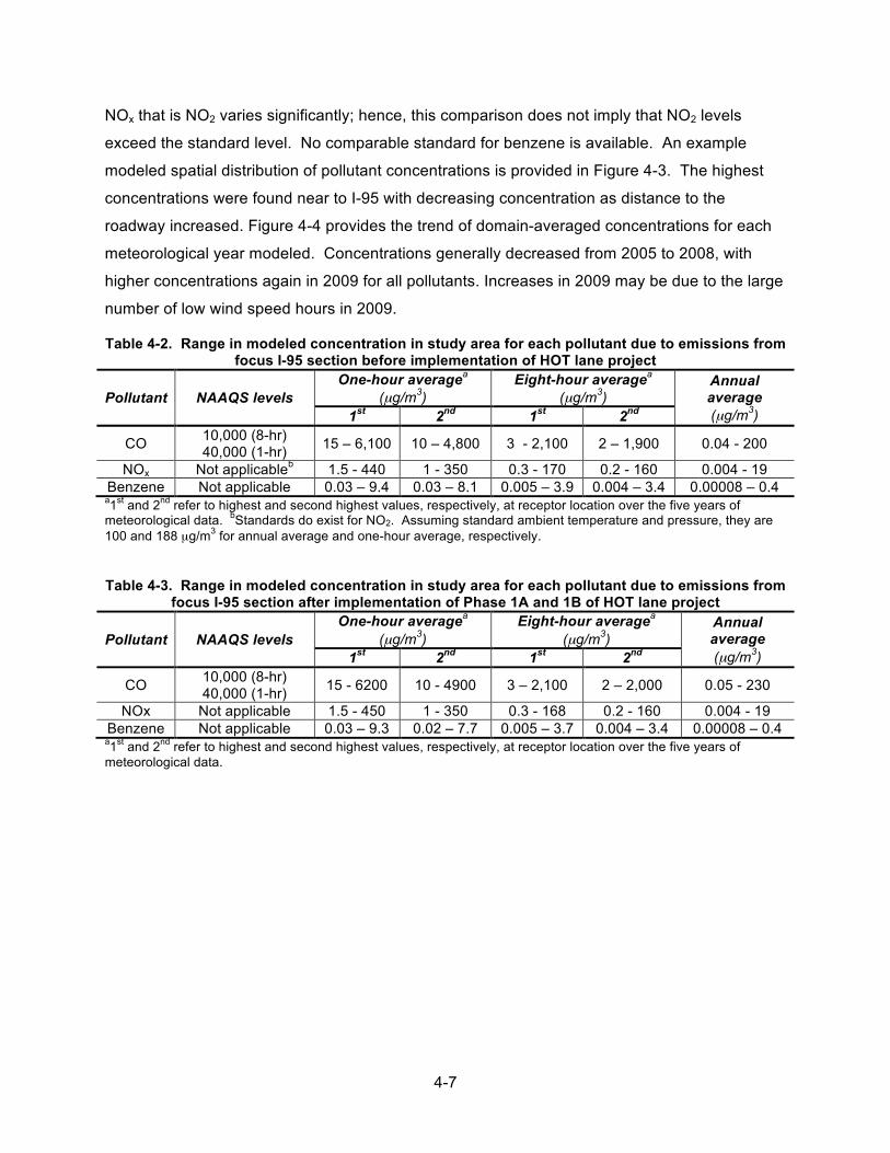
4-7
NOx that is NO2 varies significantly; hence, this comparison does not imply that NO2 levels
exceed the standard level. No comparable standard for benzene is available. An example
modeled spatial distribution of pollutant concentrations is provided in Figure 4-3. The highest
concentrations were found near to I-95 with decreasing concentration as distance to the
roadway increased. Figure 4-4 provides the trend of domain-averaged concentrations for each
meteorological year modeled. Concentrations generally decreased from 2005 to 2008, with
higher concentrations again in 2009 for all pollutants. Increases in 2009 may be due to the large
number of low wind speed hours in 2009.
Table 4-2. Range in modeled concentration in study area for each pollutant due to emissions from focus I-95 section before implementation of HOT lane project
Pollutant NAAQS levels One-hour averagea
(µg/m3) Eight-hour averagea
(µg/m3) Annual average (µg/m3) 1st 2nd 1st 2nd
CO 10,000 (8-hr) 40,000 (1-hr) 15 – 6,100 10 – 4,800 3 - 2,100 2 – 1,900 0.04 - 200
NOx Not applicableb 1.5 - 440 1 - 350 0.3 - 170 0.2 - 160 0.004 - 19 Benzene Not applicable 0.03 – 9.4 0.03 – 8.1 0.005 – 3.9 0.004 – 3.4 0.00008 – 0.4 a1st and 2nd refer to highest and second highest values, respectively, at receptor location over the five years of meteorological data. bStandards do exist for NO2. Assuming standard ambient temperature and pressure, they are 100 and 188 µg/m3 for annual average and one-hour average, respectively. Table 4-3. Range in modeled concentration in study area for each pollutant due to emissions from
focus I-95 section after implementation of Phase 1A and 1B of HOT lane project
Pollutant NAAQS levels One-hour averagea
(µg/m3) Eight-hour averagea
(µg/m3) Annual average (µg/m3) 1st 2nd 1st 2nd
CO 10,000 (8-hr) 40,000 (1-hr) 15 - 6200 10 - 4900 3 – 2,100 2 – 2,000 0.05 - 230
NOx Not applicable 1.5 - 450 1 - 350 0.3 - 168 0.2 - 160 0.004 - 19 Benzene Not applicable 0.03 – 9.3 0.02 – 7.7 0.005 – 3.7 0.004 – 3.4 0.00008 – 0.4 a1st and 2nd refer to highest and second highest values, respectively, at receptor location over the five years of meteorological data.

4-8
Figure 4-3. Modeled pollutant concentrations in study area due to emissions from focus I-95 section prior to the implementation of HOT lanes project. Subplots a - c are for CO, d – f are for NOx, and g - i are for benzene. Concentration averaging times plotted are highest one-hour average (a, d, g), highest eight-hour average (b, e, h), and annual average (c, f, i) over the five-year meteorological study period.
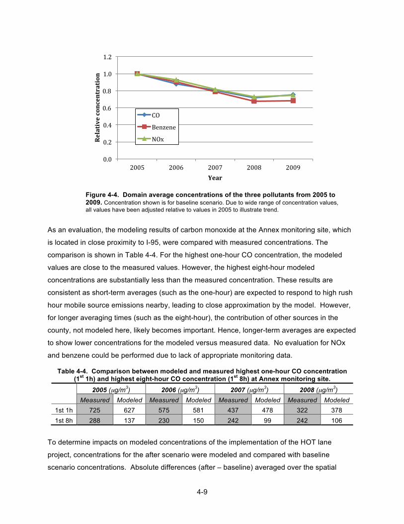
4-9
Figure 4-4. Domain average concentrations of the three pollutants from 2005 to 2009. Concentration shown is for baseline scenario. Due to wide range of concentration values, all values have been adjusted relative to values in 2005 to illustrate trend.
As an evaluation, the modeling results of carbon monoxide at the Annex monitoring site, which
is located in close proximity to I-95, were compared with measured concentrations. The
comparison is shown in Table 4-4. For the highest one-hour CO concentration, the modeled
values are close to the measured values. However, the highest eight-hour modeled
concentrations are substantially less than the measured concentration. These results are
consistent as short-term averages (such as the one-hour) are expected to respond to high rush
hour mobile source emissions nearby, leading to close approximation by the model. However,
for longer averaging times (such as the eight-hour), the contribution of other sources in the
county, not modeled here, likely becomes important. Hence, longer-term averages are expected
to show lower concentrations for the modeled versus measured data. No evaluation for NOx
and benzene could be performed due to lack of appropriate monitoring data.
Table 4-4. Comparison between modeled and measured highest one-hour CO concentration (1st 1h) and highest eight-hour CO concentration (1st 8h) at Annex monitoring site.
2005 (µg/m3) 2006 (µg/m3) 2007 (µg/m3) 2008 (µg/m3)
Measured Modeled Measured Modeled Measured Modeled Measured Modeled 1st 1h 725 627 575 581 437 478 322 378 1st 8h 288 137 230 150 242 99 242 106
To determine impacts on modeled concentrations of the implementation of the HOT lane
project, concentrations for the after scenario were modeled and compared with baseline
scenario concentrations. Absolute differences (after – baseline) averaged over the spatial
0.0
0.2
0.4
0.6
0.8
1.0
1.2
2005 2006 2007 2008 2009
Relative concentration
Year
CO
Benzene
NOx

4-10
domain are provided in Table 4-5. Example difference distributions are shown in Figure 4-5
through Figure 4-7. For all CO and NOx for the averaging times studied, modeled domain
average concentrations increased slightly after the managed lane implementation versus before
implementation. For benzene, the sign of the difference in domain average concentrations
depends on the averaging time considered. Difference plots also indicate that differences are
positive (higher for the after scenario) throughout most of the study domain. However, small
negative differences were observed north of the focus I-95 section for all pollutants. An analysis
of the vehicle miles traveled on the corridor indicates that these decreases are due to the spatial
distribution of VMT. In the after scenario, the north section of the corridor experienced lower
traffic volumes (and, hence, lower emissions). Overall, all difference were very small,
representing less than 3 percent of the baseline scenario concentrations for all receptors.
Table 4-5 Domain-averagea differences in modeled pollutant concentrations for each pollutant due to implementation of HOT lane project.
Positive values indicate increases for after scenario, while negative values indicate decreases.
Pollutant
Highest one-hour average
(µg/m3)
Highest eight-hour average
(µg/m3) Annual average
(µg/m3) CO 18 4.9 3.1 NOx 1.1 0.27 0.033 Benzene 0.0006 -0.0013 0.0001
aSimple domain average of concentration at all receptors in domain. Since receptor network is denser near roadway, concentrations near roadway carry heavier weight in average.
Figure 4-5. Estimated changes in carbon monoxide concentrations due to implementation of HOT lane project. Plots are interpolated from absolute differences at each receptor site for after scenario vs. baseline scenario. Subplot a provides change in highest one-hour average concentration, while subplot b provides change in five-year average annual benzene concentration.

4-11
Figure 4-6. Estimated change in nitrogen oxides concentrations due to implementation of HOT lane project. Plots are interpolated from absolute differences at each receptor site for after scenario vs. baseline scenario. Subplot a provides change in highest one-hour average concentration, while subplot b provides change in five-year average annual nitrogen oxides concentration.
Figure 4-7. Estimated change in benzene concentrations due to implementation of HOT lane project. Plots are interpolated from absolute differences at each receptor site for after scenario vs. baseline scenario. Subplot a provides change in highest one-hour average concentration, while subplot b provides change in five-year average annual benzene concentration.

4-12
4.3 Summary and discussion of air quality results
The AERMOD Gaussian dispersion model was selected and used to estimate pollutant
concentrations in the study area due to emissions from the case study I-95 corridor.
Concentrations of carbon monoxide, nitrogen oxides, and benzene were estimated. AERMOD
simulations were performed using emissions for the baseline scenario (before the
implementation of HOT lanes on the corridor) and for the after scenario (after the
implementation of Phases 1A and 1B of the HOT lane project). All modeled concentrations of
CO were substantially lower than the comparable regulatory standard level. (No directly
comparable standard exist for NOx or benzene.) As expected, concentrations near the
emissions corridor were substantially higher than farther from the corridor. On average and
throughout most of the study spatial domain, higher concentrations of CO and NOx were
estimated after HOT lane implementation, though the magnitude of the increase is small.
Although concentrations of benzene also increased slightly in part of the study domain, a large
area had decreasing concentrations. For all pollutants, concentrations near the north end of the
corridor decreased due to a change in the spatial distribution of vehicle volumes. Overall, all
concentrations differences between the after and baseline scenarios were small.

5-1
5 INTEGRATED DISCUSSION AND SUMMARY
5.1 Impact of the I-95 HOT lanes project on bus transit Corridor simulation results suggest improvement in corridor speeds after implementation of the
HOT lanes, particularly in the northbound lanes during the afternoon peak hours. This reduction
in congestion led to improved travel times for buses. It is expected that improved bus travel
times could improve the perception and use of transit on the corridor.
5.2 Impacts of the I-95 HOT lanes project on air quality
The total annual estimated emissions of CO, NOx, PM10, and benzene showed slight increases
after the implementation of the managed lane project. Emissions of HCs showed a slight
decrease. Emissions changes were quite small, with the highest total emissions change for CO
of 3.5 percent. For buses alone, total emissions decreased significantly after the
implementation of the HOT lanes. Further analysis suggests that the link traffic volumes in the
CORSIM modeling were slightly higher in the after scenario compared to the baseline scenario,
contributing to the emissions change. Speed improvements on the corridor did not result in
decreased overall MOBILE6.2 emissions factors. Emissions factors decreased on average for
HCs and benzene only. Uncertainties regarding volume changes associated with HOT lane
implementation, coupled with the small magnitude of estimated changes in emissions, suggest
important uncertainties in the overall impacts of the project on emissions.
Consistent with the emissions results, modeled concentrations of CO and NOx showed slight
increases after the HOT lane implementation throughout much of the study area. The benzene
concentrations results are more mixed. The highest concentration differences were found close
to the I-95 corridor for the shortest averaging times. Concentration to the north of the corridor
deceased for all pollutant due to changes in the emissions distribution. Compared to the
magnitude of the overall concentration values, the change in air quality due to the
implementation of the management lane project is quite small.
5.3 Implications for impacts of managed lane projects A purpose of managed lane projects is to encourage vehicle sharing and reduce congestion by
applying access restrictions to certain lanes. Upon successful implementation, increases are
expected for the average speed on the roadway and the percentage of high occupancy vehicles
(and transit ridership) in the fleet. The results here are consistent with increases in roadway
performance regarding speed, with concomitant improvements in transit bus travel times.

5-2
Regarding air quality impacts, the increase of average speed on the roadways may lead to the
reduction of mobile source emissions for some pollutants, but not all of them (USEPA 2002;
Granell et al. 2004; Tang et al. 2004). Emissions of benzene, volatile organic compounds and
particulate matter have shown a negative relationship with increasing average speed. Thus,
reduction in congestion may lead to emission reduction for these pollutants. The correlations
between speed and the emissions for other pollutants, such as carbon monoxide, are more
complicated; the estimated all-vehicle average CO emission rate exhibited a minimum in the
range of speeds found on the corridor studied here, resulting in increases on either side of that
minimum. Regarding vehicle distributions, if vehicle sharing and transit ridership increase
significantly due to the implementation of the managed lane project, the total VMT could
decrease and the reduction of mobile source emissions could occur. However, significant mode
change has not yet been observed substantially in many managed lane projects across the U.S.
(discussed in Chapter 3); hence, these benefits are still unclear. More work is needed to
understand mode share impacts.
5.4 Issues with combining transportation modeling and air pollution methods Since transportation models and air quality models were developed out of separate disciplines
for different purposes, their combination requires translation. For the purposes of air quality
modeling, transportation modeling provides traffic information such as vehicle temporal behavior
(e.g., speeds and vehicle flow rates) and characteristics (vehicle types) necessary for emissions
estimation. Two issues were identified during the translation between CORSIM and
MOBILE6.2/AERMOD. First, vehicle classification methods are different between the
transportation simulation model and the emission estimation model. Better mapping of vehicle
class distributions between models would be helpful for the emission estimation. Additionally,
the time scales traditionally relevant to each type of study are distinct. CORSIM simulated
traffic during rush hours. This is not sufficient for long-term air quality modeling purposes, which
requires allocation of this short time scale data to the annual time scale. The extrapolation
required introduces uncertainties in the emissions and concentration estimation.
5.5 Final Summary
The air quality and bus transit performance impacts of a case study managed lane project were
studied. The case study project involved the implementation of HOT lanes on a corridor of I-95
near Miami. Conditions after Phase 1B of the project were compared to conditions prior to
project implementation. Methods from the transportation and air pollution fields were combined
to investigate impacts. Specifically, air quality monitoring data were collected from multiple

5-3
agencies to analyze the baseline and temporal trends in air quality in Broward and Miami-Dade
counties. Using corridor micro-simulation transportation modeling with CORSIM, traffic
conditions before and after the implementation of the HOT lanes project were simulated.
Corridor performance, with a particular focus on transit bus speeds and travel time, were
analyzed. Using traffic data from the CORSIM simulation results and MOBILE6.2 emission
factor estimation, emissions of CO, NOx, PM10 HC, and benzene before and after the
implementation of the HOT lane project were calculated. Dispersion modeling using AERMOD
was performed for select pollutants to investigate the air quality impact of the managed lane
project.
Air quality monitoring data were collected from reports and databases of relevant local to federal
agencies. Monitoring data from 2000 through June 2009 of O3, NO2, CO, PM2.5 and PM10,
VOCs, and selected air toxics in Broward and Miami-Dade counties were compiled.
Concentrations of pollutants other than O3 and PM2.5 were well below the comparable NAAQS
levels. The highest measured concentrations of the latter two pollutants approached or slightly
exceeded the standard levels at some monitors. Over the decade, an apparent decreasing
trend in concentrations was observed for CO, NO2, benzene, and 1,3-butadiene, while no
apparent trends were observed for other pollutants.
Emissions from the study corridor of primary pollutants associated with vehicle sources (CO,
NOx, PM10, HCs, and benzene) before and after the implementation of the managed lane
project were calculated. Results of the corridor traffic simulations show improvements in the
speed performance of the corridor, particularly in the northbound lanes during afternoon peak
hours. Bus travel times, in particular, were reduced. Comparison of emissions before and after
implementation of the HOT lane project indicates small increases in total emissions of all
pollutants studied except HCs after the implementation of the project. However, differences are
small with important uncertainties.
Concentrations of three select pollutants (CO, NOx, and benzene) resulting from corridor
emission before and after the HOT lane implementation were estimated using AERMOD
dispersion modeling. Differences in concentrations were small overall but indicate increases in
the concentration throughout much of the study domain, with a small area of decreases near the
north end of the study corridor. Concentrations and differences were largest near the I-95
corridor. Impacts for benzene were more mixed, with a large area of the domain experiencing
decreased concentrations. Overall, results suggest relatively small impacts of the HOT lane
project on air quality for this case study.

5-4
Finally, methods for assessing air quality impacts of managed lane projects were developed and
demonstrated here. Although useful and necessary for understanding general trends in air
quality in the study area, available monitoring data did not clearly show an apparent signature of
the managed lane project. In future work, comparative statistical analysis of time series data at
select monitoring sites may be useful in attributing the trends found here. Conversely, the
combination of corridor transportation modeling with air pollution modeling allowed estimation of
highly-resolved spatial distributions of pollutant concentrations due the managed lane
implementation. This approach likely would be useful for additional case studies under varying
conditions, necessary for generalizability. Important sources of uncertainties in understanding
and modeling air quality impacts of managed lane projects also were identified. Specifically,
improvements in methods are needed for 1) estimation of network level impacts on vehicle
volume redistribution, 2) emissions factor model representation of speed effects, and 3) tools for
effectively translating between transportation and air pollution models. Nonetheless, the results
found and methods demonstrated provide an important step towards understanding the impacts
of managed lanes and other corridor-level projects on air quality.

6-1
6 REFERENCES
Abdul-Wahab, S. A. 2004. An application and evaluation of the cal3qhc model for predicting carbon monoxide concentrations from motor vehicles ear a roadway intersection in Muscat, Oman. Environmental Management 34(3): 372–382.
Benson, P. E. 1979. CALINE3 - A versatile dispersion model for predicting air pollutant levels near highways and arterial streets. Office of Transportation Laboratory, California Department of Transportation.
Benson, P. E. 1989. CALINE4 - A dispersion model for predicting air pollutant concentrations near roadways. Division of New Technology and Research, California Department of Transportation.
Benson, P. E. 1992. A review of the development and application of the CALINE3 and CALINE4 models. Atmospheric Environment 26B-3, 379-390.
Brode, R. W., and B. Anderson. 2008. Technical Issues related to CALPUFF near-field applications. U.S. Environmental Protection Agency.
Burris, W. M., H. D. Ungemah, M. Mahlawat, and S. M. Pannu. 2009. Investigating the impact of tolls on high-occupancy-vehicle lanes using managed lanes. Transportation Research Record 2099: 113-122.
Burris, W. M., and R. Goel. 2010. Mode choice due to HOV to HOT conversions. Presented at 89th Transportation Research Board Annual Meeting, Washington D.C.
Cain, C. J., and S. Welch. 2004. Cal3qhcr modeling analysis for Missoula, Montana, redesignation to carbon monoxide NAAQS attainment. Retrieved from: http://www.co.missoula.mt.us/airquality/AirProgramProjects/CORedesignation/pdfs/BrooksSouthRussellModelling.pdf.
Carr, E. L., R. G. Johnson, and R. G. Ireson. 2002. User’s guide to Hyroad − The Hybrid Roadway Intersection Model. Systems Applications International, Inc., and KLD Associates, Inc.
Carr, E. L., D. A. Ernst, A. Rosenbaum, G. Glass, and S. Hartley. 2007. Analyzing, documenting, and communicating the impacts of mobile source air toxic emissions in the NEPA process. ICF International.
Chen, H., S. Bai, D. Eisinger, D. Niemeier, and M. Claggett. 2008. Modeling uncertainties and near-road PM2.5: A comparison of CALINE4, CAL3QHC and AERMOD. Retrieved from: http://aqp.engr.ucdavis.edu/Documents/2008-Chen-Dispersion-Model-Report-PM-final.pdf.
Cohen, J., R. Cook, C. R. Bailey, and E. Carr. 2004. Relationship between motor vehicle emissions of hazardous pollutants, roadway proximity, and ambient concentrations in Portland, Oregon. Environmental Modeling and Software 20: 7-12.
Committee to Review EPA's Mobile Source Emissions Factor (MOBILE) Model. 2000. Modeling mobile-source emissions. Board on Environmental Studies and Toxicology, Transportation Research Board, National Research Council.
Cook, R., V. Isakov, J. S. Touma, W. Benjey, J. Thurman, E. Kinnee, and D. Ensley. 2008. Resolving local-scale emissions for modeling air quality near roadways. Journal of the Air & Waste Management Association 58: 451-461.
Dierkers, G., E. Silsbe, S. Stott, S. Winkelman, and M. Wubben. 2002. CCAP transportation emissions guidebook - Part one: Land use, transit & travel demand management. Center for Clean Air Policy. Retrieved from: http://www.ccap.org/images/guidebook/ CCAP_Transportation_Guidebook_Part1.pdf
Dowling, R., R. Ireson, A. Skabardonis, D. Gillen, and P. Stopher. 2005. Predicting Air Quality Effects of Traffic Flow Improvements. NCHRP Report 535. Washington D.C.: Transportation Research Board.

6-2
Eckhoff, P. A., and T. N. Braverman. 1995. CAL3QHCR user's guide. office of air quality planning and standards. U.S. Environmental Protection Agency.
Evans J. J. 2009, Exploring travel preferences of transit and shared ride users in a proposed HOV to HOT conversion. Cambridge Systematic, Inc., TRB Planning Applications Conference, Houston, Texas.
Federal Highway Administration. 2003. FHWA guide for HOT lane development, FHWA-OP-03-0009, http://www.its.dot.gov/JPODOCS/REPTS_TE/13668.html, accessed March 3th, 2010.
Federal Highway Administration. 2007. Traffic analysis toolbox volume IV: Guidelines for applying CORSIM microsimulation modeling software. Retrieved from: http://ops.fhwa.dot.gov/trafficanalysistools/tat_vol4/vol4_guidelines.pdf.
Federal Transit Administration. 2009. Miami Urban Partnership Agreement (UPA) project phase 1A - Transit evaluation report.
Florida Department of Environmental Protection. 2009. Broward County 2009 air monitor site. Retrieved from: http://www.dep.state.fl.us/air/FLAQS.
Florida Department of Transportation. 2009. Final 95 Express midyear report: Project status for Urban Partnership Agreement.
Georgia Transportation Partner Public Relations. 2010. Case study: California’s SR 91 express lanes - First private, congestion-priced toll lanes reduce trip times in congested southern California. Retrieved from: http://www.georgiatransportationpartners.com/case_study_sr91etl_lanes.pdf.
Godish, T. 2004. Air Quality – 4th Edition. Lewis Publishers. Hatzopoulou, M. 2008. An integrated multi-model approach for predicting the impact of
household travel on urban air quality and simulating population exposure. Department of Civil Engineering, University of Toronto.
Hinds, W. C. 1999. AerosolTechnology: Properties, Behavior, and Measurement of Airborne Particles. Second Edition. John Wiley & Sons, Inc.
Jones, G., N. Gonzalez-Flesca, R. S. Sokhi, T. McDonald, and M. Ma. 1998. Measurement and interpretation of concentrations of urban atmospheric organic compounds. Environmental Monitoring and Assessment 52: 107-121.
Jungers, B. D., D. Niemeier, T. Kear, and D. Eisinger. 2006. A survey of air quality dispersion models for project level conformity analysis. Retrieved from: http://aqp.engr.ucdavis.edu/Documents/Dispersion-Model-Report-Fnl.pdf.
Kho, F. W. L., P. L. Law, S. H. Ibrahim, and J. Sentian. 2007. Carbon monoxide levels along roadway. Journal of Environmental Science and Technology 4(1): 27-34.
Kwon J., and P. Varaiya. 2006. Effectiveness of California’s High Occupancy Vehicle (HOV) System. University of California, Berkeley. Retrieved from: http://paleale.eecs.berkeley.edu/~varaiya/papers_ps.dir/HOV_summitv6
Levitin, J., J. Harkonen, J. Kukkonen, and J. Nikmo. 2005. Evaluation of the CALINE4 and CARFMI models against measurements near a major road. Atmospheric Environment 39: 4439-4452.
Marmur A., and Y. Mamane. 2003. Comparison and evaluation of several mobile-source and line-source models in Israel. Transportation Research Part D: Transport and Environment 8(4): 249-265.
National Research Council. 2004. Air quality management in the United States. National Academies Press, Washington, D.C.
Nesamani S. K., L. Chu, G. M. McNally, and R. Jayakrishnan. 2006. Estimation of vehicle emissions by capturing traffic variations. Presented 86th TRB Annual Meeting, Washington, D.C.

6-3
New Zealand Ministry for the Environment. 2000. Health effects of five common air contaminants and recommended protective ranges. Retrieved from: http://www.mfe.govt.nz/publications/air/5-common-air-oct00.pdf.
Orange County Transportation Authority. 2009. SR-91 Express Lanes in Orange County, California. Retrieved from: http://www.91expresslanes.com.
Paine, R. J. 1987. User's guide to the CTDM Meteorological Preprocessor (METPRO) Program. EPA-600/8-88-004, U.S. Environmental Protection Agency, Research Triangle Park, North Carolina.
Replogle, M. 1995. Appendix E. Minority statement. In Expanding Metropolitan Highways.
Implications for Air Quality and Energy Use. Washington, D.C.: National Academy Press.
Radonjic, Z., D. B. Chambers, and J. Kirkaldy. 2003. Modelling line sources (roads) using CAL3QHCR, ISCST3, AERMOD and CALPUFF. Richmond Hill, Ontario, Canada: SENES Consultants Limited.
San Diego Area Transportation Partners. 2009. I-15 express lanes in San Diego, California. Retrieved from: http://fastrak.511sd.com.
Scire, J. S., D. G. Strimaitis, and R. J. Yamartino. 2000. A user’s guide for the CALPUFF dispersion model (version 5). Earth Tech, Inc.
Sheng, W. W., X. Tang, Z. H. Fan, X. Wu, P. J. Lioy, and P. G. Georgopoulos. 2009. Modeling of personal exposures to ambient air toxics in Camden, New Jersey: An evaluation study. Journal of the Air & Waste Management Association 59: 733–746.
Song, Y., M.Zhang, and X. Cai. 2006. PM10 modeling of Beijing in the winter. Atmospheric Environment 40-22: 4126-4136.
Sullivan, E. 2000. Continuation study to evaluate the impacts of SR-91 value-priced express lanes: Final report, 2000, Prepared for California State Department of Transportation, San Luis Obispo, California.
Transportation Research Board. 1995. Expanding Metropolitan Highways. Implications for Air Quality and Energy Use. Washington D.C.: National Academy Press.
Turner-Fairbank Highway Research Center. 2004. Traffic analysis toolbox volume III: Guidelines for applying traffic microsimulation modeling software. Federal Highway Administration, U.S. Department of Transportation.
University of Florida. 2008 CORSIM reference manual. McTrans. U.S. Environmental Protection Agency. 1995. Industrial Source Complex (ISC3) Dispersion
Model User's Guide - Volumes I and II. U.S. Environmental Protection Agency, Research Triangle Park, North Carolina.
U.S. Environmental Protection Agency. 1995. User's guide to CAL3QHC Version 2.0: A modeling methodology for predicting pollutant concentrations near roadway intersections. Office of Air Quality Planning and Standards.
U.S. Environmental Protection Agency. 1999. Compendium of methods for the determination of toxic organic compounds in ambient air - Second edition. Retrieved from: http://www.epa.gov/ttnamti1/files/ambient/airtox/tocomp99.pdf
U.S. Environmental Protection Agency. 1999. Meteorological Processor for Regulatory Models (MPRM) user's guide. U.S. Environmental Protection Agency, Research Triangle Park, North Carolina.
U.S. Environmental Protection Agency. 2001. Fleet characterization data for MOBILE6: Development and use of age distributions, average annual mileage accumulation rates, and projected vehicle counts for use in MOBILE6. Retrieved from: http://www.epa.gov/OMS/models/mobile6/r01047.pdf

6-4
U.S. Environmental Protection Agency. 2004a. Technical guidance on the use of MOBILE6.2 for emission inventory preparation. Retrieved from: http://www.epa.gov/otaq/models/mobile6/420r04013.pdf
U.S. Environmental Protection Agency. 2004b. User's guide for the AMS/EPA Regulatory Model – AERMOD. U.S. Environmental Protection Agency, Research Triangle Park, North Carolina.
U.S. Environmental Protection Agency. 2005a. EPA’s National Inventory Model (NMIM), a consolidated emissions modeling system for MOBILE6 and NONROAD. Retrieved from: http://epa.gov/otaq/models/nmim/420r05024.pdf
U.S. Environmental Protection Agency. 2005b. Revision to the guideline on air quality models: Adoption of a preferred general purpose (flat and complex terrain) dispersion model and other revisions - Final rule.
Venkatram, A., V. Isakov, R. Seila, and R. Baldauf. 2009. Modeling the impacts of traffic emissions on air toxics concentrations near roadways. Atmospheric Environment 43: 3191–3199.
Wisconsin Department of Transportation, District 2. 2002. Freeway system operational assessment, paramics calibration and validation guidelines (draft), technical report I-33.

APPENDIX A
A-1