Embed Size (px)
Citation preview

6
EUROPEAN ECONOMY
Economic and Financial Affairs
ISSN 2443-8022 (online)
EUROPEAN ECONOMY
Assessing House Price Developments in the EU
Nicolas Philiponnet Alessandro Turrini
DISCUSSION PAPER 048 | MAY 2017
European Economy Discussion Papers are written by the staff of the European Commissionrsquos Directorate-General for Economic and Financial Affairs or by experts working in association with them to inform discussion on economic policy and to stimulate debate The views expressed in this document are solely those of the author(s) and do not necessarily represent the official views of the European Commission Authorised for publication by Mary Veronica Tovsak Pleterski Director for Investment Growth and Structural Reforms
LEGAL NOTICE Neither the European Commission nor any person acting on its behalf may be held responsible for the use which may be made of the information contained in this publication or for any errors which despite careful preparation and checking may appear This paper exists in English only and can be downloaded from httpseceuropaeuinfopublicationseconomic-and-financial-affairs-publications_en
Europe Direct is a service to help you find answers to your questions about the European Union
Freephone number ()
00 800 6 7 8 9 10 11 () The information given is free as are most calls (though some operators phone boxes or hotels may charge you)
More information on the European Union is available on httpeuropaeu
Luxembourg Publications Office of the European Union 2017
KC-BD-17-048-EN-N (online) KC-BD-17-048-EN-C (print) ISBN 978-92-79-64887-8 (online) ISBN 978-92-79-64888-5 (print) doi102765232500 (online) doi102765540742 (print)
copy European Union 2017 Reproduction is authorised provided the source is acknowledged For any use or reproduction of photos or other material that is not under the EU copyright permission must be sought directly from the copyright holders
European Commission Directorate-General for Economic and Financial Affairs
Assessing House Price Developments in the EU Nicolas Philiponnet and Alessandro Turrini Abstract Booms and busts in house prices may have major macro-financial implications Accordingly monitoring developments in house prices plays an important role in the assessment of macroeconomic risks This paper provides a methodology to estimate benchmarks for the assessment of developments in house prices in the EU context A number of approaches are developed based on (i) long-term averages for price-to-income ratios (ii) long-term averages for price-to-rent ratios (iii) predictions from cointegration relationships between real house prices and their demand and supply determinants With the latter approach cointegration analysis is carried out both on individual countries time series and on a panel of EU countries The paper makes alternative proposals for computing long-term averages for price-to-income and price-to-rent ratios with a view to combining cross-country comparability with representativeness The various benchmarks are combined to define a single synthetic benchmark based on model averaging techniques JEL Classification R21 R31 C32 E37 Keywords House price Housing market Panel cointegration Acknowledgements We would like to thank Jean-Charles Bricongne Leonor Coutinho Stefan Zeugner and Matteo Salto for their useful comments and suggestions Contact Nicolas Philiponnet European Commission Directorate-General for Economic and Financial Affairs nicolasphiliponneteceuropaeu
EUROPEAN ECONOMY Discussion Paper 048
CONTENTS
1 Introduction 5
2 Assessing house price developments 7
3 Price-to-income and price-to-rent 9
31 Price-to-income ratio 9 311 Data and methodology 9 312 Results 11
32 Price-to-rent ratio 12 321 Methodology 12 322 Results 13
4 Benchmarks based on fundamental house price drivers 15
41 Methodology 15 411 Specification 15 412 Data and univariate properties 17 413 Cointegration analysis 18
42 Estimation results 19 421 Panel estimates 19 422 Country-specific approach 21 423 House price benchmarks based on fundamentals 21
5 Combining benchmarks 25
6 Conclusion 29
References 31
A1 Descriptive statistics for the price-to-income and price-to-rent ratios 35
A2 Adjusting long-term ratios 37
A3 Combining benchmarks a Bayesian approach 39
A31 Model averaging criteria 39 A32 Application to house prices benchmarks 39
A4 Statistical tables 42
3
4
LIST OF TABLES 41 Univariate unit root tests for the whole panel 18 42 Results of the Kao (1999) and Pedroni (1999 and 2004) tests for cointegration 19 43 Estimated coefficients for the cointegration vector 20 A11 Price-to-income ratio - descriptive statistics (2010=100) 35 A12 Price-to-rent ratio - descriptive statistics (2010=100) 36 A31 AIC and BIC for the various models 40 A41 Country-level unit-root tests (augmented Dickey-Fuller tests) 42
A42 Results of the country-specific tests for cointegration (Engle and Granger 1987) 43 A43 Estimated coefficients for the error correction model (OLS) 44 A44 Estimated country-specific coefficients (Canonical Cointegration Regression - Park 1992) 44 A45 Model weights based on the Bayesian information criterion 45 A46 Valuation gaps based on the various approaches (in pps compared to 2015 prices) 46
LIST OF GRAPHS 31 Price-to-income ratio selected European countries 11 32 Price-to-income ratio 100= Long-term average EU 28 12 33 Tenants-occupied housing 2015 13 34 Price-to-rent ratio 100= Long-term average EU 28 14 41 Actual and benchmark house prices individual and panel estimates index 100 in 2010 21 51 Overvaluation gap based on simple and Bayesian average of the estimates 26 52 Synthetic valuation gap and real house price increase 2015 EU 28 27 A21 Adjustment of the mean linked to priors price-to-rent and price-to-income ratios 38 A31 Actual and estimated house prices (in logarithm) 41
1 INTRODUCTION
Monitoring and assessing house price developments has become standard practice in macro-financial surveillance Housing markets played a key role in sowing the seeds of the 2008 financial crisis Major housing bubbles were at the heart of the boom-bust dynamics in credit and output in a number of EU countries including Ireland Latvia Spain and the United Kingdom
Accordingly the framework for macroeconomic surveillance in the EU was revised in 2011 to include a procedure to prevent and correct macroeconomic imbalances (the Macroeconomic Imbalance Procedure MIP) One of its aims is to identify potential risks linked to house price developments Real house price growth is included among the variables of a scoreboard that provides a first screen in MIP surveillance
This paper establishes methodologies to determine benchmarks for assessing house price developments including in the MIP context Such methodologies have been used as part of EU surveillance for several years in MIP Alert Mechanism Reports and in-depth reviews and have been depicted in previous publications (eg Cuerpo et al 2012) The aim of this paper is to provide a detailed explanation of the methodologies used to estimate and identify house price benchmarks and make progress on a number of technical issues that arise in estimating these benchmarks
Existing empirical literature has developed a number of benchmarks for house prices that are used to determine possible valuation gaps The benchmarks most commonly used by international agencies monitoring house prices in a multilateral context rely on long-term averages for the price-to-income ratio which give insights into whether house prices are becoming scarcely affordable and the price-to-rent ratio which allow us to assess whether the price of owning a property is becoming expensive compared with the alternative of renting (Girouard et al 2006) Alternatively house price benchmarks are based on predictions from empirical models to estimate macroeconomic drivers of house prices (eg Abraham and Hendershott 1996)
Different benchmarks build on different concepts of lsquohouse price equilibriumrsquo ie on different requirements for house prices to be considered as sustainable in the absence of sharp corrections They help shape a detailed assessment and should be considered as complementary tools rather than mutually exclusive alternatives As a result this paper takes a comprehensive view and establishes a battery of different benchmarks that allow us to analyse house prices from different angles In order to combine information from different benchmarks it also builds synthetic indicators that provide a single measure for the valuation gap
The paper starts by outlining the methodology for the benchmarks based on the long-term average of the price-to-income and price-to-rent ratios It describes the dataset used (Eurostat and other sources are used to build sufficiently long time series) and the main features of the benchmarks obtained for EU countries Compared with standard analyses the analysis aims to make progress on an issue that could be highly relevant in multi-country house price assessments and one that is often neglected The data necessary to build indicators is available in some countries only for a short period of time This raises the issue of how representative the long-term averages are for the price-to-income and price-to-rent ratios obtained It also makes it difficult to compare valuation gaps across countries To address this issue the paper proposes a backward extension of the available data based on Bayesian updating of the growth rates from the overall available panel
Benchmarks obtained on the basis of predictions regression-based empirical models are based on a parsimonious specification that reflects a reduced form representation of housing market equilibrium A cointegration relationship between house prices and a number of selected macroeconomic variables that represent demand and supply side determinants is estimated in both the time series of the individual countries and the overall EU panel
Finally the various benchmarks are combined to form a synthetic indicator In addition to a simple average of the different benchmarks more sophisticated Bayesian model-averaging techniques are used to
5
6
make the weight assigned to the different models depend on their capacity to fit the actual data with precision while remaining parsimonious
The remainder of the paper is organized as follows Chapter 2 reviews the various methodologies used in the literature to assess house price developments The Chapters 3 and 4 focus on the analysis of house price ratios and co-integration analysis Chapter 5 combines the different benchmark to form a synthetic indicator that measures valuation gaps Chapter 6 contains the concluding remarks
2 ASSESSING HOUSE PRICE DEVELOPMENTS
Large fluctuations in house prices are a well-documented feature of the business cycle On the one hand demand for housing and therefore the level of house prices depend crucially on the availability of credit which is often pro-cyclical(1) On the other given their importance for collateralised lending swings in house prices can have major repercussions for credit markets and the banking sector The housing sector is therefore an important component of the transmission channels between the credit and the business cycle and can act as a propagation mechanism for shocks (eg Kiyotaki and Moore 1997)
The housing sector is not only important for the understanding of economic fluctuations it can also play a key role in the origin of financial crises Housing markets can be subject to bubbles with the increase in house prices becoming disconnected from fundamental drivers of housing demand and supply This is driven by expectations that are self-fulfilling up to the point in which events occur that lead agents to suddenly revise their expectations and behaviour The strong auto-correlation in house price changes that is often found is indicative of both very persistent dynamics and the possible presence of bubbles (Case and Schiller 1989 2003) The bursting of housing bubbles could be associated with sharp and major price corrections which lead to mortgage distress and deterioration in the quality of banking sector balance sheets Banking sector bankruptcies are normally followed by deep and long recessions and the weakening of banks balance sheets may imply subdued credit growth and very protracted slumps in economic activity (Jorda Schularick and Taylor 2015)
A growing awareness of the relevance of the housing market for economic fluctuations and financial stability has led to increased efforts to monitor housing market developments This helps assess the sustainability of periods of strong growth in house prices and detect bubbles To this end house price benchmarks are increasingly used to assess housing market developments
The benchmark based on long-term averages in the price-to-income ratio provides an indication of whether house price developments are subject to a potential correction as their growth rate exceeds the growth rate in income to such an extent that housing could become unaffordable at some stage The price-to-rent ratio compares house prices to the user-cost of housing The idea is that over the long term and in the absence of pervasive borrowing constraints the price of houses should equal the present value of the flows of rental income that can be derived from it (eg Poterba 1991) The intuitive nature of these ratios and their wide availability make them useful benchmarks for tracking housing market developments
However there are also some caveats to be aware of First each of these ratios only takes into account one consistency requirement for house price growth ndash either affordability or the comparison between owning and renting Second the analysis of house price ratios relies critically on assumptions regarding the long-run properties of the related time series More specifically if price-to-income or price-to-rent ratios are non-stationary time series ie their mean and variance may change over time a comparison of their current values to their long-term average may not be indicative of a valuation gap (eg Quigley and Raphael 2004)(2)
The need to document the interplay between various fundamental drivers has resulted in a rich body of empirical literature that also seeks to take into account the various drivers of house price developments by means of multivariate regression analysis ndash not only income variables but also cost variables demographics etc The prediction based on such regressions is taken as a benchmark for house prices The difficulty with such an approach is the risk of estimating spurious relationships ndash a risk that typically arises when time series are non-stationary As mentioned above one distinguishing feature of house price data is the strong persistence of house price growth which implies that house price data in levels is
(1) Iacoviello (2004) shows the importance of credit constraints for house price dynamics in a dynamic stochastic general equilibrium model
(2) Bolt et al (2014) point out that heterogeneous beliefs held by agents on the housing market may result in non-stationary price-to-rent ratios
7
8
generally non-stationary Accordingly early work on house prices determinants often analysed house price changes in light of their stationarity (eg Englund and Ioannides 1997)
The analysis of house price determinants in levels became standard thanks to the development of cointegration analysis (Engle and Granger 1987 Johansen 1988)(3) Recent work on house price determinants based on cointegration analysis therefore allowed the determination of benchmarks to assess whether house prices are overvalued or undervalued A survey of this work for advanced countries in summarised in Girouard et al (2006)(4) Recent examples of studies that use cointegration analysis to estimate house price benchmarks in the euro area include Annett (2005) Gattini and Hiebert (2010) and Ott (2014)
Multivariate cointegration analysis allows taking a number of determinants into account simultaneously when estimating house price benchmarks This reduces the risk of omitting relevant factors that could justify variations in the benchmark over time The obvious limitation of this and any approach based on linear regression is the assumed stability of the relationship over time However theory dictates ndash and this is supported by the data ndash that non-linearities in relevant variables and parameter shifts play a significant role in house price developments (eg Muellbauer and Murphy 1997)
(3) For information on the early applications of cointegration to house price analysis see eg Malpezzi (1999) (4) In addition to work on estimating long-term relationships between house prices and their determinants VAR analysis allows the
analysis of short term responses to shocks in house prices (eg Sutton 2002 Tsatsaronis and Zhu 2004)
3 PRICE-TO-INCOME AND PRICE-TO-RENT
House prices are affected by general price inflation meaning that they do not tend to revert back to previous values Expressing house prices in relative terms deflating developments by inflation corrects only part of this bias The price-to-income and the price-to-rent ratios are routinely used to gauge the sustainability of house price developments Index numbers have been calculated for all European countries which makes it possible to assess long-term developments However comparable information on the level of these ratios is not generally available for countries in the European Union despite recent efforts (Dujardin et al 2015)
This chapter provides a description of the indices built for the price-to-income and price-to-rent ratios It analyses their long-run properties and uses a Bayesian approach to correct the potential bias linked to limited data availability in some countries
31 PRICE-TO-INCOME RATIO
Tracking the price-to-income ratio allows us to compare the developments in house price indices with those in households nominal per-capita gross disposable income A sustained rise in the price-to-income ratio signals increasing difficulties for the average household to purchase and afford to own a dwelling Such pressures can result in a mismatch between the supply and demand of housing and can exert downward pressure on house prices in the long term Conversely an increase in per capita disposable income would normally push house prices upwards(5) For the above reasons one would for the price-to-income ratio to revert to its average value over time
311 Data and methodology
The gouse price indices are taken from Eurostat and cover all domestic residential building purchased by households (6) The Eurostat index includes both new and existing housing The annual data on house prices provided by Eurostat starts at the earliest in 2000 When information on house price growth is available from other sources the Eurostat time series are extended backwards To this end ECB OECD and BIS data is used The series for the denominator of the price-to-income ratio are also taken from Eurostat and consist of the gross disposable income of household and non-profit institutions serving households (NPISH) divided by the total population TAMECO the European Commissions macroeconomic database is used if Eurostat data is not available In cases where sector accounts data is missing which is the case for Malta the time series is based on the gross national disposable income The index numbers for the price-to-income series are constructed using 2010 as the base year
As the series for the price-to-income ratio are index numbers their level is not comparable across countries To gauge valuation gaps the price-to-income index level needs to be compared with a meaningful benchmark which following established practice is chosen to be the long-term average of the ratio Since there are remarkable discrepancies in the sample length of the price-to-income ratio indices across countries (see Annex 1) constructing the benchmark as an average over the whole available period would create a problem of cross-country comparability of valuation gaps Mindful of this issue three alternatives for the compilation of the country-specific average are considered
bull A baseline comparable computation of the average price-to-income ratio is based on the 1995-2015 period As the index for this period is available for most EU countries the resulting average is comparable across countries The main limitation of this approach is that averages computed over
(5) Girouard et al (2006) point out that heterogeneity in the individual situations of households means that aggregate disposable income is only a rough measure of the actual income of the smaller and likely wealthier group of the population which is active on the real estate market
(6) This index may be biased in some countries due to different levels of home-ownership by households Eurostat data on the rate of home-ownership suggests that cross-country variation is important (see Graph 33) However in a given country the ratio remains relatively stable over time and the related bias in the price index development is limited
9
relatively short time series may not be fully representative Where available long series of the price-to-income suggest that over the last 15 years the value of the ratio has somehow diverged from its long-term average in a number of countries (see Graph 31) This suggests that using the 1995-2015 period could lead to an overestimation of the long-term average in some cases
bull A second alternative is to use the full country sample available to compute the long-term average
bull A third alternative is to estimate the long-term average using information from longer time series available from the panel Using a Bayesian approach a comparable adjusted long-term average for the price-to-income ratio can be constructed that uses information related to the entire period 1973-2015 The adjusted long-term average corresponds to a weighted average of (i) the average computed for the actual data for each country and (ii) the one computed on a reference series over the maximum length of the sample obtained using house price growth rates for the whole sample (see Annex 2) The Bayesian approach allows us to weight the series based on the length and variability of the series that determines the two averages (the shorter the series and the higher its standard deviation the lower its weight in computing the adjusted long-term average)
Comparing the price-to-income ratios with their long-term average as a benchmark presupposes that the ratio is a stationary time series In other words the price-to-income ratio should not deviate from its mean over the long-term The augmented Dickey Fuller (ADF) test is used to assess this Using the whole panel available for EU countries the ADF test indicates that the price-to-income ratio is stationary (see Annex 1) When the ADF test is run on the available individual time series for each country the conclusion of stationarity is accepted at the 10 level only in a few cases (Croatia Finland Germany Italy and Poland) although the statistical power of the test may be impaired by the limited data available at country-level
Looking beyond the issue of stationarity there are a number of caveats to be aware of when using the price-to-income ratio approach to estimate house price benchmarks In particular as households usually become indebted when they purchase a home changes in the factors that determine the availability of credit (eg mortgage term interest rate strength of the credit constraints) may result in long-lasting shifts in the price-to-income ratio
10
11
312 Results
Graph 32 displays the deviations between the actual price-to-income ratio and its benchmark It compares both the average computed over the 1995-2015 sample period and the adjusted long-term average The comparison refers to data in 2008 and in 2015 The graph shows that following the outbreak of the financial crisis the majority of European countries experienced a downward adjustment in the price-to-income ratio In the majority of countries the affordability ratio is now close to its long-term average This is certainly the case in Greece Ireland Italy and Spain In a number of European countries the adjustment in house prices has gone beyond what the affordability ratio would suggest with the price-to-income ratio particularly low compared to its long-term average in Bulgaria Latvia Lithuania and Romania(7)
In most cases the assessment of the current valuation gap is robust irrespective of the methodology used to compute the long-term average Among the countries that have longer time series Germany and Portugal stand out as having persistently low price-to-income ratios By contrast some countries including Belgium Luxembourg and Sweden have experienced uninterrupted house price rises with the affordability ratio now hitting record highs For those countries the long-term average based on the adjusted long-term average suggests a valuation gap that is larger than the one based on the 1995-2015 period
(7) The data available for these Member States only cover the last house price cycle thus reducing the robustness of the long-term average
Graph 31 Price-to-income ratio selected European countries
Source European Commission ECB OECD authors analysis
38
40
42
44
46
48
75 80 85 90 95 00 05 10 15
BE
40
42
44
46
48
50
75 80 85 90 95 00 05 10 15
DK
46
48
50
52
54
75 80 85 90 95 00 05 10 15
DE
42
44
46
48
50
75 80 85 90 95 00 05 10 15
IE
38
40
42
44
46
48
75 80 85 90 95 00 05 10 15
ES
40
42
44
46
48
75 80 85 90 95 00 05 10 15
FR
41
42
43
44
45
46
47
75 80 85 90 95 00 05 10 15
IT
38
40
42
44
46
48
50
75 80 85 90 95 00 05 10 15
LU
38
40
42
44
46
48
75 80 85 90 95 00 05 10 15
NL
42
44
46
48
50
75 80 85 90 95 00 05 10 15
FI
40
42
44
46
48
75 80 85 90 95 00 05 10 15
SE
40
42
44
46
48
75 80 85 90 95 00 05 10 15
Price-to-income Long-term average
UK
Graph 32 Price-to-income ratio 100= Long-term average EU 28
0
20
40
60
80
100
120
140
160
180
SE LU UK BE AT FR DK FI CZ CY IT NL DE MT EE ES SK IE SI HU PT EL HR PL LT RO LV BG
Annex 2 contains the methodology used to compute the adjusted long-term average Source European Commission ECB OECD authors calculations
32 PRICE-TO-RENT RATIO
As houses are an asset and in line with an asset pricing approach the price of dwellings should reflect the present values of the dividends they generate ie their rental yields Such an approach implies that for a given cost of capital households should be indifferent to owning and renting a dwelling As a consequence one can expect that large swings in the price-to-rent ratio may at some stage become unsustainable An increase in the ratio will induce agents to rent rather than buy while a decrease will encourage them to buy instead which will bring the price-to-rent ratio back in line with its long-term average
321 Methodology
House prices data are the same as described in the previous chapter and the rental data used to construct the price-to-rent ratio time series is from Eurostat More specifically the CP041 Actual rentals for housing item of the Harmonized Index for Consumer Prices (HICP) is used (8) This is the only comparable housing rent index available for all EU countries
On the computation of the long-term average for the price-to-rent ratio the same approach as for the price-to-income ratio is followed given that data availability differs across countries (see Annex 1) average over 1995-2015 average over the full sample and adjusted long-term average As was the case for the price-to-income ratio statistical tests based on the available time series conclude that the price-to-rent ratio is stationary at panel level Meanwhile country-by-country tests reject the existence of a unit root at the 10 level only for Croatia Cyprus Poland Portugal Romania Slovakia and Slovenia (see Annex 1)
(8) In cases where this indicator is not available the price-to-rent ratio is based on the OECDs Analytical house price indicator
which is based on similar metrics and assumptions
2015 (based on 1995-2015 sample) 2008 (based on 1995-2015 sample)2015 (based on adjusted long-term average) 2015 (based on full country sample)
12
Graph 33 Tenants-occupied housing of total dwelling stock 2015
0
5
10
15
20
25
30
35
40
45
50
DE AT DK UK FR NL IE SE BE FI IT CY LU PT EL SI CZ ES LV MT EE BG PL HU SK LT HR RO
Source Eurostat EU-SILC database
Note that valuation gapes obtained from the price-to-income ratio are subject to a number of caveats First for the comparison with the long-term average to be meaningful the price-to-rent ratio series not only need to be stationary The cost of capital needs also to be broadly stable over time Indeed significant fluctuations in the rate used to actualise rent streams affect the choice between renting and owning a property(9) Second there are limitations associated with the available index data As the housing rent index used for HICP excludes implicit rents on owner-occupied housing it may provide only a partial view of the overall markets in countries where the share of tenant-occupied housing is low Also the HICP-based index includes rents offered below market price (notably on social housing) As a result the HICP index for rents may not accurately track developments in the rents available to investors and to the households that are in a position to own a property This is an important aspect as Eurostat EU-SILC data on the occupancy-status of dwellings indicate that in half of European countries more than 50 of dwellings are rented below market price (see Graph 33)
322 Results
Graph 34 compares the values of the price-to-rent ratio for 2008 and 2015 to the long-term average The results reveal a number of countries with clear signs of overvaluation (Luxemburg Sweden and the United Kingdom) and some where the data suggests undervaluation (Latvia Portugal and Romania) which is broadly in line with the results from the affordability ratio In Ireland Italy and Spain the price-to-rent ratio appears to have adjusted together with the price-to-income ratio and is in line with the long-term average in 2015
Comparing the valuation gaps that result from the various estimates of the long-term average shows that with the exception of Italy and Poland the gap based on the adjusted average is larger than the one based on the 1995-2015 period although the ranking of countries remains similar
(9) Mindful of this issue Girouard et al (2006) estimate a valuation gap based on imputed rents that largely depend on the interest
rates Adopting the same methodology Cuerpos et al (2012) find that results for European countries are broadly similar to those obtained based on the standard price-to-rent ratio
Rented at market price Rented at a reduced price or free
13
14
Graph 34 Price-to-rent ratio 100= long-term average EU 28
Annex 2 contains the methodology used to compute the adjusted long-term average Source European Commission ECB OECD authors calculations
0
20
40
60
80
100
120
140
160
180
SE LU UK BE AT FR DK FI CZ CY IT NL DE MT EE ES SK IE SI HU PT EL HR PL LT RO LV BG2015 (based on 1995-2015 sample) 2008 (based on 1995-2015 sample)2015 (based on adjusted long-term average) 2015 (based on full country sample)
4 BENCHMARKS BASED ON FUNDAMENTAL HOUSE PRICE DRIVERS
This chapter explains house price benchmarks that take into account the simultaneous impact of various fundamental drivers of house prices using an approach that is based on econometric regression In line with the long-term properties of house price series a cointegration relationship between house prices in real terms and their determinants is estimated and the predictions obtained from this relationship are taken as benchmarks
41 METHODOLOGY
The rest of the analysis examines both country-by-country and panel cointegration approaches A country-specific approach does not mean that the cointegration vector has to be the same across countries which better reflects country specificities Such an approach is useful if countries are heterogeneous However the fact that the house price time series available are short for some countries may imply low statistical significance and fragile estimates for these countries This can be addressed by resorting to the cointegration relationship estimation across the whole panel
411 Specification
The empirical specification is akin to that used in recent studies on euro area countries (eg Gattini and Hiebert (2010)) and is sufficiently parsimonious to allow data to be used that is available over long time periods in a large number of countries More specifically the housing market can be represented as
ll d u 7) fo ows in accor ance with M ellbauer and Murphy (199ℎ = )ℎ = ( ) minus (41) ( Where ℎ and ℎ denote respectively the demand and the supply of housing services p is the real price of housing y is real disposable income per capita POP is population is the real user cost of housing
is the depreciation rate H is the housing stock D and S are respectively demand and supply shifters Noting that the user cost is a function of the price p and of the interest rate r the demand and supply
a 0) equations for house services c n be inverted as follows(1
= prime( ℎ ) = prime(ℎ )(42)
On the basis of system (42) a reduced form estimation of the housing market can be obtained using real house prices as a dependent variable and the explanatory variables that appear as drivers of supply demand or both While income and interest rates appear in most reduced form equations not all existing studies include demographic variables as a separate determinant and use overall income rather than income per capita As for the flow of house services h this is often captured by a measure of the housing stock assuming that the flow of housing services is proportional to the housing stock In a number of applications however housing investment is used at the place of the housing stock in light of the limited availability of housing stock data for certain countries the assumption being that housing investment is roughly proportional to the housing stock (the higher the stock the higher the investment needed to counter depreciation)
With regards to the inclusion of demand and supply shifters works aimed at providing a good fit of actual data have included several variables aimed at capturing agents expectations and features of the mortgage and housing market As the aim of the analysis is to estimate house prices benchmarks a balance needs to be struck between two objectives On the one hand explanatory variables need to have significant and
(10) Other factors with an impact on the user cost of housing include the tax system the average maturity of existing mortgages as well as depreciation and maintenance costs In practice such information is generally not available in empirical analysis
15
robust relationship with house prices On the other one should aim to include only fundamental drivers without including explanatory variables that may be subject to the same boom and bust cycles as house prices themselves mortgage loans are one straightforward example (eg Goodhart and Hofmann 2008) A third requirement is that the data is available for all European countries over a sufficiently long period (11)
The specification considered in this paper takes into account the above considerations and the data restrictions that emerge from the objective of estimating analogous models for all EU counties which are subject to different degrees of data availability The specification estimated is as follows
bull Population (POP) Demographic developments have a long-term impact on the housing market as housing demand in the long term is primarily driven by growth in the number of households(12) In this respect population is expected to be positively associated with house prices However population is also a variable that is taken into account by urban planners and land developers in taking their decisions To the extent that the supply of houses is highly sensitive to population changes the expected impact of population on prices could turn out to be negative Overall the sign could a ndashpriori be ambiguous although the majority of studies tend to find a positive relation Among the recent surveys for the euro area only Annett (2005) explicitly includes it in its specification and finds no significant impact on house prices
bull Real per capita disposable income (RYPC) The higher the per-capita disposable income of households the more they can spend to purchase a house A positive elasticity of real house price to real per-capita disposable income is a sign that housing is a superior good Indeed it implies that the demand for housing grows proportionally more than that for other goods thus leading to a relative increase in house prices with respect to the overall price index The evidence is overwhelmingly in favour of a positive coefficient for the income variable in house price equations (see eg Girouard et al 2006 for a survey) More interestingly a large number of studies find elasticities above unity implying that house prices not only tend to grow with respect to the price of other goods but that this increase is more than proportional with income Among recent work on the euro area Annett (2005) reports an elasticity of about 07 while higher values are found in Gattini and Hiebert (2010) and Ott (2014) which estimate an elasticity of 31 and 19 respectively
bull Real housing investment (RHI) Housing investment is used as a proxy for the flow of housing services The alternative of using housing stock is not feasible because of the lack of sufficiently long series on the housing stock for a number of EU countries(13) The impact of housing investment by households on house prices is a-priori ambiguous On the demand side the first equation in (42) suggests that when the availability of house services increases the associated price should fall On the other hand in the second equation in (42) which is related to housing supply the price requested by suppliers will be higher when the demand for housing services is high In particular high values for housing investment signal demand for new houses particularly by first-time buyers In addition part of the investment by households consists of renovation which can be expected to improve the quality of housing and therefore the price In existing analyses the housing stock is generally found to be negatively related to real house prices suggesting that the demand-side effects are often predominant
(11) In particular the stock of dwelling which is used in a number of empirical studies is generally not available before 1995 and is
only available with a lag (12) Englund and Ioannides (1993) develop a model that takes into account the consumption and investment motives for housing
investment Using an overlapping generation model they find that house prices are fundamentally linked to demographic factors Agnello and Schnukecht (2011) point out that due to supply constraints a rise in the population can have an inflationary impact on the housing market
(13) Data on the stock of dwelling is not readily available from national account data Ott (2014) which restricts its analysis to 8 European countries uses data on housing stock from the European Mortgage Federation However data gaps for recent years hinder the use of such data for surveillance purposes (as of September 2016 data for 2015 was available for only half of EU countries)
16
bull Real long term interest rates (RLTR) The lower the affordability for households In addition higher interest rates also decrease the present value of future (imputed) rents which reduces the profit expected by households from investing in a house All things considered interest rates can be expected to have a negative impact on house prices This is indeed the conclusions of most empirical studies although the magnitude of the estimated impact of interest rates varies considerably depending on the sample and methodology
In the following analysis house prices population per-capita income and housing investment are used in logarithmic form so that the estimated coefficients can be interpreted as elasticities
412 Data and univariate properties
Not every European country has data on real house prices over a long time period 11 countries have data series that go back to 1973 while five of them have less than 10 observations As described in Chapter 3 the nominal house price index is from Eurostat with data from BIS OECD and ECB where necessary Developments in the nominal house price are divided by the inflation in the deflator of private consumption which is taken from national accounts in Eurostat and is available for all countries with a sufficiently long time history All explanatory variables are taken from the national accounts recorded in the European Commissionrsquos AMECO database(14) For most European countries national account annual data starts from the early 1990s In particular data availability constraints suggest using the actual population in national accounts as a proxy for the number of households(15) The interest rate considered corresponds to the rate for 10-year government bonds As is the case for house prices the interest rate per-capita disposable income and housing investment are all deflated using the price of private consumption
The stationarity of the variables is checked both across the whole panel and on a country-by-country basis For the panel the existence of a unit root both in level and in difference is assessed based on the test developed by Levin Lin and Chu (2002) ndash LLC hereafter- and on the augmented Dickey-Fuller Fisher test ndashADF hereafter- which allows more heterogeneity across the various cross sections and is thus more general (Im Pesaran and Shin 2003 Maddala and Wu 1999) On a country-by-country basis a standard augmented Dickey-Fuller test is performed although the power of this test may be limited for countries with short data history
(14) httpeceuropaeueconomy_financedb_indicatorsamecoindex_enhtm (15) While Eurostat compiles data on the size and number of households in European countries this data is only available from 2005
onwards
17
Table 41 Univariate unit root tests for the whole panel
Variable Test Statistic ProbCross
sectionsObs Statistic Prob
Cross sections
Obs
LLC -16 006 21 610 -66 000 21 602
ADF 490 021 21 610 1306 000 21 602
LLC 31 100 21 920 -29 000 21 925
ADF 149 100 21 920 1316 000 21 925
LLC -20 002 21 803 -159 000 21 795
ADF 168 100 21 803 3090 000 21 795
LLC -16 005 20 750 -147 000 20 746
ADF 586 003 20 750 2665 000 20 746
LLC -33 000 21 693 -258 000 21 671
ADF 790 000 21 693 4958 000 21 671
Real long term interest rate (RLTR)
Levels First differences
Deflated house prices (RHP)
Population (POP)
Deflated real income per capita (RYPC)
Deflated housing investment (RHI)
The number of lags for the ADF test is selected based on the Schwarz Information Criterion Only countries with more than 15 yearly observations for house prices are included in the sample (excluding CY EE HU PL RO SI and SK)
At the panel level the LLC test finds evidence of stationarity at the 10 level for all the variables except population By contrast the ADF test appears more selective and finds some evidence of stationarity only for housing investment and interest rates In first difference the ADF and the LLC test clearly reject the existence of a unit root for all the variables All in all the evidence appears to suggest that the variables are often non-stationary in level but stationary in first differences ie integrated of order 1 Country-by-country analyses also generally conclude that the various variables are integrated of order 1 (see Annex 4 ndash Table A41) On the basis of this evidence the next steps are to assess whether a cointegation relationship exists and estimate its coefficients
413 Cointegration analysis
Cointegration across the whole panel is assessed based on the tests developed by Kao (1999) and by Pedroni (1999 and 2004) The Kao test whose results are reported in Table 42 assumes a homogenous cointegration vector across the panel The various statistics developed in Pedroni (1999 and 2004) test for cointegration based both on common coefficients for the various cross-section (the so-called within dimension) and on country-specific ones (the so-called between dimension) At panel level the Kao test concludes that a cointegration relationship can be detected while the detailed results for the Pedroni test appear less conclusive Running the various Pedroni tests for alternative specifications using short-term interest rates or dropping some explanatory variables confirms the use of a complete model using disposable income per capita population housing investment and long-term interest rates as explanatory variables
Cointegration tests are also runo on country-specific time series based on the Engel and Granger (1987) approach Due to the low number of observations for some countries the results of cointegration tests at country level should be viewed with caution Accordingly for the retained specification the Engle-Granger tests yields mixed results (see Annex 4 ndash Table A42) Evidence of cointegration at the 1 level can be found in Bulgaria Czech Republic Cyprus Germany Greece Latvia Lithuania Slovakia and Sweden At the 10 level cointegration is also found in Denmark Estonia Ireland Italy Spain the Netherland and Portugal
18
Table 42 Results of the Kao (1999) and Pedroni (1999 and 2004) tests for cointegration
The panel only countries with at least 15 observations on house prices Null hypothesis no cointegration between real house prices and the explanatory variables
42 ESTIMATION RESULTS
421 Panel estimates
The panel approach relies on the estimation of a single coefficient for the various explanatory variables using data for all countries The gain obtained in terms of sample size and degrees of freedom needs to be weighed against the possible bias in case of heterogeneous dynamics across countries Using country fixed-effects to ro -in t bser fa t od llows cont l for time varian uno ved country- ctors he m el estimated is as fo= + + + + +
Where the superscript i denotes the country and t stands for years The ordinary least square (OLS) methodology can be used to estimate the coefficients for the cointegration vector as these are super-consistent if the variables are cointegrated (Stock 1987) However OLS estimates tend to be inefficient and inference cannot be made with estimated standard errors in the context of non-stationary variables To address these issues alternative estimators have been proposed notably Dynamic OLS (DOLS Stock and Watson 1993) and Fully Modified OLS (FMOLS Phillips and Hansen 1990) The coefficients are estimated by means of OLS DOLS and FMOLS with the number of lags and leads for DOLS based on the Schwarz information criteria In finite samples Inder (1993) find that the dynamic OLS has lower bias than alternative approaches DOLS is thus the preferred estimation approach and results based on FMOLS and OLS are given as benchmarks Excluding each country from the panel in turn the difference between the coefficients estimated on the reduced panel and on the full panel provides an indication of the impact of individual countries on the panel results To limit the heterogeneity in the panel countries for which the overall distance with the full panel coefficients normalised by the standard deviations for each coefficients is larger than 80 are removed from the full panel This procedure leads to remove Sweden Spain Ireland and Greece from the estimation panel
Using this reduced panel the long-term coefficients are provided in Table 43 The signs of the coefficients which are all significant at the 1 level are in line with theoretical priors
bull Population is found to have a significant and positive impact on real house prices This finding is in line with most empirical studies including demographic factors but in contrast with Annett (2005) which find no significant effect of demographics on house prices
Kao (1999)
Alternative hypothesisCommon
cointegration vector
t-StatisticPanel v-Statistic
Panel rho-Statistic
Panel PP-Statistic
Panel ADF-Statistic
Group rho-Statistic
Group PP-Statistic
Group ADF-Statistic
Statistics -403 012 -020 -158 -272 298 -151 -366
Probability 000 045 042 006 000 100 007 000
Pedroni (1999 and 2004)
Individual AR coefs (between-dimension)
Common AR coefs (within-dimension)
19
bull The elasticity to disposable income is positive but generally below one thus being on the low end of those estimated in similar studies(16) The relatively low coefficient for income per capita is partly related to the specification In particular the inclusion of the population variable which is not always included in other studies may help explaining the result as population is found to be positively correlated to real per-capita income controlling for country effects The absence of demographic variables would therefore result in a positive omitted variable bias for the income coefficient
bull The positive coefficient for housing investment suggests that variation in housing investment are linked to shifts in demand (which push prices and quantities in the same direction) rather than in supply (which result in opposite developments in prices and quantities) This differs from the negative elasticity found in other studies that use housing stock and in Gattini and Hiebert (2010) which uses housing investment to analyse house prices in the euro-area aggregate This positive sign is confirmed irrespective of the specification used in particular if population is excluded or if investment by capita is used instead of investment (17)
bull The coefficient for real interest rates is such that a 1 percentage point increase in the real long-term interest rate is estimated to decrease prices by 13 to 16 Such an impact is close to the values estimated by Ott (2014) and Annett (2005) but much lower than that in Gattini and Hiebert (2010)
Table 43 Estimated coefficients for the cointegration vector
Estimated coefficients are all significant at the 1 level
DOLS OLS FMOLS
Coeff 189 183 201
Std Err 028 016 025
Coeff 057 080 076
Std Err 007 004 006
Coeff 039 030 029
Std Err 005 003 004
Coeff -0016 -0013 -0013
Std Err 0004 0002 0003
Nb of cross-sections 19 23 23
Nb of observations 492 535 529
Total population
Disposable income
Housing investment
Long-term interest rate
Results in Table 43 show that the various estimators considered provide broadly similar results although the coefficient for disposable income appears to be significantly lower using DOLS than with the other methodologies To confirm the validity of the specification used a full error correction model is estimated using the variation in real house prices as the dependent variable and the residual from the cointegration relationship and differences in the various determinants as explanatory variables The results which are provided in Annex 4 (Table A43) confirm that the estimated coefficient for the error-correction term in the short-run relationship is negative and significant Results for the short-term equation also indicate that the adjustment of house price gaps is slow A further robustness check was performed to assess the stability of the coefficients over time DOLS estimates were computed using a fixed-length rolling time-windows Results indicate that coefficients are rather stable except the one for population In particular comparing samples that include the financial crisis period with those that do not indicates that the strong variability in both house prices and fundamentals since 2007 had an impact on (16) Similar results in recent work on euro-area countries are obtained in Annett (2005) while Gattini and Hiebert (2010) and Ott
(2014) found estimates above one (17) An alternative pooled OLS model excluding fixed-effects actually finds a negative sign for investment However tests on the
joint significance of fixed-effects confirm that they are not redundant The country sample and aggregation method used in the various studies may therefore also contribute to the difference in sign
20
the robustness of the estimated coefficients However the coefficients estimated over the 1970-2015 period remain within one standard deviation away from those estimated over 1970-2005
Pesaran and Smith (1995) show that for cointegrated I(1) variables pooled estimates across a heterogeneous panel yield biased coefficients Meanwhile based on out-of-sample forecasting performance Baltagi et al (2000) argue that the efficiency gains from pooling can more than offset the potential bias linked to a heterogeneous panel This suggests that while a panel approach can yield significant results it can usefully be complemented by a country-specific approach
422 Country-specific approach
Cointegration relationships estimated separately for each country allows to consider dynamics that are specific to that r i count y The specification tested s as follows = + + + + +
Because it uses several lags of the dependent variables DOLS requires longer estimation periods than alternative estimation approaches used for cointegrated variables Given the substantial data restrictions that apply to some countries country-specific estimates based on DOLS are not feasible Following Montalvo (1995) the best alternative is Canonical Cointegration Regression (CCR Park 1992) as it exhibits lower bias than FMOLS Countries with a too limited number of observations are also excluded from the analysis(18)
The estimated country coefficients are shown in Annex 4 (Table A43) For most countries the coefficients estimated are statistically significant and their sign is in line with what theoretical underpinning would suggest In accordance with the a-priori ambiguous impact of population on house prices the coefficient of population appears to be insignificant in a number of cases In those cases an alternative specification that excludes population was estimated The positive sign for the elasticity of house prices to households investment in dwelling is confirmed and is significant at the 5 level for all but 7 countries(19) The estimation of country-specific coefficients makes it possible to compute the mean group estimates which are the simple averages of the coefficients across the countries in the panel as suggested by Pesaran and Smith (1995) The results are displayed in Annex 4 (Table A44) With the exception of the coefficient for population for which only a few country estimates are available the group mean estimator provides results which are close to those of DOLS for the panel
The country-specific approach makes it possible to take into account the variability of elasticities across countries However this comes at the cost of precision and robustness Accordingly the coefficients estimated on a country by country basis appear implausible in a number of cases In addition as estimates are obtained from samples that differ considerably in length across countries they are not equally reliable which implies a comparability issue
423 House price benchmarks based on fundamentals
Benchmarks for house prices can be obtained using the prediction from the cointegration relationship This relationship represents a condition of equilibrium divergences from this relationship tend to be corrected automatically in line with the Granger representation of cointegrated relationships Benchmarks have been computed based on both country-by-country estimates and panel estimates Graph 41 shows that panel estimates and country-specific estimates are generally similar (notable exceptions being Greece
(18) Only countries with more than 15 observations are considered meaning that 16 countries are included in the sample When sufficient data is available the other estimators have also been used as a benchmark In a number of cases the coefficients estimated vary significantly depending on the estimation method adopted which suggests limited robustness
(19) Excluding the post-2008 period for the countries for which sufficient data is available results in lower ndash and for some countries negative ndash estimated elasticities However shorter data sample also means that results are less robust
21
the United Kingdom Sweden and Finland) and can be used as complementary information to shape a view on valuation gaps
A number of findings stand out First European countries seem to be almost evenly split between those that have a positive gap and others Based on panel data benchmarks Greece the United Kingdom Sweden Portugal and Latvia are the countries where prices are the highest when compared to their fundamentals At the other end of the spectrum prices in Romania Ireland Poland Spain and Germany are much lower than fundamentals Second when focusing on the countries with recent house prices booms some appear to have corrected their past overvaluation while in other countries signs of overvaluation are still visible For example housing prices in Ireland appear close to fundamentals in 2015 while they were significantly above them in Hungary or Sweden
22
23
Graph 41 Actual and benchmark house prices individual and panel estimates index 100 in 2010
Data necessary to compute fundamental house prices are missing in Estonia and Croatia
32
36
40
44
48
1970 1980 1990 2000 2010
BE
36
40
44
48
52
1970 1980 1990 2000 2010
BG
40
42
44
46
48
1970 1980 1990 2000 2010
CZ
36
40
44
48
52
1970 1980 1990 2000 2010
DK
45
46
47
48
49
1970 1980 1990 2000 2010
DE
44
46
48
50
52
54
1970 1980 1990 2000 2010
EE
32
36
40
44
48
52
1970 1980 1990 2000 2010
IE
35
40
45
50
1970 1980 1990 2000 2010
EL
32
36
40
44
48
1970 1980 1990 2000 2010
ES
36
40
44
48
1970 1980 1990 2000 2010
FR
38
40
42
44
46
48
1970 1980 1990 2000 2010
IT
42
44
46
48
50
1970 1980 1990 2000 2010
CY
40
44
48
52
56
1970 1980 1990 2000 2010
LV
40
44
48
52
1970 1980 1990 2000 2010
LT
36
40
44
48
52
1970 1980 1990 2000 2010
LU
42
44
46
48
50
1970 1980 1990 2000 2010
HU
36
40
44
48
52
1970 1980 1990 2000 2010
MT
32
36
40
44
48
1970 1980 1990 2000 2010
NL
44
45
46
47
48
1970 1980 1990 2000 2010
AT
44
45
46
47
48
1970 1980 1990 2000 2010
PL
42
44
46
48
50
1970 1980 1990 2000 2010
PT
42
44
46
48
50
52
1970 1980 1990 2000 2010
RO
42
44
46
48
1970 1980 1990 2000 2010
SI
43
44
45
46
47
48
1970 1980 1990 2000 2010
SK
38
40
42
44
46
48
1970 1980 1990 2000 2010
FI
36
40
44
48
52
1970 1980 1990 2000 2010
SE
32
36
40
44
48
1970 1980 1990 2000 2010
Real house price
Benchmark individual est
Benchmark pooled est
UK
5 COMBINING BENCHMARKS
Three types of benchmarks have been developed (i) long-term average for the price-to-income ratio (ii) long-term average for the price-to-rental ratio (iii) predictions from cointegration relationships between house prices and demand and supply fundamentals Each of these benchmarks contributes to shape views on valuation gaps bringing insights from a different perspective As such the various approaches provide complementary information It is also to be taken into account that each benchmark relies on simplifying assumptions and has specific limitations Combining benchmarks would help convey synthesis and smooth out differences among the approaches linked to specific limitations while keeping in mind that specific information from the alternative approaches need to be retained in making an overall assessment of house price dynamics
The most straightforward and transparent way to combine the various metrics is to use the simple average of the estimated valuation gaps from the various models The literature on model combinations also suggests that a simple average of the various estimates may be just as accurate as more complex combination methods (see for example Graefe et al 2014)As an alternative to the simple average a Bayesian averaging approach can be used to give more weight to the benchmarks that appear to be more parsimonious and better suited in tracking the underling house price series with the same amount of information (see Annex 4 for details)
Synthetic valuation gaps obtained from simple averaging are compared with those obtained from Bayesian averaging in Graph 51 The graph shows that results are quite similar in the majority of countries irrespective of the methodology used to combine estimates Exceptions include Germany Hungary and Luxembourg where the Bayesian model-average indicate only a limited overvaluation compared to the one suggested by the simple average The discrepancy observed in these countries come from the fact that the ratio-based approach while indicating large adjustment needs did not track well movement in house prices historically The Bayesian approach therefore gives a much lower weight to the ratio-based benchmark than to the ones based on the fundamental house price drivers For Austria Finland Portugal and Sweden the two methodologies also produce markedly different results although the direction of the overvaluation remains the same Overvaluation was commonplace in the years leading up to the financial crisis with clear signs of overvaluation in Ireland the Netherlands Spain and the Baltics After the housing bubble burst the downward correction put most EU countries into undervaluation territory The adjustment in house prices happened quickly in the Baltics and in Ireland with undervaluation already observed in 2010 The correction in Spain and the Netherlands has been more gradual Belgium France and the United Kingdom experienced a limited correction despite signs of overvaluation before the crisis Finally Sweden and depending on the metric used Luxembourg have experienced an increasing degree of overvaluation since 2005
25
26
Graph 51 Overvaluation gap based on simple and Bayesian average of the estimates
Long-term average for the price-to-income and price-to-rent ratios are computed over 1995-2015
-3
-2
-1
0
1
2
1995 2000 2005 2010 2015
BE
-8
-4
0
4
8
1995 2000 2005 2010 2015
BG
-2
-1
0
1
2
1995 2000 2005 2010 2015
CZ
-4
-2
0
2
4
1995 2000 2005 2010 2015
DK
-10
-05
00
05
10
15
1995 2000 2005 2010 2015
DE
-2
-1
0
1
2
3
1995 2000 2005 2010 2015
EE
-4
-2
0
2
1995 2000 2005 2010 2015
IE
-2
-1
0
1
1995 2000 2005 2010 2015
EL
-4
-2
0
2
4
1995 2000 2005 2010 2015
ES
-3
-2
-1
0
1
2
1995 2000 2005 2010 2015
FR
-2
-1
0
1
2
1995 2000 2005 2010 2015
HR
-12
-08
-04
00
04
08
12
1995 2000 2005 2010 2015
IT
-10
-05
00
05
10
1995 2000 2005 2010 2015
CY
-4
-2
0
2
4
1995 2000 2005 2010 2015
LV
-4
-2
0
2
4
1995 2000 2005 2010 2015
LT
-4
-2
0
2
4
1995 2000 2005 2010 2015
LU
-10
-05
00
05
10
15
1995 2000 2005 2010 2015
HU
-6
-4
-2
0
2
4
1995 2000 2005 2010 2015
MT
-3
-2
-1
0
1
2
1995 2000 2005 2010 2015
NL
-08
-04
00
04
08
1995 2000 2005 2010 2015
AT
-2
-1
0
1
2
3
1995 2000 2005 2010 2015
PL
-10
-05
00
05
10
1995 2000 2005 2010 2015
PT
-4
-2
0
2
4
6
1995 2000 2005 2010 2015
RO
-2
-1
0
1
2
1995 2000 2005 2010 2015
SI
-2
-1
0
1
2
3
1995 2000 2005 2010 2015
SK
-3
-2
-1
0
1
2
1995 2000 2005 2010 2015
FI
-4
-2
0
2
4
1995 2000 2005 2010 2015
SE
-4
-2
0
2
4
1995 2000 2005 2010 2015
Overvaluation gap models simple average
Overvaluation gap models Bayesian average (based on Schw artz criterion)
UK
27
Graph 52 plots real house price growth against the synthetic valuation gap indicator This provides a snapshot of whether recent trends appear to be correcting estimated valuation gaps European countries appear to fall into four main categories (20)
bull Undervalued and still decreasing Croatia Italy and Latvia are the only countries where in 2015 house prices are falling and were already below the benchmark
bull Correcting downward in a few countries (Greece Finland France) the fall in house prices in 2015 appears consistent with the need to correct downward house price levels that appears above the benchmark
bull Recovery from undervalued levels the largest group consists of countries for which real prices started recovering around 2013 and where negative valuation gaps remain In a number of countries which includes for example Estonia Ireland and Spain the undervaluation is a legacy of the previous house price boom and bust cycle (21) In some of these countries prices are currently rising rapidly (eg Hungary Ireland)
bull Protracted growth despite overvaluation A number of countries have seen a rather limited correction in their house prices since 2008 (eg the United Kingdom) or only a minor inflection with positive growth rates (Belgium Austria Luxemburg Sweden) Such a limited adjustment implies persistent valuation gaps which in Luxemburg Sweden and the United Kingdom exceed 20
Graph 52 Synthetic valuation gap and real house price increase 2015 EU 28
Synthetic valuation gap based on a simple average of the various models the long-term averages for the price-to-income and price-to-rent ratios computed over 1995-2015 Source European Commission ECB OECD authors analysis
(20) A number of countries notably Croatia Poland and Romania have less than 15 years of observations for house prices
Valuation metrics for those may have only limited robustness (21) With undervalued and growing house price Germany also belongs to this group although it follows a very specific cycle driven
by the bust in house prices that lasted from 1995 to 2005
BE
DE
IE
EL
ES
FRIT
CY
LU
MT
NLAT
PT SI
SK
FI
BGCZ
DKEE
LV
LT
HU
PLRO
SE
UK
HR
-5
0
5
10
15
-20 -15 -10 -5 0 5 10 15 20 25 30
Def
late
d H
P g
row
th
2015
(
)
Estimated valuation gap 2015 ()
6 CONCLUSION
29
The assessment of house price developments has become a standard component of macro-financial surveillance Such an assessment requires the definition of benchmarks to which actual house price data can be compared with a view to judging if ongoing trends are sustainable or if a correction possibly large and abrupt is likely at some point in the future This paper develops a number of benchmarks to analyse house price developments in the EU context A step forward is made in the attempt to obtain representative and comparable house price series and to develop house price benchmarks that offer different and complementary perspectives in order to provide a comprehensive overview of house price valuations An effort is made also in the approach taken to combine alternative valuation gaps based not only on simple averaging but also on Bayesian averaging techniques
Various benchmarks to assess house prices hinge on specific requirements for house price developments to be sustainable This is based either on (i) affordability concerns (ii) the precondition that the value of property evolves in line with the rental market or (iii) the fact that the evolution of house prices should reflect that of their demand and supply fundamentals estimated via cointegration analysis Price-to-income and price-to-rent ratio indexes are compared to long-term averages To take into account the need for both cross-country comparability and representativeness (which require sufficiently long time series) long-term averages for price-to-income and price-to-rent ratios are computed alternatively on samples using the same length on longest available time series and on the basis of Bayesian techniques which use in addition to country-specific data information on price dynamics obtained from the whole available panel
Each approach contributes to a detailed assessment delivering insights from different angles and is therefore to be used in a complementary way in the assessment of house price valuation gaps In addition each of these benchmarks has caveats and limitations They therefore need to be interpreted with caution and valuation gaps need to be taken at face value and without an additional interpretation of the evidence in light of country-specific information on the functionning of housing markets
To provide a synthetic benchmark and smooth out discrepancies linked to the limitations of individual benchmarks the paper proposes synthetic valuation gaps These are based on simple averaging and on Bayesian techniques that permit to weight individual models according to their ability to track the data with the same amount of information Synthetic valuation gaps make it possible to derive a single indicator that summarises the risk of correction on the housing market in the various EU countries It is therefore an important building block in the assessment of the macroeconomic vulnerabilities in Europe Based on the synthetic benchmark that is derived house prices appear to be still recovering in a majority of countries in Europe after the widespread contraction that followed the 2008 global financial crisis However the adjustment in house prices has been minor in some countries and growth has recently taken place in countries where prices appear to be overvalued
REFERENCES
Abraham JM and PH Hendershott (1996) Bubbles in metropolitan housing markets Journal of Housing Research 7 pp 191ndash207
Adams Z and R Fuumlss (2010) Macroeconomic determinants of international housing markets Journal of Housing Economics 18 pp 38-50
Agnello L and L Schuknecht (2011) Booms and busts in housing markets determinants and implications Journal of Housing Economics 20 pp 171-190
Akaike H (1973) Information theory and an extension of the maximum likelihood principle in Second International Symposium on Information Theory Akademiai Kiado
Annett A (2005) House prices and monetary policy in the euro area in Euro area policies Selected issues IMF Country report IMF Washington DC
Burnham K P and DR Anderson (2002) Model selection and multimodel inference a practical information-theoretic approach Springer New York
Baltagi B J Griffin and W Xiong (2000) To pool or not to pool homogeneous versus heterogeneous estimators applied to cigarette demand The Review of Economics and Statistics 82(1) pp 117ndash126
Bolt W M Demertzis C Dijks M van der Leij (2011) Complex methods in economics an example of behavioral heterogeneity in house prices DNB Working Paper No 329
Carsquo Zorzi M A Chudik and A Dieppe (2012) Thousands of models one story current account imbalances in the global economy Journal of International Money and Finance 31 pp 1319-1338
Case KE and R J Shiller (1989) The efficiency of the market for single-family homes American Economic Review 79(1) pp 125-137
Case KE and R J Shiller (2003) Is there a bubble in the housing market Brookings Papers on Economic Activity vol 34(2) pp 299-362
Cuerpo Caballero C M Demertzis L Fernaacutendez Vilaseca and P Pontuch (2012) Assessing the dynamics of house prices in the euro area Quarterly Report on the Euro area 11(4) European Commission Brussels
Dougherty A and R Van Order (1982) Inflation housing costs and the consumer price index American Economic Review 72 pp 154-164
Dujardin M A Kelber and A Lalliard (2015) Overvaluation in the housing market and returns on residential real estate in the euro area insights from data in euro per square meter Banque de France Quarterly Selection of Articles 37(Spring)
Engle R and C Granger (1987) Co-integration and error correction representation estimation and testing Econometrica 55(2) pp 251-276
Englund P and Y Ioannides (1993) The dynamics of housing prices an international perspective in Economics in a Changing World D Bos editor Volume 3 Chapter 10 pp 175-197
Englund P and Y Ioannides (1997) House price dynamics an international empirical perspective Journal of Housing Economics 6 pp 119-136
31
European Commission (2004) Harmonized Consumer Price Index a short guide for users Methods and Nomenclatures
Gattini L and P Hiebert (2010) Forecasting and assessing euro area house prices through the lens of key fundamentals ECB Working Papers Series
Girouard N M Kennedy M P van den Noord P and C Andreacute (2006) Recent house price developments the role of fundamentals OECD Economics Department Working Papers No 475
Goodhart Ch and Hofmann B (2008) House prices money credit and the macroeconomy ECB Working Paper Series Ndeg1249
Graefe A H Kuumlchenhoffb V Stierleb and B Riedlb (2014) Limitations of ensemble Bayesian model averaging for forecasting social science problems International Journal of Forecasting Forthcoming
Hansen B (2007) Notes and comments least square model averaging Econometrica 75(4) pp 1175-1189
Iacovello M (2004) Consumption house prices and collateral constraints- a structural econometric analysis Journal of Housing Economics 13 pp 304-320
Iacovello M (2005) House prices borrowing constraints and monetary policy in the business cycle American Economic Review 95(3) pp 739-764
Im K M Pesaran and Y Shin (2003) Testing for unit roots in heterogeneous panels Journal of Econometrics 115(1) pp 53ndash74
Inder B (1993) Estimating long-run relationships in economics A comparison of different approaches Journal of Econometrics 57(1) pp 53-68
Johansen S (1988) Statistical analysis of cointegration vectors Journal of Economic Dynamics and Control 12 pp 231-354
Jordagrave O M Schularick and A Taylor (2015) Leveraged bubbles Journal of Monetary Economics 76(S) pp 1-20
Kao C (1999) Spurious regression and residual based tests for cointegration in panel data Journal of Econometrics 90(1) pp 1-44
Kasparova D and M White (2001) The responsiveness of house prices to macroeconomic forces a cross-country comparison European Journal of Housing Policy 1(3) pp 385-416
Kiyotaki N and J Moore (1997) Credit cycles The Journal of Political Economy Vol 105(2) pp 211-248
Kundan Kishor N and H Marfatia (2016) The dynamic relationship between housing prices and the macroeconomy evidence from OECD countries Journal of Real Estate Finance and Economics 54 pp 237-268
Leung C (2004) Macroeconomics and housing a review of the literature Journal of Housing Economics 13 pp 249-267
32
Maddala GS and S Wu (1999) A comparative study of unit root tests with panel data and a new simple test Oxford Bulletin of Economics and Statistics 61(S1) pp 631-652
Malpezzi S (1999) A Simple Error Correction Model of House Prices Journal of Housing Economics 8 pp 27ndash62
Montalvo J (1995) Comparing cointegrating regression estimators some additional Monte Carlo results Economics Letters 48 pp 229-234
Muellbauer J and A Murphy (1997) Booms and busts in the UK housing market Economic Journal 107 pp 1701-1727
Ortalo-Magneacute F and S Rady (1999) Boom in bust out young households and the housing price cycle European Economic Review 43 pp 755-766
Ott H (2014) Will euro area house prices sharply decrease Economic Modelling 42 pp 116-127
Park J (2002) Canonical cointegration regressions Econometrica 60(1) pp 119-143
Pedroni P (1999) Critical values for cointegration tests in heterogeneous panels with multiple regressors Oxford Bulletin of Economics and Statistics 61(S1) pp 653-670
Pedroni P (2004) Panel cointegration asymptotic and finite sample properties of pooled time series tests with an application to the PPP hypothesis Econometric Theory 20(3) pp 597-625
Pesaran H Shin Y and R Smith (1999) Pooled mean group estimation of dynamic heterogeneous panels Journal of the American Statistical Association 94(446) pp 621-634
Phillips PCB and B Hansen (1990) Statistical inference in instrumental variables regressions with I(1) processes Review of Economic Studies 57 pp 99-125
Poterba J (1991) House price dynamics the role of tax policy and demography Brookings Paper on Economic Activity 2 pp 143-203
Quigley J and S Raphael (2004) Is housing unaffordable Why isnrsquot it more affordable Journal of Economic Perspectives Vol 18 No 1 pp 191-2014
Raftery A E D Madigan and J Hoeting (1997) Bayesian model averaging for regression models Journal of the American Statistical Association 92 (437) pp 179-191
Sala-i-Martin X G Doppelhofer and R Miller (2000) Determinants of long-term growth a Bayesian averaging of classical estimates approach NBER Working Paper No 7750
Schwarz G (1978) Estimating the dimension of a model Annals of Statistics 6(2) pp 461-464
Stock J and M Watson (1993) A simple estimator of cointegrating vectors in higher order integrated systems Econometrica 61(4) pp 783-820
Stock J (1987) Asymptotic properties of least square estimators of cointegrated vectors Econometrica 55(5) pp 1035-1056
Sutton G (2002) Explaining changes in house prices BIS Quarterly Review ndash September 2002 pp 46-55
33
34
Terrones M and C Otrok (2004) The global house price boom World Economic Outlook September pp 71ndash89
Tsatsaronis and Zhu (2004) What drives housing price dynamics cross-country evidence BIS quarterly review ndash March 2004 pp 65-78
Zentrum fur Europaumlische Wirtschaftsforschung (ZEW) (2011) Housing markets and intra-euro area macroeconomic imbalances identifying policy instruments mimeo
ANNEX 1 Descriptive statistics for the price-to-income and price-to-rent ratios
Table A11 Price-to-income ratio - descriptive statistics (2010=100)
Null hypothesis under the augmented Dickey-Fuller test The p-value for the panel corresponds to the ADF-Fischer Chi-square statistic
CountryNumber of
observationsAverage
Standard deviation
Probability of a unit root
AT 16 101 89 940
BE 43 742 17 557
BG 21 1031 253 205
CY 14 1039 44 132
CZ 16 961 64 401
DE 35 130 254 88
DK 43 848 165 222
EE 12 1215 268 203
EL 19 948 89 272
ES 43 716 168 259
FI 43 984 141 02
FR 43 763 155 483
HR 13 1014 98 43
HU 9 93 131 191
IE 43 989 149 145
IT 43 854 104 13
LT 17 1181 215 481
LU 42 772 19 998
LV 16 1203 207 920
MT 16 847 179 149
NL 43 76 191 298
PL 8 945 146 03
PT 28 1153 158 671
RO 8 909 281 221
SE 43 819 155 709
SI 13 948 101 121
SK 11 1003 117 351
UK 43 822 168 358
Panel 744 02
35
36
Table A12 Price-to-rent ratio - descriptive statistics (2010=100)
Null hypothesis under the augmented Dickey-Fuller test The p-value for the panel corresponds to the ADF-Fischer Chi-square statistic
CountryNumber of
observationsAverage
Standard deviation
Probability of a unit root
AT 16 1012 44 782
BE 39 697 206 717
BG 19 999 399 391
CY 14 1009 85 37
CZ 16 1076 144 287
DE 43 1311 248 491
DK 43 798 179 321
EE 12 866 106 224
EL 19 953 143 284
ES 43 662 250 266
FI 43 705 195 824
FR 43 731 174 524
HR 8 1002 111 88
HU 9 1002 148 261
IE 43 713 358 411
IT 43 862 131 132
LT 17 1061 200 489
LU 20 834 229 769
LV 16 1011 274 502
MT 16 831 225 275
NL 43 764 219 134
PL 8 961 107 37
PT 28 1033 113 36
RO 8 951 247 07
SE 36 743 206 976
SI 13 918 122 81
SK 11 999 126 49
UK 43 734 191 698
Panel 712 01
ANNEX 2 Adjusting long-term ratios
The price-to-income and price-to-rent ratios can be considered to follow normal distributions around their long-term average However given the few data points available for a number of countries averaging across the available sample may yield a biased estimate of the long-term average
One way to address this issue is to use information from the overall panel to extend backward the available series In a Bayesian inference setting this amounts to estimating the posterior sample mean of a series based on actual data and on a set of priors about its distribution Let X be the variable of interest which for country i is available from time t1 to t If Xi is normally distributed with mean mi (unknown) and standard deviation si then the sample average of Xi also follows a normal distribution
= ( minus + 1)~ ( minus + 1) The posterior probability of mi based on the availab ta by le da is provided
= ( )( | ) ( )
Where is the probability density of the observed sample average given mi An intuitive prior distribution for mi can be derived from the sample mean of series combining country and panel data To this end a long reference series can be constructed using the average growth rate across all countries in the panel and rebasing the series to ensure that for years where data is available the reference series and the country series have the same mean Denoting this series by Xref its starting year by t0 a prior distribution of mi can be expressed based n the sample mea and sample standard error of Xref o n( ) = ( minus + 1) The posterior probability density of i is then proportional to m
prop exp[minus 12 ( minus + 1) minus minus 12 ( minus + 1) minus
The posterior distribution of mi is theref s m hose mean is given by ore al o a nor al distribution w
= minus + 1 + minus + 1minus + 1 + minus + 1
The posterior estimate of the long-term average for country i is therefore equal to the weighted average of (i) the sample average based on individual country data (ii) the sample average obtained from the reference series The weights applied take into account both the variability and the number of observations It should be noted that by construction as the number of available observations for the individual country increases (ie as t1 approaches t0) the posterior estimation of the means comes closer to the average of the available observations
The last step necessary to compute the posterior long-term average is to take an estimate of si the true standard error of the distribution of Xi A natural possibility in that respect is to take the sample standard deviation for Xi which is based on the available observations over t1 to t However as data for some
37
38
countries is mostly available close to crisis episodes it is likely that this could lead to an overestimation of the variance of the overall series (22) An alternative is therefore to adjust the sample standard deviation based on the reference series over the same period
= [ [
As can be seen from Graph A21 below the gap between the observed and the posterior long term average can be significant in particular in countries where the number of observation is limited and where post-1995 developments have diverged significantly from the past
Graph A21 Adjustment of the mean linked to priors price-to-rent and price-to-income ratios
Difference between the 1995-2015 average and the adjusted average By construction in countries with a complete data sample the adjustment is equal to the difference between the 1995-2015 average and the full sample average
(22) Statistical tests on the reference series show that its variance is significantly different when assessed over 1995-2015 or over the
full sample
-40
-30
-20
-10
-
10
20
ES IE NL BE SK EE HU SI RO LU DK PL MT FR LV HR UK LT CY CZ BG FI EL IT AT SE PT DE
Price to income Price to rent
ANNEX 3 Combining benchmarks a Bayesian approach
A31 MODEL AVERAGING CRITERIA
Confronted with the multiplicity of models that can be used to assess developments in one specific indicator the econometric literature has developed two types of approaches model selection and model averaging Model selection relies on the definition of a loss function to compare the performance of a large diversity of models Model averaging seeks to use the information contained in the various models to come up with a synthetic more performing indicator
In its seminal article Akaike (1973) introduces an information criterion that measures the loss of information linked to the use of one particular model to estimate the data generating process The Akaike information criterion (AIC) is defined as
= minus2 ln( ) + 2
Where L is the maximum likelihood of the model studied k the number of parameters estimated in the model and n the number of observations The best model is the one that minimises the AIC statistics ie the one that has the largest likelihood while using the smallest number of variables which therefore reduces the risk of over-fitting A number of variations on the AIC have been introduced for model selection(23) The Bayesian Information Criterion (BIC) defined by Schwarz (1978) has been used as an alternative to the AIC the difference being that it assigns greater weight to parsimonious specifications(24) The AIC and the BIC are routinely used for model selection (see for example Carsquo Zorzi et al (2012))
As an alternative to model selection model averaging uses a weighted average of the estimates provided by the various models to derive a synthetic estimator Bayesian model averaging introduced in Raftery et al (1997) combines models using as weight the conditional probability that each competing model is the true model based on the data To this end the AIC and the BIC are commonly used to derive a weighted average model called respectively smoothed AIC and smoothed BIC (25) The observation obtained from the average model Y based on the combination of observations Yi obtained from model Mi using the information criteria IC is therefore provided by
= times e ( )sum ( ) A32 APPLYING MODEL AVERAGING TO HOUSE PRICES BENCHMARKS
Valuation gaps obtained from the four house price benchmarks can be combined on the basis of both the AIC and the BIC as alternative information criteria Benchmarks based on cointegration are evaluated both in their country-by country formulation and when estimated across the whole panel Results for the information criteria of the different benchmarks are provided in Table A31 It appears that benchmarks based on cointegration analysis perform better than benchmarks based on price ratios in terms of information criteria (both based on the AIC and on the BIC) In addition panel estimates somehow perform less well than estimates based on country-specific cointegration analysis which are able to track (23) In particular for small-sized sample Burnham and Anderson (2002) propose to use a corrected AIC (24) Using the same symbols as before the BIC is defined as BIC=[-2ln(L)+kln(n)]n (25) Hansen (2007) suggests that in cases where the number of observations is small less than 50 the smoothed BIC estimator
performs better than the smoothed AIC while the latter provides better estimates for large numbers of observations
39
country-specific dynamics more closely Price-to-income ratios perform considerably better than price-to-rent ratios (26)
Table A31 AIC and BIC for the various models
Estimated -Panel
Estimated - Country
Price-to-income
Price-to-rent
AIC -091 -154 -066 -014
BIC -070 -098 -041 011
Number of cross sections 24 16 28 28
Number of parameters 31 71 28 28
To compute a benchmark at country-level the BIC is computed for each country for the various models The resulting weights are shown in Annex 4 ndash Table A45 To reflect the uncertainty related to the actual model to be used to assess house price fundamentals Graph A31 shows the interval of possible fundamental prices as provided by the four different methodologies It also provides the narrower range of possible fundamental prices derived from model averaging using the smoothed-AIC the smoothed-BIC as well as the more naiumlve simple average of the various methodologies(27) While the various benchmarks give conflicting results in some cases on the sign of the valuation gap this is never the case for model averages irrespective of the weighting applied
(26) Comparison between the information criteria for the various models needs to take into account the fact that they are estimated
on different samples Table A31 provides the AIC and BIC based on the largest sample available for each model A pair-wise comparison of models based on their common sample provides similar results
(27) The weight for the two econometric approaches based on fundamentals is divided by two to reflect the similarities in these methodologies
40
41
Graph A31 Actual and estimated house prices (in logarithm)
Individual estimates include where available benchmarks based on price-to-income price-to-rent fundamentals for the panel and country data Model-averaged estimates are based on a simple average a smoothed AIC and a smoothed BIC
40
42
44
46
48
1995 2000 2005 2010 2015
BE
30
35
40
45
50
1995 2000 2005 2010 2015
BG
40
42
44
46
48
1995 2000 2005 2010 2015
CZ
38
40
42
44
46
48
50
1995 2000 2005 2010 2015
DK
45
46
47
48
49
1995 2000 2005 2010 2015
DE
44
46
48
50
52
54
1995 2000 2005 2010 2015
EE
36
40
44
48
52
1995 2000 2005 2010 2015
IE
35
40
45
50
1995 2000 2005 2010 2015
EL
38
40
42
44
46
48
1995 2000 2005 2010 2015
ES
38
40
42
44
46
48
1995 2000 2005 2010 2015
FR
43
44
45
46
47
48
1995 2000 2005 2010 2015
HR
42
43
44
45
46
47
1995 2000 2005 2010 2015
IT
42
44
46
48
50
1995 2000 2005 2010 2015
CY
40
44
48
52
56
1995 2000 2005 2010 2015
LV
40
44
48
52
1995 2000 2005 2010 2015
LT
36
40
44
48
52
1995 2000 2005 2010 2015
LU
42
44
46
48
50
1995 2000 2005 2010 2015
HU
36
40
44
48
52
1995 2000 2005 2010 2015
MT
38
40
42
44
46
48
1995 2000 2005 2010 2015
NL
44
45
46
47
48
1995 2000 2005 2010 2015
AT
44
45
46
47
48
1995 2000 2005 2010 2015
PL
42
44
46
48
50
1995 2000 2005 2010 2015
PT
42
44
46
48
50
52
1995 2000 2005 2010 2015
RO
42
44
46
48
1995 2000 2005 2010 2015
SI
43
44
45
46
47
48
1995 2000 2005 2010 2015
SK
38
40
42
44
46
48
1995 2000 2005 2010 2015
FI
36
40
44
48
52
1995 2000 2005 2010 2015
SE
36
40
44
48
1995 2000 2005 2010 2015
Real house prices
(Min Max of individual estimates)
(Min Max of model-averaged estimates)
UK
ANNEX 4 Statistical tables
Table A41 Country-level unit-root tests (augmented Dickey-Fuller tests)
Level1st
diffObs Level
1st diff
Obs Level1st
diffObs Level
1st diff
Obs Level1st
diffObs
BE 071 013 43 100 046 46 007 002 46 028 000 46 047 000 46
BG 050 000 21 097 016 46 094 000 21 036 017 18 008 002 14
CZ 034 004 16 071 006 46 060 016 24 045 000 21 017 000 15
DK 061 000 43 100 043 46 060 000 46 014 000 46 078 000 46
DE 023 004 43 064 025 46 096 000 25 038 003 25 092 000 24
EE 005 009 12 073 015 46 060 004 23 064 002 21 032 002 13
IE 064 007 43 091 035 46 090 001 46 025 004 41 014 000 45
EL 020 058 19 010 024 46 020 000 46 100 000 46 043 000 40
ES 059 000 43 088 007 46 088 000 46 037 005 46 001 000 38
FR 081 003 43 098 001 46 027 000 46 019 000 46 035 000 46
HR 002 083 13 084 020 46 040 012 21 025 004 10
IT 026 001 43 090 019 46 010 001 46 022 000 46 036 000 46
CY 011 047 14 079 000 46 023 000 21 002 042 21 030 000 19
LV 003 003 16 085 046 46 051 012 21 013 004 21 015 002 15
LT 011 017 17 034 072 46 063 005 21 088 003 21 008 000 15
LU 079 019 21 100 033 46 035 000 46 007 000 46 001 000 43
HU 011 097 9 087 008 46 060 007 21 066 006 21 027 000 17
MT 009 038 16 100 000 46 100 002 21 031 030 16 009 000 16
NL 041 011 43 045 020 46 066 000 46 007 002 46 027 000 46
AT 100 019 16 100 004 46 000 000 46 027 000 40 047 000 46
PL 027 089 8 001 076 46 050 005 25 042 001 21 002 000 17
PT 010 001 28 083 000 46 074 000 46 089 000 46 001 000 31
RO 000 027 8 011 043 46 084 014 26 003 000 21 000 000 10
SI 009 047 13 001 031 46 019 003 26 020 008 26 035 001 14
SK 003 006 11 000 071 46 043 003 22 006 010 23 003 000 16
FI 061 000 43 079 000 46 046 001 46 009 000 46 035 000 46
SE 090 011 43 100 054 46 089 000 46 023 001 45 053 000 46
UK 079 003 43 099 067 46 052 000 46 001 000 46 008 000 46
RLTRRHP POP RYPC RHI
The probability reported is the one associated with the null hypothesis that the time series has a unit root
42
Table A42 Results of the country-specific tests for cointegration (Engle and Granger 1987)
The probability reported is the one associated with the null hypothesis that there is no cointegration between the variables
Value Prob Value Prob
BE -281 070 -1450 065
BG -349 046 -2760 000
CZ -369 039 -3482 000
DK -484 004 -2900 005
DE -252 082 -4523 000
EE -743 004 -1063 100
IE -494 004 33162 100
EL -417 021 -3713 000
ES -464 007 5060 100
FR -410 017 3930 100
IT -408 017 -2904 005
CY -321 057 -2720 000
LV -452 017 -5094 000
LT -309 062 -2398 000
LU -244 084 -939 086
HU -301 069 -1004 019
MT -165 098 -497 099
NL -425 013 -3281 002
AT -344 047 -2759 076
PL -244 087 -733 096
PT -345 042 -2545 005
RO -256 083 -715 042
SI -474 015 -6993 100
SK -482 015 -1588 000
FI -211 093 -706 096
SE -581 000 -3771 000
UK -358 034 -1468 063
Engle-Granger tau-statistic Engle-Granger z-statistic
43
Table A43 Estimated coefficients for the error correction model (OLS)
Variables CoefficientsStandard
errorsp-values
Error correction term - 1 lag -010 002 000
D(POP) 170 061 000
D(RHI) 017 002 000
D(RYPC) 097 008 000
D(RLTR) 000 000 000
D(RYPC) - 1 lag 029 007 000
Nb of cross sections 27
Nb of observations 649
Adjusted Rsup2 054
Number of lags for the explanatory variables (in difference) selected based on significance at the 10 level Estimated specification includes country-fixed effects
Table A44 Estimated country-specific coefficients (Canonical Cointegration Regression - Park 1992)
Coef p values Coef p values Coef p values Coef p values
BE 29 000 038 009 043 000 -0036 009 43
DK 090 000 057 000 0000 000 43
DE -064 000 049 000 -0014 000 23
IE 094 000 020 001 -0010 000 40
EL 89 000 080 007 005 003 -0004 007 19
ES 113 001 039 014 0012 001 37
FR 084 000 186 000 -0007 000 43
IT 21 004 041 002 073 000 0002 002 43
LU 14 001 171 000 016 023 0024 000 21
MT 106 003 020 008 -0089 003 15
NL 137 000 058 000 -0042 000 43
AT 56 000 -100 001 082 000 -0004 001 16
PT 018 004 020 000 0002 004 28
FI 034 007 089 000 0009 007 43
SE 28 003 059 003 017 001 -0071 003 43
UK 25 019 124 000 059 004 -0025 000 43
Group Mean
37 064 052 -0016 543
POP RYPC RHI RLTRNb Obs
44
Table A45 Model weights based on the Bayesian information criterion
Individual country model
Panel estimatePrice-to-income
ratioPrice-to-rent
ratioBE 034 033 018 015
BG 052 029 019
CZ 039 040 021
DK 031 036 017 015
DE 051 012 014 023
EE 038 062
IE 030 033 024 013
EL 054 007 023 016
ES 030 030 022 019
FR 037 034 016 014
HR 058 042
IT 027 026 023 024
CY 017 054 028
LV 034 042 025
LT 048 027 026
LU 037 037 015 011
HU 057 021 021
MT 025 029 027 019
NL 028 025 026 022
AT 036 023 014 028
PL 029 030 041
PT 040 016 023 021
RO 037 028 035
SI 036 036 028
SK 032 036 032
FI 025 023 036 016
SE 038 028 021 013
UK 041 020 022 017
45
46
Table A46 Valuation gaps based on the various approaches (in pps compared to 2015 prices)
Standard Adjusted Standard AdjustedBE -67 54 225 424 239 520
BG 151 -224 -202 -28 90
CZ -120 35 81 -115 08
DK 104 02 41 163 99 263
DE 44 -128 -52 -173 31 -134
EE -60 30 -78 121
IE -91 -171 -89 -73 -75 377
EL 28 1008 -112 -81 -146 -69
ES -08 -145 -70 61 -81 206
FR 120 73 171 291 165 321
HR -120 -88 -121 55
IT -38 -75 -09 21 -99 -35
CY 111 22 65 33 188
LV 223 -207 -156 -13 157
LT -125 -173 -124 -287 -188
LU 36 -115 414 650 447 594
HU 87 -98 -22 -38 175
MT -258 -74 -56 08 257 477
NL -125 -54 -45 144 -145 39
AT -02 73 192 254 68 117
PL -150 -140 -81 -97 84
PT 26 105 -103 -154 -143 -154
RO -196 -203 -148 -156 24
SI 31 -89 -15 -47 151
SK -95 -88 -05 24 253
FI 125 -77 40 -07 204 467
SE -35 191 416 459 640 737
UK -02 358 271 366 324 506
Price-to-rent ratioPrice-to-income ratioIndividual country model
Panel estimate
EUROPEAN ECONOMY DISCUSSION PAPERS
European Economy Discussion Papers can be accessed and downloaded free of charge from the following address httpseceuropaeuinfopublicationseconomic-and-financial-affairs-publications_enfield_eurovoc_taxonomy_target_id_selective=Allampfield_core_nal_countries_tid_selective=Allampfield_core_date_published_value[value][year]=Allampfield_core_tags_tid_i18n=22617 Titles published before July 2015 under the Economic Papers series can be accessed and downloaded free of charge from httpeceuropaeueconomy_financepublicationseconomic_paperindex_enhtm Alternatively hard copies may be ordered via the ldquoPrint-on-demandrdquo service offered by the EU Bookshop httpbookshopeuropaeu
HOW TO OBTAIN EU PUBLICATIONS Free publications bull one copy
via EU Bookshop (httpbookshopeuropaeu) bull more than one copy or postersmaps
- from the European Unionrsquos representations (httpeceuropaeurepresent_enhtm) - from the delegations in non-EU countries (httpseeaseuropaeuheadquartersheadquarters- homepageareageo_en) - by contacting the Europe Direct service (httpeuropaeueuropedirectindex_enhtm) or calling 00 800 6 7 8 9 10 11 (freephone number from anywhere in the EU) () () The information given is free as are most calls (though some operators phone boxes or hotels may charge you)
Priced publications bull via EU Bookshop (httpbookshopeuropaeu)
ISBN 978-92-79-64887-8
KC-BD-17-048-EN
-N

4
LIST OF TABLES 41 Univariate unit root tests for the whole panel 18 42 Results of the Kao (1999) and Pedroni (1999 and 2004) tests for cointegration 19 43 Estimated coefficients for the cointegration vector 20 A11 Price-to-income ratio - descriptive statistics (2010=100) 35 A12 Price-to-rent ratio - descriptive statistics (2010=100) 36 A31 AIC and BIC for the various models 40 A41 Country-level unit-root tests (augmented Dickey-Fuller tests) 42
A42 Results of the country-specific tests for cointegration (Engle and Granger 1987) 43 A43 Estimated coefficients for the error correction model (OLS) 44 A44 Estimated country-specific coefficients (Canonical Cointegration Regression - Park 1992) 44 A45 Model weights based on the Bayesian information criterion 45 A46 Valuation gaps based on the various approaches (in pps compared to 2015 prices) 46
LIST OF GRAPHS 31 Price-to-income ratio selected European countries 11 32 Price-to-income ratio 100= Long-term average EU 28 12 33 Tenants-occupied housing 2015 13 34 Price-to-rent ratio 100= Long-term average EU 28 14 41 Actual and benchmark house prices individual and panel estimates index 100 in 2010 21 51 Overvaluation gap based on simple and Bayesian average of the estimates 26 52 Synthetic valuation gap and real house price increase 2015 EU 28 27 A21 Adjustment of the mean linked to priors price-to-rent and price-to-income ratios 38 A31 Actual and estimated house prices (in logarithm) 41
1 INTRODUCTION
Monitoring and assessing house price developments has become standard practice in macro-financial surveillance Housing markets played a key role in sowing the seeds of the 2008 financial crisis Major housing bubbles were at the heart of the boom-bust dynamics in credit and output in a number of EU countries including Ireland Latvia Spain and the United Kingdom
Accordingly the framework for macroeconomic surveillance in the EU was revised in 2011 to include a procedure to prevent and correct macroeconomic imbalances (the Macroeconomic Imbalance Procedure MIP) One of its aims is to identify potential risks linked to house price developments Real house price growth is included among the variables of a scoreboard that provides a first screen in MIP surveillance
This paper establishes methodologies to determine benchmarks for assessing house price developments including in the MIP context Such methodologies have been used as part of EU surveillance for several years in MIP Alert Mechanism Reports and in-depth reviews and have been depicted in previous publications (eg Cuerpo et al 2012) The aim of this paper is to provide a detailed explanation of the methodologies used to estimate and identify house price benchmarks and make progress on a number of technical issues that arise in estimating these benchmarks
Existing empirical literature has developed a number of benchmarks for house prices that are used to determine possible valuation gaps The benchmarks most commonly used by international agencies monitoring house prices in a multilateral context rely on long-term averages for the price-to-income ratio which give insights into whether house prices are becoming scarcely affordable and the price-to-rent ratio which allow us to assess whether the price of owning a property is becoming expensive compared with the alternative of renting (Girouard et al 2006) Alternatively house price benchmarks are based on predictions from empirical models to estimate macroeconomic drivers of house prices (eg Abraham and Hendershott 1996)
Different benchmarks build on different concepts of lsquohouse price equilibriumrsquo ie on different requirements for house prices to be considered as sustainable in the absence of sharp corrections They help shape a detailed assessment and should be considered as complementary tools rather than mutually exclusive alternatives As a result this paper takes a comprehensive view and establishes a battery of different benchmarks that allow us to analyse house prices from different angles In order to combine information from different benchmarks it also builds synthetic indicators that provide a single measure for the valuation gap
The paper starts by outlining the methodology for the benchmarks based on the long-term average of the price-to-income and price-to-rent ratios It describes the dataset used (Eurostat and other sources are used to build sufficiently long time series) and the main features of the benchmarks obtained for EU countries Compared with standard analyses the analysis aims to make progress on an issue that could be highly relevant in multi-country house price assessments and one that is often neglected The data necessary to build indicators is available in some countries only for a short period of time This raises the issue of how representative the long-term averages are for the price-to-income and price-to-rent ratios obtained It also makes it difficult to compare valuation gaps across countries To address this issue the paper proposes a backward extension of the available data based on Bayesian updating of the growth rates from the overall available panel
Benchmarks obtained on the basis of predictions regression-based empirical models are based on a parsimonious specification that reflects a reduced form representation of housing market equilibrium A cointegration relationship between house prices and a number of selected macroeconomic variables that represent demand and supply side determinants is estimated in both the time series of the individual countries and the overall EU panel
Finally the various benchmarks are combined to form a synthetic indicator In addition to a simple average of the different benchmarks more sophisticated Bayesian model-averaging techniques are used to
5
6
make the weight assigned to the different models depend on their capacity to fit the actual data with precision while remaining parsimonious
The remainder of the paper is organized as follows Chapter 2 reviews the various methodologies used in the literature to assess house price developments The Chapters 3 and 4 focus on the analysis of house price ratios and co-integration analysis Chapter 5 combines the different benchmark to form a synthetic indicator that measures valuation gaps Chapter 6 contains the concluding remarks
2 ASSESSING HOUSE PRICE DEVELOPMENTS
Large fluctuations in house prices are a well-documented feature of the business cycle On the one hand demand for housing and therefore the level of house prices depend crucially on the availability of credit which is often pro-cyclical(1) On the other given their importance for collateralised lending swings in house prices can have major repercussions for credit markets and the banking sector The housing sector is therefore an important component of the transmission channels between the credit and the business cycle and can act as a propagation mechanism for shocks (eg Kiyotaki and Moore 1997)
The housing sector is not only important for the understanding of economic fluctuations it can also play a key role in the origin of financial crises Housing markets can be subject to bubbles with the increase in house prices becoming disconnected from fundamental drivers of housing demand and supply This is driven by expectations that are self-fulfilling up to the point in which events occur that lead agents to suddenly revise their expectations and behaviour The strong auto-correlation in house price changes that is often found is indicative of both very persistent dynamics and the possible presence of bubbles (Case and Schiller 1989 2003) The bursting of housing bubbles could be associated with sharp and major price corrections which lead to mortgage distress and deterioration in the quality of banking sector balance sheets Banking sector bankruptcies are normally followed by deep and long recessions and the weakening of banks balance sheets may imply subdued credit growth and very protracted slumps in economic activity (Jorda Schularick and Taylor 2015)
A growing awareness of the relevance of the housing market for economic fluctuations and financial stability has led to increased efforts to monitor housing market developments This helps assess the sustainability of periods of strong growth in house prices and detect bubbles To this end house price benchmarks are increasingly used to assess housing market developments
The benchmark based on long-term averages in the price-to-income ratio provides an indication of whether house price developments are subject to a potential correction as their growth rate exceeds the growth rate in income to such an extent that housing could become unaffordable at some stage The price-to-rent ratio compares house prices to the user-cost of housing The idea is that over the long term and in the absence of pervasive borrowing constraints the price of houses should equal the present value of the flows of rental income that can be derived from it (eg Poterba 1991) The intuitive nature of these ratios and their wide availability make them useful benchmarks for tracking housing market developments
However there are also some caveats to be aware of First each of these ratios only takes into account one consistency requirement for house price growth ndash either affordability or the comparison between owning and renting Second the analysis of house price ratios relies critically on assumptions regarding the long-run properties of the related time series More specifically if price-to-income or price-to-rent ratios are non-stationary time series ie their mean and variance may change over time a comparison of their current values to their long-term average may not be indicative of a valuation gap (eg Quigley and Raphael 2004)(2)
The need to document the interplay between various fundamental drivers has resulted in a rich body of empirical literature that also seeks to take into account the various drivers of house price developments by means of multivariate regression analysis ndash not only income variables but also cost variables demographics etc The prediction based on such regressions is taken as a benchmark for house prices The difficulty with such an approach is the risk of estimating spurious relationships ndash a risk that typically arises when time series are non-stationary As mentioned above one distinguishing feature of house price data is the strong persistence of house price growth which implies that house price data in levels is
(1) Iacoviello (2004) shows the importance of credit constraints for house price dynamics in a dynamic stochastic general equilibrium model
(2) Bolt et al (2014) point out that heterogeneous beliefs held by agents on the housing market may result in non-stationary price-to-rent ratios
7
8
generally non-stationary Accordingly early work on house prices determinants often analysed house price changes in light of their stationarity (eg Englund and Ioannides 1997)
The analysis of house price determinants in levels became standard thanks to the development of cointegration analysis (Engle and Granger 1987 Johansen 1988)(3) Recent work on house price determinants based on cointegration analysis therefore allowed the determination of benchmarks to assess whether house prices are overvalued or undervalued A survey of this work for advanced countries in summarised in Girouard et al (2006)(4) Recent examples of studies that use cointegration analysis to estimate house price benchmarks in the euro area include Annett (2005) Gattini and Hiebert (2010) and Ott (2014)
Multivariate cointegration analysis allows taking a number of determinants into account simultaneously when estimating house price benchmarks This reduces the risk of omitting relevant factors that could justify variations in the benchmark over time The obvious limitation of this and any approach based on linear regression is the assumed stability of the relationship over time However theory dictates ndash and this is supported by the data ndash that non-linearities in relevant variables and parameter shifts play a significant role in house price developments (eg Muellbauer and Murphy 1997)
(3) For information on the early applications of cointegration to house price analysis see eg Malpezzi (1999) (4) In addition to work on estimating long-term relationships between house prices and their determinants VAR analysis allows the
analysis of short term responses to shocks in house prices (eg Sutton 2002 Tsatsaronis and Zhu 2004)
3 PRICE-TO-INCOME AND PRICE-TO-RENT
House prices are affected by general price inflation meaning that they do not tend to revert back to previous values Expressing house prices in relative terms deflating developments by inflation corrects only part of this bias The price-to-income and the price-to-rent ratios are routinely used to gauge the sustainability of house price developments Index numbers have been calculated for all European countries which makes it possible to assess long-term developments However comparable information on the level of these ratios is not generally available for countries in the European Union despite recent efforts (Dujardin et al 2015)
This chapter provides a description of the indices built for the price-to-income and price-to-rent ratios It analyses their long-run properties and uses a Bayesian approach to correct the potential bias linked to limited data availability in some countries
31 PRICE-TO-INCOME RATIO
Tracking the price-to-income ratio allows us to compare the developments in house price indices with those in households nominal per-capita gross disposable income A sustained rise in the price-to-income ratio signals increasing difficulties for the average household to purchase and afford to own a dwelling Such pressures can result in a mismatch between the supply and demand of housing and can exert downward pressure on house prices in the long term Conversely an increase in per capita disposable income would normally push house prices upwards(5) For the above reasons one would for the price-to-income ratio to revert to its average value over time
311 Data and methodology
The gouse price indices are taken from Eurostat and cover all domestic residential building purchased by households (6) The Eurostat index includes both new and existing housing The annual data on house prices provided by Eurostat starts at the earliest in 2000 When information on house price growth is available from other sources the Eurostat time series are extended backwards To this end ECB OECD and BIS data is used The series for the denominator of the price-to-income ratio are also taken from Eurostat and consist of the gross disposable income of household and non-profit institutions serving households (NPISH) divided by the total population TAMECO the European Commissions macroeconomic database is used if Eurostat data is not available In cases where sector accounts data is missing which is the case for Malta the time series is based on the gross national disposable income The index numbers for the price-to-income series are constructed using 2010 as the base year
As the series for the price-to-income ratio are index numbers their level is not comparable across countries To gauge valuation gaps the price-to-income index level needs to be compared with a meaningful benchmark which following established practice is chosen to be the long-term average of the ratio Since there are remarkable discrepancies in the sample length of the price-to-income ratio indices across countries (see Annex 1) constructing the benchmark as an average over the whole available period would create a problem of cross-country comparability of valuation gaps Mindful of this issue three alternatives for the compilation of the country-specific average are considered
bull A baseline comparable computation of the average price-to-income ratio is based on the 1995-2015 period As the index for this period is available for most EU countries the resulting average is comparable across countries The main limitation of this approach is that averages computed over
(5) Girouard et al (2006) point out that heterogeneity in the individual situations of households means that aggregate disposable income is only a rough measure of the actual income of the smaller and likely wealthier group of the population which is active on the real estate market
(6) This index may be biased in some countries due to different levels of home-ownership by households Eurostat data on the rate of home-ownership suggests that cross-country variation is important (see Graph 33) However in a given country the ratio remains relatively stable over time and the related bias in the price index development is limited
9
relatively short time series may not be fully representative Where available long series of the price-to-income suggest that over the last 15 years the value of the ratio has somehow diverged from its long-term average in a number of countries (see Graph 31) This suggests that using the 1995-2015 period could lead to an overestimation of the long-term average in some cases
bull A second alternative is to use the full country sample available to compute the long-term average
bull A third alternative is to estimate the long-term average using information from longer time series available from the panel Using a Bayesian approach a comparable adjusted long-term average for the price-to-income ratio can be constructed that uses information related to the entire period 1973-2015 The adjusted long-term average corresponds to a weighted average of (i) the average computed for the actual data for each country and (ii) the one computed on a reference series over the maximum length of the sample obtained using house price growth rates for the whole sample (see Annex 2) The Bayesian approach allows us to weight the series based on the length and variability of the series that determines the two averages (the shorter the series and the higher its standard deviation the lower its weight in computing the adjusted long-term average)
Comparing the price-to-income ratios with their long-term average as a benchmark presupposes that the ratio is a stationary time series In other words the price-to-income ratio should not deviate from its mean over the long-term The augmented Dickey Fuller (ADF) test is used to assess this Using the whole panel available for EU countries the ADF test indicates that the price-to-income ratio is stationary (see Annex 1) When the ADF test is run on the available individual time series for each country the conclusion of stationarity is accepted at the 10 level only in a few cases (Croatia Finland Germany Italy and Poland) although the statistical power of the test may be impaired by the limited data available at country-level
Looking beyond the issue of stationarity there are a number of caveats to be aware of when using the price-to-income ratio approach to estimate house price benchmarks In particular as households usually become indebted when they purchase a home changes in the factors that determine the availability of credit (eg mortgage term interest rate strength of the credit constraints) may result in long-lasting shifts in the price-to-income ratio
10
11
312 Results
Graph 32 displays the deviations between the actual price-to-income ratio and its benchmark It compares both the average computed over the 1995-2015 sample period and the adjusted long-term average The comparison refers to data in 2008 and in 2015 The graph shows that following the outbreak of the financial crisis the majority of European countries experienced a downward adjustment in the price-to-income ratio In the majority of countries the affordability ratio is now close to its long-term average This is certainly the case in Greece Ireland Italy and Spain In a number of European countries the adjustment in house prices has gone beyond what the affordability ratio would suggest with the price-to-income ratio particularly low compared to its long-term average in Bulgaria Latvia Lithuania and Romania(7)
In most cases the assessment of the current valuation gap is robust irrespective of the methodology used to compute the long-term average Among the countries that have longer time series Germany and Portugal stand out as having persistently low price-to-income ratios By contrast some countries including Belgium Luxembourg and Sweden have experienced uninterrupted house price rises with the affordability ratio now hitting record highs For those countries the long-term average based on the adjusted long-term average suggests a valuation gap that is larger than the one based on the 1995-2015 period
(7) The data available for these Member States only cover the last house price cycle thus reducing the robustness of the long-term average
Graph 31 Price-to-income ratio selected European countries
Source European Commission ECB OECD authors analysis
38
40
42
44
46
48
75 80 85 90 95 00 05 10 15
BE
40
42
44
46
48
50
75 80 85 90 95 00 05 10 15
DK
46
48
50
52
54
75 80 85 90 95 00 05 10 15
DE
42
44
46
48
50
75 80 85 90 95 00 05 10 15
IE
38
40
42
44
46
48
75 80 85 90 95 00 05 10 15
ES
40
42
44
46
48
75 80 85 90 95 00 05 10 15
FR
41
42
43
44
45
46
47
75 80 85 90 95 00 05 10 15
IT
38
40
42
44
46
48
50
75 80 85 90 95 00 05 10 15
LU
38
40
42
44
46
48
75 80 85 90 95 00 05 10 15
NL
42
44
46
48
50
75 80 85 90 95 00 05 10 15
FI
40
42
44
46
48
75 80 85 90 95 00 05 10 15
SE
40
42
44
46
48
75 80 85 90 95 00 05 10 15
Price-to-income Long-term average
UK
Graph 32 Price-to-income ratio 100= Long-term average EU 28
0
20
40
60
80
100
120
140
160
180
SE LU UK BE AT FR DK FI CZ CY IT NL DE MT EE ES SK IE SI HU PT EL HR PL LT RO LV BG
Annex 2 contains the methodology used to compute the adjusted long-term average Source European Commission ECB OECD authors calculations
32 PRICE-TO-RENT RATIO
As houses are an asset and in line with an asset pricing approach the price of dwellings should reflect the present values of the dividends they generate ie their rental yields Such an approach implies that for a given cost of capital households should be indifferent to owning and renting a dwelling As a consequence one can expect that large swings in the price-to-rent ratio may at some stage become unsustainable An increase in the ratio will induce agents to rent rather than buy while a decrease will encourage them to buy instead which will bring the price-to-rent ratio back in line with its long-term average
321 Methodology
House prices data are the same as described in the previous chapter and the rental data used to construct the price-to-rent ratio time series is from Eurostat More specifically the CP041 Actual rentals for housing item of the Harmonized Index for Consumer Prices (HICP) is used (8) This is the only comparable housing rent index available for all EU countries
On the computation of the long-term average for the price-to-rent ratio the same approach as for the price-to-income ratio is followed given that data availability differs across countries (see Annex 1) average over 1995-2015 average over the full sample and adjusted long-term average As was the case for the price-to-income ratio statistical tests based on the available time series conclude that the price-to-rent ratio is stationary at panel level Meanwhile country-by-country tests reject the existence of a unit root at the 10 level only for Croatia Cyprus Poland Portugal Romania Slovakia and Slovenia (see Annex 1)
(8) In cases where this indicator is not available the price-to-rent ratio is based on the OECDs Analytical house price indicator
which is based on similar metrics and assumptions
2015 (based on 1995-2015 sample) 2008 (based on 1995-2015 sample)2015 (based on adjusted long-term average) 2015 (based on full country sample)
12
Graph 33 Tenants-occupied housing of total dwelling stock 2015
0
5
10
15
20
25
30
35
40
45
50
DE AT DK UK FR NL IE SE BE FI IT CY LU PT EL SI CZ ES LV MT EE BG PL HU SK LT HR RO
Source Eurostat EU-SILC database
Note that valuation gapes obtained from the price-to-income ratio are subject to a number of caveats First for the comparison with the long-term average to be meaningful the price-to-rent ratio series not only need to be stationary The cost of capital needs also to be broadly stable over time Indeed significant fluctuations in the rate used to actualise rent streams affect the choice between renting and owning a property(9) Second there are limitations associated with the available index data As the housing rent index used for HICP excludes implicit rents on owner-occupied housing it may provide only a partial view of the overall markets in countries where the share of tenant-occupied housing is low Also the HICP-based index includes rents offered below market price (notably on social housing) As a result the HICP index for rents may not accurately track developments in the rents available to investors and to the households that are in a position to own a property This is an important aspect as Eurostat EU-SILC data on the occupancy-status of dwellings indicate that in half of European countries more than 50 of dwellings are rented below market price (see Graph 33)
322 Results
Graph 34 compares the values of the price-to-rent ratio for 2008 and 2015 to the long-term average The results reveal a number of countries with clear signs of overvaluation (Luxemburg Sweden and the United Kingdom) and some where the data suggests undervaluation (Latvia Portugal and Romania) which is broadly in line with the results from the affordability ratio In Ireland Italy and Spain the price-to-rent ratio appears to have adjusted together with the price-to-income ratio and is in line with the long-term average in 2015
Comparing the valuation gaps that result from the various estimates of the long-term average shows that with the exception of Italy and Poland the gap based on the adjusted average is larger than the one based on the 1995-2015 period although the ranking of countries remains similar
(9) Mindful of this issue Girouard et al (2006) estimate a valuation gap based on imputed rents that largely depend on the interest
rates Adopting the same methodology Cuerpos et al (2012) find that results for European countries are broadly similar to those obtained based on the standard price-to-rent ratio
Rented at market price Rented at a reduced price or free
13
14
Graph 34 Price-to-rent ratio 100= long-term average EU 28
Annex 2 contains the methodology used to compute the adjusted long-term average Source European Commission ECB OECD authors calculations
0
20
40
60
80
100
120
140
160
180
SE LU UK BE AT FR DK FI CZ CY IT NL DE MT EE ES SK IE SI HU PT EL HR PL LT RO LV BG2015 (based on 1995-2015 sample) 2008 (based on 1995-2015 sample)2015 (based on adjusted long-term average) 2015 (based on full country sample)
4 BENCHMARKS BASED ON FUNDAMENTAL HOUSE PRICE DRIVERS
This chapter explains house price benchmarks that take into account the simultaneous impact of various fundamental drivers of house prices using an approach that is based on econometric regression In line with the long-term properties of house price series a cointegration relationship between house prices in real terms and their determinants is estimated and the predictions obtained from this relationship are taken as benchmarks
41 METHODOLOGY
The rest of the analysis examines both country-by-country and panel cointegration approaches A country-specific approach does not mean that the cointegration vector has to be the same across countries which better reflects country specificities Such an approach is useful if countries are heterogeneous However the fact that the house price time series available are short for some countries may imply low statistical significance and fragile estimates for these countries This can be addressed by resorting to the cointegration relationship estimation across the whole panel
411 Specification
The empirical specification is akin to that used in recent studies on euro area countries (eg Gattini and Hiebert (2010)) and is sufficiently parsimonious to allow data to be used that is available over long time periods in a large number of countries More specifically the housing market can be represented as
ll d u 7) fo ows in accor ance with M ellbauer and Murphy (199ℎ = )ℎ = ( ) minus (41) ( Where ℎ and ℎ denote respectively the demand and the supply of housing services p is the real price of housing y is real disposable income per capita POP is population is the real user cost of housing
is the depreciation rate H is the housing stock D and S are respectively demand and supply shifters Noting that the user cost is a function of the price p and of the interest rate r the demand and supply
a 0) equations for house services c n be inverted as follows(1
= prime( ℎ ) = prime(ℎ )(42)
On the basis of system (42) a reduced form estimation of the housing market can be obtained using real house prices as a dependent variable and the explanatory variables that appear as drivers of supply demand or both While income and interest rates appear in most reduced form equations not all existing studies include demographic variables as a separate determinant and use overall income rather than income per capita As for the flow of house services h this is often captured by a measure of the housing stock assuming that the flow of housing services is proportional to the housing stock In a number of applications however housing investment is used at the place of the housing stock in light of the limited availability of housing stock data for certain countries the assumption being that housing investment is roughly proportional to the housing stock (the higher the stock the higher the investment needed to counter depreciation)
With regards to the inclusion of demand and supply shifters works aimed at providing a good fit of actual data have included several variables aimed at capturing agents expectations and features of the mortgage and housing market As the aim of the analysis is to estimate house prices benchmarks a balance needs to be struck between two objectives On the one hand explanatory variables need to have significant and
(10) Other factors with an impact on the user cost of housing include the tax system the average maturity of existing mortgages as well as depreciation and maintenance costs In practice such information is generally not available in empirical analysis
15
robust relationship with house prices On the other one should aim to include only fundamental drivers without including explanatory variables that may be subject to the same boom and bust cycles as house prices themselves mortgage loans are one straightforward example (eg Goodhart and Hofmann 2008) A third requirement is that the data is available for all European countries over a sufficiently long period (11)
The specification considered in this paper takes into account the above considerations and the data restrictions that emerge from the objective of estimating analogous models for all EU counties which are subject to different degrees of data availability The specification estimated is as follows
bull Population (POP) Demographic developments have a long-term impact on the housing market as housing demand in the long term is primarily driven by growth in the number of households(12) In this respect population is expected to be positively associated with house prices However population is also a variable that is taken into account by urban planners and land developers in taking their decisions To the extent that the supply of houses is highly sensitive to population changes the expected impact of population on prices could turn out to be negative Overall the sign could a ndashpriori be ambiguous although the majority of studies tend to find a positive relation Among the recent surveys for the euro area only Annett (2005) explicitly includes it in its specification and finds no significant impact on house prices
bull Real per capita disposable income (RYPC) The higher the per-capita disposable income of households the more they can spend to purchase a house A positive elasticity of real house price to real per-capita disposable income is a sign that housing is a superior good Indeed it implies that the demand for housing grows proportionally more than that for other goods thus leading to a relative increase in house prices with respect to the overall price index The evidence is overwhelmingly in favour of a positive coefficient for the income variable in house price equations (see eg Girouard et al 2006 for a survey) More interestingly a large number of studies find elasticities above unity implying that house prices not only tend to grow with respect to the price of other goods but that this increase is more than proportional with income Among recent work on the euro area Annett (2005) reports an elasticity of about 07 while higher values are found in Gattini and Hiebert (2010) and Ott (2014) which estimate an elasticity of 31 and 19 respectively
bull Real housing investment (RHI) Housing investment is used as a proxy for the flow of housing services The alternative of using housing stock is not feasible because of the lack of sufficiently long series on the housing stock for a number of EU countries(13) The impact of housing investment by households on house prices is a-priori ambiguous On the demand side the first equation in (42) suggests that when the availability of house services increases the associated price should fall On the other hand in the second equation in (42) which is related to housing supply the price requested by suppliers will be higher when the demand for housing services is high In particular high values for housing investment signal demand for new houses particularly by first-time buyers In addition part of the investment by households consists of renovation which can be expected to improve the quality of housing and therefore the price In existing analyses the housing stock is generally found to be negatively related to real house prices suggesting that the demand-side effects are often predominant
(11) In particular the stock of dwelling which is used in a number of empirical studies is generally not available before 1995 and is
only available with a lag (12) Englund and Ioannides (1993) develop a model that takes into account the consumption and investment motives for housing
investment Using an overlapping generation model they find that house prices are fundamentally linked to demographic factors Agnello and Schnukecht (2011) point out that due to supply constraints a rise in the population can have an inflationary impact on the housing market
(13) Data on the stock of dwelling is not readily available from national account data Ott (2014) which restricts its analysis to 8 European countries uses data on housing stock from the European Mortgage Federation However data gaps for recent years hinder the use of such data for surveillance purposes (as of September 2016 data for 2015 was available for only half of EU countries)
16
bull Real long term interest rates (RLTR) The lower the affordability for households In addition higher interest rates also decrease the present value of future (imputed) rents which reduces the profit expected by households from investing in a house All things considered interest rates can be expected to have a negative impact on house prices This is indeed the conclusions of most empirical studies although the magnitude of the estimated impact of interest rates varies considerably depending on the sample and methodology
In the following analysis house prices population per-capita income and housing investment are used in logarithmic form so that the estimated coefficients can be interpreted as elasticities
412 Data and univariate properties
Not every European country has data on real house prices over a long time period 11 countries have data series that go back to 1973 while five of them have less than 10 observations As described in Chapter 3 the nominal house price index is from Eurostat with data from BIS OECD and ECB where necessary Developments in the nominal house price are divided by the inflation in the deflator of private consumption which is taken from national accounts in Eurostat and is available for all countries with a sufficiently long time history All explanatory variables are taken from the national accounts recorded in the European Commissionrsquos AMECO database(14) For most European countries national account annual data starts from the early 1990s In particular data availability constraints suggest using the actual population in national accounts as a proxy for the number of households(15) The interest rate considered corresponds to the rate for 10-year government bonds As is the case for house prices the interest rate per-capita disposable income and housing investment are all deflated using the price of private consumption
The stationarity of the variables is checked both across the whole panel and on a country-by-country basis For the panel the existence of a unit root both in level and in difference is assessed based on the test developed by Levin Lin and Chu (2002) ndash LLC hereafter- and on the augmented Dickey-Fuller Fisher test ndashADF hereafter- which allows more heterogeneity across the various cross sections and is thus more general (Im Pesaran and Shin 2003 Maddala and Wu 1999) On a country-by-country basis a standard augmented Dickey-Fuller test is performed although the power of this test may be limited for countries with short data history
(14) httpeceuropaeueconomy_financedb_indicatorsamecoindex_enhtm (15) While Eurostat compiles data on the size and number of households in European countries this data is only available from 2005
onwards
17
Table 41 Univariate unit root tests for the whole panel
Variable Test Statistic ProbCross
sectionsObs Statistic Prob
Cross sections
Obs
LLC -16 006 21 610 -66 000 21 602
ADF 490 021 21 610 1306 000 21 602
LLC 31 100 21 920 -29 000 21 925
ADF 149 100 21 920 1316 000 21 925
LLC -20 002 21 803 -159 000 21 795
ADF 168 100 21 803 3090 000 21 795
LLC -16 005 20 750 -147 000 20 746
ADF 586 003 20 750 2665 000 20 746
LLC -33 000 21 693 -258 000 21 671
ADF 790 000 21 693 4958 000 21 671
Real long term interest rate (RLTR)
Levels First differences
Deflated house prices (RHP)
Population (POP)
Deflated real income per capita (RYPC)
Deflated housing investment (RHI)
The number of lags for the ADF test is selected based on the Schwarz Information Criterion Only countries with more than 15 yearly observations for house prices are included in the sample (excluding CY EE HU PL RO SI and SK)
At the panel level the LLC test finds evidence of stationarity at the 10 level for all the variables except population By contrast the ADF test appears more selective and finds some evidence of stationarity only for housing investment and interest rates In first difference the ADF and the LLC test clearly reject the existence of a unit root for all the variables All in all the evidence appears to suggest that the variables are often non-stationary in level but stationary in first differences ie integrated of order 1 Country-by-country analyses also generally conclude that the various variables are integrated of order 1 (see Annex 4 ndash Table A41) On the basis of this evidence the next steps are to assess whether a cointegation relationship exists and estimate its coefficients
413 Cointegration analysis
Cointegration across the whole panel is assessed based on the tests developed by Kao (1999) and by Pedroni (1999 and 2004) The Kao test whose results are reported in Table 42 assumes a homogenous cointegration vector across the panel The various statistics developed in Pedroni (1999 and 2004) test for cointegration based both on common coefficients for the various cross-section (the so-called within dimension) and on country-specific ones (the so-called between dimension) At panel level the Kao test concludes that a cointegration relationship can be detected while the detailed results for the Pedroni test appear less conclusive Running the various Pedroni tests for alternative specifications using short-term interest rates or dropping some explanatory variables confirms the use of a complete model using disposable income per capita population housing investment and long-term interest rates as explanatory variables
Cointegration tests are also runo on country-specific time series based on the Engel and Granger (1987) approach Due to the low number of observations for some countries the results of cointegration tests at country level should be viewed with caution Accordingly for the retained specification the Engle-Granger tests yields mixed results (see Annex 4 ndash Table A42) Evidence of cointegration at the 1 level can be found in Bulgaria Czech Republic Cyprus Germany Greece Latvia Lithuania Slovakia and Sweden At the 10 level cointegration is also found in Denmark Estonia Ireland Italy Spain the Netherland and Portugal
18
Table 42 Results of the Kao (1999) and Pedroni (1999 and 2004) tests for cointegration
The panel only countries with at least 15 observations on house prices Null hypothesis no cointegration between real house prices and the explanatory variables
42 ESTIMATION RESULTS
421 Panel estimates
The panel approach relies on the estimation of a single coefficient for the various explanatory variables using data for all countries The gain obtained in terms of sample size and degrees of freedom needs to be weighed against the possible bias in case of heterogeneous dynamics across countries Using country fixed-effects to ro -in t bser fa t od llows cont l for time varian uno ved country- ctors he m el estimated is as fo= + + + + +
Where the superscript i denotes the country and t stands for years The ordinary least square (OLS) methodology can be used to estimate the coefficients for the cointegration vector as these are super-consistent if the variables are cointegrated (Stock 1987) However OLS estimates tend to be inefficient and inference cannot be made with estimated standard errors in the context of non-stationary variables To address these issues alternative estimators have been proposed notably Dynamic OLS (DOLS Stock and Watson 1993) and Fully Modified OLS (FMOLS Phillips and Hansen 1990) The coefficients are estimated by means of OLS DOLS and FMOLS with the number of lags and leads for DOLS based on the Schwarz information criteria In finite samples Inder (1993) find that the dynamic OLS has lower bias than alternative approaches DOLS is thus the preferred estimation approach and results based on FMOLS and OLS are given as benchmarks Excluding each country from the panel in turn the difference between the coefficients estimated on the reduced panel and on the full panel provides an indication of the impact of individual countries on the panel results To limit the heterogeneity in the panel countries for which the overall distance with the full panel coefficients normalised by the standard deviations for each coefficients is larger than 80 are removed from the full panel This procedure leads to remove Sweden Spain Ireland and Greece from the estimation panel
Using this reduced panel the long-term coefficients are provided in Table 43 The signs of the coefficients which are all significant at the 1 level are in line with theoretical priors
bull Population is found to have a significant and positive impact on real house prices This finding is in line with most empirical studies including demographic factors but in contrast with Annett (2005) which find no significant effect of demographics on house prices
Kao (1999)
Alternative hypothesisCommon
cointegration vector
t-StatisticPanel v-Statistic
Panel rho-Statistic
Panel PP-Statistic
Panel ADF-Statistic
Group rho-Statistic
Group PP-Statistic
Group ADF-Statistic
Statistics -403 012 -020 -158 -272 298 -151 -366
Probability 000 045 042 006 000 100 007 000
Pedroni (1999 and 2004)
Individual AR coefs (between-dimension)
Common AR coefs (within-dimension)
19
bull The elasticity to disposable income is positive but generally below one thus being on the low end of those estimated in similar studies(16) The relatively low coefficient for income per capita is partly related to the specification In particular the inclusion of the population variable which is not always included in other studies may help explaining the result as population is found to be positively correlated to real per-capita income controlling for country effects The absence of demographic variables would therefore result in a positive omitted variable bias for the income coefficient
bull The positive coefficient for housing investment suggests that variation in housing investment are linked to shifts in demand (which push prices and quantities in the same direction) rather than in supply (which result in opposite developments in prices and quantities) This differs from the negative elasticity found in other studies that use housing stock and in Gattini and Hiebert (2010) which uses housing investment to analyse house prices in the euro-area aggregate This positive sign is confirmed irrespective of the specification used in particular if population is excluded or if investment by capita is used instead of investment (17)
bull The coefficient for real interest rates is such that a 1 percentage point increase in the real long-term interest rate is estimated to decrease prices by 13 to 16 Such an impact is close to the values estimated by Ott (2014) and Annett (2005) but much lower than that in Gattini and Hiebert (2010)
Table 43 Estimated coefficients for the cointegration vector
Estimated coefficients are all significant at the 1 level
DOLS OLS FMOLS
Coeff 189 183 201
Std Err 028 016 025
Coeff 057 080 076
Std Err 007 004 006
Coeff 039 030 029
Std Err 005 003 004
Coeff -0016 -0013 -0013
Std Err 0004 0002 0003
Nb of cross-sections 19 23 23
Nb of observations 492 535 529
Total population
Disposable income
Housing investment
Long-term interest rate
Results in Table 43 show that the various estimators considered provide broadly similar results although the coefficient for disposable income appears to be significantly lower using DOLS than with the other methodologies To confirm the validity of the specification used a full error correction model is estimated using the variation in real house prices as the dependent variable and the residual from the cointegration relationship and differences in the various determinants as explanatory variables The results which are provided in Annex 4 (Table A43) confirm that the estimated coefficient for the error-correction term in the short-run relationship is negative and significant Results for the short-term equation also indicate that the adjustment of house price gaps is slow A further robustness check was performed to assess the stability of the coefficients over time DOLS estimates were computed using a fixed-length rolling time-windows Results indicate that coefficients are rather stable except the one for population In particular comparing samples that include the financial crisis period with those that do not indicates that the strong variability in both house prices and fundamentals since 2007 had an impact on (16) Similar results in recent work on euro-area countries are obtained in Annett (2005) while Gattini and Hiebert (2010) and Ott
(2014) found estimates above one (17) An alternative pooled OLS model excluding fixed-effects actually finds a negative sign for investment However tests on the
joint significance of fixed-effects confirm that they are not redundant The country sample and aggregation method used in the various studies may therefore also contribute to the difference in sign
20
the robustness of the estimated coefficients However the coefficients estimated over the 1970-2015 period remain within one standard deviation away from those estimated over 1970-2005
Pesaran and Smith (1995) show that for cointegrated I(1) variables pooled estimates across a heterogeneous panel yield biased coefficients Meanwhile based on out-of-sample forecasting performance Baltagi et al (2000) argue that the efficiency gains from pooling can more than offset the potential bias linked to a heterogeneous panel This suggests that while a panel approach can yield significant results it can usefully be complemented by a country-specific approach
422 Country-specific approach
Cointegration relationships estimated separately for each country allows to consider dynamics that are specific to that r i count y The specification tested s as follows = + + + + +
Because it uses several lags of the dependent variables DOLS requires longer estimation periods than alternative estimation approaches used for cointegrated variables Given the substantial data restrictions that apply to some countries country-specific estimates based on DOLS are not feasible Following Montalvo (1995) the best alternative is Canonical Cointegration Regression (CCR Park 1992) as it exhibits lower bias than FMOLS Countries with a too limited number of observations are also excluded from the analysis(18)
The estimated country coefficients are shown in Annex 4 (Table A43) For most countries the coefficients estimated are statistically significant and their sign is in line with what theoretical underpinning would suggest In accordance with the a-priori ambiguous impact of population on house prices the coefficient of population appears to be insignificant in a number of cases In those cases an alternative specification that excludes population was estimated The positive sign for the elasticity of house prices to households investment in dwelling is confirmed and is significant at the 5 level for all but 7 countries(19) The estimation of country-specific coefficients makes it possible to compute the mean group estimates which are the simple averages of the coefficients across the countries in the panel as suggested by Pesaran and Smith (1995) The results are displayed in Annex 4 (Table A44) With the exception of the coefficient for population for which only a few country estimates are available the group mean estimator provides results which are close to those of DOLS for the panel
The country-specific approach makes it possible to take into account the variability of elasticities across countries However this comes at the cost of precision and robustness Accordingly the coefficients estimated on a country by country basis appear implausible in a number of cases In addition as estimates are obtained from samples that differ considerably in length across countries they are not equally reliable which implies a comparability issue
423 House price benchmarks based on fundamentals
Benchmarks for house prices can be obtained using the prediction from the cointegration relationship This relationship represents a condition of equilibrium divergences from this relationship tend to be corrected automatically in line with the Granger representation of cointegrated relationships Benchmarks have been computed based on both country-by-country estimates and panel estimates Graph 41 shows that panel estimates and country-specific estimates are generally similar (notable exceptions being Greece
(18) Only countries with more than 15 observations are considered meaning that 16 countries are included in the sample When sufficient data is available the other estimators have also been used as a benchmark In a number of cases the coefficients estimated vary significantly depending on the estimation method adopted which suggests limited robustness
(19) Excluding the post-2008 period for the countries for which sufficient data is available results in lower ndash and for some countries negative ndash estimated elasticities However shorter data sample also means that results are less robust
21
the United Kingdom Sweden and Finland) and can be used as complementary information to shape a view on valuation gaps
A number of findings stand out First European countries seem to be almost evenly split between those that have a positive gap and others Based on panel data benchmarks Greece the United Kingdom Sweden Portugal and Latvia are the countries where prices are the highest when compared to their fundamentals At the other end of the spectrum prices in Romania Ireland Poland Spain and Germany are much lower than fundamentals Second when focusing on the countries with recent house prices booms some appear to have corrected their past overvaluation while in other countries signs of overvaluation are still visible For example housing prices in Ireland appear close to fundamentals in 2015 while they were significantly above them in Hungary or Sweden
22
23
Graph 41 Actual and benchmark house prices individual and panel estimates index 100 in 2010
Data necessary to compute fundamental house prices are missing in Estonia and Croatia
32
36
40
44
48
1970 1980 1990 2000 2010
BE
36
40
44
48
52
1970 1980 1990 2000 2010
BG
40
42
44
46
48
1970 1980 1990 2000 2010
CZ
36
40
44
48
52
1970 1980 1990 2000 2010
DK
45
46
47
48
49
1970 1980 1990 2000 2010
DE
44
46
48
50
52
54
1970 1980 1990 2000 2010
EE
32
36
40
44
48
52
1970 1980 1990 2000 2010
IE
35
40
45
50
1970 1980 1990 2000 2010
EL
32
36
40
44
48
1970 1980 1990 2000 2010
ES
36
40
44
48
1970 1980 1990 2000 2010
FR
38
40
42
44
46
48
1970 1980 1990 2000 2010
IT
42
44
46
48
50
1970 1980 1990 2000 2010
CY
40
44
48
52
56
1970 1980 1990 2000 2010
LV
40
44
48
52
1970 1980 1990 2000 2010
LT
36
40
44
48
52
1970 1980 1990 2000 2010
LU
42
44
46
48
50
1970 1980 1990 2000 2010
HU
36
40
44
48
52
1970 1980 1990 2000 2010
MT
32
36
40
44
48
1970 1980 1990 2000 2010
NL
44
45
46
47
48
1970 1980 1990 2000 2010
AT
44
45
46
47
48
1970 1980 1990 2000 2010
PL
42
44
46
48
50
1970 1980 1990 2000 2010
PT
42
44
46
48
50
52
1970 1980 1990 2000 2010
RO
42
44
46
48
1970 1980 1990 2000 2010
SI
43
44
45
46
47
48
1970 1980 1990 2000 2010
SK
38
40
42
44
46
48
1970 1980 1990 2000 2010
FI
36
40
44
48
52
1970 1980 1990 2000 2010
SE
32
36
40
44
48
1970 1980 1990 2000 2010
Real house price
Benchmark individual est
Benchmark pooled est
UK
5 COMBINING BENCHMARKS
Three types of benchmarks have been developed (i) long-term average for the price-to-income ratio (ii) long-term average for the price-to-rental ratio (iii) predictions from cointegration relationships between house prices and demand and supply fundamentals Each of these benchmarks contributes to shape views on valuation gaps bringing insights from a different perspective As such the various approaches provide complementary information It is also to be taken into account that each benchmark relies on simplifying assumptions and has specific limitations Combining benchmarks would help convey synthesis and smooth out differences among the approaches linked to specific limitations while keeping in mind that specific information from the alternative approaches need to be retained in making an overall assessment of house price dynamics
The most straightforward and transparent way to combine the various metrics is to use the simple average of the estimated valuation gaps from the various models The literature on model combinations also suggests that a simple average of the various estimates may be just as accurate as more complex combination methods (see for example Graefe et al 2014)As an alternative to the simple average a Bayesian averaging approach can be used to give more weight to the benchmarks that appear to be more parsimonious and better suited in tracking the underling house price series with the same amount of information (see Annex 4 for details)
Synthetic valuation gaps obtained from simple averaging are compared with those obtained from Bayesian averaging in Graph 51 The graph shows that results are quite similar in the majority of countries irrespective of the methodology used to combine estimates Exceptions include Germany Hungary and Luxembourg where the Bayesian model-average indicate only a limited overvaluation compared to the one suggested by the simple average The discrepancy observed in these countries come from the fact that the ratio-based approach while indicating large adjustment needs did not track well movement in house prices historically The Bayesian approach therefore gives a much lower weight to the ratio-based benchmark than to the ones based on the fundamental house price drivers For Austria Finland Portugal and Sweden the two methodologies also produce markedly different results although the direction of the overvaluation remains the same Overvaluation was commonplace in the years leading up to the financial crisis with clear signs of overvaluation in Ireland the Netherlands Spain and the Baltics After the housing bubble burst the downward correction put most EU countries into undervaluation territory The adjustment in house prices happened quickly in the Baltics and in Ireland with undervaluation already observed in 2010 The correction in Spain and the Netherlands has been more gradual Belgium France and the United Kingdom experienced a limited correction despite signs of overvaluation before the crisis Finally Sweden and depending on the metric used Luxembourg have experienced an increasing degree of overvaluation since 2005
25
26
Graph 51 Overvaluation gap based on simple and Bayesian average of the estimates
Long-term average for the price-to-income and price-to-rent ratios are computed over 1995-2015
-3
-2
-1
0
1
2
1995 2000 2005 2010 2015
BE
-8
-4
0
4
8
1995 2000 2005 2010 2015
BG
-2
-1
0
1
2
1995 2000 2005 2010 2015
CZ
-4
-2
0
2
4
1995 2000 2005 2010 2015
DK
-10
-05
00
05
10
15
1995 2000 2005 2010 2015
DE
-2
-1
0
1
2
3
1995 2000 2005 2010 2015
EE
-4
-2
0
2
1995 2000 2005 2010 2015
IE
-2
-1
0
1
1995 2000 2005 2010 2015
EL
-4
-2
0
2
4
1995 2000 2005 2010 2015
ES
-3
-2
-1
0
1
2
1995 2000 2005 2010 2015
FR
-2
-1
0
1
2
1995 2000 2005 2010 2015
HR
-12
-08
-04
00
04
08
12
1995 2000 2005 2010 2015
IT
-10
-05
00
05
10
1995 2000 2005 2010 2015
CY
-4
-2
0
2
4
1995 2000 2005 2010 2015
LV
-4
-2
0
2
4
1995 2000 2005 2010 2015
LT
-4
-2
0
2
4
1995 2000 2005 2010 2015
LU
-10
-05
00
05
10
15
1995 2000 2005 2010 2015
HU
-6
-4
-2
0
2
4
1995 2000 2005 2010 2015
MT
-3
-2
-1
0
1
2
1995 2000 2005 2010 2015
NL
-08
-04
00
04
08
1995 2000 2005 2010 2015
AT
-2
-1
0
1
2
3
1995 2000 2005 2010 2015
PL
-10
-05
00
05
10
1995 2000 2005 2010 2015
PT
-4
-2
0
2
4
6
1995 2000 2005 2010 2015
RO
-2
-1
0
1
2
1995 2000 2005 2010 2015
SI
-2
-1
0
1
2
3
1995 2000 2005 2010 2015
SK
-3
-2
-1
0
1
2
1995 2000 2005 2010 2015
FI
-4
-2
0
2
4
1995 2000 2005 2010 2015
SE
-4
-2
0
2
4
1995 2000 2005 2010 2015
Overvaluation gap models simple average
Overvaluation gap models Bayesian average (based on Schw artz criterion)
UK
27
Graph 52 plots real house price growth against the synthetic valuation gap indicator This provides a snapshot of whether recent trends appear to be correcting estimated valuation gaps European countries appear to fall into four main categories (20)
bull Undervalued and still decreasing Croatia Italy and Latvia are the only countries where in 2015 house prices are falling and were already below the benchmark
bull Correcting downward in a few countries (Greece Finland France) the fall in house prices in 2015 appears consistent with the need to correct downward house price levels that appears above the benchmark
bull Recovery from undervalued levels the largest group consists of countries for which real prices started recovering around 2013 and where negative valuation gaps remain In a number of countries which includes for example Estonia Ireland and Spain the undervaluation is a legacy of the previous house price boom and bust cycle (21) In some of these countries prices are currently rising rapidly (eg Hungary Ireland)
bull Protracted growth despite overvaluation A number of countries have seen a rather limited correction in their house prices since 2008 (eg the United Kingdom) or only a minor inflection with positive growth rates (Belgium Austria Luxemburg Sweden) Such a limited adjustment implies persistent valuation gaps which in Luxemburg Sweden and the United Kingdom exceed 20
Graph 52 Synthetic valuation gap and real house price increase 2015 EU 28
Synthetic valuation gap based on a simple average of the various models the long-term averages for the price-to-income and price-to-rent ratios computed over 1995-2015 Source European Commission ECB OECD authors analysis
(20) A number of countries notably Croatia Poland and Romania have less than 15 years of observations for house prices
Valuation metrics for those may have only limited robustness (21) With undervalued and growing house price Germany also belongs to this group although it follows a very specific cycle driven
by the bust in house prices that lasted from 1995 to 2005
BE
DE
IE
EL
ES
FRIT
CY
LU
MT
NLAT
PT SI
SK
FI
BGCZ
DKEE
LV
LT
HU
PLRO
SE
UK
HR
-5
0
5
10
15
-20 -15 -10 -5 0 5 10 15 20 25 30
Def
late
d H
P g
row
th
2015
(
)
Estimated valuation gap 2015 ()
6 CONCLUSION
29
The assessment of house price developments has become a standard component of macro-financial surveillance Such an assessment requires the definition of benchmarks to which actual house price data can be compared with a view to judging if ongoing trends are sustainable or if a correction possibly large and abrupt is likely at some point in the future This paper develops a number of benchmarks to analyse house price developments in the EU context A step forward is made in the attempt to obtain representative and comparable house price series and to develop house price benchmarks that offer different and complementary perspectives in order to provide a comprehensive overview of house price valuations An effort is made also in the approach taken to combine alternative valuation gaps based not only on simple averaging but also on Bayesian averaging techniques
Various benchmarks to assess house prices hinge on specific requirements for house price developments to be sustainable This is based either on (i) affordability concerns (ii) the precondition that the value of property evolves in line with the rental market or (iii) the fact that the evolution of house prices should reflect that of their demand and supply fundamentals estimated via cointegration analysis Price-to-income and price-to-rent ratio indexes are compared to long-term averages To take into account the need for both cross-country comparability and representativeness (which require sufficiently long time series) long-term averages for price-to-income and price-to-rent ratios are computed alternatively on samples using the same length on longest available time series and on the basis of Bayesian techniques which use in addition to country-specific data information on price dynamics obtained from the whole available panel
Each approach contributes to a detailed assessment delivering insights from different angles and is therefore to be used in a complementary way in the assessment of house price valuation gaps In addition each of these benchmarks has caveats and limitations They therefore need to be interpreted with caution and valuation gaps need to be taken at face value and without an additional interpretation of the evidence in light of country-specific information on the functionning of housing markets
To provide a synthetic benchmark and smooth out discrepancies linked to the limitations of individual benchmarks the paper proposes synthetic valuation gaps These are based on simple averaging and on Bayesian techniques that permit to weight individual models according to their ability to track the data with the same amount of information Synthetic valuation gaps make it possible to derive a single indicator that summarises the risk of correction on the housing market in the various EU countries It is therefore an important building block in the assessment of the macroeconomic vulnerabilities in Europe Based on the synthetic benchmark that is derived house prices appear to be still recovering in a majority of countries in Europe after the widespread contraction that followed the 2008 global financial crisis However the adjustment in house prices has been minor in some countries and growth has recently taken place in countries where prices appear to be overvalued
REFERENCES
Abraham JM and PH Hendershott (1996) Bubbles in metropolitan housing markets Journal of Housing Research 7 pp 191ndash207
Adams Z and R Fuumlss (2010) Macroeconomic determinants of international housing markets Journal of Housing Economics 18 pp 38-50
Agnello L and L Schuknecht (2011) Booms and busts in housing markets determinants and implications Journal of Housing Economics 20 pp 171-190
Akaike H (1973) Information theory and an extension of the maximum likelihood principle in Second International Symposium on Information Theory Akademiai Kiado
Annett A (2005) House prices and monetary policy in the euro area in Euro area policies Selected issues IMF Country report IMF Washington DC
Burnham K P and DR Anderson (2002) Model selection and multimodel inference a practical information-theoretic approach Springer New York
Baltagi B J Griffin and W Xiong (2000) To pool or not to pool homogeneous versus heterogeneous estimators applied to cigarette demand The Review of Economics and Statistics 82(1) pp 117ndash126
Bolt W M Demertzis C Dijks M van der Leij (2011) Complex methods in economics an example of behavioral heterogeneity in house prices DNB Working Paper No 329
Carsquo Zorzi M A Chudik and A Dieppe (2012) Thousands of models one story current account imbalances in the global economy Journal of International Money and Finance 31 pp 1319-1338
Case KE and R J Shiller (1989) The efficiency of the market for single-family homes American Economic Review 79(1) pp 125-137
Case KE and R J Shiller (2003) Is there a bubble in the housing market Brookings Papers on Economic Activity vol 34(2) pp 299-362
Cuerpo Caballero C M Demertzis L Fernaacutendez Vilaseca and P Pontuch (2012) Assessing the dynamics of house prices in the euro area Quarterly Report on the Euro area 11(4) European Commission Brussels
Dougherty A and R Van Order (1982) Inflation housing costs and the consumer price index American Economic Review 72 pp 154-164
Dujardin M A Kelber and A Lalliard (2015) Overvaluation in the housing market and returns on residential real estate in the euro area insights from data in euro per square meter Banque de France Quarterly Selection of Articles 37(Spring)
Engle R and C Granger (1987) Co-integration and error correction representation estimation and testing Econometrica 55(2) pp 251-276
Englund P and Y Ioannides (1993) The dynamics of housing prices an international perspective in Economics in a Changing World D Bos editor Volume 3 Chapter 10 pp 175-197
Englund P and Y Ioannides (1997) House price dynamics an international empirical perspective Journal of Housing Economics 6 pp 119-136
31
European Commission (2004) Harmonized Consumer Price Index a short guide for users Methods and Nomenclatures
Gattini L and P Hiebert (2010) Forecasting and assessing euro area house prices through the lens of key fundamentals ECB Working Papers Series
Girouard N M Kennedy M P van den Noord P and C Andreacute (2006) Recent house price developments the role of fundamentals OECD Economics Department Working Papers No 475
Goodhart Ch and Hofmann B (2008) House prices money credit and the macroeconomy ECB Working Paper Series Ndeg1249
Graefe A H Kuumlchenhoffb V Stierleb and B Riedlb (2014) Limitations of ensemble Bayesian model averaging for forecasting social science problems International Journal of Forecasting Forthcoming
Hansen B (2007) Notes and comments least square model averaging Econometrica 75(4) pp 1175-1189
Iacovello M (2004) Consumption house prices and collateral constraints- a structural econometric analysis Journal of Housing Economics 13 pp 304-320
Iacovello M (2005) House prices borrowing constraints and monetary policy in the business cycle American Economic Review 95(3) pp 739-764
Im K M Pesaran and Y Shin (2003) Testing for unit roots in heterogeneous panels Journal of Econometrics 115(1) pp 53ndash74
Inder B (1993) Estimating long-run relationships in economics A comparison of different approaches Journal of Econometrics 57(1) pp 53-68
Johansen S (1988) Statistical analysis of cointegration vectors Journal of Economic Dynamics and Control 12 pp 231-354
Jordagrave O M Schularick and A Taylor (2015) Leveraged bubbles Journal of Monetary Economics 76(S) pp 1-20
Kao C (1999) Spurious regression and residual based tests for cointegration in panel data Journal of Econometrics 90(1) pp 1-44
Kasparova D and M White (2001) The responsiveness of house prices to macroeconomic forces a cross-country comparison European Journal of Housing Policy 1(3) pp 385-416
Kiyotaki N and J Moore (1997) Credit cycles The Journal of Political Economy Vol 105(2) pp 211-248
Kundan Kishor N and H Marfatia (2016) The dynamic relationship between housing prices and the macroeconomy evidence from OECD countries Journal of Real Estate Finance and Economics 54 pp 237-268
Leung C (2004) Macroeconomics and housing a review of the literature Journal of Housing Economics 13 pp 249-267
32
Maddala GS and S Wu (1999) A comparative study of unit root tests with panel data and a new simple test Oxford Bulletin of Economics and Statistics 61(S1) pp 631-652
Malpezzi S (1999) A Simple Error Correction Model of House Prices Journal of Housing Economics 8 pp 27ndash62
Montalvo J (1995) Comparing cointegrating regression estimators some additional Monte Carlo results Economics Letters 48 pp 229-234
Muellbauer J and A Murphy (1997) Booms and busts in the UK housing market Economic Journal 107 pp 1701-1727
Ortalo-Magneacute F and S Rady (1999) Boom in bust out young households and the housing price cycle European Economic Review 43 pp 755-766
Ott H (2014) Will euro area house prices sharply decrease Economic Modelling 42 pp 116-127
Park J (2002) Canonical cointegration regressions Econometrica 60(1) pp 119-143
Pedroni P (1999) Critical values for cointegration tests in heterogeneous panels with multiple regressors Oxford Bulletin of Economics and Statistics 61(S1) pp 653-670
Pedroni P (2004) Panel cointegration asymptotic and finite sample properties of pooled time series tests with an application to the PPP hypothesis Econometric Theory 20(3) pp 597-625
Pesaran H Shin Y and R Smith (1999) Pooled mean group estimation of dynamic heterogeneous panels Journal of the American Statistical Association 94(446) pp 621-634
Phillips PCB and B Hansen (1990) Statistical inference in instrumental variables regressions with I(1) processes Review of Economic Studies 57 pp 99-125
Poterba J (1991) House price dynamics the role of tax policy and demography Brookings Paper on Economic Activity 2 pp 143-203
Quigley J and S Raphael (2004) Is housing unaffordable Why isnrsquot it more affordable Journal of Economic Perspectives Vol 18 No 1 pp 191-2014
Raftery A E D Madigan and J Hoeting (1997) Bayesian model averaging for regression models Journal of the American Statistical Association 92 (437) pp 179-191
Sala-i-Martin X G Doppelhofer and R Miller (2000) Determinants of long-term growth a Bayesian averaging of classical estimates approach NBER Working Paper No 7750
Schwarz G (1978) Estimating the dimension of a model Annals of Statistics 6(2) pp 461-464
Stock J and M Watson (1993) A simple estimator of cointegrating vectors in higher order integrated systems Econometrica 61(4) pp 783-820
Stock J (1987) Asymptotic properties of least square estimators of cointegrated vectors Econometrica 55(5) pp 1035-1056
Sutton G (2002) Explaining changes in house prices BIS Quarterly Review ndash September 2002 pp 46-55
33
34
Terrones M and C Otrok (2004) The global house price boom World Economic Outlook September pp 71ndash89
Tsatsaronis and Zhu (2004) What drives housing price dynamics cross-country evidence BIS quarterly review ndash March 2004 pp 65-78
Zentrum fur Europaumlische Wirtschaftsforschung (ZEW) (2011) Housing markets and intra-euro area macroeconomic imbalances identifying policy instruments mimeo
ANNEX 1 Descriptive statistics for the price-to-income and price-to-rent ratios
Table A11 Price-to-income ratio - descriptive statistics (2010=100)
Null hypothesis under the augmented Dickey-Fuller test The p-value for the panel corresponds to the ADF-Fischer Chi-square statistic
CountryNumber of
observationsAverage
Standard deviation
Probability of a unit root
AT 16 101 89 940
BE 43 742 17 557
BG 21 1031 253 205
CY 14 1039 44 132
CZ 16 961 64 401
DE 35 130 254 88
DK 43 848 165 222
EE 12 1215 268 203
EL 19 948 89 272
ES 43 716 168 259
FI 43 984 141 02
FR 43 763 155 483
HR 13 1014 98 43
HU 9 93 131 191
IE 43 989 149 145
IT 43 854 104 13
LT 17 1181 215 481
LU 42 772 19 998
LV 16 1203 207 920
MT 16 847 179 149
NL 43 76 191 298
PL 8 945 146 03
PT 28 1153 158 671
RO 8 909 281 221
SE 43 819 155 709
SI 13 948 101 121
SK 11 1003 117 351
UK 43 822 168 358
Panel 744 02
35
36
Table A12 Price-to-rent ratio - descriptive statistics (2010=100)
Null hypothesis under the augmented Dickey-Fuller test The p-value for the panel corresponds to the ADF-Fischer Chi-square statistic
CountryNumber of
observationsAverage
Standard deviation
Probability of a unit root
AT 16 1012 44 782
BE 39 697 206 717
BG 19 999 399 391
CY 14 1009 85 37
CZ 16 1076 144 287
DE 43 1311 248 491
DK 43 798 179 321
EE 12 866 106 224
EL 19 953 143 284
ES 43 662 250 266
FI 43 705 195 824
FR 43 731 174 524
HR 8 1002 111 88
HU 9 1002 148 261
IE 43 713 358 411
IT 43 862 131 132
LT 17 1061 200 489
LU 20 834 229 769
LV 16 1011 274 502
MT 16 831 225 275
NL 43 764 219 134
PL 8 961 107 37
PT 28 1033 113 36
RO 8 951 247 07
SE 36 743 206 976
SI 13 918 122 81
SK 11 999 126 49
UK 43 734 191 698
Panel 712 01
ANNEX 2 Adjusting long-term ratios
The price-to-income and price-to-rent ratios can be considered to follow normal distributions around their long-term average However given the few data points available for a number of countries averaging across the available sample may yield a biased estimate of the long-term average
One way to address this issue is to use information from the overall panel to extend backward the available series In a Bayesian inference setting this amounts to estimating the posterior sample mean of a series based on actual data and on a set of priors about its distribution Let X be the variable of interest which for country i is available from time t1 to t If Xi is normally distributed with mean mi (unknown) and standard deviation si then the sample average of Xi also follows a normal distribution
= ( minus + 1)~ ( minus + 1) The posterior probability of mi based on the availab ta by le da is provided
= ( )( | ) ( )
Where is the probability density of the observed sample average given mi An intuitive prior distribution for mi can be derived from the sample mean of series combining country and panel data To this end a long reference series can be constructed using the average growth rate across all countries in the panel and rebasing the series to ensure that for years where data is available the reference series and the country series have the same mean Denoting this series by Xref its starting year by t0 a prior distribution of mi can be expressed based n the sample mea and sample standard error of Xref o n( ) = ( minus + 1) The posterior probability density of i is then proportional to m
prop exp[minus 12 ( minus + 1) minus minus 12 ( minus + 1) minus
The posterior distribution of mi is theref s m hose mean is given by ore al o a nor al distribution w
= minus + 1 + minus + 1minus + 1 + minus + 1
The posterior estimate of the long-term average for country i is therefore equal to the weighted average of (i) the sample average based on individual country data (ii) the sample average obtained from the reference series The weights applied take into account both the variability and the number of observations It should be noted that by construction as the number of available observations for the individual country increases (ie as t1 approaches t0) the posterior estimation of the means comes closer to the average of the available observations
The last step necessary to compute the posterior long-term average is to take an estimate of si the true standard error of the distribution of Xi A natural possibility in that respect is to take the sample standard deviation for Xi which is based on the available observations over t1 to t However as data for some
37
38
countries is mostly available close to crisis episodes it is likely that this could lead to an overestimation of the variance of the overall series (22) An alternative is therefore to adjust the sample standard deviation based on the reference series over the same period
= [ [
As can be seen from Graph A21 below the gap between the observed and the posterior long term average can be significant in particular in countries where the number of observation is limited and where post-1995 developments have diverged significantly from the past
Graph A21 Adjustment of the mean linked to priors price-to-rent and price-to-income ratios
Difference between the 1995-2015 average and the adjusted average By construction in countries with a complete data sample the adjustment is equal to the difference between the 1995-2015 average and the full sample average
(22) Statistical tests on the reference series show that its variance is significantly different when assessed over 1995-2015 or over the
full sample
-40
-30
-20
-10
-
10
20
ES IE NL BE SK EE HU SI RO LU DK PL MT FR LV HR UK LT CY CZ BG FI EL IT AT SE PT DE
Price to income Price to rent
ANNEX 3 Combining benchmarks a Bayesian approach
A31 MODEL AVERAGING CRITERIA
Confronted with the multiplicity of models that can be used to assess developments in one specific indicator the econometric literature has developed two types of approaches model selection and model averaging Model selection relies on the definition of a loss function to compare the performance of a large diversity of models Model averaging seeks to use the information contained in the various models to come up with a synthetic more performing indicator
In its seminal article Akaike (1973) introduces an information criterion that measures the loss of information linked to the use of one particular model to estimate the data generating process The Akaike information criterion (AIC) is defined as
= minus2 ln( ) + 2
Where L is the maximum likelihood of the model studied k the number of parameters estimated in the model and n the number of observations The best model is the one that minimises the AIC statistics ie the one that has the largest likelihood while using the smallest number of variables which therefore reduces the risk of over-fitting A number of variations on the AIC have been introduced for model selection(23) The Bayesian Information Criterion (BIC) defined by Schwarz (1978) has been used as an alternative to the AIC the difference being that it assigns greater weight to parsimonious specifications(24) The AIC and the BIC are routinely used for model selection (see for example Carsquo Zorzi et al (2012))
As an alternative to model selection model averaging uses a weighted average of the estimates provided by the various models to derive a synthetic estimator Bayesian model averaging introduced in Raftery et al (1997) combines models using as weight the conditional probability that each competing model is the true model based on the data To this end the AIC and the BIC are commonly used to derive a weighted average model called respectively smoothed AIC and smoothed BIC (25) The observation obtained from the average model Y based on the combination of observations Yi obtained from model Mi using the information criteria IC is therefore provided by
= times e ( )sum ( ) A32 APPLYING MODEL AVERAGING TO HOUSE PRICES BENCHMARKS
Valuation gaps obtained from the four house price benchmarks can be combined on the basis of both the AIC and the BIC as alternative information criteria Benchmarks based on cointegration are evaluated both in their country-by country formulation and when estimated across the whole panel Results for the information criteria of the different benchmarks are provided in Table A31 It appears that benchmarks based on cointegration analysis perform better than benchmarks based on price ratios in terms of information criteria (both based on the AIC and on the BIC) In addition panel estimates somehow perform less well than estimates based on country-specific cointegration analysis which are able to track (23) In particular for small-sized sample Burnham and Anderson (2002) propose to use a corrected AIC (24) Using the same symbols as before the BIC is defined as BIC=[-2ln(L)+kln(n)]n (25) Hansen (2007) suggests that in cases where the number of observations is small less than 50 the smoothed BIC estimator
performs better than the smoothed AIC while the latter provides better estimates for large numbers of observations
39
country-specific dynamics more closely Price-to-income ratios perform considerably better than price-to-rent ratios (26)
Table A31 AIC and BIC for the various models
Estimated -Panel
Estimated - Country
Price-to-income
Price-to-rent
AIC -091 -154 -066 -014
BIC -070 -098 -041 011
Number of cross sections 24 16 28 28
Number of parameters 31 71 28 28
To compute a benchmark at country-level the BIC is computed for each country for the various models The resulting weights are shown in Annex 4 ndash Table A45 To reflect the uncertainty related to the actual model to be used to assess house price fundamentals Graph A31 shows the interval of possible fundamental prices as provided by the four different methodologies It also provides the narrower range of possible fundamental prices derived from model averaging using the smoothed-AIC the smoothed-BIC as well as the more naiumlve simple average of the various methodologies(27) While the various benchmarks give conflicting results in some cases on the sign of the valuation gap this is never the case for model averages irrespective of the weighting applied
(26) Comparison between the information criteria for the various models needs to take into account the fact that they are estimated
on different samples Table A31 provides the AIC and BIC based on the largest sample available for each model A pair-wise comparison of models based on their common sample provides similar results
(27) The weight for the two econometric approaches based on fundamentals is divided by two to reflect the similarities in these methodologies
40
41
Graph A31 Actual and estimated house prices (in logarithm)
Individual estimates include where available benchmarks based on price-to-income price-to-rent fundamentals for the panel and country data Model-averaged estimates are based on a simple average a smoothed AIC and a smoothed BIC
40
42
44
46
48
1995 2000 2005 2010 2015
BE
30
35
40
45
50
1995 2000 2005 2010 2015
BG
40
42
44
46
48
1995 2000 2005 2010 2015
CZ
38
40
42
44
46
48
50
1995 2000 2005 2010 2015
DK
45
46
47
48
49
1995 2000 2005 2010 2015
DE
44
46
48
50
52
54
1995 2000 2005 2010 2015
EE
36
40
44
48
52
1995 2000 2005 2010 2015
IE
35
40
45
50
1995 2000 2005 2010 2015
EL
38
40
42
44
46
48
1995 2000 2005 2010 2015
ES
38
40
42
44
46
48
1995 2000 2005 2010 2015
FR
43
44
45
46
47
48
1995 2000 2005 2010 2015
HR
42
43
44
45
46
47
1995 2000 2005 2010 2015
IT
42
44
46
48
50
1995 2000 2005 2010 2015
CY
40
44
48
52
56
1995 2000 2005 2010 2015
LV
40
44
48
52
1995 2000 2005 2010 2015
LT
36
40
44
48
52
1995 2000 2005 2010 2015
LU
42
44
46
48
50
1995 2000 2005 2010 2015
HU
36
40
44
48
52
1995 2000 2005 2010 2015
MT
38
40
42
44
46
48
1995 2000 2005 2010 2015
NL
44
45
46
47
48
1995 2000 2005 2010 2015
AT
44
45
46
47
48
1995 2000 2005 2010 2015
PL
42
44
46
48
50
1995 2000 2005 2010 2015
PT
42
44
46
48
50
52
1995 2000 2005 2010 2015
RO
42
44
46
48
1995 2000 2005 2010 2015
SI
43
44
45
46
47
48
1995 2000 2005 2010 2015
SK
38
40
42
44
46
48
1995 2000 2005 2010 2015
FI
36
40
44
48
52
1995 2000 2005 2010 2015
SE
36
40
44
48
1995 2000 2005 2010 2015
Real house prices
(Min Max of individual estimates)
(Min Max of model-averaged estimates)
UK
ANNEX 4 Statistical tables
Table A41 Country-level unit-root tests (augmented Dickey-Fuller tests)
Level1st
diffObs Level
1st diff
Obs Level1st
diffObs Level
1st diff
Obs Level1st
diffObs
BE 071 013 43 100 046 46 007 002 46 028 000 46 047 000 46
BG 050 000 21 097 016 46 094 000 21 036 017 18 008 002 14
CZ 034 004 16 071 006 46 060 016 24 045 000 21 017 000 15
DK 061 000 43 100 043 46 060 000 46 014 000 46 078 000 46
DE 023 004 43 064 025 46 096 000 25 038 003 25 092 000 24
EE 005 009 12 073 015 46 060 004 23 064 002 21 032 002 13
IE 064 007 43 091 035 46 090 001 46 025 004 41 014 000 45
EL 020 058 19 010 024 46 020 000 46 100 000 46 043 000 40
ES 059 000 43 088 007 46 088 000 46 037 005 46 001 000 38
FR 081 003 43 098 001 46 027 000 46 019 000 46 035 000 46
HR 002 083 13 084 020 46 040 012 21 025 004 10
IT 026 001 43 090 019 46 010 001 46 022 000 46 036 000 46
CY 011 047 14 079 000 46 023 000 21 002 042 21 030 000 19
LV 003 003 16 085 046 46 051 012 21 013 004 21 015 002 15
LT 011 017 17 034 072 46 063 005 21 088 003 21 008 000 15
LU 079 019 21 100 033 46 035 000 46 007 000 46 001 000 43
HU 011 097 9 087 008 46 060 007 21 066 006 21 027 000 17
MT 009 038 16 100 000 46 100 002 21 031 030 16 009 000 16
NL 041 011 43 045 020 46 066 000 46 007 002 46 027 000 46
AT 100 019 16 100 004 46 000 000 46 027 000 40 047 000 46
PL 027 089 8 001 076 46 050 005 25 042 001 21 002 000 17
PT 010 001 28 083 000 46 074 000 46 089 000 46 001 000 31
RO 000 027 8 011 043 46 084 014 26 003 000 21 000 000 10
SI 009 047 13 001 031 46 019 003 26 020 008 26 035 001 14
SK 003 006 11 000 071 46 043 003 22 006 010 23 003 000 16
FI 061 000 43 079 000 46 046 001 46 009 000 46 035 000 46
SE 090 011 43 100 054 46 089 000 46 023 001 45 053 000 46
UK 079 003 43 099 067 46 052 000 46 001 000 46 008 000 46
RLTRRHP POP RYPC RHI
The probability reported is the one associated with the null hypothesis that the time series has a unit root
42
Table A42 Results of the country-specific tests for cointegration (Engle and Granger 1987)
The probability reported is the one associated with the null hypothesis that there is no cointegration between the variables
Value Prob Value Prob
BE -281 070 -1450 065
BG -349 046 -2760 000
CZ -369 039 -3482 000
DK -484 004 -2900 005
DE -252 082 -4523 000
EE -743 004 -1063 100
IE -494 004 33162 100
EL -417 021 -3713 000
ES -464 007 5060 100
FR -410 017 3930 100
IT -408 017 -2904 005
CY -321 057 -2720 000
LV -452 017 -5094 000
LT -309 062 -2398 000
LU -244 084 -939 086
HU -301 069 -1004 019
MT -165 098 -497 099
NL -425 013 -3281 002
AT -344 047 -2759 076
PL -244 087 -733 096
PT -345 042 -2545 005
RO -256 083 -715 042
SI -474 015 -6993 100
SK -482 015 -1588 000
FI -211 093 -706 096
SE -581 000 -3771 000
UK -358 034 -1468 063
Engle-Granger tau-statistic Engle-Granger z-statistic
43
Table A43 Estimated coefficients for the error correction model (OLS)
Variables CoefficientsStandard
errorsp-values
Error correction term - 1 lag -010 002 000
D(POP) 170 061 000
D(RHI) 017 002 000
D(RYPC) 097 008 000
D(RLTR) 000 000 000
D(RYPC) - 1 lag 029 007 000
Nb of cross sections 27
Nb of observations 649
Adjusted Rsup2 054
Number of lags for the explanatory variables (in difference) selected based on significance at the 10 level Estimated specification includes country-fixed effects
Table A44 Estimated country-specific coefficients (Canonical Cointegration Regression - Park 1992)
Coef p values Coef p values Coef p values Coef p values
BE 29 000 038 009 043 000 -0036 009 43
DK 090 000 057 000 0000 000 43
DE -064 000 049 000 -0014 000 23
IE 094 000 020 001 -0010 000 40
EL 89 000 080 007 005 003 -0004 007 19
ES 113 001 039 014 0012 001 37
FR 084 000 186 000 -0007 000 43
IT 21 004 041 002 073 000 0002 002 43
LU 14 001 171 000 016 023 0024 000 21
MT 106 003 020 008 -0089 003 15
NL 137 000 058 000 -0042 000 43
AT 56 000 -100 001 082 000 -0004 001 16
PT 018 004 020 000 0002 004 28
FI 034 007 089 000 0009 007 43
SE 28 003 059 003 017 001 -0071 003 43
UK 25 019 124 000 059 004 -0025 000 43
Group Mean
37 064 052 -0016 543
POP RYPC RHI RLTRNb Obs
44
Table A45 Model weights based on the Bayesian information criterion
Individual country model
Panel estimatePrice-to-income
ratioPrice-to-rent
ratioBE 034 033 018 015
BG 052 029 019
CZ 039 040 021
DK 031 036 017 015
DE 051 012 014 023
EE 038 062
IE 030 033 024 013
EL 054 007 023 016
ES 030 030 022 019
FR 037 034 016 014
HR 058 042
IT 027 026 023 024
CY 017 054 028
LV 034 042 025
LT 048 027 026
LU 037 037 015 011
HU 057 021 021
MT 025 029 027 019
NL 028 025 026 022
AT 036 023 014 028
PL 029 030 041
PT 040 016 023 021
RO 037 028 035
SI 036 036 028
SK 032 036 032
FI 025 023 036 016
SE 038 028 021 013
UK 041 020 022 017
45
46
Table A46 Valuation gaps based on the various approaches (in pps compared to 2015 prices)
Standard Adjusted Standard AdjustedBE -67 54 225 424 239 520
BG 151 -224 -202 -28 90
CZ -120 35 81 -115 08
DK 104 02 41 163 99 263
DE 44 -128 -52 -173 31 -134
EE -60 30 -78 121
IE -91 -171 -89 -73 -75 377
EL 28 1008 -112 -81 -146 -69
ES -08 -145 -70 61 -81 206
FR 120 73 171 291 165 321
HR -120 -88 -121 55
IT -38 -75 -09 21 -99 -35
CY 111 22 65 33 188
LV 223 -207 -156 -13 157
LT -125 -173 -124 -287 -188
LU 36 -115 414 650 447 594
HU 87 -98 -22 -38 175
MT -258 -74 -56 08 257 477
NL -125 -54 -45 144 -145 39
AT -02 73 192 254 68 117
PL -150 -140 -81 -97 84
PT 26 105 -103 -154 -143 -154
RO -196 -203 -148 -156 24
SI 31 -89 -15 -47 151
SK -95 -88 -05 24 253
FI 125 -77 40 -07 204 467
SE -35 191 416 459 640 737
UK -02 358 271 366 324 506
Price-to-rent ratioPrice-to-income ratioIndividual country model
Panel estimate
EUROPEAN ECONOMY DISCUSSION PAPERS
European Economy Discussion Papers can be accessed and downloaded free of charge from the following address httpseceuropaeuinfopublicationseconomic-and-financial-affairs-publications_enfield_eurovoc_taxonomy_target_id_selective=Allampfield_core_nal_countries_tid_selective=Allampfield_core_date_published_value[value][year]=Allampfield_core_tags_tid_i18n=22617 Titles published before July 2015 under the Economic Papers series can be accessed and downloaded free of charge from httpeceuropaeueconomy_financepublicationseconomic_paperindex_enhtm Alternatively hard copies may be ordered via the ldquoPrint-on-demandrdquo service offered by the EU Bookshop httpbookshopeuropaeu
HOW TO OBTAIN EU PUBLICATIONS Free publications bull one copy
via EU Bookshop (httpbookshopeuropaeu) bull more than one copy or postersmaps
- from the European Unionrsquos representations (httpeceuropaeurepresent_enhtm) - from the delegations in non-EU countries (httpseeaseuropaeuheadquartersheadquarters- homepageareageo_en) - by contacting the Europe Direct service (httpeuropaeueuropedirectindex_enhtm) or calling 00 800 6 7 8 9 10 11 (freephone number from anywhere in the EU) () () The information given is free as are most calls (though some operators phone boxes or hotels may charge you)
Priced publications bull via EU Bookshop (httpbookshopeuropaeu)
ISBN 978-92-79-64887-8
KC-BD-17-048-EN
-N

6
make the weight assigned to the different models depend on their capacity to fit the actual data with precision while remaining parsimonious
The remainder of the paper is organized as follows Chapter 2 reviews the various methodologies used in the literature to assess house price developments The Chapters 3 and 4 focus on the analysis of house price ratios and co-integration analysis Chapter 5 combines the different benchmark to form a synthetic indicator that measures valuation gaps Chapter 6 contains the concluding remarks
2 ASSESSING HOUSE PRICE DEVELOPMENTS
Large fluctuations in house prices are a well-documented feature of the business cycle On the one hand demand for housing and therefore the level of house prices depend crucially on the availability of credit which is often pro-cyclical(1) On the other given their importance for collateralised lending swings in house prices can have major repercussions for credit markets and the banking sector The housing sector is therefore an important component of the transmission channels between the credit and the business cycle and can act as a propagation mechanism for shocks (eg Kiyotaki and Moore 1997)
The housing sector is not only important for the understanding of economic fluctuations it can also play a key role in the origin of financial crises Housing markets can be subject to bubbles with the increase in house prices becoming disconnected from fundamental drivers of housing demand and supply This is driven by expectations that are self-fulfilling up to the point in which events occur that lead agents to suddenly revise their expectations and behaviour The strong auto-correlation in house price changes that is often found is indicative of both very persistent dynamics and the possible presence of bubbles (Case and Schiller 1989 2003) The bursting of housing bubbles could be associated with sharp and major price corrections which lead to mortgage distress and deterioration in the quality of banking sector balance sheets Banking sector bankruptcies are normally followed by deep and long recessions and the weakening of banks balance sheets may imply subdued credit growth and very protracted slumps in economic activity (Jorda Schularick and Taylor 2015)
A growing awareness of the relevance of the housing market for economic fluctuations and financial stability has led to increased efforts to monitor housing market developments This helps assess the sustainability of periods of strong growth in house prices and detect bubbles To this end house price benchmarks are increasingly used to assess housing market developments
The benchmark based on long-term averages in the price-to-income ratio provides an indication of whether house price developments are subject to a potential correction as their growth rate exceeds the growth rate in income to such an extent that housing could become unaffordable at some stage The price-to-rent ratio compares house prices to the user-cost of housing The idea is that over the long term and in the absence of pervasive borrowing constraints the price of houses should equal the present value of the flows of rental income that can be derived from it (eg Poterba 1991) The intuitive nature of these ratios and their wide availability make them useful benchmarks for tracking housing market developments
However there are also some caveats to be aware of First each of these ratios only takes into account one consistency requirement for house price growth ndash either affordability or the comparison between owning and renting Second the analysis of house price ratios relies critically on assumptions regarding the long-run properties of the related time series More specifically if price-to-income or price-to-rent ratios are non-stationary time series ie their mean and variance may change over time a comparison of their current values to their long-term average may not be indicative of a valuation gap (eg Quigley and Raphael 2004)(2)
The need to document the interplay between various fundamental drivers has resulted in a rich body of empirical literature that also seeks to take into account the various drivers of house price developments by means of multivariate regression analysis ndash not only income variables but also cost variables demographics etc The prediction based on such regressions is taken as a benchmark for house prices The difficulty with such an approach is the risk of estimating spurious relationships ndash a risk that typically arises when time series are non-stationary As mentioned above one distinguishing feature of house price data is the strong persistence of house price growth which implies that house price data in levels is
(1) Iacoviello (2004) shows the importance of credit constraints for house price dynamics in a dynamic stochastic general equilibrium model
(2) Bolt et al (2014) point out that heterogeneous beliefs held by agents on the housing market may result in non-stationary price-to-rent ratios
7
8
generally non-stationary Accordingly early work on house prices determinants often analysed house price changes in light of their stationarity (eg Englund and Ioannides 1997)
The analysis of house price determinants in levels became standard thanks to the development of cointegration analysis (Engle and Granger 1987 Johansen 1988)(3) Recent work on house price determinants based on cointegration analysis therefore allowed the determination of benchmarks to assess whether house prices are overvalued or undervalued A survey of this work for advanced countries in summarised in Girouard et al (2006)(4) Recent examples of studies that use cointegration analysis to estimate house price benchmarks in the euro area include Annett (2005) Gattini and Hiebert (2010) and Ott (2014)
Multivariate cointegration analysis allows taking a number of determinants into account simultaneously when estimating house price benchmarks This reduces the risk of omitting relevant factors that could justify variations in the benchmark over time The obvious limitation of this and any approach based on linear regression is the assumed stability of the relationship over time However theory dictates ndash and this is supported by the data ndash that non-linearities in relevant variables and parameter shifts play a significant role in house price developments (eg Muellbauer and Murphy 1997)
(3) For information on the early applications of cointegration to house price analysis see eg Malpezzi (1999) (4) In addition to work on estimating long-term relationships between house prices and their determinants VAR analysis allows the
analysis of short term responses to shocks in house prices (eg Sutton 2002 Tsatsaronis and Zhu 2004)
3 PRICE-TO-INCOME AND PRICE-TO-RENT
House prices are affected by general price inflation meaning that they do not tend to revert back to previous values Expressing house prices in relative terms deflating developments by inflation corrects only part of this bias The price-to-income and the price-to-rent ratios are routinely used to gauge the sustainability of house price developments Index numbers have been calculated for all European countries which makes it possible to assess long-term developments However comparable information on the level of these ratios is not generally available for countries in the European Union despite recent efforts (Dujardin et al 2015)
This chapter provides a description of the indices built for the price-to-income and price-to-rent ratios It analyses their long-run properties and uses a Bayesian approach to correct the potential bias linked to limited data availability in some countries
31 PRICE-TO-INCOME RATIO
Tracking the price-to-income ratio allows us to compare the developments in house price indices with those in households nominal per-capita gross disposable income A sustained rise in the price-to-income ratio signals increasing difficulties for the average household to purchase and afford to own a dwelling Such pressures can result in a mismatch between the supply and demand of housing and can exert downward pressure on house prices in the long term Conversely an increase in per capita disposable income would normally push house prices upwards(5) For the above reasons one would for the price-to-income ratio to revert to its average value over time
311 Data and methodology
The gouse price indices are taken from Eurostat and cover all domestic residential building purchased by households (6) The Eurostat index includes both new and existing housing The annual data on house prices provided by Eurostat starts at the earliest in 2000 When information on house price growth is available from other sources the Eurostat time series are extended backwards To this end ECB OECD and BIS data is used The series for the denominator of the price-to-income ratio are also taken from Eurostat and consist of the gross disposable income of household and non-profit institutions serving households (NPISH) divided by the total population TAMECO the European Commissions macroeconomic database is used if Eurostat data is not available In cases where sector accounts data is missing which is the case for Malta the time series is based on the gross national disposable income The index numbers for the price-to-income series are constructed using 2010 as the base year
As the series for the price-to-income ratio are index numbers their level is not comparable across countries To gauge valuation gaps the price-to-income index level needs to be compared with a meaningful benchmark which following established practice is chosen to be the long-term average of the ratio Since there are remarkable discrepancies in the sample length of the price-to-income ratio indices across countries (see Annex 1) constructing the benchmark as an average over the whole available period would create a problem of cross-country comparability of valuation gaps Mindful of this issue three alternatives for the compilation of the country-specific average are considered
bull A baseline comparable computation of the average price-to-income ratio is based on the 1995-2015 period As the index for this period is available for most EU countries the resulting average is comparable across countries The main limitation of this approach is that averages computed over
(5) Girouard et al (2006) point out that heterogeneity in the individual situations of households means that aggregate disposable income is only a rough measure of the actual income of the smaller and likely wealthier group of the population which is active on the real estate market
(6) This index may be biased in some countries due to different levels of home-ownership by households Eurostat data on the rate of home-ownership suggests that cross-country variation is important (see Graph 33) However in a given country the ratio remains relatively stable over time and the related bias in the price index development is limited
9
relatively short time series may not be fully representative Where available long series of the price-to-income suggest that over the last 15 years the value of the ratio has somehow diverged from its long-term average in a number of countries (see Graph 31) This suggests that using the 1995-2015 period could lead to an overestimation of the long-term average in some cases
bull A second alternative is to use the full country sample available to compute the long-term average
bull A third alternative is to estimate the long-term average using information from longer time series available from the panel Using a Bayesian approach a comparable adjusted long-term average for the price-to-income ratio can be constructed that uses information related to the entire period 1973-2015 The adjusted long-term average corresponds to a weighted average of (i) the average computed for the actual data for each country and (ii) the one computed on a reference series over the maximum length of the sample obtained using house price growth rates for the whole sample (see Annex 2) The Bayesian approach allows us to weight the series based on the length and variability of the series that determines the two averages (the shorter the series and the higher its standard deviation the lower its weight in computing the adjusted long-term average)
Comparing the price-to-income ratios with their long-term average as a benchmark presupposes that the ratio is a stationary time series In other words the price-to-income ratio should not deviate from its mean over the long-term The augmented Dickey Fuller (ADF) test is used to assess this Using the whole panel available for EU countries the ADF test indicates that the price-to-income ratio is stationary (see Annex 1) When the ADF test is run on the available individual time series for each country the conclusion of stationarity is accepted at the 10 level only in a few cases (Croatia Finland Germany Italy and Poland) although the statistical power of the test may be impaired by the limited data available at country-level
Looking beyond the issue of stationarity there are a number of caveats to be aware of when using the price-to-income ratio approach to estimate house price benchmarks In particular as households usually become indebted when they purchase a home changes in the factors that determine the availability of credit (eg mortgage term interest rate strength of the credit constraints) may result in long-lasting shifts in the price-to-income ratio
10
11
312 Results
Graph 32 displays the deviations between the actual price-to-income ratio and its benchmark It compares both the average computed over the 1995-2015 sample period and the adjusted long-term average The comparison refers to data in 2008 and in 2015 The graph shows that following the outbreak of the financial crisis the majority of European countries experienced a downward adjustment in the price-to-income ratio In the majority of countries the affordability ratio is now close to its long-term average This is certainly the case in Greece Ireland Italy and Spain In a number of European countries the adjustment in house prices has gone beyond what the affordability ratio would suggest with the price-to-income ratio particularly low compared to its long-term average in Bulgaria Latvia Lithuania and Romania(7)
In most cases the assessment of the current valuation gap is robust irrespective of the methodology used to compute the long-term average Among the countries that have longer time series Germany and Portugal stand out as having persistently low price-to-income ratios By contrast some countries including Belgium Luxembourg and Sweden have experienced uninterrupted house price rises with the affordability ratio now hitting record highs For those countries the long-term average based on the adjusted long-term average suggests a valuation gap that is larger than the one based on the 1995-2015 period
(7) The data available for these Member States only cover the last house price cycle thus reducing the robustness of the long-term average
Graph 31 Price-to-income ratio selected European countries
Source European Commission ECB OECD authors analysis
38
40
42
44
46
48
75 80 85 90 95 00 05 10 15
BE
40
42
44
46
48
50
75 80 85 90 95 00 05 10 15
DK
46
48
50
52
54
75 80 85 90 95 00 05 10 15
DE
42
44
46
48
50
75 80 85 90 95 00 05 10 15
IE
38
40
42
44
46
48
75 80 85 90 95 00 05 10 15
ES
40
42
44
46
48
75 80 85 90 95 00 05 10 15
FR
41
42
43
44
45
46
47
75 80 85 90 95 00 05 10 15
IT
38
40
42
44
46
48
50
75 80 85 90 95 00 05 10 15
LU
38
40
42
44
46
48
75 80 85 90 95 00 05 10 15
NL
42
44
46
48
50
75 80 85 90 95 00 05 10 15
FI
40
42
44
46
48
75 80 85 90 95 00 05 10 15
SE
40
42
44
46
48
75 80 85 90 95 00 05 10 15
Price-to-income Long-term average
UK
Graph 32 Price-to-income ratio 100= Long-term average EU 28
0
20
40
60
80
100
120
140
160
180
SE LU UK BE AT FR DK FI CZ CY IT NL DE MT EE ES SK IE SI HU PT EL HR PL LT RO LV BG
Annex 2 contains the methodology used to compute the adjusted long-term average Source European Commission ECB OECD authors calculations
32 PRICE-TO-RENT RATIO
As houses are an asset and in line with an asset pricing approach the price of dwellings should reflect the present values of the dividends they generate ie their rental yields Such an approach implies that for a given cost of capital households should be indifferent to owning and renting a dwelling As a consequence one can expect that large swings in the price-to-rent ratio may at some stage become unsustainable An increase in the ratio will induce agents to rent rather than buy while a decrease will encourage them to buy instead which will bring the price-to-rent ratio back in line with its long-term average
321 Methodology
House prices data are the same as described in the previous chapter and the rental data used to construct the price-to-rent ratio time series is from Eurostat More specifically the CP041 Actual rentals for housing item of the Harmonized Index for Consumer Prices (HICP) is used (8) This is the only comparable housing rent index available for all EU countries
On the computation of the long-term average for the price-to-rent ratio the same approach as for the price-to-income ratio is followed given that data availability differs across countries (see Annex 1) average over 1995-2015 average over the full sample and adjusted long-term average As was the case for the price-to-income ratio statistical tests based on the available time series conclude that the price-to-rent ratio is stationary at panel level Meanwhile country-by-country tests reject the existence of a unit root at the 10 level only for Croatia Cyprus Poland Portugal Romania Slovakia and Slovenia (see Annex 1)
(8) In cases where this indicator is not available the price-to-rent ratio is based on the OECDs Analytical house price indicator
which is based on similar metrics and assumptions
2015 (based on 1995-2015 sample) 2008 (based on 1995-2015 sample)2015 (based on adjusted long-term average) 2015 (based on full country sample)
12
Graph 33 Tenants-occupied housing of total dwelling stock 2015
0
5
10
15
20
25
30
35
40
45
50
DE AT DK UK FR NL IE SE BE FI IT CY LU PT EL SI CZ ES LV MT EE BG PL HU SK LT HR RO
Source Eurostat EU-SILC database
Note that valuation gapes obtained from the price-to-income ratio are subject to a number of caveats First for the comparison with the long-term average to be meaningful the price-to-rent ratio series not only need to be stationary The cost of capital needs also to be broadly stable over time Indeed significant fluctuations in the rate used to actualise rent streams affect the choice between renting and owning a property(9) Second there are limitations associated with the available index data As the housing rent index used for HICP excludes implicit rents on owner-occupied housing it may provide only a partial view of the overall markets in countries where the share of tenant-occupied housing is low Also the HICP-based index includes rents offered below market price (notably on social housing) As a result the HICP index for rents may not accurately track developments in the rents available to investors and to the households that are in a position to own a property This is an important aspect as Eurostat EU-SILC data on the occupancy-status of dwellings indicate that in half of European countries more than 50 of dwellings are rented below market price (see Graph 33)
322 Results
Graph 34 compares the values of the price-to-rent ratio for 2008 and 2015 to the long-term average The results reveal a number of countries with clear signs of overvaluation (Luxemburg Sweden and the United Kingdom) and some where the data suggests undervaluation (Latvia Portugal and Romania) which is broadly in line with the results from the affordability ratio In Ireland Italy and Spain the price-to-rent ratio appears to have adjusted together with the price-to-income ratio and is in line with the long-term average in 2015
Comparing the valuation gaps that result from the various estimates of the long-term average shows that with the exception of Italy and Poland the gap based on the adjusted average is larger than the one based on the 1995-2015 period although the ranking of countries remains similar
(9) Mindful of this issue Girouard et al (2006) estimate a valuation gap based on imputed rents that largely depend on the interest
rates Adopting the same methodology Cuerpos et al (2012) find that results for European countries are broadly similar to those obtained based on the standard price-to-rent ratio
Rented at market price Rented at a reduced price or free
13
14
Graph 34 Price-to-rent ratio 100= long-term average EU 28
Annex 2 contains the methodology used to compute the adjusted long-term average Source European Commission ECB OECD authors calculations
0
20
40
60
80
100
120
140
160
180
SE LU UK BE AT FR DK FI CZ CY IT NL DE MT EE ES SK IE SI HU PT EL HR PL LT RO LV BG2015 (based on 1995-2015 sample) 2008 (based on 1995-2015 sample)2015 (based on adjusted long-term average) 2015 (based on full country sample)
4 BENCHMARKS BASED ON FUNDAMENTAL HOUSE PRICE DRIVERS
This chapter explains house price benchmarks that take into account the simultaneous impact of various fundamental drivers of house prices using an approach that is based on econometric regression In line with the long-term properties of house price series a cointegration relationship between house prices in real terms and their determinants is estimated and the predictions obtained from this relationship are taken as benchmarks
41 METHODOLOGY
The rest of the analysis examines both country-by-country and panel cointegration approaches A country-specific approach does not mean that the cointegration vector has to be the same across countries which better reflects country specificities Such an approach is useful if countries are heterogeneous However the fact that the house price time series available are short for some countries may imply low statistical significance and fragile estimates for these countries This can be addressed by resorting to the cointegration relationship estimation across the whole panel
411 Specification
The empirical specification is akin to that used in recent studies on euro area countries (eg Gattini and Hiebert (2010)) and is sufficiently parsimonious to allow data to be used that is available over long time periods in a large number of countries More specifically the housing market can be represented as
ll d u 7) fo ows in accor ance with M ellbauer and Murphy (199ℎ = )ℎ = ( ) minus (41) ( Where ℎ and ℎ denote respectively the demand and the supply of housing services p is the real price of housing y is real disposable income per capita POP is population is the real user cost of housing
is the depreciation rate H is the housing stock D and S are respectively demand and supply shifters Noting that the user cost is a function of the price p and of the interest rate r the demand and supply
a 0) equations for house services c n be inverted as follows(1
= prime( ℎ ) = prime(ℎ )(42)
On the basis of system (42) a reduced form estimation of the housing market can be obtained using real house prices as a dependent variable and the explanatory variables that appear as drivers of supply demand or both While income and interest rates appear in most reduced form equations not all existing studies include demographic variables as a separate determinant and use overall income rather than income per capita As for the flow of house services h this is often captured by a measure of the housing stock assuming that the flow of housing services is proportional to the housing stock In a number of applications however housing investment is used at the place of the housing stock in light of the limited availability of housing stock data for certain countries the assumption being that housing investment is roughly proportional to the housing stock (the higher the stock the higher the investment needed to counter depreciation)
With regards to the inclusion of demand and supply shifters works aimed at providing a good fit of actual data have included several variables aimed at capturing agents expectations and features of the mortgage and housing market As the aim of the analysis is to estimate house prices benchmarks a balance needs to be struck between two objectives On the one hand explanatory variables need to have significant and
(10) Other factors with an impact on the user cost of housing include the tax system the average maturity of existing mortgages as well as depreciation and maintenance costs In practice such information is generally not available in empirical analysis
15
robust relationship with house prices On the other one should aim to include only fundamental drivers without including explanatory variables that may be subject to the same boom and bust cycles as house prices themselves mortgage loans are one straightforward example (eg Goodhart and Hofmann 2008) A third requirement is that the data is available for all European countries over a sufficiently long period (11)
The specification considered in this paper takes into account the above considerations and the data restrictions that emerge from the objective of estimating analogous models for all EU counties which are subject to different degrees of data availability The specification estimated is as follows
bull Population (POP) Demographic developments have a long-term impact on the housing market as housing demand in the long term is primarily driven by growth in the number of households(12) In this respect population is expected to be positively associated with house prices However population is also a variable that is taken into account by urban planners and land developers in taking their decisions To the extent that the supply of houses is highly sensitive to population changes the expected impact of population on prices could turn out to be negative Overall the sign could a ndashpriori be ambiguous although the majority of studies tend to find a positive relation Among the recent surveys for the euro area only Annett (2005) explicitly includes it in its specification and finds no significant impact on house prices
bull Real per capita disposable income (RYPC) The higher the per-capita disposable income of households the more they can spend to purchase a house A positive elasticity of real house price to real per-capita disposable income is a sign that housing is a superior good Indeed it implies that the demand for housing grows proportionally more than that for other goods thus leading to a relative increase in house prices with respect to the overall price index The evidence is overwhelmingly in favour of a positive coefficient for the income variable in house price equations (see eg Girouard et al 2006 for a survey) More interestingly a large number of studies find elasticities above unity implying that house prices not only tend to grow with respect to the price of other goods but that this increase is more than proportional with income Among recent work on the euro area Annett (2005) reports an elasticity of about 07 while higher values are found in Gattini and Hiebert (2010) and Ott (2014) which estimate an elasticity of 31 and 19 respectively
bull Real housing investment (RHI) Housing investment is used as a proxy for the flow of housing services The alternative of using housing stock is not feasible because of the lack of sufficiently long series on the housing stock for a number of EU countries(13) The impact of housing investment by households on house prices is a-priori ambiguous On the demand side the first equation in (42) suggests that when the availability of house services increases the associated price should fall On the other hand in the second equation in (42) which is related to housing supply the price requested by suppliers will be higher when the demand for housing services is high In particular high values for housing investment signal demand for new houses particularly by first-time buyers In addition part of the investment by households consists of renovation which can be expected to improve the quality of housing and therefore the price In existing analyses the housing stock is generally found to be negatively related to real house prices suggesting that the demand-side effects are often predominant
(11) In particular the stock of dwelling which is used in a number of empirical studies is generally not available before 1995 and is
only available with a lag (12) Englund and Ioannides (1993) develop a model that takes into account the consumption and investment motives for housing
investment Using an overlapping generation model they find that house prices are fundamentally linked to demographic factors Agnello and Schnukecht (2011) point out that due to supply constraints a rise in the population can have an inflationary impact on the housing market
(13) Data on the stock of dwelling is not readily available from national account data Ott (2014) which restricts its analysis to 8 European countries uses data on housing stock from the European Mortgage Federation However data gaps for recent years hinder the use of such data for surveillance purposes (as of September 2016 data for 2015 was available for only half of EU countries)
16
bull Real long term interest rates (RLTR) The lower the affordability for households In addition higher interest rates also decrease the present value of future (imputed) rents which reduces the profit expected by households from investing in a house All things considered interest rates can be expected to have a negative impact on house prices This is indeed the conclusions of most empirical studies although the magnitude of the estimated impact of interest rates varies considerably depending on the sample and methodology
In the following analysis house prices population per-capita income and housing investment are used in logarithmic form so that the estimated coefficients can be interpreted as elasticities
412 Data and univariate properties
Not every European country has data on real house prices over a long time period 11 countries have data series that go back to 1973 while five of them have less than 10 observations As described in Chapter 3 the nominal house price index is from Eurostat with data from BIS OECD and ECB where necessary Developments in the nominal house price are divided by the inflation in the deflator of private consumption which is taken from national accounts in Eurostat and is available for all countries with a sufficiently long time history All explanatory variables are taken from the national accounts recorded in the European Commissionrsquos AMECO database(14) For most European countries national account annual data starts from the early 1990s In particular data availability constraints suggest using the actual population in national accounts as a proxy for the number of households(15) The interest rate considered corresponds to the rate for 10-year government bonds As is the case for house prices the interest rate per-capita disposable income and housing investment are all deflated using the price of private consumption
The stationarity of the variables is checked both across the whole panel and on a country-by-country basis For the panel the existence of a unit root both in level and in difference is assessed based on the test developed by Levin Lin and Chu (2002) ndash LLC hereafter- and on the augmented Dickey-Fuller Fisher test ndashADF hereafter- which allows more heterogeneity across the various cross sections and is thus more general (Im Pesaran and Shin 2003 Maddala and Wu 1999) On a country-by-country basis a standard augmented Dickey-Fuller test is performed although the power of this test may be limited for countries with short data history
(14) httpeceuropaeueconomy_financedb_indicatorsamecoindex_enhtm (15) While Eurostat compiles data on the size and number of households in European countries this data is only available from 2005
onwards
17
Table 41 Univariate unit root tests for the whole panel
Variable Test Statistic ProbCross
sectionsObs Statistic Prob
Cross sections
Obs
LLC -16 006 21 610 -66 000 21 602
ADF 490 021 21 610 1306 000 21 602
LLC 31 100 21 920 -29 000 21 925
ADF 149 100 21 920 1316 000 21 925
LLC -20 002 21 803 -159 000 21 795
ADF 168 100 21 803 3090 000 21 795
LLC -16 005 20 750 -147 000 20 746
ADF 586 003 20 750 2665 000 20 746
LLC -33 000 21 693 -258 000 21 671
ADF 790 000 21 693 4958 000 21 671
Real long term interest rate (RLTR)
Levels First differences
Deflated house prices (RHP)
Population (POP)
Deflated real income per capita (RYPC)
Deflated housing investment (RHI)
The number of lags for the ADF test is selected based on the Schwarz Information Criterion Only countries with more than 15 yearly observations for house prices are included in the sample (excluding CY EE HU PL RO SI and SK)
At the panel level the LLC test finds evidence of stationarity at the 10 level for all the variables except population By contrast the ADF test appears more selective and finds some evidence of stationarity only for housing investment and interest rates In first difference the ADF and the LLC test clearly reject the existence of a unit root for all the variables All in all the evidence appears to suggest that the variables are often non-stationary in level but stationary in first differences ie integrated of order 1 Country-by-country analyses also generally conclude that the various variables are integrated of order 1 (see Annex 4 ndash Table A41) On the basis of this evidence the next steps are to assess whether a cointegation relationship exists and estimate its coefficients
413 Cointegration analysis
Cointegration across the whole panel is assessed based on the tests developed by Kao (1999) and by Pedroni (1999 and 2004) The Kao test whose results are reported in Table 42 assumes a homogenous cointegration vector across the panel The various statistics developed in Pedroni (1999 and 2004) test for cointegration based both on common coefficients for the various cross-section (the so-called within dimension) and on country-specific ones (the so-called between dimension) At panel level the Kao test concludes that a cointegration relationship can be detected while the detailed results for the Pedroni test appear less conclusive Running the various Pedroni tests for alternative specifications using short-term interest rates or dropping some explanatory variables confirms the use of a complete model using disposable income per capita population housing investment and long-term interest rates as explanatory variables
Cointegration tests are also runo on country-specific time series based on the Engel and Granger (1987) approach Due to the low number of observations for some countries the results of cointegration tests at country level should be viewed with caution Accordingly for the retained specification the Engle-Granger tests yields mixed results (see Annex 4 ndash Table A42) Evidence of cointegration at the 1 level can be found in Bulgaria Czech Republic Cyprus Germany Greece Latvia Lithuania Slovakia and Sweden At the 10 level cointegration is also found in Denmark Estonia Ireland Italy Spain the Netherland and Portugal
18
Table 42 Results of the Kao (1999) and Pedroni (1999 and 2004) tests for cointegration
The panel only countries with at least 15 observations on house prices Null hypothesis no cointegration between real house prices and the explanatory variables
42 ESTIMATION RESULTS
421 Panel estimates
The panel approach relies on the estimation of a single coefficient for the various explanatory variables using data for all countries The gain obtained in terms of sample size and degrees of freedom needs to be weighed against the possible bias in case of heterogeneous dynamics across countries Using country fixed-effects to ro -in t bser fa t od llows cont l for time varian uno ved country- ctors he m el estimated is as fo= + + + + +
Where the superscript i denotes the country and t stands for years The ordinary least square (OLS) methodology can be used to estimate the coefficients for the cointegration vector as these are super-consistent if the variables are cointegrated (Stock 1987) However OLS estimates tend to be inefficient and inference cannot be made with estimated standard errors in the context of non-stationary variables To address these issues alternative estimators have been proposed notably Dynamic OLS (DOLS Stock and Watson 1993) and Fully Modified OLS (FMOLS Phillips and Hansen 1990) The coefficients are estimated by means of OLS DOLS and FMOLS with the number of lags and leads for DOLS based on the Schwarz information criteria In finite samples Inder (1993) find that the dynamic OLS has lower bias than alternative approaches DOLS is thus the preferred estimation approach and results based on FMOLS and OLS are given as benchmarks Excluding each country from the panel in turn the difference between the coefficients estimated on the reduced panel and on the full panel provides an indication of the impact of individual countries on the panel results To limit the heterogeneity in the panel countries for which the overall distance with the full panel coefficients normalised by the standard deviations for each coefficients is larger than 80 are removed from the full panel This procedure leads to remove Sweden Spain Ireland and Greece from the estimation panel
Using this reduced panel the long-term coefficients are provided in Table 43 The signs of the coefficients which are all significant at the 1 level are in line with theoretical priors
bull Population is found to have a significant and positive impact on real house prices This finding is in line with most empirical studies including demographic factors but in contrast with Annett (2005) which find no significant effect of demographics on house prices
Kao (1999)
Alternative hypothesisCommon
cointegration vector
t-StatisticPanel v-Statistic
Panel rho-Statistic
Panel PP-Statistic
Panel ADF-Statistic
Group rho-Statistic
Group PP-Statistic
Group ADF-Statistic
Statistics -403 012 -020 -158 -272 298 -151 -366
Probability 000 045 042 006 000 100 007 000
Pedroni (1999 and 2004)
Individual AR coefs (between-dimension)
Common AR coefs (within-dimension)
19
bull The elasticity to disposable income is positive but generally below one thus being on the low end of those estimated in similar studies(16) The relatively low coefficient for income per capita is partly related to the specification In particular the inclusion of the population variable which is not always included in other studies may help explaining the result as population is found to be positively correlated to real per-capita income controlling for country effects The absence of demographic variables would therefore result in a positive omitted variable bias for the income coefficient
bull The positive coefficient for housing investment suggests that variation in housing investment are linked to shifts in demand (which push prices and quantities in the same direction) rather than in supply (which result in opposite developments in prices and quantities) This differs from the negative elasticity found in other studies that use housing stock and in Gattini and Hiebert (2010) which uses housing investment to analyse house prices in the euro-area aggregate This positive sign is confirmed irrespective of the specification used in particular if population is excluded or if investment by capita is used instead of investment (17)
bull The coefficient for real interest rates is such that a 1 percentage point increase in the real long-term interest rate is estimated to decrease prices by 13 to 16 Such an impact is close to the values estimated by Ott (2014) and Annett (2005) but much lower than that in Gattini and Hiebert (2010)
Table 43 Estimated coefficients for the cointegration vector
Estimated coefficients are all significant at the 1 level
DOLS OLS FMOLS
Coeff 189 183 201
Std Err 028 016 025
Coeff 057 080 076
Std Err 007 004 006
Coeff 039 030 029
Std Err 005 003 004
Coeff -0016 -0013 -0013
Std Err 0004 0002 0003
Nb of cross-sections 19 23 23
Nb of observations 492 535 529
Total population
Disposable income
Housing investment
Long-term interest rate
Results in Table 43 show that the various estimators considered provide broadly similar results although the coefficient for disposable income appears to be significantly lower using DOLS than with the other methodologies To confirm the validity of the specification used a full error correction model is estimated using the variation in real house prices as the dependent variable and the residual from the cointegration relationship and differences in the various determinants as explanatory variables The results which are provided in Annex 4 (Table A43) confirm that the estimated coefficient for the error-correction term in the short-run relationship is negative and significant Results for the short-term equation also indicate that the adjustment of house price gaps is slow A further robustness check was performed to assess the stability of the coefficients over time DOLS estimates were computed using a fixed-length rolling time-windows Results indicate that coefficients are rather stable except the one for population In particular comparing samples that include the financial crisis period with those that do not indicates that the strong variability in both house prices and fundamentals since 2007 had an impact on (16) Similar results in recent work on euro-area countries are obtained in Annett (2005) while Gattini and Hiebert (2010) and Ott
(2014) found estimates above one (17) An alternative pooled OLS model excluding fixed-effects actually finds a negative sign for investment However tests on the
joint significance of fixed-effects confirm that they are not redundant The country sample and aggregation method used in the various studies may therefore also contribute to the difference in sign
20
the robustness of the estimated coefficients However the coefficients estimated over the 1970-2015 period remain within one standard deviation away from those estimated over 1970-2005
Pesaran and Smith (1995) show that for cointegrated I(1) variables pooled estimates across a heterogeneous panel yield biased coefficients Meanwhile based on out-of-sample forecasting performance Baltagi et al (2000) argue that the efficiency gains from pooling can more than offset the potential bias linked to a heterogeneous panel This suggests that while a panel approach can yield significant results it can usefully be complemented by a country-specific approach
422 Country-specific approach
Cointegration relationships estimated separately for each country allows to consider dynamics that are specific to that r i count y The specification tested s as follows = + + + + +
Because it uses several lags of the dependent variables DOLS requires longer estimation periods than alternative estimation approaches used for cointegrated variables Given the substantial data restrictions that apply to some countries country-specific estimates based on DOLS are not feasible Following Montalvo (1995) the best alternative is Canonical Cointegration Regression (CCR Park 1992) as it exhibits lower bias than FMOLS Countries with a too limited number of observations are also excluded from the analysis(18)
The estimated country coefficients are shown in Annex 4 (Table A43) For most countries the coefficients estimated are statistically significant and their sign is in line with what theoretical underpinning would suggest In accordance with the a-priori ambiguous impact of population on house prices the coefficient of population appears to be insignificant in a number of cases In those cases an alternative specification that excludes population was estimated The positive sign for the elasticity of house prices to households investment in dwelling is confirmed and is significant at the 5 level for all but 7 countries(19) The estimation of country-specific coefficients makes it possible to compute the mean group estimates which are the simple averages of the coefficients across the countries in the panel as suggested by Pesaran and Smith (1995) The results are displayed in Annex 4 (Table A44) With the exception of the coefficient for population for which only a few country estimates are available the group mean estimator provides results which are close to those of DOLS for the panel
The country-specific approach makes it possible to take into account the variability of elasticities across countries However this comes at the cost of precision and robustness Accordingly the coefficients estimated on a country by country basis appear implausible in a number of cases In addition as estimates are obtained from samples that differ considerably in length across countries they are not equally reliable which implies a comparability issue
423 House price benchmarks based on fundamentals
Benchmarks for house prices can be obtained using the prediction from the cointegration relationship This relationship represents a condition of equilibrium divergences from this relationship tend to be corrected automatically in line with the Granger representation of cointegrated relationships Benchmarks have been computed based on both country-by-country estimates and panel estimates Graph 41 shows that panel estimates and country-specific estimates are generally similar (notable exceptions being Greece
(18) Only countries with more than 15 observations are considered meaning that 16 countries are included in the sample When sufficient data is available the other estimators have also been used as a benchmark In a number of cases the coefficients estimated vary significantly depending on the estimation method adopted which suggests limited robustness
(19) Excluding the post-2008 period for the countries for which sufficient data is available results in lower ndash and for some countries negative ndash estimated elasticities However shorter data sample also means that results are less robust
21
the United Kingdom Sweden and Finland) and can be used as complementary information to shape a view on valuation gaps
A number of findings stand out First European countries seem to be almost evenly split between those that have a positive gap and others Based on panel data benchmarks Greece the United Kingdom Sweden Portugal and Latvia are the countries where prices are the highest when compared to their fundamentals At the other end of the spectrum prices in Romania Ireland Poland Spain and Germany are much lower than fundamentals Second when focusing on the countries with recent house prices booms some appear to have corrected their past overvaluation while in other countries signs of overvaluation are still visible For example housing prices in Ireland appear close to fundamentals in 2015 while they were significantly above them in Hungary or Sweden
22
23
Graph 41 Actual and benchmark house prices individual and panel estimates index 100 in 2010
Data necessary to compute fundamental house prices are missing in Estonia and Croatia
32
36
40
44
48
1970 1980 1990 2000 2010
BE
36
40
44
48
52
1970 1980 1990 2000 2010
BG
40
42
44
46
48
1970 1980 1990 2000 2010
CZ
36
40
44
48
52
1970 1980 1990 2000 2010
DK
45
46
47
48
49
1970 1980 1990 2000 2010
DE
44
46
48
50
52
54
1970 1980 1990 2000 2010
EE
32
36
40
44
48
52
1970 1980 1990 2000 2010
IE
35
40
45
50
1970 1980 1990 2000 2010
EL
32
36
40
44
48
1970 1980 1990 2000 2010
ES
36
40
44
48
1970 1980 1990 2000 2010
FR
38
40
42
44
46
48
1970 1980 1990 2000 2010
IT
42
44
46
48
50
1970 1980 1990 2000 2010
CY
40
44
48
52
56
1970 1980 1990 2000 2010
LV
40
44
48
52
1970 1980 1990 2000 2010
LT
36
40
44
48
52
1970 1980 1990 2000 2010
LU
42
44
46
48
50
1970 1980 1990 2000 2010
HU
36
40
44
48
52
1970 1980 1990 2000 2010
MT
32
36
40
44
48
1970 1980 1990 2000 2010
NL
44
45
46
47
48
1970 1980 1990 2000 2010
AT
44
45
46
47
48
1970 1980 1990 2000 2010
PL
42
44
46
48
50
1970 1980 1990 2000 2010
PT
42
44
46
48
50
52
1970 1980 1990 2000 2010
RO
42
44
46
48
1970 1980 1990 2000 2010
SI
43
44
45
46
47
48
1970 1980 1990 2000 2010
SK
38
40
42
44
46
48
1970 1980 1990 2000 2010
FI
36
40
44
48
52
1970 1980 1990 2000 2010
SE
32
36
40
44
48
1970 1980 1990 2000 2010
Real house price
Benchmark individual est
Benchmark pooled est
UK
5 COMBINING BENCHMARKS
Three types of benchmarks have been developed (i) long-term average for the price-to-income ratio (ii) long-term average for the price-to-rental ratio (iii) predictions from cointegration relationships between house prices and demand and supply fundamentals Each of these benchmarks contributes to shape views on valuation gaps bringing insights from a different perspective As such the various approaches provide complementary information It is also to be taken into account that each benchmark relies on simplifying assumptions and has specific limitations Combining benchmarks would help convey synthesis and smooth out differences among the approaches linked to specific limitations while keeping in mind that specific information from the alternative approaches need to be retained in making an overall assessment of house price dynamics
The most straightforward and transparent way to combine the various metrics is to use the simple average of the estimated valuation gaps from the various models The literature on model combinations also suggests that a simple average of the various estimates may be just as accurate as more complex combination methods (see for example Graefe et al 2014)As an alternative to the simple average a Bayesian averaging approach can be used to give more weight to the benchmarks that appear to be more parsimonious and better suited in tracking the underling house price series with the same amount of information (see Annex 4 for details)
Synthetic valuation gaps obtained from simple averaging are compared with those obtained from Bayesian averaging in Graph 51 The graph shows that results are quite similar in the majority of countries irrespective of the methodology used to combine estimates Exceptions include Germany Hungary and Luxembourg where the Bayesian model-average indicate only a limited overvaluation compared to the one suggested by the simple average The discrepancy observed in these countries come from the fact that the ratio-based approach while indicating large adjustment needs did not track well movement in house prices historically The Bayesian approach therefore gives a much lower weight to the ratio-based benchmark than to the ones based on the fundamental house price drivers For Austria Finland Portugal and Sweden the two methodologies also produce markedly different results although the direction of the overvaluation remains the same Overvaluation was commonplace in the years leading up to the financial crisis with clear signs of overvaluation in Ireland the Netherlands Spain and the Baltics After the housing bubble burst the downward correction put most EU countries into undervaluation territory The adjustment in house prices happened quickly in the Baltics and in Ireland with undervaluation already observed in 2010 The correction in Spain and the Netherlands has been more gradual Belgium France and the United Kingdom experienced a limited correction despite signs of overvaluation before the crisis Finally Sweden and depending on the metric used Luxembourg have experienced an increasing degree of overvaluation since 2005
25
26
Graph 51 Overvaluation gap based on simple and Bayesian average of the estimates
Long-term average for the price-to-income and price-to-rent ratios are computed over 1995-2015
-3
-2
-1
0
1
2
1995 2000 2005 2010 2015
BE
-8
-4
0
4
8
1995 2000 2005 2010 2015
BG
-2
-1
0
1
2
1995 2000 2005 2010 2015
CZ
-4
-2
0
2
4
1995 2000 2005 2010 2015
DK
-10
-05
00
05
10
15
1995 2000 2005 2010 2015
DE
-2
-1
0
1
2
3
1995 2000 2005 2010 2015
EE
-4
-2
0
2
1995 2000 2005 2010 2015
IE
-2
-1
0
1
1995 2000 2005 2010 2015
EL
-4
-2
0
2
4
1995 2000 2005 2010 2015
ES
-3
-2
-1
0
1
2
1995 2000 2005 2010 2015
FR
-2
-1
0
1
2
1995 2000 2005 2010 2015
HR
-12
-08
-04
00
04
08
12
1995 2000 2005 2010 2015
IT
-10
-05
00
05
10
1995 2000 2005 2010 2015
CY
-4
-2
0
2
4
1995 2000 2005 2010 2015
LV
-4
-2
0
2
4
1995 2000 2005 2010 2015
LT
-4
-2
0
2
4
1995 2000 2005 2010 2015
LU
-10
-05
00
05
10
15
1995 2000 2005 2010 2015
HU
-6
-4
-2
0
2
4
1995 2000 2005 2010 2015
MT
-3
-2
-1
0
1
2
1995 2000 2005 2010 2015
NL
-08
-04
00
04
08
1995 2000 2005 2010 2015
AT
-2
-1
0
1
2
3
1995 2000 2005 2010 2015
PL
-10
-05
00
05
10
1995 2000 2005 2010 2015
PT
-4
-2
0
2
4
6
1995 2000 2005 2010 2015
RO
-2
-1
0
1
2
1995 2000 2005 2010 2015
SI
-2
-1
0
1
2
3
1995 2000 2005 2010 2015
SK
-3
-2
-1
0
1
2
1995 2000 2005 2010 2015
FI
-4
-2
0
2
4
1995 2000 2005 2010 2015
SE
-4
-2
0
2
4
1995 2000 2005 2010 2015
Overvaluation gap models simple average
Overvaluation gap models Bayesian average (based on Schw artz criterion)
UK
27
Graph 52 plots real house price growth against the synthetic valuation gap indicator This provides a snapshot of whether recent trends appear to be correcting estimated valuation gaps European countries appear to fall into four main categories (20)
bull Undervalued and still decreasing Croatia Italy and Latvia are the only countries where in 2015 house prices are falling and were already below the benchmark
bull Correcting downward in a few countries (Greece Finland France) the fall in house prices in 2015 appears consistent with the need to correct downward house price levels that appears above the benchmark
bull Recovery from undervalued levels the largest group consists of countries for which real prices started recovering around 2013 and where negative valuation gaps remain In a number of countries which includes for example Estonia Ireland and Spain the undervaluation is a legacy of the previous house price boom and bust cycle (21) In some of these countries prices are currently rising rapidly (eg Hungary Ireland)
bull Protracted growth despite overvaluation A number of countries have seen a rather limited correction in their house prices since 2008 (eg the United Kingdom) or only a minor inflection with positive growth rates (Belgium Austria Luxemburg Sweden) Such a limited adjustment implies persistent valuation gaps which in Luxemburg Sweden and the United Kingdom exceed 20
Graph 52 Synthetic valuation gap and real house price increase 2015 EU 28
Synthetic valuation gap based on a simple average of the various models the long-term averages for the price-to-income and price-to-rent ratios computed over 1995-2015 Source European Commission ECB OECD authors analysis
(20) A number of countries notably Croatia Poland and Romania have less than 15 years of observations for house prices
Valuation metrics for those may have only limited robustness (21) With undervalued and growing house price Germany also belongs to this group although it follows a very specific cycle driven
by the bust in house prices that lasted from 1995 to 2005
BE
DE
IE
EL
ES
FRIT
CY
LU
MT
NLAT
PT SI
SK
FI
BGCZ
DKEE
LV
LT
HU
PLRO
SE
UK
HR
-5
0
5
10
15
-20 -15 -10 -5 0 5 10 15 20 25 30
Def
late
d H
P g
row
th
2015
(
)
Estimated valuation gap 2015 ()
6 CONCLUSION
29
The assessment of house price developments has become a standard component of macro-financial surveillance Such an assessment requires the definition of benchmarks to which actual house price data can be compared with a view to judging if ongoing trends are sustainable or if a correction possibly large and abrupt is likely at some point in the future This paper develops a number of benchmarks to analyse house price developments in the EU context A step forward is made in the attempt to obtain representative and comparable house price series and to develop house price benchmarks that offer different and complementary perspectives in order to provide a comprehensive overview of house price valuations An effort is made also in the approach taken to combine alternative valuation gaps based not only on simple averaging but also on Bayesian averaging techniques
Various benchmarks to assess house prices hinge on specific requirements for house price developments to be sustainable This is based either on (i) affordability concerns (ii) the precondition that the value of property evolves in line with the rental market or (iii) the fact that the evolution of house prices should reflect that of their demand and supply fundamentals estimated via cointegration analysis Price-to-income and price-to-rent ratio indexes are compared to long-term averages To take into account the need for both cross-country comparability and representativeness (which require sufficiently long time series) long-term averages for price-to-income and price-to-rent ratios are computed alternatively on samples using the same length on longest available time series and on the basis of Bayesian techniques which use in addition to country-specific data information on price dynamics obtained from the whole available panel
Each approach contributes to a detailed assessment delivering insights from different angles and is therefore to be used in a complementary way in the assessment of house price valuation gaps In addition each of these benchmarks has caveats and limitations They therefore need to be interpreted with caution and valuation gaps need to be taken at face value and without an additional interpretation of the evidence in light of country-specific information on the functionning of housing markets
To provide a synthetic benchmark and smooth out discrepancies linked to the limitations of individual benchmarks the paper proposes synthetic valuation gaps These are based on simple averaging and on Bayesian techniques that permit to weight individual models according to their ability to track the data with the same amount of information Synthetic valuation gaps make it possible to derive a single indicator that summarises the risk of correction on the housing market in the various EU countries It is therefore an important building block in the assessment of the macroeconomic vulnerabilities in Europe Based on the synthetic benchmark that is derived house prices appear to be still recovering in a majority of countries in Europe after the widespread contraction that followed the 2008 global financial crisis However the adjustment in house prices has been minor in some countries and growth has recently taken place in countries where prices appear to be overvalued
REFERENCES
Abraham JM and PH Hendershott (1996) Bubbles in metropolitan housing markets Journal of Housing Research 7 pp 191ndash207
Adams Z and R Fuumlss (2010) Macroeconomic determinants of international housing markets Journal of Housing Economics 18 pp 38-50
Agnello L and L Schuknecht (2011) Booms and busts in housing markets determinants and implications Journal of Housing Economics 20 pp 171-190
Akaike H (1973) Information theory and an extension of the maximum likelihood principle in Second International Symposium on Information Theory Akademiai Kiado
Annett A (2005) House prices and monetary policy in the euro area in Euro area policies Selected issues IMF Country report IMF Washington DC
Burnham K P and DR Anderson (2002) Model selection and multimodel inference a practical information-theoretic approach Springer New York
Baltagi B J Griffin and W Xiong (2000) To pool or not to pool homogeneous versus heterogeneous estimators applied to cigarette demand The Review of Economics and Statistics 82(1) pp 117ndash126
Bolt W M Demertzis C Dijks M van der Leij (2011) Complex methods in economics an example of behavioral heterogeneity in house prices DNB Working Paper No 329
Carsquo Zorzi M A Chudik and A Dieppe (2012) Thousands of models one story current account imbalances in the global economy Journal of International Money and Finance 31 pp 1319-1338
Case KE and R J Shiller (1989) The efficiency of the market for single-family homes American Economic Review 79(1) pp 125-137
Case KE and R J Shiller (2003) Is there a bubble in the housing market Brookings Papers on Economic Activity vol 34(2) pp 299-362
Cuerpo Caballero C M Demertzis L Fernaacutendez Vilaseca and P Pontuch (2012) Assessing the dynamics of house prices in the euro area Quarterly Report on the Euro area 11(4) European Commission Brussels
Dougherty A and R Van Order (1982) Inflation housing costs and the consumer price index American Economic Review 72 pp 154-164
Dujardin M A Kelber and A Lalliard (2015) Overvaluation in the housing market and returns on residential real estate in the euro area insights from data in euro per square meter Banque de France Quarterly Selection of Articles 37(Spring)
Engle R and C Granger (1987) Co-integration and error correction representation estimation and testing Econometrica 55(2) pp 251-276
Englund P and Y Ioannides (1993) The dynamics of housing prices an international perspective in Economics in a Changing World D Bos editor Volume 3 Chapter 10 pp 175-197
Englund P and Y Ioannides (1997) House price dynamics an international empirical perspective Journal of Housing Economics 6 pp 119-136
31
European Commission (2004) Harmonized Consumer Price Index a short guide for users Methods and Nomenclatures
Gattini L and P Hiebert (2010) Forecasting and assessing euro area house prices through the lens of key fundamentals ECB Working Papers Series
Girouard N M Kennedy M P van den Noord P and C Andreacute (2006) Recent house price developments the role of fundamentals OECD Economics Department Working Papers No 475
Goodhart Ch and Hofmann B (2008) House prices money credit and the macroeconomy ECB Working Paper Series Ndeg1249
Graefe A H Kuumlchenhoffb V Stierleb and B Riedlb (2014) Limitations of ensemble Bayesian model averaging for forecasting social science problems International Journal of Forecasting Forthcoming
Hansen B (2007) Notes and comments least square model averaging Econometrica 75(4) pp 1175-1189
Iacovello M (2004) Consumption house prices and collateral constraints- a structural econometric analysis Journal of Housing Economics 13 pp 304-320
Iacovello M (2005) House prices borrowing constraints and monetary policy in the business cycle American Economic Review 95(3) pp 739-764
Im K M Pesaran and Y Shin (2003) Testing for unit roots in heterogeneous panels Journal of Econometrics 115(1) pp 53ndash74
Inder B (1993) Estimating long-run relationships in economics A comparison of different approaches Journal of Econometrics 57(1) pp 53-68
Johansen S (1988) Statistical analysis of cointegration vectors Journal of Economic Dynamics and Control 12 pp 231-354
Jordagrave O M Schularick and A Taylor (2015) Leveraged bubbles Journal of Monetary Economics 76(S) pp 1-20
Kao C (1999) Spurious regression and residual based tests for cointegration in panel data Journal of Econometrics 90(1) pp 1-44
Kasparova D and M White (2001) The responsiveness of house prices to macroeconomic forces a cross-country comparison European Journal of Housing Policy 1(3) pp 385-416
Kiyotaki N and J Moore (1997) Credit cycles The Journal of Political Economy Vol 105(2) pp 211-248
Kundan Kishor N and H Marfatia (2016) The dynamic relationship between housing prices and the macroeconomy evidence from OECD countries Journal of Real Estate Finance and Economics 54 pp 237-268
Leung C (2004) Macroeconomics and housing a review of the literature Journal of Housing Economics 13 pp 249-267
32
Maddala GS and S Wu (1999) A comparative study of unit root tests with panel data and a new simple test Oxford Bulletin of Economics and Statistics 61(S1) pp 631-652
Malpezzi S (1999) A Simple Error Correction Model of House Prices Journal of Housing Economics 8 pp 27ndash62
Montalvo J (1995) Comparing cointegrating regression estimators some additional Monte Carlo results Economics Letters 48 pp 229-234
Muellbauer J and A Murphy (1997) Booms and busts in the UK housing market Economic Journal 107 pp 1701-1727
Ortalo-Magneacute F and S Rady (1999) Boom in bust out young households and the housing price cycle European Economic Review 43 pp 755-766
Ott H (2014) Will euro area house prices sharply decrease Economic Modelling 42 pp 116-127
Park J (2002) Canonical cointegration regressions Econometrica 60(1) pp 119-143
Pedroni P (1999) Critical values for cointegration tests in heterogeneous panels with multiple regressors Oxford Bulletin of Economics and Statistics 61(S1) pp 653-670
Pedroni P (2004) Panel cointegration asymptotic and finite sample properties of pooled time series tests with an application to the PPP hypothesis Econometric Theory 20(3) pp 597-625
Pesaran H Shin Y and R Smith (1999) Pooled mean group estimation of dynamic heterogeneous panels Journal of the American Statistical Association 94(446) pp 621-634
Phillips PCB and B Hansen (1990) Statistical inference in instrumental variables regressions with I(1) processes Review of Economic Studies 57 pp 99-125
Poterba J (1991) House price dynamics the role of tax policy and demography Brookings Paper on Economic Activity 2 pp 143-203
Quigley J and S Raphael (2004) Is housing unaffordable Why isnrsquot it more affordable Journal of Economic Perspectives Vol 18 No 1 pp 191-2014
Raftery A E D Madigan and J Hoeting (1997) Bayesian model averaging for regression models Journal of the American Statistical Association 92 (437) pp 179-191
Sala-i-Martin X G Doppelhofer and R Miller (2000) Determinants of long-term growth a Bayesian averaging of classical estimates approach NBER Working Paper No 7750
Schwarz G (1978) Estimating the dimension of a model Annals of Statistics 6(2) pp 461-464
Stock J and M Watson (1993) A simple estimator of cointegrating vectors in higher order integrated systems Econometrica 61(4) pp 783-820
Stock J (1987) Asymptotic properties of least square estimators of cointegrated vectors Econometrica 55(5) pp 1035-1056
Sutton G (2002) Explaining changes in house prices BIS Quarterly Review ndash September 2002 pp 46-55
33
34
Terrones M and C Otrok (2004) The global house price boom World Economic Outlook September pp 71ndash89
Tsatsaronis and Zhu (2004) What drives housing price dynamics cross-country evidence BIS quarterly review ndash March 2004 pp 65-78
Zentrum fur Europaumlische Wirtschaftsforschung (ZEW) (2011) Housing markets and intra-euro area macroeconomic imbalances identifying policy instruments mimeo
ANNEX 1 Descriptive statistics for the price-to-income and price-to-rent ratios
Table A11 Price-to-income ratio - descriptive statistics (2010=100)
Null hypothesis under the augmented Dickey-Fuller test The p-value for the panel corresponds to the ADF-Fischer Chi-square statistic
CountryNumber of
observationsAverage
Standard deviation
Probability of a unit root
AT 16 101 89 940
BE 43 742 17 557
BG 21 1031 253 205
CY 14 1039 44 132
CZ 16 961 64 401
DE 35 130 254 88
DK 43 848 165 222
EE 12 1215 268 203
EL 19 948 89 272
ES 43 716 168 259
FI 43 984 141 02
FR 43 763 155 483
HR 13 1014 98 43
HU 9 93 131 191
IE 43 989 149 145
IT 43 854 104 13
LT 17 1181 215 481
LU 42 772 19 998
LV 16 1203 207 920
MT 16 847 179 149
NL 43 76 191 298
PL 8 945 146 03
PT 28 1153 158 671
RO 8 909 281 221
SE 43 819 155 709
SI 13 948 101 121
SK 11 1003 117 351
UK 43 822 168 358
Panel 744 02
35
36
Table A12 Price-to-rent ratio - descriptive statistics (2010=100)
Null hypothesis under the augmented Dickey-Fuller test The p-value for the panel corresponds to the ADF-Fischer Chi-square statistic
CountryNumber of
observationsAverage
Standard deviation
Probability of a unit root
AT 16 1012 44 782
BE 39 697 206 717
BG 19 999 399 391
CY 14 1009 85 37
CZ 16 1076 144 287
DE 43 1311 248 491
DK 43 798 179 321
EE 12 866 106 224
EL 19 953 143 284
ES 43 662 250 266
FI 43 705 195 824
FR 43 731 174 524
HR 8 1002 111 88
HU 9 1002 148 261
IE 43 713 358 411
IT 43 862 131 132
LT 17 1061 200 489
LU 20 834 229 769
LV 16 1011 274 502
MT 16 831 225 275
NL 43 764 219 134
PL 8 961 107 37
PT 28 1033 113 36
RO 8 951 247 07
SE 36 743 206 976
SI 13 918 122 81
SK 11 999 126 49
UK 43 734 191 698
Panel 712 01
ANNEX 2 Adjusting long-term ratios
The price-to-income and price-to-rent ratios can be considered to follow normal distributions around their long-term average However given the few data points available for a number of countries averaging across the available sample may yield a biased estimate of the long-term average
One way to address this issue is to use information from the overall panel to extend backward the available series In a Bayesian inference setting this amounts to estimating the posterior sample mean of a series based on actual data and on a set of priors about its distribution Let X be the variable of interest which for country i is available from time t1 to t If Xi is normally distributed with mean mi (unknown) and standard deviation si then the sample average of Xi also follows a normal distribution
= ( minus + 1)~ ( minus + 1) The posterior probability of mi based on the availab ta by le da is provided
= ( )( | ) ( )
Where is the probability density of the observed sample average given mi An intuitive prior distribution for mi can be derived from the sample mean of series combining country and panel data To this end a long reference series can be constructed using the average growth rate across all countries in the panel and rebasing the series to ensure that for years where data is available the reference series and the country series have the same mean Denoting this series by Xref its starting year by t0 a prior distribution of mi can be expressed based n the sample mea and sample standard error of Xref o n( ) = ( minus + 1) The posterior probability density of i is then proportional to m
prop exp[minus 12 ( minus + 1) minus minus 12 ( minus + 1) minus
The posterior distribution of mi is theref s m hose mean is given by ore al o a nor al distribution w
= minus + 1 + minus + 1minus + 1 + minus + 1
The posterior estimate of the long-term average for country i is therefore equal to the weighted average of (i) the sample average based on individual country data (ii) the sample average obtained from the reference series The weights applied take into account both the variability and the number of observations It should be noted that by construction as the number of available observations for the individual country increases (ie as t1 approaches t0) the posterior estimation of the means comes closer to the average of the available observations
The last step necessary to compute the posterior long-term average is to take an estimate of si the true standard error of the distribution of Xi A natural possibility in that respect is to take the sample standard deviation for Xi which is based on the available observations over t1 to t However as data for some
37
38
countries is mostly available close to crisis episodes it is likely that this could lead to an overestimation of the variance of the overall series (22) An alternative is therefore to adjust the sample standard deviation based on the reference series over the same period
= [ [
As can be seen from Graph A21 below the gap between the observed and the posterior long term average can be significant in particular in countries where the number of observation is limited and where post-1995 developments have diverged significantly from the past
Graph A21 Adjustment of the mean linked to priors price-to-rent and price-to-income ratios
Difference between the 1995-2015 average and the adjusted average By construction in countries with a complete data sample the adjustment is equal to the difference between the 1995-2015 average and the full sample average
(22) Statistical tests on the reference series show that its variance is significantly different when assessed over 1995-2015 or over the
full sample
-40
-30
-20
-10
-
10
20
ES IE NL BE SK EE HU SI RO LU DK PL MT FR LV HR UK LT CY CZ BG FI EL IT AT SE PT DE
Price to income Price to rent
ANNEX 3 Combining benchmarks a Bayesian approach
A31 MODEL AVERAGING CRITERIA
Confronted with the multiplicity of models that can be used to assess developments in one specific indicator the econometric literature has developed two types of approaches model selection and model averaging Model selection relies on the definition of a loss function to compare the performance of a large diversity of models Model averaging seeks to use the information contained in the various models to come up with a synthetic more performing indicator
In its seminal article Akaike (1973) introduces an information criterion that measures the loss of information linked to the use of one particular model to estimate the data generating process The Akaike information criterion (AIC) is defined as
= minus2 ln( ) + 2
Where L is the maximum likelihood of the model studied k the number of parameters estimated in the model and n the number of observations The best model is the one that minimises the AIC statistics ie the one that has the largest likelihood while using the smallest number of variables which therefore reduces the risk of over-fitting A number of variations on the AIC have been introduced for model selection(23) The Bayesian Information Criterion (BIC) defined by Schwarz (1978) has been used as an alternative to the AIC the difference being that it assigns greater weight to parsimonious specifications(24) The AIC and the BIC are routinely used for model selection (see for example Carsquo Zorzi et al (2012))
As an alternative to model selection model averaging uses a weighted average of the estimates provided by the various models to derive a synthetic estimator Bayesian model averaging introduced in Raftery et al (1997) combines models using as weight the conditional probability that each competing model is the true model based on the data To this end the AIC and the BIC are commonly used to derive a weighted average model called respectively smoothed AIC and smoothed BIC (25) The observation obtained from the average model Y based on the combination of observations Yi obtained from model Mi using the information criteria IC is therefore provided by
= times e ( )sum ( ) A32 APPLYING MODEL AVERAGING TO HOUSE PRICES BENCHMARKS
Valuation gaps obtained from the four house price benchmarks can be combined on the basis of both the AIC and the BIC as alternative information criteria Benchmarks based on cointegration are evaluated both in their country-by country formulation and when estimated across the whole panel Results for the information criteria of the different benchmarks are provided in Table A31 It appears that benchmarks based on cointegration analysis perform better than benchmarks based on price ratios in terms of information criteria (both based on the AIC and on the BIC) In addition panel estimates somehow perform less well than estimates based on country-specific cointegration analysis which are able to track (23) In particular for small-sized sample Burnham and Anderson (2002) propose to use a corrected AIC (24) Using the same symbols as before the BIC is defined as BIC=[-2ln(L)+kln(n)]n (25) Hansen (2007) suggests that in cases where the number of observations is small less than 50 the smoothed BIC estimator
performs better than the smoothed AIC while the latter provides better estimates for large numbers of observations
39
country-specific dynamics more closely Price-to-income ratios perform considerably better than price-to-rent ratios (26)
Table A31 AIC and BIC for the various models
Estimated -Panel
Estimated - Country
Price-to-income
Price-to-rent
AIC -091 -154 -066 -014
BIC -070 -098 -041 011
Number of cross sections 24 16 28 28
Number of parameters 31 71 28 28
To compute a benchmark at country-level the BIC is computed for each country for the various models The resulting weights are shown in Annex 4 ndash Table A45 To reflect the uncertainty related to the actual model to be used to assess house price fundamentals Graph A31 shows the interval of possible fundamental prices as provided by the four different methodologies It also provides the narrower range of possible fundamental prices derived from model averaging using the smoothed-AIC the smoothed-BIC as well as the more naiumlve simple average of the various methodologies(27) While the various benchmarks give conflicting results in some cases on the sign of the valuation gap this is never the case for model averages irrespective of the weighting applied
(26) Comparison between the information criteria for the various models needs to take into account the fact that they are estimated
on different samples Table A31 provides the AIC and BIC based on the largest sample available for each model A pair-wise comparison of models based on their common sample provides similar results
(27) The weight for the two econometric approaches based on fundamentals is divided by two to reflect the similarities in these methodologies
40
41
Graph A31 Actual and estimated house prices (in logarithm)
Individual estimates include where available benchmarks based on price-to-income price-to-rent fundamentals for the panel and country data Model-averaged estimates are based on a simple average a smoothed AIC and a smoothed BIC
40
42
44
46
48
1995 2000 2005 2010 2015
BE
30
35
40
45
50
1995 2000 2005 2010 2015
BG
40
42
44
46
48
1995 2000 2005 2010 2015
CZ
38
40
42
44
46
48
50
1995 2000 2005 2010 2015
DK
45
46
47
48
49
1995 2000 2005 2010 2015
DE
44
46
48
50
52
54
1995 2000 2005 2010 2015
EE
36
40
44
48
52
1995 2000 2005 2010 2015
IE
35
40
45
50
1995 2000 2005 2010 2015
EL
38
40
42
44
46
48
1995 2000 2005 2010 2015
ES
38
40
42
44
46
48
1995 2000 2005 2010 2015
FR
43
44
45
46
47
48
1995 2000 2005 2010 2015
HR
42
43
44
45
46
47
1995 2000 2005 2010 2015
IT
42
44
46
48
50
1995 2000 2005 2010 2015
CY
40
44
48
52
56
1995 2000 2005 2010 2015
LV
40
44
48
52
1995 2000 2005 2010 2015
LT
36
40
44
48
52
1995 2000 2005 2010 2015
LU
42
44
46
48
50
1995 2000 2005 2010 2015
HU
36
40
44
48
52
1995 2000 2005 2010 2015
MT
38
40
42
44
46
48
1995 2000 2005 2010 2015
NL
44
45
46
47
48
1995 2000 2005 2010 2015
AT
44
45
46
47
48
1995 2000 2005 2010 2015
PL
42
44
46
48
50
1995 2000 2005 2010 2015
PT
42
44
46
48
50
52
1995 2000 2005 2010 2015
RO
42
44
46
48
1995 2000 2005 2010 2015
SI
43
44
45
46
47
48
1995 2000 2005 2010 2015
SK
38
40
42
44
46
48
1995 2000 2005 2010 2015
FI
36
40
44
48
52
1995 2000 2005 2010 2015
SE
36
40
44
48
1995 2000 2005 2010 2015
Real house prices
(Min Max of individual estimates)
(Min Max of model-averaged estimates)
UK
ANNEX 4 Statistical tables
Table A41 Country-level unit-root tests (augmented Dickey-Fuller tests)
Level1st
diffObs Level
1st diff
Obs Level1st
diffObs Level
1st diff
Obs Level1st
diffObs
BE 071 013 43 100 046 46 007 002 46 028 000 46 047 000 46
BG 050 000 21 097 016 46 094 000 21 036 017 18 008 002 14
CZ 034 004 16 071 006 46 060 016 24 045 000 21 017 000 15
DK 061 000 43 100 043 46 060 000 46 014 000 46 078 000 46
DE 023 004 43 064 025 46 096 000 25 038 003 25 092 000 24
EE 005 009 12 073 015 46 060 004 23 064 002 21 032 002 13
IE 064 007 43 091 035 46 090 001 46 025 004 41 014 000 45
EL 020 058 19 010 024 46 020 000 46 100 000 46 043 000 40
ES 059 000 43 088 007 46 088 000 46 037 005 46 001 000 38
FR 081 003 43 098 001 46 027 000 46 019 000 46 035 000 46
HR 002 083 13 084 020 46 040 012 21 025 004 10
IT 026 001 43 090 019 46 010 001 46 022 000 46 036 000 46
CY 011 047 14 079 000 46 023 000 21 002 042 21 030 000 19
LV 003 003 16 085 046 46 051 012 21 013 004 21 015 002 15
LT 011 017 17 034 072 46 063 005 21 088 003 21 008 000 15
LU 079 019 21 100 033 46 035 000 46 007 000 46 001 000 43
HU 011 097 9 087 008 46 060 007 21 066 006 21 027 000 17
MT 009 038 16 100 000 46 100 002 21 031 030 16 009 000 16
NL 041 011 43 045 020 46 066 000 46 007 002 46 027 000 46
AT 100 019 16 100 004 46 000 000 46 027 000 40 047 000 46
PL 027 089 8 001 076 46 050 005 25 042 001 21 002 000 17
PT 010 001 28 083 000 46 074 000 46 089 000 46 001 000 31
RO 000 027 8 011 043 46 084 014 26 003 000 21 000 000 10
SI 009 047 13 001 031 46 019 003 26 020 008 26 035 001 14
SK 003 006 11 000 071 46 043 003 22 006 010 23 003 000 16
FI 061 000 43 079 000 46 046 001 46 009 000 46 035 000 46
SE 090 011 43 100 054 46 089 000 46 023 001 45 053 000 46
UK 079 003 43 099 067 46 052 000 46 001 000 46 008 000 46
RLTRRHP POP RYPC RHI
The probability reported is the one associated with the null hypothesis that the time series has a unit root
42
Table A42 Results of the country-specific tests for cointegration (Engle and Granger 1987)
The probability reported is the one associated with the null hypothesis that there is no cointegration between the variables
Value Prob Value Prob
BE -281 070 -1450 065
BG -349 046 -2760 000
CZ -369 039 -3482 000
DK -484 004 -2900 005
DE -252 082 -4523 000
EE -743 004 -1063 100
IE -494 004 33162 100
EL -417 021 -3713 000
ES -464 007 5060 100
FR -410 017 3930 100
IT -408 017 -2904 005
CY -321 057 -2720 000
LV -452 017 -5094 000
LT -309 062 -2398 000
LU -244 084 -939 086
HU -301 069 -1004 019
MT -165 098 -497 099
NL -425 013 -3281 002
AT -344 047 -2759 076
PL -244 087 -733 096
PT -345 042 -2545 005
RO -256 083 -715 042
SI -474 015 -6993 100
SK -482 015 -1588 000
FI -211 093 -706 096
SE -581 000 -3771 000
UK -358 034 -1468 063
Engle-Granger tau-statistic Engle-Granger z-statistic
43
Table A43 Estimated coefficients for the error correction model (OLS)
Variables CoefficientsStandard
errorsp-values
Error correction term - 1 lag -010 002 000
D(POP) 170 061 000
D(RHI) 017 002 000
D(RYPC) 097 008 000
D(RLTR) 000 000 000
D(RYPC) - 1 lag 029 007 000
Nb of cross sections 27
Nb of observations 649
Adjusted Rsup2 054
Number of lags for the explanatory variables (in difference) selected based on significance at the 10 level Estimated specification includes country-fixed effects
Table A44 Estimated country-specific coefficients (Canonical Cointegration Regression - Park 1992)
Coef p values Coef p values Coef p values Coef p values
BE 29 000 038 009 043 000 -0036 009 43
DK 090 000 057 000 0000 000 43
DE -064 000 049 000 -0014 000 23
IE 094 000 020 001 -0010 000 40
EL 89 000 080 007 005 003 -0004 007 19
ES 113 001 039 014 0012 001 37
FR 084 000 186 000 -0007 000 43
IT 21 004 041 002 073 000 0002 002 43
LU 14 001 171 000 016 023 0024 000 21
MT 106 003 020 008 -0089 003 15
NL 137 000 058 000 -0042 000 43
AT 56 000 -100 001 082 000 -0004 001 16
PT 018 004 020 000 0002 004 28
FI 034 007 089 000 0009 007 43
SE 28 003 059 003 017 001 -0071 003 43
UK 25 019 124 000 059 004 -0025 000 43
Group Mean
37 064 052 -0016 543
POP RYPC RHI RLTRNb Obs
44
Table A45 Model weights based on the Bayesian information criterion
Individual country model
Panel estimatePrice-to-income
ratioPrice-to-rent
ratioBE 034 033 018 015
BG 052 029 019
CZ 039 040 021
DK 031 036 017 015
DE 051 012 014 023
EE 038 062
IE 030 033 024 013
EL 054 007 023 016
ES 030 030 022 019
FR 037 034 016 014
HR 058 042
IT 027 026 023 024
CY 017 054 028
LV 034 042 025
LT 048 027 026
LU 037 037 015 011
HU 057 021 021
MT 025 029 027 019
NL 028 025 026 022
AT 036 023 014 028
PL 029 030 041
PT 040 016 023 021
RO 037 028 035
SI 036 036 028
SK 032 036 032
FI 025 023 036 016
SE 038 028 021 013
UK 041 020 022 017
45
46
Table A46 Valuation gaps based on the various approaches (in pps compared to 2015 prices)
Standard Adjusted Standard AdjustedBE -67 54 225 424 239 520
BG 151 -224 -202 -28 90
CZ -120 35 81 -115 08
DK 104 02 41 163 99 263
DE 44 -128 -52 -173 31 -134
EE -60 30 -78 121
IE -91 -171 -89 -73 -75 377
EL 28 1008 -112 -81 -146 -69
ES -08 -145 -70 61 -81 206
FR 120 73 171 291 165 321
HR -120 -88 -121 55
IT -38 -75 -09 21 -99 -35
CY 111 22 65 33 188
LV 223 -207 -156 -13 157
LT -125 -173 -124 -287 -188
LU 36 -115 414 650 447 594
HU 87 -98 -22 -38 175
MT -258 -74 -56 08 257 477
NL -125 -54 -45 144 -145 39
AT -02 73 192 254 68 117
PL -150 -140 -81 -97 84
PT 26 105 -103 -154 -143 -154
RO -196 -203 -148 -156 24
SI 31 -89 -15 -47 151
SK -95 -88 -05 24 253
FI 125 -77 40 -07 204 467
SE -35 191 416 459 640 737
UK -02 358 271 366 324 506
Price-to-rent ratioPrice-to-income ratioIndividual country model
Panel estimate
EUROPEAN ECONOMY DISCUSSION PAPERS
European Economy Discussion Papers can be accessed and downloaded free of charge from the following address httpseceuropaeuinfopublicationseconomic-and-financial-affairs-publications_enfield_eurovoc_taxonomy_target_id_selective=Allampfield_core_nal_countries_tid_selective=Allampfield_core_date_published_value[value][year]=Allampfield_core_tags_tid_i18n=22617 Titles published before July 2015 under the Economic Papers series can be accessed and downloaded free of charge from httpeceuropaeueconomy_financepublicationseconomic_paperindex_enhtm Alternatively hard copies may be ordered via the ldquoPrint-on-demandrdquo service offered by the EU Bookshop httpbookshopeuropaeu
HOW TO OBTAIN EU PUBLICATIONS Free publications bull one copy
via EU Bookshop (httpbookshopeuropaeu) bull more than one copy or postersmaps
- from the European Unionrsquos representations (httpeceuropaeurepresent_enhtm) - from the delegations in non-EU countries (httpseeaseuropaeuheadquartersheadquarters- homepageareageo_en) - by contacting the Europe Direct service (httpeuropaeueuropedirectindex_enhtm) or calling 00 800 6 7 8 9 10 11 (freephone number from anywhere in the EU) () () The information given is free as are most calls (though some operators phone boxes or hotels may charge you)
Priced publications bull via EU Bookshop (httpbookshopeuropaeu)
ISBN 978-92-79-64887-8
KC-BD-17-048-EN
-N

8
generally non-stationary Accordingly early work on house prices determinants often analysed house price changes in light of their stationarity (eg Englund and Ioannides 1997)
The analysis of house price determinants in levels became standard thanks to the development of cointegration analysis (Engle and Granger 1987 Johansen 1988)(3) Recent work on house price determinants based on cointegration analysis therefore allowed the determination of benchmarks to assess whether house prices are overvalued or undervalued A survey of this work for advanced countries in summarised in Girouard et al (2006)(4) Recent examples of studies that use cointegration analysis to estimate house price benchmarks in the euro area include Annett (2005) Gattini and Hiebert (2010) and Ott (2014)
Multivariate cointegration analysis allows taking a number of determinants into account simultaneously when estimating house price benchmarks This reduces the risk of omitting relevant factors that could justify variations in the benchmark over time The obvious limitation of this and any approach based on linear regression is the assumed stability of the relationship over time However theory dictates ndash and this is supported by the data ndash that non-linearities in relevant variables and parameter shifts play a significant role in house price developments (eg Muellbauer and Murphy 1997)
(3) For information on the early applications of cointegration to house price analysis see eg Malpezzi (1999) (4) In addition to work on estimating long-term relationships between house prices and their determinants VAR analysis allows the
analysis of short term responses to shocks in house prices (eg Sutton 2002 Tsatsaronis and Zhu 2004)
3 PRICE-TO-INCOME AND PRICE-TO-RENT
House prices are affected by general price inflation meaning that they do not tend to revert back to previous values Expressing house prices in relative terms deflating developments by inflation corrects only part of this bias The price-to-income and the price-to-rent ratios are routinely used to gauge the sustainability of house price developments Index numbers have been calculated for all European countries which makes it possible to assess long-term developments However comparable information on the level of these ratios is not generally available for countries in the European Union despite recent efforts (Dujardin et al 2015)
This chapter provides a description of the indices built for the price-to-income and price-to-rent ratios It analyses their long-run properties and uses a Bayesian approach to correct the potential bias linked to limited data availability in some countries
31 PRICE-TO-INCOME RATIO
Tracking the price-to-income ratio allows us to compare the developments in house price indices with those in households nominal per-capita gross disposable income A sustained rise in the price-to-income ratio signals increasing difficulties for the average household to purchase and afford to own a dwelling Such pressures can result in a mismatch between the supply and demand of housing and can exert downward pressure on house prices in the long term Conversely an increase in per capita disposable income would normally push house prices upwards(5) For the above reasons one would for the price-to-income ratio to revert to its average value over time
311 Data and methodology
The gouse price indices are taken from Eurostat and cover all domestic residential building purchased by households (6) The Eurostat index includes both new and existing housing The annual data on house prices provided by Eurostat starts at the earliest in 2000 When information on house price growth is available from other sources the Eurostat time series are extended backwards To this end ECB OECD and BIS data is used The series for the denominator of the price-to-income ratio are also taken from Eurostat and consist of the gross disposable income of household and non-profit institutions serving households (NPISH) divided by the total population TAMECO the European Commissions macroeconomic database is used if Eurostat data is not available In cases where sector accounts data is missing which is the case for Malta the time series is based on the gross national disposable income The index numbers for the price-to-income series are constructed using 2010 as the base year
As the series for the price-to-income ratio are index numbers their level is not comparable across countries To gauge valuation gaps the price-to-income index level needs to be compared with a meaningful benchmark which following established practice is chosen to be the long-term average of the ratio Since there are remarkable discrepancies in the sample length of the price-to-income ratio indices across countries (see Annex 1) constructing the benchmark as an average over the whole available period would create a problem of cross-country comparability of valuation gaps Mindful of this issue three alternatives for the compilation of the country-specific average are considered
bull A baseline comparable computation of the average price-to-income ratio is based on the 1995-2015 period As the index for this period is available for most EU countries the resulting average is comparable across countries The main limitation of this approach is that averages computed over
(5) Girouard et al (2006) point out that heterogeneity in the individual situations of households means that aggregate disposable income is only a rough measure of the actual income of the smaller and likely wealthier group of the population which is active on the real estate market
(6) This index may be biased in some countries due to different levels of home-ownership by households Eurostat data on the rate of home-ownership suggests that cross-country variation is important (see Graph 33) However in a given country the ratio remains relatively stable over time and the related bias in the price index development is limited
9
relatively short time series may not be fully representative Where available long series of the price-to-income suggest that over the last 15 years the value of the ratio has somehow diverged from its long-term average in a number of countries (see Graph 31) This suggests that using the 1995-2015 period could lead to an overestimation of the long-term average in some cases
bull A second alternative is to use the full country sample available to compute the long-term average
bull A third alternative is to estimate the long-term average using information from longer time series available from the panel Using a Bayesian approach a comparable adjusted long-term average for the price-to-income ratio can be constructed that uses information related to the entire period 1973-2015 The adjusted long-term average corresponds to a weighted average of (i) the average computed for the actual data for each country and (ii) the one computed on a reference series over the maximum length of the sample obtained using house price growth rates for the whole sample (see Annex 2) The Bayesian approach allows us to weight the series based on the length and variability of the series that determines the two averages (the shorter the series and the higher its standard deviation the lower its weight in computing the adjusted long-term average)
Comparing the price-to-income ratios with their long-term average as a benchmark presupposes that the ratio is a stationary time series In other words the price-to-income ratio should not deviate from its mean over the long-term The augmented Dickey Fuller (ADF) test is used to assess this Using the whole panel available for EU countries the ADF test indicates that the price-to-income ratio is stationary (see Annex 1) When the ADF test is run on the available individual time series for each country the conclusion of stationarity is accepted at the 10 level only in a few cases (Croatia Finland Germany Italy and Poland) although the statistical power of the test may be impaired by the limited data available at country-level
Looking beyond the issue of stationarity there are a number of caveats to be aware of when using the price-to-income ratio approach to estimate house price benchmarks In particular as households usually become indebted when they purchase a home changes in the factors that determine the availability of credit (eg mortgage term interest rate strength of the credit constraints) may result in long-lasting shifts in the price-to-income ratio
10
11
312 Results
Graph 32 displays the deviations between the actual price-to-income ratio and its benchmark It compares both the average computed over the 1995-2015 sample period and the adjusted long-term average The comparison refers to data in 2008 and in 2015 The graph shows that following the outbreak of the financial crisis the majority of European countries experienced a downward adjustment in the price-to-income ratio In the majority of countries the affordability ratio is now close to its long-term average This is certainly the case in Greece Ireland Italy and Spain In a number of European countries the adjustment in house prices has gone beyond what the affordability ratio would suggest with the price-to-income ratio particularly low compared to its long-term average in Bulgaria Latvia Lithuania and Romania(7)
In most cases the assessment of the current valuation gap is robust irrespective of the methodology used to compute the long-term average Among the countries that have longer time series Germany and Portugal stand out as having persistently low price-to-income ratios By contrast some countries including Belgium Luxembourg and Sweden have experienced uninterrupted house price rises with the affordability ratio now hitting record highs For those countries the long-term average based on the adjusted long-term average suggests a valuation gap that is larger than the one based on the 1995-2015 period
(7) The data available for these Member States only cover the last house price cycle thus reducing the robustness of the long-term average
Graph 31 Price-to-income ratio selected European countries
Source European Commission ECB OECD authors analysis
38
40
42
44
46
48
75 80 85 90 95 00 05 10 15
BE
40
42
44
46
48
50
75 80 85 90 95 00 05 10 15
DK
46
48
50
52
54
75 80 85 90 95 00 05 10 15
DE
42
44
46
48
50
75 80 85 90 95 00 05 10 15
IE
38
40
42
44
46
48
75 80 85 90 95 00 05 10 15
ES
40
42
44
46
48
75 80 85 90 95 00 05 10 15
FR
41
42
43
44
45
46
47
75 80 85 90 95 00 05 10 15
IT
38
40
42
44
46
48
50
75 80 85 90 95 00 05 10 15
LU
38
40
42
44
46
48
75 80 85 90 95 00 05 10 15
NL
42
44
46
48
50
75 80 85 90 95 00 05 10 15
FI
40
42
44
46
48
75 80 85 90 95 00 05 10 15
SE
40
42
44
46
48
75 80 85 90 95 00 05 10 15
Price-to-income Long-term average
UK
Graph 32 Price-to-income ratio 100= Long-term average EU 28
0
20
40
60
80
100
120
140
160
180
SE LU UK BE AT FR DK FI CZ CY IT NL DE MT EE ES SK IE SI HU PT EL HR PL LT RO LV BG
Annex 2 contains the methodology used to compute the adjusted long-term average Source European Commission ECB OECD authors calculations
32 PRICE-TO-RENT RATIO
As houses are an asset and in line with an asset pricing approach the price of dwellings should reflect the present values of the dividends they generate ie their rental yields Such an approach implies that for a given cost of capital households should be indifferent to owning and renting a dwelling As a consequence one can expect that large swings in the price-to-rent ratio may at some stage become unsustainable An increase in the ratio will induce agents to rent rather than buy while a decrease will encourage them to buy instead which will bring the price-to-rent ratio back in line with its long-term average
321 Methodology
House prices data are the same as described in the previous chapter and the rental data used to construct the price-to-rent ratio time series is from Eurostat More specifically the CP041 Actual rentals for housing item of the Harmonized Index for Consumer Prices (HICP) is used (8) This is the only comparable housing rent index available for all EU countries
On the computation of the long-term average for the price-to-rent ratio the same approach as for the price-to-income ratio is followed given that data availability differs across countries (see Annex 1) average over 1995-2015 average over the full sample and adjusted long-term average As was the case for the price-to-income ratio statistical tests based on the available time series conclude that the price-to-rent ratio is stationary at panel level Meanwhile country-by-country tests reject the existence of a unit root at the 10 level only for Croatia Cyprus Poland Portugal Romania Slovakia and Slovenia (see Annex 1)
(8) In cases where this indicator is not available the price-to-rent ratio is based on the OECDs Analytical house price indicator
which is based on similar metrics and assumptions
2015 (based on 1995-2015 sample) 2008 (based on 1995-2015 sample)2015 (based on adjusted long-term average) 2015 (based on full country sample)
12
Graph 33 Tenants-occupied housing of total dwelling stock 2015
0
5
10
15
20
25
30
35
40
45
50
DE AT DK UK FR NL IE SE BE FI IT CY LU PT EL SI CZ ES LV MT EE BG PL HU SK LT HR RO
Source Eurostat EU-SILC database
Note that valuation gapes obtained from the price-to-income ratio are subject to a number of caveats First for the comparison with the long-term average to be meaningful the price-to-rent ratio series not only need to be stationary The cost of capital needs also to be broadly stable over time Indeed significant fluctuations in the rate used to actualise rent streams affect the choice between renting and owning a property(9) Second there are limitations associated with the available index data As the housing rent index used for HICP excludes implicit rents on owner-occupied housing it may provide only a partial view of the overall markets in countries where the share of tenant-occupied housing is low Also the HICP-based index includes rents offered below market price (notably on social housing) As a result the HICP index for rents may not accurately track developments in the rents available to investors and to the households that are in a position to own a property This is an important aspect as Eurostat EU-SILC data on the occupancy-status of dwellings indicate that in half of European countries more than 50 of dwellings are rented below market price (see Graph 33)
322 Results
Graph 34 compares the values of the price-to-rent ratio for 2008 and 2015 to the long-term average The results reveal a number of countries with clear signs of overvaluation (Luxemburg Sweden and the United Kingdom) and some where the data suggests undervaluation (Latvia Portugal and Romania) which is broadly in line with the results from the affordability ratio In Ireland Italy and Spain the price-to-rent ratio appears to have adjusted together with the price-to-income ratio and is in line with the long-term average in 2015
Comparing the valuation gaps that result from the various estimates of the long-term average shows that with the exception of Italy and Poland the gap based on the adjusted average is larger than the one based on the 1995-2015 period although the ranking of countries remains similar
(9) Mindful of this issue Girouard et al (2006) estimate a valuation gap based on imputed rents that largely depend on the interest
rates Adopting the same methodology Cuerpos et al (2012) find that results for European countries are broadly similar to those obtained based on the standard price-to-rent ratio
Rented at market price Rented at a reduced price or free
13
14
Graph 34 Price-to-rent ratio 100= long-term average EU 28
Annex 2 contains the methodology used to compute the adjusted long-term average Source European Commission ECB OECD authors calculations
0
20
40
60
80
100
120
140
160
180
SE LU UK BE AT FR DK FI CZ CY IT NL DE MT EE ES SK IE SI HU PT EL HR PL LT RO LV BG2015 (based on 1995-2015 sample) 2008 (based on 1995-2015 sample)2015 (based on adjusted long-term average) 2015 (based on full country sample)
4 BENCHMARKS BASED ON FUNDAMENTAL HOUSE PRICE DRIVERS
This chapter explains house price benchmarks that take into account the simultaneous impact of various fundamental drivers of house prices using an approach that is based on econometric regression In line with the long-term properties of house price series a cointegration relationship between house prices in real terms and their determinants is estimated and the predictions obtained from this relationship are taken as benchmarks
41 METHODOLOGY
The rest of the analysis examines both country-by-country and panel cointegration approaches A country-specific approach does not mean that the cointegration vector has to be the same across countries which better reflects country specificities Such an approach is useful if countries are heterogeneous However the fact that the house price time series available are short for some countries may imply low statistical significance and fragile estimates for these countries This can be addressed by resorting to the cointegration relationship estimation across the whole panel
411 Specification
The empirical specification is akin to that used in recent studies on euro area countries (eg Gattini and Hiebert (2010)) and is sufficiently parsimonious to allow data to be used that is available over long time periods in a large number of countries More specifically the housing market can be represented as
ll d u 7) fo ows in accor ance with M ellbauer and Murphy (199ℎ = )ℎ = ( ) minus (41) ( Where ℎ and ℎ denote respectively the demand and the supply of housing services p is the real price of housing y is real disposable income per capita POP is population is the real user cost of housing
is the depreciation rate H is the housing stock D and S are respectively demand and supply shifters Noting that the user cost is a function of the price p and of the interest rate r the demand and supply
a 0) equations for house services c n be inverted as follows(1
= prime( ℎ ) = prime(ℎ )(42)
On the basis of system (42) a reduced form estimation of the housing market can be obtained using real house prices as a dependent variable and the explanatory variables that appear as drivers of supply demand or both While income and interest rates appear in most reduced form equations not all existing studies include demographic variables as a separate determinant and use overall income rather than income per capita As for the flow of house services h this is often captured by a measure of the housing stock assuming that the flow of housing services is proportional to the housing stock In a number of applications however housing investment is used at the place of the housing stock in light of the limited availability of housing stock data for certain countries the assumption being that housing investment is roughly proportional to the housing stock (the higher the stock the higher the investment needed to counter depreciation)
With regards to the inclusion of demand and supply shifters works aimed at providing a good fit of actual data have included several variables aimed at capturing agents expectations and features of the mortgage and housing market As the aim of the analysis is to estimate house prices benchmarks a balance needs to be struck between two objectives On the one hand explanatory variables need to have significant and
(10) Other factors with an impact on the user cost of housing include the tax system the average maturity of existing mortgages as well as depreciation and maintenance costs In practice such information is generally not available in empirical analysis
15
robust relationship with house prices On the other one should aim to include only fundamental drivers without including explanatory variables that may be subject to the same boom and bust cycles as house prices themselves mortgage loans are one straightforward example (eg Goodhart and Hofmann 2008) A third requirement is that the data is available for all European countries over a sufficiently long period (11)
The specification considered in this paper takes into account the above considerations and the data restrictions that emerge from the objective of estimating analogous models for all EU counties which are subject to different degrees of data availability The specification estimated is as follows
bull Population (POP) Demographic developments have a long-term impact on the housing market as housing demand in the long term is primarily driven by growth in the number of households(12) In this respect population is expected to be positively associated with house prices However population is also a variable that is taken into account by urban planners and land developers in taking their decisions To the extent that the supply of houses is highly sensitive to population changes the expected impact of population on prices could turn out to be negative Overall the sign could a ndashpriori be ambiguous although the majority of studies tend to find a positive relation Among the recent surveys for the euro area only Annett (2005) explicitly includes it in its specification and finds no significant impact on house prices
bull Real per capita disposable income (RYPC) The higher the per-capita disposable income of households the more they can spend to purchase a house A positive elasticity of real house price to real per-capita disposable income is a sign that housing is a superior good Indeed it implies that the demand for housing grows proportionally more than that for other goods thus leading to a relative increase in house prices with respect to the overall price index The evidence is overwhelmingly in favour of a positive coefficient for the income variable in house price equations (see eg Girouard et al 2006 for a survey) More interestingly a large number of studies find elasticities above unity implying that house prices not only tend to grow with respect to the price of other goods but that this increase is more than proportional with income Among recent work on the euro area Annett (2005) reports an elasticity of about 07 while higher values are found in Gattini and Hiebert (2010) and Ott (2014) which estimate an elasticity of 31 and 19 respectively
bull Real housing investment (RHI) Housing investment is used as a proxy for the flow of housing services The alternative of using housing stock is not feasible because of the lack of sufficiently long series on the housing stock for a number of EU countries(13) The impact of housing investment by households on house prices is a-priori ambiguous On the demand side the first equation in (42) suggests that when the availability of house services increases the associated price should fall On the other hand in the second equation in (42) which is related to housing supply the price requested by suppliers will be higher when the demand for housing services is high In particular high values for housing investment signal demand for new houses particularly by first-time buyers In addition part of the investment by households consists of renovation which can be expected to improve the quality of housing and therefore the price In existing analyses the housing stock is generally found to be negatively related to real house prices suggesting that the demand-side effects are often predominant
(11) In particular the stock of dwelling which is used in a number of empirical studies is generally not available before 1995 and is
only available with a lag (12) Englund and Ioannides (1993) develop a model that takes into account the consumption and investment motives for housing
investment Using an overlapping generation model they find that house prices are fundamentally linked to demographic factors Agnello and Schnukecht (2011) point out that due to supply constraints a rise in the population can have an inflationary impact on the housing market
(13) Data on the stock of dwelling is not readily available from national account data Ott (2014) which restricts its analysis to 8 European countries uses data on housing stock from the European Mortgage Federation However data gaps for recent years hinder the use of such data for surveillance purposes (as of September 2016 data for 2015 was available for only half of EU countries)
16
bull Real long term interest rates (RLTR) The lower the affordability for households In addition higher interest rates also decrease the present value of future (imputed) rents which reduces the profit expected by households from investing in a house All things considered interest rates can be expected to have a negative impact on house prices This is indeed the conclusions of most empirical studies although the magnitude of the estimated impact of interest rates varies considerably depending on the sample and methodology
In the following analysis house prices population per-capita income and housing investment are used in logarithmic form so that the estimated coefficients can be interpreted as elasticities
412 Data and univariate properties
Not every European country has data on real house prices over a long time period 11 countries have data series that go back to 1973 while five of them have less than 10 observations As described in Chapter 3 the nominal house price index is from Eurostat with data from BIS OECD and ECB where necessary Developments in the nominal house price are divided by the inflation in the deflator of private consumption which is taken from national accounts in Eurostat and is available for all countries with a sufficiently long time history All explanatory variables are taken from the national accounts recorded in the European Commissionrsquos AMECO database(14) For most European countries national account annual data starts from the early 1990s In particular data availability constraints suggest using the actual population in national accounts as a proxy for the number of households(15) The interest rate considered corresponds to the rate for 10-year government bonds As is the case for house prices the interest rate per-capita disposable income and housing investment are all deflated using the price of private consumption
The stationarity of the variables is checked both across the whole panel and on a country-by-country basis For the panel the existence of a unit root both in level and in difference is assessed based on the test developed by Levin Lin and Chu (2002) ndash LLC hereafter- and on the augmented Dickey-Fuller Fisher test ndashADF hereafter- which allows more heterogeneity across the various cross sections and is thus more general (Im Pesaran and Shin 2003 Maddala and Wu 1999) On a country-by-country basis a standard augmented Dickey-Fuller test is performed although the power of this test may be limited for countries with short data history
(14) httpeceuropaeueconomy_financedb_indicatorsamecoindex_enhtm (15) While Eurostat compiles data on the size and number of households in European countries this data is only available from 2005
onwards
17
Table 41 Univariate unit root tests for the whole panel
Variable Test Statistic ProbCross
sectionsObs Statistic Prob
Cross sections
Obs
LLC -16 006 21 610 -66 000 21 602
ADF 490 021 21 610 1306 000 21 602
LLC 31 100 21 920 -29 000 21 925
ADF 149 100 21 920 1316 000 21 925
LLC -20 002 21 803 -159 000 21 795
ADF 168 100 21 803 3090 000 21 795
LLC -16 005 20 750 -147 000 20 746
ADF 586 003 20 750 2665 000 20 746
LLC -33 000 21 693 -258 000 21 671
ADF 790 000 21 693 4958 000 21 671
Real long term interest rate (RLTR)
Levels First differences
Deflated house prices (RHP)
Population (POP)
Deflated real income per capita (RYPC)
Deflated housing investment (RHI)
The number of lags for the ADF test is selected based on the Schwarz Information Criterion Only countries with more than 15 yearly observations for house prices are included in the sample (excluding CY EE HU PL RO SI and SK)
At the panel level the LLC test finds evidence of stationarity at the 10 level for all the variables except population By contrast the ADF test appears more selective and finds some evidence of stationarity only for housing investment and interest rates In first difference the ADF and the LLC test clearly reject the existence of a unit root for all the variables All in all the evidence appears to suggest that the variables are often non-stationary in level but stationary in first differences ie integrated of order 1 Country-by-country analyses also generally conclude that the various variables are integrated of order 1 (see Annex 4 ndash Table A41) On the basis of this evidence the next steps are to assess whether a cointegation relationship exists and estimate its coefficients
413 Cointegration analysis
Cointegration across the whole panel is assessed based on the tests developed by Kao (1999) and by Pedroni (1999 and 2004) The Kao test whose results are reported in Table 42 assumes a homogenous cointegration vector across the panel The various statistics developed in Pedroni (1999 and 2004) test for cointegration based both on common coefficients for the various cross-section (the so-called within dimension) and on country-specific ones (the so-called between dimension) At panel level the Kao test concludes that a cointegration relationship can be detected while the detailed results for the Pedroni test appear less conclusive Running the various Pedroni tests for alternative specifications using short-term interest rates or dropping some explanatory variables confirms the use of a complete model using disposable income per capita population housing investment and long-term interest rates as explanatory variables
Cointegration tests are also runo on country-specific time series based on the Engel and Granger (1987) approach Due to the low number of observations for some countries the results of cointegration tests at country level should be viewed with caution Accordingly for the retained specification the Engle-Granger tests yields mixed results (see Annex 4 ndash Table A42) Evidence of cointegration at the 1 level can be found in Bulgaria Czech Republic Cyprus Germany Greece Latvia Lithuania Slovakia and Sweden At the 10 level cointegration is also found in Denmark Estonia Ireland Italy Spain the Netherland and Portugal
18
Table 42 Results of the Kao (1999) and Pedroni (1999 and 2004) tests for cointegration
The panel only countries with at least 15 observations on house prices Null hypothesis no cointegration between real house prices and the explanatory variables
42 ESTIMATION RESULTS
421 Panel estimates
The panel approach relies on the estimation of a single coefficient for the various explanatory variables using data for all countries The gain obtained in terms of sample size and degrees of freedom needs to be weighed against the possible bias in case of heterogeneous dynamics across countries Using country fixed-effects to ro -in t bser fa t od llows cont l for time varian uno ved country- ctors he m el estimated is as fo= + + + + +
Where the superscript i denotes the country and t stands for years The ordinary least square (OLS) methodology can be used to estimate the coefficients for the cointegration vector as these are super-consistent if the variables are cointegrated (Stock 1987) However OLS estimates tend to be inefficient and inference cannot be made with estimated standard errors in the context of non-stationary variables To address these issues alternative estimators have been proposed notably Dynamic OLS (DOLS Stock and Watson 1993) and Fully Modified OLS (FMOLS Phillips and Hansen 1990) The coefficients are estimated by means of OLS DOLS and FMOLS with the number of lags and leads for DOLS based on the Schwarz information criteria In finite samples Inder (1993) find that the dynamic OLS has lower bias than alternative approaches DOLS is thus the preferred estimation approach and results based on FMOLS and OLS are given as benchmarks Excluding each country from the panel in turn the difference between the coefficients estimated on the reduced panel and on the full panel provides an indication of the impact of individual countries on the panel results To limit the heterogeneity in the panel countries for which the overall distance with the full panel coefficients normalised by the standard deviations for each coefficients is larger than 80 are removed from the full panel This procedure leads to remove Sweden Spain Ireland and Greece from the estimation panel
Using this reduced panel the long-term coefficients are provided in Table 43 The signs of the coefficients which are all significant at the 1 level are in line with theoretical priors
bull Population is found to have a significant and positive impact on real house prices This finding is in line with most empirical studies including demographic factors but in contrast with Annett (2005) which find no significant effect of demographics on house prices
Kao (1999)
Alternative hypothesisCommon
cointegration vector
t-StatisticPanel v-Statistic
Panel rho-Statistic
Panel PP-Statistic
Panel ADF-Statistic
Group rho-Statistic
Group PP-Statistic
Group ADF-Statistic
Statistics -403 012 -020 -158 -272 298 -151 -366
Probability 000 045 042 006 000 100 007 000
Pedroni (1999 and 2004)
Individual AR coefs (between-dimension)
Common AR coefs (within-dimension)
19
bull The elasticity to disposable income is positive but generally below one thus being on the low end of those estimated in similar studies(16) The relatively low coefficient for income per capita is partly related to the specification In particular the inclusion of the population variable which is not always included in other studies may help explaining the result as population is found to be positively correlated to real per-capita income controlling for country effects The absence of demographic variables would therefore result in a positive omitted variable bias for the income coefficient
bull The positive coefficient for housing investment suggests that variation in housing investment are linked to shifts in demand (which push prices and quantities in the same direction) rather than in supply (which result in opposite developments in prices and quantities) This differs from the negative elasticity found in other studies that use housing stock and in Gattini and Hiebert (2010) which uses housing investment to analyse house prices in the euro-area aggregate This positive sign is confirmed irrespective of the specification used in particular if population is excluded or if investment by capita is used instead of investment (17)
bull The coefficient for real interest rates is such that a 1 percentage point increase in the real long-term interest rate is estimated to decrease prices by 13 to 16 Such an impact is close to the values estimated by Ott (2014) and Annett (2005) but much lower than that in Gattini and Hiebert (2010)
Table 43 Estimated coefficients for the cointegration vector
Estimated coefficients are all significant at the 1 level
DOLS OLS FMOLS
Coeff 189 183 201
Std Err 028 016 025
Coeff 057 080 076
Std Err 007 004 006
Coeff 039 030 029
Std Err 005 003 004
Coeff -0016 -0013 -0013
Std Err 0004 0002 0003
Nb of cross-sections 19 23 23
Nb of observations 492 535 529
Total population
Disposable income
Housing investment
Long-term interest rate
Results in Table 43 show that the various estimators considered provide broadly similar results although the coefficient for disposable income appears to be significantly lower using DOLS than with the other methodologies To confirm the validity of the specification used a full error correction model is estimated using the variation in real house prices as the dependent variable and the residual from the cointegration relationship and differences in the various determinants as explanatory variables The results which are provided in Annex 4 (Table A43) confirm that the estimated coefficient for the error-correction term in the short-run relationship is negative and significant Results for the short-term equation also indicate that the adjustment of house price gaps is slow A further robustness check was performed to assess the stability of the coefficients over time DOLS estimates were computed using a fixed-length rolling time-windows Results indicate that coefficients are rather stable except the one for population In particular comparing samples that include the financial crisis period with those that do not indicates that the strong variability in both house prices and fundamentals since 2007 had an impact on (16) Similar results in recent work on euro-area countries are obtained in Annett (2005) while Gattini and Hiebert (2010) and Ott
(2014) found estimates above one (17) An alternative pooled OLS model excluding fixed-effects actually finds a negative sign for investment However tests on the
joint significance of fixed-effects confirm that they are not redundant The country sample and aggregation method used in the various studies may therefore also contribute to the difference in sign
20
the robustness of the estimated coefficients However the coefficients estimated over the 1970-2015 period remain within one standard deviation away from those estimated over 1970-2005
Pesaran and Smith (1995) show that for cointegrated I(1) variables pooled estimates across a heterogeneous panel yield biased coefficients Meanwhile based on out-of-sample forecasting performance Baltagi et al (2000) argue that the efficiency gains from pooling can more than offset the potential bias linked to a heterogeneous panel This suggests that while a panel approach can yield significant results it can usefully be complemented by a country-specific approach
422 Country-specific approach
Cointegration relationships estimated separately for each country allows to consider dynamics that are specific to that r i count y The specification tested s as follows = + + + + +
Because it uses several lags of the dependent variables DOLS requires longer estimation periods than alternative estimation approaches used for cointegrated variables Given the substantial data restrictions that apply to some countries country-specific estimates based on DOLS are not feasible Following Montalvo (1995) the best alternative is Canonical Cointegration Regression (CCR Park 1992) as it exhibits lower bias than FMOLS Countries with a too limited number of observations are also excluded from the analysis(18)
The estimated country coefficients are shown in Annex 4 (Table A43) For most countries the coefficients estimated are statistically significant and their sign is in line with what theoretical underpinning would suggest In accordance with the a-priori ambiguous impact of population on house prices the coefficient of population appears to be insignificant in a number of cases In those cases an alternative specification that excludes population was estimated The positive sign for the elasticity of house prices to households investment in dwelling is confirmed and is significant at the 5 level for all but 7 countries(19) The estimation of country-specific coefficients makes it possible to compute the mean group estimates which are the simple averages of the coefficients across the countries in the panel as suggested by Pesaran and Smith (1995) The results are displayed in Annex 4 (Table A44) With the exception of the coefficient for population for which only a few country estimates are available the group mean estimator provides results which are close to those of DOLS for the panel
The country-specific approach makes it possible to take into account the variability of elasticities across countries However this comes at the cost of precision and robustness Accordingly the coefficients estimated on a country by country basis appear implausible in a number of cases In addition as estimates are obtained from samples that differ considerably in length across countries they are not equally reliable which implies a comparability issue
423 House price benchmarks based on fundamentals
Benchmarks for house prices can be obtained using the prediction from the cointegration relationship This relationship represents a condition of equilibrium divergences from this relationship tend to be corrected automatically in line with the Granger representation of cointegrated relationships Benchmarks have been computed based on both country-by-country estimates and panel estimates Graph 41 shows that panel estimates and country-specific estimates are generally similar (notable exceptions being Greece
(18) Only countries with more than 15 observations are considered meaning that 16 countries are included in the sample When sufficient data is available the other estimators have also been used as a benchmark In a number of cases the coefficients estimated vary significantly depending on the estimation method adopted which suggests limited robustness
(19) Excluding the post-2008 period for the countries for which sufficient data is available results in lower ndash and for some countries negative ndash estimated elasticities However shorter data sample also means that results are less robust
21
the United Kingdom Sweden and Finland) and can be used as complementary information to shape a view on valuation gaps
A number of findings stand out First European countries seem to be almost evenly split between those that have a positive gap and others Based on panel data benchmarks Greece the United Kingdom Sweden Portugal and Latvia are the countries where prices are the highest when compared to their fundamentals At the other end of the spectrum prices in Romania Ireland Poland Spain and Germany are much lower than fundamentals Second when focusing on the countries with recent house prices booms some appear to have corrected their past overvaluation while in other countries signs of overvaluation are still visible For example housing prices in Ireland appear close to fundamentals in 2015 while they were significantly above them in Hungary or Sweden
22
23
Graph 41 Actual and benchmark house prices individual and panel estimates index 100 in 2010
Data necessary to compute fundamental house prices are missing in Estonia and Croatia
32
36
40
44
48
1970 1980 1990 2000 2010
BE
36
40
44
48
52
1970 1980 1990 2000 2010
BG
40
42
44
46
48
1970 1980 1990 2000 2010
CZ
36
40
44
48
52
1970 1980 1990 2000 2010
DK
45
46
47
48
49
1970 1980 1990 2000 2010
DE
44
46
48
50
52
54
1970 1980 1990 2000 2010
EE
32
36
40
44
48
52
1970 1980 1990 2000 2010
IE
35
40
45
50
1970 1980 1990 2000 2010
EL
32
36
40
44
48
1970 1980 1990 2000 2010
ES
36
40
44
48
1970 1980 1990 2000 2010
FR
38
40
42
44
46
48
1970 1980 1990 2000 2010
IT
42
44
46
48
50
1970 1980 1990 2000 2010
CY
40
44
48
52
56
1970 1980 1990 2000 2010
LV
40
44
48
52
1970 1980 1990 2000 2010
LT
36
40
44
48
52
1970 1980 1990 2000 2010
LU
42
44
46
48
50
1970 1980 1990 2000 2010
HU
36
40
44
48
52
1970 1980 1990 2000 2010
MT
32
36
40
44
48
1970 1980 1990 2000 2010
NL
44
45
46
47
48
1970 1980 1990 2000 2010
AT
44
45
46
47
48
1970 1980 1990 2000 2010
PL
42
44
46
48
50
1970 1980 1990 2000 2010
PT
42
44
46
48
50
52
1970 1980 1990 2000 2010
RO
42
44
46
48
1970 1980 1990 2000 2010
SI
43
44
45
46
47
48
1970 1980 1990 2000 2010
SK
38
40
42
44
46
48
1970 1980 1990 2000 2010
FI
36
40
44
48
52
1970 1980 1990 2000 2010
SE
32
36
40
44
48
1970 1980 1990 2000 2010
Real house price
Benchmark individual est
Benchmark pooled est
UK
5 COMBINING BENCHMARKS
Three types of benchmarks have been developed (i) long-term average for the price-to-income ratio (ii) long-term average for the price-to-rental ratio (iii) predictions from cointegration relationships between house prices and demand and supply fundamentals Each of these benchmarks contributes to shape views on valuation gaps bringing insights from a different perspective As such the various approaches provide complementary information It is also to be taken into account that each benchmark relies on simplifying assumptions and has specific limitations Combining benchmarks would help convey synthesis and smooth out differences among the approaches linked to specific limitations while keeping in mind that specific information from the alternative approaches need to be retained in making an overall assessment of house price dynamics
The most straightforward and transparent way to combine the various metrics is to use the simple average of the estimated valuation gaps from the various models The literature on model combinations also suggests that a simple average of the various estimates may be just as accurate as more complex combination methods (see for example Graefe et al 2014)As an alternative to the simple average a Bayesian averaging approach can be used to give more weight to the benchmarks that appear to be more parsimonious and better suited in tracking the underling house price series with the same amount of information (see Annex 4 for details)
Synthetic valuation gaps obtained from simple averaging are compared with those obtained from Bayesian averaging in Graph 51 The graph shows that results are quite similar in the majority of countries irrespective of the methodology used to combine estimates Exceptions include Germany Hungary and Luxembourg where the Bayesian model-average indicate only a limited overvaluation compared to the one suggested by the simple average The discrepancy observed in these countries come from the fact that the ratio-based approach while indicating large adjustment needs did not track well movement in house prices historically The Bayesian approach therefore gives a much lower weight to the ratio-based benchmark than to the ones based on the fundamental house price drivers For Austria Finland Portugal and Sweden the two methodologies also produce markedly different results although the direction of the overvaluation remains the same Overvaluation was commonplace in the years leading up to the financial crisis with clear signs of overvaluation in Ireland the Netherlands Spain and the Baltics After the housing bubble burst the downward correction put most EU countries into undervaluation territory The adjustment in house prices happened quickly in the Baltics and in Ireland with undervaluation already observed in 2010 The correction in Spain and the Netherlands has been more gradual Belgium France and the United Kingdom experienced a limited correction despite signs of overvaluation before the crisis Finally Sweden and depending on the metric used Luxembourg have experienced an increasing degree of overvaluation since 2005
25
26
Graph 51 Overvaluation gap based on simple and Bayesian average of the estimates
Long-term average for the price-to-income and price-to-rent ratios are computed over 1995-2015
-3
-2
-1
0
1
2
1995 2000 2005 2010 2015
BE
-8
-4
0
4
8
1995 2000 2005 2010 2015
BG
-2
-1
0
1
2
1995 2000 2005 2010 2015
CZ
-4
-2
0
2
4
1995 2000 2005 2010 2015
DK
-10
-05
00
05
10
15
1995 2000 2005 2010 2015
DE
-2
-1
0
1
2
3
1995 2000 2005 2010 2015
EE
-4
-2
0
2
1995 2000 2005 2010 2015
IE
-2
-1
0
1
1995 2000 2005 2010 2015
EL
-4
-2
0
2
4
1995 2000 2005 2010 2015
ES
-3
-2
-1
0
1
2
1995 2000 2005 2010 2015
FR
-2
-1
0
1
2
1995 2000 2005 2010 2015
HR
-12
-08
-04
00
04
08
12
1995 2000 2005 2010 2015
IT
-10
-05
00
05
10
1995 2000 2005 2010 2015
CY
-4
-2
0
2
4
1995 2000 2005 2010 2015
LV
-4
-2
0
2
4
1995 2000 2005 2010 2015
LT
-4
-2
0
2
4
1995 2000 2005 2010 2015
LU
-10
-05
00
05
10
15
1995 2000 2005 2010 2015
HU
-6
-4
-2
0
2
4
1995 2000 2005 2010 2015
MT
-3
-2
-1
0
1
2
1995 2000 2005 2010 2015
NL
-08
-04
00
04
08
1995 2000 2005 2010 2015
AT
-2
-1
0
1
2
3
1995 2000 2005 2010 2015
PL
-10
-05
00
05
10
1995 2000 2005 2010 2015
PT
-4
-2
0
2
4
6
1995 2000 2005 2010 2015
RO
-2
-1
0
1
2
1995 2000 2005 2010 2015
SI
-2
-1
0
1
2
3
1995 2000 2005 2010 2015
SK
-3
-2
-1
0
1
2
1995 2000 2005 2010 2015
FI
-4
-2
0
2
4
1995 2000 2005 2010 2015
SE
-4
-2
0
2
4
1995 2000 2005 2010 2015
Overvaluation gap models simple average
Overvaluation gap models Bayesian average (based on Schw artz criterion)
UK
27
Graph 52 plots real house price growth against the synthetic valuation gap indicator This provides a snapshot of whether recent trends appear to be correcting estimated valuation gaps European countries appear to fall into four main categories (20)
bull Undervalued and still decreasing Croatia Italy and Latvia are the only countries where in 2015 house prices are falling and were already below the benchmark
bull Correcting downward in a few countries (Greece Finland France) the fall in house prices in 2015 appears consistent with the need to correct downward house price levels that appears above the benchmark
bull Recovery from undervalued levels the largest group consists of countries for which real prices started recovering around 2013 and where negative valuation gaps remain In a number of countries which includes for example Estonia Ireland and Spain the undervaluation is a legacy of the previous house price boom and bust cycle (21) In some of these countries prices are currently rising rapidly (eg Hungary Ireland)
bull Protracted growth despite overvaluation A number of countries have seen a rather limited correction in their house prices since 2008 (eg the United Kingdom) or only a minor inflection with positive growth rates (Belgium Austria Luxemburg Sweden) Such a limited adjustment implies persistent valuation gaps which in Luxemburg Sweden and the United Kingdom exceed 20
Graph 52 Synthetic valuation gap and real house price increase 2015 EU 28
Synthetic valuation gap based on a simple average of the various models the long-term averages for the price-to-income and price-to-rent ratios computed over 1995-2015 Source European Commission ECB OECD authors analysis
(20) A number of countries notably Croatia Poland and Romania have less than 15 years of observations for house prices
Valuation metrics for those may have only limited robustness (21) With undervalued and growing house price Germany also belongs to this group although it follows a very specific cycle driven
by the bust in house prices that lasted from 1995 to 2005
BE
DE
IE
EL
ES
FRIT
CY
LU
MT
NLAT
PT SI
SK
FI
BGCZ
DKEE
LV
LT
HU
PLRO
SE
UK
HR
-5
0
5
10
15
-20 -15 -10 -5 0 5 10 15 20 25 30
Def
late
d H
P g
row
th
2015
(
)
Estimated valuation gap 2015 ()
6 CONCLUSION
29
The assessment of house price developments has become a standard component of macro-financial surveillance Such an assessment requires the definition of benchmarks to which actual house price data can be compared with a view to judging if ongoing trends are sustainable or if a correction possibly large and abrupt is likely at some point in the future This paper develops a number of benchmarks to analyse house price developments in the EU context A step forward is made in the attempt to obtain representative and comparable house price series and to develop house price benchmarks that offer different and complementary perspectives in order to provide a comprehensive overview of house price valuations An effort is made also in the approach taken to combine alternative valuation gaps based not only on simple averaging but also on Bayesian averaging techniques
Various benchmarks to assess house prices hinge on specific requirements for house price developments to be sustainable This is based either on (i) affordability concerns (ii) the precondition that the value of property evolves in line with the rental market or (iii) the fact that the evolution of house prices should reflect that of their demand and supply fundamentals estimated via cointegration analysis Price-to-income and price-to-rent ratio indexes are compared to long-term averages To take into account the need for both cross-country comparability and representativeness (which require sufficiently long time series) long-term averages for price-to-income and price-to-rent ratios are computed alternatively on samples using the same length on longest available time series and on the basis of Bayesian techniques which use in addition to country-specific data information on price dynamics obtained from the whole available panel
Each approach contributes to a detailed assessment delivering insights from different angles and is therefore to be used in a complementary way in the assessment of house price valuation gaps In addition each of these benchmarks has caveats and limitations They therefore need to be interpreted with caution and valuation gaps need to be taken at face value and without an additional interpretation of the evidence in light of country-specific information on the functionning of housing markets
To provide a synthetic benchmark and smooth out discrepancies linked to the limitations of individual benchmarks the paper proposes synthetic valuation gaps These are based on simple averaging and on Bayesian techniques that permit to weight individual models according to their ability to track the data with the same amount of information Synthetic valuation gaps make it possible to derive a single indicator that summarises the risk of correction on the housing market in the various EU countries It is therefore an important building block in the assessment of the macroeconomic vulnerabilities in Europe Based on the synthetic benchmark that is derived house prices appear to be still recovering in a majority of countries in Europe after the widespread contraction that followed the 2008 global financial crisis However the adjustment in house prices has been minor in some countries and growth has recently taken place in countries where prices appear to be overvalued
REFERENCES
Abraham JM and PH Hendershott (1996) Bubbles in metropolitan housing markets Journal of Housing Research 7 pp 191ndash207
Adams Z and R Fuumlss (2010) Macroeconomic determinants of international housing markets Journal of Housing Economics 18 pp 38-50
Agnello L and L Schuknecht (2011) Booms and busts in housing markets determinants and implications Journal of Housing Economics 20 pp 171-190
Akaike H (1973) Information theory and an extension of the maximum likelihood principle in Second International Symposium on Information Theory Akademiai Kiado
Annett A (2005) House prices and monetary policy in the euro area in Euro area policies Selected issues IMF Country report IMF Washington DC
Burnham K P and DR Anderson (2002) Model selection and multimodel inference a practical information-theoretic approach Springer New York
Baltagi B J Griffin and W Xiong (2000) To pool or not to pool homogeneous versus heterogeneous estimators applied to cigarette demand The Review of Economics and Statistics 82(1) pp 117ndash126
Bolt W M Demertzis C Dijks M van der Leij (2011) Complex methods in economics an example of behavioral heterogeneity in house prices DNB Working Paper No 329
Carsquo Zorzi M A Chudik and A Dieppe (2012) Thousands of models one story current account imbalances in the global economy Journal of International Money and Finance 31 pp 1319-1338
Case KE and R J Shiller (1989) The efficiency of the market for single-family homes American Economic Review 79(1) pp 125-137
Case KE and R J Shiller (2003) Is there a bubble in the housing market Brookings Papers on Economic Activity vol 34(2) pp 299-362
Cuerpo Caballero C M Demertzis L Fernaacutendez Vilaseca and P Pontuch (2012) Assessing the dynamics of house prices in the euro area Quarterly Report on the Euro area 11(4) European Commission Brussels
Dougherty A and R Van Order (1982) Inflation housing costs and the consumer price index American Economic Review 72 pp 154-164
Dujardin M A Kelber and A Lalliard (2015) Overvaluation in the housing market and returns on residential real estate in the euro area insights from data in euro per square meter Banque de France Quarterly Selection of Articles 37(Spring)
Engle R and C Granger (1987) Co-integration and error correction representation estimation and testing Econometrica 55(2) pp 251-276
Englund P and Y Ioannides (1993) The dynamics of housing prices an international perspective in Economics in a Changing World D Bos editor Volume 3 Chapter 10 pp 175-197
Englund P and Y Ioannides (1997) House price dynamics an international empirical perspective Journal of Housing Economics 6 pp 119-136
31
European Commission (2004) Harmonized Consumer Price Index a short guide for users Methods and Nomenclatures
Gattini L and P Hiebert (2010) Forecasting and assessing euro area house prices through the lens of key fundamentals ECB Working Papers Series
Girouard N M Kennedy M P van den Noord P and C Andreacute (2006) Recent house price developments the role of fundamentals OECD Economics Department Working Papers No 475
Goodhart Ch and Hofmann B (2008) House prices money credit and the macroeconomy ECB Working Paper Series Ndeg1249
Graefe A H Kuumlchenhoffb V Stierleb and B Riedlb (2014) Limitations of ensemble Bayesian model averaging for forecasting social science problems International Journal of Forecasting Forthcoming
Hansen B (2007) Notes and comments least square model averaging Econometrica 75(4) pp 1175-1189
Iacovello M (2004) Consumption house prices and collateral constraints- a structural econometric analysis Journal of Housing Economics 13 pp 304-320
Iacovello M (2005) House prices borrowing constraints and monetary policy in the business cycle American Economic Review 95(3) pp 739-764
Im K M Pesaran and Y Shin (2003) Testing for unit roots in heterogeneous panels Journal of Econometrics 115(1) pp 53ndash74
Inder B (1993) Estimating long-run relationships in economics A comparison of different approaches Journal of Econometrics 57(1) pp 53-68
Johansen S (1988) Statistical analysis of cointegration vectors Journal of Economic Dynamics and Control 12 pp 231-354
Jordagrave O M Schularick and A Taylor (2015) Leveraged bubbles Journal of Monetary Economics 76(S) pp 1-20
Kao C (1999) Spurious regression and residual based tests for cointegration in panel data Journal of Econometrics 90(1) pp 1-44
Kasparova D and M White (2001) The responsiveness of house prices to macroeconomic forces a cross-country comparison European Journal of Housing Policy 1(3) pp 385-416
Kiyotaki N and J Moore (1997) Credit cycles The Journal of Political Economy Vol 105(2) pp 211-248
Kundan Kishor N and H Marfatia (2016) The dynamic relationship between housing prices and the macroeconomy evidence from OECD countries Journal of Real Estate Finance and Economics 54 pp 237-268
Leung C (2004) Macroeconomics and housing a review of the literature Journal of Housing Economics 13 pp 249-267
32
Maddala GS and S Wu (1999) A comparative study of unit root tests with panel data and a new simple test Oxford Bulletin of Economics and Statistics 61(S1) pp 631-652
Malpezzi S (1999) A Simple Error Correction Model of House Prices Journal of Housing Economics 8 pp 27ndash62
Montalvo J (1995) Comparing cointegrating regression estimators some additional Monte Carlo results Economics Letters 48 pp 229-234
Muellbauer J and A Murphy (1997) Booms and busts in the UK housing market Economic Journal 107 pp 1701-1727
Ortalo-Magneacute F and S Rady (1999) Boom in bust out young households and the housing price cycle European Economic Review 43 pp 755-766
Ott H (2014) Will euro area house prices sharply decrease Economic Modelling 42 pp 116-127
Park J (2002) Canonical cointegration regressions Econometrica 60(1) pp 119-143
Pedroni P (1999) Critical values for cointegration tests in heterogeneous panels with multiple regressors Oxford Bulletin of Economics and Statistics 61(S1) pp 653-670
Pedroni P (2004) Panel cointegration asymptotic and finite sample properties of pooled time series tests with an application to the PPP hypothesis Econometric Theory 20(3) pp 597-625
Pesaran H Shin Y and R Smith (1999) Pooled mean group estimation of dynamic heterogeneous panels Journal of the American Statistical Association 94(446) pp 621-634
Phillips PCB and B Hansen (1990) Statistical inference in instrumental variables regressions with I(1) processes Review of Economic Studies 57 pp 99-125
Poterba J (1991) House price dynamics the role of tax policy and demography Brookings Paper on Economic Activity 2 pp 143-203
Quigley J and S Raphael (2004) Is housing unaffordable Why isnrsquot it more affordable Journal of Economic Perspectives Vol 18 No 1 pp 191-2014
Raftery A E D Madigan and J Hoeting (1997) Bayesian model averaging for regression models Journal of the American Statistical Association 92 (437) pp 179-191
Sala-i-Martin X G Doppelhofer and R Miller (2000) Determinants of long-term growth a Bayesian averaging of classical estimates approach NBER Working Paper No 7750
Schwarz G (1978) Estimating the dimension of a model Annals of Statistics 6(2) pp 461-464
Stock J and M Watson (1993) A simple estimator of cointegrating vectors in higher order integrated systems Econometrica 61(4) pp 783-820
Stock J (1987) Asymptotic properties of least square estimators of cointegrated vectors Econometrica 55(5) pp 1035-1056
Sutton G (2002) Explaining changes in house prices BIS Quarterly Review ndash September 2002 pp 46-55
33
34
Terrones M and C Otrok (2004) The global house price boom World Economic Outlook September pp 71ndash89
Tsatsaronis and Zhu (2004) What drives housing price dynamics cross-country evidence BIS quarterly review ndash March 2004 pp 65-78
Zentrum fur Europaumlische Wirtschaftsforschung (ZEW) (2011) Housing markets and intra-euro area macroeconomic imbalances identifying policy instruments mimeo
ANNEX 1 Descriptive statistics for the price-to-income and price-to-rent ratios
Table A11 Price-to-income ratio - descriptive statistics (2010=100)
Null hypothesis under the augmented Dickey-Fuller test The p-value for the panel corresponds to the ADF-Fischer Chi-square statistic
CountryNumber of
observationsAverage
Standard deviation
Probability of a unit root
AT 16 101 89 940
BE 43 742 17 557
BG 21 1031 253 205
CY 14 1039 44 132
CZ 16 961 64 401
DE 35 130 254 88
DK 43 848 165 222
EE 12 1215 268 203
EL 19 948 89 272
ES 43 716 168 259
FI 43 984 141 02
FR 43 763 155 483
HR 13 1014 98 43
HU 9 93 131 191
IE 43 989 149 145
IT 43 854 104 13
LT 17 1181 215 481
LU 42 772 19 998
LV 16 1203 207 920
MT 16 847 179 149
NL 43 76 191 298
PL 8 945 146 03
PT 28 1153 158 671
RO 8 909 281 221
SE 43 819 155 709
SI 13 948 101 121
SK 11 1003 117 351
UK 43 822 168 358
Panel 744 02
35
36
Table A12 Price-to-rent ratio - descriptive statistics (2010=100)
Null hypothesis under the augmented Dickey-Fuller test The p-value for the panel corresponds to the ADF-Fischer Chi-square statistic
CountryNumber of
observationsAverage
Standard deviation
Probability of a unit root
AT 16 1012 44 782
BE 39 697 206 717
BG 19 999 399 391
CY 14 1009 85 37
CZ 16 1076 144 287
DE 43 1311 248 491
DK 43 798 179 321
EE 12 866 106 224
EL 19 953 143 284
ES 43 662 250 266
FI 43 705 195 824
FR 43 731 174 524
HR 8 1002 111 88
HU 9 1002 148 261
IE 43 713 358 411
IT 43 862 131 132
LT 17 1061 200 489
LU 20 834 229 769
LV 16 1011 274 502
MT 16 831 225 275
NL 43 764 219 134
PL 8 961 107 37
PT 28 1033 113 36
RO 8 951 247 07
SE 36 743 206 976
SI 13 918 122 81
SK 11 999 126 49
UK 43 734 191 698
Panel 712 01
ANNEX 2 Adjusting long-term ratios
The price-to-income and price-to-rent ratios can be considered to follow normal distributions around their long-term average However given the few data points available for a number of countries averaging across the available sample may yield a biased estimate of the long-term average
One way to address this issue is to use information from the overall panel to extend backward the available series In a Bayesian inference setting this amounts to estimating the posterior sample mean of a series based on actual data and on a set of priors about its distribution Let X be the variable of interest which for country i is available from time t1 to t If Xi is normally distributed with mean mi (unknown) and standard deviation si then the sample average of Xi also follows a normal distribution
= ( minus + 1)~ ( minus + 1) The posterior probability of mi based on the availab ta by le da is provided
= ( )( | ) ( )
Where is the probability density of the observed sample average given mi An intuitive prior distribution for mi can be derived from the sample mean of series combining country and panel data To this end a long reference series can be constructed using the average growth rate across all countries in the panel and rebasing the series to ensure that for years where data is available the reference series and the country series have the same mean Denoting this series by Xref its starting year by t0 a prior distribution of mi can be expressed based n the sample mea and sample standard error of Xref o n( ) = ( minus + 1) The posterior probability density of i is then proportional to m
prop exp[minus 12 ( minus + 1) minus minus 12 ( minus + 1) minus
The posterior distribution of mi is theref s m hose mean is given by ore al o a nor al distribution w
= minus + 1 + minus + 1minus + 1 + minus + 1
The posterior estimate of the long-term average for country i is therefore equal to the weighted average of (i) the sample average based on individual country data (ii) the sample average obtained from the reference series The weights applied take into account both the variability and the number of observations It should be noted that by construction as the number of available observations for the individual country increases (ie as t1 approaches t0) the posterior estimation of the means comes closer to the average of the available observations
The last step necessary to compute the posterior long-term average is to take an estimate of si the true standard error of the distribution of Xi A natural possibility in that respect is to take the sample standard deviation for Xi which is based on the available observations over t1 to t However as data for some
37
38
countries is mostly available close to crisis episodes it is likely that this could lead to an overestimation of the variance of the overall series (22) An alternative is therefore to adjust the sample standard deviation based on the reference series over the same period
= [ [
As can be seen from Graph A21 below the gap between the observed and the posterior long term average can be significant in particular in countries where the number of observation is limited and where post-1995 developments have diverged significantly from the past
Graph A21 Adjustment of the mean linked to priors price-to-rent and price-to-income ratios
Difference between the 1995-2015 average and the adjusted average By construction in countries with a complete data sample the adjustment is equal to the difference between the 1995-2015 average and the full sample average
(22) Statistical tests on the reference series show that its variance is significantly different when assessed over 1995-2015 or over the
full sample
-40
-30
-20
-10
-
10
20
ES IE NL BE SK EE HU SI RO LU DK PL MT FR LV HR UK LT CY CZ BG FI EL IT AT SE PT DE
Price to income Price to rent
ANNEX 3 Combining benchmarks a Bayesian approach
A31 MODEL AVERAGING CRITERIA
Confronted with the multiplicity of models that can be used to assess developments in one specific indicator the econometric literature has developed two types of approaches model selection and model averaging Model selection relies on the definition of a loss function to compare the performance of a large diversity of models Model averaging seeks to use the information contained in the various models to come up with a synthetic more performing indicator
In its seminal article Akaike (1973) introduces an information criterion that measures the loss of information linked to the use of one particular model to estimate the data generating process The Akaike information criterion (AIC) is defined as
= minus2 ln( ) + 2
Where L is the maximum likelihood of the model studied k the number of parameters estimated in the model and n the number of observations The best model is the one that minimises the AIC statistics ie the one that has the largest likelihood while using the smallest number of variables which therefore reduces the risk of over-fitting A number of variations on the AIC have been introduced for model selection(23) The Bayesian Information Criterion (BIC) defined by Schwarz (1978) has been used as an alternative to the AIC the difference being that it assigns greater weight to parsimonious specifications(24) The AIC and the BIC are routinely used for model selection (see for example Carsquo Zorzi et al (2012))
As an alternative to model selection model averaging uses a weighted average of the estimates provided by the various models to derive a synthetic estimator Bayesian model averaging introduced in Raftery et al (1997) combines models using as weight the conditional probability that each competing model is the true model based on the data To this end the AIC and the BIC are commonly used to derive a weighted average model called respectively smoothed AIC and smoothed BIC (25) The observation obtained from the average model Y based on the combination of observations Yi obtained from model Mi using the information criteria IC is therefore provided by
= times e ( )sum ( ) A32 APPLYING MODEL AVERAGING TO HOUSE PRICES BENCHMARKS
Valuation gaps obtained from the four house price benchmarks can be combined on the basis of both the AIC and the BIC as alternative information criteria Benchmarks based on cointegration are evaluated both in their country-by country formulation and when estimated across the whole panel Results for the information criteria of the different benchmarks are provided in Table A31 It appears that benchmarks based on cointegration analysis perform better than benchmarks based on price ratios in terms of information criteria (both based on the AIC and on the BIC) In addition panel estimates somehow perform less well than estimates based on country-specific cointegration analysis which are able to track (23) In particular for small-sized sample Burnham and Anderson (2002) propose to use a corrected AIC (24) Using the same symbols as before the BIC is defined as BIC=[-2ln(L)+kln(n)]n (25) Hansen (2007) suggests that in cases where the number of observations is small less than 50 the smoothed BIC estimator
performs better than the smoothed AIC while the latter provides better estimates for large numbers of observations
39
country-specific dynamics more closely Price-to-income ratios perform considerably better than price-to-rent ratios (26)
Table A31 AIC and BIC for the various models
Estimated -Panel
Estimated - Country
Price-to-income
Price-to-rent
AIC -091 -154 -066 -014
BIC -070 -098 -041 011
Number of cross sections 24 16 28 28
Number of parameters 31 71 28 28
To compute a benchmark at country-level the BIC is computed for each country for the various models The resulting weights are shown in Annex 4 ndash Table A45 To reflect the uncertainty related to the actual model to be used to assess house price fundamentals Graph A31 shows the interval of possible fundamental prices as provided by the four different methodologies It also provides the narrower range of possible fundamental prices derived from model averaging using the smoothed-AIC the smoothed-BIC as well as the more naiumlve simple average of the various methodologies(27) While the various benchmarks give conflicting results in some cases on the sign of the valuation gap this is never the case for model averages irrespective of the weighting applied
(26) Comparison between the information criteria for the various models needs to take into account the fact that they are estimated
on different samples Table A31 provides the AIC and BIC based on the largest sample available for each model A pair-wise comparison of models based on their common sample provides similar results
(27) The weight for the two econometric approaches based on fundamentals is divided by two to reflect the similarities in these methodologies
40
41
Graph A31 Actual and estimated house prices (in logarithm)
Individual estimates include where available benchmarks based on price-to-income price-to-rent fundamentals for the panel and country data Model-averaged estimates are based on a simple average a smoothed AIC and a smoothed BIC
40
42
44
46
48
1995 2000 2005 2010 2015
BE
30
35
40
45
50
1995 2000 2005 2010 2015
BG
40
42
44
46
48
1995 2000 2005 2010 2015
CZ
38
40
42
44
46
48
50
1995 2000 2005 2010 2015
DK
45
46
47
48
49
1995 2000 2005 2010 2015
DE
44
46
48
50
52
54
1995 2000 2005 2010 2015
EE
36
40
44
48
52
1995 2000 2005 2010 2015
IE
35
40
45
50
1995 2000 2005 2010 2015
EL
38
40
42
44
46
48
1995 2000 2005 2010 2015
ES
38
40
42
44
46
48
1995 2000 2005 2010 2015
FR
43
44
45
46
47
48
1995 2000 2005 2010 2015
HR
42
43
44
45
46
47
1995 2000 2005 2010 2015
IT
42
44
46
48
50
1995 2000 2005 2010 2015
CY
40
44
48
52
56
1995 2000 2005 2010 2015
LV
40
44
48
52
1995 2000 2005 2010 2015
LT
36
40
44
48
52
1995 2000 2005 2010 2015
LU
42
44
46
48
50
1995 2000 2005 2010 2015
HU
36
40
44
48
52
1995 2000 2005 2010 2015
MT
38
40
42
44
46
48
1995 2000 2005 2010 2015
NL
44
45
46
47
48
1995 2000 2005 2010 2015
AT
44
45
46
47
48
1995 2000 2005 2010 2015
PL
42
44
46
48
50
1995 2000 2005 2010 2015
PT
42
44
46
48
50
52
1995 2000 2005 2010 2015
RO
42
44
46
48
1995 2000 2005 2010 2015
SI
43
44
45
46
47
48
1995 2000 2005 2010 2015
SK
38
40
42
44
46
48
1995 2000 2005 2010 2015
FI
36
40
44
48
52
1995 2000 2005 2010 2015
SE
36
40
44
48
1995 2000 2005 2010 2015
Real house prices
(Min Max of individual estimates)
(Min Max of model-averaged estimates)
UK
ANNEX 4 Statistical tables
Table A41 Country-level unit-root tests (augmented Dickey-Fuller tests)
Level1st
diffObs Level
1st diff
Obs Level1st
diffObs Level
1st diff
Obs Level1st
diffObs
BE 071 013 43 100 046 46 007 002 46 028 000 46 047 000 46
BG 050 000 21 097 016 46 094 000 21 036 017 18 008 002 14
CZ 034 004 16 071 006 46 060 016 24 045 000 21 017 000 15
DK 061 000 43 100 043 46 060 000 46 014 000 46 078 000 46
DE 023 004 43 064 025 46 096 000 25 038 003 25 092 000 24
EE 005 009 12 073 015 46 060 004 23 064 002 21 032 002 13
IE 064 007 43 091 035 46 090 001 46 025 004 41 014 000 45
EL 020 058 19 010 024 46 020 000 46 100 000 46 043 000 40
ES 059 000 43 088 007 46 088 000 46 037 005 46 001 000 38
FR 081 003 43 098 001 46 027 000 46 019 000 46 035 000 46
HR 002 083 13 084 020 46 040 012 21 025 004 10
IT 026 001 43 090 019 46 010 001 46 022 000 46 036 000 46
CY 011 047 14 079 000 46 023 000 21 002 042 21 030 000 19
LV 003 003 16 085 046 46 051 012 21 013 004 21 015 002 15
LT 011 017 17 034 072 46 063 005 21 088 003 21 008 000 15
LU 079 019 21 100 033 46 035 000 46 007 000 46 001 000 43
HU 011 097 9 087 008 46 060 007 21 066 006 21 027 000 17
MT 009 038 16 100 000 46 100 002 21 031 030 16 009 000 16
NL 041 011 43 045 020 46 066 000 46 007 002 46 027 000 46
AT 100 019 16 100 004 46 000 000 46 027 000 40 047 000 46
PL 027 089 8 001 076 46 050 005 25 042 001 21 002 000 17
PT 010 001 28 083 000 46 074 000 46 089 000 46 001 000 31
RO 000 027 8 011 043 46 084 014 26 003 000 21 000 000 10
SI 009 047 13 001 031 46 019 003 26 020 008 26 035 001 14
SK 003 006 11 000 071 46 043 003 22 006 010 23 003 000 16
FI 061 000 43 079 000 46 046 001 46 009 000 46 035 000 46
SE 090 011 43 100 054 46 089 000 46 023 001 45 053 000 46
UK 079 003 43 099 067 46 052 000 46 001 000 46 008 000 46
RLTRRHP POP RYPC RHI
The probability reported is the one associated with the null hypothesis that the time series has a unit root
42
Table A42 Results of the country-specific tests for cointegration (Engle and Granger 1987)
The probability reported is the one associated with the null hypothesis that there is no cointegration between the variables
Value Prob Value Prob
BE -281 070 -1450 065
BG -349 046 -2760 000
CZ -369 039 -3482 000
DK -484 004 -2900 005
DE -252 082 -4523 000
EE -743 004 -1063 100
IE -494 004 33162 100
EL -417 021 -3713 000
ES -464 007 5060 100
FR -410 017 3930 100
IT -408 017 -2904 005
CY -321 057 -2720 000
LV -452 017 -5094 000
LT -309 062 -2398 000
LU -244 084 -939 086
HU -301 069 -1004 019
MT -165 098 -497 099
NL -425 013 -3281 002
AT -344 047 -2759 076
PL -244 087 -733 096
PT -345 042 -2545 005
RO -256 083 -715 042
SI -474 015 -6993 100
SK -482 015 -1588 000
FI -211 093 -706 096
SE -581 000 -3771 000
UK -358 034 -1468 063
Engle-Granger tau-statistic Engle-Granger z-statistic
43
Table A43 Estimated coefficients for the error correction model (OLS)
Variables CoefficientsStandard
errorsp-values
Error correction term - 1 lag -010 002 000
D(POP) 170 061 000
D(RHI) 017 002 000
D(RYPC) 097 008 000
D(RLTR) 000 000 000
D(RYPC) - 1 lag 029 007 000
Nb of cross sections 27
Nb of observations 649
Adjusted Rsup2 054
Number of lags for the explanatory variables (in difference) selected based on significance at the 10 level Estimated specification includes country-fixed effects
Table A44 Estimated country-specific coefficients (Canonical Cointegration Regression - Park 1992)
Coef p values Coef p values Coef p values Coef p values
BE 29 000 038 009 043 000 -0036 009 43
DK 090 000 057 000 0000 000 43
DE -064 000 049 000 -0014 000 23
IE 094 000 020 001 -0010 000 40
EL 89 000 080 007 005 003 -0004 007 19
ES 113 001 039 014 0012 001 37
FR 084 000 186 000 -0007 000 43
IT 21 004 041 002 073 000 0002 002 43
LU 14 001 171 000 016 023 0024 000 21
MT 106 003 020 008 -0089 003 15
NL 137 000 058 000 -0042 000 43
AT 56 000 -100 001 082 000 -0004 001 16
PT 018 004 020 000 0002 004 28
FI 034 007 089 000 0009 007 43
SE 28 003 059 003 017 001 -0071 003 43
UK 25 019 124 000 059 004 -0025 000 43
Group Mean
37 064 052 -0016 543
POP RYPC RHI RLTRNb Obs
44
Table A45 Model weights based on the Bayesian information criterion
Individual country model
Panel estimatePrice-to-income
ratioPrice-to-rent
ratioBE 034 033 018 015
BG 052 029 019
CZ 039 040 021
DK 031 036 017 015
DE 051 012 014 023
EE 038 062
IE 030 033 024 013
EL 054 007 023 016
ES 030 030 022 019
FR 037 034 016 014
HR 058 042
IT 027 026 023 024
CY 017 054 028
LV 034 042 025
LT 048 027 026
LU 037 037 015 011
HU 057 021 021
MT 025 029 027 019
NL 028 025 026 022
AT 036 023 014 028
PL 029 030 041
PT 040 016 023 021
RO 037 028 035
SI 036 036 028
SK 032 036 032
FI 025 023 036 016
SE 038 028 021 013
UK 041 020 022 017
45
46
Table A46 Valuation gaps based on the various approaches (in pps compared to 2015 prices)
Standard Adjusted Standard AdjustedBE -67 54 225 424 239 520
BG 151 -224 -202 -28 90
CZ -120 35 81 -115 08
DK 104 02 41 163 99 263
DE 44 -128 -52 -173 31 -134
EE -60 30 -78 121
IE -91 -171 -89 -73 -75 377
EL 28 1008 -112 -81 -146 -69
ES -08 -145 -70 61 -81 206
FR 120 73 171 291 165 321
HR -120 -88 -121 55
IT -38 -75 -09 21 -99 -35
CY 111 22 65 33 188
LV 223 -207 -156 -13 157
LT -125 -173 -124 -287 -188
LU 36 -115 414 650 447 594
HU 87 -98 -22 -38 175
MT -258 -74 -56 08 257 477
NL -125 -54 -45 144 -145 39
AT -02 73 192 254 68 117
PL -150 -140 -81 -97 84
PT 26 105 -103 -154 -143 -154
RO -196 -203 -148 -156 24
SI 31 -89 -15 -47 151
SK -95 -88 -05 24 253
FI 125 -77 40 -07 204 467
SE -35 191 416 459 640 737
UK -02 358 271 366 324 506
Price-to-rent ratioPrice-to-income ratioIndividual country model
Panel estimate
EUROPEAN ECONOMY DISCUSSION PAPERS
European Economy Discussion Papers can be accessed and downloaded free of charge from the following address httpseceuropaeuinfopublicationseconomic-and-financial-affairs-publications_enfield_eurovoc_taxonomy_target_id_selective=Allampfield_core_nal_countries_tid_selective=Allampfield_core_date_published_value[value][year]=Allampfield_core_tags_tid_i18n=22617 Titles published before July 2015 under the Economic Papers series can be accessed and downloaded free of charge from httpeceuropaeueconomy_financepublicationseconomic_paperindex_enhtm Alternatively hard copies may be ordered via the ldquoPrint-on-demandrdquo service offered by the EU Bookshop httpbookshopeuropaeu
HOW TO OBTAIN EU PUBLICATIONS Free publications bull one copy
via EU Bookshop (httpbookshopeuropaeu) bull more than one copy or postersmaps
- from the European Unionrsquos representations (httpeceuropaeurepresent_enhtm) - from the delegations in non-EU countries (httpseeaseuropaeuheadquartersheadquarters- homepageareageo_en) - by contacting the Europe Direct service (httpeuropaeueuropedirectindex_enhtm) or calling 00 800 6 7 8 9 10 11 (freephone number from anywhere in the EU) () () The information given is free as are most calls (though some operators phone boxes or hotels may charge you)
Priced publications bull via EU Bookshop (httpbookshopeuropaeu)
ISBN 978-92-79-64887-8
KC-BD-17-048-EN
-N

36
Table A12 Price-to-rent ratio - descriptive statistics (2010=100)
Null hypothesis under the augmented Dickey-Fuller test The p-value for the panel corresponds to the ADF-Fischer Chi-square statistic
CountryNumber of
observationsAverage
Standard deviation
Probability of a unit root
AT 16 1012 44 782
BE 39 697 206 717
BG 19 999 399 391
CY 14 1009 85 37
CZ 16 1076 144 287
DE 43 1311 248 491
DK 43 798 179 321
EE 12 866 106 224
EL 19 953 143 284
ES 43 662 250 266
FI 43 705 195 824
FR 43 731 174 524
HR 8 1002 111 88
HU 9 1002 148 261
IE 43 713 358 411
IT 43 862 131 132
LT 17 1061 200 489
LU 20 834 229 769
LV 16 1011 274 502
MT 16 831 225 275
NL 43 764 219 134
PL 8 961 107 37
PT 28 1033 113 36
RO 8 951 247 07
SE 36 743 206 976
SI 13 918 122 81
SK 11 999 126 49
UK 43 734 191 698
Panel 712 01
ANNEX 2 Adjusting long-term ratios
The price-to-income and price-to-rent ratios can be considered to follow normal distributions around their long-term average However given the few data points available for a number of countries averaging across the available sample may yield a biased estimate of the long-term average
One way to address this issue is to use information from the overall panel to extend backward the available series In a Bayesian inference setting this amounts to estimating the posterior sample mean of a series based on actual data and on a set of priors about its distribution Let X be the variable of interest which for country i is available from time t1 to t If Xi is normally distributed with mean mi (unknown) and standard deviation si then the sample average of Xi also follows a normal distribution
= ( minus + 1)~ ( minus + 1) The posterior probability of mi based on the availab ta by le da is provided
= ( )( | ) ( )
Where is the probability density of the observed sample average given mi An intuitive prior distribution for mi can be derived from the sample mean of series combining country and panel data To this end a long reference series can be constructed using the average growth rate across all countries in the panel and rebasing the series to ensure that for years where data is available the reference series and the country series have the same mean Denoting this series by Xref its starting year by t0 a prior distribution of mi can be expressed based n the sample mea and sample standard error of Xref o n( ) = ( minus + 1) The posterior probability density of i is then proportional to m
prop exp[minus 12 ( minus + 1) minus minus 12 ( minus + 1) minus
The posterior distribution of mi is theref s m hose mean is given by ore al o a nor al distribution w
= minus + 1 + minus + 1minus + 1 + minus + 1
The posterior estimate of the long-term average for country i is therefore equal to the weighted average of (i) the sample average based on individual country data (ii) the sample average obtained from the reference series The weights applied take into account both the variability and the number of observations It should be noted that by construction as the number of available observations for the individual country increases (ie as t1 approaches t0) the posterior estimation of the means comes closer to the average of the available observations
The last step necessary to compute the posterior long-term average is to take an estimate of si the true standard error of the distribution of Xi A natural possibility in that respect is to take the sample standard deviation for Xi which is based on the available observations over t1 to t However as data for some
37
38
countries is mostly available close to crisis episodes it is likely that this could lead to an overestimation of the variance of the overall series (22) An alternative is therefore to adjust the sample standard deviation based on the reference series over the same period
= [ [
As can be seen from Graph A21 below the gap between the observed and the posterior long term average can be significant in particular in countries where the number of observation is limited and where post-1995 developments have diverged significantly from the past
Graph A21 Adjustment of the mean linked to priors price-to-rent and price-to-income ratios
Difference between the 1995-2015 average and the adjusted average By construction in countries with a complete data sample the adjustment is equal to the difference between the 1995-2015 average and the full sample average
(22) Statistical tests on the reference series show that its variance is significantly different when assessed over 1995-2015 or over the
full sample
-40
-30
-20
-10
-
10
20
ES IE NL BE SK EE HU SI RO LU DK PL MT FR LV HR UK LT CY CZ BG FI EL IT AT SE PT DE
Price to income Price to rent
ANNEX 3 Combining benchmarks a Bayesian approach
A31 MODEL AVERAGING CRITERIA
Confronted with the multiplicity of models that can be used to assess developments in one specific indicator the econometric literature has developed two types of approaches model selection and model averaging Model selection relies on the definition of a loss function to compare the performance of a large diversity of models Model averaging seeks to use the information contained in the various models to come up with a synthetic more performing indicator
In its seminal article Akaike (1973) introduces an information criterion that measures the loss of information linked to the use of one particular model to estimate the data generating process The Akaike information criterion (AIC) is defined as
= minus2 ln( ) + 2
Where L is the maximum likelihood of the model studied k the number of parameters estimated in the model and n the number of observations The best model is the one that minimises the AIC statistics ie the one that has the largest likelihood while using the smallest number of variables which therefore reduces the risk of over-fitting A number of variations on the AIC have been introduced for model selection(23) The Bayesian Information Criterion (BIC) defined by Schwarz (1978) has been used as an alternative to the AIC the difference being that it assigns greater weight to parsimonious specifications(24) The AIC and the BIC are routinely used for model selection (see for example Carsquo Zorzi et al (2012))
As an alternative to model selection model averaging uses a weighted average of the estimates provided by the various models to derive a synthetic estimator Bayesian model averaging introduced in Raftery et al (1997) combines models using as weight the conditional probability that each competing model is the true model based on the data To this end the AIC and the BIC are commonly used to derive a weighted average model called respectively smoothed AIC and smoothed BIC (25) The observation obtained from the average model Y based on the combination of observations Yi obtained from model Mi using the information criteria IC is therefore provided by
= times e ( )sum ( ) A32 APPLYING MODEL AVERAGING TO HOUSE PRICES BENCHMARKS
Valuation gaps obtained from the four house price benchmarks can be combined on the basis of both the AIC and the BIC as alternative information criteria Benchmarks based on cointegration are evaluated both in their country-by country formulation and when estimated across the whole panel Results for the information criteria of the different benchmarks are provided in Table A31 It appears that benchmarks based on cointegration analysis perform better than benchmarks based on price ratios in terms of information criteria (both based on the AIC and on the BIC) In addition panel estimates somehow perform less well than estimates based on country-specific cointegration analysis which are able to track (23) In particular for small-sized sample Burnham and Anderson (2002) propose to use a corrected AIC (24) Using the same symbols as before the BIC is defined as BIC=[-2ln(L)+kln(n)]n (25) Hansen (2007) suggests that in cases where the number of observations is small less than 50 the smoothed BIC estimator
performs better than the smoothed AIC while the latter provides better estimates for large numbers of observations
39
country-specific dynamics more closely Price-to-income ratios perform considerably better than price-to-rent ratios (26)
Table A31 AIC and BIC for the various models
Estimated -Panel
Estimated - Country
Price-to-income
Price-to-rent
AIC -091 -154 -066 -014
BIC -070 -098 -041 011
Number of cross sections 24 16 28 28
Number of parameters 31 71 28 28
To compute a benchmark at country-level the BIC is computed for each country for the various models The resulting weights are shown in Annex 4 ndash Table A45 To reflect the uncertainty related to the actual model to be used to assess house price fundamentals Graph A31 shows the interval of possible fundamental prices as provided by the four different methodologies It also provides the narrower range of possible fundamental prices derived from model averaging using the smoothed-AIC the smoothed-BIC as well as the more naiumlve simple average of the various methodologies(27) While the various benchmarks give conflicting results in some cases on the sign of the valuation gap this is never the case for model averages irrespective of the weighting applied
(26) Comparison between the information criteria for the various models needs to take into account the fact that they are estimated
on different samples Table A31 provides the AIC and BIC based on the largest sample available for each model A pair-wise comparison of models based on their common sample provides similar results
(27) The weight for the two econometric approaches based on fundamentals is divided by two to reflect the similarities in these methodologies
40
41
Graph A31 Actual and estimated house prices (in logarithm)
Individual estimates include where available benchmarks based on price-to-income price-to-rent fundamentals for the panel and country data Model-averaged estimates are based on a simple average a smoothed AIC and a smoothed BIC
40
42
44
46
48
1995 2000 2005 2010 2015
BE
30
35
40
45
50
1995 2000 2005 2010 2015
BG
40
42
44
46
48
1995 2000 2005 2010 2015
CZ
38
40
42
44
46
48
50
1995 2000 2005 2010 2015
DK
45
46
47
48
49
1995 2000 2005 2010 2015
DE
44
46
48
50
52
54
1995 2000 2005 2010 2015
EE
36
40
44
48
52
1995 2000 2005 2010 2015
IE
35
40
45
50
1995 2000 2005 2010 2015
EL
38
40
42
44
46
48
1995 2000 2005 2010 2015
ES
38
40
42
44
46
48
1995 2000 2005 2010 2015
FR
43
44
45
46
47
48
1995 2000 2005 2010 2015
HR
42
43
44
45
46
47
1995 2000 2005 2010 2015
IT
42
44
46
48
50
1995 2000 2005 2010 2015
CY
40
44
48
52
56
1995 2000 2005 2010 2015
LV
40
44
48
52
1995 2000 2005 2010 2015
LT
36
40
44
48
52
1995 2000 2005 2010 2015
LU
42
44
46
48
50
1995 2000 2005 2010 2015
HU
36
40
44
48
52
1995 2000 2005 2010 2015
MT
38
40
42
44
46
48
1995 2000 2005 2010 2015
NL
44
45
46
47
48
1995 2000 2005 2010 2015
AT
44
45
46
47
48
1995 2000 2005 2010 2015
PL
42
44
46
48
50
1995 2000 2005 2010 2015
PT
42
44
46
48
50
52
1995 2000 2005 2010 2015
RO
42
44
46
48
1995 2000 2005 2010 2015
SI
43
44
45
46
47
48
1995 2000 2005 2010 2015
SK
38
40
42
44
46
48
1995 2000 2005 2010 2015
FI
36
40
44
48
52
1995 2000 2005 2010 2015
SE
36
40
44
48
1995 2000 2005 2010 2015
Real house prices
(Min Max of individual estimates)
(Min Max of model-averaged estimates)
UK
ANNEX 4 Statistical tables
Table A41 Country-level unit-root tests (augmented Dickey-Fuller tests)
Level1st
diffObs Level
1st diff
Obs Level1st
diffObs Level
1st diff
Obs Level1st
diffObs
BE 071 013 43 100 046 46 007 002 46 028 000 46 047 000 46
BG 050 000 21 097 016 46 094 000 21 036 017 18 008 002 14
CZ 034 004 16 071 006 46 060 016 24 045 000 21 017 000 15
DK 061 000 43 100 043 46 060 000 46 014 000 46 078 000 46
DE 023 004 43 064 025 46 096 000 25 038 003 25 092 000 24
EE 005 009 12 073 015 46 060 004 23 064 002 21 032 002 13
IE 064 007 43 091 035 46 090 001 46 025 004 41 014 000 45
EL 020 058 19 010 024 46 020 000 46 100 000 46 043 000 40
ES 059 000 43 088 007 46 088 000 46 037 005 46 001 000 38
FR 081 003 43 098 001 46 027 000 46 019 000 46 035 000 46
HR 002 083 13 084 020 46 040 012 21 025 004 10
IT 026 001 43 090 019 46 010 001 46 022 000 46 036 000 46
CY 011 047 14 079 000 46 023 000 21 002 042 21 030 000 19
LV 003 003 16 085 046 46 051 012 21 013 004 21 015 002 15
LT 011 017 17 034 072 46 063 005 21 088 003 21 008 000 15
LU 079 019 21 100 033 46 035 000 46 007 000 46 001 000 43
HU 011 097 9 087 008 46 060 007 21 066 006 21 027 000 17
MT 009 038 16 100 000 46 100 002 21 031 030 16 009 000 16
NL 041 011 43 045 020 46 066 000 46 007 002 46 027 000 46
AT 100 019 16 100 004 46 000 000 46 027 000 40 047 000 46
PL 027 089 8 001 076 46 050 005 25 042 001 21 002 000 17
PT 010 001 28 083 000 46 074 000 46 089 000 46 001 000 31
RO 000 027 8 011 043 46 084 014 26 003 000 21 000 000 10
SI 009 047 13 001 031 46 019 003 26 020 008 26 035 001 14
SK 003 006 11 000 071 46 043 003 22 006 010 23 003 000 16
FI 061 000 43 079 000 46 046 001 46 009 000 46 035 000 46
SE 090 011 43 100 054 46 089 000 46 023 001 45 053 000 46
UK 079 003 43 099 067 46 052 000 46 001 000 46 008 000 46
RLTRRHP POP RYPC RHI
The probability reported is the one associated with the null hypothesis that the time series has a unit root
42
Table A42 Results of the country-specific tests for cointegration (Engle and Granger 1987)
The probability reported is the one associated with the null hypothesis that there is no cointegration between the variables
Value Prob Value Prob
BE -281 070 -1450 065
BG -349 046 -2760 000
CZ -369 039 -3482 000
DK -484 004 -2900 005
DE -252 082 -4523 000
EE -743 004 -1063 100
IE -494 004 33162 100
EL -417 021 -3713 000
ES -464 007 5060 100
FR -410 017 3930 100
IT -408 017 -2904 005
CY -321 057 -2720 000
LV -452 017 -5094 000
LT -309 062 -2398 000
LU -244 084 -939 086
HU -301 069 -1004 019
MT -165 098 -497 099
NL -425 013 -3281 002
AT -344 047 -2759 076
PL -244 087 -733 096
PT -345 042 -2545 005
RO -256 083 -715 042
SI -474 015 -6993 100
SK -482 015 -1588 000
FI -211 093 -706 096
SE -581 000 -3771 000
UK -358 034 -1468 063
Engle-Granger tau-statistic Engle-Granger z-statistic
43
Table A43 Estimated coefficients for the error correction model (OLS)
Variables CoefficientsStandard
errorsp-values
Error correction term - 1 lag -010 002 000
D(POP) 170 061 000
D(RHI) 017 002 000
D(RYPC) 097 008 000
D(RLTR) 000 000 000
D(RYPC) - 1 lag 029 007 000
Nb of cross sections 27
Nb of observations 649
Adjusted Rsup2 054
Number of lags for the explanatory variables (in difference) selected based on significance at the 10 level Estimated specification includes country-fixed effects
Table A44 Estimated country-specific coefficients (Canonical Cointegration Regression - Park 1992)
Coef p values Coef p values Coef p values Coef p values
BE 29 000 038 009 043 000 -0036 009 43
DK 090 000 057 000 0000 000 43
DE -064 000 049 000 -0014 000 23
IE 094 000 020 001 -0010 000 40
EL 89 000 080 007 005 003 -0004 007 19
ES 113 001 039 014 0012 001 37
FR 084 000 186 000 -0007 000 43
IT 21 004 041 002 073 000 0002 002 43
LU 14 001 171 000 016 023 0024 000 21
MT 106 003 020 008 -0089 003 15
NL 137 000 058 000 -0042 000 43
AT 56 000 -100 001 082 000 -0004 001 16
PT 018 004 020 000 0002 004 28
FI 034 007 089 000 0009 007 43
SE 28 003 059 003 017 001 -0071 003 43
UK 25 019 124 000 059 004 -0025 000 43
Group Mean
37 064 052 -0016 543
POP RYPC RHI RLTRNb Obs
44
Table A45 Model weights based on the Bayesian information criterion
Individual country model
Panel estimatePrice-to-income
ratioPrice-to-rent
ratioBE 034 033 018 015
BG 052 029 019
CZ 039 040 021
DK 031 036 017 015
DE 051 012 014 023
EE 038 062
IE 030 033 024 013
EL 054 007 023 016
ES 030 030 022 019
FR 037 034 016 014
HR 058 042
IT 027 026 023 024
CY 017 054 028
LV 034 042 025
LT 048 027 026
LU 037 037 015 011
HU 057 021 021
MT 025 029 027 019
NL 028 025 026 022
AT 036 023 014 028
PL 029 030 041
PT 040 016 023 021
RO 037 028 035
SI 036 036 028
SK 032 036 032
FI 025 023 036 016
SE 038 028 021 013
UK 041 020 022 017
45
46
Table A46 Valuation gaps based on the various approaches (in pps compared to 2015 prices)
Standard Adjusted Standard AdjustedBE -67 54 225 424 239 520
BG 151 -224 -202 -28 90
CZ -120 35 81 -115 08
DK 104 02 41 163 99 263
DE 44 -128 -52 -173 31 -134
EE -60 30 -78 121
IE -91 -171 -89 -73 -75 377
EL 28 1008 -112 -81 -146 -69
ES -08 -145 -70 61 -81 206
FR 120 73 171 291 165 321
HR -120 -88 -121 55
IT -38 -75 -09 21 -99 -35
CY 111 22 65 33 188
LV 223 -207 -156 -13 157
LT -125 -173 -124 -287 -188
LU 36 -115 414 650 447 594
HU 87 -98 -22 -38 175
MT -258 -74 -56 08 257 477
NL -125 -54 -45 144 -145 39
AT -02 73 192 254 68 117
PL -150 -140 -81 -97 84
PT 26 105 -103 -154 -143 -154
RO -196 -203 -148 -156 24
SI 31 -89 -15 -47 151
SK -95 -88 -05 24 253
FI 125 -77 40 -07 204 467
SE -35 191 416 459 640 737
UK -02 358 271 366 324 506
Price-to-rent ratioPrice-to-income ratioIndividual country model
Panel estimate
EUROPEAN ECONOMY DISCUSSION PAPERS
European Economy Discussion Papers can be accessed and downloaded free of charge from the following address httpseceuropaeuinfopublicationseconomic-and-financial-affairs-publications_enfield_eurovoc_taxonomy_target_id_selective=Allampfield_core_nal_countries_tid_selective=Allampfield_core_date_published_value[value][year]=Allampfield_core_tags_tid_i18n=22617 Titles published before July 2015 under the Economic Papers series can be accessed and downloaded free of charge from httpeceuropaeueconomy_financepublicationseconomic_paperindex_enhtm Alternatively hard copies may be ordered via the ldquoPrint-on-demandrdquo service offered by the EU Bookshop httpbookshopeuropaeu
HOW TO OBTAIN EU PUBLICATIONS Free publications bull one copy
via EU Bookshop (httpbookshopeuropaeu) bull more than one copy or postersmaps
- from the European Unionrsquos representations (httpeceuropaeurepresent_enhtm) - from the delegations in non-EU countries (httpseeaseuropaeuheadquartersheadquarters- homepageareageo_en) - by contacting the Europe Direct service (httpeuropaeueuropedirectindex_enhtm) or calling 00 800 6 7 8 9 10 11 (freephone number from anywhere in the EU) () () The information given is free as are most calls (though some operators phone boxes or hotels may charge you)
Priced publications bull via EU Bookshop (httpbookshopeuropaeu)
ISBN 978-92-79-64887-8
KC-BD-17-048-EN
-N

38
countries is mostly available close to crisis episodes it is likely that this could lead to an overestimation of the variance of the overall series (22) An alternative is therefore to adjust the sample standard deviation based on the reference series over the same period
= [ [
As can be seen from Graph A21 below the gap between the observed and the posterior long term average can be significant in particular in countries where the number of observation is limited and where post-1995 developments have diverged significantly from the past
Graph A21 Adjustment of the mean linked to priors price-to-rent and price-to-income ratios
Difference between the 1995-2015 average and the adjusted average By construction in countries with a complete data sample the adjustment is equal to the difference between the 1995-2015 average and the full sample average
(22) Statistical tests on the reference series show that its variance is significantly different when assessed over 1995-2015 or over the
full sample
-40
-30
-20
-10
-
10
20
ES IE NL BE SK EE HU SI RO LU DK PL MT FR LV HR UK LT CY CZ BG FI EL IT AT SE PT DE
Price to income Price to rent
ANNEX 3 Combining benchmarks a Bayesian approach
A31 MODEL AVERAGING CRITERIA
Confronted with the multiplicity of models that can be used to assess developments in one specific indicator the econometric literature has developed two types of approaches model selection and model averaging Model selection relies on the definition of a loss function to compare the performance of a large diversity of models Model averaging seeks to use the information contained in the various models to come up with a synthetic more performing indicator
In its seminal article Akaike (1973) introduces an information criterion that measures the loss of information linked to the use of one particular model to estimate the data generating process The Akaike information criterion (AIC) is defined as
= minus2 ln( ) + 2
Where L is the maximum likelihood of the model studied k the number of parameters estimated in the model and n the number of observations The best model is the one that minimises the AIC statistics ie the one that has the largest likelihood while using the smallest number of variables which therefore reduces the risk of over-fitting A number of variations on the AIC have been introduced for model selection(23) The Bayesian Information Criterion (BIC) defined by Schwarz (1978) has been used as an alternative to the AIC the difference being that it assigns greater weight to parsimonious specifications(24) The AIC and the BIC are routinely used for model selection (see for example Carsquo Zorzi et al (2012))
As an alternative to model selection model averaging uses a weighted average of the estimates provided by the various models to derive a synthetic estimator Bayesian model averaging introduced in Raftery et al (1997) combines models using as weight the conditional probability that each competing model is the true model based on the data To this end the AIC and the BIC are commonly used to derive a weighted average model called respectively smoothed AIC and smoothed BIC (25) The observation obtained from the average model Y based on the combination of observations Yi obtained from model Mi using the information criteria IC is therefore provided by
= times e ( )sum ( ) A32 APPLYING MODEL AVERAGING TO HOUSE PRICES BENCHMARKS
Valuation gaps obtained from the four house price benchmarks can be combined on the basis of both the AIC and the BIC as alternative information criteria Benchmarks based on cointegration are evaluated both in their country-by country formulation and when estimated across the whole panel Results for the information criteria of the different benchmarks are provided in Table A31 It appears that benchmarks based on cointegration analysis perform better than benchmarks based on price ratios in terms of information criteria (both based on the AIC and on the BIC) In addition panel estimates somehow perform less well than estimates based on country-specific cointegration analysis which are able to track (23) In particular for small-sized sample Burnham and Anderson (2002) propose to use a corrected AIC (24) Using the same symbols as before the BIC is defined as BIC=[-2ln(L)+kln(n)]n (25) Hansen (2007) suggests that in cases where the number of observations is small less than 50 the smoothed BIC estimator
performs better than the smoothed AIC while the latter provides better estimates for large numbers of observations
39
country-specific dynamics more closely Price-to-income ratios perform considerably better than price-to-rent ratios (26)
Table A31 AIC and BIC for the various models
Estimated -Panel
Estimated - Country
Price-to-income
Price-to-rent
AIC -091 -154 -066 -014
BIC -070 -098 -041 011
Number of cross sections 24 16 28 28
Number of parameters 31 71 28 28
To compute a benchmark at country-level the BIC is computed for each country for the various models The resulting weights are shown in Annex 4 ndash Table A45 To reflect the uncertainty related to the actual model to be used to assess house price fundamentals Graph A31 shows the interval of possible fundamental prices as provided by the four different methodologies It also provides the narrower range of possible fundamental prices derived from model averaging using the smoothed-AIC the smoothed-BIC as well as the more naiumlve simple average of the various methodologies(27) While the various benchmarks give conflicting results in some cases on the sign of the valuation gap this is never the case for model averages irrespective of the weighting applied
(26) Comparison between the information criteria for the various models needs to take into account the fact that they are estimated
on different samples Table A31 provides the AIC and BIC based on the largest sample available for each model A pair-wise comparison of models based on their common sample provides similar results
(27) The weight for the two econometric approaches based on fundamentals is divided by two to reflect the similarities in these methodologies
40
41
Graph A31 Actual and estimated house prices (in logarithm)
Individual estimates include where available benchmarks based on price-to-income price-to-rent fundamentals for the panel and country data Model-averaged estimates are based on a simple average a smoothed AIC and a smoothed BIC
40
42
44
46
48
1995 2000 2005 2010 2015
BE
30
35
40
45
50
1995 2000 2005 2010 2015
BG
40
42
44
46
48
1995 2000 2005 2010 2015
CZ
38
40
42
44
46
48
50
1995 2000 2005 2010 2015
DK
45
46
47
48
49
1995 2000 2005 2010 2015
DE
44
46
48
50
52
54
1995 2000 2005 2010 2015
EE
36
40
44
48
52
1995 2000 2005 2010 2015
IE
35
40
45
50
1995 2000 2005 2010 2015
EL
38
40
42
44
46
48
1995 2000 2005 2010 2015
ES
38
40
42
44
46
48
1995 2000 2005 2010 2015
FR
43
44
45
46
47
48
1995 2000 2005 2010 2015
HR
42
43
44
45
46
47
1995 2000 2005 2010 2015
IT
42
44
46
48
50
1995 2000 2005 2010 2015
CY
40
44
48
52
56
1995 2000 2005 2010 2015
LV
40
44
48
52
1995 2000 2005 2010 2015
LT
36
40
44
48
52
1995 2000 2005 2010 2015
LU
42
44
46
48
50
1995 2000 2005 2010 2015
HU
36
40
44
48
52
1995 2000 2005 2010 2015
MT
38
40
42
44
46
48
1995 2000 2005 2010 2015
NL
44
45
46
47
48
1995 2000 2005 2010 2015
AT
44
45
46
47
48
1995 2000 2005 2010 2015
PL
42
44
46
48
50
1995 2000 2005 2010 2015
PT
42
44
46
48
50
52
1995 2000 2005 2010 2015
RO
42
44
46
48
1995 2000 2005 2010 2015
SI
43
44
45
46
47
48
1995 2000 2005 2010 2015
SK
38
40
42
44
46
48
1995 2000 2005 2010 2015
FI
36
40
44
48
52
1995 2000 2005 2010 2015
SE
36
40
44
48
1995 2000 2005 2010 2015
Real house prices
(Min Max of individual estimates)
(Min Max of model-averaged estimates)
UK
ANNEX 4 Statistical tables
Table A41 Country-level unit-root tests (augmented Dickey-Fuller tests)
Level1st
diffObs Level
1st diff
Obs Level1st
diffObs Level
1st diff
Obs Level1st
diffObs
BE 071 013 43 100 046 46 007 002 46 028 000 46 047 000 46
BG 050 000 21 097 016 46 094 000 21 036 017 18 008 002 14
CZ 034 004 16 071 006 46 060 016 24 045 000 21 017 000 15
DK 061 000 43 100 043 46 060 000 46 014 000 46 078 000 46
DE 023 004 43 064 025 46 096 000 25 038 003 25 092 000 24
EE 005 009 12 073 015 46 060 004 23 064 002 21 032 002 13
IE 064 007 43 091 035 46 090 001 46 025 004 41 014 000 45
EL 020 058 19 010 024 46 020 000 46 100 000 46 043 000 40
ES 059 000 43 088 007 46 088 000 46 037 005 46 001 000 38
FR 081 003 43 098 001 46 027 000 46 019 000 46 035 000 46
HR 002 083 13 084 020 46 040 012 21 025 004 10
IT 026 001 43 090 019 46 010 001 46 022 000 46 036 000 46
CY 011 047 14 079 000 46 023 000 21 002 042 21 030 000 19
LV 003 003 16 085 046 46 051 012 21 013 004 21 015 002 15
LT 011 017 17 034 072 46 063 005 21 088 003 21 008 000 15
LU 079 019 21 100 033 46 035 000 46 007 000 46 001 000 43
HU 011 097 9 087 008 46 060 007 21 066 006 21 027 000 17
MT 009 038 16 100 000 46 100 002 21 031 030 16 009 000 16
NL 041 011 43 045 020 46 066 000 46 007 002 46 027 000 46
AT 100 019 16 100 004 46 000 000 46 027 000 40 047 000 46
PL 027 089 8 001 076 46 050 005 25 042 001 21 002 000 17
PT 010 001 28 083 000 46 074 000 46 089 000 46 001 000 31
RO 000 027 8 011 043 46 084 014 26 003 000 21 000 000 10
SI 009 047 13 001 031 46 019 003 26 020 008 26 035 001 14
SK 003 006 11 000 071 46 043 003 22 006 010 23 003 000 16
FI 061 000 43 079 000 46 046 001 46 009 000 46 035 000 46
SE 090 011 43 100 054 46 089 000 46 023 001 45 053 000 46
UK 079 003 43 099 067 46 052 000 46 001 000 46 008 000 46
RLTRRHP POP RYPC RHI
The probability reported is the one associated with the null hypothesis that the time series has a unit root
42
Table A42 Results of the country-specific tests for cointegration (Engle and Granger 1987)
The probability reported is the one associated with the null hypothesis that there is no cointegration between the variables
Value Prob Value Prob
BE -281 070 -1450 065
BG -349 046 -2760 000
CZ -369 039 -3482 000
DK -484 004 -2900 005
DE -252 082 -4523 000
EE -743 004 -1063 100
IE -494 004 33162 100
EL -417 021 -3713 000
ES -464 007 5060 100
FR -410 017 3930 100
IT -408 017 -2904 005
CY -321 057 -2720 000
LV -452 017 -5094 000
LT -309 062 -2398 000
LU -244 084 -939 086
HU -301 069 -1004 019
MT -165 098 -497 099
NL -425 013 -3281 002
AT -344 047 -2759 076
PL -244 087 -733 096
PT -345 042 -2545 005
RO -256 083 -715 042
SI -474 015 -6993 100
SK -482 015 -1588 000
FI -211 093 -706 096
SE -581 000 -3771 000
UK -358 034 -1468 063
Engle-Granger tau-statistic Engle-Granger z-statistic
43
Table A43 Estimated coefficients for the error correction model (OLS)
Variables CoefficientsStandard
errorsp-values
Error correction term - 1 lag -010 002 000
D(POP) 170 061 000
D(RHI) 017 002 000
D(RYPC) 097 008 000
D(RLTR) 000 000 000
D(RYPC) - 1 lag 029 007 000
Nb of cross sections 27
Nb of observations 649
Adjusted Rsup2 054
Number of lags for the explanatory variables (in difference) selected based on significance at the 10 level Estimated specification includes country-fixed effects
Table A44 Estimated country-specific coefficients (Canonical Cointegration Regression - Park 1992)
Coef p values Coef p values Coef p values Coef p values
BE 29 000 038 009 043 000 -0036 009 43
DK 090 000 057 000 0000 000 43
DE -064 000 049 000 -0014 000 23
IE 094 000 020 001 -0010 000 40
EL 89 000 080 007 005 003 -0004 007 19
ES 113 001 039 014 0012 001 37
FR 084 000 186 000 -0007 000 43
IT 21 004 041 002 073 000 0002 002 43
LU 14 001 171 000 016 023 0024 000 21
MT 106 003 020 008 -0089 003 15
NL 137 000 058 000 -0042 000 43
AT 56 000 -100 001 082 000 -0004 001 16
PT 018 004 020 000 0002 004 28
FI 034 007 089 000 0009 007 43
SE 28 003 059 003 017 001 -0071 003 43
UK 25 019 124 000 059 004 -0025 000 43
Group Mean
37 064 052 -0016 543
POP RYPC RHI RLTRNb Obs
44
Table A45 Model weights based on the Bayesian information criterion
Individual country model
Panel estimatePrice-to-income
ratioPrice-to-rent
ratioBE 034 033 018 015
BG 052 029 019
CZ 039 040 021
DK 031 036 017 015
DE 051 012 014 023
EE 038 062
IE 030 033 024 013
EL 054 007 023 016
ES 030 030 022 019
FR 037 034 016 014
HR 058 042
IT 027 026 023 024
CY 017 054 028
LV 034 042 025
LT 048 027 026
LU 037 037 015 011
HU 057 021 021
MT 025 029 027 019
NL 028 025 026 022
AT 036 023 014 028
PL 029 030 041
PT 040 016 023 021
RO 037 028 035
SI 036 036 028
SK 032 036 032
FI 025 023 036 016
SE 038 028 021 013
UK 041 020 022 017
45
46
Table A46 Valuation gaps based on the various approaches (in pps compared to 2015 prices)
Standard Adjusted Standard AdjustedBE -67 54 225 424 239 520
BG 151 -224 -202 -28 90
CZ -120 35 81 -115 08
DK 104 02 41 163 99 263
DE 44 -128 -52 -173 31 -134
EE -60 30 -78 121
IE -91 -171 -89 -73 -75 377
EL 28 1008 -112 -81 -146 -69
ES -08 -145 -70 61 -81 206
FR 120 73 171 291 165 321
HR -120 -88 -121 55
IT -38 -75 -09 21 -99 -35
CY 111 22 65 33 188
LV 223 -207 -156 -13 157
LT -125 -173 -124 -287 -188
LU 36 -115 414 650 447 594
HU 87 -98 -22 -38 175
MT -258 -74 -56 08 257 477
NL -125 -54 -45 144 -145 39
AT -02 73 192 254 68 117
PL -150 -140 -81 -97 84
PT 26 105 -103 -154 -143 -154
RO -196 -203 -148 -156 24
SI 31 -89 -15 -47 151
SK -95 -88 -05 24 253
FI 125 -77 40 -07 204 467
SE -35 191 416 459 640 737
UK -02 358 271 366 324 506
Price-to-rent ratioPrice-to-income ratioIndividual country model
Panel estimate
EUROPEAN ECONOMY DISCUSSION PAPERS
European Economy Discussion Papers can be accessed and downloaded free of charge from the following address httpseceuropaeuinfopublicationseconomic-and-financial-affairs-publications_enfield_eurovoc_taxonomy_target_id_selective=Allampfield_core_nal_countries_tid_selective=Allampfield_core_date_published_value[value][year]=Allampfield_core_tags_tid_i18n=22617 Titles published before July 2015 under the Economic Papers series can be accessed and downloaded free of charge from httpeceuropaeueconomy_financepublicationseconomic_paperindex_enhtm Alternatively hard copies may be ordered via the ldquoPrint-on-demandrdquo service offered by the EU Bookshop httpbookshopeuropaeu
HOW TO OBTAIN EU PUBLICATIONS Free publications bull one copy
via EU Bookshop (httpbookshopeuropaeu) bull more than one copy or postersmaps
- from the European Unionrsquos representations (httpeceuropaeurepresent_enhtm) - from the delegations in non-EU countries (httpseeaseuropaeuheadquartersheadquarters- homepageareageo_en) - by contacting the Europe Direct service (httpeuropaeueuropedirectindex_enhtm) or calling 00 800 6 7 8 9 10 11 (freephone number from anywhere in the EU) () () The information given is free as are most calls (though some operators phone boxes or hotels may charge you)
Priced publications bull via EU Bookshop (httpbookshopeuropaeu)
ISBN 978-92-79-64887-8
KC-BD-17-048-EN
-N
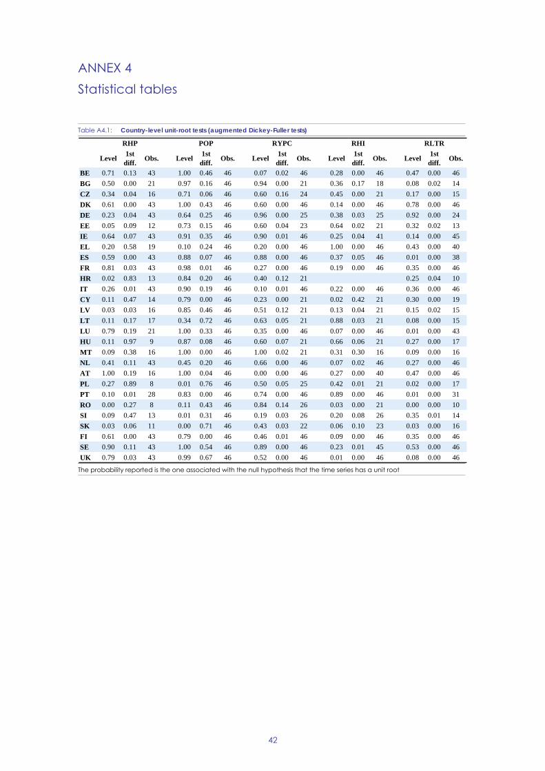

ISBN 978-92-79-64887-8
KC-BD-17-048-EN
-N