Assessing Ex Ante the Poverty and Distributional Impact of the Global

Crisis in a Developing Country

A Microsimulation Approach with Application to Bangladesh

Bilal Habib, Ambar Narayan, Sergio Olivieri and Carolina Sanchez-Paramo*

February 19, 2010

(Draft for comments: not to be cited or distributed without permission from authors)

Abstract

Measuring the poverty and distributional impact of the global crisis for developing countries is not

easy, given the multiple channels of impact and the limited availability of real-time data. Commonly-

used approaches are of limited use in addressing questions like who are being affected by the crisis

and by how much, and who are vulnerable to falling into poverty if the crisis deepens? This paper

develops a simple microsimulation method, modifying models from existing economic literature, to

measure the poverty and distributional impact of macroeconomic shocks by linking macro

projections with pre-crisis household data. The approach is then applied to Bangladesh to assess the

potential impact of the slowdown on poverty and income distribution across different groups and

regions. A validation exercise using past data from Bangladesh finds that the model generates

projections that compare well with actual estimates from household data. The results can inform

the design of crisis monitoring tools and policies in Bangladesh, and also illustrate the kind of

analysis that is possible in other developing countries with similar data availability.

Poverty Reduction and Equity Group, Poverty Reduction and Economic Management

World Bank, Washington DC

* This paper is the first in a series of country notes to be prepared under the work program on Analyzing the

Distributional Impact of the Financial Crisis, in the Poverty Reduction Group of the PREM Network. We gratefully acknowledge the data, inputs and comments received from the Bangladesh PREM Team of the World Bank – in particular Zahid Hussain, Sanjay Kathuria, Lalita Moorty, Nobuo Yoshida and Sanjana Zaman. We also thank the participants at a seminar organized in South Asia Region of the World Bank, Washington DC for their insightful comments on the interim results of this work.

1

1. Introduction

What began as a financial crisis in a few industrialized countries is quickly turning into a job crisis, with

contractions in growth taking their toll on developed and developing countries alike. The projected

economic slowdown across the world, recent World Bank global estimates for poverty suggest, could

add an extra 50 million to the number of people living below $1.25 a day and 64 million to the number

below $2 a day, compared to a scenario of uninterrupted growth in the absence of the crisis. By 2010,

the crisis is projected to add an estimated 89 million to the number of people living below $1.25 a day

and 120 million to the number below $2 a day (Chen and Ravallion, 2009). Along with the impact on

poverty numbers, the crisis is also likely to have significant impacts on the distribution of income and

consumption among the poor and nonpoor, both within and between countries.

Evidence from previous crises suggests that the output elasticity of wages tends to be larger during

downturns than during booms, and that relative inequality falls about as often as it rises during

aggregate contractions (Paci et al, 2008). Further, the crisis is rapidly shifting across countries – via

trade, financing, and remittances – as well as within countries – via adjustments in domestic credit and

labor markets and fiscal policies. As a result, it is difficult to predict the distributional impacts of the

crisis with a high degree of confidence.

There are some hypotheses about how the impact of the crisis is likely to evolve between different

groups in developing countries. The emerging consensus is that the initial impact is likely to be seen

mainly on the emerging middle-class, since they are more likely to be employed in export-oriented

industries and salaried jobs in the services sector, which appear to have suffered the largest labor

market shocks.1 Approximately 90% of households entering the middle-class during 1990-2005 joined

the lower tier ($2-9/day) (Ravallion, 2009), and thus risk falling back into poverty if they face large

employment or earnings shocks. The initial impact on the poor may be limited due to the very isolation

from the global markets (and the formal sector that gains the most from such linkages) in many

countries that have prevented them from exiting poverty in the past.

As the crisis unravels, however, the poor in developing countries are likely to be increasingly impacted.

With labor markets in the formal sector being affected, job opportunities and wages are likely to fall,

pushing more people into the informal sector, which could depress earnings in the informal sector. This

can be accompanied by reverse migration from urban to rural areas, increasing the burden on poor rural

households and drying up remittances from workers previously employed in the formal sector, leading

to higher and deeper poverty.

The distributional impact of the crisis is thus likely to be complex and dynamic. Some of the key

questions an analysis of distributional impacts would need to address are: how are the impacts going to

1 There is little consensus in the development literature about who the “middle class” are. A number of different

definitions have been used to study the evolution of the middle-class, such us Blackburn and Bloom (1987), Beach (1989), Levy and Murnane (1992), Jenkins (1995) and Burkhauser et. al (1999). For our purpose, we define the middle-class broadly, as those above the poverty line but below the richest decile (10%) of the population. In Bangladesh, this is the group between the 40

th and 90

th percentiles of per capita expenditure or income.

2

be shared across the distribution of income or consumption, which sectors, areas and regions are likely

to be impacted, and what are the characteristics of those who would become poor as a result of the

crisis? In order to be useful to policymakers in countries, these questions would have to be analyzed ex

ante, with available data that in most cases pre-date the crisis, rather than be delayed till the time post

(or during) crisis data become available. Even in cases where some real-time data is available from crisis-

affected sectors or countries, an ex ante approach can be useful to simulate future impacts for

hypothetical scenarios that are not available from real-time data, especially in countries where the

situation on the ground is changing rapidly.

Current approaches to analyze ex ante the impact of a macroeconomic shock, with the limited data

available in most countries, are somewhat inadequate in addressing the kind of questions posed above.

To improve upon existing approaches given the typical data constraints seen in most developing

countries, we develop in this paper a microsimulation model to evaluate ex-ante the distributional

impacts of the crisis. Section 2 outlines a rationale for building such a model, including the value added

from this approach compared to existing methods. Section 3 presents the model, starting with an

overview of the approach and subsequently outlining each step in detail, and ending with the key

limitations and caveats to the model. In Section 4, we discuss a country case study with an application of

our model (the case of Bangladesh). Section 5 concludes with implications of the results for Bangladesh

and possible areas for extension in the course of future work.

2. Rationale for our approach

Currently, there are two approaches commonly used within the World Bank to assess the welfare

(primarily consumption or income poverty) impacts of the crisis: the output elasticity of poverty

method, and PovStat (World Bank PovertyNet). The elasticity method involves using historical trends of

output and poverty to determine the responsiveness of poverty rates to growth in output (and

consumption), which is then combined with macroeconomic projections to estimate the impacts of

future reduced growth on poverty. Although this method is easy to implement and serves as a

convenient benchmark, it is limited in its predictive capability since it yields only aggregate poverty

impacts, with no account of the broader distributional effects. It may also prove deficient in predicting

poverty impacts during a crisis that affects output growth in a way not entirely consistent with the

recent growth experience in a country. This crisis, for example, is likely to impact some sectors more

than others and have a disproportionate impact on inflows like external remittances that directly impact

household income.

PovStat is an EXCEL-based World Bank simulation package, which uses household survey data and

macroeconomic projections as inputs and estimates changes in poverty and inequality indicators.

Although it allows for the impacts to occur through multiple channels, it offers no easy way to account

for changes in non-labor income (such as remittances), which has important implications in the context

of this crisis in some countries. By focusing exclusively on household heads (and ignoring the

employment status of other household members), PovStat also does not allow for a full accounting of

labor market impacts. Perhaps the most important limitation of PovStat is that it generates estimates for

poverty and inequality (aggregate or disaggregated by regions/groups) but not the kind of distributional

3

results that require individual or household level projections. For example, an important distributional

question like how the impact of the crisis is likely to be distributed across different groups

(differentiated by income status, sector, region or any other relevant attribute) cannot be answered

with PovStat.

More sophisticated simulation approaches than Povstat have been used in some cases by the World

Bank (see Bourguignon et al, 2008).2 All of them are based on a Computable General Equilibrium (CGE)

or General Equilibrium macroeconomic model that demand a lot of information (for constructing Social

Accounting Matrices or time-series of macroeconomic data) in order to create the “linkage aggregate

variables” (LAVS) that are fed into the microsimulation model. At the same time, these models do not

allow for changes in some key features of the population, such as gender or age composition, and the

economy (Ferreira et al, 2008). The main advantages of these models are related to improved accuracy

of the counterfactual and consistency of the analysis. Notably, the information demands of these

models make them hard to apply in most developing countries, and calls for an approach that is

workable with available data and macroeconomic projections.

Because the nature of the crisis is difficult to pin down, any valid impact assessment needs to account

for multiple transmission mechanisms and capture impacts at the micro level over the entire income

distribution. In the microsimulation model presented here, we do this by focusing on labor market

adjustments in employment and earnings, non-labor income, and price changes (with a view to the

variation in food/non-food prices). Note that for the purposes of this exercise, we use the terms “labor

income” and “earnings” interchangeably.3

Our proposed methodology can be seen as a compromise between the “simple” methodologies like

PovStat and the “complex” ones using general equilibrium models – with the attendant advantages and

disadvantages. Compared against the simpler approaches, the value added by our approach is two-fold.

First, the model is able to generate estimates for individuals and households across the distribution with

and without the crisis, which can be used for detailed poverty and distributional analyses of impact.

Second, the model uses income rather than consumption; this allows us to model labor and non-labor

incomes separately, which is particularly important for countries in which remittances and public

transfers form a large proportion of incomes.

In comparing our approach with PovStat, the pros and cons of either method should be kept in

perspective. Our model in its most basic form has data requirements similar to that for PovStat, and

adds value along the two important dimensions stated above. At the same time, it requires considerably

more computational resources and time than PovStat, which can be run as a simple Excel-based model

once the household and macroeconomic data are ready to be fed into the model. Compared with the

complex approaches, the primary advantage of our approach is the lower demand for information,

2 These include the micro accounting approach (Computable General Equilibrium-Representative Household

Groups), top-down micro simulations models (CGE-Micro or Macro models) and Feedback loops from bottom-top (Bourguignon et. al 2008). 3 In fact, “labor income” is defined here as the total income earned from any sort of labor activity by all members

of a household, including wages and profits.

4

which would make it practical to apply in many cases where the more complex approaches would have

to be ruled out.

3. Proposed approach

We propose to use a microsimulation model that combines macroeconomic projections with pre-crisis

micro data from household and/or labor force surveys to predict income and consumption at the

individual and household level under different scenarios, which can then be compared to measure

poverty and distributional impacts. Comparisons will be made between different projected scenarios

(most commonly a crisis or low scenario and a benchmark or base scenario) rather than a time

comparison (i.e. a comparison between 2005 and 2009 or 2010 in the case of Bangladesh). Figure 1

presents a stylized representation of the methodology.

The model focuses on labor markets and

migration as transmission mechanisms and

allows for two types of shocks: shocks to labor

income, modeled as employment shocks,

earnings shocks or a combination of both; and

shocks to non-labor income, modeled as a shock

to remittances. Shocks can be positive or

negative depending on the trends outlined by

the macroeconomic projections. In most cases

labor income and remittances account for at

least 75-80% of household income. Minimum

assumptions are made about other sources,

such as capital and financial income or public

transfers, as discussed below.

The data requirements can be summarized as follows. At the macro level, information is needed on

projected (i) output, employment, remittances and (ideally) labor earnings growth; (ii) population

growth and (iii) predicted price changes. At the micro level, information is needed on (i) labor and non-

labor income and consumption, and (ii) labor force status and basic job characteristics, including

earnings. Needless to say, the reliability and accuracy of the simulation results is a direct function of the

quality and level of detail of the information available at the macro and micro levels.

Finally, the income and consumption projections from the model can be used to produce a variety of

outputs, including aggregate poverty and inequality comparisons across scenarios, poverty and

vulnerability profiling of specific groups and/or areas, and various summary measures of distributional

impacts, such as growth incidence curves and state transition matrices. We comment on these

extensively for the case of Bangladesh below.

Figure 1: Microsimulation methodology

5

3.1 Overview of simulation exercise

In this Section we provide a brief overview of the mechanics underpinning the simulation exercise. The

exercise can be broken down into three distinct steps: calibration, simulation and assessment of

impacts. A description of each step follows and a schematic of the complete model is presented in

Figure 2.

Figure 2: Schematic of the microsimulation model

Calibration. Calibration is the process by which household and individual-level information is used to

model labor market behavior and outcomes and to predict the likelihood of receiving remittances.4 This

is done in three steps. First, we model labor force status for all working age individuals (15-64) as a

function of household and individual characteristics, where labor force status can be non-employed,5

employed in agriculture, industry or services. Although ideally we would like to work with a more

detailed menu of options (e.g. “employed in tradeables” and “employed in non-tradeables” instead of

“employed in industry”), the number of labor force states that can be considered is dictated by the level

of disaggregation available for the macro projections. We then use a multinomial logit to estimate the

parameters of the model, as well as the individual-level probability of remaining in a particular state

and/or changing to a different one, as given by (1). The approach is similar to that used in Ferreira et al

(2009). We estimate the model separately for high and low-skill individuals to allow for structural

differences in the labor market behavior of the two groups.6

4 We estimate a reduced form of the household income-generation model which is based on Bourguignon and

Ferreira (2005) and Alatas and Bourguignon (2005) 5 This includes “out of the labor force” and “unemployed”. The decision to pool both states into a single category is

motivated by the fact that the unemployment rate is extremely low in Bangladesh, even during crisis times. 6 For Bangladesh, low and high-skilled refer to individuals with 0 – 9 and >10 years of education, respectively.

6

(1)

where s = Labor force status; G = labor skill level (high/low); z = gender, age, education, region, remittances, and

land ownership.

Second, we model labor earnings for all employed individuals ages 15 to 64 as a function of individual

and job characteristics and use a standard Mincerian OLS regression to estimate the parameters of the

model, as given by (2) (similar to Ferreira et al. 2008). We use a fairly broad definition of labor earnings

for the purpose of the exercise that includes wages and salaries, but also income from self-employment.

This is particularly important in the case of agriculture and for economies with large informal sectors,

such as Bangladesh, since wage and salaried workers constitute a limited fraction of those employed in

these sectors. It may lead however to a loss in precision and/or predictive power given that the

structural relationship between individual and job characteristics and earnings could be different for

salaried and non-salaried workers. To allow for maximum flexibility and (indirectly) account for some of

these differences we estimate the model separately for agriculture, industry and services and for low

and high-skill workers.7

(2)

where x =gender, age, education, region, land ownership, and indicators for export industry, salaried and public

employment.

The results of the estimation of equations (1) and (2) and a full description of all variables can be found

in Annex 1.

Finally, we model non-labor income with a focus on international remittances and make some minimal

assumptions about other sources of non-labor income. Ideally, we would estimate a probit model to

estimate the probability of how likely a household would be to receive international remittances, given

its characteristics. However, if the migration-related information in the survey is poor or insufficient

and/or the predictive power of probability model is low (as is the case for Bangladesh), we are better-off

relying on a simple non-parametric assignment rule that is consistent with the existing evidence (the

specific rule used for Bangladesh is discussed in more detail when we describe the simulation process).

Simulation. Simulation is the process by which information on aggregate projected changes in output,

employment and remittances is used to generate changes in labor and non-labor income at the micro

level using the structural models developed as part of the calibration.8 This is done in four steps.9 First,

7 Notice that, although we could estimate separate models for salaried and non-salaried workers based on the

information from the household survey, we would not be able to use these models for the purpose of predicting future earnings since we do not have earnings and employment information disaggregated by salaried/non-salaried workers from macro data. 8 We do not assure consistency (i.e that absolute aggregate magnitudes are equal) between the data set used at

the two modeling stages (see Bourguignon et. al 2008). Additionally, we assume equal changes at macro and micro levels. We cannot run a test if macro changes are similar or not to micro changes because of lack of a panel data at micro level (see Deaton 2001 and Bourguignon et al 2008). 9 This sequence for introducing changes in the model is based on Vos et al (2002)

G

is

G

si

G

s

G

i vxw ,log

sjubzaubzaIndI j

i

j

i

js

i

s

i

sG

sji |,

7

we use population growth projections to adjust for demographic changes between 2005 (base year) and

2009-2010. This adjustment is particularly important in the case of Bangladesh because fertility rates are

still high, which implies that the number of labor market entrants rises faster than overall population,

and the baseline household survey is relatively old. In practical terms, taking into account population

growth allows us to explicitly take into changes in the size of the working age population, and hence to

distinguish between employment growth driven (or rather absorbed) by demographic trends and net (or

additional) employment growth.

Secondly, we use the projections from the labor force status and labor earnings models to replicate

projected changes in aggregate total and sectoral output and employment. We start with employment

and calculate the total number of individuals that need to be reassigned between employment and non-

employment and across employment sectors in order to match projected aggregate changes in total and

sectoral employment. We then use the estimated probabilities from the multinomial model to select

candidates for reassignment.10 The direction and magnitude of flows between employment and non-

employment and across sectors of employment is given by changes in the relative shares of different

status with respect to the reference population. For instance, whether individuals must be reassigned

from non-employment to employment or vice-versa depends on whether the employment rate of

individuals ages 15 to 64 is increasing or decreasing. Similarly, workers are expelled from sectors whose

relative share in total employment is declining and absorbed into sectors whose relative share in total

employment is increasing will absorb workers (note that this is independent of whether employment in

a sector is growing or contracting in absolute terms).

The sequence in which individuals are reassigned across states and sectors matters for the final

simulation results so we briefly describe here the procedure we follow:

Step 1 - Flows between employment and non-employment: If the employment rate is

increasing, non-employed individuals with the lowest predicted probability of being non-

employed will be reassigned. If the employment rate is declining, employed individuals with the

highest probability of being non-employed will be reassigned. Reassignments will continue up to

the point where the change in the employment rate at the micro level matches the change at

the macro level.

Step 2 - Flows out of contracting sectors: For sectors whose share of total employment is

declining, those individuals with the lowest predicted probability of being employed in the

sector will be selected out and added to the pool of “eligible” workers to be employed in

growing sectors (notice this pool also contains those who has been reassigned from non-

employment if the total employment rate is growing). Reassignments out of each sector will

continue up to the point where the change in the sector employment share at the micro level

matches the change at the macro level.

10

We add error terms which represent the unobserved heterogeneity of agents’ labor supply behavior. These lead to some disparateness in responses to a change in the labor demand, capturing the fact that in the real world individuals who are identical in observables might still respond differently the same change in labor demand.

8

Step 3 – Flows into growing sectors: Individuals in the pool of “eligible” workers will be assigned

to growing sectors on the basis of their predicted probability of being employed in each sector.

Assignments are made sequentially with the sector whose employment share is growing fastest

absorbing workers first and the sector whose employment share is growing the slowest

absorbing workers last. Reassignments to each sector will continue up to the point where the

change in the sector employment share at the micro level matches the change at the macro

level.

There are a few important features of this process that are worth mentioning. The reassignments

described in steps 1 to 3 are calibrated so as to replicate net aggregate flows between employment and

non-employment and across sectors. In reality, movements across these different states are quite

significant so that gross flows are usually larger than net flows. The order of proposed steps is such that

it allows for non-employed individuals to become employed and employed individuals to become non-

employed, but also for individuals to change sectors. In doing this we try to capture the fact that highly

“employable” individuals are more likely to remain employed in one sector or another, at times at the

expense of less “employable” workers (i.e. highly “employable” workers will crowd others out when

employment opportunities become relatively more scarce).

We next use the earnings model estimated as part of the calibration to predict earnings for two groups

of workers: those with no previous earning history (i.e. non-employed in 2005) and those who change

sector of employment. Because earnings are a function of both observable and unobservable individual

and job characteristics, we add a random element to the predicted earnings produced by the model to

account for unobserved heterogeneity.11 For all other individuals, we use the earnings information

available in the household survey.

Once all workers have been assigned positive labor earnings, total earnings in a sector are adjusted to

match aggregate projected changes in output. This step relies on the fact that that projected changes in

sectoral output can be explained by projected changes in sectoral employment and projected changes in

sectoral earnings and profits, and assumes that earnings and profits grow at the same rate.

The treatment of public sector workers and those with more than one job differs slightly from what we

just described. Total public sector employment is assumed to remain constant (i.e. no individuals are

assigned to or out of the public sector) and labor earnings of public sector workers are adjusted in line

with their sectoral mapping (agriculture, industry or services). Similarly for those holding more than one

job, we assume the sector of employment of their secondary activity remains constant while earnings

are adjusted in line with sectoral changes.

The third step in the simulation process pertains to changes in international remittances. As mentioned

above, in the case of Bangladesh we simulate these changes following a very simple allocation rule. We

calculate the total change in international remittances between 2005 and 2009-2010,12 using actual and

11

Specifically, we draw an individual error from the error distribution generated during the estimation. 12

The nominal (in dollar terms) growth in external remittances is adjusted using the taka/$ exchange rates of the relevant years, to arrive at the value of change in remittances in constant 2005 takas.

9

projected data (this change is positive under both the crisis and the benchmark scenarios) and allocate

the dividend as follows: (i) across divisions, remittances are allocated proportionally to the 2005 across-

division distribution; (ii) among households within divisions: recipient households are selected at

random and given a remittance transfer equivalent in real terms to the median remittance transfer in

that division in 2005, with the number of total transfers to be made within each division being equal to

the total amount of additional remittances to be distributed divided by the 2005 median value.13 As a

result of this process the overall distribution of remittances across divisions remains unchanged; while

there is an increase in number of recipient households (both types of households, those who did or did

not receive remittances in 2005, can receive new remittances in 2009-10).

Finally we simulate changes in other sources of non-labor income. For this we assume that capital and

financial income grow at the same rate as real GDP, public transfers (primarily Social Security transfers)

remain constant in real terms at 2005 levels, and domestic remittances change at the same rate as labor

income. These assumptions appear to be reasonable for Bangladesh, and can be modified for other

countries depending on country circumstances.

Assessment of Impacts. Impact assessment is the process by which we use the information on individual

employment status and labor income, as well as on non-labor income at the household level, to

generate income and consumption distributions and construct various poverty and distributional

measures that can then be used to compare the crisis and the benchmark scenarios. This is done in

three steps.

First, we account for the fact that between 2005 and 2009-2010, food prices have increased at a higher

rate than other prices. To ensure that the same food basket is affordable at the new prices, we adjust

the 2005 poverty line to reflect the increase in food prices relative to that of other prices (for more

details, see Section 4.4 below) 14.

Second, we calculate total household income by aggregating labor income across all employed

individuals and adding non-labor income, and then use information on household size to construct a

measure of per-capita household income, as in (3).

(3)

Third, because poverty in Bangladesh is measured on the basis of per-capita consumption, we need to

map income to consumption. We do this by assuming that the household-level consumption-to-income

13

To illustrate, 23% of additional remittances are allocated to rural Dhaka, equal to its share of remittances in 2005. Every randomly selected recipient household then receives 5,417 taka/month, equivalent to the median international remittance transfer in the division in 2005 (<U$ 90 dollars per month with an exchange rate of tk.61/U$S) 14

An alternative, more sophisticated way of dealing with this problem would be to construct household-specific consumption deflators that take into account differences in consumption patterns across the income/consumption distribution.

m

NL

m

k

i

ii

mk

yIw

PCI

m

*

1

**

*

10

ratio remains unchanged between 2005 and 2010. This is a strong assumption, but the best we can do

given the available information. We may try to refine this step in future iterations of the exercise.

(4)

Finally, we use information on household and individual income and consumption levels to evaluate the

poverty and distributional impacts of the crisis by comparing poverty and other outcomes between the

benchmark (without crisis) and “with crisis” scenarios.

3.2 Limitations and caveats of the simulation exercise

The proposed approach has some appealing features, the primary one being its capacity to generate

income and consumption counterfactuals at the individual and household levels that can then be used

to assess impacts across the entire distribution. However, it also has some important limitations that

must be taken into account when interpreting the results presented below. We discuss these below.

Firstly, the quality and accuracy of the simulation output is a function of the nature and quality of data

underpinning the exercise. More specifically, the results would depend not only on the micro-models,

but also on the macro projections of the crisis and the benchmark or no-crisis scenarios. In a typical ex-

ante assessment of this type, building the counterfactual to evaluate impact is especially tricky because

the comparison between the situations “with” and “without” the “treatment” (the macro shock) is

purely virtual or notional. This is particularly important with regard to the output and employment

projections since they are key drivers of the results in the absence of a CGE or similar model. In addition:

The ability to account for heterogeneity across sectors, groups, and others depends on the level

of disaggregation of the available macro projection. For instance, the behavior of the tradeable

and non-tradeable sectors within industry can only be modeled separately if output growth

projections are available for each sector.

The ability to accurately predict employment and earning changes depends on the available

information and on the assumptions needed to correct for information gaps. For instance, in the

absence of projections on total and sectoral earnings growth, we need to assume that earnings

and profits grow at same rate within a sector. How realistic this assumption is would depend on

the country and sectoral context.

The ability to model remittances depends on the quantity and quality of the available data on

migrants and remittances, particularly for countries with rapid and/or volatile growth of

remittances.

Secondly, the simulations implicitly assume that the structural relationships estimated as part of the

calibration process on the baseline data continue to be valid in the future years for which the

projections are made. The more distant in the past the baseline year is, the more questionable this

assumption is likely to be. In the case of Bangladesh, for example, the baseline year is 2005, which is a

full four to five years away from the prediction years (2009 and 2010). This particular caveat, however,

2005

2005** *

m

mmm

PCI

PCExpPCIPCExp

11

links directly back to the constraints imposed by availability of data. In most countries, household survey

data that is available for analysis and processed to the extent necessary for the analysis is likely to pre-

date the prediction years (usually 2010) by at least 3 to 4 years.

The third caveat relates to our decision to work with income, rather than consumption data. The

advantage of using income is that it allows us to link welfare impact on households directly with

potential channels of impact, which are employment, labor earnings and remittances. There are two

primary caveats to working with income data: (i) income data often tends to be of lower quality than

consumption data, which introduces an element of noise into the analysis due to the unobserved

presence of measurement error; (ii) certain assumptions, which can be challenged on the grounds of

realism, are needed to convert predicted income levels into consumption and consumption-based

welfare measures. It is important to note, however, that (ii) would not be necessary for countries that

use an income-based measure of poverty, which is the case in most Latin American countries.

The approach we have adopted to convert income into consumption assumes that the ratio of

consumption to income is unchanged for every household between the baseline and prediction years.

The constant savings rate that this assumption implies is probably more realistic for poor households

than for better-off households. This also implies that our approach may overestimate the consumption

impact of the crisis on better-off households, since such households may compensate for an income loss

by reducing savings (or dis-saving), resulting in a smaller impact on consumption.

Fourthly, our model does not explicitly account for labor demand at the sectoral level and instead

assumes that the labor market conditions mirror (or are proxied by) the macroeconomic projections.

The simple approach we adopt implicitly assumes stable relationships between output, demand for

labor and labor earnings, which may not hold due to the distortions (such as segmentation and

downward stickiness of nominal wages) that typically exist in the labor market and are likely to affect

adjustments during a crisis.

Related to the above point, the simplifying assumptions for the labor market also do not account for the

possibility of structural shifts in labor demand due to the crisis. Sectoral movements of labor are

modeled as depending only on individual/household characteristics (through the multinomial logit

model) and population growth. This cannot take into account the kind of structural shifts that have

apparently been observed in some countries, such as a reduction in the relative demand for skilled

labor. That said, structural changes (for example, in relative demand for skills) can be incorporated into

our model if there exists prior analytical work that provides parametric estimates of how these changes

may have affected labor earnings.

Fifthly, our model is limited in its ability to account for shifts in relative prices between different sectors

of the economy as a result of the shock. The model does take into account the impact of shifts in the

price of food relative to general inflation on poverty measures, by using the simple device of adjusting

poverty lines that are anchored to a fixed food basket. It can be argued that changes in the relative price

of food represent the most significant source of price impact on poor or near-poor households in a

country like Bangladesh, as the recent food crisis has shown. At the same time, there are other potential

12

sources of price impacts – for example, the effect of a change in the terms of trade between agriculture

and other sectors on real household incomes in all sectors – our approach does not take into account.

Unfortunately, in the absence of a CGE model to link up to, it is nearly impossible to explicitly model for

changes in terms of trade between sectors.

The final limitation, related to validation of hypothesis, applies to all ex-ante approaches including ours.

The only validation or test for our simulation model is to combine ex-ante and ex-post analysis (see

Bourguignon and Ferreira, 2003). Since ex post data will not be available for some time, some

uncertainty about the validity of the simulations generated by this ex-ante method is bound to remain.

4. The Bangladesh case study

Bangladesh is a good case study for our model for a number of reasons. Most importantly, it is a low-

income, high-growth country with an export sector that is significant but not predominant. As a result,

its exposure to the direct impact of the crisis is on the moderate to low side, which is typical of a

majority of developing countries. The relatively low exposure also makes it possible to see how the

model predicts the impact of relatively small shocks to the economy and how sensitive the results are to

changes in macroeconomic projections and assumptions. Bangladesh also has a reasonably balanced

economy, with all three principal sectors contributing positively to GDP growth. The importance of

agriculture has been declining gradually over the last 15 or so years (Paci and Sasin 2008), similar to

what is seen for most developing countries. In sum, Bangladesh appears to have many of the features

that are typical to a developing country. It is also an important country from a global poverty

perspective, given its relatively high poverty rate and large population, which translate to a large

number of poor people.

In terms of data availability, Bangladesh measures up quite well to most low-income countries. A fairly

recent household survey is available (Household Income and Expenditure Survey/HIES of 2005), which is

the latest in a long series of surveys that have been used to track poverty and related estimates. The

availability of a recent Poverty Assessment report, based primarily on HIES 2000 and 2005, is an added

plus since it provides information on poverty and labor market that can inform the specifications of our

empirical models. The available macroeconomic information is however limited, with disaggregated

output growth projections available at the sectoral level but not for key sub-sectors. Moreover, while

the household survey is detailed enough to apply our model, the base year (2005) is far enough from the

target years for projections (2009 and 2010) that we cannot rule out structural changes not captured by

our model.

4.1 Background: poverty reduction in Bangladesh15

Growth and Poverty in Bangladesh. Bangladesh has enjoyed a fairly stable macroeconomic

environment with high growth and significant poverty reduction over the past 15 years. Poverty

headcount rate declined from 57% in the early 1990s to 49% in 2000 and 40% in 2005. The rate of

15

The discussion in this sub-section is based on findings from World Bank (2007, 2008) and Paci and Sasin (2009). All figures cited are from World Bank (2008).

13

reduction during 2000-2005 was one of the highest in South Asia region for comparable periods. Poverty

reduction was driven by robust GDP growth, which averaged above 5% annually during 2000-05, along

with stable relative inequality (the Gini of per capita consumption remained unchanged at 0.31 since

mid-1990s). While all sectors – agriculture, industry and services – are expanding, agricultural growth

has been lagging behind that of other sectors, with the result that the contribution of agriculture to GDP

fell from around 30% in the beginning of 1990s to just above 20% in 2005.

Poverty reduction and the labor market. Poverty reduction between 2000 and 2005 was linked to

significant transformations in the labor market and rapid increases in remittances. Economic growth,

driven mainly by factor accumulation in the private sector and rapid growth of the export sector, led to

wage growth and enhanced labor productivity. Between 2000 and 2005, the share of agriculture in total

employment declined – agricultural employment grew at 0.7 percent per year compared to 5 and 2.8

percent for services and manufacturing respectively. There was a movement away from low productivity

jobs in agriculture to more productive jobs in the nonfarm private sector, particularly in urban areas.

These trends are consistent with the shrinking share of agriculture in GDP while the share of services

and industry was increasing.

Increasing flow of remittances (20% growth annually during 2000-2005) was another key factor

contributing to poverty reduction.16 Government statistics on documented migration estimate that

more than 3.7 million Bangladeshi have emigrated during the past 30 years and about 3 million – or 6%

of the in-country economically active population – were estimated to be living abroad in 2005.

Notwithstanding the progress, however, Bangladesh had an estimated 56 million people in poverty in

2005 and wide disparities across income and occupational groups, gender, and regions. Poverty was

most prevalent among daily agricultural wage workers and subsistence farmers while the better-off

tended to be engaged in salaried employment or nonfarm self-employment. The likelihood of poverty

was also higher when a household had a larger number of dependents and low levels of education, and

did not receive remittances. The poverty rate in 2005 among households receiving remittances from

abroad was 17% compared to 42% among the rest.

Regional differences in poverty reduction. Underlying the national poverty story were vast differences

between regions. Dhaka, Chittagong, and Sylhet divisions in the eastern part of the country experienced

rapid poverty reduction between 2000 and 2005. Dhaka and Chittagong divisions, with just over half the

country’s population in 2000, contributed nearly 80% of the reduction in national poverty during this

period. In the West, meanwhile, gains were much smaller for Rajshahi and nonexistent for Barisal and

Khulna. As a result, in 2005, the poverty rate was between 30% and 35% in Dhaka, Chittagong and Sylhet

divisions, and more than 45% in Khulna, Barisal and Rajshahi (more than 50% in Barisal and Rajshahi).

16

Equally important were some of the forces that have emerged from social transformations occurring over time. A fall in the number of dependents in a household, linked to past reductions in fertility, has been an important contributor in raising per capita incomes, as has been increases in labor force participation and educational attainment, particularly among women.

14

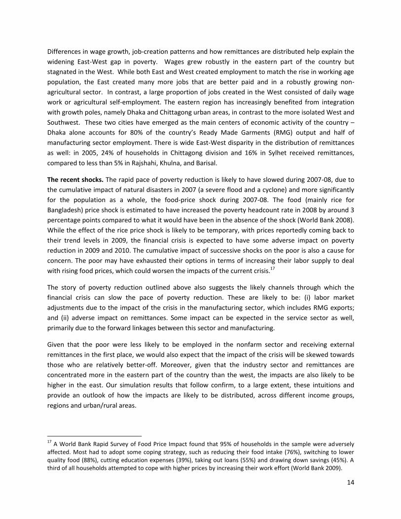
Differences in wage growth, job-creation patterns and how remittances are distributed help explain the

widening East-West gap in poverty. Wages grew robustly in the eastern part of the country but

stagnated in the West. While both East and West created employment to match the rise in working age

population, the East created many more jobs that are better paid and in a robustly growing non-

agricultural sector. In contrast, a large proportion of jobs created in the West consisted of daily wage

work or agricultural self-employment. The eastern region has increasingly benefited from integration

with growth poles, namely Dhaka and Chittagong urban areas, in contrast to the more isolated West and

Southwest. These two cities have emerged as the main centers of economic activity of the country –

Dhaka alone accounts for 80% of the country’s Ready Made Garments (RMG) output and half of

manufacturing sector employment. There is wide East-West disparity in the distribution of remittances

as well: in 2005, 24% of households in Chittagong division and 16% in Sylhet received remittances,

compared to less than 5% in Rajshahi, Khulna, and Barisal.

The recent shocks. The rapid pace of poverty reduction is likely to have slowed during 2007-08, due to

the cumulative impact of natural disasters in 2007 (a severe flood and a cyclone) and more significantly

for the population as a whole, the food-price shock during 2007-08. The food (mainly rice for

Bangladesh) price shock is estimated to have increased the poverty headcount rate in 2008 by around 3

percentage points compared to what it would have been in the absence of the shock (World Bank 2008).

While the effect of the rice price shock is likely to be temporary, with prices reportedly coming back to

their trend levels in 2009, the financial crisis is expected to have some adverse impact on poverty

reduction in 2009 and 2010. The cumulative impact of successive shocks on the poor is also a cause for

concern. The poor may have exhausted their options in terms of increasing their labor supply to deal

with rising food prices, which could worsen the impacts of the current crisis.17

The story of poverty reduction outlined above also suggests the likely channels through which the

financial crisis can slow the pace of poverty reduction. These are likely to be: (i) labor market

adjustments due to the impact of the crisis in the manufacturing sector, which includes RMG exports;

and (ii) adverse impact on remittances. Some impact can be expected in the service sector as well,

primarily due to the forward linkages between this sector and manufacturing.

Given that the poor were less likely to be employed in the nonfarm sector and receiving external

remittances in the first place, we would also expect that the impact of the crisis will be skewed towards

those who are relatively better-off. Moreover, given that the industry sector and remittances are

concentrated more in the eastern part of the country than the west, the impacts are also likely to be

higher in the east. Our simulation results that follow confirm, to a large extent, these intuitions and

provide an outlook of how the impacts are likely to be distributed, across different income groups,

regions and urban/rural areas.

17

A World Bank Rapid Survey of Food Price Impact found that 95% of households in the sample were adversely affected. Most had to adopt some coping strategy, such as reducing their food intake (76%), switching to lower quality food (88%), cutting education expenses (39%), taking out loans (55%) and drawing down savings (45%). A third of all households attempted to cope with higher prices by increasing their work effort (World Bank 2009).

15

4.2 Macroeconomic projections of crisis impact

Projections of aggregate and sector-specific growth rates for 2009 and 2010, obtained from the World

Bank Bangladesh country office, are used as inputs into our microsimulation model (see Annex 2, Table

A.2 for more detailed data). In conducting simulations, two scenarios are considered for each year: (i)

the scenario with crisis, and (ii) the benchmark or “no-crisis” scenario (namely projections that were

made before the crisis hit).

Aggregate GDP growth is expected to be 0.8 and 1.5 percentage points lower with crisis compared to

the benchmark or no-crisis

scenario, in 2009 and 2010

respectively (Table 1). Growth of

output in industry and services is

projected to slow down by 1.1 and

1.2 percentage points respectively

in 2009 and by 3.3 and 1

percentage points respectively in

2010. The impact is most

significant in the industry sector

primarily due to a fall in demand

for manufacturing exports and the

spillover effect this may have on

ancillary industries. The impact is

much smaller for the service sector

since services in Bangladesh are

generally not traded and therefore less susceptible to global trends.

Importantly, remittances are expected to be lower by about 10% due to the crisis in 2010, compared to

the no-crisis scenario. In 2009 however, the available figures suggest that the actual growth in

remittances in 2009 was about the same as it was predicted before the crisis. Even with the crisis,

remittances are expected to grow by 12% between 2009 and 2010 in dollar terms, which is however

quite a bit lower than the 21% growth that was expected had there been no crisis.

In sum, the macroeconomic impacts of the crisis, according to the latest projections, are estimated to be

relatively small in Bangladesh and occur mainly in the industry sector and remittances. This suggests

that the impact on labor earnings of household is likely to be small in both 2009 and 2010 and skewed

towards households earning income from industry sector. The adverse impact on remittance growth

would lead to some losses in household non-labor income for year 2010, but not for year 2009.

18

For the purposes of the simulation, the remittance projections are converted into Takas using the taka:US$ exchange rate for each year, and then adjusted to 2005 takas using each year’s CPI (adjusted to base year 2005). In other words, the following formula is applied to each year’s remittance projection: R

R= R

N. ε/CPI, where R

R is the

amount in real takas (at 2005 prices), RN is the amount in nominal US dollars, and ε is that year’s exchange rate.

Table 1: Macroeconomic projections

Baseline With Crisis Impact of Crisis

(Crisis – Benchmark)

2005 2009 2010 2009 2010

Output growth (%)

Total GDP 5.9 5.8 5.6 -0.8 -1.5

Agriculture 2.2 4.6 3.6 0.6 -0.3

Industry 8.3 5.9 6.0 -1.1 -3.3

Services 6.4 6.3 6.1 -1.2 -1.0

Remittances (US$ millions)

18 3,848 9,689 10,872 -311 -1,228

Source: World Bank Bangladesh country office (as of September 2009)

Note: 1) Benchmark projections are the projections made for the relevant years at a time before the financial crisis occurred. 2) Crisis projections take into account the impact of the crisis.

16

4.3 Labor market projections and impact of crisis

Labor market status in 2005. In 2005 (according to HIES

data), about 48% of the working-age (15-64 years of

age) population was employed.19 Among those

employed, 44% was employed in agriculture, 24% in

industry, and 32% in services. 55% of those employed

were salaried workers, and 75% of the labor force had

less than 10 years of education (defined as “low-

skilled”). The employed population includes those

working for wages/salaries, the self-employed and

those contributing labor to household-based

enterprises or activities that produce income for the

household. On average, 68% of household income

comes from labor earnings and 9% comes from

remittances (from abroad and domestic), which in turn

constitutes about 39% of non-labor income (see Annex 2, Table B for detailed figures).

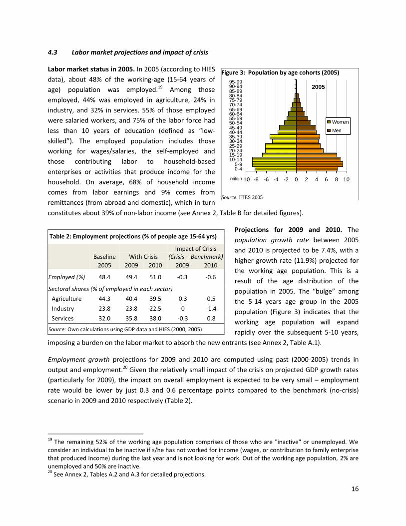
Projections for 2009 and 2010. The

population growth rate between 2005

and 2010 is projected to be 7.4%, with a

higher growth rate (11.9%) projected for

the working age population. This is a

result of the age distribution of the

population in 2005. The “bulge” among

the 5-14 years age group in the 2005

population (Figure 3) indicates that the

working age population will expand

rapidly over the subsequent 5-10 years,

imposing a burden on the labor market to absorb the new entrants (see Annex 2, Table A.1).

Employment growth projections for 2009 and 2010 are computed using past (2000-2005) trends in

output and employment.20 Given the relatively small impact of the crisis on projected GDP growth rates

(particularly for 2009), the impact on overall employment is expected to be very small – employment

rate would be lower by just 0.3 and 0.6 percentage points compared to the benchmark (no-crisis)

scenario in 2009 and 2010 respectively (Table 2).

19

The remaining 52% of the working age population comprises of those who are "inactive" or unemployed. We consider an individual to be inactive if s/he has not worked for income (wages, or contribution to family enterprise that produced income) during the last year and is not looking for work. Out of the working age population, 2% are unemployed and 50% are inactive. 20

See Annex 2, Tables A.2 and A.3 for detailed projections.

Figure 3: Population by age cohorts (2005)

Source: HIES 2005

Table 2: Employment projections (% of people age 15-64 yrs)

Baseline With Crisis Impact of Crisis

(Crisis – Benchmark)

2005 2009 2010 2009 2010

Employed (%) 48.4 49.4 51.0 -0.3 -0.6

Sectoral shares (% of employed in each sector)

Agriculture 44.3 40.4 39.5 0.3 0.5

Industry 23.8 23.8 22.5 0 -1.4

Services 32.0 35.8 38.0 -0.3 0.8

Source: Own calculations using GDP data and HIES (2000, 2005)

2005

-10 -8 -6 -4 -2 0 2 4 6 8 10

0-45-9

10-1415-1920-2425-2930-3435-3940-4445-4950-5455-5960-6465-6970-7475-7980-8485-8990-9495-99

milion

Women

Men

17

The impact on sectoral shares in employment is more significant, since the crisis does not affect all

sectors equally. In 2010, the share of industry in total employment is projected to be lower in the crisis

scenario by 1.4 percentage points, while those of services and agriculture are expected to be 0.8 and 0.5

percentage points higher, respectively (Table 2).

4.4 Impact on household income, poverty and distribution: results from microsimulation

It is important to note that the results of the simulation exercise are entirely dependent on the

macroeconomic projections (in Section 4.2 above), which can change as more information becomes

available. If the actual impact of the crisis on remittance growth in 2010, for example, were to be less

than the projections shown in Table 1, the impact on poverty and household incomes will also be lower

than what is estimated here. The primary purpose of this exercise should therefore be seen not as an

attempt to definitively predict future poverty in the highly uncertain environment of a global economic

crisis, but rather as illustrating the kinds of results and insights this simulation model can yield, given the

most recently available projections of macroeconomic impact of the crisis.

Average household income is expected to be 0.7% lower in 2009 and 2.4% lower in 2010 as a result of

the crisis (compared to the benchmark case), applying the microsimulation method described in Section

3. The drop in 2009 income is attributed to a 0.5% drop in labor income and 1.5% drop in non-labor

income, while in 2010 labor and non-labor income is projected to drop by 1.5% and 5% respectively. The

significantly higher loss in non-labor income in 2010 is due to a 9% loss in remittances in 2010 compared

to 3% in 2009 (see Annex 2, Table B for the detailed estimates on household income).

Impact on poverty and inequality. As expected, and consistent with the impacts on household income,

the impact of the crisis on poverty measures is low in 2009 and more significant in 2010. Table 3 shows

the projections for poverty and inequality measures for 2009 and 2010 with crisis and the projected

impact of the crisis for each year

(i.e. the difference between crisis

and benchmark scenarios).

The poverty headcount rate

(based on the upper poverty line)

and extreme poverty rate (based

on the lower poverty line) are

expected to be 0.4 and 0.2

percentage points higher in 2009,

respectively, as a result of the

crisis. In 2010, the poverty

headcount rate is expected to be

1.2 percentage points higher and

the extreme poverty rate 0.9

percentage points higher due to

the crisis. The impacts on poverty gap (depth of poverty) and squared poverty gap (severity) are small

Table 3: Impact of financial crisis on poverty and inequality indices

Baseline With Crisis

Impact of Crisis (Crisis – Benchmark)

2005 2009 2010

2009 2010

Moderate poverty -Headcount rate (%) 40.0 28.6 25.8

0.4 1.2

-Poverty gap 9.0 6.0 5.3

0.1 0.3

- Squared poverty gap 2.9 1.9 1.6

0.1 0.1

Extreme poverty

-Headcount rate (%) 25.1 16.7 14.8

0.2 0.9

-Poverty gap 4.7 3.0 2.5

0.1 0.1

- Squared poverty gap 1.3 0.8 0.7

0 0.1

Inequality per-cap. Exp -Gini 0.31 0.34 0.32

0.02 0

-Theil 0.19 0.22 0.19

0.02 -0.01

Source: Microsimulations using macro projections (see Table 1) and HIES (2005)

18

for both years, but slightly higher for 2010 than 2009. The impact of the crisis on aggregate measures of

inequality is negligible (see Annex 2, Table D.1 for detailed results).

The poverty rate in the absence of the crisis would have declined by 15.4 percentage points between

2005 and 2010. With the crisis affecting GDP and remittance growth in 2009 and 2010, the poverty rate

is projected to decline by 14.2 percentage points between 2005 and 2010.21 The difference of 1.2

percentage points between the two scenarios translate to around 2 million additional poor individuals in

2010 due to the impact of the crisis.

Comparison with other simulation methods. Our results on the poverty impact of the crisis are

comparable to results obtained using other commonly used methods, for the same macroeconomic

projections (Table 4). Using Povstat and the aggregate elasticity of poverty to growth, the poverty

impacts are 0.2 and 0.6 percentage points for 2009, respectively, compared to a 0.4 point impact using

our micro-macro simulation method. For 2010, both the alternate approaches yield a poverty impact of

1.2 percentage points, identical to the impact estimated by our approach.

For every year and scenario, the poverty rates projected by the three approaches are within 2

percentage points of each other (for

more detailed results, see Annex 2,

Table D-2). Our method consistently

yields poverty rates that are

somewhere in-between those

generated by Povstat and the

elasticity method (Table 4). The

reasons why these small differences in

predictions occur are hard to pinpoint

since the other two approaches are

substantively different from ours, as well as from each other. A quick comparison between Povstat and

our approach, however, is useful since both approaches involve simulations linking micro data with

macro changes. One key difference between Povstat and our approach is the treatment of remittances.

Povstat implicitly assumes that remittances grow at the same rate as other incomes, whereas (actual

and projected) growth in remittances has been much higher than that of GDP after 2005. Our model

explicitly takes into account actual and projected growth in remittances since 2005 and as a

consequence, generates larger improvements in household income and lower poverty for all scenarios

compared to Povstat.

Price adjustments underlying the poverty projections. All projected expenditures are at 2005 prices,

adjusted for spatial differences.22 This would normally imply that no adjustments are necessary for the

21

The decline in poverty rate for both benchmark and crisis scenarios would be an improvement upon past performance – poverty fell by 9 percentage points between 2000 and 2005, a period when annual average growth in GDP and remittances was lower than the 2005-2010 annual average growth for both scenarios. 22

All expenditures and the poverty line for the baseline year (2005) are adjusted to 2005 rural Dhaka division prices, which is one of the strata in the sample of HIES 2005.

Table 4: Comparing poverty headcount rate (%) using different projection methods

Baseline With Crisis Impact of Crisis

(Crisis – Benchmark)

2005 2009 2010 2009 2010

Povstat 40.0 28.9 26.3 0.2 1.2

Elasticity of poverty to growth

40.0 28.0 25.6 0.6 1.2

Our simulation 40.0 28.6 25.8 0.4 1.2

Source: Simulations/computations using macro projections and HIES (2005)

19

poverty line (which is defined at 2005 prices) as well, had it not been for the fact that food prices have

risen at a faster rate than the general consumer price index (CPI) since 2005 (by 52% as compared to

45%). Given that the poverty line is anchored to a fixed basket of food items necessary to meet the basic

minimum calorie needs of an individual in 2005, a rise in the relative price of food would necessarily

imply that the same poverty line will no longer be sufficient to purchase the basic food basket.23

Therefore, the poverty line for 2009 and 2010 must be adjusted upwards to reflect the same level of

welfare as in 2005.

We adjust the 2005 poverty line upward using the food and non-food CPI for 2009 (or 2010), weighted

by the food and non-food shares in the poverty line. This yields a 2009 (or 2010) poverty line at current

prices, which is then deflated to 2005 prices using the appropriate general CPIs (see Annex 2, Table C).

The poverty line that results – effectively the poverty line for 2009 (or 2010) at 2005 prices – is slightly

higher than the original 2005 poverty line since the weight of food in the poverty line is higher than that

in the CPI.24 The adjusted poverty line for each year reflects the number of takas required by an

individual to be able to afford the same food basket despite the disproportionate rise in food prices.

Food prices – most significantly rice prices – in Bangladesh rose sharply during 2008 in response to the

worldwide food price shock, which likely led to a temporary spike in poverty rate (as mentioned earlier).

Since rice prices have moderated since late 2008, the food CPI projections for 2009 and 2010 are likely

to reflect the expected trend of prices rather than the temporary spike in 2008. One question that

arises, however, is how the poverty projections will change if the financial crisis were to have a

significant dampening effect on domestic food prices. No alternate projections for food and general CPI,

which take into account the dampening effect of the financial crisis on domestic prices in Bangladesh, is

available at this stage. Our only recourse appears to be the world food price projections by FAO, which

show a sharp downward movement of rice prices in 2010 (see Box 1 for a description of alternate

poverty projections based on FAO world price projections).

Box 1: Alternate poverty projections for 2010 using FAO data.

We compute the alternate poverty estimates for 2010 under the assumption that rice prices in Bangladesh will

follow the trend in world prices projected by FAO. Under this assumption, the food price inflation during 2005-

2010 will be 5% lower than general inflation, which would require a small downward adjustment of the poverty

line to ensure that it represents the same purchasing power with regard to the food basket.25

With this

adjustment, the poverty rate projected for 2010 under the crisis scenario is slightly lower – 25.4%, compared to

the earlier projection of 25.8% (see Annex 2, Table D.1, last column). This translates to a 0.8 percentage point

increase in poverty rate as a result of the financial crisis, instead of the 1.2 percentage point impact seen earlier.

23

The implicit assumption here is that all nominal incomes (that translate to expenditures) would rise over time at the rate of inflation given by the general CPI. The higher rate of inflation in food prices, however, would mean that the nominal income of an individual who was consuming at the poverty line level in 2005 would lag behind the rate at which the food component of the poverty line will inflate. Thus the poverty line would have to be shifted up to reflect the fact that such an individual will no longer be able to afford the basic minimum food needs. 24

Note that this adjustment would not be necessary if the share/weight of food in the poverty line were identical to that in the CPI. 25

Note that a decline in food prices will also imply a decline in general CPI, albeit at a lower rate. Our adjustment to the poverty line follows a method identical to the one described earlier.

20

These projections are just for illustrative purpose and should not be considered as robust for two key reasons.

Firstly, there is little information available on the underlying assumptions behind the FAO projections, for us to

ascertain how robust these projections are. Secondly, the assumption that domestic rice prices in Bangladesh will

move in sync with world prices is not realistic for a number of reasons. Rice is a thinly traded commodity in the

world market, with the result that there is often a high “wedge” between domestic and world prices. In the case of

Bangladesh, domestic demand and production trends – as well as distortions created by export restrictions in

countries that Bangladesh typically import from – are likely to play a key role in short-term price movements. In

sum, the assumption of a steep decline in domestic rice prices in 2010 based on FAO projections appears to be

highly speculative.

In spite of these caveats, our alternate projections under a scenario of rice price decline serve a useful purpose – of

illustrating the impact that rice prices would have on poverty in Bangladesh, at least in the short-term. The lesson

to take away from the alternate poverty projections is that the ultimate impact of the financial crisis on poverty

will depend to some extent on how food prices move in the near future.

4.5 The impact of the crisis across regions and urban/rural areas

The East-West gap in poverty reduction between 2000 and 2005, as described in Section 4.1 earlier, is a

result of significant differences in how industrialization and rapid growth in remittances have evolved in

different parts of the country. Given this background, it is important to look at how the impact of the

crisis is likely to be distributed between the two regions. We would expect the impact to be higher in the

East than the West because of two primary reasons. First, the East has a greater concentration of

industry, which is the worst-affected sector; and second, the eastern region – and Sylhet and Chittagong

divisions in particular – has much higher incidence of remittances.

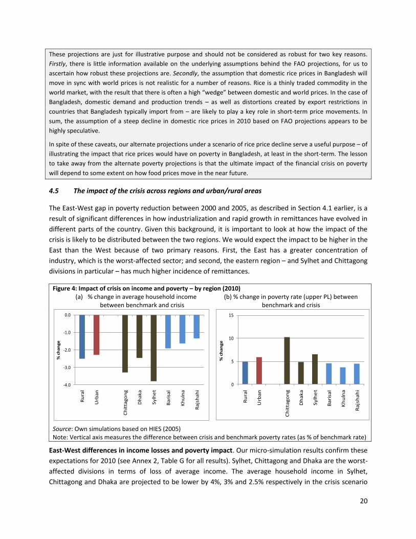
Figure 4: Impact of crisis on income and poverty – by region (2010) (a) % change in average household income

between benchmark and crisis (b) % change in poverty rate (upper PL) between

benchmark and crisis

Source: Own simulations based on HIES (2005) Note: Vertical axis measures the difference between crisis and benchmark poverty rates (as % of benchmark rate)

East-West differences in income losses and poverty impact. Our micro-simulation results confirm these

expectations for 2010 (see Annex 2, Table G for all results). Sylhet, Chittagong and Dhaka are the worst-

affected divisions in terms of loss of average income. The average household income in Sylhet,

Chittagong and Dhaka are projected to be lower by 4%, 3% and 2.5% respectively in the crisis scenario

-4.0

-3.0

-2.0

-1.0

0.0

Ru

ral

Urb

an

Ch

itta

go

ng

Dh

ak

a

Sy

lhe

t

Ba

risa

l

Kh

uln

a

Ra

jsh

ah

i

% c

ha

ng

e

0

5

10

15

Ru

ral

Urb

an

Ch

itta

go

ng

Dh

ak

a

Sy

lhe

t

Ba

risa

l

Kh

uln

a

Ra

jsh

ah

i

% c

ha

ng

e

21

compared to the benchmark in 2010, while the losses are less than 2% for Khulna, Rajshahi and Barisal

(Figure 4a). This is because the East is projected to suffer larger losses in remittances and labor incomes

compared to the West (see Annex 2, Table G). The fact that remittances are more common in the East

also implies that loss in remittances affects a larger share of the population than in the West.

Consistent with the projected income losses, the impact on poverty is higher in the East as well

compared to the West. The percentage increase in poverty rate due to the crisis (compared to the

benchmark) is projected to be the highest in Chittagong followed by Sylhet and Dhaka, and smaller for

the other divisions (Figure 4b). The percentage increase in extreme poverty rate (not shown here) is high

for Chittagong and Sylhet divisions, and much lower for the other divisions including Dhaka. Chittagong

and Sylhet are the highest recipients of international remittances by a large margin.26 As a result the

projected income loss in 2009 and 2010 due to the crisis (relative to the benchmark) is the highest in

Chittagong and Sylhet, which in turn leads to high poverty impact in these divisions.

Even after taking into account the significantly higher impact of the crisis in the East, the East-West gap

in poverty and income levels would continue to remain large in 2010. This is because the gaps in 2005 –

the baseline year for all the simulations – were large to start with (Figure 5). Khulna, Rajshahi and Barisal

are projected to remain as the poorer divisions of the country due to a slow rate of poverty reduction

during 2005-2010. The crisis is however expected to moderate the rapid poverty reduction that would

have otherwise occurred in Sylhet, Chittagong and Dhaka due to rapid industrial growth and rise in

remittances.

Figure 5: Poverty headcount rates for divisions (%) 2005 estimates & 2010 projections

Figure 6: Poverty headcount rates for urban/rural 2005 estimates & 2010 projections

Source: Estimates and simulations based on HIES (2005)

Rural-urban differences in impact. Our model does not project stark differences in the income and

poverty impact of the crisis between rural and urban areas. The loss in average household income due

to the crisis, as a percentage of benchmark income, is slightly higher in rural areas (2.5%) than urban

areas (2.3%). The main source of income loss is the drop in remittances, which is slightly higher (as a

percentage of benchmark remittances) in rural areas than in urban areas. The projected loss in labor

26

For example in 2005, 24% and 16% of households in Chittagong received remittances, compared to 9% of households nationally (World Bank 2008).

-

10

20

30

40

50

60

Ch

itta

go

ng

Dh

aka

Sylh

et

Ba

risa

l

Kh

uln

a

Ra

jsh

ah

i

Po

ve

rty

HC

R (

%)

-

10

20

30

40

50

Rural Urban

Po

ve

rty

HC

R (

%)

2005 2010 benchmark (no crisis) 2010-crisis

22

income, which accounts for a smaller share of income losses than remittances, is around 1.9% in urban

areas and 1.4% in rural areas (Annex 2, Table E).

The poverty headcount rate is expected to increase by 1.3 and 1.1 percentage points in rural and urban

areas, respectively, due to the crisis (Figure 6; full results in Annex 2, Table E). The extreme poverty rate

will be raised by 1.0 and 0.7 percentage points, respectively. However, as a percentage of the

benchmark poverty rates, the rate of increase in poverty and extreme poverty is higher in urban areas

than rural areas (Figure 4b). This happens because even though the amounts of change are similar for

urban and rural areas, the benchmark poverty rates are significantly lower in urban areas.

4.6 Distributional impact of the crisis – going beyond poverty and inequality indices

By generating predicted levels of income and consumption for all households in benchmark and crisis

scenarios, our simulation model allows us to examine the type of households that are likely to be

affected by the crisis, the primary channels of impact and their relative importance, and the distribution

of the impact across different income/consumption groups. Here we present the results from three

types of analysis that have been selected primarily for illustrative purposes, taking into account some of

the key issues relevant to Bangladesh. While the same analysis can be done for both years, for

illustrative purposes we choose to present the results for 2010 only, when the relatively larger impact of

the crisis is expected.

First, we examine the characteristics of the group we will call “crisis-vulnerable”, which refers to

households that would not have been poor in 2010 had there been no crisis. Second, we use the well-

known analytical device of growth incidence curves to see how change in consumption, as a result of the

crisis, is distributed across the distribution and between urban/rural areas and regions. Third, we

construct a few transition matrices to look at upward and downward movement of households as a

result of the crisis, compared to the benchmark. These are but examples of what is possible in the way

of distributional analysis with the results of our model; the choice of what type of analytics needs to be

done for a certain country would depend on the specific country context and policy concerns.

A profile of the “crisis-vulnerable”. Households that are expected to be in poverty in the crisis scenario

but not in the benchmark scenario in 2010 constitute around 1.2% of the population (1.8 million

individuals).27 These households, who are the “crisis-vulnerable”, are projected to suffer large income

losses due to the crisis, relative to the benchmark scenario – with a 23% drop in average household

income that translates to a 39% fall in average per capita consumption. The income loss is mainly due to

the loss of external remittances. While labor income loss amounts to around 2% of benchmark income,

the loss in non-labor income is around 67%, which is in turn due to a combination of declines in the

share of households receiving remittances and the average amount of remittances conditional on

27

Our simulation method, because of the way remittances are assigned with and without crisis, ensures that almost every household who is poor in the benchmark scenario will be poor in the crisis scenario as well, and conversely, almost every household that is non-poor in the crisis scenario will be non-poor in the benchmark scenario as well. For the sake of simplicity and realism alike, this appears to be a reasonable result.

23

receiving. The key characteristics of crisis-vulnerable households, relative to the rest of the population,

are as below (see Annex 2, Table F for all results).

Firstly, the crisis-vulnerable households have much higher incidence of external remittances than the

general population– 46% of the crisis-vulnerable households receive remittances from abroad in the

benchmark scenario compared to 10% of the general population. Secondly, the crisis-vulnerable have

larger household size and dependency than the rest of the population. Thirdly, they have lower skills on

the average – 89% of household heads have education of 0-9 years compared to the national average of

79%. Fourthly, a much higher share of adults in crisis-vulnerable households are employed in industry

and services (73% of total adults employed) compared to the general population (61% of total adults

employed). Finally, they look fairly similar to the general population in terms of their rural-urban

composition, with 80% from rural areas compared to 75% for the general population.

How do the crisis-vulnerable households compare with the permanently or structurally poor (defined as

the households who are poor in both benchmark and crisis scenarios in 2010)? Crisis-vulnerable

households have, on the average, lower dependency and higher skill level than the structurally poor.

Their employment rate in industry and services is also much higher – 73% of all employed adults in

crisis-vulnerable households are employed in these two sectors compared with 54% in the case of the

structurally poor. The crisis-vulnerable households are also significantly less rural than the structurally

poor households (see Annex 2, Table F).

In sum, the loss of (or reduction in) remittances from abroad is the most significant channel of impact

for households who are predicted to become poor as a direct result of the crisis. In fact, nearly 60% of

the aggregate poverty impact of the crisis in 2010 is due to the loss in remittances. It is important to

note that “loss of remittances” actually refers to the reduction in potential remittances in 2010 –

remittances, while still growing even during the crisis, will do so at a lower rate than what was expected

without the crisis (resulting in 10% lower remittances).

The profile of crisis-vulnerable households is consistent with our a priori intuition. Compared to the

general population, households vulnerable to the crisis are disproportionately employed in the non-

agricultural sectors because output and income losses are expected to occur in these sectors. They also

have “worse” attributes (larger households, higher dependency and lower skills) compared to the

general population – attributes that would make them vulnerable to being poor as a result of the crisis.

The crisis-vulnerable or the “newly poor” households as a result of the crisis are also different in a

number of key aspects from the more permanently poor. Compared to the structurally poor, they have

“better” characteristics (lower dependency, higher skills, receiving remittances, living in urban areas and

employed outside agriculture) – characteristics that our simulations indicate would have taken them out

of poverty had there been no crisis.

Growth incidence between benchmark and crisis scenarios. We use growth incidence curves (GICs) to

examine how the reductions in per capita consumption and income between benchmark and crisis

scenarios in 2010 are distributed. GICs are commonly used to look at the distribution of growth over

time; however the same concept is useful to see changes between two “states” of the world as well, in

24

this case the benchmark (no-crisis) and crisis states for the same point in time. A GIC in this case will plot

the percentage change in per capita consumption between 2010 benchmark and crisis scenarios for

every centile in the benchmark distribution of per capita consumption/income.28

Taking the country as a whole, the reduction in per capita expenditures due to the crisis (as a

percentage of benchmark expenditures) rises as one moves up the distribution, with the largest

difference (a drop of 4-5% in per capita consumption) occurring for households above the 70th percentile

of the benchmark distribution (Figure 7a). The drop in per capita consumption is less than 1% for

households in the bottom 10% of the distribution, but 3-4% for households in the 50th to 70th percentile.

There are interesting differences between how the impact of the crisis would be distributed within

urban and rural areas (Figure 7b). Three key differences stand out: (i) in rural areas, the largest impact is

seen among the richest (above the 80th percentile), while in urban areas those between the 50th and 80th

percentiles suffer the largest loss; (ii) the rural rich suffer a much steeper drop in consumption than the

urban rich; (iii) the moderately poor and near-poor in urban areas (10th to 40th percentiles) are affected

more than the corresponding group in the rural areas. These differences are mainly explained by high

dependence of the rural rich on external remittances, and the fact that the moderately poor and the

middle-class in urban areas depend more on income from the industry sector than do their rural

counterparts.29

Figure 7: Growth incidence curves (crisis vs. benchmark, 2010)

(a) Per capita expenditure: Bangladesh

(b) Per capita expenditure: urban and rural

Source: Own simulations based on HIES (2005) Note: 1) GICs have been smoothed to eliminate sharp kinks in the original curves 2) Percentiles on the X-axis are applicable to the relevant group (national, urban, rural, etc.)

Thus the impact of the crisis is higher for the better-off and particularly for the top 30% of the

distribution. The loss in welfare among the richest 10% of the rural population is larger than that for the

28

A “centile” refers to 1% of the population, when the households are ordered by per capita consumption/income. 29

It is important to note that the percentiles of expenditures are defined with reference to each area (urban or rural). Since urban areas are better off on the average than rural areas, the k-th percentile of urban households is better off than (and thus not strictly comparable with) the same percentile of rural households.

-6.0

0-5

.00

-4.0

0-3

.00

-2.0

0-1

.00

0.0

0

% C

ha

ng

e

0 10 20 30 40 50 60 70 80 90 100

Percentile

-6.0

0-5

.00

-4.0

0-3

.00

-2.0

0-1

.00

0.0

0

% C

ha

ng

e

0 10 20 30 40 50 60 70 80 90 100

Percentile

Urban Rural

25

equivalent group in urban areas, while the losses among the moderate and near poor in urban areas are

higher than that among the equivalent group in rural areas. The impact is lowest among the extreme

poor in both urban and rural areas, just because the extreme poor are the least likely to receive

remittances or work in industry even in the absence of the crisis.

GICs are also used to examine the incidence of change in per capita labor income in each sector (see

Annex 2, Figure A-1). As expected, there is no change in labor income for agricultural workers. Labor

income in industry falls across the board, which suggests that losses are distributed at a similar rate

(relative to their income in the no-crisis scenario) among all those who are employed in this sector. The

loss of income in the service sector is much lower and significant for only the bottom 10% of those who

earn any income from this sector.

Figure 8: Growth incidence curves (crisis vs. benchmark, 2010) by regions (East and West)

(a) Per capita expenditure by region

Source: Own simulations based on HIES (2005)

(b)Per capita labor income by region

Note: 1) GICs have been smoothed to eliminate sharp kinks in the original curves 2) The percentiles of consumption/income on the horizontal axis are for each region (East/West)

Finally, Figure 8(a) shows how the change in consumption due to the crisis is distributed within the two

regions (East and West). The results in Section 4.5 have shown that the adverse impact on incomes and

poverty is projected to be larger in the East than the West, with the most significant impacts expected in

Sylhet and Chittagong due to their high dependence on remittances. Figure 8(a) shows that the negative

impact of the crisis on consumption is larger in the East all along the distribution and worsens sharply as

one moves up the distribution, while the impact in the West is smaller and more evenly distributed. This

implies that the East-West gap with regard to impact of the crisis widens as consumption levels increase,

and is particularly significant for the 60th - 95th percentiles of the distributions.

Figure 8(b) shows that the East-West gap is not primarily due to differences in the household labor

income between the two regions, which are quite small. That said, richer individuals in the East (those in

the 60th-90th percentile) suffer larger labor income losses than their counterparts in the West, most

likely due to the concentration of industry in the East. The small gaps in labor income also suggest that

-6.0

0-5

.00

-4.0

0-3

.00

-2.0

0-1

.00

0.0

0

% C

ha

ng

e

0 10 20 30 40 50 60 70 80 90 100

Percentile

West: Barisal,Khulna & Rajshahi East: Chittagong, Dhaka & Sylhet

-6.0

0-5

.00

-4.0

0-3

.00

-2.0

0-1

.00

0.0

0

% C

ha

ng

e

0 10 20 30 40 50 60 70 80 90 100

Percentile

West: Barisal, Khulna & Rajshahi East: Chittagong, Dhaka & Sylhet

26

the East-West differences in Figure 8(a) are in a large part due to the impact of remittance decline,

which affects the East much more than the West.

Movements of households up or down the distribution due to the crisis. The GICs described above

provide a clear picture of the incidence of the losses in consumption due to the crisis across the entire

distribution. They also lead to some important follow-up questions from a distributional perspective:

where would the households suffering these losses end up relative to other households as a result of the

crisis, and what is the extent of “churning” that occurs in the distribution as a result of the crisis?

Transition matrices are useful to address such questions, by indicating movements up or down the

income/consumption distribution between the crisis and benchmark scenarios. These matrices are

constructed for deciles of per capita income and labor income, keeping the upper and lower limits of

each decile fixed at the benchmark income levels. This implies that movements up or down by

households in these matrices reflect the shifts that occur as a result of the crisis, relative to the

benchmark (no-crisis) income distribution (see Annex 2, Tables G.1 and G.2).

Figure 9 shows the share of households in each decile that (i) remain in the same decile, (ii) move up to

a higher decile or (iii) move down to a lower decile as a result of the crisis. Summing across all deciles,

93% of households are found to remain in the same decile by per capita income, while 96% do so for

deciles by per capita labor income. The deciles are derived from the benchmark distribution of

consumption or income, and kept unchanged for the crisis distribution. This implies that since the crisis

yields an overall loss of income, movements down are much more common than movements up.

The most significant downward movements occur for households in the upper middle range of the

distribution, namely in the 6th-9th deciles by per capita total income, with the largest movement

occurring for those in the 7th decile. The movements between deciles of per capita labor income are

smaller, with the largest movements occurring for the 7th and 8th deciles. Upward movements are

extremely rare.

Figure 9: Movements up and down the distribution due to crisis compared to the benchmark in 2010

Source: Own simulations based on HIES (2005)

Thus the negative impact of the crisis is high for the middle and upper middle class relative to that on

the poor and the richest. Between 8-12% of households in the 5th to 9th deciles of per capita income

move down to a lower decile as a result of the crisis. Labor income losses (that are significant enough to

0%

20%

40%

60%

80%

100%

1 2 3 4 5 6 7 8 9 10

Deciles

By deciles of per capita income

Stay in same decile Movement up Movement down

0%

20%

40%

60%

80%

100%

1 2 3 4 5 6 7 8 9 10

Deciles

By deciles of per capita labor income

Stay in same decile Movement up Movement down

27

lead to downward movements) are more narrowly concentrated among the upper middle class, likely

because the losses occur in the sectors (primarily industry) that produce relatively high incomes. The

fact that movements are less frequent when households are grouped by per capita labor income

suggests that a significant part of the movement in terms of total income is due to loss of remittances.

While there are some movements, more than 90% of all households remain in the same decile because

the aggregate income shock due to the crisis is quite low, due to the limited macroeconomic impact

projected for Bangladesh.

4.7 A limited validation of model using pre-crisis data for Bangladesh

How well does our model perform in estimating the impact of macroeconomic changes on poverty and

distribution? Addressing this question to our satisfaction will require a validation exercise that compares

our projections with actual post- (or during-) crisis estimates from a household survey, which must await

the availability of a survey conducted during or after the crisis. That said, a limited validation exercise

can be undertaken with available pre-crisis data.

In case of Bangladesh, such a validation involves using household data from an earlier year (HIES round

of 2000) to “project” poverty and other distributional estimates for 2005, and comparing these

projections to the actual estimates from HIES 2005. In practical terms this implies replicating the exact

same simulation method described in this paper on HIES 2000 data, using actual macroeconomic

statistics (growth rates of sectoral and aggregate GDP and remittance, and general and food CPI figures)

for the period 2000-2005, which are analogous to the macro projections used for the forward-looking

projections described above.

Table 5 shows the results of this simulation and

compares them with the actual estimates for

2005. The simulated poverty headcount rates are

within 1 percentage point of the actual estimates

for that year, with the difference between actual

and simulated rates being 0.7 and 0.3 percentage

points for moderate and extreme poverty rates,

respectively. The simulated results are also close

to the actual indices for depth (poverty gap) and

severity (squared gap) of moderate and extreme

poverty, as well as for the Gini index of inequality

in per capita expenditure.

The results suggest that the model does quite well

in simulating the distribution of expenditures and

poverty and inequality indices. Interestingly, all

the simulated indices, with the sole exception of

the (moderate) poverty headcount rate, are slightly above the actual values. This seems to indicate that

the simulation model underestimates the consumption growth for the poorest groups between 2000

Table 5: Poverty and inequality estimates for 2005 – simulated and actual

2000 2005

Simulated Actual

Moderate poverty

-Headcount rate 48.9 39.3 40.0

-Poverty gap 12.8 9.2 9.0

-Squared poverty gap 4.6 3.1 2.9

Extreme poverty -Headcount rate 34.3 25.4 25.1

-Poverty gap/depth 7.5 5.1 4.7

-Squared poverty gap 2.4 1.5 1.3

Inequality per-cap. Exp -Gini 0.31 0.33 0.31

-Theil 0.18 0.22 0.19

Source: HIES 2005; microsimulations using macro statistics and HIES 2000

28

and 2005. This is understandable, given that the poorest groups experienced unusually high

consumption growth during this period – per capita real consumption grew annually at 2.9% for the

bottom decile compared to 2.4% for the population.

Thus the validation based on historical data provides some confidence in the ability of the simulation

model to project future outcomes, linking macro statistics with econometric models built on household

data. However, important caveats apply to these results. Firstly, the validation has the benefit of using

actual macro data, whereas the 2009-2010 projections rely on macro projections. The ability of the

model to predict the future would then critically depend on the accuracy of the macro projections.

Secondly, the output-employment elasticities used for the validation are derived from the actual

employment data from HIES 2000 and 2005 and macro output statistics. The same elasticities are used

for our simulations for future years, but whether these will continue to be valid – particularly in a crisis

scenario that may lead to structural changes in the economy – is an important question that will matter

for the accuracy of our projections. Taken together, these caveats basically imply that with reliable

macroeconomic inputs and elasticities our model does well with household data for Bangladesh. While

this does not necessarily validate our future projections of poverty and distributional impact, a full

validation will only become possible when household data from 2009 or beyond becomes available.

5. Conclusion: implications of our results and extensions

Even with the caveats and limitations discussed in Section 3, our model appears to yield reasonable and

intuitively appealing results, based on a transparent and flexible approach using macro projections and

household survey data that are typically available in a developing country. The limited validation

exercise we conduct on pre-crisis data appears to suggest that the simulation results on poverty and

inequality from the model, based on real-world macroeconomic data for relevant years, are close to the

actual results. The impacts of the crisis on aggregate poverty and inequality estimates projected by the

model also appear to be consistent with those obtained using alternate, simpler approaches commonly

used by the Bank.

The value that our model adds to those simpler models is the ability to analyze potential distributional

impacts in detail, linking these changes to the channels through which the impact of the crisis is likely to

flow. The application of our model to Bangladesh also yields some useful insights relevant to the country

specifically, in two main areas discussed below: monitoring of impacts of the crisis and possible policies

to address these impacts.

Implications for Bangladesh in the context of the crisis. Firstly, our results suggest that in Bangladesh, a

select few indicators are prime candidates to monitor as real-time or “early-warning” indicators for the

poverty and distributional impact of the crisis. To be useful for rapid monitoring of poverty and

distributional impacts, the indicators must be easily obtained and measurable, sensitive to changes in

economic conditions, and correlated with changes in poverty and distribution. By these criteria, changes

in remittance flows from abroad, the movement of prices (including food prices) and movement of

wages by sector can serve as useful indicators for rapid monitoring. The extent of losses in foreign

remittances and labor income, and the price of food relative to other prices emerge from our

29

simulations as key determinants of the impact of the crisis on poverty.30 Loss of labor income in the

industry sector emerges as an important determinant of the impact as well. These indicators also have

the advantage of being relatively easy to monitor – with administrative or financial data (for

remittances), and quick market or household surveys (prices and wages).

The argument for tracking wages as a part of rapid monitoring, rather than other types of incomes or

employment, is twofold. First, growth slowdown in a country like Bangladesh is more likely to be

manifested in lower earnings rather than open unemployment – a hypothesis supported by our results

as well. Second, while wages represent only a part of the labor earnings from a sector, wages are much

easier to track (e.g. through quarterly labor force or even quick enterprise surveys) than income from

household enterprises and self-employment. Wages are also likely to be reasonably correlated with

broader measures of labor income, particularly in the industry sector where most of the labor market

impact is expected.

The same set of indicators is likely to be useful for tracking short-term poverty trends in Bangladesh

even if there were no crisis. Monitoring short-term changes in poverty and distribution, however,

becomes especially important during an economic shock or a crisis when rapid changes in welfare are

possible in a short timeframe that one would not expect in a “normal” year. The indicators suggested

here can be useful in predicting such changes when a crisis hits, as well as the size of these impacts and

how they are likely to be distributed in the population – given that real-time data on household income

or consumption to measure these impacts directly are usually unavailable.

Secondly, our results indicate that just focusing on poverty numbers would provide a partial view of the

distributional impact of the crisis in Bangladesh. The consumption/income impact is particularly

significant for the top half of the distribution and becomes progressively higher further up the

distribution. While public programs may not have much role to play to cushion the losses suffered by

the upper half of the distribution, these losses may have important political economy implications. The

prediction that the maximum impact in urban areas is likely to be on middle class households (50th to

80th percentiles of per capita consumption) may be particularly significant, since this group can have a

strong influence on public perceptions about economic hardship.

Thirdly, our results provide useful insights on the types of households who are likely to be poor as a

direct result of the crisis. Such households are found to have characteristics somewhat different from

those of the structurally poor, including a higher share of urban and non-agricultural sector workers.

This would imply that any intervention to mitigate the impact of the crisis on vulnerable households

would need to be modified (or designed differently) from that of the traditional safety net programs.

A discussion of what kinds of public policies and programs are best suited to mitigate the impact of the

crisis in Bangladesh is beyond the scope of this paper. A few broad statements can however be made

based on our results and what is known about existing safety net programs. Given that safety net

30

Around 70% of the aggregate poverty impact is driven by slowdown in growth of external remittances; the impact of the crisis in 2010 would be lower (by almost a third of the projected impact) if food prices were to decline relative to other prices (Box 1).

30

coverage is quite limited relative to the size of the poor population,31 there is little justification for using

the traditional programs to specifically target crisis-affected households, who appear to be better-

placed than the structurally poor households in terms of their endowments and access to economic

opportunities. As the impacts of the crisis take hold, there may be a case though for extending or

deepening certain types of existing programs (e.g. public works programs) in specific areas, regions or

sectors. Extending coverage among the urban poor, for instance, may address an important need, given

that the urban poor (10th to 40th percentiles) is likely to be one of the key affected groups and coverage

of existing safety net programs is extremely low in urban areas.

Implications for simulations in other countries. Clearly, our model is applicable to a number of country

contexts and for addressing a range of questions related to distributional impacts of an economic shock.

In terms of where this approach can be applied, the minimum data requirements include up-to-date

macroeconomic projections by sector, with and without crisis, and a fairly recent household survey with

income data that can be classified by sector. In addition to Bangladesh, this approach is currently being

attempted to assess crisis impacts in Philippines, Mexico and Egypt. While these countries share some of

the conditions with Bangladesh in terms of the potential channels of impact, the specific country and

data circumstances will also require the approach to be tailored somewhat to fit the relevant context.

Given the choice of models available to simulate the distributional impact of the crisis, it is also useful to

revisit the comparison between existing approaches and the model we have proposed here. The

comparison between our model and PovStat is the most relevant, given that both models have similar

data requirements. In our view, the choice of which model to use should be guided by the kind of

projections one needs to generate. In a situation where the impact on poverty and inequality measures

at the national and regional levels are all that is required and/or resources in terms of personnel and

time is limited, PovStat is likely to be the better and more practical choice. On the other hand, if more

detailed distributional impacts – including estimates on how the impact will be distributed across groups

or types of households and the sources of these impacts – are a concern, our model provides a feasible

approach. Even in that case, the robustness of the results can be tested by comparing the poverty and

inequality estimates generated from our model with those using PovStat, as it was done for Bangladesh.

Finally, decisions to extend or nuance the type of modeling approach used here would depend on the

availability of data and the specific country context. For example, the availability of more disaggregated

macroeconomic projections would allow for a more nuanced distributional analysis that is able to

capture movements within sectors and/or types of employment. The availability of better migration and

remittance data, particularly in the household survey, could allow for explicit modeling of remittances

and migration rather than the somewhat arbitrary assignment rule used here. Availability of surveys

conducted in 2009 (e.g. any labor force or rapid monitoring survey) that hint at some of the impacts of

the ongoing crisis would be useful in fine-tuning some of our analysis, particularly to take into account

any sudden price movements or structural changes in the labor market.

31

Around 13% of households, including around 5% of urban households, benefited from at least one safety net program in 2005; 8% of all households benefited from targeted programs (Chapter 6, World Bank 2008).

31

References

Alatas, V., and F. Bourguignon (2005). “The evolution of Income distribution during Indonesia’s fast

growth, 1980-96” in The microeconomics of income distribution dynamics in East Asia and Latin

America, eds. Bourguignon, F., Ferreira, F., and Lustig, N., Washington DC: Oxford University Press

and The World Bank.

Beach, Ch. (1989). “Dollars and Dreams: A reduced middle class? Alternative Explanations”, Journal of

Human Resources, 24, 162-193

Blackburn, M. and D. Bloom (1987). “Earnings and income inequality in the United States”, Population

Development Review, pp. 575-609

Bourguignon, F. and F. Ferreira (2005). “Decomposing Changes in the Distribution of Household

Incomes: Methodological Aspects” in The microeconomics of income distribution dynamics in East

Asia and Latin America, eds. Bourguignon, F., Ferreira, F., and Lustig, N., Washington DC: Oxford

University Press and The World Bank.

Bourguignon, F. and F. Ferreira (2003). “Ex-ante evaluation of policy reforms using behavioral models” in

The Impact of Economic Policies on Poverty and Income Distribution, Bourguignon, F. and Pereira da

Silva, L. (eds), World Bank-Oxford University Press.

Bourguignon, F., M. Bussolo and L. Pereira da Silva (2008). “Introduction: Evaluating the impact of

Macroeconomic Policies on Poverty and Income Distribution”, in The Impact of Macroeconomic

Policies on poverty and Income Distribution, eds. Bourguinon, F., Bussolo, M. and Pereira da Silva, L.

Washington DC, The World Bank.

Burkhauser, R., A. Crews, A. Daly and S. Jenkins (1999). “Testing the significance of income distribution

changes over the 1980s business cycle: a cross-national comparison”, Journal of Applied

Econometrics, 14, pp 253-272

Chen, S. and M. Ravallion (2009). “The Impact of the Global Financial Crisis on the World’s Poorest”.

World Bank Development Research Group.

Deaton, A. (2001). Intervention in a panel discussion on the International Monetary Fund – sponsored

conference on “Macroeconomic Policies and Poverty Reduction” April, 13, 2001, Washington D.C;

transcript at http://www.imf.org/external/np/tr/2001/tr0104143.htm

Ferreira, F., P. Leite, L. Pereira da Silva and P. Picchetti (2008). “Can the Distributional Impacts of

Macroeconomic Shocks Be Predicted? A Comparison on Top-Down Macro-Micro Models with

Historical Data for Brazil” in The Impact of Macroeconomic Policies on poverty and Income

Distribution, eds. Bourguinon, F., Bussolo, M. and Pereira da Silva, L. Washington DC, The World

Bank.

Jenkins, S. (1995). “Did the middle class shrink during the 1980s? UK evidence from kernel density

estimates”, Economics letters, 49, 407-413

Levy, F. and R. Murnane (1992). “U.S. Earnings levels and earnings inequality: A review of recent trends

and proposed explanations”, Journal of Economic Literature, Vol XXX

32

Paci, P. and M. Sasin (2009). “Making Work Pay in Bangladesh: Employment, Growth, and Poverty

Reduction”. World Bank Directions in Development: Poverty.

Paci, P., B. Rijkers, and A. Seinaert (2008). "Crunch Time in the Developing World Too? Policy options for

dealing with the potential poverty and distributional impact of the financial crisis". World Bank

Poverty Reduction Group, PRMVP.

Ravallion, M. (2009). "The Developing World's Bulging (But Vulnerable) Middle Class". Policy Research

Working Paper 4816. World Bank. Washington DC

Vos, R., L. Taylor, L and R. Paes de Barro eds. (2002) Economic liberalization, distribution and poverty.

Latin America in the 1990’s. UNDP

World Bank (2007). Bangladesh: Strategy for Sustained Growth. Bangladesh Development Series. Paper

No. 18. Dhaka.

World Bank (2008). Poverty Assessment for Bangladesh: Creating Opportunities and Bridging the East-

West Divide. Report No. 44321-BD. Washington DC.

World Bank (2009). Welfare Impact of Rising Food Prices in South Asian Countries. Policy Note, South

Asia Economic Policy and Poverty Unit. Washington DC

World Bank PovertyNet website. “PovStat” (Accessed August 12, 2009).

http://web.worldbank.org/WBSITE/EXTERNAL/TOPICS/EXTPOVERTY/EXTPSIA/0,,contentMDK:20483029

~isCURL:Y~menuPK:1108016~pagePK:148956~piPK:216618~theSitePK:490130,00.html

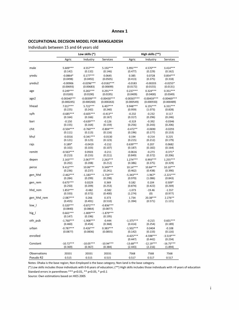
i

Annex 1

OCCUPATIONAL DECISION MODEL FOR BANGLADESH

Individuals between 15 and 64 years old

Notes: Dhaka is the base region; Non-Employed is the base category; Non-land is the base category.

(*) Low skills includes those individuals with 0-8 years of education; (**) High skills includes those individuals with >9 years of education

Standard errors in parentheses *** p<0.01, ** p<0.05, * p<0.1

Source: Own estimations based on HIES 2005

Low skills (*) High skills (**)

Agric Industry Services Agric Industry Services

male 5.609*** 4.557*** 5.192*** 5.991*** 4.570*** 3.414***(0.142) (0.132) (0.146) (0.477) (0.229) (0.162)

yredu -0.0864* 0.177*** 0.0645 0.385 0.0728 0.854***(0.0498) (0.0492) (0.0505) (0.413) (0.375) (0.318)

yredu2 -0.00906 -0.0296*** -0.0182*** -0.0183 -0.00203 -0.0255*(0.00693) (0.00683) (0.00699) (0.0172) (0.0155) (0.0131)

age 0.249*** 0.265*** 0.291*** 0.237*** 0.324*** 0.351***(0.0183) (0.0190) (0.0195) (0.0409) (0.0400) (0.0349)

age2 -0.00340*** -0.00399*** -0.00430*** -0.00307*** -0.00459*** -0.00469***(0.000245) (0.000260) (0.000263) (0.000549) (0.000550) (0.000489)

hhead 7.017*** 5.722*** 6.407*** 9.948*** 6.191*** 6.331***(0.225) (0.242) (0.240) (0.959) (1.073) (0.828)

sylh -0.685*** -0.605*** -0.413** -0.232 -0.232 0.117(0.164) (0.166) (0.167) (0.317) (0.296) (0.246)

bari -0.150 -0.639*** -0.126 -0.319 -0.392 -0.0346(0.155) (0.164) (0.159) (0.256) (0.243) (0.206)

chit -0.504*** -0.760*** -0.804*** -0.472** -0.0690 -0.0293(0.111) (0.113) (0.116) (0.196) (0.177) (0.153)

khul -0.0316 -0.341*** -0.0130 0.194 -0.214 0.225(0.121) (0.123) (0.123) (0.215) (0.212) (0.179)

rajs 0.189* -0.0419 -0.152 0.639*** 0.207 0.0682(0.102) (0.103) (0.107) (0.187) (0.182) (0.164)

remitt -0.563*** 0.0503 -0.211 -0.0616 -0.273 -0.371*(0.213) (0.155) (0.211) (0.849) (0.372) (0.206)

depen 2.163*** 2.067*** 2.263*** 1.274*** 0.993*** 1.255***(0.202) (0.208) (0.212) (0.386) (0.375) (0.329)

perce 9.412*** 10.06*** 9.349*** 10.14*** 10.84*** 10.10***(0.236) (0.237) (0.241) (0.462) (0.438) (0.390)

gen_hhd -2.462*** -1.183*** -1.733*** -5.343*** -1.967* -2.221***(0.284) (0.299) (0.298) (0.970) (1.086) (0.843)

gen_rem 0.675*** 0.0229 0.369 0.182 0.104 0.509*(0.250) (0.209) (0.253) (0.874) (0.422) (0.269)

hhd_rem 1.853*** -0.482 -0.582 -1.073 -19.46 -1.557(0.333) (0.372) (0.400) (1.274) (0) (0.977)

gen_hhd_rem -2.087*** 0.266 0.373 1.734 20.38*** 2.276**(0.455) (0.491) (0.510) (1.394) (0.571) (1.121)

low_l 0.320*** -0.872*** -0.836***(0.0840) (0.0864) (0.0877)

hig_l 0.665*** -1.809*** -1.879***(0.147) (0.196) (0.195)

oth_pub -1.760*** -1.908*** -0.444 -1.375*** -0.215 0.601***(0.460) (0.454) (0.368) (0.414) (0.254) (0.189)

urban -0.787*** 0.426*** 0.383*** -1.502*** 0.0404 -0.108(0.0877) (0.0836) (0.0855) (0.142) (0.133) (0.116)

enrolled -4.425*** -4.598*** -3.519***(0.447) (0.442) (0.234)

Constant -10.72*** -10.05*** -10.94*** -13.68*** -12.19*** -16.75***(0.369) (0.367) (0.384) (2.443) (2.216) (1.894)

Observations 20331 20331 20331 7568 7568 7568

Pseudo R2 0.515 0.515 0.515 0.517 0.517 0.517

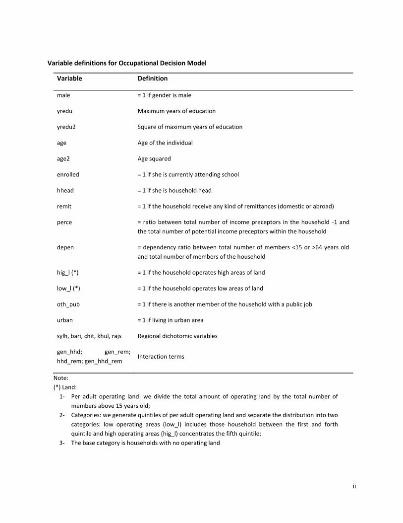
ii

Variable definitions for Occupational Decision Model

Variable Definition

male = 1 if gender is male

yredu Maximum years of education

yredu2 Square of maximum years of education

age Age of the individual

age2 Age squared

enrolled = 1 if she is currently attending school

hhead = 1 if she is household head

remit = 1 if the household receive any kind of remittances (domestic or abroad)

perce = ratio between total number of income preceptors in the household -1 and

the total number of potential income preceptors within the household

depen = dependency ratio between total number of members <15 or >64 years old

and total number of members of the household

hig_l (*) = 1 if the household operates high areas of land

low_l (*) = 1 if the household operates low areas of land

oth_pub = 1 if there is another member of the household with a public job

urban = 1 if living in urban area

sylh, bari, chit, khul, rajs Regional dichotomic variables

gen_hhd; gen_rem;

hhd_rem; gen_hhd_rem Interaction terms

Note:

(*) Land:

1- Per adult operating land: we divide the total amount of operating land by the total number of

members above 15 years old;

2- Categories: we generate quintiles of per adult operating land and separate the distribution into two

categories: low operating areas (low_l) includes those household between the first and forth

quintile and high operating areas (hig_l) concentrates the fifth quintile;

3- The base category is households with no operating land

iii

LOG EARNING EQUATIONS (Individuals between 15 and 64 years old)

Notes: Dhaka is the base region;

Non-land is the base category

(*) Low skills includes those individuals with 0-8 years of education

(**) High skills includes those individuals with more than 9 years of education

Standard errors in parentheses *** p<0.01, ** p<0.05, * p<0.1

Source: Own estimations based on HIES 2005

Low skills (*) High skills (**)

Agric Industry Services Agric Industry Services

male 1.271*** 0.915*** 0.785*** 1.072*** 0.751*** 0.245***(0.0405) (0.0407) (0.0481) (0.214) (0.128) (0.0517)

yredu 0.0228*** 0.0396*** 0.0357*** 0.128*** 0.119*** 0.0934***(0.00481) (0.00474) (0.00464) (0.0256) (0.0148) (0.00737)

age 0.0549*** 0.0555*** 0.0730*** 0.0678*** 0.0996*** 0.0625***(0.00559) (0.00702) (0.00739) (0.0221) (0.0187) (0.0103)

age2 -0.000666*** -0.000683*** -0.000867*** -0.000831*** -0.00114*** -0.000582***(7.12e-05) (9.20e-05) (9.47e-05) (0.000273) (0.000240) (0.000130)

sylh 0.0877 0.0466 0.0690 0.205 0.414*** 0.208***(0.0608) (0.0617) (0.0569) (0.229) (0.146) (0.0705)

bari 0.0335 -0.222*** 0.0960* 0.211 0.0728 -0.0678(0.0528) (0.0638) (0.0522) (0.177) (0.115) (0.0603)

chit 0.175*** 0.176*** 0.298*** 0.291** 0.261*** 0.267***(0.0391) (0.0410) (0.0418) (0.143) (0.0837) (0.0472)

khul 0.119*** -0.332*** -0.102** 0.264* -0.269*** -0.174***(0.0425) (0.0458) (0.0411) (0.138) (0.103) (0.0519)

rajs 0.127*** -0.375*** -0.239*** 0.103 -0.254*** -0.191***(0.0345) (0.0356) (0.0376) (0.114) (0.0801) (0.0493)

sala 0.228*** -0.158*** -0.190*** 0.656*** -0.179*** -0.222***(0.0303) (0.0314) (0.0287) (0.138) (0.0613) (0.0401)

low_l 0.200*** 0.729***(0.0310) (0.121)

hig_l 0.750*** 1.506***(0.0454) (0.135)

urban 0.00610 0.0702** 0.0653** 0.378*** 0.133** 0.163***(0.0364) (0.0278) (0.0272) (0.104) (0.0628) (0.0352)

hhead 0.180*** 0.0656 0.0806 0.0452(0.0406) (0.0418) (0.0812) (0.0468)

ind_exp 0.0627* 0.0698(0.0331) (0.0696)

public 0.404*** 0.254***(0.0724) (0.0426)

Constant 4.594*** 5.847*** 5.593*** 2.889*** 4.284*** 5.597***(0.115) (0.132) (0.138) (0.495) (0.353) (0.195)

Observations 4734 2384 2700 802 759 1938

R-squared 0.272 0.376 0.262 0.247 0.319 0.281

Adj R-squared 0.270 0.372 0.259 0.235 0.307 0.277

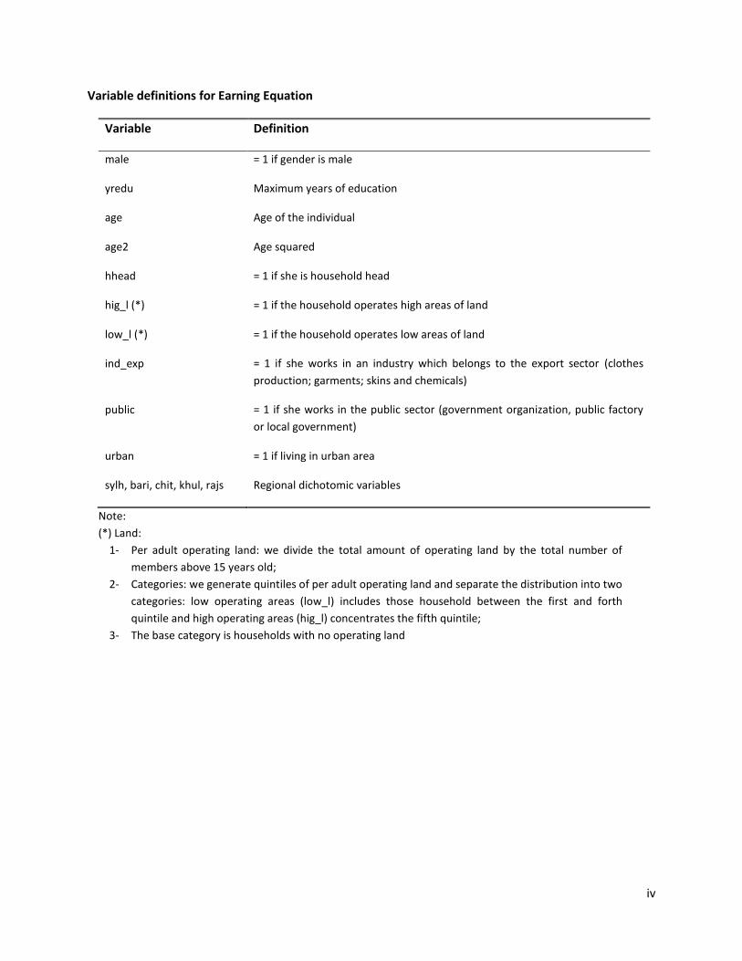
iv

Variable definitions for Earning Equation

Variable Definition

male = 1 if gender is male

yredu Maximum years of education

age Age of the individual

age2 Age squared

hhead = 1 if she is household head

hig_l (*) = 1 if the household operates high areas of land

low_l (*) = 1 if the household operates low areas of land

ind_exp = 1 if she works in an industry which belongs to the export sector (clothes

production; garments; skins and chemicals)

public = 1 if she works in the public sector (government organization, public factory

or local government)

urban = 1 if living in urban area

sylh, bari, chit, khul, rajs Regional dichotomic variables

Note:

(*) Land:

1- Per adult operating land: we divide the total amount of operating land by the total number of

members above 15 years old;

2- Categories: we generate quintiles of per adult operating land and separate the distribution into two

categories: low operating areas (low_l) includes those household between the first and forth

quintile and high operating areas (hig_l) concentrates the fifth quintile;

3- The base category is households with no operating land

v

Annex 2

Table A.1: POPULATION GROWTH CHANGE

(in millions - medium variant)

Table A.2: SECTORAL OUTPUT GROWTH CHANGE

(Base: 1995-96 = 100; Taka in Millions)

Table A.3: EMPLOYMENT SECTORAL GROWTH CHANGE

0-14 15-64 +65 Total

Total 51.81 95.76 5.55 153.12

Male 26.36 48.36 2.76 77.48

Female 25.45 47.40 2.79 75.64

Total 50.76 107.15 6.51 164.42

Male 25.83 54.18 3.13 83.13

Female 24.93 52.98 3.39 81.29

Total (2.03) 11.89 17.39 7.38

Male (2.02) 12.02 13.46 7.29

Female (2.04) 11.76 21.37 7.47

Source:World Population Prospects - The 2008 revision - UN Population Division

2005

2010

%

2009 2010 2009 2010 09 vs 05 10 vs 05 09 vs 05 10 vs 05

2,560,897 3,311,735 3,546,604 3,286,805 3,469,363 29.3 38.5 28.3 35.5

Agriculture 570,367 674,336 700,754 678,417 702,840 18.2 22.9 18.9 23.2

Industry 724,890 985,917 1,077,113 976,016 1,034,577 36.0 48.6 34.6 42.7

Services 1,265,640 1,651,482 1,768,737 1,632,371 1,731,946 30.5 39.8 29.0 36.8

Total 5.93 6.62 7.09 5.82 5.55 (0.8) (1.5)

Agriculture 2.21 4.00 3.92 4.63 3.60 0.6 (0.3)

Industry 8.28 7.00 9.25 5.93 6.00 (1.1) (3.2)

Services 6.36 7.50 7.10 6.25 6.10 (1.2) (1.0)

Remittances (US$ mill ions) 3,848 9,689 10,872 10,000 12,100 151.8 182.5 159.9 214.4

Source: BBS - GDP of Blangadesh 2008 and Projections

TOTAL

Benchmark2005

GDP in

constant

prices

Annual

Growth rate

Crisis % Crisis% Benchmark

HIES 2005

Individuals 15-64 years old

Millions % Millions % Millions % Millions % Millions %

Total 79.7 89.6 89.6 89.6 89.6

Non-employed 41.1 51.6 45.1 50.3 43.3 48.4 45.3 50.6 43.9 49.0

Employed 38.5 48.4 44.5 49.7 46.2 51.6 44.3 49.4 45.7 51.0

Agriculture 17.1 44.3 17.9 40.1 18.0 39.0 17.9 40.4 18.0 39.5

Industry 9.2 23.8 10.6 23.8 11.0 23.9 10.5 23.8 10.3 22.5

Services 12.3 32.0 16.1 36.1 17.2 37.2 15.9 35.8 17.4 38.0

Source: BBS - GDP of Blangadesh 2008 and Projections

2005 Benchmark2009

Crisis2010 20102009

vi

Table B- DEMOGRAPHIC, HOUSEHOLD INCOME & LABOR MARKET OVERVIEW

Table C- FOOD PRICES COMPARED TO OVERALL CPI

Quantity % Quantity % Quantity % Quantity % Quantity %

Population (million)

- Total 138.8 149.1 149.1 149.1 149.1

- Urban 34.3 24.7 36.9 24.8 36.9 24.8 36.9 24.8 36.9 24.8

- Working-age (1)81.9 59.0 92.0 61.7 92.0 61.7 92.0 61.7 92.0 61.7

Household Income (Tk/month)

- Total 7,229.5 100.0 8,290.6 100.0 8,751.2 100.0 8,229.0 100.0 8,539.1 100.0

- Labor income (2)4,933.2 68.2 5,522.8 66.6 5,792.8 66.2 5,493.9 66.8 5,701.7 66.8

- Non-labor income (3)1,757.5 24.3 2,226.2 26.9 2,416.8 27.6 2,193.5 26.7 2,295.9 26.9

Remittances 676.7 9.4 1,102.5 13.3 1,262.8 14.4 1,073.0 13.0 1,151.8 13.5

- Implicit rent 538.9 7.5 541.5 6.5 541.5 6.2 541.5 6.6 541.5 6.3

Working-age (million) (1)

- Labor Force 79.7 100.0 89.6 100.0 89.6 100.0 89.6 100.0 89.6 100.0

Non-employed 41.1 51.6 45.1 50.3 43.3 48.4 45.3 50.6 43.9 49.0

Employed 38.5 48.4 44.5 49.7 46.2 51.6 44.3 49.4 45.7 51.0

- Mean earnings per worker

(Tk/month) (2)3,523.4 3,979.7 4,174.9 3,958.2 4,108.0

- Education status 79.6 100.0 89.5 100.0 89.5 100.0 89.5 100.0 89.5 100.0

Low skilled (4)59.5 74.8 67.4 75.3 67.4 75.3 67.4 75.3 67.4 75.3

High skilled (5)20.1 25.2 22.1 24.7 22.1 24.7 22.1 24.7 22.1 24.7

- Employment 38.5 100.0 44.5 100.0 46.2 100.0 44.3 100.0 45.7 100.0

Salaried (6)21.1 54.8 24.2 54.5 25.4 54.9 24.1 54.4 25.0 54.7

Self-employment 17.4 45.2 20.3 45.5 20.8 45.1 20.2 45.6 20.7 45.3

- Economic sectors 38.5 100.0 44.5 100.0 46.2 100.0 44.3 100.0 45.7 100.0

Agriculture 17.1 44.3 17.9 40.1 18.0 39.0 17.9 40.4 18.0 39.5

Industry 9.2 23.8 10.6 23.8 11.0 23.9 10.5 23.8 10.3 22.5

Services 12.3 32.0 16.1 36.1 17.2 37.2 15.9 35.8 17.4 38.0

Notes: (1) Individuals in 15-64 age category (2) Labor earnings from all activities

(3) Includes capital(rent land, property, profits, etc), remittances, social(insurances, charity, etc) and other non-labor income (4) Low-skilled = 0-9 years of education

(5) High-skilled = +10 years of education (6) Include daily wage and salaried workers

Source: Own estimations based on HIES 2005 and projections

Benchmark

201020092005

Crisis

2009 2010

General

(1)

Food

(2)

Non-Food

(3)

2005 100.0 100.0 100.0 1.81

Projection

2009 135.7 140.7 126.7 5.58

2010 144.8 152.0 131.9 6.86

2010 (*) 134.3 132.5 137.4 0.49

Variation

2009/05 35.7 40.7 41.7

2010/05 44.8 52.0 31.9

2010/05(*) 34.3 32.5 37.4

CPI - RuralFood vs Gral

Weight of food in CPI and Poverty Line (PL) in rural areas

CPI Food 62.96

Non-food 37.04

PL Rural Dhaka Food 67.10

Non-food 32.90

- % variation in PL '09 0.3093

- % variation in PL '10 0.4150

- % variation in PL '10 * (0.1086)

(*) Considers the international rice price forecast of FAO for 2010

Source: BBS - Consumer Price Index (CPI) and Inflation Rate several reports

vii

Table D.1: MAIN DISTRIBUTIVE RESULTS OF MACRO-MICRO SIMULATIONS

Table D.2: MAIN POVERTY & INEQUALITY RESULTS - DIFFERENT METHODOLGIES

2009 2010 2009 2010 2010*

Moderate poverty

-Headcount rate 40.0 28.2 24.6 28.6 25.8 25.4

-Poverty gap 9.0 5.9 5.0 6.0 5.3 5.2

-Severity of poverty 2.9 1.8 1.5 1.9 1.6 1.6

Extreme poverty

-Headcount rate 25.1 16.5 13.9 16.7 14.8 14.5

-Poverty gap 4.7 2.9 2.4 3.0 2.5 2.5

-Severity of poverty 1.3 0.8 0.6 0.8 0.7 0.7

Inequality per-cap. Exp

-Gini 0.310 0.321 0.324 0.341 0.320 0.320

-Theil 0.186 0.197 0.199 0.222 0.194 0.194

Notes: Benchmark = economy growth on trend

Crisis = financial crisis scenario

(*) Crisis with FAO rice prices forecast

(1) Per capita Expenditure

(2) Total labor income

(3) Main labor income

Source: Own estimations

2005Benchmark Crisis

2009 2010 2009 2010

Headcount Ratio

Povstat 40.0 28.7 25.1 28.9 26.3

Elasticity (1)40.0 27.4 24.4 28.0 25.6

Macro-micro simulation 40.0 28.2 24.6 28.6 25.8

Poverty Gap

Povstat 9.0 5.8 4.8 5.8 5.1

Macro-micro simulation 9.0 5.9 5.0 6.0 5.3

Severity of poverty

Povstat 2.9 1.7 1.4 1.7 1.5

Macro-micro simulation 2.9 1.8 1.5 1.9 1.6

Inequality per-cap. Exp (2)

Gini

Povstat 0.01 0.31 0.31 0.31 0.31

Macro-micro simulation 0.33 0.32 0.32 0.34 0.32

Theil

Povstat 0.19 0.19 0.19 0.18 0.18

Macro-micro simulation 0.21 0.20 0.20 0.22 0.19

Notes: (1) No food prices adjustment

(2) Non-comparable because Povstat calculates over household head distribution

Source: Own estimations & World Bank (2009)

Crisis2005

Benchmark

viii

TABLE E- POVERTY IMPACT BY AREA & REGION Table E.1: Household income (mean Tk/month at constant 2005 prices)

Table E.2: Poverty rate (% of population under Upper PL)

Table E.3: Extreme poverty rate (% of population under Lower PL)

Rural Urban Barisal Chittagong Dhaka Khulna Rajshahi Sylhet

Benchmark

Total income 8,751 7,506 12,421 7,602 11,114 9,720 6,906 6,439 11,600

Labor income 5,793 4,764 8,826 5,188 6,958 6,316 4,695 4,852 6,450

Remittances 1,263 1,326 1,078 881 2,514 1,318 563 296 3,461

Crisis

Total income 8,539 7,318 12,137 7,456 10,748 9,480 6,793 6,353 11,159

Labor income 5,702 4,699 8,657 5,115 6,836 6,208 4,633 4,788 6,347

Remittances 1,152 1,209 984 819 2,280 1,200 520 280 3,135

Loss of income with crisis (% of benchmark) -2.4 -2.5 -2.3 -1.9 -3.3 -2.5 -1.6 -1.3 -3.8

Loss of labor income (% of benchmark) -1.6 -1.4 -1.9 -1.4 -1.8 -1.7 -1.3 -1.3 -1.6

Loss of remittance (% of benchmark) -8.8 -8.8 -8.7 -7.1 -9.3 -8.9 -7.6 -5.5 -9.4

TOTALAREA REGION

20

10

20

10

Rural Urban Barisal Chittagong Dhaka Khulna Rajshahi Sylhet

HEADCOUNT

2005 40.0 43.8 28.4 52.0 34.0 32.0 45.7 51.2 33.8

Benchmark [B] 2010 24.6 26.7 18.1 37.8 12.4 19.2 31.7 36.5 16.3

Cris is [C] 2010 25.8 28.0 19.2 39.5 13.7 20.1 32.8 38.1 17.4

[C] - [B] as % of [B] 2010 5.1 4.9 5.9 4.6 10.2 4.8 3.7 4.5 6.5

TOTALAREA REGION

Rural Urban Barisal Chittagong Dhaka Khulna Rajshahi Sylhet

HEADCOUNT

2005 25.1 28.6 14.6 35.6 16.1 19.9 31.6 34.5 20.8

Benchmark [B] 2010 13.9 15.9 7.7 24.7 3.4 11.2 19.5 21.5 8.3

Cris is [C] 2010 14.8 16.9 8.4 25.8 4.3 11.9 20.7 22.6 9.3

[C] - [B] as % of [B] 2010 6.6 6.4 8.4 4.7 26.5 5.6 5.9 5.1 13.0

TOTALAREA REGION

ix

TABLE F- PEOPLE WHO ARE POOR "DUE" TO CRISIS - 2010

TABLE G- INCOME STATUS "CHANGES"

Household characteristics

Crisis-

Vulnerable

General

population

Structurally

poor

- Rural (%) 79.5 74.7 82.1

- No. of members 4.90 4.86 5.19

- Dependency ratio 0.42 0.39 0.48

- Employed (individuals)* 54.8 50.3 53.3

- Sectoral share of employment (% of total employed)

Agriculture 26.7 39.0 45.6

Industry 27.1 23.9 19.4

Services 46.2 37.2 35.0

Household head

- Age (mean) 40.98 45.57 43.47

- Male (%) 95.0 89.7 91.3

- Education level 0-9 years 87.9 79.1 94.3

Household income (Crisis-Vulnerable) Benchmark Crisis

- Income (mean)

Total Income (tk. 2005 prices) 6,741.2 5,165.2 23.4

Labor income 4,113.8 4,046.0 1.6

Non-labor income 2,268.0 759.9 66.5

- Remittances from abroad

% of household receiving 45.7 9.9 78.5

Mean conditional on receiving 1,681.1 178.9 89.4

Implicit rent 359.4 359.4 -

- Percapita Expenditure (mean) 1,278.9 785.9 38.5

Table G.1: Transition matrix: Benchmark - Crisis

Per-capita income

1 2 3 4 5 6 7 8 9 10

1 100.0

2 2.79 97.21

3 0.68 4.21 95.11

4 0.34 0.46 6.18 93.03

5 0.69 0.68 1.33 5.79 91.50

6 0.60 0.35 0.39 0.58 6.89 91.18

7 0.33 0.14 0.71 0.38 2.62 7.26 88.55

8 0.25 0.49 0.27 0.92 0.93 1.10 7.34 88.58 0.12

9 0.11 0.23 0.32 0.49 0.32 1.32 6.30 90.91

10 0.11 0.04 0.17 0.61 4.72 94.35

Table G.2: Transition matrix: Benchmark - Crisis

Per-capita Labor income

1 2 3 4 5 6 7 8 9 10

1 100.0

2 1.59 98.4

3 2.78 97.2

4 5.03 94.85 0.12

5 5.30 94.7

6 6.87 93.1

7 6.95 92.9 0.12

8 7.72 92.28

9 0.07 4.11 95.8

10 2.82 97.2

Ben

chm

ark

Crisis

Crisis

Ben

chm

ark

x

Figure A-1: GICs (crisis vs. benchmark, 2010) Per capita labor income by sector

Source: Own simulations based on HIES (2005) Note: 1) GICs have been smoothed 2) Percentiles of income (x-axis) refer to the relevant sector

-6.0

0-5

.00

-4.0

0-3

.00

-2.0

0-1

.00

0.0

0

% C

ha

ng

e

0 10 20 30 40 50 60 70 80 90 100

Percentile

Agriculture Industry Services