Embed Size (px)
Citation preview
_____________________________________________________________________
CREDIT Research Paper
No. 18/01
_____________________________________________________________________
Assessing Cohort Aggregation to Minimise Bias in
Pseudo-Panels
by
Rumman Khan
Abstract
Pseudo-panels allow estimation of panel models when only repeated cross-sections are
available. This involves grouping individuals into cohorts and using the cohort means
as if they are observations in a genuine panel. Their practical use is constrained by a
lack of consensus on how the pseudo-panels should be formed, particularly to address
potential sampling error bias. We show that grouping can also create substantial
aggregation bias, calling into question how well pseudo-panels can mimic panel
estimates. We create two metrics for assessing the grouping process, one for each
potential source of bias. If both metrics are above certain recommended values, the
biases from aggregation and sampling error are minimised, meaning results can be
interpreted as if they were from genuine panels.
JEL Classification: C13 C23 C81 D10 O12
Keywords: Pseudo-panel; Estimation bias; Sampling error; Aggregation bias;
Repeated Cross-Section; Household Surveys
_____________________________________________________________________
Centre for Research in Economic Development and International Trade,
University of Nottingham
_____________________________________________________________________
CREDIT Research Paper
No. 18/01
Assessing Cohort Aggregation to Minimise Bias in
Pseudo-Panels
by
Rumman Khan
Outline
1. Introduction
2. Sampling Error
3. Aggregation Bias
4. Implementing AWAR and CAWAR
5. Conclusion
References
Appendices (A, B & C)
The Authors
Rumman Khan is a Research Fellow at the School of Economics, University of
Nottingham. Contact: [email protected]
Acknowledgements
The author is grateful to Professors Oliver Morrissey and Sourafel Girma for their
comments, suggestions, and feedback. This work is based on PhD research supported
by the Economic and Social Research Council (ESRC), being developed as part of the
ESRC-DFID GCRF Project Pseudo-Panels for Long Period Analysis of African
Household Surveys (ES/P003389/1).
_____________________________________________________________________
Research Papers at www.nottingham.ac.uk/economics/credit/
Assessing Cohort Aggregation
1
1. Introduction
The advantages of using panel datasets, which include both time-series and cross-
section dimensions, for empirical analysis are well known. However, in many settings
such data may not be available due to the cost and difficulty of following the same set
of individual agents over a sufficiently long period of time. Instead, what often is
available is repeated cross-sections (henceforth RCS) where a different set of
individuals are observed in each time period. Many household surveys, particularly
those covering a long time span, are of this form. This is especially true in developing
countries where, since the 1980s, many such surveys have been conducted under the
World Bank’s Living Standards Measurement Survey (LSMS) project. Consequently,
pseudo-panels have increasing been used as they allow for panel-type estimation with
RCS data.
By grouping individuals into cohorts based on common characteristics that are fixed
over time, pseudo-panels can be created by treating the cohort means as if they are
observations in an actual panel. This method was first developed by Deaton (1985) in
order to estimate a linear fixed effects model. The literature has since expanded to
incorporate more complex models that otherwise could only be estimated using panel
data. Examples include dynamic models (Moffitt, 1993; Girma, 2000; Verbeek and
Vella 2005), duration analysis (Güell and Hu, 2006), incorporating parameter
heterogeneity (McKenzie, 2004; Antman and McKenzie 2007a), and allowing for
cohort interactive effects (Juodis, 2017). Pseudo-panels were initially used for
estimating life cycle models of consumption and labour supply (see Table 1b for
examples), but have since been applied to a broad range of topics. These include
agricultural production (Heshmati and Kumbhakar, 1997; Paul and Nehring 2007),
estimating price elasticities (Gardes et. al., 2005; Meng et. al., 2014), demand for
medical insurance (Propper, Rees and Green, 2001), and a range of issues within the
field of development economics (see Table 1a for examples).
The main concern with estimating pseudo-panels is bias arising from sampling error
due to the cohort sample means not being representative of the underlying cohort
population. The literature addresses this by focusing on cell size (the number of
individuals grouped together to form a cohort) and whether they are large enough that
sampling error is minimised. However, there is no consensus and little guidance on how
Assessing Cohort Aggregation
2
large they should be with suggestions ranging from 100 or less (Verbeek and Nijman,
1992; Imai et. al., 2014) to potentially several thousand (Devereux, 2007b).
Furthermore, grouping individuals into cohorts may create aggregation bias, something
the literature has mostly ignored, which may be exacerbated by the creation of larger
cell sizes as that can only be done by reducing the number of cohorts that individuals
are aggregated into. This makes the grouping process difficult as there can be a trade-
off between which of the two sources of bias one addresses.
We show that sampling error cannot be addressed by focusing upon cell size alone as
the variation created in the cohort data needs to be considered also. We combine these
two factors into a single metric, called CAWAR, which can easily be calculated in
practice. Using Monte Carlo simulations, we find critical values of CAWAR beyond
which sampling error bias is minimised. Then, by applying pseudo-panels onto a panel
dataset, aggregation bias is explored. We show the bias can be substantial, often
negating any benefit to using pseudo-panels over OLS, which calls into question the
validity of some existing applications. Aggregation bias is also linked to sampling error
as both depend on the cohort level variation; the former can be assessed using a similar
metric, called AWAR, which ignores cell size. We find critical values for the metric in
an empirical application. To our knowledge we are the first to provide such measures
that can be used to formally assess the grouping process, providing some much needed
guidance to one of the main drawbacks of the practical application of pseudo-panels.
2. Sampling Error
2.1 Sampling Error in a Linear Fixed Effect Model
Consider the following static linear model with an additive unobserved individual
specific effect i
T,...,2,1 N,...,2,1 it tiy iitit x (1)
where ity is the dependent variable of interest, itx is a vector of explanatory variables,
i indexes individuals, t indexes time periods, and it is an idiosyncratic error term
Assessing Cohort Aggregation
3
uncorrelated with ity , itx , and i . Under such circumstances pooled OLS (POLS) is
inefficient if 0),( iitCov x and a random effects model is appropriate. If instead
0),( iitCov x then POLS is also biased and a fixed effects model, which
eliminates i using a within or first difference transformation, is appropriate. In many
applications, the individual effects are likely to be correlated with explanatory
variables, but fixed effects models can only be estimated if panel data exist where the
same set of individuals are tracked over time.
Deaton (1985) suggests a methodology for consistently estimating parameters using
repeated cross-sections, even in the presence of individual effects that are correlated
with regressors and where a valid external instrument cannot be found. This is done by
grouping individuals into cohorts based on common characteristics that are time-
invariant and observed in all cross-sections, the classic example is year-of-birth of the
individual or household head. Then by taking the means of each cohort in each time
period a synthetic or ‘pseudo’ panel can be created by treating the cohort means as if
they were observations in a genuine panel. Formally, this amounts to grouping the N
individuals into c cohorts (where c=1,2,…,C), with each cohort having nc members
(also known as the cell size), and thus N=C×nc. The cohort version of the model in
equation (1) is then:
T,...,2,1 C,...,2,1 ct tcy ctctct x (2)
As there are additive individual fixed effects, there will be corresponding additive
cohort fixed effects, shown by ct . However, these cohort fixed effects, as they are the
average fixed effects of all individuals in each cohort, may not be fixed over time
because the set of individuals within each cohort changes over time. Furthermore, as
ct is unobserved and will in general be correlated with ctx , neither cohort dummies
nor a within or first difference transformation will account for the fixed effects. The
only way to do so is if cell sizes are large enough that ct is a very good approximation
of c , the true cohort population fixed effect, which is fixed over time. In this case one
can estimate (2) using OLS with cohort dummies, which is known as the efficient Wald
estimator (henceforth EWALD) following Angrist (1991). Weighted least squares
Assessing Cohort Aggregation
4
estimation using the square-root of the cell size as weights should be applied to address
heteroscedasticity, which arises due to cell sizes varying across cohorts (Deaton, 1985;
Dargay, 2007; Warunsiri and McNown, 2010).
If cell sizes are not large enough for ct to be considered a good approximations of ,c
Deaton proposes an alternative errors-in-variables estimator (henceforth EVE). For this,
an underlying unobserved cohort population version of equation (2) is proposed where
the observed cohort sample means are considered as error-ridden estimates of the true
population means. As the variances and covariances of these sample means can be
easily calculated from the survey data, EVE can be used to incorporate a sampling error
correction proposed by Fuller (1975, 1981). Deaton’s EVE has since been shown to be
biased when T is small as it over-corrects for sampling error, but bias-corrected EVEs
have been proposed by Verbeek & Nijman (1993) and Devereux (2007a). Nevertheless
the EVEs only correct for sampling error in simple linear models and even the
introduction of a quadratic term would require more complex corrections (Wolter and
Fuller, 1982; Kuha and Temple, 2003). Consequently, nearly all applications of pseudo-
panel estimation have used the simpler and more flexible EWALD estimator.
2.2 Cell Size and Cohort Level Variation
As consistency of EWALD depends on nc → ∞ (Moffitt, 1993; Verbeek, 2008), the
main focus regarding how to construct cohorts has been on whether cell sizes are
sufficiently large. Verbeek & Nijman (1992) were the first to formally address this,
showing that under certain assumptions the sampling error bias depends on two key
factors; the true level of variance at the cohort population level ( 1w ), and the sampling
error variance of the observed cohort means ( 2w ). Where:
)(1
lim 2
1 1
1
c
C
c
T
t
ctC
xxCT
w (3)
)(1
plim 212
1 1
2 σnxxCT
w vcct
C
c
T
t
ctC
(4)
ctx are the unobserved cohort population means and
T
t
ctc xT
x1
1.
ctx are the observed cohort sample means.
Assessing Cohort Aggregation
5
cn is the cell size of cohort c.
2
vσ is the variance of individuals 𝑥𝑖𝑡 observations in cohort c, capturing the homogeneity
of individuals that are grouped together into a cohort.
As 1w increases relative to 2w , the bias from sampling error decreases and so does the
cell size required for consistent estimation. The authors show that if 5.0/ 2
1 vσw then
cell sizes of 100-200 are sufficient for obtaining reasonably unbiased estimates.
Whether this value of 2
1 / vσw is appropriate in empirical applications is questionable;
Devereux (2007b) has shown that even with cell sizes in the thousands, small sample
biases may be difficult to eliminate. This discrepancy arises as Verbeek and Nijman do
not account for the effect of a lack of time variation in the cohort level observations,
which can further exacerbate the sampling error bias.
Although the issue of cell sizes and sampling error has dominated the pseudo-panel
literature, both in theoretical and applied studies, the number of cohorts one aggregates
into is also an important consideration. The matter is usually discussed as a bias-vs-
efficiency trade-off; with fixed N, larger cell sizes (nc) can only be obtained by reducing
the number of cohorts, the latter results in reduced efficiency as there are fewer
observations in the cohort panel. However, if we consider how cohorts are constructed
in practice, thinking of cohort construction as a bias-vs-efficiency can be problematic.
Tables 1a-c shows a sample of how cohorts have been constructed in various
applications. In order to increase the number of cohorts, one has to either use additional
construction variables or use finer categories of existing variables. This will change the
underlying cohort population structure and therefore will also change 1w , 2
vσ , and time
variation. It is therefore possible for bias to fall as c increases if there is an increase in 2
1 / vσw or time variation that offsets the effects of a lower cell size.

Assessing Cohort Aggregation
6
Table 1a: Pseudo-Panel Estimation in Development Economics
Table 1b: Pseudo-Panel Estimation of Consumption and Labour Supply
Table 1c: Pseudo-Panel Estimation of General Models of Individual Behaviour
Article Cohorts Cell size Cohort construction Bedi et al. (2004) 38 350 Districts in Kenya
Christiaensen & Subbarao (2005) 799 10 Communities in Kenya
Nicita (2009) 63 States in Mexico, location (urban or rural)
Antman & McKenzie (2007b) 15 100+ 5 year age cohorts, education
Warunsiri & McNown (2010) 22
11
200+
300+
1 year age cohorts
2 year age cohorts
Cuesta et al. (2011) 224 130 7 year age cohorts, gender, country
Sprietsma (2012) 108 130 States in Brazil, gender, ethnicity
Échevin (2013) 166 115.5 5 year age cohorts, education, region
Fulford (2014) 200+ 5 year age cohorts, region, gender
Imai et al. (2014) 140 73.6 5 year age cohorts, region
Shimeles & Ncube (2015) 400+ 500+ Age cohorts, gender, country
Arestoff & Djemai (2016) 175 230-580 1 year age cohorts, country
Himaz & Aturupane (2016) 21
11
318
608
1 year age cohorts
2 year age cohorts
Gómez Soler (2016) 6000+ 70-80 Schools in Colombia
Article Cohorts Cell size Cohort construction
Browning, Deaton & Irish (1985) 16 192 5 year age cohorts, type of worker
Banks, Blundell, & Preston (1994) 11 354 5 year age cohorts
Blundell, Browning, & Meghir (1994) 9 520 5 year age cohorts
Deaton & Paxson (1994)
56
14
11
300-400
200-400
150-200
1 year age cohorts for Taiwanese data
5 year cohorts for US data
5 year cohorts for British data
Alessie, Devereux, & Weber (1997) 5 250+ 10 year age cohorts
Blundell, Duncan, & Meghir (1998) 8 142 10 year age cohorts, education
Fernandez-Villaverde & Krueger (2007) 10 350 5 year age cohorts
Attanasio et al. (2009) 15 500+ 5 year age cohorts
Rupert & Zanella (2015) 6 180
2000+
5 year age cohorts
5 year age cohorts
Article Cohorts Cell size Cohort construction
Gassner (1998) 27 226 2 year age cohorts
Dargay & Vythoulkas (1999) 16 513 5 year age cohorts
Propper et al. (2001) 70 80 5 year age cohorts, region
Dargay (2002) 41 190 5 year age cohorts, location
Gardes et al. (2005) 10 year age cohorts, education
Campbell & Cocco (2007)
7
9
12
200+
150+
100+
5 year age cohorts
10 year age cohorts, region
5 year age cohorts, if homeowner or renter
Bernard et al. (2011) 25 131 Region, Size of house
Jiang & Dunn (2013) 15 5 year age cohorts
Meng et al. (2014) 72 140 5 year age cohorts, gender, socioeconomic status,
region
Assessing Cohort Aggregation
7
Consider the example of moving from a cohort aggregation specification that uses just
5-year age bands to one that also includes the gender of the individual. If gender is
independent and unrelated to any of the explanatory variables then one can expect 1w
and 2
vσ to be unchanged. Essentially each existing cohort has been split in half at
random, thus there is no change in the expected value of the cohort means (leaving 1w
unchanged). The random division also leaves the similarity of individuals who are
grouped together into cohorts unchanged (so 2
vσ is unaffected). However, the higher
the correlation between gender and the explanatory variable, particularly if there is also
an interaction between gender and the age profile, the greater the additional variation
created in the underlying cohort population means (larger 1w ) and the higher the degree
of homogeneity amongst individuals pooled into cohorts (smaller 2
vσ ). In addition,
higher correlation is also likely to increase the degree of time variation in the cohort
level data. Intuitively, if there is no correlation and grouping is random, then the
expected value of the cohort observations would be identical in each time period. Any
time variation at the cohort level would also be identical, in expectation, for all cohorts
and will be cancelled out by the inclusion of time effects. Correlation between the
cohort selection variable and the explanatory variable is therefore necessary for cohorts
to have their own individual time variation, which is important to limit the small sample
bias of EWALD (Devereux, 2007b). Thus it is possible to envisage settings where
increasing c by including extra variables in the cohort specification may reduce
sampling error bias.
As the cell size required to address sampling error can be anywhere between 100 or
fewer to in the thousands, it is necessary to find the size required for different
aggregation methods. While 100 is achievable in applied settings (Tables 1a-c show
most studies meet this criteria), cell size in the thousands would be difficult to create
apart from in a few large datasets and particularly not those constructed under the
LSMS. Calculating the required cell size is difficult as it depends on the level of
variation in the cohort data, which is hard to identify. This is because 1w and 2
vσ are
based on unobserved cohort population means (
ctx ), and it is unclear how time variation
is to be captured to address the concerns raised by Devereux (2007b). We address this
Assessing Cohort Aggregation
8
shortcoming by finding suitable proxies for the three types of variation, combining them
into one metric, and calculating suitable cell sizes at different values of the metric.
2.3 Deriving and testing AWAR
To combine the three types of variation into a single measure, we incorporate time
variation into the 2
1 / vσw ratio used by Verbeek and Nijman (1992) to calculate their
recommended cell size. To do this we add the additional assumption that the cohort
level explanatory variables follow an AR[1] specification:
ct
*
1)-c(t
*
ct eρxx (5)
Where *
ctx represents the true cohort population means and cte is IID N(0, 2
eσ ). The
variance of the cohort population means ( 1w ) is:
2
e1 2-1
σw
(6)
Verbeek and Nijman implicitly assume ρ=0 and therefore 2
e1 σw , so the overall level
of variation in the cohort population means ( 1w ) is equivalent to the genuine level of
variation across cohort observations ( 2
eσ ). However once autocorrelation is introduced
1w may increase without there being any additional genuine variation across cohorts.
Without correcting for autocorrelation 1w is likely to overestimate the variation across
the cohort level observations. Therefore, the ratio of interest should be 22 / ve σσ rather
than 2
1 / vσw , which can be calculated as:
)1(
2
2
1
2
2
e
vv σ
w
σ
σ (7)
For practical purposes we find it useful to rescale the metric to use standard deviations
rather than variances to give a wider range of values, as in practice the metric in (7)
often lies between 0 and 0.3. One can consider 1w as the variation across cohort
observations, while 2
vσ is the variation of individuals within cohorts. Hence, we call the
measure Across-to-Within Autocorrelation Adjusted Ratio (AWAR), calculated as:
Assessing Cohort Aggregation
9
)1(
AWAR2/121/2
1e
vv σ
w
σ
σ (8)
We proxy 1/2
1w using the standard deviation of the cohort sample means, weighted by
the square-root of cell size if cell sizes vary across cohorts. For vσ , we take the mean
(weighted by the square root of cell size) of the standard deviations for individuals
grouped in each cohort. Time variation, captured by , is estimated using the
autocorrelation coefficient obtained by regressing the cohort means on their first lag
and a constant term, with the square-root of cell size used as weights. We conduct
Monte Carlo simulations to show that sampling error bias changes with AWAR and
then find the cell sizes required to minimise the bias for different AWAR values.
The Monte Carlo setup is based mainly on Collado (1998), who tests different pseudo-
panel estimators for a binary response model. Although our purpose is different, the
data generating process used leads to a simple calculation and implementation of
AWAR. The setup also allows us to focus on sampling error bias in a linear model
similar to Devereux (2007b). We first generate the cohort population means ( *
ctx ) as an
AR[1] process as shown in (5). The initial period values of the cohort population means
are generated as an IID N(0, 1w ) process where 1w is, as before, the variance of the
cohort population means as shown in (6). Similarly, cte is generated as IID N(0, 2
eσ ) and
we discard the first ten cross-sections to ensure the 1w values are as shown in (6). Then
the individual level explanatory variable is generated as:
),0( i.i.d.~ 2
vσNvvxx itit
*
ctit (9)
By changing 2
eσ and 2
vσ we can change AWAR, which is the square-root of the ratio of
these two variances. For different values of AWAR we can then also vary . We
generate the unobserved heterogeneity, which is correlated with the explanatory
variable, following Verbeek and Nijman (1992) as:
c c
*
cx (10)
T1,..., allfor 0]|[E and )1,0( i.i.d.~ ,1
1, where1
txNxT
x *
ctcc
T
t
*
ct
*
c

Assessing Cohort Aggregation
10
Finally, we generate the dependent variable at the individual level as follows:
ittc
*
ctit ufxy (11)
where =1, tf are time fixed effects and )1,0( i.i.d.~ Nuit
We generate 50 cohorts in each period with 4 periods in total (c=50, T=4), and vary the
number of individuals in each cohort (nc) so in each time period we have 50nc
observations at the individual level. We conduct 10,000 repetitions for each set of
simulations. The AWAR values are calculated from the true parameter values for
and , 2
v
2
e σσ , and we also report the sample AWAR which uses the proxies from the
cohort sample means as described above. In this way we can see if there are any
significant differences between the true underlying AWAR values and the reported
sample values. We vary the underlying AWAR values between 0.1 and 1 in steps of 0.1
for each nc. We report the mean value of the coefficient estimates across the 10,000
replications and the root-mean-squared-errors (RMSE). As the true coefficient value is
set equal to unity, the mean estimates can be used to assess the average degree of bias
(can interpret this in percentage terms by subtracting one from the mean estimate). The
RMSE can be interpreted as showing the average absolute bias in percentages.
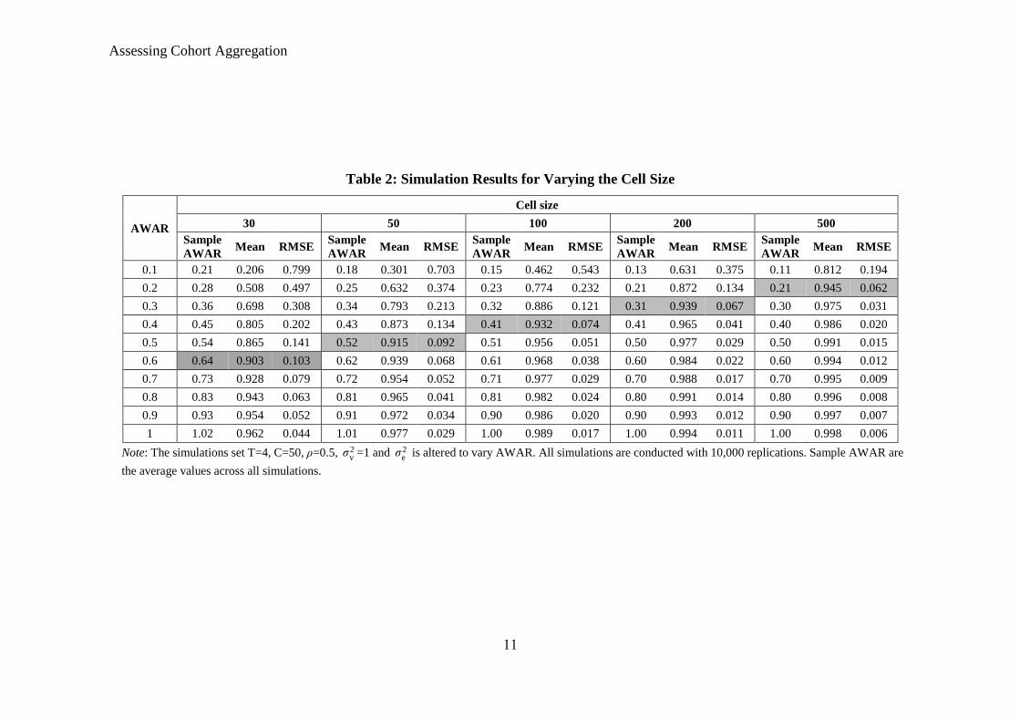
Table 2 shows the results for varying nc between 30 and 500 over different AWAR
values, where the latter is altered by just changing 2
eσ while keeping 2
vσ =1 and =0.5.
As predicted, the sampling error bias falls as AWAR increases for each cell size and
the reverse is also true, with the bias falling as cell size increases for each AWAR value.
If we assume estimates have sufficiently low bias to be considered accurate when the
bias is less than 10%, then the highlighted cells give an indication of the minimum
AWAR value required for accurate estimates for different cell sizes. One sees that cell
size of 30 can be accurate if AWAR is over 0.6 (0.64 for sample AWAR) but may not
be accurate even with cell size of 500 if AWAR is close to 0.1, showing the large impact
of AWAR on required cell size. Thus it is possible that creating more cohorts may lead
to less biased estimates even if cell sizes fall tenfold or more as long as AWAR
increases sufficiently. How much AWAR actually varies in empirical applications will
be demonstrated later, where we show that AWAR can lie between 0.1 and 0.6
depending on the cohort aggregation method used.
Assessing Cohort Aggregation
11
Table 2: Simulation Results for Varying the Cell Size
AWAR
Cell size
30 50 100 200 500
Sample
AWAR Mean RMSE
Sample
AWAR Mean RMSE
Sample
AWAR Mean RMSE
Sample
AWAR Mean RMSE
Sample
AWAR Mean RMSE
0.1 0.21 0.206 0.799 0.18 0.301 0.703 0.15 0.462 0.543 0.13 0.631 0.375 0.11 0.812 0.194
0.2 0.28 0.508 0.497 0.25 0.632 0.374 0.23 0.774 0.232 0.21 0.872 0.134 0.21 0.945 0.062
0.3 0.36 0.698 0.308 0.34 0.793 0.213 0.32 0.886 0.121 0.31 0.939 0.067 0.30 0.975 0.031
0.4 0.45 0.805 0.202 0.43 0.873 0.134 0.41 0.932 0.074 0.41 0.965 0.041 0.40 0.986 0.020
0.5 0.54 0.865 0.141 0.52 0.915 0.092 0.51 0.956 0.051 0.50 0.977 0.029 0.50 0.991 0.015
0.6 0.64 0.903 0.103 0.62 0.939 0.068 0.61 0.968 0.038 0.60 0.984 0.022 0.60 0.994 0.012
0.7 0.73 0.928 0.079 0.72 0.954 0.052 0.71 0.977 0.029 0.70 0.988 0.017 0.70 0.995 0.009
0.8 0.83 0.943 0.063 0.81 0.965 0.041 0.81 0.982 0.024 0.80 0.991 0.014 0.80 0.996 0.008
0.9 0.93 0.954 0.052 0.91 0.972 0.034 0.90 0.986 0.020 0.90 0.993 0.012 0.90 0.997 0.007
1 1.02 0.962 0.044 1.01 0.977 0.029 1.00 0.989 0.017 1.00 0.994 0.011 1.00 0.998 0.006
Note: The simulations set T=4, C=50, ρ=0.5, 2vσ =1 and 2
eσ is altered to vary AWAR. All simulations are conducted with 10,000 replications. Sample AWAR are
the average values across all simulations.
Assessing Cohort Aggregation
12
The results in Table 2 are presented to highlight the importance of cohort variation
when considering cell size. They are not to be interpreted as cell size and AWAR
combinations to use in practice. This is because the results are only robust to varying
the number of cohorts and to varying AWAR by changing 2
vσ rather than 2
eσ (although
the latter part shows that only the ratio of the two variances matters for addressing bias
and not their individual magnitudes). These results are not robust to changes in T, with
larger T reducing the required AWAR for each cell size. The results are also generally
not robust across the values of unless T is around 4 or 5. To avoid the cumbersome
process of having to calculate all the bias minimising combinations of cell size and
AWAR across all potential values of T and that one may encounter empirically, we
collapse AWAR and cell size into a single metric called CAWAR, cell size adjusted
AWAR.
2.4 Deriving and testing CAWAR
Recall that in (7) for AWAR the denominator is the variance across individuals within
a cohort ( 2
vσ ). This is not the same as the sampling error variance, 2w , identified as the
other factor alongside 1w that is important for determining the bias of pseudo-panel
estimates. To capture sampling error fully, one must incorporate cell size alongside 2
vσ
as shown in (4). Combining (4) and (7) we can derive CAWAR as (12) below, which
fully accounts for sampling error. The same proxies can be used as before as CAWAR
is equivalent to the square of AWAR multiplied by cell size. We use the square of
AWAR as it is not necessary to rescale using standard deviations.
2
2
1
2
2
e
2
2
)1( (7) From ,(4) From
vvc
v
σ
w
σ
σ
n
σ w
(AWAR))1(
CAWAR 2
2
2
1
2
2
ec
v
c nσ
nw
w
σ
(12)
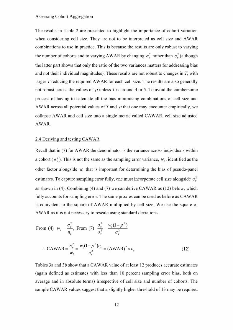
Tables 3a and 3b show that a CAWAR value of at least 12 produces accurate estimates
(again defined as estimates with less than 10 percent sampling error bias, both on
average and in absolute terms) irrespective of cell size and number of cohorts. The
sample CAWAR values suggest that a slightly higher threshold of 13 may be required
Assessing Cohort Aggregation
13
in actual applications using the proxies identified. These results are robust to different
absolute magnitudes of 2
eσ and 2
vσ , with only their ratio being of importance.
Table 3a: Varying Cell Size for CAWAR
Cell Size CAWAR of 12
Sample
CAWAR
Mean RMSE
30 13.39 0.912 0.095
50 13.27 0.912 0.095
100 13.21 0.912 0.094
150 13.18 0.911 0.095
200 13.17 0.912 0.095
250 13.16 0.912 0.094
500 13.16 0.911 0.095
1000 13.15 0.912 0.095
Note: The simulations set T=4, C=50, ρ=0.5, 2vσ =1 and 2
eσ is altered
to keep CAWAR=12 while nc changes. All simulations are conducted
with 10,000 replications.
Table 3b: Varying the Number of Cohorts for CAWAR
Number of
Cohorts
CAWAR of 12
Sample
CAWAR
Mean RMSE
20 13.13 0.912 0.105
50 13.29 0.911 0.095
100 13.31 0.912 0.092
200 13.35 0.912 0.090
500 13.37 0.912 0.089
Note: The simulations set T=4, nc=50, ρ=0.5, 2vσ =1 and 2
eσ =0.24
CAWAR. All simulations are conducted with 10,000 replications.
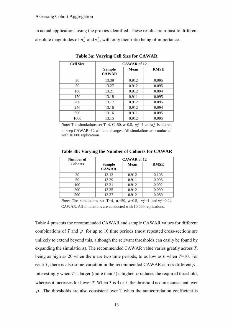
Table 4 presents the recommended CAWAR and sample CAWAR values for different
combinations of T and for up to 10 time periods (most repeated cross-sections are
unlikely to extend beyond this, although the relevant thresholds can easily be found by
expanding the simulations). The recommended CAWAR value varies greatly across T;
being as high as 20 when there are two time periods, to as low as 6 when T=10. For
each T, there is also some variation in the recommended CAWAR across different .
Interestingly when T is larger (more than 5) a higher reduces the required threshold,
whereas it increases for lower T. When T is 4 or 5, the threshold is quite consistent over
. The thresholds are also consistent over T when the autocorrelation coefficient is
Assessing Cohort Aggregation
14
lower than 0.4, especially when T≥4 the recommended threshold remains at 10 (11
using Sample CAWAR).
Table 4: CAWAR Thresholds for Different Timer Periods
ρ
2 Time Periods 3 Time Periods
CAWAR Sample
CAWAR
Mean RMSE CAWAR Sample
CAWAR
Mean RMSE
0 14 14.87 0.933 0.085 12 12.99 0.923 0.086
0.2 14 14.83 0.923 0.096 12 13.06 0.915 0.094
0.4 18 18.79 0.928 0.090 12 13.13 0.907 0.103
0.6 20 20.75 0.926 0.092 14 15.28 0.913 0.096
0.9 20 22.14 0.914 0.105 14 15.70 0.906 0.104
ρ
4 Time Periods 5 Time Periods
CAWAR Sample
CAWAR
Mean RMSE CAWAR Sample
CAWAR
Mean RMSE
0 10 11.05 0.910 0.097 10 11.08 0.909 0.096
0.2 10 11.08 0.901 0.105 10 11.11 0.904 0.101
0.4 10 11.18 0.898 0.109 10 11.21 0.902 0.103
0.6 12 13.39 0.911 0.096 10 11.40 0.902 0.102
0.9 12 13.76 0.908 0.098 10 11.83 0.906 0.099
ρ
8 Time Periods 10 Time Periods
CAWAR Sample
CAWAR
Mean RMSE CAWAR Sample
CAWAR
Mean RMSE
0 10 11.08 0.909 0.094 10 11.08 0.909 0.093
0.2 10 11.11 0.907 0.095 10 11.13 0.908 0.094
0.4 10 11.22 0.910 0.093 10 11.24 0.912 0.090
0.6 8 9.40 0.897 0.106 8 9.40 0.903 0.099
0.9 8 9.85 0.916 0.087 6 7.85 0.904 0.098
Note: The simulations set nc=50, C=50, 2vσ =1 and 2
eσ is altered to vary CAWAR. All simulations
are conducted with 10,000 replications.
Assessing Cohort Aggregation
15
3. Aggregation Bias
The main concern in estimation of pseudo-panels is bias arising from sampling error.
CAWAR, by combining both the cell size and cohort level variation, is a useful
practical measure for assessing and limiting the likelihood of such bias, something that
is lacking in the literature. However, sampling error bias may not be the only source of
bias arising from the cohort grouping process. There may be aggregation bias, which
arises when moving from the individual to the cohort level, potentially due to the loss
of variation in the cohort level data or the existence of non-linearities that are difficult
to capture using cohort averages. Pseudo-panels were initially used to estimate life-
cycle models of consumption and labour supply, where the unit of analysis was the age-
cohort itself (Table 1b), hence aggregation bias was not a concern. Applications in other
fields, particularly development, are interested mainly at household or individual level
analysis. Aggregation bias now becomes a concern as cohort panels are interpreted as
if they contain individual level data. There is awareness of this issue and pseudo-panel
studies in development economics (Table 1a) generally have larger c and use more
cohort selection variables than those used to estimate life-cycle models (Table 1b). It
is difficult to know whether this sufficiently addresses aggregation bias as the literature
has mostly neglected such concerns.
3.1 Separating Aggregation and Sampling Error
Aggregation bias is likely to be related to sampling error bias as 1w , 2
vσ , and time
variation are also linked to aggregation bias. Larger 1w and time variation indicates the
cohort means capture more of the distribution of the underlying individual level data,
while smaller 2
vσ ensures groups are more representative of their underlying sub-
populations as more homogenous individuals are grouped together. It therefore may be
difficult to disentangle sampling error from aggregation bias. Nevertheless, it is
necessary to do so as the presence of the latter calls into question whether pseudo-
panels can be analysed as if they are genuine individual-level panel estimates, as many
existing studies do.
Bias from aggregation and sampling error can be separated by estimating pseudo-
panels using panel data. Sampling error bias arises from the fact that ct is not constant
Assessing Cohort Aggregation
16
over time as the individuals in a cohort change over time when using RCS data.
However, when panel data are used the individuals grouped into cohorts are fixed over
time, thus ct is also fixed irrespective of cell size. As a result, we can adjust the number
of cohorts which captures effects of aggregation without affecting sampling error.
Using the panel fixed effects estimator, the ‘true’ coefficients can be estimated and
compared to the pseudo-panel estimates, where the difference can be thought of as the
bias from aggregation. This assumes that the panel estimates are the true values, which
may not be true due to concerns regarding attrition and measurement error, which will
be discussed later. If pseudo-panel estimates are all similar to each other and to the
panel estimates, aggregation is not a concern and the focus of constructing cohorts
should be mainly on addressing sampling error.
3.2 Data and Estimation
The dataset we use to investigate aggregation bias is the Uganda National Panel
Surveys (UNPS), using the four waves - 2005/06, 2009/10, 2010/2011 and 2011/2012.
The original 2005/06 data is taken from the Uganda National Household Survey which
contained a nationally representative sample of about 7,400 households. The panel is
constructed by re-interviewing 3,123 households from 322 of the original 783
enumeration areas located all over the country. As not all households were able to be
re-interviewed there is some attrition over the waves. The dataset contains detailed
information on household consumption, income, wealth, labour market activities as
well as information on the characteristics of individuals in the household such as their
age and education level. The surveys are consistent with LSMS, so are similar to survey
data available for other developing countries (the variables and the methods used to
construct cohorts can be replicated for other countries with similar data).
We estimate a model of household welfare, measured by the natural logarithm of
monthly household consumption per adult equivalent member (labelled lcons),
following Deaton and Zaidi (2002). This model is chosen because it is a useful baseline
for many empirical studies using such household data and fixed effects are likely to be
present due to unobserved time invariant factors like preferences, the intra-household
bargaining process, and innate characteristics of household members. The estimation
Assessing Cohort Aggregation
17
model is shown below and is a general model of household consumption, similar to
Glewwe (1991) and Appleton (1996) for example:
sec
(13) ender ocation
it1211
1098
2
765
4321
efftorregion
gleducationageage
lcons
ti
it
remittance
lnremit secondary ltotassetHHsize
Explanatory variables capture household characteristics; the number of household
members (HHsize), gender of household head, as well as their age and education level
(split into none, primary or post-primary). Income and assets variables are captured by
the main sector of employment of the household head (sector), a dummy for whether
they also engage in some secondary occupation (secondary), a dummy for whether the
household received any remittances in the last year (remittance) as well as the log of
the amount received (lnremit), and the log of total assets owned by the household
(ltotasset). Geographic characteristics are captured by the region the household is from
and whether it is based in an urban or rural location (location). Individual effects (𝑓𝑖)
and time effects (𝑓𝑡) are also included. The variables highlighted in bold are the ones
of interest as they vary across time and thus are not factored out by the inclusion of
fixed effects; OLS uses all the explanatory variables whereas fixed effects includes
only the ones in bold. Another reason for focusing only on these variables is because
the other variables will be used to construct cohorts and would have to be excluded
from the pseudo-panel regressions. Hence the pseudo-panel version of the model is:
(14)
ct5
4321
eff
lcons
tc
ct
remittance
lnremit secondary ltotassetHHsize
We construct cohorts using variables that are widely available and relevant to other
researchers using similar LSMS data to make our findings as general as possible.
Important conditions for construction variables are that they are time invariant,
exogenous and observed for all households in the sample. We use five variables
commonly used in the literature to construct cohorts: the age of the household head,
their gender, their education level, the region the household is from and whether it is in
a rural or urban location. We exclude the use of socioeconomic variables as these are
likely to be endogenous and many households change categories over time, particularly
Assessing Cohort Aggregation
18
when looking over a long time period. We exclude ethnicity because it is not highly
relevant in Uganda (but may be for other countries). Various age bands have been used
in the literature, the most common being 5 year bands, however others have also used
1 year, 2 year and 10 year bands. We construct cohorts based on 2 year, 5 year, 10 year
and 17 year age bands, giving us a good range to assess aggregation. Furthermore, we
only use households whose head is aged 18-67 at the time of each survey.
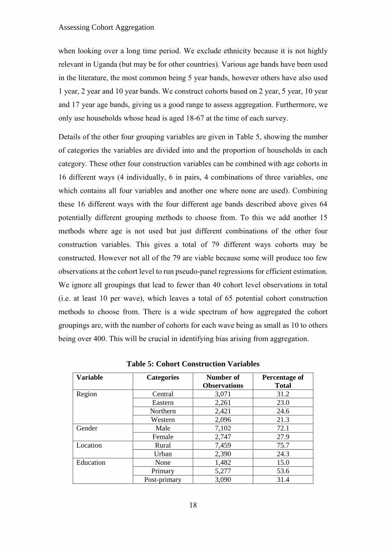
Details of the other four grouping variables are given in Table 5, showing the number
of categories the variables are divided into and the proportion of households in each
category. These other four construction variables can be combined with age cohorts in
16 different ways (4 individually, 6 in pairs, 4 combinations of three variables, one
which contains all four variables and another one where none are used). Combining
these 16 different ways with the four different age bands described above gives 64
potentially different grouping methods to choose from. To this we add another 15
methods where age is not used but just different combinations of the other four
construction variables. This gives a total of 79 different ways cohorts may be
constructed. However not all of the 79 are viable because some will produce too few
observations at the cohort level to run pseudo-panel regressions for efficient estimation.
We ignore all groupings that lead to fewer than 40 cohort level observations in total
(i.e. at least 10 per wave), which leaves a total of 65 potential cohort construction
methods to choose from. There is a wide spectrum of how aggregated the cohort
groupings are, with the number of cohorts for each wave being as small as 10 to others
being over 400. This will be crucial in identifying bias arising from aggregation.
Table 5: Cohort Construction Variables
Variable Categories Number of
Observations
Percentage of
Total
Region Central 3,071 31.2
Eastern 2,261 23.0
Northern 2,421 24.6
Western 2,096 21.3
Gender Male 7,102 72.1
Female 2,747 27.9
Location Rural 7,459 75.7
Urban 2,390 24.3
Education None 1,482 15.0
Primary 5,277 53.6
Post-primary 3,090 31.4
Assessing Cohort Aggregation
19
Due to attrition and household members splitting off to form news ones, which the
UNPS also tracks, only around a half of all the households appear in all four waves
(1,711 out of 3,404). Although using just these households would completely mitigate
the sampling error problem and isolate aggregation bias, it may lead to bias from
attrition both in the panel and pseudo-panel estimates. To limit this, we estimate using
the full sample of households (where around three quarters of households appear in at
least two waves), meaning sampling error is not fully addressed. We include the results
using the fully balanced panel in Appendix A and they are largely identical. We
estimate equation (14) with all 65 cohort specifications using EWALD with weights
based on the square-root of cell size to address heteroscedasticity. We also drop all
cohorts that contain less than two households to ensure we retain the grouped element
and pseudo-panel results are not dominated by cohorts which essentially identify a
single household thus making it more akin to a genuine panel.
3.3 Results
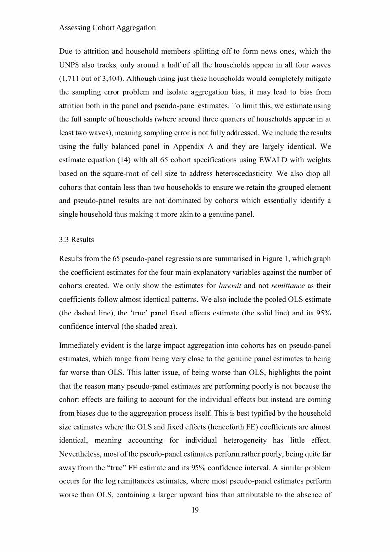
Results from the 65 pseudo-panel regressions are summarised in Figure 1, which graph
the coefficient estimates for the four main explanatory variables against the number of
cohorts created. We only show the estimates for lnremit and not remittance as their
coefficients follow almost identical patterns. We also include the pooled OLS estimate
(the dashed line), the ‘true’ panel fixed effects estimate (the solid line) and its 95%
confidence interval (the shaded area).
Immediately evident is the large impact aggregation into cohorts has on pseudo-panel
estimates, which range from being very close to the genuine panel estimates to being
far worse than OLS. This latter issue, of being worse than OLS, highlights the point
that the reason many pseudo-panel estimates are performing poorly is not because the
cohort effects are failing to account for the individual effects but instead are coming
from biases due to the aggregation process itself. This is best typified by the household
size estimates where the OLS and fixed effects (henceforth FE) coefficients are almost
identical, meaning accounting for individual heterogeneity has little effect.
Nevertheless, most of the pseudo-panel estimates perform rather poorly, being quite far
away from the “true” FE estimate and its 95% confidence interval. A similar problem
occurs for the log remittances estimates, where most pseudo-panel estimates perform
worse than OLS, containing a larger upward bias than attributable to the absence of
Assessing Cohort Aggregation
20
fixed effects. Figure A1 in Appendix A shows the equivalent results for the fully
balanced panel, which are qualitatively similar.
Figure 1: Pseudo-panel estimates of the 65 cohort construction methods
Note: The scatter plots are the pseudo-panel estimates of equation (14) obtained by the 65 different cohort
construction methods. The solid line shows the “true” fixed effects estimates of equation (13) for just
the main variables in bold and excluding the time invariant additional controls. The grey area is its 95%
confidence interval. The dashed line shows the pooled OLS estimates of equation (13), including all the
additional controls but not accounting for the individual effects. Both the OLS and fixed effects estimates
are based on the household level panel data with the data trimmed at the 1st and 99th percentiles.
For log total assets, accounting for unobserved heterogeneity is necessary as the FE
estimate is significantly smaller in magnitude than the OLS estimate. The pseudo-panel
estimates generally outperform the OLS estimates, as the inclusion of cohort effects
picks up the unobserved heterogeneity, and many of the estimates are very close to the
“true” FE values. However, a significant proportion offer little improvement over OLS
or are worse, showing that a reduction in bias from the inclusion of cohort effects can
be offset by increased bias coming from aggregation. One can see a similar pattern for
secondary occupation, for which including fixed effects is essential: OLS indicates a
negative and significant coefficient whereas FE results in a positive and significant
coefficient. The pseudo-panel estimates pick up the effect of fixed effects, with the vast
-.12
-.1
-.08
-.06
-.04
Coeffic
ien
t E
stim
ate
0 100 200 300 400Number of Cohorts
Household Size
0.0
5.1
.15
.2.2
5C
oeffic
ien
t E
stim
ate
0 100 200 300 400Number of Cohorts
Log Total Assets
-.4
-.2
0.2
.4C
oeff
icie
nt E
stim
ate
0 100 200 300 400Number of Cohorts
Secondary Occupation-.
10
.1.2
.3.4
Coeff
icie
nt E
stim
ate
0 100 200 300 400Number of Cohorts
Log Remittance
Assessing Cohort Aggregation
21
majority of coefficient estimates being positive, although many are still highly biased
(the magnitudes are often five to ten times larger than the “true” FE coefficient). It also
demonstrates just how much impact cohort construction has on the coefficient
estimates, which can vary from being smaller than -0.3 to larger than +0.4 even though
the OLS and FE estimates are -0.02 and +0.05 respectively.
Estimates of all four variables improve as the number of cohort increases, consistent
with bias from aggregation. In addition, for all variables except log remittance,
aggregation does not affect the bias in a specific way: the pseudo-panel estimates are
just as likely to be biased upwards as downwards. When the number of cohorts are low
estimates appear random, often varying with a large distribution around a mean that is
close to the ‘true’ fixed effects coefficient. When the number of cohorts is larger, at
around 150-200 or more, pseudo-panel estimates generally converge to the ‘true’
coefficients. Consequently, pseudo-panel estimates can suffer from substantial
aggregation bias, which in some cases can be so large that pooled OLS is a better
alternative. However, cohorts can be constructed in a way to limit this and achieve
estimates similar to panel fixed effects.
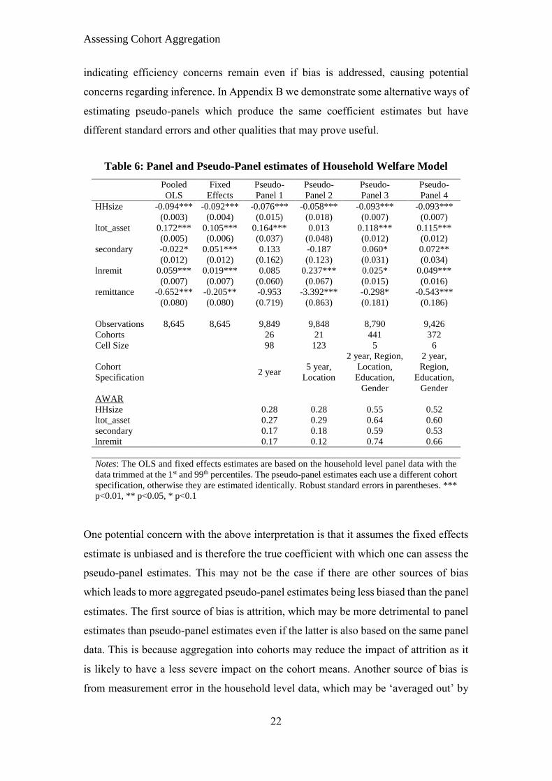
Table 6 contains a few of the pseudo-panel results, as well as the OLS and FE estimates,
to demonstrate this. The third and fourth columns give examples of poor aggregation
which results in unstable and inaccurate coefficient estimates, whereas the final two
columns give examples of the opposite. The former pair are based on common cohort
aggregation methods that can be found in the literature; one uses just 2-year age cohorts
(similar to Warunsiri and McNown, 2010) and the other uses 5-year age bands
combined with a geographic variable (location in our case). Both have cell sizes of
around 100 or more, which is commonly thought as being sufficient to ensure accurate
estimates. This calls into question studies that use similar aggregation methods and
interpret results at the household or individual level, where the low c cause both bias
and efficiency issues. Whether this can be addressed by ensuring c is more than 150-
200, like our results imply, will be addressed later. The last two columns show that
aggregation bias can be addressed using commonly available construction variables,
producing pseudo panel estimates that are similar in terms of size and significance to
panel results. Nevertheless, these estimates, which have more than 300 cohorts in each
time period, have standard errors that are far larger than the FE and OLS, estimates
Assessing Cohort Aggregation
22
indicating efficiency concerns remain even if bias is addressed, causing potential
concerns regarding inference. In Appendix B we demonstrate some alternative ways of
estimating pseudo-panels which produce the same coefficient estimates but have
different standard errors and other qualities that may prove useful.
Table 6: Panel and Pseudo-Panel estimates of Household Welfare Model
Pooled
OLS
Fixed
Effects
Pseudo-
Panel 1
Pseudo-
Panel 2
Pseudo-
Panel 3
Pseudo-
Panel 4
HHsize -0.094*** -0.092*** -0.076*** -0.058*** -0.093*** -0.093***
(0.003) (0.004) (0.015) (0.018) (0.007) (0.007)
ltot_asset 0.172*** 0.105*** 0.164*** 0.013 0.118*** 0.115***
(0.005) (0.006) (0.037) (0.048) (0.012) (0.012)
secondary -0.022* 0.051*** 0.133 -0.187 0.060* 0.072**
(0.012) (0.012) (0.162) (0.123) (0.031) (0.034)
lnremit 0.059*** 0.019*** 0.085 0.237*** 0.025* 0.049***
(0.007) (0.007) (0.060) (0.067) (0.015) (0.016)
remittance -0.652*** -0.205** -0.953 -3.392*** -0.298* -0.543***
(0.080) (0.080) (0.719) (0.863) (0.181) (0.186)
Observations 8,645 8,645 9,849 9,848 8,790 9,426
Cohorts 26 21 441 372
Cell Size 98 123 5 6
Cohort
Specification 2 year
5 year,
Location
2 year, Region,
Location,
Education,
Gender
2 year,
Region,
Education,
Gender
AWAR
HHsize 0.28 0.28 0.55 0.52
ltot_asset 0.27 0.29 0.64 0.60
secondary 0.17 0.18 0.59 0.53
lnremit 0.17 0.12 0.74 0.66
Notes: The OLS and fixed effects estimates are based on the household level panel data with the
data trimmed at the 1st and 99th percentiles. The pseudo-panel estimates each use a different cohort
specification, otherwise they are estimated identically. Robust standard errors in parentheses. ***
p<0.01, ** p<0.05, * p<0.1
One potential concern with the above interpretation is that it assumes the fixed effects
estimate is unbiased and is therefore the true coefficient with which one can assess the
pseudo-panel estimates. This may not be the case if there are other sources of bias
which leads to more aggregated pseudo-panel estimates being less biased than the panel
estimates. The first source of bias is attrition, which may be more detrimental to panel
estimates than pseudo-panel estimates even if the latter is also based on the same panel
data. This is because aggregation into cohorts may reduce the impact of attrition as it
is likely to have a less severe impact on the cohort means. Another source of bias is
from measurement error in the household level data, which may be ‘averaged out’ by
Assessing Cohort Aggregation
23
using cohort means (Antman & McKenzie, 2007b). Constructing more aggregated
cohorts would reduce the bias arising from both these potential sources. However, as
the results show that estimates from more aggregated pseudo-panels vary greatly and
diverge from the fixed effects estimates in a non-systematic manner, we can be
confident that such additional biases do not play a big role and leave the main
conclusions regarding aggregation bias unchanged.
The previous section showed there was no specific cell size which sufficiently
addressed sampling error as it depends on the level of variation in the cohort data. For
similar reasons, it is unlikely that aggregation bias can be addressed by creating a
specific number of cohorts and instead the bias depends on how representative the
cohort level data are of the underlying households. The latter, to a certain degree, will
be related to the number of cohorts and hence it may appear that aggregation bias can
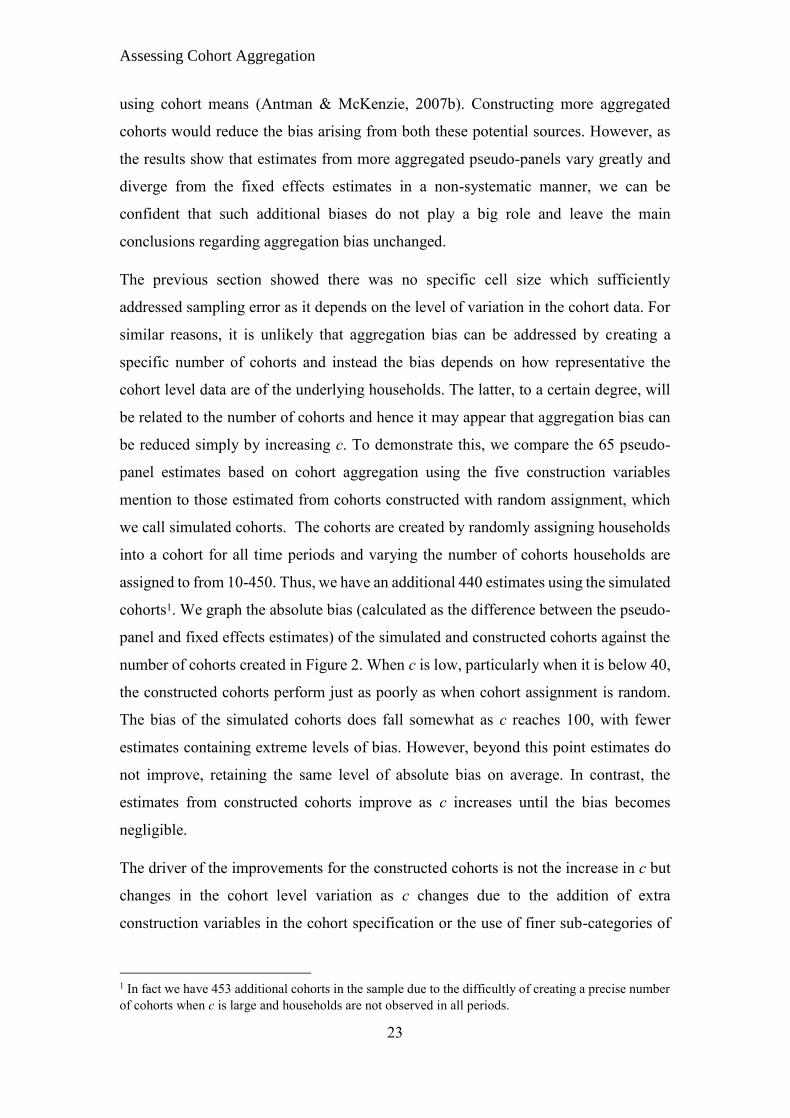
be reduced simply by increasing c. To demonstrate this, we compare the 65 pseudo-
panel estimates based on cohort aggregation using the five construction variables
mention to those estimated from cohorts constructed with random assignment, which
we call simulated cohorts. The cohorts are created by randomly assigning households
into a cohort for all time periods and varying the number of cohorts households are
assigned to from 10-450. Thus, we have an additional 440 estimates using the simulated
cohorts1. We graph the absolute bias (calculated as the difference between the pseudo-
panel and fixed effects estimates) of the simulated and constructed cohorts against the
number of cohorts created in Figure 2. When c is low, particularly when it is below 40,
the constructed cohorts perform just as poorly as when cohort assignment is random.
The bias of the simulated cohorts does fall somewhat as c reaches 100, with fewer
estimates containing extreme levels of bias. However, beyond this point estimates do
not improve, retaining the same level of absolute bias on average. In contrast, the
estimates from constructed cohorts improve as c increases until the bias becomes
negligible.
The driver of the improvements for the constructed cohorts is not the increase in c but
changes in the cohort level variation as c changes due to the addition of extra
construction variables in the cohort specification or the use of finer sub-categories of
1 In fact we have 453 additional cohorts in the sample due to the difficultly of creating a precise number
of cohorts when c is large and households are not observed in all periods.
Assessing Cohort Aggregation
24
age. Previously we discussed the link between aggregation bias and sampling error,
particularly the link with 1w , 2 vσ , and time variation. As these three types or variation
are combined to form the AWAR metric, AWAR can potentially be used to assess the
likelihood of aggregation bias. CAWAR is unlikely to be suitable as it allows larger
cell size to offset low variation, which is justifiable for sampling error but not
aggregation.
Figure 2: Bias of constructed and simulated cohorts
Notes: The y-axis calculates the absolute different between the pseudo-panel estimate and the FE
estimate. Constructed cohorts refers to the 65 cohorts constructed where assignment is based on
construction variables from the dataset, while simulated cohorts refers to cohorts created by random
assignment.
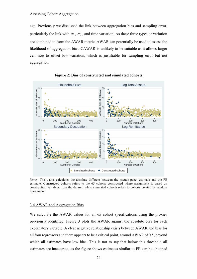
3.4 AWAR and Aggregation Bias
We calculate the AWAR values for all 65 cohort specifications using the proxies
previously identified. Figure 3 plots the AWAR against the absolute bias for each
explanatory variable. A clear negative relationship exists between AWAR and bias for
all four regressors and there appears to be a critical point, around AWAR of 0.5, beyond
which all estimates have low bias. This is not to say that below this threshold all
estimates are inaccurate, as the figure shows estimates similar to FE can be obtained
0.0
5.1
.15
Absolu
te B
ias o
f E
stim
ate
0 100 200 300 400Number of Cohorts
Household Size
0.0
5.1
.15
Absolu
te B
ias o
f E
stim
ate
0 100 200 300 400Number of Cohorts
Log Total Assets
0.2
.4.6
Absolu
te B
ias o
f E
stim
ate
0 100 200 300 400Number of Cohorts
Secondary Occupation
0.1
.2.3
.4A
bsolu
te B
ias o
f E
stim
ate
0 100 200 300 400Number of Cohorts
Log Remittance
Simulated cohorts Constructed cohorts
Assessing Cohort Aggregation
25
even at low AWAR. Instead the threshold ensures confidence that any estimate
produced will not suffer from substantial bias caused by the aggregation process. In
Table 6 we report the AWAR statistics for the four pseudo-panel regressions, showing
the link between AWAR and how well the panel estimates are replicated. Like the
estimates in the final two columns of Table 6, we find regressions where all explanatory
variables have AWAR of at least 0.5 generally produce estimates that improve on
pooled OLS and are similar to FE. In our application, only 4 of the 65 specifications
meet this condition, highlighting that this may be quite a strict condition to meet.
However, all the cohort specifications that failed to meet this condition generally have
one or more poorly estimated regressor, such that the OLS estimate is less biased.
Figure 3: AWAR and Estimation Bias
Notes: The y-axis is calculates the absolute different between the pseudo-panel estimate and the panel
fixed effects estimate.
Evidently, AWAR is a useful measure for assessing the potential for aggregation bias,
which we have shown can be rather large when estimating pseudo-panels. Whether the
critical value (AWAR of around 0.5) found in our empirical example can be used as a
general recommendation for applications in other studies is unclear. One reason to
believe they may be is because the threshold is stable across the four regressors which
0.0
1.0
2.0
3.0
4.0
5A
bsolu
te B
ias o
f E
stim
ate
0 .2 .4 .6 .8AWAR
Household Size
0.0
5.1
.15
Absolu
te B
ias o
f E
stim
ate
0 .2 .4 .6 .8AWAR
Log Total Assets
0.1
.2.3
.4A
bsolu
te B
ias o
f E
stim
ate
0 .2 .4 .6 .8AWAR
Secondary Occupation
0.1
.2.3
.4A
bsolu
te B
ias o
f E
stim
ate
0 .2 .4 .6 .8AWAR
Log Remittance
Assessing Cohort Aggregation
26
are vastly different in their nature; one is continuous, one truncated and the other two
are either categorical or binary. They all have different distributions but still require
similar AWAR values. The four regressors also capture different properties and
characteristics of households with little reason to suspect they are highly correlated
with each other or share similar correlations with the cohort construction variables.
Consequently, it is likely that similar thresholds would apply for other variables from
different datasets.
A greater concern is whether the thresholds change when moving from panel data to
repeated cross-sections. The within variation (which captures 2 vσ ) is unlikely to change
between the two types of data as the heterogeneity of households grouped into cohort
will not be affected. With panel data, as cohort membership is constant, the cohort
means are likely to be more highly correlated across time than with data that has
different individuals in each cross-section. Thus, panel data will have less time
variation (higher ) and potentially lower across variation (lower 1 w ) as the latter picks
up some time variation as well as cross-sectional variation. Consequently, repeated
cross-sections would generally have higher AWAR values (as is higher and is
lower) than panel data. This could affect the thresholds we find if panel data naturally
has lower AWAR than RCS irrespective of aggregation. We consider this in Appendix
C, where we re-estimate the above model using the same dataset, once again creating
the 65 cohort specifications but using just the first two waves. In Figure C2 we
randomly drop households so that each only appears once, hence getting rid of the panel
dimension, while in Figure C1 we retain the panel setting. The estimates in Figure C2
contain both aggregation and sampling error bias, while for those in Figure C1 the
sampling error is severely reduced due to the use of panel data. We find AWAR is
generally lower for panel data, but AWAR of 0.5 still seems a reasonable threshold for
RCS even though it is hard to assess aggregation bias due to the additional presence of
sampling error.
1w
Assessing Cohort Aggregation
27
4. Implementing AWAR and CAWAR
The two metrics developed help address different but connected sources of bias one
encounters when estimating pseudo-panels; sampling error and aggregation. The bias
from the latter can be so substantial that it negates any benefit of using pseudo-panels
over simple OLS. Hence, it is important to ensure the cohorts created have AWAR
close to 0.5 as well as meeting the required CAWAR value needed to limit sampling
error. Whether these thresholds are met in practice remains a concern, particularly as
so few cohort aggregation methods met the AWAR threshold in our empirical example.
We attempt to draw some inferences regarding the likelihood of other datasets meeting
our suggested criteria using results from our empirical application and the Monte Carlo
simulations for AWAR.
The results in the final two columns of Table 6 show that our dataset requires a large
number of cohorts in order to meet the AWAR threshold, such that average cell sizes
fall to as low as 5 or 6. Two other cohort specifications also meet the AWAR threshold
(not reported) but again they have cell sizes of 6 and 8 respectively. The AWAR
simulations in Table 2 suggest cell size needs to be at least 50, possibly 30, to avoid
sampling error bias if the data was repeated cross-sections2. The comparison of Figures
C1 and C2 shows that the same cohort aggregation process produced higher AWAR
for RCS than panel data. With actual RCS some of the more aggregate cohort
specifications (which have higher cell size) will meet the AWAR threshold. Even then,
they are unlikely to have cell sizes higher than 10-15. Therefore, the dataset would need
to be 3-5 times larger to obtain cell sizes needed to address sampling error while also
meeting the AWAR threshold for aggregation. Given our dataset has around 2,500
households in each wave, this implies RCS data may require at least 7,000 observations
in each wave to address both sources of bias. Many RCS datasets are large enough to
meet this condition, particularly those used in development economics. For example,
most studies in Table 1a have datasets with the required number of observation in each
wave. These calculations assume the cohort specifications and their respective AWAR
values taken from our empirical application is representative of other datasets. This is
2 The results in Table 2 are applicable to our empirical example as the simulations have the same T and
the results are robust for different values of ρ and c.
Assessing Cohort Aggregation
28
not necessarily true; the required number of observations will be lower if there is
greater correlation between the cohort construction variables and the explanatory
variables, while the reverse is also true. Nevertheless, it may still be a useful benchmark
for pseudo-panels with similar data.
5. Conclusion
Addressing sampling error is a crucial part of estimating pseudo-panel models but there
is little guidance and consensus regarding how this should be done. We create a
measure (called CAWAR), which combines the cell sizes created along with three
important sources of variation in the cohort data, to assess the likelihood of sampling
error. Using Monte Carlo simulations, we find critical values for the measure beyond
which sampling error bias is minimised. We also show that when pseudo-panels are
used to estimate individual level models they can suffer from substantial aggregation
bias. As aggregation and sampling error biases are related, a similar measure (called
AWAR) can be used to assess the former. Using panel data, we estimate pseudo-panels
to isolate aggregation bias and find recommended values for AWAR where this bias is
minimised.
Ensuring CAWAR and AWAR meet the recommended values should be the starting
point of validating pseudo-panel estimation, particularly for individual level models.
This can be quite a strict requirement that some datasets are unable to fulfil, implying
they may be unsuited to pseudo-panel estimation. It is therefore important to confirm
the veracity of these recommended values, particularly as CAWAR has only been
tested using simulations and AWAR using a panel dataset. The testing we have
conducted is suited to isolating the two different sources of bias, thus what is required
for future work is testing them in combination. One way to do this is using a large panel
data set where the “true” coefficient can be estimated using panel fixed effects. Then a
random subset of the population can be drawn for each time period to create a repeated
cross-section with which pseudo-panels can be estimated. The dataset would need to
be large enough that the subsets in each time period have enough observations to
produce AWAR and CAWAR that meets the recommended values.
Assessing Cohort Aggregation
29
Another possibility would be to use a more complex Monte Carlo setup where the
individual level data is first generated and then grouped into cohorts using construction
variables that have varying degrees of correlation with the explanatory variables, in
order to capture a more realistic aggregation process. This allows the simulations to
address both sampling error and aggregation, in contrast to our simulations that focus
exclusively on the former. One could also test if the recommended thresholds change
for different models as application of pseudo-panels has moved beyond the simple
linear fixed effects model considered here. Some pertinent examples are nonlinear
models (particularly ones with a binary response variable), dynamic models, and ones
with parameter heterogeneity.
One final avenue for future work is combining different datasets (whether they are RCS
or panel) by matching on cohorts. If aggregation has been fully addressed, cohorts can
be thought of as representative households and hence one may be able to combine data
from different surveys. For example, it may be possible to combine many of the
Demographic and Health Surveys with household income/expenditure surveys as long
as they share the same variables required for cohort construction. There are some
important concerns that arise from this, particularly regarding the sampling methods
used for the different surveys and the effect of having a different set of individuals not
just in each time period but also for different variables within a time period. However,
if such a merger is possible it would widen the scope of research and allow the
estimation of models not possible before.
Assessing Cohort Aggregation
30
References
Alessie, R., Devereux, M.P. and Weber, G., 1997. Intertemporal consumption, durables and
liquidity constraints: A cohort analysis. European Economic Review, 41, pp.37–59.
Angrist, J.D., 1991. Grouped-data estimation and testing in simple labor-supply models.
Journal of Econometrics, 47, pp.243–266.
Antman, F. and McKenzie, D., 2007a. Poverty traps and nonlinear income dynamics with
measurement error and individual heterogeneity. Journal of Development Studies, 43(6),
pp.1057–1083.
Antman, F. and McKenzie, D., 2007b. Earnings mobility and measurement error: A pseudo-
panel approach. Economic Development and Cultural Change, 56(1), pp.125–161.
Appleton, S., 1996. Women-headed households and household welfare: An empirical
deconstruction for Uganda. World Development, 24(12), pp.1811-1827.
Arestoff, F. and Djemai, E., 2016. Women’s Empowerment Across the Life Cycle and
Generations: Evidence from Sub-Saharan Africa. World Development, 87, pp.70-87.
Attanasio, O.P., Blow, L., Hamilton, R. and Leicester, A., 2009. Booms and busts:
Consumption, house prices and expectations. Economica, 76, pp.20–50.
Banks, J., Blundell, R. and Preston, I., 1994. Life-cycle expenditure allocations and the
consumption costs of children. European Economic Review, 38, pp.1391–1410.
Bedi, A.S., Kimalu, P. K., Manda, D.K. and Nafula, N., 2004. The decline in primary school
enrolment in Kenya. Journal of African Economies, 13(1), pp.1–43.
Bernard, J.T., Bolduc, D. and Yameogo, N.D., 2011. A pseudo-panel data model of household
electricity demand. Resource and Energy Economics, 33, pp.315–325.
Blundell, R., Browning, M. and Meghir, C., 1994. Consumer demand and the life-cycle
allocation of household expenditures. Review of Economic Studies, (61), pp.57–80.
Blundell, R., Duncan, A. and Meghir, C., 1998. Estimating labour supply responses using tax
reforms. Econometrica, 66(4), pp.827–861.
Browning, M., Deaton, A. and Irish, M., 1985. A profitable approach to labor supply and
commodity demands over the life-cycle. Econometrica, 53(3), pp.503–543.
Campbell, J.Y. and Cocco, J.F., 2007. How do house prices affect consumption? Evidence
from micro data. Journal of Monetary Economics, 54, pp.591–621.
Christiaensen, L.J. and Subbarao, K., 2005. Towards an understanding of household
vulnerability in rural Kenya. Journal of African Economies, 14(4), pp.520–558.
Collado, M.D., 1998. Estimating binary choice models from cohort data. Investigaciones
Economicas, 22(2), pp.259-76.
Cuesta, J., Ñopo, H. and Pizzolitto, G., 2011. Using pseudo-panels to measure income mobility
in Latin America. Review of Income and Wealth, 57(2), pp.224–246.
Dargay, J.M., 2002. Determinants of car ownership in rural and urban areas: A pseudo-panel
analysis. Transportation Research Part E: Logistics and Transportation Review, 38,
pp.351–366.
Dargay, J.M. and Vythoulkas, P.C., 1999. Estimation of a dynamic car ownership model: A
pseudo-panel approach. Journal of Transport Economics and Policy, 33(3), pp.287–302.
Deaton, A., 1985. Panel data from time series of cross-sections. Journal of Econometrics, 30,
pp.109–126.
Deaton, A. and Paxson, C., 1994. Intertemporal choice and inequality. Journal of Political
Economy, 102(3), pp.437–467.
Deaton, A. and Zaidi, S., 2002. Guidelines for constructing consumption aggregates for
welfare analysis (Vol. 135). World Bank Publications.
Assessing Cohort Aggregation
31
Devereux, P.J., 2007a. Improved errors-in-variables estimators for grouped data. Journal of
Business & Economic Statistics, 25(3), pp.278–287.
Devereux, P.J., 2007b. Small-sample bias in synthetic cohort models of labour supply. Journal
of Applied Econometrics, 22, pp.839–848.
Échevin, D., 2013. Measuring vulnerability to asset-poverty in Sub-Saharan Africa. World
Development, 46, pp.211–222.
Fernandez-Villaverde, J. and Krueger, D., 2007. Consumption over the life cycle: facts from
consumer expenditure survey data. Review of Economics and Statistics, 89(3), pp.552–565.
Fulford, S., 2014. Returns to education in India. World Development, 59, pp.434–450.
Fuller, W.A., 1975. Regression analysis for sample survey, Sankhya: The Indian Journal of
Statistics, C37, pp.117-132
Fuller, W.A., 1981. Measurement error models (Department of Statistics, Iowa State
University, Ames, IA).
Gardes, F., Duncan, G., Gaubert, P., Gurgand, M. and Starzec, C., 2005. Panel and pseudo-
panel estimation of cross-sectional and time series elasticities of food consumption: The
case of American and Polish data. Journal of Business & Economic Statistics, 23(2),
pp.242–253.
Gassner, K., 1998. An estimation of UK telephone access demand using pseudo-panel data.
Utilities Policy, 7(3), pp.143–154.
Girma, S., 2000. A quasi-differencing approach to dynamic modelling from a time series of
independent cross-sections. Journal of Econometrics, 98, pp.365–383.
Glewwe, P., 1991. Investigating the Determinants of Household Welfare in the Côte d'Ivoire.
Journal of Development Economics. 35: 307-37.
Gómez Soler, S.C., 2016. Educational achievement at schools: Assessing the effect of the civil
conflict using a pseudo-panel of schools. International Journal of Educational
Development, 49, pp.91–106.
Güell, M. and Hu, L., 2006. Estimating the probability of leaving unemployment using
uncompleted spells from repeated cross-section data. Journal of Econometrics, 133(1),
pp.307–341.
Heshmati, A. and Kumbhakar, S.C., 1997. Estimation of technical efficiency in Swedish crops
farms: a pseudo panel data approach. Journal of Agricultural Economics, 48(1), pp.22–37.
Himaz, R. and Aturupane, H., 2016. Returns to education in Sri Lanka: A pseudo-panel
approach. Education Economics, 24(3), pp.300–311.
Imai, K.S., Annim, S.K., Kulkarni, V.S. and Gaiha, R., 2014. Women’s empowerment and
prevalence of stunted and underweight children in rural India. World Development, 62,
pp.88–105.
Jiang, S.S. and Dunn, L.F., 2013. New evidence on credit card borrowing and repayment
patterns. Economic Inquiry, 51(1), pp.394–407.
Juodis, A., 2017. Pseudo Panel Data Models with Cohort Interactive Effects. Journal of
Business & Economic Statistics
Kuha, J. and Temple, J., 2003. Covariate measurement error in quadratic regression.
International Statistical Review, 71(1), pp.131-150.
McKenzie, D.J., 2004. Asymptotic theory for heterogeneous dynamic pseudo-panels. Journal
of Econometrics, 120, pp.235–262.
Meng, Y., Brennan, A., Purshouse, R., Hill-McManus, D., Angus, C., Holmes, J. and Meier,
P.S., 2014. Estimation of own and cross price elasticities of alcohol demand in the UK - A
pseudo-panel approach using the Living Costs and Food Survey 2001-2009. Journal of
Health Economics, 34, pp.96–103.
Moffitt, R., 1993. Identification and estimation of dynamic models with a time series of
repeated cross-sections. Journal of Econometrics, 59, pp.99–123.
Assessing Cohort Aggregation
32
Nicita, A., 2009. The price effect of tariff liberalization: Measuring the impact on household
welfare. Journal of Development Economics, 89, pp.19–27.
Paul, C.J.M. and Nehring, R., 2005. Product diversification, production systems, and economic
performance in U.S. agricultural production. Journal of Econometrics, 126, pp.525–548.
Propper, C., Rees, H. and Green, K., 2001. The Demand for Private Medical Insurance in the
UK : A Cohort Analysis. The Economic Journal, 111(471), pp.180–200.
Rupert, P. and Zanella, G., 2015. Revisiting wage, easrnings, and hours profiles. Journal of
Monetary Economics, 72, pp.114–130.
Shimeles, A. and Ncube, M., 2015. The Making of the Middle-Class in Africa: Evidence from
DHS Data. Journal of Development Studies, 51(2), pp.178–193.
Sprietsma, M., 2012. Computers as pedagogical tools in Brazil: a pseudo-panel analysis.
Education Economics, 20(1), pp.19–32.
Verbeek, M., 2008. Pseudo Panels and Repeated Cross Sections. In: Matyas, L. and Sevestre,
P. eds. The Econometrics of Panel Data: Fundamental and Recent Development in Theory
and Practice Third Edition. Berlin: Springer, pp.369–383.
Verbeek, M. and Nijman, T., 1992. Can cohort data be treated as genuine panel data? Empirical
Economics, 17, pp.9–23.
Verbeek, M. and Nijman, T., 1993. Minimum MSE estimation of a regression model with fixed
effects from a series of cross-sections. Journal of Econometrics, 59, pp.125–136.
Verbeek, M. and Vella, F., 2005. Estimating Dynamic Models From Repeated Cross-Sections.
Journal of Econometrics, 127, pp.83–102.
Warunsiri, S. and McNown, R., 2010. The returns to education in Thailand: A pseudo-panel
approach. World Development, 38(11), pp.1616–1625.
Wolter, K.M. and Fuller, W.A., 1982. Estimation of the quadratic errors-in-variables model.
Biometrika, 69(1), pp.175-182.
Assessing Cohort Aggregation
33
Appendix A: Replication of Pseudo-Panel results using balanced panels
We reproduce all pseudo-panel results using just households observed in all four waves,
thus ensuring sampling error is eliminated as cohort membership is fixed. However,
this comes at the expense of potentially incurring attrition bias with just over half of all
households being in the balanced panel. Figure A1 and Table A1 shows that using
balanced panels does not affect the results in the main analysis. From Figure A1 (the
corollary to Figure 1), one sees that aggregation bias is still evident, with the pattern of
bias across the number of cohorts being largely the same. The balanced panel does
produce less biased estimates, with more appearing in the 95% confidence interval of
the ‘true’ coefficients, but the effect is small. Table A1 also produces similar results to
its counterpart (Table 6), particularly in terms of bias. However the examples which
meet the AWAR threshold have poor inference with some variables losing significance.
This is due to the loss of observations in the balanced panel, although the poor inference
can be addressed by using alternative estimation techniques discussed in Appendix B.
Figure A2 shows the relationship between AWAR and aggregation bias is also
unchanged.
Figure A1: Pseudo-Panel Estimates using Balanced Panels
Notes: Same as for Figure 1 but using balanced panels
-.1
-.05
0C
oeffic
ien
t E
stim
ate
0 100 200 300Number of Cohorts
Household Size
0.1
.2.3
Coeffic
ien
t E
stim
ate
0 100 200 300Number of Cohorts
Log Total Assets
-.4
-.2
0.2
.4.6
Coeff
icie
nt E
stim
ate
0 100 200 300Number of Cohorts
Secondary Occupation
0.1
.2.3
.4C
oeff
icie
nt E
stim
ate
0 100 200 300Number of Cohorts
Log Remittance
Assessing Cohort Aggregation
34
Table A1: Replication of Table 6 using Balanced Panels
Pooled
OLS
Fixed
Effects
Pseudo-
Panel 1
Pseudo-
Panel 2
Pseudo-
Panel 3
Pseudo-
Panel 4
HHsize -0.089*** -0.088*** -0.079*** -0.054** -0.092*** -0.083***
(0.003) (0.004) (0.016) (0.021) (0.008) (0.008)
ltot_asset 0.174*** 0.105*** 0.112** -0.038*** 0.114*** 0.098***
(0.006) (0.007) (0.043) (0.013) (0.012) (0.012)
secondary -0.011 0.054*** 0.251* -0.225* 0.051 0.089***
(0.013) (0.013) (0.146) (0.119) (0.031) (0.034)
lnremit 0.053*** 0.016** -0.038 0.199*** 0.011 0.024
(0.008) (0.007) (0.075) (0.060) (0.016) (0.016)
remittance -0.572*** -0.170** 0.243 -2.745*** -0.138 -0.277
(0.089) (0.083) (0.930) (0.762) (0.191) (0.188)
Observations 6,580 6,580 6,842 6,843 5,819 6,344
Cohorts 24 20 344 309
Cell Size 73 88 4 5
Cohort
Constructors 2 year
5 year,
Location
2 year, Region,
Location,
Education,
Gender
2 year,
Region,
Education,
Gender
AWAR
HHsize 0.27 0.27 0.52 0.49
ltot_asset 0.26 0.36 0.64 0.59
secondary 0.15 0.15 0.62 0.55
lnremit 0.13 0.08 0.77 0.66
Notes: Same as Table 6
Figure A2: AWAR and Estimation Bias with Balanced Panels
Notes: Same as Figure 3 but using balanced panels
0.0
2.0
4.0
6.0
8.1
Absolu
te B
ias o
f E
stim
ate
0 .2 .4 .6 .8AWAR
Household Size
0.0
5.1
.15
.2A
bsolu
te B
ias o
f E
stim
ate
0 .2 .4 .6 .8AWAR
Log Total Assets
0.1
.2.3
.4.5
Absolu
te B
ias o
f E
stim
ate
0 .2 .4 .6 .8AWAR
Secondary Occupation
0.1
.2.3
Absolu
te B
ias o
f E
stim
ate
0 .2 .4 .6 .8AWAR
Log Remittance
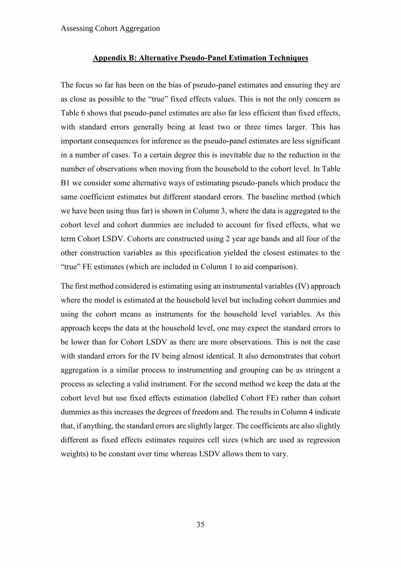
Assessing Cohort Aggregation
35
Appendix B: Alternative Pseudo-Panel Estimation Techniques
The focus so far has been on the bias of pseudo-panel estimates and ensuring they are
as close as possible to the “true” fixed effects values. This is not the only concern as
Table 6 shows that pseudo-panel estimates are also far less efficient than fixed effects,
with standard errors generally being at least two or three times larger. This has
important consequences for inference as the pseudo-panel estimates are less significant
in a number of cases. To a certain degree this is inevitable due to the reduction in the
number of observations when moving from the household to the cohort level. In Table
B1 we consider some alternative ways of estimating pseudo-panels which produce the
same coefficient estimates but different standard errors. The baseline method (which
we have been using thus far) is shown in Column 3, where the data is aggregated to the
cohort level and cohort dummies are included to account for fixed effects, what we
term Cohort LSDV. Cohorts are constructed using 2 year age bands and all four of the
other construction variables as this specification yielded the closest estimates to the
“true” FE estimates (which are included in Column 1 to aid comparison).
The first method considered is estimating using an instrumental variables (IV) approach
where the model is estimated at the household level but including cohort dummies and
using the cohort means as instruments for the household level variables. As this
approach keeps the data at the household level, one may expect the standard errors to
be lower than for Cohort LSDV as there are more observations. This is not the case
with standard errors for the IV being almost identical. It also demonstrates that cohort
aggregation is a similar process to instrumenting and grouping can be as stringent a
process as selecting a valid instrument. For the second method we keep the data at the
cohort level but use fixed effects estimation (labelled Cohort FE) rather than cohort
dummies as this increases the degrees of freedom and. The results in Column 4 indicate
that, if anything, the standard errors are slightly larger. The coefficients are also slightly
different as fixed effects estimates requires cell sizes (which are used as regression
weights) to be constant over time whereas LSDV allows them to vary.
Assessing Cohort Aggregation
36
Table B1: Alternative techniques for estimating Pseudo-panels
Aggregation
level Household
Cohort
Household with cohort
observations
FE IV
Cohort
LSDV
Cohort
FE
LSDV
Cohort Y
LSDV
House-hold Y
HHsize -0.092*** -0.093*** -0.093*** -0.094*** -0.093*** -0.093***
(0.004) (0.007) (0.007) (0.007) (0.003) (0.008)
ltot_asset 0.105*** 0.118*** 0.118*** 0.118*** 0.118*** 0.118***
(0.006) (0.012) (0.012) (0.013) (0.006) (0.014)
secondary 0.051*** 0.060* 0.060* 0.063** 0.060*** 0.060
(0.012) (0.032) (0.031) (0.032) (0.016) (0.037)
lnremit 0.019*** 0.025 0.025* 0.026* 0.025*** 0.025
(0.007) (0.016) (0.015) (0.016) (0.008) (0.019)
remittance -0.205** -0.298 -0.298* -0.308* -0.298*** -0.298
(0.080) (0.189) (0.181) (0.187) (0.092) (0.226)
Observations 8,645 8,790 1,727 1,727 8,790 8,790
R-squared 0.48 0.67 0.91 0.71 0.92 0.56
Note: The first two columns estimate using household level data to either estimate fixed effects
regression using the panel nature of the data or an IV regression using cohort means as instruments.
Columns 3 and 4 use cohort means to create a cohort level panel and account for cohort fixed effects
either using cohort dummies (Column 3) or fixed effects (Column 4). Cohort LSDV has been used in
the main analysis to estimate pseudo-panels. Columns 5 and 6 maintains the data at the household level
but the values of the explanatory variables are the cohort means. Column 5 uses the cohort means for the
dependent variable whereas Column 6 instead uses the household level values. Robust standard errors
in parentheses. *** p<0.01, ** p<0.05, * p<0.1
The final two methods are similar and involve estimating at the household level but
using the cohort mean observations rather than the household level observations. This
amounts to the cohort mean observations being repeated in the dataset the same number
of times as their cell sizes. Cohort dummies are included to account for fixed effects
and the regression is weighted by the negative of the square-root of the cell for
consistency with the weighting used in the cohort level regressions. The methods differ
in that ‘LSDV Cohort Y’ uses cohort mean values for the dependent variable as well
as the independent variables, whereas ‘LSDV Household Y’ does so only for the
independent variables and keeps the dependent variable values at the household level.
Both approaches have a certain advantage over using Cohort LSDV. Cohort Y produces
standard errors that are very similar to the FE errors, resulting in identical inference
with estimates having the same significance levels. Although estimating in such a
manner is questionable as it essentially involves artificially expanding the number of
observations by replication, it is the only method that produces errors similar to the FE
values. Thus it is best to continue using Cohort LSDV as the baseline, however one

Assessing Cohort Aggregation
37
could include Cohort Y alongside it in order to get inference closer to those at the
household level. The Household Y approach is not as useful for getting improved
standard errors, but has the advantage of producing an R-squared that is more consistent
with those from household level models. The R-squared is slightly larger than for the
FE model but far below those from other pseudo-panel models where the value often
exceeds 0.9. Thus if one is interested in a goodness-of-fit measure for pseudo-panel
models then the R-squared from a Household Y model may be the most suitable option.
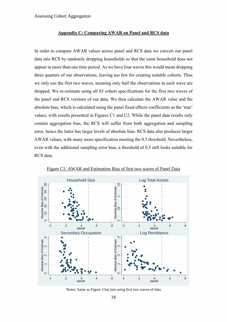
Assessing Cohort Aggregation
38
Appendix C: Comparing AWAR on Panel and RCS data
In order to compare AWAR values across panel and RCS data we convert our panel
data into RCS by randomly dropping households so that the same household does not
appear in more than one time period. As we have four waves this would mean dropping
three quarters of our observations, leaving too few for creating suitable cohorts. Thus
we only use the first two waves, meaning only half the observations in each wave are
dropped. We re-estimate using all 65 cohort specifications for the first two waves of
the panel and RCS versions of our data. We then calculate the AWAR value and the
absolute bias, which is calculated using the panel fixed effects coefficients as the ‘true’
values, with results presented in Figures C1 and C2. While the panel data results only
contain aggregation bias, the RCS will suffer from both aggregation and sampling
error, hence the latter has larger levels of absolute bias. RCS data also produces larger
AWAR values, with many more specification meeting the 0.5 threshold. Nevertheless,
even with the additional sampling error bias, a threshold of 0.5 still looks suitable for
RCS data.
Figure C1: AWAR and Estimation Bias of first two waves of Panel Data
Notes: Same as Figure 3 but just using first two waves of data
0.0
1.0
2.0
3.0
4.0
5A
bsolu
te B
ias o
f E
stim
ate
0 .2 .4 .6 .8AWAR
Household Size
0.0
5.1
.15
Absolu
te B
ias o
f E
stim
ate
0 .2 .4 .6 .8AWAR
Log Total Assets
0.1
.2.3
.4A
bsolu
te B
ias o
f E
stim
ate
0 .2 .4 .6 .8AWAR
Secondary Occupation
0.1
.2.3
.4A
bsolu
te B
ias o
f E
stim
ate
0 .2 .4 .6 .8AWAR
Log Remittance
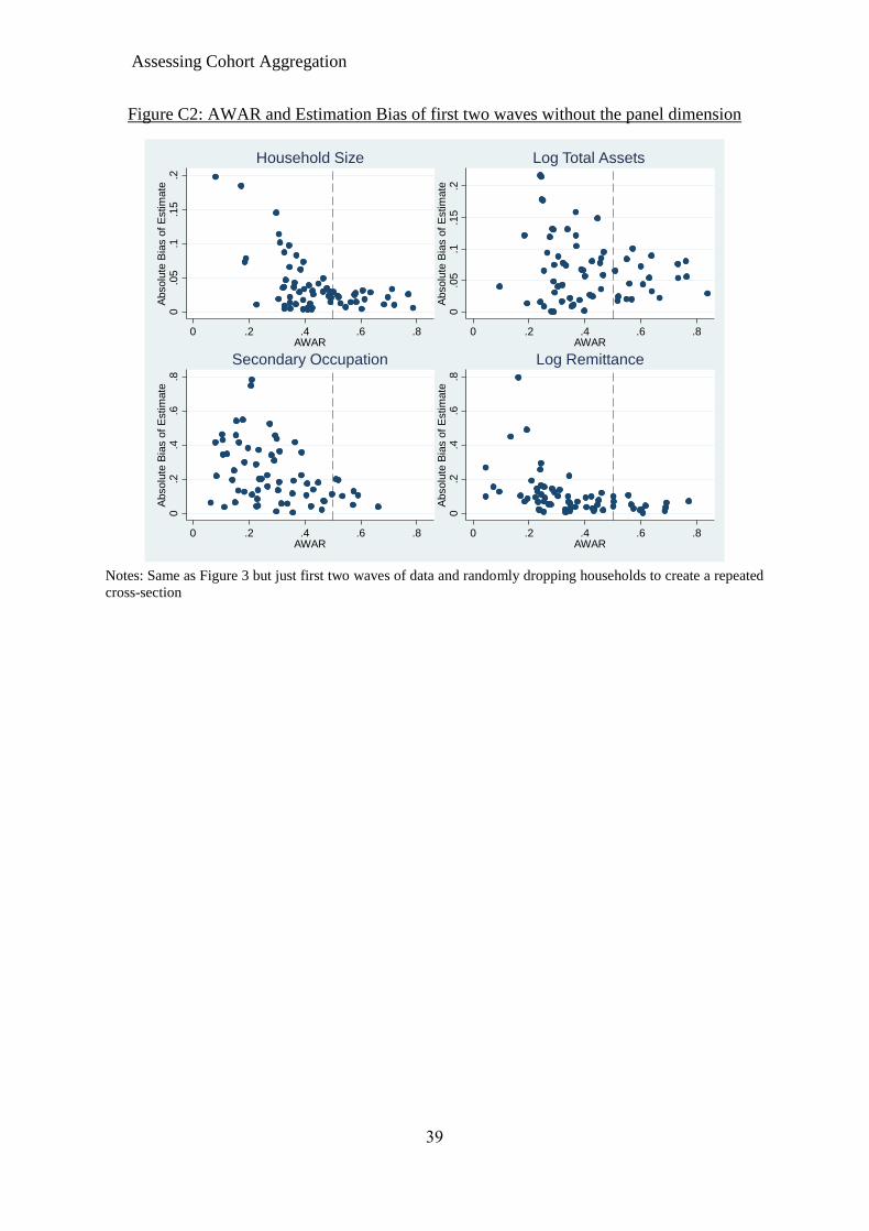
Assessing Cohort Aggregation
39
Figure C2: AWAR and Estimation Bias of first two waves without the panel dimension
Notes: Same as Figure 3 but just first two waves of data and randomly dropping households to create a repeated
cross-section
0.0
5.1
.15
.2A
bsolu
te B
ias o
f E
stim
ate
0 .2 .4 .6 .8AWAR
Household Size
0.0
5.1
.15
.2A
bsolu
te B
ias o
f E
stim
ate
0 .2 .4 .6 .8AWAR
Log Total Assets0
.2.4
.6.8
Absolu
te B
ias o
f E
stim
ate
0 .2 .4 .6 .8AWAR
Secondary Occupation
0.2
.4.6
.8A
bsolu
te B
ias o
f E
stim
ate
0 .2 .4 .6 .8AWAR
Log Remittance


![Index [assets.cambridge.org]assets.cambridge.org/97805218/60253/index/9780521860253_index… · aggregation. See bubble, aggregation; particle, aggregation; particle, concentration](https://img.pdfslide.us/doc/110x75/60634dbbe29a93467d378f87/index-aggregation-see-bubble-aggregation-particle-aggregation-particle.jpg)