Assessing Cognitive Achievement Growth During the Kindergarten and First Grade Years

July 2004 RR-04-22

ResearchReport

Donald A. Rock

Judy M. Pollack

Michael Weiss

Research & Development

Assessing Cognitive Achievement Growth During the Kindergarten and First Grade Years

Donald A. Rock, Judy M. Pollack, and Michael Weiss

ETS, Princeton, NJ

July 2004

ETS Research Reports provide preliminary and limiteddissemination of ETS research prior to publication. Toobtain a PDF or a print copy of a report, please visit:

www.ets.org/research/contact.html

Abstract

This study attempts to identify different patterns of cognitive growth in kindergarten and first

grade associated with selected subpopulations. The results are based upon a nationally

representative sample of fall kindergartners who were retested in the spring of their kindergarten

year and then again in the fall and spring of their first grade year. Of special interest here is the

estimation of the growth rates of subpopulations of children that are often considered to be at

risk, educationally and/or economically. This study also investigates whether or not the absence

of formal schooling during the summer differentially impacts subpopulations who are “at risk”

because they may lack a strong educational support system in the home.

Key words: Longitudinal, kindergarteners, cognitive, growth, multilevel, summer effect, at-risk

i

The research discussed here attempts to identify different patterns of growth in reading

and mathematics achievement associated with selected subpopulations in kindergarten and first

grade. Longitudinal data was collected at four time points: fall kindergarten, spring kindergarten,

fall first grade, and spring first grade. Of special interest here is the estimation of the growth

rates of subpopulations of children that are often considered to be at risk, educationally and/or

economically. In addition to estimating the amount of growth, this study will investigate how the

subpopulations may differ with respect to the quality of their growth. That is, we will also use a

criterion-referenced approach to measuring change that looks at how the subpopulations differ

with respect to where on the scale their growth is taking place. More specifically, this study

investigates how the growth patterns in reading and mathematics may differ by: (a) the highest

educational level achieved by a parent, (b) gender of the child, (c) ethnicity, and (d) school

sector.

This study will also investigate the summer effect and whether or not the relative absence

of formal schooling during the summer may have a differential negative impact on the cognitive

growth of particular subpopulations who are at risk because they lack a strong educational

support system in the home. The literature on summer learning is rather extensive. However,

most if not all of the literature deals with the absence or presence of the summer effect from

grades 1 on up. This study will be able to fill in the gap with respect to potential differential

summer learning decline using the spring kindergarten to fall first grade year time points. Heyns

(1998) found that pupils in Atlanta schools gained more during the school year than during the

summer, and that summer learning was inversely related to parents’ educational level. Entwisle,

Alexander, and Olson (1997) found that school year learning was unrelated to socioeconomic

status while summer learning was negatively related to socioeconomic status in both reading and

mathematics. Entwisle and Alexander (1992, 1994) also investigated the relationship of ethnicity

with summer learning compared with in-school learning. Cooper, Nye, Charlton, Lindsey, and

Greathouse (1996) conducted a meta-analysis of summer learning studies and concluded that

achievement test scores decline when schools are not in session. Many of the earlier studies did

not use vertically equated tests with a common scale spanning grades of interest, which

theoretically would be more sensitive to change as well as minimize both floor and ceiling

effects. To our knowledge, no other study used a vertically equated adaptive test. It is possible

that the finding of a summer loss as opposed to a de-acceleration in growth may be due to a lack

1

of sensitivity to growth and/or floor and ceiling effects that may characterize the repetition of the

same or a parallel form on successive testings. The potential floor and ceiling effects of

nonadaptive measurement instruments could seriously distort gain comparisons between

disadvantaged and advantaged children, who tend to occupy the opposite tails of ability

distributions.

The data for this study comes from the Early Childhood Longitudinal Study,

Kindergarten Class of 1998-99 (ECLS-K) sponsored by the U. S. Department of Education,

National Center for Education Statistics. The ECLS-K base year sample was a national

probability sample of approximately 20,000 children who entered kindergarten in fall 1998. The

ECLS-K longitudinal study is designed to follow children’s progress in a number of cognitive

areas from kindergarten entry to the spring of fifth grade. The study described here focuses on

changes in early reading and mathematics skills taking place during the first 2 years of schooling.

This study used mathematics and reading scores gathered at four points in time: fall

kindergarten, spring kindergarten, fall first grade, and spring first grade. The reading and

mathematics scale scores gathered at the four time points were based on individually

administered adaptive tests.

Sample

The analysis sample was restricted to those children who had both reading and

mathematics scores in the fall (Time Point 1) and spring (Time Point 2) of their kindergarten

year and remained in the same school during their kindergarten and first grade years. They also

had to have complete information on: (a) gender, (b) parental education, (c) ethnicity, and (d)

school sector. This reduced sample numbered 14,707 children. At Time Point 3 (fall first grade)

a probability subsample of the base year sample numbering about 5,000 was retested, of whom

3,032 children met the requirements described above. Estimates of summer gains were based on

this subsample, targeting the growth occurring between spring kindergarten (Time Point 2) and

fall first grade (Time Point 3). The assessment at the fourth time point (spring first grade)

included 10,406 children who matched the children meeting the requirements for inclusion in the

longitudinal sample being analyzed here.

2

Method

Multilevel modeling (Bryk & Raudenbush, 1992; Goldstein, 1995; Snijders & Bosker,

1999) was used to investigate variation in growth curves at both the school and child levels.

Multilevel software programs are particularly appropriate when the data have a hierarchical

organization where units at one level are nested within units at one or more higher levels. The

data organization for longitudinal studies is inherently hierarchical with occasions nested under

individuals. In addition, the ECLS-K sampling design was a two-stage design that sampled

schools and then children within schools, leading to a more complex three-level hierarchy. The

ability of multilevel software to automatically correct the standard errors for the clustering

effects associated with having children from the same school, along with the ability to handle

missing data at the different time points, makes the methodology particularly attractive for large

scale longitudinal studies. Rival procedures such as the multivariate analysis of covariance

(MANCOVA), which can relax assumptions about the error structure, are not typically able to

efficiently handle missing data on the repeated occasions or to compensate for the clustering

effects. Therefore the multilevel approach was applied here using MlwiN software (Goldstein et

al., 1998) with the school sample being Level 3 in the model; the child sample, Level 2, and the

four testing occasions within the child sample, Level 1. Panel sampling weights were used in all

analyses. The panel sample weights are longitudinal weights that apply to children who

participated in the data collection at all time points (excluding the fall first grade subsample) and

weight up to the population of kindergarteners in fall 1998. Children who joined the ECLS-K

sample after the base year (fall kindergarten) would have a panel weight of 0 regardless of

whether they were assessed or not.

The dependent measures for each of the four occasions for each child were scale scores in

reading and mathematics. These scale scores were obtained from longitudinally equated adaptive

tests in each subject. On each testing occasion, a child received first stage routing tests in reading

and mathematics, which were designed to assess the child's approximate ability level. Depending

on the routing test score, each child was then administered one of three second-stage tests in each

subject. Children who achieved high scores on the routing test received a difficult second stage

form, while those with low scores received the easiest second stage form. Children in the middle

range on the routing test received the middle difficulty second stage form. The resulting targeting

of item difficulties to the child’s ability level maximized measurement precision while

3

minimizing the potential for floor and ceiling effects. Item response theory (IRT) scaling (Lord,

1980) was carried out, using items shared across forms to arrive at a common vertically equated

scale.

The scale scores are just one of the family of IRT-based measures available on the ECLS

public use data file (National Center for Education Statistics, 2002). The scale scores are

particularly appropriate as overall outcome measures for multilevel analysis because of their

continuous nature and relatively normal distribution. The theoretical range of the reading scale

scores is 0 to 92, while the comparable range for the mathematics scale scores is 0 to 64. The

reading scale score is an IRT-based estimate of the number of items a child would have answered

correctly if the whole pool of 92 items that appeared in all forms of the tests had been

administered. Similarly, the mathematics scale scores are estimates of number-correct scores

based on the pool of 64 unique mathematics items. The actual reading scores ranged from a low

of 10.5 to 89.0, while the comparable range in mathematics was 7.0 to 60.5. The reading scale

was defined to have five criterion-referenced points, marking an ascending order of reading and

prereading skills. The lower end of the hierarchical set of skills dealt with letter recognition and

then moved up through beginning sounds, ending sounds, simple sight words, and finally

comprehension of words in context at the upper end of the scale. The set of mathematics scores

also included criterion-referenced markers, but these are not addressed in this paper.

In order to explain the variation in intercepts and slopes at both the child and school

levels, age, school sector, individual demographic variables, and their interactions with age at

time of testing were added to the multilevel models. The regression weights associated with

subgroup variables (e.g., ethnicity, gender) provided estimates of the difference in subgroup

intercepts as well as significance tests. The regression weights associated with the interaction

terms provide estimates of the different rates of growth and their significance tests for the

subgroups.

In the multilevel analysis, a sequence of models of increasing complexity were fit to the

data beginning with a simple regression of reading (or mathematics) scores on four occasions

based on the child’s age at time of testing, measured in months. In this simple model (Model 0),

only the intercept was considered random at both Level 3 (school) and Level 2 (child). This

linear growth curve model allows both schools and children to have different intercepts for their

regression lines. In this and all succeeding models, age is a time-covarying explanatory variable,

4

which is key to defining and interpreting the growth curves at both the school and child levels.

Age at time of testing is very important because the time lapse between testings varies among

occasions and to a certain extent across children within the same occasion. Since age is a carrier

for both maturation and accumulated formal and informal learning, age is a critical

control/explanatory variable. The equation for Model 0 is as follows:

0 1 1

0 0 0 0

ijk ijk ijk

ijk k jk ijk

y x

v u e0

β β

β β= = +

= + + + (1)

Where the reading (or math) score for the iijky = th test administration for the jth child in

the kth school, and

1ijkx = age of the child at the ith testing occasion measured as deviations in months from

the overall mean age at the time of the initial assessment (Time 1), and

1β = regression of reading (or math) on age at time of testing, assumed in this model to

be fixed, meaning that the regression slopes are constant across children and schools, and

0β = overall average intercept, which is assumed to be a random effect in this base

model, and thus we also have

0kv = estimate of the deviation of the kth school’s intercept from the average intercept,

and

0 jku = estimate of the deviation of the jth child’s intercept from the average within school

intercept, and

0ijke = residual variation in reading (or math) scores unexplained by the model.

5

The next, more complex model (Model 1) is the same as the above model with the

exception that the slopes are also assumed to be a random effect, and thus we estimate variation

due to schools and children having different slopes associated with their growth curves. That is,

the next model, Model 1, allows the slopes of reading scores on ages as well as their intercepts to

vary by school and child. Model 2 simply adds age squared as a fixed effect to Model 1 in order

to investigate whether the growth curves have a significant nonlinear component. Model 3

introduces the dummy-coded main effects of the explanatory variables (gender, parental

education, school sector, and ethnicity) as fixed effects. The addition of the fixed main effects

would be expected to explain some of the variation in the intercepts at both the school and child

level. In addition, the regression weights associated with the main effects reflect differences

among subgroups in their reading and mathematics scores at entry to kindergarten. Model 4 adds

the interactions of the explanatory variables with age to the main effects from Model 3. The

introduction of the interactions is primarily an attempt to explain the variability in the slopes of

the growth curves at both the school and individual level. The regression weights in the fixed

part of model associated with specific age by explanatory variable interactions will address the

question of how growth rates differ for populations considered to be at risk, compared with those

considered to be advantaged.

After completing the multilevel analysis, a series of regressions were run in an attempt to

pinpoint the presence or absence of a differential impact associated with summer learning.

While gains in scale scores tell us how much the child has gained, they do not tell us

where on the scale the gains are being made. Two children may have each gained 6 score points

on the overall reading scale, but one child is gaining in his/her proficiency in ending sounds

(located in the middle of the scale) while the other child is gaining in beginning reading for

comprehension (the upper end of the scale). In this example, the quantitative gains in terms of

scale score points are equivalent, but there is a qualitative difference that is at least as important

in understanding children's gain scores. The adaptive tests used here were designed to be both

norm-referenced and criterion-referenced. The criterion-referenced scale points were designed to

mark milestones in the development of early reading skills. In this study, one particular criterion-

referenced milestone was used to aid in the interpretation of the overall gains. That is, in addition

to knowing how much a child has gained, we would like to know if he/she is gaining on that part

of the scale where one of the critical reading behavior milestones is located. For the purposes of

6

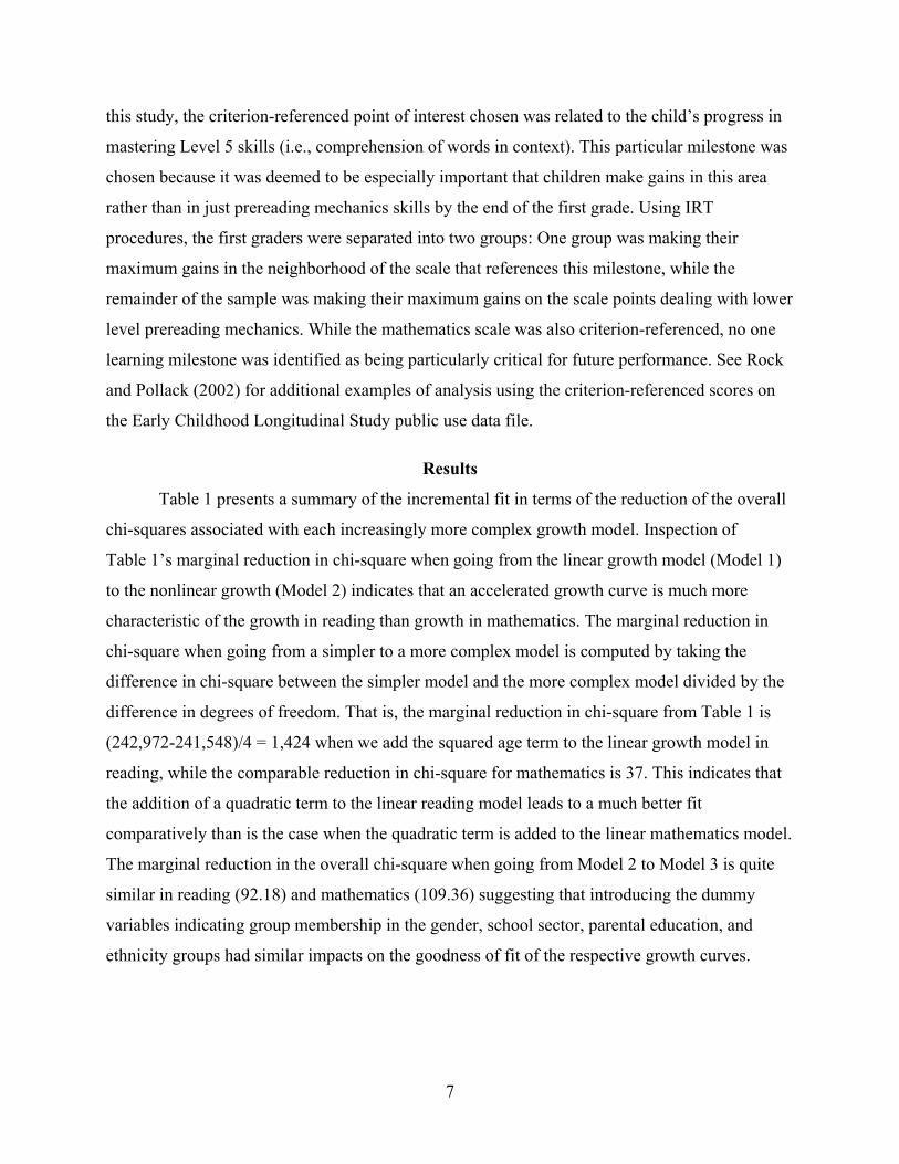
this study, the criterion-referenced point of interest chosen was related to the child’s progress in

mastering Level 5 skills (i.e., comprehension of words in context). This particular milestone was

chosen because it was deemed to be especially important that children make gains in this area

rather than in just prereading mechanics skills by the end of the first grade. Using IRT

procedures, the first graders were separated into two groups: One group was making their

maximum gains in the neighborhood of the scale that references this milestone, while the

remainder of the sample was making their maximum gains on the scale points dealing with lower

level prereading mechanics. While the mathematics scale was also criterion-referenced, no one

learning milestone was identified as being particularly critical for future performance. See Rock

and Pollack (2002) for additional examples of analysis using the criterion-referenced scores on

the Early Childhood Longitudinal Study public use data file.

Results

Table 1 presents a summary of the incremental fit in terms of the reduction of the overall

chi-squares associated with each increasingly more complex growth model. Inspection of

Table 1’s marginal reduction in chi-square when going from the linear growth model (Model 1)

to the nonlinear growth (Model 2) indicates that an accelerated growth curve is much more

characteristic of the growth in reading than growth in mathematics. The marginal reduction in

chi-square when going from a simpler to a more complex model is computed by taking the

difference in chi-square between the simpler model and the more complex model divided by the

difference in degrees of freedom. That is, the marginal reduction in chi-square from Table 1 is

(242,972-241,548)/4 = 1,424 when we add the squared age term to the linear growth model in

reading, while the comparable reduction in chi-square for mathematics is 37. This indicates that

the addition of a quadratic term to the linear reading model leads to a much better fit

comparatively than is the case when the quadratic term is added to the linear mathematics model.

The marginal reduction in the overall chi-square when going from Model 2 to Model 3 is quite

similar in reading (92.18) and mathematics (109.36) suggesting that introducing the dummy

variables indicating group membership in the gender, school sector, parental education, and

ethnicity groups had similar impacts on the goodness of fit of the respective growth curves.

7

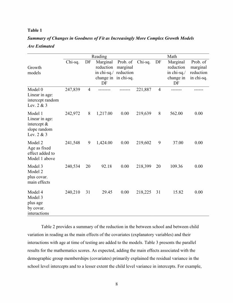
Table 1

Summary of Changes in Goodness of Fit as Increasingly More Complex Growth Models

Are Estimated

Reading Math

Growth models

Chi-sq. DF Marginalreductionin chi-sq./ change in

DF

Prob. of marginal reductionin chi-sq.

Chi-sq. DF Marginal reduction in chi-sq./ change in

DF

Prob. of marginal reduction in chi-sq.

Model 0 Linear in age: intercept random Lev. 2 & 3

247,839 4 -------- ------- 221,887 4 ------- ------

Model 1 Linear in age: intercept & slope random Lev. 2 & 3

242,972 8 1,217.00 0.00 219,639 8 562.00 0.00

Model 2 Age as fixed effect added to Model 1 above

241,548 9 1,424.00 0.00 219,602 9 37.00 0.00

Model 3 Model 2 plus covar. main effects

240,534 20 92.18 0.00 218,399 20 109.36 0.00

Model 4 Model 3 plus age by covar. interactions

240,210 31 29.45 0.00 218,225 31 15.82 0.00

Table 2 provides a summary of the reduction in the between school and between child

variation in reading as the main effects of the covariates (explanatory variables) and their

interactions with age at time of testing are added to the models. Table 3 presents the parallel

results for the mathematics scores. As expected, adding the main effects associated with the

demographic group memberships (covariates) primarily explained the residual variance in the

school level intercepts and to a lesser extent the child level variance in intercepts. For example,

8

using the variance estimates from Table 2 suggests that adding the subgroup main effects to

Reading Model 2 led to a 51% marginal reduction (17.277-8.406)/17.277 in the school level

variation in intercepts. Similarly, the addition of the main effects to Model 2 led to a 9%

marginal reduction (68.629-62.329)/68.629 in the student level variation in intercepts.

Table 2

Reduction in the Variance of Intercepts and Slopes in Reading Scores at the School and Child

Level as the Explanatory Variables (Covariates) and Their Interactions Are Introduced

Variance of intercepts with standard errors ( )

Variance of slopes with standard errors( ) Growth model

School Child School Child

Model 2 Linear and quadratic in age at testing; intercepts and linear slopes random

17.277

(1.230)

68.629

(1.229)

0.043

(0.003)

0.176

(0.005)

Model 3 Model 2 above plus main effects of covariates

8.406

(0.744)

62.329

(1.124)

0.043

(0.003)

0.176

(0.005)

Model 4 Model 3 above plus age at testing by covarariate interaction

8.274

(0.735)

61.791

(1.124)

0.033

(0.003)

0.169

(0.005)

The comparable numbers from Table 3 in mathematics were 66% reduction in school

level intercepts and 8% in the child level intercept variance. As expected, adding the interactions

had very little effect on the intercepts. However, the addition of the interaction terms to the main

effects model in reading led to a 23% marginal reduction in the residual variation in slopes at the

school level. In terms of residual variation in the reading slopes at the child level, the marginal

reduction was 4%. In mathematics, the comparable numbers were 23% at the school level and 0

% at the child level. Undoubtedly part of the better prediction of both intercepts and slopes at the

school level than at the child level from the background explanatory variables is due to the fact

that both slopes and intercepts are more reliable at the school level.

9

Table 3

Reduction in the Variance of Intercepts and Slopes in Mathematics Scores at the School and

Child Level as the Explanatory Variables (Covariates) and Their Interactions Are Introduced

Variance of intercepts with standard errors ( )

Variance of slopes with standard errors( ) Growth model

School Child School Child Model 2 Linear and quadratic in age at testing; intercepts and linear slopes random

10.884

(0.768)

42.090

(0.746)

0.013

(0.001)

0.041

(0.002)

Model 3 Model 2 above plus main effects of covariates

3.673

(0.379)

38.596

(0.695)

0.013

(0.001)

0.041

(0.002)

Model 4 Model 3 above plus age at testing by covarariate interaction

3.703

(0.380)

38.614

(0.695)

0.010

(0.001)

0.041

(0.002)

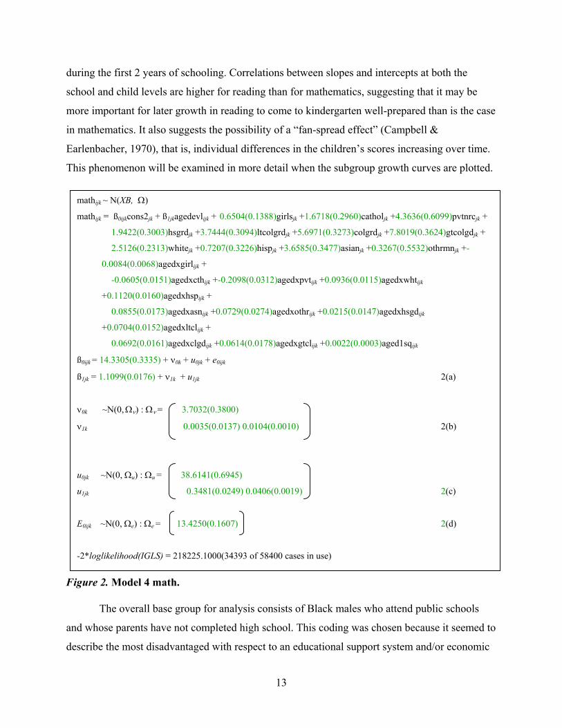
Figure 1 presents the regression weights and their standard errors (in parenthesis) for the

fixed part of Model 4 as well as the variances and covariances of the random intercepts and

slopes for the full model (Model 4) in reading. Figure 2 presents the comparable model for the

mathematics scores. All explanatory variables in the model with the exception of age at time of

testing are considered categorical and are dummy- coded. For example, girls are coded 1 and

boys are coded 0. The contrast group (i.e., the 0-coded group) for the gender comparison does

not appear in the equation. The regression weight associated with girls in the reading model is

2.3139, indicating that when controlling for all other variables in the model, girls start school, on

average, at 2.3139 scale points higher than boys. Similarly, based on the regression weight in the

reading model, children who are enrolled in Catholic schools start kindergarten at 1.3183 reading

scale points higher than the 0-coded contrast group, children attending public schools. This

interpretation of the main effects regression weights is possible because of the way the age

variable is scaled. The age variable is measured as deviations from the mean age at Time Point 1

(kindergarten entry). The interaction terms of age with the dummies for the main effect variables

have a similar interpretation. For example, the regression weight for the age by gender

10

interaction, agedxgirl equals .0957, indicating that the regression slope of reading on age at time

of testing for girls is .0957 scale points steeper than that for boys. This increment in slope for

girls over that of the boys is statistically significant as shown by the regression weight divided by

its standard error (.0957/.0109) giving a t-statistic of 8.78.

readijk ~ N(XB, Ω)

readijk = ß0ijkcons2jk + ß1jkagedevlijk + 2.3139(0.1770)girlsjk +1.3183(0.4120)catholjk +7.7901(0.8317)pvtnrcjk +

2.5648(0.3838)hsgrdjk +4.4044(0.3960)ltcolgrdjk +6.5493(0.4194)colgrdjk +9.6554(0.4651)gtcolgdjk +

1.0662(0.3029)whitejk +-0.1723(0.4195)hispjk +4.2063(0.4524)asianjk +-0.0200(0.7227)othrmnjk +

0.0957(0.0109)agedxgirlijk +-0.0140(0.0258)agedxcthijk +-0.1490(0.0524)agedxpvtijk

+0.1197(0.0188)agedxwhtijk +

0.1306(0.0261)agedxhispijk +0.2337(0.0282)agedxasnijk +0.0590(0.0447)agedxothrijk

+0.1358(0.0236)agedxhsgdijk +

0.2331(0.0244)agedxltclijk +0.2629(0.0259)agedxclgdijk +0.2622(0.0287)agedxgtclijk

+0.0187(0.0004)agedlsqijk

ß0ijk = 16.884(0.4344) + ν0k + u0jk + e0ijk

ß1jk = 1.0825(0.0281) + ν1k + u1jk 1(a)

ν0k ~N(0, Ων) : Ων = 8.2738(0.7350)

ν1k 0.1251(0.0331) 0.0333(0.0029) 1(b)

u0jk ~N(0, Ωu) : Ωu = 61.7917(1.1242)

u1jk 1.3,786(0.0498) 0.1693(0.0045) 1(c)

E0ijk ~N(0, Ωe) : Ωe = 22.4472(0.2693) 1(d)

-2*loglikelihood(IGLS) = 240210.2000(34390 of 58400 cases in use)

Figure 1. Model 4 reading.

While most of the naming of the explanatory variables in Figures 1 and 2 are self-

explanatory, additional information is helpful for some. The critical time covarying growth

variable, agedev1, refers to age in months at time of testing measured as deviations from the

Time Point 1 mean. The variables Cathol and pvtnrc refer to whether a child attends a Catholic

11

or a private non-Catholic school. The missing variable public, identifying children attending a

public school, is the contrast group. The variables hsgrd, ltcolgrd, colgrd, and gtcolgd refer to the

highest educational level achieved by one or both parents and stands for high school graduate,

some college, college graduate, and graduate work beyond a bachelor’s degree, respectively. The

missing parental group, less than high school graduate, is the contrast or base group for this set

of dummy variables. The group of dummy variables reflecting ethnicity, white, hisp, asian, and

othmn, refers to White, Hispanic, Asian, and other minority children not including Black,

respectively. The missing group, Black children, was the contrast group. The variable aged1sq

indicates the age in months at time of testing squared. The cross-product terms refer, of course,

to the interactions of age at time of testing with each of the respective main effects. For example,

agedxgirl refers to the interaction of the dummy-variable girls with time of testing. If the

regression weight associated with this term is positive and significant, one would conclude that

girls have a steeper linear slope to their growth curve than do boys.

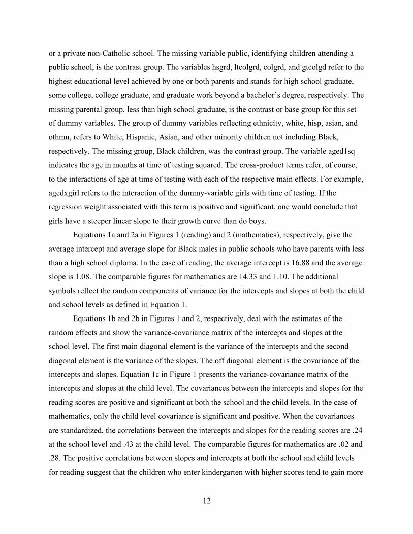
Equations 1a and 2a in Figures 1 (reading) and 2 (mathematics), respectively, give the

average intercept and average slope for Black males in public schools who have parents with less

than a high school diploma. In the case of reading, the average intercept is 16.88 and the average

slope is 1.08. The comparable figures for mathematics are 14.33 and 1.10. The additional

symbols reflect the random components of variance for the intercepts and slopes at both the child

and school levels as defined in Equation 1.

Equations 1b and 2b in Figures 1 and 2, respectively, deal with the estimates of the

random effects and show the variance-covariance matrix of the intercepts and slopes at the

school level. The first main diagonal element is the variance of the intercepts and the second

diagonal element is the variance of the slopes. The off diagonal element is the covariance of the

intercepts and slopes. Equation 1c in Figure 1 presents the variance-covariance matrix of the

intercepts and slopes at the child level. The covariances between the intercepts and slopes for the

reading scores are positive and significant at both the school and the child levels. In the case of

mathematics, only the child level covariance is significant and positive. When the covariances

are standardized, the correlations between the intercepts and slopes for the reading scores are .24

at the school level and .43 at the child level. The comparable figures for mathematics are .02 and

.28. The positive correlations between slopes and intercepts at both the school and child levels

for reading suggest that the children who enter kindergarten with higher scores tend to gain more

12

during the first 2 years of schooling. Correlations between slopes and intercepts at both the

school and child levels are higher for reading than for mathematics, suggesting that it may be

more important for later growth in reading to come to kindergarten well-prepared than is the case

in mathematics. It also suggests the possibility of a “fan-spread effect” (Campbell &

Earlenbacher, 1970), that is, individual differences in the children’s scores increasing over time.

This phenomenon will be examined in more detail when the subgroup growth curves are plotted.

mathijk ~ N(XB, Ω)

mathijk = ß0ijkcons2jk + ß1jkagedevlijk + 0.6504(0.1388)girlsjk +1.6718(0.2960)catholjk +4.3636(0.6099)pvtnrcjk +

1.9422(0.3003)hsgrdjk +3.7444(0.3094)ltcolgrdjk +5.6971(0.3273)colgrdjk +7.8019(0.3624)gtcolgdjk +

2.5126(0.2313)whitejk +0.7207(0.3226)hispjk +3.6585(0.3477)asianjk +0.3267(0.5532)othrmnjk +-

0.0084(0.0068)agedxgirlijk +

-0.0605(0.0151)agedxcthijk +-0.2098(0.0312)agedxpvtijk +0.0936(0.0115)agedxwhtijk

+0.1120(0.0160)agedxhspijk +

0.0855(0.0173)agedxasnijk +0.0729(0.0274)agedxothrijk +0.0215(0.0147)agedxhsgdijk

+0.0704(0.0152)agedxltclijk +

0.0692(0.0161)agedxclgdijk +0.0614(0.0178)agedxgtclijk +0.0022(0.0003)aged1sqijk

ß0ijk = 14.3305(0.3335) + ν0k + u0jk + e0ijk

ß1jk = 1.1099(0.0176) + ν1k + u1jk 2(a)

ν0k ~N(0, Ων) : Ων = 3.7032(0.3800)

ν1k 0.0035(0.0137) 0.0104(0.0010) 2(b)

u0jk ~N(0, Ωu) : Ωu = 38.6141(0.6945)

u1jk 0.3481(0.0249) 0.0406(0.0019) 2(c)

E0ijk ~N(0, Ωe) : Ωe = 13.4250(0.1607) 2(d)

-2*loglikelihood(IGLS) = 218225.1000(34393 of 58400 cases in use)

Figure 2. Model 4 math.

The overall base group for analysis consists of Black males who attend public schools

and whose parents have not completed high school. This coding was chosen because it seemed to

describe the most disadvantaged with respect to an educational support system and/or economic

13

well-being. As a result, most of the regression weights are positive. Regression weights

associated with the main effects (e.g., White, Hispanic, girls) in Figures 1 and 2 give the

difference in scale score points between each group’s intercept and the contrast group intercept.

For example, controlling for all the other demographics, the White children started 1.0662 points

ahead of the Black children. That is, their intercepts differed by 1.0662 points. The regression

weights associated with an interaction term such as agedxhisp give the difference between the

slope of the Hispanic children and the slope of the contrast group, Black children. In reading, this

coding led to all but two main effects having statistically significant positive contrasts based on

the ratio of their regression coefficients to their standard errors. This indicated that the base

group started significantly below all other groups with the exception of the Hispanic group

(b = -.1723; t = -.41, p = .42) and the other minority group (b = -.0200; t = .03, p = .49), which

were not significantly different from the Black base contrast group at kindergarten entry. The

t-statistic is, of course, simply the regression weight shown in Figure 1 divided by its standard

error, shown in parentheses also in Figure 1.

The Hispanic children, however, had a significantly greater linear growth rate in reading,

as indicated by the regression weight associated with their interaction term (b = .1306; t = 5.0,

p = .00), suggesting that, on average, they are growing at a rate of .13 of a reading scale point

more per month than are the Black children.

In mathematics, the regression weight associated with the Hispanic children (b = .7207;

t = 2.23, p = .00) indicates that they started out significantly higher than the Black children and

also showed a significantly greater linear growth rate as reflected in the coefficient for their

interaction term (b = .1120; t = 7.0, p = .00).

What is particularly impressive is the advantage that children have who come from

homes where the highest parent education is a high school degree or higher. Such children begin

kindergarten 2.56 to 9.65 points higher on the reading scale than children from the base parental

education group (less than a high school education). At the higher end of the parental education

scale, college degree or higher, the children start with a 6.54 to 9.65 advantage as indicated by

the regression weights associated with a parental college degree (b = 6.54; t = 15.61, p = .00) and

that associated with graduate work beyond college (b = 9.65; t = 20.76, p = .00). Not only do

they enter the formal education system with a formidable head start, but they also continue to

grow at a faster rate after entering the school system, as evidenced by their significantly higher

14

linear slopes. More specifically, other things being equal, the children whose parents have a

college degree are gaining .26 reading scale points more per month than are children whose

parents have not finished high school. Similar but less pronounced effects are found in

mathematics where the higher education levels of the parents are related to increments in growth

rates of .06–07 points per month.

It is interesting to note that while children who attended Catholic and private non-

Catholic schools started with significantly higher average scores than those of public school

children, the rate of gain in reading for the Catholic school children was not significantly

different from that of the public school children. The private non-Catholic school children's rate

of gain was significantly less than that of the public school children over the first two years of

schooling in both reading and mathematics. It would seem that in these early stages of

development the public school children appear to be closing some of the original gap found

between their performance in reading at kindergarten entry and that of the private non-Catholic

school children.

A summary of the results shown in Figures 1 and 2 suggest that:

• Girls start kindergarten with significantly better reading or prereading skills than boys

(b = 2.3139; t = 13.07; p = .00) and girls are growing their reading skills at a significantly

greater rate than are boys (b = .0957; t = 8.78; p = .00). That is, the regression weight

associated with girls (b = 2.314) in Figure 1 divided by its standard error (.177) gives the

t-statistic of 13.07 for intercept differences for girls and boys. Similarly, the significance

of the difference in growth rates for girls and boys is given by the regression weight

associated with the interaction of the dummy variable girls with age at time of testing

(b = .0957) divided by its standard error (.0109), also from Figure 1, resulting in the t-

statistic of 8.78.

• Girls start kindergarten performing significantly better than boys in mathematics

(t = 4.71; p = .00) but show no significant differences in growth rate (t = -1.24; p = .22).

• Other things being equal, the public school children enter kindergarten significantly

behind in reading compared to their counterparts in private and Catholic schools

(t = 9.37;p = .00: t = 3.12; p = .00, respectively). However, other things being equal, the

public school children are growing significantly faster in reading over the first two years

15

of schooling than are the private school children (t = 2.84; p = .01). Growth rates in

reading show no significant differences between public and Catholic school children.

• Mathematics results are similar to reading: Public school children start kindergarten with

deficits in mathematics (t = 7.15; p = .00: t = 5.65; p = .00) compared to private and

Catholic school children, respectively.

• However, Catholic and private non-Catholic school children grew at a lesser rate than did

the public school children in mathematics (t = 4.01; p = .00: t = 6.72; p = .00 for the

Catholic and private non-Catholic schools, respectively).

• In terms of ethnicity, White and Asian children began kindergarten significantly ahead of

Black children in reading (t = 3.53; p = .00: t = 9.33; p = .00, respectively). There were no

significant differences between Black children and Hispanic children or Black children

and other minority children in reading skills at entry to kindergarten. White, Asian, and

Hispanic children all grew at a significantly greater rate than did the Black children

(t = 6.36; p = .00: t = 8.28, p = .00: t = 5.00; p = .00, respectively). There was no

difference in the rate of gain in reading between the other minority and Black children.

• In mathematics, all ethnic groups with the exception of other minority started

kindergarten significantly ahead of the Black children (t’s ranged from 2.23; p = .02 to

t = 10.90; p = .00). With respect to growth rates in mathematics, all subgroups, White,

Asian, Hispanic, and other minority, grew at a faster rate than did the Black children (t’s

ranged from a low of 2.66; p = .01 for other minority children to a high of t = 8.14; p = .00

for the White children). It is interesting to note that Asian children started kindergarten

with greater skills in both reading and mathematics than any other ethnic group. They also

had the highest growth rate in reading of any ethnic group.

• In terms of parents’ education, children from all parental groups possessing a high school

degree or more advanced educations started kindergarten significantly ahead in reading

compared with children of parents with less than a high school degree. The t’s ranged

from a low of 6.47; p = .00 for children who had at least one parent with a high school

degree to 21.67; p = .00 for those children who had at least one parent with education

beyond a college degree. Growth rates were significantly greater in reading for all other

16

parental education groups when contrasted with children of parents with less than a high

school degree. The t’s ran from a low of 5.75; p = .00 for children of parents with a high

school degree to a high of 10.15; p = .00 for the children having a college educated parent.

• Mathematics scores for the same parent education contrasts showed similar patterns of

advantage at entry to kindergarten. The t’s ranged from a low of t = 6.46; p = .00 for

children of high school graduates to a high of t = 21.52; p = .00 for those children who

had one or more parents who did graduate work beyond college. Similar to the case in

reading, growth rates in mathematics performance increased with increases in parental

education with one exception: the contrast between children of parents with a high school

degree and those without a high school degree was not significant (t = 1.46; p = .14).

Summer Learning Effect

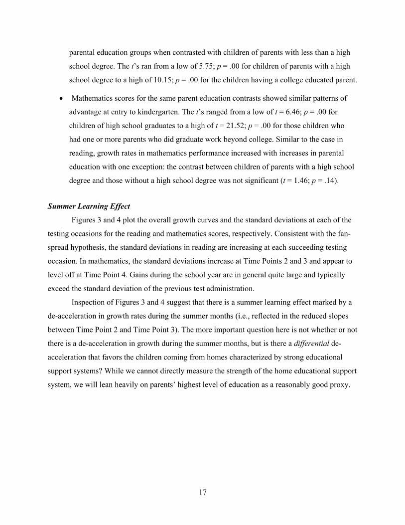
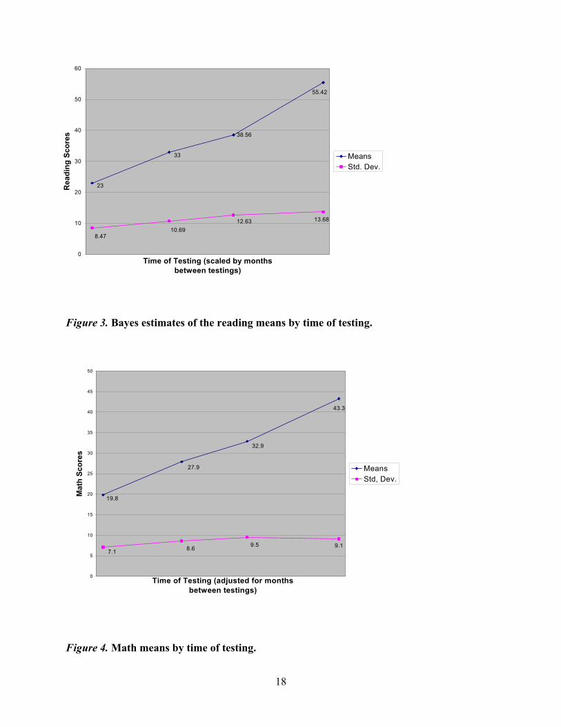
Figures 3 and 4 plot the overall growth curves and the standard deviations at each of the

testing occasions for the reading and mathematics scores, respectively. Consistent with the fan-

spread hypothesis, the standard deviations in reading are increasing at each succeeding testing

occasion. In mathematics, the standard deviations increase at Time Points 2 and 3 and appear to

level off at Time Point 4. Gains during the school year are in general quite large and typically

exceed the standard deviation of the previous test administration.

Inspection of Figures 3 and 4 suggest that there is a summer learning effect marked by a

de-acceleration in growth rates during the summer months (i.e., reflected in the reduced slopes

between Time Point 2 and Time Point 3). The more important question here is not whether or not

there is a de-acceleration in growth during the summer months, but is there a differential de-

acceleration that favors the children coming from homes characterized by strong educational

support systems? While we cannot directly measure the strength of the home educational support

system, we will lean heavily on parents’ highest level of education as a reasonably good proxy.

17

38.56

23

33

55.42

12.63

8.4710.69

13.68

0

10

20

30

40

50

60

Time of Testing (scaled by months between testings)

Rea

ding

Sco

res

MeansStd. Dev.

Figure 3. Bayes estimates of the reading means by time of testing.

32.9

19.8

27.9

43.3

9.19.57.1 8.6

0

5

10

15

20

25

30

35

40

45

50

Time of Testing (adjusted for months between testings)

Mat

h Sc

ores

MeansStd, Dev.

Figure 4. Math means by time of testing.

18

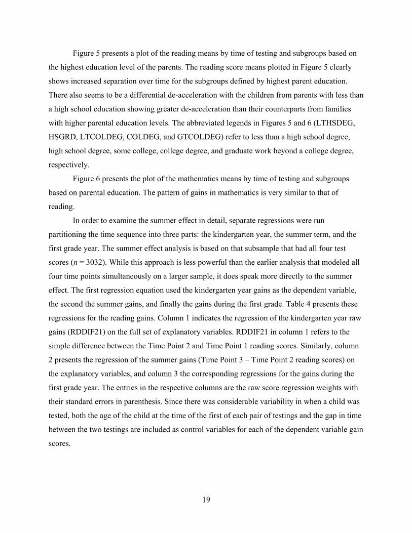
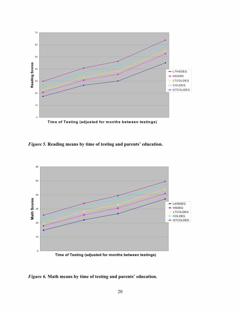
Figure 5 presents a plot of the reading means by time of testing and subgroups based on

the highest education level of the parents. The reading score means plotted in Figure 5 clearly

shows increased separation over time for the subgroups defined by highest parent education.

There also seems to be a differential de-acceleration with the children from parents with less than

a high school education showing greater de-acceleration than their counterparts from families

with higher parental education levels. The abbreviated legends in Figures 5 and 6 (LTHSDEG,

HSGRD, LTCOLDEG, COLDEG, and GTCOLDEG) refer to less than a high school degree,

high school degree, some college, college degree, and graduate work beyond a college degree,

respectively.

Figure 6 presents the plot of the mathematics means by time of testing and subgroups

based on parental education. The pattern of gains in mathematics is very similar to that of

reading.

In order to examine the summer effect in detail, separate regressions were run

partitioning the time sequence into three parts: the kindergarten year, the summer term, and the

first grade year. The summer effect analysis is based on that subsample that had all four test

scores (n = 3032). While this approach is less powerful than the earlier analysis that modeled all

four time points simultaneously on a larger sample, it does speak more directly to the summer

effect. The first regression equation used the kindergarten year gains as the dependent variable,

the second the summer gains, and finally the gains during the first grade. Table 4 presents these

regressions for the reading gains. Column 1 indicates the regression of the kindergarten year raw

gains (RDDIF21) on the full set of explanatory variables. RDDIF21 in column 1 refers to the

simple difference between the Time Point 2 and Time Point 1 reading scores. Similarly, column

2 presents the regression of the summer gains (Time Point 3 – Time Point 2 reading scores) on

the explanatory variables, and column 3 the corresponding regressions for the gains during the

first grade year. The entries in the respective columns are the raw score regression weights with

their standard errors in parenthesis. Since there was considerable variability in when a child was

tested, both the age of the child at the time of the first of each pair of testings and the gap in time

between the two testings are included as control variables for each of the dependent variable gain

scores.

19

0

10

20

30

40

50

60

70

Time of Testing (adjusted for months betw een testings)

Rea

ding

Sco

res

LTHSDEG

HSGRD

LTCOLDEG

COLDEG

GTCOLDEG

Figure 5. Reading means by time of testing and parents’ education.

0

10

20

30

40

50

60

Time of Testing (adjusted for months between testings)

Mat

h Sc

ores

LtHSDEGHSDEGLTCOLDEGCOLDEGGTCOLDEG

Figure 6. Math means by time of testing and parents’ education.

20

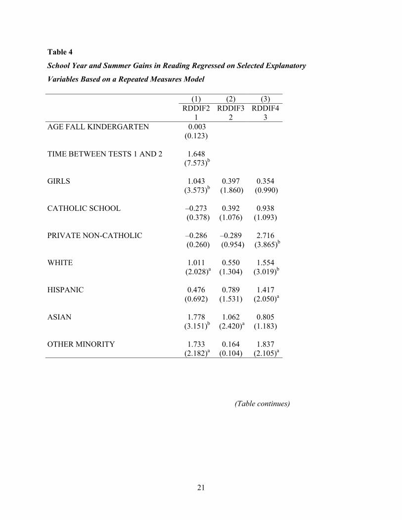
Table 4

School Year and Summer Gains in Reading Regressed on Selected Explanatory

Variables Based on a Repeated Measures Model

(1) (2) (3) RDDIF2

1 RDDIF3

2 RDDIF4

3 AGE FALL KINDERGARTEN 0.003 (0.123) TIME BETWEEN TESTS 1 AND 2 1.648 (7.573)b GIRLS 1.043 0.397 0.354 (3.573)b (1.860) (0.990) CATHOLIC SCHOOL –0.273 0.392 0.938 (0.378) (1.076) (1.093) PRIVATE NON-CATHOLIC –0.286 –0.289 2.716 (0.260) (0.954) (3.865)b

WHITE 1.011 0.550 1.554 (2.028)a (1.304) (3.019)b

HISPANIC 0.476 0.789 1.417 (0.692) (1.531) (2.050)a

ASIAN 1.778 1.062 0.805 (3.151)b (2.420)a (1.183) OTHER MINORITY 1.733 0.164 1.837 (2.182)a (0.104) (2.105)a

(Table continues)

21

Table 4 (continued)

(1) (2) (3) RDDIF2

1 RDDIF3

2 RDDIF4

3 HIGH SCHOOL GRADUATE 0.999 1.044 1.874 (2.419)a (2.813)b (2.936)b

SOME COLLEGE 1.443 1.392 2.004 (3.497)b (3.387)b (2.958)b

COLLEGE GRAD. OR HIGHER 1.496 1.912 2.799 (3.024)b (4.523)b (3.657)b

AGE SPRING KINDERGARTEN –0.010 (0.427) TIME BETWEEN TESTS 2 AND 3 0.273 (2.718)b AGE AT TIME OF 3RD TESING –0.104 (2.655)a

TIME BETWEEN TESTS 3 AND 4 0.412 (1.138) CONSTANT –2.572 2.258 19.077 (1.055) (1.306) (4.554)b

OBSERVATIONS 3,032 3,032 3,032 R-SQUARED 0.046 0.020 0.027

Note. Absolute value of t-statistics in parentheses. a significant at 5%. b significant at 1%.

22

This repeated measures scaling of the dependent variable yields a straightforward

interpretation of the raw score regression coefficients associated with the dummy variables

indicating group membership. For example, the regression weight associated with children who

come from families with at least one parent having a college degree or higher indicates a gain, on

average, of 1.496 score points more during the kindergarten year than children from homes with

neither parent having a high school degree (the contrast group). The regression weight associated

with this contrast is shown in bold in each of the succeeding tables. Differences in parent

education outweigh other demographic variables as predictors of the summer effect in reading.

Moreover, each successive increment in parent education is associated with greater and greater

gains during the summer, with a regression weight of 1.912 for children of college graduates

corresponding to the differential gain in score points for this group compared with children from

homes where neither parent finished high school. While this finding is consistent with the

summer effect literature, the comparable regression weight (college grad or higher) for the first

grade year is also significant and even higher (2.799), suggesting that even aside from the

differential growth during the summer, the gap would be steadily increasing during the

kindergarten and first grade years. In fact, all of the parental education subgroups showed this

pattern of increasing differentiation from the base group as they go from kindergarten through

first grade. Entwisle et al. (1997) found that their measure of socio-economic status was

unrelated to performance during the school year and negatively related to performance during the

summer months. The results here suggest that the gap between children from different parental

education backgrounds increases with each increment in parental education. That is, we have a

fan spread effect when the groups are defined by parental education level, with the children from

higher parental education levels growing faster both within and out of school in reading and

prereading skills. One difference between this study and that of Entwisle et al. (1997) is that they

began with first graders and the summer following the first grade. It is possible that as some

children proceed beyond first grade they are more likely to be moving from learning to read to

reading to learn and as a result they will have developed their comprehension skills to a level

where they can make additional gains on their own given a supportive educational environment.

Table 5 presents the analogous results for gains per month in mathematics. Inspection of

Table 5 indicates that there is no systematic differential de-acceleration among any of the

subpopulations during the summer months. In fact only the kindergarten year shows a significant

23

increase in rate of gain for the children with parents having a college degree or greater when

compared with those children having parents with less than a high school degree. There does not

seem to be any consistent pattern relating parental education level to rate of gains in or out of

school in mathematics.

Table 6 deals with the question of differential summer growth in reading from the

perspective of a Lag 1 analysis of covariance model. While Tables 4 and 5 used the repeated

measures correction for initial status, the analysis of covariance (ANCOVA) model will estimate

the correction for initial status from the data. Inspection of Table 4 suggests the same pattern of

an increasing gap in reading scores over time among children from different parental education

groups. This gap is widening during both school years as well as during the summer. The

estimated differential gain favoring the children of college educated parents during the

kindergarten year and the summer term is quite similar to that found in the repeated measures

model as reported in Table 4. This replication over different models occurs because the

adjustment factor for initial status in the ANCOVA model for kindergarten (.991 for reading

score at Time Point 1, in column 1) and summer (1.005 for reading score at Time Point 2, in

column 2) both turn out to be very close to 1, which is the adjustment factor for repeated

measures.

The adjustment for initial status for the first grade year in Table 6 is less than 1 (.857 for

reading score at Time Point 3, in column 3) and thus subgroup differences at the end of first

grade are only adjusted for a part of the differences that were present at entry to first grade.

Table 7 presents the analogous ANCOVA results for the mathematics scores. Inspection

of Table 7 shows the same trend of a growing achievement gap related to parents’ education. As

was the case for reading, the ANCOVA results in mathematics suggest that the gap favoring

children of parents with more education compared with children of parents with less education is

increasing over time, and increases at each increment of the parental education grouping.

24

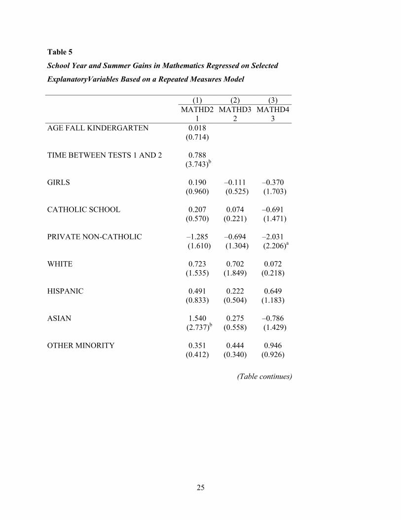
Table 5

School Year and Summer Gains in Mathematics Regressed on Selected

ExplanatoryVariables Based on a Repeated Measures Model

(1) (2) (3) MATHD2

1 MATHD3

2 MATHD4

3 AGE FALL KINDERGARTEN 0.018 (0.714) TIME BETWEEN TESTS 1 AND 2 0.788 (3.743)b GIRLS 0.190 –0.111 –0.370 (0.960) (0.525) (1.703) CATHOLIC SCHOOL 0.207 0.074 –0.691 (0.570) (0.221) (1.471) PRIVATE NON-CATHOLIC –1.285 –0.694 –2.031 (1.610) (1.304) (2.206)a WHITE 0.723 0.702 0.072 (1.535) (1.849) (0.218) HISPANIC 0.491 0.222 0.649 (0.833) (0.504) (1.183) ASIAN 1.540 0.275 –0.786 (2.737)b (0.558) (1.429) OTHER MINORITY 0.351 0.444 0.946 (0.412) (0.340) (0.926)

(Table continues)

25

Table 5 (continued)

(1) (2) (3) MATHD2

1 MATHD3

2 MATHD4

3 HIGH SCHOOL GRADUATE 0.430 0.220 –0.051 (1.319) (0.568) (0.106) SOME COLLEGE 1.101 0.247 0.435 (2.846)b (0.653) (0.843) COLLEGE GRAD. OR HIGHER 1.121 0.642 –0.148 (2.249)a (1.526) (0.284) AGE SPRING KINDERGARTEN 0.001 (0.065) TIME BETWEEN TESTS 2 AND 3 0.248 (2.746)b AGE AT TIME OF 3RD TESTING –0.100 (4.252)b TIME BETWEEN TESTS 3 AND 4 0.472 (1.809) CONSTANT 0.700 2.728 15.324 (0.310) (1.529) (5.369)b OBSERVATIONS 3,032 3,032 3,032 R-SQUARED 0.023 0.011 0.030

Note. Absolute value of t-statistics in parentheses. a significant at 5%. b significant at 1%.

26

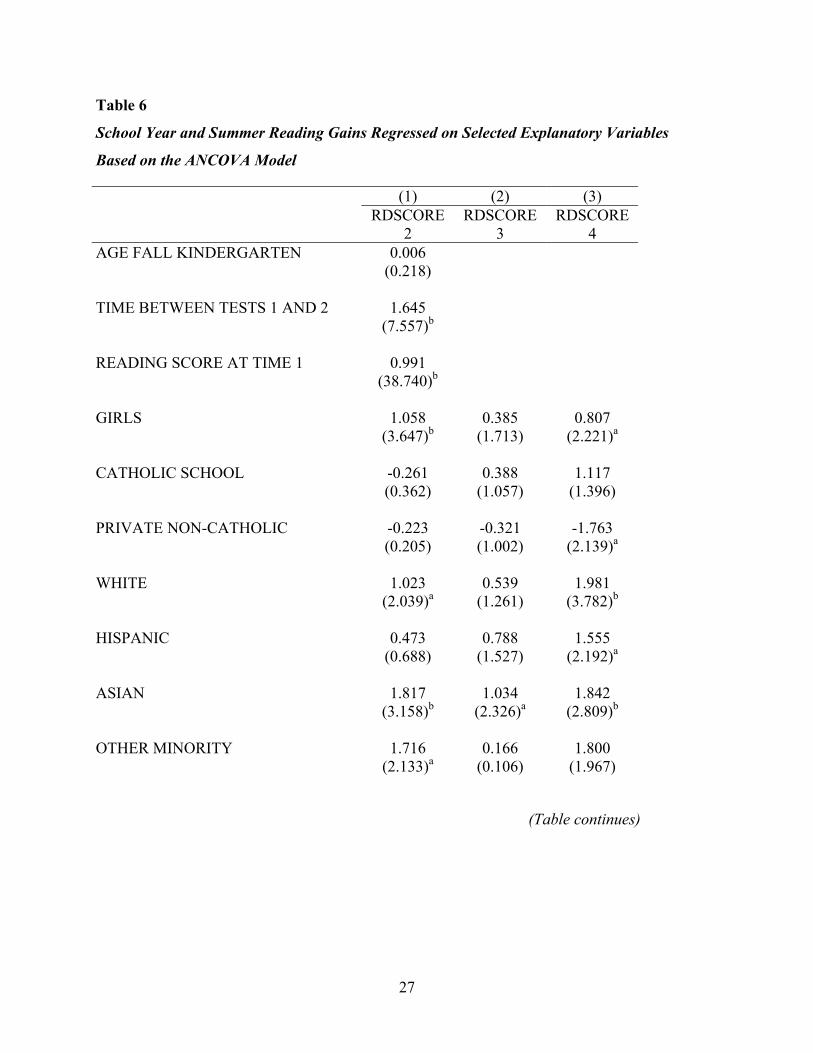
Table 6

School Year and Summer Reading Gains Regressed on Selected Explanatory Variables

Based on the ANCOVA Model

(1) (2) (3) RDSCORE

2 RDSCORE

3 RDSCORE

4 AGE FALL KINDERGARTEN 0.006 (0.218) TIME BETWEEN TESTS 1 AND 2 1.645 (7.557)b READING SCORE AT TIME 1 0.991 (38.740)b GIRLS 1.058 0.385 0.807 (3.647)b (1.713) (2.221)a CATHOLIC SCHOOL -0.261 0.388 1.117 (0.362) (1.057) (1.396) PRIVATE NON-CATHOLIC -0.223 -0.321 -1.763 (0.205) (1.002) (2.139)a WHITE 1.023 0.539 1.981 (2.039)a (1.261) (3.782)b HISPANIC 0.473 0.788 1.555 (0.688) (1.527) (2.192)a ASIAN 1.817 1.034 1.842 (3.158)b (2.326)a (2.809)b OTHER MINORITY 1.716 0.166 1.800 (2.133)a (0.106) (1.967)

(Table continues)

27

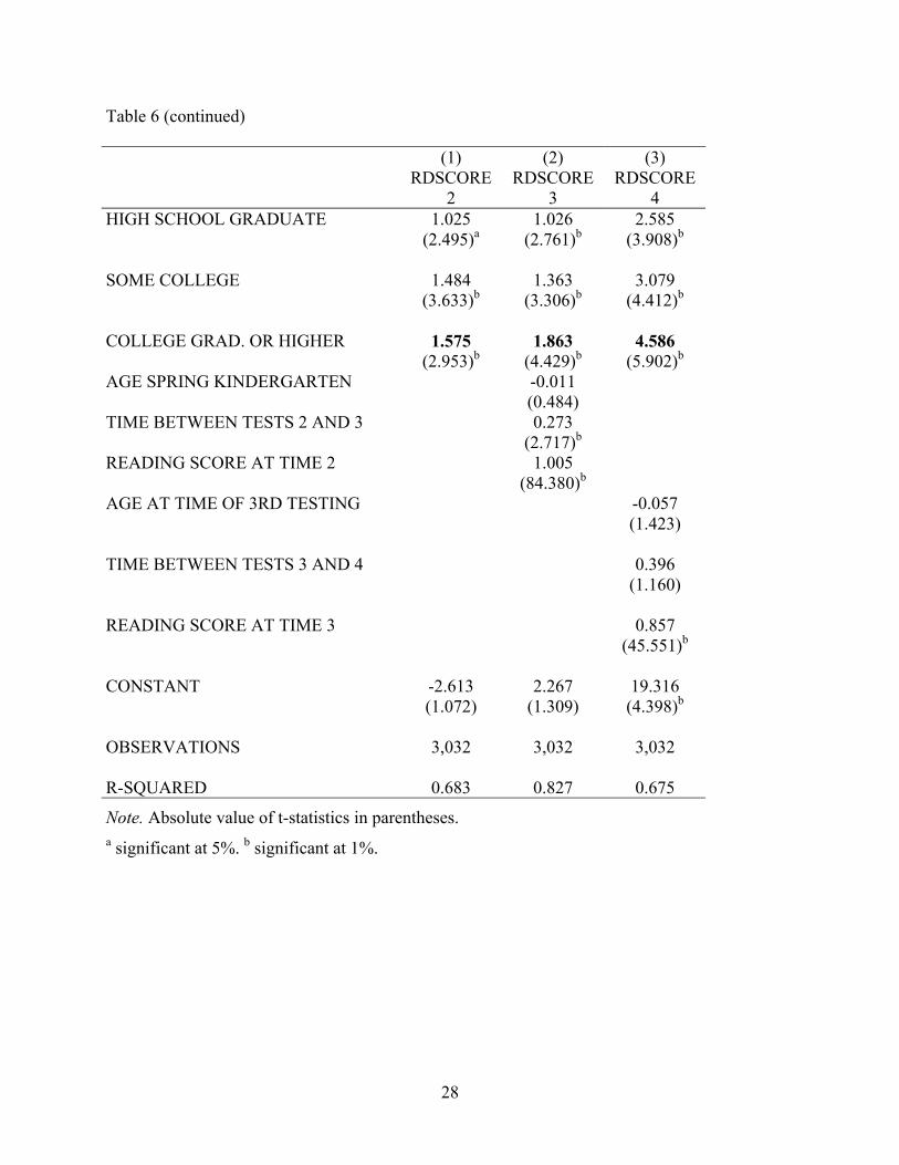
Table 6 (continued) (1) (2) (3) RDSCORE

2 RDSCORE

3 RDSCORE

4 HIGH SCHOOL GRADUATE 1.025 1.026 2.585 (2.495)a (2.761)b (3.908)b SOME COLLEGE 1.484 1.363 3.079 (3.633)b (3.306)b (4.412)b COLLEGE GRAD. OR HIGHER 1.575 1.863 4.586 (2.953)b (4.429)b (5.902)b AGE SPRING KINDERGARTEN -0.011 (0.484) TIME BETWEEN TESTS 2 AND 3 0.273 (2.717)b READING SCORE AT TIME 2 1.005 (84.380)b AGE AT TIME OF 3RD TESTING -0.057 (1.423) TIME BETWEEN TESTS 3 AND 4 0.396 (1.160) READING SCORE AT TIME 3 0.857 (45.551)b CONSTANT -2.613 2.267 19.316 (1.072) (1.309) (4.398)b OBSERVATIONS 3,032 3,032 3,032 R-SQUARED 0.683 0.827 0.675

Note. Absolute value of t-statistics in parentheses. a significant at 5%. b significant at 1%.

28

Table 7

School Year and Summer Gains in Mathematics Regressed Selected Explanatory

Variables Based on the ANCOVA Model

(1) (2) (3) MSCL2 MSCL3 MSCL4 AGE FALL KINDERGARTEN 0.047 (1.723) TIME BETWEEN TESTS 1 AND 2 0.768 (3.604)b MATH SCORE 1 0.922 (34.671)b GIRLS 0.224 –0.024 –0.245 (1.121) (0.112) (1.254) CATHOLIC SCHOOLS 0.324 0.307 –0.269 (0.851) (1.005) (0.588) PRIVATE NON-CATHOLIC –0.878 –0.148 –1.250 (1.032) (0.325) (1.372) WHITE 0.945 1.194 1.104 (1.997) (3.238)b (3.927)b HISPANIC 0.554 0.402 1.020 (0.932) (0.987) (1.977) ASIAN 1.768 0.890 0.353 (2.988)b (1.994) (0.728) OTHER MINORITY 0.336 0.461 1.080 (0.426) (0.330) (1.700)

(Table continues)

29

Table 7 (continued)

(1) (2) (3) MSCL2 MSCL3 MSCL4 HIGH SCHOOL GRADUATE 0.644 0.658 0.771 (2.038)a (1.611) (1.504) SOME COLLEGE 1.440 0.999 1.815 (3.775)b (2.560)a (3.297)b COLLEGE GRAD. OR HIGHER 1.732 1.880 2.182 (4.249)b (4.008)b (4.149)b AGE SPRING KINDERGARTEN 0.056 (2.511)a TIMEE BETWEEN TESTS 2 AND 3 0.247 (2.921)b MATH SCORE 2 0.862 (53.868)b AGE AT TIME OF 3RD TESTING –0.009 (0.362) TIME BETWEEN TESTS 3 AND 4 0.456 (2.026)a MATH SCORE 3 0.759 (47.392)b CONSTANT –0.138 1.455 13.977 (0.061) (0.854) (4.880)b OBSERVATIONS 3,032 3,032 3,032 R-SQUARED 0.669 0.728 0.674

Note. Absolute value of t-statistics in parentheses. a significant at 5%. b significant at 1%.

30

Qualitative Differences in Reading Gain Scores in the First Grade

Children attending private non-Catholic schools and/or having more educated parents

enter kindergarten at a much higher level in reading, on average, than their counterparts in public

schools or with less educated parents. Subgroups with different average scale scores are making

their gains at different points on the reading scale, meaning that the gains in scale score points

are achieved by different groups mastering somewhat different material. Using the first grade

year data, children were sorted into two groups: those who were making their maximum gains at

Level 5 skills, comprehension of words in context, (coded 1) versus those who were making their

maximum gains at any of the four lower level proficiencies (coded 0). A logistic regression of

this 0-1 outcome on the demographic variables, including the school sectors, was carried out.

Table 8 presents the complete results of the logistic regression with the logistic regression

coefficients transformed to odds ratios for ease of interpretation. Inspection of Table 8 indicates

that the odds-ratio associated with the private non-Catholic school children is 2.34 (t = 3.77;

p = .00), meaning that these children are 2.34 times as likely as their public school counterparts

to be making their maximum gains in the higher level reading skill of beginning reading

comprehension during first grade.

In addition to gaining more than the boys on the overall scale, girls were 1.57 (t = 4.77,

p = .00) times more likely to be making their gains in Level 5 reading skills by the end of first

grade, as indicated by the logistic regression predicting whether or not the child is gaining in

Level 5 skills (beginning reading comprehension).

The extent of the relationship between parents’ educational background and their

children’s achievement gains on the more demanding reading tasks was even more extreme. It

was found that children from homes where at least one parent has a college degree or higher are

more than 8 times as likely (t = 8.05; p = .00) as children from a home where neither parent has a

high school degree to be making their largest gains on the Level 5 comprehension tasks. The

children with strong educational support systems (i.e., high parental educational levels) were not

only gaining more in terms of reading scale score points than their counterparts, but were making

their maximum gains on the higher level reading tasks.

Asian children were 3.28 (t = 4.09, p = .00) times as likely as Black children to be

making their gains in Level 5 reading comprehension skills, while White children were 1.86

31

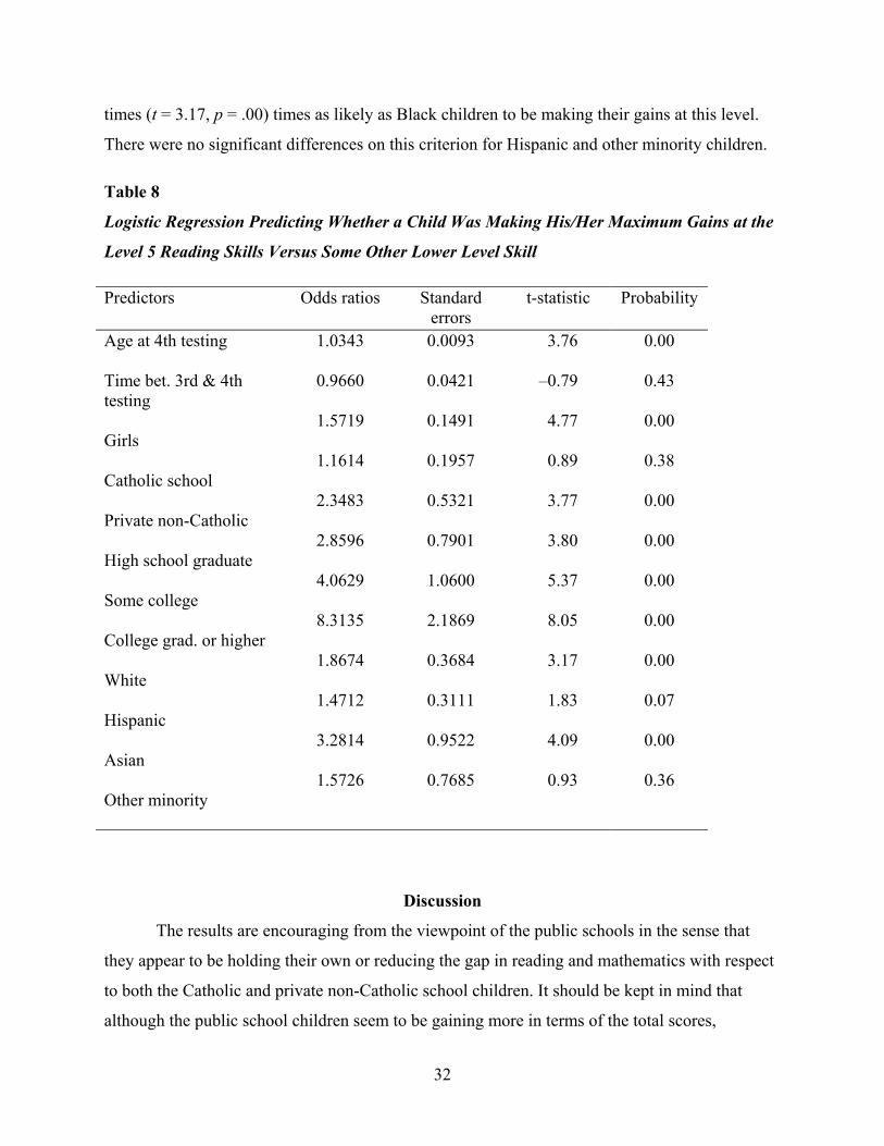
times (t = 3.17, p = .00) times as likely as Black children to be making their gains at this level.

There were no significant differences on this criterion for Hispanic and other minority children.

Table 8

Logistic Regression Predicting Whether a Child Was Making His/Her Maximum Gains at the

Level 5 Reading Skills Versus Some Other Lower Level Skill

Predictors Odds ratios Standard errors

t-statistic Probability

Age at 4th testing Time bet. 3rd & 4th

testing Girls Catholic school Private non-Catholic High school graduate Some college College grad. or higher White Hispanic Asian Other minority

1.0343

0.9660

1.5719

1.1614

2.3483

2.8596

4.0629

8.3135

1.8674

1.4712

3.2814

1.5726

0.0093

0.0421

0.1491

0.1957

0.5321

0.7901

1.0600

2.1869

0.3684

0.3111

0.9522

0.7685

3.76

–0.79

4.77

0.89

3.77

3.80

5.37

8.05

3.17

1.83

4.09

0.93

0.00

0.43

0.00

0.38

0.00

0.00

0.00

0.00

0.00

0.07

0.00

0.36

Discussion

The results are encouraging from the viewpoint of the public schools in the sense that

they appear to be holding their own or reducing the gap in reading and mathematics with respect

to both the Catholic and private non-Catholic school children. It should be kept in mind that

although the public school children seem to be gaining more in terms of the total scores,

32

particularly during the first grade year, compared with the private non-Catholic school children,

the public school children started out much lower on the scales at entry to kindergarten. As a

result, many public school children, by the end of the first grade year, are gaining in skills

measured in the middle of the scale that deal primarily with reading mechanics, while the private

non-Catholic school children are making their gains at the upper end of the scale, which is more

focused on beginning reading comprehension. In other words, there are qualitative differences in

gains between the public and private school children. As ECLS-K data becomes available for

grades 3 and 5, where the emphasis of the reading assessments is on comprehension of reading

passages rather than prereading mechanics and sentence comprehension, it will be interesting to

see if the public school children can maintain the same accelerated growth that seemed to

characterize their first grade year.

Children who are making their maximum gains during first grade in Level 5 skills

(beginning reading comprehension) are likely to be moving from the learning to read mode to the

reading to learn mode much earlier than their less advanced counterparts. One might expect these

better readers to begin to separate themselves from the others in other subject matter areas where

reading can be used as a tool for learning. It is also likely that they will be able to

disproportionately increase their gains over the summer months in the succeeding school years.

While the between school sector variation decreased from the time of entry to

kindergarten to spring first grade in both reading and mathematics, variation between parental

education groups and between ethnic groups increased over the same time period. This

phenomenon was more pronounced in the reading domain than in mathematics and for the

parental education groups than the ethnic groups.

Black children started kindergarten significantly below White children in both reading

and mathematics and had significantly lower growth rates than White children in both areas. This

is unfortunate. One would hope that formal schooling might reduce the gap between the

traditionally economically disadvantaged groups and the majority group. The higher correlations

between slopes and intercepts for reading compared with mathematics, at both the school and

child levels, suggest that it may be more important for later growth to come to kindergarten

better prepared in reading than is the case in mathematics. This would suggest that, in reading at

least, intensive preschool emphasis on prereading and reading mechanics might help reduce the

gap in the later growth rates between the disadvantaged and advantaged child.

33

Girls entered kindergarten with greater prereading and reading skills than did the boys.

They also had somewhat better mathematics skills at entry to kindergarten. While girls continued

to grow faster than boys in reading during the first two years of schooling, there was no

significant difference in their growth rates in mathematics. Girls in the first grade were twice as

likely as boys to be making their gains at the highest reading level, beginning reading

comprehension. Thus girls are not only growing faster than boys on the overall reading scale,

they are also making their gains on the more difficult reading tasks.

The finding that the interaction of the treatment (schooling) and differing parental

education levels led to an increased fan spread effect, particularly in reading, is quite important.

Children of highly educated parents had less de-acceleration in their growth rates during the

nontreatment (summer) period, and greater acceleration during the school years, when

compared with children of less educated parents. This greater acceleration in reading skills

during the school year as compared with summer gains for children of more highly educated

parents runs counter to much of the summer gains literature, that is, Entwisle and Alexander

(1992) and Entwisle et al. (1997). One possible reason for this is that these studies did not look at

the summer effects between kindergarten and first grade. Other possibilities might be that their

measurement instruments may have had ceiling effects. At any rate, if this nonadditivity

continues in the later grades, the reading scores of children from different parental education

groups will become even more disparate. This suggests that the presence of a strong educational

support system in the home is particularly effective in enhancing growth in the first two years of

schooling.

Conclusions

Reading and mathematics gains were relatively large for all subpopulations, but there

remained substantial differences in the rates of growth among both individuals and

subpopulations. Subpopulations from different demographic backgrounds typically entered

kindergarten with significant differences in their level of preparation in both the reading and

mathematics domains. In some cases these disparities were reduced, while in other cases the

disparities remained the same or even increased.

Mean gains during the school year typically exceeded a full standard deviation in both

reading and mathematics. Gains continued over the summer in both reading and mathematics but

at a reduced rate. With respect to gender differences, girls began kindergarten performing better

34

than boys in both reading and mathematics. In reading, girls also showed higher growth rates

than boys but there was no difference between the gender groups in growth rates in mathematics.

Public school children entered kindergarten performing significantly below children

entering Catholic and non-Catholic private schools in both reading and mathematics. This entry

deficit was particularly pronounced for the public versus private non-Catholic contrast. However,

the gap in reading performance between children in public compared with private non-Catholic

schools at entry to kindergarten was significantly reduced by the spring of first grade. Much of

this reduction resulted from a more highly accelerated growth rate for public school children in

the first grade. A similar pattern was found in mathematics. The gap in reading performance

between private non-Catholic school children and Catholic school children was also significantly

decreased by spring of first grade. The gap in mathematics performance found at entry to

kindergarten between private non-Catholic and Catholic school children was entirely erased by

spring of first grade. If the public schools are failing in their teaching role, it does not seem to be

happening during the first two years of schooling.

There were relatively large differential growth rates in reading performance for

subpopulations based on parental education. This differential growth rate in favor of children

from families with highly educated parents was evident over both the summer months and the

school year. The gap that remains at the end of first grade between children of highly educated

parents versus those from less educated families is the sum of initial differences at entry to

kindergarten and differential growth rates during both the summer and the two school years.

In terms of ethnic group membership, Asian and to a lesser extent White and Hispanic

children all showed significantly greater linear growth rates in reading than did the Black

children. Hispanic, Asian, and White children all had significantly greater linear growth rates in

mathematics than did Black children.

In terms of the quality of the gains, while the private non-Catholic school children gained

less than the public school children in terms of total scale points, they were more than twice as

likely to be gaining in their reading comprehension skills as opposed to the more basic reading

mechanics skills. Children from homes having a parent with a college degree or greater were

more than eight times as likely as children from homes without a high school graduate parent to

be gaining in that part of the scale dealing with beginning reading comprehension.

35

References

Bryk, A. S., & Raudenbush, S. W. (1992). Hierarchical linear models, applications and data

analysis methods. Newbury Park, CA: Sage.

Campbell, D. T., & Earlenbacher, A. E. (1970). How regression artifacts in quasi-experimental

evaluations can mistakenly make compensatory education look harmful. In J. Hellmuth

(Ed.), Disadvantaged child: Vol. 3. Compensatory education: A national debate. New

York: Brunner/Mazel.

Cooper, H., Nye, B., Charlton, K., Lindsey, J., & Greathouse, S. (1996). The effect of summer

vacation on achievement test scores: A narrative and meta-analytic review. Review of

Educational Research, 66, 227-268.

Entwisle, D. R., & Alexander, K. L. (1992). Summer setback: Race, poverty, school

composition, and mathematics achievement in the first two years school. American

Sociological Review, 57, 72-84.

Entwisle, D. R., & Alexander, K. L. (1994). Winter setback: The racial composition of schools

and learning to read. American Sociological Review, 59, 446-460.

Entwisle, D. R., Alexander, K. L., & Olson, L. S. (1997). Children, schools and inequality.

Boulder, CO; Westview Press.

Goldstein, H. (1995). Multilevel statistical models (2nd ed.). London: Arnold.

Goldstein, H., et al. (1998). A user’s guide to MlwiN [Computer software manual]. London:

University of London, Institute of Education, Multi-level Models Project.

Heyns, B. (1998). Summer learning and the effects of schooling. New York: Academic Press.

Lord, F. M. (1980). Applications of item response theory to practical testing problems. Hillsdale,

NJ: Erlbaum.

National Center for Education Statistics. (2002, January). ECLS-K first grade public-use data

file. Washington, DC: Author. (NCES 2002-134)

Rock, D. A., & Pollack, J. M. (2002). A model-based approach to measuring cognitive growth in

pre-reading and reading skills during the kindergarten year (ETS RR-02-18). Princeton,

NJ: ETS.

Snijders, T., & Bosker, R. (1999). Multilevel analysis: An introduction to basic and advanced

multilevel modeling. London: Sage.

36