Munich Personal RePEc Archive

Assessing classical input output

structures with trade networks: A graph

theory approach

Halkos, George and Tsilika, Kyriaki

Department of Economics, University of Thessaly

July 2016

Online at https://mpra.ub.uni-muenchen.de/72511/

MPRA Paper No. 72511, posted 13 Jul 2016 05:45 UTC

1

Assessing classical input output structures with trade networks: A graph theory approach

George E. Halkos and Kyriaki D. Tsilika Laboratory of Operations Research,

Department of Economics, University of Thessaly

Abstract We present data structures from multiregional multisectoral trade activities from the perspective of networks. To illustrate our approach we make use of trade patterns taken from three classical input-output models. Unlike other conventional approaches by which networks statistics are evaluated, here, emphasis is given on recovering the structure architecture of interrelations in the input-output model. By self-explanatory visual outputs we display the interaction of the trading partners, the number of trade links and the density of interrelations. Connectivity and density are quantified by evaluating the node degrees. Our network approach traces the feedback loops among regions and activities. Some global structural properties are also examined. Programming in Mathematica allows for the creation of iterative schemes explaining aspects of the nature of trade and the evolution of spatial trading/production cycles in growing trading systems. Mathematica’s environment enables interactive visual schemes and infinite number of experiments. Keywords: Trade data visualization; trade networks; Mathematica-based computations; graph theory. JEL Codes: C63; C88; F10.

2

1. Introduction

Multi-region, multi-sector classical models are traditionally described in their

compact forms by recursive formulas and by using matrix notations (Batten and

Martellato 1985; Hitomi at al. 2000; Sargento 2009; Munroe et al. 2007; Wixted et al.

2006). Several papers even use snapshots of the associated trade patterns (Hitomi et

al. 2002; McNerney et al. 2013; Halkos and Tsilika, 2015, 2016).

Since the trade network representation has been proposed in the analysis of

trade interdependencies (see indicatively Smith and White 1992; McFadzean and

Tesfatsion, 1999; Wilhite 2001; Serrano et al., 2007; Garlaschelli and Loffredo, 2005;

Kim and Shin, 2002; McFadzean et al. 2001; Amman et al. 2003; Alkemade et al.

2002), a network approach using elements from graph theory in Mathematics can

restore structural information embodied in their topology (Chow, 2013; Fagiolo et al.,

2008; Fagiolo et al., 2013; Wei and Liu 2012, Benedictis and Tajoli, 2011;

Garlaschelli & Loffredo, 2005).

Graph models have been deeply integrated into the input-output analysis and

were treated between others by Studer et al. (1984), Olsen (1992), Lantner and

Carluer (2004), McNerney (2009), Blöchl et al. (2011), Fedriani and Tenorio (2012),

Garcia Muñiz (2013), McNerney et al. (2013), Montresora and Marzettib (2009),

Cerina et al. (2015). Kaveh (2013) among others, having considered a great variety of

applications using graphs, highlights graphs’ contribution in representing a system so

that its topology can clearly be understood.

In this conceptual direction, multiregional input-output models are depicted as

graphs made up of vertices (also called nodes) and edges, representing traders and

trade links. A graph G={V,E} consists of a set of vertices V and a set of edges E.

3

Each vertex V stands for a regional activity (or sector or industry). Edges E represent

significant trade relationships.

To make theory into computational practice, classical trade models proposed

by Isard (1951), Chenery, Moses (Chenery et al. 1953, Moses 1955), Leontief (1953),

Riefler and Tiebout (Riefler and Tiebout 1970) are employed. We create a three-

paradigm presentation that allows for a variety of extensions to the whole IO

framework. Computations and graph modelling are performed in the environment of

one of the most popular computer algebra systems (CASs), Mathematica1. Our

programming ideas result in automatic creation of graphs of interregional intersectoral

input-output models, with the only input required be the number of regions and the

number of sectors. The evaluation of certain graph metrics for increasing network

sizes provides information for the network formation and evolution. Graph-based

classification and its practical interpretation set directions for policy making.

All computer codes are given in section 3, being accesible to the wide community

of Mathematica users. Section 2 of the paper briefly presents the mathematical

framework used and, section 4 concludes the paper.

2. Basic notions and fomulations

Assuming m regions and n sectors in interregional trade models, nm×nm

intersectoral and interregional trade flows occur. Technical coefficient matrix T is a

block matrix composed by nm×nm elements with 2m submatrices klT containing the

coefficients for n traded commodities. In the general case of m regions and n sectors,

matrix T has the following sub-matrix structure:

1 Mathematica software is tradable from Wolfram Research, Inc.

4

mmmm

m

m

TTT

TTTTTT

T

21

22221

11211

(1)

klT is an n× n matrix. The coefficient klijt indicates the fraction of the total

production of sector i supplied to the jth sector in region l that has produced and

shipped from region k.

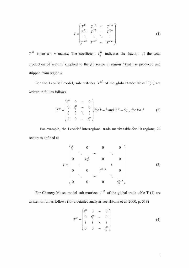
For the Leontief model, sub matrices klT of the global trade table T (1) are

written in full as follows

lk

t

tt

T

kln

kl

kl

kl

for ,

00

0000

2

1

and nnkl OT for k l (2)

Par example, the Leontief interregional trade matrix table for 10 regions, 26

sectors is defined as

10,1026

10,101

1,126

1,11

000

000

000

000

t

t

t

t

T

(3)

For Chenery-Moses model sub matrices klT of the global trade table T (1) are

written in full as follows (for a detailed analysis see Hitomi et al. 2000, p. 518)

kln

kl

kl

kl

t

tt

T

00

0000

2

1

(4)

5

As similar example, the Chenery-Moses interregional trade matrix table for 10

regions, 26 sectors is defined as

10,1026

1,1026

10,101

1,101

10,126

1,126

10,11

1,11

00

00

00

00

tt

tt

tt

tt

T

(5)

For Riefler-Tiebout model sub matrices klT of the global trade table T defined

in (1) are written in full as follows

lk

ttt

tttttt

T

klnn

kln

kln

kln

klkl

kln

klkl

kl

for ,

21

22221

11211

and lk

t

tt

T

kln

kl

kl

kl

for ,

00

0000

2

1

(6)

where ti is the trade coefficient of sector i.

The Riefler-Tiebout interregional trade matrix table for 10 regions, 26 sectors is

defined as (Yamano and Hitomi 2005)

10,1026,26

10,101,26

1,1026

10,1026,1

10,101,1

1,101

10,126

1,126,26

1,11,26

10,11

1,126,1

1,11,1

0

0

0

0

ttt

ttt

ttt

ttt

T

(7)

From the network aspect, the numerical configuration of a network hinges on the

adjacency matrix A of a binary network. Its entries aij obey the rule:

6

otherwise 0

e of %1eor

,e of %1e if 1

i ijij

j ijij

ija (8)

where ije is the exports from i to j (Chow, 2013).

The adjacency matrix for a graph will have dimensions n×n, where n is the

number of vertices. A symmetric adjacency matrix results in an undirected graph. An

undirected edge is interpreted as two directed edges with opposite directions. In the

three models under study the associated adjacency matrices are symmetric.

Though much useful information for trading interactions is gained by matrix

representations and tabular visualization techniques, feedback loops2 and global

connectivity patterns are not obvious from a trade coefficient matrix or an adjacency

matrix. A sophisticated approach to measure the impact of loops and regional

feedbacks by Lantner and Carluer (2004) relies on matrix algebra and its application

requires several mathematical skills. In this study, computer output with dynamic

content is created to present the formation and evolution of trading patterns and

feedback loops, with images.

3. Computer codes / Illustrative examples

In graph theory terminology, two vertices (nodes) u and v form an edge of the

graph if {u,v}E. If {u,v}E implies that {v,u}E, then G is an undirected graph.

Otherwise it is a directed graph. The graphs presented in sections 3.1-3.3 are

undirected, since their associated adjacency matrices are symmetric.

2 The study and analysis of the interregional trade flows in interregional economic activities often reveal interregional and inter-activity linkages, referred to as «feedback loops» and/or spatial production cycles in interregional level (see also Sonis et al. 1993, 1995; Sonis and Hewings, 2001; Hitomi et al. 2002).

7

3.1 The case of Leontief model

Leontief interregional trade model having 3 regions with 4 sectors each is

presented by a graph consisting of 12 nodes {i, j}: the first index corresponds to the ith

region and the second index corresponds to the jth sector. The Leontief trade structure

results in a scheme with twelve vertices that are linked to themselves. This scheme

practically represents self-flows or transactions between firms of the same sector.

To create the Leontief trade model with 3 regions having 4 sectors each with

graphs, the codes in Mathematica are:

multileontiefmatrix[i_, j_] := ArrayFlatten[ Table[If[n == m, DiagonalMatrix[Table[1, {j}]], SparseArray[{}, {j, j}]], {n, i}, {m, i}]] AdjacencyGraph[Flatten[Table[{i, j}, {i, 1, 3}, {j, 1, 4}], 1],multileontiefmatrix[3, 4], VertexLabels -> "Name", ImagePadding -> 30]

By the aforementioned routine, a user could generate the adjacency graph of

any Leontief model, with the desired number of regions and sectors. The only input

that needs to be defined is the arguments [i, j] (i corresponds to the number of regions

8

and j corresponds to the number of sectors) of the multileontiefmatrix programmed

function within Mathematica’s matrix graph constructor AdjacencyGraph.

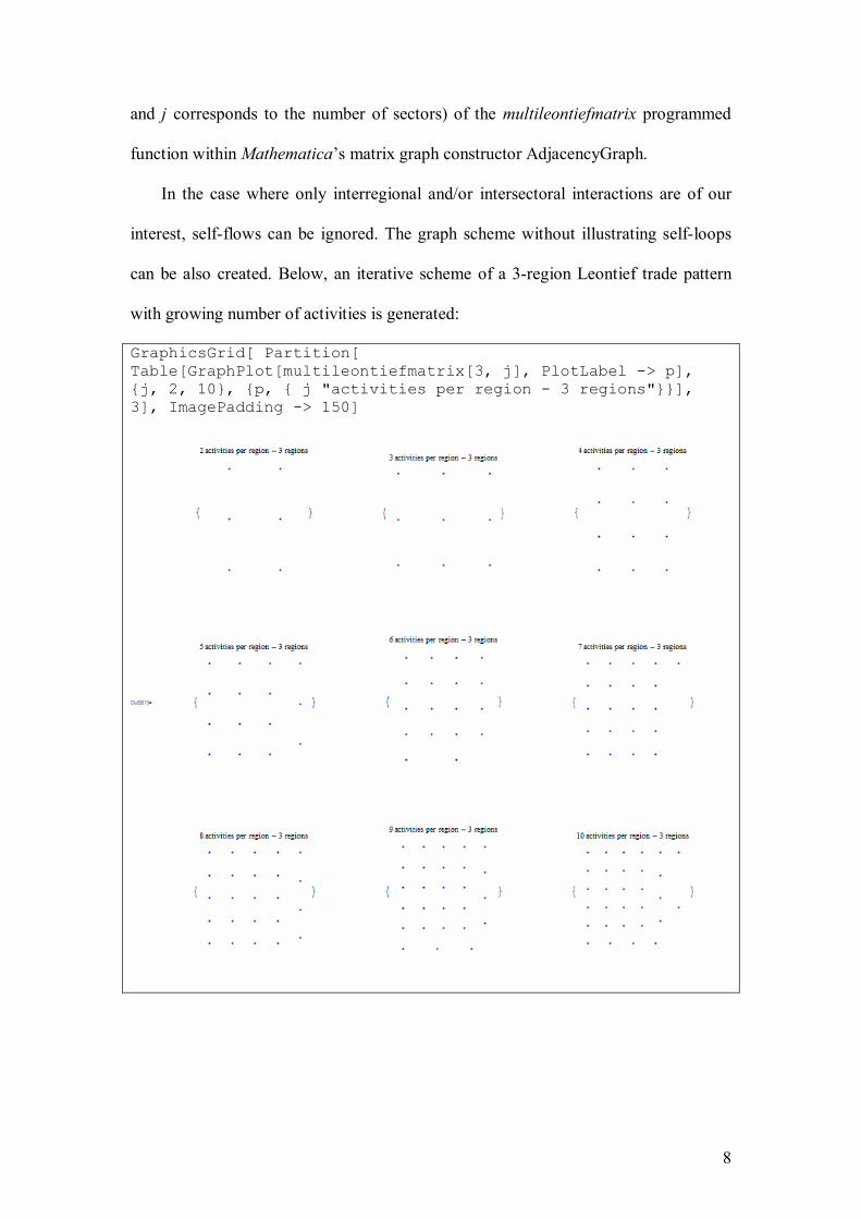
In the case where only interregional and/or intersectoral interactions are of our

interest, self-flows can be ignored. The graph scheme without illustrating self-loops

can be also created. Below, an iterative scheme of a 3-region Leontief trade pattern

with growing number of activities is generated:

GraphicsGrid[ Partition[ Table[GraphPlot[multileontiefmatrix[3, j], PlotLabel -> p], {j, 2, 10}, {p, { j "activities per region - 3 regions"}}], 3], ImagePadding -> 150]

9

A main measure in the study of social structures is the vertex (node) degree for

a vertex V which counts the number of edges incident to V. An edge is incident to a

vertex whether it is an in-edge or an out-edge.

In this study, we evaluate the degree of a node ni in order to quantify the trading

activity of the node. For the aforementioned Leontief example with 3 regions having 4

sectors each, the node degrees are calculated below:

VertexDegree[AdjacencyGraph[multileontiefmatrix[3, 4]]] {2, 2, 2, 2, 2, 2, 2, 2, 2, 2, 2, 2}

In the Leontief graph model all nodes have the same degree (each self-loop counts for

two trading activities).

Mathematica tests whether two Leontief graphs are isomorphic3. Roughly

speaking, graph isomorphism is a property to certify the structural equivalence of two

graphs (see also García Muñiz, 2013). By the following codes, Leontief graphs with

symmetric number of regions and sectors (i, j) are proved to be isomorphic:

IsomorphicGraphQ[AdjacencyGraph[multileontiefmatrix[3,5]], AdjacencyGraph[multileontiefmatrix[3, 5]]] True

3.2 The case of Chenery-Moses model

Chenery Moses interregional trade model having 3 regions with 4 sectors each

corresponds to a graph consisting of 12 nodes {i, j}: the first index corresponds to the

ith region and the second index corresponds to the jth sector. The undirected edges

stand for a bilateral trading activity. The graph model consists of four 3-regular

graphs4. In other words, four separate trading systems act together.

3 Two graphs are called isomorphic if they have the same number of nodes and the adjacency is preserved (Kaveh, 2013). 4 A graph is called regular if all its nodes have the same degree. If the degree is k then it is a k-regular graph (Diestel, 2000; Kaveh, 2013).

10

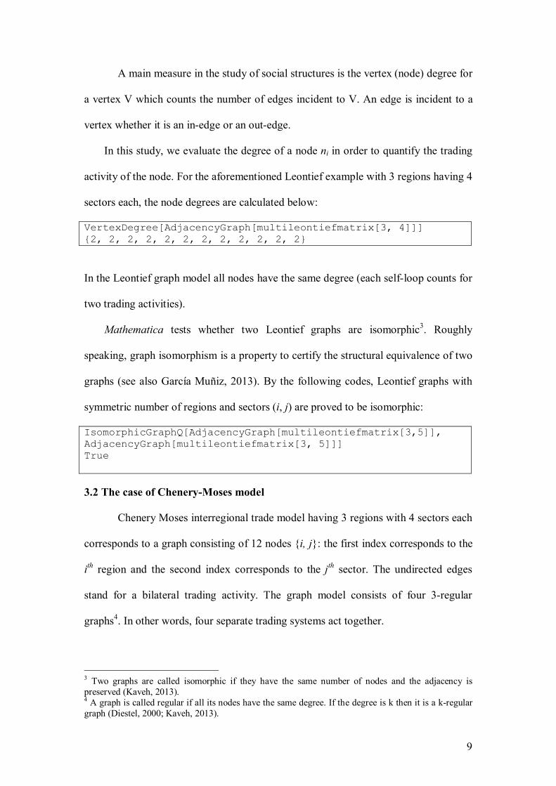
To create the Chenery-Moses trade model with 3 regions having 4 sectors each

with graphs, the codes in Mathematica are:

multicmmatrix[i_,j_]:=ArrayFlatten[Table[If[nm,DiagonalMatrix[Table[1,{j}]],DiagonalMatrix[Table[1,{j}]]],{n,i},{m,i}]] AdjacencyGraph[Flatten[Table[{i, j}, {i, 1, 3}, {j, 1, 4}], 1], multicmmatrix[3, 4], VertexLabels -> "Name", ImagePadding -> 30] The relevant output5 is

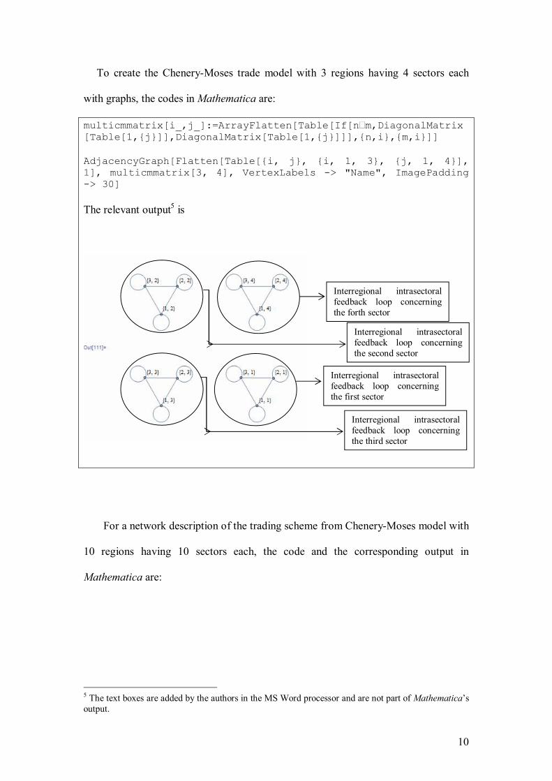
For a network description of the trading scheme from Chenery-Moses model with

10 regions having 10 sectors each, the code and the corresponding output in

Mathematica are:

5 The text boxes are added by the authors in the MS Word processor and are not part of Mathematica’s output.

Interregional intrasectoral feedback loop concerning the first sector

Interregional intrasectoral feedback loop concerning the forth sector

Interregional intrasectoral feedback loop concerning the second sector

Interregional intrasectoral feedback loop concerning the third sector

11

AdjacencyGraph[multicmmatrix[10, 10]]

Mathematica provides the choice to generate a graph without connecting self-

joined nodes (self-loops). The practical value of such a scheme is to present the

trading activities among different nodes. The dialog in Mathematica consists of the

following input and output:

GraphPlot[multicmmatrix[10, 10]]

12

A visual output with controllers added to the number of regions and the

number of sectors is presented in Figure 1. The selection of the number of regions and

sectors is made from a dedicated drop down list. The code to generate the dynamic

scheme is:

Manipulate[GraphPlot[multicmmatrix[regions, sectors], PlotLabel -> "Chenery Moses model"], {regions, Range[20]}, {sectors, Range[20]}, ControlType -> Automatic]

Figure 1: Snapshots from the dynamic output of Chenery Moses trading network

The codes below generate sequences of Chenery-Moses graphs, by following

an additive rule for the number of regions or the number of sectors (activities). The

automatic creation of an assigned title per graph, containing the exact number of

regions and sectors (activities), is also programmed. The images enable the user

realize the intensity of interactions when varying the number of regions (Figure 2) or

the number of sectors (Figure 3).

13

GraphicsGrid[Partition[Table[GraphPlot[multicmmatrix[i, 5], PlotLabel -> p], {i, 2, 10}, {p, {i "regions and 5 activities"}}], 3]]

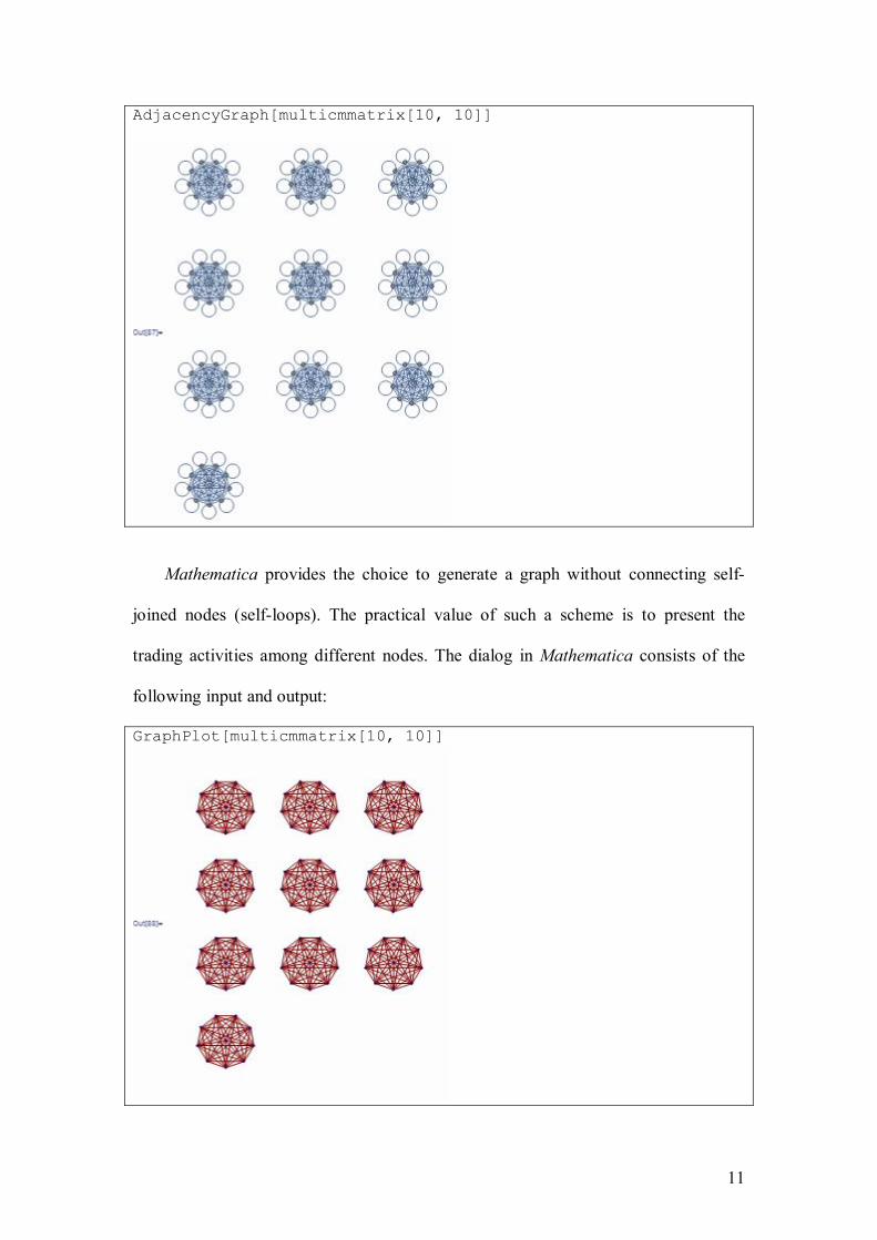
Figure 2: Mathematica output: Chenery-Moses trading network sequence with varying the number of regions GraphicsGrid[Partition[ Table[GraphPlot[multicmmatrix[5, j], PlotLabel -> p], {j, 2, 10}, {p, {j "activities per region - 5 regions"}}], 3]]

14

Figure 3: Mathematica output: Chenery-Moses trading network sequence with varying the number of activities

All graphical outputs presented can be reproduced for any case of Chenery-

Moses model, with the desired number of regions and sectors. The only input that

needs to be defined is the arguments [i, j] (i corresponds to the number of regions and

j corresponds to the number of sectors) of the multicmmatrix programmed function

within the routines.

To quantify the trading activity of a node we evaluate the degree of a node ni. For

the aforementioned Chenery-Moses example with 3 regions having 4 sectors each and

the example with 10 regions having 10 sectors each, the node degrees are calculated

15

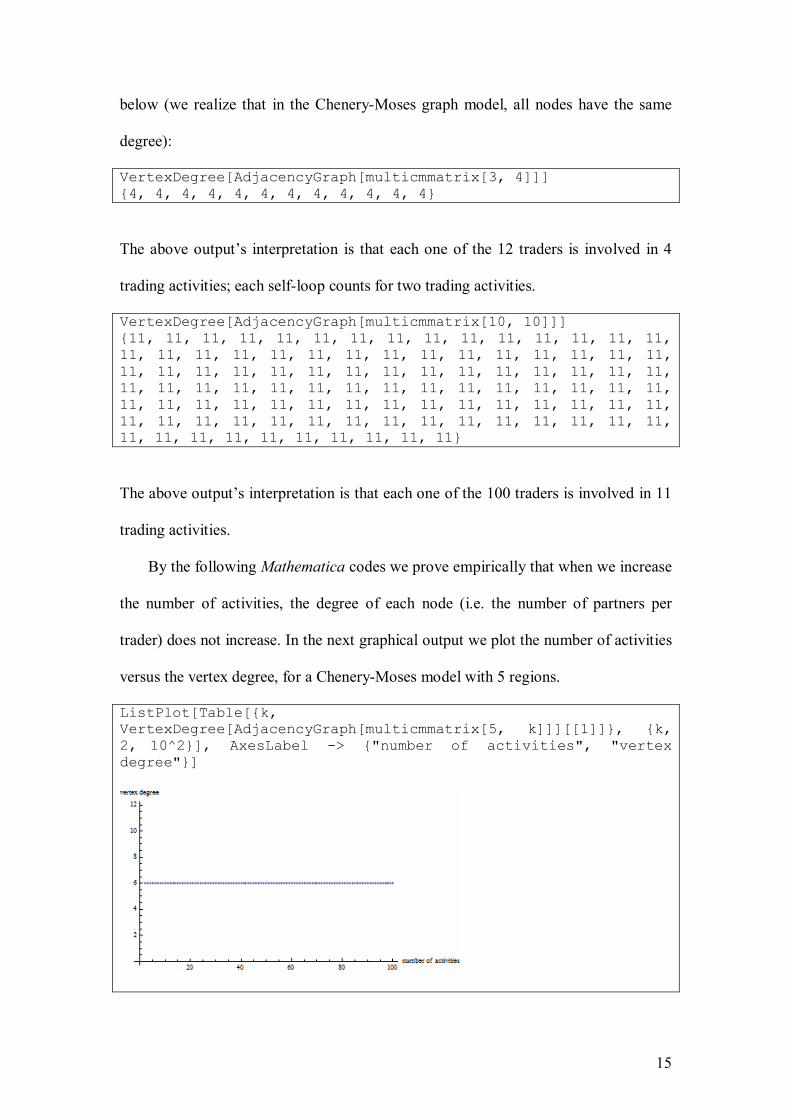
below (we realize that in the Chenery-Moses graph model, all nodes have the same

degree):

VertexDegree[AdjacencyGraph[multicmmatrix[3, 4]]] {4, 4, 4, 4, 4, 4, 4, 4, 4, 4, 4, 4}

The above output’s interpretation is that each one of the 12 traders is involved in 4

trading activities; each self-loop counts for two trading activities.

VertexDegree[AdjacencyGraph[multicmmatrix[10, 10]]] {11, 11, 11, 11, 11, 11, 11, 11, 11, 11, 11, 11, 11, 11, 11, 11, 11, 11, 11, 11, 11, 11, 11, 11, 11, 11, 11, 11, 11, 11, 11, 11, 11, 11, 11, 11, 11, 11, 11, 11, 11, 11, 11, 11, 11, 11, 11, 11, 11, 11, 11, 11, 11, 11, 11, 11, 11, 11, 11, 11, 11, 11, 11, 11, 11, 11, 11, 11, 11, 11, 11, 11, 11, 11, 11, 11, 11, 11, 11, 11, 11, 11, 11, 11, 11, 11, 11, 11, 11, 11, 11, 11, 11, 11, 11, 11, 11, 11, 11, 11}

The above output’s interpretation is that each one of the 100 traders is involved in 11

trading activities.

By the following Mathematica codes we prove empirically that when we increase

the number of activities, the degree of each node (i.e. the number of partners per

trader) does not increase. In the next graphical output we plot the number of activities

versus the vertex degree, for a Chenery-Moses model with 5 regions.

ListPlot[Table[{k, VertexDegree[AdjacencyGraph[multicmmatrix[5, k]]][[1]]}, {k, 2, 10^2}], AxesLabel -> {"number of activities", "vertex degree"}]

16

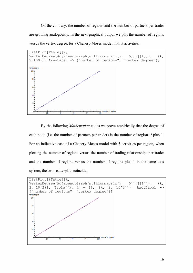
On the contrary, the number of regions and the number of partners per trader

are growing analogously. In the next graphical output we plot the number of regions

versus the vertex degree, for a Chenery-Moses model with 5 activities.

ListPlot[Table[{k, VertexDegree[AdjacencyGraph[multicmmatrix[k, 5]]][[1]]}, {k, 2,100}], AxesLabel -> {"number of regions", "vertex degree"}]

By the following Mathematica codes we prove empirically that the degree of

each node (i.e. the number of partners per trader) is the number of regions i plus 1.

For an indicative case of a Chenery-Moses model with 5 activities per region, when

plotting the number of regions versus the number of trading relationships per trader

and the number of regions versus the number of regions plus 1 in the same axis

system, the two scatterplots coincide.

ListPlot[{Table[{k, VertexDegree[AdjacencyGraph[multicmmatrix[k, 5]]][[1]]}, {k, 2, 10^2}], Table[{k, k + 1}, {k, 2, 10^2}]}, AxesLabel -> {"number of regions", "vertex degree"}]

17

Using a graph-based classification, the Chenery-Moses graph model with i-

regions is an i+1-regular graph.

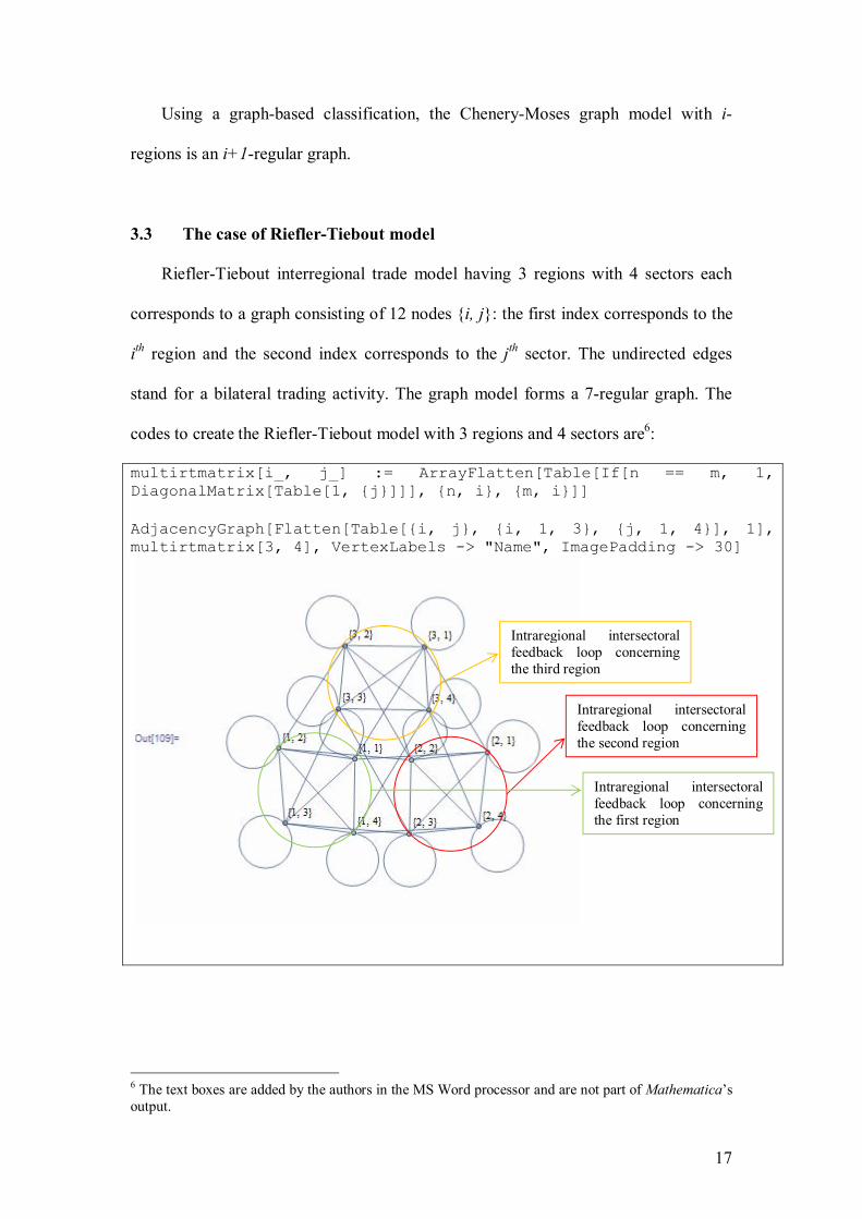
3.3 The case of Riefler-Tiebout model

Riefler-Tiebout interregional trade model having 3 regions with 4 sectors each

corresponds to a graph consisting of 12 nodes {i, j}: the first index corresponds to the

ith region and the second index corresponds to the jth sector. The undirected edges

stand for a bilateral trading activity. The graph model forms a 7-regular graph. The

codes to create the Riefler-Tiebout model with 3 regions and 4 sectors are6:

multirtmatrix[i_, j_] := ArrayFlatten[Table[If[n == m, 1, DiagonalMatrix[Table[1, {j}]]], {n, i}, {m, i}]] AdjacencyGraph[Flatten[Table[{i, j}, {i, 1, 3}, {j, 1, 4}], 1], multirtmatrix[3, 4], VertexLabels -> "Name", ImagePadding -> 30]

6 The text boxes are added by the authors in the MS Word processor and are not part of Mathematica’s output.

Intraregional intersectoral feedback loop concerning the second region

Intraregional intersectoral feedback loop concerning the first region

Intraregional intersectoral feedback loop concerning the third region

18

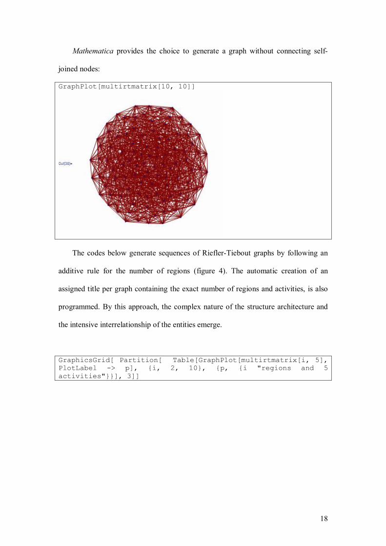
Mathematica provides the choice to generate a graph without connecting self-

joined nodes:

GraphPlot[multirtmatrix[10, 10]]

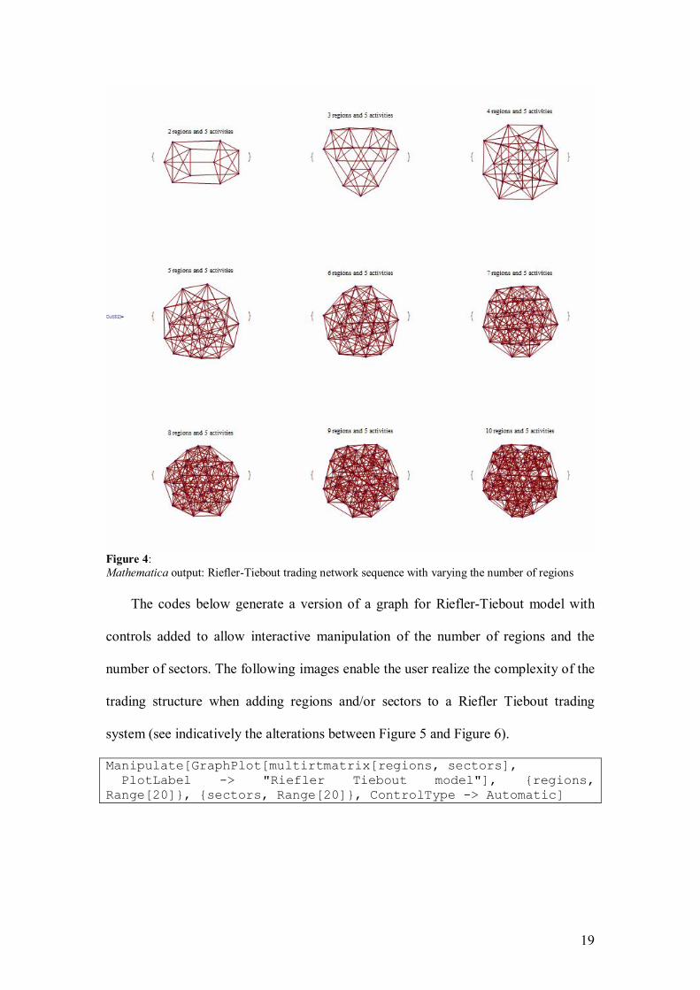
The codes below generate sequences of Riefler-Tiebout graphs by following an

additive rule for the number of regions (figure 4). The automatic creation of an

assigned title per graph containing the exact number of regions and activities, is also

programmed. By this approach, the complex nature of the structure architecture and

the intensive interrelationship of the entities emerge.

GraphicsGrid[ Partition[ Table[GraphPlot[multirtmatrix[i, 5], PlotLabel -> p], {i, 2, 10}, {p, {i "regions and 5 activities"}}], 3]]

19

Figure 4: Mathematica output: Riefler-Tiebout trading network sequence with varying the number of regions

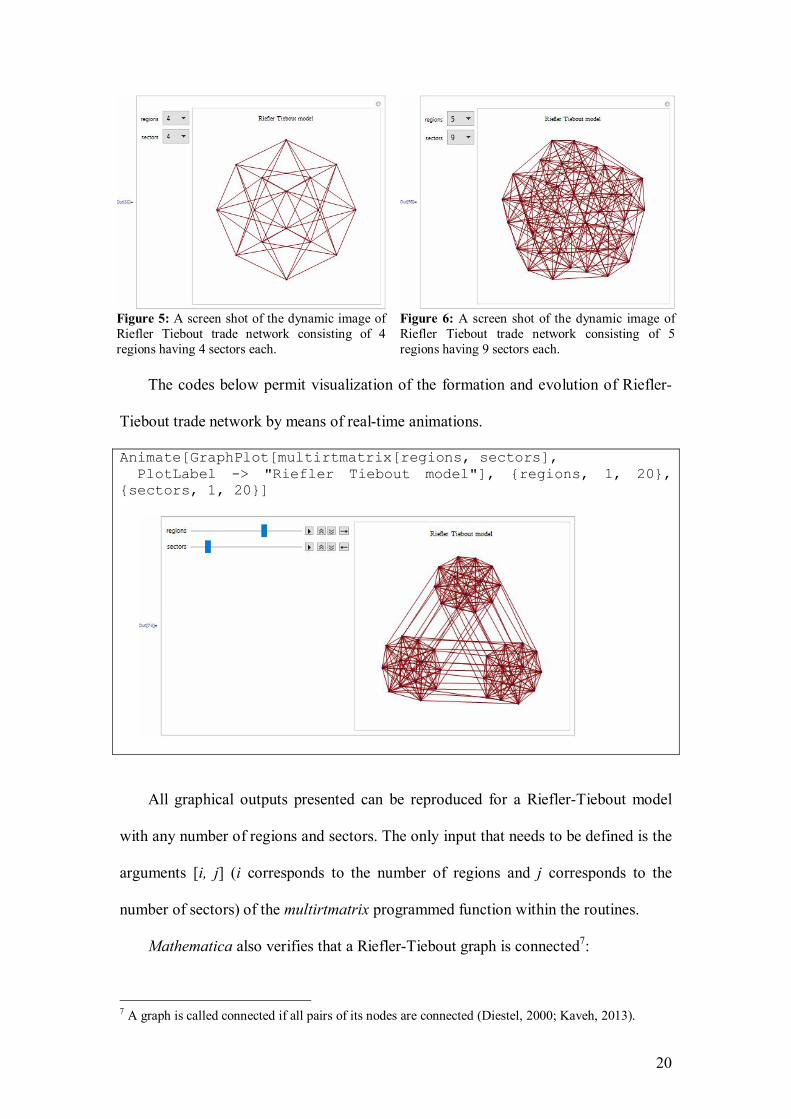
The codes below generate a version of a graph for Riefler-Tiebout model with

controls added to allow interactive manipulation of the number of regions and the

number of sectors. The following images enable the user realize the complexity of the

trading structure when adding regions and/or sectors to a Riefler Tiebout trading

system (see indicatively the alterations between Figure 5 and Figure 6).

Manipulate[GraphPlot[multirtmatrix[regions, sectors], PlotLabel -> "Riefler Tiebout model"], {regions, Range[20]}, {sectors, Range[20]}, ControlType -> Automatic]

20

Figure 5: A screen shot of the dynamic image of Riefler Tiebout trade network consisting of 4 regions having 4 sectors each.

Figure 6: A screen shot of the dynamic image of Riefler Tiebout trade network consisting of 5 regions having 9 sectors each.

The codes below permit visualization of the formation and evolution of Riefler-

Tiebout trade network by means of real-time animations.

Animate[GraphPlot[multirtmatrix[regions, sectors], PlotLabel -> "Riefler Tiebout model"], {regions, 1, 20}, {sectors, 1, 20}]

All graphical outputs presented can be reproduced for a Riefler-Tiebout model

with any number of regions and sectors. The only input that needs to be defined is the

arguments [i, j] (i corresponds to the number of regions and j corresponds to the

number of sectors) of the multirtmatrix programmed function within the routines.

Mathematica also verifies that a Riefler-Tiebout graph is connected7:

7 A graph is called connected if all pairs of its nodes are connected (Diestel, 2000; Kaveh, 2013).

21

ConnectedGraphQ[AdjacencyGraph[multirtmatrix[3, 5]]] True and performs graph matching. In Riefler-Tiebout case, graphs with symmetric number

of regions and sectors (i, j) are proved to be isomorphic:

IsomorphicGraphQ[AdjacencyGraph[multirtmatrix[3, 5]], AdjacencyGraph[multirtmatrix[5, 3]]] True

To quantify the trading activity of a node we evaluate the degree of a node ni. For

the aforementioned Riefler-Tiebout example with 3 regions having 4 sectors each and

the example with 10 regions having 10 sectors each, the node degrees are calculated

below (we realize that in the Riefler-Tiebout graph model all nodes have the same

degree):

VertexDegree[AdjacencyGraph[multirtmatrix[3, 4]]] {7, 7, 7, 7, 7, 7, 7, 7, 7, 7, 7, 7}

The above output’s interpretation is that each one of the 12 traders is involved in 7

trading activities; each self-loop counts for two trading activities.

VertexDegree[AdjacencyGraph[multirtmatrix[10, 10]]] {20, 20, 20, 20, 20, 20, 20, 20, 20, 20, 20, 20, 20, 20, 20, 20, 20, 20, 20, 20, 20, 20, 20, 20, 20, 20, 20, 20, 20, 20, 20, 20, 20, 20, 20, 20, 20, 20, 20, 20, 20, 20, 20, 20, 20, 20, 20, 20, 20, 20, 20, 20, 20, 20, 20, 20, 20, 20, 20, 20, 20, 20, 20, 20, 20, 20, 20, 20, 20, 20, 20, 20, 20, 20, 20, 20, 20, 20, 20, 20, 20, 20, 20, 20, 20, 20, 20, 20, 20, 20, 20, 20, 20, 20, 20, 20, 20, 20, 20, 20} The above output’s interpretation is that each one of the 100 traders is involved in 20

trading activities.

By the following Mathematica codes we prove empirically that the degree of

each node (i.e. the number of partners per trader) is the sum of the number of regions i

with the number of sectors j. For an indicative case of a Riefler-Tiebout model with 5

regions, when plotting the number of activities versus the number of partners per

22

trader and the number of regions versus the sum of regions and sectors in the same

axis system, the two scatterplots coincide.

ListPlot[{Table[{k, VertexDegree[AdjacencyGraph[multirtmatrix[5, k]]][[1]]}, {k, 2, 10^2}], Table[{k, 5 + k}, {k, 2, 10^2}]}, AxesLabel -> {"number of activities", "vertex degree"}]

Using a graph-based classification, the Riefler-Tiebout graph model with i-

regions and j-sectors is an i+j-regular graph.

4. Discussion and conclusions

Our computerized graph-based approach creates functions for network

description of the trading scheme for classical IO models. Our codes provide a

passage from tabular formats of mathematical formulation to graphical formats of

network analysis. Dedicated routines create visual versions of networks displaying

classical IO trade models with graphs. Static and dynamic images recover the global

structure of trade interactions. The proposed approach enables the user present,

understand and consider the impact of the model size on the intensity of trading

interactions and/or the density of the associated network.

In the technical context, the first step of our computational approach is

programming the adjacency matrix (the vertex–vertex adjacency matrix of the graph)

23

for every IO model used, being the required input in the upcoming codes for visual

outputs. In a second step, selected built-in Mathematica functions generate plots of

the associated graph. Graph drawing and graph programming commands and options

result in advanced schemes of trade representations. Quantitative results are obtained

by built-in Mathematica functions which evaluate metrics and test graph properties

for infinite cases of the classical models studied.

The main advantage of our schematic representation, compared with other

visualization techniques, is the focus on trade-cycle loops. The relative findings from

our illustrative examples bring out three different cases. The Leontief case study

reveals a trade structure with no trade-cycle loops among regions or among sectors

(only self-loops are traced). The Chenery-Moses case study reveals a global trade

network with a number of autonomous8 intrasectoral networks equal to the sectors of

the regions. There, interaction and connectivity involve part of the system (partial

interconnectedness). The Riefler-Tiebout case study reveals a trading system

equivalent to one compact trade network (one connected graph) with trade ties among

most its entities. In this case, interaction and connectivity involve the whole system

(global interconnectedness).

The practical interpretation of the node degree results is that in Chenery-

Moses model an increase in the number of activities does not affect the network

density and gives no benefit to any trader of the system. On the contrary, an increase

in the number of regions seems in benefit of all traders, since their trading activity

increases. In Riefler-Tiebout model, an increase in the number of both parameters,

regions and activities, rises the network density. These results, along with the iterative

8 The set SN is autonomous if and only if there are not any edges from the vertex of N\S to a vertex of S (Fedriani and Tenorio, 2012).

24

schemes which perform experiments with a comparative character, set some

directions for policy making.

Leontief and Riefler-Tiebout models with symmetric number of regions and

sectors (i.e. models with i-regions and j-sectors and models with j-regions and i-

sectors) are isomorphic. This information permits the decision maker to manage the

number of regions and sectors properly in order to control the network’s connectivity

and the distribution of commodities.

Last, the fact that the trade patterns of the three models under study result in

regular graphs, means that traders of the same model deal with the same consequences

coming from alterations in the network’s density.

25

Appendix

The adjacency matrix associated with each one of the I-O models under study,

is generated in Mathematica by dedicated programmed functions. The codes in

Mathematica are given below. In each matrix, entry 1 is used to indicate the fact that

two sectors are related and 0 that they are not.

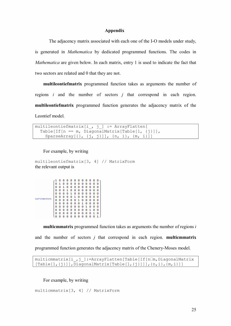
multileontiefmatrix programmed function takes as arguments the number of

regions i and the number of sectors j that correspond in each region.

multileontiefmatrix programmed function generates the adjacency matrix of the

Leontief model.

multileontiefmatrix[i_, j_] := ArrayFlatten[ Table[If[n == m, DiagonalMatrix[Table[1, {j}]], SparseArray[{}, {j, j}]], {n, i}, {m, i}]]

For example, by writing

multileontiefmatrix[3, 4] // MatrixForm the relevant output is

multicmmatrix programmed function takes as arguments the number of regions i

and the number of sectors j that correspond in each region. multicmmatrix

programmed function generates the adjacency matrix of the Chenery-Moses model.

multicmmatrix[i_,j_]:=ArrayFlatten[Table[If[nm,DiagonalMatrix[Table[1,{j}]],DiagonalMatrix[Table[1,{j}]]],{n,i},{m,i}]]

For example, by writing

multicmmatrix[3, 4] // MatrixForm

26

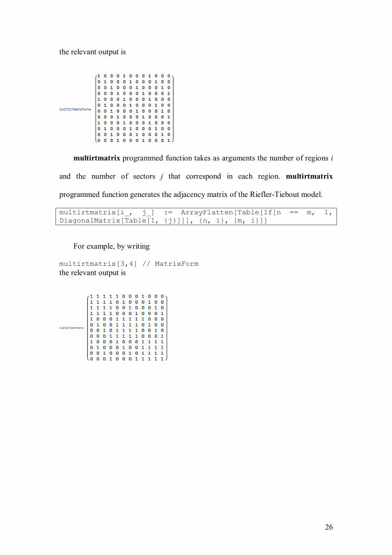
the relevant output is

multirtmatrix programmed function takes as arguments the number of regions i

and the number of sectors j that correspond in each region. multirtmatrix

programmed function generates the adjacency matrix of the Riefler-Tiebout model.

multirtmatrix[i_, j_] := ArrayFlatten[Table[If[n == m, 1, DiagonalMatrix[Table[1, {j}]]], {n, i}, {m, i}]]

For example, by writing

multirtmatrix[3,4] // MatrixForm the relevant output is

27

References Alkemade, F., Amman, H. & La Poutre, J., A. (2002). The Role of Information in an Electronic Trade

Network. Computing in Economics and Finance, 376, Society for Computational Economics. Accessible at: https://ideas.repec.org/p/sce/scecf2/376.html

Amman, H., Alkemade, F., & La Poutre, H. (2003). Intermediaries in an Electronic Trade Network. Computing in Economics and Finance, 6, Society for Computational Economics. Accessed from: https:// ideas.repec.org/p/sce/scecf3/6.html

Batten, D & Martellato, D. (1985). Classical versus modern approaches to interregional input-output analysis. The Annals of Regional Science, 19(3), 1-15. DOI: 10.1007/BF01294827

Benedictis, L.D. & Tajoli, L. (2011). The World Trade Network. The World Economy, 34(8), 1417-54.

Blöchl, F., Theis, F. J., Vega-Redondo, F. and Fisher, E. O’N., (2011). Vertex centralities in input-output networks reveal the structure of modern economies. Physical Review E, 83(4), 046127.

Chenery, H., Clark, P. G., & Cao Pinna, V. (1953). The structure and growth of the Italian economy, Rome: U.S. Mutual Security Agency.

Cerina F., Zhu Z., Chessa A., Riccaboni M. (2015), World Input-Output Network. PLoS ONE 10(7): e0134025. doi:10.1371/journal.pone.0134025

Chow, W. (2013) An Anatomy of the World Trade Network. Available at http://www.hkeconomy.gov.hk/en/pdf/An%20Anatomy%20of%20the%20World%20Trade%20Network%20%28July%202013%29.pdf

Diestel, R., (2000). Graph Theory. Electronic Edition 2000. Springer-Verlag, New York.

Fagiolo, G., Reyes, J. and Schiavo, S. (2008), On the topological properties of the world trade web: A weighted network analysis, Physica A: Statistical Mechanics and its Applications, 387(15), 3868-3873, http://dx.doi.org/10.1016/j.physa.2008.01.050.

Fagiolo, G., Squartini, T. & Garlaschelli, D., (2013). Null models of economic networks: the case of the world wide web. Journal of Economic Interaction and Coordination, 8(1), 75-107.

Fedriani, E. M. and Tenorio, Á. F. (2012), Simplifying the input–output analysis through the use of topological graphs, Economic Modelling, 29(5), 1931-1937, http://dx.doi.org/10.1016/j.econ mod.2012.06.006

Garlaschelli, D. & Loffredo, M.I. (2005). Structure and evolution of the world trade network. Physica A: Statistical Mechanics and its Applications, 355(1), 138-44.

García Muñiz, A.S. (2013), Input–output research in structural equivalence: Extracting paths and similarities, Economic Modelling, 31, 796-803, http://dx.doi.org/10.1016/j.econ mod.2013.01.016

Halkos, G.E. & Tsilika, K. D. (2015). A Dynamic Interface for Trade Pattern Formation in Multi-regional Multi-sectoral Input-Output Modeling. Computational Economics, 46(4), 671-681. DOI 10.1007/s10614-014-9466-3.

Halkos, G.E. & Tsilika, K. D. (2016). Trading Structures for Regional Economies in CAS Software. Computational Economics, DOI 10.1007/s10614-015-9515-6.

Hitomi, K., Okuyama, Y., Hewings, G. J. D., & Sonis M. (2000). The role of interregional trade in generating change in the regional economies of Japan, 1980#1990. Economic Systems Research, 12(4), 515-537.

Hitomi, K., Hewings, G. J. D., Yamano, N. and Ohkawara, T. (2002). Hollowing Out Process in Regional Economy: an Interregional Input-Ouput Analysis, CRIEPI REPORT Y01014. Available at http://criepi.denken.or.jp/en/publications/criepi_report/

Isard, W. (1951). Interregional and regional input-output analysis: A model of a space economy. The Review of Economics and Statistics, 33, 318-328.

Kaveh, A. (2013). Optimal Analysis of Structures by Concepts of Symmetry and Regularity. Springer-Verlag, Wien.

28

Kim, S. & Shin, E.H. (2002). A Longitudinal Analysis of Globalization and Regionalization in International Trade: A Social Network Approach. Social Forces 81(2), 445-71.

Lantner, R. and Carluer, F. (2004). Spatial dominance: a new approach to the estimation of interconnectedness in regional input-output tables, The Annals of Regional Science 38, 451–467. DOI: 10.1007/s00168-003-0178-1

Leontief, W. (1953). Interregional Theory. In W. Leontief (Ed.), Studies in the structure of the American economy. New York: Oxford University Press.

McFadzean, D., Stewart, D. & Tesfatsion, L. (2001). A Computational Laboratory for Evolutionary Trade Networks. IEEE Transactions on Evolutionary Computation, 5(5), 546-560. DOI 10.1109/4235.956717.

McFadzean, D. & Tesfatsion, L. (1999). A C++ Platform for the Evolution of Trade Networks. Computational Economics, 14, 109-134.

McNerney, J. (2009) Network Properties of Economic Input-Output Networks. IIASA Interim Report. IR-09-003. Available at http://pure.iiasa.ac.at/9145/. Accessed 25 June 2016.

McNerney, J., Fath B.D. and Silverberg G. (2013), Network structure of inter-industry flows, Physica A 392, 6427-6441.

Moses, L.N. (1955). The stability of interregional trading patterns and input- output analysis. American Economic Review, 45, 803-832.

Montresora, S. & Marzettib, G.V. (2009). Applying social network analysis to input–output based innovation matrices: an illustrative application to six OECD technological systems for the middle 1990s, Economic Systems Research 21(2), 129-149. DOI: 10.1080/09535310902940228

Munroe, D. K., Hewings, G. J. D. & Guo, D. (2007). The Role of Intraindustry Trade in Interregional Trade in the Midwest of the US. In Russel Cooper, Kieran Donaghy, Geoffrey Hewings (eds.), Globalization and Regional Economic Modeling, Advances in Spatial Science, pp. 87-105. Springer, Berlin Heidelberg.

Olsen, J.A. (1992). Input-output models, directed graphs and flows in networks, Economic Modelling, 9(4), 365 - 384, http://dx.doi.org/10.1016/0264-9993(92)90019-X

Riefler, R. & Tiebout, C. M. (1970). Interregional input-output: an empirical California-Washington model, Journal of Regional Science, 10, 135-152.

Sargento, A. L. M. (2009). Introducing input-output analysis at the regional level: basic notions and specific issues. Regional Economics Applications Laboratory. Discussion Paper, University of Illinois REAL 09-T-4. Available at http://www.real.illinois.edu/d-paper/09/09-t-4.pdf. Accessed 25 June 2016.

Serrano, M.A., Boguna, M. & Vespignani, A. (2007). Patterns of dominant flows in the world trade web. Journal of Economic Interaction and Coordination, 2(2), 111-124.

Smith, D.A. & White, D.R. (1992). Structure and Dynamics of the Global Economy: Network Analysis of International trade 1965-1980. Social Forces, 70(4), 857-93.

Sonis, M., Oosterhaven, J. & Hewings, G. J. D. (1993). Spatial Economic Structure and Structural Changes in the EC: Feedback Loop Input–Output Analysis. Economic Systems Research, 5(2), 173-184, DOI: 10.1080/09535319300000016

Sonis, M., Hewings, G.J.D. and Gazel R. (1995). An examination of multi-regional structure: Hierarchy feedbacks and spatial linkages. The Annals of Regional Science 29, 409–430.

Sonis, M. and Hewings G.J.D. (2001). Feedbacks in input-output systems: Impacts, loops and hierarchies. In: Lahr M, Dietzenbacher E, Input-output analysis: Frontiers and Extensions. Palgrave, London.

Studer, K. E., Barboni, E.J., Numan, K.B., (1984), Structural analysis using the input-output model: With special reference to networks of science, Scientometrics, 6(6), 401-423.

Wei, W., & Liu, G. (2012). Bringing order to the world trade network. International conference on Economic Marketing and Management, IPEDR, vol. 28, pp. 88-92.

29

Wilhite, A., (2001). Bilateral Trade and «Small-World» Networks. Computational Economics, 18(1), 49-64.

Wixted, B., Yamano, N. & Webb, C. (2006). Input-Output Analysis in an Increasingly Globalised World: Applications of OECD's Harmonised International Tables. OECD Science, Technology and Industry Working Papers, 2006/07, OECD Publishing. Available at http://dx.doi.org/10.1787/303252313764 Accessed 25 June 2016.

Yamano, N. & Hitomi, K. (2005). The sensitivity of multiregional economic structure to improved interregional accessibility. Regional Economics Applications Laboratory, Discussion Paper, University of Illinois REAL 05-T-8. http://www.real.illinois.edu/d-paper/05/05-t-8.pdf. Accessed 25 June 2016.