Embed Size (px)
Citation preview
ASpect LS Software for Atomic Absorption Spectrometers
Operating manual
Service: Analytik Jena AG Customer Services Konrad-Zuse-Str. 1 07745 Jena
Germany
Phone: Hotline: + 49 (0) 3641 / 77-7407 Fax: + 49 (0) 3641 / 77-7449 Email: [email protected]
General information about Analytik Jena AG on the internet: http://www.analytik-jena.de
Copyrights and Trademarks Microsoft, Windows 7/8, MS Excel are registered trademarks of Microsoft Corp Report-/Druckmodul List & Label is a registered trademark of combit GmbH. novAA is a registered trademark of Analytik Jena AG in Germany. The identification with ® or TM is omitted in this manual.
Documentation number: 143:204.23 Edition – July 2015 Implementation of the Technical Documentation: Analytik Jena AG This publication describes the state of this product at the time of publishing. It need not necessarily agree with future versions of the product. Modifications reserved! © Copyright 2015 Analytik Jena AG
Contents
ASpect LS 07/2015 1
Contents 1 Software ASpect LS ..................................................................... 5
1.1 User manual conventions ..................................................................... 5 1.2 Starting and exiting ASpect LS ............................................................. 6 1.3 General information on operation ......................................................... 6 1.3.1 The workspace ...................................................................................... 6 1.3.2 The Help function .................................................................................. 7 1.3.3 The menu bar ........................................................................................ 7 1.3.4 Frequently used control elements ......................................................... 8 1.3.5 Function keys ........................................................................................ 9 1.3.6 Choosing a printer ................................................................................. 9 1.4 General measurement procedure ....................................................... 10
2 Preparative Settings .................................................................. 11 2.1 Select Analysis Task ........................................................................... 11 2.2 Lamp turret, mounting ......................................................................... 13 2.3 Specify uncoded lamps ....................................................................... 15
3 Methods ...................................................................................... 17 3.1 Manage Methods ................................................................................ 17 3.1.1 Create new method ............................................................................. 17 3.1.2 Save methods ..................................................................................... 17 3.1.3 Opening methods ................................................................................ 18 3.2 Specify Methods.................................................................................. 18 3.2.1 Select analyses lines - LINES tab ........................................................ 18 3.2.2 Specify evaluation parameters - EVALUATION tab ............................... 21 3.2.3 Specify flame parameters - FLAME tab ................................................ 23 3.2.4 Enter furnace program - FURNACE tab ................................................ 25 3.2.5 Specify Hydride and HydrEA systems- HYDRIDE tab .......................... 27 3.2.6 Set auto sampler - SAMPLE TRANSPORT tab ......................................... 31 3.2.7 Specify calibration parameters - CALIB.tab ......................................... 40 3.2.8 Enter statistic parameters -STATISTICS tab .......................................... 47 3.2.9 Specify quality control samples for QC tabs - QCS tab ...................... 49 3.2.10 Specify quality control during the sequence - QCC tab ...................... 52 3.2.11 Specify output and results table - OUTPUT tab .................................... 55
4 Sequences .................................................................................. 56 4.1 Managing sequences .......................................................................... 56 4.1.1 Create new sequence ......................................................................... 56 4.1.2 Save sequence ................................................................................... 56 4.1.3 Opening sequence .............................................................................. 57 4.2 Specific dialog functions in SEQUENCE window ................................... 57 4.3 Combine sample and action sequences for a sequence .................... 59
5 Sample information data ........................................................... 62 5.1 Manage sample information data........................................................ 62 5.1.1 Generate new set of sample information data .................................... 62 5.1.2 Save sample information data ............................................................ 62
Contents
2 07/2015 ASpect LS
5.1.3 Open sample information data ............................................................ 62 5.2 Specific dialog functions in the SAMPLE-ID window ............................ 63 5.3 Specify information data for samples and QC samples ...................... 65
6 Starting an analysis / Calculating results ................................ 66 6.1 Overview of the menu commands and buttons for starting the
analyses in the main window .............................................................. 66 6.2 Starting the analysis process .............................................................. 66 6.3 Interrupting, stopping, continuing the analysis process ...................... 69 6.4 Repeat the actions of the sequence ................................................... 70 6.5 Reprocessing analysis results ............................................................ 70 6.6 Evaluating measurements parallel to running analyses ..................... 71 6.7 Displaying results and analysis progress in the main window ............ 72 6.7.1 SEQUENCE/RESULTS tab ....................................................................... 72 6.7.2 SEQUENCE tab...................................................................................... 72 6.7.3 RESULTS tab ........................................................................................ 73 6.7.4 OVERVIEW tab ...................................................................................... 77 6.7.5 SOLID tab ............................................................................................. 78 6.8 Displaying details of single values of samples .................................... 78 6.9 Solids analysis by means of graphite tube technique ......................... 80 6.9.1 Prepare and measure Solid Samples ................................................. 80 6.9.2 Save data of previously prepared samples ......................................... 84 6.9.3 Re-analyze samples for solid analysis ................................................ 85
7 Calibration .................................................................................. 87 7.1 Graphic presentation of calibration curve ........................................... 88 7.2 Displaying calibration results .............................................................. 88 7.3 Modifying the calibration curve ........................................................... 90
8 Quality control ........................................................................... 91 8.1 Parameters of QC charts .................................................................... 91 8.2 Displaying QC charts .......................................................................... 93
9 Controlling and monitoring spectrometer and accessories .. 95 9.1 Spectrometer ....................................................................................... 95 9.1.1 Set Optical Parameters – CONTROL tab .............................................. 95 9.1.2 Check lamp energy - ENERGY tab ....................................................... 98 9.1.3 Examine lamp drift - ENERGY SCAN tab ............................................. 100 9.1.4 Take up lamp spectrum - SPECTRUM tab .......................................... 101 9.1.5 Background corrections for ZEEman-AAS ....................................... 102 9.2 Flame ................................................................................................ 105 9.2.1 Testing flame functions ..................................................................... 105 9.2.2 Optimizing the flame ......................................................................... 108 9.2.3 Extinguishing the flame ..................................................................... 111 9.3 Furnace ............................................................................................. 111 9.3.1 Editing a furnace program ................................................................. 112 9.3.2 Matrix modifiers, selections for enrichment and pretreatment .......... 115 9.3.3 Optimizing atomization temperature ................................................. 117 9.3.4 Graphical representation of furnace program / graphite tube coating119
Contents
ASpect LS 07/2015 3
9.3.5 Further furnace functions .................................................................. 121 9.4 Hydride system ................................................................................. 124 9.4.1 Checking the hydride system functions ............................................ 124 9.4.2 Test Hydride System for Errors ......................................................... 127 9.5 Autosampler AS 51s/AS 52s and AS-F/AS-FD ............................... 128 9.5.1 Specify autosampler AS 51s/AS 52s and AS-F/AS-FD .................... 129 9.5.2 Technical parameters of the autosampler AS 51s/AS 52s and
AS-F/AS-FD ...................................................................................... 130 9.5.3 Setting insertion depth and dosing speed for AS 51s/AS 52s and
AS-F/AS-FD ...................................................................................... 132 9.5.4 Functional test of the autosampler AS 51s/AS 52s and
AS-F/AS-FD ...................................................................................... 132 9.5.5 Adjust autosampler AS 51s/AS 52s and AS-F/AS-FD ...................... 135 9.5.6 Position overview in the autosampler AS 51s/AS 52s and
AS-F/AS-FD ...................................................................................... 136 9.5.7 Supply of reagents for sample .......................................................... 136 9.6 Micro pipetter unit MPE 60/AS-GF.................................................... 138 9.6.1 Specify autosampler MPE 60/AS-GF ............................................... 138 9.6.2 Technical parameters of the autosampler MPE 60........................... 140 9.6.3 Set insertion depth and dosing speed of the MPE 60 and AS-FG ... 143 9.6.4 Automatic depth correction for MPE 60 and AS-GF ......................... 143 9.6.5 Aligning MPE 60 to graphite tube furnace ........................................ 145 9.6.6 Function test of autosampler ............................................................. 146 9.6.7 Adjusting the MPE 60/AS-FD ............................................................ 148 9.6.8 Position overview of the MPE 60 and AS-GF ................................... 149 9.7 Solid autosampler SSA 600 .............................................................. 149 9.7.1 Function test of solid sampler ........................................................... 151 9.7.2 Alignment of solid sampler ................................................................ 152
10 Adapt ASpect LS ...................................................................... 154 10.1 General settings ................................................................................ 154 10.1.1 View options ...................................................................................... 154 10.1.2 Save paths ........................................................................................ 155 10.1.3 Export options ................................................................................... 156 10.1.4 Options for continuous ASCII export................................................. 156 10.1.5 Options for analysis sequence .......................................................... 157 10.1.6 General Settings for Calibration ........................................................ 159 10.2 Specifying units, QC and stock standards ........................................ 160 10.2.1 Specifying units of measurements .................................................... 160 10.2.2 Specifying stock standards and QC samples ................................... 160 10.3 Cookbook .......................................................................................... 161
11 Data Management .................................................................... 163 11.1 Print functions in ASpect LS ............................................................. 163 11.1.1 Print analysis results ......................................................................... 163 11.1.2 Print further analysis parameters and settings ................................. 164 11.1.3 Adapt report templates ...................................................................... 165 11.2 Data management for methods, sequences and result data ............ 167 11.2.1 The database window ....................................................................... 168 11.2.2 Managing methods and sequences .................................................. 169
Contents
4 07/2015 ASpect LS
11.2.3 Managing results files ....................................................................... 170 11.3 Use Windows-Clipboard ................................................................... 172 11.3.1 Copying results to the clipboard........................................................ 172 11.3.2 Copying graphics as screenshots ..................................................... 172 11.4 Saving results in ASCII/CSV format.................................................. 172
12 User Management .................................................................... 174 12.1 Hierarchy and access to functions .................................................... 174 12.2 User Management setups ................................................................. 176 12.2.1 Configuring user management .......................................................... 177 12.2.2 Creating a new user account ............................................................ 181 12.2.3 Modifying a previously created user account .................................... 183 12.3 Viewing and exporting Audit Trail ..................................................... 183 12.4 Changing a password ....................................................................... 186 12.5 Electronic signatures ......................................................................... 186
13 Supplement / Overview of markings used in the display of values ................................................................................... 188
14 Index ......................................................................................... 189

Software ASpect LS
ASpect LS 07/2015 5
1 Software ASpect LS ASpect LS is the control and analysis software for the Analytik Jena AG atomic ab-sorption spectrometers.
The following accessories from Analytik Jena are supported by this software:
• AAS Autosamplers AS 51s/AS 52s and AS-F/AS-FD for flame and technique
• SSA 600 solid autosampler with or without liquid dosing
• Micropipetter unit MPE 60/MPE 60/2 and AS-GF for graphite tube technique
• Hydride systems HS60 / HS60A, HS55 / HS55A and hydride injector HS50 (hydride/Hg cold vapor technique)
• Hydride systems HS60 modular and HS55 modular
• SFS 6 Injection Switch (flame technique)
The method parameters for the measurement procedures can be optimized to the specific demands of the sample to be analyzed. The obtained data can be recalculat-ed, exported to various file formats and printed out.
Described software version This manual is based on the version ASpect LS 1.5.
Intended use ASpect LS software exclusively serves to control the above mentioned atomic absorp-tion spectrometer types and to analyze the data obtained with these devices.
The manufacturer does not assume any liability for problems or damage caused by the non-intended use of ASpect LS.
ASpect LS and the devices to be controlled by it may only be operated by appropriate-ly qualified and instructed personnel. The user must be familiar with the information given herein and in the user’s manual of the device.
1.1 User manual conventions Carefully read the instructions given in this manual to make full use of the possibilities provided by Aspect LS.
The following symbols and conventions are used to facilitate orientation in the manual:
This is a note to be followed to avoid operating errors and obtain cor-rect results.
Denotes a step of operation.
Denotes a step of operation that can be used as an alternative to that described above.
Text format-ting
In the description of operating procedures, menu commands, dialog boxes, buttons, options, etc. are highlighted in bold letters.
Menu commands of a command sequence are separated by slashes ( / ), e.g. File / Open.

Software ASpect LS
6 07/2015 ASpect LS
Buttons are additionally written in square brackets, e.g. [Save].
Some dialog boxes are subdivided in tabs. The name of the tab is ap-pended to the name of the dialog box by a dash, e.g. Options - View.
1.2 Starting and exiting ASpect LS Starting ASpect LS To start ASpect LS, click on the [START] button on the Windows desktop. Open
the PROGRAMS folder and look for the ASpect LS folder. In this folder, click on ASPECT LS.
Alternatively, you may click on the ASpect LS icon on the Windows desktop.
ASpect LS is started.
If the User Management has been installed, you will be prompted to enter user name and password. The ASpect LS workspace will become accessible only, if the entry of these data was successful.
If the application is already running, another program instance of this application will be opened in offline mode . In this mode, there is no communication with the device. However, all other functions, such as the development of methods or the loading of results can be used parallel to the running measurement mode of the first program instance.
After you started the application, the MAIN SETTINGS window is opened.
Ending ASpect LS To exit the application activate menu command FILE EXIT.
Alternatively, you may close the program in the Main Settings window by a click on the [EXIT PROGRAM] button.
If, at this time, method, sequence or sample information data files are open that have not been saved yet, you will be informed accordingly. If you want to save these files, click on [YES].
A request for extinguishing the flame is displayed when working in flame mode.
A request for a software controlled system cleaning is displayed when working with a hydride system.
Only switch off the AAS appliance after exiting ASpect LS.
1.3 General information on operation
1.3.1 The workspace After the start of ASpect LS software, first the MAIN SETTINGS window is opened. After the confirmation of your choice by [OK], the application workspace becomes accessi-ble. The workspace contains the typical elements of Windows applications, such as:
FILE END

Software ASpect LS
ASpect LS 07/2015 7
• Title bar with the standard buttons for resizing the window and closing the program
• Menu bar
• Toolbar and icon bar with buttons for fast access to important program func-tions
• Workspace with the main window to display the sequence, result and solids tables and other windows (e.g. methods)
• Status bar at the bottom edge of the window
1.3.2 The Help function You can get help on the operation of ASpect LS via the menu command ? HELP TOP-ICS.
While working with Aspect LS windows and dialogs, you can activate context-sensitive help by pressing function key [F1].
The program pops up brief information (tool tips) on buttons of toolbar and icon bar and other buttons as well as on the table headers in windows METHOD, SEQUENCE and SAMPLE ID while you move the mouse pointer across the button.
1.3.3 The menu bar The menu bar is arranged at the top edge of the Aspect LS workspace. It allows all operating actions of software to be started. Menus and buttons not accessible for the current contents of the workspace appear grayed out. Some menu items, such as the print function, are displayed dependent on other windows being open.
Menu Description FILE Creating, opening and saving method, sequence and sample
information data. Opening results data. Setting up a printer and printout. Starting offline or online program instance. Activating the MAIN SETTINGS window. Exiting the application. Direct recall of method and sequences opened recently.
EDIT Copying and pasting the contents of textboxes and input fields. Copying selected rows of the result list to the clipboard. Deleting the contents of the result list.
ACTIONS Ignite/extinguish flame, start auto zero, activate scraper, rinse system.
DISPLAY Opening and closing windows showing graphs and information during the analysis process e.g. signal curves. Selecting the scale of the signal axis of graphs.
METHOD DEVEL-OPMENT
Activating windows required for method development.
ROUTINE Activating commands controlling the measurement procedure.
? HELP TOPICS

Software ASpect LS
8 07/2015 ASpect LS
EXTRAS Window call up DATA and OPTIONS. Start search for individual samples. Print out current screen display.
WINDOW Activating and arranging open document windows. ? Online help and information on software version.
1.3.4 Frequently used control elements Various button, mouse and keyboard functions are used in Aspect LS, which always have the same or very similar meanings.
These control elements are described here in general. Specific information is given, where necessary, in the description of the respective windows.
General Buttons The function of icon buttons is indicated by means of tool tips displayed when the mouse pointer rests on the corresponding button.
[OK] Closes the window and accepts the settings. [CANCEL] Closes the window rejecting possibly changed settings. [ACCEPT] Accepts the settings without closing the window. [CLOSE] Closes the window; settings are not saved permanently. [OPEN] Opens a selection window for loading a file or data record. [SAVE] Opens a selection window for saving a file or data record. [...] Opens a selection dialog box, e.g. for file path selection.
Opens the Print window. From this window, you can print out the contents of the active document window or export it to a file.
Tables In some of the windows, values are to be entered directly in a table. Dependent on the type of entry, the table cell behaves like an input field, a selection list, or a spin box for a restricted numerical value range with arrow keys.
To SELECT A ROW OF A TABLE, click on the corresponding row in the first table col-umn highlighted by a gray background. Afterwards, you can move the line cursor with the [] and [] buttons.
To change the width of a column move the mouse pointer to the corresponding border line in the column head until it turns into a double-headed arrow. Keeping the left mouse button depressed, you can then drag the border line to adjust the desired width.
In input fields, the following functions are additionally available:
• [F2] activates the edit mode. In this mode, the [] and [] keys are used for editing character by character. Renewed pressing of [F2] reactivates the standard mode where the cursor keys are used to navigate between the cells.
• Text can be copied to the Windows clipboard via menu command EDIT COPY or key combination [CTRL+C] and inserted via menu command EDIT INSERTor key combination [CTRL+V].
EDITING COPYING
EDITING ENTERING
Software ASpect LS
ASpect LS 07/2015 9
Buttons accessible in tables
[APPEND] Appends a new table line to the end of the list. [INSERT] Inserts a new table line before the selected line. [DELETE] Deletes the selected table line.
Shifts up the selected table line by one position.
Shifts down the selected table line by one position.
Transfers the value of the active cell to all following table lines (table col-umns). If the INCREM. check box has been activated, this value will be incremented automatically, e.g. Sample001, Sample002 ...
Graphs In graphs, you can open a context menu by clicking the right mouse button. This menu provides options for copying either the graph or the entire window to the Windows clipboard.
In several graphic windows, additional icon buttons are accessible:
Activates the zoom mode. With the left mouse button pressed you can select an area of the graph to be zoomed in.
Deactivates the zoom mode and resets the graph to the original scale.
Activates the text mode. Keeping the left mouse button pressed you can draw a frame and enter text that shall be added to the graph. A double click on the existing text opens the window for editing or deleting the text. Holding the Ctrl-key and the right mouse button depressed, you can shift existing text across the graph.
1.3.5 Function keys [F1] Activates the context-sensitive online help. [F2] Edit table cells. [F5] Starts printing a hardcopy of the screen. [F6] Measures the selected row of the sequence (Menu command ROUTINE RUN
SELECTED SEQUENCE ROW…). [F7] Displays additional presentation windows (signal curve, flame state). [F8] Closes additional presentation windows (signal curve, flame state). [F10] Switch over for the operation by keyboard between menu bar of the work ar-
ea and results window. [F11] Continues a measurement stopped before (menu command ROUTINE CON-
TINUE…). [F12] Starts or stops the measurement process (menu command ROUTINE START
OR ROUTINE / STOP)
1.3.6 Choosing a printer If you have already set up a Windows standard printer, this printer will be used in AS-pect LS. To use a different printer, follow this procedure:
Software ASpect LS
10 07/2015 ASpect LS
Open the Windows standard dialog for printer selection via FILE PRINTER SET-UP….
If the desired printer is not included in the list of available printers, you must add it under Windows. Starting from the Windows taskbar, activate START CONTROL PANEL PRINTER ADD PRINTER.
1.4 General measurement procedure The following actions are necessary for a manual or an automatic measurement pro-cedure:
1. Specify Lamps For lamps with RFID-Chip the lamps are automatically recog-nized with a few appliance models and made available in the software.
2. Specify the Method parameters (method development).
3. Setting up a Sequence. The sequence specifies samples and actions in the in-tended order of execution. Some sample describing data, such as the name of the sample and its position on the sample tray may also be entered directly and are saved with the sequence.
4. Additionally, a sample identification file can be created. This file contains sam-ple describing data such as sample name, dilution factor and sample tray posi-tions. These data are needed if the concentrations are to be back-calculated to the original sample. Sample information files are text files; therefore, they may be created also with external applications.
5. Start measurement.
The results are instantly written to the result database during the measurement. This central results file is accessed by the integrated data management functions (export, print ...).
After the start of the MEASUREMENT, the result data are entered in the RESULT LIST. Detailed result presentation (individual values, spectra …) is accessible by selection of the corresponding table cell. The results obtained last are always appended to the end of the table; overwriting of results is not possible.
Further data analysis is possible by the REPROCESSING function. Measured data can be prepared for the printout of result reports or exported.
FILE / PRINTER
SETUP…
Preparative Settings
ASpect LS 07/2015 11
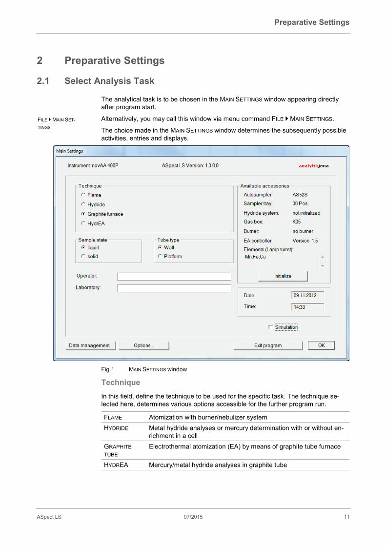
2 Preparative Settings
2.1 Select Analysis Task The analytical task is to be chosen in the MAIN SETTINGS window appearing directly after program start.
Alternatively, you may call this window via menu command FILE MAIN SETTINGS.
The choice made in the MAIN SETTINGS window determines the subsequently possible activities, entries and displays.
Fig.1 MAIN SETTINGS window
Technique In this field, define the technique to be used for the specific task. The technique se-lected here, determines various options accessible for the further program run.
FLAME Atomization with burner/nebulizer system HYDRIDE Metal hydride analyses or mercury determination with or without en-
richment in a cell GRAPHITE TUBE
Electrothermal atomization (EA) by means of graphite tube furnace
HYDREA Mercury/metal hydride analyses in graphite tube
FILE MAIN SET-
TINGS
Preparative Settings
12 07/2015 ASpect LS
Sample state and tube type Only for graphite tube technique and HydrEAtechnique
LIQUID Samples are available in liquid (dissolved) state. For atomization, a tube type must be selected in addition: WALL Uses a graphite tube without platform. Atomization of sample
matter occurs at the wall of the graphite tube. PLATFORM Uses a graphite tube with platform. Atomization takes places on
the platform. Selections for tube type will have an influence on the depth to which the dosing tube of the micro pipetting unit will dip in the tube.
Only for graphite tube technique
SOLID Samples are available in solid state (powder, etc.). Sample matter is atomized in a special graphite tube for solid analytics. A sample can be placed in the graphite tube furnace using the automatic SSA600 autosampler or the manual SSA6 sampler.
Appliance Configuration Before starting a measurement the appliance and PC must be connected. Verify that the spectrometer and the accessory to be used are connected and ready for opera-tion. The button [INITIALIZE] triggers the recognition and configuration of spectrometer and accessories depending on the technique selection and the recognition of the hol-low cathode lamps (HCL) and super hollow cathode lamps (SHCL) available in the lamp turret (only for AAS appliances with coding unit).
On exiting the MAIN SETTINGS window with the [OK] button, the system checks the state of initialization and informs the operator of the necessity of initialization, if neces-sary.
Detected accessory units are listed by name. If an accessory is identified as NOT INI-TIALIZED, its initialization was skipped because of the technique selected (e.g. the hy-dride system if the flame technique has been selected); if --- is displayed, the respec-tive accessory was not detected.
In the DATE and TIME field, the current system time of the PC is displayed.
If you use the optionally installable user management, the OPERATOR input field shows the registered user. If you do not use user privilege management, you may enter the operator’s name manually (30 characters).
In the LABORATORY field, you can type in a name of up to 30 characters. The name entered last is saved and issued as information on result reports.
For trainings and demonstration purposes, you may operate ASpect LS without an AAS device being connected. To this end, activate the SIMULATION checkbox. Then, all device functions (including data acquisition and analysis) will be run in simulation mode.
Preparative Settings
ASpect LS 07/2015 13
2.2 Lamp turret, mounting
Call up the window SPECTROMETER or the symbol and change to the tab CONTROL.
Use [LAMP TURRET] to open the window of that name
The window LAMP TURRET shows the current stocking of the 6 lamp or 8 lamp turret. For appliances with a lamp coding unit the stocking of the lamp turret for lamps with RFID Chip is established automatically on initialization of ASpect LS.
For appliances with 8 lamp turret super hollow cathode lamps (S-HCL) can be used on the places 5 to 8. For appliances with a 6 lamp turret only lamp position 6 can be stocked with an S-HCL if it is equipped with the necessary power supply.
Fig.2 LAMP TURRET window
Table area
POS Position of the hollow cathode lamp in the lamp turret TYPE Lamp type COD. Only appliances with coding unit
If a coded lamp is stocked on the lamp position, then the entry receives a star ("*"). The lamp parameters are established auto-matically in this case and they cannot be changed manually.
ELEMENTS The elements to be analyzed with this lamp MAX. CURRENT Maximum possible lamp current MAX. BOOST. Maximum possible boost current for S-HCL RECOMMENDED CURRENT
Recommended lamp current for coded lamps
RECOMMENDED BOOST.
Recommended boost current with coded S-HCL
CONTROL TAB

Preparative Settings
14 07/2015 ASpect LS
ADJ. If marked with "*", the lamp was adjusted (→ "Adjusting The Lamps" below).
JUST. VALUE Adjusted value of the lamp, is required for customer service. Control buttons
[CHANGE] Change the parameters for the marked lamp position. The window "Select Lamp/Element" appears. NOTE FOR CODED LAMPS: The lamp parameters of coded lamps are established automatically and cannot be changed.
[REGISTER LAMP]
Only appliances with coding unit Identify the lamp with the selected lamp position. For coded lamps the parameters are established and entered.
[DEREGISTER LAMP]
Delete all lamp parameters of the selected line.
[INITIALIZE] Move the lamp turret into the basic state. On initializing the lamp information is transferred to the program.
[DELETE TABLE] Delete all positions without confirmation requests. [CHANGE LAMP] Switch off the selected lamp and drive the lamp turret to the lamp
change position. The lamp then can be changed after a sufficient cooling.
Lamp Adjustment For lamps the optical axis can differ from the mechanical axis. In the result the possi-ble energy maximum does not come to the recipient. During the automatic adjustment the lamp turret is turned until the energy maximum is reached. Newly fitted lamps should thus always be adjusted.
The adjustment of HCL and SHCL occurs automatically following activation of the button [ADJUST]. The adjustment value is permanently stored and the lamp is marked with "*" in the column ADJ.. The adjustment must only be repeated on replacing the lamp.
Following changing of a D2-HCL this must also be adjusted in accordance with energy maximum. The adjustment occurs in the window SPECTROMETER ( → "Adjust D2-HCL" pg. 99).
Caution! Place uncoded lamps in specified positions!
Note for appliances without lamp coding unit (novAA 400): The lamps are not coded, there is no feedback between the lamp turret and the PC. In order to avoid measure-ment errors it is imperative that you mount the lamps according to their entered posi-tions.
Preparative Settings
ASpect LS 07/2015 15
2.3 Specify uncoded lamps Specify the uncoded lamps in the lamp turret in the window SELECT LAMPS/ELEMENT.
Call up the window SPECTROMETER with the symbol and change to the tab CONTROL.
Use [LAMP TURRET] to open the window of that name
Mark the position of the lamp turret in the table which you stock with a lamp or the stocking of which you wish to change.
Open the window SELECT LAMP/ELEMENT with [CHANGE].
Fig. 3 SELECT LAMP/ELEMENT window
Enter the following values:
LAMP PO-SITION
Display position in the lamp turret. Cannot be edited in this window.
LAMP TYPE Selection of the lamp type. This selection is focused on the lamp posi-tion and the lamp types which are possible there. S-HCL and S-MHCL are only available on the positions 5 to 8 for the 8 lamp turret and only on position 6 for the 6 lamp turret. NONE position contains no lamp. HCL Single-element hollow cathode lamp M-HCL (multi-element hollow cathode lamp) S-HCL Super hollow cathode lamp with one element S-MHCL Super hollow cathode lamp with several elements
CURRENT Set maximum lamp current. BOOST Only with S-HCL and S-MHCL
Set maximum boost current.
CONTROL TAB
Preparative Settings
16 07/2015 ASpect LS
PERIODIC TABLE
Select lamp element in the periodic table with a mouse click on the el-ement symbol: Blue buttons identify selectable elements. Grey (inactive) buttons mark elements which cannot be analyzed with AAS technology. Green ele-ment buttons define selected elements. For M-HCL and S-MHCL several elements can be clicked. A further click on an element symbol cancels the selection. Selected elements are displayed in the table to the side.
Select the window LAMP/ELEMENT with [OK] and return to the lamp turret window.
The lamp specification is entered into the table of the window Lamp Turret.
Methods
ASpect LS 07/2015 17
3 Methods
3.1 Manage Methods
3.1.1 Create new method To create a new method, activate menu command FILE NEW METHOD. A selec-
tion dialog with the following options opens.
BASED ON DEFAULT PARAMETERS
Opens a window for the entry of new method parameters (only with editable default settings for calibration and sta-tistics).
BASED ON CURRENT PARAMETERS
Open the METHOD window with the currently set method parameters.
BASED ON SAVED METHOD…
Activate the LOAD METHOD dialog. After the selection of the method, its parameters are dis-played in the METHOD window.
Choose the desired option and open the METHOD window.
Alternatively, activate the METHOD window by a click on the button or by menu command METHOD DEVELOPMENT METHOD. This will bring up the Method window with the currently set method parameters.
The functions of labeled and icon buttons in the METHOD window are described in section "Frequently used control elements" pg. 8.
Activate the selected method parameters with the [OK] or the [ACCEPT] button for the following analysis.
3.1.2 Save methods Methods are managed in the database window (→"The database window" pg. 168).
The command for saving the current method parameters can be given in different ways.
In the METHOD window, click on the [SAVE] button.
Alternatively, you may activate menu command FILE SAVE METHOD.
This will bring up the SAVE METHOD window.
In the NAME textbox, type the desired method name.
In the field CAT.: (category), you may optionally enter an additional identifier of maximally three characters to facilitate later sequence search in the database.
In the DESCRIPTION field, you can optionally enter information on the method.
Save the method with [OK].
On doing so, the method will be saved to the database. If you choose an existing method name, the existing method will not be overwritten, but a new version created in the database. To remove methods from the database, you must explicitly delete them!
FILE NEW METHOD
METHOD DEVELOP-
MENT / METHOD...
FILE SAVE
METHOD

Methods
18 07/2015 ASpect LS
Note
The method is also saved in the result file of the measurement. After having opened the results file, you may also reproduce the method.
3.1.3 Opening methods Activate menu command FILE OPEN METHOD... or, on the toolbar, click on the
folder symbol right of the METHOD field.
Alternatively, you may click on the [OPEN] button in the Method window.
This will bring up the LOAD METHOD window.
Choose the desired method from the list.
By the entry in the CAT textbox, you can define that only methods of the specified category are displayed. If you want to see methods of all categories, delete the entry in the CAT field.
Activate the CURRENT VERSION ONLY check box, if with methods of the same name you want to see the method of the highest version number only.
Open the selected method with [OK].
3.2 Specify Methods
3.2.1 Select analyses lines - LINES tab The element lines are to be specified in the METHOD / LINES window. You may choose a maximum of 200 different lines.
Fig. 4 Window METHOD / LINES with selected element lines
FILE OPEN METH-
OD...
LINES TAB

Methods
ASpect LS 07/2015 19
The following line parameters must be defined:
NO. Number of element line ELEM. Element symbol (up to 2 characters) WAVEL. [NM]
Wavelength of analysis line in nm After click on this table cell another analysis line of the same element can be selected in a list.
LINE Designation of analysis line You can choose a free name, which serves to clearly identify the analy-sis line (10 characters).
OPT. BA Optical working mode for flame and hydride technique: SINGLE BEAM
The light is directed through the sample chamber, the lamp drift is corrected by an automatic autozero directly before measurement.
DOUBLE BEAM In the measurement of the reference signal the light on the sample chamber is guided past and used for correction of the lamp drift.
EMISSION Measurement of the emission signal of the element in the flame
LAMP Lamp type used: HCL Single element hollow cathode lamp S-HCL Super hollow cathode lamp with one element MHCL Multielement hollow cathode lamp S-MHCL Super hollow cathode lamp with several elements
CURRENT Set lamp current (not for the working mode Emission) BOOST Set boost current (only for S-HCL) SLIT Set slit width
With the button [APPEND] and [INSERT] you add a new analysis line to the end of the list or before the selected line. With [DELETE] you remove a marked line from the list.
Insert element lines into the list In the METHOD / LINES window, click on [APPEND] to open the window SELECT EL-
EMENT/LINE.
Methods
20 07/2015 ASpect LS
Fig. 5 SELECT ELEMENT/LINE window
The selection dialog contains a periodic chart and a line table. In the periodic chart the selectable elements are depicted as blue buttons. Elements for which a lamp is pre-sent in the lamp turret are marked in bold. The line table contains the following col-umns:
ELEMENT Element symbol LINE Wavelength in nm TYPE P = Primary line, S = Secondary line, * = own line SENSITIVITY Analysis sensitivity of the line. The sensitivity of the primary line is
equivalent to 100%. By activating the ELEMENT or the LINE option button, the line table is sorted in-
creasingly by either the chemical symbol or the wavelength.
If you click on an ELEMENT SYMBOL in the periodic system (blue buttons are se-lectable elements), the lines of the selected element will be displayed in the line table. Alternatively, you may enter the element symbol in the SELECT ELEMENT text box. To have the complete element list displayed again, delete the entry in the SELECT ELEMENT text box.
To select the analysis lines to be used, successively click on the corresponding rows in the line table. The selected analysis lines appear under the periodic system.
To undo the selection of a line, click on it once more in the line table. With the [DESELECT] button, you can deselect all lines previously selected.
Confirm your choice of analysis elements/lines with [OK].
As a pre-setting for further method processing the parameters from either the COOKBOOKor the METHOD DATABASE can be taken over in the list field DEFAULT-PARAMETERS OF (→ "Cookbook" pg. 161).
The selected elements/lines are taken into the table in the METHOD - LINES window.

Methods
ASpect LS 07/2015 21
NOTE
You can select several lines with varying sensitivity for an element.
3.2.2 Specify evaluation parameters - EVALUATION tab On the tab EVALUATION specify the type and form of the signal evaluation.
Fig. 6 METHOD / EVALUATION window (Example for flame technique)
The following line parameters must be defined:
NO. Number of element line ELEM. Element symbol LINE Line designation INT.MOCE MEAN Absorbance (emission) averaging over the emission
time. AREA Calculation of the peak area of the absorbance (emis-
sion) over the integration time. HEIGHT Calculation of the peak height (largest value after
smoothing) of the absorbance (emission) during the inte-gration time.
BACKGROUND NO BACKGROUND No background correction, deuterium-HCL switched off.
D2HCL-BACKGROUND Measurement of the background radiation for elimination of the non-specific absorption, deuterium-HCL switched on.
ONLY D2HCL-BACKGROUND Only background measurement, but no sample meas-urement. Deuterium-HCL switched on.
EVALUATION TAB
Methods
22 07/2015 ASpect LS
The special background corrections for the ZEEman-AAS are de-scribed in the section below.
EMS-WD (NM)
Only for flame-emission measurements with the integration types MEAN VALUE and RUNNING MEAN VALUE Wavelength difference (in nm) to analysis line, with which the emis-sion background is measured. In order to be able to measure samples with a high emission back-ground (e.g. salts), there is the possibility of detecting the back-ground next to the analysis line and subtracting it from the measured emissions.
SMOOTHING Smoothing of the measurement value peak AZDK AZ-drift control. When switched on, during the autozero phase (AZ)
of the furnace program a testing of the energy fluctuation of the lamp occurs.
Note! Advice on the selection of the "Int. mode"
MEAN (VALUE): To be used for sufficiently high sample volumes available (flame tech-nique; seldom: hydride technique).
AREA AND HEIGHT: For the atomization of a defined sample volume (graphite tube tech-nique, hydride technique or, in combination with an injection module, in flame technique).
Background corrections special for ZEEman-AAS (graphite tube furnace and HydrEA-technique)
NO BACK-GROUND
No background correction, deuterium-HCL or Zeeman magnet is off.
ZEEMAN-2-FIELD MODE
Background correction by means of Zeeman-2-field-mode, Zeeman magnet on. In the column MAX. FS [T] set the maximum field strength in Tesla.
ZEEMAN-3-FIELD MODE
Background correction by means of Zeeman-3-field-mode, Zeeman magnet on. In the column MAX. FS [T] set the maximum field strength and in MED. FS [T] set the mean field strength in Tesla.
ZEEMAN DYN. MODE
Background by means of Zeeman-dynamic-mode, Zeeman magnet on. In the column MAX. FS [T] set the maximum field strength and in MED. FS [T] set the mean field strength in Tesla. In the column LIMIT STD.NO. enter the number of the standard with the limit concentra-tion.
ONLY ZEEMAN-BACKGR.
Only background measurement. No sample measurement. Zeeman magnet on.
D2-BACKGROUND
Measurement of the background radiation for elimination of the non-specific absorption by means of deuterium-HCL. Deuterium-HCL on, Zeeman-Magnet off.

Methods
ASpect LS 07/2015 23
Note
For the 2-field and 3-field modes of the Zeeman-background correction an automatic optimization program can be started (→ "Optimize ZEEman magnetic field" pg. 103). The special features of the Zeeman-dynamic-mode are explained in the section "The ZEEman dynamic mode" pg. 104.
3.2.3 Specify flame parameters - FLAME tab Selected technique Flame technique Burner parameters and gas flows for flame technique are adjusted in the METHOD - FLAME window.
Fig.7 METHOD - FLAME window with burner and gas flow settings
Line-independent settings for the burner/nebulizer system (BNS) First, adjust those parameters that apply to the complete method and that cannot be varied for the analysis of individual elements/lines.
Flame
SCRAPER The scraper is activated for the automatic analysis process with the 50-mm burner and acetylene/nitrous oxide flame. Now and then, the burner head is automatically cleaned by the scraper. Cleaning can be per-formed BEFORE EACH SAMPLE, BEFORE EACH 3RD MEASUREMENT, BEFORE EACH 2ND MEASUREMENT or BEFORE EACH MEASUREMENT.
OXIDANT (AUX.)
OFF: Operation without auxiliary oxidant ON: Operation with auxiliary oxidant
FLAME TAB

Methods
24 07/2015 ASpect LS
Note
When working with auxiliary oxidant, optimize the flame parameters manually (→ "Manual flame optimization", pg. 108).
Burner/nebulizer
TYPE Selection of the used type of burner: 50 MM or 100 MM BURNER ANGLE [DEG]:
Angular position of the burner relative to the optical axis The burner angle must be set manually on the burner (normally it is set to 0°). The entry of the value is optional. It only serves to complete analysis method and report data. Value range: 0 –90°
NEBULIZER RATE [ML/MIN]
Aspiration rate of the nebulizer The aspiration rate is a nebulizer-specific value. The entry of the value is optional. It only serves to complete analysis method and record data. Value range: 1.0 – 9.9 ml/min
Line-dependent parameters for gas flow and burner height The parameters flame type, fuel gas flows and burner heights are dependent on the element and analysis line. If they are known for the elements to be analyzed, they can be entered directly into the table.
For the use of auxiliary oxidant, the following fuel gas flows are possible:
Auxiliary Oxidant Gas flows Air 75 / 150 / 225 NL/h Nitrous oxide (N2O) 60 / 120 / 180 NL/h
The use of the auxiliary oxidant is useful if combustible liquids shall be analyzed, a higher oxidant flow is necessary, or the fuel rate shall be increased.
The values can however be established manually or automatically in the program for flame optimization and transferred into the table (→ "Optimizing the flame" pg. 108).

Methods
ASpect LS 07/2015 25
3.2.4 Enter furnace program - FURNACE tab Selected technique Graphite tube technique, HydrEA tech-nique METHOD FURNACE is the window that provides a survey of essential parameter settings for furnace programs to atomize the various elements being analyzed.
Fig. 8 METHOD / FURNACE window with furnace parameter settings
To serve as default settings for atomization of the various elements using graphite tube technique, the respective furnace program data from the cookbook are preset. The furnace program can be edited for any analytical line in the FURNACE window and transferred into the current method (→ "Editing a furnace program" pg. 112).
The related list includes the following furnace program parameter items:
LINE Name of element line TOT. Total number of furnace program steps DRY. Number of drying steps in a furnace program PYROL. TEMP.
Pyrolysis temperature in °C
ATOMIZE Detailed display of temperature data during atomization phase: TEMP. End temperature of atomization phase RAMP Temperature variance during atomization phase in °C/s GAS Feeds inert gas
INJ. NO MARK Sample is injected before start of furnace program "*" Sample is injected at some later point in time
PRETR. Thermal preparation Sample and modifiers will be thermally prepared if this item was marked.
ENR. Enriches the sample if marked
FURNACE TAB

Methods
26 07/2015 ASpect LS
MODIFIER Additionally involved modifiers. For each measurement, a maximum of five additional modifiers can be selected.
Control buttons
[EDIT FURNACE PROGRAM]
Opens the FURNACE – FURNACE PROGRAM window that provides a full display of the furnace program. Furnace parameter settings can be adapted for any element line subject to analysis (→ "Editing a furnace program" pg. 112). Alternatively you can also open the window FURNACE - FURNACE PROGRAM with a double click on the line of the analysis line.
[ACCEPT FUR-NACE PRO-GRAM]
Validates the parameter settings of a marked analytical line for all subsequent lines in the list.
[MODIF. EX-TRAS...]
Opens the Furnace – Modif.+Extras window for specifying matrix modifiers (→ "Matrix modifiers, selections for enrichment and pre-treatment" p. 115)
"CLEAN FURNACE" as an additional sequence action The furnace will be cleaned by baking out on completion of a furnace program for a given element line in all cases. In addition, a further cleaning step can be defined for a particular sequence by selecting CLEAN FURNACE (→ "Combine sample and action sequences for a sequence" pg. 59). The parameters for this action can be entered in the ACTION CLEAN FURNACE subarea.
TEMP.[°C] Specified end temperature for baking (cleaning) process. RAMP [°C/S] Rate of temperature change HOLD [S] Holding time at end temperature
Methods
ASpect LS 07/2015 27
3.2.5 Specify Hydride and HydrEA systems- HYDRIDE tab Selected technique Hydride/HydrEA technique
Fig. 9 METHOD / HYDRIDE window
The hydride system parameters for HS 60 A/HS 60, HS 55 A/HS 55, HS 60 modular and HS 55 modular are to be adjusted in the METHOD / HYDRIDE window. The hydride system connected is detected during device initialization.
The parameters for the hydride injector HS50 are defined in the SAMPLE TRANSPORT tab (→ "Auto sampler for flame and hydride/HydrEA technique" pg. 31).
Note
The commands for additional washing or loading of the hydride system are released from the HYDRIDE SYSTEM window (→ "Hydride system" pg. 124).
Mode You can choose among different modes depending on the equipment of the hydride system.
HYDRIDE (CON-TINUOUS)
Operation with autosampler or manual. The reaction takes place in the reactor under continuous conditions (HS 60 A/HS 60/HS 60 modular).
HYDRIDE (BATCH)
Manual mode. The sample is pipetted into the reaction beaker (max. 30 mL). The beaker is to be clamped gas-tight to the head of the batch module. With the first channel of the 4-channel peristaltic pump, the reduct-ant is pumped into the reaction beaker. The fast and partly vigor-ous reaction liberates metal hydride or atomic Hg vapor (HS 55 A/HS 55/HS 55 modular).
HYDRIDE TAB

Methods
28 07/2015 ASpect LS
FBR MODE Only for hydride technique in continuous operation (Fast Baseline Return, FBR) After the maximum absorption has been reached, the direct argon gas flow purges the cell free during WASH TIME 2 (Wash 2) thus causing a fast return of the signal to baseline level.
Cell temperature / Pump speed level
CELL TEMP.[°C]
Only for hydride technique For the hydride formers As, Se, Sn, Sb, Te and Bi, the cell tempera-ture is selectable in the range between 600°C and 1000°C. For Hg analyses, you may choose between RT (room temperature < 60°C) or 150°C. THE CELL IS HEATED TO THE SELECTED CELL TEMPERATURE AT THE START OF THE ANALYSIS PROCESS, OR YOU MAY START IT IN THE HYDRIDE SYSTEM WINDOW.
PUMP SPEED LEV-EL
Four speed levels (1 - 4) are available for the transport of the sample (in continuous mode) and the components. In continuous mode, the supplied sample volume is determined on the basis of the pump speed level selected and the reaction time.
System cleaning For continuous operation
System cleaning may be selected optionally after every sample measurement and/or arranged as an action.
BETWEEN SAMPLES
System cleaning after each sample measurement OFFSystem is not cleaned. CLEANING WITH ACID System is rinsed after every sample with dilut-
ed acid. The corresponding time is to be defined under WASH TIME ACID. When half of the wash time is over, the sample path is switched to the reactor.
CLEANING WITH REDUCTANT + ACID This cleaning method is the method of choice if the system is heavily contaminated (samples with high element contents). First, the system is rinsed with reductant for the selected WASH TIME REDUCT-ANT. This process is followed by a wait time (SOAK TIME) to allow the reductant to take effect onto the deposits on the tube walls. Finally, the system is rinsed with diluted acid for the WASH TIME ACID.
AT ACTION The system cleaning can be set as a programmable special action (→ "Combine sample and action sequences for a sequence" S 59). This additional cleaning step can be inserted after samples with high ana-lyte content. CLEANING WITH ACID see option BETWEEN SAMPLES CLEANING WITH REDUCTANT + ACID see option BETWEEN SAMPLES
POS. RE-DUCTANT
Position of reductant on the sample tray.
[WASH TIMES]
A window is opened for the definition of three wash times: WASH TIME REDUCTANT, SOAK TIME, WASH TIME ACID. Please set these values according to the selected cleaning options.

Methods
ASpect LS 07/2015 29
Operation times The operation times are to be adjusted dependent on the selected operating mode. All operation times are entered in seconds.
SAMPLE LOAD TIME
Time in which the sample pump loads the sample tube up to the two-valve assembly with sample. This time is needed only for the first measurement of a new sample.
AZ WAIT TIME Time directly preceding the baseline (auto zero) adjustment. PREWASH TIME
Time for purging the beaker with argon before the reaction (for hy-dride formers). The prewash time is used to purge off air in order to prevent an oxy-hydrogen reaction in the following reaction.
REACTION TIME
Time in which the sample pump pumps sample into the reactor. This is the crucial parameter for the supplied sample volume and the measuring sensitivity.
PUMP TIME Time in which reductant is pumped into the beaker in order to start a reaction.
WASH TIMES 1-3
Times used to convey the reaction gas by means of the argon flow. The transport paths are different in the individual phases for the vari-ous operating modes. The transport paths can be presented graphically.
HEAT. TIME COLLECTOR
Time in which the collector heating is on in order to release the en-riched Hg.
COOL. TIME COLLECTOR
Time in which the collector is ventilated in order to cool it down for a new enrichment cycle.
GAS FLOWS Defines the argon flow flowing in the phases displayed left of it. The adjusted gas flow applies until a new gas flow can be entered. The gas flow can be switched over with varying frequency for the different operating modes. The gas paths for the individual phases are illus-trated in the graphic of the analysis process on the hydride system (→ "Present gas flows and analysis procedures of the hy-dride/HydrEA system graphically", pg. 30). The gas flows are adjust-able in three steps from 5 to 15 Liters/hour.
Batch Parameters
SAMPLE VOLUMES Here, enter the volumes of the sample in the beaker. ENRICHMENT CY-CLES
For the batch operation with Hg enrichment on the collector Define the number of beakers, the content of which is en-riched.
[Plot] button By a click on the [PLOT] button, you can open the graphic presentation of the gas paths for the individual phases of the analysis process.
Methods
30 07/2015 ASpect LS
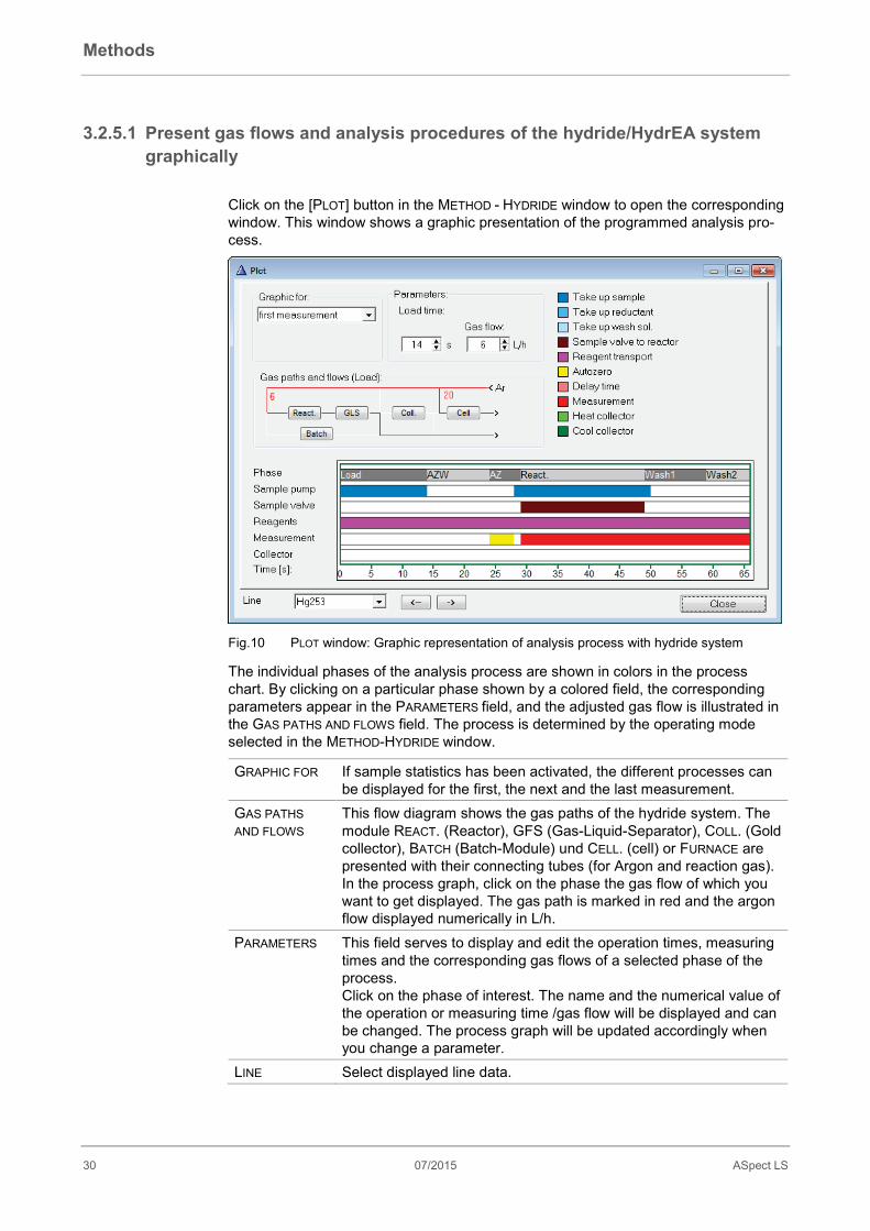
3.2.5.1 Present gas flows and analysis procedures of the hydride/HydrEA system graphically
Click on the [PLOT] button in the METHOD - HYDRIDE window to open the corresponding window. This window shows a graphic presentation of the programmed analysis pro-cess.
Fig.10 PLOT window: Graphic representation of analysis process with hydride system
The individual phases of the analysis process are shown in colors in the process chart. By clicking on a particular phase shown by a colored field, the corresponding parameters appear in the PARAMETERS field, and the adjusted gas flow is illustrated in the GAS PATHS AND FLOWS field. The process is determined by the operating mode selected in the METHOD-HYDRIDE window.
GRAPHIC FOR If sample statistics has been activated, the different processes can be displayed for the first, the next and the last measurement.
GAS PATHS AND FLOWS
This flow diagram shows the gas paths of the hydride system. The module REACT. (Reactor), GFS (Gas-Liquid-Separator), COLL. (Gold collector), BATCH (Batch-Module) und CELL. (cell) or FURNACE are presented with their connecting tubes (for Argon and reaction gas). In the process graph, click on the phase the gas flow of which you want to get displayed. The gas path is marked in red and the argon flow displayed numerically in L/h.
PARAMETERS This field serves to display and edit the operation times, measuring times and the corresponding gas flows of a selected phase of the process. Click on the phase of interest. The name and the numerical value of the operation or measuring time /gas flow will be displayed and can be changed. The process graph will be updated accordingly when you change a parameter.
LINE Select displayed line data.
Methods
ASpect LS 07/2015 31
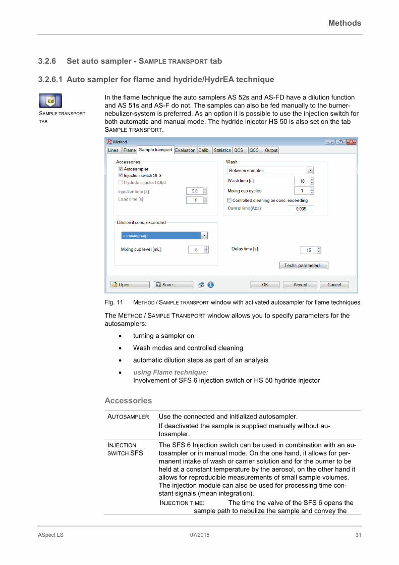
3.2.6 Set auto sampler - SAMPLE TRANSPORT tab
3.2.6.1 Auto sampler for flame and hydride/HydrEA technique In the flame technique the auto samplers AS 52s and AS-FD have a dilution function and AS 51s and AS-F do not. The samples can also be fed manually to the burner-nebulizer-system is preferred. As an option it is possible to use the injection switch for both automatic and manual mode. The hydride injector HS 50 is also set on the tab SAMPLE TRANSPORT.
Fig. 11 METHOD / SAMPLE TRANSPORT window with activated autosampler for flame techniques
The METHOD / SAMPLE TRANSPORT window allows you to specify parameters for the autosamplers:
• turning a sampler on
• Wash modes and controlled cleaning
• automatic dilution steps as part of an analysis
• using Flame technique: Involvement of SFS 6 injection switch or HS 50 hydride injector
Accessories
AUTOSAMPLER Use the connected and initialized autosampler. If deactivated the sample is supplied manually without au-tosampler.
INJECTION SWITCH SFS
The SFS 6 Injection switch can be used in combination with an au-tosampler or in manual mode. On the one hand, it allows for per-manent intake of wash or carrier solution and for the burner to be held at a constant temperature by the aerosol, on the other hand it allows for reproducible measurements of small sample volumes. The injection module can also be used for processing time con-stant signals (mean integration). INJECTION TIME: The time the valve of the SFS 6 opens the
sample path to nebulize the sample and convey the
SAMPLE TRANSPORT
TAB
Methods
32 07/2015 ASpect LS
aerosol to the burner. The time depends on the highest concentration to be expected. Typical values: 0.5 ... 2.0 s.
LOAD TIME: The time needed to fill the sample aspiration path be-tween sample cup and injection module with new sam-ple.
DIP TECHNIQUE As an alternative to the injection switch, small sample volumes may result by briefly dipping the aspirating canula into the sample. The advantage is a smaller dead volume than with the injection switch. The dip technique will be activated once the signal evalua-tion is set to peak area or peak height and the injection switch is deactivated. For using this technique a possibly installed SFS 6 has to be removed from the tubing. DIP TIME: The time the aspirating canula should be dipped into
the sample cup. MEAS START DELAY: The time from the beginning of the sample
aspiration until reaching the flame. Note: Because of continuously sample transport each sample tube (standards and samples) has to contain the equal sample volume.
HYDRIDE INJEC-TOR HS50
The hydride injector HS 50 is a purely pneumatic batch system for manual operation. It consists of batch installation and cell holder with quartz cell. The reductionagent solution is transported pneu-matically from the supply bottle into the reaction tank. The quartz cell is heated by the flame. The operation times of HS50 are con-trolled by the AAS software in a simple way. Peak area mode as well as peak height mode is possible. The measurement procedure is divided in following parts: Prewash – Autozero – Reaction/Integration. REACTION TIME
Set reaction time. During the reaction phase reaction agent is transferred to the reaction beaker. The measurement signal acqui-sition starts simultaneously. The integration time has to be set in a way to acquire the total signal.
Prewash time Set prewash time. During the prewash time the reaction beaker is flushed free from air. The prewash phase is omitted for the de-termination of Hg because the argon flow is necessary in order to transport the Hg out of the sample.
SAMPLE VOLUME Define sample volume.
DELAY TIME Time which is needed to transport the sample to the atomization unit (e.g flame or reaction chamber in the hydride system). The time is essentially determined by the length of the sample tubes. This time is needed to convey the sample to the flame.
Use autosampler for automatic dilution Samples may be diluted automatically for autosamplers with integrated dilution func-tion.
Methods
ASpect LS 07/2015 33
General dilution parameters are defined in the method (DILUTION MODE and MIXING CUP LEVEL). Individual dilution factors for each sample may be entered in window SAMPLE ID (→ "Specify information data for samples and QC samples" pg. 65).
In addition you can choose the parameter for an automatic DILUTION IF CONCENTRATION EXCEEDED. If the value for concentration is found to exceed the measuring range as determined by the respective calibration graph by more than 10 %, the sample will be diluted.
The dilution is performed in the mixing cup. Required volumes are mathematically determined as part of a program sequence, depending on the extinction value for un-diluted solution state. Once calculated, the analyte volume is introduced into the mix-ing cup and the mixing cup is then filled with diluent solution to the predefined fill level. The amount of diluent solution is drawn from the storage bottle for diluent solution.
Parameters for Dilution
DILUTION IF CONC. EXCEED
NONE Samples are not automatically diluted if the concen-tration is above the calibration range.
IN MIXING CUP Samples are are automatically diluted if the concen-tration is above the calibration range as described above.
MIXING CUP LEVEL [ML]
The fill level to which the mixing cup will be filled up with diluent solution.
Specify washing steps While a measurement sequence is running, you can specify washing steps to clean the various sample paths inside the system and its accessory units.
WASH MODE OFF Wash mode switched off. No rinsing performed automati-cally.
BETWEEN SAMPLES Washes after each sample, but not within a statistical series.
WASH TIME Time in which the rinsing agent is aspirated in the wash cup. Includes washing of tube path and burner-nebulizer system.
MIXING CUP CYCLES
Number of wash cycles for mixing cup. Fills mixing cup with wash liquid/diluent solution and drains it again in one cycle.
Controlled cleaning Where analyzed samples are of a kind that result in exceeding the calibration graph working range by more than 10 %, the graphite tube, the burner-nebulizer system (flame technique) or the hydride system may be washed as may be appropriate for the currently selected technique, in order to remove contamination from a preceding measurement. During the wash, the absorbance/emission is measured in order to check the cleaning results.
Automatic controlled cleaning should be performed following measurement of highly concentrated samples, notably, with DILUTION ON CONC. EXCEEDING mode active.
CONTROLLED CLEANING
Will automatically trigger controlled cleaning on exceeding speci-fied concentration level if active.
Methods
34 07/2015 ASpect LS
CONTROL LIMIT The value, to which the signal level must have returned during rinsing, before the diluted samples / samples of lower concentra-tion are analyzed.
Note
Controlled cleaning can also be defined as part of a sequence, independently of a concentration exceeded situation.
Note on wash procedure of AS 52s/AS 51s and AS-FD/AS-Fautosampler To perform washing of the sample aspiration path and the burner-nebulizer system, the autosampler arm dips the needle into the wash cup of the autosampler. A mem-brane pump delivers wash liquid from a storage bottle for the time the needle is sub-merged. Its pump rate is greater than the aspiration rate of the nebulizer or that of the hydride system, respectively. The complete sample path is cleaned (cannula, sample tube, sample injector SFS6 and the burner-nebulizer system). Surplus amounts of washing liquid will flow off into the waste bottle.
The mixing cup of AS 52s or AS-FD is cleaned by filling with wash liquid/diluent solu-tion and draining it again in one single cycle.
Parameters for dipping depth and dosing speed Specific parameters of the autosampler, however, such as immersion depth in the various cups and pipetter speed levels are to be selected in the separate AU-TOSAMPLER window (→section "Autosampler " pg. 128). The AUTOSAMPLER window on this tab can be opened by clicking [TECHN. PARAMETERS].
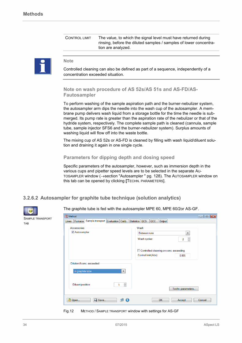
3.2.6.2 Autosampler for graphite tube technique (solution analytics) The graphite tube is fed with the autosampler MPE 60, MPE 60/2or AS-GF.
Fig.12 METHOD / SAMPLE TRANSPORT window with settings for AS-GF
SAMPLE TRANSPORT
TAB
Methods
ASpect LS 07/2015 35
The METHOD / SAMPLE TRANSPORT window allows you to specify parameters for these autosamplers:
• turning a sampler on
• Wash modes
• automatic dilution steps as part of an analysis
Use autosampler for automatic dilution In connection with the autosampler an automatic sample dilution can be carried out. Individualized dilution factors can be set for each sample in the SAMPLE-ID window. (→ "Specify information data for samples and QC samples" pg. 65). Method is availa-ble for general parameter settings (mode and position of the dilution agent) to achieve dilution.
When the concentration is more than 10% above the upper end of the calibration curve, automatic dilution of samples can be carried out as specified in parameter. The maximum dilution factor is limited by the smallest volume to be injected reliably (2µL).
A dilution in the mixing cup as described for AS 52 s/AS-FD is only possible with the MPE 60 (→ "Auto sampler for flame and hydride/HydrEA technique" pg. 31). For the MPE 60/2 and AS-GF an analyte reduction takes place directly in the graphite tube. In addition unused sample cups may be used for DILUTION WHEN CONCENTRATION IS EX-CEEDED.
DILUTION IF CONC. EXCEED
NONE Samples are not diluted. IN GRAPHITE TUBE:
The sample volume will be reduced in accordance with the dilution factor and placed into the graphite tube. The remaining balance against the initial sample volume will be replaced by diluent liquid.
REDUCED VOLUME: The sample volume will be reduced in accordance with the dilution factor and placed into the graphite tube. The remaining balance against the initial sample volume will not be replaced by diluent liquid.
IN MIXING CUP: MPE 60 only Dilution takes place in the mixing cup. The volume is al-ways filled up to 500 μl.
IN SAMPLE CUPS: AS-GF and MPE 60/2 only Samples are diluted in unused sample cups. The number of cups as well as the starting cup on the sample tray is specified by using NO. MIXING CUPS. Enter the filling vol-ume in field LEVEL IN MIX. POSITIONS. The positions of cups to be used for automatic dilution are reset for further use in window AUTOSAMPLER / TECHN. PARAMETERS with the button EMPTY MIXING CUPS (→ "Technical parameters of the autosampler MPE 60" pg. 140).
DILUTION IF CONC. EXCEEDED
Performs dilution as described above if active.
DILUENT PO-SITION
Selects position of diluent on the sample tray.

Methods
36 07/2015 ASpect LS
Specify washing steps While a measurement sequence is running, you can specify washing steps to clean the various sample paths inside the accessory units.
WASH MODE OFF Wash mode switched off. No rinsing performed automatically. BETWEEN MEASUREMENTS
Cleaning after each statistic run AFTER EACH COMPONENT
The autosampler is washed after transfer of each com-ponent into the graphite tube (modifier, standard, sample, etc.).
WASH CYC-LES
Number of wash cycles per wash, 1 to 5
MIXING CUP CYCLES
MPE 60 only Number of wash cycles for mixing cup. Fills mixing cup with wash liquid/diluent solution and drains it again in one cycle.
Controlled cleaning If samples are analyzed which result in the calibration graph working range being ex-ceeded by more than 10%, the graphite tube may cleaned by baking out in order to remove contamination from the previous measurement. During the cleaning, the ab-sorbance/emission is measured in order to check the cleaning results.
Automatic controlled cleaning should be performed following measurement of highly concentrated samples, notably, with DILUTION ON CONC. EXCEEDING mode active.
CONTROLLED CLEANING ON CONC. EXCEEDING
Will automatically trigger controlled cleaning on exceeding specified concentration level if active.
CONTROL LIMIT The value, to which the signal level must have returned during cleaning, before the diluted samples / samples of lower concentration are analyzed.
Note
Controlled cleaning can also be defined as part of a sequence, independently of a concentration exceeded situation.
Note on wash procedure for MPE 60 Following acceptance of the samples or other liquids the dosing tube is automatically cleaned with the cleaning liquid found in the storage bottle (deionized water, slightly acidified with 0.1 N HNO3). Here the cleaning liquid is pumped from the storage bottle through the dosing tube and into the wash cup of the autosampler.
Parameters for dipping depth and dosing speed Specific parameters of the autosampler, however, such as immersion depth in the various cups and pipetter speed levels are to be selected in the separate AU-TOSAMPLER window (→ "Technical parameters of the autosampler MPE 60" pg. 140). The AUTOSAMPLER window on this tab can be opened by clicking [TECHN. PARAME-TERS].
Methods
ASpect LS 07/2015 37
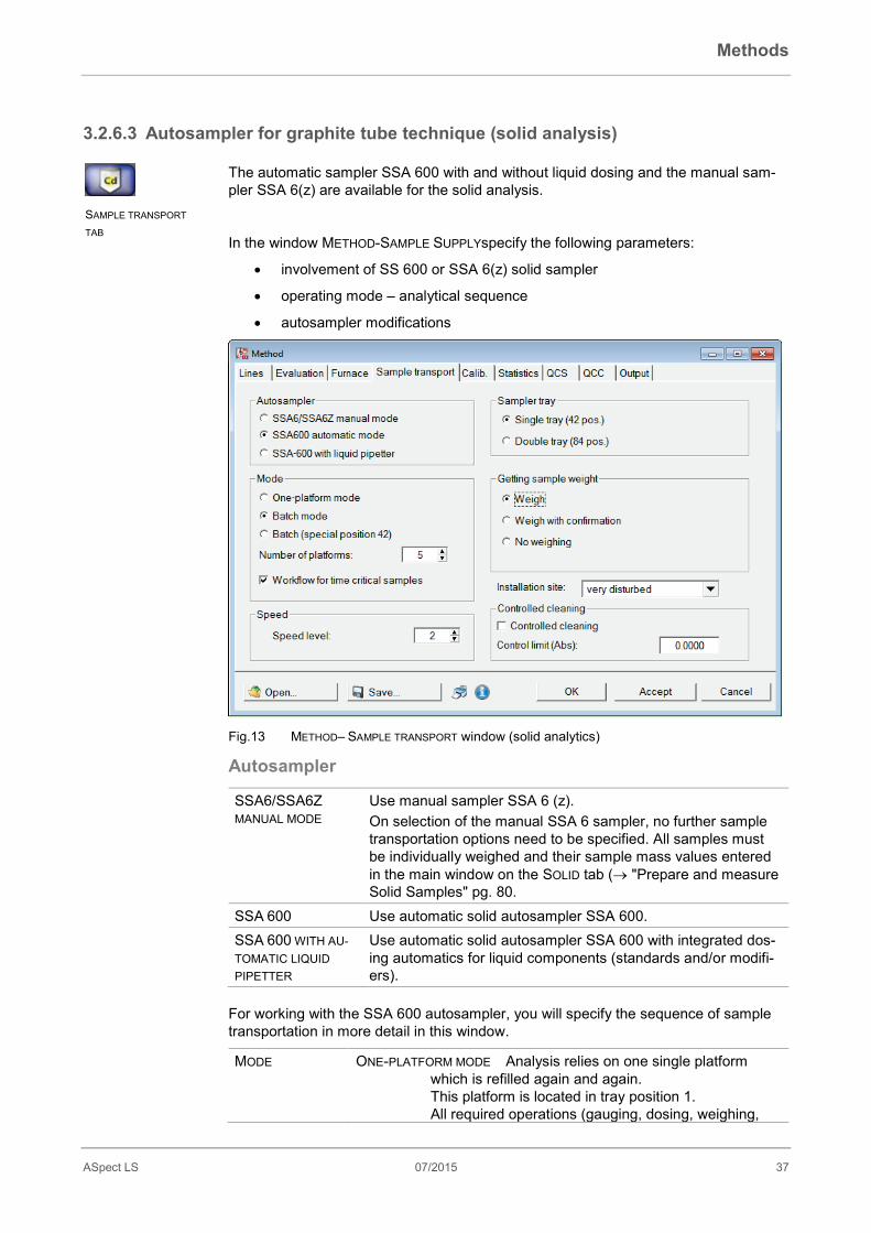
3.2.6.3 Autosampler for graphite tube technique (solid analysis) The automatic sampler SSA 600 with and without liquid dosing and the manual sam-pler SSA 6(z) are available for the solid analysis.
In the window METHOD-SAMPLE SUPPLYspecify the following parameters:
• involvement of SS 600 or SSA 6(z) solid sampler
• operating mode – analytical sequence
• autosampler modifications
Fig.13 METHOD– SAMPLE TRANSPORT window (solid analytics)
Autosampler
SSA6/SSA6Z MANUAL MODE
Use manual sampler SSA 6 (z). On selection of the manual SSA 6 sampler, no further sample transportation options need to be specified. All samples must be individually weighed and their sample mass values entered in the main window on the SOLID tab (→ "Prepare and measure Solid Samples" pg. 80.
SSA 600 Use automatic solid autosampler SSA 600. SSA 600 WITH AU-TOMATIC LIQUID PIPETTER
Use automatic solid autosampler SSA 600 with integrated dos-ing automatics for liquid components (standards and/or modifi-ers).
For working with the SSA 600 autosampler, you will specify the sequence of sample transportation in more detail in this window.
MODE ONE-PLATFORM MODE Analysis relies on one single platform which is refilled again and again. This platform is located in tray position 1. All required operations (gauging, dosing, weighing,
SAMPLE TRANSPORT
TAB
Methods
38 07/2015 ASpect LS
liquid dosing) are performed with this platform during an analytical process.
BATCH-OPERATION Analysis relies on several platforms. Anal-ysis may run automatically, depending on your pre-settings.
BATCH (SPECIAL POSITION 42) Analysis relies on several plat-forms. Analysis may run automatically, depending on your pre-settings. For samples requiring no weighing operation, for example, "Cal.Null" or liquid standards, position 42 on the sample tray will be used. For this reason, an empty platform must be placed in this posi-tion as pipetting destination of sample is necessary.
NUMBER OF PLATFORMS For BATCH-OPERATION and BATCH (SPECIAL POSITION 42) 42) Define the number of involved platforms and, hence, the number of available sample positions.
WORKFLOW FOR TIME CRITICAL SAMPLES
Controlling the behavior of the autosampler during the sample preparation and dosage. The samples are first mounted on the platforms directly before the measurement if active. This prevents the samples from volatizing during longer waiting periods on the sample tray or "creeping" across the platform due to high adhesion, as is the case with oils. This mode requires the constant presence of the user. All available platforms are prepared before the start of the meas-urement if disabled. All actions which require the presence of the user (sample feeding or manual pipetting of modifiers) are com-bined. The AAS device can measure in this mode without the constant presence of the user.
SPEED The speed of SSA 600 motion can be set in three stages. Recommended stage: 2
SAMPLER TRAY Number of trays placed one on top of the other. GETTING SAMPLE WEIGHT
WEIGH Once a dosed solid substance was weighed, the weighed portion value will be adopted without a pre-liminary query for acceptance of this weight.
WEIGH WITH CONFIRMATION Displays the result after each weighing. By pressing the green key (key at autosampler or [OK] in weighing window on the monitor screen), the user may signal his/her acceptance of the weighed portion result. On actuation of the orange key (key at autosampler or [REPEAT] in the weighing window on the monitor screen), the platform will return into dosing position, dosing will be altered and weighing will sub sequently repeat.
NO WEIGHING This weighing mode allows no measurement of con-centration. It is only intended for qualitative analysis of solid samples.
Methods
ASpect LS 07/2015 39
INSTALLATION SITE
Allows precision level settings for the integrated micro scales de-pending on the degree of interfering factors (especially excita-tion/vibration). If the time of weighing appears too long, it can be reduced by changing the setting for location site. This will be at the expense of precision. Available setting options are:
• very disturbed
• disturbed
• quiet
• very quiet
CONTROLLED CLEANING
Will automatically trigger controlled cleaning on exceeding speci-fied concentration level if active. If samples are analyzed which result in the calibration graph work-ing range being exceeded by more than 10%, the graphite tube and the sample platform are heated up in order to remove con-tamination from the previous measurement. The absorption is measured during the cleaning. The cleaning is ended if the control limit is reached. NOTE: Controlled cleaning can also be defined as part of a se-quence, independently of a concentration exceeded situation.
CONTROLL LIMIT (ABS)
Absorption to which the signal level must have returned during the cleaning before the next sample is measured.

Methods
40 07/2015 ASpect LS
3.2.7 Specify calibration parameters - CALIB.tab On the tab METHOD / CALIB.
• the selection of the calibration parameters occurs
• the specification of the making of the standards and their values
• the arrangement of the blank correction
For a calibration a maximum of 65 standards can be used.
Fig.14 METHOD– CALIB. WINDOW: Selection of calibration method and line-specific parameters
General calibration parameters Selection of calibration method
NO CALIBRATION The results of sample measurements are exclusively presented in absorbance or emission. Calibration is not necessary for these measurements. No fur-ther entries are required on the tab CALIB. The sequence list should, logically, only consist of samples.
STANDARD CALI-BRATION
Calibration is performed with samples of known concentration. The samples of unknown concentration are measured against these calibration standards.
WITH STANDARD ADDITION
Different quantities of a known sample are to be added to the unknown sample and the resulting substance measured. The concentration of the unknown sample results from the per-formed regression. The standard addition process is not available for solid analysis in a graphite tube.
METHOD OF ADDI-TIONS CAL-IB(RATION)
The calibration curve, by means of which other concentrations can be determined, is set up by the method of standard addi-tion. At the same time, the concentration of the first sample is found by this method.
CALIB.TAB
Methods
ASpect LS 07/2015 41
VARIABLE WEIGHTS/ADD.: For solid analysis / addition calibra-tion) Determine the number of different solid sam-ple weighed portions per addition series.
Standard preparation
MANUALLY The standard solutions are already prepared. PREP. BY SAMPLER
Only if AS52 s autosampler is included. The standard solutions are prepared in the mixing cup of the au-tosampler by mixing different portions of stock solution and diluent. In this case, adjust the following volumesfor preparing the standard solutions in the line table: MIX.VOL. Enter the total fill volume in the mixing cup (adjusting
range: 1 - 20mL). SAMPLE PART (only for addition method): The proportionate sample
volume (increments of 0.5 mL). With the addition method, the fraction of the sample solution of a measurement series is always the same. The proportionate sample solution must be smaller than the total fill volume. The difference vol-ume is filled up with stock solution and diluent solution. The sample volume/total volume ratio is the correction factor for the concentration to be computed.
BY VARIA-TION OF VOLUME
Only for graphite tube technique. Different volumes of stock solution or reference sample quantities are subjected to atomization in order to achieve a stepping in concentra-tion (referred to sample volume/sample weight).
BY DILUTION Only for graphite tube technique. Different volumes of stock solution and the amount of diluent solution required for achieving full sample volume are placed into the graphite tube in one transfer operation in order to achieve a stepping in con-centration (referred to the sample volume). In this case, adjust the following volumesfor preparing the standard solutions in the line table: VOL. [µL] The total volume to be brought into the graphite tube (1-50
µL). MAX.ADD.-VOL. (only for graphite tube technique / additionmethod)
Add maximum amount of stock solution. If the addition so-lutions were produced by dilution, this is the sum volume from the addition volume and the diluent volume.
Blank correction
Only for STANDARD-ADDITION METHOD and ADDITION-CALIBRATION.
ABSORBANCE COR-RECTED
In every standard addition procedure, the blank is measured too and the measured absorbance value subtracted from all measured values before the regression line is calculated. This method was customary for a long time; with many real samples however, it leads to incorrect results.
CONCENTRATIONS CORRECTED
First, a separate standard addition is carried out for the blank solution using the same concentration additions as for the sample. The found concentration will then be subtracted auto-matically from all other concentrations determined by standard addition.
Methods
42 07/2015 ASpect LS
Element specific calibration parameters in the table Volumes
Depending on atomization technique and calibration process various volumes must be defined (see above "Making of the standards").
Calibration function (only with Standard calibration)
LINEAR Calibration points result in linear calibration curve. The methods of standard addition and addition calibration are ap-proved only for linear calibration curves. 𝑦 = 𝑎𝑎 + 𝑏
NONLIN. RATIO. Calibration points result in a non-linear calibration curve of a ra-tional function. 𝑦 = 𝑎+𝑏𝑏
1+𝑐𝑏
NONLIN. QUADR,
Calibration points result in a non-linear calibration curve of a quad-ratic function. 𝑦 = 𝑎𝑎2 + 𝑏𝑎 + 𝑐
AUTOMATICALLY For the calibration the linear function and a nonlinear function are computed. The sums of the squared residuals are compared with each other (Mandel test). If the sum for the nonlinear function is significantly lower than that for the linear function, the nonlinear calibration curve will be selected. Otherwise, the linear calibration curve will be used. The type of nonlinear function can be selected Options – Calibra-tion window (→ "General Settings for Calibration" p. 159). The de-fault setting for this option is RATIONAL FUNCTION.
Note
With the methods of standard addition and addition calibration, the linear calibration curve will always be used.
Intercept
SET ZERO The calibration curve exactly intercepts the measured zero point. CALCULATE The zero value is included in the calculation as any other calibration
point. Weighting of calibration points
NONE All calibration points are taken into account with the same weighting. 1/CONC Calibration points obtained with lower concentrations are to be
weighted more strongly. 1/SD Points with lower deviations within several repeat measurements of a
standard are taken into account with a stronger weighting (requires: activated mean statistics option).
1/(SD*CONC) Combination of the calculation methods 1/CONC and 1/SD. Checking the calibration curve
Methods
ASpect LS 07/2015 43
ASpect LS provides automatic checking of determined calibration curves by means of a prognosis range that is calculated based on a manually selected statistical certainty.
NONE Uses all measured and non-deleted calibration points for the calculation of the curves. Calibration points are neither labeled nor eliminated.
ELEM. OUTLIERS
If calibration points are outside the calculated prognosis range, outliers will be eliminated by means of an F-test (a test to ascertain whether the exclusion of a point results in a significant improvement of the residual scattering):
• An F-test is performed for the calibration point being farthest out-side the prognosis range. If the exclusion of this point does not lead to a significant im-provement of the residual scattering, the point will be included and the calibration curve not further optimized.
• If the exclusion of this point results in a significant improvement, the calibration point will be defined as outlier (marked in the table by "!", in the graph marked by red color) and the calibration recal-culated without this point.
• Then, another F-Test is performed for the calibration point now being farthest outside the prognosis range. This procedure is re-peated until all outliers have been eliminated.
• All calibration points lying outside the new prognosis range, that have not been eliminated as outliers are marked by "?" in the ta-ble and brown color in the graph.
Concentration unit
Enter the concentration units for the element to be analyzed in the UNIT column.

Methods
44 07/2015 ASpect LS
3.2.7.1 Entry of concentrations for manually prepared standards
Fig.15 Calibration table for standard methods with manually prepared standards
Use [CONCENTRATION] on the CALIB tab to open the CALIBRATION TABLE window.
Use the various list fields above the table to set the number of standards as re-quired for a selected calibration method. Maximal number of standards: 65.
Calibration method
Standard types
STANDARD CAL-IBRATION
CAL.-ZERO.X(You may make several Cal. Zero entries, e.g. if the elements to be analyzed are dissolved in different sol-vents. In this case, the concentration of the respective element line is to be set to "0", the other columns remain blank.) CAL.-STD.X
WITH STAND-ARD ADDITION
CAL. STD. Sample+Addx
ADDITION CALI-BRATION
SAMPLE+ADDX
Make further table entries as follows:
POS. When using the autosampler enter the position of the standard on the sample tray of the autosampler.
REC. Only with STANDARD CALIBRATION: Defines the corresponding standard as recalibration standard.
ELEMENT LINES Concentration of the individual elements in the standard.

Methods
ASpect LS 07/2015 45
3.2.7.2 Entry of concentrations for calibration standards prepared automatically with autosampler
Automatic preparation of calibration standards is performed, using flame technique and the AS 52s autosampler for mixing.
For graphite tube technique, a calibration series is accomplished by volume stepping or volume thinning inside the graphite tube.
For automatic preparation of calibration standards, the concentration settings for stock standards must be specified at first. The concentration values of available stock standards can be saved and retrieved, if necessary, from a database.
Fig.16 Calibration table for standard procedures with automatically prepared standards
while using the MPE 60
Entering stock standards In the list of stock standards, several stocks with different elements and concentra-tions may be specified.
On the tab METHOD - CALIB. , click on [STOCKS] to open the STOCK STANDARDS window.
With [NEW], add a new row to the stock list. This will bring up the INSERT STOCK STANDARD dialog. Maximum number of stock standards: 20
If preferred you can load the stocks from the stock database with the option FROM STOCK-DATABASE. In this case select the designation of the stock in the list.
Alternatively, you may activate the ENTER MANUALLY option to enter the stock data directly in the list:
NAME Name of the standard. POS. Position of the standard on the autosampler. ELEMENT AND CONCENTRATION
Lists the elements and the corresponding concentrations of the standards. With [CONCENTRATIONS...], you can open

Methods
46 07/2015 ASpect LS
a list for the entry of the concentrations. Alternatively, you may type in the values in the following input format directly into the row Element symbol-space-concentration. For nickel e.g. with a concentration of 0.5 mg/L type in: Ni 0.5 Further elements and their concentrations are simply add-ed each separated by a semicolon. An example of the in-put format is given under the stock list.
UNIT Concentration unit of the elements contained in the stand-ard.
After having defined the stock standard, fill in the calibration table.
Completing calibration table Use [Concentration] on the Method - Calib window to open the Calibration table
window.
Use the various list fields above the table to set the number of standards as re-quired for a selected calibration method. Maximal number of standards: 65.
Calibration method
Standard types
STANDARD CAL-IBRATION
CAL.-ZERO.X(You may make several Cal. Zero entries, e.g. if the elements to be analyzed are dissolved in different sol-vents. In this case, the concentration of the respective element line is to be set to "0", the other columns remain blank.) CAL.-STD.X
WITH STAND-ARD ADDITION
CAL. STD. Sample+Addx
ADDITION CALI-BRATION
SAMPLE+ADDX
Make further table entries as follows:
POS. Position of the standard or zero value on the sample tray of the autosampler
PREPARATION % with AS 52s Vol. % of the stock portion in the solution
VOL with As 52s volume of the stock share in µL. The value is calcu-lated from the vol.-% entered and the MIX.VOL.defined in the line table of the window METHOD /CALIB.
VOL with MPE 60 Stock volume to be injected in µL
STOCK The number of the stock. It is automatically entered according to the position on the autosampler.
REC. Only with Standard Calibration: Defines the corresponding standard as recalibration standard.
ELEMENT LINES
Display of element concentration in the standard according to the above set volume percent.
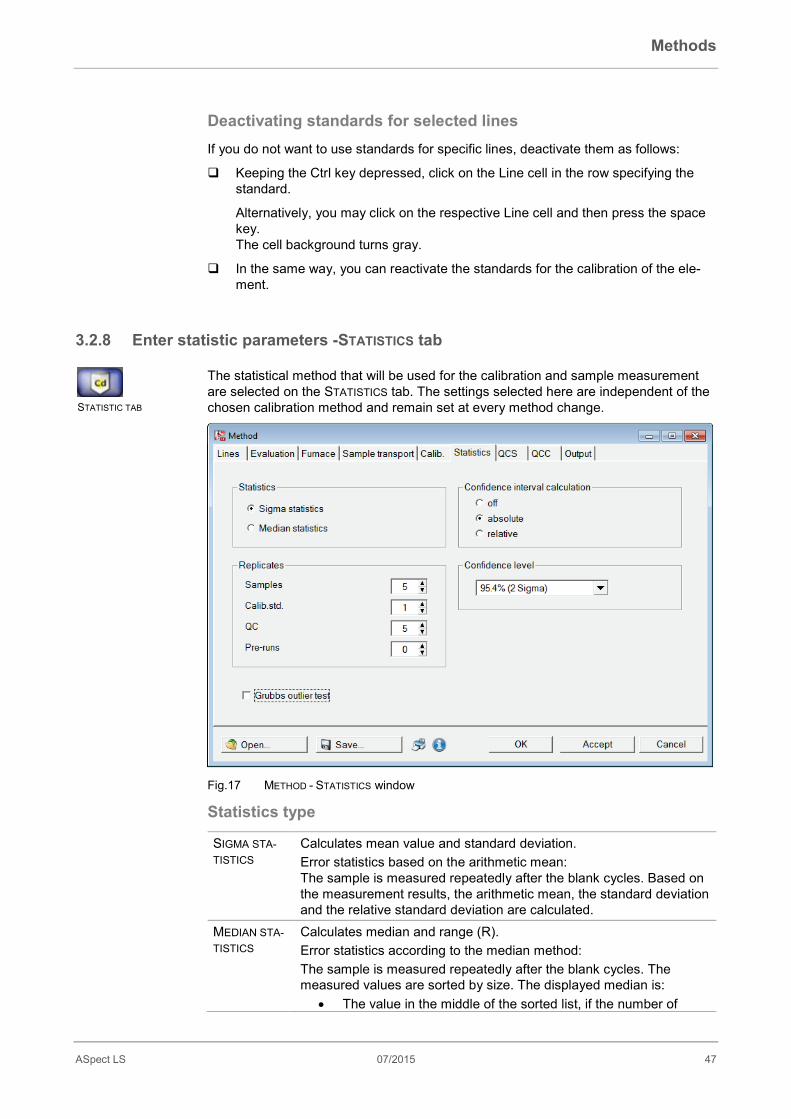
Methods
ASpect LS 07/2015 47
Deactivating standards for selected lines If you do not want to use standards for specific lines, deactivate them as follows:
Keeping the Ctrl key depressed, click on the Line cell in the row specifying the standard.
Alternatively, you may click on the respective Line cell and then press the space key. The cell background turns gray.
In the same way, you can reactivate the standards for the calibration of the ele-ment.
3.2.8 Enter statistic parameters -STATISTICS tab The statistical method that will be used for the calibration and sample measurement are selected on the STATISTICS tab. The settings selected here are independent of the chosen calibration method and remain set at every method change.
Fig.17 METHOD - STATISTICS window
Statistics type
SIGMA STA-TISTICS
Calculates mean value and standard deviation. Error statistics based on the arithmetic mean: The sample is measured repeatedly after the blank cycles. Based on the measurement results, the arithmetic mean, the standard deviation and the relative standard deviation are calculated.
MEDIAN STA-TISTICS
Calculates median and range (R). Error statistics according to the median method: The sample is measured repeatedly after the blank cycles. The measured values are sorted by size. The displayed median is:
• The value in the middle of the sorted list, if the number of
STATISTIC TAB

Methods
48 07/2015 ASpect LS
measurement cycles is odd.
• The mean value of the two measured values in the middle of the sorted list.
As the smallest and largest individual measured values do not influ-ence the measurement result, the median statistics are suitable for the elimination of outliers.
Number of replicate measurements
SAMPLES Number of repeat measurements per sample CALIB.-STD
Number of repeat measurements per calibration sample
QC Number of repeats per QC measurement (types of QC measurement see also section “Specify quality control samples for QC tabs - QCS tab” pg. 49”.
PRE-RUNS
Number of pseudo measurements. Number of sample measurements preceding the statistics series, but disregarded for the calculation of the measurement result.
Grubbs outlier test This function is provided for mean value statistics with at least three repeat measure-ments per sample.
DEACTIVATED Includes all values of the statistics series for the determination of the mean value.
ACTIVATED Outliers are eliminated and excluded from the calculation of statistical quantities. The thus found mean values in the result table are marked by "!".
Confidence interval calculation The calculation of the confidence interval is based on the chosen statistical certainty (see below). In the calculation of the confidence interval, the errors in sample meas-urement and particularly the calibration errors are included, so that a value will be presented even if the statistics function has been deactivated.
OFF Confidence interval is not calculated. ABSOLUTE Displays the confidence level in absolute values (in concentration
units) RELATIVE Displays the confidence interval in relative values (in percent of the
concentration value) CONFIDENCE LEVEL
The confidence level (selectable between 68.3 ... 99.9%) is used for the calculation of the confidence interval of the samples and the prognosis ranges of the calibration curves.

Methods
ASpect LS 07/2015 49
3.2.9 Specify quality control samples for QC tabs - QCS tab Specify the QC samples for the quality control tabs in the window METHOD - QCS. The system of the QC control tabs serves to monitor quality over a long period of time. This involves the insertion of control measurements, with samples in predetermined positions during measurement. These control measurements should yield known re-sults. It is either the absolute value (absorbance/ concentration) or the concentration difference from the previous sample which is known.
The results of the quality control measurements are automatically recorded on so-called QC charts (also called quality rule charts or control charts). The tabs are saved with the method and continued for any further measurement with the method.
You may define various quality control samples (QC samples). The concentration and tolerance data for these samples are to be defined in the METHOD / QCS window.
Fig. 18 METHOD / QCS window
Elements of the QCS tab
TYPE QC sample the parameters of which (error limits and proce-dure selected) are displayed in the line list. You can select a QC sample from the list for viewing and edit-ing.
NAME Name of the displayed QC sample REACTION Procedure to be taken if the results of the QC sample exceed
or fall below the defined error limits. [NEW/CHAGE…] To be activated for defining a new or modifying an existing QC
sample. [DELETE ] Deletes the displayed QC sample. BLANK CORRECTION Not accessible for QC standard and QC blank
Takes blank correction into account, if activated.
QCS TAB
Methods
50 07/2015 ASpect LS
UNIT List box for selecting the corresponding concentration unit. [QC SAMPLES OVER-VIEW]
Opens a list with the line-specific parameters of all QC sam-ples.
TABLE In the table, the parameters of the QC sample selected in the TYPE list box are displayed.
Entering parameters of QC samples To create a new parameter set for a QC sample or edit the currently displayed
one, click on [NEW/MODIFY...]. This will bring up the ADD/MODIFY QC SAMPLE TYPE window.
From the TYPE list, choose the sample type and, if you intend to define several QC samples of the same type, assign a number (e.g. QC-Std.2). The following sample types are selectable:
QC SAMPLE
Defines a sample as QC sample. The concentrations of the QC sample may either be loaded from the database or typed in directly. To recall a stored data record for the QC sample from the database, activate the FROM DATABASE option and choose the corresponding QC sample from the opposite list box (→ "Specifying stock standards and QC samples", pg. 160). Alternatively, you may type in the concentrations of the QC sample directly in the table on the QCS tab. In this case, activate the ENTER MANUALLY option. Max. number of QC samples: 50
QC STD.
Defines a standard as QC sample. You may use every standard as QC standard that has been defined in the calibration table (CALIB. tab). If the calibration standard was defined as being mixed by the autosampler, the QC standard will be mixed by the autosampler as well. The autosampler positions will be adopted from the CALIBRATION TABLE. The assigned number at the same time defines the used calibration standard e.g. "QC-Std.2" - the second calibration standard is used as a QC sample. Possible number of QC standards = number of standards in the cali-bration table (max. 65)
QC BLANK
Defines the blank as QC sample.
QC SPIKE
Defines a stock sample as QC sample. In recovery/addition, the measurement results of a defined concentra-tion addition to one or several samples are checked. To this end, a QC stock sample is to be defined after any sample in the sample ta-ble (QC-Stock sample = sample + addition with a solution of known concentration). After the measurement of sample and QC stock sam-ple, the concentration difference of both is compared with the "Ex-pected concentration growth” and the recovery rate calculated. When using the flame technique, the solution with added stock solution must have been pre-mixed.
If no certified quality control samples are available, quality control may also be carried out by means of double determinations:
Methods
ASpect LS 07/2015 51
QC TREND
The measured concentration value is stored when the quality control sample appears for the first time in the analytical procedure. When the QC sample appears the next time, the concentration difference is formed and evaluated. It is advisable to measure these QC samples at the beginning and at the end of a sample measurement series.
QC MATRIX
A sample to be analyzed is split before preparing the sample. Both portions are separately subjected to all steps of sample preparation. They are placed separately on the autosampler tray as QC Trend and QC Matrix. The difference between the determined concentrations is evaluated.
From the REACTION list box, choose the further procedure to be run if the error
limit is exceeded:
With QC SAMPLE, QC STD. and QC SPIKE selected as QC sample type:
FLAG The measured value is flagged in the sample table; the measure-ment program continues measuring the next sample.
RECAL. + CONTINUE
A recalibration is run. Afterwards, the QC-sample is re-measured. If the QC sample is now within the permissible range, the meas-urement is continued with the next sample; otherwise, the meas-urement program will be stopped.
CAL. + CONTINUE
A new calibration is run. Afterwards, the QC-sample is re-measured. If the QC sample is now within the permissible range, the measurement is continued with the next sample; otherwise, the measurement program will be stopped.
RECAL. + RERUN
A recalibration is run. Afterwards, the QC-sample is re-measured. If the QC sample is outside the range, the measurement program will be stopped. If it is within the range, all samples measured after the last QC sample or the last (re)calibration, will be re-measured. If the QC sample is again outside the permissible error limits, the measurement program will be stopped.
CALIB. + RERUN
A new calibration is run. Afterwards, the QC-sample is re-measured. If the QC sample is outside the range, the measure-ment program will be stopped. If it is within the range, all samples measured after the last QC sample or the last (re)calibration, will be re-measured. If the QC sample is again outside the permissible error limits, the measurement program will be stopped.
NEXT ELE-MENT
The current measurement program will be stopped and the meas-urement program of the next element started. This option is only available, if the method contains more than one line.
STOP The current measurement program will be stopped.
If you selected QC-BLANK as QC sample type, you may only choose among the FLAG, NEXT ELEMENT and STOP reaction options described above.
For the QC TREND and QC MATRIX QC sample types, no reaction is provided.
For the QC TREND and QC MATRIX QC sample types a blank value correction is provided as an option. For this purpose activate the check box BLANK VALUE.
In the list of QC samples, define the line-specific parameters for every element line dependent on the QC sample type selected:
LINE Name of element line

Methods
52 07/2015 ASpect LS
EXP. CONC. For QC Sample und QC Std. Expected concentration in QC sample.
EXP. CONC. IN-CREASE
For QC Stock. Expected concentration increase from sample to sample + ad-dition. Enter the value according to the added volume and the concen-tration of the spiking solution.
EXP. ABSORB-ANCE
For QC Blank. Absorbance expected in QC Blank.
LOW. DEVIATION [%]
Lower range of error limit in percent.
UP. DEVIATION [%]
Upper range of error limit in percent.
QC-CHART If marked by "+"sign, the result of the quality control for this line will be presented on the QC chart of the result list.
REACT.! If the error range limits are exceeded, the procedure selected from the REACTION list box shall be applied. If several lines have been marked by "+", it will do that the error limits are exceeded for one of these lines to start the selected reaction (OR logic).
UNIT Unit of the expected concentration (only with selected QC Std. option)
3.2.10 Specify quality control during the sequence - QCC tab In the window METHOD / QCC specify the parameters for the quality control during a sequence:
• relative standard deviation (mean value statistics) or relative range (median statistics),
• Calibration check and
• recalibration check and
• procedure to be run if error limits are exceeded.
You may choose various control options with different reactions simultaneously.
QCC TAB

Methods
ASpect LS 07/2015 53
Fig.19 METHOD–QCC window
Types of quality control
RSD/RR% CHECK
Check of relative standard deviation or relative range (→ "Enter sta-tistic parameters -STATISTICS tab", pg. 47).
CALIB. CHECK Check of calibration RECAL. CHECK Check of recalibration factor
Reactions if error limits are exceeded
NONE The corresponding check is not performed. FLAG Marks the corresponding sample, calibration or recalibration in the
sample table, if the error limits are exceeded. REPEAT + CONTINUE
Accessible only for RSD/RR% CHECK option. Repeats the measurement of the respective sample, if the serial preci-sion limit was exceeded, before the next sample is measured.
CAL. + CON-TINUE
Accessible only for CALIB. CHECK and RECAL. CHECK options. Runs a new calibration if the error limits for the calibration or the recal-ibration factor were exceeded. Afterwards, measurement is continued with the next sample.
NEXT ELE-MENT
Accessible only for CALIB. CHECK and RECAL. CHECK options. Stops the measurement of the currently running element line and starts measurement of the next element line, if the error limits were exceeded. This option is only available when the method contains more than one element line.
STOP Accessible only for CALIB. CHECK and RECAL. CHECK options. Stops the measurement of the currently running method, if the error limits were exceeded.

Methods
54 07/2015 ASpect LS
Graphite tube control Only for graphite tube technique.
Specify settings for graphite tube monitoring.
MAX. HEATING CY-CLES
Enter maximum number of measurements to be performed with the tube. The current value of the heating cycles is given in the adjacent field.
REACTION Select reaction type on reaching of maximum number of meas-urements: NO REACT. Graphite tube utilization is not monitored. FLAG Mark measurement in sample table when limit value
is exceeded. STOP Stops analytical procedure on exceeding limit value.
Line-specific parameters of quality checks In the table, enter the line-specific parameters of the various quality checks. You may define for every analysis line, whether it shall be considered for the check. If one or several of the checked lines exceed the error limit, the reaction chosen above will be released.
Quality check
Parameters Meaning
RSD/RR% CHECK
RSD/RR%<
The system will respond as selected if the relative standard deviations or the relative ranges are larger than or equal to the specified value. RSD! If the lines are marked by "+", the RSD%
or RR% will be checked. CALIB. CHECK
R2(ADJ.)>
The coefficient of determination R2(adj.) must be larger than or equal to the specified value. Otherwise, the system will respond as selected. R2! If the lines are marked by "+", R2(adjust)
will be checked. RECAL. CHECK
REC.FACT> Rec.Fact<
Upper limit of recalibration factor. Lower limit of recalibration factor. The selected response will be released, if the calibra-tion factors are outside these specified limits. REC.! If the lines are marked by "+", the recali-
bration factor will be checked.

Methods
ASpect LS 07/2015 55
3.2.11 Specify output and results table - OUTPUT tab On the OUTPUT tab specify the number of decimal places with which results are pre-sented on the screen and on the printouts, and the order of lines for an analysis of several elements on the printout.
In the table below, define the number of decimal places for the display and printout of absorbance and concentration values, and the order in which the anal-ysis lines shall appear on the printout.
Fig. 20 METHOD / OUTPUT window
OUTPUT TAB

Sequences
56 07/2015 ASpect LS
4 Sequences A sequence is based on a loaded method, which contains the information on the type of calibration, statistical analyses, quality control, etc.
The sequence contains the information on the samples and actions in their order of processing. Some sample describing data such as sample name and position on the sample tray may also be entered directly. For permanent storage, however, the sam-ple describing data must be saved as sample information file.
The meaning of buttons and symbols contained in the SEQUENCE window, which are also used in other windows of this application, are described in section "Frequently used control elements" pg. 8
4.1 Managing sequences Like methods, sequences are saved to a common database. When you save and open sequences, the database window is opened (→ "The database window", pg. 168).
4.1.1 Create new sequence To create a new sequence, activate menu command FILE NEW SEQUENCE to
open the SEQUENCE window.
Alternatively, you may open the window with the currently active sequence pa-rameters by using menu command METHOD DEVELOPMENT SEQUENCE or by a
click on the icon .
4.1.2 Save sequence In the SEQUENCE window, click on [SAVE].
Alternatively, you may activate menu command FILE SAVE SEQUENCE.
This will bring up the SAVE SEQUENCE window.
In the NAME textbox, type the desired sequence name. As default, "Sequence" and the current date are offered, e.g. "Sequence-08-15-05".
In the field CAT.: (category), you may optionally enter an additional identifier of three characters to facilitate later method search in the database.
In the DESCRIPTION textbox, you can optionally enter information on the se-quence.
Save the sequence with [OK].
On doing so, the sequence will be saved to the database. If you choose an existing sequence name, the existing method will not be overwritten, but a new version created in the database. To remove sequences from the database, you must explicit-ly delete them!
FILE / NEW SE-
QUENCE
METHOD DEVELOP-
MENT SEQUENCE
FILE SAVE SE-
QUENCE
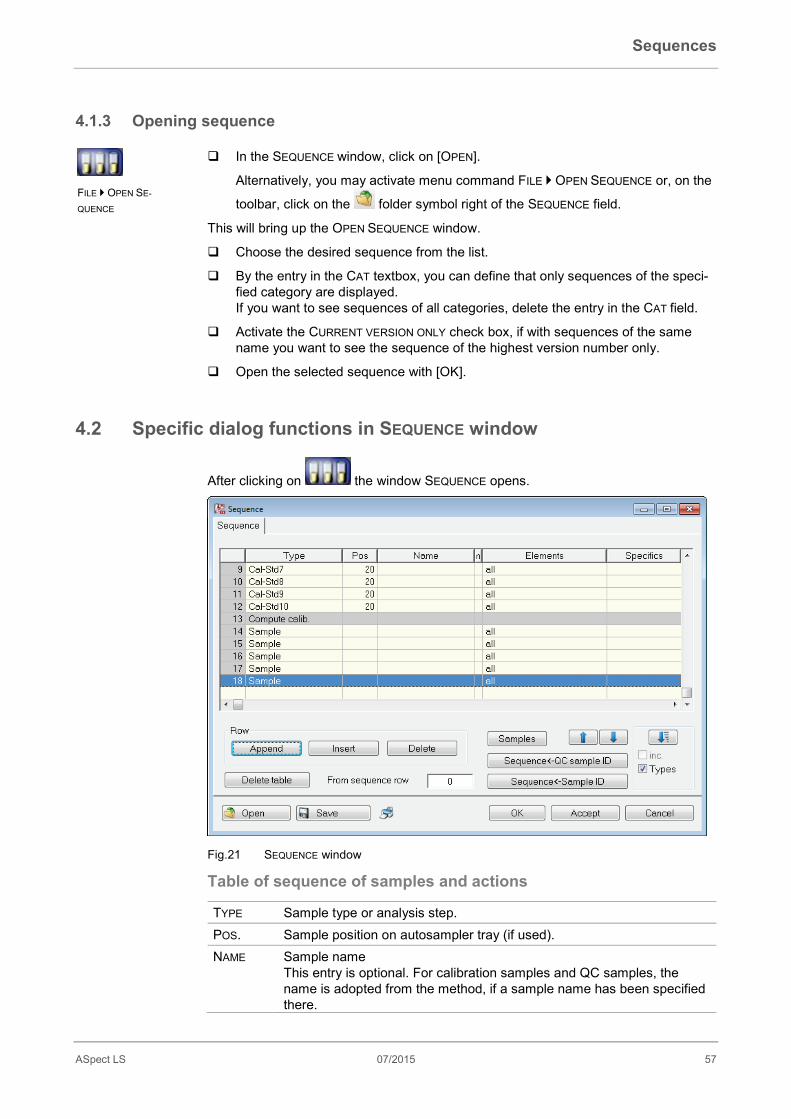
Sequences
ASpect LS 07/2015 57
4.1.3 Opening sequence In the SEQUENCE window, click on [OPEN].
Alternatively, you may activate menu command FILE OPEN SEQUENCE or, on the
toolbar, click on the folder symbol right of the SEQUENCE field.
This will bring up the OPEN SEQUENCE window.
Choose the desired sequence from the list.
By the entry in the CAT textbox, you can define that only sequences of the speci-fied category are displayed. If you want to see sequences of all categories, delete the entry in the CAT field.
Activate the CURRENT VERSION ONLY check box, if with sequences of the same name you want to see the sequence of the highest version number only.
Open the selected sequence with [OK].
4.2 Specific dialog functions in SEQUENCE window
After clicking on the window SEQUENCE opens.
Fig.21 SEQUENCE window
Table of sequence of samples and actions
TYPE Sample type or analysis step. POS. Sample position on autosampler tray (if used). NAME Sample name
This entry is optional. For calibration samples and QC samples, the name is adopted from the method, if a sample name has been specified there.
FILE OPEN SE-
QUENCE
Sequences
58 07/2015 ASpect LS
For samples to be analyzed, the names can be transferred from the sample information file.
NAME (2) Additional designation for sample identification (optional). ELEMENTS Only for methods with multiple elements
Select the elements/element lines which should be analyzed in a sample or conducted for the special actions. "ALL" All elements/element lines defined in the method will be de-
termined (default). ELEMENT SYMBOL
Only the specified elements will be determined, e.g. Cu, Pb ELEMENT SYMBOL + INDEX (for the analysis of several lines of an element)
Only the specified element lines will be determined, e.g. Cu1,Cu2.
"NOT" ELEMENT SYMBOL The specified elements will not be determined, e.g. not Cu,Pb.
"NOT" ELEMENT SYMBOL + INDEX The specified element lines will not be determined, e.g. not Cu1,Pb2.
SPECIFICS This field is not used so far. Control buttons
[APPEND] Appends a new row to the end of the list and opens the EDIT SE-QUENCE window.
[INSERT] Inserts a new row at the selected place of the list. [DELETE ] Delete marked lines. [DELETE TABLE] Deletes the complete sequence table. [SEQU.<-QC-SAMPLES]
Transfers QC sample information (e.g. names and sampler posi-tions) to window SAMPLE ID/ QC-SAMPLE INFORMATION (→ "Sample information data" p. 62). The information from the QC sample ID table are entered in the sequence table. The first row with the new sample ID is to be de-fined in the FROM ROW field.
[SEQUENCE<-SAMPLE]
Take information about sample names and place in the automatic sampler from the window SAMPLE-ID (→ "Sample information da-ta" p. 62). The information from the sample ID table is entered in the se-quence table. The first row with the new sample ID is to be de-fined in the FROM ROW textbox.
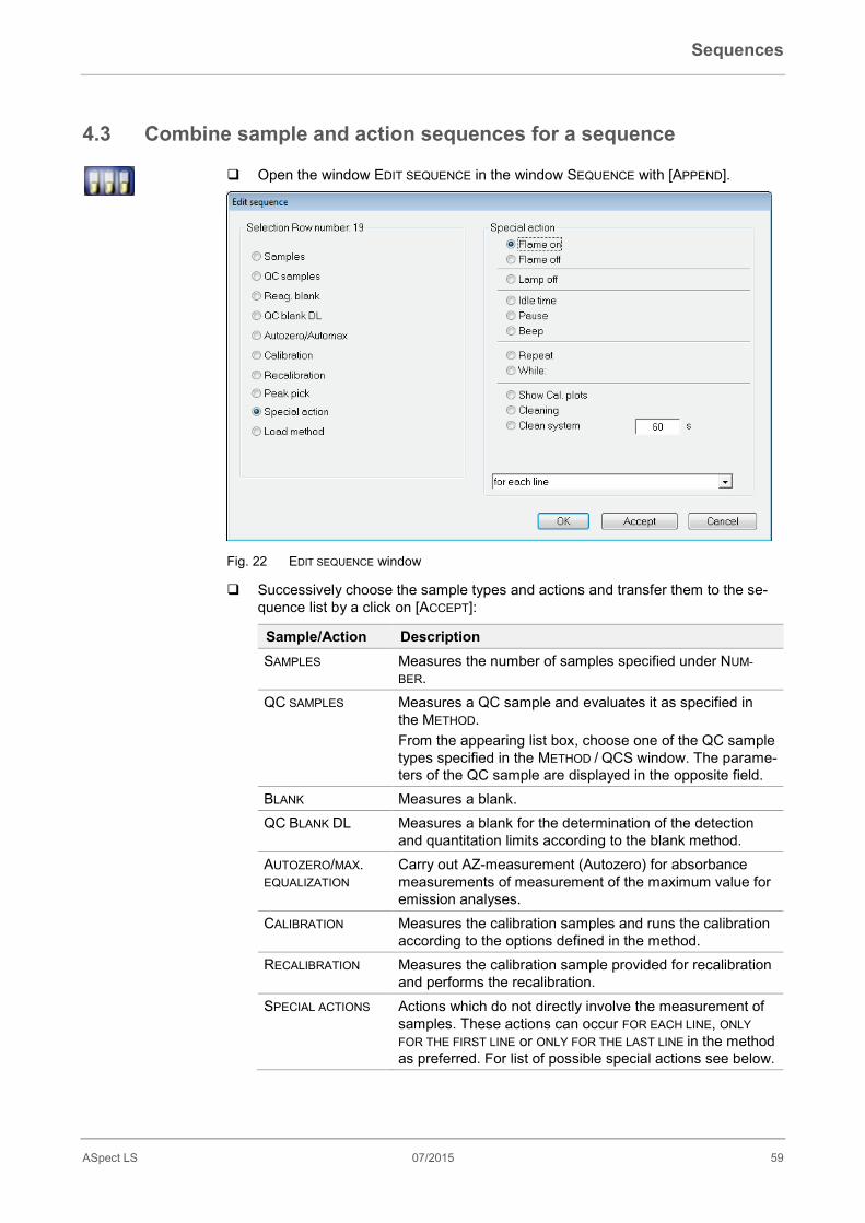
Sequences
ASpect LS 07/2015 59
4.3 Combine sample and action sequences for a sequence Open the window EDIT SEQUENCE in the window SEQUENCE with [APPEND].
Fig. 22 EDIT SEQUENCE window
Successively choose the sample types and actions and transfer them to the se-quence list by a click on [ACCEPT]:
Sample/Action Description SAMPLES Measures the number of samples specified under NUM-
BER. QC SAMPLES Measures a QC sample and evaluates it as specified in
the METHOD. From the appearing list box, choose one of the QC sample types specified in the METHOD / QCS window. The parame-ters of the QC sample are displayed in the opposite field.
BLANK Measures a blank. QC BLANK DL Measures a blank for the determination of the detection
and quantitation limits according to the blank method. AUTOZERO/MAX. EQUALIZATION
Carry out AZ-measurement (Autozero) for absorbance measurements of measurement of the maximum value for emission analyses.
CALIBRATION Measures the calibration samples and runs the calibration according to the options defined in the method.
RECALIBRATION Measures the calibration sample provided for recalibration and performs the recalibration.
SPECIAL ACTIONS Actions which do not directly involve the measurement of samples. These actions can occur FOR EACH LINE, ONLY FOR THE FIRST LINE or ONLY FOR THE LAST LINE in the method as preferred. For list of possible special actions see below.
Sequences
60 07/2015 ASpect LS
LOAD METHOD Load a saved method, e.g. in order to start another ele-ment analysis within sequence. With [...] open the window OPEN METHOD(→ "Opening methods" pg. 18). Select one of the two saved methods.
The following special actions can also be inserted in the measurement process:
LAMP, OFF Switch off hollow cathode lamp. PAUSE Stop the analysis. The sequence can subsequently be con-
tinued with the menu command ROUTINE / CONTINUEor . WAITING TIME Wait the time indicated under MIN. and then continue with
the analysis (e.g. while burning in the nitrous oxide flame). In the event of methods with multiple elements, the ele-ments/element lines can be selected in the sequence list for which the waiting period was complied with.
DISPLAY CALIBRA-TION FUNCTIONS
Display the calibration curve during the sequence in pro-gress.
BEEP Allow the PC to generate a signal tone, e.g. in order to indi-cate the end of the calibration. (Requires a sound card and loud speaker.)
CLEANING Carry out controlled cleaning. (→ “Set auto sampler - SAMPLE TRANSPORT tab” pg. 31)
FLAME OFF/ON Only flame technique Light/extinguish flame.
CLEAN FURNACE Only graphite tube technique Additional clean out step to clean the graphite tube. The graphite tube is heated to a predefined temperature once. Parameter settings for this clean out step can be made in the METHOD - FURNACE window (→ "Enter furnace program - FURNACE tab" pg. 25)
FORM TUBE Graphite tube technique and HydrEA technique: Form the graphite tube.
SYSTEM CLEAN-ING
Only hydride/hydrEA technique and flame technique Also clean hydride system. The parameters for this clean out step can be made in the METHOD - FURNACE window (→ "Specify Hydride and HydrEA systems" pg. 27) Clean autosampler AS 51/52s. For the flame technique the cleaning time is entered in the window METHOD - SAMPLE SUPPLY (→ "Auto sampler for flame and hydride/HydrEA technique" pg. 31).
LOAD SYSTEM Only Hydride/HydrEA technique Following a new installation or cleaning of the hydride sys-tem as should occur daily at the end of work, the tubes must be loaded with reagents before starting the analyses. There-fore this action should occur in the sequence before the first measurement.
Sequences
ASpect LS 07/2015 61
REPEAT/WHILE Loop through a part of the sequence until the action WHILE is reached. The number of cycles or a time interval in minutes can be specified as break condition. A sequential value is appended to the results records for identification. If the option AUTO. is active, requests for sample dosing in manual mode are suppressed.
After you have selected all actions of the sequence, return to the SEQUENCE win-
dow by clicking [OK].
Enter the ELEMENTS to be examined in the list ELEMENTS.
When using an autosampler: Set the position of the samplers in the sample changer. The positions of calibra-tion and QC samples are automatically taken from the method. However you can change the positions here.
Note
The data of the samples to be examined should best be entered in the window Sam-ple-ID and subsequently transferred into the sequence list (→ "Specify information data for samples and QC samples" pg. 65).

Sample information data
62 07/2015 ASpect LS
5 Sample information data
5.1 Manage sample information data
5.1.1 Generate new set of sample information data
Open the SAMPLE-ID window by a click on the symbol .
Alternatively, you may open the Sample ID window using the menu commands METHOD DEVELOPMENT SAMPLE ID or FILE NEW SAMPLE INFORMATION DATA.
5.1.2 Save sample information data Sample information is saved in CSV format which can be edited with spreadsheet software, e.g. MS Excel.
There are different ways to give the command for saving the current sample infor-mation.
In the SAMPLE ID window, click on [SAVE].
Alternatively, you may activate menu command FILE / SAVE / SAMPLE INFOR-MATION.
This will bring up the standard SAVE AS... dialog.
In the FILE NAME field, enter the desired name for the sample information file.
Save it by a click on [OK].
5.1.3 Open sample information data In the SAMPLE ID window, click on [OPEN].
Alternatively, you may activate menu command FILE OPEN SAMPLE INFORMATION FILE.
This will bring up the standard OPEN window.
Choose the desired file from the list and open it with [OK].
METHOD DEVELOP-
MENT SAMPLE-ID...
FILE NEW SAMPLE
INFORMATION FILE
FILE SAVE SAM-
PLE INFORMATION...
FILE OPEN SAMPLE
INFORMATION FILE...

Sample information data
ASpect LS 07/2015 63
5.2 Specific dialog functions in the SAMPLE-ID window
Fig.23 SAMPLE ID / SAMPLE INFORMATION window
The program pops up brief information windows on the table while you move the mouse pointer across the button.
Sample information tab The tab SAMPLE INFORMATION contains a list of the samples and their characteristics.
POS. Position of sample on autosampler NAME Sample name
This entry is optional. Maximum number of characters: 20
PRE-DF Pre-dilution factor. Factor by which the original sample was diluted be-fore being placed on the autosampler or supplied to the spectrometer, if no autosampler is used. The factor is required for the calculation of the concentration of the original sample.
UNIT Concentration unit of sample. WT.[G] Only for solution analytics
Weighed portion in grams. The weight of the original sample, which was dissolved in sample prepa-ration (in mL). The entry of the weight is required for the calculation of the concentration of the original sample (CONC.2 in the result table). NOTE: For solid analytics, known weighed sample portions must be specified in the RESULT WINDOW / SOLID TAB or weighed before the meas-urement of unknown sample weights (→ "Measure solid samples" pg. 83).
VOL.[ML] Volume of solvent used to dilute the weighed sample portion (in mL). The entry of this value is required for the calculation of the concentration of the original sample (CONC.2 in the result table).

Sample information data
64 07/2015 ASpect LS
NAME (2) Additional sample name. The entry is optional. Maximum number of characters: 20
AS-DF Dilution factor of the autosampler. NOTE: The dilution mode used here is set in the window Method - Sam-ple Supply (→ "Auto sampler for flame and hydride/HydrEA technique" pg. 31, "Autosampler for graphite tube technique (solution analytics)" pg. 34)
BLANK CORR.
Only for sample type SAMPLE Blank correction. OFF No blank correction performed. ON For the calculation of the concentration of the original sam-
ple, the blank measured last in the sequence will be sub-tracted.
SAMPLE TYPE
Select sample type reagent blank or sample. The sample-ID data are mapped to the sequence entries according to the sample type, e.g.: First reagent blank in sample-ID → First reagent blank in sample-ID Second reagent blank in sample-ID → Second reagent blank in sample-ID First sample in sample-ID → First sample in sample-ID Second sample in sample-ID → Second sample in sample-ID, etc.
Control buttons
[APEND] #-Insert number of new rows at the end of the list. [INSERT] #-Insert number of new rows at the selected place in the list. [DELETE ] Delete the marked row. NUMBER Input field for the entry of the number of rows to be inserted, or de-
leted. [DELETE TABLE] Deletes the complete table of sample information. [SAMPLE ID -> SEQUENCE]
Transfers sample names and positions on autosampler from the SAMPLE INFORMATION tab to the sequence list. In the FROM SE-QUENCE ROW input field, define the first row to be transferred.
[SEQUENCE -> SAMPLE ID]
Transfers sample names and positions on autosampler from the to the SAMPLE INFORMATION tab. In the FROM SEQUENCE ROW input field, define the first row to be transferred.
QC sample information tab The QC samples are shown on this chart analogous to SAMPLE INFORMATION tab.
The columns correspond to the columns of the tab Sample information. Additionally the column TYPE contains information about the QC type. The column UNIT is omitted because QC sample units are defined in the method.
Blank correction is not available for QC samples.
Control button
[QC SAMPLES -> SE-QUENCE]
Transfers QC sample names and positions on autosampler to the sequence list.

Sample information data
ASpect LS 07/2015 65
The meaning of buttons and symbols contained in the SAMPLE ID window, which are also used in other windows of this application, are described in Section "Frequently used control elements" pg. 8.
5.3 Specify information data for samples and QC samples Enter the Sample-ID in the window SAMPLE-ID / SAMPLE INFORMATION.
1. Then enter the corresponding number of samples to be analyzed in the field NUMBER. Then click on [APPEND] in order to insert the corresponding number of rows into the list.
2. In the table, enter the required information for every sample.
3. If the entries to be made in a column are identical, you may copy the entry of the selected cell to all following cells of the column by clicking on . If you activate the INC. check box, the value to be copied will be incremented by one each in copying it to the next cell. In this way, you can easily e.g. assign suc-cessive places on the tray of the autosampler or number a sample name consec-utively.
4. Texts in input fields can be copied to the Windows clipboard and pasted from there by using menu commands EDIT / COPY and EDIT /PASTEor shortcut keys [CTRL+C] and [CTRL+V].
5. When you entered all information required, specify in the FROM SEQUENCE ROW field from which row on you want to transfer sample information to the sequence. Then, transfer the data by a click on [SAMPLE ID-> SEQUENCE].
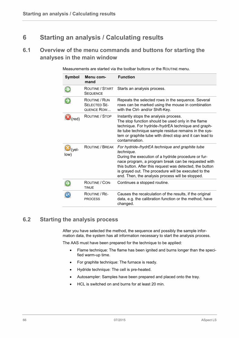
Starting an analysis / Calculating results
66 07/2015 ASpect LS
6 Starting an analysis / Calculating results
6.1 Overview of the menu commands and buttons for starting the analyses in the main window
Measurements are started via the toolbar buttons or the ROUTINE menu.
Symbol Menu com-mand
Function
ROUTINE / START SEQUENCE
Starts an analysis process.
ROUTINE / RUN SELECTED SE-QUENCE ROW...
Repeats the selected rows in the sequence. Several rows can be marked using the mouse in combination with the Ctrl- and/or Shift-Key.
(red) ROUTINE / STOP Instantly stops the analysis process. The stop function should be used only in the flame technique. For hydride-/hydrEA technique and graph-ite tube technique sample residue remains in the sys-tem or graphite tube with direct stop and it can lead to contamination.
(yel-low)
ROUTINE / BREAK For hydride-/hydrEA technique and graphite tube technique. During the execution of a hydride procedure or fur-nace program, a program break can be requested with this button. After this request was detected, the button is grayed out. The procedure will be executed to the end. Then, the analysis process will be stopped.
ROUTINE / CON-TINUE
Continues a stopped routine.
ROUTINE / RE-PROCESS
Causes the recalculation of the results, if the original data, e.g. the calibration function or the method, have changed.
6.2 Starting the analysis process After you have selected the method, the sequence and possibly the sample infor-mation data, the system has all information necessary to start the analysis process.
The AAS must have been prepared for the technique to be applied:
• Flame technique: The flame has been ignited and burns longer than the speci-fied warm-up time.
• For graphite technique: The furnace is ready.
• Hydride technique: The cell is pre-heated.
• Autosampler: Samples have been prepared and placed onto the tray.
• HCL is switched on and burns for at least 20 min.

Starting an analysis / Calculating results
ASpect LS 07/2015 67
Saving analysis results during the analysis process The results of the analysis are saved to a database in the default folder or a user-defined subfolder directly during the measurement. They may be saved optionally to a new database or added to an existing database. However, it is not possible to over-write a result database by selection of the same name.
Fig. 24 MEASUREMENT START SEQUENCE window
The target for result storage will be requested automatically at the start of a measure-ment routine. This will bring up the MEASUREMENT START SEQUENCE WINDOW: SE-QUENCE NAME with the following options for the result file:
NAME Here, enter the desired name for the result database. NEW FILE/LIST If activated, you must enter a new file name.
The program checks if the file name exists already. Existing files cannot be overwritten.
APPEND TO FILE/LIST New results will be appended to the existing results file. With [...] you can open the se-lection dialog. Choose an existing results file from the displayed list.
FOLDER Choose the save path for the results file. DESCRIPTION Here, you may enter an additional comment that is saved
along with the analysis results. The entry is optional.
SWITCH OFF LAMP AFTER ERROR STOP
When the measurement is stopped because of an error the HCL is automatically switched off.
[OK] Starts the measurement.
The file contains the results of measurement and evaluation and the sample ID infor-mation. In addition the method parameters are saved in the result database.
The result database is saved with the extension ".tps".

Starting an analysis / Calculating results
68 07/2015 ASpect LS
Starting measurements Start the measurement routine using menu command ROUTINE / START SE-
QUENCEor click on .
In the START SEQUENCE window, choose a file name for the results file. You may optionally save the result to a new file or append it to an existing file. Overwriting of an existing file is not possible.
After you selected the file name, the measurement routine will start according to the settings selected in the method and the sequence.
If you use an autosampler, the measurement runs automatically. In the case of manual sample feed without autosampler, follow the prompts for the provision of samples displayed on the screen.
Note
In the event of methods with multiple elements, the processing of the sequence takes place in accordance with the order of the elements and/or element lines in the method. As a result, the first element for the sequence is fully processed before the sequence begins again with the second element. The measurement of certain elements can be ruled out or agreed upon for individual samples in the sequence. Waiting times can also be added based on the element (Column ELEMENTS in the sequence table, sec-tion "Specific dialog functions in SEQUENCE window” pg. 57).
Displays during the analysis process While the measurement is running, the results are displayed in real time in the main window.
Additionally, the following windows may be displayed on the screen: SIGNAL PLOT, FLAME REPORT and CALIBRATION CURVE. The display of these windows is to be selected in the OPTIONS / ANALYSIS SEQUENCE window (→ "Options for analysis sequence", pg. 157). You may also optionally hide these windows during the measurement.
To open the display windows, use menu command VIEW OPEN DISPLAY WIN-DOWS or function key F7.
To close the display windows, use menu command VIEW CLOSE DISPLAY WIN-DOWS or function key F8.
In the sequence list of the main window, the measurement progress is logged. The rows with the successive actions are marked by the following symbols in the table column:
- Not measured/executed yet.
Ο Just being measured.
+ Already measured/executed. Additionally, in the symbol bar at the side large buttons are displayed during meas-urements:
[ACTIVATE SCRAPER]
The scraper cleans the burner head between two measurements within a statistics series of a sample.
[SHOW METH-OD]
Turns the method window on. A method can only be read, it cannot be changed.
ROUTINE / START
SEQUENCE
VIEW OPEN DIS-
PLAY WINDOWS
… CLOSE DISPLAY
WINDOWS

Starting an analysis / Calculating results
ASpect LS 07/2015 69
[SEQUENCE SAMPLES]
Turns the sequence window on. A sequence may be expanded while measurement is going on. The sequence window includes a [SAMPLE ID] control button that allows you to edit further sample ID data.
[STOP SE-QUENCE]
Instantly stops the analysis process.
[RESULT WIN-DOWS]
Display or close the display window (analogous to the menu com-mands VIEW / OPEN DISPLAY WINDOWS and VIEW / CLOSE DISPLAY WINDOWS).
[EXTINGUISH FLAME]
Extinguishes the flame.
6.3 Interrupting, stopping, continuing the analysis process Analysis processes can be interrupted and continued later. However, when using the graphite tube technique and the hydride technique the currently running sample measurement should be finished first and only the analysis process stopped. This procedure is to prevent sample residues from being deposited in the graphite tube or hydride system. In flame analyses, you may stop the process at any time.
With menu command ROUTINE STOP or button (red button), you can stop the analysis process instantly.
With menu command ROUTINE BREAK or button (yellow button), you can request for an interruption of the analysis process. After this request was detect-ed, the button is grayed out. The currently running hydride program or furnace program will be finished first. Then, the analysis process will be stopped. (For hy-dride technique and graphite tube technique)
With menu command ROUTINE CONTINUE... or the button, you can continue a stopped/interrupted routine. This will bring up the CONTINUE SEQUENCE dialog, in which you are informed of the status of actions before the interruption. If you want to modify the method before continuing, activate the CONTINUE WITH MODIFIED METHOD check box. On doing so, a new method entry is made to the re-sults file. The measurement may be continued in one of the following ways:
CONTINUE Repeat current sample, current line and current statistical run.
FIRST STATISTICAL RUN
Continue with current sample, current line and the first statistical run.
NEXT ELEMENT Continue with first sample, next element. FROM TABLE ROW Continue with the table row displayed in the text box.
ROUTINE STOP
… BREAK
… CONTINUE

Starting an analysis / Calculating results
70 07/2015 ASpect LS
6.4 Repeat the actions of the sequence Single actions in a sequence, single measurements in statistic runs or special actions can be repeated.
In the main window on the SEQUENCE/RESULTS or the SEQUENCE tab, select the row with the action to be repeated.
Start the measurement routine with menu command ROUTINE / RUN SELECTED SEQUENCE ROW... or a click on
.
In the START SEQUENCE window, choose a file to which the result of the repeated measurement shall be saved. You may optionally save the result to a new file or append it to an existing file. Overwriting of existing results by selection of the same file name is not possible.
After you selected the file, the selected action will be repeated.
For each repeated sequence start or row measurement a new method version is saved with the results data even if the method parameters have not been changed.
6.5 Reprocessing analysis results After any change of evaluation conditions, such as a change of the calibration func-tion, method, etc., the results must be recalculated to take these changes into ac-count.
Likewise, it is possible to change sample information data, such as sample names and dilution factors, and have them taken into account for the presentation of analysis results.
Activate menu command ROUTINE / REPROCESS... or click on . This will bring up the REPROCESS RESULTS window.
In this window, make the following entries:
NAME Name of original file with analysis results. MODIFIED SAMPLE INFORMATION DATA
Sample information data were changed and shall be up-dated in reprocessing.
ALLOW QC TAB EN-TRIES
Enter recalculated values on the QC tabs if QC tabs are specified in the method.
REPROCESSED EN-TRIES
Causes reprocessing of the entries in the result list cover-ing the rows specified in the FROM and TO fields.
DESCRIPTION Additional remark saved along with the reprocessed analysis results. The entry is optional.
RESULT FILE (TAR-GET)
FOLDER Choose the save path for the results file.
ROUTINE / RUN
SELECTED SE-
QUENCE ROW...
ROUTINE / REPRO-
CESS...
Starting an analysis / Calculating results
ASpect LS 07/2015 71
NAME Enter the file name for the results file. NEW FILE/LIST If activated, you must enter a new file
name. The program checks if the file name exists already. Existing files cannot be over-written.
APPEND TO FILE/LIST New results will be appended to the existing results file. With [...] you can open the selection dialog. Choose an existing re-sults file from the displayed list.
UPDATE RESULT PLOTS
After reprocessing the result plots will be uppdated.
Confirm the selection of the results file with [OK] and start the reprocessing ac-
tion.
Note
Reprocessed values may be optionally saved to a new database or appended to an existing results file. Manipulation of the original data is ruled out. The original results always remain as long as the original file is not deleted.
6.6 Evaluating measurements parallel to running analyses While measurements are running, it is impossible to evaluate results in the same pro-gram instance. However, it is possible to start a second program instance of the appli-cation in offline mode, while measurements are running in the first instance. In this mode, there is no communication with the device. However, all other functions such as developing methods or loading and analyzing results can be used parallel to the run-ning measurements of the first program instance.
Start ASpect LS in the second instance by menu command FILE START OFFLINE.
Open the results file of the running measurement using menu command FILE OPEN RESULTS. The results measured so far will be loaded in the result window.
Further results of the running measurement can be loaded via menu command VIEW UPDATE RESULTS LIST or the icon button
.
You may further process the results, e.g. by loading sample details or the calibra-tion function (→ "Displaying details of single values of samples" pg. 78, "Calibration" pg. 87).
NOTE
In reprocessing, the recalculated results are saved to a new database. It is not possi-ble to access the original results file.
FILE START OF-
FLINE FILE OPEN RE-
SULTS…
VIEW UPDATE
RESULT LIST

Starting an analysis / Calculating results
72 07/2015 ASpect LS
6.7 Displaying results and analysis progress in the main window
Important note
Depending on the selected operating mode, the measured values are determined in absorbance or emission. In the following, only absorbance values will be mentioned. The same specifications and information, however, also applies to emission values. In numerical presentation of data, the abbreviation ABS is used for absorbance values and EMS for emission values.
The measurement results and the sequence are extensively displayed in the main window in the background of the workplace.
The presentation on different tabs in the main window provides a good overview of measurement results and statistical analyses.
The following tabs are selectable:
• Sequence/Results (Content of the Sequence and Results tabs on one tab)
• Sequence (displays the current sequence)
• Results (presentation of measurement results)
• Overview (summary of measurement results)
• Solids (preparation of the solid samples for analysis)
The status bar of the result window shows the file name of the current results file.
6.7.1 SEQUENCE/RESULTS tab The SEQUENCE/RESULTS tab contains the data of both tables SEQUENCE and RESULTS (→ "SEQUENCE tab", pg. 72, "RESULTS tab" pg. 73).
6.7.2 SEQUENCE tab On the SEQUENCE tab, the active sequence is listed.
On this tab, you can follow the progress of the running analysis. The various samples and special functions are marked in the first column of the table as follows:
- Not measured/executed yet.
Ο Just being measured.
+ Already measured/executed.
Note
After the measurement, you can remeasure a selected sample. To this end, you must
have marked the sample row in the sequence. Then, click on on the toolbar.
Starting an analysis / Calculating results
ASpect LS 07/2015 73
6.7.3 RESULTS tab The RESULTS tab shows all measurement results and statistical analyses. The values are split up in further tables for a clear presentation. The index tabs for these tables are arranged at the bottom edge of the window.
The values are sorted by the order of sample measurement. For every sample, the analyzed elements are listed.
Abs./Time table The table contains the absorbance values and the statistical analyses according to the selected method options (METHOD - QCC window).
NO. Number in analysis sequence. NAME Sample name LINE Element line ABS. Mean value of measured individual absorbance values
For solid analytics: normalized absorbance
SD Standard deviation (mean value statistics) RSD% Relative standard deviation (mean value statistics) DATE/TIME Date and time of measurement INDIVIDUAL VALUES ABS. (EMS.)
Single values of absorbance measurements (emission measurement)
Table L-Abs. The table contains the absorbance values and the statistical analyses according to the selected method options like the table Abs./Time (METHOD /- QCC window).
Solids Table
NO. Number in analysis sequence. NAME Sample name LINE Element line NORM. ABS. Mean value of the standardized absorbance (absorbance /
weighed portion) SD Standard deviation of Conc. 1 (mean value statistics) RSD% Relative standard deviation of Conc. 1 (mean value statistics) MASS Mean absolute analyte mass UNIT. Absolute unit of the analyte HUM [%] Relative moisture of the sample. WT. [MG] Weights for all individual amounts DATE/TIME Date and time of measurement INDIVIDUAL VALUES (ABS.)
Single values of absorbance measurements

Starting an analysis / Calculating results
74 07/2015 ASpect LS
Conc.1 table The CONC.1 table shows the analyzed concentrations of the samples as supplied to the AAS.
NO. Number in analysis sequence. NAME Sample name LINE Element line UNIT Concentration unit CONC.1 Analyzed concentration of sample SD Standard deviation of Conc. 1 (mean value statistics) RSD% Relative standard deviation of Conc. 1 (mean value statistics) R Range of Conc. 1 (Median statistics) R% Relative range of Conc. 1 (Median statistics) CF Confidence interval REM. Notes
(→ " / Overview of markings used in the display of values" pg. 188) DF Dilution factor if concentration is exceeded
In the method, you can define automatic dilution by the autosampler if the concentration is exceeded (→ "Auto sampler for flame and hy-dride/HydrEA technique" pg. 31 and "Autosampler for graphite tube technique (solution analytics)" pg. 34). The dilution factor of this au-tomatic dilution procedure by the autosampler is considered for the calculation of CONC.1.
ABS. Mean value of measured individual absorbance values For solid analytics: normalized absorbance
SD(ABS.) Standard deviation of absorbance values (mean value statistics) DATE/TIME Date and time of measurement INDIVIDUAL VALUES ABS. (EMS.)
Single values of absorbance measurements
Conc.2 table The CONC.2 table shows the concentrations of the original samples. In calculating CONC.2, the sample information data (see SAMPLE ID table below) are considered:
• Pre-dilution
• Weighed portion of solids
• Conversion factors for other units
NO. Number in analysis sequence. NAME Sample name LINE Element line UNIT Concentration unit CONC.2 Concentration of original sample taking sample infor-
mation data into account SD2 Standard deviation of Conc. 2 (mean value statistics)

Starting an analysis / Calculating results
ASpect LS 07/2015 75
RSD% Relative standard deviation of Conc. 2 (mean value statis-tics)
CF Confidence interval of Conc. 2 REM. Notes
(→ " / Overview of markings used in the display of values" pg. 188)
ABS. Absorbance value For solid analytics: normalized absorbance
SD(ABS.) Standard deviation of absorbance values (mean value sta-tistics)
R(ABS.) Range of absorbance values (median statistics) DATE/TIME Date and time of measurement INDIVIDUAL VALUES ABS. (EMS.)
Single values of absorbance measurements
QC Res. table The QC RES. table shows the results of QC samples: Rated and actual values of con-centration, recovery rates (not for blank) and reactions to possible deviations (all types except blank).
NO. Number in analysis sequence. NAME Sample name LINE Element line QC (FOR CALIBRA-TION FUNCTIONS)
R2(ADJ.) Slope Char. Conc. – Characteristic concentration
QC (FOR QC SAM-PLES, NOT FOR QC BLANK)
CONC.1 Rated value Recovery rate
With QC samples and QC Std., the recovery rate of concentration is determined. With QC-Stock, QC-Trend and QC-Matrix, the re-covery rate of the concentration increase caused by additions is determined.
QC (FOR BLANK DE-TECTION LIMIT)
SD Standard deviation of blank measurements CRDL Detection limit LOQ Limit of quantitation
REM. Notes about QC event (for example ">Cal.") (→ " / Overview of markings used in the display of values" pg. 188)
ABS. Mean value of measured individual absorbance values For solid analytics: normalized absorbance
SD(ABS.) Standard deviation of absorbance values (mean value statis-tics)
DATE/TIME Date and time of measurement INDIVIDUAL VALUES ABS. (EMS.)
Single values of absorbance measurements
Starting an analysis / Calculating results
76 07/2015 ASpect LS
Error table If errors occur during the measurements, the corresponding measurements are marked in red in all tables. In the ERROR table, the respective error is indicated in writ-ing.
Single val. table The SINGLE VAL. table contains the measured individual absorbance values.
Sample ID table The sample-ID table contains the sample information data (→ "Specific dialog func-tions in the SAMPLE-ID window" pg. 63).
NO. Number in analysis sequence. NAME Sample name LINE Element line TYPE Sample type POS. Position of sample on autosampler PRE-DF Pre-dilution factor. Factor by which the original sample was diluted be-
fore being placed on the autosampler or supplied to the spectrometer, if no autosampler is used. The factor is required for the calculation of the concentration of the original sample.
WT.[G] Only for solution analytics The weight of the original sample in grams, which was dissolved in sam-ple preparation (in mL). The weight is required for the calculation of the concentration of the original sample (CONC.2).
VOL.[ML] Volume of solvent used to dilute the weighed sample portion (in mL). This value is required for the calculation of the concentration of the orig-inal sample (CONC.2).
NAME (2) Additional sample name. AS-DF Dilution factor of the autosampler. BLANK CORR.
Blank correction. OFF No blank correction performed. ON For the calculation of the concentration of the original sam-
ple, the blank measured last in the sequence will be sub-tracted.
Table Energy set The table ENERGY SET displays an overview of the current instrument parameters.
NO. Number in analysis sequence. NAME Sample name LINE Element line PMT Photomultiplier voltage in V HC-AMPL. HC signal amplification BC-AMPL. Background correction amplification D2 CURRENT Deuterium lamp current in mA
Starting an analysis / Calculating results
ASpect LS 07/2015 77
USER DEFINED tab On the USER DEFINED tab you can select the parameters for the result display and their order in the table.
Click on the button [SELECT COLUMNS…] in the right lower corner of the table.
Select in the window SELECT COLUMNS the desired parameters.
To change the order in the result display, select the parameter and shift him with the keys and on the right position in the list. Several together select-ed parameters are shifted in the block
After the return in the main window the results are displayed. To change the width of a column move the mouse pointer to the corresponding border line in the col-umn head until it turns into a double-headed arrow. Keeping the left mouse button depressed, you can then drag the border line to adjust the desired width.
NOTE: The column width is stored in this view. Changes of the column width of the over ta-bles in the main window are reseated while closing the tables.
6.7.4 OVERVIEW tab On the OVERVIEW tab, the analysis results are summarized. You may choose among various presentation options:
• Conc. 1 – Concentration 1
• Conc. 2 – Concentration 2
• Abs.(RSD%/R%)– Absorbance (Relative Standard Deviation or Rela-tiveRange)
• Abs. – Absorbance
• LOD – Limit of Detection
• LOQ – Limit of Quantitation
• Recovery (rated value) - Recovery rate (rated value)
• R2(adj) – Correlation of the calibration curve
By activation of the respective check boxes, the following sample types can be dis-played:
• Samples
• QC samples
• Cal. Std.
• Other
opens then window PRINT OVERVIEW for printing the currently displayed data (→ "Print functions in ASpect LS" p. 163).
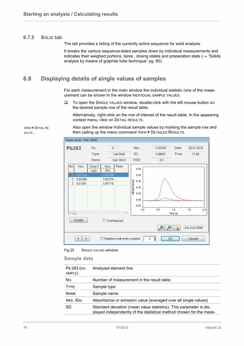
Starting an analysis / Calculating results
78 07/2015 ASpect LS
6.7.5 SOLID tab The tab provides a listing of the currently active sequence for solid analysis.
It breaks the various sequence-listed samples down by individual measurements and indicates their weighed portions, tares , dosing states and preparation state (→ ”Solids analysis by means of graphite tube technique” pg. 80).
6.8 Displaying details of single values of samples For each measurement in the main window the individual statistic runs of the meas-urement can be shown in the window INDIVIDUAL SAMPLE VALUES.
To open the SINGLE VALUES window, double-click with the left mouse button on the desired sample row of the result table.
Alternatively, right-click on the row of interest of the result table. In the appearing context menu, click on DETAIL RESULTS.
Also open the window Individual sample values by marking the sample row and then calling up the menu command VIEW DETAILED RESULTS.
Fig.25 SINGLE VALUES window
Sample data
PB 283 (EX-AMPLE)
Analyzed element line
NO. Number of measurement in the result table TYPE Sample type NAME Sample name ABS. /EM. Absorbance or emission value (averaged over all single values) SD Standard deviation (mean value statistics). This parameter is dis-
played independently of the statistical method chosen for the meas-
VIEW DETAIL RE-
SULTS...

Starting an analysis / Calculating results
ASpect LS 07/2015 79
urement (mean/median). RSD Relative Standard Deviation (mean value statistics). This parameter
is displayed independently of the statistical method chosen for the measurement (mean/median).
DATE/TIME Date and time of the measurement selected in the table Displaying / deleting single values The measured single values of the samples (statistic runs) are shown in the table.
NO. Number of single value within the sample measurement WT. [MG] For solid analytics:
Weighed portions of individual samples. ABS. Calculated absorbance of single value
For solid analytics: normalized absorbance
CONC. 1 Analyzed concentration of the sample as it was supplied to the AAS. Pre-dilutions and weighed portions were not yet taken into account.
ABS. BG Absorbance of the background REM. NONE The single value is included in the calculation of the
mean value of the sample #MAN. The value was manually excluded from the calculation
of the sample value #CORR. The value was automatically excluded from the calcu-
lation of the sample value due to the Grubbs outlier test.
[DELETE] / [RE-ACTIV.]
Exclude the single value from average calculation or reinclude it.
OVERLAPPED Display all sample individual values overlapping.
In the graph right of the table, the signal curve of the marked single value is shown as a function of time.
If desired, you may manually exclude a single value from the calculation of the sample average.
To this end, mark the single value to be excluded in the table.
Click on [DELETE] to exclude the value from the calculation of the sample average for result reprocessing.
To reinclude the previously excluded single value in average calculation, click on [REACTIV.].
Note
By activating the Grubbs outlier test option, outliers among single values can be de-tected and eliminated automatically during the analysis.
Control buttons You can select the next line or the next sample of the results list for display by using the buttons:
Starting an analysis / Calculating results
80 07/2015 ASpect LS
Previous linein
Next linein sample table
Zoom into plot.
Reset zoom.
Add note.
6.9 Solids analysis by means of graphite tube technique In the solids analysis the fixed samples are introduced into the graphite tube on a graphite platform and atomized. The sample digestion can be omitted. In comparison to the settings for the solution analysis, for the solids analysis additional preparations or sample specifications are necessary:
• Dosing of the samples onto the platforms
• Pipetting of liquid components onto the sample platforms
• Establishment of the weighed portion
• Cleaning of the sample platforms by means of burning out
• Where appropriate establishing the tare of the platforms
These preparations for determining the weighed portion and loading the sample plat-forms can be carried out manually or processed automatically when using the SSA 600. When using an SSA 600 with liquid dosing unit the sampler pipettes modifiers and standards.
If the above actions are defined to precede an analysis, the given sequence will be automatically performed without any interruption.
6.9.1 Prepare and measure Solid Samples The sample preparation for the solid analysis occurs on the SOLID-tab in the main window. The SOLID-tab shows a list with measurements to be carried out manually. The sample and standard measurements set in the sequence are broken down into individual measurements (statistic runs) here and the dispersion of the samples on the platforms is established.
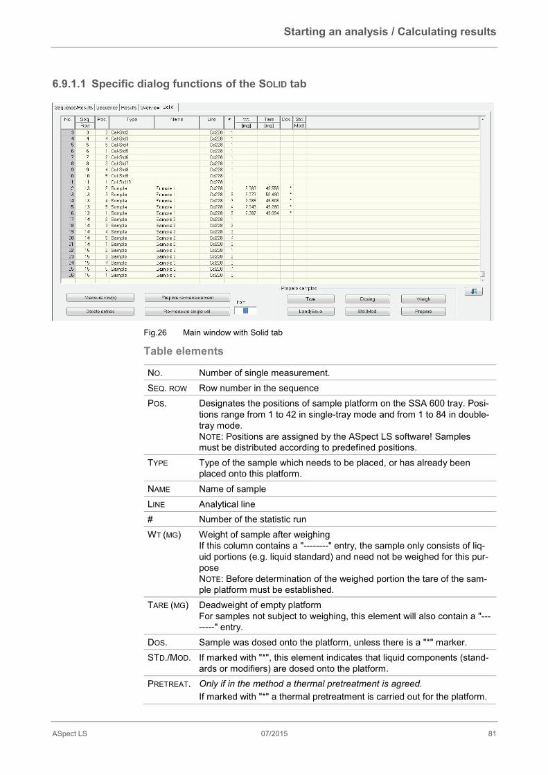
Starting an analysis / Calculating results
ASpect LS 07/2015 81
6.9.1.1 Specific dialog functions of the SOLID tab
Fig.26 Main window with Solid tab
Table elements
NO. Number of single measurement. SEQ. ROW Row number in the sequence POS. Designates the positions of sample platform on the SSA 600 tray. Posi-
tions range from 1 to 42 in single-tray mode and from 1 to 84 in double-tray mode. NOTE: Positions are assigned by the ASpect LS software! Samples must be distributed according to predefined positions.
TYPE Type of the sample which needs to be placed, or has already been placed onto this platform.
NAME Name of sample LINE Analytical line # Number of the statistic run WT (MG) Weight of sample after weighing
If this column contains a "--------" entry, the sample only consists of liq-uid portions (e.g. liquid standard) and need not be weighed for this pur-pose NOTE: Before determination of the weighed portion the tare of the sam-ple platform must be established.
TARE (MG) Deadweight of empty platform For samples not subject to weighing, this element will also contain a "--------" entry.
DOS. Sample was dosed onto the platform, unless there is a "*" marker. STD./MOD. If marked with "*", this element indicates that liquid components (stand-
ards or modifiers) are dosed onto the platform. PRETREAT. Only if in the method a thermal pretreatment is agreed.
If marked with "*" a thermal pretreatment is carried out for the platform.

Starting an analysis / Calculating results
82 07/2015 ASpect LS
If known, the following settings can be directly entered at the sample table:
• Weighed portion if sample preparation occurred on external scales
• Deadweight (tare)
• Marking for completely dosed sample platform
• Marking for completely dosed sample platform, added modifiers and complet-ed thermal pre-treatment
Buttons for sample preparation
[TARE] Determines the weight of an empty platform for marked tray positions. This is accomplished by transferring the respective position contents onto the scales and returning them onto their positions after weighing. The resulting deadweight value will be entered at the TARE column.
[DOSING] Transfers the platforms of marked positions successively into dosing position. A dialog window appears with details regarding the sample that needs to be dosed. Depending on what options were selected, more prepara-tions can be made before or after this sample for marked positions. If a table already contains entries, related preparations will be skipped. Compliance with this order: Tare - Dosing - Weighing - (Dosing) - (Weighing) - Mod./Std Pipetting is compulsory. WITH TARE Weight of empty platform is determined in advance WITH WEIGHING
Dosed sample is weighed after dosing WITH MOD./STD. PIPETTING
Platform is transferred to liquid dosing after weighing. If option WEIGH WITH CONFIRMATION (→ "Autosampler for graphite tube technique (solid analysis)" pg. 37) was configured in the METHOD / SAMPLE TRANSPORT window, "Dosing" and "Weigh" may be repeated for any number of times. If all three options were set, this sequence may be used to run a com-plete sample preparation procedure. On completion of this sequence, the tray will contain filled platforms that are completely prepared for analysis. If one of the preparatory steps was not carried out, this step will be requested as part of the analytical procedure.
[WEIGH] Weigh dosed platform [LOAD / SAVE]
Save and reload weighing and dosing data of selected table rows. The sample table (tab SOLID) is automatically recreated when modify-ing a sequence or method. The existing entries will be lost. Using the function [LOAD/SAVE] these data can be saved and restored.
[STD./MOD.] Only for SSA 600 without liquid dosing Successively transfers the platforms of marked positions into the posi-tion for dosing of liquid analytical constituents (liquid standards, modi-fiers). Displays a dosing screen for liquid dosing. This screen shows the liq-uids to be dosed and the volumes to be dosed.
[PREPARE] Burn-out the platforms for the highlighted positions. The platforms are transferred to the furnace. After running the burn-out program and cooling down, the platforms are then transferred back to the tray. For thermal pre-treatment the modifiers are pipetted to the platform.

Starting an analysis / Calculating results
ASpect LS 07/2015 83
After this the furnace program runs until the step "E/P"is reached. After cooling down the platforms are transferred back to the tray. If the option "WITH TARE" is selected, the platforms are weighted and the weight is displayed in column TARE.
Re-analyze sample / modify weight entries
[MEASURE ROW(S)] Newly determine an element in a sample or measure a se-quence individually in the method development (→ "Re-analyze samples for solid analysis" pg. 85). NOTE: For row measurement of the sample sequence the start must always occur with statistic run 1 or the following run of the last measured statistic run.
[PREPARE RE-MEASUREMENT]
Creates the current SOLID-tab of the statistic run to be remeas-ured from the entries for remeasuring marked in the results ta-ble. After this these sample platforms can be correspondingly dosed and weighed.
[RE-MEASURE SIN-GLE VAL.]
Start measurement of the samples selected with [PREPARE RE-MEASUREMENT].
[DELETE ENTRIES] For selected table rows all entries in columns starting with col-umn WT. [MG] are deleted.
6.9.1.2 Measure solid samples Manual solid analysis If the samples are placed in the graphite tubes with the help of the manual au-tosampler SSA 6 (z), the weighed portion must be determined on a separate scale. The weighed portions are to be entered directly on the SOLID-tab in this case.
Automatic solid analysis for samples that are not time-critical Numerous preparation steps can be combined for samples that are not time-critical. The preparation of samples that are not time-critical is indicated by deactivating the option SEQUENCE FOR TIME-CRITICAL SAMPLES in the window METHOD / SAMPLE TRANSPORT (→ "Autosampler for graphite tube technique (solid analysis)" p. 37).
When using an SSA 600 with liquid dosing unit the pipetting of modifiers and stand-ards is automatically performed during the sequence. Up to four standards and three modifiers can be placed on the SSA 600. If more standards or modifiers are needed these may be pipetted manually. With thermal pretreatment, the modifiers are auto-matically mounted on the platforms through using the liquid dosing unit and then pre-pared for analysis in the graphite tube furnace.
An automatic analysis without intervention of the user requires a sample platform for every individual measurement:
Total number of sample platforms = number of analytical samples x number of analyti-cal lines x number of sample measurements in a statistical series
If the number of samples exceeds the number of platforms defined in the method then the platforms are re-used after analysis.
1. Create a new method and a sequence.
Starting an analysis / Calculating results
84 07/2015 ASpect LS
2. Switch to the SOLID tab in the main window.
3. The column POS. shows the assignment of the samples to the sampler trays. The assignment is determined by the software and cannot be changed.
4. Start processing the sequence by clicking on .
5. Prepare the sample platforms in accordance with the program instructions. Mount the samples and pipette the liquid components if necessary.
6. The measurements starts when all samples are prepared and/or the number of sample platforms configured in the method are mounted.
7. If there are still samples after the first measurement cycle, mark the correspond-ing sample rows in the sequence using the mouse. You can make multiple marks by pressing and holding the shift and/or ctrl buttons.
8. Continue the measurement with and append the results to the existing ones by activating the option APPEND TO FILE/LIST in the window START MEASUREMENT SEQUENCE.
9. Prepare the sample platforms again in accordance with the program instructions. The measurement will then start automatically.
10. Continue with step (6) until all samples have been processed.
Automatic solid analysis for time-critical samples Samples that easily volatize or "creep" due to high adhesion on the platform and soak the edge and handle of the platform require that the platform be processed quickly after the application of the sample. The preparation of samples is conducted by acti-vating the option SEQUENCE FOR TIME-CRITICAL SAMPLES in the window METHOD / SAM-PLE TRANSPORT, see section "Autosampler for graphite tube technique (solid analysis)" p. 37).
1. Create a new method and a sequence.
2. Start processing the sequence by clicking on .
3. Follow further instructions for sample preparation on the monitor screen. A sam-ple will be prepared and measured. The request for the preparation of the next sample platform will follow until all samples have been processed.
The measurement run for time-critical samples requires the constant presence of the user.
6.9.2 Save data of previously prepared samples When the sequence or method is modified the solid table is reconfigured and the samples are reassigned to the platforms. In order to prevent loss of existing weight data these data can be saved. These data can be stored to prevent this. Two storage areas for linked blocks are available for this purpose.
1. Mark the samples which have already been prepared. The data has to be in one contiguous block.
2. Use button [LOAD/SAVE] for opening the window LOAD/SAVE SSA600 TRAY.

Starting an analysis / Calculating results
ASpect LS 07/2015 85
Fig. 27 Window for saving and loading the entries of the solid table
3. Select one of the two MEMORIES.
4. Select [SAVE SELECTED ENTRIES] and confirm the message box with [OK].
5. Quit window LOAD/SAVE SSA600 TABLE with [CLOSE].
6. Reopen the window LOAD/SAVE SSA600 TRAY after the sample table in window SOLID has been rebuilt.
7. Select the MEMORY.
8. Enter the row number of the SOLID table in the list field, from which the data block will be inserted.
9. [LOAD ENTRIES FROM ROW] and confirm the message box with [CLOSE].
10. Quit window LOAD/SAVE SSA600 TRAY by using [CLOSE]. The data block is inserted into the SOLID table starting with the defined table row.
11. Where appropriate re-sort the platforms on the sample tray.
6.9.3 Re-analyze samples for solid analysis Individual samples as well as individual elements can be re-analyzed when using solid analysis technique.
Re-analyze a sample 1. In the main window change to the RESULTS-table.
2. Double-click on the sample. The window SINGLE VALUES is opened.
3. Mark the outlier in the table.
4. Click on [MARK FOR RE-MEASUREMENT].
5. Close the window SAMPLE SINGLE VALUES.
6. In the same way mark all additional outliers of other samples.
7. Return to SOLID-table.
8. Click on [PREPARE RE-MEASUREMENT].
The SOLID-table is created.

Starting an analysis / Calculating results
86 07/2015 ASpect LS
Note
Here the individual values and other entries present are deleted where appropriate as the table is newly structured. If necessary the data should be saved beforehand (→ "Save data of previously prepared samples" pg. 84).
1. Prepare the samples in accordance with the platform assignment for the analysis.
2. Start the measurement with [RE-MEASURE SINGLE VAL.]. The recalculated results for the re-analyzed samples are added to the results ta-ble in window RESULTS.
Re-analyze an element in a sample 1. Mark all single measurements of the sample element in the SOLID-table.
2. Select [MEASURE ROW(S)].
3. Enter a new results file name in window START SEQUENCE or append the data to the existing file.
4. Start measurement with [OK].
Measure the solid table by row (method processing) In the method processing the SOLID-table can be processed by row.
1. Mark the single measurements of the sample element in the SOLID-table.
2. Select [MEASURE ROW(S)].
3. Enter a new results file name in window START SEQUENCE or append the data to the existing file.
4. Start measurement with [OK].
Note
The measurement of an element of a sample must be started with Run #1 or the run which follows the last measured statistics run.
Calibration
ASpect LS 07/2015 87
7 Calibration Calibration is carried out during sample measurement according to the options select-ed in the sequence. The calibration curves and functions can be viewed and edited after the measurement.
Open the CALIBRATION window using menu command METHOD DEVELOPMENT
CALIBRATION...or the icon button .
The CALIBRATION WINDOW displays the calculated calibration curve (taking the curve parameters into account).
Fig. 28 CALIBRATION window
The window contains
• graph of the calibration curve,
• Calibration table
• Parameters
• Residuals
• Limits of detection (LOD) and limits of quantitation (LOQ).
Selection list boxes in Calibration window
LINE Select the element line the calibration of which shall be dis-played.
CALIBRATION FUNCTION
Display of the used calibration function (set in the METHOD / CAL-IB. window). The calibration function is specific for every element line. You may select a new calibration function from the list box. The calibration will then be recalculated accordingly.
METHOD DEVELOP-
MENT CALIBRA-
TION...
Calibration
88 07/2015 ASpect LS
7.1 Graphic presentation of calibration curve In the graph, the measuring points, the calculated calibration curve, and the residuals are displayed. The numbers at the measuring points correspond to those used on the TABLE tab.
Other markings used
Z Zero. Calibration zero Colors of measuring points:
BLACK Normal measuring point LIGHT GRAY Deleted/outlier (not included in calculation) BLUE Suspected outlier (included in calculation)
Curve colors:
BLACK Calibration curve within the valid calibration range BLUE Calibration curve outside the valid calibration range GREEN Lower and upper limit of the prognosis range within the valid calibration
range LIGHT GRAY
Lower and upper limit of the prognosis range outside the valid calibra-tion range
Note on prognosis range
The position of the prognosis range depends on the selected statistical certainty. It is a measure of the "quality” of the calibration, from which also the statistical certainty of the measurement of the analytical samples depends in the end. Besides, the progno-sis range serves to identify suspected outliers among the calibration points. The confi-dence level is to be chosen in the METHOD / STATISTICS window (→ "Enter statistic parameters -STATISTICS tab" pg. 47)
Special case: solid analytics in additive calibration mode An additional PREPARE ADDITION checkbox is displayed in the CALIBRATION window. Measured extinction values will be shown versus the respective sample mass if this box is active. For each addition standard of equal additive volume, a best fitting straight line will be calculated and represented in color. The mean sample mass ap-pears as a vertical inserted line. The points of intersection of the various best fitting lines with this vertical line then provide the basis for calculation of a straight addition line.
7.2 Displaying calibration results Display of measured values of calibration standards – Table tab On the TABLE tab, the value pairs of the standards (entered concentration / measured value) are displayed.
Calibration
ASpect LS 07/2015 89
If the standards were measured repeatedly and a statistical analysis option set in the method, you may additionally activate the display of the standard deviation (SD), the relative standard deviation (RSD%), the range (R) and the relative range (RR%) by selecting the corresponding check boxes.
To exclude individual calibration standards from the calculation, select the standard in the table by a mouse click and then click on [DELETE STD.]. The measurement is only marked as deleted and can be reactivated at any time.
The measurement is only marked as deleted and can be reactivated at any time.
Display of calibration data – Parameters tab This tab shows the calibration data as far as their calculation makes sense.
R² (ADJ.) Coefficient of determination SLOPE Slope of calibration curve METHODSD Standard deviation of the method CHAR. CONC. / CHAR. WEIGHT
Characteristic concentration or weight (concentration or weight required to absorb 1% of the available light energy in the atomizer – corresponding to an absorbance value of approx. 0.0044)
Residuals tab The graph on the RESIDUALS tab shows the deviations of the calibration points from the calculated calibration curve and the limits of the prognosis range.
Limits of detection and quantitation of the current calibration - LOD/LOQ tab The limits of detection and the limits of quantitation of the AAS can be determined based on the current calibration results.
In this area, values of the blank method and the calibration curve method will be dis-played only if the AAS has been calibrated already.
LIMIT OF DETECTION The weight (concentration) of the element to be analyzed that can be detected with a defined statistical certainty.
LIMIT OF QUANTITATION The minimum weight (concentration) of the element to be analyzed that can be determined with a defined confidence level.
SD BLANK Only with blank method. Measured standard deviation of the blank (IDL sample).
[CALCULATE] Starts the calculation of the limits of detection and quantita-tion, e.g. after a change of the calibration curve.
Calibration curve method The calculation of the limits of detection and determination according to the calibration curve method necessitates a linear calibration curve. The calibration should be carried out in the lower concentration range. Calibration parameters that are essential for the result of computation include the following:
• Number and position of calibration points
• Number of repeat measurements per standard
Calibration
90 07/2015 ASpect LS
• Quality of regression
• Slope of calibration curve
• Relative statistical certainty (probability level)
The values obtained from the calibration curve method can be considered useful only if the calibration was run in the lower concentration range.
Blank method The standard deviation of the blank is determined within the sample measurement. For this purpose, the measurement of the blank (QC BLANK DL) is included in the se-quence (→ "Combine sample and action sequences for a sequence" pg. 59).
Calculation instructions for the blank method:
The blank is to be measured 11 x. From the obtained values, the absolute standard deviation SD of the blank is determined. The following formulas apply to the limits of detection and determination:
Limit of Detection (LOD) LOD = 3 * SD / (slope of calibration curve)
Limit of quantitation (LOQ) LOQ = 10.0 * SD / (slope of calibration curve)
7.3 Modifying the calibration curve You can modify an existing calibration curve by the
• change of the used calibration function
• deactivation or activation of standards.
To change the calibration function, choose a new model from the CALIBRATION FUNC-TION list box.
To exclude a standard from the calculation, mark it on the TABLE tab and then click on the [DELETE STD.] button. The measurement is only marked as deleted and can be reactivated at any time.
The program recalculates the calibration curve and displays the modified curve.
The modified calibration parameters will be applied to the results, if you activate menu
command ROUTINE REPROCESS... or click on on the toolbar (→ "Reprocessing analysis results" pg. 70).
ROUTINE REPRO-
CESS

Quality control
ASpect LS 07/2015 91
8 Quality control The Quality Control function serves to monitor the measurement results of a method over a longer period of time. For this purpose, specific QC samples of different types are chosen for a method and included in the measurement series. When evaluating the QC samples, the results are compared to those obtained with previous QC sam-ples.
The evaluations are presented on quality control charts (QC charts) and saved along with the method. The QC charts are available after every loading of the method and will be updated at the next measurement start.
Select the type of QC samples and their parameters in the METHOD window on the QCS tab (→ "Specify quality control samples for QC tabs - QCS tab"S . 49). In the SEQUENCE window, define the integration of the QC samples within the measurement series (→ "Combine sample and action sequences for a sequence", pg. 59).
You can view the QC charts of the loaded (active) method in the QC window. There, you can also define the parameters and the configuration of the QC charts.
Open the QC window using menu command METHOD DEVELOPMENT QC... or
icon button .
8.1 Parameters of QC charts
Fig.29 QC / QC CHART PARAMETERS window
The content of the QC CHARTS is defined in the QC window on the QC CHARTS PARAM-ETERS tab and can be customized to the requirements of your laboratory regarding the frequency of the entries.
METHOD DEVELOP-
MENT QC...
QC CHART PARAME-
TERS

Quality control
92 07/2015 ASpect LS
Joint administrative settings
NUMBER PREP. PE-RIOD
The preparation period is a number of QC chart entries that are used for the calculation of control limits (C) and error limits (E). The preparation period always contains the older chart entries. If set to 0 (no prep. period), all entered QC data will be included in the calculation of control and error limits.
ELIMINATE OUTLIERS (+/- 3S)
Remove values from the previous period which deviate more than 3 Sigma from the ideal value.
MIN. NUMBER OF VALID VALUES
Numbers of values which must at least be contained in the previous period when ELIMINATE OUTLIERS (+/- 3S) is activated.
MAX. NUMBER OF ENTRIES
Total number of entries on a QC chart. A full chart must be renewed (see below).
ENTER SCHEME ALL VALUES Enter every performed QC action. 1 VALUE / DAY Enters the last QC action of the day only. 2 VALUES / DAY Enters the first and the last QC action of the day only.
DEFINITION OF "DAY": A "day" corresponds to one day according to the PC clock, i.e. in the course of a day, any previous entry on the QC chart will be overwritten by a new QC value; however, when a new day begins, a new entry will be generated.
Chart display Specification of the type of QC evaluation to be displayed on the QC chart:
QC sample type Type of QC evaluation QC SAMPLE QC Standard
Mean values MEAN VALUES (NORMALIZED) RECOVERY RATES
QC TREND QC Matrix
TRENDS Ranges Precisions
BLANK No choice. The absorbance of the blank is displayed. Updating displayed charts Defines how to proceed with (almost) full charts:
ACCEPT PREP. PERIOD, DELETE REMAIN
Accepts the preparation period of the old chart for application to the new chart and deletes remaining values.
LAST VALUES > NEW PREP. PERI-OD
The values of the old chart measured last represent the prepara-tion period of the new chart; all other values will be deleted from the chart. New measured values will be evaluated based on the newly created preparation period.
DELETE ALL, NEW PREP. PERIOD
All values will be deleted. New measured values will first fill the preparation period.
[PROCESS] Deletes the charts according to the option selected above.

Quality control
ASpect LS 07/2015 93
Graphic setting In this field, you can choose the point size used for the graph, and if the points shall be connected with each other by a line.
POINT SIZE The individual points are displayed as circles. Choose a higher point size for larger circles.
CONNECT POINTS
Connects the points on the graph with each other by a line.
8.2 Displaying QC charts The QC charts are displayed in the QC – QC CHARTS window.
Separate charts are generated each for every QC sample type defined in the method and for every element line specified there.
Fig.30 QC / QC CHART window
TYPE Here, choose the QC sample type to be displayed. LINE Here, choose the element line to be displayed. DISPLAYED VAL-UES
Number of displayed values and the date of the first and the last value displayed.
ENTRIES Total number of entries on the current QC chart and the date of the first and the last value.
X(MAX) Select the number of entries to be displayed on the graph.
Prints the QC graph inclusive of alphanumerical data and meas-ured values.
Marks and colors used in the QC chart graph
YELLOW FIELD Preparation period
QC CHARTS TAB
Quality control
94 07/2015 ASpect LS
LIGHT GRAY HORIZON-TAL LINE
Mean value calculated from preparation period
RED HORIZONTAL LINES Upper and lower control limit (C) calculated from prepara-tion period (3 Sigma)
GREEN HORIZONTAL LINES
Calculated warning limits (W; 2 Sigma).
SMALL BLACK CIRCLES Measuring points If you click on a measured value on the graph, a window is opened with the following information on this measured value.
NUMBER Number of the measured value in the QC series VALUE Measured value (converted according to the presentation type of the QC
chart) DATE / TIME
Date and time of measurement
USER Displayed when working with User Management indicating the user logged in at the time of measurement.
Controlling and monitoring spectrometer and accessories
ASpect LS 07/2015 95
9 Controlling and monitoring spectrometer and accessories
9.1 Spectrometer
Selected technique: All techniques The SPECTROMETER window serves to test spectrometer functions and method devel-opment. The following data can be adjusted or viewed and the following actions per-formed:
• Checking the lamps
• Stocking of the lamp turret
• Start up behavior of lamps and D2E-lamp
• Lamp spectrum
• Optimization of the ZEEman magnetic field
Activate the SPECTROMETER window using menu command METHOD DEVELOP-
MENT SPECTROMETER... or icon button .
All specification and optimizations occur for the optical parameters set in the window Spectrometer Control, especially for the element line selected there.
9.1.1 Set Optical Parameters – CONTROL tab Set the optical parameters of the spectrometer on the tab CONTROL:
• Wavelength (Elementlinie)
• Slit width
• Lamp current
• Type of background correction
• Optical mode
• Possibly pre-heated lamp
METHOD DEVELOP-
MENT SPECTROME-
TER...
CONTROL TAB
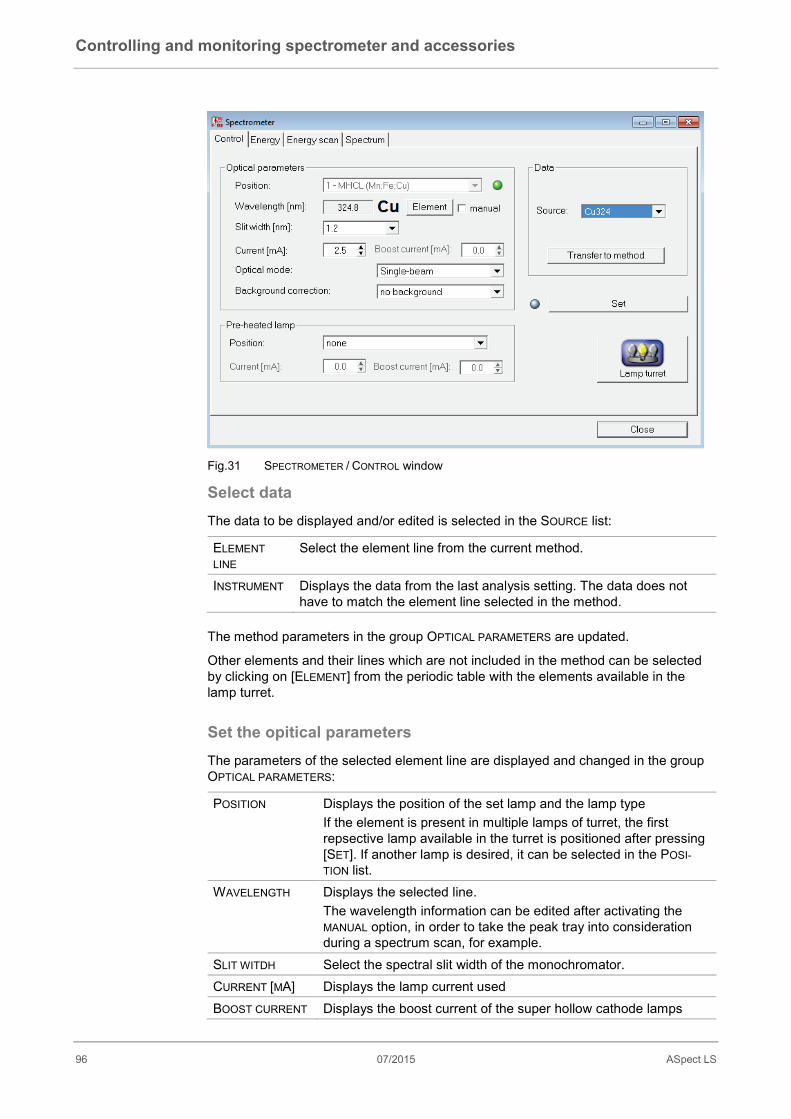
Controlling and monitoring spectrometer and accessories
96 07/2015 ASpect LS
Fig.31 SPECTROMETER / CONTROL window
Select data The data to be displayed and/or edited is selected in the SOURCE list:
ELEMENT LINE
Select the element line from the current method.
INSTRUMENT Displays the data from the last analysis setting. The data does not have to match the element line selected in the method.
The method parameters in the group OPTICAL PARAMETERS are updated.
Other elements and their lines which are not included in the method can be selected by clicking on [ELEMENT] from the periodic table with the elements available in the lamp turret.
Set the opitical parameters The parameters of the selected element line are displayed and changed in the group OPTICAL PARAMETERS:
POSITION Displays the position of the set lamp and the lamp type If the element is present in multiple lamps of turret, the first repsective lamp available in the turret is positioned after pressing [SET]. If another lamp is desired, it can be selected in the POSI-TION list.
WAVELENGTH Displays the selected line. The wavelength information can be edited after activating the MANUAL option, in order to take the peak tray into consideration during a spectrum scan, for example.
SLIT WITDH Select the spectral slit width of the monochromator. CURRENT [MA] Displays the lamp current used BOOST CURRENT Displays the boost current of the super hollow cathode lamps
Controlling and monitoring spectrometer and accessories
ASpect LS 07/2015 97
[MA] OPTICAL MODE Selection of the operating mode: Single beam, double beam or
emission mode BACKGROUND CORRECTION
Selection of the background correction
By clicking on [SET], the selected line as well as the optical parameter are set. The lamp turret will be moved to the required position and the spectrometer will be set to the wavelength. In doing so, a peak search and an auto zero will be conducted. If both are conducted correctly, the control lamp will turn green, otherwise it will turn red.
With [TRANSFER TO METHOD], you transfer the edited data to the method. We recom-mend saving the changed method.
Pre-heated lamp For the method processing a further lamp can be pre-heated in order to shorten the waiting times which are linked with the start up behavior of the lamps.
POSITION Set the lamp position of the lamp to be pre-heated. CURRENT [MA] Lamp current of the lamp BOOST CURRENT [MA] Boost current if a super hollow cathode lamp is pre-heated.
This setting is also realized by clicking on [SET].
[Lamp turret] button Opens the LAMP TURRET window for mounting the lamp turrent (→ "Lamp turret, mounting" pg. 13).

Controlling and monitoring spectrometer and accessories
98 07/2015 ASpect LS
9.1.2 Check lamp energy - ENERGY tab In the window SPECTROMETER / ENERGY the check and control of the lamp energy oc-curs for the optical parameters set on the tab CONTROL.
Fig. 32 SPECTROMETER / ENERGY window
Energy levels
HCL Current energy level of the line radiator at the photo multiplier in % nu-merical and graphic. In addition to the blue current level the graph also shows the gray measured maximum level (i.e. the highest value attained by adjustment). Display for HCL, S-HCL and emission signal.
D2HCL Current energy level of the background radiator D2HCL The current level is shown graphically with a red bar.
[START] Start measurement (e.g. for lamp adjustment). [DELETE] Delete measurement values. [STOP] Stop measurement.
Parameters
PMT [V] Current voltage of the receiver (photomultiplier) in volts value range: max. 600 V
D2HCL-CURRENT [MA] Average lamp current of the deuterium hollow cathode lamp value range: 5 – 35 mA
The energy adaptation between the HCL lamp and the background radiator D2HCL occurs via two separated amplifier settings here.
HC AMPL. LEVEL
Amplification stage between 0 and 4 which only affects the signal of the line radiator.
BC AMPL. LEVEL
This gain stage affects the signal of the background radiator, range 0 to 4, exclusively.
ENERGY TAB

Controlling and monitoring spectrometer and accessories
ASpect LS 07/2015 99
[AGC] Voltage of the photomultiplier and the D2HCL current, equalized to a 65 to 75% energy level (→ "Equalize the energy at the receiver (photomultiplier)" pg. 99.
[PEAK PICK...] Determine actual line maximum of the set spectral line and its devia-tion from the table value (offset). The windowPEAK SEARCH appears in which the offset is shown graphically and numerically. The device wavelengths are corrected according to the established line maximum and a device autozero is executed.
[TRANSFER TO METHOD]
Transfer parameterst o method.
9.1.2.1 Equalize the energy at the receiver (photomultiplier) Proceed as follows to equalize the measured energy:
1. Only in emission mode: Aspirate the solution with the highest expected concen-tration, from the element to be measured, from AAS and allow to be nebulized.
2. Click on [AGC].
3. The voltage of the photomultiplier is automatically set in such a way that the sig-nal of line radiator lies between 65 and 75%.
4. If you are working with background correction the current of the D2HCL is then set such that its signal also lies between 65 and 75%.
5. If automatic equalization to measurement values between 65 and 75% is not successful, manually change the following parameters:
• BC-gain stage
• HC gain stage
• Slit width
• Line radiator current
Click again on [AGC].
If the intensities of both radiators are equalized, all displays are updated.
9.1.2.2 Adjust D2-HCL The adjustment of the D2-HCL occurs in the window SPECTROMETER / ENERGY.
1. In the window SPECTROMETER / CONTROL select the option ONLY D2HCL-BACKGROUND in the selection list BACKGROUNDCORRECTION and start the spec-trometer parameters with [SET].
2. Go to the ENERGY tab.
3. With the [AGC] button, equalize the voltage for the photomultiplier PMT and the D2HCL current with the aim of setting the energy level to 65 to 75% .
4. With the [START] button, begin the energy measurement
5. Set the energy level (red bar) to a maximum value: Note: The gray highlighted bars indicate the last maximum to have been reached and can be deleted with the button [Delete].

Controlling and monitoring spectrometer and accessories
100 07/2015 ASpect LS
• With focus adjusting: Move the lamp holder slightly by hand in the axial direc-tion, then tighten the locking screws.
• With axis adjusting: Adjust fine adjustment screws on the D2-HCL (see hard-ware part of the operating instructions).
6. Proceed, depending on possible error messages or the D2 current:
• If an error message indicates too little energy for the D2-HCL first check the D2 current. If it is not at 35 mA after the control, enter the value 35 mA and repeat the control using the [AGC] button.
• If the D2 current is already at 35 mA, increase the BC amplification by one step (steps from 0 to 4) and repeat the control using the [AGC] button.
• If an error message indicates too much energy for the D2-HCL (too little ener-gy for the HCL), increase the HC amplification by one step (steps from 0 to 4) and repeat the control using the [AGC] button.
The adjustment of the line radiator (hollow cathode lamps) occurs as described in section "Lamp turret, mounting" pg. 13.
Note
The line sources (HCL) are automatically aligned when using the [ALIGN] button in the [LAMP ALIGNMENT]subarea.
9.1.3 Examine lamp drift - ENERGY SCAN tab In the window SPECTROMETER / ENERGY-SCAN the drift behavior of the active lamp and the deuterium lamp, if it was specified for the background correction, are shown graphically and evaluated.
The red line marks the energy flow of the D2-HCL and the blue line marks the energy flow of the active lamp. The signal colors can be freely defined in window OPTIONS – VIEW (→ "View options" p. 154).
For the assessment of the lift behavior the following parameters are displayed:
INTS. [%] intensity of the lamp radiation for HCL and D2-HCL DRIFT [%INTS./MIN]
Ratio of the mean value of 10 values a minute ago and the mean value of 10 values at the current point in time
RANGE Difference of the largest and smallest measurement value in the last minute

Controlling and monitoring spectrometer and accessories
ASpect LS 07/2015 101
Fig.33 SPECTROMETER / ENERGY SCAN window
9.1.4 Take up lamp spectrum - SPECTRUM tab The window SPECTROMETER / SPECTRUM allows the spectrum take up and the presen-tation of all bands in the selected wavelength range for the optical parameters set on the card CONTROL( “Set Optical Parameters – CONTROL tab” pg. 95)..
Fig.34 SPECTROMETER / SPECTRUM window
Unter PARAMETERS legen Sie die Einstellungen für den Spektren-Scan fest:
SPECTRUM TAB
Controlling and monitoring spectrometer and accessories
102 07/2015 ASpect LS
START [NM]
Start wavelength of the spectral range to be taken up
END [NM] End wavelength of the spectral range SPEED Scan speed of the monochromator: SLOW, MEDIUM or FAST. With the
speed SLOW the best signal-noise ratio is attained through the longer in-tegration times.
SIGNALS Selection of the displayed lamp spectra (Can only be selected for D2-HCL-background correction if the D2HCL is switched on). HCL Only signal of the active D2-HCL D2HCL Only signal of the deuterium hollow cathode lamp BOTH Signals of the active HCL and D2-HCL
The spectra scan is started with the buttons.
[START] / [STOP]
[START] deletes the current display and starts the measurement. The button changes to [STOP] with which the measurement can be inter-rupted.
[CONTINUE] Continue interrupted measurement. The result is presented graphically and numerically. The signal colors can be freely defined in window OPTIONS / VIEW (→ "View options" p. 154).
RED LINE Signal of the D2-HCL BLUE LINE Signal of the active HCL GREEN VERTI-CAL
Cursor for the numerical display of wavelength and intensity value The cursor can be moved under the graph with the keys [<] and [>].
HCL Numerical values of wavelength and intensity at the cursor position for the HCL.
D2HCL Numerical values for D2-HCL
9.1.5 Background corrections for ZEEman-AAS
Selected technique: Graphite tube technique with Zeeman-furnace For the ZEEMAN-AAS-APPLIANCES the background correction can be set in the METH-OD - EVALUATION window by means of the Zeeman magnetic field. The following oper-ating modes for the Zeeman magnetic field can thus be selected:
• Zeeman-2-field mode
• Zeeman-3-field mode
• Zeeman Dyn. Mode
The optimum field strengths for the Zeeman-2-field and Zeeman-3-field-modes can be found by means of an optimization program "Optimize ZEEman magnetic field" pg. 103.
The special features of the Zeeman-dynamic-mode are described in the section "The ZEEman dynamic mode" pg. 104.

Controlling and monitoring spectrometer and accessories
ASpect LS 07/2015 103
9.1.5.1 Optimize ZEEman magnetic field For the measurement in the graphite tube technique with background correction in the static 2 field or 3 field modes with a ZEEnit range spectrometer there are optimization programs which automatically pass through a measurement series with different field strengths from a given start to a given end value. The measured values so obtained are output in tabular form, the measurement peaks can be read from the graphs dis-played during the measurement.
With this information determine the optimum field strength for your analysis problem and take this value over into the method. For the optimization, a sample should be used that is as representative as possible of the samples to be analyzed.
The automatic optimization of the field strengths occurs in the window SPECTROMETER – FIELD STRENGTH-OPT.
Parameters for optimizing the 2 field mode In the 2 field mode the maximum field strength is varied during the measurement se-ries.
START [T] Start value for the variation of the maximum field strength (0.01 – 1.00 T) END [T] End value for the variation of the maximum field strength (0.01 – 1.00 T) STEP SIZE Step size for the variation of the maximum field strength (0.05 – 0.25 T)
Parameters for optimizing the 3 field mode In the 3 field mode the medium field strength is varied during the measurement series. The maximum field strength is thus fixed.
START [T] Start value for the variation of the medium field strength (0.05 T)
END [T] End value for the variation of the medium field strength (0.01 – (Max-0.05 T))
STEP WIDTH Step size for the variation of the maximum field strength (0.05 – 0.25 T)
MAX. FIELD STRENGTH
Maximum field strength (0.05 – 1.00 T)
SAMPLER POS. Autosampler position of the sample that is used for the optimi-zation.
Buttons for the optimization
[START] Start measurement series. [TRANSFER TO METHOD] Transfer parameters found into the method. [SAVE] Save results of the optimization. [LOAD] Load saved optimization results.
Display of the optimization parameters The graph shows both absorbance curves for the measurement signal (blue curve) and for the background (red curve). In the selection list it is possible to choose be-tween HEIGHT and AREAof the signal evaluation.
The following values are displayed in the table area:

Controlling and monitoring spectrometer and accessories
104 07/2015 ASpect LS
NO. No. of the optimization step FIELD STR Value for the field strength ABS. HEIGHT (AREA) Absorbance value for the evaluation of the peak height or ar-
ea BACKGR. HEIGHT (AREA)
Background absorbance value for the evaluation of the peak height or area
ZEEMAN-FACTOR Zeeman-Factor (Abs/(Abs. + backgr.))
9.1.5.2 The ZEEman dynamic mode ASpect LS supports a special dynamic mode in the standard calibration method for the spectrometers of the ZEEnit series. This unites the advantages of the stationary 2 field and 3 field Zeeman modes:
• In the lower concentration range, the better sensitivity of the 2-field operating mode can be exploited
• In the upper concentration range, higher concentrations can be measured at the cost of sensitivity in the 3-field mode, in the course of which the well-known Zeeman rollover-effect is shifted to the higher concentrations.
For this, the magnetic field is operated in three states as in the stationary 3-field mode. Only two absorbance values, however, are recorded:
• Absorbance difference between the switched-off magnetic field and the mag-netic field with the maximum field strength (H-value / high sensitivity (high))
• Absorbance difference between the magnetic field of medium field strength and the maximum field strength (L-value / low sensitivity (low))
Both values (L-value and H-value) are recorded and saved in the active integration mode (area or height) at each measurement. The values of the alternative integration mode are not saved, that means that you have to decide on one of the two integration modes before the measurement.
Representation of the H and L values in the tables and graphs The two values are shown in the tables in the same way as in the other Zeeman oper-ating modes of area and height values.
The L-value peak and the H-value peak are shown in the result graphs. The back-ground is depicted for maximum field strength.
The single-peak graph is split into two graphs, one above the other, with different absorbance scales, while all other graphs use a common coordinate system for L and H values.
Calibration of H and L values During the calibration, calibration curves are calculated for the L values and the H values (H curve and L curve).
In the process, it is possible to take calibration points with higher concentrations into account, but only for the L curve. The Button [delete H value] in the calibration table is there for that purpose. Once both calibration curves have been calculated, the user can define a concentration limit.
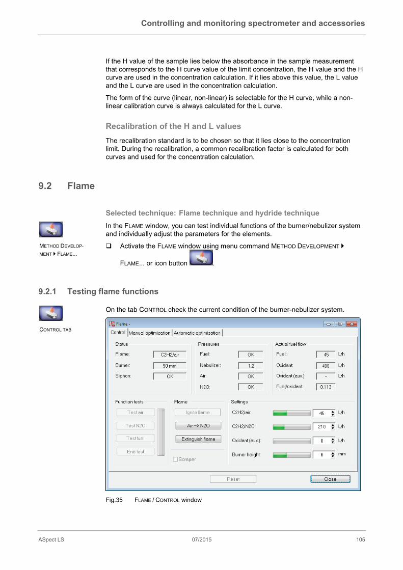
Controlling and monitoring spectrometer and accessories
ASpect LS 07/2015 105
If the H value of the sample lies below the absorbance in the sample measurement that corresponds to the H curve value of the limit concentration, the H value and the H curve are used in the concentration calculation. If it lies above this value, the L value and the L curve are used in the concentration calculation.
The form of the curve (linear, non-linear) is selectable for the H curve, while a non-linear calibration curve is always calculated for the L curve.
Recalibration of the H and L values The recalibration standard is to be chosen so that it lies close to the concentration limit. During the recalibration, a common recalibration factor is calculated for both curves and used for the concentration calculation.
9.2 Flame
Selected technique: Flame technique and hydride technique In the FLAME window, you can test individual functions of the burner/nebulizer system and individually adjust the parameters for the elements.
Activate the FLAME window using menu command METHOD DEVELOPMENT
FLAME... or icon button .
9.2.1 Testing flame functions On the tab CONTROL check the current condition of the burner-nebulizer system.
Fig.35 FLAME / CONTROL window
METHOD DEVELOP-
MENT FLAME...
CONTROL TAB
Controlling and monitoring spectrometer and accessories
106 07/2015 ASpect LS
Status
FLAME Status display of the flame: OFF The flame is not burning. C2H2/AIR The acetylene/air flame is burning. C2H2/NO2 The acetylene/nitrous oxide flame is burning.
BURNER Attached burner head: 100 MM 100-mm single-slot burner 50 mm 50-mm single-slot burner Error No burner head present or is not recognized.
SIPHON The fill level of the siphon (drain trap) below the mixing chamber is moni-tored. OK The siphon is filled with liquid up to the overflow port. Error The fill level of the drain trap is insufficient. The siphon must always be filled sufficiently to prevent backfiring of the flame, particularly that of the nitrous oxide flame.
Pressures
FUEL Status of fuel pressure at device inlet "-" – No fuel pressure detected
NEBULIZER Operating pressure at nebulizer. AIR Status of air inlet pressure. Only displayed if the air supply is open. N2O Status of nitrous-oxide inlet pressure. Displayed only when the nitrous-
oxide supply is open. Current gas flows
FUEL Fuel flow OXIDANT Oxidant flow through nebulizer OXIDANT (AUX.) Auxiliary oxidant
Displayed only if auxiliary oxidant is activated in the method. Air 75 / 150 / 225 NL/h Nitrous oxide (N2O) 60 / 120 / 180 NL/h
FUEL/OXIDANT Fuel/oxidant flow ratio Test functions The test functions are accessible only if the flame is extinguished. The availability of the test functions depends on the context.
[TEST AIR] Opens solenoid valve in air path. REQUIREMENT: Air and fuel are supplied (inlet pressures detected) Displayed parameters: Nebulizer pressure, oxidant flow and total oxidant as long as auxiliary oxidant is activated in the method (→ "Specify flame parameters - FLAME tab" pg. 23).
Controlling and monitoring spectrometer and accessories
ASpect LS 07/2015 107
[TEST N2O] Only for acetylene nitrous oxide flame and 50-mm-one slit burner active Opens solenoid valve in nitrous-oxide path. REQUIREMENT: Nitrous oxide and fuel are supplied (inlet pressures detected). Displayed parameters: Nebulizer pressure, oxidant flow and total oxidant, if auxiliary oxidant was activated..
[TEST FUEL] Adjusts the rated gas flow (proportional valve). Displayed parameters: Fuel flow for acetylene/air flame (for [TEST AIR] or the acetylene/nitrous-oxide flame (for [TEST N2O]). [TEST AIR] or [TEST N2O] must be activated before [TEST FUEL GAS].
[END TEST] Finishes the function test. Flame / Scraper
[IGNITE FLAME] Ignition of the acetylene/air flame: Air supply is released. Ignition arm is swiveled out; the coiled filament is glowing. The rated acetylene flow (proportional valve) is adjusted, when nebulizer pressure and oxidant flow have reached their rated val-ues. Process is aborted, if the flame fails to ignite within 10 seconds. If the flame is burning, the [EXTINGUISH FLAME] button becomes ac-tive. [IGNITE FLAME] is active, if the flame is not burning.
[AIR→N2O] Switching from acetylene/air to acetylene/nitrous-oxide flame: Oxidant valve (3/2 solenoid valve) switches from air to nitrous ox-ide. The fuel flow for the acetylene/nitrous-oxide flame (proportional valve) is adjusted. The button label turns into [N2O→AIR].
[N2O→AIR] Switching from acetylene/nitrous-oxide flame to acetylene/air flame: Oxidant valve (3/2 solenoid valve) switches from nitrous oxide to air. The fuel flow for the acetylene/air flame (proportional valve) is ad-justed. The button label turns into [N2O→AIR].
[EXTINGUISH FLAME]
Extinguishes the flame: If the acetylene/nitrous oxide flame is burning, the system switches to the acetylene/air flame and waits for a few seconds. The fuel flow (proportional valve) is shut off. After a few seconds waiting time (for purging the fuel from mixing chamber and burner), the air supply (solenoid valve) is shut off.
SCRAPER Only with 50-mm single slot burner with mounted scraper and acet-ylene/nitrous-oxide flame. Activates the scraper for cleaning the burner head.
Settings In the SETTINGS field, you may edit the gas flow settings:
C2H2/AIR Acetylene/air flame: (Fuel flow = 40 – 120 NL/h) C2H2/NO2 Acetylene/nitrous-oxide flame (Fuel flow = 120 – 315 NL/h)

Controlling and monitoring spectrometer and accessories
108 07/2015 ASpect LS
OXIDANT (ADDITION) Setting of the auxiliary oxidant flow
BURNER HEIGHT Height of burner relative to optical axis.
Note
The attached burner is automatically detected by the burner sensor. Switching be-tween C2H2/air and C2H2/N2O is possible only if the flame is burning, and if the 50-mm burner has installed.
9.2.2 Optimizing the flame For the analysis, the flame can be optimized for every element line with respect to
• Fuel flow
• Burner height
• Total oxidant flow, if the use of auxiliary oxidant has been chosen in the meth-od.
You may optimize the flame manually by changing the parameters and observing the signal level, or you may have the parameters searched automatically by the applica-tion. In both cases, you may transfer the found parameters to the method at the push of a button.
9.2.2.1 Manual flame optimization Manual flame optimization is carried out in the FLAME / MANUAL OPTIMIZATION window.
Fig.36 FLAME / MANUAL OPTIMIZATION window
MANUAL OPTIMIZA-
TION TAB
Controlling and monitoring spectrometer and accessories
ASpect LS 07/2015 109
LINE Choose the element line for which the flame shall be optimized. You may choose among the analysis lines defined in the method.
[SET] Moves the monochromator to the selected analysis line. FUEL [L/H] Adjustment of fuel flow. BURNER HEIGHT [MM]
Adjustment of burner height relative to the optical axis of the light path of the lamp.
OXIDANT (AUX.) [L/H]
Set auxiliary oxidant flow: Air: 75 / 150 / 225 NL/h N2O: 60 / 120 / 180 NL/h
OXIDANTS [L/H] Display of the oxidant flow in L/h. FUEL/OXIDANT Display of the fuel/oxidant flow ratio. [START] Starts the measurement. The signal is continuously being rec-
orded. The button label turns into [STOP].
[STOP] Stops the measurement. [AZ] Start autozero measurement. [ACCEPT VALUES] Accepts the found flame parameters for the selected element line
and transfers them to the method. GRAPH Display of signal curve.
Ordinate expansion is possible via the input fields at the Y-axis. ABSORBANCE Display of current absorbance value. MAXIMUM Display of the maximum absorbance value of the running meas-
urement. Procedure 1. From the LINE list box, choose the desired element line.
2. Click on [SET] to drive the monochromator to the wavelength of this line.
3. Immerse the tube of the nebulizer into the zero solution.
4. Start the AZ measurement by using the [AZ] button.
5. Immerse the nebulizer sample tube into the sample solution.
6. Start the measurement with [START].
7. Vary the FUEL setting by means of the arrow buttons and watch the signal change in the graph and in the ABSORBANCE field. Adjust the fuel rate until absorbance is maximal.
8. In the same way, adjust the BURNER HEIGHT, until you have found the maximum absorbance.
9. When using the flame with auxiliary oxidant, vary the OXIDANT (AUX.) parameter until again you obtain the maximum signal level.
10. Repeat steps 5 to 7, until you can no longer notice a relevant increase of the signal level.
11. Finish the measurement with [STOP].
12. Click on [ACCEPT] to transfer the found parameters for the selected element line to the method.

Controlling and monitoring spectrometer and accessories
110 07/2015 ASpect LS
In the same way, find the appropriate parameters for all element lines defined in the method.
Note
There is a small delay between the modification of the parameters and the signal re-sponse.
9.2.2.2 Automatic flame optimization Automatic flame optimization is carried out in the FLAME window on the tab AUTOMATIC OPTIMIZATION.
The used optimization algorithm changes the settings for fuel flow and burner height with the aim to obtain an increase in the signal level. This algorithm takes into account the interactions between the two parameters (fuel flow and burner height). The optimi-zation procedure will be stopped if in three successive steps no further increase in signal level is achieved. This means that either the maximum signal level was reached or the change of the parameters is of no effect on the signal level.
Fig. 37 FLAME /AUTOMATIC OPTIMIZATION window
LINE Choose the element line for which the flame shall be optimized. You may choose among the wavelengths defined in the method.
POSITION Position of the test sample on the autosampler. ALL LINES Establish the flame parameters automatically for all element lines in
the method. [START] Starts the measurement. The signal is continuously being recorded.
The button label turns into [STOP]. [STOP] Stops the measurement. [DELETE ] Deletes obtained values.
AUTOMATIC OPTIMI-
ZATION TAB

Controlling and monitoring spectrometer and accessories
ASpect LS 07/2015 111
[LOAD] Loads optimized flame parameters. [SAVE] Saves optimized flame parameters. [ACCEPT VAL-UES]
Accepts the found flame parameters for the selected element line and transfers them to the method.
TABLE Display of found parameters. GRAPH Display of signal curve.
Procedure 1. From the LINE list box, choose the desired element line.
2. Immerse the nebulizer sample tube into the sample solution.
3. Start the optimization using [START]. The dialog window AUTOMATIC OPTIMIZATION is opened.
4. If appropriate, activate following settings:
SET OPTIMIZED VAL-UES AUTOMATICALLY FOR THE CURRENT METHOD
This setting has to be activated for automatic optimization because only the parameters from the last optimization are available after the procedure is completed.
AUTOMATICALLY SAVE OPTIMIZATION DATA
If activated, enter the desired file name in the field FILE NAMES.
5. For single line optimization: If not arranged prior to the optimization, following
successful optimization transfer the parameters for the element line into the method with [ACCEPT].
9.2.3 Extinguishing the flame You may extinguish the flame in different ways.
In the window FLAME-CONTROL extinguish the flame with the button [EXTINGUISH FLAME].
Alternatively, you may activate the menu command ROUTINE EXTINGUISH FLAME.
9.3 Furnace In the window FURNACE the following parameters are set or furnace functions moni-tored:
• Parameters of the furnace programs used in the method
• Selection of modifiers
• Optimization of the atomization and pyrolysis temperatures in the method pro-cessing
• Coating of the graphite tube for the hydrEA technique
• Graphical representation of furnace program
• Check of the furnace functions.
CONTROL TAB
ROUTINE EXTIN-
GUISH FLAME

Controlling and monitoring spectrometer and accessories
112 07/2015 ASpect LS
Use a METHOD DEVELOPMENT / FURNACE... command or click the icon to open the FURNACE window.
Control buttons in Furnace window
LINE A list field for setting an analytical line, for which furnace parameters are to be displayed or varied. Use arrow keys to page through the lines list as necessary.
[→METHOD] Transfers changes in furnace parameter settings for analytical line to "Method".
9.3.1 Editing a furnace program Working in the FURNACE – FURNACE PROGRAM window, a furnace program (tempera-ture-versus-time program (TTP)) can be created, displayed and edited if necessary for a selected analytical line.
A furnace program may comprise a maximum of 20 working steps.
Fig. 38 FURNACE / FURNACE PROGRAM window
Tabular display A tabular display will list all working steps which are part of a currently selected fur-nace program. The parameters on display are:
STEP Sequential number of working step * No function was assigned to this field so far.
NAME Name of furnace program step TEMP. Target temperature in program step RAMP Heating rate in program step
METHOD DEVELOP-
MENT / FURNACE...
FURNACE PROGRAM
TAB

Controlling and monitoring spectrometer and accessories
ASpect LS 07/2015 113
HOLD Holding time of target temperature within program step TIME Total duration of working step GAS Supply internal gas (INT.) and additive gas (ADD.). Possible states:
STOP No supply MIN Minimal supply rate (only internal gas flow) MAX Maximal supply rate
INJ. Injection step. Sample will be injected into furnace on completion of this step.
E/P Working step for enrichment or thermal pretreatment of individual compo-nents.
Control buttons and input fields
[APPEND] Inserts a new line at the end of a list. [INSERT] Inserts a new line before a marked list place. [DELETE ] Delete marked lines. [DELETE TA-BLE]
Deletes entire furnace program table.
MEASURING START DELAY
Allows specification of a time delay for acquisition of measuring sig-nal if required. By default, acquisition of a measuring signal will begin as the ATOM-IZE furnace program step starts. A time setting will delay the starting point of signal acquisition by the preset amount of time. This func-tion is included to allow users to wait with the triggering of a meas-urement until the atomization temperature has actually been reached and remains on a given temperature plateau.
Copies the parameters in a line to all subsequent lines.
[COOKBOOK PROGRAM]
Loads the furnace program for a selected analytical line from the cookbook.
[CHECK PRO-GRAM]
Checks the furnace program. If the furnace program is found to con-tain errors of a kind that renders program execution impossible, the faulty step will be displayed in a message box. The program cannot be launched in this case. Correct the faulty step (or change the fur-nace program that precedes this step). As part of a program start, the furnace will be checked for potential thermic overheat situations (if all basic conditions are known). If the settings for temperature or time are found to be excessively high, a "Thermal furnace overheating”error message will appear during the program startup routine – the furnace program will be abandoned in this case. You should then correct the steps with the highest furnace temperature and the longest holding time.
[TRANSFER DRYING STEP(S)]
For analysis of several lines Accepts and transfers the settings made for drying parameters to the furnace programs for each analytical line.
[TRANSFER CLEANING STEP(S)]
For analysis of several lines Accepts and transfers the settings made for graphite tube baking to the furnace programs of each analytical line.

Controlling and monitoring spectrometer and accessories
114 07/2015 ASpect LS
Specifying parameters for individual furnace program steps On selection of an analytical line, a suitable furnace program will initially be loaded from the cookbook.
Use the [NEW], [INSERT] or [DELETE] control button as necessary to adapt the cur-rent furnace program to your requirements.
To edit, click a desired one of the table cells.
A list will open in this cell if preselections are limited. Numbers must be edited di-rectly in the field.
Program steps:
DRYING Solvent in sample evaporates PYROLYSE Performs thermal pretreatment for decomposition of sample without ad-
ministration of oxygen. ASH Performs thermal pretreatment for thermal decomposition of sample,
using a selectively involved type of additive gas (for example, oxygen supply).
AZ *Zero balancing, measures optical zero state (absorbance = 0) ATOMIZE Sets analytical atoms free. CLEAN Removes residual sample matter.
Temperature settings:
TEMPERATURE End temperature of this step. Value range: Maximal temperature up to 3000°C in steps of 1°C Minimal temperature not less than 20°C above cooling water tem-perature (preferentially 35 °C) of circulation cooler
RAMP The rate of heating intended to achieve target (end) temperature. Value range:1 ... 3000°C/s in steps of 1°C/s; FP (Full Power), NP (No Power) are possible limit rates.
HOLD The time for which a target (end) temperature is to be maintained. Value range: 0 to 999 s less heating time
TIME Total duration of a step (sum of heating time plus hold time), is au-tomatically calculated.
Gas supply
INT. Flow of protective gas. STOP No supply, active 2 s before transition to other step MIN Minimal supply rate (0.1 L/min Ar) MAX Maximal supply rate (2.0 L/min Ar)
ADD. Flow of additive gas, e.g. air, nitrogen, etc. STOP No supply, active 2 s before transition to other step MAX Maximal supply rate (0.5 L/min)
Injection step/thermic pretreatment
INJ. If marked with a "*", the particular sample (gas in HydrEA technique) will not be introduced into the graphite tube before completion of this step (pipetting into preheated tube).

Controlling and monitoring spectrometer and accessories
ASpect LS 07/2015 115
E/P In the case of enrichment, / thermal pre-treatment (Enrichment / Pretreatment) the sample will undergo pretreatment to the point of an enrichment step during a measurement cycle, the tube is then cooled down to room temperature and the next sample volume introduced by pipetting. In the case of thermal pretreatment of analytical solution and/or modifiers, pre-treatment will be performed up to a specified step. At the end of this step the remaining components will be placed into the hot tube. When using thermal pre-treatment with solid technique the furnace program runs until this step is reached. The furnace program for sample measurement is started at this step. The number of desired enrichment cycles, the involvement of modifiers and the type of thermal pretreatment can be specified in the FURNACE – MOD-IF.+Extras window (→ "Matrix modifiers, selections" pg. 115).
9.3.2 Matrix modifiers, selections for enrichment and pretreatment The following parameters are specified in the window FURNACE / MODIF.+EXTRAS:
• Use and volume of matrix modifiers
• Enrichment in the graphite tube through repeated pipetting and drying
• thermal pre-treatment of the sample
Fig.39 FURNACE / MODIF.+EXTRAS window for solution analytics
Selections for modifiers for matrix delimitation and thermal pretreatment must be made for each specific line.
Matrix modifiers Up to five modifiers can be specified for analysis of a given element line. These can be activated by clicking into the relevant modifier checkbox.
In order to prevent errors due to carryover effects, analytical components are recorded in the following standard order:
FURNACE MOD-
IF.+EXTRAS TAB

Controlling and monitoring spectrometer and accessories
116 07/2015 ASpect LS
• Blank (in case of dilution)
• Modifier 1
• ...further modifiers (if specified)
• Sample solution.
Outputs to the graphite tube occur in reverse order, i.e. the sample will be the first to be injected. As the other components are being supplied, residual sample matter will be washed from the dosing tube and injected into the graphite tube. This standard order of sample (first) and modifiers (then) may be modified if necessary.
Required parameter entries for modifiers are:
CHECKBOX Activates modifier for analysis. NAME This list field contains the names of typically used modifiers.
Select a name from this list or enter this name directly at the input field. VOL. Enter discharge volume (1 to 50 µL) here. POS. Specifies position of modifier on sample changer. TO SAMPLE Autosampler will pick the particular modifier up, after the sample was
picked up, i.e. the sample will be injected into the graphite tube before the sample if this box is active.
PRETREAT. Sets thermal pretreatment of modifier. Enrichment For enrichment, a given furnace program is repeatedly performed until the specified step is reached (column E/P). As part of each cycle, the sample quantity which is specified per sample table will be injected and pretreated, the tube is then cooled to room temperature and the next sample volume is injected. This procedure allows greater sample volumes to be placed into the furnace. Modifier volume is injected only once.
Specifiable enrichment modes are:
OFF No enrichment specified. PERMANENT (ON-LY SAMPLES)
Enrichment with each sample (without special samples such as standards, etc.)
PERMANENT (INCL. CALIBRATI-ON)
Enrichtment with each sample, including standards, QC samples and additive standards
IF CONC. TO LOW Enrichment applies only to samples with a concentration level lower than that of the detection limit.
CYCLES Number of enrichment cycles (2 to 100). NOTE: Given that any contaminant present inside the tube will be enriched together with the actual element being analyzed, the number of enrichment steps defined for actual samples should be kept reasonably small.
Thermal pretreatment For thermal pretreatment of analytical solution and/or modifiers, this option will be executed up to the specified working step of a furnace program. At the end of this step, the remaining components will be injected into the preheated tube.

Controlling and monitoring spectrometer and accessories
ASpect LS 07/2015 117
THERMAL PRETREA-TMENT
Performs thermal pretreatment of modifiers or a sample if ac-tive. To define pretreatment of a MODIFIER, the related PRETREAT checkbox must be turned on. NOTE: The modifier pre-treatment temperature may exceed the pyrolysis temperature of the sample.
PREHEAT SAMPLE Pretreats analytical solution, adds modifiers and other compo-nents.
WARM UP DELAY Defines waiting time from addition of components to undergo thermic pretreatment to next components.
Warning! Cool down the tube if thermal pre-treatment exceeds 300 °C!
If the temperature of the thermal pre-treatment exceeds 300 °C, an additional step has to be inserted before adding additional components for cooling down the graphite to temperatures lower than 300°C. When pipetting into the hot graphite tube (>300°C), the cannula may be damaged! No warning is displayed!
Solid analytics with involvement of SSA 600 solid sampler With SOLID ANALYTICS, only matrix modifiers may be specified for addition. Once a modifier has been activated, its name and volume can be defined (same as above).
For SSA 600 WITHOUT LIQUID DOSING the modifiers must be pipetted to the sample by hand. The supply occurs immediately before the platform is brought into the furnace or as the final step of a complete sample preparation with the help of SSA 600.
For SSA 600 WITH LIQUID DOSING, a modifier or liquid samples are automatically pipet-ted.
For thermal pre-treatment in solid analysis the platforms are pre-treated using a modi-fier (e.g. palladium). After this the furnace program runs until the step "E/P"is reached and the coated platform is tared. The furnace program is continued after the sample has been dosed.
9.3.3 Optimizing atomization temperature Working in FURNACE - OPTIMIZATION window, you may perform a series of measure-ments with stepped pattern of increasing settings for step end temperature, in order to determine and set the optimal pyrolese and atomization temperature for a particular element line.
Once optimized, furnace parameter settings for atomization and pyrolese can be saved and loaded to other methods.
OPTIMIZATION TAB
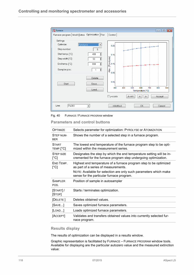
Controlling and monitoring spectrometer and accessories
118 07/2015 ASpect LS
Fig. 40 FURNACE / FURNACE PROGRAM window
Parameters and control buttons
OPTIMIZE Selects parameter for optimization: PYROLYSE or ATOMIZATION STEP NUM-BER
Shows the number of a selected step in a furnace program.
START TEMP.[°C]
The lowest end temperature of the furnace program step to be opti-mized within the measurement series.
STEP SIZE [°C]
Designates the step by which the end temperature setting will be in-cremented for the furnace program step undergoing optimization.
END TEMP. [°C]
Highest end temperature of a furnace program step to be optimized as part of a series of measurements. NOTE: Available for selection are only such parameters which make sense for the particular furnace program.
SAMPLER POS.
Position of sample in autosampler
[START] / [STOP]
Starts / terminates optimization.
[DELETE ] Deletes obtained values. [SAVE...] Saves optimized furnace parameters. [LOAD...] Loads optimized furnace parameters. [ACCEPT] Validates and transfers obtained values into currently selected fur-
nace program. Results display The results of optimization can be displayed in a results window.
Graphic representation is facilitated by FURNACE – FURNACE PROGRAM window tools. Available for displaying are the particular autozero value and the measured extinction value:

Controlling and monitoring spectrometer and accessories
ASpect LS 07/2015 119
RED LINE Background signal that depends on pyrolese or atomization tempera-ture
BLUE LINE Specific absorption depending on pyrolese or atomization temperature VERTICAL CURSOR
User-selected optimal pyrolese or atomization temperature
Y-SCALING If this checkbox was set, y-axis scaling will be such that the back-ground signal can be depicted in the best possible manner. An opti-mized scaling can be separately selected for pyrolese and for atomiza-tion.
[A->H]/[H->A]
Switches the graphic between signal area (Area) and signal height (Height).
[<] / [<] Shifts vertical lines for pyrolese or atomization temperature (depending on what step was selected for optimization) to the left or the right, thus defining a desired optimal furnace temperature.
Performing optimization An autosampler is required to perform this series of measurements.
Optimization goal
PYROLYSE TEMPERATURE: No specific and only minimal non-specific absorption loss.
ATOMIZATION TEMPERA-TURE:
One single consistent specific extinction.
1. Create a method for the current analysis line and save it.
2. Open the window FURNACE and where appropriate adapt the furnace program.
3. Enter optimization settings in the FURNACE / OPTIMIZATION window (optimized temperature, START TEMP.[°C], STEP SIZE[°C], END TEMP. [°C], position of sample on autosampler).
4. Prepare sample on autosampler.
5. Click [START] to trigger optimization.
Optimization will run automatically. Measured results will be displayed in the main window and represented in graph-ical form in the FURNACE / OPTIMIZATION window. To display individual sample readings, click onto a measurement point of the graphic or use a double click onto the sample line in the results window.
6. Use [<] / [>] control buttons to move the vertical cursor over the graphic area or use arrow keys as necessary to adjust optimal temperature. Then click [ACCEPT] to transfer this value into the furnace program.
7. Repeat this procedure for all other analytical lines included in the current method.
9.3.4 Graphical representation of furnace program / graphite tube coating The FURNACE / PLOT window provides the following functions:
• Graphical representation of furnace program
• Monitoring execution of current furnace program
PLOT
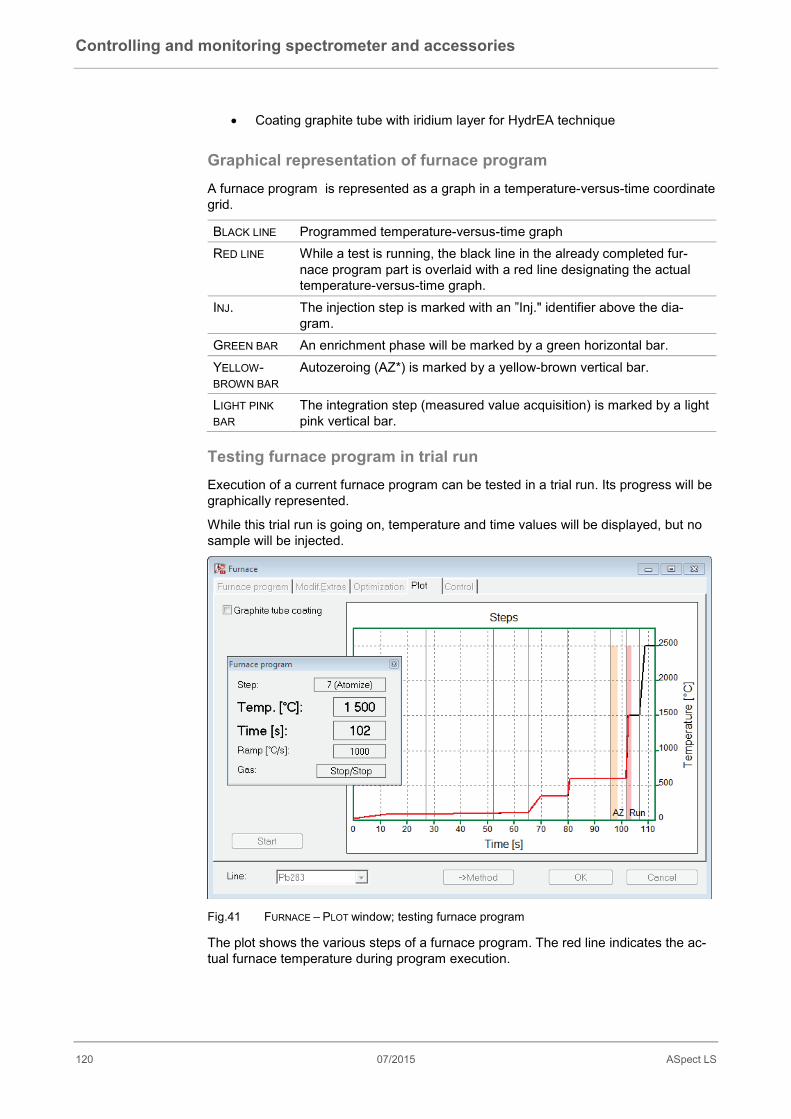
Controlling and monitoring spectrometer and accessories
120 07/2015 ASpect LS
• Coating graphite tube with iridium layer for HydrEA technique
Graphical representation of furnace program A furnace program is represented as a graph in a temperature-versus-time coordinate grid.
BLACK LINE Programmed temperature-versus-time graph RED LINE While a test is running, the black line in the already completed fur-
nace program part is overlaid with a red line designating the actual temperature-versus-time graph.
INJ. The injection step is marked with an ”Inj." identifier above the dia-gram.
GREEN BAR An enrichment phase will be marked by a green horizontal bar. YELLOW-BROWN BAR
Autozeroing (AZ*) is marked by a yellow-brown vertical bar.
LIGHT PINK BAR
The integration step (measured value acquisition) is marked by a light pink vertical bar.
Testing furnace program in trial run Execution of a current furnace program can be tested in a trial run. Its progress will be graphically represented.
While this trial run is going on, temperature and time values will be displayed, but no sample will be injected.
Fig.41 FURNACE – PLOT window; testing furnace program
The plot shows the various steps of a furnace program. The red line indicates the ac-tual furnace temperature during program execution.

Controlling and monitoring spectrometer and accessories
ASpect LS 07/2015 121
During program execution, the following values are output for digital display:
STEP Furnace program step being performed TEMP.[°C] Current furnace temperature TIME [S] Time lapsed since program start RAMP [°C/S] Current heating rate GAS Current gas flow
Graphite tube coating For HydrEA technique, an iridium- or gold-coated graphite tube is required. A coating process can be controlled via the FURNACE - PLOT window.
Once the GRAPHITE TUBE COATING checkbox is marked, the following input parameters will be enabled for selections to run this procedure.
CYCLES Number of enrichment cycles for coating POSITION The sample tray position that contains solution for coating VOL.[µL] Volume of coating solution, which must be pipetted into the tube for each
enrichment step. ELEMENT Selection of the coating material
Use iridium for the analyses of hydrides and gold for the analysis of mer-cury.
[START] Triggers coating.
9.3.5 Further furnace functions Available functions in the FURNACE - CONTROL window are:
• Information relating to the graphite tube
• Formatting graphite tube
• Baking (cleaning) of graphite tube
• Opening / closing of graphite tube
• Indication of current cooling water temperature
• Set up of water cooler
CONTROL TAB

Controlling and monitoring spectrometer and accessories
122 07/2015 ASpect LS
Fig. 42 FURNACE / CONTROL window
Graphite tube data The GRAPHITE TUBE subarea contains information items regarding the graphite tube. This information must be defined when the tube is replaced. It will be automatically updated hereafter. On installation of a new tube, you must set all entries to 0.
TUBE TY-PE
Tube type as per selection in MAIN SETTINGS window
HEAT CYCLES
Number of heating cycles of this tube
LIFETIME Statistical ratio for thermic strain exposure of graphite tube as a product of control parameters and step times of currently active furnace program. This numerical ratio can always be estimated only for a particular type of job.
Note
Before removing a graphite tube which is still in a state fit for operation, you are rec-ommended to record its operating data from the GRAPHITE TUBE subarea in order to be able to restore these values for automatic subsequent updating after the tube has been installed again.
Formatting graphite tube Graphite tube formatting is performed to:
• force air oxygen out of the furnace and adapt the contract pressure force of the moving furnace part,
• recalibrate the furnace temperature,
• format a new installed graphite tube,
Controlling and monitoring spectrometer and accessories
ASpect LS 07/2015 123
• clean the furnace after breaks in operation/idle periods.
Situations where furnace formatting is compulsory:
• after power to the spectrometer is turned on
• after closing a previously open furnace.
FF% Formation factor determined as part of formation [FORMATION] Triggers formation.
The FORMAT TUBE window will appear. It shows currently measured furnace data. Nine temperature stages (300 – 1500 – 300 – 1500 – 300 – 1000 – 1600 – 2000 – 2400 °C) are run and the control temper-atures in the inner tube space are measured. On completion of the last step, the formation factor will appear and the data obtained for tube temperature recalibration will be saved.
Water cooler Configure the water cooler.
AUTO The water cooler is controlled automatically for keeping the cooling water temperature in the working range.
PERMANENT The water cooler runs permanently for maximum cooling capacity. Clean furnace Clean furnace is a single-step cleaning program. It works with a gas rate setting that is fixed to maximum flow. Current parameter settings which can be modified here will be saved with the method.
TEMP [°C] Temperature of baking out (cleaning) RAMP [°C/S]
Heating rate
HOLD [S] The time for which baking lasts [START] Triggers a baking (cleaning) process, displays the Clean furnace window
that reports currently measured furnace date. Further furnace functions
COOLING WATER TEMP. [°C]
Shows current cooling water temperature.
FURNACE LED / FURNACE
Turns the furnace camera on if active. A special window with a graphite tube image will be imposed onto the screen. Sample injection can be monitored. The furnace camera is delivered with permanently On preset-ting. The option to influence this setting is part of the OPTIONS – ANALYSIS SEQUENCE window (→ "Options for analysis se-quence" pg. 157).
[OPEN FURNACE] Opens the graphite tube furnace Graphite tube can be retrieved or installed.
[CLOSE FURNACE] Closes the graphite furnace tube. [RESET FURNACE] Carry out a reset of the furnace computer. [ADJUST ILLUMINA-TION]
Open a window for readjusting the furnace camera illumina-tion.
Controlling and monitoring spectrometer and accessories
124 07/2015 ASpect LS
TEMPERATURE FOR LED SWITCH-OFF
Furnace temperature from which the LED of the illumination unit is switched off. At the same time the furnace camera is switched off and the measurement value acquisition is pre-pared.
Test furnace Checks the furnace for sensor errors. If one of the error states listed here appears, every measurement will be aborted (on the screen a corresponding error message will be displayed).
The error test is started with the [TEST] button. On successful completion of testing, the result will be reported by a green control lamp, on unsuccessful completion by a red control lamp.
9.4 Hydride system
Selected technique Hg/hydride system or HydrEA-system In the HYDRIDE SYSTEM window, you can:
• check the status of the hydride system
• test various functions of the system for errors
• newly initialize the hydride system
• load the system tubes with reagents before the start of analysis
• rinse the system, e.g. after the end of the analysis for cleaning
Open the HYDRIDE SYSTEM window using menu command METHOD DEVELOPMENT HYDRIDE... or the icon button
.
Control buttons in Hydride system window
[INITIALIZE] Initialize the hydride system. [LOAD SYS-TEM]
Load the tubes of the hydride system with reagents. Loading with reagents is necessary before start of analysis, following a new installation or following cleaning of the hydride system.
[CLEAN SYS-TEM…]
The hydride system is rinsed with acid (or reductant, if necessary). The corresponding parameters are set in the METHOD - HYDRIDE win-dow (→ "Specify Hydride and HydrEA systems- HYDRIDE tab" pg. 27).
9.4.1 Checking the hydride system functions The window HYDRIDE SYSTEM - CONTROL shows the status of the individual controlla-ble modules of the hydride system.
METHOD DEVELOP-
MENT HYDRIDE...
CONTROL WINDOW

Controlling and monitoring spectrometer and accessories
ASpect LS 07/2015 125
Fig.43 HYDRIDE SYSTEM / CONTROL window
Control of the pumps
COMPONENTS PUMP
Switching the components pump on and off The component pump transports the reagents of the hydride system.
SAMPLE PUMP Switching the component pump on and off The component pump transports the liquid analysis sample.
Note
If none of the valves 3 or 4 are activated when switching on one of the two pumps, valve 3 is automatically switched on in order to avoid a backflow of liquid. With an active sample pump, the components pump is also activated in order to pre-vent a liquid blockage in the gas-liquid separator.
Control of the gas paths In the area GAS PATH all 10 paths of argon gas flow which are meaningful for the anal-ysis sequence can be switched by means of magnetic valves (magnetic valve groups).
With GAS->VALVE 2 -> CELL a large gas flow directly to the cell can be switched on for gas paths which do not go to the cell. Then valve 2 opens.
Valves in the gas flow VALVE 1 switches the gas flow through the peak of the batch module on and off.
VALVE 3 switches 6 l/h argon onto the set path.
VALVE 4 switches 25 l/h argon onto the set path.

Controlling and monitoring spectrometer and accessories
126 07/2015 ASpect LS
Checking the cell
CELL HEIGHT
Set cell height in the path of the beam.
HEATING ON
Switch on cell heating. The cell is heated up to the temperature in the input field TARGET. Following switching on and off of the cell heating the temperature value is displayed in the field ACTUAL. The function can be used for pre-heating the cell.
Switching the sample valves In the area SAMPLE VALVES the sample path can be switched to either waste or the reactor through the pair of magnetic valves (V6,V7).
Heat gold collector (only for devices with enrichment unit)
In the area COLLECTOR the setting of the gold collector can be displayed and changed.
OFF Switch off heating and cooling of the gold collector. HEATING ON
Switch on the heating of the gold collector.
COOLING ON
Switch on the gold collector fan. The gold collector is cooled down.
HEATING VALUE
Parameter for the clean out temperature of the gold collector. Value is preset by the manufacturer and should only be changed if the thermal properties of the gold collector heating have changed. A higher value corresponds to a higher cleaning out temperature.
[SET] Save displayed heating value as the new value in the hydride system. Clean bubble sensor The bubble sensor gives a signal if liquid has entered the gas path after the gas-liquid separator. If these faults are reported during a hydride system fault test or during measurement by the bubble sensor then the gas path at the bubble sensor must be cleaned with an additional gas flow. The cleaning process is completed successfully if no bubbles are detected in the gas path for 30 s.
CONTROL-LAMP BUBBLE-SENSOR
Only active during the cleaning process. red Bubbles are detected in the gas path (liquid). green The gas path is free of bubbles.
[START] Start cleaning process.

Controlling and monitoring spectrometer and accessories
ASpect LS 07/2015 127
9.4.2 Test Hydride System for Errors The current status of the hydride system can be checked in the HYDRIDE SYSTEM - ERROR TEST window. Each analysis sequence is stopped as soon as one of the fault statuses listed here occurs and the relevant fault report is given on the screen.
Fig. 44 HYDRIDE SYSTEM / ERROR TEST window
Connected hydride system
TYPE Connected and initialized hydride system VERSION Version of the hydride system firmware LINE FRE-QUENCY
The measured line frequency 50 or 60 Hz is displayed. Deviations of 2 Hz above and below are tolerated, otherwise the fault report "line frequency" is issued.
Fault test The result of the test is displayed with green (for successful test) and red (negative test result) control lamps:
The error test is started with the [TEST] button.
A negative test result can have the following causes:
GAS PRESSURE Argon gas pressure is not present. +24 V Operating voltage +24 V is not present. SAFETY RELAY Safety relay not switched on. TEMPERATURE TRANSFOR-MER
Transformer is too hot or the sensor is defective.
TEMPERATURE COLLECTOR Gold collector is too hot or the sensor is defective. COLLECTOR HEATING TIME Gold collector temperature not attainable. CELL TEMPERATURE Cell is too hot or the thermoelement is defective.
ERROR TEST TAB
Controlling and monitoring spectrometer and accessories
128 07/2015 ASpect LS
CELL HEATING TIME Rated temperature cannot be attained. LINE FREQUENCY Line frequency neither 50 not 60 Hz. BUBBLE-SENSOR Liquid is located in the gas path after the gas-liquid
separator. CELL TEMPERATURE SEN-SOR
The temperature sensor in the cell is defective.
9.5 Autosampler AS 51s/AS 52s and AS-F/AS-FD The autosampler is an optional accessory. You may use device-bound autosamplers depending on the operating mode of the spectrometer and your specific analytical needs. The type of involved autosampler is identified by ASpect LS as part of an ini-tialization routine.
In the AUTOSAMPLER window,
• the connected autosampler model is displayed,
• the autosampler can be adjusted,
• the autosampler can be additionally rinsed / initialized again,
• various functions can be tested.
The parameters directly relevant to the analysis (charging of sample tray, dilution, mixing and wash steps) are to be specified in the method, the sequence and the sam-ple identification data.
Open the AUTOSAMPLER window using menu command METHOD DEVELOPMENT AUTOSAMPLER or the icon button
.
Control buttons in autosampler window
Option Description [INITIALIZE] Reinitializes the autosampler.
As a general rule, the autosampler is initialized at the beginning of each AAS working session via the MAIN SETTINGS window (→ "Select Analysis Task" p. 11). It may be necessary to re-initialize the autosampler, if it lost its orientation (e.g. because you pushed against it). Communication between the autosampler, the AAS and the PC will be established.
[WASH] Rinses the cannula of the autosampler. If the SFS 6 Injection Switch is used, the sample path is opened and thus the complete sample path rinsed, too. The rinse pump is continu-ously delivering fresh wash solution.
Caution! Connect autosampler only to AAS in deenergized state!
Do not connect the autosampler when the AAS is in power-on condition. Failure to comply may result in faulty communication of even destruction of the interface.
METHOD DEVELOP-
MENT AU-
TOSAMPLER...
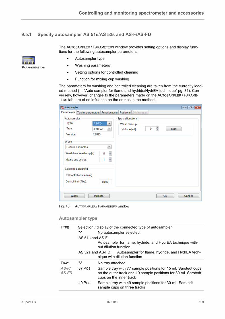
Controlling and monitoring spectrometer and accessories
ASpect LS 07/2015 129
9.5.1 Specify autosampler AS 51s/AS 52s and AS-F/AS-FD
The AUTOSAMPLER / PARAMETERS window provides setting options and display func-tions for the following autosampler parameters:
• Autosampler type
• Washing parameters
• Setting options for controlled cleaning
• Function for mixing cup washing
The parameters for washing and controlled cleaning are taken from the currently load-ed method (→ "Auto sampler for flame and hydride/HydrEA technique" pg. 31). Con-versely, however, changes to the parameters made on the AUTOSAMPLER / PARAME-TERS tab, are of no influence on the entries in the method.
Fig. 45 AUTOSAMPLER / PARAMETERS window
Autosampler type
TYPE Selection / display of the connected type of autosampler "-" No autosampler selected. AS 51S and AS-F
Autosampler for flame, hydride, and HydrEA technique with-out dilution function
AS 52S and AS-FD Autosampler for flame, hydride, and HydrEA tech-nique with dilution function
TRAY AS-F/ AS-FD
"-" No tray attached 87 POS Sample tray with 77 sample positions for 15 mL Sarstedt cups
on the outer track and 10 sample positions for 30 mL Sarstedt cups on the inner track
49 POS Sample tray with 49 sample positions for 30-mL-Sarstedt sample cups on three tracks
PARAMETERS TAB
Controlling and monitoring spectrometer and accessories
130 07/2015 ASpect LS
30 POS Sample tray with 30 positions for 50 mL Sarstedt sample cups on 3 tracks
TRAY AS 51s/ AS 52s
"-" No tray attached 139 POS Sample tray with 129 sample positions for 15 mL Sarstedt
cups on the outer track and 10 sample positions for 30 mL Sarstedt cups on the inner track
54 POS Sample tray with 54 sample positions for 50-mL-Sarstedt sample cups on three tracks
VERSION Version number of autosampler software. Wash
WASH MODE OFF Wash mode switched off. No rinsing performed au-tomatically.
BETWEEN SAMPLE Washes after each sample, but not within a statistical series.
WASH TIME WASH CUP
Time in which the rinsing agent is aspirated in the wash cup.
MIXING CUP CYC-LES
Number of rinse cycles for the mixing cup. In a rinse cycle the mixing cup is filled with wash liquid / diluent and then emptied again.
Controlled cleaning
CONTROLLED CLEANING
Carry out a cleaning wash. The cleaning progress is checked by repeated measurement.
CONTROL LIMIT (ABS.)
The value, to which the signal level must have returned during rinsing, before the diluted samples / samples of lower concentra-tion are analyzed.
Special functions
WASH MIX CUP Wash mix cup separately outside a sequence measurement. VOLUME Enter volume for cleaning. START Wash mixing cup.
9.5.2 Technical parameters of the autosampler AS 51s/AS 52s and AS-F/AS-FD
The AUTOSAMPLER / TECHN.PARAMETERS window allows you to specify:
• depth of submergence of cannula / dosing tube into the various cups
• working speed of dosing unit
• alignment of autosampler arm in relation to sample cups
TECHN. PARAME-
TERS TAB

Controlling and monitoring spectrometer and accessories
ASpect LS 07/2015 131
Fig. 46 AUTOSAMPLER / TECHN. PARAMETERS window
For the individual cup types the following actions are taken into account:
Cup Action SAMPLE CUP
Take up of sample by dosing unit or aspiration by nebulizer (flame technique) or peristaltic pump (hydride technique).
SPECIAL CUP
Take up or aspiration of special samples.
MIX CUP Dosing volume of analyte and diluent, as well as take up of samples after dilution.
WASH CUP Rinsing of cannula and aspiration path (only with flame and hydride technique).
ADD REA-GENT
Elements of the table
ACTION Available action options: TAKE UP – Takes up sample from cup for dispensing into mixing cup or
flame. DISPENSE - Dispenses sample into mixing cup WASH - Takes up wash solution
TYPE Connected autosampler model LOCATION Cup to which a given action refers. DEPTH The depth to which the cannula submerges in units of 1 mm SPEED LEVEL
Designates the working speed of the dosing unit. Greater values cause the dosing unit to work faster, with smaller values it will work more slow-ly. Recommended values: TAKE UP OF SAMPLES Medium speed levels DISPENSE INTO MIXING CUP One of the two highest levels, so that the
Controlling and monitoring spectrometer and accessories
132 07/2015 ASpect LS
fast injection leads to a complete mixing. Besides, the com-plete mix up is supported by a fixed wait time before the take up from the mixing cup (or sample cup).
The take up of diluent and the separating air segment are carried out at fixed speed.
Table subarea Using the controls in the TABLE field, you can change the parameters of the selected table row.
SPEED Speed of dosing unit DEPTH [MM]
Set immersion depth of cannula / dosing tube. The immersion depth is measured from the highest position of the sampler arm.
DEPTH AT POS.
Position of special or sample cup at which the immersion depth is measured.
SET If activated, the sampler arm moves over the cup for which the posi-tioning has to be adjusted. With sample and special cups, this is the position selected under DEPTH AT POS. If not activated, the immersion depth and speed are changed without the sampler arm moving above the cup.
EMPTY MI-XING CUPS
Reset positions of sample cups used for dilution.
9.5.3 Setting insertion depth and dosing speed for AS 51s/AS 52s and AS-F/AS-FD
1. On the AUTOSAMPLER / TECHN. PARAMETERS tab, mark the table row, the parame-ters of which you want to change.
2. For the specification of sample and mixing cups, in the DEPTH AT POS. field, set the position on the tray, at which you want to test the immersion depth.
3. Activate the SET check box to move the sampler arm to the specified cup posi-tion.
4. Watch the movement of the sampler arm and vary the SPEED and DEPTH until you achieve the desired result.
9.5.4 Functional test of the autosampler AS 51s/AS 52s and AS-F/AS-FD
On the AUTOSAMPLER / FUNCTION TESTS tab, you may test the functions of the au-tosampler.
TECHN. PARAME-
TERS TAB
FUNCTION TEST TAB

Controlling and monitoring spectrometer and accessories
ASpect LS 07/2015 133
Fig .47 AUTOSAMPLER / FUNCTION TESTS window
Tracker/Rotator Driving the sampler arm to the various positions:
Option Description CUP NO. Drives to the cup position selected from the corresponding list box. WASH POSITION Drives to the wash cup. MIXING POSITION Only for AS 52s and AS-FD
Drives to the mixing cup Pipetter Only AS 52s and AS-FD
Option Description SPEED Adjust the pipetter speed. VOLUME [µL] Adjust the pipetting volume to be taken up. VALVE TO BOTTLE
Switches the valve to the bottle. The valve switches the flow between the diluent bottle and the sam-ple. In switching, you must hear the valve click.
[TAKE UP] Take up the selected volume with the currently selected pipetter speed.
[DISPENSE] Dispense the selected volume with the currently selected pipetter speed.
[RESET] The volume taken up is dispensed again. Dipping arm Lowering the sampler arm at the position selected under Tracker/Rotator.
Controlling and monitoring spectrometer and accessories
134 07/2015 ASpect LS
DEPTH Adjust the depth by which the sampler arm can be lowered. Pumps
WASH PUMP Start the pump for supply from wash cup. MIXING CUP PUMP Starts the pump for pumping out the mixing cup.
Test programs Tests are provided to test the autosampler with pre-configured, dry running test pro-grams. The cups the sampler arm is driven to during the test must be empty! When the test programs are finished, you are informed of the test success. Start the selected test program with the button [START].
Test program 1 Driving to Position 1 and immersing in cup Rinsing of cannula Driving to Position 33 and immersing in cup Rinsing of cannula Driving to Position 42 and immersing in cup Rinsing of cannula
Test program 2 Execution of Test Program 1 Dispensing 5 mL diluent in mixing cup Rinsing of cannula Drains mixing cup Dispensing 5 mL diluent in mixing cup Rinsing of cannula Drains mixing cup
Error test These tests serve to test the autosampler for sensor errors. If one of the error states listed here appears, every measurement will be aborted (on the screen a correspond-ing error message will be displayed).
The error test is started with the [Test] button. If the test was successful, the indicator will light green; if the test fails, it will light red.
If a test fails, this may have the following causes:
WASH BOTTLE LEVEL Reports excessively low fill level of storage bottle (bottle empty).
DILUENT BOTTLE LE-VEL
Reports excessively low fill level of storage bottle (bottle empty).
TRACKER/ROTATOR Swivel drive of sampler arm and rotary drive of tray are de-fective.
TRAY IDENTIFICATION Sample tray not detected. PIPETTOR (DRIVE) Dosing pump error. PIPETTOR (VOLUME) The volume taken up by the pipettor was too large.
Adjusting the autosampler
[ADJUST SAMP-LER]
Opens the Adjust sampler dialog for readjustment of the au-tosampler.

Controlling and monitoring spectrometer and accessories
ASpect LS 07/2015 135
(→ section "Adjust autosampler AS 51s/AS 52s and AS-F/AS-FD" pg. 135)
9.5.5 Adjust autosampler AS 51s/AS 52s and AS-F/AS-FD
The autosamplers are supplied factory-adjusted.
An adjustment must be carried out in exceptional cases (e.g. following inappropriate transport), if the sampler arm no longer immerses centrally in the cups. Readjustment is carried out computer-controlled in the ADJUST SAMPLER dialog (accessible via THE [ADJUST SAMPLER] button on the AUTOSAMPLER / FUNCTIONAL TEST tab).
Fig.48 Adjust sampler dialog for AS-FD
Options in window ADJUST SAMPLER Selecting the position to be adjusted
MIXING POSITI-ON
Alignment of sampler arm to mixing cup
TRAY POSITION 1
Alignment of sampler arm to sample cup on position 1 of the au-tosampler tray
WASH POSITI-ON
Alignment of sampler arm to wash position (if necessary)
Alignment of mixing position/tray position 1
DEPTH Dipping depth in mm. With this field, the dipping arm can be driven into or out of the particular cup. The immersion depth for MIXING POSITION and TRAY POSITION 1 is no optimizable parameter. The possibility of changing the depth only serves to facilitate assessing the cup center.
DIPPING ARM []/[]
Buttons for changing the sampler arm position. Alternatively, you may press arrow keys "Arrow right" and "Arrow left" on the PC keyboard.
SAMPLER TRAY []/[]
Buttons for rotating the sampler tray. Alternatively, you may use the arrow keys "Arrow up" and "Arrow down" on the PC keyboard.
[SAVE] Saves the new parameters for the selected position. The settings re-main valid until you save new adjustment states.
FUNCTION TEST TAB
Controlling and monitoring spectrometer and accessories
136 07/2015 ASpect LS
Wash pump
LEVEL Adjust wash pump speed level (levels 1-24). [SAVE] Save wash pump speed.
Adjusting the autosampler 1. Place a sample cup on position 1 of the sampler tray.
2. In the ADJUST SAMPLER window, choose the position to be adjusted first.
3. Adjust the immersion depth in a way that the position of the sampler arm relative to the cup can be well assessed.
4. Adjust the position of the sampler arm with the buttons. Additionally for tray position 1: Adjust the position of the sample tray with the but-tons.
5. Save the new parameters in the firmware of the autosampler by clicking on [SAVE].
6. Then, repeat the above steps for the other position.
9.5.6 Position overview in the autosampler AS 51s/AS 52s and AS-F/AS-FD
The sample tray positions used in the current sequence are displayed in AU-TOSAMPLER / POSITION window.
The display modes ALL POSITIONS or ONLY SPECIAL POSITIONS can be selected.
9.5.7 Supply of reagents for sample
In the window AUTOSAMPLER / REAGENT-ADDITION a reagent can be pipetted automati-cally to the samples by using the autosampler AS 52. The reagent must be kept ready in a sample cup on the sample tray. The tab REAGENT ADDITION is only active when a method and a sequence have been loaded.
POSITIONS TAB
TAB REAGENT SUPP-
LY

Controlling and monitoring spectrometer and accessories
ASpect LS 07/2015 137
Fig. 49 AUTOSAMPLER / ADD REAGENT window
1. Enter the following parameters for the reagent:
Option Description NAME Designation of the reagent POSITION Position of reagent on the sample tray. VOLUME [µL] Volume of the reagent which is to be supplied to the samples. CONSIDER FAC-TOR
If activated the dilution factor is taken into consideration by the addition of the reagent.
2. Initialize the sample list with [POS. FROM SEQUENCE].
3. In the sample list enter the analyte volume of the samples.
4. Mark all samples which are to have reagent added with "*".
5. Start the addition of the reagent with [START ADD.].
Controlling and monitoring spectrometer and accessories
138 07/2015 ASpect LS
9.6 Micro pipetter unit MPE 60/AS-GF The autosampler MPE 60 and AS-FG are used as autosampler in the graphite tube and HydrEA technique. There are three versions of the micropipetter unit:
• MPE 60 – autosampler for the graphite tube technique with mixing cup
• MPE 60/1– autosampler without mixing cup
• MPE 60/1 – autosampler without mixing cup
The type of involved autosampler is identified by ASpect LS as part of an initialization routine.
In the AUTOSAMPLER window,
• the connected autosampler model is displayed,
• the autosampler can be adjusted,
• the autosampler can be additionally rinsed / initialized again,
• various functions can be tested.
The parameters directly relevant to the analysis (charging of sample tray, dilution, mixing and wash steps) are to be specified in the method, the sequence and the sam-ple identification data.
Open the AUTOSAMPLER window using menu command METHOD DEVELOPMENT AUTOSAMPLER or the icon button
.
Control buttons in autosampler window
[INITIALIZE] Reinitializes the autosampler. As a general rule, the autosampler is initialized at the beginning of each AAS working session via the MAIN SETTINGS window (→ "Select Analysis Task" pg. 11). It may be necessary to re-initialize the autosampler, if it lost its orientation (e.g. because you pushed against it). Communication between the autosampler, the AAS and the PC will be established.
[WASH] Rinse MPE. Rinsing liquid is pumped through the sample tube via the dosing device and dispensed in the wash cup.
Caution! Connect autosampler only to AAS in deenergized state!
Do not connect the autosampler when the AAS is in power-on condition. Failure to comply may result in faulty communication of even destruction of the interface.
9.6.1 Specify autosampler MPE 60/AS-GF
The AUTOSAMPLER / PARAMETERS window provides setting options and display func-tions for the following autosampler parameters:
• Autosampler type
• Washing parameters
• Setting options for controlled cleaning
METHOD DEVELOP-
MENT AU-
TOSAMPLER...
PARAMETERS TAB
Controlling and monitoring spectrometer and accessories
ASpect LS 07/2015 139
• Function for mixing cup washing
The parameters for WASHING and CONTROLLED CLEANING are taken from the currently loaded method (→ "Autosampler for graphite tube technique (solution analytics)" pg. 34). Conversely, however, changes to the parameters made on the AUTOSAMPLER / PARAMETERS tab, are of no influence on the entries in the method.
Fig. 50 AUTOSAMPLER / PARAMETERS window for AS-GF
Autosampler type
TYPE Selection / display of the connected type of autosampler "-" No autosampler selected. MPE 60 and AS-GF Autosampler for graphite furnace technique
TRAY "-" No tray attached 89 POS for MPE 60
Sample tray with 77 place capacity for 2 mL sample cups, 4 special sample places of 5 mL sample cup volume each and 8 special sample places of 2 mL sample cup volume each
108 POS for AS-GF Probenteller mit 100 Probenplätzen für 1,5-mL-Probengefäße, 4 Sonderprobenplätze und 8 Sonderprobenplätzen mit 5-mL-Probengefäßen
VERSION Version number of autosampler software.
Controlling and monitoring spectrometer and accessories
140 07/2015 ASpect LS
Wash modes
WASH MODE OFF Wash mode switched off. No rinsing performed automati-cally. BETWEEN SAMPLE
Washes after each sample, but not within a statistical series.
BETWEEN RUNS Washes after each measurement, including within a statistical series.
BETWEEN COMPONENTS The autosampler is washed after transfer of each component into the graphite tube (modifier, standard, sample, etc.).
WASH CYCLES WASH CUP
Number of wash cycles per wash, 1 to 5
Controlled cleaning
CONTROLLED CLEANING
Carry out a cleaning wash. The cleaning progress is checked by repeated measurement.
CONTROL LIMIT (ABS.)
The value, to which the signal level must have returned during rinsing, before the diluted samples / samples of lower concentra-tion are analyzed.
Special functions for MPE 60 with mixing cup
WASH MIX CUP Rinse mixing cup separately outside the measurement. VOLUME Enter volume for cleaning. START Wash mixing cup.
MIXING CUP CYCLES
Number of wash cycles for mixing cup. Fills mixing cup with wash liquid/diluent solution and drains it again in one cycle.
9.6.2 Technical parameters of the autosampler MPE 60
The AUTOSAMPLER / TECHN.PARAMETERS window allows you to specify:
• depth of submergence of cannula / dosing tube into the various cups
• working speed of dosing unit
• alignment of autosampler arm in relation to sample cups
• the automatic depth adjustment for volume decrease during the analysis
• the alignment of the MPE 60 to the graphite tube furnace.
TECHN. PARAME-
TERS TAB

Controlling and monitoring spectrometer and accessories
ASpect LS 07/2015 141
Fig. 51 AUTOSAMPLER / TECHN. PARAMETERS window tab for MPE 60
Actions for cup types For the individual cup types the following actions are taken into account:
SAMPLE CUP Take up samples through doser. SPECIAL CUP Take up special samples. MIX CUP Dosing volume of analyte and diluent, as well as take up of samples
after dilution. WASH CUP Rinsing of cannula. GRAPHITE TU-BE
Inject sample or special sample into the graphite tube.
Elements of the table
ACTION Available action options: TAKE UP – Draws in sample from sample cup, special cup or mixing cup. DISPENSE - Dispenses sample into mixing cup INJECT - Inject sample or special sample into the graphite tube. DISPENSE SPECIAL
TYPE Type of connected autosampler LOCATION Cup to which a given action refers. DEPTH The depth to which the cannula submerges in units of 1 mm SPEED LEVEL
Designates the working speed of the dosing unit. Greater values cause the dosing unit to work faster, with smaller values it will work more slow-ly. Recommended settings: SAMPLE TAKE-UP 3 DISPENSING TO MIXING CUP 9 INJECTION INTO GRAPHITE TUBE 1

Controlling and monitoring spectrometer and accessories
142 07/2015 ASpect LS
Table subarea Using the controls in the TABLE field, you can change the parameters of the selected table row.
SPEED Speed of dosing unit DEPTH [MM]
Set immersion depth of cannula / dosing tube. The immersion depth is measured from the highest position of the sam-pler arm.
DEPTH AT POS.
Position of special or sample cup at which the immersion depth is meas-ured.
SET If activated, the sampler arm moves over the cup for which the position-ing has to be adjusted. With sample and special cups, this is the position selected under DEPTH AT POS. If not activated, the immersion depth and speed are changed without the sampler arm moving above the cup.
Automatic depth correction
AUTOMAT. DEPTH COR-RECTION
Automatically adapts the depth, to which the dosing tube will sub-merge into sample or special cups, to a new volume.
[SAMPLE CUPS] Only active if AUTOMAT. DEPTH CORRECTION is active. Opens the SAMPLER POSITION, VOLUMES and DEPTHS window to al-low settings for non-standard container geometries and volumes of individual cups. These settings will be taken into account for auto-matic depth correction (→ "Automatic depth correction for MPE 60 and AS-GF" pg. 143).
Over functions
FURNACE LED/FURNACE
CAMERA
[OPEN FUR-NACE]/[CLOSE FUR-NACE]
Open and close furnace.
[ALIGN MPE TO FUR-NACE]
On selection of this control button, the screen-driven proce-dure for alignment of the MPE in relation to the graphite tube furnace will be triggered (→ "Aligning MPE 60 to graphite tube furnace" pg. 145").
[EMPTY MIXING CUPS] Nur MPE 60/2 und AS-GF Nur aktiv, wenn Probengefäße als Mischgefäße verwendet wurden. Die im Fenster METHODE / PROBENZUFUHR definier-ten Positionen werden für eine erneute Verwendung freige-geben.
Controlling and monitoring spectrometer and accessories
ASpect LS 07/2015 143
9.6.3 Set insertion depth and dosing speed of the MPE 60 and AS-FG
1. On the AUTOSAMPLER / TECHN. PARAMETERS tab, mark the table row, the parame-ters of which you want to change.
2. For the specification of sample and mixing cups, in the DEPTH AT POS. field, set the position on the tray, at which you want to test the immersion depth.
3. Activate the SET check box to move the sampler arm to the specified cup posi-tion.
4. Watch the movement of the sampler arm and vary the SPEED and DEPTH until you achieve the desired result.
9.6.4 Automatic depth correction for MPE 60 and AS-GF
The purpose of automatic correction of the depth level to which the dosing tube will submerge into a sample cup or a special cup is to prevent unwanted contamination of the dosing tube. To draw in a sample volume, the dosing tube will dip into a sample cup just as much as necessary to accomplish this. As total volume removal increases, the immersion depth will automatically be corrected.
The AUTOSAMPLER / TECHN. PARAMETERS window contains immersion depth settings for sample cups and special cups that will initially apply to any cup on the sample tray.
Fill volumes or cup sizes at variance with standard cups can be separately specified and duly considered for automatic depth correction.
1. Activate the AUTOMAT. DEPTH CONTROL checkbox in the AUTOSAMPLER / TECHN. PARAMETERS window.
2. Click on [SAMPLE CUPS].
The SAMPLER POSITIONS, VOLUMES AND DEPTHS window will show.
Fig. 52 POSITIONS, VOLUMES AND DEPTHS window for MPE 60
TECHN. PARAME-
TERS TAB
TECHN. PARAME-
TERS TAB

Controlling and monitoring spectrometer and accessories
144 07/2015 ASpect LS
3. With regard to individual special cups or sample cups, the following parameters can be specified:
POSITION Set cup position on the tray, for which the three displayed values: volume, depth and diameter apply. Settings must be made indi-vidually for each cup that is intended to be modified.
VOLUME Displays the amount of sample volume already retrieved from a cup or allows input of lacking sample volume balance into a cup not completely filled. This reading is software-updated after each sample take-in se-quence.
DEPTH Displays the amount of additional depth due to overall sample withdrawal up to this moment. This value is recalculated after each sample take-in sequence. Total immersion depth is the sum of a specified immersion depth (DEPTH column on TECHN. PARAMETERS tab) and the additional depth shown here.
DIAMETER Indicates the cup diameter. This value is used as input for calculation of the depth, based on the amount of withdrawn volume.
DIAMETER checkbox
For cups with dimensions at variance against those of standard cups. Allows you to specify a diameter for each cup individually if marked.
[DELETE VO-LUMES]
Resets volume values for all special cups or sample cups to 0.
[RESET] Resets all volumes and the depth values of all cups to 0, resets diameters to their latest via [OK] saved values.
Maximum dipping depth (auto correction) A maximum allowed immersion depth can be specified in order to prevent the dosing tube from hitting the cup bottom and getting twisted.
SAMPLE CUPS
Applies settings for maximal immersion depth to sample cups if marked.
SPECIAL CUPS
Applies settings for maximal immersion depth to special cups if marked.
DEPTH [MM]
Defines the maximal allowed immersion depth of the autosampler into a sample cup or special cup. Caution: Please note that the autosampler will at once dip down to the new depth level if the SET checkbox is marked! Make sure that the au-tosampler motion path is not blocked. A modified setting for immersion (dipping) depth should be saved with [SAVE].
POSITION The sample tray position in which immersion depth settings are checked.

Controlling and monitoring spectrometer and accessories
ASpect LS 07/2015 145
SET The dosing tube will dip into a cup that was specified via POSITION and to a depth that was set via DEPTH [MM]. The immersion depth can be visually checked. Caution: When the check box SET is marked, the autosampler will be dipped immediately to the given depth! Make sure that the autosampler motion path is not blocked.
9.6.5 Aligning MPE 60 to graphite tube furnace The process for MPE alignment in relation to the graphite tube furnace with subse-quent setting of dosing tube immersion depth into the graphite tube is program-guided.
1. Actuate [ALIGN MPE TO FURNACE] in AUTOSAMPLER / TECHN. PARAMETERS window.
2. Follow further instructions on the monitor screen.
The autosampler is correctly aligned to the graphite tube furnace.
1 Alignment screw 1
2 Counterlocking nut of alignment screw 1
3 Alignment screw 2
4 Adjustment aid with crosshair
5 Autosampler arm 6 Alignment screw
3 7 Counterlocking
nut of alignment screw 3
Fig. 53 Alignment of autosampler MPE 60
TECHN. PARAME-
TERS TAB

Controlling and monitoring spectrometer and accessories
146 07/2015 ASpect LS
9.6.6 Function test of autosampler On the AUTOSAMPLER / FUNCTION TESTS tab, you may test the functions of the au-tosampler.
Fig. 54 AUTOSAMPLER / FUNCTION TESTS window
Tracker/Rotator
Driving the sampler arm to the various positions:
CUP NO. Drives to the cup position selected from the corresponding list box. WASH POSITION Drives to the wash cup. MIXING POSITION Move the mixing cup (for MPE 60). TUBE POSITION Move graphite tube.
Pipetter
SPEED Adjust the pipetter speed (→ "Setting insertion depth and dosing speed for AS 51s/AS 52s and AS-F/AS-FD" pg. 132).
VOLUME [µL] Adjust the pipetting volume to be taken up. VALVE TO BOTTLE
Switches the valve to the bottle. The valve switches the flow between the diluent bottle and the sam-ple. In switching, you must hear the valve click.
[TAKE UP] Take-up the selected volume with the currently selected pipetter speed.
[SISPENSE] Dispense the selected volume with the currently selected pipetter speed.
[RESET] The volume taken up is dispensed again.
FUNCTION TEST TAB
Controlling and monitoring spectrometer and accessories
ASpect LS 07/2015 147
Dipping arm Lowering the sampler arm at the position selected under Tracker/Rotator.
DEPTH Adjust the depth by which the sampler arm can be lowered. Pumps
WASH PUMP Start the pump for supply from wash cup. MIXING CUP PUMP Starts the pump for pumping out the mixing cup.
Test programs Tests are provided to test the autosampler with pre-configured, dry running test pro-grams. The cups the sampler arm is driven to during the test must be empty!
When the test programs are finished, you are informed of the test success.
Start the selected test program with the button [START].
TEST PROGRAM 1 Aspirates volume from position 1 Aspirates volume from position 41 Discharges volume into graphite tube Washes dosing tube two times
TEST PROGRAM 2 Aspirates diluent solution from waste bottle Aspirates volume from position 10 Discharges volume into mixing cup Aspirates volume from mixing cup Discharges volume into graphite tube Washes dosing tube Drains mixing cup Washes and drains mixing cup
Error test These tests serve to test the autosampler for sensor errors. If one of the error states listed here appears, every measurement will be aborted (on the screen a correspond-ing error message will be displayed).
The error test is started with the [TEST] button. If the test was successful, the indicator will light green; if the test fails, it will light red.
If a test fails, this may have the following causes:
WASH BOTTLE LEVEL Reports excessively low fill level of storage bottle (bottle emp-ty).
WASTE BOTTLE LE-VEL
Fill level of waste bottle is too high (bottle is full).
TRACKER/ROTATOR Swivel drive of sampler arm and rotary drive of tray are defec-tive.
TRAY IDENT. Sample tray not detected. PIPETTER (DRIVE) Dosing pump error. PIPETTER (VOLUME) The volume taken up by the pipettor was too large.
Controlling and monitoring spectrometer and accessories
148 07/2015 ASpect LS
Button [ADJUST SAMPLER] With [ADJUST AUTOSAMPLER] the positioning of the autosampler arm to the various cups of the autosampler is adjusted (→ "Adjusting the MPE 60/AS-FD" pg. 148).
9.6.7 Adjusting the MPE 60/AS-FD
The autosamplers are supplied factory-adjusted.
An adjustment must be carried out in exceptional cases (e.g. following inappropriate transport), if the sampler arm no longer immerses centrally in the cups. Readjustment is carried out computer-controlled in the ADJUST SAMPLER dialog (accessible via the [ADJUST SAMPLER] button on the AUTOSAMPLER / FUNCTIONAL TEST tab).
Fig. 55 Adjust autosampler window for MPE 60
Selecting the position to be adjusted for MPE 60
MIXING POSITI-ON
Alignment of sampler arm to mixing cup
TRAY POSITION 1
Alignment of sampler arm to sample cup on position 1 of the au-tosampler tray
WASHING DEPTH
Insertion depth of cleaning cup
Selecting the position to be adjusted for AS-GF
MIXING POSITI-ON
Alignment of sampler arm to mixing cup
TRAY POSITION 1
Alignment of sampler arm to sample cup on position 1 of the au-tosampler tray
WASHING DEPTH
Insertion depth of cleaning cup
TECHN. PARAME-
TERS TAB
Controlling and monitoring spectrometer and accessories
ASpect LS 07/2015 149
Alignment of position
DEPTH [MM] Dipping depth in mm. With this field, the dipping arm can be driven into or out of the particular cup. The immersion depth is no optimizable pa-rameter. The possibility of changing the depth only serves to facilitate assessing the cup center.
DIPPING ARM []/[]
Buttons for changing the sampler arm position. Alternatively, you may press arrow keys "Arrow right" and "Arrow left" on the PC keyboard.
SAMPLER TRAY []/[]
Buttons for rotating the sampler tray. Alternatively, you may use the arrow keys "Arrow up" and "Arrow down" on the PC keyboard.
[SAVE] Saves the new parameters for the selected position. The settings re-main valid until you save new adjustment states.
Adjustment of depth in the washing cup for MPE 60
DEPTH [MM] Depth of submergence into wash cup in units of 1 mm. [SAVE] Saves immersion depth in wash cup.
Adjusting the autosampler for MPE 60 1. Place a sample cup on position 1 of the sampler tray.
2. In the ADJUST SAMPLER dialog, choose the position to be adjusted first.
3. Adjust the immersion depth in a way that the position of the sampler arm relative to the cup can be well assessed.
4. Adjust the position of the sampler arm with the buttons. Additionally for tray position 1: Adjust the position of the sample tray with the but-tons.
5. Save the new parameters in the firmware of the autosampler by clicking on [Save].
6. Then, repeat the above steps for the other position.
9.6.8 Position overview of the MPE 60 and AS-GF
The sample tray positions used in the current sequence are displayed in window SAM-PLER / POSITION.
The display modes ALL POSITIONS or ONLY SPECIAL POSITIONS can be selected.
9.7 Solid autosampler SSA 600 To run automated solid analytical procedures, the SSA 600 is applied. The type of involved autosampler is identified by ASpect LS as part of an initialization routine. The SOLID SAMPLER window provides functions as follows:
• SSA 600 function test
• Alignment of SSA 600 to graphite tube furnace
POSITIONS TAB
METHOD DEVELOP-
MENT / AU-
TOSAMPLER...
Controlling and monitoring spectrometer and accessories
150 07/2015 ASpect LS
As the solid autosampler SSA 600 can be operated with and without liquid dosing, the functional test and the adjustment are aligned to the autosampler specified in the method.
Open the METHODS window with the symbol .
Select any analysis line on the LINES tab and activate the option SSA 600 WITH AUTOMATIC LIQUID PIPETTER on the tab SAMPLE SUPPLY
Activate settings with [ACCEPT].
Use a METHOD DEVELOPMENT / AUTOSAMPLER... menu command or click the
icon to open the SOLID SAMPLERwindow.
Control buttons in autosampler window
[RESET] Take up sample platforms which are on various positions of the au-tosampler and transport back to the sample tray.
[INITIALIZE] Reinitializes the autosampler. As a general rule, the autosampler is initialized at the beginning of each AAS working session via the PRELIMINARY SETTINGS window (→"Preparative Settings" pg. 11). It may be necessary to re-initialize the autosampler, if it lost its orientation (e.g. because you pushed against it). Communication between the autosampler, the AAS and the PC will be established.
[ALIGN] Triggers a routine to align the SSA 600 to the graphite tube furnace.
Caution! Connect autosampler only to AAS in deenergized state!
Do not connect the autosampler when the AAS is in power-on condition. Failure to comply may result in faulty communication of even destruction of the interface.
Sample preparation items which are different from those in solution analytics (deter-mination of sample platform deadweight, dosing and weighing of sample) can be specified on the SOLID tab (→ "Displaying details of single values of samples" pg. 78).

Controlling and monitoring spectrometer and accessories
ASpect LS 07/2015 151
9.7.1 Function test of solid sampler Working in the SOLID SAMPLER – FUNCTION TEST window, you may check individual functions.
Fig.56 SOLID SAMPLER – FUNCTION TEST window
STATUS / BUTTONS
Displays SSA 600 status and button that was actuated since the lat-est query in appropriate color (green, orange, red). Using [UPDATE], the status can be queried again and the button dis-play be updated.
MOVE TO PO-SITION
Performs motion to the position selected via the POS. list field. Thus no platform is taken up or put down.
ROTATE TRAY Rotates the sample tray into a selected position. TRANSPORT Means that SSA 600 transports a platform from a given position to
the next starting and target position. If TAKE-UP PLATFORM is activated, the gripper will pick up a platform. If PUT-DOWN PLATFORM is activated, the gripper will place a platform down in its target location.
GRIPPER Opens or closes the gripper. LOWER CAN-NULA
Moves the cannula downwards.
BALANCE Determines the weight of a platform in a specified position on the tray (POS.) WEIGHING WITH TARE
Before a platform can actually be weighed, the scale must be tared. #1 indicates the tared weight. #2 contains the weight of the platform (also with dosed sample as may be the case).
[INTERNAL CALIBRATION] During a calibration cycle of this type, the internal calibra-tion graph of the scales is redetermined. To achieve this, the scales are initially reset, their zero-
FUNCTION TEST TAB

Controlling and monitoring spectrometer and accessories
152 07/2015 ASpect LS
point is determined and an internal weight is weighed. The values obtained for zero-point and internal weight will provide the input for determination of the scales calibra-tion graph.
LOOP The autosampler transports two platforms (positions 1 and 2) in both directions between the sample tray, the scales and the furnace. The number of transporting cycles can be specified via the CYCLES input field.
9.7.2 Alignment of solid sampler The SOLID SAMPLER / ALIGNMENT window provides functions as follows:
• Control and adjustment of motion to individual autosampler positions
• Adjustment of the SSA 600 to the position of the graphite tube furnace
• SSA 600 with dosing unit: Automatic depth correction for taking in matrix mod-ifiers and special liquid samples.
• Test of liquid dosing
Fig.57 SOLID SAMPLER / ALIGNMENT window
POSITIONS TO ADJUSTED Selection of the position on the autosampler BUTTONS IN GROUP ADJUST POSITION
Alignment of the gripper to the set adjustment position
[OPEN GRIPPER]/[CLOSE GRIPPER]
Open and close gripper with software control, e.g. for changing the gripper tips.
[LOWER CANNULA] For liquid dosing Lower cannula.
GROUP AUTOMATIC DEPTH ADJUSTMENT
Settings for the automatic depth adjustment for the liquid dosing
ADJUSTMENT TAB
Controlling and monitoring spectrometer and accessories
ASpect LS 07/2015 153
[WASH] Wash dosing tube with the pre-set and with con-firmed number WASH CYCLES.
[TEST LIQUID DOSING] Check liquid dosing. [CHANGE DOSING SYRINGE ] Moves the piston of the dosing device downwards in
order to enable changing the dosing device.
Monitoring & aligning individual positions 1. Select a desired position from the POSITION TO ADJUST list.
2. Click [MOVE TO] in ALIGN POSITION group, in order to move the autosampler to the selected position. Put a platform up in this position and check the position of the platform.
3. Use control buttons in this group to make positional corrections as necessary.
4. Save all modified setting by clicking the related [SAVE] button.
Align gripper to the graphite tube furnace The adjustment aids matched to the furnace type are used for the adjustment of the gripper to the graphite tube furnace.
The adjustment is controlled by software and it is started with [ALIGN] in the au-tosampler window.
There is a detailed description in the "Solid Autosampler SSA 600" operating instruc-tions.
Rinsing the system Only for SSA 600 with liquid dosing.
When cleaning the system diluent is taken from the supply bottle and pumped through the entire path via the dosing device to the dosing tube and dispensed into the wash cup.
1. Enter the number of repetitions in the entry field WASH CYCLES.
2. Save the entry with the symbol .
3. Use the [WASH] button to start the wash cycle.
Automatic depth correction for dosing unit
Typically, depth correction occurs automatically when working with an SSA 600, i.e. as the volume that is drawn from dosing unit cups increases, the immersion depth will be matched accordingly. Starting volumes other than those which were set via Method can be corrected in this window. These settings are similar to those for MPE 60/AS-GF (→ "Automatic depth correction for MPE 60 and AS-GF" p. 143).
Adapt ASpect LS
154 07/2015 ASpect LS
10 Adapt ASpect LS
10.1 General settings In the OPTIONS window, you can choose the following settings, which apply to the complete operation of ASpect LS:
• View options
• Save paths of files
• Parameters for data export
• General measurement settings
The options selected in this window remain set after exiting and restarting ASpect LS.
Activate the OPTIONS window with menu command EXTRAS OPTIONS or by a click
on the
button.
Alternatively, in the Main settings window, you may activate the Options option button in the Task field and click on [OK] (→ "Select Analysis Task" pg. 11).
10.1.1 View options 1. In the OPTIONS / VIEW window, define the functions and elements that shall be
accessible on the workspace.
Fig.58 OPTIONS /VIEW window
EXTRAS OPTIONS...
VIEW TAB

Adapt ASpect LS
ASpect LS 07/2015 155
Display
SHOW TOOLBAR Shows the toolbar. SHOW ICON BAR Shows the icon bar at the selected position.
(The position of the icon bar may also be changed by dragging it with the mouse. However, this setting will not be saved).
HIDE EVENT WINDOWS If activated, the yellow event windows (e.g. delay time) will not be displayed. Instead of this, the messages appear in the status bar of the main window.
SUBWINDOWS CAN BE MAXIMIZED
In subwindows (MDI window) activate the Maximize sys-tem button (rectangle). In this way the windows can be maximized to the size of the main window.
HIDE RESULT WINDOWS AUTOMATICALLY
Results windows are blanked if subwindows (e.g. method window) are opened. After shutting the subwindows the result windows are displayed again.
DISPLAY TOOL TIPS Displays brief help texts (tool tips) while pointing on an icon button as well as on the table headers in windows METHOD, SEQUENCE and SAMPLE ID.
ALLOW SCREENSAVER Allows the screensaver. LISTS AND SIGNAL CO-LORS
A click on the [...] button opens the color selection dialog. There, you may choose predefined or newly defined col-ors as list background.
USE PRTSCR KEY FOR HARDCOPY (INSTEAD F5)
By default, the printout of the hardcopy of the screen is started with [F5]. In this case, the [PRTSCR] key of the keyboard is used for the Windows clipboard function. If this checkbox is activated, the [PRTSCR] button starts the printout of the screen hardcopy. This function becomes active only after restarting ASpect LS.
With the [DEFAULT SETTINGS] button, all currently set options are reset to default set-tings.
10.1.2 Save paths The save paths selected for the program and the files during installation are displayed in the OPTIONS / FOLDER window.
PROGRAM Installation path of executable files. WORK DIRECTO-RY
Directory for user data. The work folder contains further subfold-ers. The work directory is defined during installation or through set-tings in User Management.
TEMPORARY DATA Folder for files created temporarily by the application. SAMPLE INFOR-MATION
Default path for opening and saving sample information files. This path may be changed. When opening and saving the sam-ple information data a deviating path can be selected.
FOLDER TAB
Adapt ASpect LS
156 07/2015 ASpect LS
EXPORT/IMPORT Default path for the export and import of method and sequence data. This path may be changed. When exporting and importing a de-viating path can be selected.
RESULTS Folder for results files. This default folder may contain additional subfolders for result storage. These folders are available for sav-ing results files at the start of measurements.
APPLICATION DA-TA
List for data in which ASpect LS stores necessary data.
With the [ADD…] button, you can create new subfolders to the RESULTS folder for sav-ing results. Besides, it is possible to delete and rename empty folders here.
10.1.3 Export options In the OPTIONS / ASCII/CSV EXPORT window, you can define the parameters for ex-porting results to ASCII files. The parameters apply for both forms of the data export, for the automatically continuous and also the manually (→ "Saving results in ASCII/CSV format" pg. 172).
Settings
DECIMAL SEPARA-TOR
Defines the separator for decimal numbers.
LIST SEPARATOR Defines the character separating the individual elements of a list.
In the RESULT FIELDS FOR EXPORT field, you may define which columns of the result table shall be exported to the ASCII file. ALLexports all columns of the selected and non-selected tables of the result list, ONLY SELECTED FIELDS opens a list in which you can choose the columns to be exported.
A click on the [DEFAULT SETTINGS] button resets all options and stored window loca-tions to default settings.
10.1.4 Options for continuous ASCII export In the window OPTIONS / CONTINUOUS ASCII-EXPORTthe export of
results data during the analysis sequence is activated. The export file is updated re-spectively after the output of a new line in the process and result window. The result data will be appended to already existing files.
Further export options may be defined in the OPTIONS - ASCII/CSV EXPORT window.
The export function is activated by selecting the CONTINUOUS ASCII EXPORT OF RE-SULTS DATAcheckbox.
File name
"METHOD DESIGNATI-ON".CSV
The file name corresponds to the name of the method. The file name extension is ".csv". The file is saved to the default EXPORT/IMPORT path (OPTIONS - PATHS).
ASCII/CSV-EXPORT
CONTINUOUS ASCII-EXPORT

Adapt ASpect LS
ASpect LS 07/2015 157
"RESULTS FILE NA-ME".CSV
The file name corresponds to the name of the results file. The file name extension is ".csv". The file is saved to the default EXPORT/IMPORT path (OPTIONS - PATHS).
OTHER You may freely define file name and save path. A click on the [...] button opens the file selection dialog for the selection of an existing file.
10.1.5 Options for analysis sequence In the OPTIONS / ANALYSIS SEQUENCE window, you can define general options for the analysis process.
Fig. 59 OPTIONS / ANALYSIS SEQUENCE window
Stop after following errors
INVALID CALIBRATION FUNCTION
If activated, the analysis sequence will be stopped if the cal-ibration function could not be calculated.
Additional error checks
MONOTONY OF CALIB-RATION POINTS
If activated, the calibration points will be tested for monoto-ny. The monotony test serves to determine if higher standard concentrations also lead to higher measured values.
AUTOSAMPLER LEVEL SENSORS
If activated, the signals from the fill level sensor of the au-tosampler and the waste bottle will be queried.
AUTOZERO DRIFT CHECK Check the absorbance drift during the autozero phase. Display windows
TAB ANALYSIS SE-
QUENCE

Adapt ASpect LS
158 07/2015 ASpect LS
SIGNAL PLOT If activated, a window is displayed during the analysis process showing the curve of the measured signal (e.g. absorbance curve) as a function of time.
WITH FURNACE PROGRAM
Im Signalverlauf wird der temperaturverlauf des Ofenprogramms eingezeichnet.
BARGRAPH Show measured absorption or emission as bargraph. SCALING OF MAX. SIGNAL VALUE
Defines the maximum of the measurement value axis for the presentation of the signal curve. AUTO: Automatic scaling of signal axis. (Alternatively, you may set this option also via menu function VIEW / SCALE (ABS).)
REPORT WINDOW
If activated, a window is displayed during the analysis process showing status information on the used atomizer (flame, graphite tube furnace, hydride system).
SAMPLE CONC. IN CALIBRATION CURVE
If activated, the SAMPLE CONC. IN CALIBRATION CURVE window is dis-played with the current calibration, and if measured already, the recalibration curve. After the measurement of the sample, the cal-culation of the uncorrected concentration from absorb-ance/emission data is illustrated by red auxiliary lines. If addition calibration is used, the converted calibration curve will be dis-played.
FURNACE CAMERA
Keeps the furnace camera’s photograph of the graphite furnace permanently superimposed for viewing at the display screen, until the preset furnace control temperature TEMPERATURE FOR SHUTTER TO OPEN has been reached (→ "Further furnace functions" pg. 121). This allows you to directly watch as a sample droplet is deposited and drying.
Other
ATTACH DATE/TIME TO THE RESULTS FILENAME
Current PC/time at the start of measurement are auto-matically attached to the name of the result file.
MIN. LAMP PRE-HEATING TIME (ROUTINE) [MIN]
Defines the automatically controlled pre-heating time for the lamp. The pre-heating time can be de-activated.
DISPLAY R INSTEAD OF R2(ADJ.) FOR CALIBRATION DATA
Display the R correlation statistics instead of R2(adj.) for the calibration curve.
BEEP AFTER END OF COOL-ING PHASE
Only for graphite tube technique A beep will sound as soon as the graphite tube has completely cooled down.
TAKE-UP COMPONENTS DURING COOLING PHASE
Only for graphite tube technique While the graphite tube cools down, the MPE takes up next samples. This option may be used to accelerate a measuring sequence.
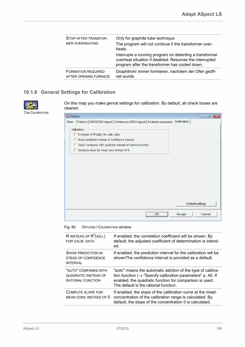
Adapt ASpect LS
ASpect LS 07/2015 159
STOP AFTER TRANSFOR-MER OVERHEATING
Only for graphite tube technique The program will not continue if the transformer over-heats. Interrupts a running program on detecting a transformer overheat situation if disabled. Resumes the interrupted program after the transformer has cooled down.
FORMATION REQUIRED AFTER OPENING FURNACE
Graphitrohr immer formieren, nachdem der Ofen geöff-net wurde.
10.1.6 General Settings for Calibration On this map you make genral settings for calibration. By default, all check boxes are cleared.
Fig. 60 OPTIONS / CALIBRATION window
R INSTEAD OF R2(ADJ.) FOR CALIB. DATA
If enabled, the correlation coefficient will be shown. By default, the adjusted coefficient of determination is intend-ed.
SHOW PREDICTION IN-STEAD OF CONFIDENCE INTERVAL
If enabled, the prediction interval for the calibration will be shownThe confidence interval is provided as a default.
"AUTO" COMPARES WITH QUADRATIC INSTEAD OF RATIONAL FUNCTION
"auto" means the automatic selction of the type of calibra-tion function (→ "Specify calibration parameters" p. 40. If enabled, the quadratic function for comparison is used. The default is the rational function.
COMPUTE SLOPE FOR MEAN CONC INSTAED OF 0
If enabled, the slope of the calibration curve at the mean concentration of the calibration range is calculated. By default, the slope of the concentration 0 is calculated.
TAB CALIBRATION
Adapt ASpect LS
160 07/2015 ASpect LS
10.2 Specifying units, QC and stock standards In the DATA window, the units available for the entire application as well as frequently used stock standards and QC samples are managed.
To activate the DATA window, activate menu command EXTRAS DATA MANAGE-MENT... or click on symbol button
.
10.2.1 Specifying units of measurements You can define the units of measurement available throughout the application in the DATA / UNITS window.
There are 3 preferred variations (for solutions: mg/L, µg/L, ng/L; for solid samples: mg/kg, µg/kg, ng/kg) available. These units cannot be changed by the user. Units deviating from these can be freely defined. For freely defined units it is necessary to enter the conversion factor under FACTOR:
UNIT Name of the unit (max. 10 characters) COMMENT Remarks on the unit (max. 20 characters) FACTOR Factor 1 corresponds to 1 µg/L or µg/kg, factor 1000 corresponds to 1
ng/L or ng/kg TYPE solid = unit used for a solid sample, liquid = unit used for a liquid sample
(solution) The [APPEND] and [INSERT] buttons serve to append user-defined units to the end of the list or insert them above the currently selected row. With the [DELETE BUTTON], you can delete user-defined units, the preferred default units, however, cannot be deleted. To permanently save any changes on this tab, click on [SAVE].
10.2.2 Specifying stock standards and QC samples The composition of frequently used stock standards and QC samples is managed under DATA / STOCK STD/QC SAMPLES.
The compositions of these frequently used single and multielement standards are then available throughout the application.
EXTRAS DATA
MANAGEMENT...
UNITS TAB
TAB STOCK-STD/QC-SAMPLES
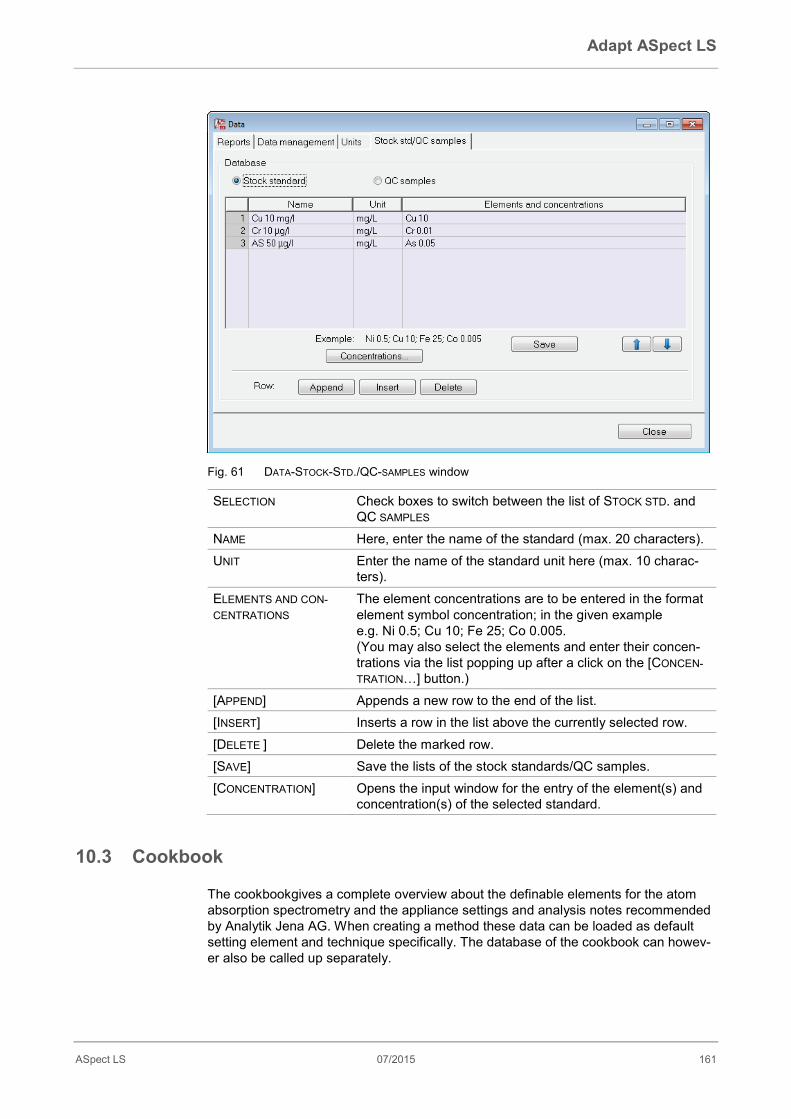
Adapt ASpect LS
ASpect LS 07/2015 161
Fig. 61 DATA-STOCK-STD./QC-SAMPLES window
SELECTION Check boxes to switch between the list of STOCK STD. and QC SAMPLES
NAME Here, enter the name of the standard (max. 20 characters). UNIT Enter the name of the standard unit here (max. 10 charac-
ters). ELEMENTS AND CON-CENTRATIONS
The element concentrations are to be entered in the format element symbol concentration; in the given example e.g. Ni 0.5; Cu 10; Fe 25; Co 0.005. (You may also select the elements and enter their concen-trations via the list popping up after a click on the [CONCEN-TRATION…] button.)
[APPEND] Appends a new row to the end of the list. [INSERT] Inserts a row in the list above the currently selected row. [DELETE ] Delete the marked row. [SAVE] Save the lists of the stock standards/QC samples. [CONCENTRATION] Opens the input window for the entry of the element(s) and
concentration(s) of the selected standard.
10.3 Cookbook The cookbookgives a complete overview about the definable elements for the atom absorption spectrometry and the appliance settings and analysis notes recommended by Analytik Jena AG. When creating a method these data can be loaded as default setting element and technique specifically. The database of the cookbook can howev-er also be called up separately.

Adapt ASpect LS
162 07/2015 ASpect LS
Open the cookbook with the symbol in the tool bar or use the menu com-mand METHOD DEVELOPMENT COOKBOOK.
Fig .62 COOKBOOK window
Display and operating elements in the cookbook window
TECHNIQUE Choice of atomization technique used ELEMENT Selection list of the elements to be analyzed with the selected
technique "Info" – gives general information on analyses with the selected atomization technique.
WINDOW DIS-PLAY
Information on the analysis
[<<]/[[>>] Scroll between the window pages.
METHOD DEVELOP-
MENT COOKBOOK
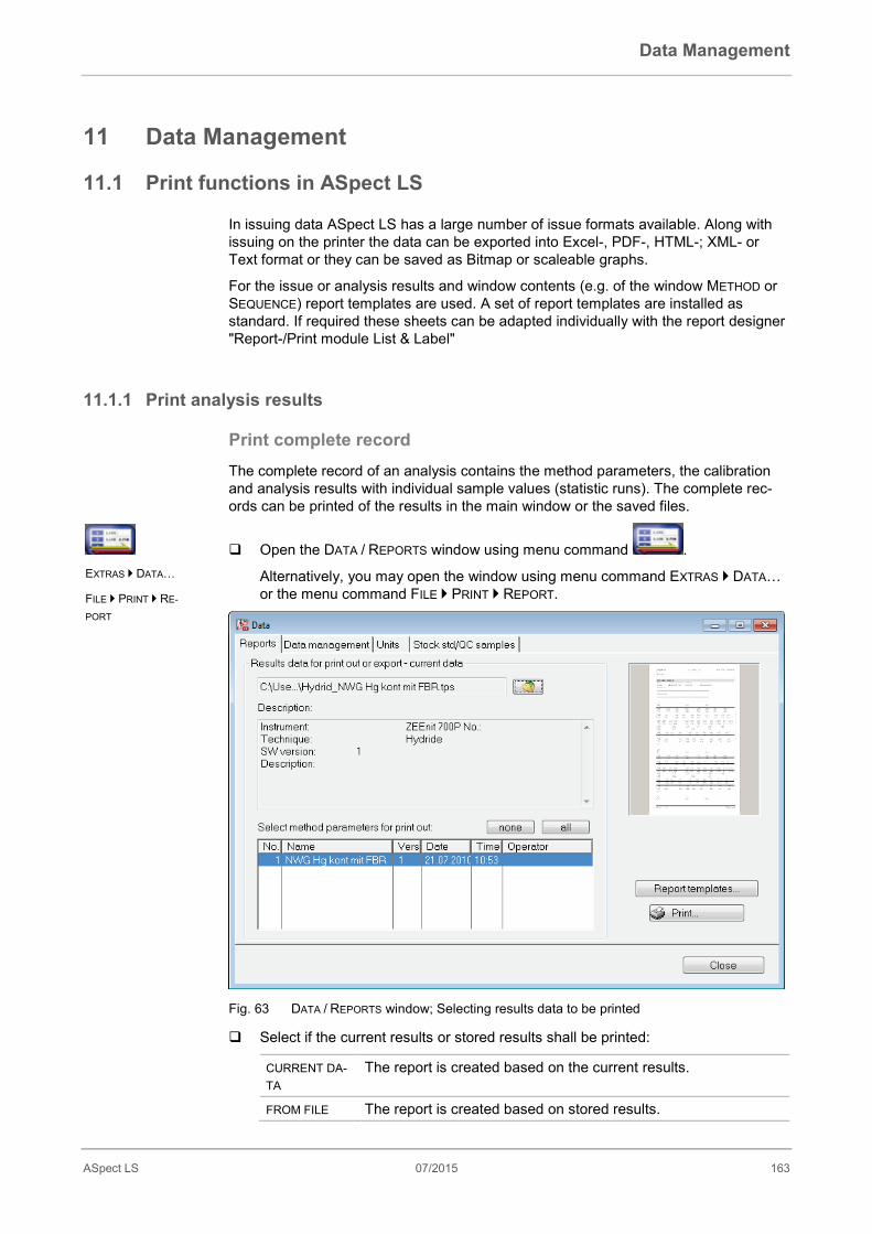
Data Management
ASpect LS 07/2015 163
11 Data Management
11.1 Print functions in ASpect LS In issuing data ASpect LS has a large number of issue formats available. Along with issuing on the printer the data can be exported into Excel-, PDF-, HTML-; XML- or Text format or they can be saved as Bitmap or scaleable graphs.
For the issue or analysis results and window contents (e.g. of the window METHOD or SEQUENCE) report templates are used. A set of report templates are installed as standard. If required these sheets can be adapted individually with the report designer "Report-/Print module List & Label"
11.1.1 Print analysis results Print complete record The complete record of an analysis contains the method parameters, the calibration and analysis results with individual sample values (statistic runs). The complete rec-ords can be printed of the results in the main window or the saved files.
Open the DATA / REPORTS window using menu command .
Alternatively, you may open the window using menu command EXTRAS DATA… or the menu command FILE PRINT REPORT.
Fig. 63 DATA / REPORTS window; Selecting results data to be printed
Select if the current results or stored results shall be printed:
CURRENT DA-TA
The report is created based on the current results.
FROM FILE The report is created based on stored results.
EXTRAS DATA…
FILE PRINT RE-
PORT
Data Management
164 07/2015 ASpect LS
With , open the OPEN standard window and choose the de-sired file.
DESCRIPTION This field shows information on the selected results file. METHODS This table displays the method that belongs to the results file
(only if the method is currently loaded or it was saved along with the results file).
With saved files you can mark all methods which are to be issued in the report in
the methods list.
Open the window ASPECT LS RECORD with [PRINT].
If necessary change the issue format in the list OUTPUT OPEN... and set special parameters of the output format with [OPTIONS]
Start the printout using [START].
Printing the main window result tabs Activate the tab in the main window, the content of which you wish to print.
Start the print out with the menu command FILE / PRINT / ACTIVE WINDOW....
This will bring up the Aspect LS record window.
Continue as described above for "Print complete record".
11.1.2 Print further analysis parameters and settings The following parameters and settings of the analysis can be printed:
• Method
• Sequence
• Result data and results overview
• Sample ID
• QC (Quality Control charts)
• Calibration
• Autosampler positions
The printing of the parameters occurs from the respective window. So the print out of the method parameters occurs from the METHOD window for example.
On the Aspect LS workplace, activate the window, the content of which you want to print.
Start printing the parameters with a click on in the window.
Alternatively, you may activate menu command FILE PRINT ACTIVE WINDOW....
This will bring up the ASPECT LS RECORD window.
If necessary change the issue format in the list OUTPUT OPEN... and set special parameters of the output format with [OPTIONS].
Start the printout using [START].
FILE / PRINT / ACTIVE
WINDOW...
FILE PRINT AC-
TIVE WINDOW...

Data Management
ASpect LS 07/2015 165
11.1.3 Adapt report templates Use report design mode The report templates installed as standard can be individually adapted. For a better overview report views can be edited with real values.
Activate the menu command FILE REPORT DESIGN MODE.
Open the window, the report template of which you wish to change.
Call up the menu command FILE PRINT ACTIVE WINDOW.
The report designer opens.
Make the desired changes and save the changed report template.
Link the report template with the corresponding print contents (see "Managing Report Style sheets below).
Short introduction to the report designer
The individual components of the report template are called Objects. A table can thus consist of an object each for the header, the list values and a graph.
These objects again contain the information to be printed and carry the associated layout characteristics such as fonts, alignment, make up, colors etc.
The report designer makes various types of objects available, e.g. text objects, graphs, barcodes. These can be freely placed in the working area and the size can be changed. Depending on type an object can present different information or have dif-ferent characteristics.
The desired objects are as a rule pulled onto the working area with the mouse and then provided with the relevant contents and layout characteristics. Alternatively you can pull a variable from the variables list onto the working area by "Drag & Drop". If there is still no object at the target position, one is automatically created and the varia-ble is assigned to the object.
In order to process an existing object, it must first of all be selected. For this click on the object with the left mouse button. You will recognize a selected object by its high-lighted frame. If you create a new object it is automatically selected and can be direct-ly changed in terms of size and position. A dialog window is started via a double click with which further settings can be changed.
You will find further information on the operation and functions of the report designer in the handbook "Designer.pdf" on the ASpect LS-CD.
The Report templates window In the window REPORT TEMPLATES the reports are edited and assigned to the windows of ASpect LS. Several sheets can be assigned to one window by using a file mask, from which the desired report is selected at the start of printing.
Open the DATA / REPORTS window using menu command .
Use [REPORT TEMPLATES] to open the window of that name
FILE REPORT
DESIGN MODE
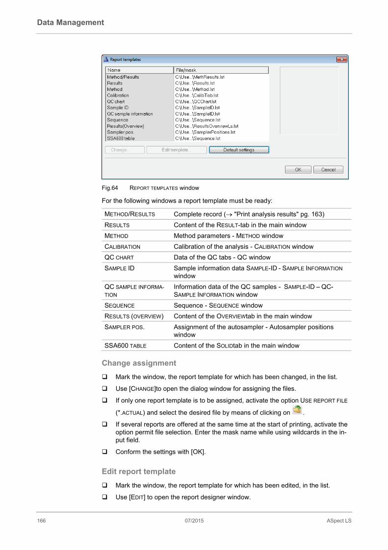
Data Management
166 07/2015 ASpect LS
Fig.64 REPORT TEMPLATES window
For the following windows a report template must be ready:
METHOD/RESULTS Complete record (→ "Print analysis results" pg. 163) RESULTS Content of the RESULT-tab in the main window METHOD Method parameters - METHOD window CALIBRATION Calibration of the analysis - CALIBRATION window QC CHART Data of the QC tabs - QC window SAMPLE ID Sample information data SAMPLE-ID - SAMPLE INFORMATION
window QC SAMPLE INFORMA-TION
Information data of the QC samples - SAMPLE-ID – QC-SAMPLE INFORMATION window
SEQUENCE Sequence - SEQUENCE window RESULTS (OVERVIEW) Content of the OVERVIEWtab in the main window SAMPLER POS. Assignment of the autosampler - Autosampler positions
window SSA600 TABLE Content of the SOLIDtab in the main window
Change assignment Mark the window, the report template for which has been changed, in the list.
Use [CHANGE]to open the dialog window for assigning the files.
If only one report template is to be assigned, activate the option USE REPORT FILE
(*.ACTUAL) and select the desired file by means of clicking on .
If several reports are offered at the same time at the start of printing, activate the option permit file selection. Enter the mask name while using wildcards in the in-put field.
Conform the settings with [OK].
Edit report template Mark the window, the report template for which has been edited, in the list.
Use [EDIT] to open the report designer window.
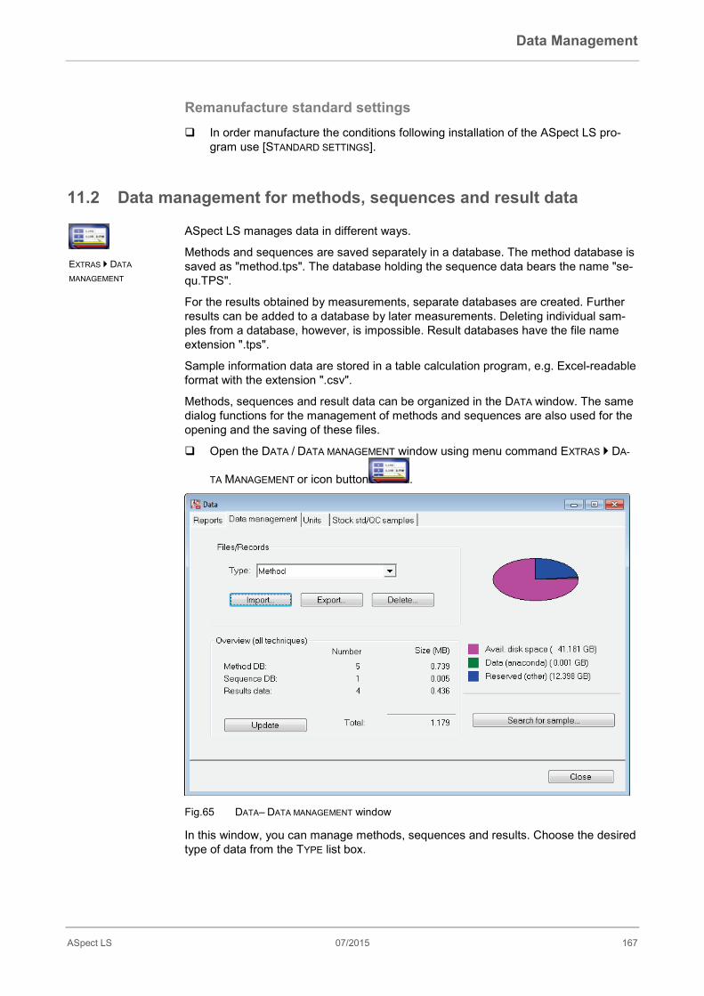
Data Management
ASpect LS 07/2015 167
Remanufacture standard settings In order manufacture the conditions following installation of the ASpect LS pro-
gram use [STANDARD SETTINGS].
11.2 Data management for methods, sequences and result data ASpect LS manages data in different ways.
Methods and sequences are saved separately in a database. The method database is saved as "method.tps". The database holding the sequence data bears the name "se-qu.TPS".
For the results obtained by measurements, separate databases are created. Further results can be added to a database by later measurements. Deleting individual sam-ples from a database, however, is impossible. Result databases have the file name extension ".tps".
Sample information data are stored in a table calculation program, e.g. Excel-readable format with the extension ".csv".
Methods, sequences and result data can be organized in the DATA window. The same dialog functions for the management of methods and sequences are also used for the opening and the saving of these files.
Open the DATA / DATA MANAGEMENT window using menu command EXTRAS DA-
TA MANAGEMENT or icon button .
Fig.65 DATA– DATA MANAGEMENT window
In this window, you can manage methods, sequences and results. Choose the desired type of data from the TYPE list box.
EXTRAS DATA
MANAGEMENT
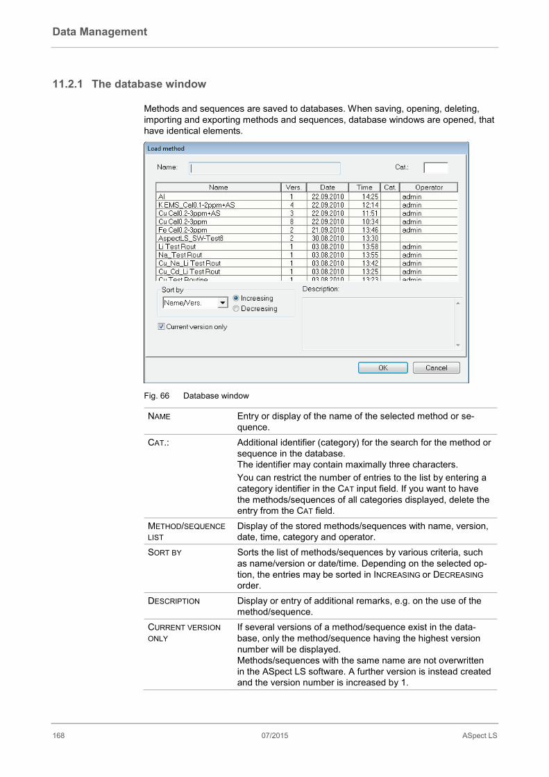
Data Management
168 07/2015 ASpect LS
11.2.1 The database window Methods and sequences are saved to databases. When saving, opening, deleting, importing and exporting methods and sequences, database windows are opened, that have identical elements.
Fig. 66 Database window
NAME Entry or display of the name of the selected method or se-quence.
CAT.: Additional identifier (category) for the search for the method or sequence in the database. The identifier may contain maximally three characters. You can restrict the number of entries to the list by entering a category identifier in the CAT input field. If you want to have the methods/sequences of all categories displayed, delete the entry from the CAT field.
METHOD/SEQUENCE LIST
Display of the stored methods/sequences with name, version, date, time, category and operator.
SORT BY Sorts the list of methods/sequences by various criteria, such as name/version or date/time. Depending on the selected op-tion, the entries may be sorted in INCREASING or DECREASING order.
DESCRIPTION Display or entry of additional remarks, e.g. on the use of the method/sequence.
CURRENT VERSION ONLY
If several versions of a method/sequence exist in the data-base, only the method/sequence having the highest version number will be displayed. Methods/sequences with the same name are not overwritten in the ASpect LS software. A further version is instead created and the version number is increased by 1.
Data Management
ASpect LS 07/2015 169
11.2.2 Managing methods and sequences The databases also provide functions for importing, exporting or deleting individual methods or sequences from the respective databases. In the following, methods and sequences are referred to as data records.
Note
To select several data records of the database window simultaneously, hold the ctrl or shift key depressed.
Open the DATA / DATA MANAGEMENT window using menu command EXTRAS DA-
TA MANAGEMENT or icon button
.
From the TYPE list box, choose the type of data record to be managed: METHOD or SEQUENCE.
Exporting data records Using the export function, you can make data records accessible to other AAS devices of the same type. You may export several data records to a common file. Export files get the following extensions: Method data records - ".met", sequence data records - ".seq".
Click on [EXPORT…] to open the database window.
Select the data sets and click on [EXPORT].
This will bring up the standard SAVE AS... window.
Type in a file name and confirm it with [SAVE].
The database window with the exported files is displayed.
Close the database window with [CLOSE] and return to the DATA window.
Importing data records Using the import function, you can load data records from other AAS devices of the same type into your database. An imported file may contain several data records, from which you can select those to be loaded.
Click on [IMPORT] to open the SELECT FILE FOR IMPORT window with the standard functions for opening files.
Choose the file to be imported.
Confirm the choice with [OPEN].
This will bring up the database window with the presentation of name, date of creation and category of the data records contained in the file. In the title bar of the window, the name of the import file is displayed.
Select the data records to be imported and click on [IMPORT].
The data records are imported into the database. If a method/sequence of the same name should exist already, a new version of the method/sequence will be created. In the database window, the current versions of the available data rec-ords appear.
EXTRAS / DATA
MANAGEMENT
Data Management
170 07/2015 ASpect LS
Close the database window with [CLOSE] and return to the DATA window.
Deleting data records Using the delete function, you can permanently delete data records from the data-base.
Click on [DELETE] to open the database window.
Select the data records to be deleted.
Click on [DELETE]. The database window is being updated displaying only the remaining data rec-ords. With data records of the same name, the version number is kept. The versions will not be renumbered.
Deleting data records via the File menu
Alternatively, you may activate the database windows DELETE METHOD or DELETE SEQUENCE via menu command FILE DELETE METHOD... or FILE DELETE SE-QUENCE....
Then, proceed as described above.
11.2.3 Managing results files Results are always saved to the database during the measurement. A database hold-ing result data may be copied or deleted.
Open the DATA / DATA MANAGEMENT window using menu command EXTRAS DA-
TA MANAGEMENT or icon button .
From the TYPE list box, choose the RESULTS option.
Copying results files With the this command, you may copy one or several databases as well as existing spectrum files to another folder.
Click on [COPY…] to open the COPY RESULTS FILE window with the overview of existing result databases. The results files are listed with name, size and date/time of the last change.
Select the results databases by mouse clicks. To select several databases, keep the ctrl or shift key depressed.
Click on [COPY…] to open the SELECT DIRECTORY window.
Choose the target folder and confirm your choice with [OK].
The results files are being copied to the selected target folder.
Deleting results files Delete the result data permanently.
Select the results database to be deleted by mouse clicks. To select several da-tabases, keep the Ctrl or Shift key depressed.
DATA MANAGEMENT
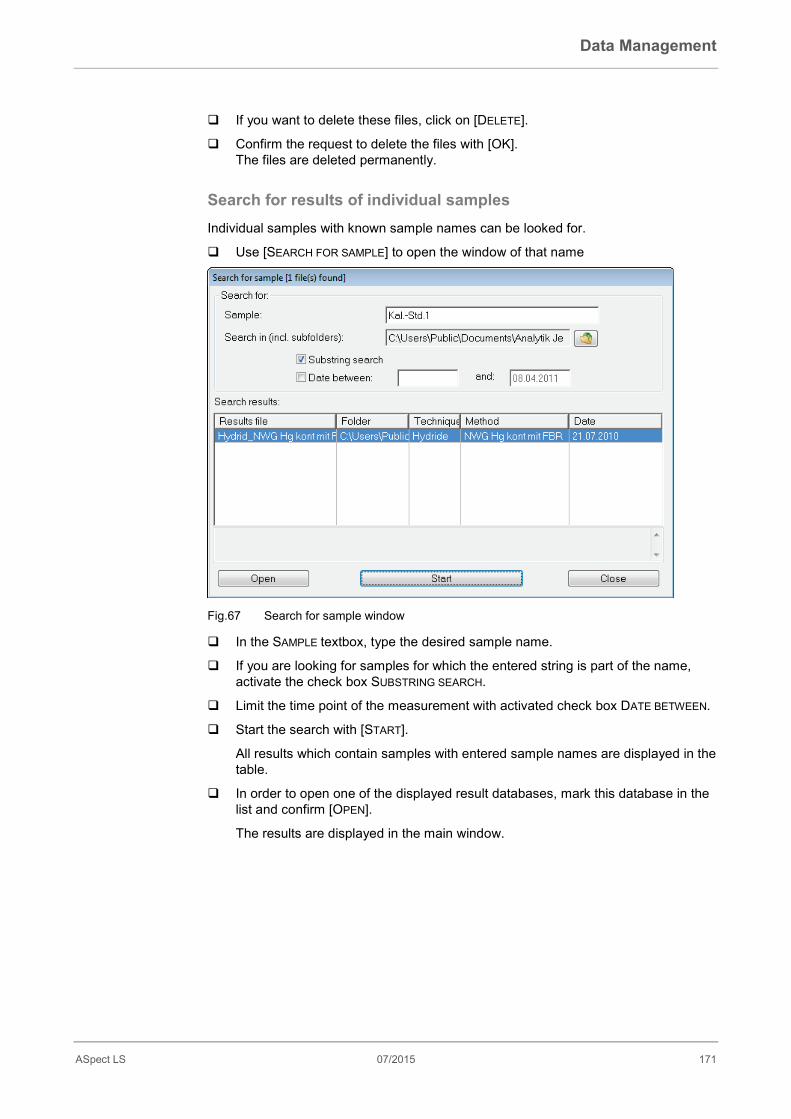
Data Management
ASpect LS 07/2015 171
If you want to delete these files, click on [DELETE].
Confirm the request to delete the files with [OK]. The files are deleted permanently.
Search for results of individual samples Individual samples with known sample names can be looked for.
Use [SEARCH FOR SAMPLE] to open the window of that name
Fig.67 Search for sample window
In the SAMPLE textbox, type the desired sample name.
If you are looking for samples for which the entered string is part of the name, activate the check box SUBSTRING SEARCH.
Limit the time point of the measurement with activated check box DATE BETWEEN.
Start the search with [START].
All results which contain samples with entered sample names are displayed in the table.
In order to open one of the displayed result databases, mark this database in the list and confirm [OPEN].
The results are displayed in the main window.
Data Management
172 07/2015 ASpect LS
11.3 Use Windows-Clipboard
11.3.1 Copying results to the clipboard The application lets you copy the results of selected samples directly to the Windows clipboard thus making them accessible to other Windows applications.
The corresponding commands are contained on the EDIT menu.
COPY VISIBLE COLUMNS ONLY (CTRL+C)
Copies the visible sample results of the current table.
COPY ALL COLUMNS Copies the sample results of all tables. COLUMN TITLES If activated (check mark), the copy action includes
the column headers. Select the samples from the desired table of the results list.
Holding the ctrl or shift key depressed, choose the samples by mouse clicks on the respective row.
To select all rows, use menu command Edit / Select All.
If necessary, activate menu command EDIT / COLUMN TITLES to have the column headers included in the copy action.
Activate the desired menu command to copy the results to the Windows clip-board.
11.3.2 Copying graphics as screenshots You may also copy graphic windows and graphs of calibration curves, absorbance signals or emission signals as screenshots to the Windows clipboard.
Click on the right mouse button on the graph.
A submenu with two copy commands opens.
Select the copy command in order to copy the desired object: only copy the graph or the complete displayed window.
The selected object is copied onto the clipboard and is available for other Win-dows applications.
11.4 Saving results in ASCII/CSV format You may save measurement results both automatically and manually in ASCII/CSV format. For both export formats, the parameters for the decimal and list separator, and the result columns to be exported are to be defined in the OPTIONS - ASCII/CSV EX-PORT window (→ "Export options", pg. 156).
Automatic continuous data export With activated automatic continuous data export option, every entry in the results table is instantly exported to the defined ASCII file. The name of this ASCII file is to be de-fined in the OPTIONS / CONTINUOUS ASCII EXPORT window (→ "Options for continuous ASCII export", pg. 156).
EDIT MENU
CONTINUOUS ASCII-EXPORT TAB

Data Management
ASpect LS 07/2015 173
Manual data export If you intend to export data manually, you can select the rows of the results table to be exported.
Select the samples in the desired results table.
Holding the ctrl or shift key depressed, select the samples by mouse clicks on the respective rows. To select all rows of the table, use menu command EDIT / SELECT ALL.
Then, activate menu command EDIT / SAVE SELECTION to open the SAVE AS standard window for saving files.
Enter the file name and confirm it with [OK]. The data will be saved in the CSV format which can be read by MS Excel and other programs.

User Management
174 07/2015 ASpect LS
12 User Management An optional software package for ASpect LS user management is available. It pro-vides extended functionality for operation of ASpect LS in accordance with the FDA requirements on Electronic Records & Electronic Signatures (21 CFR Part 11).
The user management package allows for one administrator level and four user levels. A user with ASpect LS administrator rights may perform any of the following action with the help of this user management package:
• flexible system configuration (code word and login gidelines, audit trailing, signatures, data directories)
• creation of a user level for each user with a stepped pattern of user rights
• assignment of code words for access to ASpect LS software
• assignment of personalized working directories for methods, sequences and results to users
• inspection and exporting of created audit trail (events log sheet)
Once the user management package is installed and configured, the SYSTEM menu item in ASpect LS will be active. You can use this menu item to access one or more desired functions of user identity management.
Any change in user data will be permanently saved in an encoded data base on exit-ing a pertaining window.
Note
In order to meet safety requirements, a Microsoft Windows operating system with ad-equate configuration resources must be available. This applies to file access rights and other setting actions of a kind that should be performed by an authorized system administrator.
12.1 Hierarchy and access to functions The user identity management package provides for one administrator level and four user levels.
The hierarchy structure for user levels is as follows:
Administrator > level 1> level 2 > level 3 > level 4.
Access to ASpect LS functions
Administrator level
The user has full access rights to ASpect LS and to any function of user identity man-agement.
Level 1
Level 1 users have unlimited access to all ASpect LS functions, but are denied access to user identity management.
Level 2
Same as level 1 users, except:
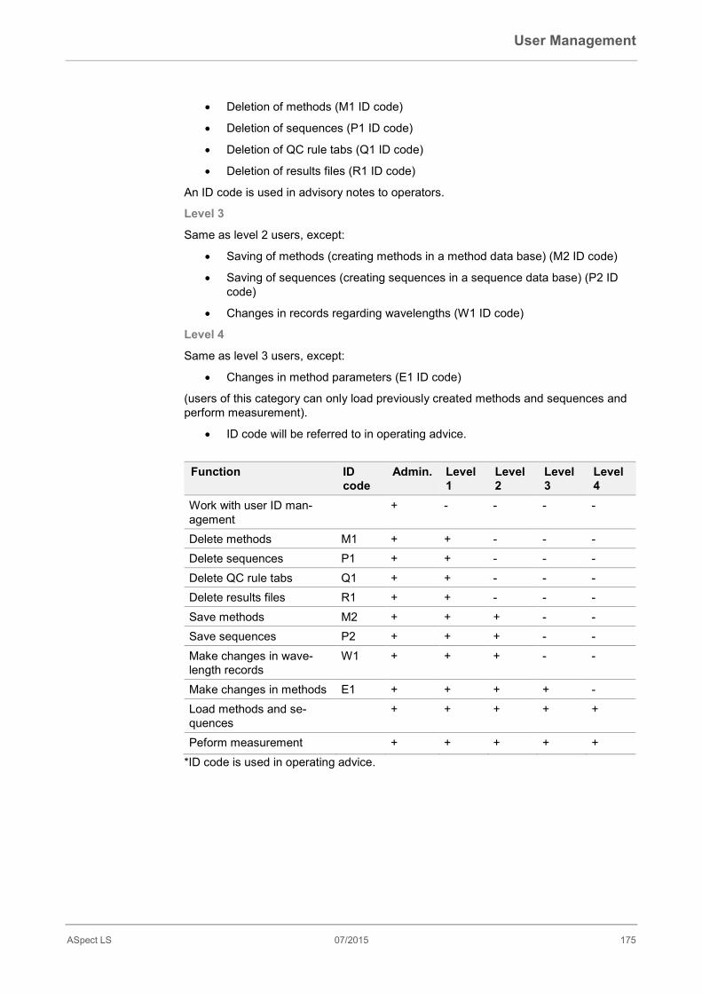
User Management
ASpect LS 07/2015 175
• Deletion of methods (M1 ID code)
• Deletion of sequences (P1 ID code)
• Deletion of QC rule tabs (Q1 ID code)
• Deletion of results files (R1 ID code)
An ID code is used in advisory notes to operators.
Level 3
Same as level 2 users, except:
• Saving of methods (creating methods in a method data base) (M2 ID code)
• Saving of sequences (creating sequences in a sequence data base) (P2 ID code)
• Changes in records regarding wavelengths (W1 ID code)
Level 4
Same as level 3 users, except:
• Changes in method parameters (E1 ID code)
(users of this category can only load previously created methods and sequences and perform measurement).
• ID code will be referred to in operating advice.
Function ID
code Admin. Level
1 Level 2
Level 3
Level 4
Work with user ID man-agement
+ - - - -
Delete methods M1 + + - - - Delete sequences P1 + + - - - Delete QC rule tabs Q1 + + - - - Delete results files R1 + + - - - Save methods M2 + + + - - Save sequences P2 + + + - - Make changes in wave-length records
W1 + + + - -
Make changes in methods E1 + + + + - Load methods and se-quences
+ + + + +
Peform measurement + + + + + *ID code is used in operating advice.

User Management
176 07/2015 ASpect LS
12.2 User Management setups User management setups can be made by an ASpect LS user with administrator rights as part of initial installation of the user ID management software package or at any time thereafter.
A so-called account is created for each user. An account contains a given user profile. Where a user account is not required any longer, it can be disabled or inhibited. User accounts cannot be deleted.
Trigger a SYSTEM USER MANAGEMENT menu command or launch user manage-ment via an entry button of this name in the starting menu.
On completion of login procedures, the USER MANAGEMENT window will open.
Fig. 68 USER MANAGEMENT window
The window contains a list of registered user names with assigned passwords. It shows the user profile details for a selected user in its right-hand subarea.
Indicator and control elements
USERID Login name of user USER Administrator, level 1 to level 4 E-SIGNATURE YES: User is authorized to electronically sign result data.
NO: User has no authorization for electronic signature. STATUS ACTIVE: User name allowed for use (green circle).
DISABLED: User name was disabled and cannot be used (red cir-cle).
PASSWORD PRO-TECTION
ACTIVE: User login requires a code word (key) INACTIVE: User login allowed without a code word (key crossed
out) VALID UNTIL UNLIMITED: Password never expires.
DATE/DAYS: User must change his/her password on expiry of specified term.
SYSTEM USER
MANAGMENT
User Management
ASpect LS 07/2015 177
FULL NAME Complete name of user DESCRIPTION Optional description of user
Control buttons
[NEW ...] Creates new user. Opens the ADD USER DATA window.
[MODIFY ...] Changes user data for a marked table line. The MODIFY USER DATA window will open for a marked table line. The same dialog screen may be called up by double-clicking the particular table line.
[PREFERENCES...] Allows changes in user management configuration.
[AUDIT TRAIL.... Audit trail (events logsheet)
[EXIT] Terminates this application.
12.2.1 Configuring user management For configuration, the PREFERENCES window provides selection options as follows:
• Password policies
• Login and audit trail
• Signature meanings
• Selected data directories
Click onto [Preferences...] in ASpect LS User Management window.
The PREFERENCES window opens.
Select an option group you want to change from the left column.
These setups will be valid for newly created user accounts. They should therefore be made following installation. On exiting the window with [OK], all setups will be saved, on selection of [CANCEL], they modified settings will be discarded.
[SET DEFAULT SETTINGS]
Sets the default settings (factory settings) for a given selection. The settings for other areas will be unaffected.
User Management
178 07/2015 ASpect LS
Login/password
Fig. 69 Setups for login and password policies
Login policies (for new user names)
NUMBER OF LOGIN AT-TEMPTS
Shows the number of invalid login attempts (max. 10). On excession of the maximum allowed number, the ASpect LS session will be terminated after a cetrain waiting time and must be restarted for another login. An entry (warning) is added to the audit trail file.
MINIMUM USER NAME LENGTH
Defines the minimum prescribed number of characters for a newly created user name Maximum number of characters: 10
Password policies (for new user names)
ENFORCE LOGIN WITH PASSWORD
A password must be assigned to newly created user names.
PASSWORD WITH LETTERS AND NUM-BERS
Only passwords consisting of letters and numeric characters can be assigned. This policy equally applies to changes in password.
PASWORD AND US-ER ID MUST BE DIF-FERENT
Only passwords which are different from the respective user name will be accepted. This policy equally applies to changes in password.
"USER MUST CHANGE ASSWORD AT NEXT LOGON!" IS ACTIVE
For newly created users, the CHANGE PASSWORD AT NEXT LO-GON!checkbox will be turned on by default. The user will be prompted to change his/her password when logging in to AS-pect LS for the next time.
User Management
ASpect LS 07/2015 179
PASSWORD EX-PIRES IN ...DAY(S)
On expiry of a preset term, the user will be prompted to change his/her password when logging in to ASpect LS. The password is then extended by a term as set in Policies. This value is then acknowledged as a template that can be modified for other sin-gle users (max. 999 days).
MINIMUM LENGTH OF PASSWORD
Designates the minimum required number of characters for a newly created password; number of characters: 3 to 10
Fig. 70 Setups for paths
The Aspect LS working directory and the audit trail directory provide specification op-tions.
Paths
ASPECT-WORKING DIREC-TORY
Working directory of ASpect LS. The working directory contains a data base of methods and se-quences and results files. The working directory was defined as part of ASpect LS installation and may be changed at this point.
AUDIT TRAIL Path of audit trail file. This path may be changed.
USER DATABASE Path of user data base. This path may only be changed with the help of the installation program.

User Management
180 07/2015 ASpect LS
Audit Trail
Fig. 71 Settings for audit trail data
INACTIVE (NO ENT-RIES)
No entries will be added to the audit trail file (event log sheet).
ACTIVE Entries will be added to the audit trail file (event log sheet). ALLOW MEASURING ONLY WITH SAVED METHODS
When active, this checkbox allows a measurement to be trig-gered in ASpect LS only if a method was loaded and no change was made in this method since it was saved for the last time.

User Management
ASpect LS 07/2015 181
Signatures
Fig. 72 Editing of signature meanings
This list shows those signature meanings that are selectable for signing.
ADD Adds a signature meaning, e.g. created, reviewed, approved (max. 30 characters).
MODIFY Changes a signature meaning that was marked in the list. DELETE Deletes a signature meaning that was marked in the list.
12.2.2 Creating a new user account Only users with administrator access rights are authorized to create a new user ac-count.
Click the [NEW] button in the USER MANAGEMENT window, in order to create a new user account.
The ADD USER DATA window appears.

User Management
182 07/2015 ASpect LS
Fig. 73 Editing of user data
The input fields in this window provide setting options as follows:
USER ID The name that is required for a user to log in. No checks are made for capital and small lettering. The min-imum name length depends on configuration settings made in LOGIN/PASSWORD (→ "Configuring user management" p. 177 et seq.). Max. length: 32 characters
FULL NAME Full name of user. This name will serve as a constituent of the electronic signature. Max. length: 30 characters
DESCRIPTION A field for note or comment text. Entry is optional. USER LEVEL User level PASSWORD... Opens a dialog screen for password entry.
Max. password length: 20 characters The minimum length and other password policy rules may be configured (→ "Configuring user management" p. 177 et seq.). Capital lettering and small lettering are distinguished for passwords. If the password dialog is acknowledged without a password entry, the password protection will be canceled. KEY icon:
Password protection is active. KEY CROSSED OUT icon:
User name uses no password. PASSWORD NEVER EXPIRES
Password will remain valid for unlimited time if this box is ac-tive. If it was disabled, the given password will expire within a pre-set term.

User Management
ASpect LS 07/2015 183
The specified value is sourced from password policies. A us-er may also extend his/her password in advance.
USER-SPECIFIC DATA PATH
If active, this box will create the user’s own working directory in this format: \ASpect-Working directory\User name. As part of an initial login to ASpect LS the appropriate direc-tory structure will be created.
USE E-SIGNATURE Allows the user to electronically sign for measured results if active.
DISABLE USER ID Prohibits the use of a user name if active. User names can be temporarily disabled. A disabled (as op-posed to a removed) user name cannot be reassigned to an-other newly created user.
USER MUST CHANGE PASSWORD AT NEXT LOGON
Will prompt the user to change his/her password as the next ASpect LS session is triggered.
Click [OK] to confirm all features of a newly created user account.
12.2.3 Modifying a previously created user account To select a user account you want to modify, click this account in the table of the
User Management dialog window, then click the [Modify] button.
The EDIT USER DATA window with selected accounts will open (→ "Creating a new user account" p. 181).
12.3 Viewing and exporting Audit Trail An audit trail file keeps track of certain system events and any warning or error mes-sage that occurred during an ASpect LS session.
Click [AUDIT TRAIL...] in the User Management window
or:
Select the SYSTEM / AUDIT TRAILmenu command in ASpect LS.
The audit trail can now be:
• viewed
• updated
• copied for backup purposes before final deletion (only if Audit Trail was called up from the USER MANAGEMENT window)
• exported as a "*.csv" file (only if Audit Trail was called up from the USER MAN-AGEMENT window)
SYSTEM / AUDIT
TRAIL
User Management
184 07/2015 ASpect LS
Fig. 74 AUDIT TRAIL window selected in USER MANAGEMENT window
The following parameters are documented in an audit trail file:
TYPE Indicates the type of an event An audit trail keeps track of the following types of events and marks these with symbols: INFO, WARNING, ERROR, LOGIN and LOGOUT
DATE/TIME Designates the date and exact time of an entry (PC watch) TIME ZONE Indicates the time zone to which the time of an entry is referenced
(Windows system control) NAME Describes an event, for details refer to DESCRIPTION field:
LOGIN: Logs in LOGOUT/EXIT: Terminates an application ADD/CHANGE/DELETE: Edits methods, sequences and user data PWDCHG: Allows changes in password RUN: Triggers an analytical sequence PRINT: Prints trailer file SIGN: For signing of results #nnnn: Error number
CAT. Shows the category of an event. "USRMGMNT" is the category used to mark those entries made in User Management. All other categories will be entered by ASpect LS.
OPERATOR Designates the user in login state at the moment of an entry. DESCRIPTION Provides more detail about the cause of an entry.
Updating an audit trail You may use [REFRESH] to update the list of entries in an audit trail.
This may be necessary if further entries were added to a previously created audit trail display.
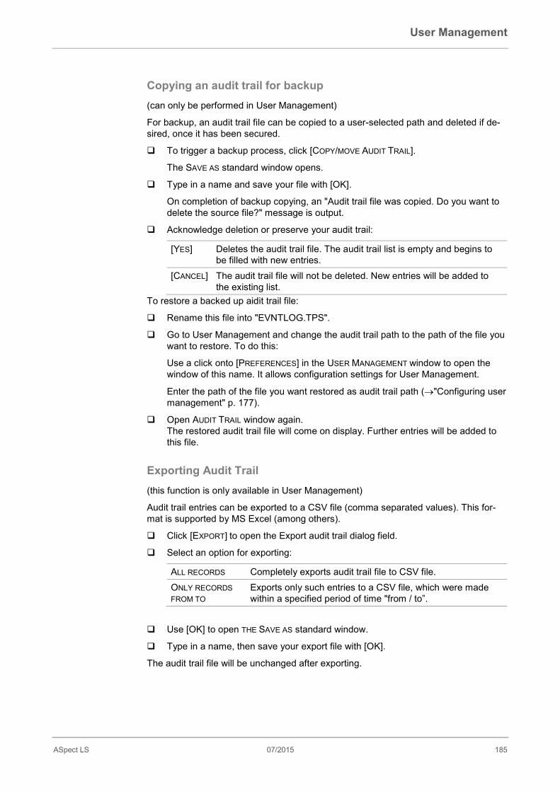
User Management
ASpect LS 07/2015 185
Copying an audit trail for backup (can only be performed in User Management)
For backup, an audit trail file can be copied to a user-selected path and deleted if de-sired, once it has been secured.
To trigger a backup process, click [COPY/MOVE AUDIT TRAIL].
The SAVE AS standard window opens.
Type in a name and save your file with [OK].
On completion of backup copying, an "Audit trail file was copied. Do you want to delete the source file?" message is output.
Acknowledge deletion or preserve your audit trail:
[YES] Deletes the audit trail file. The audit trail list is empty and begins to be filled with new entries.
[CANCEL] The audit trail file will not be deleted. New entries will be added to the existing list.
To restore a backed up aidit trail file:
Rename this file into "EVNTLOG.TPS".
Go to User Management and change the audit trail path to the path of the file you want to restore. To do this:
Use a click onto [PREFERENCES] in the USER MANAGEMENT window to open the window of this name. It allows configuration settings for User Management.
Enter the path of the file you want restored as audit trail path (→"Configuring user management" p. 177).
Open AUDIT TRAIL window again. The restored audit trail file will come on display. Further entries will be added to this file.
Exporting Audit Trail (this function is only available in User Management)
Audit trail entries can be exported to a CSV file (comma separated values). This for-mat is supported by MS Excel (among others).
Click [EXPORT] to open the Export audit trail dialog field.
Select an option for exporting:
ALL RECORDS Completely exports audit trail file to CSV file. ONLY RECORDS FROM TO
Exports only such entries to a CSV file, which were made within a specified period of time "from / to”.
Use [OK] to open THE SAVE AS standard window.
Type in a name, then save your export file with [OK].
The audit trail file will be unchanged after exporting.

User Management
186 07/2015 ASpect LS
12.4 Changing a password Depending on his/her user account settings, a user may or may have to change his/her password at regular intervals.
Select the SYSTEM CHANGE PASSWORD menu command in ASpect LS.
The CHANGE PASSWORD dialog screen opens.
Enter your previous password at the input field, then enter the new password twice and click [OK].
On successful entry, a "Password changed" message will appear.
12.5 Electronic signatures ASpect LS allows users to electronically sign up for their result data provided the given user has authorization to USE E-SIGNATURE (→ "Creating a new user account" p. 181). A signature will close work on a particular file so changes in this file made at a later point in time will cause an invalid signature state.
A sign-up procedure will encode a given file and assign to this file a signed state and the data of the signing user. In addition, an encoded signature file of identical name (same as results file) will be created, except that this signature file carries a *.sig data extention. It contains the checksums of the related results file, including those of (if included) a spectrum file.
A file may be signed by more than one user.
12.5.1.1 Signing measured results A file of measured results may be sealed with an electronic signature by one or more users authorized to do so on completion of measurement or when this file is loaded at some later point in time.
Select the SYSTEM SIGN OFF RESULTS menu command in ASpect LS.
The SIGN OFF dialog screen opens.
USER ID The login name of a current user. A user ID may be modified to facilitate signing by more users (max. 32 characters).
PASSWORD Code word of a user (max. 20 characters). MEANING The measning of a signature, for example, Created, Reviewed,
Approved. To define a list of signature meanings is the responsibility of the User Management administrator (→ "Configuring user manage-ment" p. 177).
COMMENT For optional comment (max. 256 characters) [SIGN OFF] Signs a given document with any settings it contains.
After actuation of [SIGN OFF], you will be asked if this signature is granted or if the process is to be aborted. Successful granting of a signature will be confirmed.
SYSTEM CHANGE
PASSWORD
SYSTEM SIGN OFF
RESULTS
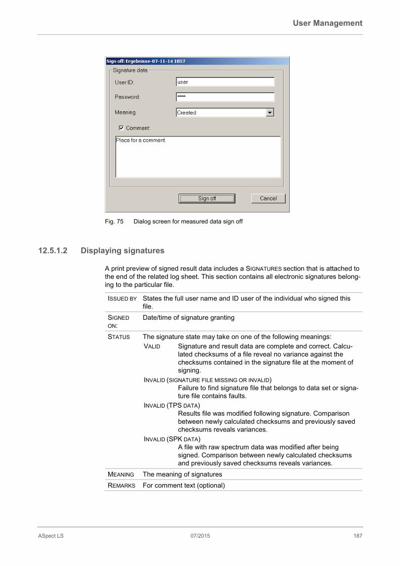
User Management
ASpect LS 07/2015 187
Fig. 75 Dialog screen for measured data sign off
12.5.1.2 Displaying signatures A print preview of signed result data includes a SIGNATURES section that is attached to the end of the related log sheet. This section contains all electronic signatures belong-ing to the particular file.
ISSUED BY States the full user name and ID user of the individual who signed this file.
SIGNED ON:
Date/time of signature granting
STATUS The signature state may take on one of the following meanings: VALID Signature and result data are complete and correct. Calcu-
lated checksums of a file reveal no variance against the checksums contained in the signature file at the moment of signing.
INVALID (SIGNATURE FILE MISSING OR INVALID) Failure to find signature file that belongs to data set or signa-ture file contains faults.
INVALID (TPS DATA) Results file was modified following signature. Comparison between newly calculated checksums and previously saved checksums reveals variances.
INVALID (SPK DATA) A file with raw spectrum data was modified after being signed. Comparison between newly calculated checksums and previously saved checksums reveals variances.
MEANING The meaning of signatures REMARKS For comment text (optional)

Supplement / Overview of markings used in the display of values
188 07/2015 ASpect LS
13 Supplement / Overview of markings used in the display of values
Remark Meaning Values Output > Cal The mean value is larger than the
working range of the calibration curve. Mean val-ues
Sequence and results window
< Cal The mean value is smaller than the working range of the calibration curve.
Mean val-ues
Sequence and results window
< LOD The value is smaller than the limit of detection.
Mean val-ues
Sequence and results window
< LOQ The value is smaller than the limit of quantitation and larger than the limit of detection.
Mean val-ues
Sequence and results window
RSD! The mean value is outside the range of the specified relative standard devia-tion.
Mean val-ues
Sequence and results window
RR! The mean value is outside the range of the specified relative range.
Mean val-ues
Sequence and results window
Factor! Limit of recalibration factor for the cali-bration curve was exceeded
Calibration curve
Sequence and results window
R2(adj.) The quality of regression R2(adj.) of the calibration curve falls below the specified value.
Calibration curve
Sequence and results window Calibration curve window
#MAN. The value was manually excluded from the calculation of the mean value.
Single val-ues
Sample individu-al values window
#COR. The value was automatically excluded from the calculation of mean values by the Grubbs outlier test
Single val-ues
Sample individu-al values window

Index
ASpectLS-V13-Deu Index • 189
14 Index
A
Adjust autosampler AS 51/52s 118
Ashing 99
Atomize 99
Autosampler
graphite tube technique 27
Solid analytics 29
Autosampler AS 51/52s
Dosing speed 115
Insertion depth 115
Autosampler MPE 60
Adjustment 128
Depth adjustment 124
Dosing speed 124
Insertion depth 124
Autosampler SSA 600
Depth adjustment 124
Autosampler window 112, 120
Autosamplers
Flame technique 25
Hydride and HydrEA techniques. 25
Autozero 99
Auto-Zero 99
B
Baking (cleaning) of graphite tube 107
Burner
Control functions 91
Buttons
generally used 4
C
Calibration
Delete Standard 76
calibration curve
Newly determine 77
Calibration curve
Display 74
Residual tab 76
Calibration table
Automatic preparation 36
Manual preparation 35
Clean 99
Cleaning
controlled 26, 28
Cookbook 141
D
Depth correction
MPE 60 123
Dosing speed
MPE 60 123
E
Enrichment 100
F
Flame
Automatic optimization 95
Extinguish 97
Set 91
Flame window 91
Function keys 5
Furnace program
Graphic 105
Trial run 105
Furnace Program
Edit 97
Furnace window 97
G
Graphite tube
Service life 107
Graphite tube
Coating 105
Graphite tube
Sensor error 108
Index
190 07/2015 ASpect LS
Graphite tube furnace
Format 107
Graphs 5
H
Hydride system
Heat cell 110
Initialize 108
Loading 108
Rinsing 109
Hydride system window 108
I Injection step 100
L
Limit of detection 77
Limit of quantitation 76
Limit of quantitation 77
Limits of detection and quantitation 76
M
Main Settings
Solid Analysis 8
Solution Analysis 8
Main window 61
Results tab 62
Sequence/Results tab 61
Manual flame optimization 94
Menu command
System Sign off results 164
Menu command ?
Help Topics 3
Menu command Edit
Column titles 152
Column Titles 152
Copy 4, 55
Copy all columns 152
Copy visible columns only (Ctrl+C) 152
Insert 4, 55
Save selection... 153
Select All 152, 153
Menu command Extras
Data Management 143, 147, 149
Data management... 139
Options 134
Menu command file
Open Sample Information File... 53
Menu command File
Delete / Method... 150
Delete / Sequence... 150
Exit 2
Main Settings 7
New Method 12
New Sample Information File 52
New Sequence... 46
Open method... 13
Open results 61
Open Sequence .... 47
Print / Active Window... 144, 145
Print / Report 143
Printer Setup… 5
Report design mode 145
Save / Method 13
Save / Sample Information 52
Save / Sequence 46
Start Offline 60
Menu command method development
Furnace... 97
Menu command Method Development
Flame... 91
Hydride... 108
Method 12
QC... 78
Sample ID 52
Sequence 46
Spectrometer... 82
Index
ASpectLS-V13-Deu Index • 191
Menu Command method development
calibration... 74
Menu command Routine
Break 59
Continue 59
Extinguish flame 97
Reprocess 77
Reprocess... 60
Run Selected Sequence Row... 59
Start Sequence 58
Stop 59
Menu command System
Audit Trail 161
Change Password 163
Menu command System: 155
Menu command View
Close Display Windows 58
Detail results 66
Update result list 61
Menu Command View
Open Display Windows 58
Method development
Cookbook 142
Method development menu command
Autosampler... 112, 120, 130
MPE 60 autosampler
Align to graphite tube 126
O
Offline mode 2
P
Pyrolyse 99
R
Result window
Sequence tab 62
Solid tab 66
User defined tab 65
Results window
Table overview 66
S
Sample ID 54
Sample ID window 54
Single values 67
Single values window 66
Solid autosampler window 130
Spectrometer window 82
Stock standard
Save in database 140
Stock standards
define manually 36
T
Tables
Adjusting 4
Marking 4
Temperature-time program 97
Thermal furnace overheating 99
Thermal pretreatment 100
U
User management
Account 155
User Management
Hierarchy 154
User profile 156
W
Washing
AS 52s 26
MPE 60 29
Window
cookbook 141
Main Settings 7
Peak search 85
search for sample 151