The Spillover Effects of a Downturn in China’s Real Estate Investment

Ashvin Ahuja and Alla Myrvoda

WP/12/266

© 2012 International Monetary Fund WP/12/266

IMF Working Paper

Asia and Pacific Department

The Spillover Effects of a Downturn in China’s Real Estate Investment

Prepared by Ashvin Ahuja and Alla Myrvoda1

Authorized for distribution by Steve Barnett

November 2012

Abstract

Real estate investment accounts for a quarter of total fixed asset investment (FAI) in China. The real estate sector’s extensive industrial and financial linkages make it a special type of economic activity, especially where the credit creation process relies primarily on collateral, like in China. As a result, the impact on economic activity of a collapse in real estate investment in China—though a low-probability event—would be sizable, with large spillovers to a number of China’s trading partners. Using a two-region factor-augmented vector autoregression model that allows for interaction between China and the rest of the G20 economies, we find that a 1-percent decline in China’s real estate investment would shave about 0.1 percent off China’s real GDP within the first year, with negative spillover impacts to China’s G20 trading partners that would cause global output to decline by roughly 0.05 percent from baseline. Japan, Korea, and Germany would be among the hardest hit. In that event, commodity prices, especially metal prices, could fall by as much as 0.8–2.2 percent below baseline one year after the shock.

JEL Classification Numbers: E22, F62, O57

Keywords: China, Investment, Real estate investment, Spillovers, FAVAR

Author’s E-Mail Address: aahuja@imf.org

1The authors thank the following people for their useful comments: Steven Barnett, II Houng Lee, Andre Meier, Malhar Nabar, Papa N’Diaye, other participants at the spillover task force workshop held at the IMF in May 2012, as well as the seminars held at the People’s Bank of China and the National Development and Reform Commission in Beijing, China, in June 2012.

This Working Paper should not be reported as representing the views of the IMF. The views expressed in this Working Paper are those of the author(s) and do not necessarily represent those of the IMF or IMF policy. Working Papers describe research in progress by the author(s) and are published to elicit comments and to further debate.

2

Contents Page

I. Introduction ............................................................................................................................3  II. Modeling the Spillover Effects .............................................................................................4  III. Domestic Feedback ..............................................................................................................6  IV. Global Spillover ...................................................................................................................9  V. Conclusion ..........................................................................................................................13 

References ................................................................................................................................14 

Appendix A: The China–G20 Macro Financial FAVAR……………………………………………….15

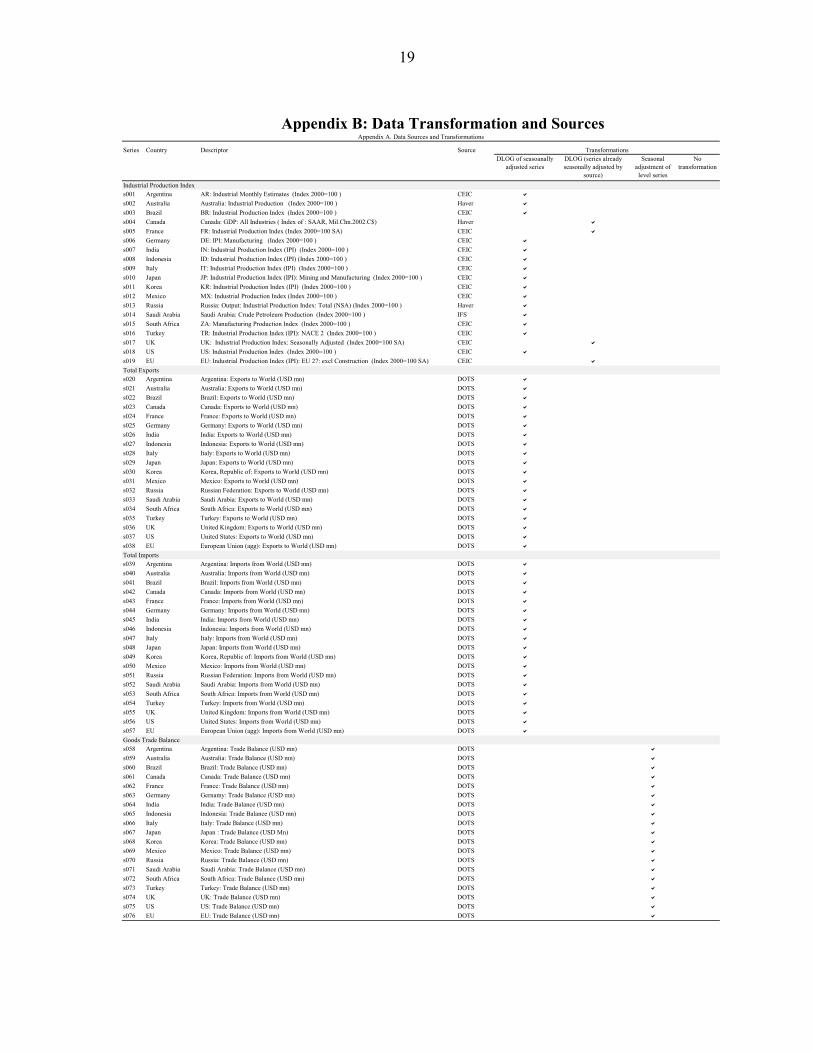
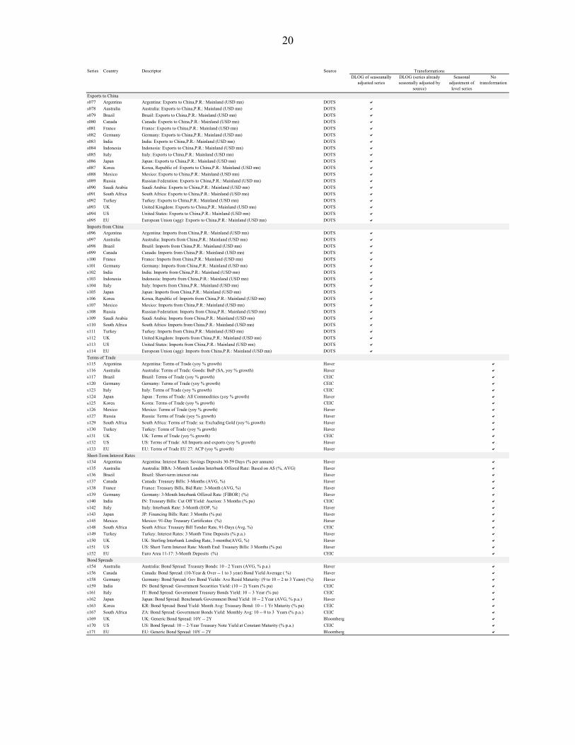
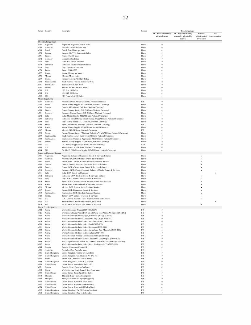
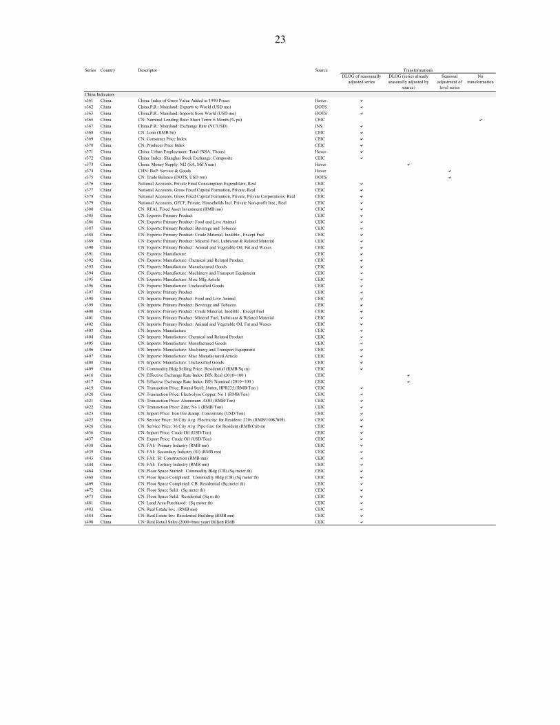
B: Data Transformation and Sources………………………………………………………..19 

3

-50

-25

0

25

50

75

100

2001 2001 2002 2003 2004 2005 2006 2007 2008 2009 2010 2011 2012

Real Estate Investment

Residential Property Price

Property Price and Real Estate Investment(In percent, year-on-year growth)

Primary industry (2%)

Mining (4%)

Manufacturing (34%)

Utilities (5%)

Real estate (25%)

Other (30%)

Fixed Asset Investment: by Industry(In percent of total, 2011)

Source: CEIC

I. INTRODUCTION

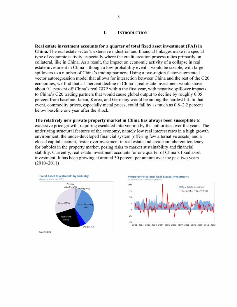
Real estate investment accounts for a quarter of total fixed asset investment (FAI) in China. The real estate sector’s extensive industrial and financial linkages make it a special type of economic activity, especially where the credit creation process relies primarily on collateral, like in China. As a result, the impact on economic activity of a collapse in real estate investment in China—though a low-probability event—would be sizable, with large spillovers to a number of China’s trading partners. Using a two-region factor-augmented vector autoregression model that allows for interaction between China and the rest of the G20 economies, we find that a 1-percent decline in China’s real estate investment would shave about 0.1 percent off China’s real GDP within the first year, with negative spillover impacts to China’s G20 trading partners that would cause global output to decline by roughly 0.05 percent from baseline. Japan, Korea, and Germany would be among the hardest hit. In that event, commodity prices, especially metal prices, could fall by as much as 0.8–2.2 percent below baseline one year after the shock.

The relatively new private property market in China has always been susceptible to excessive price growth, requiring escalated intervention by the authorities over the years. The underlying structural features of the economy, namely low real interest rates in a high growth environment, the under-developed financial system (offering few alternative assets) and a closed capital account, foster overinvestment in real estate and create an inherent tendency for bubbles in the property market, posing risks to market sustainability and financial stability. Currently, real estate investment accounts for one quarter of China’s fixed asset investment. It has been growing at around 30 percent per annum over the past two years (2010–2011)

4

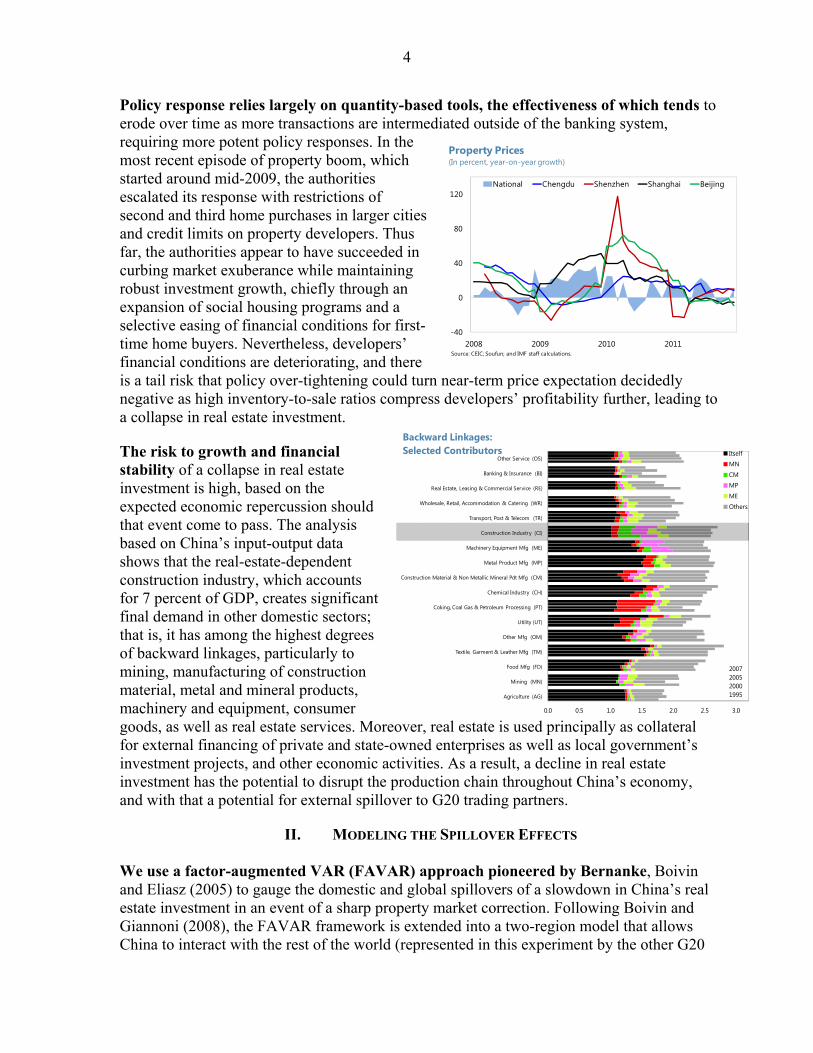
Policy response relies largely on quantity-based tools, the effectiveness of which tends to erode over time as more transactions are intermediated outside of the banking system, requiring more potent policy responses. In the most recent episode of property boom, which started around mid-2009, the authorities escalated its response with restrictions of second and third home purchases in larger cities and credit limits on property developers. Thus far, the authorities appear to have succeeded in curbing market exuberance while maintaining robust investment growth, chiefly through an expansion of social housing programs and a selective easing of financial conditions for first-time home buyers. Nevertheless, developers’ financial conditions are deteriorating, and there is a tail risk that policy over-tightening could turn near-term price expectation decidedly negative as high inventory-to-sale ratios compress developers’ profitability further, leading to a collapse in real estate investment.

The risk to growth and financial stability of a collapse in real estate investment is high, based on the expected economic repercussion should that event come to pass. The analysis based on China’s input-output data shows that the real-estate-dependent construction industry, which accounts for 7 percent of GDP, creates significant final demand in other domestic sectors; that is, it has among the highest degrees of backward linkages, particularly to mining, manufacturing of construction material, metal and mineral products, machinery and equipment, consumer goods, as well as real estate services. Moreover, real estate is used principally as collateral for external financing of private and state-owned enterprises as well as local government’s investment projects, and other economic activities. As a result, a decline in real estate investment has the potential to disrupt the production chain throughout China’s economy, and with that a potential for external spillover to G20 trading partners.

II. MODELING THE SPILLOVER EFFECTS We use a factor-augmented VAR (FAVAR) approach pioneered by Bernanke, Boivin and Eliasz (2005) to gauge the domestic and global spillovers of a slowdown in China’s real estate investment in an event of a sharp property market correction. Following Boivin and Giannoni (2008), the FAVAR framework is extended into a two-region model that allows China to interact with the rest of the world (represented in this experiment by the other G20

-40

0

40

80

120

2008 2009 2010 2011

National Chengdu Shenzhen Shanghai Beijing

Property Prices(In percent, year-on-year growth)

Source: CEIC; Soufun; and IMF staff calculations.

0.0 0.5 1.0 1.5 2.0 2.5 3.0

Agriculture (AG)

Mining (MN)

Food Mfg (FD)

Textile, Garment & Leather Mfg (TM)

Other Mfg (OM)

Utility (UT)

Coking, Coal Gas & Petroleum Processing (PT)

Chemical Industry (CH)

Construction Material & Non Metallic Mineral Pdt Mfg (CM)

Metal Product Mfg (MP)

Machinery Equipment Mfg (ME)

Construction Industry (CI)

Transport, Post & Telecom (TR)

Wholesale, Retail, Accommodation & Catering (WR)

Real Estate, Leasing & Commercial Service (RE)

Banking & Insurance (BI)

Other Service (OS)ItselfMN

CMMP

MEOthers

Backward Linkages: Selected Contributors

2007200520001995

5

economies). The analysis captures the feedback from China to the rest of the world, and vice versa, over time. It also captures the spillover effect between the rest of the G20 economies from a specific event originated in China.

The fact that market participants monitor hundreds of economic variables in their decision making process provides motivation for conditioning the analysis of their decisions on a rich information set. The FAVAR framework extracts information from the rich data set to gauge the impact of particular forces that may not be directly observable. These “forces” are treated as latent common components, which are inter-related, and their impacts on economic variables are traced through impulse response functions. By accounting for unobserved variables, there is a better chance that findings based on spurious association can be avoided.

More detailed description of the model and estimation strategy can be found in the appendix. Briefly, the model is a stable FAVAR in growth (except for balances and interest rates) with 5 common factors for each region (China and the rest of the G20 economies) and China’s real estate investment. The model uses one lag. The Cholesky factor from the residual covariance matrix is used to orthogonalize the impulses, which imposes an ordering of the variables in the VAR and treats real estate investment as exogenous in the period of shock. The results are robust to re-ordering within factor groups. The data set is a balanced panel of 390 monthly time series from the G20 stretching from 2000M1 to 2011M9, with 68 China’s variables and 322 from the rest of the world (see data description, transformation, and sources in Appendix B). Our sample contains at least one full cycle of real estate investment and property market in China. It covers the period when China entered the WTO and became increasingly integrated with the world economy.

Since the model is in growth, the experiment assumes an exogenous, temporary, one-standard-deviation growth shock to China’s real estate investment. The shock dampens within a few months and dissipates fully after around 36 months. Specifically, this is a one-time 49-percentage-point (seasonally adjusted, annualized) drop in real estate investment growth that reverts to trend growth largely within 4–5 months.2 While this is a temporary, negative growth shock, the decline in real estate investment level is permanent. The shock is approximately equivalent to a 2-percent drop from baseline in real estate investment level 12 months after. The analysis does not assume policy response beyond that which was already in the sample.

2 One standard deviation shock is equivalent to 3 percentage points in month-over-month, seasonally adjusted, growth rates.

6

-8

-6

-4

-2

0Significant

Not significant

China: Peak Impact on Exports and Imports(In percentage points, saar; 1 s.d. shock)

Primaryproducts

Mineralfuel,

lubricants

Manufacturing Chemical Products

Manufac-tured goods

Machinery&

transport

Manufacturing Exports

Exports Imports

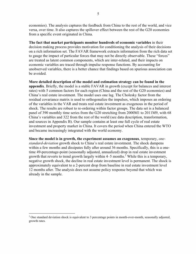
Twenty-four-month peak impacts to one-standard-deviation shock to real estate investment are reported with standard error bands in the charts below. Impacts on levels 12 months after the shock, in percent below baseline, are also derived and reported for comparison in Tables 1–4.

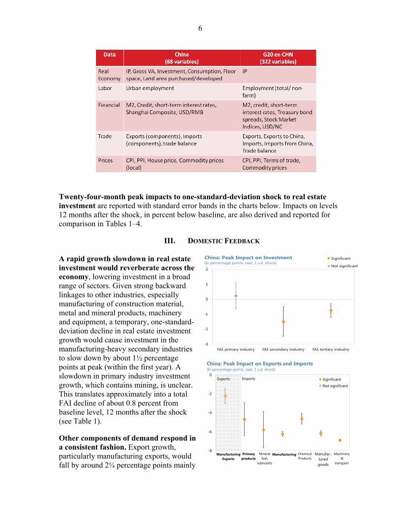
III. DOMESTIC FEEDBACK A rapid growth slowdown in real estate investment would reverberate across the economy, lowering investment in a broad range of sectors. Given strong backward linkages to other industries, especially manufacturing of construction material, metal and mineral products, machinery and equipment, a temporary, one-standard-deviation decline in real estate investment growth would cause investment in the manufacturing-heavy secondary industries to slow down by about 1½ percentage points at peak (within the first year). A slowdown in primary industry investment growth, which contains mining, is unclear. This translates approximately into a total FAI decline of about 0.8 percent from baseline level, 12 months after the shock (see Table 1).

Other components of demand respond in a consistent fashion. Export growth, particularly manufacturing exports, would fall by around 2¼ percentage points mainly

-3

-2

-1

0

1

2

FAI: primary industry FAI: secondary industry FAI: tertiary industry

Significant

Not significant

China: Peak Impact on Investment(In percentage points, saar; 1 s.d. shock)

7

-10

-8

-6

-4

-2

0

-10

-8

-6

-4

-2

0

Significant

Not significant

China: Peak Impact on Macroeconomic Indicators(In percentage points, saar; 1 s.d. shock)

Gross value added index

Real retailsales

Exports Imports Urban employment

CPIinflation

Shanghai Stock Exchange

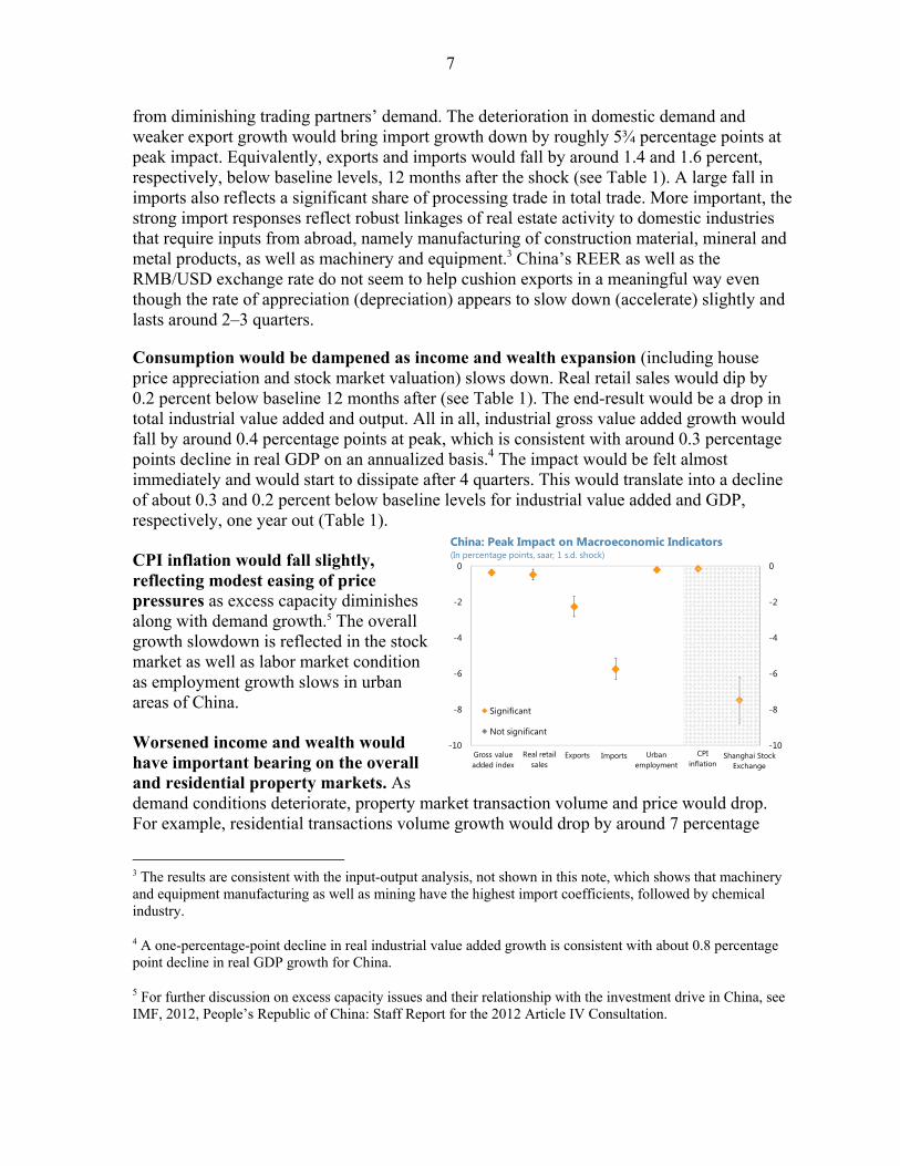
from diminishing trading partners’ demand. The deterioration in domestic demand and weaker export growth would bring import growth down by roughly 5¾ percentage points at peak impact. Equivalently, exports and imports would fall by around 1.4 and 1.6 percent, respectively, below baseline levels, 12 months after the shock (see Table 1). A large fall in imports also reflects a significant share of processing trade in total trade. More important, the strong import responses reflect robust linkages of real estate activity to domestic industries that require inputs from abroad, namely manufacturing of construction material, mineral and metal products, as well as machinery and equipment.3 China’s REER as well as the RMB/USD exchange rate do not seem to help cushion exports in a meaningful way even though the rate of appreciation (depreciation) appears to slow down (accelerate) slightly and lasts around 2–3 quarters.

Consumption would be dampened as income and wealth expansion (including house price appreciation and stock market valuation) slows down. Real retail sales would dip by 0.2 percent below baseline 12 months after (see Table 1). The end-result would be a drop in total industrial value added and output. All in all, industrial gross value added growth would fall by around 0.4 percentage points at peak, which is consistent with around 0.3 percentage points decline in real GDP on an annualized basis.4 The impact would be felt almost immediately and would start to dissipate after 4 quarters. This would translate into a decline of about 0.3 and 0.2 percent below baseline levels for industrial value added and GDP, respectively, one year out (Table 1). CPI inflation would fall slightly, reflecting modest easing of price pressures as excess capacity diminishes along with demand growth.5 The overall growth slowdown is reflected in the stock market as well as labor market condition as employment growth slows in urban areas of China. Worsened income and wealth would have important bearing on the overall and residential property markets. As demand conditions deteriorate, property market transaction volume and price would drop. For example, residential transactions volume growth would drop by around 7 percentage

3 The results are consistent with the input-output analysis, not shown in this note, which shows that machinery and equipment manufacturing as well as mining have the highest import coefficients, followed by chemical industry.

4 A one-percentage-point decline in real industrial value added growth is consistent with about 0.8 percentage point decline in real GDP growth for China.

5 For further discussion on excess capacity issues and their relationship with the investment drive in China, see IMF, 2012, People’s Republic of China: Staff Report for the 2012 Article IV Consultation.

8

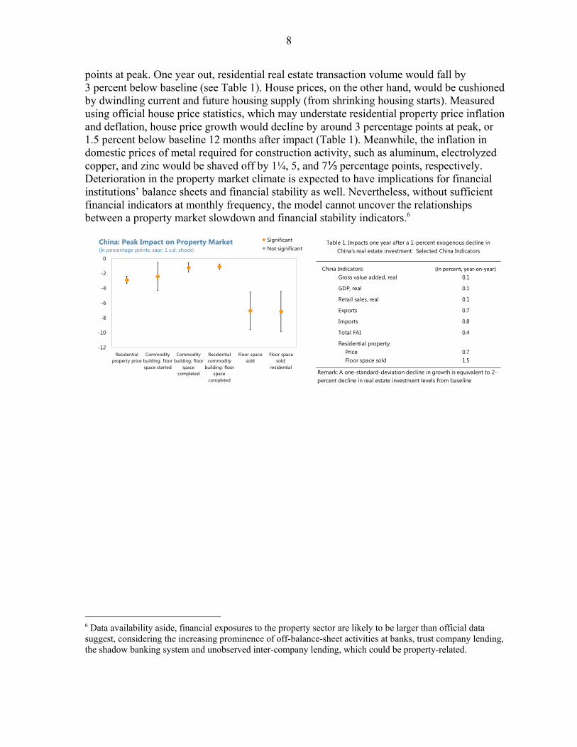
points at peak. One year out, residential real estate transaction volume would fall by 3 percent below baseline (see Table 1). House prices, on the other hand, would be cushioned by dwindling current and future housing supply (from shrinking housing starts). Measured using official house price statistics, which may understate residential property price inflation and deflation, house price growth would decline by around 3 percentage points at peak, or 1.5 percent below baseline 12 months after impact (Table 1). Meanwhile, the inflation in domestic prices of metal required for construction activity, such as aluminum, electrolyzed copper, and zinc would be shaved off by 1¼, 5, and 7⅓ percentage points, respectively. Deterioration in the property market climate is expected to have implications for financial institutions’ balance sheets and financial stability as well. Nevertheless, without sufficient financial indicators at monthly frequency, the model cannot uncover the relationships between a property market slowdown and financial stability indicators.6

6 Data availability aside, financial exposures to the property sector are likely to be larger than official data suggest, considering the increasing prominence of off-balance-sheet activities at banks, trust company lending, the shadow banking system and unobserved inter-company lending, which could be property-related.

-12

-10

-8

-6

-4

-2

0

Residential property price

Commodity building: floor space started

Commodity building: floor

space completed

Residential commodity

building: floor space

completed

Floor space sold

Floor space sold:

residential

SignificantNot significant

China: Peak Impact on Property Market(In percentage points, saar; 1 s.d. shock)

China Indicators: (In percent, year-on-year)

Gross value added, real 0.1

GDP, real 0.1

Retail sales, real 0.1

Exports 0.7

Imports 0.8

Total FAI 0.4

Residential property:Price 0.7Floor space sold 1.5

Table 1. Impacts one year after a 1-percent exogenous decline in China's real estate investment: Selected China Indicators

Remark: A one-standard-deviation decline in growth is equivalent to 2-percent decline in real estate investment levels from baseline

9

-6

-4

-2

0

Aus

tral

ia

Braz

il

Cana

da*

Ger

man

y

Indi

a

Indo

nesi

a

Japa

n

Kore

a UK

US

EU

SignificantNot significant

Peak Impact on Industrial Production(In percentage points, saar; 1 s.d. shock)

* Canada's economic activity is represented by monthly real GDP Index, all industries.

-1

-0.8

-0.6

-0.4

-0.2

0

0.2

Aus

tral

ia

Braz

il

Cana

da*

Ger

man

y

Indi

a

Indo

nesi

a

Japa

n

Kore

a

UK US

EU

Significant

Not significantPeak Impact on Real GDP, implied(In percentage points, saar, 1 s.d. shock)

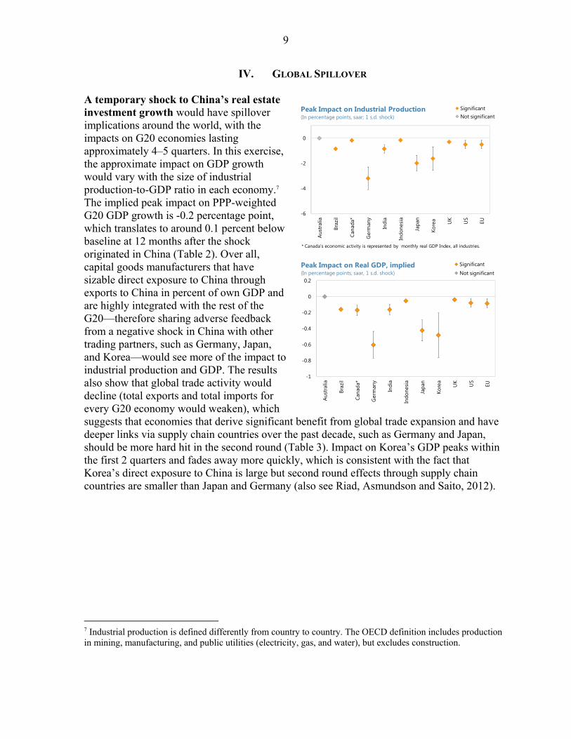
IV. GLOBAL SPILLOVER A temporary shock to China’s real estate investment growth would have spillover implications around the world, with the impacts on G20 economies lasting approximately 4–5 quarters. In this exercise, the approximate impact on GDP growth would vary with the size of industrial production-to-GDP ratio in each economy.7 The implied peak impact on PPP-weighted G20 GDP growth is -0.2 percentage point, which translates to around 0.1 percent below baseline at 12 months after the shock originated in China (Table 2). Over all, capital goods manufacturers that have sizable direct exposure to China through exports to China in percent of own GDP and are highly integrated with the rest of the G20—therefore sharing adverse feedback from a negative shock in China with other trading partners, such as Germany, Japan, and Korea—would see more of the impact to industrial production and GDP. The results also show that global trade activity would decline (total exports and total imports for every G20 economy would weaken), which suggests that economies that derive significant benefit from global trade expansion and have deeper links via supply chain countries over the past decade, such as Germany and Japan, should be more hard hit in the second round (Table 3). Impact on Korea’s GDP peaks within the first 2 quarters and fades away more quickly, which is consistent with the fact that Korea’s direct exposure to China is large but second round effects through supply chain countries are smaller than Japan and Germany (also see Riad, Asmundson and Saito, 2012).

7 Industrial production is defined differently from country to country. The OECD definition includes production in mining, manufacturing, and public utilities (electricity, gas, and water), but excludes construction.

10

-10

-6

-2

2

Aus

tral

ia

Braz

il

Cana

da

Ger

man

y

Indi

a

Japa

n

Kore

a UK

US

EU

SignificantNot significant

Peak Impact on Exports to China(In percentage points, saar; 1 s.d. shock)

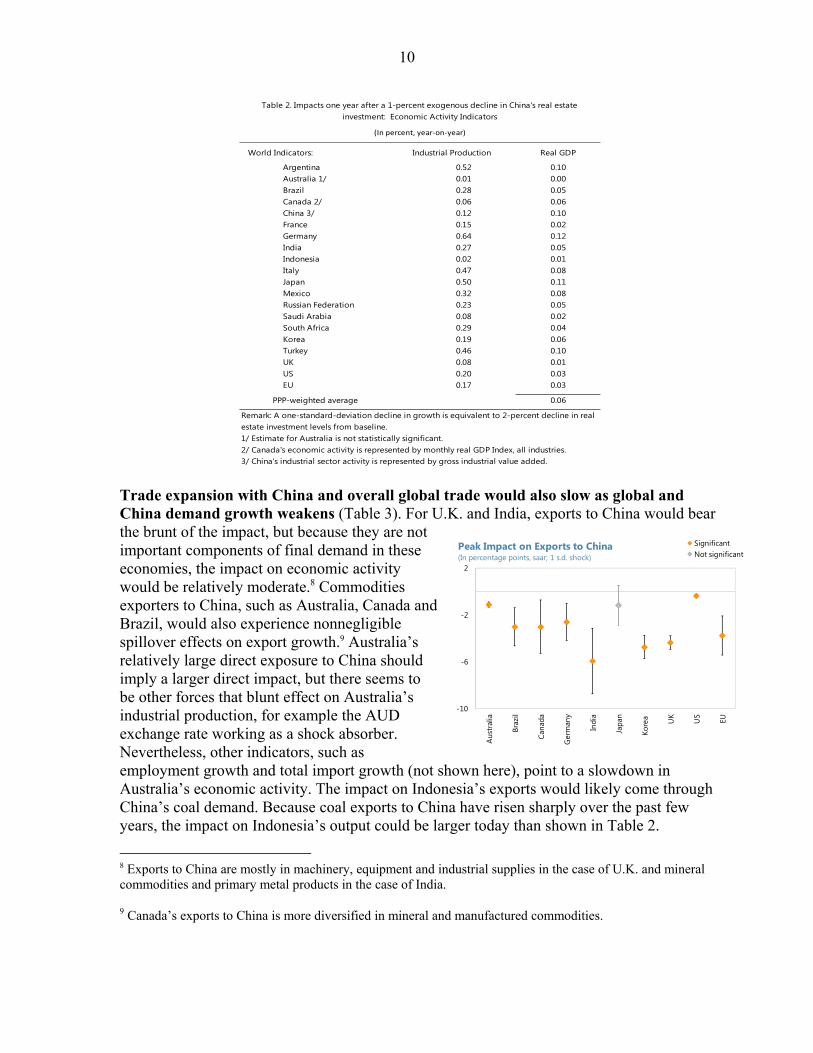
Trade expansion with China and overall global trade would also slow as global and China demand growth weakens (Table 3). For U.K. and India, exports to China would bear the brunt of the impact, but because they are not important components of final demand in these economies, the impact on economic activity would be relatively moderate.8 Commodities exporters to China, such as Australia, Canada and Brazil, would also experience nonnegligible spillover effects on export growth.9 Australia’s relatively large direct exposure to China should imply a larger direct impact, but there seems to be other forces that blunt effect on Australia’s industrial production, for example the AUD exchange rate working as a shock absorber. Nevertheless, other indicators, such as employment growth and total import growth (not shown here), point to a slowdown in Australia’s economic activity. The impact on Indonesia’s exports would likely come through China’s coal demand. Because coal exports to China have risen sharply over the past few years, the impact on Indonesia’s output could be larger today than shown in Table 2.

8 Exports to China are mostly in machinery, equipment and industrial supplies in the case of U.K. and mineral commodities and primary metal products in the case of India.

9 Canada’s exports to China is more diversified in mineral and manufactured commodities.

World Indicators: Industrial Production Real GDP

Argentina 0.52 0.10Australia 1/ 0.01 0.00Brazil 0.28 0.05Canada 2/ 0.06 0.06China 3/ 0.12 0.10France 0.15 0.02Germany 0.64 0.12India 0.27 0.05Indonesia 0.02 0.01Italy 0.47 0.08Japan 0.50 0.11Mexico 0.32 0.08Russian Federation 0.23 0.05Saudi Arabia 0.08 0.02South Africa 0.29 0.04Korea 0.19 0.06Turkey 0.46 0.10UK 0.08 0.01US 0.20 0.03EU 0.17 0.03

PPP-weighted average 0.06

1/ Estimate for Australia is not statistically significant. 2/ Canada's economic activity is represented by monthly real GDP Index, all industries.

3/ China's industrial sector activity is represented by gross industrial value added.

Remark: A one-standard-deviation decline in growth is equivalent to 2-percent decline in real estate investment levels from baseline.

Table 2. Impacts one year after a 1-percent exogenous decline in China's real estate investment: Economic Activity Indicators

(In percent, year-on-year)

11

-6

-4

-2

0

Aus

tral

ia

Braz

il

Cana

da

Ger

man

y

Indi

a

Japa

n

Kore

a UK

US

EU

Significant

Not significantPeak Impact on Stock Market Index(In percentage points, saar; 1 s.d. shock)

-0.7

-0.5

-0.3

-0.1

0.1

0.3

Aus

tral

ia

Cana

da

Ger

nam

y

Indi

a

Italy

Japa

n

Kore

a

UK US

EU

Significant

Not significant

Peak Impact on Sovereign Bond Spreads: 10Y-2Y(In percent; 12-month cumulative; 1 s.d. shock)

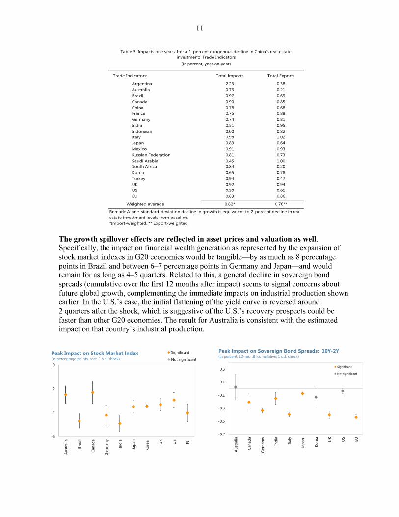
The growth spillover effects are reflected in asset prices and valuation as well. Specifically, the impact on financial wealth generation as represented by the expansion of stock market indexes in G20 economies would be tangible—by as much as 8 percentage points in Brazil and between 6–7 percentage points in Germany and Japan—and would remain for as long as 4–5 quarters. Related to this, a general decline in sovereign bond spreads (cumulative over the first 12 months after impact) seems to signal concerns about future global growth, complementing the immediate impacts on industrial production shown earlier. In the U.S.’s case, the initial flattening of the yield curve is reversed around 2 quarters after the shock, which is suggestive of the U.S.’s recovery prospects could be faster than other G20 economies. The result for Australia is consistent with the estimated impact on that country’s industrial production.

Trade Indicators: Total Imports Total Exports

Argentina 2.23 0.38Australia 0.73 0.21Brazil 0.97 0.69Canada 0.90 0.85China 0.78 0.68France 0.75 0.88Germany 0.74 0.81India 0.51 0.95Indonesia 0.00 0.82Italy 0.98 1.02Japan 0.83 0.64Mexico 0.91 0.93Russian Federation 0.81 0.73Saudi Arabia 0.45 1.00South Africa 0.84 0.20Korea 0.65 0.78Turkey 0.94 0.47UK 0.92 0.94US 0.90 0.61EU 0.83 0.86

Weighted average 0.82* 0.76**

*Import-weighted. ** Export-weighted.

Table 3. Impacts one year after a 1-percent exogenous decline in China's real estate investment: Trade Indicators

(In percent, year-on-year)

Remark: A one-standard-deviation decline in growth is equivalent to 2-percent decline in real estate investment levels from baseline.

12

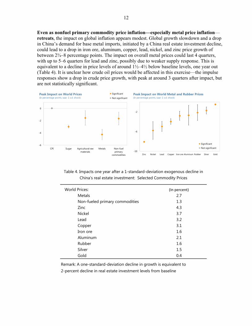
Even as nonfuel primary commodity price inflation—especially metal price inflation—retreats, the impact on global inflation appears modest. Global growth slowdown and a drop in China’s demand for base metal imports, initiated by a China real estate investment decline, could lead to a drop in iron ore, aluminum, copper, lead, nickel, and zinc price growth of between 2¾–8 percentage points. The impact on overall metal prices could last 4 quarters, with up to 5–6 quarters for lead and zinc, possibly due to weaker supply response. This is equivalent to a decline in price levels of around 1½–4½ below baseline levels, one year out (Table 4). It is unclear how crude oil prices would be affected in this exercise—the impulse responses show a drop in crude price growth, with peak at around 3 quarters after impact, but are not statistically significant.

-6

-4

-2

0

CPI Sugar Agricultural raw materials

Metals Non-fuel primary

commodities

Significant

Not significantPeak Impact on World Prices(In percentage points, saar; 1 s.d. shock)

-10

-6

-2

Zinc Nickel Lead Copper Iron ore Aluminum Rubber Silver Gold

Significant

Not significant

Peak Impact on World Metal and Rubber Prices(In percentage points, saar; 1 s.d. shock)

World Prices: (In percent)

Metals 2.7Non-fueled primary commodities 1.3Zinc 4.3Nickel 3.7Lead 3.2Copper 3.1Iron ore 1.6Aluminum 2.1Rubber 1.6Silver 1.5Gold 0.4

Table 4. Impacts one year after a 1-standard-deviation exogenous decline in China's real estate investment: Selected Commodity Prices

Remark: A one-standard-deviation decline in growth is equivalent to 2-percent decline in real estate investment levels from baseline

13

V. CONCLUSION Real estate investment account for a quarter of total fixed asset investment in China. The impact on economic activity of a hypothetical collapse in real estate investment in China is sizable, with large spillovers to a number of China’s trading partners. A 1-percent decline in China’s real estate investment would shave about 0.1 percent off China’s real GDP within the first year, with negative spillover impacts to China’s G20 trading partners that would cause global output to decline by roughly 0.06 percent from baseline. Japan, Korea, and Germany would be among the hardest hit. In that event, commodity prices, especially metal prices, could fall by as much as 0.8–2.2 percent below baseline one year after the shock.

Overall, capital goods manufacturers that have sizable direct exposure to China—especially Japan and Korea—and are highly integrated with the rest of the G20—therefore sharing adverse feedback from a negative shock in China with other trading partners—such as Germany and Japan—would experience larger decline in industrial production and GDP. Worsened global growth prospects would be reflected in asset prices and sovereign bond spreads. In that event, commodity prices, especially construction-related metal prices, would also fall.

Our sample contains at least one full cycle of real estate investment and property market in China, and represents China’s increasing integration with the world economy. Strictly from a statistical point of view, we expect a priority that this relatively short sample will make statistical relationships harder to detect and will be an important constraint on the richness of the models. Nevertheless, as the results suggest, there is still sufficient statistical information in the sample that allows us to learn something useful about China’s interaction with the world in the recent past. It is important to stress, however, that China is more important to the global economy today than our sample would suggest and a China investment bust is not likely to be a linear event as measured by the model. The impact on G20 trading partners and therefore global growth today should be larger than we report.

14

References Bernanke, B., J. Boivin, and P. Eliasz, 2005, “Measuring the Effects of Monetary Policy: A

Factor-Augmented Vector Autoregressive (FAVAR) Approach,” Quarterly Journal Of Economics, Vol. 120, No.1, pp. 387–422.

Boivin, J. and M. Giannoni, 2008, “Global Forces and Monetary Policy Effectiveness,”

NBER Working Paper 13736. Interational Monetary Fund, 2012, “People’s Republic of China: Staff Report for the 2012

Article IV Consultation,” IMF Country Report No. 12/195. Riad, N., I. Asmundson and M. Saito, 2012, “China's Trade Balance Adjustment: Spillover

Effects,” 2012 Spillover Report–Background Papers (Washington: International Monetary Fund).

Stock, J. and M. Watson (2002), “Macroeconomic Forecasting Using Diffusion Indexes,”

Journal of Business Economics and Statistics, XX: II pp 147–62.

15

Appendix A: The China–G20 Macro Financial FAVAR

Why a FAVAR? The factor-augmented vector autoregressive (FAVAR) approach offers a simple and agnostic tool to identify and measure the spillover effects of innovations in investment and real estate investment in China on various international macroeconomic, financial, trade, expectations and labor market variables. At the philosophical level, the approach works on a plausible assumption that policy makers and market participants face information constraints (similar to the econometrician) when they try to gauge economic conditions and developments, e.g. economic activity, price pressures, liquidity, and credit conditions, etc. They try to overcome these constrains by exploiting the information from a very large set of economic indicators

Technically, the approach offers a natural solution to the degrees-of-freedom problem in standard VARs by effectively conditioning VAR analysis of shocks on a large number of time series while exploiting the statistical advantages of restricting the analysis to a small number of estimated factors, which usefully summarize those time series. As it requires only a plausible identification of the shocks and not a precise identification (restriction) of the remainder of the macroeconomic model, simplicity of the VAR’s approach is retained.

By conditioning the analysis on a rich information set, the approach addresses three well-known criticisms of the low-dimensional VARs, structural VARs, and Bayesian VARs in several applications. First, it resolves the problem of mis-measurement of shocks or policy innovations—typically arising from the inability to control for information market participants or policy makers use—which leads to incorrect estimated responses of economic variables to those innovations.10 Second, it does not require the analysis to rest only on specific observable measures to represent certain economic concepts. For example, the concept of “economic activity” cannot be perfectly captured by one indicator, such as real GDP or industrial production. Including multiple indicators, e.g. retail sales and employment, could represent the concept better. “Price pressures” may be better represented by various measures of prices—CPI, PPI, commodity (metal, nonmetal, fuel or nonfuel) prices. “Interest rates” and “liquidity and credit conditions” cannot easily be represented by one or two series, but are reflected in a wider range of economic indicators.11

Finally, for the purposes of policy analysis and model validation, the impulse responses can be observed for a large set of variables that policy makers and markets care about.

10 The “price puzzle”, which occurs in monetary VARs because the models do not capture the signals about future inflation central banks may have, is an oft-cited example, and is usually resolved in a clumsy, ad hoc manner in standard VARs.

11 If a true system is a FAVAR, but is estimated as a standard VAR (with factors omitted), the estimated VAR coefficients and the impulse response coefficients will be biased.

16

The Model Briefly, the model is a stable FAVAR in growth (except for balances and interest rates) with five common factors for each region (China and the rest of the G20 economies) and China’s real estate investment. The model uses one lag. The Cholesky factor from the residual covariance matrix is used to orthogonalize the impulses, which imposes an ordering of the variables in the VAR and treats real estate investment as exogenous in the period of shock. Specifically, the VAR ordering restricts China’s real estate investment to exogenously impact China’s common factors which then spillover onto global factors in the immediate period (one month) after the shock in a recursive fashion. By construction, there is no need to identify the factors separately because each region-specific set of common factors (or principal components) is an independent linear combination that spans the respective data set. The results are therefore robust to re-ordering within factor groups.

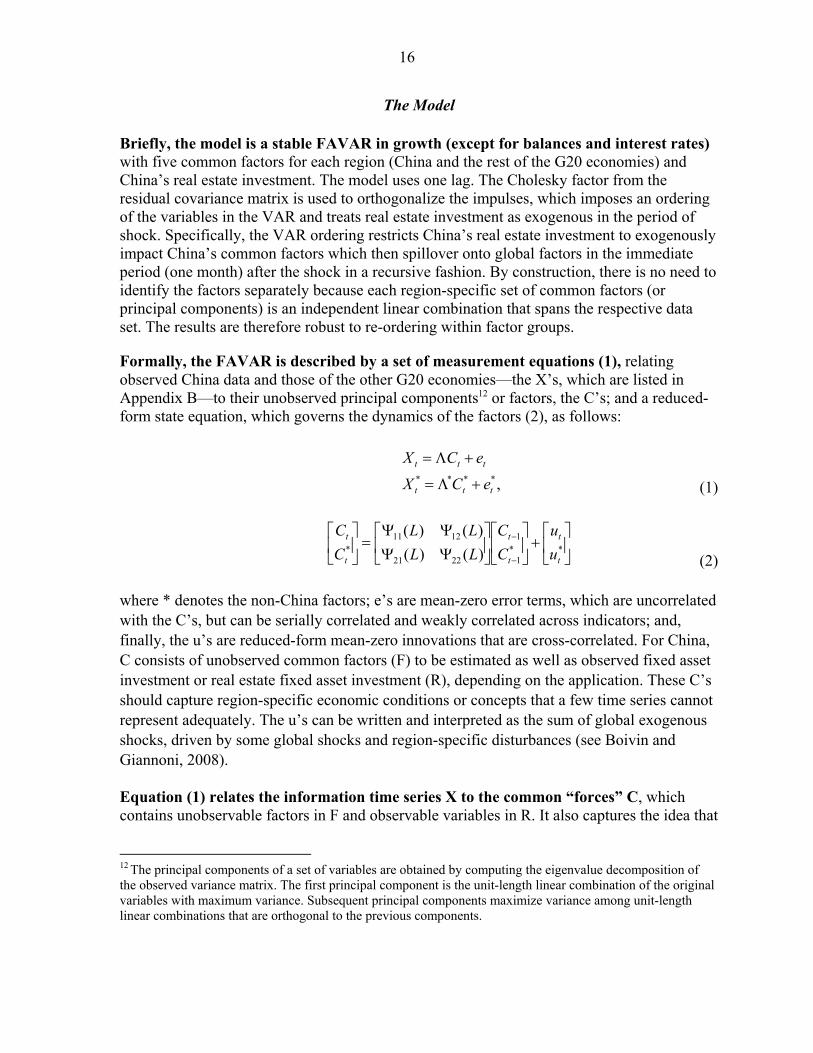
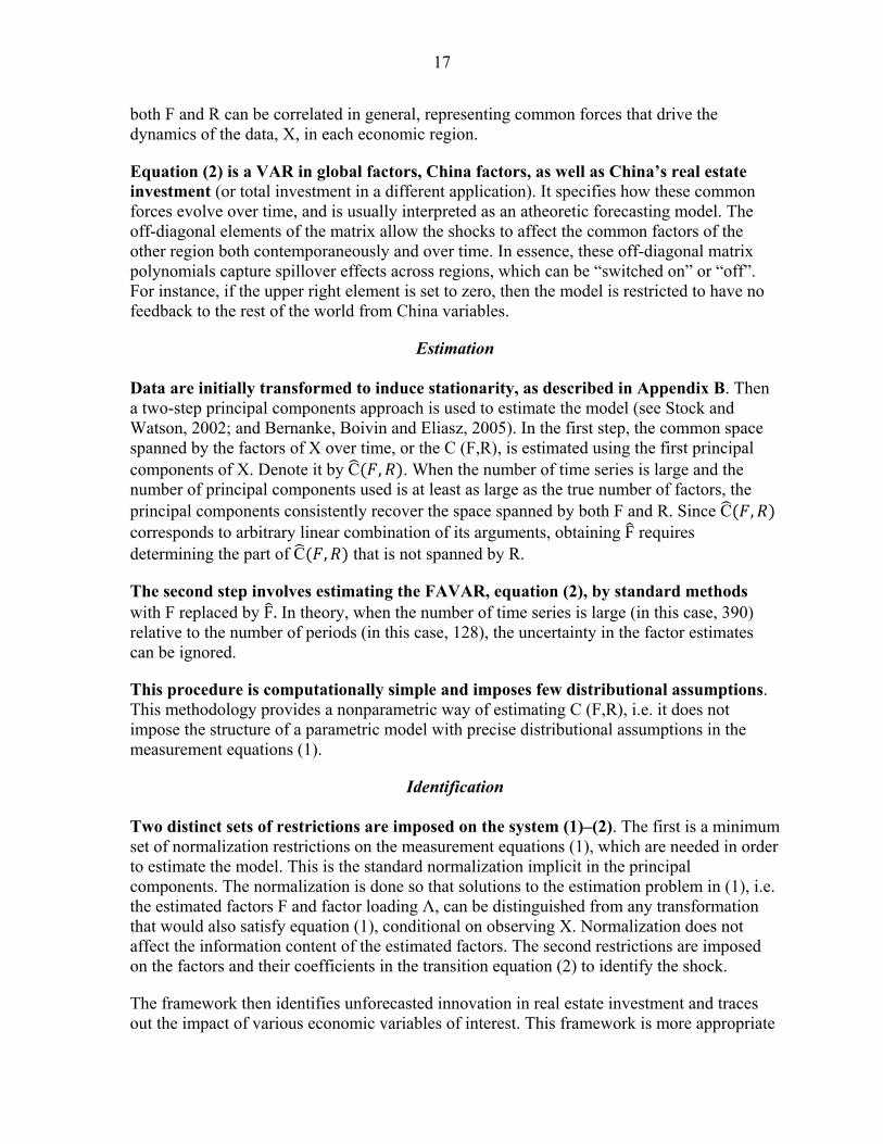
Formally, the FAVAR is described by a set of measurement equations (1), relating observed China data and those of the other G20 economies—the X’s, which are listed in Appendix B—to their unobserved principal components12 or factors, the C’s; and a reduced-form state equation, which governs the dynamics of the factors (2), as follows:

(1)

(2) where * denotes the non-China factors; e’s are mean-zero error terms, which are uncorrelated with the C’s, but can be serially correlated and weakly correlated across indicators; and, finally, the u’s are reduced-form mean-zero innovations that are cross-correlated. For China, C consists of unobserved common factors (F) to be estimated as well as observed fixed asset investment or real estate fixed asset investment (R), depending on the application. These C’s should capture region-specific economic conditions or concepts that a few time series cannot represent adequately. The u’s can be written and interpreted as the sum of global exogenous shocks, driven by some global shocks and region-specific disturbances (see Boivin and Giannoni, 2008). Equation (1) relates the information time series X to the common “forces” C, which contains unobservable factors in F and observable variables in R. It also captures the idea that

12 The principal components of a set of variables are obtained by computing the eigenvalue decomposition of the observed variance matrix. The first principal component is the unit-length linear combination of the original variables with maximum variance. Subsequent principal components maximize variance among unit-length linear combinations that are orthogonal to the previous components.

,****ttt

ttt

eCX

eCX

**

1

1

2221

1211* )()(

)()(

t

t

t

t

t

t

u

u

C

C

LL

LL

C

C

17

both F and R can be correlated in general, representing common forces that drive the dynamics of the data, X, in each economic region.

Equation (2) is a VAR in global factors, China factors, as well as China’s real estate investment (or total investment in a different application). It specifies how these common forces evolve over time, and is usually interpreted as an atheoretic forecasting model. The off-diagonal elements of the matrix allow the shocks to affect the common factors of the other region both contemporaneously and over time. In essence, these off-diagonal matrix polynomials capture spillover effects across regions, which can be “switched on” or “off”. For instance, if the upper right element is set to zero, then the model is restricted to have no feedback to the rest of the world from China variables.

Estimation Data are initially transformed to induce stationarity, as described in Appendix B. Then a two-step principal components approach is used to estimate the model (see Stock and Watson, 2002; and Bernanke, Boivin and Eliasz, 2005). In the first step, the common space spanned by the factors of X over time, or the C (F,R), is estimated using the first principal components of X. Denote it by C , . When the number of time series is large and the number of principal components used is at least as large as the true number of factors, the principal components consistently recover the space spanned by both F and R. Since C , corresponds to arbitrary linear combination of its arguments, obtaining F requires determining the part of C , that is not spanned by R.

The second step involves estimating the FAVAR, equation (2), by standard methods with F replaced by F. In theory, when the number of time series is large (in this case, 390) relative to the number of periods (in this case, 128), the uncertainty in the factor estimates can be ignored.

This procedure is computationally simple and imposes few distributional assumptions. This methodology provides a nonparametric way of estimating C (F,R), i.e. it does not impose the structure of a parametric model with precise distributional assumptions in the measurement equations (1).

Identification Two distinct sets of restrictions are imposed on the system (1)–(2). The first is a minimum set of normalization restrictions on the measurement equations (1), which are needed in order to estimate the model. This is the standard normalization implicit in the principal components. The normalization is done so that solutions to the estimation problem in (1), i.e. the estimated factors F and factor loading Λ, can be distinguished from any transformation that would also satisfy equation (1), conditional on observing X. Normalization does not affect the information content of the estimated factors. The second restrictions are imposed on the factors and their coefficients in the transition equation (2) to identify the shock.

The framework then identifies unforecasted innovation in real estate investment and traces out the impact of various economic variables of interest. This framework is more appropriate

18

for our analytical purpose than for monetary policy analysis, as the unforecasted portion of policy interest rate innovations are not interesting in the real world where central banks follow well known monetary policy rules and communicate their actions actively to influence markets.

The second set of restriction is the identification of the structural shocks in the transition equation (2). A recursive structure is assumed where all the factors entering (2) respond with a lag to change in the exogenous variable (real estate investment), ordered last. In this case, there is no need to identify the factors individually, but only the space spanned by the latent factors, F and C*. The Cholesky factor from the residual covariance matrix is used to orthogonalize the impulses, which imposes an ordering of the variables in the VAR and treats real estate investment as exogenous in the period of shock. The results are robust to re-ordering within factor groups.

As a result, no further restrictions are required in (1) and the identification of the shock can be achieved in (2) as if it were a standard VAR.

19

Appendix B: Data Transformation and Sources

Series Country Descriptor SourceDLOG of seasoanally

adjusted seriesDLOG (series already seasonally adjusted by

source)

Seasonal adjustment of

level series

No transformation

Industrial Production Indexs001 Argentina AR: Industrial Monthly Estimates (Index 2000=100 ) CEIC

s002 Australia Australia: Industrial Production (Index 2000=100 ) Haver

s003 Brazil BR: Industrial Production Index (Index 2000=100 ) CEIC

s004 Canada Canada: GDP: All Industries ( Index of : SAAR, Mil.Chn.2002.C$) Haver

s005 France FR: Industrial Production Index (Index 2000=100 SA) CEIC

s006 Germany DE: IPI: Manufacturing (Index 2000=100 ) CEIC

s007 India IN: Industrial Production Index (IPI) (Index 2000=100 ) CEIC

s008 Indonesia ID: Industrial Production Index (IPI) (Index 2000=100 ) CEIC

s009 Italy IT: Industrial Production Index (IPI) (Index 2000=100 ) CEIC

s010 Japan JP: Industrial Production Index (IPI): Mining and Manufacturing (Index 2000=100 ) CEIC

s011 Korea KR: Industrial Production Index (IPI) (Index 2000=100 ) CEIC

s012 Mexico MX: Industrial Production Index (Index 2000=100 ) CEIC

s013 Russia Russia: Output: Industrial Production Index: Total (NSA) (Index 2000=100 ) Haver

s014 Saudi Arabia Saudi Arabia: Crude Petroleum Production (Index 2000=100 ) IFS

s015 South Africa ZA: Manufacturing Production Index (Index 2000=100 ) CEIC

s016 Turkey TR: Industrial Production Index (IPI): NACE 2 (Index 2000=100 ) CEIC

s017 UK UK: Industrial Production Index: Seasonally Adjusted (Index 2000=100 SA) CEIC

s018 US US: Industrial Production Index (Index 2000=100 ) CEIC

s019 EU EU: Industrial Production Index (IPI): EU 27: excl Construction (Index 2000=100 SA) CEIC

Total Exportss020 Argentina Argentina: Exports to World (USD mn) DOTS

s021 Australia Australia: Exports to World (USD mn) DOTS

s022 Brazil Brazil: Exports to World (USD mn) DOTS

s023 Canada Canada: Exports to World (USD mn) DOTS

s024 France France: Exports to World (USD mn) DOTS

s025 Germany Germany: Exports to World (USD mn) DOTS

s026 India India: Exports to World (USD mn) DOTS

s027 Indonesia Indonesia: Exports to World (USD mn) DOTS

s028 Italy Italy: Exports to World (USD mn) DOTS

s029 Japan Japan: Exports to World (USD mn) DOTS

s030 Korea Korea, Republic of: Exports to World (USD mn) DOTS

s031 Mexico Mexico: Exports to World (USD mn) DOTS

s032 Russia Russian Federation: Exports to World (USD mn) DOTS

s033 Saudi Arabia Saudi Arabia: Exports to World (USD mn) DOTS

s034 South Africa South Africa: Exports to World (USD mn) DOTS

s035 Turkey Turkey: Exports to World (USD mn) DOTS

s036 UK United Kingdom: Exports to World (USD mn) DOTS

s037 US United States: Exports to World (USD mn) DOTS

s038 EU European Union (agg): Exports to World (USD mn) DOTS

Total Importss039 Argentina Argentina: Imports from World (USD mn) DOTS

s040 Australia Australia: Imports from World (USD mn) DOTS

s041 Brazil Brazil: Imports from World (USD mn) DOTS

s042 Canada Canada: Imports from World (USD mn) DOTS

s043 France France: Imports from World (USD mn) DOTS

s044 Germany Germany: Imports from World (USD mn) DOTS

s045 India India: Imports from World (USD mn) DOTS

s046 Indonesia Indonesia: Imports from World (USD mn) DOTS

s047 Italy Italy: Imports from World (USD mn) DOTS

s048 Japan Japan: Imports from World (USD mn) DOTS

s049 Korea Korea, Republic of: Imports from World (USD mn) DOTS

s050 Mexico Mexico: Imports from World (USD mn) DOTS

s051 Russia Russian Federation: Imports from World (USD mn) DOTS

s052 Saudi Arabia Saudi Arabia: Imports from World (USD mn) DOTS

s053 South Africa South Africa: Imports from World (USD mn) DOTS

s054 Turkey Turkey: Imports from World (USD mn) DOTS

s055 UK United Kingdom: Imports from World (USD mn) DOTS

s056 US United States: Imports from World (USD mn) DOTS

s057 EU European Union (agg): Imports from World (USD mn) DOTS

Goods Trade Balances058 Argentina Argentina: Trade Balance (USD mn) DOTS

s059 Australia Australia: Trade Balance (USD mn) DOTS

s060 Brazil Brazil: Trade Balance (USD mn) DOTS

s061 Canada Canada: Trade Balance (USD mn) DOTS

s062 France France: Trade Balance (USD mn) DOTS

s063 Germany Gernamy: Trade Balance (USD mn) DOTS

s064 India India: Trade Balance (USD mn) DOTS

s065 Indonesia Indonesia: Trade Balance (USD mn) DOTS

s066 Italy Italy: Trade Balance (USD mn) DOTS

s067 Japan Japan : Trade Balance (USD Mn) DOTS

s068 Korea Korea: Trade Balance (USD mn) DOTS

s069 Mexico Mexico: Trade Balance (USD mn) DOTS

s070 Russia Russia: Trade Balance (USD mn) DOTS

s071 Saudi Arabia Saudi Arabia: Trade Balance (USD mn) DOTS

s072 South Africa South Africa: Trade Balance (USD mn) DOTS

s073 Turkey Turkey: Trade Balance (USD mn) DOTS

s074 UK UK: Trade Balance (USD mn) DOTS

s075 US US: Trade Balance (USD mn) DOTS

s076 EU EU: Trade Balance (USD mn) DOTS

Transformations

Appendix A. Data Sources and Transformations

20

Series Country Descriptor SourceDLOG of seasoanally

adjusted seriesDLOG (series already seasonally adjusted by

source)

Seasonal adjustment of

level series

No transformation

Exports to Chinas077 Argentina Argentina: Exports to China,P.R.: Mainland (USD mn) DOTS

s078 Australia Australia: Exports to China,P.R.: Mainland (USD mn) DOTS

s079 Brazil Brazil: Exports to China,P.R.: Mainland (USD mn) DOTS

s080 Canada Canada: Exports to China,P.R.: Mainland (USD mn) DOTS

s081 France France: Exports to China,P.R.: Mainland (USD mn) DOTS

s082 Germany Germany: Exports to China,P.R.: Mainland (USD mn) DOTS

s083 India India: Exports to China,P.R.: Mainland (USD mn) DOTS

s084 Indonesia Indonesia: Exports to China,P.R.: Mainland (USD mn) DOTS

s085 Italy Italy: Exports to China,P.R.: Mainland (USD mn) DOTS

s086 Japan Japan: Exports to China,P.R.: Mainland (USD mn) DOTS

s087 Korea Korea, Republic of: Exports to China,P.R.: Mainland (USD mn) DOTS

s088 Mexico Mexico: Exports to China,P.R.: Mainland (USD mn) DOTS

s089 Russia Russian Federation: Exports to China,P.R.: Mainland (USD mn) DOTS

s090 Saudi Arabia Saudi Arabia: Exports to China,P.R.: Mainland (USD mn) DOTS

s091 South Africa South Africa: Exports to China,P.R.: Mainland (USD mn) DOTS

s092 Turkey Turkey: Exports to China,P.R.: Mainland (USD mn) DOTS

s093 UK United Kingdom: Exports to China,P.R.: Mainland (USD mn) DOTS

s094 US United States: Exports to China,P.R.: Mainland (USD mn) DOTS

s095 EU European Union (agg): Exports to China,P.R.: Mainland (USD mn) DOTS

Imports from Chinas096 Argentina Argentina: Imports from China,P.R.: Mainland (USD mn) DOTS

s097 Australia Australia: Imports from China,P.R.: Mainland (USD mn) DOTS

s098 Brazil Brazil: Imports from China,P.R.: Mainland (USD mn) DOTS

s099 Canada Canada: Imports from China,P.R.: Mainland (USD mn) DOTS

s100 France France: Imports from China,P.R.: Mainland (USD mn) DOTS

s101 Germany Germany: Imports from China,P.R.: Mainland (USD mn) DOTS

s102 India India: Imports from China,P.R.: Mainland (USD mn) DOTS

s103 Indonesia Indonesia: Imports from China,P.R.: Mainland (USD mn) DOTS

s104 Italy Italy: Imports from China,P.R.: Mainland (USD mn) DOTS

s105 Japan Japan: Imports from China,P.R.: Mainland (USD mn) DOTS

s106 Korea Korea, Republic of: Imports from China,P.R.: Mainland (USD mn) DOTS

s107 Mexico Mexico: Imports from China,P.R.: Mainland (USD mn) DOTS

s108 Russia Russian Federation: Imports from China,P.R.: Mainland (USD mn) DOTS

s109 Saudi Arabia Saudi Arabia: Imports from China,P.R.: Mainland (USD mn) DOTS

s110 South Africa South Africa: Imports from China,P.R.: Mainland (USD mn) DOTS

s111 Turkey Turkey: Imports from China,P.R.: Mainland (USD mn) DOTS

s112 UK United Kingdom: Imports from China,P.R.: Mainland (USD mn) DOTS

s113 US United States: Imports from China,P.R.: Mainland (USD mn) DOTS

s114 EU European Union (agg): Imports from China,P.R.: Mainland (USD mn) DOTS

Terms of Trades115 Argentina Argentina: Terms of Trade (yoy % growth) Haver

s116 Australia Australia: Terms of Trade: Goods: BoP (SA, yoy % growth) Haver

s117 Brazil Brazil: Terms of Trade (yoy % growth) CEIC

s120 Germany Gernamy: Terms of Trade (yoy % growth) CEIC

s123 Italy Italy: Terms of Trade (yoy % growth) CEIC

s124 Japan Japan : Terms of Trade: All Commodities (yoy % growth) Haver

s125 Korea Korea: Terms of Trade (yoy % growth) CEIC

s126 Mexico Mexico: Terms of Trade (yoy % growth) Haver

s127 Russia Russia: Terms of Trade (yoy % growth) Haver

s129 South Africa South Africa: Terms of Trade: sa: Excluding Gold (yoy % growth) Haver

s130 Turkey Turkey: Terms of Trade (yoy % growth) Haver

s131 UK UK: Terms of Trade (yoy % growth) CEIC

s132 US US: Terms of Trade: All Imports and exports (yoy % growth) Haver

s133 EU EU: Terms of Trade EU 27: ACP (yoy % growth) Haver

Short-Term Interest Ratess134 Argentina Argentina: Interest Rates: Savings Deposits 30-59 Days (% per annum) Haver

s135 Australia Australia: BBA: 3-Month London Interbank Offered Rate: Based on A$ (%, AVG) Haver

s136 Brazil Brazil: Short-term interest rate Haver

s137 Canada Canada: Treasury Bills: 3-Months (AVG, %) Haver

s138 France France: Treasury Bills, Bid Rate: 3-Month (AVG, %) Haver

s139 Germany Germany: 3-Month Interbank Offered Rate {FIBOR} (%) Haver

s140 India IN: Treasury Bills: Cut Off Yield: Auction: 3 Months (% pa) CEIC

s142 Italy Italy: Interbank Rate: 3-Month (EOP, %) Haver

s143 Japan JP: Financing Bills: Rate: 3 Months (% pa) Haver

s145 Mexico Mexico: 91-Day Treasury Certificates (%) Haver

s148 South Africa South Africa: Treasury Bill Tender Rate, 91-Days (Avg, %) CEIC

s149 Turkey Turkey: Interest Rates: 3 Month Time Deposits (% p.a.) Haver

s150 UK UK: Sterling Interbank Lending Rate, 3-months(AVG, %) Haver

s151 US US: Short Term Interest Rate: Month End: Treasury Bills: 3 Months (% pa) Haver

s152 EU Euro Area 11-17: 3-Month Deposits (%) CEIC

Bond Spreadss154 Australia Australia: Bond Spread: Treasury Bonds: 10 - 2 Years (AVG, % p.a.) Haver

s156 Canada Canada: Bond Spread: (10-Year & Over -- 1 to 3 year) Bond Yield Average ( %) Haver

s158 Germany Germany: Bond Spread: Gov Bond Yields: Ave Resid Maturity: (9 to 10 -- 2 to 3 Years) (%) Haver

s159 India IN: Bond Spread: Government Securities Yield: (10 -- 2) Years (% pa) CEIC

s161 Italy IT: Bond Spread: Government Treasury Bonds Yield: 10 -- 3 Year (% pa) CEIC

s162 Japan Japan: Bond Spread: Benchmark Government Bond Yield: 10 -- 2 Year (AVG, % p.a.) Haver

s163 Korea KR: Bond Spread: Bond Yield: Month Avg: Treasury Bond: 10 -- 1 Yr Maturity (% pa) CEIC

s167 South Africa ZA: Bond Spread: Government Bonds Yield: Monthly Avg: 10 -- 0 to 3 Years (% p.a.) CEIC

s169 UK UK: Generic Bond Spread: 10Y -- 2Y Bloomberg

s170 US US: Bond Spread: 10 -- 2-Year Treasury Note Yield at Constant Maturity (% p.a.) CEIC

s171 EU EU: Generic Bond Spread: 10Y -- 2Y Bloomberg

Transformations

21

Series Country Descriptor SourceDLOG of seasoanally

adjusted seriesDLOG (series already seasonally adjusted by

source)

Seasonal adjustment of

level series

No transformation

Exchange Rates172 Argentina Argentina: Exchange Rate (NC/USD) INS

s173 Australia Australia: Exchange Rate (NC/USD) INS

s174 Brazil Brazil: Exchange Rate (NC/USD) INS

s175 Canada Canada: Exchange Rate (NC/USD) INS

s176 France France: Exchange Rate (NC/USD) INS

s177 Germany Germany: Exchange Rate (NC/USD) INS

s178 India India: Exchange Rate (NC/USD) INS

s179 Indonesia Indonesia: Exchange Rate (NC/USD) INS

s180 Italy Italy: Exchange Rate (NC/USD) INS

s181 Japan Japan: Exchange Rate (NC/USD) INS

s182 Korea Korea, Republic of: Exchange Rate (NC/USD) INS

s183 Mexico Mexico: Exchange Rate (NC/USD) INS

s184 Russia Russian Federation: Exchange Rate (NC/USD) INS

s185 Saudi Arabia Saudi Arabia: Exchange Rate (NC/USD) INS

s186 South Africa South Africa: Exchange Rate (NC/USD) INS

s187 Turkey Turkey: Exchange Rate (NC/USD) INS

s188 UK United Kingdom: Exchange Rate (NC/USD) INS

s190 EU Euro Area: Exchange Rate (NC/USD) INS

Loans and Credits192 Australia Australia: Credit including Securitized Housing Loans (billion NC) Haver

s193 Brazil BR: Loans: Financial System (billion NC) CEIC

s194 Canada Canada: Business & Household Credit (billion NC) Haver

s195 France France: Total Outstanding Loans by Monetary & Finan Inst (billion NC) Haver

s196 Germany DE: Loans: MFIs: Domestic Enterprises & Household (billion NC) Haver

s197 India IN: CS: Domestic Credit (billion NC) CEIC

s200 Japan JP: Loans & Discounts: FI: Total (billion NC) CEIC

s201 Korea KR: Loans of Commercial and Specialized Banks (CSB): Total (billion NC) CEIC

s202 Mexico MX: Commercial Banks: Outstanding Loan: Private Sector (billion NC) CEIC

s203 Russia Russia: Loans in Rubles and FC (billion NC) Haver

s205 South Africa ZA: Banks: Assets: Deposits, Loans & Advances (billion NC) CEIC

s206 Turkey TR: Domestic Loans (billion NC) CEIC

s207 UK UK: Bank Lending: GBP and Foreign Currency (billion NC) Haver

s208 US US: Bank Credit: All Commercial Banks (billion NC, SA) Haver

s209 EU EU: MFIs Loans: Outstanding: Non Financial Sector (billion NC) CEIC

CPIs210 Argentina AR: Consumer Price Index (2010 = 100 ) CEIC

s211 Australia Australia: CPI {Market Prices}: Total excl Volatile Items (NSA) (2010 = 100 ) Haver

s212 Brazil BR: INPC: General (2010 = 100 ) CEIC

s213 Canada Canada: CPI: All Items (SA) (2010 = 100 SA) Haver

s214 France FR: Consumer Price Index (CPI) (2010 = 100 ) CEIC

s215 Germany DE: Consumer Price Index (CPI): Overall (2010 = 100 ) CEIC

s218 Italy IT: Consumer Price Index: (2010 = 100 ) CEIC

s219 Japan JP: Consumer Price Index (2010 = 100 ) CEIC

s220 Korea KR: Consumer Price Index (2010 = 100 ) CEIC

s221 Mexico MX: Consumer Price Index (2010 = 100 ) CEIC

s222 Russia Russia: Consumer Price Index (2010 = 100 ) Haver

s223 Saudi Arabia SA: Cost of Living Index (2010 = 100 ) CEIC

s226 UK UK: UK: Harmonized Index of Consumer Price (HICP) (2010 = 100 ) CEIC

s227 US US: Consumer Price Index: Urban (2010 = 100 ) CEIC

s228 EU EU: Consumer Price Index: sa (2010 = 100 SA) CEIC

s229 Argentina AR: Producer Basic Price Index (2010 = 100 ) CEIC

PPIs230 Australia Australia: Price index: Preliminary commodities: Total (2010 = 100) Haver

s231 Brazil BR: Broad Producer Price Index: FGV: IPA-M (2010 = 100) CEIC

s232 Canada Canada: Raw Materials Purchase Price Index (NSA) (2010 = 100) Haver

s234 Germany DE: Producer Price Index (PPI) (2010 = 100) CEIC

s238 Japan JP: Corporate Goods Price Index (CGPI): Domestic: All Commodities (2010 = 100) CEIC

s239 Korea KR: Producer Price Index: All Commodities and Services (2010 = 100) CEIC

s240 Mexico MX: Producer Price Index (2010 = 100) CEIC

s241 Russia Russia: PPI (2010 = 100) GSTS

s243 South Africa ZA: Production Price Index (PPI-00): Domestic Output (DO) (2010 = 100) CEIC

s245 UK UK: PPI: Input: Net Sector: All Products (2010 = 100) CEIC

s246 US US: PPI: Intermediate Materials (IM) (2010 = 100) CEIC

s247 EU EU: PPI: EU 27: Industry: excl Construction (2010 = 100) CEIC

Employments248 Argentina Argentina: Urban Employed (Thousand) Haver

s249 Australia Australia: No of Employed (Thousand) IFS

s251 Canada Canada: Employment: Both Sexes, 15 Years & Over (NSA, Thousand) Haver

s252 France France: Total Employment: Total (SA, Thousand) Haver

s253 Germany DE: Employment: Germany (Person thousand) CEIC

s256 Italy Italy: Total Employment: Total Economy (NSA, Thousand) Haver

s257 Japan JP: Employment: Total (Person thousand) CEIC

s258 Korea KR: Employment (Person thousand) CEIC

s260 Russia Russia: Labor Market: Employment (NSA, Thousand) Haver

s264 UK UK: Employment: sa: Total (Person thousand) CEIC

s265 US US: Employment (Person thousand) CEIC

s266 EU EU: Unemployment: EU 27 (Person thousand) Haver

Transformations

22

Series Country Descriptor SourceDLOG of seasoanally

adjusted seriesDLOG (series already seasonally adjusted by

source)

Seasonal adjustment of

level series

No transformation

Stock Exchange Indexs267 Argentina Argentina: Argentina Merval Index Haver

s268 Australia Australia: All Ordinaries Indx Haver

s269 Brazil Brazil: Brazil Bovespa Index Haver

s270 Canada Canada: S&P/Tsx Composite Index Haver

s271 France France: Cac 40 Index Haver

s272 Germany Gernamy: Dax Index Haver

s273 India India: Bse Sensex 30 Index Haver

s274 Indonesia Indonesia: Jakarta Composite Index Haver

s275 Italy Italy: Dj Italy Stock Index Haver

s276 Japan Japan : Nikkei 225 Haver

s277 Korea Korea: Mexico Ipc Index Haver

s278 Mexico Mexico: Micex Index Haver

s279 Russia Russia: Tadawul All Share Index Haver

s280 Saudi Arabia Saudi Arabia: Ftse/Jse Africa Top40 Ix Haver

s281 South Africa South Africa: Kospi Index Haver

s282 Turkey Turkey: Ise National 100 Index Haver

s283 UK UK: Ftse 100 Index Haver

s284 US US: S&P 500 Index Haver

s285 EU EU: Ftseurofirst 300 Index Haver

Money Supply M2s287 Australia Australia: Broad Money (Millions, National Currency) IFS

s288 Brazil Brazil: Money Supply, M2 (Millions, National Currency) Haver

s289 Canada Canada: M2 {Gross} (Millions, National Currency) Haver

s290 France France: Money Supply: M2 (Millions, National Currency) Haver

s291 Germany Germany: Money Supply: M2 (Millions, National Currency) Haver

s292 India India: Money Supply: M2 (Millions, National Currency) Haver

s293 Indonesia Indonesia: Broad Money: Broad Money [M2] (Millions, National Currency) Haver

s294 Italy Italy: Money Supply, M2 (Millions, National Currency) Haver

s295 Japan Japan : M2 (Period Average) (Millions, National Currency) IFS

s296 Korea Korea: Money Supply: M2 (Millions, National Currency) Haver

s297 Mexico Mexico: M2 (Millions, National Currency) IFS

s298 Russia Russia: Money Supply ["National Definition"]: M2(Millions, National Currency) Haver

s299 Saudi Arabia Saudi Arabia: Money Supply: M2(Millions, National Currency) Haver

s300 South Africa South Africa: Monetary Aggregates: M2 (Millions, National Currency) Haver

s301 Turkey Turkey: Money Supply: M2(Millions, National Currency) Haver

s302 UK UK: Money Supply M2(Millions, National Currency) CEIC

s303 US Money Stock: M2(Millions, National Currency) Haver

s304 EU EA 11-17: ECB Money Supply: M2 (Millions, National Currency) Haver

Goods and Services Balances305 Argentina Argentina: Balance of Payments: Goods & Services Balance Haver

s306 Australia Australia: BOP: Goods and Services Trade Balance Haver

s307 Brazil Brazil: BOP: Current Account: Goods & Services Balance Haver

s308 Canada Canada: Current Account: Goods and Services Balance Haver

s309 France France: BOP: Current Acct: Goods & Services Balance Haver

s310 Germany Germany: BOP: Current Account: Balance of Trade: Goods & Services Haver

s311 India India: BOP: Goods and Services Haver

s312 Indonesia Indonesia: BOP: Trade in Goods & Services: Balance Haver

s313 Italy Italy: BOP: Current Account: Goods & Services Haver

s314 Japan Japan: BOP: Current Account Balance: Goods And Services Haver

s315 Korea Korea: BOP: Trade in Goods & Services: Balance Haver

s316 Mexico Mexico: BOP: Current Acct, Goods & Services Haver

s317 Russia Russia: BOP: Balance on Goods & Services Haver

s319 South Africa South Africa: BOP: Goods & Services Balance Haver

s320 Turkey Turkey: BOP: Balance of Goods & Services Haver

s321 UK U.K.: Current Account: Trade Balance: Goods and Services Haver

s322 US Trade Balance: Goods and Services, BOP Basis Haver

s323 EU EA 17: BOP: Curr Acct: Net: Goods & Services Haver

World Price Indicatorss324 World World: Consumer Prices (2005=100, NSA) IFS

s326 World World: Avg Crude Price of UK Brt Lt/Dubai Med/Alaska NS heavy (US$/Bbl) IFS

s327 World World: Commodity Price: Sugar, Caribbean {NY} (US cts/lb) IFS

s328 World World: Commodity Price: Linseed Oil, Any Origin (US$/MT) IFS

s329 World World: Commodity Price Index: All Commodities (2005=100) IFS

s330 World World: Commodity Price Index: Food (2005=100) IFS

s331 World World: Commodity Price Index: Beverages (2005=100) IFS

s332 World World: Commodity Price Index: Agricultural Raw Materials (2005=100) IFS

s333 World World: Commodity Price Index: Metals (2005=100) IFS

s334 World World: Non-fuel Primary Commodities Index (2005=100) IFS

s335 World World: Commodity Price Index: Linseed Oil {Any Origin} (2005=100) IFS

s336 World World: Spot Price Idx of UK Brt Lt/Dubai Med/Alaska NS heavy (2005=100) IFS

s337 World World: Commodity Price Index: Sugar, Caribbean {NY} (2005=100) IFS

s344 Canada Canada: Aluminum Canada/Uk IFS

s345 Australia Australia: Coal Australia Index IFS

s346 United Kingdom United Kingdom: Copper Uk (London) IFS

s347 United Kingdom United Kingdom: Gold London Av 2Nd Fix IFS

s348 Brazil Brazil: Iron Ore Brazil (N.Sea.Ports) IFS

s349 United Kingdom United Kingdom: Lead U.K.(London) IFS

s350 United States United States: Natural Gas Index - Us IFS

s351 Canada Canada: Nickel Canada Can/Ports IFS

s352 World World: Averge Crude Price: 3 Spot Price Index IFS

s353 United States United States: Texas Spot Price Index IFS

s354 Thailand Thailand: Rice Thailand (Bangkok) IFS

s355 Malaysia Malaysia: Rubber Malaysia(Singapore) IFS

s356 United States United States: Silver U.S.(New York) IFS

s357 United States United States: Soybeans Us(Rotterdam) IFS

s358 United States United States: Soybean Oil Us(Rot'Dam) IFS

s359 United Kingdom United Kingdom: Tin All Origins(London) IFS

s360 United Kingdom United Kingdom: Zinc U.K.(London) IFS

Transformations

23

Series Country Descriptor SourceDLOG of seasoanally

adjusted seriesDLOG (series already seasonally adjusted by

source)

Seasonal adjustment of

level series

No transformation

China Indicatorss361 China China: Index of Gross Value Added in 1990 Prices Haver

s362 China China,P.R.: Mainland: Exports to World (USD mn) DOTS

s363 China China,P.R.: Mainland: Imports from World (USD mn) DOTS

s365 China CN: Nominal Lending Rate: Short Term: 6 Month (% pa) CEIC

s367 China China,P.R.: Mainland: Exchange Rate (NC/USD) INS

s368 China CN: Loan (RMB bn) CEIC

s369 China CN: Consumer Price Index CEIC

s370 China CN: Producer Price Index CEIC

s371 China China: Urban Employment: Total (NSA, Thous) Haver

s372 China China: Index: Shanghai Stock Exchange: Composite CEIC

s373 China China: Money Supply: M2 (SA, Mil.Yuan) Haver

s374 China CHN: BoP: Service & Goods Haver

s375 China CN: Trade Balance (DOTS, USD mn) DOTS

s376 China National Accounts, Private Final Consumption Expenditure, Real CEIC

s377 China National Accounts, Gross Fixed Capital Formation, Private, Real CEIC

s378 China National Accounts, Gross Fixed Capital Formation, Private, Private Corporations, Real CEIC

s379 China National Accounts, GFCF, Private, Households Incl. Private Non-profit Inst., Real CEIC

s380 China CN: REAL Fixed Asset Investment (RMB mn) CEIC

s385 China CN: Exports: Primary Product CEIC

s386 China CN: Exports: Primary Product: Food and Live Animal CEIC

s387 China CN: Exports: Primary Product: Beverage and Tobacco CEIC

s388 China CN: Exports: Primary Product: Crude Material, Inedible , Except Fuel CEIC

s389 China CN: Exports: Primary Product: Mineral Fuel, Lubricant & Related Material CEIC

s390 China CN: Exports: Primary Product: Animal and Vegetable Oil, Fat and Waxes CEIC

s391 China CN: Exports: Manufacture CEIC

s392 China CN: Exports: Manufacture: Chemical and Related Product CEIC

s393 China CN: Exports: Manufacture: Manufactured Goods CEIC

s394 China CN: Exports: Manufacture: Machinery and Transport Equipment CEIC

s395 China CN: Exports: Manufacture: Misc Mfg Article CEIC

s396 China CN: Exports: Manufacture: Unclassified Goods CEIC

s397 China CN: Imports: Primary Product CEIC

s398 China CN: Imports: Primary Product: Food and Live Animal CEIC

s399 China CN: Imports: Primary Product: Beverage and Tobacco CEIC

s400 China CN: Imports: Primary Product: Crude Material, Inedible , Except Fuel CEIC

s401 China CN: Imports: Primary Product: Mineral Fuel, Lubricant & Related Material CEIC

s402 China CN: Imports: Primary Product: Animal and Vegetable Oil, Fat and Waxes CEIC

s403 China CN: Imports: Manufacture CEIC

s404 China CN: Imports: Manufacture: Chemical and Related Product CEIC

s405 China CN: Imports: Manufacture: Manufactured Goods CEIC

s406 China CN: Imports: Manufacture: Machinery and Transport Equipment CEIC

s407 China CN: Imports: Manufacture: Misc Manufactured Article CEIC

s408 China CN: Imports: Manufacture: Unclassified Goods CEIC

s409 China CN: Commodity Bldg Selling Price: Residential (RMB/Sq m) CEIC

s416 China CN: Effective Exchange Rate Index: BIS: Real (2010=100 ) CEIC

s417 China CN: Effective Exchange Rate Index: BIS: Nominal (2010=100 ) CEIC

s419 China CN: Transaction Price: Round Steel: 16mm, HPB235 (RMB/Ton ) CEIC

s420 China CN: Transaction Price: Electrolyse Copper, No 1 (RMB/Ton) CEIC

s421 China CN: Transaction Price: Aluminum: AOO (RMB/Ton) CEIC

s422 China CN: Transaction Price: Zinc, No 1 (RMB/Ton) CEIC

s423 China CN: Import Price: Iron Ore & Concentrate (USD/Ton) CEIC

s425 China CN: Service Price: 36 City Avg: Electricity: for Resident: 220v (RMB/100KWH) CEIC

s426 China CN: Service Price: 36 City Avg: Pipe Gas: for Resident (RMB/Cub m) CEIC

s436 China CN: Import Price: Crude Oil (USD/Ton) CEIC

s437 China CN: Export Price: Crude Oil (USD/Ton) CEIC

s438 China CN: FAI: Primary Industry (RMB mn) CEIC

s439 China CN: FAI: Secondary Industry (SI) (RMB mn) CEIC

s443 China CN: FAI: SI: Construction (RMB mn) CEIC

s444 China CN: FAI: Tertiary Industry (RMB mn) CEIC

s464 China CN: Floor Space Started: Commodity Bldg (CB) (Sq meter th) CEIC

s468 China CN: Floor Space Completed: Commodity Bldg (CB) (Sq meter th) CEIC

s469 China CN: Floor Space Completed: CB: Residential (Sq meter th) CEIC

s472 China CN: Floor Space Sold: (Sq meter th) CEIC

s473 China CN: Floor Space Sold: Residential (Sq m th) CEIC

s481 China CN: Land Area Purchased: (Sq meter th) CEIC

s483 China CN: Real Estate Inv: (RMB mn) CEIC

s484 China CN: Real Estate Inv: Residential Building (RMB mn) CEIC

s490 China CN: Real Retail Sales (2000=base year) Billion RMB CEIC

Transformations