A Self-Contained Introduction to Lie Derivatives

Ebrahim Ebrahim

May 19, 2010

Contents

0.1 Introduction . . . . . . . . . . . . . . . . . . . . . . . . . . . . . . . . . . . . . . . . . . . . . . 3

1 Preliminaries 4

1.1 General Definitions . . . . . . . . . . . . . . . . . . . . . . . . . . . . . . . . . . . . . . . . . . 4

1.2 Connected Sets . . . . . . . . . . . . . . . . . . . . . . . . . . . . . . . . . . . . . . . . . . . . 5

1.3 Compactness . . . . . . . . . . . . . . . . . . . . . . . . . . . . . . . . . . . . . . . . . . . . . 6

2 Manifolds 7

2.1 Definitions . . . . . . . . . . . . . . . . . . . . . . . . . . . . . . . . . . . . . . . . . . . . . . . 7

2.2 Examples . . . . . . . . . . . . . . . . . . . . . . . . . . . . . . . . . . . . . . . . . . . . . . . 8

3 Tangent Space 11

3.1 What we need . . . . . . . . . . . . . . . . . . . . . . . . . . . . . . . . . . . . . . . . . . . . . 11

3.2 Definitions . . . . . . . . . . . . . . . . . . . . . . . . . . . . . . . . . . . . . . . . . . . . . . . 12

3.3 Coordinate Basis . . . . . . . . . . . . . . . . . . . . . . . . . . . . . . . . . . . . . . . . . . . 13

4 Cotangent Space 15

4.1 A Cold Definition . . . . . . . . . . . . . . . . . . . . . . . . . . . . . . . . . . . . . . . . . . . 15

4.2 Dual Space . . . . . . . . . . . . . . . . . . . . . . . . . . . . . . . . . . . . . . . . . . . . . . 16

4.3 Cotangent Space . . . . . . . . . . . . . . . . . . . . . . . . . . . . . . . . . . . . . . . . . . . 17

1

5 Tensors 19

5.1 Linear Functions and Matrices . . . . . . . . . . . . . . . . . . . . . . . . . . . . . . . . . . . 19

5.2 Multilinear Functions . . . . . . . . . . . . . . . . . . . . . . . . . . . . . . . . . . . . . . . . 20

5.3 Tensors . . . . . . . . . . . . . . . . . . . . . . . . . . . . . . . . . . . . . . . . . . . . . . . . 21

5.4 Interpretations of Tensors . . . . . . . . . . . . . . . . . . . . . . . . . . . . . . . . . . . . . . 22

5.5 Back on the Manifold . . . . . . . . . . . . . . . . . . . . . . . . . . . . . . . . . . . . . . . . 23

6 Fields 26

6.1 Vector Fields . . . . . . . . . . . . . . . . . . . . . . . . . . . . . . . . . . . . . . . . . . . . . 26

6.2 Tensor Fields . . . . . . . . . . . . . . . . . . . . . . . . . . . . . . . . . . . . . . . . . . . . . 27

6.3 Integral Curves . . . . . . . . . . . . . . . . . . . . . . . . . . . . . . . . . . . . . . . . . . . . 28

6.4 Flows . . . . . . . . . . . . . . . . . . . . . . . . . . . . . . . . . . . . . . . . . . . . . . . . . 29

7 Lie Derivatives 31

7.1 Dragging . . . . . . . . . . . . . . . . . . . . . . . . . . . . . . . . . . . . . . . . . . . . . . . 31

7.2 The Idea . . . . . . . . . . . . . . . . . . . . . . . . . . . . . . . . . . . . . . . . . . . . . . . . 34

7.3 The Definition . . . . . . . . . . . . . . . . . . . . . . . . . . . . . . . . . . . . . . . . . . . . 35

7.4 Other Ways of Looking at It . . . . . . . . . . . . . . . . . . . . . . . . . . . . . . . . . . . . . 35

7.5 Extending the Definition . . . . . . . . . . . . . . . . . . . . . . . . . . . . . . . . . . . . . . . 37

7.6 Properties of Lie Derivatives . . . . . . . . . . . . . . . . . . . . . . . . . . . . . . . . . . . . . 38

7.6.1 Proof That £XY = [X,Y ] . . . . . . . . . . . . . . . . . . . . . . . . . . . . . . . . . . 38

8 Appendix 41

8.1 Notation . . . . . . . . . . . . . . . . . . . . . . . . . . . . . . . . . . . . . . . . . . . . . . . . 41

8.2 Functions . . . . . . . . . . . . . . . . . . . . . . . . . . . . . . . . . . . . . . . . . . . . . . . 42

8.3 Afterthoughts . . . . . . . . . . . . . . . . . . . . . . . . . . . . . . . . . . . . . . . . . . . . . 42

2

0.1 Introduction

The goal of this set of notes is to present, from the very beginning, my understanding of Lie derivatives. Idelve into greater detail when I do topics that I have more trouble with, and I lightly pass over the thingsI understand clearly. That is, these are more like personal notes than they are like a textbook. Some gapswould need to be filled in if this were to be used for teaching (and someday I may fill in these gaps). AlthoughI skip proofs for certain things in the interest of time, I make sure to note what I’ve skipped for the reader.If you want to jump to the end of these notes because you’re already familiar with the basics of differentialgeometry, then make sure you check the notation part of the appendix. Also anyone may easily skip thefirst chapter. It didn’t flow into the rest of the paper as well as I’d hoped. I’d probably have to double thelength of that chapter to connect it to everything else, but it isn’t worth it.

I admit that I’m very wordy in my explanations here. If I just wanted to present a bunch of definitionsthis wouldn’t be a very useful document. Any textbook serves that purpose. My goal here is to convey myown thoughts about the topics I present. Aside from things like topology theorems or the tensors section,this is very much my personal take on the subject. So please excuse the wordiness, and if you just want anexplanation that gets to point this is not the thing to read.

I use the following books:

• Warner’s “Foundations of Differentiable Manifolds and Lie Groups”

• Bishop and Goldberg’s “Tensor Analysis on Manifolds”

• Bernard Schutz’s “Geometrical Methods of Mathematical Physics”

• Frankel’s “The Geometry of Physics”

On a scale from physics to math, I would rate these authors like this: Schutz, Frankel, Bishop and Goldberg,Warner. Bishop and Goldberg was the most practical book. Warner is a difficult read, but it is the mostmathematically honest (and my personal favorite). Schutz does a great job developing intuitive concepts,but Schutz alone is absolutely unbearable. Having gone through a good amount of these books, here are myrecommendations:

For the physicist: Schutz with Bishop and Goldberg

For the mathematician: Warner with Bishop and Goldberg

Frankel is more of a reference book. It has good explanations but it doesn’t flow in a very readable order.

3

Chapter 1

Preliminaries

I decided to mostly follow Bishop’s treatment for this section. It was the most rigorous set of preliminariesthat wasn’t excessively detailed. It is a lighter version of the one by Warner. Serge Lang has a very niceintroduction that deals with category theory and topological vector spaces, but it’s not necessary for thesenotes. Frankel likes to do things a little out of order; he always motivates before defining. It’s good for afirst time reading, but not for building a set of notes.

I assume a basic knowledge of topology, so I go through the definitions as a quick overview, this is notintended to be read by a first-timer. This section is kind of disconnected from the succeeding sections sinceI chose to avoid spending all my time on manifolds and their topology. This section may be skipped withoutany problems for now.

1.1 General Definitions

Definition 1.1.1. A topological space is a pair, (X, τ), consisting of an underlying set and a topology. Theunderlying set is commonly referred to as the topological space, and the topology must be a set of subsets ofthe topological space which is closed under arbitrary unions and finite intersections.

Topological spaces are sets endowed with a very bare structure that just barely gives them the privilegeof being called spaces. The topology contains the set of subsets of the space that we consider to be open.So a topological space is a set for which we have given a meaning to the word “nearby.” A topologicalisomorphism is called a homeomorphism.

Definition 1.1.2. A homeomorphism between a topological space, (X, τX), and a topological space, (Y, τY ),is a bicontinuous bijection (a continuous 1-1 onto map with a continuous inverse) from X to Y .

How is this a proper definition of homeomorphism? Well a topological isomorphism should take one spaceonto another and preserve openness. That is, an element of the topology of one space should have an imageunder the homeomorphism which is an element of the topology of the other space, and vice versa. So if

f : Xbij→ Y is a homeomorphism, then S ∈ τX iff f [S] ∈ τY . This is in fact the case when we define

4

continuity. A function from one topological space to another is continuous iff the inverse image of any openset in the range is open.

If we take a subset A of a topological space, (X, τX), the topological subspace induced by it has the topology{G ∩A|G ∈ τX}.

A more direct but less general way to give a set this structure is through a metric, a distance function. Nowthis use of the word “metric” is not the same as the metric of a manifold in Riemannian geometry. This isthe metric of a metric space, do not confuse the two.

Definition 1.1.3. A metric space is a pair, (X, d), consisting of an underlying set and a distance function(or metric). The distance function, d : X × X → R, must be positive, nondegenerate, symmetric, and itmust satisfy the triangle inequality. The underlying set is commonly referred to as the metric space.

Positivity means it always gives positive distance, nondegeneracy means that d(x, y) = 0 ⇔ x = y, symmetrymeans that d(x, y) = d(y, x), and the triangle inequality means that d(x, y) + d(y, z) ≥ d(x, z). All metricspaces can be made into topological spaces in the obvious way (use the set of open balls as a base), but notall topological spaces are metrizable.

Definition 1.1.4. A topological space X is Hausdorff if any pair of distinct points has a corresponding pairof disjoint neighborhoods. That is, (∀x, y | x, y ∈ X ⇒ (∃G,H | G,H ∈ τX • G neighborhood of x • Hneighborhood of y • G ∩H = {})).

Hausdorff spaces are usually pretty normal, they are all we care about in physics. Metric topologies arealways Hausdorff. Singletons, {x}, are always closed in Hausdorff spaces.

Rn is the set of n-tuples of real numbers. A real n-tuple is a finite length-n sequence of real numbers. Typically

whenever we mention Rn we immediately assume that it is equipped with the “standard topology.” This is

the topology induced by the standard metric, d(x, y) =√∑n

i=0 (xi − yi)2.

1.2 Connected Sets

We define connectedness in terms of non-connectedness.

Definition 1.2.1. A topological space X is not connected iff there are nonempty sets G, H such thatG ∩H = {} and G ∪H = X.

Theorem 1.2.1 (Chaining Theorem). If {Aa|a ∈ J} is a family of connected subsets of X and⋂a∈J Aa 6= {}

then⋃a∈J Aa is connected.

Proof. Assume the hypotheses. Suppose⋃a∈J Aa is not connected. Get G, H such that G ∩ H = {} and

G ∪H =⋃a∈J Aa. We have

⋂a∈J Aa 6= {}, so get x ∈

⋂a∈J Aa. x is either in G or it’s in H, say it’s in G.

Since H is not null, get a ∈ J such that Aa ∩H 6= {}. Then G∩Aa and H ∩Aa are disjoint nonempty opensets who do not meet and whose union is Aa. This contradicts that Aa is connected.

This was a sample of the kinds of theorems that one would deal with when handling connectedness (aparticularly easy one at that). The most important thing that should be clear is that connectedness is

5

a topological property, it is preserved under homeomorphisms. I’ll just provide a brief synopsis of someother theorems, they were worth studying but they take too long to write up: The closure of a connectedset is connected. For continuous functions, connected subsets of the domain have connected images (ageneralization of intermediate value theorem). An arcwise connected topological space has the propertythat any two points in it can be connected by a continuous curve in the space, this is more strict than thecondition for connectedness. Bishop and Goldberg additionally show that a topological space can be reducedto maximally connected components. These are all interesting but not crucial results for the purposes ofthese notes.

1.3 Compactness

For A ⊂ X, a covering of A is a family of subsets of X whose union contains A. When the subsets are allopen it’s called an open covering. A subcovering of a covering {Ca | a ∈ I} is another covering where theindex set is just restricted, {Ca | a ∈ J}, J ⊂ K. When the index set is finite it’s called a finite covering.Compactness is also a topological property, it is preserved under homeomorphisms. The Heine-Borel theoremfor R generalizes to R

n and tells us that closed bounded subsets of Rn are compact. I will not prove all ofthe following theorems, the proofs can be found in Bishop and Goldberg on page 16.

Theorem 1.3.1. Compact subsets of Hausdorff spaces are closed.

Theorem 1.3.2. Closed subsets of compact subspaces are compact.

Proof. Consider a closed subset of a compact space. Take the complement of the closed subset, this can beadded to any open covering of the closed subset to get an open covering of the whole compact space. Nowthere exists a finite subcovering of the whole space, and the complement of the closed subset can now beremoved to leave a finite subcovering of the closed subset.

Theorem 1.3.3. Continuous functions have maxima and minima on compact domains.

Theorem 1.3.4. A continuous bijection from a compact subspace to a Hausdorff space is a homeomorphism.

A topological space is locally compact if every point of it has a compact neighborhood (compact spaces arethen locally compact). A topological space is separable if it has a countable basis. Another word for thisis second countable. A family of subsets of a topological space is locally finite if every point in the spacehas a neighborhood that touches a finite number of subsets. A covering Aa of a topological space X is arefinement of the covering Bb if for every index a there is a set Bb such that Aa ⊂ Bb. What was the point ofall that gobbledygook? Well now we can finally define paracompactness; a topological space is paracompactif every open cover has an open locally finite refinement. Some authors require that a space be Hausdorff tobe paracompact (Bishop and Goldberg 17-18), and others do not (Warner 8-10). The ones that do not justhave slightly harder proofs, which can be found on the indicated pages. The bottom line is the followingtheorem.

Theorem 1.3.5. A locally compact second-countable Hausdorff space is paracompact.

Why in the world would we need such a thing? Well it just so happens that manifolds have these veryproperties.

6

Chapter 2

Manifolds

Theoretically oriented books on differential geometry are rich with theorems about manifolds. Since thesenotes are geared towards building a foundation to do physics, I will be more interested in definitions andexplanations than pure theorems. I do, however, want to be sure that the definitions presented are completelyprecise and coherent. For this reason I chose to use Warner’s treatment. I will supplement this with myown examples and explanations. If I ever get around to adding them, then for my own reference here is ashort list of the things I’ve left out: inverse function theorem, submanifolds, immersions and imbeddings,manifolds with boundaries, conditions for smoothness of curves in weird cases, and some application of thetopology theorems from the previous section.

2.1 Definitions

Definition 2.1.1. A function on Rd with an open domain in R

n is said to be differentiable of class Ck ifall its partial derivatives of order less than or equal to k are continuous for all it’s component functions.

This terminology is used to set the level of differentiability available. The term smooth is used for C∞,differentiability of all orders. In particular, a C0 function is continuous.

Definition 2.1.2. A locally euclidian space M of dimension d is a Hausdorff topological space in which eachpoint has a neighborhood homeomorphic to an open subset of Rd.

The homeomorphisms of a locally euclidean space are called coordinate systems, coordinate maps, or charts(e.g. φ : U → R

d, U ⊂M). Their component functions, each a map from the open set in M to R, are calledcoordinate functions.

Definition 2.1.3. A differentiable structure of class Ck, F , on a locally euclidean space M of dimension dis a set of coordinate maps (charts) such that:

• The domains of the coordinate systems cover M .

• All compositions of coordinate maps φa ◦ φ←b are Ck differentiable.

7

• F is maximal with respect to the first two properties. That is, any coordinate system with the aboveproperties is in F .

A set of coordinate maps satisfying only the first two properties is usually just called an atlas. A differentiablestructure is then just a maximal atlas. The reason we require the differentiable structure to be maximal isbecause we could otherwise have two unequal manifolds that differ only in the particular choice of atlas.

Definition 2.1.4. A d-dimensional differentiable manifold of class Ck is a pair (M,F ) where M is a d-dimensional, second countable, locally euclidean space and F is a differentiable structure of class Ck onM .

And we finally have the definition of a manifold. Most authors avoid getting into differentiability classesthroughout their books. They typically comment at the beginning that one may assume either smoothnessor as much differentiability as is needed for a particular discussion. There are also analytic manifolds andcomplex manifolds, but we will not get into them.

Now that we’ve defined manifolds, we can immediately start thinking about doing calculus on them. Differ-entiability of functions is quite simple. Each coordinate system is sort of like a pair of glasses through whichone may view the manifold and the things living on it. If I were to put, say f : U → R (U ⊂ M), on themanifold, then to view the function through the eyes of a coordinate map φ I just have to look at f ◦ φ←.This is a map from R

d to R, where d is the dimension of the manifold. This is an object on which we knowhow to do regular calculus. We use this object to define Ck differentiability for functions on the manifold:A function f from a manifold to the real numbers is Ck differentiable iff f ◦ φ← is Ck differentiable for allcoordinate maps φ. If ψ : M → N , where M,N are manifolds, then ψ is Ck differentiable iff τ ◦ ψ ◦ φ← isCk differentiable for all coordinate maps φ on M and τ on N .

Notice that the definition of a manifold makes it paracompact, straight from theorem 1.3.5. This is animportant result for mathematicians, but we will not be getting into it too deeply. There are other importanttheorems we won’t be using, like the existence of partitions of unity, just because our goal is to apply thisto general relativity.

2.2 Examples

If V is a finite dimensional vector space, we can make a nice manifold out of it. Given a basis, a dual basisis the coordinate functions of a coordinate map on all of V . It’s C∞ too! This example is particularlyinteresting because V also has the group properties of a vector space, which makes it a Lie group. (Readthis statement again after reading section 4.2 if you don’t get it).

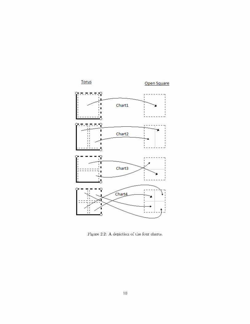
The sphere can be made into a manifold if we chart it using, for example, the typical θ and φ coordinates.Notice, however, that the domain of a coordinate map must be an open set (it has to be a homeomorphismafter all). This makes it impossible to put a global coordinate system on a sphere, more than one coordinatemap is necessary to cover it. Another interesting set of charts is stereographic projection, and yet anotherone is projecting the six hemispheres to six open disks.

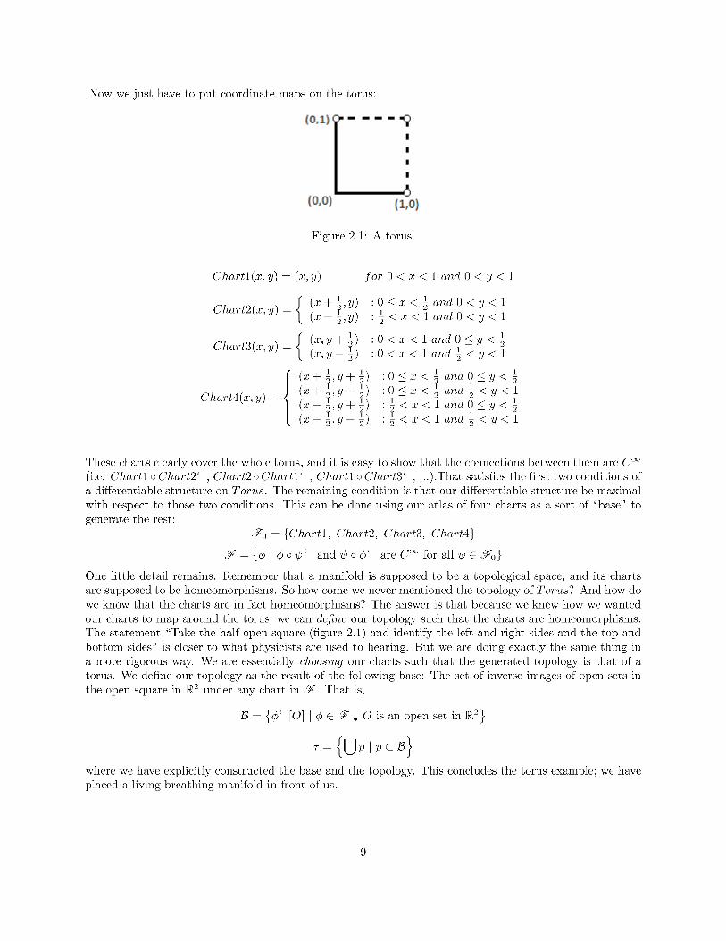
I’d like to present one very concrete example of a manifold before moving on. The torus as a topologicalspace is homeomorphic to a half-open square:

Torus = {(x, y) | 0 ≤ x < 1 • 0 ≤ y < 1}

8

Chapter 3

Tangent Space

3.1 What we need

When we’re doing calculus in regular old Rn, the notion of directional derivative is quite clear. A scalar

field, for example, would be a function f : Rn → R. Each n-tuple v of real numbers defines a directionalderivative operation, v ·∇f , where ∇ represents the primitive gradient operator ( ∂

∂x, ∂∂y, ∂∂z

). The derivative

of a path (γ : R → Rn) is also pretty simple, it’s just the component-wise derivative of the three component

functions that make up the path. Then if we want to look at the directional derivative of f along γ, we putthe two together: γ′ · ∇f . Manifolds require us to rethink these ideas.

It is not obvious how one would take a directional derivative of a real valued function on a manifold, or evenjust the derivative of a path. What we need is a coordinate-independent object that represents direction oftravel throughout the manifold. Let us state the problem more precisely. Consider a path in the manifoldand a real valued function on the manifold:

γ : R →M

f :M → R

How can we define the derivative of f along the path γ? Intuitively such a thing should exist; the spaceis locally euclidean after all. The composite function f ◦ γ would give us the values of f along the pathaccording to the path parameter. This is an R → R

n function, so we can take it’s derivative at a point andget an n-tuple of real numbers, (f ◦ γ)′. Such a derivative tells us how “fast” the path γ is traveling throughvalues of f. Of course the niceness of f and γ are needed to make this work out, but it seems like the speedat which this path goes through values of f sort of tells us which way it’s going and how fast. But the speedwe will get obviously depends on choice of f ; we need to get the character of f out of our definition, we wantthe derivative of the path itself. It makes sense to look at the directional derivative given by γ through anynice enough function on the manifold. That is, it makes sense to consider the object ( ◦ γ)′ where the “ ”can be filled in by any nice enough function.

There is a way of defining tangent vectors that directly uses paths. It actually defines tangent vectors asequivalence classes of paths on the manifold. We will not be doing this. Our definition will take less directadvantage of the path concept, but it will be more powerful. We will be utilizing the algebraic structure of

11

a set of nice functions.

3.2 Definitions

Let Fm,M denote the set of smooth functions on a manifold M that are defined on an open set containingm.

Fm,M = { f | (∃U | f : U → R • f ∈ C∞M • m ∈ U ∈ τM ) }

This set seems to have a very natural algebraic structure; it can be made into an algebra. This means ithas to have a group operation (“addition”), a multiplication, and a scalar field with a scaling operation.Two elements of this set f, g ∈ Fm can be added and multiplied by pointwise addition and multiplication offunctions. A real number a can scale a function f ∈ Fm in a similar pointwise way.

(f + g)(x) = f(x) + g(x)

(fg)(x) = f(x) · g(x)

(af)(x) = a · f(x)

It is not difficult to show that these operations produce things that are also members of Fm,M , nor is itdifficult to prove the needed properties of an algebra and more (commutativity, distributivity, associativity,identity, inverse). It should be known that the domain of a function produced after addition or multiplicationis the intersection of the domains of the two functions being added or multiplied. (Note: I have a confessionto make; this is not really the correct way to construct the algebra. Consider for example the additive inverseof some f ∈ Fm,M , f : U → R. The inverse should just be (−1)(f) (or −f). However upon addition wefind that f + (−1)(f) is not just the zero function, it is the zero function restricted to the domain U . Forfunctions to be equal they must have equal domains. For this reason and others, it makes a lot more sense toconstruct the algebra out of germs, equivalence classes of smooth functions that agree on some neighborhoodof m ∈M . Warner provides this treatment in his definition of tangent space, and it is very well done. I amchoosing to avoid these complications so as not to lose sight of the basic ideas. It is recommended that thereader who is already familiar with these concepts consult Warner for a fuller explanation).

An operator in our case would be a function from Fm,M to the real numbers, O : Fm,M → R. A linearoperator has the property O(af + bg) = a · O(f)+ b · O(g) for any f, g ∈ Fm,M , a, b ∈ R. An operator whichis a derivation-at-m has the property O(fg) = O(f) · g(m) + O(g) · f(m) for any f, g ∈ Fm,M . Operatorsalso have their own pointwise addition and scalar multiplication over the real numbers. For two operatorsO,P and a ∈ R

(O + P)(f) = O(f) + P(f)

(aO)(f) = a · O(f)

Definition 3.2.1. The tangent space of the manifold M at m ∈M , Tm,M , is the set of linear derivations-at-m on Fm,M . This is a vector space over the real numbers, with addition and scalar multiplication beingthe above defined operator operations.

Let us now make sure that our space behaves in the way we intended. If a ∈ R, let a denote the constantfunction of value a on the manifold. Clearly a ∈ Fm,M for any m ∈M .

Theorem 3.2.1. For any t ∈ Tm,M and c ∈ R, t(c) = 0.

12

Proof. c · t(1) = t(c · 1) = t(c) · 1(m) + t(1) · c(m) = t(c) · 1 + t(1) · c = t(c) + c · t(1)So c · t(1) = t(c) + c · t(1) so t(c) = 0

Theorem 3.2.2. For any f, g ∈ Fm,M such that f and g have the same value on some neighborhood U ofm, we have t(f) = t(g) for any t ∈ Tm,M .

Proof. Take f, g ∈ Fm such that f and g have the same value on the neighborhood U of m, and take anyt ∈ Tm,M . Let 1↾U denote the function 1 restricted to the domain U . Note that our hypothesis on f and gcan be written (1↾U ) · f = (1↾U ) · g.t((1↾U ) · f) = t(1↾U ) · f(m) + t(f) · (1↾U )(m) = t(1↾U ) · f(m) + t(f) = t(1↾U · g) = t(1↾U ) · g(m) + t(g) =t(1↾U ) · f(m) + t(g)where we have used f(m) = g(m). We established t(1↾U )·f(m)+t(f) = t(1↾U )·f(m)+t(g), so t(f) = t(g).

This basically says that a tangent vector at m only cares about purely local values of functions around m.If it wasn’t clear already, this theorem should make it clear that it makes a lot more sense to deal withan algebra consisting of germs of functions rather than actual functions. Nevertheless, we are happy to seetangent vectors work the way we wanted them to.

Now we may answer the original question. If γ : R →M is a smooth curve and γ(c) = m then we define thetangent vector to γ at c to be the operator t such that for f ∈ Fm,M ,

t(f) = (f ◦ γ)′(c)

We characterize the speed and direction at which a path is traveling through the manifold by the speed atwhich it travels through the values of smooth real-valued functions on the manifold. It is not difficult toshow that the definition above is in fact a linear derivation at m, and thus may be called a tangent vectorat m.

3.3 Coordinate Basis

Now let us consider the dimensionality of Tm,M for some manifold. Wald’s General Relativity (p17) does anice proof that the dimensionality of the tangent space is the same as the dimensionality of the manifold. Iwill not show this proof here, but the important part is that he does it by constructing a basis for Tm,M .I recommend Bishop and Goldberg (p52) for proofs about the basis. First, get a chart φ that has m in itsdomain (one should exist since the charts cover the manifold). Let {ti} be tangent vectors such that for anyf ∈ Fm,M ,

ti(f) =∂f ◦ φ←

∂xi

∣∣∣∣φ(m)

Since f maps from M to R and φ← maps from Rn to M , the object f ◦ φ← is from R

n to R. It is just thefunction f viewed in R

n through the eyes of the coordinate system φ. And the ti are the operators thatlook at functions through φ and take their derivatives in the directions of the coordinate axes. They form avery special basis called the coordinate basis. That they form a basis at all is an important theorem whoseproof I will not show, but it is in the references mentioned above. It is an excellent exercise to show, usingthe definitions we’ve provided, that the coordinate basis at a point consists of the tangent vectors to thecoordinate axes (coordinate axes are actual paths in the manifold).

13

We conclude this section by examining a property of tangent vectors that many physicists use to define theword “vector”. This is the transformation law that arises from the coordinate basis expansion of an arbitraryt ∈ Tm,M , and the chain rule. I like to express operators by using an underscore to show how they behave.For example the coordinate basis vector at m for the ith coordinate of a coordinate system φ is a map that

takes f ∈ Fm,M and spits out the number ∂(f◦φ←)∂xi

∣∣∣∣φ(m)

. My informal way of denoting this operation is

∂( ◦φ←)∂xi

∣∣∣∣φ(m)

. The underscore looks like a blank space where the operator is waiting to be fed a function in

Fm,M . Now take any t ∈ Tm,M . Let’s express it in the coordinate basis induced by the coordinate systemφ, and then try to get its expression in terms of the coordinate system ψ.

t =

n∑

i=1

ai∂( ◦ φ←)

∂xi

∣∣∣∣φ(m)

=n∑

i=1

ai∂( ◦ ψ← ◦ ψ ◦ φ←)

∂xi

∣∣∣∣φ(m)

=

n∑

i=1

ain∑

j=1

∂( ◦ ψ←)

∂xj

∣∣∣∣ψ(φ←(φ(m)))

∂(ψ ◦ φ←)j

∂xi

∣∣∣∣φ(m)

=

n∑

j=1

(n∑

i=1

ai∂(ψ ◦ φ←)j

∂xi

∣∣∣∣φ(m)

)∂( ◦ ψ←)

∂xj

∣∣∣∣ψ(m)

The superscript in (ψ ◦ φ←)j indicates the jth component function. So the new components in the ψcoordinate basis depend on the coordinate transformation (ψ ◦ φ←).

bj =

n∑

i=1

ai∂(ψ ◦ φ←)j

∂xi

∣∣∣∣φ(m)

t =

n∑

i=1

bi∂( ◦ ψ←)

∂xi

∣∣∣∣ψ(m)

This is the tangent vector transformation law.

14

Chapter 4

Cotangent Space

I read what four books had to say about this topic since it’s important to understand before getting intodifferential forms and tensors. Warner was the most general and the most concise, but I eventually chose tofollow Frankel’s approach. Schutz spent a lot of time on fiber bundles and tangent bundles in particular beforegetting into differential forms. His presentation of bundles was extremely good, but since my goal in thesenotes is to get to lie derivatives, I’m not doing bundles. Frankel doesn’t assume the reader’s familiarity withdual spaces. He takes care of the necessary math with good explanations, and then he defines differentialswith the tools he built. The only problem is that he doesn’t treat the more general definition first. So I’mgoing to start by presenting the general, formal definition of a differential up front. Then I’ll backtrack tothe beginning and build up to the specific kind of differential we’ll be using. For learning this the first time,Bishop and Goldberg chapter 2 was the best reading.

Take note that this discussion is limited to finite dimensional vector spaces. I don’t need the infinitedimensional results, and there are some serious differences. Also, the scalar field over which these vectorspaces lie is the field of real numbers. I didn’t have to do this, but it’s all we really need. It’s easy to makethe discussion general; just replace the word “real number” with “scalar” and replace R with F .

4.1 A Cold Definition

Consider a C∞ map ψ : M → N from one manifold to another. The differential of ψ at m ∈ M is a linearmap dψ : Tm,M → Tψ(m),N defined as follows. For any tangent vector t ∈ Tm,M , feeding it to the differentialshould give a tangent vector dψ(t) ∈ Tψ(m),N in the tangent space of the other manifold. This tangent vectordψ(t) is defined by how it acts on some g ∈ Fψ(m),N :

dψ(t)(g) = t(g ◦ ψ)

So the map ψ is used to view the function on N , g, as it appears on M through ψ’s eyes. This is then whatis fed to t. The notation dψ is actually incomplete; a good notation should indicate information about mand M (for example dψm,M ). But we’ll stick to crappy notation for now. Well that’s it for the definition, itdoesn’t really tell us much. We will come back to this definition more seriously in section 7.1. For now whatwe will be interested in is a special case of this definition where the second manifold, N , is actually just R.Let us go back to the beginning and make some sense of this.

15

4.2 Dual Space

Consider a vector space E over the real numbers. A linear function on a vector space E is a functionh : E → R such that for a, b ∈ R and v, w ∈ E, h(av + bw) = ah(v) + bh(w). The property of linearity isa pretty big deal here. Since it generalizes to any finite sum by induction, and we can expand any vectorv ∈ E into components of a basis {ej},

h(v) = h

n∑

j=1

ejvj

=

n∑

j=1

h(ej)vj

we see that the action of a linear function on a any vector in E is completely defined by what it does to onlythe vectors of a basis of E. This means we can just take any old basis {ej} of E, say what number eachh(ej) gives, and define h to be the “linear extension” of that.

So where do these linear functions live? They live in another vector space E∗ called the dual space of E. E∗

is just the set of all linear functions on E. Its elements are often called dual vectors. It has the pointwisevector addition and scalar multiplication of functions. So for a ∈ R, w1, w2 ∈ E∗, and any v ∈ E:

(a · w1)(v) = a · w1(v)

(w1 + w2)(v) = w1(v) + w2(v)

It’s easy to show that the dual space is a vector space. Now for any basis of E, {ei}, there is a correspondingbasis of E∗,

{σi}, defined by the linear extensions of:

σi(ej) = δij

It is not difficult to show that these form a basis for E∗. Something interesting happens when we feed avector v ∈ E to a basis dual vector σi.

σi(v) = σi

n∑

j=1

ejvj

=

n∑

j=1

σi(ej)vj =

n∑

j=1

δijvj = vi

So if σi is the dual basis vector corresponding to a basis vector ei, then feeding any v ∈ E to σi gives usv’s component along ei. Now we can find the basis expansion of an arbitrary dual vector w ∈ E∗ by justfeeding it a vector v ∈ E and using what we just found:

w(v) = w

n∑

j=1

vj ej

=

n∑

j=1

vjw(ej) =

n∑

j=1

σj(v)w(ej)

w =

n∑

j=1

w(ej) σj

This means that the component of w along σj is w(ej).

When we talk about a w ∈ E∗, we’re talking about a real valued function of an E-valued variable, v.

w(v), for v ∈ E

We can switch around our view of the real number w(v). Instead of focusing our attention on this particularw ∈ E∗, we can consider a particular v ∈ E. We can then see w(v) as a real valued function of an E∗-valuedvariable, w.

w(v), for w ∈ E∗

16

So what we’re really talking about is a v : E∗ → R such that for any w ∈ E∗,

v(w) = w(v)

We see that v ∈ E∗∗, it is a member of the dual space to the dual space of E. The map v 7→ v can be shownto be a 1-1 linear function from E to E∗∗. This makes the dual space of the dual space of a vector spaceisomorphic to the original vector space. This is no ordinary vector space isomorphism, however. This is anatural isomorphism. The real definition of natural isomorphism comes from category theory; the actualnatural isomorphism is the functor one can define from the entire category of n dimensional vector spacesto itself. There is no real need to get into the details of category theory, so can just be thought of as avector space isomorphism that is related only to the vector space structure, not any basis. For example, thedual space to a vector space is isomorphic to the vector space, but this isomorphism is not natural becauseit depends on choice of basis. Any n-dimensional vector space is isomorphic to R

n, but again there is anisomorphism for each choice of basis.

We could have also viewed the object w(v) in the following symmetric way: w(v) is a real valued functionof two variables, an E-valued variable v and an E∗-valued variable w. The map (v, w) 7→ w(v) is then ourdefinition of scalar product: < v,w >.

4.3 Cotangent Space

The tangent space at a point in a manifold, Tm,M is a vector space. The dual of this space, T ∗m,M , is calledthe cotangent space. We can define an element of the cotangent space at m by using a function f ∈ Fm,M .It is called the differential of f, df : Tm,M → R. For any v ∈ Tm,M , it is defined by

df(v) = v(f)

So taking a smooth real valued function f on the manifold and putting a d in front of it creates a functionthat feeds f to any tangent vector fed to it. This is obviously a linear function on Tm,M , so it must be inT ∗m,M . I find it helpful to resort to my underscore notation, which I explained in the previous section andin the appendix. In terms of the components of a tangent vector in a coordinate basis from a coordinatesystem φ,

df(v) = df

n∑

j=1

vj∂ ◦ φ←

∂xj

∣∣∣∣φ(m)

=

n∑

j=1

vj∂f ◦ φ←

∂xj

∣∣∣∣φ(m)

It’s nice to look at tangent vectors and their duals in terms of the underscore notation, in a coordinate basis.A vector, given components vj , is just the map

n∑

j=1

vj∂ ◦ φ←

∂xj

∣∣∣∣φ(m)

where the underscore is waiting to be fed a smooth function. And a dual vector, given a smooth function f ,is the map

n∑

j=1

j ∂f ◦ φ←

∂xj

∣∣∣∣φ(m)

where the underscore is waiting to be fed the components of a vector in the coordinate basis. This viewmakes it intuitively clear that the dual of the dual to the tangent space is naturally isomorphic to the tangentspace.

17

Let us now consider the differential of a coordinate function. Suppose (x1, ..., xn) are the coordinate functions(component functions, projections) of a coordinate system φ. First look at how dxi acts on the jth coordinatebasis vector:

dxi

(∂ ◦ φ←

∂xj

∣∣∣∣φ(m)

)=∂xi ◦ φ←

∂xj

∣∣∣∣φ(m)

= δij

Now we’re able to decompose the action of the differential on any tangent vector:

dxi

n∑

j=1

vj∂ ◦ φ←

∂xj

∣∣∣∣φ(m)

=

n∑

j=1

vj∂xi ◦ φ←

∂xj

∣∣∣∣φ(m)

=

n∑

j=1

vjδij = vi

The differential of the ith coordinate function just reads off the ith component of a tangent vector in thecoordinate basis! The

{dxi}then form a dual basis to the coordinate basis. That is, we can express any

linear function in terms of this dual basis expansion:

w =

n∑

j=1

w

(∂ ◦ φ←

∂xj

)dxj

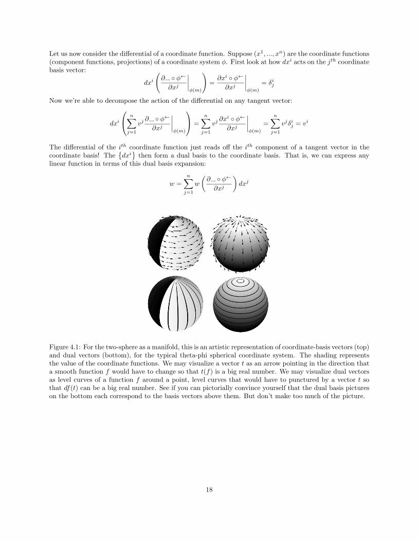
Figure 4.1: For the two-sphere as a manifold, this is an artistic representation of coordinate-basis vectors (top)and dual vectors (bottom), for the typical theta-phi spherical coordinate system. The shading representsthe value of the coordinate functions. We may visualize a vector t as an arrow pointing in the direction thata smooth function f would have to change so that t(f) is a big real number. We may visualize dual vectorsas level curves of a function f around a point, level curves that would have to punctured by a vector t sothat df(t) can be a big real number. See if you can pictorially convince yourself that the dual basis pictureson the bottom each correspond to the basis vectors above them. But don’t make too much of the picture.

18

Chapter 5

Tensors

This section will begin with more talk of linear functions on vector spaces. We will discuss matrix forms,multilinear functions, summation notation, tensor spaces, tensor algebra, natural isomorphisms leading todifferent interpretations of tensors, bases of tensor spaces and components of tensors, and transformationlaws. There will be a tiny bit of repetition of the previous section, because this is its ultimate generalization.I learned most of this material from Bishop and Goldberg chapter 2, which I highly recommend. For someonewho is very familiar with algebra (not me), I would recommend Warner. Schutz gives the typical physicsexplanation of tensors, which is a very bad explanation for a newcomer to the subject. Like the previoussection, I’m going to start with general mathematical concepts before applying them to our concrete exampleof a vector space, the tangent space. For my own reference, here is a list of topics I missed that I wouldlike to fill in someday: invariants, formal definition of a contraction, symmetric algebra, grassman algebra,determinant and trace, and hodge duality.

5.1 Linear Functions and Matrices

Let us expand our previous definition of linear function. A linear function f : V → W may now map fromone vector space V into another W so that for v1, v2 ∈ V and a ∈ R we have

f(v1 + v2) = f(v1) + f(v2)

f(av1) = af(v1)

Bijective linear functions are vector space isomorphisms. The set of linear functions from V to W forms avector space with pointwise addition of functions and pointwise scalar multiplication. There are a lot of nicethings we could prove about bases, dimensionality, null spaces, and image spaces. For this I refer the readerto Bishop and Goldberg pages 59-74, or a linear algebra book. I don’t have time to get that material writtenbut we’ll build up what we need.

It is still the case that we only have to define linear functions on basis elements to characterize them.Consider a linear function f : V → W , where dim(V )=dV and dim(W )=dW . Let {vi} be a basis of Vand {wα} a basis of W , where the indices run over the appropriate dimension. We introduce the hopefullyfamiliar summation convention, in which any index that appears twice is summed over. Let’s say that we’ve

19

determined the action of f on the basis vectors {vi}. Since f takes each of those to a particular vector inW , we will need dW different scalars to represent each f(vi) in the basis {wα},

f(vi) = aαi wα

The double-indexed object aαi is a dW by dV matrix, where α is the row index and i is the column index. ais called the matrix of f with respect to {vi} and {wα}. Notice that our designation of one index as “row”and the other as “column” is completely arbitrary. This is the point in our discussion where we make thatarbitrary choice, and any other remark about rows or columns will be with respect to this choice. Nowconsider any v ∈ V . Then f(v) is some w ∈W .

f(v) = f(vivi) = vif(vi) = viaαi wα = wαwα

where wα = aαi vi

The action of f is in fact determined by our grid of numbers aαi . We let this give us the definition ofmultiplication of a matrix by what we now deem to be a column matrix vi to give another column matrixwi. Let BV : V → R

dV be the function that takes any vector v ∈ V and gives the dV -tuple of componentsin the basis {vi}, and similarly for BW :W → R

dW . Let A : RdV → RdW represent matrix multiplication of

aαi by the tuples in RdV . The following diagram then sums up what we just showed:

We could define matrix multiplication in terms of the composition of operators, and we could prove distribu-tivity and associativity. I will not do this here.

Summation notation is pretty tricky. It should be noted that the types of sums being done depends on thecontext. For example viei is a sum of vectors, vector addition. But viwi is a sum of scalars, real numberaddition. Summation notation makes everyday tasks easy, but it also obscures some other things. Forexample, what do we really mean by “aαi ?” Is it a matrix? Or is it a number, the (α, i)th component of amatrix? Or is it the operator independent of any basis? Authors don’t seem to agree on the answer to thisquestion. Wald solves the problem by using latin indices for operators and greek indices for components in abasis. Here is my system: a is the operator, the function on the vector space(s). aαi is still the operator, butwith indices that indicate the structure of the operator if it were to be resolved in a basis. Contractions ofindices in this case are basis independent things done to operators. aαi is the (α, i)th component of a matrixin some basis, and contractions of these indices are actual sums.

5.2 Multilinear Functions

A function f : V1 × V2 →W is multilinear if it is linear in each individual variable. That is, for v1, y1 ∈ V1,v2, y2 ∈ V2, and a, b ∈ R

f(av1 + by1, v2) = af(v1, v2) + bf(y1, v2)

20

f(v1, av2 + by2) = af(v1, v2) + bf(v1, y2)

The function above is bilinear. The definition of multilinear generalizes to a function of n vectors,

f(v1, . . . , avi + byi, . . . , vn) = af(v1, . . . , vi, . . . , vn) + bf(v1, . . . , yi, . . . , vn)

Now suppose ν ∈ V ∗ and ω ∈W ∗, these are linear real-valued functions on the vector spaces V and W . Wecan form a bilinear function on V ×W by taking their tensor product. It is a function such that for v ∈ V

and w ∈W

ν ⊗ ω(v, w) = ν(v) · ω(w)

We can pointwise-add multilinear functions of a certain type to produce more multilinear functions. We canalso scalar multiply multilinear functions pointwise. Thus the set of multilinear functions on some vectorspaces V1, V2, . . . , Vn into W is a vector space. We denote this vector space by L(V1, . . . , Vn;W ).

5.3 Tensors

For a vector space V , the real-valued multilinear functions with any number of variables in V and V ∗ arecalled tensors over V . The tensor type is determined by the number of dual vectors it takes and the numberof vectors it takes, in that order. A multilinear function T : V ∗ × V × V → R for example is a type (1, 2)tensor. We always want to have the dual spaces come first in the list of variables, so we are not interestedin a map V × V ∗ → R. That map is already taken care of by the equivalent one with permuted variables,V ∗ × V → R. The set of tensors of a particular type form a vector space called a tensor space over V , andwe call that space T ij (V ) for tensors of type (i, j) over V . Addition and scalar multiplication are pointwise

for functions. So for A,B ∈ T ij (V ), a ∈ R, v1, . . . vj ∈ V , and w1, . . . , wi ∈ V ∗

(A+B)(w1, . . . , wi, v1, . . . , vj) = A(w1, . . . , wi, v1, . . . , vj) +B(w1, . . . , wi, v1, . . . , vj)

(aA)(w1, . . . , wi, v1, . . . , vj) = aA(w1, . . . , wi, v1, . . . , vj)

A tensor of type (0, 0) is defined to be a scalar, T 00 (V ) = R. Notice that we are treating the vector space V

as if it is V ∗∗. The natural isomorphism we talked about is taken very seriously. People hop between V andV ∗∗ so effortlessly that we just use V to refer to both.

So T ij (V ) is the set of multilinear real-valued functions on V ∗ i times and on V j times. In particular, T 11 (V )

is the set of multilinear maps on V ∗ × V . If we take a v1 ∈ V and a w1 ∈ V ∗, we can form an element ofT 11 (V ) using the tensor product we defined earlier, v1 ⊗ w1 ∈ T 1

1 (V ). Can we form any element of T 11 (V ) in

this way? The answer is no, if the dimension of V is at least 2. Because for dimension 2 for example, we couldtake another linearly independent v2 ∈ V and w2 ∈ V ∗. Then if we were able to formulate v1 ⊗w1 + v2 ⊗w2

as some v⊗ w, we could partially evaluate the resulting equation, v1 ⊗w1 + v2 ⊗w2 = v⊗ w, and we wouldbe forced to violate linear independence. We will soon see how we can form a basis for tensor spaces, butlet’s get some algebra out of the way first.

We should expand our first definition of tensor product to work for tensors of any type. The tensor productof an (i, j) tensor A with an (r, s) tensor B is an (i + r, j + s) tensor that takes in the combined variablesof A and B, feeds them respectively to A and B to get two real numbers, and then spits out the product.That is, for a set of wa ∈ V ∗ and vb ∈ V

(A⊗B)(w1, . . . , wi+r, v1, . . . , vj+s) = A(w1, . . . , wi, v1, . . . , vj) ·B(wi+1, . . . , wi+r, vj+1, . . . , vj+s)

Now we can state associative and distributive laws for tensor product, they are easy to prove:

(A⊗B)⊗ C = A⊗ (B ⊗ C)

21

A⊗ (B + C) = A⊗B +A⊗ C

(A+B)⊗ C = A⊗ C +B ⊗ C

We already have some examples of tensor spaces. A vector space V ∗∗ (which we identify with V ) containslinear functions on V ∗, so it is just the tensor space T 1

0 (V ). The dual vector space contains linear functionson V , so it is just the tensor space T 0

1 (V ).

To resolve the elements of a tensor space T rs (V ) in a particular basis, we need a basis of V , {ei}, and abasis of V ∗,

{σj}. Just like a linear function is completely determined by its action on a basis and its linear

extension, a multilinear function is determined by its action on the basis{ei1 ⊗ . . .⊗ eir ⊗ σj1 ⊗ . . .⊗ σjs

}

(for all permutations of the indices) and its multilinear extension. If we can prove that the action ofA ∈ T rs (V ) on

{ei1 ⊗ . . .⊗ eir ⊗ σj1 ⊗ . . .⊗ σjs

}completely determines A, then we can express A in terms

of the proposed basis and we know that it spans the space. Linear independence is easy to prove usinginduction. So we can show that

{ei1 ⊗ . . .⊗ eir ⊗ σj1 ⊗ . . .⊗ σjs

}is a basis for T rs (V ). Let

Ai1...irj1...js= A(σi1 , . . . , σir , ej1 , . . . , ejs)

To feed A an arbitrary set of variables we need a set of r dual vectors ωa ∈ V ∗ and a set of s vectors νb ∈ V .These can expressed in their components in each basis:

ωa = wak σk

νb = vlbel

And just because we’ll need it soon, remember that basis vectors and dual vectors can be used to read offcomponents of dual vectors and vectors:

wak = ek(ωa)

vlb = σl(νb)

Now we can feed them to A,

A(ω1, . . . , ωr, ν1, . . . , νs) = A(w1i1σi1 , . . . , wrir σ

ir , vj11 ej1 , . . . , v

jss ejs)

and use multilinearity:

= (w1i1. . . wrir )(v

j11 . . . vjss )A(σi1 , . . . , σir , ej1 , . . . , ejs)

= (w1i1. . . wrir )(v

j11 . . . vjss )Ai1...irj1...js

= Ai1...irj1...js(ei1(ω

1) . . . eir (ωr))(σj1(ν1) . . . σ

js(νs))

=[Ai1...irj1...js

(ei1 ⊗ . . .⊗ eir ⊗ σj1 ⊗ . . .⊗ σjs)](ω1, . . . , ωr, ν1, . . . , νs)

And we finally have A in terms of the basis:

A = Ai1...irj1...js(ei1 ⊗ . . .⊗ eir ⊗ σj1 ⊗ . . .⊗ σjs)

Notice that the dimension of the tensor space T rs (V ) must then be dim(V )r+s

5.4 Interpretations of Tensors

Consider a tensor A ∈ T 11 (V ). There are a couple of ways to view this object. One could see it for what

it is, a multilinear map from V ∗ × V to the real numbers. This isn’t always the geometrically meaningful

22

interpretation. If we take a dual vector w ∈ V ∗ and we feed that to A, then we’ve only partially evaluatedit. A still has its mouth open, waiting to be fed a vector. So after feeding only w to A we’re left with alinear map V → R, which is a dual vector. We can name this function A1 : V ∗ → V ∗, and it is the mappingw 7→ (v 7→ A(w, v)). Similarly we could have taken a v ∈ V , fed v to A, and left it hungry for a dual vector.That would have left us with a map V ∗ → R, which is a vector (in the naturally isomorphic sense). Wename that function A2 : V → V and it is the mapping v 7→ (w 7→ A(w, v)). These are three ways to interpretthe same action: producing a real number from two objects. We consider the different mappings A, A1, andA2 to be the same without any choice of basis; so they are naturally the same. Formally we would say thatT 11 (V ), L(V ;V ), and L(V ∗;V ∗) are naturally isomorphic vector spaces.

These interpretations translate over to different designations of rows and columns once A is resolved insome basis

{ei ⊗ σj

}. Higher rank tensors analogously have multiple interpretations, there are more kinds

of interpretations for higher ranks. In practical situations, people treat naturally isomorphic spaces as thesame space without making a fuss over it. Even though different interpretations of the same tensor arestrictly different functions, people mix all of the different mappings into one “index structure”. So when wesay gµν we are referring to all of the interpretations mushed into one object. Once indices are contracted ina particular way, like gµνx

µ, we pick one interpretation (in this case the V → V ∗ type).

I’d like to do an example of a tensor interpretation with scalar products, before I end this. The scalarproduct operation, mentioned at the end of section 4.2, takes a vector and a dual vector and gives backa real number. It does this in a bilinear way, which makes it a tensor <,>: V ∗ × V → R. That’s oneinterpretation, <,>∈ T 1

1 (V ). What about <,>1: V∗ → V ∗? Well if we feed the scalar product a dual vector

w ∈ V ∗, it’s still waiting to be fed a vector. The map we are left with wants to take the vector we give itand feed it to w, by definition of scalar product. The remaining map must then be w itself. Okay how about<,>2: V → V ? Feed <,> a vector v ∈ V , and it is left hungry for a dual vector. When the remainingmap is fed a dual vector, it just feeds that to v and gives us the result. The remaining map must then be vitself by definition. So <,>1 and <,>2 are identity maps. The components of <,> in a basis

{ei ⊗ σj

}are

<,>ij=< σi, ej >= δij . It’s a Kronecker delta in any basis.

We could talk about tensor transformation laws in terms of vector transformation laws completely abstractly,without using our tangent space. But it’s time we head back home to the manifold; just know that the resultsconcerning transformation laws for tensors over a tangent space are derivable in general. It’s more instructiveand practical to get the transformation laws through the concrete example of tensor spaces over a tangentspace.

5.5 Back on the Manifold

The vector space we’ve been interested in is the tangent space at a point m in a manifold M , Tm,M . Thetensor spaces we are interested in are then T rs (Tm,M ). Let φ, ψ be coordinate systems with m ∈ M in theirdomain. Let the component functions of φ be x1, . . . , xn :M → R, where n is the dimension of the manifold.Let the component functions of ψ be y1, . . . , yn. Let t ∈ Tm,M be a tangent vector at m, and let φti representits components in the φ coordinate basis, and ψti its components in the ψ coordinate basis.

t = φti∂ ◦ φ←

∂xi

∣∣∣∣φ(m)

t = ψti∂ ◦ ψ←

∂xi

∣∣∣∣ψ(m)

23

At the end of section 3, we obtained the tangent vector transformation law using chain rule. We did this byexpressing one coordinate basis in terms of another.

∂ ◦ φ←

∂xi

∣∣∣∣φ(m)

=∂ ◦ ψ←

∂xj

∣∣∣∣ψ(m)

∂(ψ ◦ φ←)j

∂xi

∣∣∣∣φ(m)

ψtj = φti∂(ψ ◦ φ←)j

∂xi

∣∣∣∣φ(m)

Now we’re going to use the tangent vector transformation law to obtain the transformation law for the dualspace. First we name the components of the cotangent vector w ∈ T ∗m,M in terms of the dual bases to thecoordinate bases of φ and ψ.

w = φwi dxi

w = ψwi dyi

We want to express the{dxi}basis in terms of

{dyi}. Look at the values of dxi on the ψ coordinate basis:

dxi

(∂ ◦ ψ←

∂xj

∣∣∣∣ψ(m)

)= dxi

(∂(φ ◦ ψ←)k

∂xj

∣∣∣∣ψ(m)

∂ ◦ φ←

∂xk

∣∣∣∣φ(m)

)

=∂(φ ◦ ψ←)k

∂xj

∣∣∣∣ψ(m)

∂xi ◦ φ←

∂xk

∣∣∣∣φ(m)

=∂(φ ◦ ψ←)k

∂xj

∣∣∣∣ψ(m)

δik

=∂(φ ◦ ψ←)i

∂xj

∣∣∣∣ψ(m)

Then look at the values of dyk ∂(φ◦ψ←)i

∂xk

∣∣∣∣ψ(m)

on the ψ coordinate basis:

[∂(φ ◦ ψ←)i

∂xk

∣∣∣∣ψ(m)

dyk

](∂ ◦ ψ←

∂xj

∣∣∣∣ψ(m)

)=∂(φ ◦ ψ←)i

∂xk

∣∣∣∣ψ(m)

∂yk ◦ ψ←

∂xj

∣∣∣∣ψ(m)

=∂(φ ◦ ψ←)i

∂xk

∣∣∣∣ψ(m)

δkj

=∂(φ ◦ ψ←)i

∂xj

∣∣∣∣ψ(m)

They have the same values on the ψ coordinate basis, so they must be the same dual vector. Having expressed{dxi}in terms of

{dyi}, we may then relate the components of w in the different bases.

dxi = dyj∂(φ ◦ ψ←)i

∂xj

∣∣∣∣ψ(m)

ψwi =φwj

∂(φ ◦ ψ←)j

∂xi

∣∣∣∣ψ(m)

How do we find the transformation law for an arbitrary tensor? The hardest part is actually over, this oneis easy. I’ll do an example with a (1, 2) type tensor, A ∈ T 1

2 (Tm,M ). Remember from section 5.3 that the

24

components of A : V ∗ × V × V → R in a basis

{∂ ◦ψ←

∂xi

∣∣∣∣ψ(m)

⊗ dyj ⊗ dyk

}are

ψAijk = A

(dyi,

∂ ◦ ψ←

∂xj

∣∣∣∣ψ(m)

,∂ ◦ ψ←

∂xk

∣∣∣∣ψ(m)

)

Now we just use the vector and dual vector transformation laws that we got.

= A

(∂(ψ ◦ φ←)i

∂xa

∣∣∣∣φ(m)

dxa,∂(φ ◦ ψ←)b

∂xj

∣∣∣∣ψ(m)

∂ ◦ φ←

∂xb

∣∣∣∣φ(m)

,∂(φ ◦ ψ←)c

∂xk

∣∣∣∣ψ(m)

∂ ◦ φ←

∂xc

∣∣∣∣φ(m)

)

Then we can just use multilinearity to take out the scalar factors, and we’re left with the φ coordinate basiscomponents of A:

ψAijk = φAabc

(∂(ψ ◦ φ←)i

∂xa

∣∣∣∣φ(m)

∂(φ ◦ ψ←)b

∂xj

∣∣∣∣ψ(m)

∂(φ ◦ ψ←)c

∂xk

∣∣∣∣ψ(m)

)

And that is our tensor transformation law. Applying this simple procedure to any tensor gives its tensortransformation law. Actually if one is not interested in rigorously setting up the geometry, one can deal onlywith the transformation laws. In fact, some people have no idea what manifolds or tangent spaces are, butthey can still do highly geometrical physics because they understand transformation laws.

25

Chapter 6

Fields

This discussion follows the treatment of Bishop and Goldberg in chapter three, and it draws informationfrom Schutz. If I were to provide a treatment of differential forms, this would be the time to do it. But I’mnot going to treat them yet since they are a huge subject of their own and I’m currently in a poor positionto be writing about them. This section is missing examples of solving for integral curves, so if you’re notalready familiar with them please try to do some problems yourself.

6.1 Vector Fields

A vector field on a chunk of a manifold should be an object that assigns to each point in the manifold avector, an element of the tangent space there. A vector field X on an open D ⊂ M is a function such thatfor any m ∈ D, we get some X(m) ∈ Tm,M . Remember that a vector in a tangent space at m is actually alinear derivation-at-m, an operator defined by the way it acts on smooth functions around m. So a vectorfield returns a particular one of these operators at each point in D ⊂M . This gives us another way to view(or define) a vector field. Consider a smooth function f ∈ Fm,M defined on some open W ⊂ M . Just asacting a vector on f gives a real number, we can consider acting a vector field on f to give a real number ateach point. The vector field thus gives back some other function defined on dom(f) ∩ dom(X).

(X(f))(m) = (X(m))(f) for all m ∈ dom(f) ∩ dom(X)

Although the different ways of looking at the vector field, X and X, are strictly different objects, we glidebetween the different interpretations naturally enough to think of them as one object. I don’t like this, Iprefer that it’s clear which function we’re talking about. We might like our definition of vector fields tobe analogous to our definition of vectors. In that case we could have directly defined them as operators onsmooth real valued functions to real valued functions that are linear and obey a product rule.

We already defined the coordinate basis of a coordinate system φ at some point m in the coordinate sys-

tem’s domain U as the basis

{∂( ◦φ←)∂xi

∣∣∣∣φ(m)

for i < dimension

}. The mapping of m ∈ U to the vector

∂( ◦φ←)∂xi

∣∣∣∣φ(m)

produces the ith coordinate basis vector field ∂i. To make our notation of ∂i complete we

26

would need to know what coordinate system we’re talking about, so we may use φ∂i if the need arises. Nowour vector field X may be expressed in terms of the coordinate basis vector fields:

X = Xi∂i

where the Xi are functions on the manifold Xi : dom(φ) ∩ dom(X) → R, what we call the componentfunctions of the vector field (note that the multiplication that appears above is the pointwise multiplicationof a scalar function by a field of operators). This expansion into components works because at each m ∈dom(φ) ∩ dom(X), we may expand X(m) in terms of the coordinate basis there. The actual componentsXi are X(xi) where xi are the coordinate functions that make up φ:

X(xi) = (Xj∂j) (xi) = Xj ∂j(x

i) = Xi

What does it mean for a vector field to be smooth? A vector field is C∞ (smooth) if for any smooth realvalued function f on the manifold the function X(f) is also smooth. If a vector field is smooth then itscomponents in a coordinate system must also be smooth. This is because the components are X(xi) andthe xi are obviously smooth functions. Does the converse hold? Suppose the components of a vector fieldare smooth in every coordinate system on a manifold. Take any smooth f : W → R on the manifold. Thequestion to ask is whether X(f) is a smooth function for sure. Well at any point in W ⊂ M there shouldbe some coordinate system ψ : U → R

n with m ∈ U . The function X(f) in this coordinate system has a

domain D ∩ U ∩W and looks like Xi ψ∂i(f). Since the Xi are smooth functions and the ψ∂i are smoothvector fields it is clear that X(f) is smooth. So a vector field smooth iff it’s components are smooth in allcoordinate systems.

6.2 Tensor Fields

A tensor field should assign a tensor to each point in some chunk of the manifold. A tensor field T oftype (r, s) on some open subset D of the manifold is a function such that for every m ∈ D we get someT (m) ∈ T rs (Tm,M ). Just like there were multiple ways to define a vector field, there is another kind ofmapping that we can use to talk about a tensor field. But before we talk about that we need to understanddual vector fields. A vector field is clearly just a (1, 0) type tensor field. A dual vector field is just a (0, 1)type tensor field. A dual vector field Y : D → T 0

1 (Tm,M ) can be thought of as function that takes vectorfields to real valued functions. That is, we may consider the alternative mapping Y which takes a vectorfield and gives a function defined by

(Y (X))(m) = Y (m)(X(m)) for m ∈ dom(X) ∩ dom(Y )

Just like vector fields, these can be expanded in a basis at each point. The dual basis we’ve been talkingabout for T ∗m,M is denoted in a slightly misleading way,

{dxi}, where xi are the coordinate functions of

some coordinate system φ. A better notation, which I will now switch to using, is{dxi(m)

}. This indicates

that we’re talking about the differential of the smooth function xi at a particular m ∈ M . We’re going toreserve the old notation for a field. We let dxi : dom(φ) → T 0

1 (Tm,M ) refer to the tensor field defined bydxi(m) = dxi(m). Now we can talk about the components of a dual vector field, which can be expanded in acoordinate basis field:

Y = Yidxi

where the Yi are real-valued functions on dom(Y )∩ dom(φ) and the sum and products seen above are of thepointwise function type. Actually the Yi are just Y (φ∂i), since

Y (φ∂i) = Yjdxj(φ∂i) = Yi

27

Again, in practical situations nobody bothers with the difference between Y and Y ; I’m just more comfortablepointing it out when we’re doing this for the first time.

Tensors are multilinear functions on vectors and dual vectors, so a tensor field gives us a multilinear functionon the tangent vectors and cotangent vectors at each point. Thus if we have a tensor field T , we can considerthe function T that acts on vector fields and dual vector fields (ω1, . . . , ωr, ν1, . . . , νs) to produce real-valuedfunctions defined by

T (ω1, . . . , ωr, ν1, . . . , νs) (m) = T (m)(ω1(m), . . . , ωr(m), ν1(m), . . . , νs(m))

Tensor fields also have components in a basis. To express them this we way could define a “super tensorproduct” that acts on tensor fields. We can define the tensor field it makes out of tensor fields T and U by

(T ⊠ U)(m) = T (m)⊗ U(m) for m ∈ dom(T ) ∩ dom(U)

We may then express the tensor field T in terms of component functions, T i1...irj1...js, on a coordinate basis for

φ with coordinate functions xi:

T = T i1...irj1...js∂i1 ⊠ . . .⊠ ∂ir ⊠ dxj1 ⊠ . . .⊠ dxjs

The component functions can again be expressed as T i1...irj1...js= T (dxi1 , . . . , dxir , ∂j1 , . . . , ∂js)

What does it mean for a tensor field to be smooth? We already said that a vector field is smooth if feedingit any smooth function produces a smooth function. We then showed that this was equivalent to havingall the components of a vector field be smooth in every coordinate basis. Let’s see if we can say similarthings about tensor fields. A (0, 1) type tensor field, a dual vector field, is smooth (C∞) if feeding it anysmooth vector field produces a smooth function. An (r, s) type tensor field is smooth if feeding it r smoothdual vector fields and s smooth vector fields produces a smooth function. We now obtain similar statementsabout the smoothness of component functions. We will summarize them below. Consider a vector field X,a dual vector field Y , and an (r, s) type tensor field T:

X ∈ C∞ =⇒ Xi ∈ C∞ in any coordinate system because Xi = X(xi) and xi ∈ C∞

Xi ∈ C∞ in any coordinate system =⇒ X ∈ C∞ because X = Xi∂i and ∂i ∈ C∞

Y ∈ C∞ =⇒ Yi ∈ C∞ in any coordinate system because Yi = Y (∂i) and ∂i ∈ C∞

Yi ∈ C∞ in any coordinate system =⇒ Y ∈ C∞ because Y = Yidxi and dxi ∈ C∞

T ∈ C∞ =⇒ T i1...irj1...js∈ C∞ in any coordinate system because T i1...irj1...js

= T (dxi1 , . . . , dxir , ∂j1 , . . . , ∂js)

and dxi1 , . . . , dxir , ∂j1 , . . . , ∂js ∈ C∞

T i1...irj1...js∈ C∞ in any coordinate system =⇒ T ∈ C∞ because T = T i1...irj1...js

∂i1 ⊠ . . .⊠ ∂ir ⊠ dxj1 ⊠ . . .⊠ dxjs

and ∂i1 , . . . , ∂ir , dxj1 , . . . , dxjs ∈ C∞

6.3 Integral Curves

An integral curve γ... R →M of a vector field X is a path in the manifold whose tangent everywhere is the

value of the field. That is, γ is an integral curve of X if ( ◦ γ)′ = X ◦ γ (hidden in this statement is therequirement that ran(γ) ⊂ dom(X)). We say that the integral curve “starts at” m if γ(0) = m. It shouldbe clear that the definition of integral curve has nothing to say about starting point. So what happens

28

when we reparameterize the curve? Take an integral curve γ defined on the real interval Ka, bJ. Consider areparametrization of γ’s variable, r :Kc, dJ→Ka, bJ. Then ( ◦ γ ◦ r)′ = ( ◦ γ) ◦ r · r′. If we had r′ = 1, aconstant 1 function, then we’d have ( ◦γ◦r)′ = ( ◦γ)′◦r = X ◦γ◦r. The fact that ( ◦(γ◦r))′ = X ◦(γ◦r)tells us that the reparameterized curve, γ ◦ r, is also an integral curve. When is r′ = 1? This tells us that wecan translate the parameter of an integral curve and we’ll still have an integral curve. It also tells us thatspecifying the value of an integral curve at one point completely determines it. (Well, almost. Restrictingthe domain of an integral curve specified in this way does also make an integral curve. But we often justwant the “longest” curve we can get.)

Suppose that someone hands you a vector field and asks you for the integral curve that starts at a particularpoint in your manifold. To solve this problem, you reach into your atlas and grab an appropriate coordinatesystem φ with coordinate functions xi. Let us express the requirement that ( ◦ γ)′ = X ◦ γ in terms of φ.For s ∈ dom(γ):

( ◦ γ)′(s) = ( ◦ φ← ◦ φ ◦ γ)′(s) =∂ ◦ φ←

∂xj

∣∣∣∣φ(γ(s))

· (φ ◦ γ)j ′(s) = (∂j ◦ γ)(s) · (xj ◦ γ)′(s)

( ◦ γ)′ = (xj ◦ γ)′ · (∂j ◦ γ)

X ◦ γ = (Xj∂j) ◦ γ = (Xj ◦ γ) · (∂j ◦ γ)

The requirement to be an integral curve is then (xj ◦ γ)′ · (∂j ◦ γ) = (Xj ◦ γ) · (∂j ◦ γ). For every s ∈ dom(γ)and γ(s) ∈ dom(φ), (∂j ◦γ)(s) is a basis vector. So by requiring equality of vector components, the conditionbecomes a system of differential equations:

(xj ◦ γ)′ = Xj ◦ γ

This says that the derivative of the jth component of γ as viewed through φ is equal to the jth componentof the vector field at each point in the path. It is a system of first order ordinary differential equations. Thestarting point gives us the initial conditions so that it has a unique solution for xj ◦ γ (again, unique up toa restriction of the domain). It could be that dom(φ) does not cover dom(X). In that case we’d solve thedifferential equations for several coordinate systems and glue the pieces together.

I’m now going to skip a lot of differential equation theory. I’ve already skipped some by stating withoutproof that the system of equations above has a unique solution. I’m going to skip some powerful theoremsabout how big the domains and ranges of our integral curves could be, the reason being that they are toomathematical for what I want to get to right now. The bottom line is that any integral curve for a smoothvector field defined on all of a compact manifold can have its domain extended to all of R. Any vector fieldwith the property that all its integral curves can be extended to R is called complete.

6.4 Flows

Flows add no new information to what integral curves give us; they are just a different way of looking at thesame thing. If you’re standing in a vector field, you can travel along an integral curve by just walking alongthe arrows you’re standing on with the appropriate speed. So we have one point in the manifold (say m),some “time” t passes, and then we’re at another point in the manifold (say p). A particular integral curveis generated once we pick an m, it maps each t to a p (the integral curve starting at m). Similarly, part of aflow is generated when we pick a particular t, we get something that maps each m to p. The whole flow isthe object that produces a map from the m’s to the p’s for each choice of t. So the flow is one object that

29

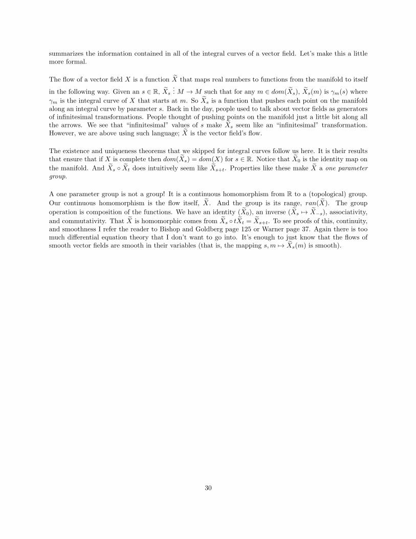
summarizes the information contained in all of the integral curves of a vector field. Let’s make this a littlemore formal.

The flow of a vector field X is a function X that maps real numbers to functions from the manifold to itself

in the following way. Given an s ∈ R, Xs

... M →M such that for any m ∈ dom(Xs), Xs(m) is γm(s) where

γm is the integral curve of X that starts at m. So Xs is a function that pushes each point on the manifoldalong an integral curve by parameter s. Back in the day, people used to talk about vector fields as generatorsof infinitesimal transformations. People thought of pushing points on the manifold just a little bit along allthe arrows. We see that “infinitesimal” values of s make Xs seem like an “infinitesimal” transformation.However, we are above using such language; X is the vector field’s flow.

The existence and uniqueness theorems that we skipped for integral curves follow us here. It is their resultsthat ensure that if X is complete then dom(Xs) = dom(X) for s ∈ R. Notice that X0 is the identity map on

the manifold. And Xs ◦ Xt does intuitively seem like Xs+t. Properties like these make X a one parametergroup.

A one parameter group is not a group! It is a continuous homomorphism from R to a (topological) group.

Our continuous homomorphism is the flow itself, X. And the group is its range, ran(X). The group

operation is composition of the functions. We have an identity (X0), an inverse (Xs 7→ X−s), associativity,

and commutativity. That X is homomorphic comes from Xs ◦ tXt = Xs+t. To see proofs of this, continuity,and smoothness I refer the reader to Bishop and Goldberg page 125 or Warner page 37. Again there is toomuch differential equation theory that I don’t want to go into. It’s enough to just know that the flows ofsmooth vector fields are smooth in their variables (that is, the mapping s,m 7→ Xs(m) is smooth).

30

Chapter 7

Lie Derivatives

This section attempts to combine the intuitive motivation of Schutz, the computational practicality of Bishopand Goldberg, and the mathematical rigor of Warner. Some of the terminology is my own. I’m going todo most of the discussion on Lie derivatives of vector fields, to avoid cluttering the calculations. Forms andother tensor fields come from vectors anyway, and it will not be too hard to generalize at the end. The usualnotation for evaluating a function a point, “f(x),” fails us here; there is just way too much going on. Tomake calculations easier on the eyes I’ll be using the alternative notation, “〈f | x〉”.

7.1 Dragging

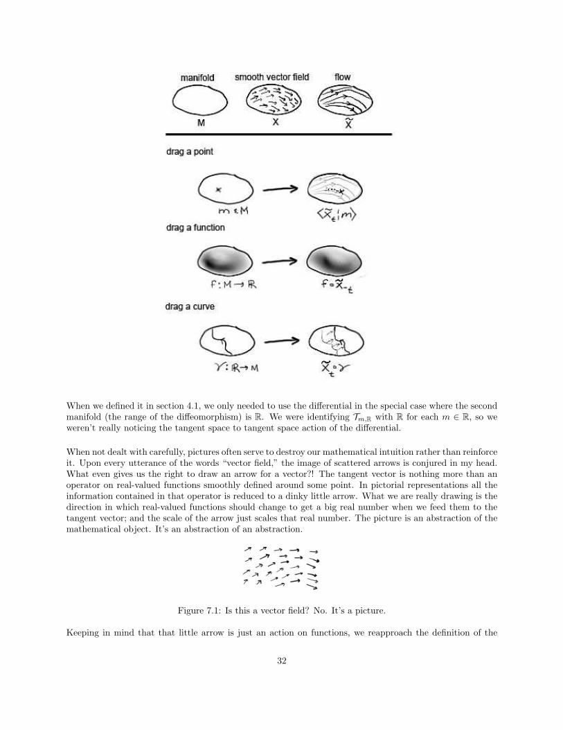
Good terminology can go a long way when it comes to visualizing advanced concepts. Here we introduce thenotion of Lie dragging. In section 6.4 we examined the one parameter group X made from the C∞ vectorfield X. Since each Xt has an inverse, X−t, and both are smooth functions from the manifold to itself, we

know that each Xt is a diffeomorphism. We may use it to take one point in the manifold, m, to anotherpoint along an X integral curve, 〈Xt | m〉. We will call this procedure “Lie dragging m along the vector fieldX.” The amount of dragging being done is given by the parameter t.

We can drag a real-valued function f... M → R in the following way. At each point we want the value of the

dragged function to be the value of the function pushed forward along the integral curves of X, so we lookbackwards by parameter amount t and return the function’s value there. The Lie dragged function is thenf ◦ X−t.

We can drag a curve γ : R → M by simply dragging the points in the range of the curve. The Lie draggedcurve along X is then Xt ◦ γ.

Now this one is the whopper. How can we Lie drag a vector field? We need a way to take all the vectorsfrom some vector field Y along the integral curves of the C∞ vector field X. That is, we need a way ofknowing what a vector looks like in a foreign tangent space, given that we used the diffeomorphism Xt totake it there. Remember that cold definition in section 4.1? This is a job for the differential map; it’s timeto understand it.

31

When we defined it in section 4.1, we only needed to use the differential in the special case where the secondmanifold (the range of the diffeomorphism) is R. We were identifying Tm,R with R for each m ∈ R, so weweren’t really noticing the tangent space to tangent space action of the differential.

When not dealt with carefully, pictures often serve to destroy our mathematical intuition rather than reinforceit. Upon every utterance of the words “vector field,” the image of scattered arrows is conjured in my head.What even gives us the right to draw an arrow for a vector?! The tangent vector is nothing more than anoperator on real-valued functions smoothly defined around some point. In pictorial representations all theinformation contained in that operator is reduced to a dinky little arrow. What we are really drawing is thedirection in which real-valued functions should change to get a big real number when we feed them to thetangent vector; and the scale of the arrow just scales that real number. The picture is an abstraction of themathematical object. It’s an abstraction of an abstraction.

Figure 7.1: Is this a vector field? No. It’s a picture.

Keeping in mind that that little arrow is just an action on functions, we reapproach the definition of the

32

differential. Consider the diffeomorphism ψ :M →M . dψ should take us from Tm,M to T〈ψ | m〉,M using ψ.

For some v ∈ Tm,M , 〈dψ | v〉 is just an action on functions. It makes perfect sense to take whatever function isfed to it, drag it backwards using ψ so the smooth part is back at m, and then feed that to v. This intuitivelytakes the action on functions (vector) in one place to the same action on functions (vector) dragged forwardusing ψ, by simply dragging back all the functions using ψ! Indeed we defined 〈〈dψ | v〉 | f〉 = 〈v | f ◦ ψ〉 forf ∈ F〈ψ | m〉,M (remember that dragging the function forward would have used ψ←).

So to Lie drag a vector v ∈ Tm,M along the vector field X by amount t we just feed it to the differential:

〈dXt | v〉. We can Lie drag a vector field Y along the vector field X in the following way. At each point wewish to look back by integral curve parameter amount t and return the vector there. However we need thatvector to be in the right tangent space, otherwise the result would not really be a vector field (it would besome horrible function that returns a foreign tangent vector at each point). So we drag it along by t using

the differential. The Lie dragged vector field is then dXt ◦ Y ◦ X−t.

(Note: We noted before that the notation dψ was incomplete, that dψm,M would be more appropriate. I’mjust using dψ as if it worked for all points, like a mapping between tangent bundles instead of just betweentangent spaces. Set-theoretically, I’m taking dψ to be the union of all the dψm,M for m ∈ dom(ψ))

In case you are still not convinced that this was the “right way” to define the dragging of a vector field, Ihave one more trick up my sleeve. Let us consider what happens to the integral curves of a vector field whenwe Lie drag it along another vector field. Consider smooth vector fields X and Y (we will drag Y along Xby amount t). Let γ represent arbitrary integral curves of Y . Let γ∗ represent arbitrary integral curves of

the dragged field, dXt ◦ Y ◦ X−t. We are searching for a relationship between the γ’s and the γ∗’s.

Each γ is a solution to:Y ◦ γ = ( ◦ γ)′

And each γ∗ is a solution to:

dXt ◦ Y ◦ X−t ◦ γ∗ = ( ◦ γ∗)′

〈dXt ◦ Y ◦ X−t ◦ γ∗

| s〉 = 〈( ◦ γ∗)′ | s〉

∀ f ∈ F〈γ∗ | s〉,M 〈〈dXt | 〈Y | 〈X−t ◦ γ∗

| s〉〉〉 | f〉 = 〈〈( ◦ γ∗)′ | s〉 | f〉

∀ f ∈ F〈γ∗ | s〉,M 〈〈Y | 〈X−t ◦ γ∗

| s〉〉 | f ◦ Xt〉 = 〈(f ◦ γ∗)′ | s〉

∀ f ∈ F〈γ∗ | s〉,M 〈〈Y | 〈X−t ◦ γ∗

| s〉〉 | f ◦ Xt〉 = 〈(f ◦ Xt ◦ X−t ◦ γ∗)′ | s〉

∀ g ∈ F〈X−t | 〈γ∗ | s〉〉,M〈〈Y | 〈X−t ◦ γ

∗| s〉〉 | g〉 = 〈(g ◦ X−t ◦ γ

∗)′ | s〉

∀ g ∈ F〈X−t | 〈γ∗ | s〉〉,M〈〈Y | 〈X−t ◦ γ

∗| s〉〉 | g〉 = 〈〈( ◦ X−t ◦ γ

∗)′ | s〉 | g〉

〈Y ◦ X−t ◦ γ∗

| s〉 = 〈( ◦ X−t ◦ γ∗)′ | s〉

Y ◦ (X−t ◦ γ∗) = ( ◦ (X−t ◦ γ

∗))′

So X−t ◦ γ∗ = γ, an integral curve of Y . Or rather γ∗ = Xt ◦ γ. The integral curves of the dragged vector

field are just the draggings of the integral curves of the original vector field! In fact we could have just aswell defined the Lie dragging of Y along X in the following way: Take the integral curves of Y , drag themall along X by amount t, and return the vector field associated with the new set of integral curves. Thisresult is a nice and simple statement to fall back on if you one day completely forget how to visualize Liederivatives (see figure 7.2).

33

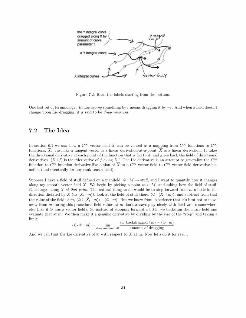
Figure 7.2: Read the labels starting from the bottom.

One last bit of terminology: Backdragging something by t means dragging it by −t. And when a field doesn’tchange upon Lie dragging, it is said to be drag-invariant.

7.2 The Idea

In section 6.1 we saw how a C∞ vector field X can be viewed as a mapping from C∞ functions to C∞

functions, X. Just like a tangent vector is a linear derivation-at-a-point, X is a linear derivation. It takesthe directional derivative at each point of the function that is fed to it, and gives back the field of directionalderivatives. 〈X | f〉 is the “derivative of f along X.” The Lie derivative is an attempt to generalize the C∞

function to C∞ function derivative-like action of X to a C∞ vector field to C∞ vector field derivative-likeaction (and eventually for any rank tensor field).

Suppose I have a field of stuff defined on a manifold, , :M → stuff, and I want to quantify how it changesalong my smooth vector field X. We begin by picking a point m ∈ M , and asking how the field of stuff,,, changes along X at that point. The natural thing to do would be to step forward from m a little in thedirection dictated by X (to 〈Xt | m〉), look at the field of stuff there, 〈, | 〈Xt | m〉〉, and subtract from that

the value of the field at m, 〈, | 〈Xt | m〉〉− 〈, | m〉. But we know from experience that it’s best not to moveaway from m during this procedure; field values at m don’t always play nicely with field values somewhereelse (like if , was a vector field). So instead of stepping forward a little, we backdrag the entire field andevaluate that at m. We then make it a genuine derivative by dividing by the size of the “step” and taking alimit:

〈£X, | m〉 = limdrag amount→0

〈, backdragged | m〉 − 〈, | m〉

amount of dragging

And we call that the Lie derivative of , with respect to X at m. Now let’s do it for real...

34

7.3 The Definition

The Lie derivative of a smooth vector field Y with respect to a smooth vector field X is the vector field £XY

defined as follows.

〈£XY | m〉 = limt→0

〈dX−t ◦ Y ◦ Xt | m〉 − 〈Y | m〉

t

It is the limit of a Tm,M -valued function at each point m. According to the previous section, all we need todo to figure out how to define the Lie derivative of something is figure out how to drag it. For example, let’sapply the same concept to a real-valued function on the manifold, f :M → R. The previous section tells usto define it’s Lie derivative as:

〈£Xf | m〉 = limt→0

〈f ◦ Xt | m〉 − 〈f | m〉

t

Let γm be the integral curve of X that starts at m. Then

〈£Xf | m〉 = limt→0

〈f ◦ γm | t〉 − 〈f ◦ γm | 0〉

t

= 〈(f ◦ γm)′ | 0〉

= 〈〈( ◦ γm)′ | 0〉 | f〉

= 〈〈X ◦ γm | 0〉 | f〉

= 〈〈X | m〉 | f〉

= 〈〈X | f〉 | m〉

So £Xf = 〈X | f〉. This is a pleasant result; it reinforces the notion that the Lie derivative £X generalizesthe action of X on real-valued functions.

7.4 Other Ways of Looking at It

£XY has a pretty simple appearance in a drag-invariant basis. Suppose {Ei} is a drag-invariant basis field.

That is, suppose that for each i we had Ei = dXt ◦ Ei ◦ X−t for all t. (One could obtain such a basis field bystarting out with a set of basis vectors at some point on each integral curve of X, then dragging them aroundto define the rest of the basis field. So if I know 〈Ei | m〉 then I may define 〈Ei | 〈Xt | m〉〉 = 〈dXt | 〈Ei | m〉〉

and this would force Ei to be drag invariant). Now express Y in this basis: Y = Y iEi, where Yi... M → R

are component functions. In the following lines we use the linearity of the differential (which is easy toprove straight from the definition in section 4.1). We also use the fact that (dψ)← = d(ψ←), which is also

35

straight-forward to prove.

〈£XY | m〉 = limt→0

〈dX−t | 〈Y | 〈Xt | m〉〉〉 − 〈Y | m〉

t

= limt→0

〈dX−t | 〈Y i | 〈Xt | m〉〉 · 〈Ei | 〈Xt | m〉〉〉 − 〈Y | m〉

t

= limt→0

〈Y i | 〈Xt | m〉〉 · 〈dX−t | 〈Ei | 〈Xt | m〉〉〉 − 〈Y | m〉

t

= limt→0

〈Y i | 〈Xt | m〉〉 · 〈dX−t | 〈dXt | 〈Ei | m〉〉〉 − 〈Y i | m〉 · 〈Ei | m〉

t

= limt→0

〈Y i | 〈Xt | m〉〉 − 〈Y i | m〉

t· 〈Ei | m〉

= 〈Ei | m〉 limt→0

〈Y i | 〈Xt | m〉〉 − 〈Y i | m〉

t

The limit that appears here is just, by definition, 〈£XYi

| m〉. According to what we previously showed,that’s just 〈〈X | Y i〉 | m〉. So the Lie derivative takes the following simple form in our drag-invariant basisfield:

£XY = 〈X | Y i〉 · Ei

This is yet another way to have defined Lie derivatives. We could have said that the Lie derivative of a vectorfield with respect to X is the derivative of its components along X in a drag-invariant basis field. When weextend our definition this statement will also hold for the components of a tensor field in a drag-invariantbasis field. Another interesting calculation is to examine £∂1Y , the Lie derivative with respect to the firstcoordinate basis field for some coordinate system φ.

Consider the basis field {∂i} for a coordinate system φ with coordinate functions xi. First I claim that∂i is a drag-invariant basis field with respect to ∂1. We showed that dragging a vector field is the samething as taking its integral curves, dragging them, and looking at the vector field associated with the newcurves. This means the drag-invariance of a vector field is equivalent to the drag invariance of the set ofintegral curves. The integral curves of ∂i are easy to solve for in the φ coordinate system. The result is

〈φ ◦ (∂i)t | m〉 = (〈x1 | m〉, 〈x2 | m〉, . . . , 〈xi | m〉+t, . . . , 〈xn | m〉). (Just write down the differential equationsfor the components and the initial condition then solve, as explained in section 6.3). So the flow of ∂i justadds t to the ith coordinate of a point. In particular the flow of ∂1 just adds t to the first coordinate of

a point. Lie dragging a whole integral curve of ∂i, γ 7→ (∂1)t ◦ γ, would then just add t (a constant) tothe first coordinate of the curve, which obviously produces some other integral curve of ∂i. So Lie draggingtakes integral curves of ∂i to integral curves of ∂i, leaving the whole set of integral curves drag-invariant.According to what we said this means that ∂i is drag-invariant with respect to ∂1. Using the results fromthe previous calculation, we may now write the Lie derivative in a simple way:

£∂1Y = 〈∂1 | Y i〉 · ∂i

where 〈∂1 | Y i〉 is of course just the real-valued function ∂Y i◦φ←

∂x1 . We have shown that £∂1 takes the derivativeof all the components of a vector field with respect to the first coordinate! This property of £∂1 will also bevalid for tensor components when we extend our definition. Let’s do that now.

36

7.5 Extending the Definition

Section 7.2 has already laid out the conceptual framework behind defining Lie derivatives. All that remainsis to figure out how to drag any rank tensor field along a vector field. Let’s start with dual vector fields.Recall that we were able to drag a vector (an action on functions) along a diffeomorphism by backdraggingthe functions it acts on. We essentially moved the vector through a diffeomorphism by moving its effect onfunctions. Our dragging tool was thus the differential map, though we don’t really call it dragging unlessthe diffeomorphism comes from the flow of a vector field.

Since a dual vector w is just an action on vectors, we may move the dual vector through a diffeomorphismby moving its effect on vectors, which we now know how to move with the differential. So the dragged dualvector is that map which upon being fed a vector backdrags it and feeds it to the original dual vector. Fora diffeomorphism ψ : M → M and some m ∈ M we define Dψ : T ∗m,M → T ∗

〈ψ | m〉,Msuch that for any dual

vector w ∈ T ∗m,M ,〈〈Dψ | w〉 | v〉 = 〈w | 〈dψ← | v〉〉 for all v ∈ T〈ψ | m〉,M

(Note: Again Dψm,M or Dψm would be better notation, but I’ll mush together all the Dψm’s when I useDψ. Also be warned that authors like to define the inverse of this map instead of what I’ve done, and theycall it δψ. I don’t see the point of this, we would just have to keep taking inverses later on. So that’s whyI’m using capital D instead of δ.)

Now we have the ability to Lie drag dual vectors along vector fields, w 7→ 〈DXt | w〉. And similarly we may

Lie drag dual vector fields, W 7→ DXt ◦W ◦ X−t. We then define the Lie derivative of a dual vector fieldaccording to the same scheme:

〈£XW | m〉 = limt→0

〈DX−t ◦W ◦ Xt | m〉 − 〈W | m〉

t

You’ve probably already figured out how we’re going to Lie drag a tensor along a vector field. Being amultilinear operator on vectors and dual vectors, a tensor may be moved through a diffeomorphism by usingthe diffeomorphism to move its effect on vectors and dual vectors, both of which we now know how to move.For a diffeomorphism ψ :M →M and some m ∈M we define Dr

sψ : T rs (Tm,M ) → T rs (T〈ψ | m〉,M ) such that

for any (r, s) type tensor, T ∈ T rs (Tm,M ) we have:

〈〈Drsψ | T 〉 | (w1, . . . , wr, v1, . . . , vs)〉 = 〈T | (〈Dψ← | w1〉, . . . , 〈Dψ

←| wr〉, 〈dψ

←| v1〉, . . . , 〈dψ

←| vs〉) 〉

for all w1, . . . , wr ∈ T ∗〈ψ | m〉,M

and v1, . . . , vs ∈ T〈ψ | m〉,M

We may now Lie drag (r, s) type tensors, T 7→ 〈DrsXt | T 〉.

And we may Lie drag (r, s) type tensor fields, U 7→ DrsXt ◦ U ◦ X−t.

And we may define the Lie derivative of an (r, s) tensor field U with respect to a smooth vector field X:

〈£XU | m〉 = limt→0

〈DrsX−t ◦ U ◦ Xt | m〉 − 〈U | m〉

t

So £XU is another (r, s) tensor field defined in terms of the limit of a tensor-valued function at each point.Now you are in a good position to go back and verify the properties we claimed would still hold after

37

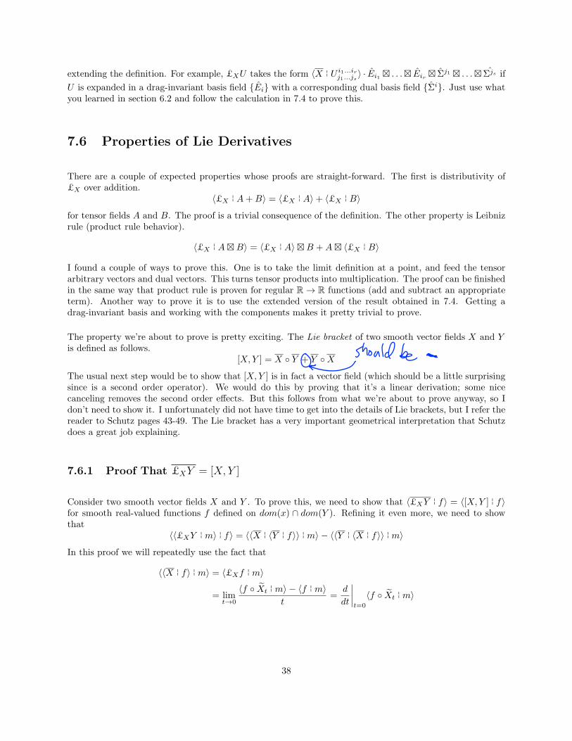
extending the definition. For example, £XU takes the form 〈X | U i1...irj1...js〉 · Ei1 ⊠ . . .⊠ Eir ⊠ Σj1 ⊠ . . .⊠ Σjs if

U is expanded in a drag-invariant basis field {Ei} with a corresponding dual basis field {Σi}. Just use whatyou learned in section 6.2 and follow the calculation in 7.4 to prove this.

7.6 Properties of Lie Derivatives

There are a couple of expected properties whose proofs are straight-forward. The first is distributivity of£X over addition.

〈£X | A+B〉 = 〈£X | A〉+ 〈£X | B〉

for tensor fields A and B. The proof is a trivial consequence of the definition. The other property is Leibnizrule (product rule behavior).

〈£X | A⊠B〉 = 〈£X | A〉⊠B +A⊠ 〈£X | B〉

I found a couple of ways to prove this. One is to take the limit definition at a point, and feed the tensorarbitrary vectors and dual vectors. This turns tensor products into multiplication. The proof can be finishedin the same way that product rule is proven for regular R → R functions (add and subtract an appropriateterm). Another way to prove it is to use the extended version of the result obtained in 7.4. Getting adrag-invariant basis and working with the components makes it pretty trivial to prove.

The property we’re about to prove is pretty exciting. The Lie bracket of two smooth vector fields X and Yis defined as follows.

[X,Y ] = X ◦ Y + Y ◦X

The usual next step would be to show that [X,Y ] is in fact a vector field (which should be a little surprisingsince is a second order operator). We would do this by proving that it’s a linear derivation; some nicecanceling removes the second order effects. But this follows from what we’re about to prove anyway, so Idon’t need to show it. I unfortunately did not have time to get into the details of Lie brackets, but I refer thereader to Schutz pages 43-49. The Lie bracket has a very important geometrical interpretation that Schutzdoes a great job explaining.

7.6.1 Proof That £XY = [X, Y ]

Consider two smooth vector fields X and Y . To prove this, we need to show that 〈£XY | f〉 = 〈[X,Y ] | f〉for smooth real-valued functions f defined on dom(x) ∩ dom(Y ). Refining it even more, we need to showthat

〈〈£XY | m〉 | f〉 = 〈〈X | 〈Y | f〉〉 | m〉 − 〈〈Y | 〈X | f〉〉 | m〉

In this proof we will repeatedly use the fact that

〈〈X | f〉 | m〉 = 〈£Xf | m〉

= limt→0

〈f ◦ Xt | m〉 − 〈f | m〉

t=

d

dt

∣∣∣∣t=0

〈f ◦ Xt | m〉

38

for any smooth vector field and scalar field X and f . We already showed this in section 7.3. We’ll start byrewriting what we need to show, then we’ll work on the left side of the equal sign.

〈〈X | 〈Y | f〉〉 | m〉 − 〈〈Y | 〈X | f〉〉 | m〉 =d

dt

∣∣∣∣t=0

〈〈Y | f〉 | 〈Xt | m〉〉 −d

du

∣∣∣∣u=0

〈〈X | f〉 | 〈Yu | m〉〉

=d

dt

∣∣∣∣t=0

d

du

∣∣∣∣u=0

〈f ◦ Yu ◦ Xt | m〉 −d

du

∣∣∣∣u=0

d

ds

∣∣∣∣s=0

〈f ◦ Xs ◦ Yu | m〉

=∂2

∂t∂u

∣∣∣∣(t,u)=(0,0)

〈f ◦ Yu ◦ Xt | m〉 −∂2

∂s∂u

∣∣∣∣(u,s)=(0,0)

〈f ◦ Xs ◦ Yu | m〉

We used the smoothness of our maps to switch the order of the partial derivatives in the last step. Of coursethe choices of letters for parameters like t, u, s were arbitrary. The notation “ d

dt” is informal anyway. I just

chose letters that will match the result we get at the end. What we must show has been reduced to:

〈〈£XY | m〉 | f〉 =∂2

∂t∂u

∣∣∣∣(t,u)=(0,0)

〈f ◦ Yu ◦ Xt | m〉 −∂2

∂s∂u

∣∣∣∣(u,s)=(0,0)

〈f ◦ Xs ◦ Yu | m〉

Let’s get to work on the left hand side.

〈〈£XY | m〉 | f〉 =

⟨limt→0

〈dX−t ◦ Y ◦ Xt | m〉 − 〈Y | m〉

t| f

⟩

= limt→0

〈〈dX−t ◦ Y ◦ Xt | m〉 | f〉 − 〈〈Y | m〉 | f〉

t

= limt→0

〈〈Y | 〈Xt | m〉〉 | f ◦ X−t〉 − 〈〈Y | m〉 | f〉

t

= limt→0

〈〈Y | f ◦ X−t〉 | 〈Xt | m〉〉 − 〈〈Y | f〉 | m〉

t

=d

dt

∣∣∣∣t=0

〈〈Y | f ◦ X−t〉 | 〈Xt | m〉〉

=d

dt

∣∣∣∣t=0

d

du

∣∣∣∣u=0

〈f ◦ X−t ◦ Yu | 〈Xt | m〉〉

=∂2

∂t∂u

∣∣∣∣(t,u)=(0,0)

〈f ◦ X−t ◦ Yu ◦ Xt | m〉

Here’s the tricky bit. We’re going to define a couple of functions so we can formalize away from the “ ddt”

notation. This will help us to use the chain rule correctly. Define a function κ... R3 → R as follows.

〈κ | (t, u, s)〉 = 〈f ◦ Xs ◦ Yu ◦ Xt | m〉

39

So the thing being differentiated above is the mapping (t, u) 7→ 〈κ | (t, u,−t)〉. Notice that κ is well-definedon some neighborhood of (0, 0, 0). Define j : R2 → R

3 to be the mapping (t, u) 7→ (t, u,−t) with componentfunctions 〈j1 | (t, u)〉 = t, 〈j2 | (t, u)〉 = u, and 〈j3 | (t, u)〉 = −t. Now the thing being differentiated above isκ ◦ j. Let number subscripts denote partial derivatives. Then we have

〈〈£XY | m〉 | f〉 = 〈(κ ◦ j)21 | (0, 0)〉

Using chain rule (m© is matrix multiplication):

(κ ◦ j)′ =[(κ ◦ j)1 (κ ◦ j)2

]

=[κ1 ◦ j κ2 ◦ j κ3 ◦ j

]m©

j11 j21

j12 j22

j13 j23

=[κ1 ◦ j κ2 ◦ j κ3 ◦ j

]m©

1 0

0 1

−1 0

So the first derivative gives

(κ ◦ j)2 =[κ1 ◦ j κ2 ◦ j κ3 ◦ j

]m©

010

= κ2 ◦ j

And similarly the next derivative gives

(κ ◦ j)21 = (κ2 ◦ j)1 =[κ21 ◦ j κ22 ◦ j κ23 ◦ j

]m©

10−1

= κ21 ◦ j − κ23 ◦ j

And now we may switch back to the less formal notation:

〈〈£XY | m〉 | f〉 = 〈κ21 ◦ j − κ23 ◦ j | (0, 0)〉

= 〈κ21 − κ23 | (0, 0, 0)〉

=∂2

∂t∂u

∣∣∣∣(t,u,s)=(0,0,0)

〈f ◦ Xs ◦ Yu ◦ Xt | m〉 −∂2

∂s∂u

∣∣∣∣(t,u,s)=(0,0,0)

〈f ◦ Xs ◦ Yu ◦ Xt | m〉

=∂2

∂t∂u

∣∣∣∣(t,u)=(0,0)

〈f ◦ Yu ◦ Xt | m〉 −∂2

∂s∂u

∣∣∣∣(u,s)=(0,0)

〈f ◦ Xs ◦ Yu | m〉

= 〈〈[X,Y ] | f〉 | m〉

Thus £XY = [X,Y ] and the proof is done.

40

Chapter 8

Appendix

8.1 Notation

I describe the notation I use within the text where I first use it. However I’m providing a list here in caseyou want to skip around the paper.

• Fm,M is the set of real-valued functions smoothly defined on a neighborhood of a point m on themanifold M .

• Tm,M is the tangent space at the point m in the manifold M .

• V ∗ is the dual space to the vector space V .

• T rs V is the vector space of (r, s) type tensors over the vector space V .

• dom(f) and ran(f) are the domain and range of a function f .

• φ∂i is the ith coordinate basis field that comes from the coordinate system φ. Sometimes I leave outthe φ.

• f... A→ B is just like f : A→ B except the domain of f is some subset of A.

• Be careful of the differential (like dxi or dXt), they tend to have meanings that change in subtle ways.Their particular usage is described in the text each time.

• X is the C∞ function to function way of looking at a vector field X. Most people just use X to referto both.

• X is the flow of the smooth vector field X. When I say flow I mean the one-parameter group associatedwith the vector field.

• 〈f | x〉 is an alternative (and better) notation for f(x), evaluating a function at a point. Since it’sunconventional I avoided it as much as I could, but I was forced to use it at the end.

• The underscore notation is sometimes used to denote a function. For example the parabola defined byf(x) = x2 is just f = 2. And the tangent vector defined by t(f) = (f ◦ γ)′ is t = ( ◦ γ)′

41