Embed Size (px)
Citation preview

arX
iv:h
ep-t
h/96
1211
4v1
11
Dec
199
6
FERMILAB-PUB-96/445-T
INTRODUCTION TO SUPERSYMMETRY
JOSEPH D. LYKKEN
Fermi National Accelerator Laboratory
P.O. Box 500
Batavia, IL 60510
These lectures give a self-contained introduction to supersymmetry from a modernperspective. Emphasis is placed on material essential to understanding duality.Topics include: central charges and BPS-saturated states, supersymmetric nonlin-ear sigma models, N=2 Yang-Mills theory, holomorphy and the N=2 Yang-Mills β
function, supersymmetry in 2, 6, 10, and 11 spacetime dimensions.
1 Introduction
“Never mind, lads. Same time tomorrow. We must get a winner
one day.”
– Peter Cook, as the doomsday prophet in “The End of the World”.
Supersymmetry, along with its monozygotic sibling superstring theory, hasbecome the dominant framework for formulating physics beyond the standardmodel. This despite the fact that, as of this morning, there is no unambiguousexperimental evidence for either idea. Theorists find supersymmetry appealingfor reasons which are both phenomenological and technical. In these lectures Iwill focus exclusively on the technical appeal. There are many good recent re-views of the phenomenology of supersymmetry. 1 Some good technical reviewsare Wess and Bagger, 2 West, 3 and Sohnius. 4
The goal of these lectures is to provide the student with the technical back-ground requisite for the recent applications of duality ideas to supersymmetricgauge theories and superstrings. More specifically, if you absorb the materialin these lectures, you will understand Section 2 of Seiberg and Witten, 5 andyou will have a vague notion of why there might be such a thing as M -theory.Beyond that, you’re on your own.
2 Representations of Supersymmetry
2.1 The general 4-dimensional supersymmetry algebra
A symmetry of the S-matrix means that the symmetry transformations havethe effect of merely reshuffling the asymptotic single and multiparticle states.The known symmetries of the S-matrix in particle physics are:
1

• Poincare invariance, the semi-direct product of translations and Lorentzrotations, with generators Pm, Mmn.
• So-called “internal” global symmetries, related to conserved quantumnumbers such as electric charge and isospin. The symmetry generatorsare Lorentz scalars and generate a Lie algebra,
[Bℓ, Bk] = iCjℓkBj , (1)
where the Cjℓk are structure constants.
• Discrete symmetries: C, P, and T.
In 1967, Coleman and Mandula 6 provided a rigorous argument whichproves that, given certain assumptions, the above are the only possible sym-metries of the S-matrix. The reader is encouraged to study this classic paperand think about the physical and technical assumptions which are made there.
The Coleman-Mandula theorem can be evaded by weakening one or moreof its assumptions. In particular, the theorem assumes that the symmetry alge-bra of the S-matrix involves only commutators. Weakening this assumption toallow anticommuting generators as well as commuting generators leads to thepossibility of supersymmetry. Supersymmetry (or SUSY for short) is definedas the introduction of anticommuting symmetry generators which transform inthe (1
2 , 0) and (0, 12 ) (i.e. spinor) representations of the Lorentz group. Since
these new symmetry generators are spinors, not scalars, supersymmetry is notan internal symmetry. It is rather an extension of the Poincare spacetimesymmetries. Supersymmetry, defined as the extension of the Poincare symme-try algebra by anticommuting spinor generators, has an obvious extension tospacetime dimensions other than four; the Coleman-Mandula theorem, on theother hand, has no obvious extension beyond four dimensions.
In 1975, Haag, Lopuszanski, and Sohnius 7 proved that supersymmetryis the only additional symmetry of the S-matrix allowed by this weaker setof assumptions. Of course, one could imagine that a further weakening ofassumptions might lead to more new symmetries, but to date no physicallycompelling examples have been exhibited. 8 This is the basis of the strong butnot unreasonable assertion that:
Supersymmetry is the only possible extension of the known
spacetime symmetries of particle physics.
In four-dimensional Weyl spinor notation (see the Appendix) the N super-symmetry generators are denoted by QA
α , A=1, . . .N. The most general four-
2

dimensional supersymmetry algebra is given in the Appendix; here we will becontent with checking some of the features of this algebra.
The anticommutator of the QAα with their adjoints is:
QAα , QβB = 2σm
αβPmδ
AB . (2)
To see this, note the right-hand side of Eq. 2 must transform as (12 ,
12 ) under
the Lorentz group. The most general such object that can be constructed outof Pm, Mmn, and Bℓ has the form:
σmαβPmC
AB ,
where the CAB are complex Lorentz scalar coefficients. Taking the adjoint of
the left-hand side of Eq. 2, using
(
σmαβ
)†
= σmβα ,
(
QAα
)†= Q
A
α , (3)
tells us that CAB is a hermitian matrix. Furthermore, since Q,Q is a positive
definite operator, CAB is a positive definite hermitian matrix. This means that
we can always choose a basis for the QAα such that CA
B is proportional to δAB.
The factor of two in Eq. 2 is simply a convention.The SUSY generators QA
α commute with the translation generators:
[QAα , Pm] = [Q
A
α , Pm] = 0 . (4)
This is not obvious since the most general form consistent with Lorentz invari-ance is:
[
QAα , Pm
]
= ZABσαβmQ
βB
[QαA, Pm] =
(
ZAB
)∗QB
β σαβm , (5)
where the ZAB are complex Lorentz scalar coefficients. Note we have invoked
here the Haag, Lopuszanski, Sohnius theorem which tells us that there are no(12 , 1) or (1, 1
2 ) symmetry generators.To see that the ZA
B all vanish, the first step is to plug Eq. 5 into the Jacobiidentity:
[
[QAα , Pm], Pn
]
+ (cyclic) = 0 . (6)
Using Eq. 240 this yields:
− 4i (ZZ∗)AB σ
βmnαQ
Bβ = 0 , (7)
3

which implies that the matrix ZZ∗ vanishes.This is not enough to conclude that ZA
B itself vanishes, but we can getmore information by considering the most general form of the anticommutatorof two Q’s:
QAα , Q
Bβ = ǫαβX
AB + ǫβγσmnγα MmnY
AB . (8)
Here we have used the fact that the rhs must transform as (0, 0) + (1, 0) un-der the Lorentz group. The spinor structure of the two terms on the rhs isantisymmetric/symmetric respectively under α ↔ β, so the complex Lorentzscalar matrices XAB and Y AB are also antisymmetric/symmetric respectively.
Now we consider ǫαβ contracted on the Jacobi identity[
QAα , Q
Bβ , Pm
]
+
[Pm, QAα ], QB
β
−
[QBβ , Pm], QA
α
= 0 . (9)
Since XAB commutes with Pm, and plugging in Eqs. 2,5,232 and 233, theabove reduces to
− 4(
ZAB − ZBA)
Pm = 0 , (10)
and thus ZAB is symmetric. Combined with ZZ∗=0 this means that ZZ†=0,
which implies that ZAB vanishes, giving Eq. 4.
Having established Eq. 4, the symmetric part of the Jacobi identity Eq. 9implies that MmnY
AB commutes with Pm, which can only be true if Y AB
vanishes. Thus:QA
α , QBβ = ǫαβX
AB . (11)
The complex Lorentz scalars XAB are called central charges; furthermanipulations with the Jacobi identities show that the XAB commute withthe QA
α , QαA, and in fact generate an Abelian invariant subalgebra of thecompact Lie algebra generated by Bℓ. Thus we can write:
XAB = aℓAB Bℓ , (12)
where the complex coefficients aℓAB obey the intertwining relation Eq. 264.
2.2 The 4-dimensional N=1 supersymmetry algebra
The Appendix also contains the special case of the four-dimensional N=1 su-persymmetry algebra. For N=1 the central chargesXAB vanish by antisymme-try, and the coefficients Sℓ are real. The Jacobi identity for [[Q,B], B] impliesthat the structure constants Ck
mℓ vanish, so the internal symmetry algebra isAbelian. Starting with
[Qα, Bℓ] = SℓQα
[Qα, Bℓ] = −SℓQα , (13)
4

it is clear that we can rescale the Abelian generators Bℓ and write:
[Qα, Bℓ] = Qα
[Qα, Bℓ] = −Qα . (14)
Clearly only one independent combination of the Abelian generators actuallyhas a nonzero commutator with Qα and Qα; let us denote this U(1) generatorby R:
[Qα, R] = Qα
[Qα, R] = −Qα . (15)
Thus the N=1 SUSY algebra in general possesses an internal (global) U(1)symmetry known as R symmetry. Note that the SUSY generators haveR-charge +1 and -1, respectively.
2.3 SUSY Casimirs
Since we wish to characterize the irreducible representations of supersymmetryon asymptotic single particle states, we need to exhibit the Casimir operators.It suffices to do this for the N=1 SUSY algebra, as the extension to N>1 isstraightforward.
Recall that the Poincare algebra has two Casimirs: the mass operatorP 2 = PmP
m, with eigenvalues m2, and the square of the Pauli-Ljubanskivector
Wm =1
2ǫmnpqP
nMpq . (16)
W 2 has eigenvalues −m2s(s+ 1), s=0, 12 , 1, . . . for massive states, and Wm =
λPm for massless states, where λ is the helicity.For N=1 SUSY, P 2 is still a Casimir (since P commutes with Q and Q),
but W 2 is not (M does not commute with Q and Q). The actual Casimirs areP 2 and C2, where
C2 = CmnCmn ,
Cmn = BmPn −BnPm , (17)
Bm = Wm − 1
4Qασ
αβm Qβ .
This is easily verified using the commutators:
[Wm, Qα] = −iσβmnαQβP
n ,
[Qβ σβγm Qγ , Qα] = −2PmQα + 4iσβ
nmαPnQβ , (18)
5

which imply:
[Cmn, Qα] = [Bm, Qα]Pn − [Bn, Qα]Pm
= 0 . (19)
2.4 Classification of SUSY irreps on single particle states
We now have enough machinery to construct all possible irreducible represen-tations of supersymmetry on asymptotic (on-shell) physical states. We beginwith N=1 SUSY, treating the massive and massless states separately. Unlikethe case of Poincare symmetry, we do not have to consider tachyons – they areforbidden by the fact that Q,Q is positive definite.
N=1 SUSY, massive states
We analyze massive states from the rest frame Pm = (m,~0). We can write:
C2 = 2m4JiJi ,
Ji ≡ Si −1
4mQσiQ , (20)
where Si is the spin operator and i is a spatial index: i = 1, 2, 3. Both Si andσαβ
i obey the SU(2) algebra, so
[Ji, Jj ] = iǫijkJk , (21)
and J2 has eigenvalues j(j + 1), j equal integers or half-integers.
The commutator of Ji with either Q or Q is proportional to ~P and thusvanishes since we are in the rest frame. Qα, Qα are in fact two pairs ofcreation/annihilation operators which fill out the N=1 massive SUSY irrep offixed m and j:
Qα, Qβ = 2mσ0αβ
= 2m
(
1 00 1
)
. (22)
Given any state of definite |m, j〉 we can define a new state
|Ω〉 = Q1Q2 |m, j〉 , (23)
Q1 |Ω〉 = Q2 |Ω〉 = 0 .
Thus |Ω〉 is a Clifford vacuum state with respect to the fermionic annihilationoperators Q1, Q2. Note that |Ω〉 has degeneracy 2j+1 since j3 takes values−j, . . . j.
6

Acting on |Ω〉, Ji reduces to just the spin operator Si, so |Ω〉 is actuallyan eigenstate of spin:
|Ω〉 = |m, s, s3〉 . (24)
Thus we can characterize all the states in the SUSY irrep by mass and spin.It is convenient to define conventionally normalized creation/annihilation
operators:
a1,2 =1√2m
Q1,2 ,
a†1,2 =1√2m
Q1,2 . (25)
Then for a given |Ω〉 the full massive SUSY irrep is:
|Ω〉a†1 |Ω〉 (26)
a†2 |Ω〉1√2a†1a
†2 |Ω〉 = − 1√
2a†2a
†1 |Ω〉
There are a total of 4(2j+1) states in the massive irrep.We compute the spin of these states by using the commutators:
[
S3,
(
a†2a†1
)
]
=1
2
(
a†2−a†1
)
. (27)
Thus for |Ω〉 = |m, j, j3〉 we get states of spin s3 = j3, j3− 12 , j3+ 1
2 , j3.As an example, consider the j=0 or fundamental N=1 massive irrep.
Since |Ω〉 has spin zero there are a total of four states in the irrep, with spinss3 = 0, − 1
2 , 12 , and 0, respectively. Since the parity operation interchanges
a†1 with a†2, one of the spin zero states is a pseudoscalar. Thus these fourstates correspond to one massive Weyl fermion, one real scalar, and one realpseudoscalar.
N=1 SUSY, massless states
We analyze massless states from the light-like reference frame Pm = (E, 0, 0, E).In this case
C2 = −2E2(B0 −B3)2 = − 1
2E2Q2Q2Q2Q2 = 0 . (28)
7

Also we have:
Q1, Q1 = 4E ,
Q2, Q2 = 0 . (29)
We can define a vacuum state |Ω〉 as in the massive case. However we noticefrom Eq. 29 that the creation operator Q2 makes states of zero norm:
〈Ω|Q2Q2 |Ω〉 = 0 . (30)
This means that we can set Q2 equal to zero in the operator sense. Effectivelythere is just one pair of creation/annihilation operators:
a =1
2√EQ1 , a† =
1
2√EQ1 . (31)
|Ω〉 is nondegenerate and has definite helicity λ. The creation operator a†
transforms like (0, 12 ) under the Lorentz group, thus it increases helicity by
1/2. The massless N=1 SUSY irreps each contain two states:
|Ω〉 helicity λ ,
a† |Ω〉 helicity λ+1
2. (32)
However this is not a CPT eigenstate in general, requiring that we pair twomassless SUSY irreps to obtain four states with helicities λ, λ+ 1
2 , −λ− 12 , and
−λ.
N>1 SUSY, no central charges, massless states
Here we have N creation operators a†A. These generate a total of 2N states inthe SUSY irrep. The states have the form:
1√n!a†A1
. . . a†An|Ω〉 , (33)
with degeneracy given by the binomial coefficient(
Nn
)
. Denoting the helicity
of |Ω〉 by λ, the helicities in the irrep are λ, λ+ 12 , . . .λ+N
2 . This is not a CPTeigenstate except in the special case λ = −N/4. Examples of some of the moreimportant irreps are given in Table 1.
8
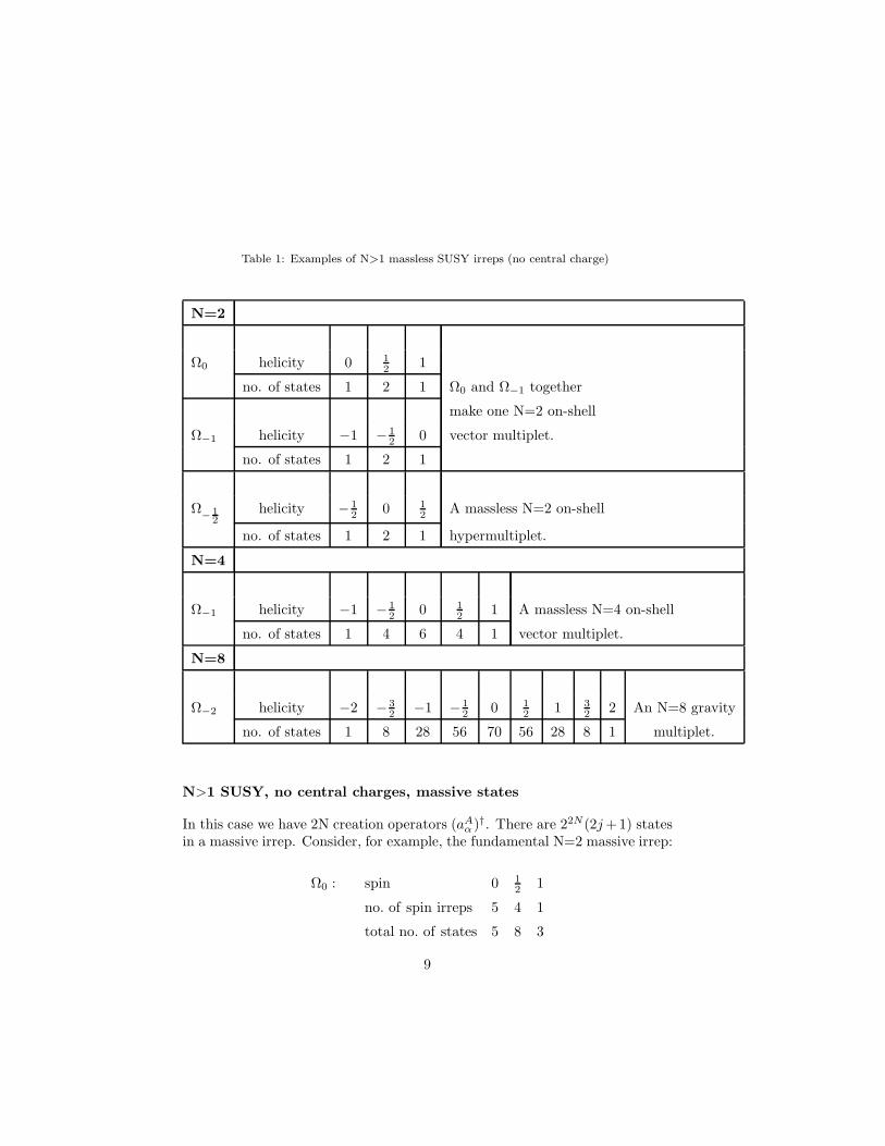
Table 1: Examples of N>1 massless SUSY irreps (no central charge)
N=2
Ω0 helicity 0 12 1
no. of states 1 2 1 Ω0 and Ω−1 together
make one N=2 on-shell
Ω−1 helicity −1 − 12 0 vector multiplet.
no. of states 1 2 1
Ω− 1
2helicity − 1
2 0 12 A massless N=2 on-shell
no. of states 1 2 1 hypermultiplet.
N=4
Ω−1 helicity −1 − 12 0 1
2 1 A massless N=4 on-shell
no. of states 1 4 6 4 1 vector multiplet.
N=8
Ω−2 helicity −2 − 32 −1 − 1
2 0 12 1 3
2 2 An N=8 gravity
no. of states 1 8 28 56 70 56 28 8 1 multiplet.
N>1 SUSY, no central charges, massive states
In this case we have 2N creation operators (aAα )†. There are 22N(2j+ 1) states
in a massive irrep. Consider, for example, the fundamental N=2 massive irrep:
Ω0 : spin 0 12 1
no. of spin irreps 5 4 1
total no. of states 5 8 3
9
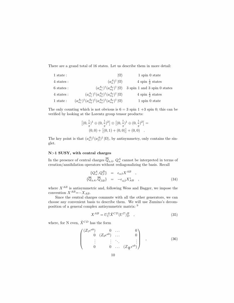
There are a grand total of 16 states. Let us describe them in more detail:
1 state : |Ω〉 1 spin 0 state
4 states : (aAα )† |Ω〉 4 spin 1
2 states
6 states : (aA1
α1)†(aA2
α2)† |Ω〉 3 spin 1 and 3 spin 0 states
4 states : (aA1
α1)†(aA2
α2)†(aA3
α3)† |Ω〉 4 spin 1
2 states
1 state : (aA1
α1)†(aA2
α2)†(aA3
α3)†(aA4
α4)† |Ω〉 1 spin 0 state
The only counting which is not obvious is 6 = 3 spin 1 +3 spin 0; this can beverified by looking at the Lorentz group tensor products:
[
(0,1
2)1 ⊕ (0,
1
2)2]
⊗[
(0,1
2)1 ⊕ (0,
1
2)2]
=
(0, 0) +[
(0, 1) + (0, 0)]
+ (0, 0) .
The key point is that (aAα )†(aA
β )† |Ω〉, by antisymmetry, only contains the sin-glet.
N>1 SUSY, with central charges
In the presence of central charges QαA, QAα cannot be interpreted in terms of
creation/annihilation operators without rediagonalizing the basis. Recall
QAα , Q
Bβ = ǫαβX
AB ,
QαA, QβB = −ǫαβX∗AB , (34)
where XAB is antisymmetric and, following Wess and Bagger, we impose theconvention XAB=−XAB.
Since the central charges commute with all the other generators, we canchoose any convenient basis to describe them. We will use Zumino’s decom-position of a general complex antisymmetric matrix: 9
XAB = UAC X
CD(UT )BD , (35)
where, for N even, XCD has the form
(Z1ǫab) 0 . . . 0
0 (Z2ǫab) . . . 0
......
. . ....
0 0 . . . (ZN
2
ǫab)
, (36)
10

where ǫab=iσ2. For N odd, there is an extra right-hand column of zeroes andbottom row of zeroes. In this decomposition the “eigenvalues” Z1, Z2, . . . Z[ N
2 ]are real and nonnegative.
Consider now the massive states in the rest frame. In the basis defined byZumino’s decomposition we have:
Qα, Qβ = 2mσ0αβδab δ
LM ,
QaLα , QbM
β = ǫαβǫabδLMZM , (37)
QαaL, QβbM = −ǫαβǫabδLMZM ,
where the internal indices A, B have now been replaced by the index pairs(a, L), (b,M), with a, b = 1, 2 and L,M = 1, 2, . . . [N
2 ]. Here and in thefollowing, the repeated M index is not summed over.
It is now apparent that there are 2N pairs of creation/annihilation opera-tors:
aLα =
1√2
[
Q1Lα + ǫαβQγ2Lσ
0γβ]
,
(aLα)† =
1√2
[
Qα1L + ǫαβ σ0βγQ2L
γ
]
,
bLα =1√2
[
Q1Lα − ǫαβQγ2Lσ
0γβ]
, (38)
(bLα)† =1√2
[
Qα1L − ǫαβ σ0βγQ2L
γ
]
.
The Lorentz index structure here looks a little strange, but the important pointis that Qα transforms the same as Qα under spatial rotations. Thus (aL
α)†,(bLα)† create states of definite spin.
The anticommutation relation are:
aLα, (a
Mβ )† = (2m+ ZM )σ0
αβδLM ,
bLα, (bMβ )† = (2m− ZM )σ0αβδLM . (39)
This is easily verified from Eqs 37, 38 using the relations:
ǫαδσ0γδǫγβ = −σ0
αβ,
ǫβδσ0δγǫαγ = σ0
αβ. (40)
11

BPS-saturated states
Since a, a† and b, b† are positive definite operators, and since the ZM arenonnegative, we deduce the following:
• For all ZM in any SUSY irrep:
ZM ≤ 2m . (41)
• When ZM < 2m the multiplicities of the massive irreps are the same asfor the case of no central charges.
• The special case is when we saturate the bound, i.e. ZM = 2m for someor all ZM . If e.g. all the ZM saturate the bound, then all of the (bLα)†
are projections onto zero norm states; thus effectively we lose half of thecreation operators. This implies that this massive SUSY irrep has only2N(2j+1) states instead of 22N (2j+1) states.
These reduced multiplicity massive multiplets are often called short mul-
tiplets. The states are often referred to as BPS-saturated states, becauseof the connection to BPS monopoles in supersymmetric gauge theories. 10
For example, let us compare the fundamental N=2 massive irreps. ForN=2 there is only one central charge, Z. For Z < 2m we have the long
multiplet already discussed:
Ωlong0 : spin 0 1
2 1
no. of spin irreps 5 4 1
total no. of states 5 8 3
There are a grand total of 16 states.
For Z = 2m we have BPS-saturated states in a short multiplet:
Ωshort0 : spin 0 1
2 1
no. of spin irreps 2 1 0
total no. of states 2 2 0
There are a grand total of 4 states. Note that the spins and number of statesof this BPS-saturated massive multiplet match those of the N=2 massless
hypermultiplet in Table 1.
12

Let us also compare the j= 12 N=2 massive irreps. For Z < 2m we have a
long multiplet with 32 states:
Ωlong12
: spin 0 12 1 3
2
no. of spin irreps 4 6 4 1
total no. of states 4 12 12 4
For Z = 2m we have a short multiplet with 8 states:
Ωshort12
: spin 0 12 1 3
2
no. of spin irreps 1 2 1 0
total no. of states 1 4 3 0
Note that the spins and number of states of this BPS-saturated massive mul-tiplet match those of the N=2 massless vector multiplet (allowing for the factthat a massless vector eats a scalar in becoming massive).
Automorphisms of the supersymmetry algebra
In the absence of central charges, the general 4-dimensional SUSY algebra hasan obvious U(N) automorphism symmetry:
QAα → UA
BQBα , QαA → QαBU
†BA , (42)
where UAB is a unitary matrix. SUSY irreps on asymptotic single particle
states will automatically carry a representation of the automorphism group.For massless irreps U(N) is the largest automorphism symmetry which respectshelicity.
For massive irreps, we have already noted that Qα and Qα transform thesame way under spatial rotations. Assembling these into a 2N componentobject, one finds that the largest automorphism group which respects spinis USp(2N), the unitary symplectic group of rank N. 11 In the presence ofcentral charges, the automorphism group is still USp(2N) provided that noneof the central charges saturates the BPS bound; this follows from our ability tomake the basis change Eqs. 38, 39. When one central charge saturates the BPSbound, the automorphism group is reduced to USp(N) for N even, USp(N+1)for N odd.
The automorphism symmetries give us constraints on the internal sym-metry group generated by the Bℓ. In the case of no central charges U(N) is
13

the largest possible internal symmetry group which can act nontrivially on theQ’s. With a single central charge, the intertwining relation Eq. 264 impliesthat USp(N) is the largest such group.
Supersymmetry represented on quantum fields
So far we have only discussed representations of SUSY on asymptotic states,not on quantum fields. Qα, Qα can be represented as superspace differentialoperators acting on fields. The Clifford vacuum condition Eq. 23 becomes acommutation condition:
[Qα,Ω(x)] = 0 . (43)
For on-shell fields, the construction of SUSY irreps proceeds as before,with the following exception. If Ω(x) is a real scalar field, then the adjoint ofEq. 43 is
[Qα,Ω(x)] = 0 . (44)
In that case, Eqs. 43, 44 together with the Jacobi identity for [Ω(x), Q], Qimplies that Ω(x) is a constant.
Thus we conclude that Ω(x) must be a complex scalar field. This hasthe effect that some SUSY on-shell irreps on fields have twice as many fieldcomponents as the corresponding irreps for on-shell states. Because we alreadypaired up most SUSY irreps on states to get CPT eigenstates, this doublingreally only effects the SUSY irreps based on the special case Ωλ, λ = −N/4.The first example is the massless N=2 hypermultiplet. On asymptotic singleparticle states this irrep consists of 4 states (see Table 1); the massless N=2hypermultiplet on fields, however, has 8 real components.
2.5 N=1 rigid superspace
Relativistic quantum field theory relies upon the fact that the spacetime coor-dinates xm parametrize the coset space defined as the Poincare group moddedout by the Lorentz group. Clearly it is desirable to find a similar coordinati-zation for supersymmetric field theory. For simplicity we will discuss the caseof N=1 SUSY, deferring N>1 SUSY until Section 5.
The first step is to rewrite the N=1 SUSY algebra as a Lie algebra. Thisrequires that we introduce constant Grassmann spinors θα, θα:
θα, θβ = θα, θβ = θα, θβ = 0 . (45)
This allows us to replace the anticommutators in the N=1 SUSY algebra withcommutators:
[ θ Q, θQ ] = 2θσmθPm ,
14

[ θ Q, θQ ] = 0 , (46)
[ θ Q, θ Q ] = 0 .
Note we have now begun to employ the spinor summation convention discussedin the Appendix.
Given a Lie algebra we can exponentiate to get the general group element:
G(x, θ, θ, ω) = ei[−xmPm+θ Q+θ Q]e−i
2ωmnMmn , (47)
where the minus sign in front of xm is a convention. Note that this form ofthe general N=1 superPoincare group element is unitary since (θQ)†=θQ.
From Eq. 47 it is clear that (xm, θα, θα) parametrizes a 4+4 dimensionalcoset space: N=1 superPoincare mod Lorentz. This coset space is more com-monly known as N=1 rigid superspace; “rigid” refers to the fact that weare discussing global supersymmetry.
There are great advantages to constructing supersymmetric field theoriesin the superspace/superfield formalism, just as there are great advantages toconstructing relativistic quantum field theories in a manifestly Lorentz covari-ant formalism. Our rather long technical detour into superspace and superfieldconstructions will pay off nicely when we begin the construction of supersym-metric actions.
Superspace derivatives
Here we collect the basic notation and properties of N=1 superspace deriva-tives.
∂α =∂
∂θα, ∂α =
∂
∂θα= −ǫαβ∂β ,
∂α
=∂
∂θα
, ∂α =∂
∂θα
= −ǫαβ∂β
,
∂αθβ = δβ
α , ∂αθβ = δα
β,
∂αθβ = −ǫαβ , ∂αθβ = −ǫαβ , (48)
∂αθ
β= −ǫαβ , ∂αθβ = −ǫαβ ,
∂αθβθγ = δβ
αθγ − δγ
αθβ ,
∂α(θθ) = 2θα , ∂α(θθ) = −2θα ,
∂2(θθ) = 4 , ∂2(θθ) = 4 .
15

Superspace integration
We begin with the Berezin integral for a single Grassmann parameter θ:∫
dθ θ = 1 ,
∫
dθ = 0 , (49)
∫
dθ f(θ) = f1 ,
where we have used the fact that an arbitrary function of a single Grassmannparameter θ has the Taylor series expansion f(θ) = f0 + θf1.
We note three facts which follow from the definitions of Eq. 49.
• Berezin integration is translationally invariant:∫
d(θ + ξ) f(θ + ξ) =
∫
dθ f(θ) ,
∫
dθd
dθf(θ) = 0 . (50)
• Berezin integration is equivalent to differentiation:
d
dθf(θ) = f1 =
∫
dθ f(θ) . (51)
• We can define a Grassmann delta function by
δ(θ) ≡ θ . (52)
These results are easily generalized to the case of the N=1 superspacecoordinates θα, θα. The important notational conventions are:
d2θ = − 1
4dθα dθβ ǫαβ ,
d2θ = − 1
4dθα dθβ ǫ
αβ , (53)
d4θ = d2θ d2θ .
Using this notation and the spinor summation convention, we have the follow-ing identities:
∫
d2θ θ θ = 1 ,
∫
d2θ θ θ = 1 . (54)
16

Superspace covariant derivatives
If we wanted to treat a general curved N=1 superspace, we would have tointroduce a 4+4=8-dimensional vielbein and spin connection. Using M todenote an 8-dimensional superspace index, and A to denote an 8-dimensionalsuper-tangent space index, we can write the vielbein and spin connection asEA
M and WmnA respectively. The general form of a covariant derivative in such
a space is thus
DM = EAM (∂A +
1
2Wmn
A Mmn) , (55)
where ∂A=(∂m, ∂α, ∂α).Naively one might expect thatDM reduces to ∂M for N=1 rigid superspace,
since the rigid superspace has zero curvature. However it is possible to show 3
that N=1 rigid superspace has nonzero torsion, and thus that the vielbein isnontrivial. The covariant derivatives for N=1 rigid superspace are given by:
Dm = ∂m ,
Dα = ∂α + iσmαβθ
β∂m ,
Dα = −∂α − iθβσmβα∂m , (56)
Dα = −∂α − iθβσmβα∂m ,
Dα
= ∂α
+ iσmαβθβ∂m .
3 N=1 Superfields
3.1 The general N=1 scalar superfield
The general scalar superfield Φ(x, θ, θ) is just a scalar function in N=1 rigidsuperspace. It has a finite Taylor expansion in powers of θα, θα; this is knownas the component expansion of the superfield:
Φ(x, θ, θ) = f(x) + θφ(x) + θχ(x) + θθm(x) + θθn(x)
+θσmθvm(x) + (θθ)θλ(x) + (θθ)θψ(x) + (θθ)(θθ)d(x) . (57)
The component fields in Eq 57 are complex; redundant terms like θσmθvm havealready been removed using the Fierz identities listed in the Appendix. Thefermionic component fields φ(x), χ(x), λ(x), and ψ(x) are Grassmann odd, i.e.they anticommute with each other and with θ, θ.
To compute the effect of an infinitesimal N=1 SUSY transformation ona general scalar superfield, we need the explicit representation of Q, Q as
17

superspace differential operators. Recall that for ordinary scalar fields thetranslation generator Pm is represented (with our conventions) by the differ-ential operator i∂m. Let ξα be a constant Grassmann complex Weyl spinor,and consider the effect of left multiplication by a “supertranslation” generatorG(y, ξ) on an arbitrary coset element Ω(x, θ, θ):
G(y, ξ)Ω(x, θ, θ) = ei[−ymPm+ξQ+ξQ]ei[−xmPm+θQ+θQ]
= ei[−(xm+ym)Pm+(θα+ξα)Qα+(θα+ξα)Qα+ i
2[ξQ,θQ]+ i
2[ξQ,θQ]
= Ω(
(xm + ym − iξσmθ + iθσmξ), θ + ξ, θ + ξ)
, (58)
where, to obtain the last expression, we have used the commutators:
[ξ Q, θ Q] = 2ξσmθPm ,
[ξ Q, θ Q] = −2θσmξPm . (59)
From Eq. 58 we see that, with our conventions, Pm, Q, andQ have the followingrepresentation as superspace differential operators:
Pm : i∂m ,
Qα : ∂α − iσmαβθ
β∂m , (60)
Qα : ∂α − iθβσmβα∂m .
It is now a trivial matter to compute the infinitesimal variation of thegeneral scalar superfield Eq.57 under an N=1 SUSY transformation:
δξΦ(x, θ, θ) = (ξQ+ ξQ)Φ(x, θ, θ)
= ξφ+ ξχ+ iθσmξ∂mf + 2ξθm+ θσmξvm − iξσmθ∂mf
+2ξθn+ ξσmθvm + i(θσmξ)θ∂mφ+ (θθ)(ξλ) − i(ξσmθ)θ∂mχ (61)
+(θθ)(ξψ) − iξσmθθ∂mφ+ iθσmξθ∂mχ+ 2(ξθ)(θλ) + 2(ξθ)(θψ)
−iξσmθ(θθ)∂mm+ iθσmξθσnθ∂mvn + 2(θθ)(ξθ)d+ iθσmξ(θθ)∂mn
−iξσmθθσnθ∂mvn + 2(ξθ)(θθ)d− iξσmθ(θθ)θ∂mλ+ iθσmξ(θθ)θ∂mψ .
Using the Fierz identities, we then have that the component fields of Φ trans-form as follows:
δξf = ξφ+ ξχ ,
δξφα = 2ξαm+ σmαβξβ [i∂mf + vm] ,
δξχα = 2ξαn+ ξβσm
βγǫγα[i∂mf − vm] ,
18

δξm = ξλ− i
2∂mφσ
mξ ,
δξn = ξψ +i
2ξσm∂mχ , (62)
δξvm = ξσmλ+ ψσmξ +i
2ξ∂mφ− i
2∂mχξ ,
δξλα = 2ξαd+
i
2ξα∂mvm + i(ξσmǫ)α∂mm ,
δξψα = 2ξαd−i
2ξα∂
mvm + i(σmξ)α∂mn ,
δξd =i
2∂m
[
ψσmξ + ξσmλ]
.
Note the important fact that the complex scalar component field d(x) trans-forms by a total derivative.
We have thus demonstrated that the general scalar superfield forms a basisfor an (off-shell) linear representation of N=1 supersymmetry. However thisrepresentation is reducible. To see this, suppose we impose the followingconstraints on the component fields of Φ:
χ(x) = 0 ,
n(x) = 0 ,
vm(x) = i∂mf(x) , (63)
λ(x) =i
2∂mφσ
m ,
ψ(x) = 0 ,
d(x) = − 1
42f(x) .
It is easy to verify that the N=1 SUSY component field transformations Eq. 62respect these constraints. Thus the constrained superfield by itself defines anoff-shell linear representation of N=1 SUSY (in fact, an irreducible represen-tation). This suffices to prove that representation defined by Φ is reducible.In fact there are several ways of extracting irreps by constraining Φ, how-ever the general scalar superfield is not fully reducible, i.e. the reduciblerepresentation is not a direct sum of irreducible representations.
We can also use Φ to demonstrate the importance of the superspace co-variant derivatives Dα, Dα. Consider ∂αΦ(x, θ, θ): this has fewer componentfields than Φ since, for example, there is no (θθ)(θθ) term in its componentexpansion. However the commutator of ∂α with ξQ is nonvanishing:
[∂α, ξ Q ] = iξβσmβα∂m , (64)
19

and this implies that an N=1 SUSY transformation generates a (θθ)(θθ) term.Thus ∂αΦ(x, θ, θ) is not a true superfield in the sense of providing a basis fora linear representation of supersymmetry.
The superspace covariant derivatives, on the other hand, anticommutewith Q and Q:
Dα, Qβ = Dα, Qβ = 0 ,
Dα, Qβ = Dα, Qβ = 0 , (65)
Thus if Φ is a general scalar superfield, then ∂mΦ, DαΦ, and DαΦ are alsosuperfields.
3.2 N=1 chiral superfields
An N=1 chiral superfield is obtained by the constraints Eq. 63 imposed ona general scalar superfield. A more elegant and useful definition comes fromrealizing that Eq. 63 is equivalent to the following covariant constraint:
DαΦ = 0 . (66)
Covariant constraints are constraints which involve only superfields (and co-variant derivatives of superfields, since these are also superfields). It is a plau-sible but nonobvious fact that the superfields which define irreducible off-shelllinear representations of supersymmetry can always be obtained by imposingcovariant constraints on unconstrained superfields.
Let us find the most general solution to the covariant constraint Eq. 66.Define new bosonic coordinates ym in N=1 rigid superspace:
ym = xm + iθσmθ . (67)
We note in passing that the funny minus sign convention in Eq. 47 is tied thefact that sign in Eq. 67 above is plus. Since
Dα ym = 0 ,
Dα θα = 0 , (68)
it is clear that any function Φ(y, θ) of ym and θα (but not θα) satisfies
Dα Φ(y, θ) = 0 . (69)
It is easy to see that, since Dα obeys the chain rule, this is not just a particularsolution of Eq. 66 but is in fact the most general solution.
20

Thus we may write the most general N=1 chiral superfield as:
Φ(y, θ) = A(y) +√
2θψ(y) + θθF (y) , (70)
where A(y), F (y) are complex scalar fields, while ψα(y) is a complex left-handed Weyl spinor. The
√2 is a convention. There are 4+4 = 8 real off-shell
field components; this is twice the number in the on-shell fundamental N=1massive irrep.
The full θ, θ component expansion is obtained by using the Fierz identityEq. 247. The result is:
Φ(y, θ) = A(x) +√
2θψ(x) + θθF (x)
+iθσmθ∂mA(x) +i√2
(θθ)∂mψ(x)σmθ − 1
4(θθ)(θθ)2A(x) . (71)
An infinitesimal N=1 SUSY transformation on the chiral superfield yields:
δA =√
2ξψ ,
δψ =√
2ξF +√
2iσmξ∂mA , (72)
δF = −√
2i∂mψσmξ .
Note that δF (x) is a total derivative.
Antichiral superfields, i.e. right-handed chiral superfields, are defined inthe obvious way. In particular, if Φ(y, θ) is a chiral superfield, then Φ† is anantichiral superfield; it satisfies
DαΦ† = 0 ,
Φ† = Φ†(y†, θ); y† = xm − iθσmθ . (73)
Since Dα and Dα obey the chain rule, any product of chiral superfieldsis also a chiral superfield, while any product of antichiral superfields is alsoan antichiral superfield. However it is also clear that if Φ(y, θ) is a chiralsuperfield, the following are not chiral superfields:
Φ†Φ ,
Φ + Φ† .
For future reference, let us write down the expressions for the covariantderivatives acting on functions of (y, θ, θ):
21

Dα = ∂α + 2iσmαβθ
β∂m ,
Dα = −∂α ,
Dα = −∂α − 2iθβσmβα∂m , (74)
Dα
= ∂α
,
where of course here ∂m is a partial derivative with respect to ym rather thanxm.
3.3 N=1 vector superfields
Vector superfields are defined from the general scalar superfield by imposing acovariant reality constraint:
V (x, θ, θ) = V †(x, θ, θ) , (75)
or, in components:
f = f∗ ,
χ = φ∗ ,
m = n∗ ,
vm = v∗m , (76)
λ = ψ∗ ,
d = d∗ .
Thus in components we have 4 real scalars, 2 complex Weyl spinors (equiva-lently, 2 Majorana spinors), and 1 real vector. The 8+8 = 16 real componentsin this off-shell irrep are twice the number in the on-shell Ω1
2massive irrep.
The presence of a real vector field in the N=1 vector multiplet suggests weuse vector superfields to construct supersymmetric gauge theories. But firstwe must deduce the superfield generalization of gauge transformations.
Wess-Zumino gauge
If Φ(y, θ) is a chiral superfield, then Φ + Φ† is a special case of a vector super-field. In components:
Φ + Φ† = (A+A∗) +√
2θψ +√
2θψ + θθF + θθF ∗ + iθσmθ∂m(A−A∗)
+i√2
(θθ)θσm∂mψ +i√2
(θθ)θσm∂mψ − 1
4(θθ)(θθ)2(A +A∗) . (77)
22

From this we see that we can define the superfield analog of an infinitesimalabelian gauge transformation to be
V → V + Φ + Φ† , (78)
since this definition gives the correct infinitesimal transformation for the vectorcomponent:
vm → vm + ∂mΛ ; (79)
Λ = i(A−A∗) .
The meaning of the “bigger” superfield transformation Eq. 78 is that anysuperfield action invariant under abelian gauge transformations will also beindependent of several component fields of V (x, θ, θ). More precisely, noticethat the first 5 component fields of Φ + Φ† in Eq. 77 are completely uncon-strained. This means that without loss of generality we can decompose anyvector superfield as follows:
V (x, θ, θ) = VWZ + Φ + Φ† , (80)
where VWZ only has 4 component fields instead of 9:
VWZ = −θσmθvm + i(θθ)θλ− i(θθ)θλ+1
2(θθ)(θθ)D , (81)
where, to conform with Wess and Bagger, I have changed notation slightly:
vm → −vm ,
λ → iλ ,
d → 1
2D .
VWZ is known as the Wess-Zumino gauge-fixed superfield.This decomposition is unambiguous except for the remaining freedom to
shift part of vm into the corresponding component of Φ + Φ†, i.e. vm →vm−i∂m(A−A∗). Thus fixing Wess-Zumino gauge does not fix the abeliangauge freedom.
3.4 The supersymmetric field strength
Note that the supersymmetry transformations do not respect the Wess-Zuminogauge-fixing decomposition. This is somewhat disappointing since it meansthat a superfield formulation in terms of V (x, θ, θ) necessarily carries around
23

a number of superfluous fields. We can however define a different superfieldwhich has the property that it only contains the Wess-Zumino gauge-fixedcomponent fields vm(x), λ(x), and D(x).
We define left and right-handed spinor superfields Wα, W α = (Wα)†:
Wα = − 1
4(DD)DαV (x, θ, θ) ,
W α = − 1
4(DD)DαV (x, θ, θ) . (82)
An equivalent definition, which we will need when we go from the abelian tothe nonabelian case, is:
Wα = −1
8(DD)e−2V Dαe2V ,
W α =1
8(DD)e2V Dαe−2V . (83)
Wα is a chiral superfield:
DαWβ = − 1
4Dα(DγD
γ)DβV (x, θ, θ) = 0 , (84)
where we have used the fact that since the D’s anticommute and have only 2components, (D)3 = 0.
W α is an antichiral superfield. Wα is not a general chiral spinor superfield,because Wα and W α are related by an additional covariant constraint:
DαWα
= DαWα . (85)
This constraint follows trivially from Eq. 82:
DαWα
= ǫαβDαW β = − 1
4ǫαβDα(DD)DβV
= − 14 (DD)(DD)V = − 1
4Dα(DD)DαV (86)
= DαWα .
Wα and W α are both invariant under the transformation Eq. 78. Let us provethis for Wα:
Wα → − 1
4(DD)Dα(V + Φ + Φ†) ,
= Wα − 1
4(DD)DαΦ , (since DαΦ† = 0)
= Wα +1
4D
βDβ, DαΦ , (since DβΦ = 0) (87)
= Wα ,
24

where in the last step we have used:
Dβ , Dα = −2σmαβPm ,
[Dβ, Pm ] = 0 . (88)
Since Wα and W α are both invariant under Eq. 78, there is no loss ofgenerality in computing their components in Wess-Zumino gauge, i.e. write
Wα = − 1
4(DD)DαVWZ (x, θ, θ) ,
W α = − 1
4(DD)DαVWZ(x, θ, θ) . (89)
Since Wα = Wα(y, θ) we write
VWZ (x, θ, θ) = VWZ(y − iθσθ, θ, θ) (90)
and expand Wα in component fields which are functions of y:
Wα = −iλα(y) + θαD(y) − i
2(σmσnθ)α(∂mvn − ∂nvm)(y)
+(θθ)σmαβ∂mλ
β(y) , (91)
W α = iλα(y†) + θαD(y†) +i
2(σmσnθ)α(∂mvn − ∂nvm)(y†)
−(θθ)σmα
β∂mλβ(y†) .
So indeed Wα, W α contain only the component fields
λ, D, fmn ≡ ∂mvn − ∂nvm .
This is an irreducible off-shell multiplet known as the curl multiplet or field
strength multiplet; it has 4+1+3 = 8 real components.
Nonabelian generalization
We can exponentiate the infinitesimal abelian transformation Eq. 78 to obtainthe finite transformation
eV → e−iΛ†
eV eiΛ , (92)
where, to conform with the standard notation of Ferrara and Zumino, 12 wenow denote the chiral superfields of Eq. 78 by:
Φ → iΛ ,
Φ† → −iΛ† .
25

To obtain the nonabelian generalization we write
V → T aijVa ,
Λ → T aijΛa ; (93)
[T a, T b ] = ifabcT c ,
trT aT b = δab ,
where the T aij are the hermitian generators of some Lie algebra. The form of
the nonabelian transformation is then the same as Eq. 92.To find the infinitesimal nonabelian transformation, we can apply the
Baker-Campbell-Hausdorff formula to Eq. 92. One can show that, to firstorder in Λ, Eq. 92 reduces to: 13
δV = iLV/2(Λ + Λ†) + iLV/2cothLV/2(Λ − Λ†) , (94)
where the operation LXY denotes the Lie derivative:
LXY = [X,Y ] ,
(LX)2Y = [X, [X,Y ]] , (95)
etc. .
Eq. 94 is meant to be evaluated by its Taylor series expansion, using
x cothx = 1 +x2
3− x4
45+ . . . . (96)
This becomes much more illuminating if we fix the nonabelian equivalentof Wess-Zumino gauge. Unlike the abelian case, the relationship between thecomponent fields of V (x, θ, θ) and Λ(y, θ) in the Wess-Zumino gauge fixing isnonlinear, due to the complicated form of Eq. 94. However the end result is thesame: VWZ(x, θ, θ) is as given in Eq. 81. Furthermore, as in the abelian case,the Wess-Zumino decomposition does not fix the freedom to perform gaugetransformations parametrized by the scalar component of Φ−Φ† ≡ i(Λ+Λ†).
Consider then the transformation Eq. 94 with V replaced by VWZ , andwith only the scalar component of Λ + Λ† nonvanishing (which also impliesthat only the θσθ component of Λ−Λ† is nonvanishing). Clearly only the firstterm in the Taylor series expansion of the hyperbolic cotangent remains, since
the next higher order term gives something proportional to θ3θ3. Thus having
fixed Wess-Zumino gauge the infinitesimal nonabelian gauge transformation isjust
δV = i(Λ − Λ†) − i
2[(Λ + Λ†), V ] . (97)
26

This implies the usual nonabelian gauge transformations for the componentfields vm(x), λ(x), and D(x) (vm(x) is the nonabelian gauge field while λ(x)and D(x) are matter fields in the adjoint representation).
Wα and W α are given by Eq. 83 in the nonabelian case. Let us com-pute how Wα and W α transform under Eq. 92. First notice that, under thetransformation Eq. 92:
e−2V Dαe2V → e−i2Λe−2V(
Dαe2V)
ei2Λ + e−i2ΛDαei2Λ , (98)
which follows from the fact that DαΛ† = 0. Thus, using also the fact that Dα
commutes with Λ, we see that
Wα → e−i2ΛWαei2Λ − 1
8e−i2Λ(DD)Dαei2Λ . (99)
Furthermore the second term vanishes, just as in Eq. 87, using the identitiesEq. 88. So our final result is that Wα and W α transform covariantly in thenonabelian case:
Wα → e−i2ΛWαei2Λ ,
W α → e−i2Λ†
W αei2Λ†
. (100)
Let us be more explicit in the nonabelian case about the derivation ofthe component expansion for Wα. There is no loss of generality in computingthis in Wess-Zumino gauge. From the definition Eq. 83 we have the explicitexpression:
Wα = −1
8(DD)e−2VWZDαe2VWZ , (101)
= − 1
4(DD)DαVWZ +
1
2(DD)VWZDαVWZ − 1
4(DD)DαV
2WZ
where we have used our knowledge (see Eq. 81) of the component expansionfor VWZ(y − iθσθ, θ, θ):
VWZ(y − iθσθ, θ, θ) = −θσmθvm(y) + i(θθ)θλ(y) − i(θθ)θλ(y)
+1
2(θθ)(θθ) (D(y) + i∂mvm(y)) . (102)
Using the form Eq. 75 for Dα acting on functions of (y, θ, θ), we have:
DαVWZ = −σmαβθ
βvm(y) + 2iθαθλ(y) − i(θθ)λα(y)
+θα(θθ) (D(y) + i∂mvm(y)) − i(θθ)(σmσnθ)α∂mvn(y) (103)
+(θθ)(θθ)σmαβ∂mλ
β .
27
A little more straightforward computation gives:
DαV2WZ = θα(θθ)vmvm , (104)
as well as:
VWZDαVWZ =1
2θα(θθ)vmvm(y) +
1
4σn
αβσmβγθγ(θθ)[vm, vn]
− 1
2i(θθ)(θθ)σm
αβ[vm, λ
β ] . (105)
Putting it all together, we have:
Wα = −iλα(y) + θαD(y) − σmnβα θβFmn(y) + (θθ)σm
αβ∇m λβ(y) , (106)
where
Fmn = ∂mvn − ∂nvm + i[vm, vn] ,
∇m λβ = ∂mλβ + i[vm, λ
β ] ; (107)
Fmn is the Yang-Mills field strength, while ∇m is the Yang-Mills gauge covari-ant derivative.
We also need
Wα = −1
8(DD)e−2V Dαe2V ; (108)
raising the index on Eq. 106 and Fierzing, we get:
Wα = −iλα(y) + θαD(y) + θβσmnαβ Fmn(y) − (θθ)σmβα ∇m λβ(y) . (109)
3.5 N=1 linear multiplet
In the previous subsection we obtained the field strength multiplet by startingwith the chiral spinor superfield Wα, and imposing the additional covariantconstraint Eq. 85. Let us again start with a chiral spinor superfield Φα, Φα =(Φα)†, and construct a new superfield L(x, θ, θ) as follows:
L(x, θ, θ) = i(
DαΦα +DαΦα)
. (110)
The superfield L(x, θ, θ) is real, since
(
DαΦα)†
= DαΦα = −DαΦα ; (111)
28

so L(x, θ, θ) is a vector superfield which satisfies two additional covariant con-straints:
(DD)L = (DD)L = 0 . (112)
These constraints follow trivially from the fact that Φ is chiral, and (D)3 =(D)3 = 0.
The component fields of L(x, θ, θ) comprise the linear multiplet. Theseare a real scalar C(x), a complex left-handed Weyl spinor χα, and a realdivergenceless vector field Am, ∂mAm = 0. Thus the linear multiplet has1+4+3 = 8 real components.
4 N=1 Globally Supersymmetric Actions
Recall from the previous section that both the F component of a chiral super-field and the D component of a vector superfield transform by a total derivativeunder an N=1 supersymmetry transformation. Thus we immediately deducetwo classes of N=1 globally supersymmetric actions:
∫
d4x
[∫
d2θΦ(y, θ) +
∫
d2θΦ†(y†, θ)
]
(113)
is an invariant real action for any chiral superfield Φ(y, θ), while∫
d4x
∫
d4θ V (x, θ, θ) (114)
is an invariant real action for any vector superfield V (x, θ, θ).
4.1 Chiral superfield actions
The Wess-Zumino model 14 is the simplest (sensible) N=1 SUSY model in fourdimensions. The action is
∫
d4x
∫
d4θ Φ†Φ −∫
d4x
[∫
d2θ (1
2mΦ2 +
1
3gΦ3) + h.c.
]
, (115)
where Φ is a chiral superfield.Let us work out the part of this action containing bosonic component fields.
The bosonic components of Φ and Φ† are:
Φ(y, θ) = A(x) + θθF (x) + iθσmθ∂mA(x)
− 1
4(θθ)(θθ)2A(x) ,
Φ†(y†, θ) = A∗(x) + θθF ∗(x) − iθσmθ∂mA∗(x) (116)
− 1
4(θθ)(θθ)2A∗(x) .
29

Thus:Φ†Φ
∣
∣
∣
θθθθ= − 1
42A∗A− 1
4A∗
2A+ F ∗F +1
2∂mA∗∂mA , (117)
where to obtain the last term we have used the Fierz identity Eq. 247.We also have
[
1
2mΦ2 +
1
3gΦ3
]
θθ= mAF + gA2F , (118)
so the part of the Wess-Zumino action containing only bosonic fields is:∫
d4x[
∂mA∗∂mA+ F ∗F − (mAF + gA2F + h.c.)]
(119)
We immediately notice that this action contains no derivatives acting onF (x), i.e. F (x) is an auxiliary field which can be eliminated by solving itsequations of motion:
δLδF
= F ∗ −mA− gA2 = 0 ,
δLδF ∗
= F −mA∗ − g(A∗)2 = 0 . (120)
This means we can write the bosonic part of the Wess-Zumino action as just∫
d4x [∂mA∗∂mA− V (A,A∗)] , (121)
where the scalar potential V (A,A∗) is given by:
V (A,A∗) = |F |2 = [mA∗ + g(A∗)2][mA+ gA2] . (122)
More generally we could write∫
d4x
∫
d4θ Φ†Φ −∫
d4x
[∫
d2θ W (Φ) + h.c.
]
, (123)
where the superpotential W (Φ) is a holomorphic function of Φ, i.e. afunctional only of Φ, not Φ†. In this more general case the scalar potential is
VF (A,A∗) = |F |2 =∣
∣
∣
δW
δΦ
∣
∣
∣
2
Φ=A. (124)
Note that the scalar potential is obviously positive definite.Since a cubic superpotential leads to a quartic scalar potential, we also
see that the Wess-Zumino model is the most general unitary, renormalizable
four-dimensional SUSY action for a single chiral superfield.
30
An even more general construction than Eq. 123 is
L =
∫
d4θ K(Φi,Φj†) −[∫
d2θ W (Φi) + h.c.
]
, (125)
where K(Φi,Φj†) is called the Kahler potential, and we now have an arbi-trary number of chiral superfields Φi. The Kahler potential is a vector super-field; unlike the superpotential it is obviously not a holomorphic function ofthe Φi.
From the component expansion Eq. 71 it is clear that the Kahler potentialproduces kinetic terms with no more than two spacetime derivatives. If wereplace some of the Φi by covariant derivatives of superfields, we will eitherobtain a higher derivative theory, or a theory which can be collapsed back tothe form Eq.125. Thus if we exclude higher derivative theories Eq.125 is themost general action for (not necessarily renormalizable) N=1 SUSY modelsconstructed from chiral superfields.
4.2 N=1 supersymmetric nonlinear sigma models
Bosonic nonlinear sigma models in D-dimensional spacetime have an action ofthe form:
1
2
∫
dDx gij(A) ∂mAi(x)∂mAj(x) , (126)
where the Ai(x) are real scalar fields. The functional gij(A) can be thought ofas the metric of a target space Riemannian manifold with line element
ds2 = gij dAidAj . (127)
Nonlinear sigma models are not in general renormalizable, except in the caseD = 2 with gij the metric of a symmetric space. 15
The general chiral superfield action Eq.125 defines the supersymmetrizedversion of 4-dimensional nonlinear sigma models. 16 To see this, note thatEq. 117 implies that the kinetic term for the complex scalar components Ai(x)is
gij∗ ∂mAi(x)∂mA∗j , (128)
where:
gij∗ ≡ δ2K(Ai, A∗j)
δAiδA∗j. (129)
31

Since the Kahler potential is real, the target space metric gij∗ is hermitian.To obtain a correct sign kinetic term for every nonauxiliary scalar field, we mustalso require that gij∗ is positive definite and nonsingular; this implies (mild)restrictions on the choice of the Kahler potential.
A complex Riemannian manifold possessing a positive definite nonsingu-lar hermitian metric which can be written (locally) as the second derivative ofa scalar function is called a Kahler manifold. Thus Eq.125 defines super-symmetric generalized nonlinear sigma models whose target spaces are Kahlermanifolds.
This is a rather powerful observation, since it implies that models withhorrendously complicated component field Lagrangians can be characterizedby the algebraic geometry of the target space. As an example, we will discussthe possible holonomy groups of sigma model target spaces.
Consider the parallel transport of a vector around a contractible closed loopusing the Riemannian connection in a D-dimensional Riemannian space. Thetransported vector is related to the original vector by some SO(D) rotation.The SO(D) matrices obtained this way form a group, the local holonomygroup of the manifold. Obviously the holonomy group is either SO(D) itselfor a subgroup of it. Four important examples are given below (we use theconvention that Sp(2D) is the symplectic group of rank D):
Manifold Maximum Holonomy Group
General Riemannian space with real dimension D: . . . . . . . SO(D)
Kahler manifold with complex dimension D,real dimension 2D: . . . . . . . . . . . . . . . . . . . . . . U(D)
HyperKahler manifold with real dimension 4D: . . . . . . . . Sp(2D)
Quaternionic manifold with real dimension 4D: . . . . Sp(2D) × Sp(2)
Note that the Kahler structure Eq. 129 (and thus also the action) is in-variant under a Kahler transformation:
K(Ai, A∗j) → K(Ai, A∗j) + Λ(Ai) + Λ†(A∗j) . (130)
It is also clear that both the Kahler structure Eq. 129 and the Riemannianstructure Eq. 127 are preserved by arbitrary holomorphic transformations ofthe target space coordinates Ai.
32
4.3 N=1 supersymmetric Yang-Mills theory
We recall that Wα is a chiral spinor superfield and that a gauge transformationon the vector component of Wα is induced by the superfield transformation
Wα → e−i2ΛWαe+i2Λ . (131)
It follows that a gauge invariant supersymmetric action is
1
2
∫
d4x
∫
d2θ trWαWα (132)
=
∫
d4x tr
[
− 1
4FmnF
mn − i
4FmnF
mn − iλσm ∇m λ+1
2D2
]
,
where we have used the explicit component expansions Eqs. 106,109. The dualfield strength is defined as:
Fmn ≡ 1
2ǫmnpqFpq . (133)
This action is not real and lacks any dependence upon the Yang-Mills gaugecoupling g. The duality-friendly way to remedy these deficiencies is by intro-ducing a complex gauge coupling τ :
τ =θYM
2π+
4πi
g2, (134)
where θYM is the Yang-Mills theta parameter. The N=1 Yang-Mills action wewant is then
1
8πIm
[
τ
∫
d4x
∫
d2θ trWαWα
]
(135)
=1
g2
∫
d4x tr[
− 1
4FmnF
mn − iλσm ∇m λ+1
2D2]
(136)
− θYM
32π2
∫
d4x trFmnFmn .
The minus sign in front of the θYM term is correct given the minus sign con-vention of Eq. 47.
Under a gauge transformation, chiral superfields Φ in the adjoint repre-sentation transform as:
Φ → e−i2ΛΦ ,
Φ† → Φ†ei2Λ†
. (137)
33

Thus tr Φ†Φ is not gauge invariant. However from Eq. 97 we see that thefollowing is a gauge invariant kinetic term for chiral superfields:
tr Φ†e2V Φ . (138)
In fact this is gauge invariant for Φ in an arbitrary representation R, not justthe adjoint. In this case Λ=taijΛa, where the taij are matrices in the represen-tation R. Thus Eq. 138 is still gauge invariant provided that all the tensorproducts contain the singlet. This is indeed true because the tensor product ofR with its conjugate R contains both the singlet and adjoint representations,while every term in the series expansion of exp(2V ) also contains either thesinglet or the adjoint (or both).
Thus, supposing I have chiral superfields Φi transforming in representa-tions Ri, the gauged version of the Wess-Zumino action is:
tr
∫
d4x
∫
d4θ Φi†e2V Φi
−tr
∫
d4x
[∫
d2θ (1
2mijΦiΦj +
1
3gijkΦiΦjΦk) + h.c.
]
. (139)
Note that by gauge invariance mij can only be nonvanishing if
Ri = Rj . (140)
Similarly, gijk can only be nonvanishing if Ri×Rj×Rk contains the singlet.The gauged kinetic term Eq. 138 contains a D-term A∗DA. The only
other dependence on the auxiliary field D is the term D2/2g2 in the Yang-Mills action. Thus when we eliminate this auxiliary field by its equation ofmotion we find
Da = −g2AbA∗c tr (T aT bT c)
= − 1
2ig2fabcAbA
∗c , (141)
where the second line follows from the fact that the adjoint representation isalways anomaly-free. Thus:
D = T aDa =1
2g2[A,A∗] . (142)
This implies that in the coupled Yang-Mills-Wess-Zumino model there is a newcontribution to the scalar potential:
VD =1
2g2D2 =
g2
8
(
[Ai, Ai∗])2
. (143)
34

So altogether the complete scalar potential is the sum of positive definite Fand D-term contributions:
V (Ai, Ai∗) = VF + VD = |F |2 +1
2g2D2 (144)
If we forget about renormalizablity we can write a very general N=1 actionby gauging Eq. 125:
L =
∫
d4θ K(Φi,Φj†e2V ) −[∫
d2θ W (Φi) + h.c.
]
+1
8πIm
[
τ
∫
d4x
∫
d2θ tr f(Φi)WαWα
]
, (145)
where f(Φi) is a new holomorphic function called the gauge kinetic function.Note that every term in f(Φi) must transform like a representation which iscontained in the tensor product of two adjoints.
5 N=2 Globally Supersymmetric Actions
5.1 N=2 superspace
There are several different ways to extend our treatment of N=1 rigid super-space to the case of N=2 rigid superspace. 17 Some methods, e.g. harmonic
superspace, build in the SU(2) automorphism symmetry of the N=2 gener-ators Q1
α, Q2α.
We will make do with the most naive extension of N=1 to N=2 superspaceparameterizations:
θα, θα → θα, θα, θα, θα
Dα → Dα, Dα
Dα → Dα, Dα (146)∫
d2θ →∫
d2θd2θ
If we want to restore the SU(2) global R symmetry, we should think of(θα, θα) etc. as SU(2) doublets.
5.2 N=2 chiral superfields
An N=2 chiral superfield Ψ(x, θ, θ, θ, θ) is defined as an N=2 scalar superfieldwhich is a singlet under the global SU(2) and which satisfies the covariant
35

constraints
DαΨ(x, θ, θ, θ, θ) = 0 ,
DαΨ(x, θ, θ, θ, θ) = 0 . (147)
It is convenient to introduce new bosonic coordinates
ym = xm + iθσmθ + iθσmθ , (148)
which obviously satisfy
Dαym = Dαy
m = 0 . (149)
If we expand an N=2 chiral superfield in powers of θ, the components are N=1chiral superfields. Thus:
Ψ = Φ(y, θ) + i√
2θαWα(y, θ) + θθG(y, θ) , (150)
where Φ(y+iθσmθ, θ) and G(y+iθσmθ, θ) are N=1 chiral superfields (note the
effective “y” coordinate is shifted by iθσmθ), and Wα(y+iθσmθ, θ) is an N=1chiral spinor superfield.
Since Ψ is an SU(2) singlet, while (θα, θα) is an SU(2) doublet, it followsthat the fermionic components ψ of Φ and λ of Wα also form an SU(2) doublet.On the other hand the bosonic component fields A of Φ and vm ofWα are SU(2)singlets.
5.3 N=2 supersymmetric Yang-Mills theory
Suppose we writeΨ(y, θ) → T a
ijΨa(y, θ) . (151)
Then, since
Ψ2∣
∣
∣
θθθθ= WαWα
∣
∣
∣
θθ+2GΦ
∣
∣
∣
θθ(152)
the obvious form for N=2 Yang-Mills theory is:
1
4πIm
[
τ
∫
d4x
∫
d2θd2θ tr1
2Ψ2
]
. (153)
This clearly describes an N=1 Yang-Mills theory coupled to chiral superfieldsin the adjoint representation. Unfortunately something is wrong, since thesecond term in Eq. 152 is not a sensible Lagrangian for chiral superfields.
36
Clearly what we want is to be able to regard G(y, θ) as an auxiliary superfield,and thus eliminate it in favor of Φ and V , reproducing (at least) the N=1gauge invariant kinetic term Eq. 138.
Thus, while Eq. 153 is the correct action for N=2 Yang-Mills theory, wemust impose additional covariant constraints on the N=2 chiral superfield Ψ.The correct constraints turn out to be:
(DaαDbα)Ψ = (D
a
αDbα
)Ψ† , (154)
where a, b are global SU(2) indices:
Da = (D, D) ,
Da
= (D, D) . (155)
Rather than solve these constraints directly, it is much easier to simplyassume that G can be eliminated in favor of Φ and V , then deduce the correctexpression from the requirement of gauge invariance (i.e. gauge invariance inthe N=1 sense). Roughly speaking, we need something like
G(y, θ) ∼ Φ†e2V . (156)
However, while the right-hand side transforms correctly under gauge transfor-mations, it is clearly not an N=1 chiral superfield. So consider instead themore sophisticated expression:
G(y, θ) =
∫
d2θ Φ†(y − iθσθ, θ)e2V (y−iθσθ,θ,θ) , (157)
where the integral is meant to be performed for fixed y.The result of the integral is obviously a function only of y and θ, so G(y, θ)
thus defined is an N=1 chiral superfield, as required. Under the N=1 superfieldtransformation which induces a gauge transformation, the integrand of Eq. 157transforms as:
Φ†e2V → Φ†e2V ei2Λ(y−iθσθ+iθσθ,θ)
= Φ†e2V ei2Λ(y,θ) , (158)
so we can pull the exp(i2Λ(y, θ) factor out of the integral. Thus
G(y, θ) → G(y, θ)ei2Λ(y,θ) , (159)
as required for gauge invariance.
37

The overall coefficient of 1 in Eq. 157 is fixed by the global SU(2) symme-try. As we noted above the fermionic components ψ of Φ and λ of Wα forman SU(2) doublet. Thus the relative coefficient of the kinetic terms for ψ inGΦ and λ in WαWα must be equal.
The resulting N=2 Yang-Mills theory is thus equivalent to N=1 Yang-Millscoupled to matter fields in the adjoint representation. There is no superpoten-tial, but there is a scalar potential coming from the D-term. The nonauxiliaryfields form an off-shell N=2 vector multiplet: vm, A, and the global SU(2)doublet (ψ, λ). On-shell this multiplet gives 4+4 = 8 real field components,which of course agrees with the counting for the massless N=2 vector multipletof single particle states.
5.4 The N=2 prepotential
If we forget about renormalizability, we can write a much more general actionfor N=2 chiral superfields satisfying the covariant constraint Eq. 154:
1
4πIm
[∫
d4x
∫
d2θd2θ trF(Ψ)
]
, (160)
where the holomorphic functional F(Ψ) is called the N=2 prepotential.Obviously
F(Ψ) =1
2τΨ2 (161)
gives back the classical N=2 Yang-Mills action of Eq. 153.Let us define
Fa(Φ) =∂F(Φ)
∂Φa,
Fab(Φ) =∂2F(Φ)
∂Φa∂Φb. (162)
Then the general Lagrangian can be written in terms of N=1 superfields asfollows:
1
4πIm
[∫
d2θ1
2Fab(Φ)WαaW b
α +
∫
d4θ (Φ†e2V )aFa(Φ)
]
. (163)
Thus from the N=1 point of view we have a special case of Eq. 145: thesuperpotential vanishes, the Kahler potential is
K = Im[
(Φ†e2V )aFa(Φ)]
, (164)
38

and the gauge kinetic function is
f(Φ) = FabTaT b . (165)
Notice that in this more general N=2 action the scalar fields Aa describea nonlinear sigma model whose target space Kahler potential has the specialform above, i.e. it can be written in terms of a derivative of a holomorphicfunction. The target space is a special Kahler manifold known as the “specialKahler” manifold. 18
5.5 N=2 hypermultiplets
While Ψ was assumed to be a singlet under the global SU(2) symmetry, wecan also consider a general N=2 scalar superfield which is an SU(2) doublet:
Φa(x, θ, θ, θ, θ)
An N=2 hypermultiplet superfield is then defined by the covariant constraints
DaαΦb =
1
2ǫabDc
αΦc ,
Da
αΦb =1
2ǫabD
c
αΦc . (166)
These constraints simply remove the isotriplet parts of DaαΦb and D
a
αΦb:
[1
2] + [
1
2] = [0]antisymm. + [1]symm. . (167)
The independent component fields are:
Aa(x) , complex scalar isodoublet
ψα(x), χα(x) , two isosinglet spinors
F a(x) , complex auxiliary scalar isodoublet
On-shell this implies 4+4 = 8 real components, which as we have already notedis twice the number in the massless N=2 hypermultiplet of single particle states.
A free superspace action for an N=2 hypermultiplet superfield Φa is∫
d4xDαaDbα
[
Φa†DβcDcβΦb
]
. (168)
With more difficulty, we can couple N=2 hypermultiplets to N=2 Yang-Mills;the details are not particularly illuminating.
39

Note that there can be no renormalizable self-interaction for Φa since thereis no cubic SU(2) invariant.
We can construct N=2 generalizations of nonlinear sigma models out ofthe hypermultiplets. It is easiest to start with the N=1 case in components
gij∗ ∂mAi(x)∂mA∗j + . . . , (169)
then impose the extra constraints of N=2 supersymmetry. The end result 19
is that the target spaces of N=2 hypermultiplet nonlinear sigma models arehyperKahler manifolds.
6 Supergravity
So far we have only considered global supersymmetry, generated by
ξQ + ξQ
with ξα, ξα constant Grassmann parameters. If we want local supersym-
metry, we should promote these parameters to functions of spacetime:
ξα, ξα → ξα(x), ξα(x) . (170)
Rigid superspace then becomes curved superspace. From the superspacevielbein EA
M and spin connection WmnA we can construct the superspace cur-
vature and torsion:RMNA
B, TMNA .
Recall that N=1 rigid superspace has already nonzero torsion, so we can-
not constrain all components of the curved superspace torsion to vanish as wedo in general relativity. On the other hand the superspace vielbein and connec-tion have too many independent components to define a sensible theory. Thusthe main difficulty in constructing supergravity theories is finding and solvingan appropriate set of covariant constraints. This gets very complicated, 20 andis beyond the scope of these lectures.
Let us instead quote results. One can construct an off-shell supergravitymultiplet with the following field content:
eam , vierbein → spin 2 graviton
ψαm , vector-spinor → spin 3/2 gravitino
ba , auxiliary real vector field
M , auxiliary complex scalar field
40

From these fields we can construct a supergravity Lagrangian:
8πGL = − 1
2eR− 1
3e|M |2 +
1
3ebaba
+1
2eǫklmn
(
ψkσlDmψn − ψkσlDmψn
)
(171)
where:
G = Newtons constant,
e = det eam,
R = Ricci scalar curvature,
Dm = covariant derivative for spin 3/2 fields.
The action is invariant under
• general coordinate transformations,
• local Lorentz transformations,
• local N=1 supersymmetry.
Let’s count the off-shell degrees of freedom of N=1 supergravity. Becausethe action is invariant under three types of local symmetries we should onlycount gauge invariant degrees of freedom:
eam : 4 × 4 = 16
−4 general coordinate ζm
−6 local Lorentz λab
= 6 bosonic real components
ψαm : 4 × 4 = 16
−4 local N = 1 SUSY ξα
= 12 fermionic real components
ba : real vector
= 4 bosonic real components
M : complex scalar
= 2 bosonic real components
41

Thus we have a total of 12 bosonic and 12 fermionic real components in theoff-shell N=1 supergravity multiplet. On-shell we have only 2 + 2 components,corresponding to a massless spin 2 graviton and a massless spin 3/2 gravitino.
Of course, we really want to be able to couple N=1 supergravity to N=1supersymmetric Yang-Mills and N=1 chiral superfield matter, all in a waywhich is consistent with local supersymmetry. This is again a complicatedproblem and the final result is not particularly intuitive. 2
We can also extend 4-dimensional N=1 supergravity to N=2, 3, 4, or 8supergravity. These extended supergravities automatically couple gravity togauge fields and matter fields in a way consistent with local supersymmetry,just as N=2 Yang-Mills couples gauge fields to matter in a way consistent withglobal supersymmetry. Extended supergravities are easier to construct andunderstand if we use dimensional reduction. For example, 4-dimensional N=8supergravity can be obtained by dimensionally reducing 11-dimensional N=1supergravity, which is a rather simple theory to describe. We will return tothis fact when we discuss supersymmetry in higher dimensions.
7 Renormalization of N=1 SUSY Theories
Consider again the Wess-Zumino model:∫
d4x
∫
d4θ Φ†Φ −∫
d4x
[∫
d2θ (1
2mΦ2 +
1
3gΦ3) + h.c.
]
, (172)
We would like to work out the superfield Feynman rules of this theory. Howeverwe encounter an immediate difficulty which is that Φ is not a general scalarsuperfield, but rather a constrained superfield. Thus in computing perturbativediagrams with chiral superfields we must deal with the occurence of integrals∫
d4x∫
d2θ over only part of the full N=1 rigid superspace.This difficulty is overcome by introducing a projection operator for
chiral superfields. The projection operator we need is
P+ ≡ − 1
162D
2D2 . (173)
This operator clearly has the property that it takes a general scalar superfieldto a chiral superfield, i.e.
DαP+Φ(x, θ, θ) = 0 (174)
follows trivially from the fact that (D)3 = 0. To prove that P+ is in fact aprojection operator, we must also show that
(P+)2 = P+ .
42

We use the following identity (which can be verified by brute force):
[D2, D2 ] = 8i(DσmD)∂m − 162 . (175)
Thus:
(P+)2 =1
162D
2D2 1
162D
2D2
=
(
1
162
)2
D2D2D
2D2
=
(
1
162
)2
D2D2(D2D
2+ 8i(DσmD)∂m − 162) (176)
=
(
1
162
)2
D2D2(−162)
= P+ , (177)
where in the fourth line we used (D)4=(D)3=0.Similarly the projection operator for antichiral superfields is
P− ≡ − 1
162D2D
2. (178)
We can now deal with the occurence of integrals∫
d4x∫
d2θ over onlypart of the full N=1 rigid superspace. The judicious use of projection operatorinsertions allow us to convert these into integrals over the entire superspace.For example:
∫
d2θ mΦΦ =
∫
d2θ mΦP+Φ
= −4
∫
d4θ mΦ1
162D2Φ , (179)
where in the last line we used the fact that D2Φ = 0 and that, modulo surface
terms,∫
d4xD2 ≡ −4
∫
d4x
∫
d2θ . (180)
A similar difficulty occurs for the cubic interaction term gΦ3. These ver-tices correspond to functional derivatives with respect to chiral sources J(y, θ).These functional derivatives produce superspace delta functions
δ4(x1 − x2)δ2(θ1 − θ2)
43

whereas what we want (for internal lines anyway) are delta functions for thefull superspace:
δ4(x1 − x2)δ4(θ1 − θ2) = δ4(x1 − x2)δ2(θ1 − θ2)δ2(θ1 − θ2)
= δ4(x1 − x2)(θ1 − θ2)2(θ1 − θ2)2 (181)
This is easily remedied by using the identity
δ4(x1 − x2)δ2(θ1 − θ2) = − 1
4D
2δ4(x1 − x2)δ4(θ1 − θ2) . (182)
In loop graphs, one factor of D2
from each vertex will get used up converting
an∫
d2θ to an∫
d4θ . Of course we also have a similar trick for the gΦ†3
vertices.We can now compute the superspace propagator of the Wess-Zumino model
by performing the functional integral of the quadratic part of the action, writ-ten in the form:
∫
d4x
∫
d4θ
[
1
2(Φ Φ†)
( 14
m⊔⊓D2 1
1 14
m⊔⊓D
2
)(
Φ
Φ†
)
+(Φ Φ†)
(
− 14
D2
⊔⊓ J
− 14
D2
⊔⊓ J
)]
. (183)
7.1 Nonrenormalization
Without further ado we can now summarize the superspace dependence
of the resulting Feynman rules for 1PI diagrams:
• There is an∫
d4θ for each vertex.
• For a Φ3 vertex n of whose lines are external, there are 2−n factors of
D2. For a Φ†3 vertex, there are 2−n factors of D2.
• There is a Grassmann delta function
δ4(θ1 − θ2) = (θ1 − θ2)2(θ1 − θ2)2 (184)
for each propagator.
• There is a factor of D2 for each Φ-Φ propagator, and a factor of D2
foreach Φ†-Φ† propagator.
44

Consider now an arbitrary loop graph. Integrating the various D2 and D2
factors by parts, we can perform all but one of the∫
d4θ integrations usingthe delta functions. Let
∫
d4θ denote the final integration, and δ4(θ − θ2) bethe one remaining Grassmann delta function. This delta function is alreadysupposed to be evaluated at θ = θ2, due to the θ2 integral already performed.So the graph vanishes unless there is precisely one factor of D2 and one factor
of D2
acting on the final delta function:
D2D2δ4(θ − θ2) = 16 .
The only remaining θ dependence comes from the external lines. Thus anarbitrary term in the effective action can be reduced to the form:
∫
d4θ
∫
d4x1 · · · d4xn F1(x1, θ, θ) · · ·Fn(xn, θ, θ)G(x1, . . . xn) , (185)
where the F ’s are superfields and covariant derivatives of superfields, and allthe spacetime structure is swept into the translationally invariant functionG(x1, . . . xn).
This result is called the N=1 Nonrenormalization Theorem. It gener-alizes to N=1 actions containing arbitrary numbers of chiral and vector super-fields. An important consequence is that if all of the external lines are chiral, orif all of the external lines are antichiral, the expression above vanishes. Thus:
The superpotential is not renormalized at any order in
perturbation theory.
Another important result of the above analysis is that all vacuum diagramsand tadpoles vanish. This is consistent with the fact that the vacuum energyis precisely zero in any globally supersymmetric theory.
Note our derivation implicitly assumed that the spacetime loop integralsare regulated in a way which is consistent with supersymmetry. This is not thecase if we employ dimensional regularization, since the numbers of fermionsand bosons vary differently as you vary the dimension. Supersymmetric loopdiagrams are usually evaluated using a regularization called dimensional re-
duction, where the spinor algebra is fixed at four dimensions while momentumintegrals are performed in 4 − 2ǫ dimensions. This is not a completely satis-factory procedure either. 3
45

7.2 Renormalization
What renormalization do we have to perform in an N=1 SUSY model withchiral superfields Φi and a vector superfield V ? We have wave function renor-malization:
Φi0 = Z1/2ij
Φj ,
V0 = Z1/2V V , (186)
and we also have gauge coupling renormalization:
g0 = Zg g . (187)
Even better, if we compute using the background field method, the backgroundfield gauge invariance implies the relation: 3
Zg Z1/2V = 1 . (188)
The end result is that we can characterize the renormalized theory in termsof two objects:
• The beta function:
β(g) = µ∂
∂µg ;
• The anomalous dimensions matrix of the Φi:
γij = Z−1/2ikµ∂
∂µZ1/2kj
.
8 Holomorphy and the N=2 Yang-Mills Beta Function
In this section we will review some of Seiberg’s original arguments about theN=2 supersymmetric SU(2) Yang-Mills beta function. 21 This type of argu-mentation deals with the effective infrared (i.e. low energy) limit of the theory,described by the Wilsonian action. 22 The form of this effective action willbe constrained by three kinds of considerations:
• holomorphy,
• global symmetries,
• the existence of a nonsingular weak coupling limit.
46

Let us begin by listing the global symmetries of the classical N=2 super-symmetric SU(2) Yang-Mills Lagrangian. These are: the global SU(2) R sym-metry arising from the automorphism of the N=2 algebra, and an additionalU(1) R symmetry defined by:
θ → eiωθ ,
θ → eiω θ , (189)
Ψ → e2iωΨ . (190)
There is an axial current jRm corresponding to the U(1) R symmetry. Since
both fermions ψ and λ have R-charge +1, there is a nonvanishing ABJ triangleanomaly. We write the anomalous divergence of the R current, rememberingthat the fermions are in the adjoint representation:
∂mjRm = 2C2(G)
g2
16π2FmnF
mn =g2
4π2FmnF
mn . (191)
Next we deduce the moduli space of gauge inequivalent classical vacuafor N=2 supersymmetric SU(2) Yang-Mills. The theory contains an SU(2)triplet complex scalar field A(x) whose scalar potential is (see Eq. 143):
V (A) =1
2g2D2 =
g2
8([A,A∗])
2. (192)
Unbroken supersymmetry requires that V (A) = 0 in the vacuum. Up to agauge transformation, the most general solution to this requirement is:
A(x) =1
2aσ3 , (193)
where σ3 is the Pauli matrix and a is a complex constant. The parameter adoes not quite give only gauge inequivalent vacua, since by Weyl symmetryvacua labeled a and −a are gauge equivalent. So the classical moduli space isdescribed by a complex parameter u, with
u =1
2a2 = 〈trA2〉 . (194)
For a generic nonvanishing value of u, the SU(2) gauge symmetry is brokendown to a U(1). Since N=2 SUSY is still in force, masses are generated notjust for two components of the SU(2) gauge field, but also for their N=2superpartners. Thus the remaining light fields consist of a U(1) gauge boson,a massless uncharged complex scalar, and two massless uncharged fermions.
47

The infrared effective action clearly exists in this case. The point u = 0, onthe other hand, appears singular.
The form of the infrared effective action is severely constrained by N=2supersymmetry. The part of this action which contains no more than twospacetime derivatives and interactions of no more than four fermions musthave the same form as the classical action of the ultraviolet theory:
1
4πIm
[∫
d4x
∫
d2θd2θ trFeff(Ψ)
]
, (195)
Because of the anomaly, the effective action is not invariant under a U(1)R
transformation. Instead, the Adler-Bardeen theorem tells us that the effectiveaction is shifted by
ω
∫
d4x1
4π2FmnF
mn
= −ω Im
[∫
d4x
∫
d2θd2θ1
2π2Ψ2
]
. (196)
Neglecting (for the moment) instanton effects, the effective action is still con-strained by U(1)R invariance modulo this shift, which is manifestly a one-loopeffect. The only holomorphic functional of Ψ with this property is
F1 = i1
2πΨ2 ln
Ψ2
Λ2, (197)
where Λ is a dynamically generated scale. Actually, since we can absorb thetree-level F into the definition of Λ, F1 is the full effective prepotential to allorders in perturbation theory.
From the shift Eq. 196 we see that a single instanton violates R chargeconservation by 8 units, breaking the global U(1)R symmetry down to Z8 (infact, since u carries R charge 4, there is a further breaking down to Z4). Thissuggests that the complete nonperturbative effective prepotential has the form:
F = i1
2πΨ2 ln
Ψ2
Λ2+
∞∑
k=1
Fk
(
Λ
Ψ
)4k
Ψ2 , (198)
where the Fk are numerical coefficients, and the kth term arises as a contribu-tion of k instantons.
Returning to the all orders perturbative result, we can deduce the effectiveWilsonian gauge coupling gW(u) from the gauge kinetic function:
f(Φ) =δ2F(Φ)
δΦδΦ; (199)
48

thus:1
gW(u)=
1
g20
[
1 +3g2
0
4π2+g20
4πln( u
Λ2
)
]
. (200)
This gives us the all-orders perturbative beta function:
β(g) = − g3
4π2. (201)
We could try to make an analogous derivation in the case of N=1 SUSYYang-Mills. However in the N=1 case there is a separate wave function renor-malization of the D-term of the chiral superfield action. Because of this gW 6=geffand Eq. 201 is not valid.
From the expression for the effective gauge coupling we see that the u→ ∞limit is the weak coupling limit. This explains why we did not include negativek contributions to Eq. 198, i.e. why the sum extends only over positive k.Terms with negative k blow up like a power as u → ∞, behavior which isinconsistent with the existence of a nonsingular weak coupling limit.
9 Supersymmetry in spacetime dimensions 2, 6, 10, and 11
9.1 Spinors in arbitrary spacetime dimensions
The dimension of Dirac spinors in d spacetime dimensions can be deduced byconstructing the Dirac gamma matrices obeying the Clifford algebra
γm, γn = 2ηmn . (202)
The result is
dγ =
2d/2 d even,2(d−1)/2 d odd.
(203)
Starting with Dirac spinors, we can investigate whether it is possible toimpose Weyl, Majorana, or simultaneously Weyl and Majorana conditions onthese spinors.
For Weyl spinors, we need to generalize the notion of the chirality opera-tor γ5. Recall that in four dimensions, CPT conjugate spinors have oppositechirality, implying that there are no gravitational anomalies. 23 This is relatedto the fact that γ5, defined as
γ5 = γ0γ1γ2γ3 (204)
has eigenvalues ±i, since(γ5)2 = −I . (205)
49
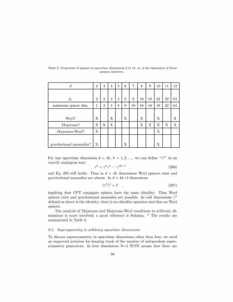
Table 2: Properties of spinors in spacetime dimensions 2 to 12. dγ is the dimension of Diracgamma matrices.
d 2 3 4 5 6 7 8 9 10 11 12
dγ 2 2 4 4 8 8 16 16 32 32 64
minimum spinor dim. 1 2 4 8 8 16 16 16 16 32 64
Weyl? X X X X X X
Majorana? X X X X X X X X
Majorana-Weyl? X X
gravitational anomalies? X X X
For any spacetime dimension d = 4k, k = 1, 2, . . ., we can define “γ5” in anexactly analogous way:
γ5 = γ0γ1 · · · γ4k−1 , (206)
and Eq. 205 still holds. Thus in d = 4k dimensions Weyl spinors exist andgravitational anomalies are absent. In d = 4k+2 dimensions
(γ5)2 = I , (207)
implying that CPT conjugate spinors have the same chirality. Thus Weylspinors exist and gravitational anomalies are possible. In odd dimensions γ5
defined as above is the identity; there is no chirality operator and thus no Weylspinors.
The analysis of Majorana and Majorana-Weyl conditions in arbitrary di-mensions is more involved; a good reference is Sohnius. 4 The results aresummarized in Table 2.
9.2 Supersymmetry in arbitrary spacetime dimensions
To discuss supersymmetry in spacetime dimensions other than four, we needan improved notation for keeping track of the number of independent super-symmetry generators. In four dimensions N=1 SUSY means that there are
50

four independent SUSY generators:
Q1, Q2, Q1, Q2 .
This is of course the minimum number of supersymmetries in four dimensionssince the minimum spinor dimension is four. Let us refer to this as N=(1)4 su-persymmetry. More generally, N=(p)p∗nmin
denotes p ∗ nmin supersymmetries,where nmin is the minimum spinor dimension.
In this new notation the possible global supersymmetries in four dimen-sions are:
N = (1)4
N = (2)8
N = (4)16
N = (8)32
. . .
In 4k+2 dimensions we can have independent chiral and antichiral SUSYgenerators, since CPT conjugates have the same chirality. Thus we need anotation which distinguishes chiral from antichiral SUSY generators:
N = (p, q)(p+q)∗nmin
where p, q are the number of chiral/antichiral SUSY generators, respectively.From Table 2 it is clear that in any spacetime dimension there is a mini-
mum number of supersymmetries (other than zero). Thus:
As few as 4 supersymmetries can only occur for: . . . . . . . . . d ≤ 4
As few as 8 supersymmetries can only occur for: . . . . . . . . . d ≤ 6
As few as 16 supersymmetries can only occur for: . . . . . . . . . d ≤ 10
As few as 32 supersymmetries can only occur for: . . . . . . . . . d ≤ 11
Furthermore, in any spacetime dimension, the maximum number of su-persymmetries of physical interest is always 32 or less. This is because for morethan 32 supersymmetries all massless multiplets contain unphysical higher spinparticles, i.e. particles with spin greater than that of the d-dimensional gravi-ton.
51

Clearly we expect that many SUSY theories in different spacetime dimen-sions but with the same number of supersymmetries can be related, presumablythrough some form of dimensional reduction or truncation. Indeed this is trueas we will see in several examples. Of particular interest is the possibility ofrelating models with extended supersymmetry in four dimensions to simplermodels in the “mother” dimensions 6, 10, and 11.
9.3 Supersymmetry in 2 dimensions
In two dimensions we have (p, q) type superalgebras. I will briefly describesome examples.
• (1, 0)1 supersymmetry: here we have a single left-handed Majorana-Weylspinor:
Q+ = Q†+ ,
Q+, Q+ = 2iPz , (208)
[Q+, Pz ] = [Q+, Pz ] = 0 , (209)
where the antihermitian generators Pz , Pz generate left and right-movingtranslations in the two-dimensional spacetime parameterized by coor-dinates z, z = x0 ± x1. The minimal SUSY multiplet has just twostates: one left-moving real scalar (a “chiral boson”), and one left-movingMajorana-Weyl fermion.
• (1, 1)2 supersymmetry: here we can construct a (1, 1) supersymmetricnonlinear sigma model by supersymmetrizing
∫
dzdz gij(A)∂zAi∂zA
j . (210)
The target spaces of such models are general Riemannian manifolds.
• (2, 2)4 supersymmetry: here again we can construct a supersymmetricnonlinear sigma model. The target spaces are Kahler manifolds. Notethat this agrees with the four-dimensional N=(1)4 case, which has thesame number of supersymmetries.
• (4, 4)8 supersymmetry: here we have supersymmetric nonlinear sigmamodels whose target spaces are hyperKahler manifolds. Again this agreeswith the four-dimensional N=(2)8 case, which has the same number ofsupersymmetries.
52

Two-dimensional supersymmetry has important applications to superstringtheory, where it is interpreted as worldsheet supersymmetry rather thanspacetime SUSY. For more details see Hirosi Ooguri’s lectures in this volume.
9.4 Supersymmetry in 6 dimensions
In six dimensions the minimal case is N=(1,0)8 or (0,1)8. The SUSY generatorscan be expressed as a single complex Weyl spinor:
Qa , a = 1, . . . 8;
Qa, Qb =
1
2(1 + γ7)c
a(γM )bcPM , (211)
where we use capital Roman letters to denote 6-dimensional spacetime indices,and γ7 is the chirality operator, i.e. the 6-dimensional version of “γ5”.
In six dimensions massless particles are labelled by irreps of the little groupSpin(4) ∼ SU(2)×SU(2). Let us describe the possible massless irreps of (0,1)8supersymmetry in terms of their SU(2)×SU(2) “helicity” states:
• hypermultiplet: 2(12 , 0) + 4(0, 0), i.e. one complex Weyl fermion and
two complex scalars, for a total of 4+4 = 8 real components.
• vector multiplet: (12 ,
12 ) + 2(0, 1
2 ), i.e. a massless vector and one com-plex anti-Weyl fermion, for a total of 4+4 = 8 real components.
• gravity multiplet: (1, 1)+2(12 , 1)+(0, 1), i.e. a graviton, two gravitini,
and one self-dual 2nd rank antisymmetric tensor, for a total of 9+12+3 =24 real components.
• tensor multiplet: (1, 0)+2(12 , 0)+(0, 0), i.e. one anti-self-dual 2nd rank
antisymmetric tensor, one complex Weyl fermion, and one real scalar“dilaton”, for a total of 3+4+1 = 8 real components.
Dimensional reduction 6 → 4
Consider six-dimensional N=(0,1)8 supersymmetric Yang-Mills theory. Wewrite the action in terms of fields describing the on-shell massless vector mul-tiplet described above. The action is:
∫
d6x[
− 1
4FMNF
MN +1
2iλγM ∇M λ
]
, (212)
where ∇M is a gauge covariant derivative.
53

Now we imagine compactifying this theory on a torus. Let x4, x5 bethe compactified coordinates. Then the 6-dimensional gauge field AM breaksup into a 4-dimensional gauge field Am and two real scalars A4, A5. Thecomplex anti-Weyl fermion λ breaks up into two 4-dimensional complex Weylfermions. In addition we will have an infinite tower of massive Kaluza-Kleinstates, corresponding to the Fourier decomposition
φ(xm, x4, x5) =∑
n4,n5
e[−in4m4x4−in5m5x5]φn4n5(xm) , (213)
where φ(xm, x4, x5) denotes any 6-dimensional field component, and m4, m5
are inversely related to the compactification radii.The SUSY generator Qa splits up into two Qα’s, implying that the 4-
dimensional theory has N=2 supersymmetry. The 6-dimensional translationgenerator PM splits into Pm, P4, P5. From the 6-dimensional SUSY algebrawe see that P4 and P5 commute with the Qα’s and with Pm. They also appearon the right-hand side of Q,Q. Clearly what we have here are two real =one complex central charge:
Xab ∼ (P4 + iP5)ǫab .
Multiplying the two Qαs by a phase to convert to Zumino’s basis (see Eq. 35),this corresponds to a single real central charge
Z =√
P 24 + P 2
5 . (214)
Thus the dimensionally reduced theory consists of 4-dimensional N=2 super-symmetric Yang-Mills with central charges and an infinite number of massivemultiplets.
Now suppose we repeat the above excercise, but first adding some masslessd = 6 hypermultiplets (A,B, ψ) to our N=(0,1)8 supersymmetric Yang-Millstheory. Each d = 6 hypermultiplet will give one d = 4 multiplet of fieldswith the counting of the d = 4 N=2 massless hypermultiplet, plus a towerof additional massive multiplets. The 6-dimensional on-shell condition for thecomplex scalars A and B
∂M∂MA = ∂M∂MB = 0 (215)
fixes the masses of the 4-dimensional hypermultiplet scalars:
4m2 = Z2 . (216)
Thus the dimensionally reduced theory contains massive BPS-saturated N=2short multiplets, which as already noted do indeed have the same counting asthe d = 4 N=2 massless hypermultiplet.
54

Anomaly cancellation
A striking feature of the 6-dimensional gravity multiplet is that it contains theself-dual part of a 2nd rank antisymmetric tensor, without the anti-self-dualpart. As is also the case in four dimensions, it is impossible to write a Lorentzcovariant Lagrangian formulation of just the self-dual antisymmetric tensorfield. However one can write Lorentz covariant equations of motion, and itappears that the corresponding field theory exists and is Lorentz invariant,despite the lack of a manifestly Lorentz invariant action principle. If
ng = nt = 1 , (217)
where ng, nt are the number of gravity and tensor multiplets, then of coursewe can write a Lorentz covariant Lagrangian. Thus we have the interestingresult that every 6-dimensional supergravity theory either contains a dilatonfield or has no manifestly Lorentz invariant action principle.
In six dimensions we have both gravitational anomalies and mixed gauge-gravitational anomalies. Anomaly cancellation is a severe constraint on theparticle content, and in particular on which combinations of SUSY multipletsyield anomaly-free theories.
For example, when ng=nt=1, the necessary and sufficient condition foranomaly cancellation is:
nh = nv + 244 , (218)
where nh, nv are the number of hypermultiplets and vector multiplets. Thus wealways need a remarkably large number of hypermultiplets to cancel anomalies.
Let’s look at two examples of anomaly-free 6-dimensional N=(0,1)8 super-symmetric supergravity-Yang-Mills-matter theories.
• Gauge group E8 ×E7, with 10 massless hypermultiplets in the (1, 56) ofE8 × E7, and 65 singlet hypermultiplets. Thus:
nv = 248 + 133 = 381 ;
nh = 560 + 65 = 625 ; (219)
which satisfies Eq. 218.
• Gauge group SO(28) × SU(2), with 10 massless hypermultiplets in the(28, 2) of SO(28) × SU(2), and 65 singlet hypermultiplets. Thus:
nv = 378 + 3 = 381 ;
nh = 560 + 65 = 625 ; (220)
which satisfies Eq. 218.
55
These examples arise as compactifications of the ten-dimensional E8 ×E8 and SO(32) heterotic strings, respectively, onto the complex dimension 2Kahler manifold K3.
9.5 Supersymmetry in 11 dimensions
Eleven is the maximum dimension in which we can have as few as 32 super-symmetries. Thus d = 11 is the maximum dimension of interest to supersym-metry theorists, unless one is willing to make some drastic assumptions suchas altering the Minkowski signature of spacetime.
Futhermore, there is only one sensible supersymmetric theory in elevendimensions: N=1 supergravity. The N=(1)32 SUSY algebra is generated by asingle Majorana spinor Qa, a = 1, . . . 32.
Here is the field content of the on-shell massless d = 11 N=1 gravitymultiplet, characterized by irreps of the little group SO(9):
• eAM , the 11-dimensional vielbein. On-shell this constitutes a 44 of SO(9).
• ψaM , a = 1, . . . 32, an 11-dimensional massless vector-spinor, i.e. the
gravitino field. On-shell this is a 128 of SO(9).
• AMNP , a 3rd rank antisymmetric tensor. On-shell this is an 84 of SO(9).
The Lagrangian of 11-dimensional supergravity, in terms of these compo-nent fields of the on-shell multiplet, is rather simple. 24 The first three termsare:
− 1
2κ2eR− 1
2eψMΓMNPDNψP − 1
48eFMNPQF
MNPQ , (221)
where:
κ = 11-dimensional gravitational coupling ,
e ≡ det eAM ,
R = Ricci scalar ,
ΓMNP = eMA eN
B ePC γ
[AγBγC] ,
DN = Lorentz covariant derivative for 11-dim. vector-spinors ,
FMNPQ = ∂[MANPQ], i.e. a field strength ,
and the square brackets denote antisymmetrization.Eleven-dimensional supergravity is the field theory limit of M-theory,
which is in turn a strong coupling limit of superstring theory.
56

Dimensional reductions of d = 11 supergravity
We can truncate d = 1 supergravity down to a 4-dimensional theory by sim-ply suppressing the dependence on x4-x10. Since the resulting 4-dimensionaltheory still has 32 supersymmetries, we obviously must get N=(8)32 extendedsupergravity. Provided one is satisfied with on-shell formulations, this is asimpler way of deriving the rather complicated 4-dimensional theory.
Another useful example is to truncate d = 11 to d = 10. The Majo-rana spinor Qa (32 components) splits into two 10-dimensional Majorana-Weylspinors Qα, Qα (16 components each) with opposite chirality. Thus the trun-cated theory is a nonchiral d = 10 N=(1,1)32 supergravity, commonly knownas Type IIA supergravity. 25
The components of the 11-dimensional vielbein break up as follows:
eAM →
(
eAM AM
0 φ
)
, (222)
where we have set the 1×10 block on the lower left to zero using the freedom ofthose local Lorentz transformations which mix the x11 direction with the otherten. The 10-dimensional massless vector AM arises from the e11M componentsof the vielbein, while the real scalar φ (the 10-dimensional dilaton) arises fromthe e1111 component.
The 11-dimensional antisymmetric tensor field AMNP splits into a 10-dimensional 3rd rank antisymmetric tensor AMNP and a 2nd rank antisym-metric tensor BMN (from AMN11). The 11-dimensional gravitino field ψa
M
becomes:ψa
M → ψαM , ψα
M , λα, λα ; (223)
giving two 10-dimensional Majorana-Weyl vector-spinors of opposite chirality,and two 10-dimensional Majorana-Weyl spinors of opposite chirality.
Since Type IIA supergravity is vectorlike it is trivially free of gravitationalanomalies. It is the field theory limit of the Type IIA superstring.
9.6 More on supersymmetry in 10 dimensions
Type IIA supergravity has N=(1,1)32 supersymmetry. Since 16 is the minimumspinor dimension in ten dimensions, we can in principle construct a chiralN=(1,0)16 supergravity theory as well; however such a theory has gravitationalanomalies. The only other possibility in ten dimensions is a chiral N=(2,0)32supergravity. This theory, known as Type IIB supergravity, turns out tobe anomaly-free, due to highly nontrivial cancellations. Type IIB cannot beobtained by dimensional reduction of 11-dimensional supergravity.
57

Table 3: Comparison of Type II supergravities.
Type IIA: 1 28 35v 8v 56v
φ BMN eAM AM AMNP
8c 8s 56s 56c
λ λ ψ ψ
Type IIB: 1 28 35v 1 28 35c
A AMN eAM A AMN AMNPQ
8s 8s 56s 56s
λ λ ψ ψ
N=(2,0)32 supersymmetry is generated by two Majorana-Weyl spinors Qα,Qα of the same chirality. The on-shell Type IIB supergravity multiplet hasthe following field content:
• eAM , the 10-dimensional vielbein.
• AMNPQ, a self-dual 4th rank antisymmetric tensor.
• AMN , AMN , 2nd rank antisymmetric tensors.
• A, A, real scalars.
• ψαM , ψα
M , Majorana-Weyl vector-spinors of the same chirality.
• λα, λα, Majorana-Weyl spinors of the same chirality.
Because the field content includes the self-dual part of a 4th rank antisymmetrictensor, Type IIB supergravity does not have a Lorentz covariant Lagrangianformulation.
The little group in 10-dimensions is SO(8). Because of the special auto-morphism symmetry of the Lie algebra D4, all of the dimension< 224 irrepsexcept the adjoint occur as triplets of irreps with the same dimension and in-dex. These irreps are distinguished by subscripts v, s, and c. Thus we can gainmore information about the differences between Type IIA and Type IIB su-pergravity by listing the SO(8) irreps corresponding to each component field.Note that both theories have 128+128 = 256 real field components.
58
Let us consider again 10-dimensional N=(1,0)16 supergravity, also knownas Type I supergravity. As we have noted, this theory is anomalous. Re-markably though, by coupling this theory to the 10-dimensional supersymmet-ric Yang-Mills multiplet, we can in certain cases obtain theories free of bothgravitational and mixed gauge-gravitational anomalies. The field content ofthe chiral supergravity is just a truncation of the Type IIA fields:
eAM , BMN , φ ;
ψαM , λα ;
for a total of 64+64 = 128 real field components. The 10-dimensional on-shellN=(1,0)16 supersymmetric Yang-Mills multiplet consists of a massless vectorand a massless Majorana-Weyl spinor
AM , χα ,
in the 8v and 8c irreps of the little group, and the adjoint representation ofsome gauge group.
The details 26 of how to couple N=(1,0) supergravity to N=(1,0) Yang-Mills, consistent with both local supersymmetry and gauge invariance, is be-yond the scope of these lectures. We merely note that one surprising resultis that the gauge invariant field strength of the massless antisymmetric tensorfield BMN has an extra contribution which is a functional of the Yang-Millsgauge field AM . Then, even though BMN is a gauge singlet, gauge invariancerequires that BMN transforms nontrivially under Yang-Mills gauge transfor-mations. This strange fact makes possible the Green-Schwarz anomaly cancel-lation mechanism.
The coupled d = 10 supergravity-Yang-Mills theory is anomaly-free onlyfor the following choices of gauge group:
SO(32), E8 × E8, E8 × [U(1)]248, [U(1)]496 .
The first two choices correspond to the field theory limits of the SO(32) andE8×E8 heterotic strings; the other two choices can probably also be connectedto superstring theory using D-brane arguments.
10 Conclusion
It is a remarkable fact that many technical SUSY topics, thought until recentlyto be of purely academic interest, have turned out to be crucial to obtainingdeep insights about the physics of strongly-coupled nonabelian gauge theories
59

and strongly-coupled string theory. Even if there is no weak scale SUSY in thereal world – even if there is no SUSY at all – supersymmetry has earned itsplace in the pantheon of Really Good Ideas. Furthermore, we are encouragedto continue to develop and expand the technical frontiers of supersymmetry,confident both that there is still much to learn, and that this new knowledgewill find application to important physical problems.
Acknowledgments
The author is grateful to the TASI organizers for scheduling his lectures at 9a.m, to Jeff Harvey for keeping me apprised of the Bull’s playoff schedule, andto Persis Drell for explaining to me what a minimum bias event is. Fermilabis operated by the Universities Research Association, Inc., under contract DE-AC02-76CH03000 with the U.S. Department of Energy.
Appendix
Notation and conventions
My notation and conventions in these lectures conforms with Wess and Bagger2
with the following exceptions:
• I use the standard “West Coast” metric:
ηmn =
1−1
−1−1
(224)
This is the standard metric convention of particle physics. Wess andBagger use the East Coast metric still popular with relativists and otherbenighted souls.
Changes which follow from my different choice of metric:
1. My σ0 and σ0 are the 2x2 identity matrix instead of minus it.
2. I define the SL(2,C) generators with an extra factor of i:
σmnα
β =i
4
[
σmαγ σ
nγβ − σnαγ σ
mγβ]
. (225)
3. I define the Levi-Civita tensor density ǫ0123 = +1 instead of minusone.
60

4. As a result of this, σmn is self-dual and σmn is anti-self-dual, insteadof vice-versa.
5. In the full component expansion of the chiral superfield Φ(x, θ, θ),the (θθ)(θθ) term comes in with the opposite sign.
Spinor definitions and identities
Irreps of SL(2,C) ≈ SO(1,3):
(1
2, 0) = left−handed 2 component Weyl spinor
(0,1
2) = right−handed 2 component Weyl spinor
In Van der Waerden notation, undotted = (12 , 0), dotted = (0, 1
2 ):
(1
2, 0) : ψα ,
(0,1
2) : ψα ≡ (ψα)∗ .
Also:
ψα ≡ (ψα)† ; ψα ≡ (ψα)∗ . (226)
We raise and lower spinor indices with the 2-dimensional Levi-Civita symbols:
ǫαβ = ǫαβ =
(
0 −11 0
)
;
ǫαβ = ǫαβ =
(
0 1−1 0
)
= iσ2 . (227)
Thus:
ψα = ǫαβψβ ; ψα = ǫαβψβ ;
ψα = ǫαβψβ ; ψα = ǫαβψβ . (228)
Note also:
61

ǫαβǫβγ = δγ
α ,
ǫαβǫβγ = δγ
α , (229)
ǫαβǫδγ = δγ
αδδβ − δδ
αδγβ ,
ǫαβǫδγ = δγ
αδδβ− δδ
αδγ
β.
Pauli Matrices:
σ1 =
(
0 11 0
)
σ2 =
(
0 −ii 0
)
σ3 =
(
1 00 −1
)
(230)
From which we define:
σm = (I, ~σ) = σm ,
σm = (I,−~σ) = σm , (231)
where I denotes the 2x2 identity matrix. Note that in these definitions “bar”does not indicate complex conjugation.
σm has undotted-dotted indices: σmαβ
σm has dotted-undotted indices: σmαβ
We also have the completeness relations:
trσmσn = 2ηmn ,
σmαβσγδ
m = 2δδαδ
γ
β. (232)
σm and σm are related by the Levi-Civita symbols:
σmαβ = ǫαγǫβδσmδγ ; σm
αβ= ǫδβǫγασ
mδγ . (233)
It is occasionally convenient to do a “fake” conversion of an undotted to adotted index or vice versa using the fact that σ0 and σ0 are just the identitymatrix:
ψα = (ψβ)∗σ0βα ; ψα = (ψβ)∗σ0βα . (234)
62

Because the Pauli matrices anticommute, i.e.
σi, σj = δijI i, j = 1, 2, 3 (235)
we have the relations:
(σmσn + σnσm)βα = 2ηmnδβ
α ,
(σmσn + σnσm)βα = 2ηmnδβ
α . (236)
Spinor Summation Convention:
ψχ = ψαχα = −ψαχα = χαψα = χψ
ψχ = ψαχα = −ψαχα = χαψ
α = χψ (237)
Note that these quantities are Lorentz scalars.We also have:
(χψ)† = (χαψα)† = ψαχα = χψ
(χσmψ)† = ψσmχ = Lorentz vector (238)
Other useful relations are:
ψαψβ = − 1
2ǫαβψψ ,
ψαψβ =1
2ǫαβψψ , (239)
ψαψβ =1
2ǫαβψψ ,
ψαψβ = − 1
2ǫαβψψ .
The SL(2,C) generators are defined as
σmnα
β =i
4
[
σmαγ σ
nγβ − σnαγ σ
mγβ]
σmnαβ =
i
4
[
σmαγσnγβ
− σnαγσmγβ
]
(240)
63
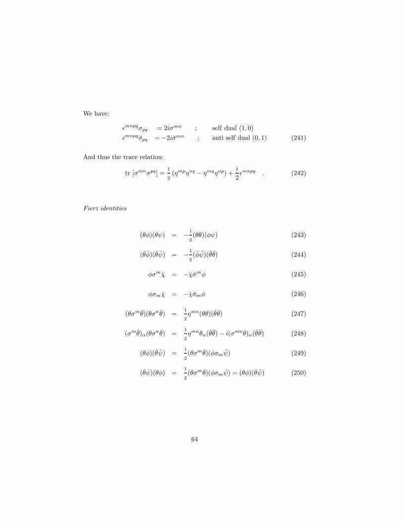
We have:
ǫmnpqσpq = 2iσmn ; self dual (1, 0)
ǫmnpqσpq = −2iσmn ; anti self dual (0, 1) (241)
And thus the trace relation:
tr [σmnσpq] =1
2(ηmpηnq − ηmqηnp) +
i
2ǫmnpq . (242)
Fierz identities
(θφ)(θψ) = − 1
2(θθ)(φψ) (243)
(θφ)(θψ) = − 1
2(φψ)(θθ) (244)
φσmχ = −χσmφ (245)
φσmχ = −χσmφ (246)
(θσmθ)(θσn θ) =1
2ηmn(θθ)(θθ) (247)
(σmθ)α(θσnθ) =1
2ηmnθα(θθ) − i(σmnθ)α(θθ) (248)
(θφ)(θψ) =1
2(θσmθ)(φσmψ) (249)
(θψ)(θφ) =1
2(θσmθ)(φσmψ) = (θφ)(θψ) (250)
64

General 4-dimensional SUSY algebra
QAα , QβB = 2σm
αβPmδ
AB (251)
QAα , Q
Bβ = ǫαβa
ℓABBℓ (252)
QαA, QβB = −ǫαβa∗ℓABB
ℓ (253)
[QAα , Pm] = [Q
A
α , Pm] = 0 (254)
[QAα ,Mmn] = σmnα
βQAβ (255)
[Qα
A,Mmn] = σαmnβQ
β
A (256)
[Pm, Pn] = 0 (257)
[Mmn, Pp] = i(ηnpPm − ηmpPn) (258)
[Mmn,Mpq] = −i(
ηmpMnq − ηmqMnp
−ηnpMmq + ηnqMmp
)
(259)
[QAα , Bℓ] = SA
ℓ BQBα (260)
[QαA, Bℓ] = −S∗ℓA
BQαB (261)
[Bℓ, Bk] = iCℓkjBj (262)
[Pm, Bℓ] = [Mmn, Bℓ] = 0 (263)
Where the aℓ are antisymmetric matrices, and Sℓ, aℓ must satisfy the inter-twining relation:
SAℓ C aCBk = −aACk S∗ℓ
C
B(264)
65

Note also the perverse but essential convention implicit in Wess and Bagger:
aℓAB = −aℓAB (265)
N=1 SUSY algebra in 4 dimensions
Qα, Qβ = 2σmαβPm (266)
Qα, Qβ = Qα, Qβ = 0 (267)
[Qα, Pm] = [Qα, Pm] = 0 (268)
[Qα,Mmn] = σmnαβQβ (269)
[Qα,Mmn] = σα
mnβQβ
(270)
[Pm, Pn] = 0 (271)
[Mmn, Pp] = i(ηnpPm − ηmpPn) (272)
[Mmn,Mpq] = −i (ηmpMnq − ηmqMnp − ηnpMmq + ηnqMmp)(273)
[Qα, R] = RQα (274)
[Qα, R] = −RQα (275)
[Pm, R] = [Mmn, R] = 0 (276)
References
1. J. Amundson et al, “Report of the Supersymmetry Theory Subgroup”,hep-ph/9609374; S. Dawson, “SUSY and Such”, hep-ph/9612229; M.Drees, “An Introduction to Supersymmetry”, hep-ph/9611409; J. Bag-ger, “Weak Scale Supersymmetry: Theory and Practice”, Lectures atTASI 95, hep-ph/9604232; X. Tata, “Supersymmetry: Where it is andHow to Find it”, Talk at TASI 95, hep-ph/9510287; H. Baer et al, “Low-energy Supersymmetry Phenomenology”, hep-ph/9503479.
2. Supersymmetry and Supergravity, J. Wess and J. Bagger (2nd edi-tion, Princeton University Press, Princeton NJ, 1992.)
3. Introduction to Supersymmetry and Supergravity, Peter West(2nd edition, World Scientific, Singapore, 1990.)
4. M. Sohnius, Introducing Supersymmetry, Phys. Rep. 128, 39(1985).
5. N. Seiberg and E. Witten, Nucl. Phys. B 426, 19 (1994).6. S. Coleman and J. Mandula, Phys. Rev. 159, 1251 (1967).7. R. Haag, J. Lopuszanski, and M. Sohnius, Nucl. Phys. B 88, 257 (1975).
66

8. For an interesting attempt, see H. van Dam and L. Biedenharn, Phys.
Lett. B 81, 313 (1979).9. B. Zumino, J. Math. Phys. 3, 1055 (1962).
10. See Jeff Harvey’s lectures in this volume.11. S. Ferrara, C. Savoy, and B. Zumino, Phys. Lett. B 100, 393 (1981).12. S. Ferrara and B. Zumino, Nucl. Phys. B 79, 413 (1974).13. M. Grisaru, M. Rocek, and W. Siegel, Nucl. Phys. B 159, 429 (1979).14. J. Wess and B. Zumino, Nucl. Phys. B 70, 39 (1974).15. D. Friedan, Phys. Rev. Lett. 45, 1057 (1980); M. Rocek, Physica D 15,
75 (1985).16. B. Zumino, Phys. Lett. B 87, 203 (1979).17. R. Grimm, M. Sohnius, and J. Wess, Nucl. Phys. B 133, 275 (1978); A.
Galperin, E. Ivanov, S Kalitzin, V. Ogievetsky, and E. Sokatchev, Class.
Quant. Grav. 1, 469 (1984); N. Ohta, H. Sugata, and H. Yamaguchi,Annals of Physics 172, 26 (1986); P. Howe, “Twistors and Supersymme-try”, hep-th/9512066.
18. A. Strominger, Commun. Math. Phys. 133, 163 (1990).19. L. Alvarez-Gaume and D. Freedman, Commun. Math. Phys. 80, 443
(1981).20. P. van Nieuwenhuizen, Supergravity, Phys. Rep. 68, 189 (1981).21. N. Seiberg, Phys. Lett. B 206, 75 (1988).22. M. Shifman and A. Vainshtein, Nucl. Phys. B 277, 456 (1986).23. L. Alvarez-Gaume and E. Witten, Nucl. Phys. B 234, 269 (1983).24. E. Cremmer, B. Julia, and J. Scherk, Phys. Lett. B 76, 409 (1978).25. Superstring Theory, M. Green, J. Schwarz, and E. Witten (Cambridge
University Press, Cambridge, 1987.)26. G. Chapline and N. Manton, Phys. Lett. B 120, 105 (1983).
67


![APlanck-scaleaxionandSU(2)Yang-Millsdynamics ... · 2 SU(2) Yang-Mills thermodynamics In [12] a nonperturbative approach for SU(2)/SU(3) Yang-Mills thermodynamics is developed. For](https://img.pdfslide.us/doc/110x75/5e177a861854e443044d43a2/aplanck-scaleaxionandsu2yang-millsdynamics-2-su2-yang-mills-thermodynamics.jpg)