Embed Size (px)
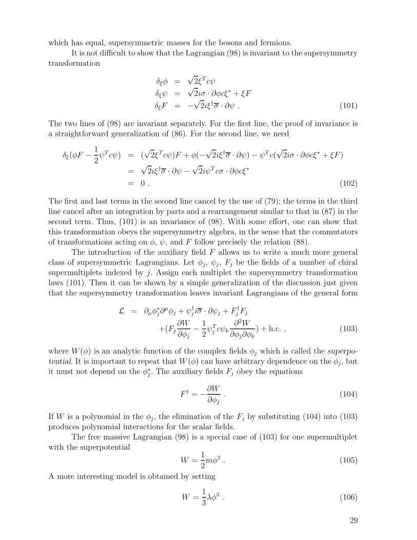
Citation preview
arX
iv:h
ep-p
h/97
0547
9v1
30
May
199
7
SLAC-PUB-7479May, 1997
Beyond the Standard Model
Michael E. Peskin1)
Stanford Linear Accelerator Center
Stanford University, Stanford, California 94309 USA
ABSTRACT
These lectures constitute a short course in ‘Beyond the Standard Model’ for
students of experimental particle physics. I discuss the general ideas which guidethe construction of models of physics beyond the Standard Model. The central
principle, the one which most directly motivates the search for new physics, is thesearch for the mechanism of the spontaneous symmetry breaking observed in the
theory of weak interactions. To illustrate models of weak-interaction symmetrybreaking, I give a detailed discussion of the idea of supersymmetry and that of
new strong interactions at the TeV energy scale. I discuss experiments that willprobe the details of these models at future pp and e+e− colliders.
to appear in the proceedings of the1996 European School of High-Energy Physics
Carry-le-Rouet, France, September 1–14, 1996
1) Work supported by the Department of Energy, contract DE–AC03–76SF00515.

1

BEYOND THE STANDARD MODEL
Michael E. Peskin
SLAC, Stanford University, Stanford, California USA
Abstract
These lectures constitute a short course in ‘Beyond the Standard
Model’ for students of experimental particle physics. I discuss thegeneral ideas which guide the construction of models of physics
beyond the Standard Model. The central principle, the one whichmost directly motivates the search for new physics, is the search for
the mechanism of the spontaneous symmetry breaking observedin the theory of weak interactions. To illustrate models of weak-
interaction symmetry breaking, I give a detailed discussion of theidea of supersymmetry and that of new strong interactions at the
TeV energy scale. I discuss experiments that will probe the detailsof these models at future pp and e+e− colliders.
1. Introduction
Every year, the wise people who organize the European School of Particle Physics
feel it necessary to subject young experimentalists to a course of lectures on ‘Beyond theStandard Model’. They treat this subject as if it were a discipline of science that one
could study and master. Of course, it is no such thing. If we knew what lies beyond theStandard Model, we could teach it with some confidence. But the interest in this subject
is precisely that we do not know what is waiting for us there.The confusion about ‘Beyond the Standard Model’ goes beyond students and sum-
mer school organizers to the senior scientists in our field. A theorist such as myself whoclaims to be able to explain things about physics beyond the Standard Model is very of-
ten met with skepticism that such explanations are even possible. ‘Do we really have any
idea’, one is told, ‘what we will find a higher energies?’ ‘Don’t we just want the highestpossible energy and luminosity?’ ‘The Standard Model works very well, so why must there
be any new physics at all?’And yet there are specific things that one can teach that should be relevant to
physics beyond the Standard Model. Though we do not know what physics to expect athigher energies, the principles of physics that we have learned in the explication of the
Standard Model should still apply there. In addition, we hope that some of the questions
1
not answered by the Standard Model should be answered there. This course will concen-
trate its attention on these two issues: What questions are likely to be addressed by new
physics beyond the Standard Model, and what general methods of analysis can we use tocreate and analyze proposed answers to these questions?
A set of lectures on ‘Beyond the Standard Model’ should have one further goalas well. It is possible that the first sign of physics beyond the Standard Model could be
discovered next year at LEP, or perhaps it is already waiting in the unanalyzed data fromthe Fermilab collider. On the other hand, it is possible that this discovery will have to wait
for the great machines of the next generation. Many people feel dismay at the fact that thepace of discovery in high-energy physics is very slow, with experiments operating on the
time scale of a decade familiar in planetary science rather than on the time scale of daysor weeks. Because of the cost and complexity of modern elementary particle experiments,
these long time scales are inevitable, and we have to adjust our expectations to them. Butthe long time scales also require that we set for ourselves very clear goals that we can try
to realize a decade in the future. To do this, it is useful to have a concrete understandingof what experiments will look like at the next generation of colliders and what physics
issues they address. Even if we cannot correctly predict what Nature will provide for us
at higher energy, it is essential to take some models as illustrative examples and work outin complete detail how to analyze them experimentally. With luck, we can choose models
will have features relevant to the ultimate correct theory of the next scale in physics. Buteven if we are not sufficiently lucky or insightful to predict what will appear, such a study
will leave us prepared to solve whatever puzzles Nature has set.This, then, is what I would like to accomplish in these lectures. I will set out
some questions which I feel are the most important ones at the present stage of ourunderstanding, and the ones which I feel are most likely to be addressed by the new
phenomena of the next energy scale. I will explain some theoretical ideas that have comefrom our understanding of the Standard Model that I feel will play an important role at
the next level. Building on these ideas, I will describe illustrative models of physics beyondthe Standard Model. And, for each case, I will describe the program of experiments that
will clarify the nature of the new physics that the model implies.When we design a program of future high-energy experiments, we are also calling
for the construction of new high-energy accelerators that would be needed to carry out this
program. I hope that students of high-energy physics will take an interest in this practicalor political aspect of our field of science. Those who think about this seriously know that
we cannot ask society to support such expensive machines unless we can promise that thesefacilities will give back fundamental knowledge that is of the utmost importance and that
cannot be obtained in any other way. I hope that they will be interested to see how centrala role the CERN Large Hadron Collider (LHC) plays in each of the experimental programs
that I will describe. Another proposed facility will also play a major role in my discussion,a high-energy e+e− linear collider with center-of-mass energy about 1 TeV. I will argue in
these lectures that, with these facilities, the scientific justification changes qualitativelyfrom that of the present colliders at CERN and Fermilab. Whereas at current energies,
we search for new physics and try to place limits, at next step in energy we must find newphysics that addresses one of the major gaps in the Standard Model.
This last issue leads to us to ask another, and perhaps unfamiliar, question about
2
the colliders of the next generation. Much ink has been wasted in comparing hadron and
lepton colliders on the basis of energy reach and asking which is preferable. The real issue
for these machines is a different one. We will see that illustrative models of new physicsbased on simple ideas will out to have rich and complex phenomenological consequences.
Thus, it is a serious question whether we will be able to understand the model that Naturehas put forward for us from experimental observations. I will argue through my examples
that these two types of colliders, which focus on different and complementary aspects ofthe high-energy phenomena, can bring back a complete picture of the new phenomena of
a clarity that neither, working alone, could achieve.The outline of these lectures is as follows. In Section 2, I will introduce the question
of the mechanism of electroweak symmetric breaking and also two related questions thatinfluence the construction and analysis of models of new physics. In Sections 3 and 4, I
will give one illustrative set of answers to these questions through a detailed discussionof models with supersymmetry at the weak-interaction scale. Section 3 will develop the
formalism of supersymmetry and derive its connection to the questions I have set out.Section 4 will discuss more detailed properties of supersymmetric models which provide
interesting experimental probes. In Section 5, I will discuss models with new strong in-
teractions at the TeV mass scale, models which give very different answers to our broadquestions about physics beyond the Standard Model. In Section 6, I will summarize the
lessons of our study of these two very different types of models and draw some generalconclusions.
2. Three Basic Questions
To begin our study of physics beyond the Standard Model, I will review some
properties of the Standard Model and some insights that it provides. I will also discusssome questions that the Standard Model does not answer, but which might reasonably
be answered at the next scale in fundamental physics.
2.1 Why not just the Standard Model?
To introduce the study of physics beyond the Standard Model, I must first explainwhat is wrong with the Standard Model. To see this, we only have to compare the publicity
for the Standard Model, what we say about it to beginning students and to our colleaguesin other fields, with the explicit expression for the Standard Model Lagrangian.
When we want to advertise the virtues of the Standard Model, we say that itis a model whose foundation is symmetry. We start from the principle of local gauge
invariance, which tells us that the interactions of vector bosons are associated with aglobal symmetry group. The form of these interactions is uniquely specified by the group
structure. Thus, from the knowledge of the basic symmetry group, we can write down
the Lagrangian or the equations of motion. Specifying the group to be U(1), we deriveelectromagnetism. To create a complete theory of Nature, we choose the group, in accord
with observation, to be SU(3) × SU(2) × U(1). This group is a product, and we are freeto include a different coupling constant for each factor. But in the ideal theory, these
would be the only parameters. Specify to which representations of the gauge group thematter particles belong, fix the three coupling constants, and we have a complete theory
of Nature.
3
This set of ideas is tantalizing because it is so close to being true. The couplings
of quarks and leptons to the strong, weak, and electromagnetic interactions are indeed
fixed correctly in terms of three coupling constants. From the LEP and SLC experiments,we have learned that the pattern of weak-interaction couplings of the quarks and leptons
follows the symmetry prediction to the accuracy of a few percent, and also that thestrong-interaction coupling is universal among quark flavors at a similar level of accuracy.
On the other hand, the Lagrangian of the Minimal Standard Model tells a ratherdifferent story. Let me write it here for reference:
L = qi 6Dq + ℓi 6Dℓ− 1
4(F a
µν)2
+ |Dµφ|2 − V (φ)
−(λiju u
iRφ ·Qj
L + λijd di
Rφ∗ ·Qj
L + λijℓ eiRφ
∗ · LjL + h.c.). (1)
The first line of (1) is the pure gauge theory discussed in the previous paragraph.
This line of the Lagrangian contains only three parameters, the three Standard Modelgauge couplings gs, g, g
′, and it does correctly describe the couplings of all species of
quarks and leptons to the strong, weak, and electromagnetic gauge bosons.The second line of (1) is associated with the Higgs boson field φ. The Minimal
Standard Model introduces one scalar field, a doublet of weak interaction SU(2), so thatits vacuum expectation value can give a mass to theW and Z bosons. The potential energy
of this field V (φ) contains at least two new parameters which play a role in determiningthe W boson mass. At this moment, there is no experimental evidence for the existence
of the Higgs field φ and very little evidence that constrains the form of its potential.
The third line of (1) similarly gives an origin for the masses of quarks and lep-tons. In the Standard Model, the left- and right-handed quark fields belong to different
representations of SU(2)×U(1); a similar conclusion holds for the leptons. On the otherhand, a mass term for a fermion couples the left- and right-handed components. This is
impossible as long as the gauge symmetry is exact. In the Standard Model, one can writea trilinear term linking a left- and right-handed pair of species to the Higgs field. When
the Higgs field acquires a vacuum expectation value, this coupling turns into a mass term.Unfortunately, a generic fermion-fermion-boson coupling is restricted only rather weakly
by gauge symmetries. The Standard Model gauge symmetry allows three complex 3 × 3matrices of couplings, the paramaters λij of (1). When φ acquires a vacuum expectation
values, these matrices become the mass matrices of quarks and leptons. Thus, whereasthe gauge couplings of quarks and leptons were strongly restricted by symmetry, the mass
terms for these particles can be of general and, indeed, complex, structure.If we consider (1) to be the fundamental Lagrangian of Nature, the situation is even
worse. The Higgs coupling matrices λij are renormalizable couplings in this Lagrangian.
The property of renormalizability implies that, once these couplings are specified, the the-ory gives definite predictions. However, the specification of the renormalizable couplings is
part of the statement of the problem. Except in very special field theories, these couplingscannot be determined from the internal consistency of the theory itself. The Standard
Model Lagrangian then leaves us with the three matrices λij , and the parameters of theHiggs potential V (φ), as conditions of the problem which cannot in principle be deter-
mined. In order to understand why the masses of the quarks, the leptons, and the W and
4
Z bosons have their observed values, we must find a deeper theory beyond the Standard
Model from which the Lagrangian (1), or some replacement for it, can be derived.
Thus, it is a disappointing feature of the Minimal Standard Model that it has alarge number of parameter which are undetermined, and which cannot be determined.
This disappointment, though, has an interesting converse. Typically in physics, when wemeet a system with a large number of parameters, what stands behind it is a system with a
simple description which is realized with some complexity in its dynamics. The transportcoefficients of fluids or the properties of electrons in a semiconductor are described in
terms of a large number of parameters, but these parameters can be computed froman underlying atomic picture. Through this analogy, we would conclude that the gauge
couplings of quarks and leptons are likely to reflect a fundamental structure, but thatthe Higgs boson is unlikely to be simple, minimal, or elementary. The multiplicity of
undermined couplings of the Minimal Standard Model are precisely those of the Higgsboson. If we could break through and discover the simple underlying picture behind the
Higgs boson, or behind the breaking of SU(2)×U(1) symmetry, we would then have thecorrect deeper viewpoint from which to understand the undetermined parameters of the
Standard Model.
2.2 Three models of electroweak symmetry breaking
The argument given in the previous section leads us to the question: What is
actually the mechanism of electroweak symmetry breaking? In this section, I would liketo present three possible models for this phenomenon and to discuss their strengths and
weaknesses.The first of these is the model of electroweak symmetry breaking contained in the
Minimal Standard Model. We introduce a Higgs field
φ =
(φ+
φ0
)(2)
with SU(2) × U(1) quantum numbers I = 12, Y = 1
2. I will use τa = σa/2 to denote
the generators of SU(2), and I normalize the hypercharge so that the electric charge is
Q = I3 + Y .Take the Lagrangian for the field φ to be the second line of (1), with
V (φ) = −µ2φ†φ+ λ(φ†φ)2 . (3)
This potential is minimized when φ†φ = µ2/2λ. Thus, one particular vacuum state isgiven by
〈φ〉 =
(01√2v
), (4)
where v2 = µ2/λ.
The most general φ field configuration can be written in the same notation as
φ = eiα(x)·τ(
01√2(v + h(x))
). (5)
In this expression, αa(x) parametrizes an SU(2) gauge transformation. The field h(x) is
a gauge-invariant fluctation away from the vacuum state; this is the physical Higgs field.
5
The mass of this field is given by
m2h = 2µ2 = 2λv2 . (6)
Notice that, in this model, h(x) is the only gauge-invariant degree of freedom in φ(x), andso the symmetry-breaking sector gives rise to only one new particle, the Higgs scalar.
If we insert (4) into the kinetic term for φ, we obtain a mass term for W and Z; thisis the usual Higgs mechanism for producing these masses. If g and g′ are the SU(2)×U(1)
coupling constants, one finds the familiar result
mW = gv
2, mZ =
√g2 + g′2
v
2. (7)
The measured values of the masses and couplings then lead to
v = 246 GeV . (8)
This is a very simple model of SU(2) × U(1) symmetry breaking. Perhaps it iseven too simple. If we ask the question, why is SU(2)×U(1) broken, this model gives the
answer ‘because (−µ2) < 0.’ This is a perfectly correct answer, but it teaches us nothing.Normally, the grand qualitative phenomena of physics happen as the result of definite
physical mechanisms. But there is no physically understandable mechanism operatinghere.
One often hears it said that if the minimal Higgs model is too simple, one canmake the model more complex by adding a second Higgs doublet. For our next case, then,
let us consider a model with two Higgs doublets φ1, φ2, both with I = 12, Y = 1
2. The
Lagrangian of the Higgs fields is
L = |Dµφ1|2 + |Dµφ1|2 − V (φ1, φ2) , (9)
with
V = − (φ†1 φ†
2 )M2
(φ1
φ2
)+ · · · , (10)
where M2 is a 2 × 2 matrix. It is not difficult to engineer a form for V such that, at the
minimum, the vacuum expectation values of φ1 and φ2 are aligned:
〈φ1〉 =
(0
1√2v1
), 〈φ2〉 =
(0
1√2v2
). (11)
The ratio of the two vacuum expectation values is conventionally parametrized by an
angle β,
tanβ =v2
v1. (12)
To reproduce the correct values of the W and Z mass,
v21 + v2
2 = v2 = (246 GeV)2 . (13)
The field content of this model is considerably richer than that of the minimalmodel. An infinitesimal gauge transformation of the vacuum configuration (11) leads to
a field configuration
δφ1 =1
2
(v1(α1 + iα2)
v1(iα3)
), δφ2 =
1
2
(v2(α1 + iα2)
v2(iα3)
). (14)
6
The fluctuations of the field configuration which are orthogonal to this lead to new physical
particles. These include the motions
δφ1 =1
2
(sin β · (h1 + ih2)
sin β · (ih3)
), δφ2 =
1
2
(− cos β · (h1 + ih2)
− cos β · (ih3)
), (15)
as well as the fluctuations vi → vi + Hi of the two vacuum expectation values. Thus we
find five new particles. The fields h1 and h2 combine to form charged Higgs bosons H±.The field h3 is a CP-odd neutral boson, usually called A0. The two fields Hi typically mix
to form mass eigenstates called h0 and H0.I have discussed this structure in some detail because we will later see it appear
in specific model contexts. But it does nothing as far as answering the physical questionthat I posed a moment ago. Again, if one asks what is the mechanism of weak interaction
symmetry breaking, the answer this model gives is that the matrix (−M2) has a negativeeigenvalue.
The third model I would like to discuss is a model of a very different kind proposed
in 1979 by Weinberg and Susskind [1, 2]. Imagine that the fundamental interactionsinclude a new gauge interaction which is almost an exact copy of QCD with two quark
flavors. The new interactions differ from QCD in only two respects: First, the quarksare massless; second, the nonperturbative scales Λ and mρ are much larger in the new
subsection. The two flavors of quarks should be coupled to SU(2) × U(1) just as (u, d)are, and I will call them (U,D).
In QCD, the strong interactions between quarks and antiquarks leads to the gen-eration of large effective masses for the u and d. This mass generation is associated with
spontaneous symmetry breaking. The strong interactions between very light quarks andantiquarks make it energetically favorable for the vacuum of space to fill up with quark-
antiquark pairs. This gives vacuum expectation values to operators built from quark andantiquark fields.
The analogue of this phenomenon should occur in our theory of new interactions—for just the same reason—and so we should find
⟨UU
⟩=⟨DD
⟩= −∆ 6= 0 . (16)
In terms of chiral components,
UU = U †LUR + U †
RUL , (17)
and similarly for DD. But, in the weak-interaction theory, the left-handed quark fields
transform under SU(2) while the right-handed fields do not. Thus, the vacuum expectation
value in (16) signals SU(2) symmetry breaking. In fact, under SU(2)×U(1), the operatorQLUR has the same quantum numbers I = 1
2, Y = 1
2as the elementary Higgs boson that
we introduced in our earlier model. The vacuum expectation value of this operator thenhas the same effect: It breaks SU(2) × U(1) to the U(1) symmetry of electromagnetism
and gives mass to the three weak-interaction bosons.I will explain in Section 5.1 that the pion decay constant Fπ of the new strong
interaction theory plays the role of v in (7) in determining the mass scale of mW and mZ .If we were to set Fπ to the value given in (8), we would need to scale up QCD by the
factor246 GeV
93 MeV= 2600. (18)
7
Then the hadrons of these new strong interactions would be at TeV energies.
For me, the Weinberg-Susskind model is much more appealing as a model of elec-
troweak symmetry breaking than the Minimal Standard Model. The reason for this is that,in the Weinberg-Susskind model, electroweak symmetry breaking happens naturally, for
a reason, rather than being included as the result of an arbitrary choice of parameters. Iwould like to emphasize especially that the Weinberg-Susskind model is preferable even
though it is more complex. In fact, this complexity is an essential part of its founda-tion. In this model, something happens, and that physical action gives rise to a set of
consequences, of which electroweak symmetry breaking is one.This notion that the consequences of physical theories flow from their complexity
is familiar from the theories in particle physics that we understand well. In QCD, quarkconfinement, the spectrum of hadrons, and the parton description of high-energy reactions
all flow out of the idea of a strongly-coupled non-Abelian gauge interaction. In the weakinteractions, the V –A structure of weak couplings and all of its consequences for decays
and asymmetries follow from the underlying gauge structure.Now we are faced with a new phenomenon, the symmetry breaking of SU(2)×U(1),
whose explanation lies outside the realm of the known gauge theories. Of course it is
possible that this phenomenon could be explained by the simplest, most minimal additionto the laws of physics. But that is not how we have seen Nature work. In searching for an
explanation of electroweak symmetry breaking, we should not be searching for a simplistictheory but rather for a simple idea from which deep and rich consequences might flow.
2.3 Questions for orientation
The argument of the previous section gives focus to the study of physics beyond the
Standard Model. We have a phenomenon necessary to the working of weak-interaction the-ory, the symmetry-breaking of SU(2)×U(1), which we must understand. This symmetry-
breaking is characterized by a mass scale, v in (8), which is close to the energy scales nowbeing probed at accelerators. At the same time, it is a new qualitative phenomenon which
cannot originate from the known gauge interactions. Therefore, it calls for new physics,and in an energy region where we can hope to discover it. For me, this is the number one
question of particle physics today:* What is the mechanism of electroweak symmetry breaking?
Along with this question come two subsidiary ones. Both of these are connectedto the fact that electroweak symmetry breaking is necessary for the generation of masses
for the weak-interaction bosons, the quarks, and the leptons. Perhaps there are also otherparticles which cannot obtain mass until SU(2) × U(1) is broken. Then these particles
also must have masses at the scale of a few hundred GeV or below. The heaviest of theseparticles must be especially strongly coupled to the fields that are the basic cause of the
symmetry-breaking. At the very least, the top quark belongs to this class of very heavy
particles, and other members of this class might well be found. Thus, we are also led toask,
* What is the spectrum of elementary particles at the 1 TeV energy scale?
* Is the mass of the top quark generated by weak couplings or by new strong
interactions?
In the remainder of this section, I will comment on these three questions. In the
following sections, when we consider explicit models of electroweak symmetry breaking, I
8
will develop the models theoretically to propose answer these questions. At any stage in the
argument, though, you should have firmly in mind that these answers will ultimately come
from experiment, and, in particular, from direct observations of TeV-energy phenomena.The goal of my theoretical arguments, then, will be to suggest particular phenomena
which could be observed experimentally to shed light on these questions. We will see inSections 4 and 5 that models which attempt to explain electroweak symmetry breaking
typically suggest a variety of new experimental probes, which may allow us to uncover awhole new layer of the fundamental interactions.
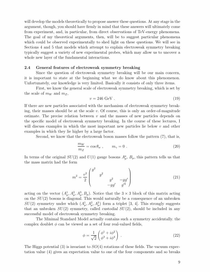
2.4 General features of electroweak symmetry breaking
Since the question of electroweak symmetry breaking will be our main concern,
it is important to state at the beginning what we do know about this phenomenon.Unfortunately, our knowledge is very limited. Basically it consists of only three items.
First, we know the general scale of electroweak symmetry breaking, which is set by
the scale of mW and mZ ,v = 246 GeV . (19)
If there are new particles associated with the mechanism of electroweak symmetry break-
ing, their masses should be at the scale v. Of course, this is only an order-of-magnitudeestimate. The precise relation between v and the masses of new particles depends on
the specific model of electroweak symmetry breaking. In the course of these lectures, Iwill discuss examples in which the most important new particles lie below v and other
examples in which they lie higher by a large factor.Second, we know that the electroweak boson masses follow the pattern (7), that is,
mW
mZ= cos θw , mγ = 0 . (20)
In terms of the original SU(2) and U(1) gauge bosons Aaµ, Bµ, this pattern tells us thatthe mass matrix had the form
m2 =v2
2
g2
g2
g2 −gg′−gg′ g′2
(21)
acting on the vector (A1µ, A
2µ, A
3µ, Bµ). Notice that the 3 × 3 block of this matrix acting
on the SU(2) bosons is diagonal. This would naturally be a consequence of an unbroken
SU(2) symmetry under which (A1µ, A
2µ, A
3µ) form a triplet [3, 4]. This strongly suggests
that an unbroken SU(2) symmetry, called custodial SU(2), should be included in any
successful model of electroweak symmetry breaking.The Minimal Standard Model actually contains such a symmetry accidentally. the
complex doublet φ can be viewed as a set of four real-valued fields,
φ =1√2
(φ1 + iφ2
φ3 + iφ4
). (22)
The Higgs potential (3) is invariant to SO(4) rotations of these fields. The vacuum expec-
tation value (4) gives an expectation value to one of the four components and so breaks
9
SO(4) spontaneously to SO(3) = SU(2). In the Weinberg-Susskind model, there is also a
custodial SU(2) symmetry, the isospin symmetry of the new strong interactions. In this
case, the custodial symmetry is not an accident, but rather a component of the new idea.Third, we know that the new interactions responsible for electroweak symmetry
breaking contribute very little to precision electroweak observables. I will discuss thisconstraint in somewhat more detail in Section 5.2. For the moment, let me point out that,
if we take the value of the electromagnetic coupling α and the weak interaction parametersGF and mZ as input parameters, the value of the weak mixing angle sin2 θw that governs
the forward-backward and polarization asymmetries of the Z0 can be shifted by radiativecorrections involving particles associated with the symmetry breaking. In the Minimal
Standard Model, this shift is rather small,
δ(sin2 θw) =α
cos2 θw − sin2 θw
1 + 9 sin2 θw24π
logmh
mZ
. (23)
The coefficient of the logarithm has the value 6 × 10⁻⁴. The accuracy of the LEP andSLC experiments is such that the size of the logarithm cannot be much larger than 1, and
larger radiative corrections from additional sources are forbidden. In models of electroweaksymmetry breaking based on new strong interactions, this can be an important constraint.
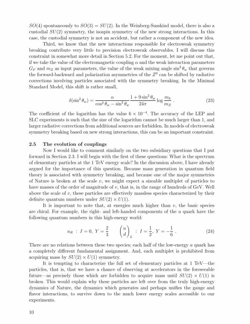
2.5 The evolution of couplings
Now I would like to comment similarly on the two subsidiary questions that I put
forward in Section 2.3. I will begin with the first of these questions: What is the spectrumof elementary particles at the 1 TeV energy scale? In the discussion above, I have already
argued for the importance of this question. Because mass generation in quantum fieldtheory is associated with symmetry breaking, and because one of the major symmetries
of Nature is broken at the scale v, we might expect a sizeable multiplet of particles tohave masses of the order of magnitude of v, that is, in the range of hundreds of GeV. Well
above the scale of v, these particles are effectively massless species characterized by theirdefinite quantum numbers under SU(2) × U(1).
It is important to note that, at energies much higher than v, the basic speciesare chiral. For example, the right- and left-handed components of the u quark have the
following quantum numbers in this high-energy world:
uR : I = 0, Y =2
3
(ud
)
L
: I =1
2, Y = −1
6. (24)
There are no relations between these two species; each half of the low-energy u quark hasa completely different fundamental assignment. And, each multiplet is prohibited from
acquiring mass by SU(2) × U(1) symmetry.
It is tempting to characterize the full set of elementary particles at 1 TeV—theparticles, that is, that we have a chance of observing at accelerators in the foreseeable
future—as precisely those which are forbidden to acquire mass until SU(2) × U(1) isbroken. This would explain why these particles are left over from the truly high-energy
dynamics of Nature, the dynamics which generates and perhaps unifies the gauge andflavor interactions, to survive down to the much lower energy scales accessible to our
experiments.
10

4–97 8303A17
φ
Figure 1: The simplest diagram which generates a Higgs boson mass term in the MinimalStandard Model.
Before giving in to this temptation, however, I would like to point out that the
Minimal Standard Model contains a glaring counterexample to this point of view, the
Higgs boson itself. The mass term for the Higgs field
∆L = −µ2φ†φ (25)
respects all of the symmetries of the Standard Model whatever the value of µ. This model,then, gives no reason why µ2 is of order v rather than being, for example, twenty orders
of magnitude larger.Further, if we arbitrarily set µ2 = 0, the µ2 term would be generated by radiative
corrections. The first correction to the mass is shown in Figure 1. This simple diagram isformally infinite, but we might cut off its integral at a scale Λ where the Minimal Standard
Model breaks down. With this prescription, the diagram contributes to the Higgs boson
mass m2 = −µ2 in the amount
− im2 = −iλ∫ d4k
(2π)4
i
k2
= −i λ
16π2Λ2 . (26)
Thus, the contribution of radiative corrections to the Higgs boson mass is nonzero, diver-
gent, and positive. The last of these properties is actually the worst. Since electroweak
symmetry breaking requires that m2 be negative, the contribution we have just calculatedmust be cancelled by the Higgs boson bare mass term, and this cancellation must be made
more and more fine to achieve a negative m2 of the order of −v2 in models where Λ isvery large. This problem is often called the ‘gauge hierarchy problem’. I think of it as just
a special aspect of the fact that the Minimal Standard Model does not explain why −µ2
is negative or why electroweak symmetry is broken. Once we have left this fundamental
question to a mere choice of a parameter, it is not surprising that the radiative correctionsto this parameter might drive it in an unwanted direction.
To continue, however, I would like to set this issue aside and think more carefully
about the properties of the massless, chiral particle multiplets that we find at the TeVenergy scale and above. If these particles are described by a renormalizable field theory but
we can ignore any mass parameters, the interactions of these particles are governed by thedimensionless couplings of their renormalizable interactions. The scattering amplitudes
generated by these couplings will reflect the maximal parity violation of the field content,with forward-backward and polarization asymmetries in scattering processes typically of
order 1.
11

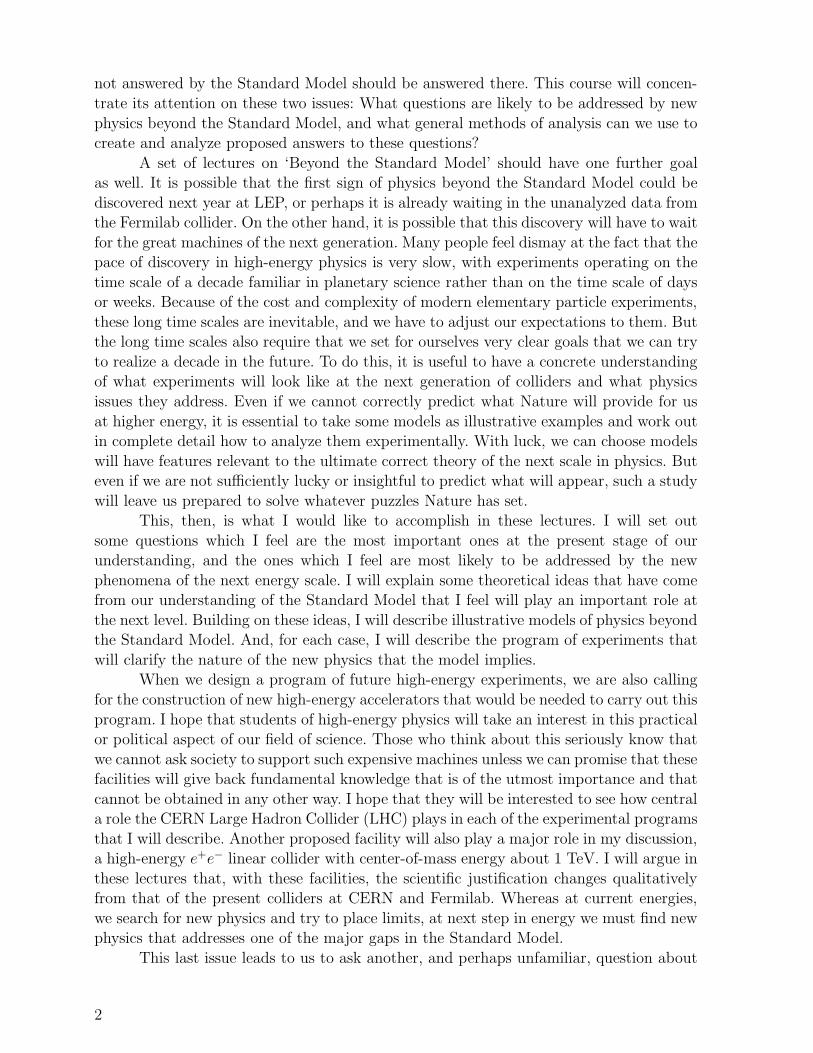
5–97 8303A18
k
+ + +
i jj i jiji
k k k
Figure 2: Diagrams which renormalize the Higgs coupling constant in the Minimal Stan-dard Model.
For massless fermions, there is an ambiguity in writing the quantum numbers in
such a chiral situation becuase a left-handed fermion has a right-handed antifermion, andvice versa. For reasons that will be clearer in the next section, I will choose the convention
of writing all species of fermions in terms of their left-handed components, viewing allright-handed particles as antiparticles. Thus, I will now recast the right-handed u quark in
(24) as the antiparticle of a left-handed species u which belongs to the 3 representation ofcolor SU(3). The fermions of the Standard Model thus belong to the left-handed multiplets
L : I =1
2, Y = −1
2Q : I =
1
2, Y =
1
6
e : I = 0, Y = 1 u : I = 0, Y = −2
3
d : I = 0, Y =1
3. (27)
Here L is the left-handed lepton doublet and Q is the left-handed quark doublet. Q is acolor 3, and u, d are color 3’s. The right-handed electron is the antiparticle of e, and there
is no right-handed neutrino. This set of quantum numbers of repeated for each quark andlepton generation.
If the dimensionless couplings of the theory at TeV energies are small, these cou-
pling will run according to their renormalization group equations, but only at a loga-rithmic rate. Thus, above the TeV scale, the description of elementary particles would
change very slowly. In this circumstance, it is reasonable to extrapolate many orders ofmagnitude above the TeV energy scale and to derive definite physical conclusions from
that extrapolation. I will now describe two consequences of this idea.The first of these concerns the coupling constant of the minimal Higgs theory. For
this analysis, it is best to write the Higgs multiplet as four real-valued fields as in (22).Then the Higgs Lagrangian (ignoring the mass term) takes the form
L =1
2(∂µφ
i)2 − 1
2λb((φi)2
)2, (28)
where i = 1, . . . , 4. I have given the coupling a subscript b to remind us that this is the
bare coupling. The value of the first, tree-level, diagram shown in Figure 2 is
− 2iλb(δijδkℓ + δikδjℓ + δiℓδjk
). (29)
12

To compute the three one-loop diagrams in Figure 2, we need to contract two of these
structures together, using δii = 4 where necessary. The easiest way to do this is to isolate
the terms in each diagram which are proportional to δijδkℓ. Since the set of three diagramsis symmetric under crossing, the other two index contractions must appear also with equal
coefficients. The contributions to this term from the three loop diagrams shown in Figure2 have the form
(−2iλb)2
2
∫d4k
(2π)4
i
k2
i
k2
([8 + 2 + 2]δijδkℓ + · · ·
), (30)
where I have ignored the external momentum, and the numbers in the bracket give the
contribution from each diagram. In a scattering process, this expression is a good approx-imation when k lies in the range from the momentum transfer Q up to the scale Λ at
which the Minimal Standard Model breaks down. Then the sum of the diagrams in Figure2 is
− 2iλb
(1 − 12λ2
b
(4π)2log
Λ2
Q2
)·[δijδkℓ + · · ·
]. (31)
The coefficient in this expression can be thought of as the effective value of the Higgs
coupling constant for scattering processes at the momentum transfer Q. Often, we tradethe bare coupling λb for the value of the effective coupling at a low-energy scale (for
example, v), which we call the renormalized coupling λr. In terms of λr, (31) takes theform
− 2iλr
(1 +
12λ2r
(4π)2log
Q2
v2
)·[δijδkℓ + · · ·
]. (32)
Whichever description we choose, the effective coupling λ(Q) has a logarithmically
slow variation with Q. The most convenient way to describe this variation is by writing a
differential equation, called the renormalization group equation [5]
d
d logQλ(Q) =
3
2π2λ2(Q) . (33)
If the coupling is not so weak, we should add further terms to the right-hand side which
arise from higher orders of perturbation theory.The solution of (33) is
λ(Q) =λr
1 − (3λ/2π2) logQ/v(34)
It is interesting that the effective coupling is predicted to become strong at high energy,specifically, at the scale
Q∗ = v exp
[2π2
3λ
]. (35)
Either the minimal Higgs Lagrangian is a consequence of strong-interaction behavior at
the scale Q∗, or, at some energy scale below Q∗ the simple Higgs theory must become apart of some more complex set of interactions.
Making use of (6), we can relate this bound on the validity of the simple Higgstheory to the value of the Higgs mass, be rewriting (35) as
Q∗ = v exp
[4π2v2
3m2h
]. (36)
13
00
100
100
Q∗ (GeV)
103
106
1010
1015
1019
200mt (GeV)
mH
(G
eV)
300
5–97 8303A01
200
300
400
500
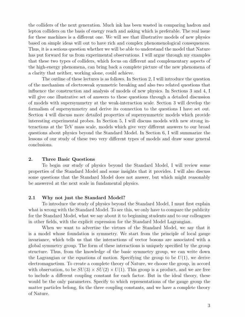
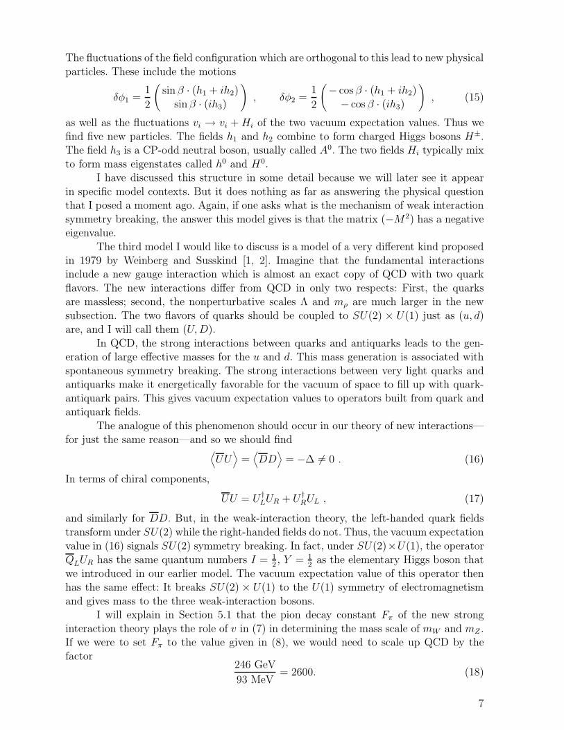
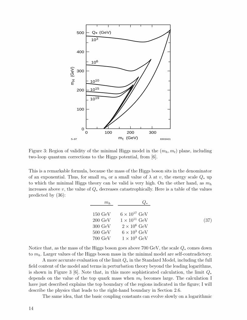
Figure 3: Region of validity of the minimal Higgs model in the (mh, mt) plane, including
two-loop quantum corrections to the Higgs potential, from [6].
This is a remarkable formula, because the mass of the Higgs boson sits in the denominator
of an exponential. Thus, for small mh or a small value of λ at v, the energy scale Q∗ upto which the minimal Higgs theory can be valid is very high. On the other hand, as mh
increases above v, the value of Q∗ decreases catastrophically. Here is a table of the valuespredicted by (36):
mh Q∗
150 GeV 6 × 10¹⁷ GeV200 GeV 1 × 10¹¹ GeV
300 GeV 2 × 10⁶ GeV500 GeV 6 × 10³ GeV
700 GeV 1 × 10³ GeV
(37)
Notice that, as the mass of the Higgs boson goes above 700 GeV, the scale Q∗ comes down
to mh. Larger values of the Higgs boson mass in the minimal model are self-contradictory.
A more accurate evaluation of the limit Q∗ in the Standard Model, including the fullfield content of the model and terms in perturbation theory beyond the leading logarithms,
is shown in Figure 3 [6]. Note that, in this more sophisticated calculation, the limit Q∗depends on the value of the top quark mass when mt becomes large. The calculation I
have just described explains the top boundary of the regions indicated in the figure; I willdescribe the physics that leads to the right-hand boundary in Section 2.6.
The same idea, that the basic coupling constants can evolve slowly on a logarithmic
14
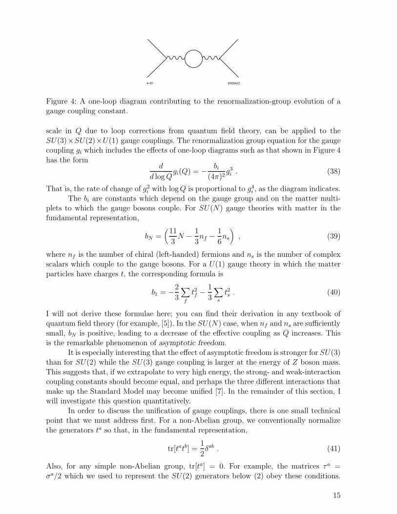
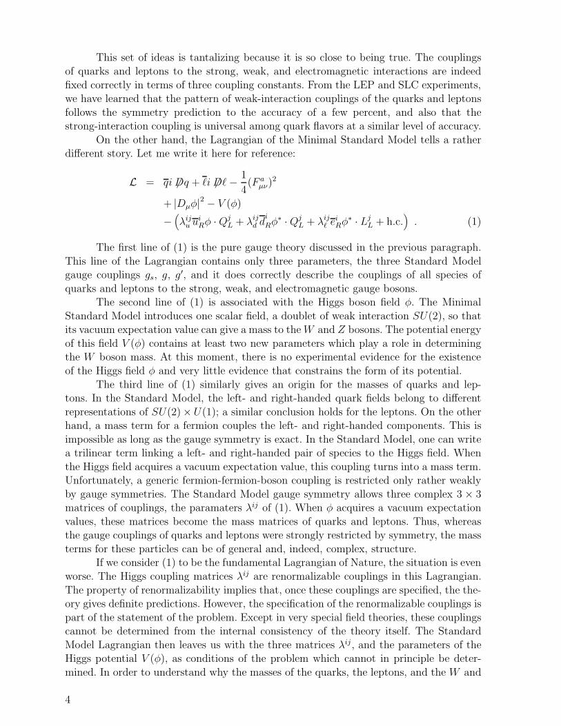
4–97 8303A22
Figure 4: A one-loop diagram contributing to the renormalization-group evolution of agauge coupling constant.
scale in Q due to loop corrections from quantum field theory, can be applied to the
SU(3)×SU(2)×U(1) gauge couplings. The renormalization group equation for the gaugecoupling gi which includes the effects of one-loop diagrams such as that shown in Figure 4
has the formd
d logQgi(Q) = − bi
(4π)2g3i . (38)
That is, the rate of change of g2i with logQ is proportional to g4
i , as the diagram indicates.
The bi are constants which depend on the gauge group and on the matter multi-plets to which the gauge bosons couple. For SU(N) gauge theories with matter in the
fundamental representation,
bN =(
11
3N − 1
3nf −
1
6ns
), (39)
where nf is the number of chiral (left-handed) fermions and ns is the number of complex
scalars which couple to the gauge bosons. For a U(1) gauge theory in which the matter
particles have charges t, the corresponding formula is
b1 = −2
3
∑
f
t2f −1
3
∑
s
t2s . (40)
I will not derive these formulae here; you can find their derivation in any textbook ofquantum field theory (for example, [5]). In the SU(N) case, when nf and ns are sufficiently
small, bN is positive, leading to a decrease of the effective coupling as Q increases. Thisis the remarkable phenomenon of asymptotic freedom.
It is especially interesting that the effect of asymptotic freedom is stronger for SU(3)than for SU(2) while the SU(3) gauge coupling is larger at the energy of Z boson mass.
This suggests that, if we extrapolate to very high energy, the strong- and weak-interactioncoupling constants should become equal, and perhaps the three different interactions that
make up the Standard Model may become unified [7]. In the remainder of this section, Iwill investigate this question quantitatively.
In order to discuss the unification of gauge couplings, there is one small technicalpoint that we must address first. For a non-Abelian group, we conventionally normalize
the generators ta so that, in the fundamental representation,
tr[tatb] =1
2δab . (41)
Also, for any simple non-Abelian group, tr[ta] = 0. For example, the matrices τa =
σa/2 which we used to represent the SU(2) generators below (2) obey these conditions.
15
However, for a U(1) group there is no similar natural way to normalize the charges. In
principle, we could hypothesize that the SU(2) and SU(3) charges are unified with a
charge proportional to the hypercharge,
tY = c · Y (42)
for any value of the scale factor c.
In building a theory of unified strong, weak, and electromagnetic interactions, wemight not want to assume that all fermion species necessarily belong to the fundamental
representation of some SU(N) group; thus, we would not wish to impose the condition(41) on tY . But it is not so unreasonable to insist that there is a single large non-Abelian
group for which tY and the SU(2) and SU(3) charges are all generators, and that thequarks and leptons of the Standard Model form a representation of this group. This leads
to the normalization condition for tY ,
tr(tY )2 = tr(t)2 , (43)
where t is a generator of SU(2) or SU(3). Any such generator gives the same constraint.For convenience, I will choose to implement this condition using t = t3, the third compo-
nent of weak-interaction isospin. The trace could be taken over three or over one StandardModel generations. Before evaluating c, it is interesting to sum over the fermions with
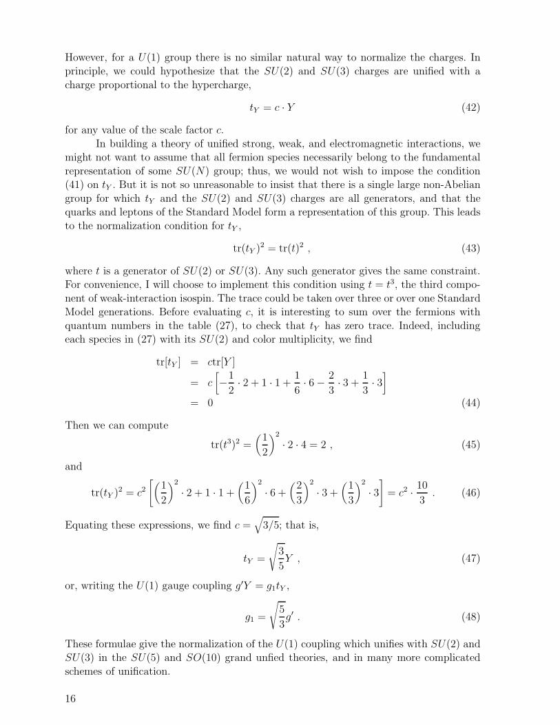
quantum numbers in the table (27), to check that tY has zero trace. Indeed, includingeach species in (27) with its SU(2) and color multiplicity, we find
tr[tY ] = ctr[Y ]
= c[−1
2· 2 + 1 · 1 +
1
6· 6 − 2
3· 3 +
1
3· 3]
= 0 (44)
Then we can compute
tr(t3)2 =(
1
2
)2
· 2 · 4 = 2 , (45)
and
tr(tY )2 = c2[(
1
2
)2
· 2 + 1 · 1 +(
1
6
)2
· 6 +(
2
3
)2
· 3 +(
1
3
)2
· 3]
= c2 · 10
3. (46)
Equating these expressions, we find c =√
3/5; that is,
tY =
√3
5Y , (47)
or, writing the U(1) gauge coupling g′Y = g1tY ,
g1 =
√5
3g′ . (48)
These formulae give the normalization of the U(1) coupling which unifies with SU(2) andSU(3) in the SU(5) and SO(10) grand unfied theories, and in many more complicated
schemes of unification.
16
0
20
40
60
104
Q (GeV)4–97 8303A2
108 1012 1016 1020
α–11
α–1α–1 2
α–13
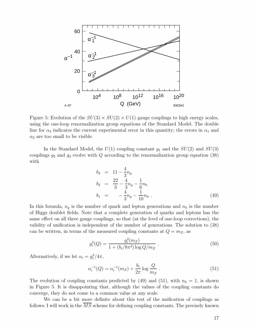
Figure 5: Evolution of the SU(3) × SU(2) × U(1) gauge couplings to high energy scales,
using the one-loop renormalization group equations of the Standard Model. The doubleline for α3 indicates the current experimental error in this quantity; the errors in α1 and
α2 are too small to be visible.
In the Standard Model, the U(1) coupling constant g1 and the SU(2) and SU(3)
couplings g2 and g3 evolve with Q according to the renormalization group equation (38)with
b3 = 11 − 4
3ng
b2 =22
3− 4
3ng −
1
6nh
b1 = − 4
3ng −
1
10nh . (49)
In this formula, ng is the number of quark and lepton generations and nh is the number
of Higgs doublet fields. Note that a complete generation of quarks and leptons has thesame effect on all three gauge couplings, so that (at the level of one-loop corrections), the
validity of unification is independent of the number of generations. The solution to (38)
can be written, in terms of the measured coupling constants at Q = mZ , as
g2i (Q) =
g2i (mZ)
1 + (bi/8π2) logQ/mZ. (50)
Alternatively, if we let αi = g2i /4π,
α−1i (Q) = α−1
i (mZ) +bi2π
logQ
mZ
. (51)
The evolution of coupling constants predicted by (49) and (51), with nh = 1, is shownin Figure 5. It is disappointing that, although the values of the coupling constants do
converge, they do not come to a common value at any scale.We can be a bit more definite about this test of the unification of couplings as
follows: I will work in the MS scheme for defining coupling constants. The precisely known
17
values of α, mZ , and GF imply α−1(mZ) = 127.90± .09, sin2 θw(mZ) = 0.2314± .003 [11];
combining this with the value of the strong interaction coupling αs(mZ) = 0.118 ± .003
[8], we find for the MS couplings at Q = mZ :
α−11 = 58.98 ± .08
α−12 = 29.60 ± .04
α−13 = 8.47 ± .22 (52)
On the other hand, if we assume that the three couplings come to a common value ata scale mU , we can put Q = mU into the three equations (51), eliminate the unknowns
α−1(mU) and log(mU/mZ), and find one relation among the measured coupling constantsat mZ . This relation is
α−13 = (1 +B)α−1
2 − Bα−11 , (53)
where
B =b3 − b2b2 − b1
. (54)
From the data, we find
B = 0.719 ± .008 ± .03 , (55)
where the second error reflects the omission of higher order corrections, that is, finite
radiative corrections at the thresholds and two-loop corrections in the renormalizationgroup equations.
On the other hand, the Standard Model gives
B =1
2+
3
110nh . (56)
This is inconsistent with the unification hypothesis by a large margin. But perhaps an
interesting scheme for physics beyond the Standard Model could fill this gap and allow aunification of the known gauge couplings.
2.6 The special role of the top quark
In the previous section, we discussed the role of the quarks and leptons in theenergy region above 1 TeV. However, we ought to give additional consideration to the
role of the top quark. This quark is sufficiently heavy that its coupling to the Higgsboson is an important perturbative coupling at very high energies. Thus, even in the
simplest models, the top quark plays an important special role in the renormalizationgroup evolution of couplings. It is possible that the top quark has an even more central
role in electroweak symmetry breaking, and, in fact, that electroweak symmetry breaking
may be caused by the strong interactions of the top quark. I will discuss this connection ofthe top quark to electroweak symmetry breaking later, in the context of specific models.
In this section, I would like to prepare for that discussion by analyzing the effects of thelarge top quark-Higgs boson coupling which is already present in the Minimal Standard
Model.In the minimal Higgs model, the masses of quarks and leptons arise from the
perturbative couplings to the Higgs boson written in the third line of (1). These couplings
18
are most often called the ‘Higgs Yukawa couplings’. The top quark mass comes from a
Yukawa coupling
∆L = −λttRφ ·QL + h.c. , (57)
where QL = (tL, bL). When the Higgs field acquires a vacuum expectation value of the
form (4), this term becomes
∆L = −λtv√2tt, (58)
and we can read off the relation mt = λtv/√
2. The value of the top quark mass measuredat Fermilab is 176 ± 6 GeV for the on-shell mass [9], which corresponds to
(mt)MS = 166 ± 6 GeV . (59)
With the value of v in (8), this implies
λt = 1 or αt =λ2
4π= (14.0 ± 0.7)−1 . (60)
In this simplest model, the top quark Yukawa coupling is weak at high energies but still
is large enough to compete with QCD.The large value of λt gives rise to two interesting effects. The first of these is an
essential modification of the renormalization group equation for the Higgs boson couplingλ given in (33). Let me now rewrite this equation including the one-loop corrections due
to λt and also to the weak-interaction couplings [10]:
d
d logQλ =
3
2π2
[λ2 − 1
32λ4t +
g2
512(3 + 2s2 + s4)
], (61)
where I have abbreviated s2 = sin2 θw.
A remarkable property of the formula (61) is that the top quark Yukawa coupling
enters the renormalization group equation with a negative sign (which essentially comesfrom the factor (-1) for the top quark fermion loop). This sign implies that, if the top
quark mass is sufficiently large that that λ4 term dominates, the Higgs coupling λ is drivennegative at largeQ. This is a dangerous instability which would push the expectation value
v of the Higgs field to arbitrarily high values. The presence of this instability gives anupper bound on the top quark mass for fixed mh, or, equivalently, a lower bound on the
Higgs mass for fixed mt. If we replace λ, λt, and g in (61) with the masses of h, t, andW , we find the condition
m2h >
1
2
[m2t −
3
4m2W
]. (62)
I should note that finite perturbative corrections shift this bound in a way that is impor-
tant quantitatively. This effect accounts for the right-hand boundary of the regions shownin Figure 3.
The implications of Figure 3 for the Higgs boson mass are quite interesting. Forthe correct value of the top quark mass (59), the Minimal Standard Model description of
the Higgs boson can be valid only if the mass of the Higgs is larger than about 60 GeV.But for values of the mh below 100 GeV or above 200 GeV, the Higgs coupling must be
sufficiently large that this coupling becomes strong well below the Planck scale. Curiously,
19
the fit of current precision electroweak data to the Minimal Standard Model (for example,
to the more precise version of (23)) gives the value [11]
mh = 124+125−71 GeV , (63)
which actually lies in the region for which the Minimal Standard Model is good to ex-
tremely high energies. It is also important to point out that the regions of Figure 3 apply
only to the Minimal version of the Standard Model. In models with additional Higgs dou-blets, with the boundaries giving limits on the lightest Higgs boson, the upper boundary
remains qualitatively correct, but the boundary associated with the heavy top quark isusually pushed far to the right.
The second perturbative effect of the top quark Yukawa coupling is its influenceback on its own renormalization group evolution. In the same simple one-loop approxi-
mation as (61), the renormalization group equation for the top quark Yukawa couplingtakes the form
d
d logQλt =
λt(4π)2
[9
2λ2t − 8g2
3 −9
4g2(1 +
17
24s2)]
. (64)
The signs in this equation are not hard to understand. A theory with λt and no gauge
couplings cannot be asymptotically free, and so λt must drive itself to zero at largedistances or small Q. On the other hand, the effect of the QCD coupling g3 is to increase
quark masses and also λt as Q becomes small.The two effects of the λt and QCD renormalization of λt balance at the point
λt =4
3(4παs)
1/2 ∼ 1.5 , (65)
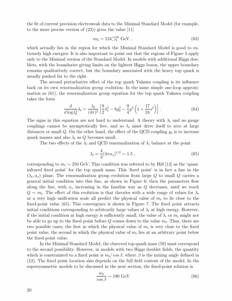
corresponding to mt ∼ 250 GeV. This condition was referred to by Hill [12] as the ‘quasi-
infrared fixed point’ for the top quark mass. This ‘fixed point’ is in fact a line in the
(λt, αs) plane. The renormalization group evolution from large Q to small Q carries ageneral initial condition into this line, as shown in Figure 6; then the parameters flow
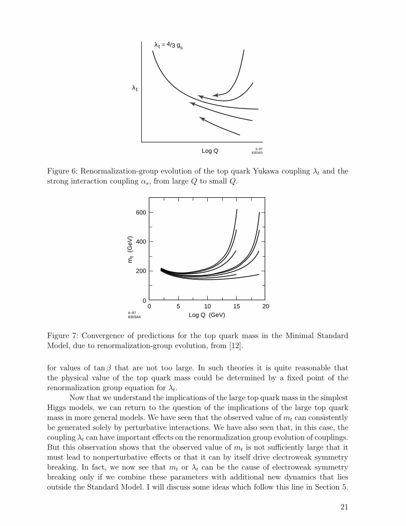
along the line, with αs increasing in the familiar way as Q decreases, until we reachQ ∼ mt. The effect of this evolution is that theories with a wide range of values for λtat a very high unification scale all predict the physical value of mt to lie close to thefixed-point value (65). This convergence is shown in Figure 7. The fixed point attracts
initial conditions corresponding to arbitrarily large values of λt at high energy. However,if the initial condition at high energy is sufficiently small, the value of λt or mt might not
be able to go up to the fixed point before Q comes down to the value mt. Thus, there aretwo possible cases, the first in which the physical value of mt is very close to the fixed
point value, the second in which the physical value of mt lies at an arbitrary point belowthe fixed-point value.
In the Minimal Standard Model, the observed top quark mass (59) must correspondto the second possibility. However, in models with two Higgs doublet fields, the quantity
which is constrainted to a fixed point is mt/ cosβ, where β is the mixing angle defined in
(12). The fixed point location also depends on the full field content of the model. In thesupersymmetric models to be discussed in the next section, the fixed-point relation is
mt
cosβ∼ 190 GeV (66)
20
Log Q
λ t = 4/3 gs
λ t
5–97 8303A3
Figure 6: Renormalization-group evolution of the top quark Yukawa coupling λt and the
strong interaction coupling αs, from large Q to small Q.
00
200
5Log Q (GeV)
mt
(GeV
)
4–978303A4
10 15 20
400
600
Figure 7: Convergence of predictions for the top quark mass in the Minimal Standard
Model, due to renormalization-group evolution, from [12].
for values of tanβ that are not too large. In such theories it is quite reasonable that
the physical value of the top quark mass could be determined by a fixed point of therenormalization group equation for λt.
Now that we understand the implications of the large top quark mass in the simplestHiggs models, we can return to the question of the implications of the large top quark
mass in more general models. We have seen that the observed value of mt can consistently
be generated solely by perturbative interactions. We have also seen that, in this case, thecoupling λt can have important effects on the renormalization group evolution of couplings.
But this observation shows that the observed value of mt is not sufficiently large that itmust lead to nonperturbative effects or that it can by itself drive electroweak symmetry
breaking. In fact, we now see that mt or λt can be the cause of electroweak symmetrybreaking only if we combine these parameters with additional new dynamics that lies
outside the Standard Model. I will discuss some ideas which follow this line in Section 5.
21
2.7 Recapitulation
In this section, I have introduced the major questions for physics beyond the Stan-
dard Model by reviewing issues that arise when the Standard Model is extrapolated tovery high energy. I have highlighted the issue of electroweak symmetry breaking, which
poses an important question for the Standard Model which must be solved at energiesclose to those of our current accelerators. There are many possibilities, however, for the
form of this solution. The new physics responsible for electroweak symmetry breaking
might be a new set of strong interactions which changes the laws of particle physics fun-damentally at some nearby energy scale. But the analysis we have done tells us that the
solution might be constructed in a completely different way, in which the new interactionsare weakly coupled for many orders of magnitude above the weak interaction scale but
undergoes qualitative changes through the renormalization group evolution of couplings.The questions we have asked in Section 2.4 and this dichotomy of strong-coupling
versus weak-coupling solutions to these questions provide a framework for examiningtheories of physics beyond the Standard Model. In the next sections, I will consider some
explicit examples of such models, and we can see how they illustrate the different possibleanswers.
3. Supersymmetry: Formalism
The first class of models that I would like to discuss are supersymmetric extensionsof the Standard Model. Supersymmetry is defined to be a symmetry of Nature that links
bosons and fermions. As we will see later in this section, the introduction of supersymme-try into Nature requires a profound generalization of our fundamental theories, including
a revision of the theory of gravity and a rethinking of our basic notions of space-time.
For many theorists, the beauty of this new geometrical theory is enough to make it com-pelling. For myself, I think this is quite a reasonable attitude. However, I do not expect
you to share this attitude in order to appreciate my discussion.For the skeptical experimenter, there are other reasons to study supersymmetry.
The most important is that supersymmetry is a concrete worked example of physicsbeyond the Standard Model. One of the virtues of extending the Standard Model using
supersymmetry is that the phenomena that we hope to discover at the next energy scale—the new spectrum of particles, and the mechanism of electroweak symmetry breaking—
occur in supersymmetric models at the level of perturbation theory, without the needfor any new strong interactions. Supersymmetry naturally predicts are large and complex
spectrum of new particles. These particles have signatures which are interesting, andwhich test the capabilities of experiments. Because the theory has weak couplings, these
signatures can be worked out directly in a rather straightforward way. On the otherhand, supersymmetric models have a large number of undetermined parameters, so they
can exhibit an interesting variety of physical effects. Thus, the study of supersymmetric
models can give you very specific pictures of what it will be like to experiment on physicsbeyond the Standard Model and, through this, should aid you in preparing for these
experiments. For this reason, I will devote a large segment of these lectures to a detaileddiscussion of supersymmetry. However, as a necessary corrective, I will devote Section
5 of this article to a review of a model of electroweak symmetry breaking that runs bystrong-coupling effects.
This discussion immediately raises a question: Why is supersymmetry relevant to
22
the major issue that we are focusing on in these lectures, that of the mechanism of elec-
troweak symmetry breaking? A quick answer to this question is that supersymmetry legit-
imizes the introduction of Higgs scalar fields, because it connects spin-0 and spin-12
fieldsand thus puts the Higgs scalars and the quarks and leptons on the same epistemological
footing. A better answer to this question is that supersymmetry naturally gives rise to amechanism of electroweak symmetry breaking associated with the heavy top quark, and to
many other properties that are attractive features of the fundamental interactions. Theseconsequences of the theory arise from renormalization group evolution, by arguments sim-
ilar to those we used to explain the features of the Standard Model that we derived inSections 2.5 and 2.6. The spectrum of new particles predicted by supersymmetry will also
be shaped strongly by renormalization-group effects.In order to explain these effects, I must unfortunately subject you to a certain
amount of theoretical formalism. I will therefore devote this section to describing construc-tion of supersymmetric Lagrangians and the analysis of their couplings. I will conclude
this discussion in Section 3.7 by explaining the supersymmetric mechanism of electroweaksymmetry breaking. This analysis will be lengthy, but it will give us the tools we need to
build a theory of the mass spectrum of supersymmetric particles. With this understanding,
we will be ready in Section 4 to discuss the experimental issues raised by supersymmetry,and the specific experiments that should resolve them.
3.1 A little about fermions
In order to write Lagrangians which are symmetric between boson and fermionfields, we must first understand the properties of these fields separately. Bosons are simple,
one component objects. But for fermions, I would like to emphasize a few features which
are not part of the standard presentation of the Dirac equation.The Lagrangian of a massive Dirac field is
L = ψi 6∂ψ −mψψ , (67)
where ψ is a 4-component complex field, the Dirac spinor. I would like to write thisequation more explicitly by introducing a particular representation of the Dirac matrices
γµ =
(0 σµ
σµ 0
), (68)
where the entries are 2 × 2 matrices with
σµ = (1, ~σ) , σµ = (1,−~σ) . (69)
We may then write ψ as a pair of 2-component complex fields
ψ =
(ψLψR
). (70)
The subscripts indicate left- and right-handed fermion components, and this is justifiedbecause, in this representation,
γ5 =
(−1 0
0 1
). (71)
23
This is a handy representation for calculations involving high-energy fermions which in-
clude chiral interactions or polarization effects, even within the Standard Model [5].
In the notation of (68), (70), the Lagrangian (67) takes the form
L = ψ†Liσ
µ∂µψL + ψ†Riσ
µ∂µψR −m(ψ†RψL + ψ†
LψR). (72)
The kinetic energy terms do not couple ψL and ψR but rather treat them as distinctspecies. The mass term is precisely the coupling between these components.
I pointed out above (27) that, since the antiparticle of a masssless left-handedparticle is a right-handed particle, there is an ambiguity in assigning quantum numbers
to fermions. I chose to resolve this ambiguity by considering all left-handed states asparticles and all right-handed states as antiparticles. With this philosophy, we would like
to trade ψR for a left-handed field. To do this, define the 2 × 2 matrix
c = −iσ2 =
(0 −1
1 0
). (73)
and let
χL = cψ∗R , χ∗
L = cψR (74)
Note that c−1 = cT = −c, c∗ = c, so (74) implies
ψR = −cχ∗L , ψ†
R = χTLc . (75)
Also note, by multiplying out the matrices, that
cσµc−1 = (σµ)T , cσµc−1 = (σµ)T . (76)
Using these relations, we can rewrite
ψ†Riσ
µ∂µψR = χTLciσµ∂µ(−c)χ∗
L
= χTLi(σµ)T∂µχ
∗L
= −∂µχ†Li(σ
µ)χL
= χ†Liσ
µ∂µχL . (77)
The minus sign in the third line came from fermion interchange; it was eliminated in thefourth line by an integration by parts. After this rewriting, the two pieces of the Dirac
kinetic energy term have precisely the same form, and we may consider ψL and χL as twospecies of the same type of particle.
If we replace ψR by χL, the mass term in (67) becomes
−m(ψ†RψL + ψ†
LψR)
= −m(χTLcψL − ψ†
Lcχ∗L
). (78)
Note that
χTLcψL = ψTLcχL , (79)
with one minus sign from fermion interchange and a second from taking the transpose of
c. Thus, this mass term is symmetric between the two species. It is interesting to know
24
that the most general possible mass term for spin-12
fermions can be written in terms of
left-handed fields ψaL in the form
− 1
2mabψaTL cψbL + h.c. , (80)
where mab is a symmetric matrix. For example, this form for the mass term incorporates
all possible different forms of the neutrino mass matrix, both Dirac and Majorana.From here on, through the end of Section 4, all of the fermions that appear in these
lectures will be 2-component left-handed fermion fields. For this reason, there will be noambiguity if I now drop the subscript L in my equations.
3.2 Supersymmetry transformations
Now that we have a clearer understanding of fermion fields, I would like to explore
the possible symmetries that could connect fermions to bosons. To begin, let us try toconnect a free massless fermion field to a free massless boson field. Because the scalar
product (79) of two chiral fermion fields is complex, this connection will not work unlesswe take the boson field to be complex-valued. Thus, we should look for symmetries of the
LagrangianL = ∂µφ
∗∂µφ+ ψ†iσ · ∂ψ (81)
which mix φ and ψ.To build this transformation, we must introduce a symmetry parameter with spin-1
2
to combine with the spinor index of ψ. I will introduce a parameter ξ which also transformsas a left-handed chiral spinor. Then a reasonable transformation law for φ is
δξφ =√
2ξT cψ . (82)
A fermion field has the dimensions of (mass)3/2, while a boson field has the dimensions of
(mass)1; thus, xi must carry the dimensions (mass)−1/2 or (length)1/2. This means that,in order to form a dimensionally correct transformation law for ψ, we must include a
derivative. A sensible formula is
δξψ =√
2iσ · ∂φcξ∗ . (83)
It is not difficult to show that the transformation (82), (83) is a symmetry of (81).Inserting these transformations, we find
δξL = ∂µφ∗∂µ(
√2ξT cψ) + (
√2iξT cσ · ∂φ)iσ · ∂ψ + (ξ∗) . (84)
The term in the first set of parentheses is the right-hand side of (82). The term in the
second set of parentheses is the Hermitian conjugate of the right-hand side of (83). Thelast term refers to terms proportional to ξ∗ arising from the variation of φ∗ and ψ. To
manipulate (84), integrate both terms by parts and use the identity
σ · ∂σ · ∂ = ∂2 (85)
which can be verified directly from (69). This gives
δξL = −φ∗∂2(√
2ξT cψ) −√
2iξT c · i∂2ψ + (ξ∗) . (86)
25
The two terms shown now cancel, and the ξ∗ terms cancel similarly. Thus, δξL = 0 and
we have a symmetry.
The transformation (83) appears rather strange at first sight. However, this formulatakes on a bit more sense when we work out the algebra of supersymmetry transformations.
Consider the commutator
(δηδξ − δξδη)φ = δη(√
2ξT cψ) − (η ↔ ξ)
=√
2ξT c(√
2iσµ∂µφcη∗) − (η ↔ ξ)
= 2iξT cσµcη∗∂µφ− (η ↔ ξ)
= −2iξT (σµ)Tη∗∂µφ− (η ↔ ξ)
= 2i[η†σµξ − ξ†σµη] ∂µφ . (87)
To obtain the fourth line, I have used (76); in the passage to the next line, a minus signappears due to fermion interchange. In general, supersymmetry transformations have the
commutation relation
(δηδξ − δξδη)A = 2i[η†σµξ − ξ†σµη] ∂µA (88)
on every field A of the theory.To clarify the significance of this commutation relation, let me rewrite the trans-
formations δξ as the action of a set of operators, the supersymmetry charges Q. Thesecharges must also be spin-1
2. To generate the supersymmetry transformation, we contract
them with the spinor parameter ξ; thus
δξ = ξT cQ−Q†cξ∗ . (89)
At the same time, we may replace (i∂µ) in (88) by the operator which generates spa-
tial translations, the energy-momentum four-vector P µ. Then (88) becomes the operatorrelation {
Q†a , Qb
}= (σµ)abPµ (90)
which defines the supersymmetry algebra. This anticommutation relation has a two-foldinterpretation. First, it says that the square of the supersymmetry charge Q is the energy-
momentum. Second, it says that the square of a supersymmetry transformation is a spatialtranslation. The idea of a square appears here in the same sense as we use when we say
that the Dirac equation is the square root of the Klein-Gordon equation.We started this discussion by looking for symmetries of the trivial theory (81), but
at this stage we have encountered a structure with deep connections. So it is worth lookingback to see whether we were forced to come to high level or whether we could have taken
another route. It turns out that, given our premises, we could not have ended in any otherplace [13]. We set out to look for an operator Q that was a symmetry of Nature which
carried spin-12. From this property, the quantity on the left-hand side of (90) is a Lorentz
four-vector which commutes with the Hamiltonian. In principle, we could have written a
more general formula {Q†a , Qb
}= (σµ)abRµ , (91)
where Rµ is a conserved four-vector charge different from P µ. But energy-momentum
conservation is already a very strong restriction on particle scattering processes, since
26
it implies that the only degree of freedom in a two-particle reaction is the scattering
angle in the center-of-mass system. A second vector conservation law, to the extent that
it differs from energy-momentum conservation, places new requirements that contradictthese restrictions except at particular, discrete scattering angles. Thus, it is not possible
to have an interacting relativistic field theory with an additional conserved spin-1 charge,or with any higher-spin charge, beyond standard momentum and angular momentum
conservation [14]. For this reason, (90) is actually the most general commutation relationthat can be obeyed by supersymmetry charges.
The implications of the supersymmetry algebra (90) are indeed profound. If thesquare of a supersymmetry charge is the total energy-momentum of everything, then
supersymmetry must act on every particle and field in Nature. We can exhibit this actionexplicitly by writing out the a = 1, b = 1 component of (90),
{Q†
1 , Q1
}= P 0 + P 3 = P+ . (92)
On states with P+ 6= 0 (which we can arrange for any particle state by a rotation), define
a =Q1√P+
, a† =Q†
1√P+
. (93)
These operators obey the algebra{a† , a} = 1 (94)
of fermion raising and lowering operators. They raise and lower J3 by 12
unit. Thus, in asupersymmetric theory, every state of nonzero energy has a partner of opposite statistics
differing in angular momentum by ∆J3 = ±12.
On the other hand, for any operator Q, the quantity {Q†, Q} is a Hermitian matrix
with eigenvalues that are either positive or zero. This matrix has zero eigenvalues for thosestates that satisfy
Q |0〉 = Q† |0〉 = 0 , (95)
that is, for supersymmetric states. In particular, if supersymmetry is not spontaneously
broken, the vacuum state is supersymmetric and satisfies (95). Since the vacuum also haszero three-momentum, we deduce
〈0|H |0〉 = 0 (96)
as a consequence of supersymmetry. Typically in a quantum field theory, the value of the
vacuum energy density is given by a complicated sum of vacuum diagrams. In a super-symmetric theory, these diagrams must magically cancel [15]. This is the first of a number
of magical cancellations of radiative corrections that we will find in supersymmetric fieldtheories.
3.3 Supersymmetric Lagrangians
At this point, we have determined the general formal properties of supersymmet-
ric field theories. Now it is time to be much more concrete about the form of the La-
grangians which respect supersymmetry. In this section, I will discuss the particle contentof supersymmetric theories and present the most general renormalizable supersymmetric
Lagrangians for spin-0 and spin-12
fields.
27
We argued from (92) that all supersymmetric states of nonzero energy are paired. In
particular, this applies to single-particle states, and it implies that supersymmetric models
contain boson and fermion fields which are paired in such a way that the particle degreesof freedom are in one-to-one correspondence. In the simple example (81), I introduced a
complex scalar field and a left-handed fermion field. Each leads to two sets of single-particlestates, the particle and the antiparticle. I will refer to this set of states—a left-handed
fermion, its right-handed antiparticle, a complex boson, and its conjugate—as a chiral
supermultiplet.
Another possible pairing is a a massless vector field and a left-handed fermion,which gives a vector supermultiplet—two transversely polarized vector boson states, plus
the left-handed fermion and its antiparticle. In conventional field theory, a vector bosonobtains mass from the Higgs mechanism by absorbing one degree of freedom from a scalar
field. In supersymmetry, the Higgs mechanism works by coupling a vector supermultipletto a chiral supermultiplet. This coupling results in a massive vector particle, with three
polarization states, plus an extra scalar. At the same time, the left-handed fermions inthe two multiplets combine through a mass term of the form (78) to give a massive Dirac
fermion, with two particle and two antiparticle states. All eight states are degenerate if
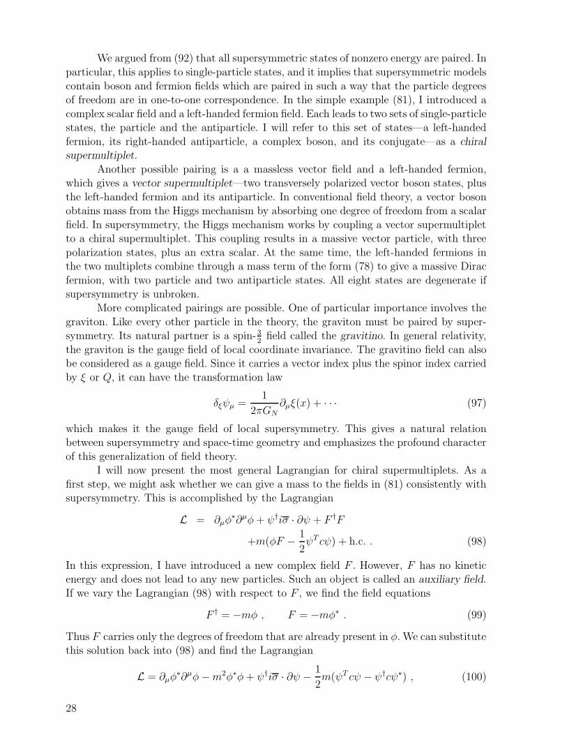
supersymmetry is unbroken.More complicated pairings are possible. One of particular importance involves the
graviton. Like every other particle in the theory, the graviton must be paired by super-symmetry. Its natural partner is a spin-3
2field called the gravitino. In general relativity,
the graviton is the gauge field of local coordinate invariance. The gravitino field can alsobe considered as a gauge field. Since it carries a vector index plus the spinor index carried
by ξ or Q, it can have the transformation law
δξψµ =1
2πGN∂µξ(x) + · · · (97)
which makes it the gauge field of local supersymmetry. This gives a natural relationbetween supersymmetry and space-time geometry and emphasizes the profound character
of this generalization of field theory.I will now present the most general Lagrangian for chiral supermultiplets. As a
first step, we might ask whether we can give a mass to the fields in (81) consistently withsupersymmetry. This is accomplished by the Lagrangian
L = ∂µφ∗∂µφ+ ψ†iσ · ∂ψ + F †F
+m(φF − 1
2ψT cψ) + h.c. . (98)
In this expression, I have introduced a new complex field F . However, F has no kineticenergy and does not lead to any new particles. Such an object is called an auxiliary field.
If we vary the Lagrangian (98) with respect to F , we find the field equations
F † = −mφ , F = −mφ∗ . (99)
Thus F carries only the degrees of freedom that are already present in φ. We can substitutethis solution back into (98) and find the Lagrangian
L = ∂µφ∗∂µφ−m2φ∗φ+ ψ†iσ · ∂ψ − 1
2m(ψT cψ − ψ†cψ∗) , (100)
28
which has equal, supersymmetric masses for the bosons and fermions.
It is not difficult to show that the Lagrangian (98) is invariant to the supersymmetry
transformation
δξφ =√
2ξT cψ
δξψ =√
2iσ · ∂φcξ∗ + ξF
δξF = −√
2iξ†σ · ∂ψ . (101)
The two lines of (98) are invariant separately. For the first line, the proof of invariance isa straightforward generalization of (86). For the second line, we need
δξ(φF − 1
2ψT cψ) = (
√2ξT cψ)F + φ(−
√2iξ†σ · ∂ψ) − ψT c(
√2iσ · ∂φcξ∗ + ξF )
=√
2iξ†σ · ∂ψ −√
2iψT cσ · ∂φcξ∗
= 0 . (102)
The first and last terms in the second line cancel by the use of (79); the terms in the third
line cancel after an integration by parts and a rearrangement similar to that in (87) in thesecond term. Thus, (101) is an invariance of (98). With some effort, one can show that
this transformation obeys the supersymmetry algebra, in the sense that the commutatorsof transformations acting on φ, ψ, and F follow precisely the relation (88).
The introduction of the auxiliary field F allows us to write a much more generalclass of supersymmetric Lagrangians. Let φj, ψj , Fj be the fields of a number of chiral
supermultiplets indexed by j. Assign each multiplet the supersymmetry transformationlaws (101). Then it can be shown by a simple generalization of the discussion just given
that the supersymmetry transformation leaves invariant Lagrangians of the general form
L = ∂µφ∗j∂
µφj + ψ†j iσ · ∂ψj + F †
j Fj
+(Fj∂W
∂φj− 1
2ψTj cψk
∂2W
∂φj∂φk) + h.c. , (103)
where W (φ) is an analytic function of the complex fields φj which is called the superpo-
tential. It is important to repeat that W (φ) can have arbitrary dependence on the φj , butit must not depend on the φ∗
j . The auxiliary fields Fj obey the equations
F † = −∂W∂φj
. (104)
If W is a polynomial in the φj , the elimination of the Fj by substituting (104) into (103)
produces polynomial interactions for the scalar fields.The free massive Lagrangian (98) is a special case of (103) for one supermultiplet
with the superpotential
W =1
2mφ2 . (105)
A more interesting model is obtained by setting
W =1
3λφ3 . (106)
29
+
(a)
4–97 8303A16
ψ
ψ
φ
φ φ
φ φ
(b)
Figure 8: (a) Yukawa and four-scalar couplings arising from the supersymmetric La-grangian with superpotential (106); (b) Diagrams which give the leading radiative correc-
tions to the scalar field mass term.
In this case, W leads directly to a Yukawa coupling proportional to λ, while substitutingfor F from (104) yields a four scalar coupling proportional to λ2:
L = ∂µφ∗∂µφ+ ψ†iσ · ∂ψ − λ2|φ2|2 − λ[ψT cψφ− φ∗ψ†cψ∗] . (107)
These two vertices are shown in Figure 8(a). Their sizes are such that the two leadingdiagrams which contribute to the scalar field mass renormalization, shown in Figure 8(b),
are of the same order of magnitude. In fact, it is not difficult to compute these diagramsfor external momentum p = 0. The first diagram has the value
− 4λ2i ·∫
d4k
(2π)4
i
k2= 4λ2
∫d4k
(2π)4
1
k2. (108)
To compute the second diagram, note that the standard form of the fermion propagator is⟨ψψ†
⟩, and be careful to include all minus signs resulting from fermion reordering. Then
you will find
1
2(−2iλ)(2iλ)
∫d4k
(2π)4tr
[iσ · kk2
c(−iσ · kk2
)T c
]
= −2λ2∫
d4k
(2π)4
tr[σ · kσ · k]k4
. (109)
Using (85), the trace gives 2k2, and the two diagrams cancel precisely. Thus, the choice
(106) presents us with an interacting quantum field theory, but one with exceptional
cancellations in the scalar field mass term.In this simple model, it is not difficult to see that the scalar field mass corrections
must vanish as a matter of principle. The theory with superpotential (106) is invariantunder the symmetry
φ→ e2iαφ , ψ → e−iαψ . (110)
This symmetry is inconsistent with the appearance of a fermion mass term mψT cψ, as
in (100). The symmetry does not prohibit the appearance of a scalar mass term, but if
30
the theory is to remain supersymmetric, the scalar cannot have a different mass from the
fermion. However, the cancellation of radiative corrections in models of the form (103)
is actually much more profound. It can be shown that, in a general model of this type,the only nonvanishing radiative corrections to the potential terms are field rescalings. If
a particular coupling—the mass term, a cubic interaction, or any other—is omitted fromthe original superpotential, it cannot be generated by radiative corrections [16, 17].
For later reference, I will write the potential energy associated with the most generalsystem with a Lagrangian of the form (103). This is
V = −F †j Fj − Fj
∂W
∂φj− F †
j
(∂W
∂φj
)∗
. (111)
Substituting for Fj from (104), we find
V =∑
j
∣∣∣∣∣∂W
∂φj
∣∣∣∣∣
2
. (112)
This simple result is called the F-term potential. It is minimized by setting all of the Fjequal to zero. If this is possible, we obtain a vacuum state with 〈H〉 = 0 which is also
invariant to supersymmetry, in accord with the discussion of (96). On the other hand,supersymmetry is spontaneously broken if for some reason it is not possible to satisfy all
of the conditions Fj = 0 simultaneously. In that case, we obtain a vacuum state with〈H〉 > 0.
3.4 Coupling constant unification
At this point, we have not yet completed our discussion of the structure of su-persymmetric Lagrangians. In particular, we have not yet written the supersymmetric
Lagrangians of vector fields, beyond simply noting that a vector field combines with achiral fermion to form a vector supermultiplet. Nevertheless, it is not too soon to try to
write a supersymmetric generalization of the Standard Model.I will first list the ingredients needed for this generalization. For each of the SU(3)×
SU(2)×U(1) gauge bosons, we need a chiral fermion λa to form a vector supermultiplet.These new fermions are called gauginos. I will refer the specific partners of specific gauge
bosons with a tilde. For example, the fermionic partner of the gluon will be called g, thegluino, and the fermionic partners of the W+ will be called w+, the wino.
None of these fermions have the quantum numbers of quarks and leptons. So weneed to add a complex scalar for each chiral fermion species to put the quarks and leptons
into chiral supermultiplets. I will use the labels for left-handed fermion multiplets in(27) also to denote the quark and lepton supermultiplets. Hopefully, it will be clear from
context whether I am talking about the supermultiplet or the fermion. The scalar partners
of quarks and leptons are called squarks and sleptons. I will denote these with a tilde.For example, the partner of e−L = L− is the selectron e−L or L−. The partner of e∗ = e−Ris a distinct selectron which I will call e−R. The Higgs fields must also belong to chiralsupermultiplets. I will denote the scalar components as hi and the left-handed fermions
as hi. We will see in a moment that at least two different Higgs multiplets are required.Although we need a bit more formalism to write the supersymmetric generalization
of the Standard Model gauge couplings, it is already completely straightforward to write
31
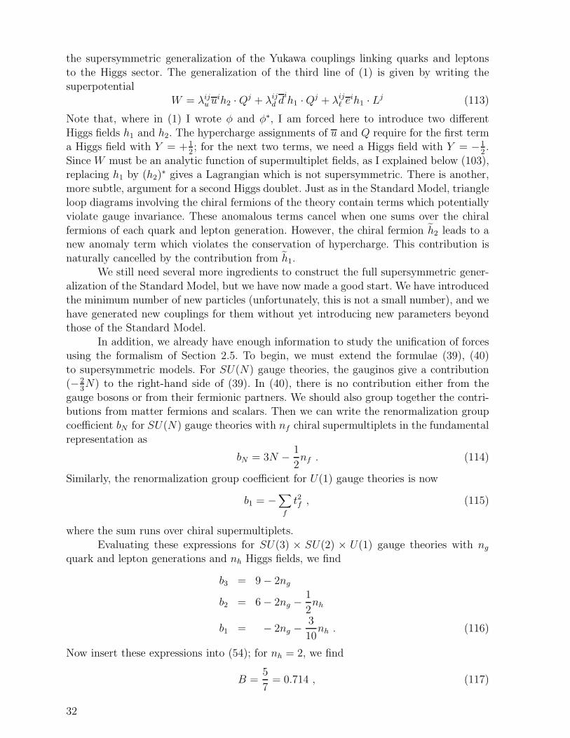
the supersymmetric generalization of the Yukawa couplings linking quarks and leptons
to the Higgs sector. The generalization of the third line of (1) is given by writing the
superpotentialW = λiju u
ih2 ·Qj + λijd dih1 ·Qj + λijℓ e
ih1 · Lj (113)
Note that, where in (1) I wrote φ and φ∗, I am forced here to introduce two different
Higgs fields h1 and h2. The hypercharge assignments of u and Q require for the first terma Higgs field with Y = +1
2; for the next two terms, we need a Higgs field with Y = −1
2.
Since W must be an analytic function of supermultiplet fields, as I explained below (103),replacing h1 by (h2)
∗ gives a Lagrangian which is not supersymmetric. There is another,
more subtle, argument for a second Higgs doublet. Just as in the Standard Model, triangleloop diagrams involving the chiral fermions of the theory contain terms which potentially
violate gauge invariance. These anomalous terms cancel when one sums over the chiral
fermions of each quark and lepton generation. However, the chiral fermion h2 leads to anew anomaly term which violates the conservation of hypercharge. This contribution is
naturally cancelled by the contribution from h1.We still need several more ingredients to construct the full supersymmetric gener-
alization of the Standard Model, but we have now made a good start. We have introducedthe minimum number of new particles (unfortunately, this is not a small number), and we
have generated new couplings for them without yet introducing new parameters beyondthose of the Standard Model.
In addition, we already have enough information to study the unification of forcesusing the formalism of Section 2.5. To begin, we must extend the formulae (39), (40)
to supersymmetric models. For SU(N) gauge theories, the gauginos give a contribution(−2
3N) to the right-hand side of (39). In (40), there is no contribution either from the
gauge bosons or from their fermionic partners. We should also group together the contri-butions from matter fermions and scalars. Then we can write the renormalization group
coefficient bN for SU(N) gauge theories with nf chiral supermultiplets in the fundamental
representation as
bN = 3N − 1
2nf . (114)
Similarly, the renormalization group coefficient for U(1) gauge theories is now
b1 = −∑
f
t2f , (115)
where the sum runs over chiral supermultiplets.
Evaluating these expressions for SU(3) × SU(2) × U(1) gauge theories with ngquark and lepton generations and nh Higgs fields, we find
b3 = 9 − 2ng
b2 = 6 − 2ng −1
2nh
b1 = − 2ng −3
10nh . (116)
Now insert these expressions into (54); for nh = 2, we find
B =5
7= 0.714 , (117)
32
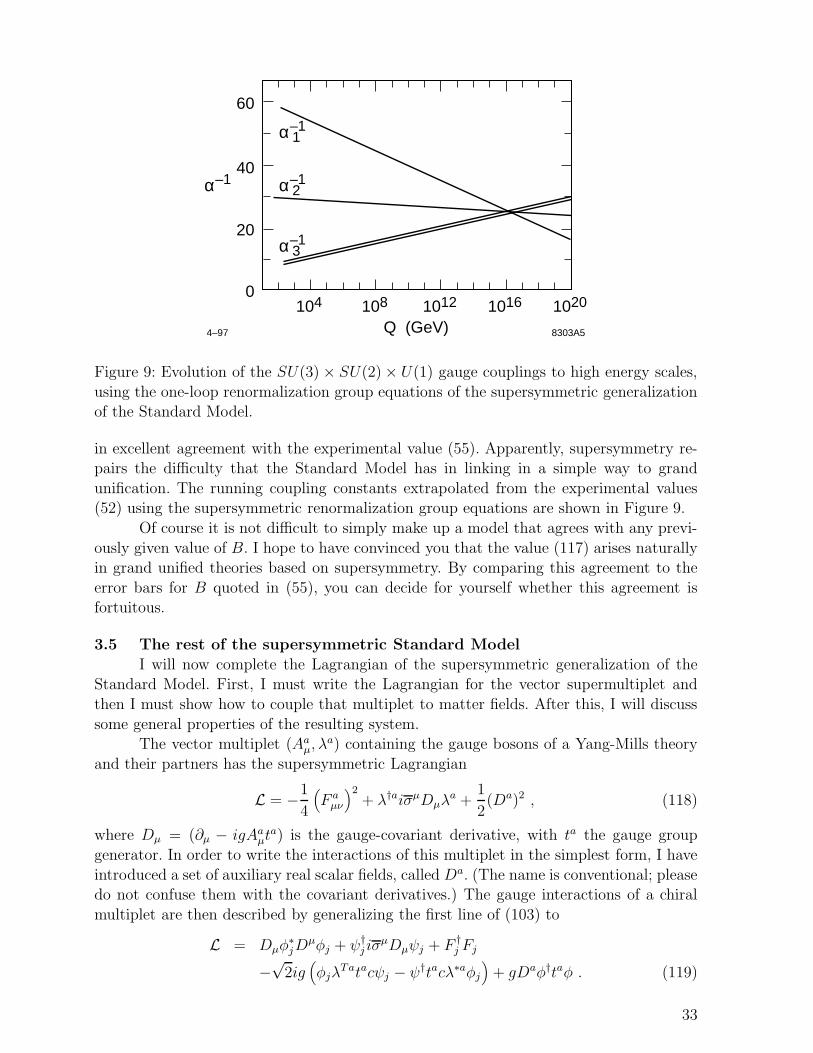
0
20
40
60
104
Q (GeV)4–97 8303A5
108 1012 1016 1020
α–11
α–1α–12
α–13
Figure 9: Evolution of the SU(3) × SU(2) × U(1) gauge couplings to high energy scales,
using the one-loop renormalization group equations of the supersymmetric generalizationof the Standard Model.
in excellent agreement with the experimental value (55). Apparently, supersymmetry re-pairs the difficulty that the Standard Model has in linking in a simple way to grand
unification. The running coupling constants extrapolated from the experimental values(52) using the supersymmetric renormalization group equations are shown in Figure 9.
Of course it is not difficult to simply make up a model that agrees with any previ-
ously given value of B. I hope to have convinced you that the value (117) arises naturallyin grand unified theories based on supersymmetry. By comparing this agreement to the
error bars for B quoted in (55), you can decide for yourself whether this agreement isfortuitous.
3.5 The rest of the supersymmetric Standard Model
I will now complete the Lagrangian of the supersymmetric generalization of theStandard Model. First, I must write the Lagrangian for the vector supermultiplet and
then I must show how to couple that multiplet to matter fields. After this, I will discuss
some general properties of the resulting system.The vector multiplet (Aaµ, λ
a) containing the gauge bosons of a Yang-Mills theory
and their partners has the supersymmetric Lagrangian
L = −1
4
(F aµν
)2+ λ†aiσµDµλ
a +1
2(Da)2 , (118)
where Dµ = (∂µ − igAaµta) is the gauge-covariant derivative, with ta the gauge group
generator. In order to write the interactions of this multiplet in the simplest form, I have
introduced a set of auxiliary real scalar fields, called Da. (The name is conventional; pleasedo not confuse them with the covariant derivatives.) The gauge interactions of a chiral
multiplet are then described by generalizing the first line of (103) to
L = Dµφ∗jD
µφj + ψ†j iσ
µDµψj + F †j Fj
−√
2ig(φjλ
Tatacψj − ψ†tacλ∗aφj)
+ gDaφ†taφ . (119)
33
Eliminating the auxiliary fields using their field equation
Da = −g∑
j
φ†taφ (120)
gives a second contribution to the scalar potential, which should be added to the F-term
(112). This is the D-term
V =g2
2
∑
j
φ†taφ
2
. (121)
As with the F-term, the ground state of this potential is obtained by setting all of the Da
equal to zero, if it is possible. In that case, one obtains a supersymmetric vacuum statewith 〈H〉 = 0.
The full supersymmetric generalization of the Standard Model can be written inthe form
L = Lgauge + Lkin + LYukawa + Lµ . (122)
The first term is the kinetic energy term for the gauge multiplets of SU(3)×SU(2)×U(1).
The second term is the kinetic energy term for quark, lepton, and Higgs chiral multiplets,including gauge couplings of the form (119). The third term is the Yukawa and scalar
interactions given by the second line of (103) using the superpotential (113). The lastterm is that following from an additional gauge-invariant term that we could add to the
superpotential,
∆W = µh1 · h2 . (123)
This term contributes a supersymmetric mass term to the Higgs fields and to their fermions
partners. This term is needed on phenomenological grounds, as I will discuss in Section4.4. The parameter µ is the only new parameter that we have added so far to the Standard
Model.
This Lagrangian does not yet describe a realistic theory. It has exact supersymme-try. Thus, it predicts charged scalars degenerate with the electron and massless fermionic
partners for the photon and gluons. On the other hand, it has some very attrative proper-ties. For the reasons explained below (110), there is no quadratically divergent renormal-
ization of the Higgs boson masses, or of any other mass in the theory. Thus, the radiativecorrection (26), which was such a problem for the Standard Model, is absent in this gen-
eralization. In fact, the only renormalizations in the theory are renormalizations of theSU(3) × SU(2) × U(1) gauge couplings and rescalings of the various quark, lepton, and
Higgs fields. In the next section, I will show that we can modify (122) to maintain thisproperty while making the mass spectrum of the theory more realistic.
The Lagrangian (122) conserves the discrete quantum number
R = (−1)L+Q+2J , (124)
where L is the lepton number, Q = 3B is the quark number, and J is the spin. This quan-
tity is called R-parity, and it is constructed precisely so that R = +1 for the conventionalgauge boson, quark, lepton, and Higgs states while R = −1 for their supersymmetry part-
ners. If R is exactly conserved, supersymmetric particles can only be produced in pairs,
34
and the lightest supersymmetric partner must be absolutely stable. On the other hand, R-
parity can be violated only by adding terms to L which violate baryon- or lepton-number
conservation.It is in fact straightforward to write a consistent R-parity-violating supersymmetric
theory. The following terms which can be added to the superpotential are invariant underSU(3) × SU(2) × U(1) but violate baryon or lepton number:
∆W = λijkB uidjdk
+ λijkL Qi · Ljdk + λijke Li · Ljek + µiLLi · h2 . (125)
A different phenomenology is produced if one adds the baryon-number violating couplings
λB, or if one adds the other couplings written in (125), which violate lepton number. Ifone were to add both types of couplings at once, that would be a disaster, leading to rapid
proton decay.For a full exploration of the phenomenology of supersymmetric theories, we should
investigate both models in which R-parity is conserved, in which the lightest superpartneris stable, and models in which R-parity is violated, in which the lightest superpartner
decays through B- or L- violating interactions. In these lectures, since my plan is topresent illustrative examples rather than a systematic survey, I will restrict my attention
to models with conserved R-parity.
3.6 How to describe supersymmetry breaking
Now we must address the question of how to modify the Lagrangian (122) to obtain
a model that could be realistic. Our problem is that the supersymmetry on which themodel is based is not manifest in the spectrum of particles we see in Nature. So now we
must add new particles or interactions which cause supersymmetry to be spontaneouslybroken.
It would be very attractive if there were a simple model of supersymmetry breaking
that we could connect to the supersymmetric Standard Model. Unfortunately, models ofsupersymmetry breaking are generally not simple. So most studies of supersymmetry
do not invoke the supersymmetry breaking mechanism directly but instead try to treatits consequences phenomenologically. This can be done by adding to (122) terms which
violate supersymmetry but become unimportant at high energy. Some time ago, Grisaruand Girardello [18] listed the terms that one can add to a supersymmetric Lagrangian
without disturbing the cancellation of quadratic divergences in the scalar mass terms.These terms are
Lsoft = −M2j |φj |2 −maλ
Tacλa +Bµh1 · h2 + AW (φ) , (126)
where W is the superpotential (113), plus other possible analytic terms cubic in the scalar
fields φj. These terms give mass to the squarks and sleptons and to the gauginos, movingthe unobserved superpartners to higher energy. Note that terms of the structure φ∗φφ and
the mass term ψT cψ do not appear in (126) because they can regenerate the divergencesof the nonsupersymmetric theory. All of the coefficients in (126) have the dimensions
of (mass) or (mass)2. These new terms in (126) are called soft supersymmetry-breaking
terms. We can build a phenomenological model of supersymmetry by adding to (122) the
various terms in Lsoft with coefficients to be determined by experiment.
35
It is not difficult to understand that it is the new, rather than the familiar, half of
the spectrum of the supersymmetric model that obtains mass from (126). In Section 2.5, I
argued that the particles we see in high-energy experiments are visible only because theyare protected from acquiring very large masses by some symmetry principle . In that dis-
cussion, I invoked only the Standard Model gauge symmetries. In supersymmetric models,we have a more complex situation. In each supermultiplet, one particle is protected from
acquiring mass, as before, by SU(2) × U(1). However, their superpartners—the squarks,sleptons, and gauginos—are protected from obtaining mass only by the supersymmetry
relation to their partner. Thus, if supersymmetry is spontaneously broken, all that is nec-essary to generate masses for these partners is a coupling of the supersymmetry-breaking
expectation values to the Standard Model supermultiplets.This idea suggests a general structure for a realistic supersymmetric model. All
of the phenomena of the model are driven by supersymmetry breaking. First, supersym-metry is broken spontaneously in some new sector of particles at high energy. Then, the
coupling between these particles and the quarks, leptons, and gauge bosons leads to softsupersymmetry-breaking terms for those supermultiplets. It is very tempting to speculate
further that those terms might then give rise to the spontaneous breaking of SU(2)×U(1)
and so to the masses for the W and Z and for the quarks and leptons. I will explain inthe next section how this might happen.
The size of the mass terms in (126) depends on two factors. The first of these is themass scale at which supersymmetry is broken. Saying for definiteness that supersymmetry
breaking is due to the nonzero value of an F auxiliary field, we can denote this scale bywriting 〈F 〉, which has the dimensions of (mass)2. The second factor is the mass of the
bosons or fermions which couple the high-energy sector to the particles of the StandardModel and thus communicate the supersymmetry breaking. I will call this mass M, the
messenger scale. Then the mass parameters that appear in (126) should be of the orderof
mS =〈F 〉M . (127)
If supersymmetry indeed gives the mechanism of electroweak symmetry breaking, thenmS should be of the order of 1 TeV. A case that is often discussed in the literature is that
in which the messenger is supergravity. In that case, M is the Planck mass m Pl, equal to1019 GeV, and 〈F 〉 ∼ 1011 (GeV)2. Alternatively, both 〈F 〉 and M could be of the order
of a few TeV.The detailed form of the soft supersymmetry-breaking terms depends on the under-
lying model that has generated them. If one allows these terms to have their most generalform (including arbitrary flavor- and CP-violating interactions, they contain about 120
new parameters. However, any particular model of supersymmetry breaking generates
a specific set of these soft terms with some observable regularities. One of our goals inSection 4 of these lectures will be to understand how to determine the soft parameters
experimentally and thus uncover the patterns which govern their construction.
3.7 Electroweak symmetry breaking from supersymmetry
There is a subtlety in trying to determine the pattern of the soft parameters exper-imentally. Like all other coupling constants in a supersymmetric theory, these parameters
run under the influence of the renormalization group equations. Thus, the true underlying
36
pattern might not be seen directly at the TeV energy scale. Rather, it might be necessary
to extrapolate the measured values of parameters to higher energy to look for regularities.
The situation here is very similar to that of the Standard Model coupling con-stants. The underlying picture which leads to the values of the SU(3) × SU(2) × U(1)
coupling constants is not very obvious from the data (52). Only when these data areextrapolated to very high energy using the renormalization group do we see evidence for
their unification. Obviously, such evidence must be indirect. On the other hand, the dis-covery of supersymmetric particles, and the discovery that these particles showed other
unification relations—with the same unification mass scale—would give powerful supportto this picture.
I will discuss general systematics of the renormalization-group running of the softparameters in Section 4.2. But there is one set of renormalization group equations that
I would like to call your attention to right away. These are the equations for the softmass of the Higgs boson and the squarks which are most strongly coupled to it. We saw
in Section 2.6 that the top quark Yukawa coupling was sufficiently large that it couldhave an important effect in renormalization group evolution. Let us consider, then, the
evolution equations for the three scalars that interact through this coupling, the Higgs
boson h2, the scalar top Qt = tL, and the scalar top tR. The most important terms inthese equations are the following:
d
d logQM2
h =1
(4π)2
{3λ2
t (M2h +M2
Q +M2t ) + · · ·
}
d
d logQM2
Q =1
(4π)2
{2λ2
t (M2h +M2
Q +M2t ) −
32
3g23m
23 · · ·
}
d
d logQM2
t =1
(4π)2
{3λ2
t (M2h +M2
Q +M2t ) −
32
3g23m
23 + · · ·
},
(128)
where g3 is the QCD coupling, m3 is the mass of the gluino, and the omitted terms are
of electroweak strength. The last two equations exhibit the competition between the topquark Yukawa coupling and QCD renormalizations which we saw earlier in (61) and (64).
The supersymmetric QCD couplings cause the masses of the Qt and tR to increase at lowenergies, while the effect of λt causes all three masses to decrease.
Indeed, if the Qt and tR masses stay large, the equations (128) predict that M2h
should go down through zero and become negative [19]. Thus, if all scalar mass parameters
are initially positive at high energy scales, these equations imply that the Higgs bosonh2 will acquire a negative parameter and thus an instability to electroweak symmetry
breaking. An example of the solution to the full set of renormalization group equations,exhibiting the instability in M2
h , is shown in Figure 10 [20].
At first sight, it might have been any of the scalar fields in the theory whose
potential would be unstable by renormalization group evolution. But the Higgs scalar h2
has the strongest instability if the top quark is heavy. In this way, the supersymmetric
extension of the Standard Model naturally contains the essential feature that we set outto find, a physical mechanism for electroweak symmetry breaking. As a bonus, we find
that this mechanism is closely associated with the heaviness of the top quark.If you have been patient through all of the formalism I have presented in this section,
you now see that your patience has paid off. It was not obvious when we started that
37
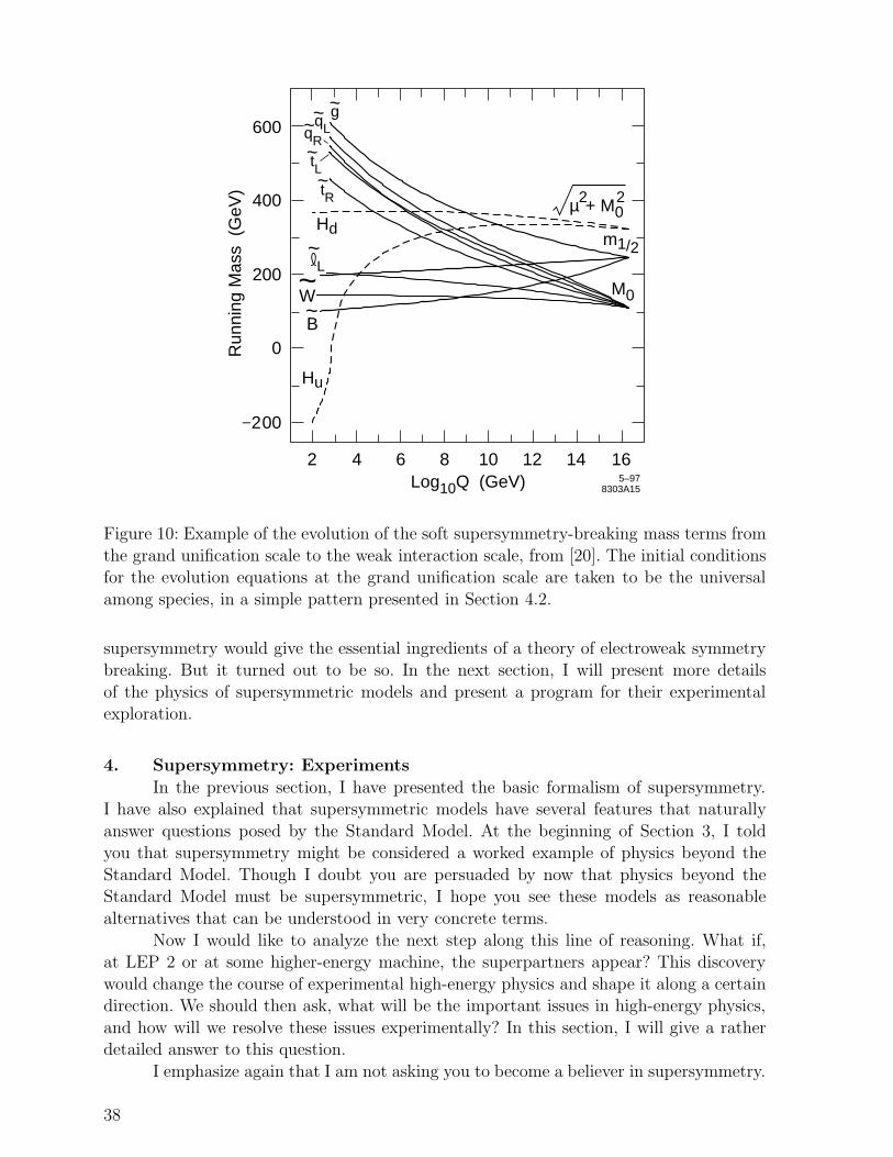
2
Hu
Hd
B~
L~
W~
g~qL~
tL~
tR~
qR~
4 6 8
Run
ning
Mas
s (
GeV
)
M0
m1/2
10Log10Q (GeV)
12 14 165–97
8303A15
600
400
200
0
–200
µ + M0
22
Figure 10: Example of the evolution of the soft supersymmetry-breaking mass terms from
the grand unification scale to the weak interaction scale, from [20]. The initial conditionsfor the evolution equations at the grand unification scale are taken to be the universal
among species, in a simple pattern presented in Section 4.2.
supersymmetry would give the essential ingredients of a theory of electroweak symmetrybreaking. But it turned out to be so. In the next section, I will present more details
of the physics of supersymmetric models and present a program for their experimentalexploration.
4. Supersymmetry: Experiments
In the previous section, I have presented the basic formalism of supersymmetry.I have also explained that supersymmetric models have several features that naturally
answer questions posed by the Standard Model. At the beginning of Section 3, I toldyou that supersymmetry might be considered a worked example of physics beyond the
Standard Model. Though I doubt you are persuaded by now that physics beyond theStandard Model must be supersymmetric, I hope you see these models as reasonable
alternatives that can be understood in very concrete terms.
Now I would like to analyze the next step along this line of reasoning. What if,at LEP 2 or at some higher-energy machine, the superpartners appear? This discovery
would change the course of experimental high-energy physics and shape it along a certaindirection. We should then ask, what will be the important issues in high-energy physics,
and how will we resolve these issues experimentally? In this section, I will give a ratherdetailed answer to this question.
I emphasize again that I am not asking you to become a believer in supersymmetry.
38
A different discovery about physics beyond the Standard Model would change the focus
of high-energy physics in a different direction. But we will learn more by choosing a
particular direction and studying its far-reaching implications than by trying to reachvague but general conclusions. I will strike off in a different direction in Section 5.
On the other hand, I hope you are not put off by the complexity of the supersym-metric Standard Model. It is true that this model has many ingredients and a very large
content of new undiscovered particles. On the other hand, the model develops naturallyfrom a single physical idea. I argued in Section 2.2 that this structure, a complex phe-
nomenology built up around a definite principle of physics, is seen often in Nature. Itleads to a more attractive solution to the problems of the Standard Model than a model
whose only virtue is minimality.It is true that, in models with complex consequences, it may not be easy to see the
underlying structure in the experimental data. This is the challenge that experimenterswill face. I will now discuss how we can meet this challenge for the particular case in
which the physics beyond the Standard Model is supersymmetric.
4.1 More about soft supersymmetry breaking
As we discussed in Section 3.6, a realistic supersymmetric theory has a Lagrangian
of the formL = Lgauge + Lkin + LYukawa + Lµ + Lsoft . (129)
Of the various terms listed here, the first three contain only couplings that are already
present in the Lagrangian of the Standard Model. The fourth term contains one newparameter µ. The last term, however, contains a very large number of new parameters.
I have already explained that one should not be afraid of seeing a large number of
undetermined parameters here. The same proliferation of parameters occurs in any theorywith a certain level of complexity when viewed from below. The low-energy scattering
amplitudes of QCD, for example, contain many parameters which turn out to be themasses and decay constants of hadronic resonances. If it is possible to measure these
parameters, we will obtain a large amount of new information.In thinking about the values of the soft supersymmetry-breaking parameters, there
are two features that we should take into account. The first is that the soft parametersobey renormalization group equations. Thus, they potentially change significantly from
their underlying values at the messenger scale defined in (127) to their physical valuesobservable at the TeV scale. We have seen in Section 3.7 that these changes can have
important physical consequences. In the next section, I will describe the renormalizationgroup evolution of the supersymmetry-breaking mass terms in more detail, and we will
use our understanding of this evolution to work out some general predictions for thesuperparticle spectrum.
The second feature is that there are strong constraints on the flavor structure of soft
supersymmetry breaking terms which come from constraints on flavor-changing neutralcurrent processes. In (126), I have written independent mass terms for each of the scalar
fields. In principle, I could also have written mass terms that mixed these fields. However,if we write the scalars in the basis in which the quark masses are diagonalized, we must
not find substantial off-diagonal terms. A mixing
∆L = ∆M2ds
†d , (130)
39
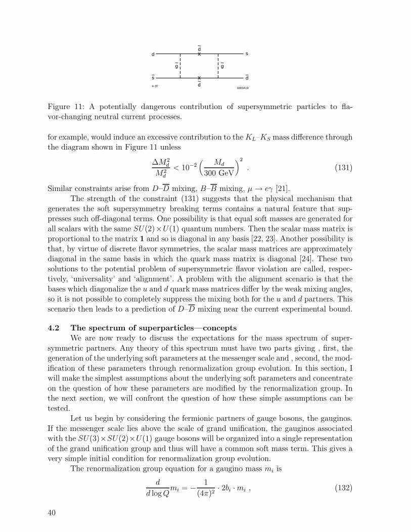
4–978303A19
dd~
g~
g~
d~
d
s
s x
x
Figure 11: A potentially dangerous contribution of supersymmetric particles to fla-vor-changing neutral current processes.
for example, would induce an excessive contribution to theKL–KS mass difference throughthe diagram shown in Figure 11 unless
∆M2d
M2d
< 10−2(
Md
300 GeV
)2
. (131)
Similar constraints arise from D–D mixing, B–B mixing, µ → eγ [21].The strength of the constraint (131) suggests that the physical mechanism that
generates the soft supersymmetry breaking terms contains a natural feature that sup-presses such off-diagonal terms. One possibility is that equal soft masses are generated for
all scalars with the same SU(2)×U(1) quantum numbers. Then the scalar mass matrix isproportional to the matrix 1 and so is diagonal in any basis [22, 23]. Another possibility is
that, by virtue of discrete flavor symmetries, the scalar mass matrices are approximatelydiagonal in the same basis in which the quark mass matrix is diagonal [24]. These two
solutions to the potential problem of supersymmetric flavor violation are called, respec-tively, ‘universality’ and ‘alignment’. A problem with the alignment scenario is that the
bases which diagonalize the u and d quark mass matrices differ by the weak mixing angles,so it is not possible to completely suppress the mixing both for the u and d partners. This
scenario then leads to a prediction of D–D mixing near the current experimental bound.
4.2 The spectrum of superparticles—concepts
We are now ready to discuss the expectations for the mass spectrum of super-
symmetric partners. Any theory of this spectrum must have two parts giving , first, thegeneration of the underlying soft parameters at the messenger scale and , second, the mod-
ification of these parameters through renormalization group evolution. In this section, Iwill make the simplest assumptions about the underlying soft parameters and concentrate
on the question of how these parameters are modified by the renormalization group. Inthe next section, we will confront the question of how these simple assumptions can be
tested.Let us begin by considering the fermionic partners of gauge bosons, the gauginos.
If the messenger scale lies above the scale of grand unification, the gauginos associatedwith the SU(3)×SU(2)×U(1) gauge bosons will be organized into a single representation
of the grand unification group and thus will have a common soft mass term. This gives avery simple initial condition for renormalization group evolution.
The renormalization group equation for a gaugino mass mi is
d
d logQmi = − 1
(4π)2· 2bi ·mi , (132)
40
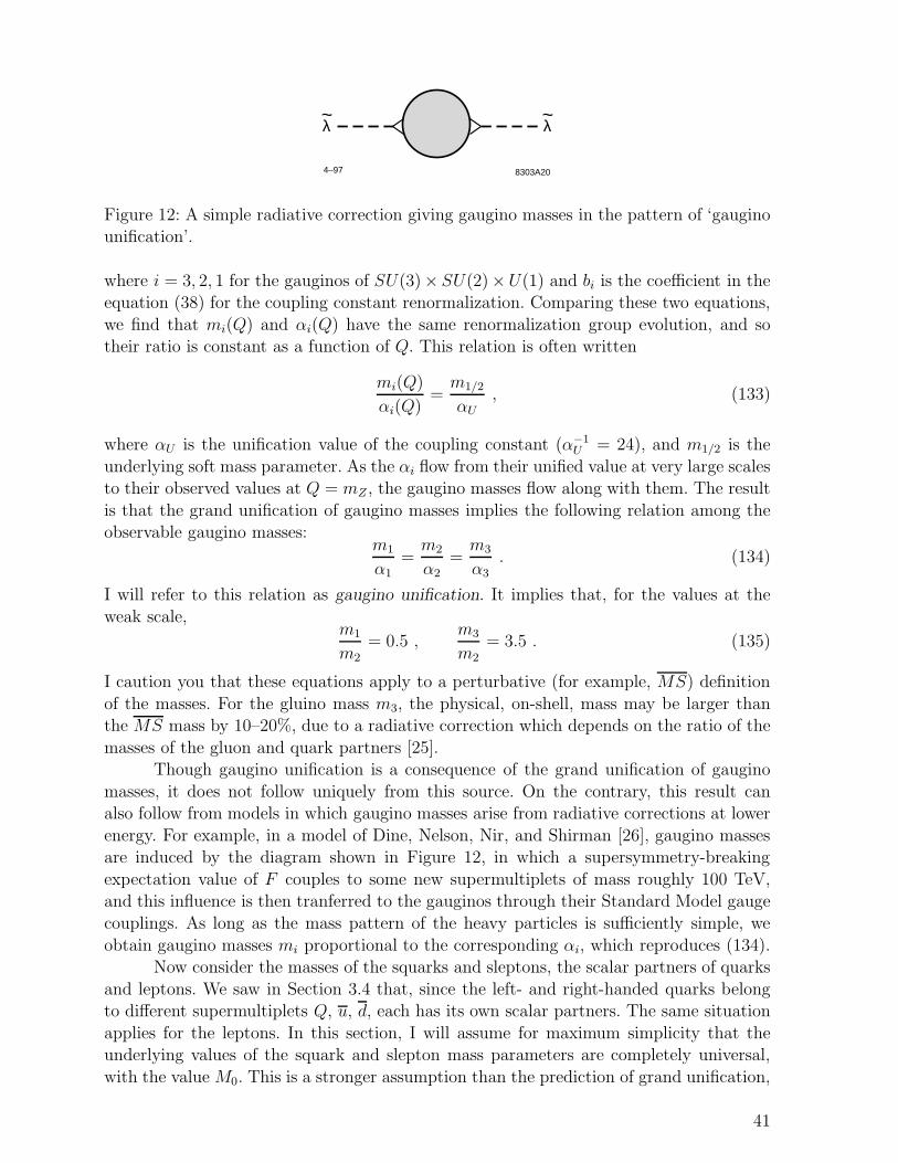
4–97 8303A20
~λ~λ
Figure 12: A simple radiative correction giving gaugino masses in the pattern of ‘gauginounification’.
where i = 3, 2, 1 for the gauginos of SU(3)× SU(2)×U(1) and bi is the coefficient in theequation (38) for the coupling constant renormalization. Comparing these two equations,
we find that mi(Q) and αi(Q) have the same renormalization group evolution, and sotheir ratio is constant as a function of Q. This relation is often written
mi(Q)
αi(Q)=m1/2
αU, (133)
where αU is the unification value of the coupling constant (α−1U = 24), and m1/2 is the
underlying soft mass parameter. As the αi flow from their unified value at very large scalesto their observed values at Q = mZ , the gaugino masses flow along with them. The result
is that the grand unification of gaugino masses implies the following relation among theobservable gaugino masses:
m1
α1=m2
α2=m3
α3. (134)
I will refer to this relation as gaugino unification. It implies that, for the values at the
weak scale,m1
m2
= 0.5 ,m3
m2
= 3.5 . (135)
I caution you that these equations apply to a perturbative (for example, MS) definition
of the masses. For the gluino mass m3, the physical, on-shell, mass may be larger thanthe MS mass by 10–20%, due to a radiative correction which depends on the ratio of the
masses of the gluon and quark partners [25].Though gaugino unification is a consequence of the grand unification of gaugino
masses, it does not follow uniquely from this source. On the contrary, this result canalso follow from models in which gaugino masses arise from radiative corrections at lower
energy. For example, in a model of Dine, Nelson, Nir, and Shirman [26], gaugino massesare induced by the diagram shown in Figure 12, in which a supersymmetry-breaking
expectation value of F couples to some new supermultiplets of mass roughly 100 TeV,and this influence is then tranferred to the gauginos through their Standard Model gauge
couplings. As long as the mass pattern of the heavy particles is sufficiently simple, we
obtain gaugino masses mi proportional to the corresponding αi, which reproduces (134).Now consider the masses of the squarks and sleptons, the scalar partners of quarks
and leptons. We saw in Section 3.4 that, since the left- and right-handed quarks belongto different supermultiplets Q, u, d, each has its own scalar partners. The same situation
applies for the leptons. In this section, I will assume for maximum simplicity that theunderlying values of the squark and slepton mass parameters are completely universal,
with the value M0. This is a stronger assumption than the prediction of grand unification,
41
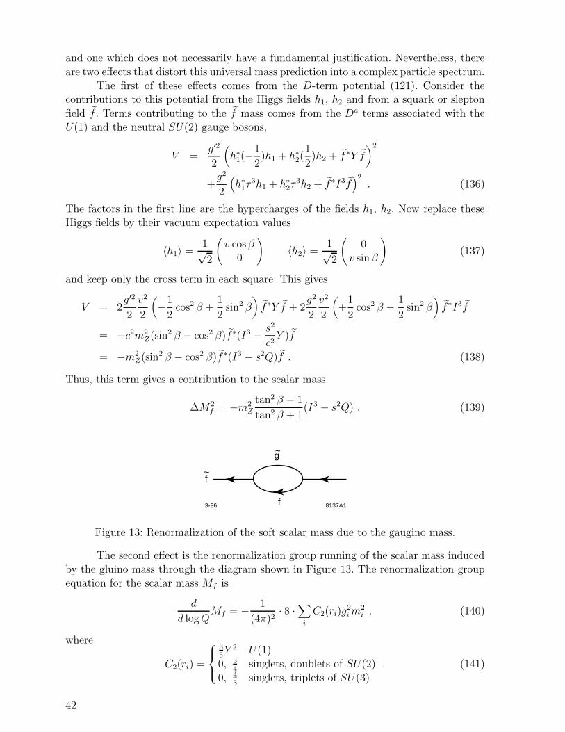
and one which does not necessarily have a fundamental justification. Nevertheless, there
are two effects that distort this universal mass prediction into a complex particle spectrum.
The first of these effects comes from the D-term potential (121). Consider thecontributions to this potential from the Higgs fields h1, h2 and from a squark or slepton
field f . Terms contributing to the f mass comes from the Da terms associated with theU(1) and the neutral SU(2) gauge bosons,
V =g′2
2
(h∗1(−
1
2)h1 + h∗2(
1
2)h2 + f ∗Y f
)2
+g2
2
(h∗1τ
3h1 + h∗2τ3h2 + f ∗I3f
)2. (136)
The factors in the first line are the hypercharges of the fields h1, h2. Now replace theseHiggs fields by their vacuum expectation values
〈h1〉 =1√2
(v cosβ
0
)〈h2〉 =
1√2
(0
v sin β
)(137)
and keep only the cross term in each square. This gives
V = 2g′2
2
v2
2
(−1
2cos2 β +
1
2sin2 β
)f ∗Y f + 2
g2
2
v2
2
(+
1
2cos2 β − 1
2sin2 β
)f ∗I3f
= −c2m2Z(sin2 β − cos2 β)f ∗(I3 − s2
c2Y )f
= −m2Z(sin2 β − cos2 β)f ∗(I3 − s2Q)f . (138)
Thus, this term gives a contribution to the scalar mass
∆M2f = −m2
Z
tan2 β − 1
tan2 β + 1(I3 − s2Q) . (139)
f~
~
f
g
3-96 8137A1
Figure 13: Renormalization of the soft scalar mass due to the gaugino mass.
The second effect is the renormalization group running of the scalar mass induced
by the gluino mass through the diagram shown in Figure 13. The renormalization groupequation for the scalar mass Mf is
d
d logQMf = − 1
(4π)2· 8 ·
∑
i
C2(ri)g2im
2i , (140)
where
C2(ri) =
35Y 2 U(1)
0, 34
singlets, doublets of SU(2)
0, 43
singlets, triplets of SU(3). (141)
42
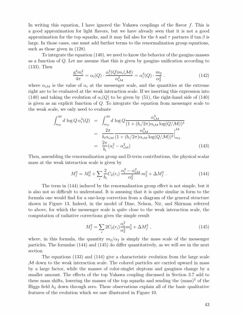
In writing this equation, I have ignored the Yukawa couplings of the flavor f . This is
a good approximation for light flavors, but we have already seen that it is not a good
approximation for the top squarks, and it may fail also for the b and τ partners if tan β islarge. In those cases, one must add further terms to the renormalization group equations,
such as those given in (128).To integrate the equation (140), we need to know the behavior of the gaugino masses
as a function of Q. Let me assume that this is given by gaugino unification according to(133). Then
g2im
2i
4π= αi(Q) · α
2i (Q)mi(M)
α2iM
= α3i (Q) · m2
α22
. (142)
where αiM is the value of αi at the messenger scale, and the quantities at the extreme
right are to be evaluated at the weak interaction scale. If we inserting this expression into(140) and taking the evolution of αi(Q) to be given by (51), the right-hand side of (140)
is given as an explicit function of Q. To integrate the equation from messenger scale to
the weak scale, we only need to evaluate∫ M
mZ
d logQα3i (Q) =
∫ M
mZ
d logQα3iM
(1 + (bi/2π)αiM log(Q/M))3
=2π
biαiM
α3iM
(1 + (bi/2π)αiM log(Q/M))2
∣∣∣∣M
mZ
=2π
bi(α2
i − α2iM) (143)
Then, assembling the renormalization group and D-term contributions, the physical scalar
mass at the weak interaction scale is given by
M2f = M2
0 +∑
i
2
biC2(ri)
α2i − α2
iMα2
2
m22 + ∆M2
f . (144)
The term in (144) induced by the renormalization group effect is not simple, but itis also not so difficult to understand. It is amusing that it is quite similar in form to the
formula one would find for a one-loop correction from a diagram of the general structureshown in Figure 13. Indeed, in the model of Dine, Nelson, Nir, and Shirman referred
to above, for which the messenger scale is quite close to the weak interaction scale, thecomputation of radiative corrections gives the simple result
M2f =
∑
i
2C2(ri)α2i
α22
m22 + ∆M2
f , (145)
where, in this formula, the quantity m2/α2 is simply the mass scale of the messengerparticles. The formulae (144) and (145) do differ quantitatively, as we will see in the next
section.
The equations (133) and (144) give a characteristic evolution from the large scaleM down to the weak interaction scale. The colored particles are carried upward in mass
by a large factor, while the masses of color-singlet sleptons and gauginos change by asmaller amount. The effects of the top Yukawa coupling discussed in Section 3.7 add to
these mass shifts, lowering the masses of the top squarks and sending the (mass)2 of theHiggs field h2 down through zero. These observations explain all of the basic qualitative
features of the evolution which we saw illustrated in Figure 10.
43
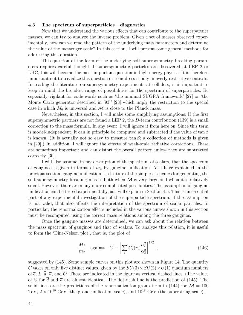
4.3 The spectrum of superparticles—diagnostics
Now that we understand the various effects that can contribute to the superpartner
masses, we can try to analyze the inverse problem: Given a set of masses observed exper-imentally, how can we read the pattern of the underlying mass parameters and determine
the value of the messenger scale? In this section, I will present some general methods foraddressing this question.
This question of the form of the underlying soft-supersymmetry breaking param-eters requires careful thought. If supersymmetric particles are discovered at LEP 2 or
LHC, this will become the most important question in high-energy physics. It is thereforeimportant not to trivialize this question or to address it only in overly restrictive contexts.
In reading the literature on supersymmetry experiments at colliders, it is important tokeep in mind the broadest range of possibilities for the spectrum of superparticles. Be
especially vigilant for code-words such as ‘the minimal SUGRA framework’ [27] or ‘theMonte Carlo generator described in [93]’ [28] which imply the restriction to the special
case in which M0 is universal and M is close to the Planck mass.
Nevertheless, in this section, I will make some simplifying assumptions. If the firstsupersymmetric partners are not found a LEP 2, the D-term contribution (139) is a small
correction to the mass formula. In any event, I will ignore it from here on. Since this termis model-independent, it can in principle be computed and subtracted if the value of tanβ
is known. (It is actually not so easy to measure tanβ; a collection of methods is givenin [29].) In addition, I will ignore the effects of weak-scale radiative corrections. These
are sometimes important and can distort the overall pattern unless they are subtractedcorrectly [30].
I will also assume, in my description of the spectrum of scalars, that the spectrumof gauginos is given in terms of m2 by gaugino unification. As I have explained in the
previous section, gaugino unification is a feature of the simplest schemes for generating thesoft supersymmetry-breaking masses both when M is very large and when it is relatively
small. However, there are many more complicated possibilities. The assumption of gauginounification can be tested experimentally, as I will explain in Section 4.5. This is an essential
part of any experimental investigation of the superparticle spectrum. If the assumption
is not valid, that also affects the interpretation of the spectrum of scalar particles. Inparticular, the renormalization effects included in the various curves shown in this section
must be recomputed using the correct mass relations among the three gauginos.Once the gaugino masses are determined, we can ask about the relation between
the mass spectrum of gauginos and that of scalars. To analyze this relation, it is usefulto form the ‘Dine-Nelson plot’, that is, the plot of
Mf
m2against C ≡
[∑
i
C2(ri)α2i
α22
]1/2
, (146)
suggested by (145). Some sample curves on this plot are shown in Figure 14. The quantity
C takes on only five distinct values, given by the SU(3)×SU(2)×U(1) quantum numbersof e, L, d, u, and Q. These are indicated in the figure as vertical dashed lines. (The values
of C for d and u are almost identical. The dot-dash line is the prediction of (145). Thesolid lines are the predictions of the renormalization group term in (144) for M = 100
TeV, 2 × 10¹⁶ GeV (the grand unification scale), and 1018 GeV (the superstring scale).
44
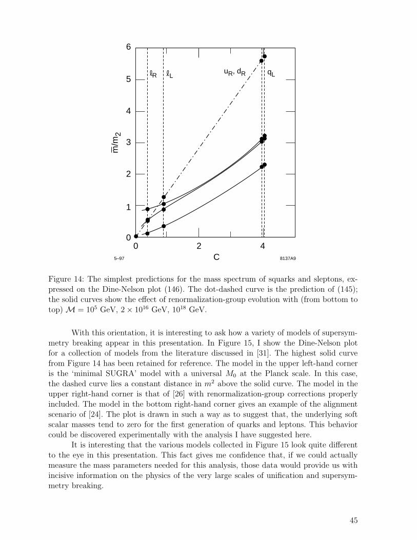
6
5
4
3
m/m
2
2
1
00 2
C4
5–97 8137A9
uR, dR qL R L
Figure 14: The simplest predictions for the mass spectrum of squarks and sleptons, ex-
pressed on the Dine-Nelson plot (146). The dot-dashed curve is the prediction of (145);the solid curves show the effect of renormalization-group evolution with (from bottom to
top) M = 105 GeV, 2 × 10¹⁶ GeV, 1018 GeV.
With this orientation, it is interesting to ask how a variety of models of supersym-
metry breaking appear in this presentation. In Figure 15, I show the Dine-Nelson plotfor a collection of models from the literature discussed in [31]. The highest solid curve
from Figure 14 has been retained for reference. The model in the upper left-hand corneris the ‘minimal SUGRA’ model with a universal M0 at the Planck scale. In this case,
the dashed curve lies a constant distance in m2 above the solid curve. The model in theupper right-hand corner is that of [26] with renormalization-group corrections properly
included. The model in the bottom right-hand corner gives an example of the alignment
scenario of [24]. The plot is drawn in such a way as to suggest that, the underlying softscalar masses tend to zero for the first generation of quarks and leptons. This behavior
could be discovered experimentally with the analysis I have suggested here.It is interesting that the various models collected in Figure 15 look quite different
to the eye in this presentation. This fact gives me confidence that, if we could actuallymeasure the mass parameters needed for this analysis, those data would provide us with
incisive information on the physics of the very large scales of unification and supersym-metry breaking.
45
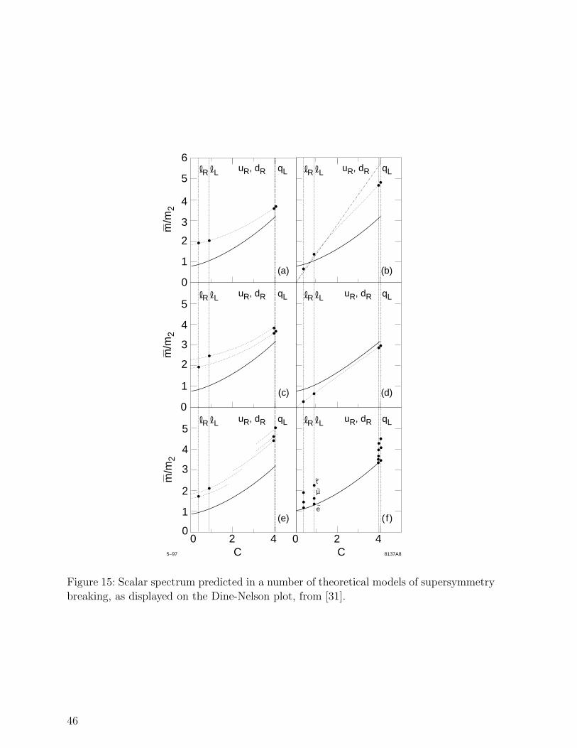
0 2C
48137A8
τµ
e~
~
~
6
5
4
3
m/m
2
2
1
0
uR, dR uR, dR qL qL R L R L
uR, dR uR, dR qL qL R L R L
uR, dR uR, dR qL qL R L R L
5
4
3
m/m
2
2
1
0
5
4
3
m/m
2
2
1
00 2
C4
5–97
(e) ( f )
(c) (d)
(a) (b)
Figure 15: Scalar spectrum predicted in a number of theoretical models of supersymmetry
breaking, as displayed on the Dine-Nelson plot, from [31].
46
4.4 The superpartners of W and Higgs
Now that we have framed the problem of measuring the mass spectrum of super-particles, we must address the question of how this can be done. What are the signatures
of the presence of supersymmetric particles, and how can we translate from the charac-
teristics of observable processes to the values of the parameters of which determine thesupersymmetry spectrum?
I will discuss the signatures and decay schemes for superparticles in the next section.First, though, we must discuss a complication which needs to be taken into account in
this phenomenology.After SU(2) × U(1) symmetry-breaking, any two particles with the same color,
charge, and spin can mix. Thus, the spin-12
supersymmetric partners of the W bosons andthe charged Higgs bosons can mix with one another. Similarly, the partners of the γ, Z0,
h01, and h0
2 enter into a 4 × 4 mixing problem.Consider first the mixing problem of the charged fermions. The mass terms for
these fermions arise from the gaugino-Higgs coupling in (119), the soft gaugino mass termin (126), and the fermion mass term arising from the superpotential (123). The relevant
terms from the Lagrangian are
∆L = −√
2ig
2
(h0
2w−T ch+
2 − h−T1 cw+h01
)
−m2w−T cw+ + µh−T1 ch+
2 . (147)
If we replace h01 and h0
2 by their vacuum expectation values in (137), these terms take the
form
∆L = − ( w− ih−1 )T cm
(w+
ih+2
), (148)
where m is the mass matrix
m =
(m2
√2mW sin β√
2mW cosβ µ
)(149)
The physical massive fermions are the eigenstates of this mass matrix. They are calledcharginos, χ±
1,2, where 1 labels the lighter state. More precisely, the charginos χ+1 , χ+
2
are the linear combinations that diagonalize the matrix m†m, and χ−1 , χ−
2 are the linearcombinations that diagonalize the matrix mm†.
The diagonalization of the matrix (149) is especially simple in the limit in whichthe supersymmetry parameters m2 and µ are large compared to mW . In the region µ >
m2 ≫ mW , χ+1 is approximately w+, with mass m1 ≈ m2, while χ+
2 is approximatelyh+
2 , with mass m2 ≈ µ. For m2 > µ ≫ mW , the content of χ+1 and χ+
2 reverses. More
generally, we refer to the region of parameters in which χ+1 is mainly w+ as the gaugino
region, and that in which χ+1 is mainly h+
2 as the Higgsino region. If charginos are foundare LEP 2, it is quite likely that they may be mixtures of gaugino and Higgsino; however,
the region of parameters in which the charginos are substantially mixed decreases as themass increases. The contours of constant χ+
1 mass in the (µ,m2) plane, for tan β = 4 are
shown in Figure 16.An analysis similar to that leading to (149) gives the mass matrix of the neutral
fermionic partners. This is a 4 × 4 matrix acting on the vector (b, w3, ih01, ih
02), where b
47
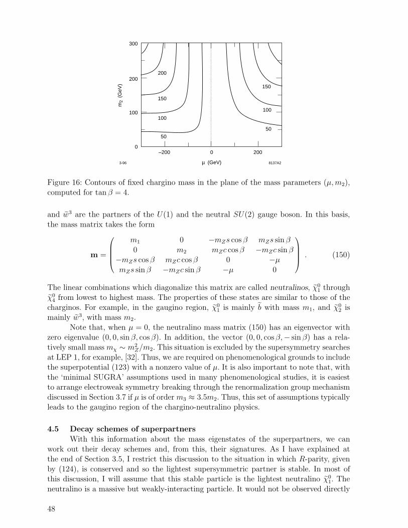
300
200200
150
150
100
100
50
50
100
00
µ (GeV)
m2
(GeV
)
–200 200
3-96 8137A2
Figure 16: Contours of fixed chargino mass in the plane of the mass parameters (µ,m2),
computed for tan β = 4.
and w3 are the partners of the U(1) and the neutral SU(2) gauge boson. In this basis,
the mass matrix takes the form
m =
m1 0 −mZs cosβ mZs sin β
0 m2 mZc cosβ −mZc sin β−mZs cosβ mZc cosβ 0 −µmZs sin β −mZc sin β −µ 0
. (150)
The linear combinations which diagonalize this matrix are called neutralinos, χ01 through
χ04 from lowest to highest mass. The properties of these states are similar to those of the
charginos. For example, in the gaugino region, χ01 is mainly b with mass m1, and χ0
2 ismainly w3, with mass m2.
Note that, when µ = 0, the neutralino mass matrix (150) has an eigenvector withzero eigenvalue (0, 0, sinβ, cosβ). In addition, the vector (0, 0, cosβ,− sin β) has a rela-
tively small mass mχ ∼ m2Z/m2. This situation is excluded by the supersymmetry searches
at LEP 1, for example, [32]. Thus, we are required on phenomenological grounds to includethe superpotential (123) with a nonzero value of µ. It is also important to note that, with
the ‘minimal SUGRA’ assumptions used in many phenomenological studies, it is easiestto arrange electroweak symmetry breaking through the renormalization group mechanism
discussed in Section 3.7 if µ is of order m3 ≈ 3.5m2. Thus, this set of assumptions typicallyleads to the gaugino region of the chargino-neutralino physics.
4.5 Decay schemes of superpartners
With this information about the mass eigenstates of the superpartners, we can
work out their decay schemes and, from this, their signatures. As I have explained atthe end of Section 3.5, I restrict this discussion to the situation in which R-parity, given
by (124), is conserved and so the lightest supersymmetric partner is stable. In most ofthis discussion, I will assume that this stable particle is the lightest neutralino χ0
1. The
neutralino is a massive but weakly-interacting particle. It would not be observed directly
48
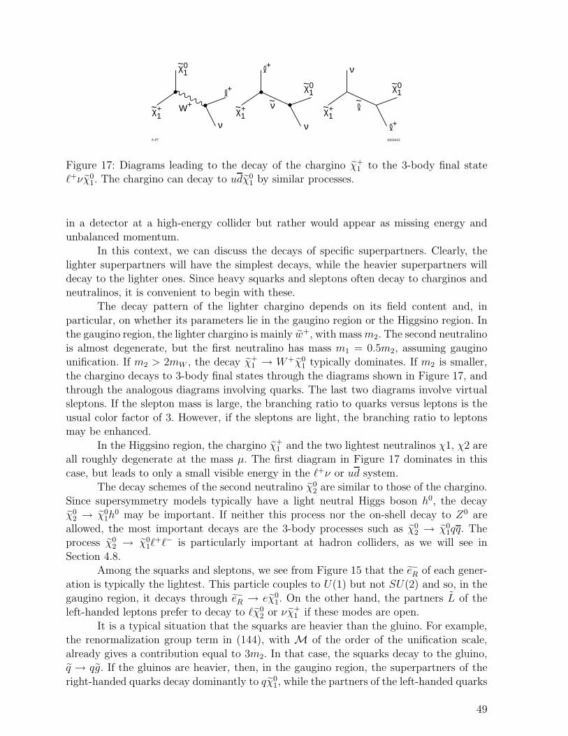
4–97 8303A23
W+
+
0~
~~ν
ν
νν
χ1
0~χ10~χ1
+~χ1+~χ1
+~χ1
+
+
Figure 17: Diagrams leading to the decay of the chargino χ+1 to the 3-body final state
ℓ+νχ01. The chargino can decay to udχ0
1 by similar processes.
in a detector at a high-energy collider but rather would appear as missing energy and
unbalanced momentum.In this context, we can discuss the decays of specific superpartners. Clearly, the
lighter superpartners will have the simplest decays, while the heavier superpartners willdecay to the lighter ones. Since heavy squarks and sleptons often decay to charginos and
neutralinos, it is convenient to begin with these.The decay pattern of the lighter chargino depends on its field content and, in
particular, on whether its parameters lie in the gaugino region or the Higgsino region. Inthe gaugino region, the lighter chargino is mainly w+, with massm2. The second neutralino
is almost degenerate, but the first neutralino has mass m1 = 0.5m2, assuming gauginounification. If m2 > 2mW , the decay χ+
1 → W+χ01 typically dominates. If m2 is smaller,
the chargino decays to 3-body final states through the diagrams shown in Figure 17, and
through the analogous diagrams involving quarks. The last two diagrams involve virtualsleptons. If the slepton mass is large, the branching ratio to quarks versus leptons is the
usual color factor of 3. However, if the sleptons are light, the branching ratio to leptonsmay be enhanced.
In the Higgsino region, the chargino χ+1 and the two lightest neutralinos χ1, χ2 are
all roughly degenerate at the mass µ. The first diagram in Figure 17 dominates in this
case, but leads to only a small visible energy in the ℓ+ν or ud system.The decay schemes of the second neutralino χ0
2 are similar to those of the chargino.
Since supersymmetry models typically have a light neutral Higgs boson h0, the decayχ0
2 → χ01h
0 may be important. If neither this process nor the on-shell decay to Z0 are
allowed, the most important decays are the 3-body processes such as χ02 → χ0
1qq. Theprocess χ0
2 → χ01ℓ
+ℓ− is particularly important at hadron colliders, as we will see in
Section 4.8.Among the squarks and sleptons, we see from Figure 15 that the e−R of each gener-
ation is typically the lightest. This particle couples to U(1) but not SU(2) and so, in the
gaugino region, it decays through e−R → eχ01. On the other hand, the partners L of the
left-handed leptons prefer to decay to ℓχ02 or νχ+
1 if these modes are open.
It is a typical situation that the squarks are heavier than the gluino. For example,the renormalization group term in (144), with M of the order of the unification scale,
already gives a contribution equal to 3m2. In that case, the squarks decay to the gluino,q → qg. If the gluinos are heavier, then, in the gaugino region, the superpartners of the
right-handed quarks decay dominantly to qχ01, while the partners of the left-handed quarks
49
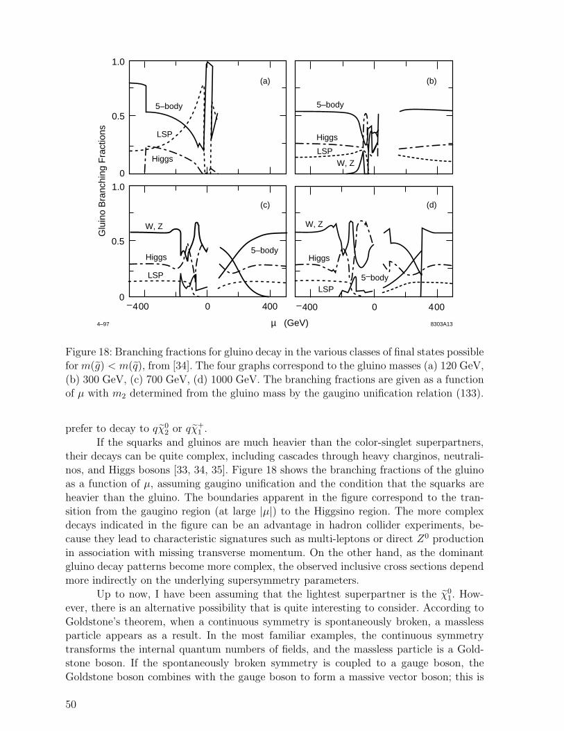
µ (GeV)
Glu
ino
Bra
nchi
ng F
ract
ions
0
4–97
0
8303A13
0.5
–400
Higgs
LSP
5–body
W, Z
(c)
5–body
LSP
Higgs
(a)
0
0.5
1.0
Higgs
LSP
W, Z
(d)
4000–400400
5–body
W, Z
Higgs
(b)
1.0
5–body
LSP
Figure 18: Branching fractions for gluino decay in the various classes of final states possiblefor m(g) < m(q), from [34]. The four graphs correspond to the gluino masses (a) 120 GeV,
(b) 300 GeV, (c) 700 GeV, (d) 1000 GeV. The branching fractions are given as a functionof µ with m2 determined from the gluino mass by the gaugino unification relation (133).
prefer to decay to qχ02 or qχ+
1 .
If the squarks and gluinos are much heavier than the color-singlet superpartners,their decays can be quite complex, including cascades through heavy charginos, neutrali-
nos, and Higgs bosons [33, 34, 35]. Figure 18 shows the branching fractions of the gluinoas a function of µ, assuming gaugino unification and the condition that the squarks are
heavier than the gluino. The boundaries apparent in the figure correspond to the tran-sition from the gaugino region (at large |µ|) to the Higgsino region. The more complex
decays indicated in the figure can be an advantage in hadron collider experiments, be-cause they lead to characteristic signatures such as multi-leptons or direct Z0 production
in association with missing transverse momentum. On the other hand, as the dominantgluino decay patterns become more complex, the observed inclusive cross sections depend
more indirectly on the underlying supersymmetry parameters.
Up to now, I have been assuming that the lightest superpartner is the χ01. How-
ever, there is an alternative possibility that is quite interesting to consider. According to
Goldstone’s theorem, when a continuous symmetry is spontaneously broken, a masslessparticle appears as a result. In the most familiar examples, the continuous symmetry
transforms the internal quantum numbers of fields, and the massless particle is a Gold-stone boson. If the spontaneously broken symmetry is coupled to a gauge boson, the
Goldstone boson combines with the gauge boson to form a massive vector boson; this is
50
the Higgs mechanism. Goldstone’s theorem also applies to the spontaneous breaking of
supersymmetry, but in this case the massless particle is a Goldstone fermion or Goldstino.
Then it would seem that the Goldstino should be the lightest superpartner into which allother superparticles decay?
To analyze this question, we need to know two results from the theory of the Gold-stino. Both have analogues in the usual theory of Goldstone bosons. I have already pointed
out in (97) that the gravitino, the spin-32
supersymmetric partner of the graviton, acts asthe gauge field of local supersymmetry. This particle can participate in a supersymmetric
version of the Higgs mechanism. If supersymmetry is spontaneously broken by the expec-tation value of an F term, the gravitino and the Goldstino combine to form a massive
spin-32
particle with mass
mψ =〈F 〉√3m Pl
, (151)
where m Pl is the Planck mass. Notice that, if the messenger scale M is of the order ofm Pl, this mass scale is of the order of the scale mS of soft supersymmetry-breaking mass
terms given in (127). In fact, in this case, the massive gravitino is typically heavier thanthe χ0
1. On the other hand, if M is of order 100 TeV, with 〈F 〉 such that the superparticle
masses are at the weak interaction scale, mψ is of order 10−2 eV and so is much lighterthan any of the superpartners we have discussed above.
The second result bears on the probability for producing Goldstinos. The methodsused to analyze pion physics in QCD generalize to this case and predict that the Goldstino
G is produced through the effective Lagrangian
∆L =1
〈F 〉jTµ c∂
µG (152)
where 〈F 〉 is the supersymmetry-breaking vacuum expectation value in (151) and jµ isthe conserved current associated with supersymmetry. Integrating by parts, this gives a
coupling for the vertex f → fG proportional to
∆m
〈F 〉 , (153)
where ∆m is the supersymmetry-breaking mass difference between f and f . If the Gold-stino becomes incorporated into a massive spin-3
2field, this does not affect the production
amplitude, as long as the Goldstinos are emitted at energies large compared to their mass.I will discuss this point for the more standard case of a Goldstone boson in Section 5.3.
This result tells us that, if the messenger scale M is of order m Pl and 〈F 〉 is connectedwith M through (127), the rate for the decay of any superpartner to the Goldstino is so
slow that it is irrelevant in accelerator experiments. On the other hand, if M is less than
100 TeV, decays to the Goldstino can become relevant.For the case of the coupling of the b, the superpartner of the U(1) gauge boson, to
the photon and Z0 fields, the effective Lagrangian (152) takes the more explicit form
∆L =m1
〈F 〉 b†σµν(cFµν − sZµν)G . (154)
51
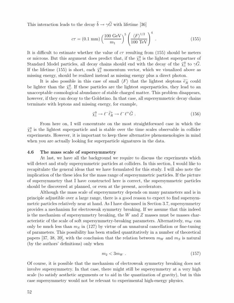
This interaction leads to the decay b → γG with lifetime [36]
cτ = (0.1 mm)(
100 GeV
m1
)5 〈F 〉1/2
100 TeV
4
. (155)
It is difficult to estimate whether the value of cτ resulting from (155) should be metersor microns. But this argument does predict that, if the χ0
1 is the lightest superpartner of
Standard Model particles, all decay chains should end with the decay of the χ01 to γG.
If the lifetime (155) is short, each χ01 momentum vector, which we visualized above as
missing energy, should be realized instead as missing energy plus a direct photon.It is also possible in this case of small 〈F 〉 that the lightest sleptons e−R could
be lighter than the χ01. If these particles are the lightest superparticles, they lead to an
unacceptable cosmological abundance of stable charged matter. This problem disappears,however, if they can decay to the Goldstino. In that case, all supersymmetric decay chains
terminate with leptons and missing energy, for example,
χ01 → ℓ−ℓ+R → ℓ−ℓ+G . (156)
From here on, I will concentrate on the most straightforward case in which theχ0
1 is the lightest superparticle and is stable over the time scales observable in collider
experiments. However, it is important to keep these alternative phenomenologies in mind
when you are actually looking for superparticle signatures in the data.
4.6 The mass scale of supersymmetry
At last, we have all the background we require to discuss the experiments whichwill detect and study supersymmetric particles at colliders. In this section, I would like to
recapitulate the general ideas that we have formulated for this study. I will also note theimplication of the these idea for the mass range of supersymmetric particles. If the picture
of supersymmetry that I have constructed here is correct, the supersymmetric particlesshould be discovered at planned, or even at the present, accelerators.
Although the mass scale of supersymmetry depends on many parameters and is inprinciple adjustible over a large range, there is a good reason to expect to find supersym-
metric particles relatively near at hand. As I have discussed in Section 3.7, supersymmetry
provides a mechanism for electroweak symmetry breaking. If we assume that this indeedis the mechanism of supersymmetry breaking, the W and Z masses must be masses char-
acteristic of the scale of soft supersymmetry-breaking parameters. Alternatively, mW canonly be much less than mS in (127) by virtue of an unnatural cancellation or fine-tuning
of parameters. This possibility has been studied quantitatively in a number of theoreticalpapers [37, 38, 39], with the conclusion that the relation between mW and mS is natural
(by the authors’ definitions) only when
m2 < 3mW . (157)
Of course, it is possible that the mechanism of electroweak symmetry breaking does not
involve supersymmetry. In that case, there might still be supersymmetry at a very highscale (to satisfy aesthetic arguments or to aid in the quantization of gravity), but in this
case supersymmetry would not be relevant to experimental high-energy physics.
52
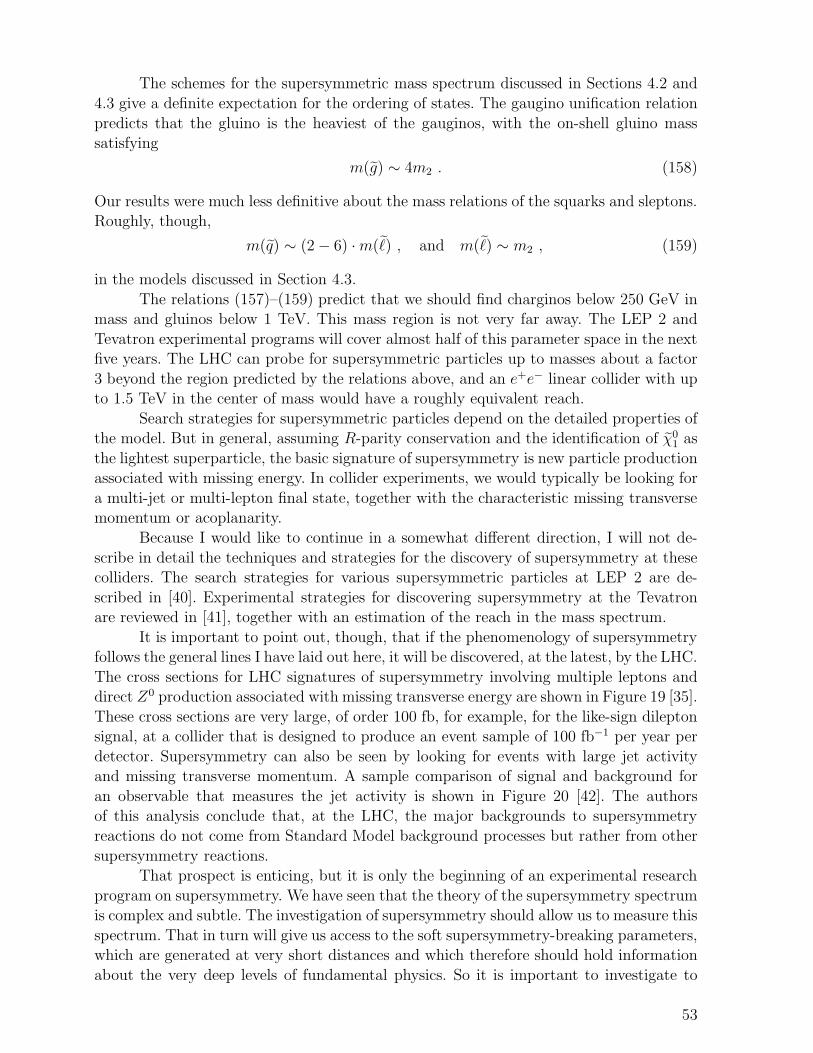
The schemes for the supersymmetric mass spectrum discussed in Sections 4.2 and
4.3 give a definite expectation for the ordering of states. The gaugino unification relation
predicts that the gluino is the heaviest of the gauginos, with the on-shell gluino masssatisfying
m(g) ∼ 4m2 . (158)
Our results were much less definitive about the mass relations of the squarks and sleptons.Roughly, though,
m(q) ∼ (2 − 6) ·m(ℓ) , and m(ℓ) ∼ m2 , (159)
in the models discussed in Section 4.3.
The relations (157)–(159) predict that we should find charginos below 250 GeV inmass and gluinos below 1 TeV. This mass region is not very far away. The LEP 2 and
Tevatron experimental programs will cover almost half of this parameter space in the nextfive years. The LHC can probe for supersymmetric particles up to masses about a factor
3 beyond the region predicted by the relations above, and an e+e− linear collider with upto 1.5 TeV in the center of mass would have a roughly equivalent reach.
Search strategies for supersymmetric particles depend on the detailed properties ofthe model. But in general, assuming R-parity conservation and the identification of χ0
1 as
the lightest superparticle, the basic signature of supersymmetry is new particle productionassociated with missing energy. In collider experiments, we would typically be looking for
a multi-jet or multi-lepton final state, together with the characteristic missing transversemomentum or acoplanarity.
Because I would like to continue in a somewhat different direction, I will not de-
scribe in detail the techniques and strategies for the discovery of supersymmetry at thesecolliders. The search strategies for various supersymmetric particles at LEP 2 are de-
scribed in [40]. Experimental strategies for discovering supersymmetry at the Tevatronare reviewed in [41], together with an estimation of the reach in the mass spectrum.
It is important to point out, though, that if the phenomenology of supersymmetryfollows the general lines I have laid out here, it will be discovered, at the latest, by the LHC.
The cross sections for LHC signatures of supersymmetry involving multiple leptons anddirect Z0 production associated with missing transverse energy are shown in Figure 19 [35].
These cross sections are very large, of order 100 fb, for example, for the like-sign dileptonsignal, at a collider that is designed to produce an event sample of 100 fb−1 per year per
detector. Supersymmetry can also be seen by looking for events with large jet activityand missing transverse momentum. A sample comparison of signal and background for
an observable that measures the jet activity is shown in Figure 20 [42]. The authorsof this analysis conclude that, at the LHC, the major backgrounds to supersymmetry
reactions do not come from Standard Model background processes but rather from other
supersymmetry reactions.That prospect is enticing, but it is only the beginning of an experimental research
program on supersymmetry. We have seen that the theory of the supersymmetry spectrumis complex and subtle. The investigation of supersymmetry should allow us to measure this
spectrum. That in turn will give us access to the soft supersymmetry-breaking parameters,which are generated at very short distances and which therefore should hold information
about the very deep levels of fundamental physics. So it is important to investigate to
53
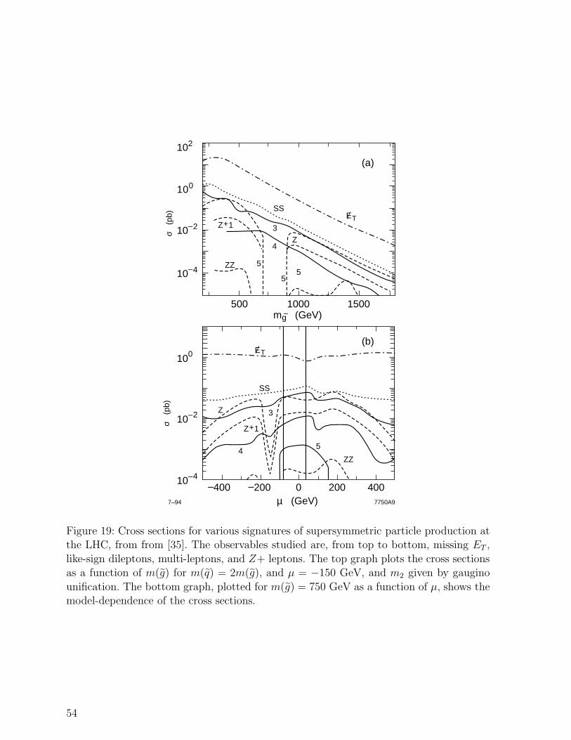
10–4
1000 1500
(a)
mg (GeV)~500
3
SSET
4Z
55
5ZZ
Z+110–2
102
100
σ (
pb)
µ (GeV)–200–400
7–94 7750A9
10–4
4ZZ
5
0 400200
Z+1
3Z
SS
(b)ET
10–2
100
σ (
pb)
Figure 19: Cross sections for various signatures of supersymmetric particle production atthe LHC, from from [35]. The observables studied are, from top to bottom, missing ET ,
like-sign dileptons, multi-leptons, and Z+ leptons. The top graph plots the cross sectionsas a function of m(g) for m(q) = 2m(g), and µ = −150 GeV, and m2 given by gaugino
unification. The bottom graph, plotted for m(g) = 750 GeV as a function of µ, shows themodel-dependence of the cross sections.
54

LHC Point 1
10-13
10-12
10-11
10-10
10-9
10-8
10-7
0 1000 2000 3000 4000Meff (GeV)
dσ
/dM
eff (
mb
/40
0 G
eV
)
Figure 20: Simulation of the observation of supersymmetric particle production at the
LHC, from [42], at a point in parameter space with m(g) = 1 TeV. The observable Meff
is given by the sum of the missing ET and the sum of the ET values for the four hardest
jets. The supersymmetry signal is shown as the open circles. Among the backgrounds, thesquares are due to QCD processes, and the other points shown are due to W , Z, and t
production.
what extent these experimental measurements are actually feasible using accelerators thatwe can foresee.
In discussing this question, I will assume, pessimistically, that the scale of super-symmetry is relatively high, and so I will concentrate on experiments for the high-energy
colliders of the next generation, the LHC and the e+e− linear collider discussed in theintroduction. As a byproduct, this approach will illustrate the deep analytic power that
both of these machines can bring to bear on new physical phenomena.
4.7 Superspectroscopy at e+e− colliders
I will start this discussion of supersymmetry measurements from the side of e+e−
colliders. It is intuitively clear that, if we had an e+e− collider operating in the energyregion appropriate to supersymmetric particle production, some precision measurements
could be made. But I have stressed that the soft supersymmetry-breaking Lagrangiancan contain a very large number of parameters which become intertwined in the mass
spectrum. Thus, it is important to ask, is there a set of measurements which extracts and
55
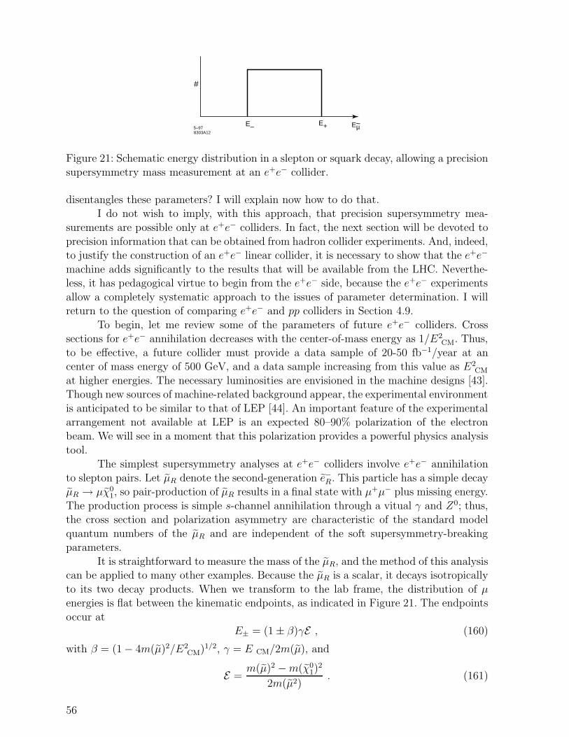
E– Eµ~E+5–978303A12
#
Figure 21: Schematic energy distribution in a slepton or squark decay, allowing a precisionsupersymmetry mass measurement at an e+e− collider.
disentangles these parameters? I will explain now how to do that.I do not wish to imply, with this approach, that precision supersymmetry mea-
surements are possible only at e+e− colliders. In fact, the next section will be devoted to
precision information that can be obtained from hadron collider experiments. And, indeed,to justify the construction of an e+e− linear collider, it is necessary to show that the e+e−
machine adds significantly to the results that will be available from the LHC. Neverthe-less, it has pedagogical virtue to begin from the e+e− side, because the e+e− experiments
allow a completely systematic approach to the issues of parameter determination. I willreturn to the question of comparing e+e− and pp colliders in Section 4.9.
To begin, let me review some of the parameters of future e+e− colliders. Crosssections for e+e− annihilation decreases with the center-of-mass energy as 1/E2
CM. Thus,
to be effective, a future collider must provide a data sample of 20-50 fb−1/year at ancenter of mass energy of 500 GeV, and a data sample increasing from this value as E2
CM
at higher energies. The necessary luminosities are envisioned in the machine designs [43].Though new sources of machine-related background appear, the experimental environment
is anticipated to be similar to that of LEP [44]. An important feature of the experimentalarrangement not available at LEP is an expected 80–90% polarization of the electron
beam. We will see in a moment that this polarization provides a powerful physics analysis
tool.The simplest supersymmetry analyses at e+e− colliders involve e+e− annihilation
to slepton pairs. Let µR denote the second-generation e−R. This particle has a simple decayµR → µχ0
1, so pair-production of µR results in a final state with µ+µ− plus missing energy.
The production process is simple s-channel annihilation through a vitual γ and Z0; thus,the cross section and polarization asymmetry are characteristic of the standard model
quantum numbers of the µR and are independent of the soft supersymmetry-breakingparameters.
It is straightforward to measure the mass of the µR, and the method of this analysiscan be applied to many other examples. Because the µR is a scalar, it decays isotropically
to its two decay products. When we transform to the lab frame, the distribution of µenergies is flat between the kinematic endpoints, as indicated in Figure 21. The endpoints
occur atE± = (1 ± β)γE , (160)
with β = (1 − 4m(µ)2/E2CM)1/2, γ = E CM/2m(µ), and
E =m(µ)2 −m(χ0
1)2
2m(µ2). (161)
56
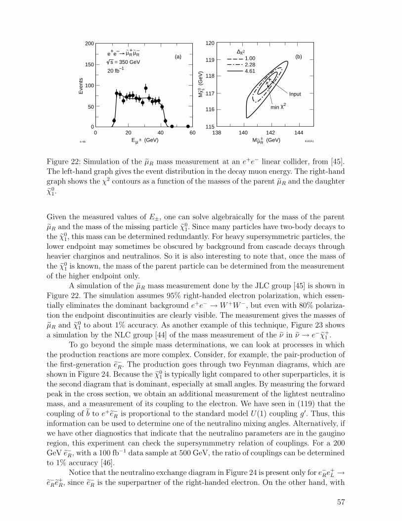
00
119
120
Eve
nts
200
150
(a)R R (b)
Input
min χ2
20 40
117
118
116
115
100
50
60MµR (GeV)
138 140±Eµ (GeV)± ~
142 144
e+e– µ+µ–
s = 350 GeV
20 fb–1
~ ~
Mχ 1 (
GeV
)0
~
∆χ2
1.00 2.28 4.61
8142A14–96
Figure 22: Simulation of the µR mass measurement at an e+e− linear collider, from [45].The left-hand graph gives the event distribution in the decay muon energy. The right-hand
graph shows the χ2 contours as a function of the masses of the parent µR and the daughterχ0
1.
Given the measured values of E±, one can solve algebraically for the mass of the parent
µR and the mass of the missing particle χ01. Since many particles have two-body decays to
the χ01, this mass can be determined redundantly. For heavy supersymmetric particles, the
lower endpoint may sometimes be obscured by background from cascade decays throughheavier charginos and neutralinos. So it is also interesting to note that, once the mass of
the χ01 is known, the mass of the parent particle can be determined from the measurement
of the higher endpoint only.A simulation of the µR mass measurement done by the JLC group [45] is shown in
Figure 22. The simulation assumes 95% right-handed electron polarization, which essen-tially eliminates the dominant background e+e− →W+W−, but even with 80% polariza-
tion the endpoint discontinuities are clearly visible. The measurement gives the masses ofµR and χ0
1 to about 1% accuracy. As another example of this technique, Figure 23 shows
a simulation by the NLC group [44] of the mass measurement of the ν in ν → e−χ+1 .
To go beyond the simple mass determinations, we can look at processes in which
the production reactions are more complex. Consider, for example, the pair-production ofthe first-generation e−R. The production goes through two Feynman diagrams, which are
shown in Figure 24. Because the χ01 is typically light compared to other superparticles, it is
the second diagram that is dominant, especially at small angles. By measuring the forward
peak in the cross section, we obtain an additional measurement of the lightest neutralinomass, and a measurement of its coupling to the electron. We have seen in (119) that the
coupling of b to e+e−R is proportional to the standard model U(1) coupling g′. Thus, this
information can be used to determine one of the neutralino mixing angles. Alternatively, ifwe have other diagnostics that indicate that the neutralino parameters are in the gaugino
region, this experiment can check the supersymmmetry relation of couplings. For a 200GeV e−R, with a 100 fb−1 data sample at 500 GeV, the ratio of couplings can be determined
to 1% accuracy [46].Notice that the neutralino exchange diagram in Figure 24 is present only for e−Re
+L →
e−Re+R, since e−R is the superpartner of the right-handed electron. On the other hand, with
57
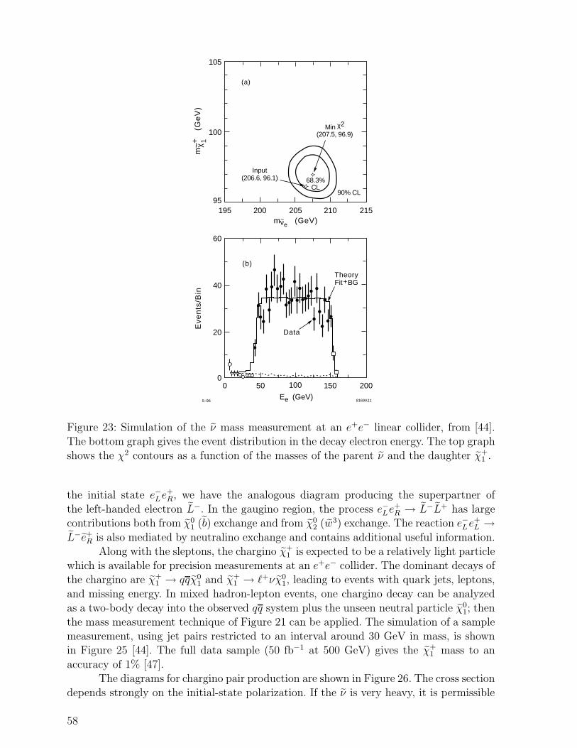
0 100 150 200
Eve
nts
/Bin
Ee (GeV)
0
20
5–96 8169A11
(b)
Theory Fit+BG40
60
100
95
105
50
215210205200195mνe
(GeV)~
(a)
90% CL
68.3% CL
Data
Min χ2 (207.5, 96.9)
Input (206.6, 96.1)
+m
χ 1
(G
eV
)~
Figure 23: Simulation of the ν mass measurement at an e+e− linear collider, from [44].The bottom graph gives the event distribution in the decay electron energy. The top graph
shows the χ2 contours as a function of the masses of the parent ν and the daughter χ+1 .
the initial state e−Le+R, we have the analogous diagram producing the superpartner of
the left-handed electron L−. In the gaugino region, the process e−Le+R → L−L+ has large
contributions both from χ01 (b) exchange and from χ0
2 (w3) exchange. The reaction e−Le+L →
L−e+R is also mediated by neutralino exchange and contains additional useful information.Along with the sleptons, the chargino χ+
1 is expected to be a relatively light particle
which is available for precision measurements at an e+e− collider. The dominant decays ofthe chargino are χ+
1 → qqχ01 and χ+
1 → ℓ+νχ01, leading to events with quark jets, leptons,
and missing energy. In mixed hadron-lepton events, one chargino decay can be analyzed
as a two-body decay into the observed qq system plus the unseen neutral particle χ01; then
the mass measurement technique of Figure 21 can be applied. The simulation of a sample
measurement, using jet pairs restricted to an interval around 30 GeV in mass, is shownin Figure 25 [44]. The full data sample (50 fb−1 at 500 GeV) gives the χ+
1 mass to an
accuracy of 1% [47].The diagrams for chargino pair production are shown in Figure 26. The cross section
depends strongly on the initial-state polarization. If the ν is very heavy, it is permissible
58
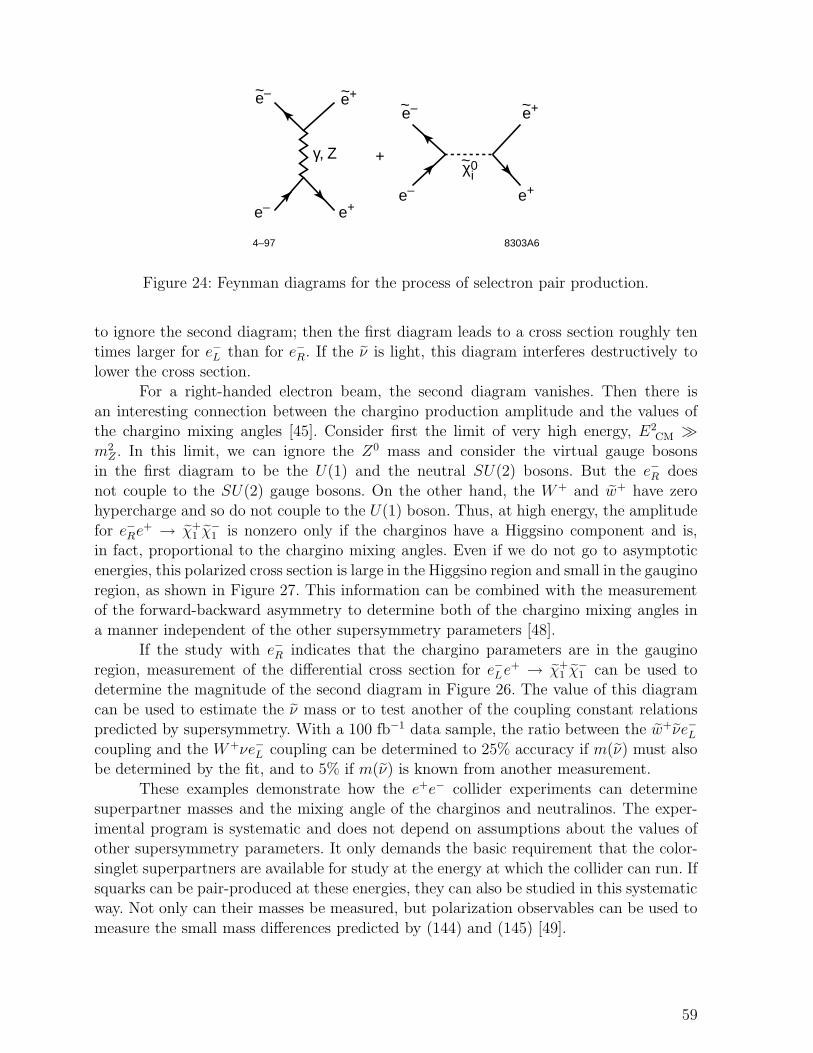
e– e+
e– e+
e– e+
e– e+~ ~
~~
~
4–97
+
8303A6
χi0
γ, Ζ
Figure 24: Feynman diagrams for the process of selectron pair production.
to ignore the second diagram; then the first diagram leads to a cross section roughly tentimes larger for e−L than for e−R. If the ν is light, this diagram interferes destructively to
lower the cross section.For a right-handed electron beam, the second diagram vanishes. Then there is
an interesting connection between the chargino production amplitude and the values ofthe chargino mixing angles [45]. Consider first the limit of very high energy, E2
CM ≫m2Z . In this limit, we can ignore the Z0 mass and consider the virtual gauge bosons
in the first diagram to be the U(1) and the neutral SU(2) bosons. But the e−R does
not couple to the SU(2) gauge bosons. On the other hand, the W+ and w+ have zerohypercharge and so do not couple to the U(1) boson. Thus, at high energy, the amplitude
for e−Re+ → χ+
1 χ−1 is nonzero only if the charginos have a Higgsino component and is,
in fact, proportional to the chargino mixing angles. Even if we do not go to asymptotic
energies, this polarized cross section is large in the Higgsino region and small in the gaugino
region, as shown in Figure 27. This information can be combined with the measurementof the forward-backward asymmetry to determine both of the chargino mixing angles in
a manner independent of the other supersymmetry parameters [48].If the study with e−R indicates that the chargino parameters are in the gaugino
region, measurement of the differential cross section for e−Le+ → χ+
1 χ−1 can be used to
determine the magnitude of the second diagram in Figure 26. The value of this diagram
can be used to estimate the ν mass or to test another of the coupling constant relationspredicted by supersymmetry. With a 100 fb−1 data sample, the ratio between the w+νe−Lcoupling and the W+νe−L coupling can be determined to 25% accuracy if m(ν) must alsobe determined by the fit, and to 5% if m(ν) is known from another measurement.
These examples demonstrate how the e+e− collider experiments can determinesuperpartner masses and the mixing angle of the charginos and neutralinos. The exper-
imental program is systematic and does not depend on assumptions about the values ofother supersymmetry parameters. It only demands the basic requirement that the color-
singlet superpartners are available for study at the energy at which the collider can run. If
squarks can be pair-produced at these energies, they can also be studied in this systematicway. Not only can their masses be measured, but polarization observables can be used to
measure the small mass differences predicted by (144) and (145) [49].
59
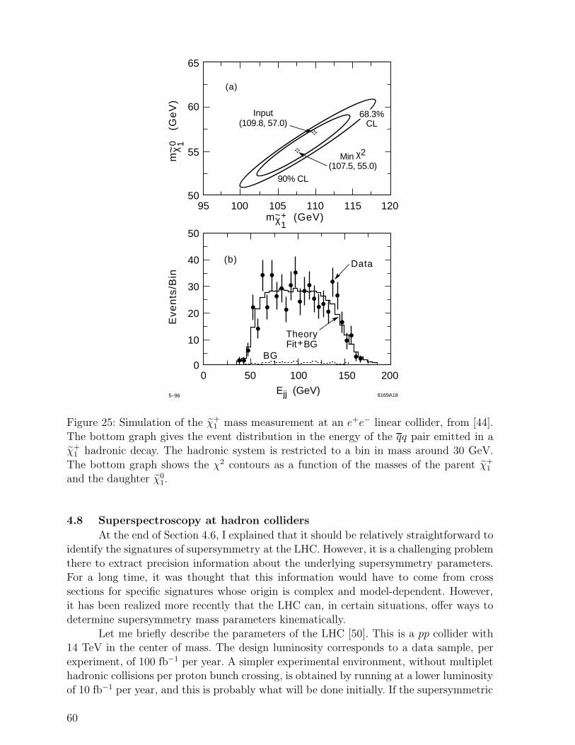
0 50 100 150 200
Eve
nts
/Bin
Ejj (GeV)
0
50
40
30
20
10
5–96 8169A18
(b)
BG
Data
Theory Fit+BG
95 10050
55
60
65
105 110 115 120mχ1
(GeV)~
(a)
90% CL
Min χ2 (107.5, 55.0)
Input (109.8, 57.0)
68.3% CL
0m
χ 1
(G
eV
)~
+
Figure 25: Simulation of the χ+1 mass measurement at an e+e− linear collider, from [44].
The bottom graph gives the event distribution in the energy of the qq pair emitted in aχ+
1 hadronic decay. The hadronic system is restricted to a bin in mass around 30 GeV.
The bottom graph shows the χ2 contours as a function of the masses of the parent χ+1
and the daughter χ01.
4.8 Superspectroscopy at hadron colliders
At the end of Section 4.6, I explained that it should be relatively straightforward toidentify the signatures of supersymmetry at the LHC. However, it is a challenging problem
there to extract precision information about the underlying supersymmetry parameters.For a long time, it was thought that this information would have to come from cross
sections for specific signatures whose origin is complex and model-dependent. However,
it has been realized more recently that the LHC can, in certain situations, offer ways todetermine supersymmetry mass parameters kinematically.
Let me briefly describe the parameters of the LHC [50]. This is a pp collider with14 TeV in the center of mass. The design luminosity corresponds to a data sample, per
experiment, of 100 fb−1 per year. A simpler experimental environment, without multiplethadronic collisions per proton bunch crossing, is obtained by running at a lower luminosity
of 10 fb−1 per year, and this is probably what will be done initially. If the supersymmetric
60
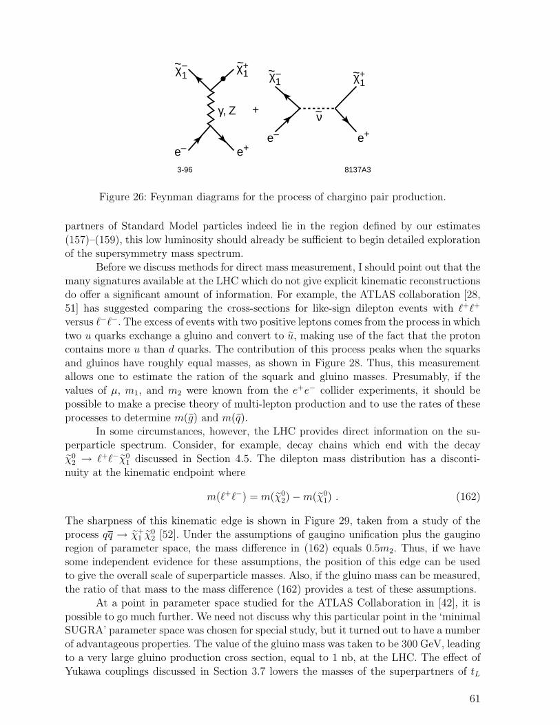
χ1χ1
γ, Ζ ν
e– e+e– e+
χ1– χ1
+– +~ ~
~ ~
~
3-96 8137A3
+
Figure 26: Feynman diagrams for the process of chargino pair production.
partners of Standard Model particles indeed lie in the region defined by our estimates
(157)–(159), this low luminosity should already be sufficient to begin detailed explorationof the supersymmetry mass spectrum.
Before we discuss methods for direct mass measurement, I should point out that the
many signatures available at the LHC which do not give explicit kinematic reconstructionsdo offer a significant amount of information. For example, the ATLAS collaboration [28,
51] has suggested comparing the cross-sections for like-sign dilepton events with ℓ+ℓ+
versus ℓ−ℓ−. The excess of events with two positive leptons comes from the process in which
two u quarks exchange a gluino and convert to u, making use of the fact that the protoncontains more u than d quarks. The contribution of this process peaks when the squarks
and gluinos have roughly equal masses, as shown in Figure 28. Thus, this measurementallows one to estimate the ration of the squark and gluino masses. Presumably, if the
values of µ, m1, and m2 were known from the e+e− collider experiments, it should bepossible to make a precise theory of multi-lepton production and to use the rates of these
processes to determine m(g) and m(q).In some circumstances, however, the LHC provides direct information on the su-
perparticle spectrum. Consider, for example, decay chains which end with the decayχ0
2 → ℓ+ℓ−χ01 discussed in Section 4.5. The dilepton mass distribution has a disconti-
nuity at the kinematic endpoint where
m(ℓ+ℓ−) = m(χ02) −m(χ0
1) . (162)
The sharpness of this kinematic edge is shown in Figure 29, taken from a study of theprocess qq → χ+
1 χ02 [52]. Under the assumptions of gaugino unification plus the gaugino
region of parameter space, the mass difference in (162) equals 0.5m2. Thus, if we havesome independent evidence for these assumptions, the position of this edge can be used
to give the overall scale of superparticle masses. Also, if the gluino mass can be measured,
the ratio of that mass to the mass difference (162) provides a test of these assumptions.At a point in parameter space studied for the ATLAS Collaboration in [42], it is
possible to go much further. We need not discuss why this particular point in the ‘minimalSUGRA’ parameter space was chosen for special study, but it turned out to have a number
of advantageous properties. The value of the gluino mass was taken to be 300 GeV, leadingto a very large gluino production cross section, equal to 1 nb, at the LHC. The effect of
Yukawa couplings discussed in Section 3.7 lowers the masses of the superpartners of tL
61
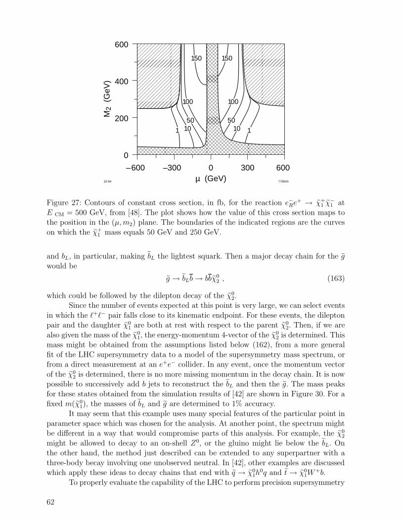
������–600 –300 0 300
0
200
400
600
µ (GeV)
M2
(G
eV)
600
10 10
100 100
150 150
50
1
10-94
7790A5
������ ������������ 1
50
Figure 27: Contours of constant cross section, in fb, for the reaction e−Re+ → χ+
1 χ−1 at
E CM = 500 GeV, from [48]. The plot shows how the value of this cross section maps tothe position in the (µ,m2) plane. The boundaries of the indicated regions are the curves
on which the χ+1 mass equals 50 GeV and 250 GeV.
and bL, in particular, making bL the lightest squark. Then a major decay chain for the g
would be
g → bLb→ bbχ02 , (163)
which could be followed by the dilepton decay of the χ02.
Since the number of events expected at this point is very large, we can select events
in which the ℓ+ℓ− pair falls close to its kinematic endpoint. For these events, the dileptonpair and the daughter χ0
1 are both at rest with respect to the parent χ02. Then, if we are
also given the mass of the χ01, the energy-momentum 4-vector of the χ0
2 is determined. Thismass might be obtained from the assumptions listed below (162), from a more general
fit of the LHC supersymmetry data to a model of the supersymmetry mass spectrum, orfrom a direct measurement at an e+e− collider. In any event, once the momentum vector
of the χ02 is determined, there is no more missing momentum in the decay chain. It is now
possible to successively add b jets to reconstruct the bL and then the g. The mass peaks
for these states obtained from the simulation results of [42] are shown in Figure 30. For afixed m(χ0
1), the masses of bL and g are determined to 1% accuracy.
It may seem that this example uses many special features of the particular point in
parameter space which was chosen for the analysis. At another point, the spectrum mightbe different in a way that would compromise parts of this analysis. For example, the χ0
2
might be allowed to decay to an on-shell Z0, or the gluino might lie below the bL. Onthe other hand, the method just described can be extended to any superpartner with a
three-body becay involving one unobserved neutral. In [42], other examples are discussedwhich apply these ideas to decay chains that end with q → χ0
1h0q and t→ χ0
1W+b.
To properly evaluate the capability of the LHC to perform precision supersymmetry
62
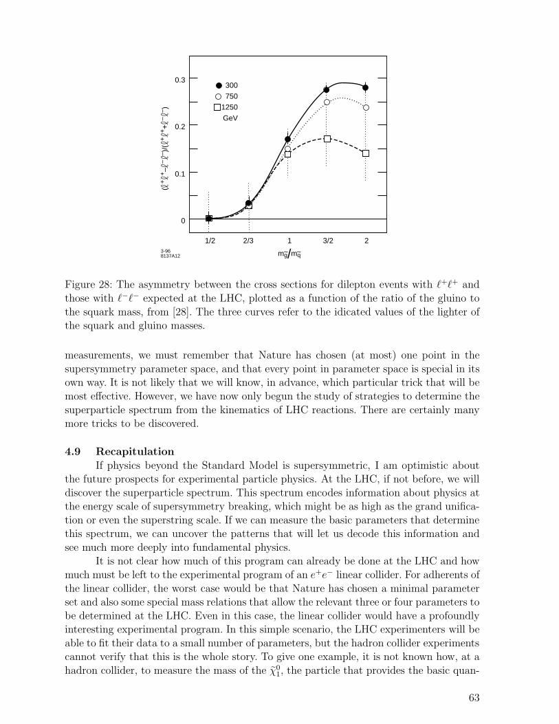
1/2
0
0.1
0.2
300
750
1250
GeV
0.3
2/3 1 23/2
mg/mq~ ~
( +
+–
– –
)/(
+ +
+ –
–)
3-96 8137A12
Figure 28: The asymmetry between the cross sections for dilepton events with ℓ+ℓ+ and
those with ℓ−ℓ− expected at the LHC, plotted as a function of the ratio of the gluino to
the squark mass, from [28]. The three curves refer to the idicated values of the lighter ofthe squark and gluino masses.
measurements, we must remember that Nature has chosen (at most) one point in the
supersymmetry parameter space, and that every point in parameter space is special in itsown way. It is not likely that we will know, in advance, which particular trick that will be
most effective. However, we have now only begun the study of strategies to determine the
superparticle spectrum from the kinematics of LHC reactions. There are certainly manymore tricks to be discovered.
4.9 Recapitulation
If physics beyond the Standard Model is supersymmetric, I am optimistic aboutthe future prospects for experimental particle physics. At the LHC, if not before, we will
discover the superparticle spectrum. This spectrum encodes information about physics atthe energy scale of supersymmetry breaking, which might be as high as the grand unifica-
tion or even the superstring scale. If we can measure the basic parameters that determinethis spectrum, we can uncover the patterns that will let us decode this information and
see much more deeply into fundamental physics.It is not clear how much of this program can already be done at the LHC and how
much must be left to the experimental program of an e+e− linear collider. For adherents of
the linear collider, the worst case would be that Nature has chosen a minimal parameterset and also some special mass relations that allow the relevant three or four parameters to
be determined at the LHC. Even in this case, the linear collider would have a profoundlyinteresting experimental program. In this simple scenario, the LHC experimenters will be
able to fit their data to a small number of parameters, but the hadron collider experimentscannot verify that this is the whole story. To give one example, it is not known how, at a
hadron collider, to measure the mass of the χ01, the particle that provides the basic quan-
63
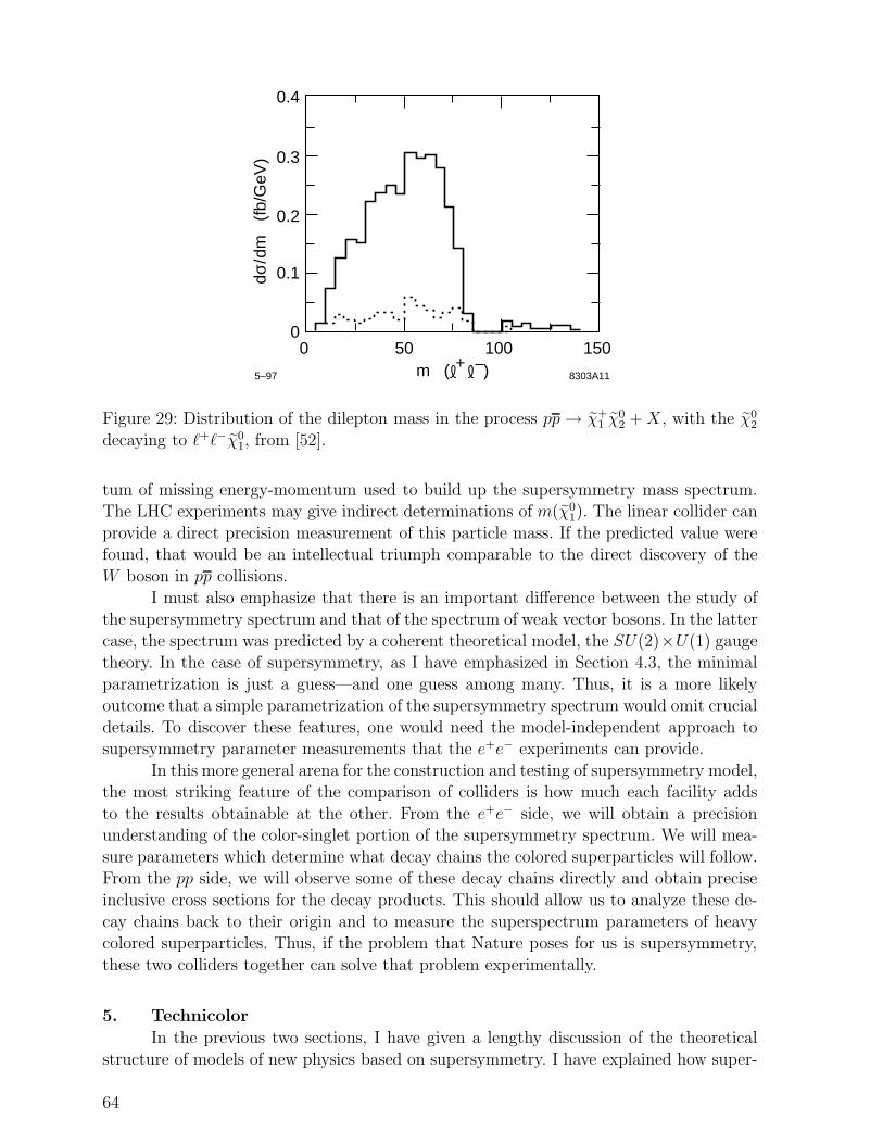
0 50 100 1500
0.2
0.1
0.4
0.3
m ( + –)
dσ/d
m
(fb/
GeV
)
5–97 8303A11
Figure 29: Distribution of the dilepton mass in the process pp→ χ+1 χ
02 +X, with the χ0
2
decaying to ℓ+ℓ−χ01, from [52].
tum of missing energy-momentum used to build up the supersymmetry mass spectrum.The LHC experiments may give indirect determinations of m(χ0
1). The linear collider can
provide a direct precision measurement of this particle mass. If the predicted value werefound, that would be an intellectual triumph comparable to the direct discovery of the
W boson in pp collisions.
I must also emphasize that there is an important difference between the study ofthe supersymmetry spectrum and that of the spectrum of weak vector bosons. In the latter
case, the spectrum was predicted by a coherent theoretical model, the SU(2)×U(1) gaugetheory. In the case of supersymmetry, as I have emphasized in Section 4.3, the minimal
parametrization is just a guess—and one guess among many. Thus, it is a more likelyoutcome that a simple parametrization of the supersymmetry spectrum would omit crucial
details. To discover these features, one would need the model-independent approach tosupersymmetry parameter measurements that the e+e− experiments can provide.
In this more general arena for the construction and testing of supersymmetry model,the most striking feature of the comparison of colliders is how much each facility adds
to the results obtainable at the other. From the e+e− side, we will obtain a precisionunderstanding of the color-singlet portion of the supersymmetry spectrum. We will mea-
sure parameters which determine what decay chains the colored superparticles will follow.From the pp side, we will observe some of these decay chains directly and obtain precise
inclusive cross sections for the decay products. This should allow us to analyze these de-
cay chains back to their origin and to measure the superspectrum parameters of heavycolored superparticles. Thus, if the problem that Nature poses for us is supersymmetry,
these two colliders together can solve that problem experimentally.
5. Technicolor
In the previous two sections, I have given a lengthy discussion of the theoretical
structure of models of new physics based on supersymmetry. I have explained how super-
64
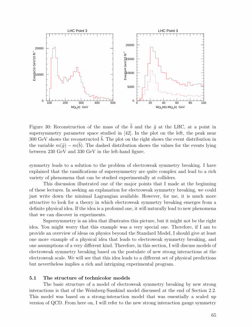
LHC Point 3
0
10000
20000
100 200 300 400 500M(χ2b) GeV
Eve
nts/
10 G
eV/1
0 fb
-1LHC Point 3
0
5000
10000
15000
20000
0 20 40 60 80 100M(χ2bb)-M(χ2b) GeV
Eve
nts/
4 G
eV/1
0 fb
-1
Figure 30: Reconstruction of the mass of the b and the g at the LHC, at a point in
supersymmetry parameter space studied in [42]. In the plot on the left, the peak near300 GeV shows the reconstructed b. The plot on the right shows the event distribution in
the variable m(g) −m(b). The dashed distribution shows the values for the events lyingbetween 230 GeV and 330 GeV in the left-hand figure.
symmetry leads to a solution to the problem of electroweak symmetry breaking. I haveexplained that the ramifications of supersymmetry are quite complex and lead to a rich
variety of phenomena that can be studied experimentally at colliders.This discussion illustrated one of the major points that I made at the beginning
of these lectures. In seeking an explanation for electroweak symmetry breaking, we couldjust write down the minimal Lagrangian available. However, for me, it is much more
attractive to look for a theory in which electroweak symmetry breaking emerges from adefinite physical idea. If the idea is a profound one, it will naturally lead to new phenomena
that we can discover in experiments.Supersymmetry is an idea that illustrates this picture, but it might not be the right
idea. You might worry that this example was a very special one. Therefore, if I am toprovide an overview of ideas on physics beyond the Standard Model, I should give at least
one more example of a physical idea that leads to electroweak symmetry breaking, andone assumptions of a very different kind. Therefore, in this section, I will discuss models of
electroweak symmetry breaking based on the postulate of new strong interactions at the
electroweak scale. We will see that this idea leads to a different set of physical predictionsbut nevertheless implies a rich and intriguing experimental program.
5.1 The structure of technicolor models
The basic structure of a model of electroweak symmetry breaking by new strong
interactions is that of the Weinberg-Susskind model discussed at the end of Section 2.2.This model was based on a strong-interaction model that was essentially a scaled up
version of QCD. From here on, I will refer to the new strong interaction gauge symmetry
65
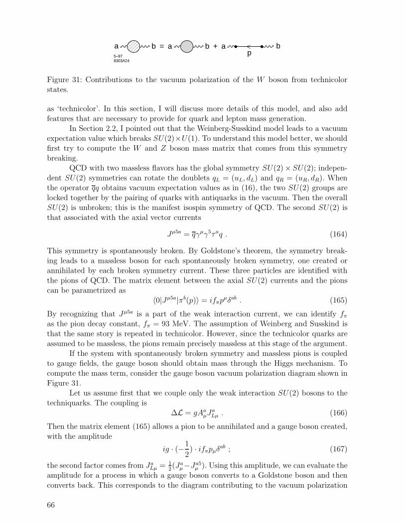
�ya bp5–97
8303A24
b = a b + a
Figure 31: Contributions to the vacuum polarization of the W boson from technicolorstates.
as ‘technicolor’. In this section, I will discuss more details of this model, and also add
features that are necessary to provide for quark and lepton mass generation.In Section 2.2, I pointed out that the Weinberg-Susskind model leads to a vacuum
expectation value which breaks SU(2)×U(1). To understand this model better, we shouldfirst try to compute the W and Z boson mass matrix that comes from this symmetry
breaking.QCD with two massless flavors has the global symmetry SU(2)× SU(2); indepen-
dent SU(2) symmetries can rotate the doublets qL = (uL, dL) and qR = (uR, dR). Whenthe operator qq obtains vacuum expectation values as in (16), the two SU(2) groups are
locked together by the pairing of quarks with antiquarks in the vacuum. Then the overallSU(2) is unbroken; this is the manifest isospin symmetry of QCD. The second SU(2) is
that associated with the axial vector currents
Jµ5a = qγµγ5τaq . (164)
This symmetry is spontaneously broken. By Goldstone’s theorem, the symmetry break-
ing leads to a massless boson for each spontaneously broken symmetry, one created orannihilated by each broken symmetry current. These three particles are identified with
the pions of QCD. The matrix element between the axial SU(2) currents and the pionscan be parametrized as
〈0|Jµ5a|πb(p)〉 = ifπpµδab . (165)
By recognizing that Jµ5a is a part of the weak interaction current, we can identify fπas the pion decay constant, fπ = 93 MeV. The assumption of Weinberg and Susskind is
that the same story is repeated in technicolor. However, since the technicolor quarks are
assumed to be massless, the pions remain precisely massless at this stage of the argument.If the system with spontaneously broken symmetry and massless pions is coupled
to gauge fields, the gauge boson should obtain mass through the Higgs mechanism. Tocompute the mass term, consider the gauge boson vacuum polarization diagram shown in
Figure 31.Let us assume first that we couple only the weak interaction SU(2) bosons to the
techniquarks. The coupling is∆L = gAaµJ
aLµ . (166)
Then the matrix element (165) allows a pion to be annihilated and a gauge boson created,
with the amplitude
ig · (−1
2) · ifπpµδab ; (167)
the second factor comes from JaLµ = 12(Jaµ−Ja5µ ). Using this amplitude, we can evaluate the
amplitude for a process in which a gauge boson converts to a Goldstone boson and then
converts back. This corresponds to the diagram contributing to the vacuum polarization
66
shown as the second term on the right-hand side of Figure 31. The value of this diagram
is (gfπpµ
2
)1
p2
(−gfπpν
2
). (168)
The full vacuum polarization amplitude iΠabµν(p) consists of this term plus more compli-
cated terms with massive particles or multiple particles exchanged. These are indicated asthe shaded blob in Figure 31. If there are no massless particles in the symmetry-breaking
sector other than the pions, (168) is the only term with a 1/p2 singularity near p = 0.Now recognize that the gauge current JaLµ is conserved, and so the vacuum polarization
must satisfy
pµ Πabµν(p) = 0 . (169)
These two requirements are compatible only if the vacuum polarization behaves near p = 0as
Πabµν =
(gfπ2
)2 (gµν −
pµpνp2
)δab . (170)
This is a mass term for the vector boson, giving
mW = gv
2, with v = fπ . (171)
This is the result that I promised above (18).
Now add to this structure the U(1) gauge boson Bµ coupling to hypercharge. Re-peating the same arguments, we find the mass matrix
m2 =
(fπ2
)2
g2
g2
g2 −gg′−gg′ (g′)2
, (172)
acting on (A1µ, A
2µ, A
3µ, Bµ). This has just the form of (21). The eigenvalues of this matrix
give the vector boson masses (7), with v = 246 GeV = fπ. This is the result promised
above (18). More generally, in a model with ND technicolor doublets, we require,
v2 = NDf2π . (173)
Thus, a larger technicolor sector lies lower in energy and is closer to the scale of presentexperiments.
In my discussion of (21), I pointed out that this equation calls for the presenceof an unbroken SU(2) global symmetry of the new strong interactions, called custodial
SU(2), in addition to the spontaneously broken weak interaction SU(2) symmetry. This
global SU(2) symmetry requires that the first three diagonal entries in (172) are equal,giving the mass relation mW/mZ = cos θw. Custodial SU(2) symmetry also acts on the
heavier states of the new strong interaction theory and will play an important role in ouranalysis of the experimental probes of this sector.
The model I have just described gives mass the the W and Z bosons, but it doesnot yet give mass to quarks and leptons. In order to accomplish this, we must couple the
quarks and leptons to the techniquarks. This is done by introducing further gauge bosons
67
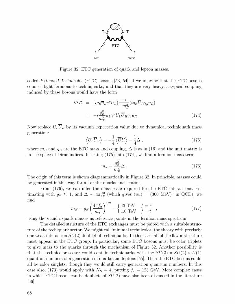
1–97 8267A6
ETC
f f
TT�yFigure 32: ETC generation of quark and lepton masses.
called Extended Technicolor (ETC) bosons [53, 54]. If we imagine that the ETC bosons
connect light fermions to techniquarks, and that they are very heavy, a typical coupling
induced by these bosons would have the form
i∆L = (igEuLγµUL)
−i−m2
E
(igEURγµuR)
= −i g2E
m2E
uLγµULURγµuR (174)
Now replace ULUR by its vacuum expectation value due to dynamical techniquark mass
generation:⟨ULUR
⟩= −1
4
⟨UU
⟩=
1
4∆ , (175)
where mE and gE are the ETC mass and coupling, ∆ is as in (16) and the unit matrix is
in the space of Dirac indices. Inserting (175) into (174), we find a fermion mass term
mu =g2E
m2E
∆ . (176)
The origin of this term is shown diagrammatically in Figure 32. In principle, masses couldbe generated in this way for all of the quarks and leptons.
From (176), we can infer the mass scale required for the ETC interactions. Es-timating with gE ≈ 1, and ∆ ∼ 4πf 3
π (which gives 〈uu〉 = (300 MeV)3 in QCD), we
find
mE = gE
(4πf 3
π
mf
)1/2
={
43 TeV f = s1.0 TeV f = t
, (177)
using the s and t quark masses as reference points in the fermion mass spectrum.The detailed structure of the ETC exchanges must be paired with a suitable struc-
ture of the techiquark sector. We might call ‘minimal technicolor’ the theory with preciselyone weak interaction SU(2) doublet of techniquarks. In this case, all of the flavor structure
must appear in the ETC group. In particular, some ETC bosons must be color triplets
to give mass to the quarks through the mechanism of Figure 32. Another possibility isthat the technicolor sector could contain techniquarks with the SU(3) × SU(2) × U(1)
quantum numbers of a generation of quarks and leptons [55]. Then the ETC bosons couldall be color singlets, though they would still carry generation quantum numbers. In this
case also, (173) would apply with ND = 4, putting fπ = 123 GeV. More complex casesin which ETC bosons can be doublets of SU(2) have also been discussed in the literature
[56].
68
5.2 Experimental constraints on technicolor
The model that I have just described makes a number of characteristic physicalpredictions that can be checked in experiments at energies currently available. Unfortu-
nately, none of these predictions checks experimentally. Many theorists view this as arepudiation of the technicolor program. However, others point to the fact that we have
built up the technicolor model assuming that the dynamics of the technicolor interactionsexactly copies that of QCD. By modifying the pattern or the explicit energy scale of chiral
symmetry breaking, it is possible to evade these difficulties. Nevertheless, it is importantto be aware of what the problems are. In this section, I will review the three major ex-
perimental problems with technicolor models and then briefly examine how they may beavoided through specific assumptions about the strong interaction dynamics.
The first two problems are not specifically associated with technicolor but ratherwith the ETC interactions that couple techniquarks to the Standard Model quarks and
leptons. If two matrices of the ETC group link quarks with techniquarks, the commutatorof these matrices should link quarks with quarks. This implies that there should be ETC
bosons which create new four-quark interactions with coefficients of order g2E/m
2E. In the
Standard Model, there are no flavor-changing neutral current couplings at the tree level.Such couplings are generated by weak interaction box diagrams and other loop effects,
but the flavor-changing part of these interactions is suppressed to the level observedexperimentally by the GIM cancellation among intermediate flavors [57]. This cancellation
follows from the fact that the couplings of the various flavors of quarks and leptons tothe W and Z depend only on their SU(2) × U(1) quantum numbers. For ETC, however,
either the couplings or the boson masses must depend strongly on flavor in order togenerate the observed pattern of quark and lepton masses. Thus, generically, one expects
large flavor-changing neutral current effects. It is possible to suppress these couplings to alevel at which they do not contribute excessively to the KL–KS mass difference, but only
by raising the ETC mass scale to mE ≥ 1000 TeV. In a similar way, ETC interactionsgenerically give excessive contributions to K0 → µ+e− and to µ → eγ unless mE ≥ 100
TeV [58, 59]. These estimates contradict the value of the ETC boson masses required in(177). There are schemes for natural flavor conservation in technicolor theories, but they
require a very large amount of new structure just above 1 TeV [60, 61, 62].
The second problem comes in the value of the top quark mass. If ETC is weaklycoupled, the value of any quark mass should be bounded by approximately
mf ≤g2E
4π∆1/2 , (178)
where ∆ is the techniquark bilinear expectation value. Estimating as above, this boundsthe quark masses at about 70 GeV [63]. To see this problem from another point of view,
look back at the mass of the ETC boson associated with the top quark, as given in (177).
This is comparable to the mass of the technicolor ρ meson, which we would estimate from(18) to have a value of about 2 TeV. So apparently the top quark’s ETC boson must be a
particle with technicolor strong interactions. This means that the model described aboveis not self-consistent. Since this new strongly-interacting particle generates mass for the
t but not the b, it has the potential to give large contributions to other relations thatviolate weak-interaction isospin. In particular, it can give an unwanted large correction
to the relation mW = mZ cos θw in (20).
69
The third problem relates directly to the technicolor sector itself. This issue arises
from the precision electroweak measurments. In principle, the agreement of precision
electroweak measurements with the Standard Model is a strong constraint on any type ofnew physics. The constraint turns out to be especially powerful for technicolor. To explain
this point, I would like to present some general formalism and then specialize it to thecase of technicolor.
At first sight, new physics can affect the observables of precision electroweak physicsthrough radiative corrections to the SU(2)×U(1) boson propagators, to the gauge boson
vertices, and to 4-fermion box diagrams. Typically, though, the largest effects are thosefrom vacuum polarization diagrams. To see this, recall that almost all precision elec-
troweak observables involve 4-fermion reactions with light fermions only. (An exceptionis the Z → bb vertex, whose discussion I will postpone to Section 5.7.) In this case, the
vertex and box diagrams involve only those new particles that couple directly to the lightgenerations. If the new particles are somehow connected to the mechanism of SU(2)×U(1)
breaking and fermion mass generation, these couplings are necessarily small. The vacuumpolarization diagrams, on the other hand, can involve all new particles which couple to
SU(2) × U(1), and can even be enhanced by color or flavor sums over these particles.
The vacuum polarization corrections also can be accounted in a very simple way.It is useful, first, to write the W and Z vacuum polarization amplitudes in terms of
current-current expectation values for the SU(2) and electromagnetic currents. Use therelation
JZ = J3 − s2JQ , (179)
where JQ is the electromagnetic current, and s2 = sin2 θw, c2 = cos2 θw. Write the weak
coupling constants explicitly in terms of e, s2 and c2. Then the vacuum polarizationamplitudes of γ, W , and Z and the γZ mixing amplitude take the form
Πγγ = e2ΠQQ
ΠWW =e2
s2ΠQQ
ΠZZ =e2
c2s2(Π33 − 2s2Π3Q + s4ΠQQ)
ΠZγ =e2
cs(Π3Q − s2ΠQQ) . (180)
The current-current amplitudes Πij are functions of (q2/M2), where M is the mass of the
new particles whose loops contribute to the vacuum polarizations.If these new particles are too heavy to be found at the Z0 or in the early stages
of LEP 2, the ratio q2/M2 is bounded for q2 = m2Z . Then it is reasonable to expand
the current-current expectation values a power series. In making this expansion, it is
important to take into account that any amplitude involving an electromagnetic currentwill vanish at q2 = 0 by the standard QED Ward identity. Thus, to order q2, we have six
coefficients,
ΠQQ = q2Π′QQ(0) + · · ·
Π11 = Π11(0) + q2Π′11(0) + · · ·
Π3Q = q2Π′3Q(0) + · · ·
Π33 = Π33(0) + q2Π′33(0) + · · · (181)
70
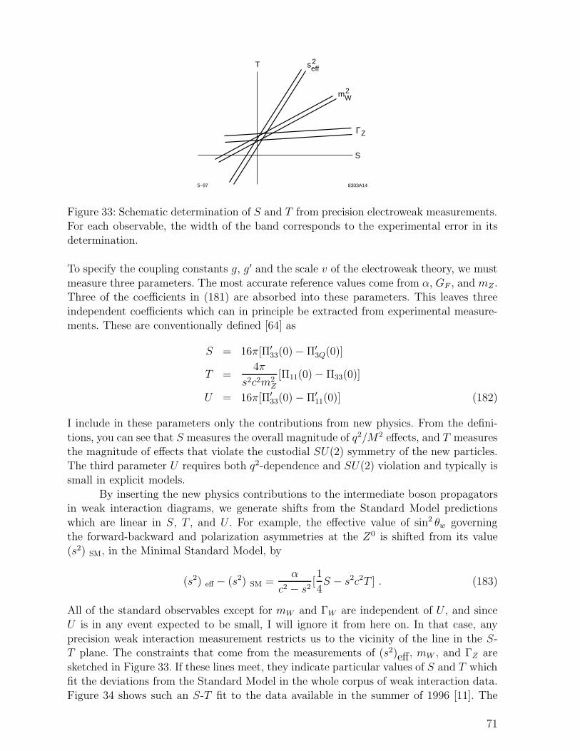
S
T
ΓZ
5–97 8303A14
mW2
seff2
Figure 33: Schematic determination of S and T from precision electroweak measurements.For each observable, the width of the band corresponds to the experimental error in its
determination.
To specify the coupling constants g, g′ and the scale v of the electroweak theory, we must
measure three parameters. The most accurate reference values come from α, GF , and mZ .Three of the coefficients in (181) are absorbed into these parameters. This leaves three
independent coefficients which can in principle be extracted from experimental measure-ments. These are conventionally defined [64] as
S = 16π[Π′33(0) − Π′
3Q(0)]
T =4π
s2c2m2Z
[Π11(0) − Π33(0)]
U = 16π[Π′33(0) − Π′
11(0)] (182)
I include in these parameters only the contributions from new physics. From the defini-
tions, you can see that S measures the overall magnitude of q2/M2 effects, and T measuresthe magnitude of effects that violate the custodial SU(2) symmetry of the new particles.
The third parameter U requires both q2-dependence and SU(2) violation and typically issmall in explicit models.
By inserting the new physics contributions to the intermediate boson propagatorsin weak interaction diagrams, we generate shifts from the Standard Model predictions
which are linear in S, T , and U . For example, the effective value of sin2 θw governingthe forward-backward and polarization asymmetries at the Z0 is shifted from its value
(s2) SM, in the Minimal Standard Model, by
(s2) eff − (s2) SM =α
c2 − s2[1
4S − s2c2T ] . (183)
All of the standard observables except for mW and ΓW are independent of U , and sinceU is in any event expected to be small, I will ignore it from here on. In that case, any
precision weak interaction measurement restricts us to the vicinity of the line in the S-T plane. The constraints that come from the measurements of (s2)eff, mW , and ΓZ are
sketched in Figure 33. If these lines meet, they indicate particular values of S and T whichfit the deviations from the Standard Model in the whole corpus of weak interaction data.
Figure 34 shows such an S-T fit to the data available in the summer of 1996 [11]. The
71
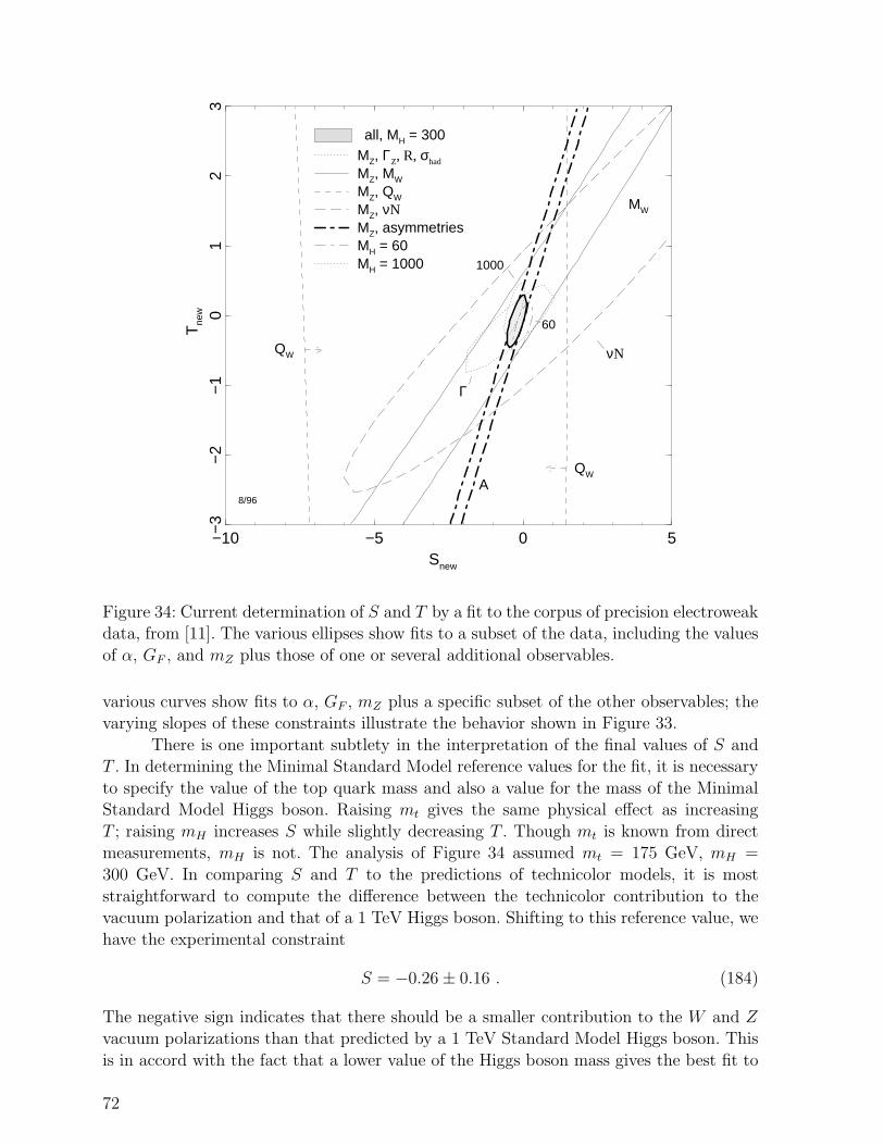
−10 −5 0 5Snew
−3
−2
−1
01
23
Tne
w
MZ, ΓZ, R, σhad
MZ, MW
MZ, QW
MZ, νNMZ, asymmetriesMH = 60MH = 1000
all, MH = 300
νN
QW
QW
Γ
60
1000
MW
A8/96
Figure 34: Current determination of S and T by a fit to the corpus of precision electroweakdata, from [11]. The various ellipses show fits to a subset of the data, including the values
of α, GF , and mZ plus those of one or several additional observables.
various curves show fits to α, GF , mZ plus a specific subset of the other observables; thevarying slopes of these constraints illustrate the behavior shown in Figure 33.
There is one important subtlety in the interpretation of the final values of S andT . In determining the Minimal Standard Model reference values for the fit, it is necessary
to specify the value of the top quark mass and also a value for the mass of the MinimalStandard Model Higgs boson. Raising mt gives the same physical effect as increasing
T ; raising mH increases S while slightly decreasing T . Though mt is known from directmeasurements, mH is not. The analysis of Figure 34 assumed mt = 175 GeV, mH =
300 GeV. In comparing S and T to the predictions of technicolor models, it is most
straightforward to compute the difference between the technicolor contribution to thevacuum polarization and that of a 1 TeV Higgs boson. Shifting to this reference value, we
have the experimental constraint
S = −0.26 ± 0.16 . (184)
The negative sign indicates that there should be a smaller contribution to the W and Zvacuum polarizations than that predicted by a 1 TeV Standard Model Higgs boson. This
is in accord with the fact that a lower value of the Higgs boson mass gives the best fit to
72
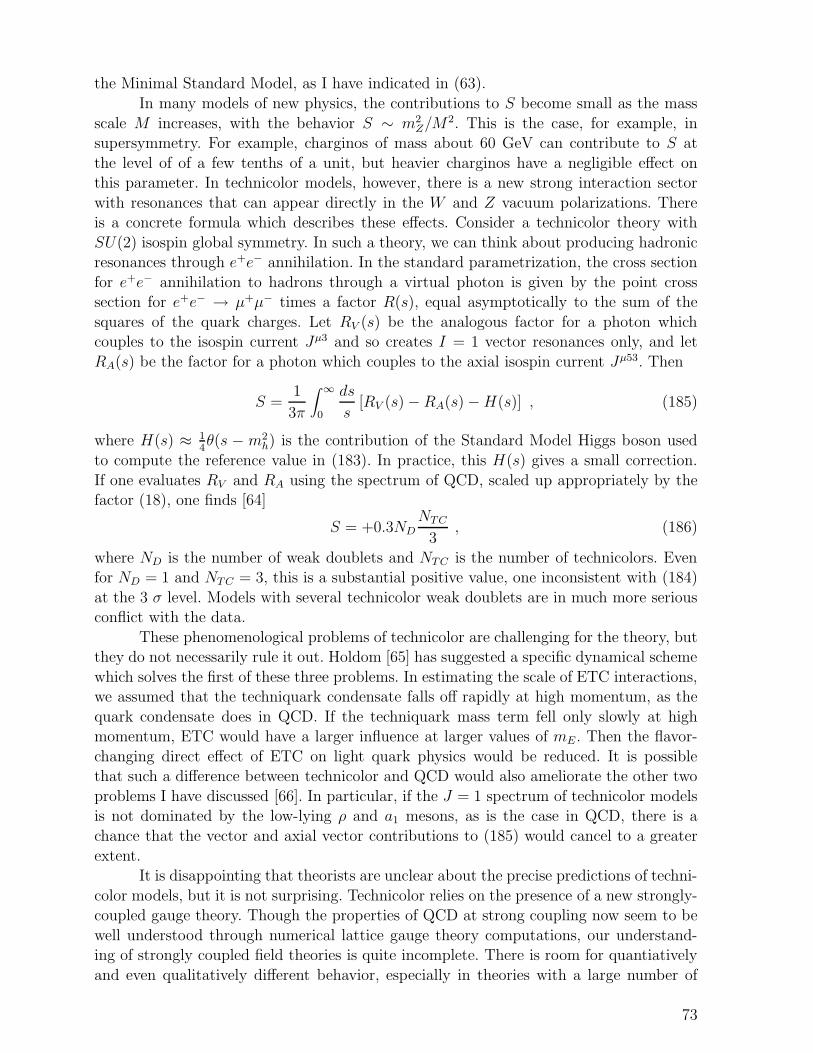
the Minimal Standard Model, as I have indicated in (63).
In many models of new physics, the contributions to S become small as the mass
scale M increases, with the behavior S ∼ m2Z/M
2. This is the case, for example, insupersymmetry. For example, charginos of mass about 60 GeV can contribute to S at
the level of of a few tenths of a unit, but heavier charginos have a negligible effect onthis parameter. In technicolor models, however, there is a new strong interaction sector
with resonances that can appear directly in the W and Z vacuum polarizations. Thereis a concrete formula which describes these effects. Consider a technicolor theory with
SU(2) isospin global symmetry. In such a theory, we can think about producing hadronicresonances through e+e− annihilation. In the standard parametrization, the cross section
for e+e− annihilation to hadrons through a virtual photon is given by the point crosssection for e+e− → µ+µ− times a factor R(s), equal asymptotically to the sum of the
squares of the quark charges. Let RV (s) be the analogous factor for a photon whichcouples to the isospin current Jµ3 and so creates I = 1 vector resonances only, and let
RA(s) be the factor for a photon which couples to the axial isospin current Jµ53. Then
S =1
3π
∫ ∞
0
ds
s[RV (s) − RA(s) −H(s)] , (185)
where H(s) ≈ 14θ(s − m2
h) is the contribution of the Standard Model Higgs boson used
to compute the reference value in (183). In practice, this H(s) gives a small correction.
If one evaluates RV and RA using the spectrum of QCD, scaled up appropriately by thefactor (18), one finds [64]
S = +0.3NDNTC
3, (186)
where ND is the number of weak doublets and NTC is the number of technicolors. Evenfor ND = 1 and NTC = 3, this is a substantial positive value, one inconsistent with (184)
at the 3 σ level. Models with several technicolor weak doublets are in much more seriousconflict with the data.
These phenomenological problems of technicolor are challenging for the theory, butthey do not necessarily rule it out. Holdom [65] has suggested a specific dynamical scheme
which solves the first of these three problems. In estimating the scale of ETC interactions,we assumed that the techniquark condensate falls off rapidly at high momentum, as the
quark condensate does in QCD. If the techniquark mass term fell only slowly at highmomentum, ETC would have a larger influence at larger values of mE . Then the flavor-
changing direct effect of ETC on light quark physics would be reduced. It is possiblethat such a difference between technicolor and QCD would also ameliorate the other two
problems I have discussed [66]. In particular, if the J = 1 spectrum of technicolor modelsis not dominated by the low-lying ρ and a1 mesons, as is the case in QCD, there is a
chance that the vector and axial vector contributions to (185) would cancel to a greater
extent.It is disappointing that theorists are unclear about the precise predictions of techni-
color models, but it is not surprising. Technicolor relies on the presence of a new strongly-coupled gauge theory. Though the properties of QCD at strong coupling now seem to be
well understood through numerical lattice gauge theory computations, our understand-ing of strongly coupled field theories is quite incomplete. There is room for quantiatively
and even qualitatively different behavior, especially in theories with a large number of
73
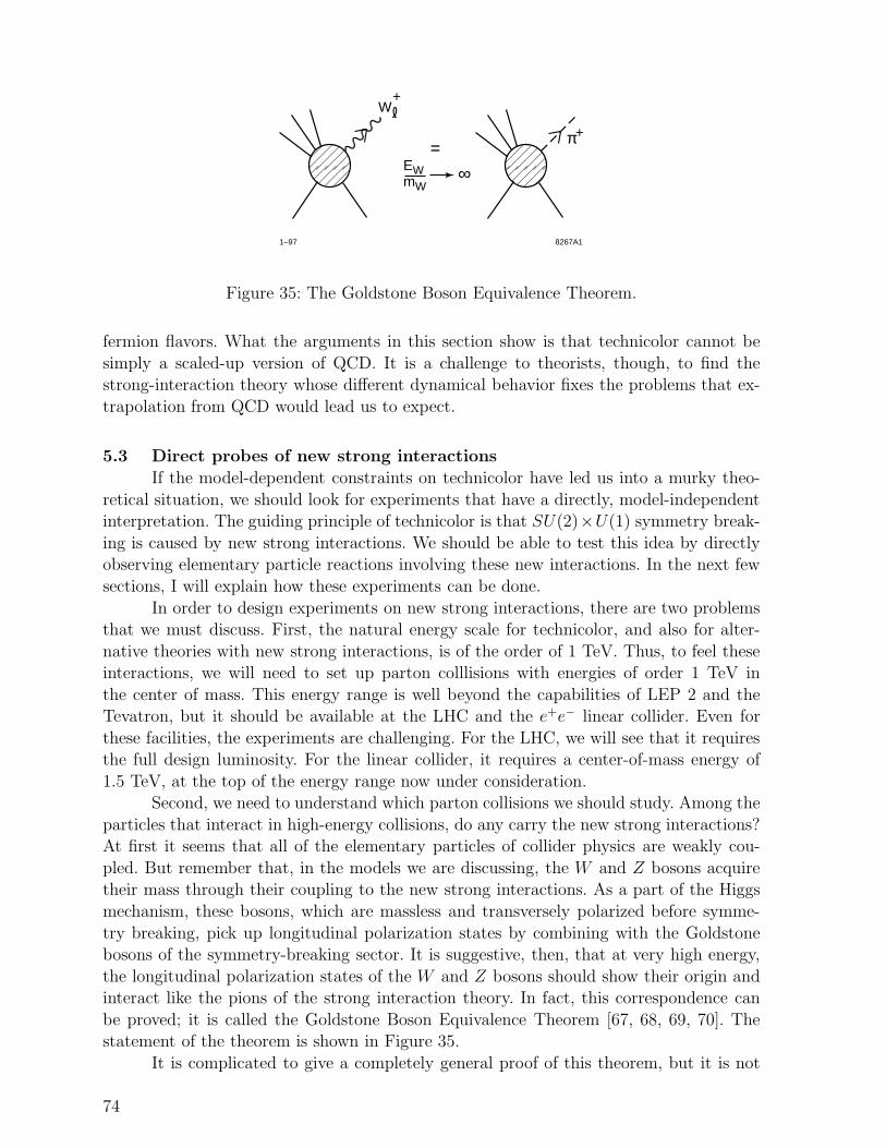
��yy ∞
1–97 8267A1
W
=EWmW
+ ��yyπ+
Figure 35: The Goldstone Boson Equivalence Theorem.
fermion flavors. What the arguments in this section show is that technicolor cannot be
simply a scaled-up version of QCD. It is a challenge to theorists, though, to find thestrong-interaction theory whose different dynamical behavior fixes the problems that ex-
trapolation from QCD would lead us to expect.
5.3 Direct probes of new strong interactions
If the model-dependent constraints on technicolor have led us into a murky theo-
retical situation, we should look for experiments that have a directly, model-independentinterpretation. The guiding principle of technicolor is that SU(2)×U(1) symmetry break-
ing is caused by new strong interactions. We should be able to test this idea by directlyobserving elementary particle reactions involving these new interactions. In the next few
sections, I will explain how these experiments can be done.
In order to design experiments on new strong interactions, there are two problemsthat we must discuss. First, the natural energy scale for technicolor, and also for alter-
native theories with new strong interactions, is of the order of 1 TeV. Thus, to feel theseinteractions, we will need to set up parton colllisions with energies of order 1 TeV in
the center of mass. This energy range is well beyond the capabilities of LEP 2 and theTevatron, but it should be available at the LHC and the e+e− linear collider. Even for
these facilities, the experiments are challenging. For the LHC, we will see that it requiresthe full design luminosity. For the linear collider, it requires a center-of-mass energy of
1.5 TeV, at the top of the energy range now under consideration.Second, we need to understand which parton collisions we should study. Among the
particles that interact in high-energy collisions, do any carry the new strong interactions?At first it seems that all of the elementary particles of collider physics are weakly cou-
pled. But remember that, in the models we are discussing, the W and Z bosons acquiretheir mass through their coupling to the new strong interactions. As a part of the Higgs
mechanism, these bosons, which are massless and transversely polarized before symme-
try breaking, pick up longitudinal polarization states by combining with the Goldstonebosons of the symmetry-breaking sector. It is suggestive, then, that at very high energy,
the longitudinal polarization states of the W and Z bosons should show their origin andinteract like the pions of the strong interaction theory. In fact, this correspondence can
be proved; it is called the Goldstone Boson Equivalence Theorem [67, 68, 69, 70]. Thestatement of the theorem is shown in Figure 35.
It is complicated to give a completely general proof of this theorem, but it is not
74
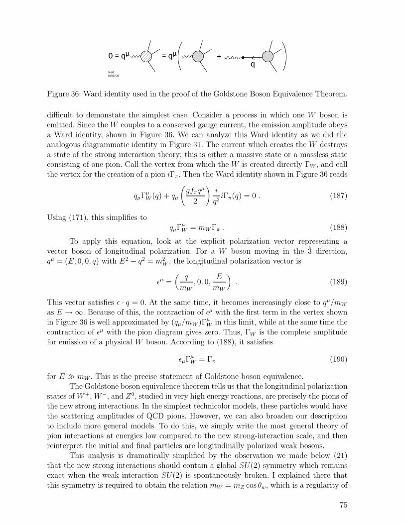
5–97 8303A25
0 = qµ = qµq�y +
Figure 36: Ward identity used in the proof of the Goldstone Boson Equivalence Theorem.
difficult to demonstate the simplest case. Consider a process in which one W boson isemitted. Since the W couples to a conserved gauge current, the emission amplitude obeys
a Ward identity, shown in Figure 36. We can analyze this Ward identity as we did theanalogous diagrammatic identity in Figure 31. The current which creates the W destroys
a state of the strong interaction theory; this is either a massive state or a massless stateconsisting of one pion. Call the vertex from which the W is created directly ΓW , and call
the vertex for the creation of a pion iΓπ. Then the Ward identity shown in Figure 36 reads
qµΓµW (q) + qµ
(gfπq
µ
2
)i
q2iΓπ(q) = 0 . (187)
Using (171), this simplifies to
qµΓµW = mWΓπ . (188)
To apply this equation, look at the explicit polarization vector representing a
vector boson of longitudinal polarization. For a W boson moving in the 3 direction,qµ = (E, 0, 0, q) with E2 − q2 = m2
W , the longitudinal polarization vector is
ǫµ =(
q
mW
, 0, 0,E
mW
). (189)
This vector satisfies ǫ · q = 0. At the same time, it becomes increasingly close to qµ/mW
as E → ∞. Because of this, the contraction of ǫµ with the first term in the vertex shown
in Figure 36 is well approximated by (qµ/mW )ΓµW in this limit, while at the same time the
contraction of ǫµ with the pion diagram gives zero. Thus, ΓW is the complete amplitudefor emission of a physical W boson. According to (188), it satisfies
ǫµΓµW = Γπ (190)
for E ≫ mW . This is the precise statement of Goldstone boson equivalence.The Goldstone boson equivalence theorem tells us that the longitudinal polarization
states of W+, W−, and Z0, studied in very high energy reactions, are precisely the pions ofthe new strong interactions. In the simplest technicolor models, these particles would have
the scattering amplitudes of QCD pions. However, we can also broaden our description
to include more general models. To do this, we simply write the most general theory ofpion interactions at energies low compared to the new strong-interaction scale, and then
reinterpret the initial and final particles are longitudinally polarized weak bosons.This analysis is dramatically simplified by the observation we made below (21)
that the new strong interactions should contain a global SU(2) symmetry which remainsexact when the weak interaction SU(2) is spontaneously broken. I explained there that
this symmetry is required to obtain the relation mW = mZ cos θw, which is a regularity of
75
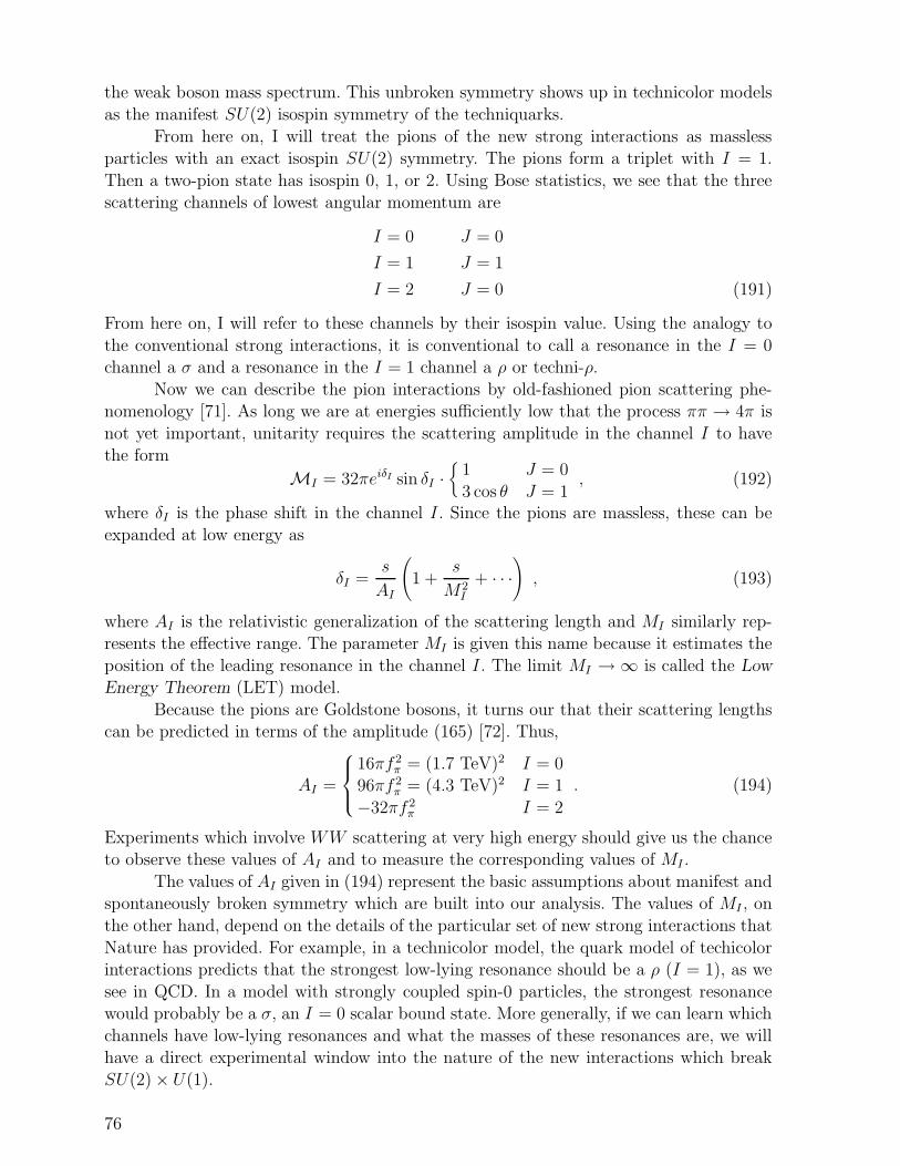
the weak boson mass spectrum. This unbroken symmetry shows up in technicolor models
as the manifest SU(2) isospin symmetry of the techniquarks.
From here on, I will treat the pions of the new strong interactions as masslessparticles with an exact isospin SU(2) symmetry. The pions form a triplet with I = 1.
Then a two-pion state has isospin 0, 1, or 2. Using Bose statistics, we see that the threescattering channels of lowest angular momentum are
I = 0 J = 0
I = 1 J = 1
I = 2 J = 0 (191)
From here on, I will refer to these channels by their isospin value. Using the analogy to
the conventional strong interactions, it is conventional to call a resonance in the I = 0channel a σ and a resonance in the I = 1 channel a ρ or techni-ρ.
Now we can describe the pion interactions by old-fashioned pion scattering phe-nomenology [71]. As long we are at energies sufficiently low that the process ππ → 4π is
not yet important, unitarity requires the scattering amplitude in the channel I to havethe form
MI = 32πeiδI sin δI ·{
1 J = 0
3 cos θ J = 1, (192)
where δI is the phase shift in the channel I. Since the pions are massless, these can beexpanded at low energy as
δI =s
AI
(1 +
s
M2I
+ · · ·), (193)
where AI is the relativistic generalization of the scattering length and MI similarly rep-resents the effective range. The parameter MI is given this name because it estimates the
position of the leading resonance in the channel I. The limit MI → ∞ is called the Low
Energy Theorem (LET) model.
Because the pions are Goldstone bosons, it turns our that their scattering lengthscan be predicted in terms of the amplitude (165) [72]. Thus,
AI =
16πf 2π = (1.7 TeV)2 I = 0
96πf 2π = (4.3 TeV)2 I = 1
−32πf 2π I = 2
. (194)
Experiments which involve WW scattering at very high energy should give us the chanceto observe these values of AI and to measure the corresponding values of MI .
The values of AI given in (194) represent the basic assumptions about manifest andspontaneously broken symmetry which are built into our analysis. The values of MI , on
the other hand, depend on the details of the particular set of new strong interactions that
Nature has provided. For example, in a technicolor model, the quark model of techicolorinteractions predicts that the strongest low-lying resonance should be a ρ (I = 1), as we
see in QCD. In a model with strongly coupled spin-0 particles, the strongest resonancewould probably be a σ, an I = 0 scalar bound state. More generally, if we can learn which
channels have low-lying resonances and what the masses of these resonances are, we willhave a direct experimental window into the nature of the new interactions which break
SU(2) × U(1).
76
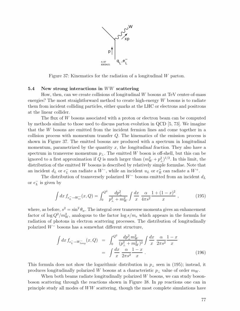
W
xp
p
4–97 8303A21
qL,e
L–
Figure 37: Kinematics for the radiation of a longitudinal W parton.
5.4 New strong interactions in WW scattering
How, then, can we create collisions of longitudinal W bosons at TeV center-of-mass
energies? The most straightforward method to create high-energy W bosons is to radiatethem from incident colliding particles, either quarks at the LHC or electrons and positrons
at the linear collider.The flux of W bosons associated with a proton or electron beam can be computed
by methods similar to those used to discuss parton evolution in QCD [5, 73]. We imagine
that the W bosons are emitted from the incident fermion lines and come together in acollision process with momentum transfer Q. The kinematics of the emission process is
shown in Figure 37. The emitted bosons are produced with a spectrum in longitudinalmomentum, parametrized by the quantity x, the longitudinal fraction. They also have a
spectrum in transverse momentum p⊥. The emitted W boson is off-shell, but this can beignored to a first approximation if Q is much larger than (m2
W + p2⊥)1/2. In this limit, the
distribution of the emitted W bosons is described by relatively simple formulae. Note thatan incident dL or e−L can radiate a W−, while an incident uL or e+R can radiate a W+.
The distribution of transversely polarized W− bosons emitted from an incident dLor e−L is given by
∫dx fe−
L→W−
tr(x,Q) =
∫ Q2
0
dp2⊥
p2⊥ +m2
W
∫dx
x
α
4πs2
1 + (1 − x)2
x, (195)
where, as before, s2 = sin2 θw. The integral over transverse momenta gives an enhancementfactor of logQ2/m2
W , analogous to the factor log s/me which appears in the formula for
radiation of photons in electron scattering processes. The distribution of longitudinallypolarized W− bosons has a somewhat different structure,
∫dx fe−
L→W−
long(x,Q) =
∫ Q2
0
dp2⊥m
2W
(p2⊥ +m2
W )2
∫dx
x
α
2πs2
1 − x
x
=∫dx
x
α
2πs2
1 − x
x. (196)
This formula does not show the logarithmic distribution in p⊥ seen in (195); instead, itproduces longitudinally polarized W bosons at a characteristic p⊥ value of order mW .
When both beams radiate longitudinally polarized W bosons, we can study boson-boson scattering through the reactions shown in Figure 38. In pp reactions one can in
principle study all modes of WW scattering, though the most complete simulations have
77
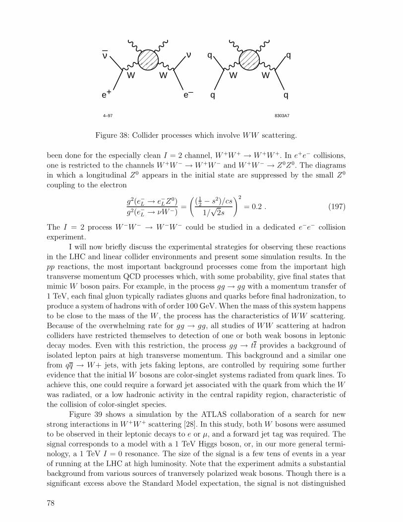
4–97 8303A7
W W W W
e+ e– q
q
q
qν_
�yy ��yyFigure 38: Collider processes which involve WW scattering.
been done for the especially clean I = 2 channel, W+W+ → W+W+. In e+e− collisions,
one is restricted to the channels W+W− →W+W− and W+W− → Z0Z0. The diagramsin which a longitudinal Z0 appears in the initial state are suppressed by the small Z0
coupling to the electron
g2(e−L → e−LZ0)
g2(e−L → νW−)=
((1
2− s2)/cs
1/√
2s
)2
= 0.2 . (197)
The I = 2 process W−W− → W−W− could be studied in a dedicated e−e− collisionexperiment.
I will now briefly discuss the experimental strategies for observing these reactionsin the LHC and linear collider environments and present some simulation results. In the
pp reactions, the most important background processes come from the important high
transverse momentum QCD processes which, with some probability, give final states thatmimic W boson pairs. For example, in the process gg → gg with a momentum transfer of
1 TeV, each final gluon typically radiates gluons and quarks before final hadronization, toproduce a system of hadrons with of order 100 GeV. When the mass of this system happens
to be close to the mass of the W , the process has the characteristics of WW scattering.Because of the overwhelming rate for gg → gg, all studies of WW scattering at hadron
colliders have restricted themselves to detection of one or both weak bosons in leptonicdecay modes. Even with this restriction, the process gg → tt provides a background of
isolated lepton pairs at high transverse momentum. This background and a similar onefrom qq → W+ jets, with jets faking leptons, are controlled by requiring some further
evidence that the initial W bosons are color-singlet systems radiated from quark lines. Toachieve this, one could require a forward jet associated with the quark from which the W
was radiated, or a low hadronic activity in the central rapidity region, characteristic ofthe collision of color-singlet species.
Figure 39 shows a simulation by the ATLAS collaboration of a search for new
strong interactions in W+W+ scattering [28]. In this study, both W bosons were assumedto be observed in their leptonic decays to e or µ, and a forward jet tag was required. The
signal corresponds to a model with a 1 TeV Higgs boson, or, in our more general termi-nology, a 1 TeV I = 0 resonance. The size of the signal is a few tens of events in a year
of running at the LHC at high luminosity. Note that the experiment admits a substantialbackground from various sources of tranversely polarized weak bosons. Though there is a
significant excess above the Standard Model expectation, the signal is not distinguished
78
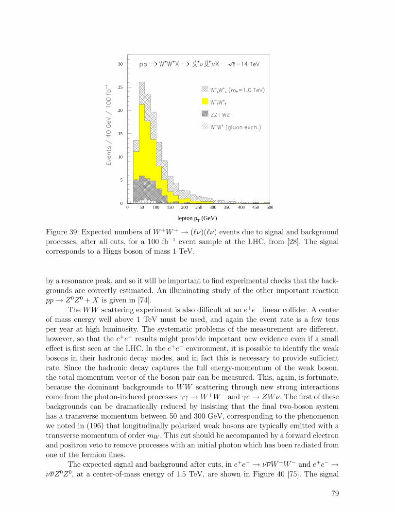
0
5
10
15
20
25
30
0 50 100 150 200 250 300 350 400 450 500
lepton pT (GeV)
Figure 39: Expected numbers of W+W+ → (ℓν)(ℓν) events due to signal and backgroundprocesses, after all cuts, for a 100 fb−1 event sample at the LHC, from [28]. The signal
corresponds to a Higgs boson of mass 1 TeV.
by a resonance peak, and so it will be important to find experimental checks that the back-
grounds are correctly estimated. An illuminating study of the other important reactionpp→ Z0Z0 +X is given in [74].
The WW scattering experiment is also difficult at an e+e− linear collider. A centerof mass energy well above 1 TeV must be used, and again the event rate is a few tens
per year at high luminosity. The systematic problems of the measurement are different,however, so that the e+e− results might provide important new evidence even if a small
effect is first seen at the LHC. In the e+e− environment, it is possible to identify the weakbosons in their hadronic decay modes, and in fact this is necessary to provide sufficient
rate. Since the hadronic decay captures the full energy-momentum of the weak boson,the total momentum vector of the boson pair can be measured. This, again, is fortunate,
because the dominant backgrounds to WW scattering through new strong interactionscome from the photon-induced processes γγ →W+W− and γe→ ZWν. The first of these
backgrounds can be dramatically reduced by insisting that the final two-boson system
has a transverse momentum between 50 and 300 GeV, corresponding to the phenomenonwe noted in (196) that longitudinally polarized weak bosons are typically emitted with a
transverse momentum of order mW . This cut should be accompanied by a forward electronand positron veto to remove processes with an initial photon which has been radiated from
one of the fermion lines.The expected signal and background after cuts, in e+e− → ννW+W− and e+e− →
ννZ0Z0, at a center-of-mass energy of 1.5 TeV, are shown in Figure 40 [75]. The signal
79
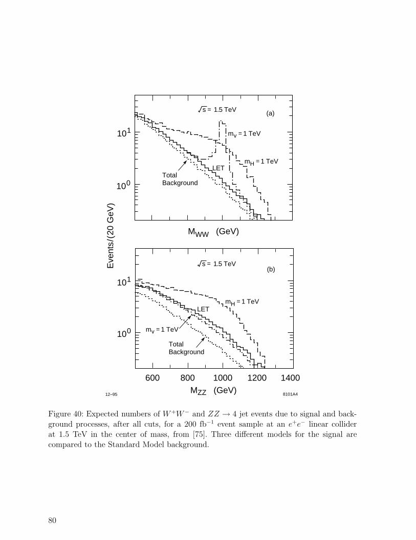
800 1000600 14001200
100
101
101
MZZ (GeV)
MWW (GeV)
Eve
nts/
(20
GeV
)
12–95 8101A4
mH = 1 TeV
mH = 1 TeV
mv = 1 TeV
mv = 1 TeV
(b)
LET
s = 1.5 TeV
100Total Background
(a)
LET
Total Background
s = 1.5 TeV
Figure 40: Expected numbers of W+W− and ZZ → 4 jet events due to signal and back-
ground processes, after all cuts, for a 200 fb−1 event sample at an e+e− linear colliderat 1.5 TeV in the center of mass, from [75]. Three different models for the signal are
compared to the Standard Model background.
80
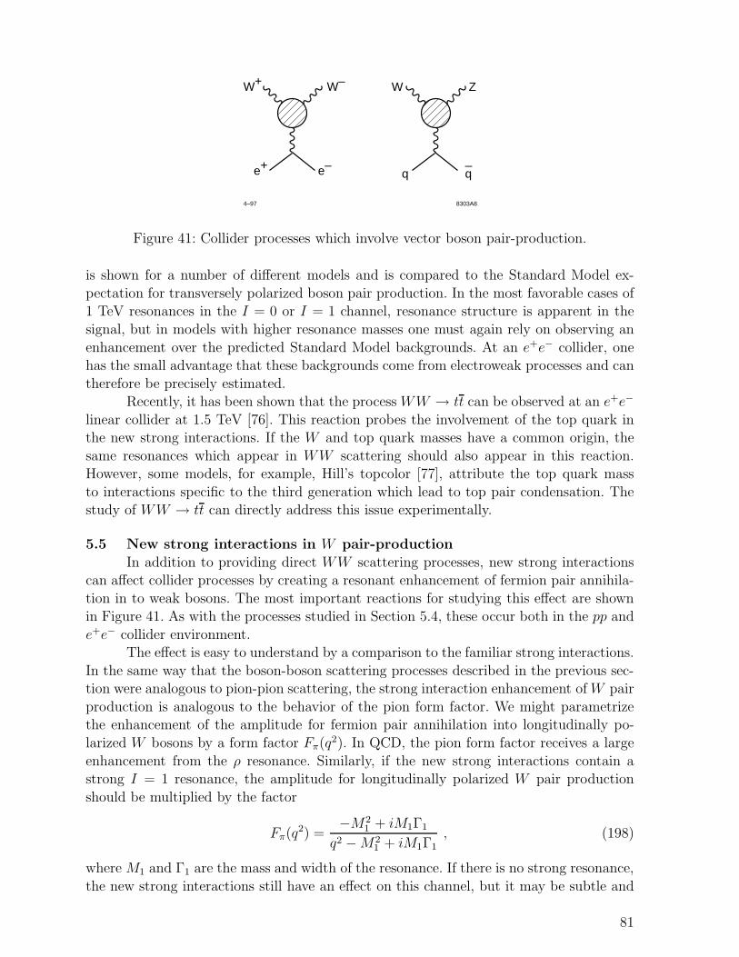
4–97 8303A8
Z
q_
q
WW+ W–
e+ e–�y �yFigure 41: Collider processes which involve vector boson pair-production.
is shown for a number of different models and is compared to the Standard Model ex-
pectation for transversely polarized boson pair production. In the most favorable cases of1 TeV resonances in the I = 0 or I = 1 channel, resonance structure is apparent in the
signal, but in models with higher resonance masses one must again rely on observing an
enhancement over the predicted Standard Model backgrounds. At an e+e− collider, onehas the small advantage that these backgrounds come from electroweak processes and can
therefore be precisely estimated.Recently, it has been shown that the process WW → tt can be observed at an e+e−
linear collider at 1.5 TeV [76]. This reaction probes the involvement of the top quark inthe new strong interactions. If the W and top quark masses have a common origin, the
same resonances which appear in WW scattering should also appear in this reaction.However, some models, for example, Hill’s topcolor [77], attribute the top quark mass
to interactions specific to the third generation which lead to top pair condensation. Thestudy of WW → tt can directly address this issue experimentally.
5.5 New strong interactions in W pair-production
In addition to providing direct WW scattering processes, new strong interactionscan affect collider processes by creating a resonant enhancement of fermion pair annihila-
tion in to weak bosons. The most important reactions for studying this effect are shownin Figure 41. As with the processes studied in Section 5.4, these occur both in the pp and
e+e− collider environment.The effect is easy to understand by a comparison to the familiar strong interactions.
In the same way that the boson-boson scattering processes described in the previous sec-tion were analogous to pion-pion scattering, the strong interaction enhancement of W pair
production is analogous to the behavior of the pion form factor. We might parametrizethe enhancement of the amplitude for fermion pair annihilation into longitudinally po-
larized W bosons by a form factor Fπ(q2). In QCD, the pion form factor receives a large
enhancement from the ρ resonance. Similarly, if the new strong interactions contain astrong I = 1 resonance, the amplitude for longitudinally polarized W pair production
should be multiplied by the factor
Fπ(q2) =
−M21 + iM1Γ1
q2 −M21 + iM1Γ1
, (198)
where M1 and Γ1 are the mass and width of the resonance. If there is no strong resonance,
the new strong interactions still have an effect on this channel, but it may be subtle and
81
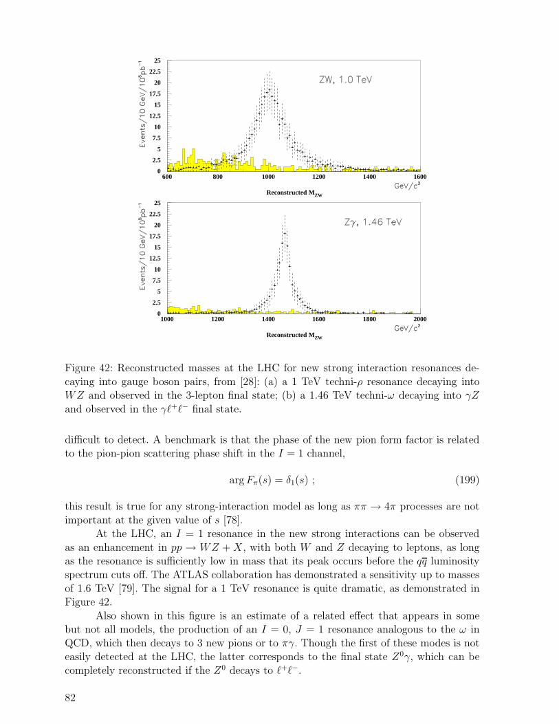
Reconstructed MZW
Reconstructed MZW
0
2.5
5
7.5
10
12.5
15
17.5
20
22.5
25
600 800 1000 1200 1400 1600
0
2.5
5
7.5
10
12.5
15
17.5
20
22.5
25
1000 1200 1400 1600 1800 2000
Figure 42: Reconstructed masses at the LHC for new strong interaction resonances de-
caying into gauge boson pairs, from [28]: (a) a 1 TeV techni-ρ resonance decaying intoWZ and observed in the 3-lepton final state; (b) a 1.46 TeV techni-ω decaying into γZ
and observed in the γℓ+ℓ− final state.
difficult to detect. A benchmark is that the phase of the new pion form factor is relatedto the pion-pion scattering phase shift in the I = 1 channel,
argFπ(s) = δ1(s) ; (199)
this result is true for any strong-interaction model as long as ππ → 4π processes are not
important at the given value of s [78].At the LHC, an I = 1 resonance in the new strong interactions can be observed
as an enhancement in pp → WZ + X, with both W and Z decaying to leptons, as longas the resonance is sufficiently low in mass that its peak occurs before the qq luminosity
spectrum cuts off. The ATLAS collaboration has demonstrated a sensitivity up to masses
of 1.6 TeV [79]. The signal for a 1 TeV resonance is quite dramatic, as demonstrated inFigure 42.
Also shown in this figure is an estimate of a related effect that appears in somebut not all models, the production of an I = 0, J = 1 resonance analogous to the ω in
QCD, which then decays to 3 new pions or to πγ. Though the first of these modes is noteasily detected at the LHC, the latter corresponds to the final state Z0γ, which can be
completely reconstructed if the Z0 decays to ℓ+ℓ−.
82
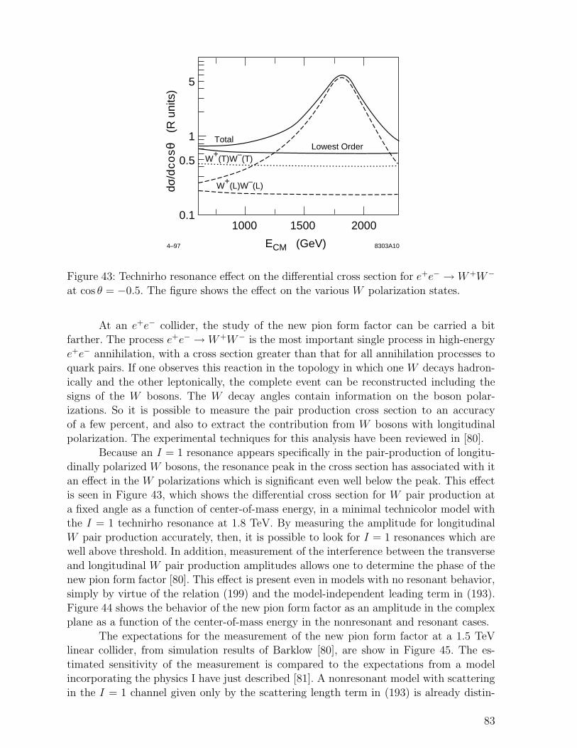
0.1
0.5
1
5
4–97 8303A10
Lowest OrderTotal
W+(L)W–(L)
W+(T)W–(T)
200015001000
ECM (GeV)
dσ/d
cosθ
(R
uni
ts)
Figure 43: Technirho resonance effect on the differential cross section for e+e− → W+W−
at cos θ = −0.5. The figure shows the effect on the various W polarization states.
At an e+e− collider, the study of the new pion form factor can be carried a bitfarther. The process e+e− → W+W− is the most important single process in high-energy
e+e− annihilation, with a cross section greater than that for all annihilation processes toquark pairs. If one observes this reaction in the topology in which one W decays hadron-
ically and the other leptonically, the complete event can be reconstructed including the
signs of the W bosons. The W decay angles contain information on the boson polar-izations. So it is possible to measure the pair production cross section to an accuracy
of a few percent, and also to extract the contribution from W bosons with longitudinalpolarization. The experimental techniques for this analysis have been reviewed in [80].
Because an I = 1 resonance appears specifically in the pair-production of longitu-dinally polarized W bosons, the resonance peak in the cross section has associated with it
an effect in the W polarizations which is significant even well below the peak. This effectis seen in Figure 43, which shows the differential cross section for W pair production at
a fixed angle as a function of center-of-mass energy, in a minimal technicolor model withthe I = 1 technirho resonance at 1.8 TeV. By measuring the amplitude for longitudinal
W pair production accurately, then, it is possible to look for I = 1 resonances which arewell above threshold. In addition, measurement of the interference between the transverse
and longitudinal W pair production amplitudes allows one to determine the phase of thenew pion form factor [80]. This effect is present even in models with no resonant behavior,
simply by virtue of the relation (199) and the model-independent leading term in (193).
Figure 44 shows the behavior of the new pion form factor as an amplitude in the complexplane as a function of the center-of-mass energy in the nonresonant and resonant cases.
The expectations for the measurement of the new pion form factor at a 1.5 TeVlinear collider, from simulation results of Barklow [80], are show in Figure 45. The es-
timated sensitivity of the measurement is compared to the expectations from a modelincorporating the physics I have just described [81]. A nonresonant model with scattering
in the I = 1 channel given only by the scattering length term in (193) is already distin-
83
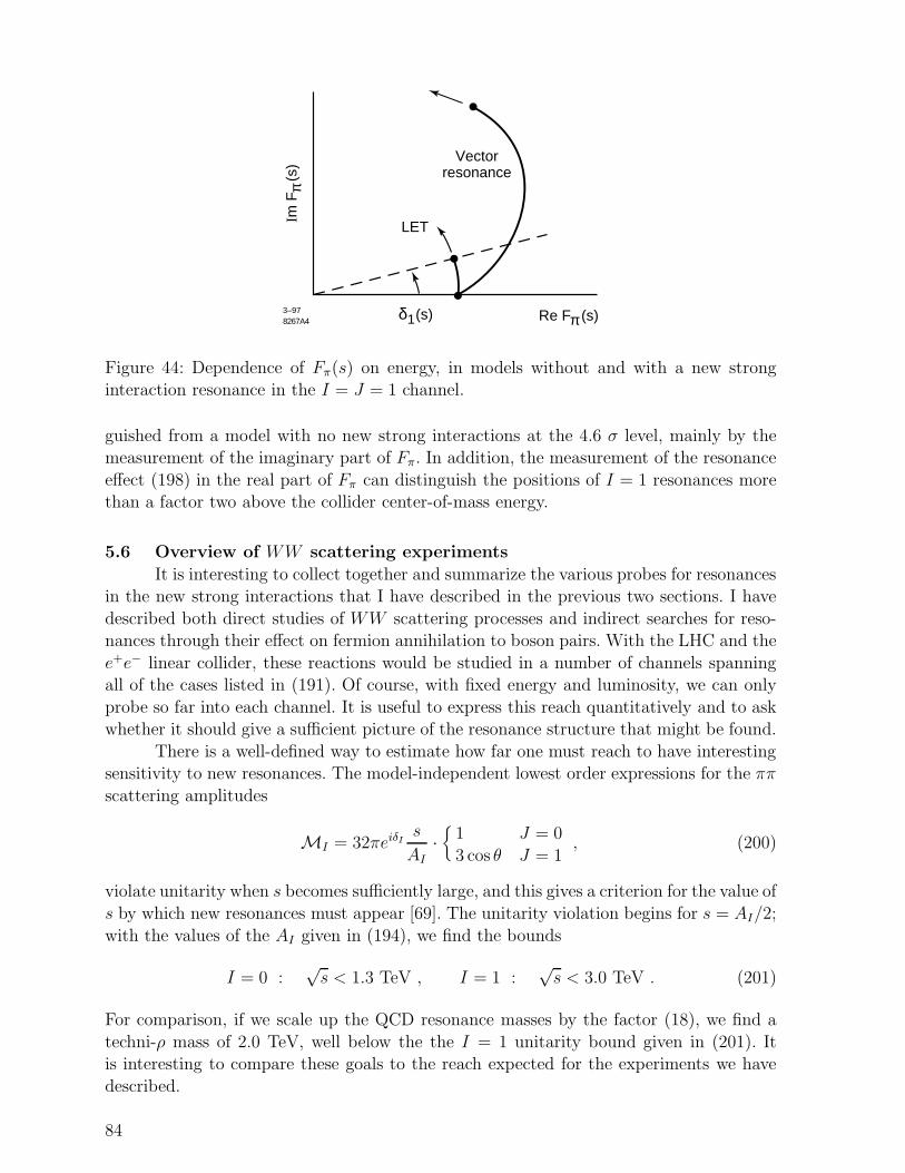
δ1(s)
Vector resonance
LET
Re Fπ (s)
Im F
π (s
)3–978267A4
Figure 44: Dependence of Fπ(s) on energy, in models without and with a new stronginteraction resonance in the I = J = 1 channel.
guished from a model with no new strong interactions at the 4.6 σ level, mainly by themeasurement of the imaginary part of Fπ. In addition, the measurement of the resonance
effect (198) in the real part of Fπ can distinguish the positions of I = 1 resonances morethan a factor two above the collider center-of-mass energy.
5.6 Overview of WW scattering experiments
It is interesting to collect together and summarize the various probes for resonancesin the new strong interactions that I have described in the previous two sections. I have
described both direct studies of WW scattering processes and indirect searches for reso-nances through their effect on fermion annihilation to boson pairs. With the LHC and the
e+e− linear collider, these reactions would be studied in a number of channels spanningall of the cases listed in (191). Of course, with fixed energy and luminosity, we can only
probe so far into each channel. It is useful to express this reach quantitatively and to askwhether it should give a sufficient picture of the resonance structure that might be found.
There is a well-defined way to estimate how far one must reach to have interestingsensitivity to new resonances. The model-independent lowest order expressions for the ππ
scattering amplitudes
MI = 32πeiδIs
AI·{
1 J = 0
3 cos θ J = 1, (200)
violate unitarity when s becomes sufficiently large, and this gives a criterion for the value of
s by which new resonances must appear [69]. The unitarity violation begins for s = AI/2;
with the values of the AI given in (194), we find the bounds
I = 0 :√s < 1.3 TeV , I = 1 :
√s < 3.0 TeV . (201)
For comparison, if we scale up the QCD resonance masses by the factor (18), we find a
techni-ρ mass of 2.0 TeV, well below the the I = 1 unitarity bound given in (201). Itis interesting to compare these goals to the reach expected for the experiments we have
described.
84
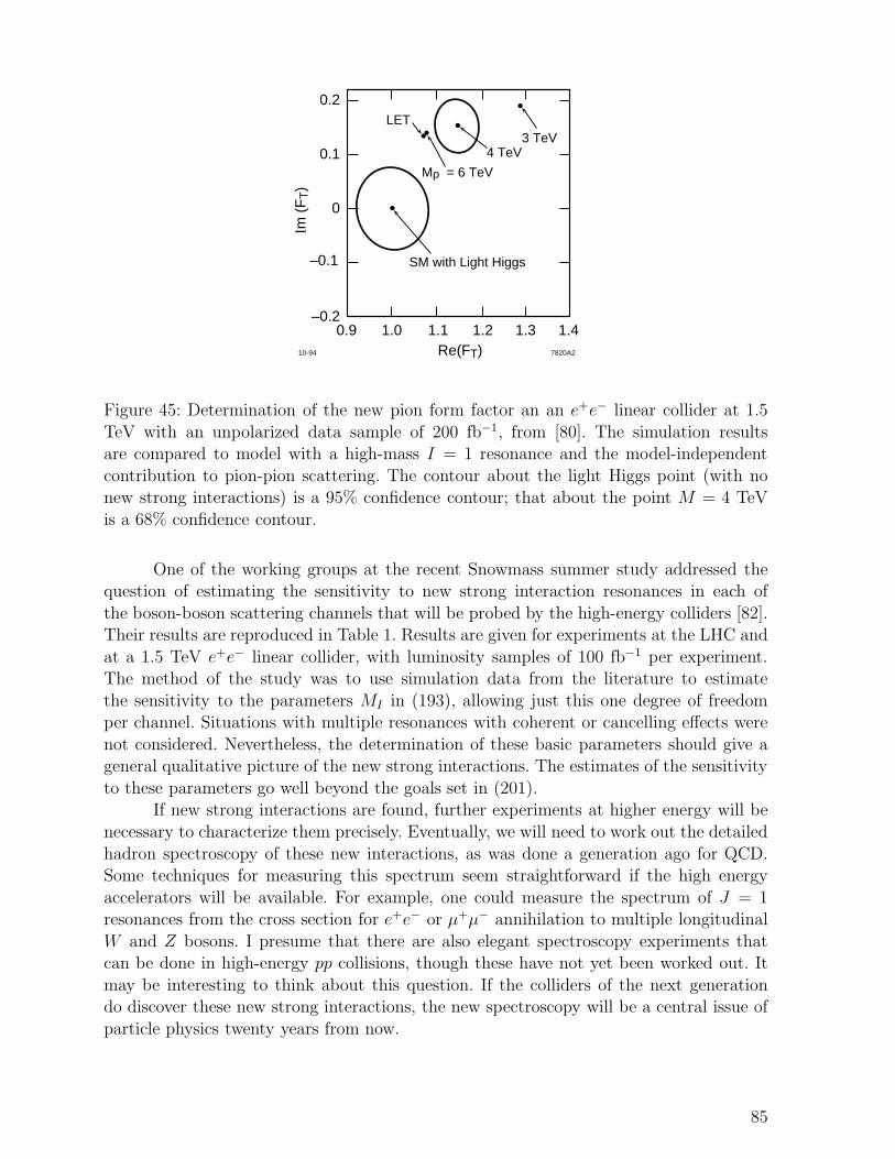
0.9–0.2
–0.1
0
0.1
0.2
1.1 1.2 1.3
SM with Light Higgs
Mρ = 6 TeV
4 TeV3 TeV
LET
1.41.0Re(FT) 7820A210-94
Im (
FT)
Figure 45: Determination of the new pion form factor an an e+e− linear collider at 1.5
TeV with an unpolarized data sample of 200 fb−1, from [80]. The simulation resultsare compared to model with a high-mass I = 1 resonance and the model-independent
contribution to pion-pion scattering. The contour about the light Higgs point (with nonew strong interactions) is a 95% confidence contour; that about the point M = 4 TeV
is a 68% confidence contour.
One of the working groups at the recent Snowmass summer study addressed thequestion of estimating the sensitivity to new strong interaction resonances in each of
the boson-boson scattering channels that will be probed by the high-energy colliders [82].Their results are reproduced in Table 1. Results are given for experiments at the LHC and
at a 1.5 TeV e+e− linear collider, with luminosity samples of 100 fb−1 per experiment.The method of the study was to use simulation data from the literature to estimate
the sensitivity to the parameters MI in (193), allowing just this one degree of freedomper channel. Situations with multiple resonances with coherent or cancelling effects were
not considered. Nevertheless, the determination of these basic parameters should give ageneral qualitative picture of the new strong interactions. The estimates of the sensitivity
to these parameters go well beyond the goals set in (201).If new strong interactions are found, further experiments at higher energy will be
necessary to characterize them precisely. Eventually, we will need to work out the detailed
hadron spectroscopy of these new interactions, as was done a generation ago for QCD.Some techniques for measuring this spectrum seem straightforward if the high energy
accelerators will be available. For example, one could measure the spectrum of J = 1resonances from the cross section for e+e− or µ+µ− annihilation to multiple longitudinal
W and Z bosons. I presume that there are also elegant spectroscopy experiments thatcan be done in high-energy pp collisions, though these have not yet been worked out. It
may be interesting to think about this question. If the colliders of the next generationdo discover these new strong interactions, the new spectroscopy will be a central issue of
particle physics twenty years from now.
85

Table 1: LHC and linear collider (‘NLC’) sensitivity to resonances in the new strong in-
teractions, from [82]. ‘Reach’ gives the value of the resonance mass corresponding to anenhancement of the cross section for boson-boson scattering at the 95% confidence level
obtained in Section VIB2. ‘Sample’ gives a representative set of errors for the determi-nation of a resonance mass from this enhancement. ‘Eff. L Reach’ gives the estimate of
the resonance mass for a 95% confidence level enhancement. All of these estimates are
based on simple parametrizations in which a single resonance dominates the scatteringcross section.
Machine Parton Level Process I Reach Sample Eff. L Reach
LHC qq′ → qq′ZZ 0 1600 1500+100−70 1500
LHC qq →WZ 1 1600 1550+50−50
LHC qq′ → qq′W+W+ 2 1950 2000+250−200
NLC e+e− → ννZZ 0 1800 1600+180−120 2000
NLC e+e− → ννtt 0 1600 1500+450−160
NLC e+e− → W+W− 1 4000 3000+180−150
5.7 Observable effects of extended technicolor
Beyond these general methods for observing new strong interactions, which apply
to any model in which electroweak symmetry breaking has a strong-coupling origin, eachspecific model leads to its own model-dependent predictions. Typically, these predictions
can be tested at energies below the TeV scale, so they provide phenomena that canbe explored before the colliders of the next generation reach their ultimate energy and
luminosity. On the other hand, these predictions are specific to their context. Excludingone such phenomenon rules out a particular model but not necessarily the whole class of
strong-coupled theories. We have seen an example of this already in Section 5.2, where thestrong constraints on technicolor models from precision electroweak physics force viable
models to have particular dynamical behavior but do not exclude these models completely.In this section, I would like to highlight three such predictions specifically associated
with technicolor theories. These three phenomena illustrate the range of possible effects
that might be found. A systematic survey of the model-dependent predictions of modelsof strongly-coupled electroweak symmetry breaking is given in [82].
All three of these predictions are associated with the extended technicolor mech-anism of quark and lepton mass generation described at the end of Section 5.1 and in
Figure 32. To see the first prediction, note from the figure that the Standard Model quan-tum numbers of the external fermion must be carried either by the techniquark or by
the ETC gauge boson. The simplest possibility is to assign the techniquarks the quan-
86
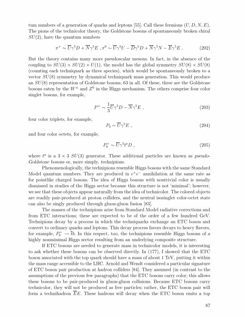
tum numbers of a generation of quarks and leptons [55]. Call these fermions (U,D,N,E).
The pions of the technicolor theory, the Goldstone bosons of spontaneously broken chiral
SU(2), have the quantum numbers
π+ ∼ Uγ5D +Nγ5E , π0 ∼ Uγ5U −Dγ5D +Nγ5N − Eγ5E . (202)
But the theory contains many more pseudoscalar mesons. In fact, in the absence of the
coupling to SU(3) × SU(2) × U(1), the model has the global symmetry SU(8) × SU(8)(counting each techniquark as three species), which would be spontaneously broken to a
vector SU(8) symmetry by dynamical techniquark mass generation. This would producean SU(8) representation of Goldstone bosons, 63 in all. Of these, three are the Goldstone
bosons eaten by the W± and Z0 in the Higgs mechanism. The others comprise four colorsinglet bosons, for example,
P+ ∼ 1
3Uγ5D −Nγ5E , (203)
four color triplets, for example,
P3 ∼ Uγ5E , (204)
and four color octets, for example,
P+8 ∼ Uγ5taD , (205)
where ta is a 3 × 3 SU(3) generator. These additional particles are known as pseudo-
Goldstone bosons or, more simply, technipions.
Phenomenologically, the technipions resemble Higgs bosons with the same StandardModel quantum numbers. They are produced in e+e− annihilation at the same rate as
for pointlike charged bosons. The idea of Higgs bosons with nontrivial color is usuallydismissed in studies of the Higgs sector because this structure is not ‘minimal’; however,
we see that these objects appear naturally from the idea of technicolor. The colored objectsare readily pair-produced at proton colliders, and the neutral isosinglet color-octet state
can also be singly produced through gluon-gluon fusion [83].The masses of the technipions arise from Standard Model radiative corrections and
from ETC interactions; these are expected to be of the order of a few hundred GeV.Technipions decay by a process in which the techniquarks exchange an ETC boson and
convert to ordinary quarks and leptons. This decay process favors decays to heavy flavors,for example, P+
8 → tb. In this respect, too, the technipions resemble Higgs bosons of a
highly nonminimal Higgs sector resulting from an underlying composite structure.If ETC bosons are needed to generate mass in technicolor models, it is interesting
to ask whether these bosons can be observed directly. In (177), I showed that the ETC
boson associated with the top quark should have a mass of about 1 TeV, putting it withinthe mass range accessible to the LHC. Arnold and Wendt considered a particular signature
of ETC boson pair production at hadron colliders [84]. They assumed (in contrast to theassumptions of the previous few paragraphs) that the ETC bosons carry color; this allows
these bosons to be pair-produced in gluon-gluon collisions. Because ETC bosons carrytechnicolor, they will not be produced as free particles; rather, the ETC boson pair will
form a technihadron EE. These hadrons will decay when the ETC boson emits a top
87
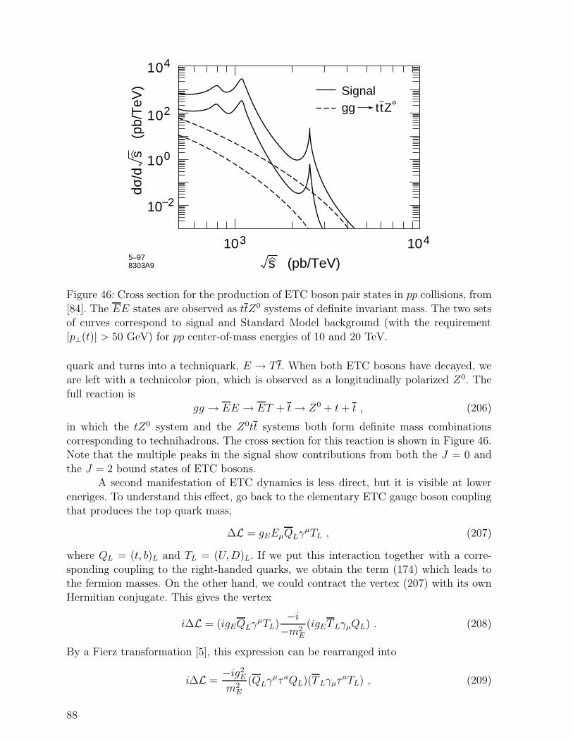
103 104
10–2
100
102
104
5–97 8303A9
Signal gg ttZ°
s (pb/TeV)
dσ/d
s
(pb
/TeV
)
Figure 46: Cross section for the production of ETC boson pair states in pp collisions, from
[84]. The EE states are observed as ttZ0 systems of definite invariant mass. The two setsof curves correspond to signal and Standard Model background (with the requirement
|p⊥(t)| > 50 GeV) for pp center-of-mass energies of 10 and 20 TeV.
quark and turns into a techniquark, E → Tt. When both ETC bosons have decayed, weare left with a technicolor pion, which is observed as a longitudinally polarized Z0. The
full reaction is
gg → EE → ET + t→ Z0 + t+ t , (206)
in which the tZ0 system and the Z0tt systems both form definite mass combinations
corresponding to technihadrons. The cross section for this reaction is shown in Figure 46.Note that the multiple peaks in the signal show contributions from both the J = 0 and
the J = 2 bound states of ETC bosons.A second manifestation of ETC dynamics is less direct, but it is visible at lower
eneriges. To understand this effect, go back to the elementary ETC gauge boson couplingthat produces the top quark mass,
∆L = gEEµQLγµTL , (207)
where QL = (t, b)L and TL = (U,D)L. If we put this interaction together with a corre-
sponding coupling to the right-handed quarks, we obtain the term (174) which leads tothe fermion masses. On the other hand, we could contract the vertex (207) with its own
Hermitian conjugate. This gives the vertex
i∆L = (igEQLγµTL)
−i−m2
E
(igETLγµQL) . (208)
By a Fierz transformation [5], this expression can be rearranged into
i∆L =−ig2
E
m2E
(QLγµτaQL)(TLγµτ
aTL) , (209)
88
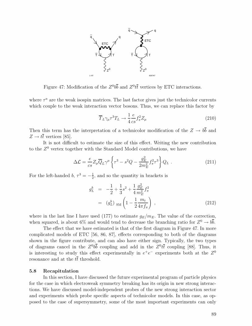
1–97 8267A7
Z0 Z0
q
ETCETC
q_
q_
q
T_
T_
T T
Figure 47: Modification of the Z0bb and Z0tt vertices by ETC interactions.
where τa are the weak isospin matrices. The last factor gives just the technicolor currents
which couple to the weak interaction vector bosons. Thus, we can replace this factor by
TLγµτ3TL → 1
4
e
csf 2πZµ (210)
Then this term has the interpretation of a technicolor modification of the Z → bb andZ → tt vertices [85].
It is not difficult to estimate the size of this effect. Writing the new contributionto the Z0 vertex together with the Standard Model contributions, we have
∆L =e
csZµQLγ
µ
{τ 3 − s2Q− g2
E
2m2E
f 2πτ
3
}QL . (211)
For the left-handed b, τ 3 = −12, and so the quantity in brackets is
gbL = −1
2+
1
3s2 +
1
4
g2E
m2E
f 2π
= (gbL) SM
(1 − 1
2
mt
4πfπ
), (212)
where in the last line I have used (177) to estimate gE/mE . The value of the correction,when squared, is about 6% and would tend to decrease the branching ratio for Z0 → bb.
The effect that we have estimated is that of the first diagram in Figure 47. In morecomplicated models of ETC [56, 86, 87], effects corresponding to both of the diagrams
shown in the figure contribute, and can also have either sign. Typically, the two types
of diagrams cancel in the Z0bb coupling and add in the Z0tt coupling [88]. Thus, itis interesting to study this effect experimentally in e+e− experiments both at the Z0
resonance and at the tt threshold.
5.8 Recapitulation
In this section, I have discussed the future experimental program of particle physicsfor the case in which electroweak symmetry breaking has its origin in new strong interac-
tions. We have discussed model-independent probes of the new strong interaction sectorand experiments which probe specific aspects of technicolor models. In this case, as op-
posed to the case of supersymmetry, some of the most important experiments can only
89
be done at very high energies and luminosities, corresponding to the highest values being
considered for the next generation of colliders. Nevertheless, I have argued that, if plans
now proposed can be realized, these experiments form a rich program which provides abroad experimental view of the new interactions.
Two sets of contrasting viewpoints appeared in our analysis. The first was the con-trast between experiments that test model-dependent as opposed to model-independent
conclusions. The search for technipions, for corrections to the Ztt vertex, and for otherspecific manifestations of technicolor theories can be carried out at energies well below
the 1 TeV scale. In fact, the precision electroweak experiments and the current precisiondetermination of the Z0 → bb branching ratio already strongly constrain technicolor the-
ories. However, such constraints can be evaded by clever model-building. If an anomalypredicted by technicolor is found, it will be important and remarkable. But in either case,
we will need to carry out the TeV-energy experiments to see the new interactions directlyand to clearly establish their properties.
The second set of contrasts, which we saw also in our study of supersymmetry,comes from the different viewpoints offered by pp and e+e− colliders. In the search for
anomalies, the use of both types of experiments clearly offers a broader field for discovery.
But these two types of facilities also bring different information to the more systematicprogram of study of the new strong interactions summarized in Table 1. The table makes
quantitative the powerful capabilities of the LHC to explore the new strong interactionsector. But it also shows that an e+e− linear collider adds to the LHC an exceptional
sensitivity in the I = 1 channel, reaching well past the unitarity bound, and sensitivity tothe process W+W− → tt, which tests the connection between the new strong interactions
and the top quark mass generation. Again in this example, we see how the LHC and thelinear collider, taken together, provide the information for a broad and coherent picture
of physics beyond the standard model.
6. Conclusions
This concludes our grand tour of theoretical ideas about what physics waits forus at this and the next generation of high-energy colliders. I have structured my pre-
sentation around two specific concrete models of new physics—supersymmetry and tech-nicolor. These models contrast greatly in their details and call for completely different
experimental programs. Nevertheless, they have some common features that I would liketo emphasize.
First of all, these models give examples of solutions to the problem I have argued isthe highest-priority problem in elementary particle physics, the mechanism of electroweak
symmetry breaking. Much work has been devoted to ‘minimal’ solutions to this problem,in which the future experimental program should be devoted to finding a few, or even just
one, Higgs scalar bosons. It is possible that Nature works in this way. But, for myself, I
do not believe it. Through these examples, I have tried to explain a very different viewof electroweak symmetry breaking, that this phenomenon arises from a new principle of
physics, and that its essential simplicity is found not by counting the number of particlesin the model but by understanding that the model is built around a coherent physical
mechanism. New principles have deep implications, and we have seen in our two examplesthat these can lead to a broad and fascinating experimental program.
If my viewpoint is right, these new phenomena are waiting for us, perhaps already
90
at the LEP 2 and Tevatron experiments of the next few years, and at the latest at the LHC
and the e+e− linear collider. If the new physical principle that we are seeking explains the
origin of Z and W masses, it cannot be too far away. In each of the models that I havediscussed, I have given a quantitative estimate of the energy reach required. At the next
generation of colliders, we will be there.For those of you who are now students of elementary particle physics, this conclu-
sion comes with both discouraging and encouraging messages. The discouragement comesfrom the long time scale required to construct new accelerator facilities and to carry out
the large-scale experiments that are now required on the frontier. Some of your teacherscan remember a time when a high-energy physics experiment could be done in one year.
Today, the time scale is of order ten years, or longer if the whole process of designing andconstructing the accelerator is considered.
The experiments that I have described put a premium not only on high energybut also high luminosity. This means that not only the experiments but also the accel-
erator designs required for these studies will require careful thinking and brilliant newideas. During the school, Alain Blondel was fond of repeating, ‘Inverse picobarns must be
earned!’ The price of inverse femtobarns is even higher. Thus, I strongly encourage you to
become involved in the problems of accelerator design and the interaction of acceleratorswith experiments, to search for solutions to the challenging problems that must be solve
to carry out experiments at 1 TeV and above.The other side of the message is filled with promise. If we can have the patience
to wait over the long time intervals that our experiments require, and to solve the tech-nical problems that they pose, we will eventually arrive at the physics responsible for
electroweak symmetry breaking. If the conception that I have argued for in these lec-tures is correct, this will be genuinely a new fundamental scale in physics, with new
interactions and a rich phenomenological structure. Though the experimental discoveryand clarification of this structure will be complex, the accelerators planned for the next
generation—the LHC and the e+e− linear collider—will provide the powerful tools andanalysis methods that we will require. This is the next frontier in elementary particle
physics, and it is waiting for you. Enjoy it when it arrives!
Acknowledgments
I am grateful to Belen Gavela, Matthias Neubert, and Nick Ellis for inviting me
to speak at the European School, to Alain Blondel, Susannah Tracy, and Egil Lillestolfor providing the very pleasant arrangements for the school, to the students at the school
for their enthusiasm and for their criticisms, and to Erez Etzion, Morris Swartz, and IanHinchliffe for comments on the manuscript. This work was supported by the Department
of Energy under contract DE–AC03–76SF00515.
91
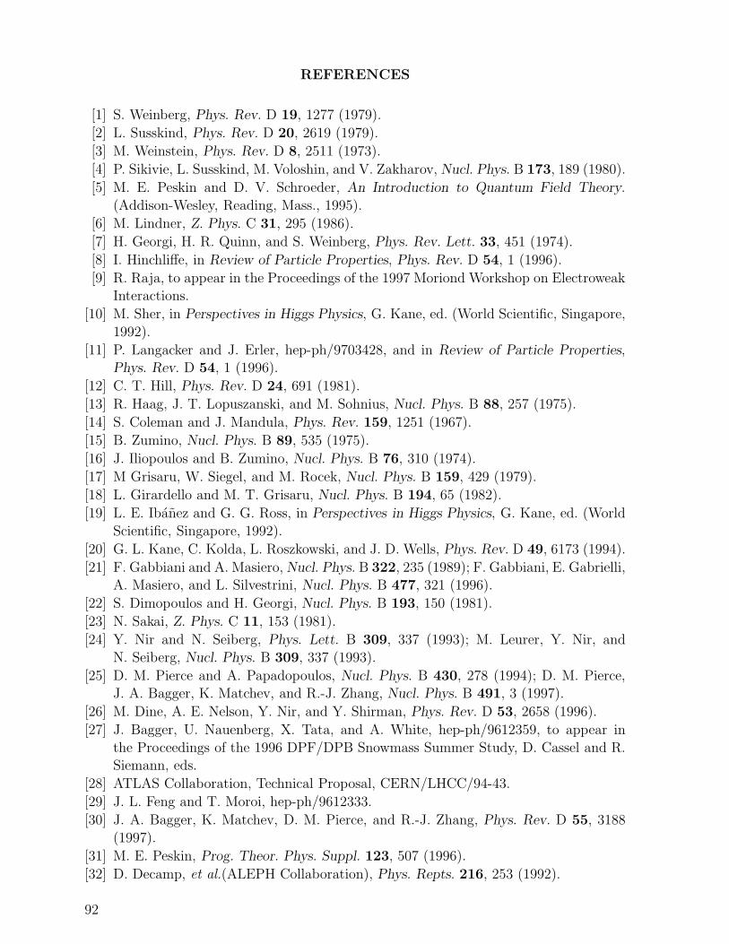
REFERENCES
[1] S. Weinberg, Phys. Rev. D 19, 1277 (1979).
[2] L. Susskind, Phys. Rev. D 20, 2619 (1979).
[3] M. Weinstein, Phys. Rev. D 8, 2511 (1973).
[4] P. Sikivie, L. Susskind, M. Voloshin, and V. Zakharov, Nucl. Phys. B 173, 189 (1980).
[5] M. E. Peskin and D. V. Schroeder, An Introduction to Quantum Field Theory.
(Addison-Wesley, Reading, Mass., 1995).
[6] M. Lindner, Z. Phys. C 31, 295 (1986).
[7] H. Georgi, H. R. Quinn, and S. Weinberg, Phys. Rev. Lett. 33, 451 (1974).
[8] I. Hinchliffe, in Review of Particle Properties, Phys. Rev. D 54, 1 (1996).
[9] R. Raja, to appear in the Proceedings of the 1997 Moriond Workshop on ElectroweakInteractions.
[10] M. Sher, in Perspectives in Higgs Physics, G. Kane, ed. (World Scientific, Singapore,
1992).
[11] P. Langacker and J. Erler, hep-ph/9703428, and in Review of Particle Properties,Phys. Rev. D 54, 1 (1996).
[12] C. T. Hill, Phys. Rev. D 24, 691 (1981).
[13] R. Haag, J. T. Lopuszanski, and M. Sohnius, Nucl. Phys. B 88, 257 (1975).
[14] S. Coleman and J. Mandula, Phys. Rev. 159, 1251 (1967).
[15] B. Zumino, Nucl. Phys. B 89, 535 (1975).
[16] J. Iliopoulos and B. Zumino, Nucl. Phys. B 76, 310 (1974).
[17] M Grisaru, W. Siegel, and M. Rocek, Nucl. Phys. B 159, 429 (1979).
[18] L. Girardello and M. T. Grisaru, Nucl. Phys. B 194, 65 (1982).
[19] L. E. Ibanez and G. G. Ross, in Perspectives in Higgs Physics, G. Kane, ed. (World
Scientific, Singapore, 1992).
[20] G. L. Kane, C. Kolda, L. Roszkowski, and J. D. Wells, Phys. Rev. D 49, 6173 (1994).
[21] F. Gabbiani and A. Masiero, Nucl. Phys. B 322, 235 (1989); F. Gabbiani, E. Gabrielli,A. Masiero, and L. Silvestrini, Nucl. Phys. B 477, 321 (1996).
[22] S. Dimopoulos and H. Georgi, Nucl. Phys. B 193, 150 (1981).
[23] N. Sakai, Z. Phys. C 11, 153 (1981).
[24] Y. Nir and N. Seiberg, Phys. Lett. B 309, 337 (1993); M. Leurer, Y. Nir, and
N. Seiberg, Nucl. Phys. B 309, 337 (1993).
[25] D. M. Pierce and A. Papadopoulos, Nucl. Phys. B 430, 278 (1994); D. M. Pierce,J. A. Bagger, K. Matchev, and R.-J. Zhang, Nucl. Phys. B 491, 3 (1997).
[26] M. Dine, A. E. Nelson, Y. Nir, and Y. Shirman, Phys. Rev. D 53, 2658 (1996).
[27] J. Bagger, U. Nauenberg, X. Tata, and A. White, hep-ph/9612359, to appear in
the Proceedings of the 1996 DPF/DPB Snowmass Summer Study, D. Cassel and R.Siemann, eds.
[28] ATLAS Collaboration, Technical Proposal, CERN/LHCC/94-43.
[29] J. L. Feng and T. Moroi, hep-ph/9612333.
[30] J. A. Bagger, K. Matchev, D. M. Pierce, and R.-J. Zhang, Phys. Rev. D 55, 3188
(1997).
[31] M. E. Peskin, Prog. Theor. Phys. Suppl. 123, 507 (1996).
[32] D. Decamp, et al.(ALEPH Collaboration), Phys. Repts. 216, 253 (1992).
92

[33] H. Baer, V. Barger, D. Karatas, and X. Tata, Phys. Rev. D 36, 96 (1987); H. Baer,
X. Tata, and J. Woodside, Phys. Rev. D 42, 1568 (1990).
[34] R. M. Barnett, J. F. Gunion, and H. E. Haber, Phys. Rev. D 37, 1892 (1988).
[35] H. Baer, X. Tata, and J. Woodside, Phys. Rev. D 45, 142 (1992).
[36] S. Dimopoulos, M. Dine, S. Raby, and S. Thomas, Phys. Rev. Lett. 76, 3494 (1996).
[37] J. Ellis, K. Enqvist, D. Nanopoulos, and F. Zwirner, Mod. Phys. Lett A 1, 57 (1986).
[38] R. Barbieri and G. Giudice, Nucl. Phys. B 306, 63 (1988).
[39] G. Anderson and D. Castano, Phys. Rev. D 52, 1693 (1995).
[40] G. F. Giudice, et al., hep-ph/9602207.
[41] D. Amidei and R. Brock, eds., Future Electroweak Physics at the Fermilab Tevatron.FERMILAB-Pub-96/082.
[42] I. Hinchliffe, F. E. Paige, M. D. Shapiro, J. Soderqvist, and W. Yao, Phys. Rev. D
55, 5520 (1997).
[43] G. Loew, et al., International Linear Collider Technical Review Committee Report
1995. SLAC-Report-471 (1995).
[44] S. Kuhlman, et al., Physics and Technology of the Next Linear Collider. BNL 52-
502, Fermilab-PUB-96/112, LBNL-PUB-5425, SLAC report 485, UCRL-ID-124160(1996).
[45] T. Tsukamoto, K. Fujii, H. Murayama, M. Yamaguchi, and Y. Okada, Phys. Rev. D
51, 3153 (1995).
[46] M. M. Nojiri, K. Fujii, and T. Tsukamoto, Phys. Rev. D 54, 6756 (1996).
[47] M. N. Danielson, et al., to appear in the Proceedings of the 1996 DPF/DPB Snow-
mass Summer Study, D. Cassel and R. Siemann, eds.
[48] J. L. Feng, M. E. Peskin, H. Murayama, and X. Tata, Phys. Rev. D 52, 1418 (1995).
[49] J. L. Feng and D. E. Finnell, Phys. Rev. D 49, 2369 (1994).
[50] LHC Study Group, The Large Hadron Collider: Conceptual Design. CERN/AC/95-05 (LHC) (1995).
[51] S. Basa, Marseille Ph. D. thesis, 1994.
[52] H. Baer, C.-H. Chen, F. Paige, and X. Tata, Phys. Rev. D 50, 4508 (1994).
[53] S. Dimopoulos and L. Susskind, Nucl. Phys. B 155, 237 (1979).
[54] E. Eichten and K. Lane, Phys. Lett. B 90, 125 (1980).
[55] E. Farhi and L. Susskind, Phys. Rev. D 20, 3404 (1979).
[56] R. S. Chivukula, E. Gates, E. H. Simmons and J. Terning, Phys. Lett. B 311, 157
(1993); R. S. Chivukula, E. H. Simmons and J. Terning, Phys. Lett. B 331, 383(1994).
[57] S. Glashow, J. Iliopoulos, and L. Maiani, Phys. Rev. D 2, 1285 (1970).
[58] E. Eichten, K. Lane, and J. Preskill, Phys. Rev. Lett. 45, 225 (1980).
[59] S. Dimopoulos and J. Ellis, Nucl. Phys. B 182, 505 (1982).
[60] S. Dimopoulos, H. Georgi, and S. Raby, Phys. Lett. B 127, 101 (1983).
[61] L. Randall, Nucl. Phys. B 403, 122 (1993).
[62] H. Georgi, Nucl. Phys. B 416, 699 (1994).
[63] S. Raby, Nucl. Phys. B 187, 446 (1981).
[64] M. E. Peskin and T. Takeuchi, Phys. Rev. Lett. 65, 964 (1990), Phys. Rev. D 46,
381 (1992).
[65] B. Holdom, Phys. Rev. D 24, 1441 (1981).
93
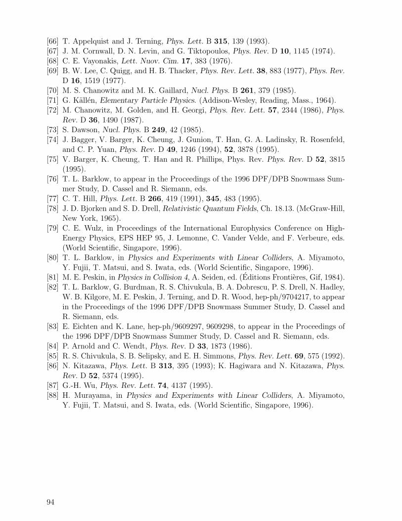
[66] T. Appelquist and J. Terning, Phys. Lett. B 315, 139 (1993).
[67] J. M. Cornwall, D. N. Levin, and G. Tiktopoulos, Phys. Rev. D 10, 1145 (1974).
[68] C. E. Vayonakis, Lett. Nuov. Cim. 17, 383 (1976).[69] B. W. Lee, C. Quigg, and H. B. Thacker, Phys. Rev. Lett. 38, 883 (1977), Phys. Rev.
D 16, 1519 (1977).[70] M. S. Chanowitz and M. K. Gaillard, Nucl. Phys. B 261, 379 (1985).
[71] G. Kallen, Elementary Particle Physics. (Addison-Wesley, Reading, Mass., 1964).[72] M. Chanowitz, M. Golden, and H. Georgi, Phys. Rev. Lett. 57, 2344 (1986), Phys.
Rev. D 36, 1490 (1987).[73] S. Dawson, Nucl. Phys. B 249, 42 (1985).
[74] J. Bagger, V. Barger, K. Cheung, J. Gunion, T. Han, G. A. Ladinsky, R. Rosenfeld,and C. P. Yuan, Phys. Rev. D 49, 1246 (1994), 52, 3878 (1995).
[75] V. Barger, K. Cheung, T. Han and R. Phillips, Phys. Rev. Phys. Rev. D 52, 3815(1995).
[76] T. L. Barklow, to appear in the Proceedings of the 1996 DPF/DPB Snowmass Sum-mer Study, D. Cassel and R. Siemann, eds.
[77] C. T. Hill, Phys. Lett. B 266, 419 (1991), 345, 483 (1995).
[78] J. D. Bjorken and S. D. Drell, Relativistic Quantum Fields, Ch. 18.13. (McGraw-Hill,New York, 1965).
[79] C. E. Wulz, in Proceedings of the International Europhysics Conference on High-Energy Physics, EPS HEP 95, J. Lemonne, C. Vander Velde, and F. Verbeure, eds.
(World Scientific, Singapore, 1996).[80] T. L. Barklow, in Physics and Experiments with Linear Colliders, A. Miyamoto,
Y. Fujii, T. Matsui, and S. Iwata, eds. (World Scientific, Singapore, 1996).[81] M. E. Peskin, in Physics in Collision 4, A. Seiden, ed. (Editions Frontieres, Gif, 1984).
[82] T. L. Barklow, G. Burdman, R. S. Chivukula, B. A. Dobrescu, P. S. Drell, N. Hadley,W. B. Kilgore, M. E. Peskin, J. Terning, and D. R. Wood, hep-ph/9704217, to appear
in the Proceedings of the 1996 DPF/DPB Snowmass Summer Study, D. Cassel andR. Siemann, eds.
[83] E. Eichten and K. Lane, hep-ph/9609297, 9609298, to appear in the Proceedings ofthe 1996 DPF/DPB Snowmass Summer Study, D. Cassel and R. Siemann, eds.
[84] P. Arnold and C. Wendt, Phys. Rev. D 33, 1873 (1986).
[85] R. S. Chivukula, S. B. Selipsky, and E. H. Simmons, Phys. Rev. Lett. 69, 575 (1992).[86] N. Kitazawa, Phys. Lett. B 313, 395 (1993); K. Hagiwara and N. Kitazawa, Phys.
Rev. D 52, 5374 (1995).[87] G.-H. Wu, Phys. Rev. Lett. 74, 4137 (1995).
[88] H. Murayama, in Physics and Experiments with Linear Colliders, A. Miyamoto,Y. Fujii, T. Matsui, and S. Iwata, eds. (World Scientific, Singapore, 1996).
94