arX

iv:h

ep-p

h/96

0831

9v2

21

Jan

1997

OUTP-96-11P (rev)

Evading the Cosmological Domain Wall Problem

Sebastian E. Larsson, Subir Sarkar and Peter L. White

Theoretical Physics, University of Oxford,

1 Keble Road, Oxford OX1 3NP

Abstract

Discrete symmetries are commonplace in field theoretical models but pose a

severe problem for cosmology since they lead to the formation of domain walls

during spontaneous symmetry breaking in the early universe. However if one

of the vacuua is favoured over the others, either energetically, or because of

initial conditions, it will eventually come to dominate the universe. Using

numerical methods, we study the evolution of the domain wall network for a

variety of field configurations in two and three dimensions and quantify the

rate at which the walls disappear. Good agreement is found with a recent

analytic estimate of the termination of the scaling regime of the wall network.

We conclude that there is no domain wall problem in the post-inflationary

universe for a weakly coupled field which is not in thermal equilibrium.

11.27.+d, 98.80.Cq

Typeset using REVTEX

[hep-ph/9608319]

1

I. INTRODUCTION

It was first noted by Zel’dovich, Kobzarev and Okun [1] that the restoration of sponta-neously broken discrete symmetries at high temperatures in the early universe poses severeproblems for its subsequent evolution.1 If the manifold M of degenerate vacua of the theoryis disconnected such that the homotopy group π0(M) is non-trivial, then sheet-like topolog-ical defects — domain walls — form at the boundaries of the different degenerate vacuuaduring the symmetry breaking phase transition, due to the existence of a causal particlehorizon in a decelerating universe [5]. The subsequent evolution of the wall network can bestudied using the techniques of percolation theory [6] and is such that the energy densityin the walls eventually comes to dominate the total energy density. The consequence is aninflationary phase which suffers from a ‘graceful exit’ problem in that it creates an universedevoid of any matter [7,8]. This can be avoided if the energy scale associated with thediscrete symmetry breaking is low enough; however in order to avoid generating excessiveanisotropy in the cosmic microwave background, the energy scale is further restricted to besmaller than ∼ 1 MeV [8]. Thus walls formed at any higher energy scale must be unstable

and have decayed away long before the present epoch.Attempts to introduce instability in domain walls which are expected in field theoretical

models have usually focussed on the role of non-renormalizable operators in the Lagrangianwhich may arise due to violation of global symmetries by Planck-scale gravitational effects[9]. These can ‘tilt’ the potential so as to favour one particular minimum which comes todominate the universe because the pressure of the favoured vacuum eventually wins out overthe restraining tension of the domain walls [1,10]. An example from particle physics is theaddition of a dimension-5 operator to the Lagrangian of the next-to-minimal supersymmet-ric standard model, in which the usual supersymmetric Higgs sector is supplemented bya gauge singlet superfield. Here Z3 domain walls are expected to be created in the Higgsfields during the electroweak symmetry breaking phase transition at T∼mW [11]. Howeverthe dissipation of the wall network in this case releases the contained energy as high energyinteracting particles which can interefere adversely with cosmological processes such as pri-mordial nucleosynthesis [12], hence the walls must disappear well before this epoch [13]. Inorder to quantify this constraint, it is neccessary to study the rate at which the wall networkdissipates for a given pressure difference between the different vacuua.

Another way in which the domain wall network may be destabilized is through a suitablechoice of initial conditions, viz. if the probability distribution has a bias for one vacuumover the others. This can be due to a prior non-equilibrium phase transition, for examplecosmological inflation, which can displace weakly coupled light fields from the minima oftheir potential [14], leading to a biased initial state [15]. It has been suggested that theresulting unstable domain walls in a light scalar field may be relevant for the formation oflarge-scale structure in the universe [16]. Recently, both an analytic [17] and a numerical[18] study of such biased domain walls have been carried out.

1It has been argued recently [2], following earlier work [3], that symmetry restoration may not

neccessarily occur, particularly if the scalar field has no gauge interactions. Whether this is still

true when non-perturbative effects are taken into account is currently under investigation [4].

2

In this paper we make a systematic investigation of domain wall network evolution forboth cases, viz. ‘pressure’ (§III (A)) and ‘bias’ (§III (B)) and and compare our resultswith simple analytic estimates of the rate at which the walls disappear, as well as withprevious numerical work [17,18]. We also study (§III (C)) the effects of biased initial fieldconfigurations resulting from a period of primordial inflation. We conclude (§IV) with adiscussion of the physical implications of our results.

II. NUMERICAL TECHNIQUES

The generic potential which exhibits the problem under discussion is

V (φ) = V0

(

φ2

φ20

− 1

)2

. (1)

This has two degenerate vacuua, φ = ±φ0 separated by a potential barrier V0, so that thespontaneous breaking of the Z2 symmetry when the universe cools below the temperatureT ∼ V0 will result in the formation of domain walls. We wish to simulate the evolution ofthe resulting wall network by solving the field equations on a specified lattice. The basicproblem in such numerical studies is that there are two very different length scales involved,viz. the wall width,

w0 ∼φ0√V0

, (2)

and the size of the simulation box. The first is constant in physical coordinates whilst thesecond must be large relative to a typical domain size, which scales with the expansion of theUniverse. However the wall thickness is in general much smaller than the size of of the wallnetwork so one can sensibly assume that the walls behave like two-dimensional relativisticmembranes, given that their internal structure is expected to be of negligible importancefor the evolution. Two routes have so far been pursued in applying this idea to computersimulations of domain wall dynamics.

Kawano [19] considered an effective action obtained by expanding in w0/R, where R isthe radius of curvature of the wall, and retaining only the zeroth order term. The resultantNambu-type action yields [20] the evolution equation

R + 3a

aR(1 − R2) = −2(1 − R2)

R, (3)

where a is the cosmological scale-factor of the Robertson-Walker metric for an Einstein-DeSitter universe, gµν = diag[−1, a(t)2, a(t)2, a(t)2]. Unfortunately this otherwise attractiveapproach leads to severe numerical instabilities (of the type discussed in a slightly differentcontext [21]), hence cannot be fruitfully pursued.

The second approach, which we use in the present work is due to Press, Ryden andSpergel [22,23]. Consider the classical equation of motion for the Higgs field in an expandingbackground:

∂2φ

∂η2+ 2

d ln a

d ln η

1

η

∂φ

∂η−∇2φ = −a2 ∂V

∂φ, (4)

3

where η is the conformal time (dη ≡ dt/a(t)) which measures the comoving distance traversedby light since the big bang. Here the numerical problem is manifest in the a2 term on the rhswhich makes the potential barrier appear higher as time goes on, resulting in a wall solutionwhich grows increasingly narrow (in comoving cordinates) with time. In attempting toevolve an equation of this type directly one would find that the wall solutions in the φ fieldquickly become so narrow as to be unresolvable. The solution is to generalize the equationof motion to:

∂2φ

∂η2+ α

d ln a

d ln η

1

η

∂φ

∂η−∇2φ = −aβ ∂V

∂φ, (5)

and then set β = 0 in order to freeze the wall size in comoving coordinates. We also setα = 3 to ensure momentum conservation since this requires that we have [22]

α +β

2= 3 . (6)

Press et al. have discussed in some detail the justification for this approximation anddemonstrated that it has a negligible effect on the evolution by performing simulationscomparing α = β = 2 and α = 3, β = 0 results over a limited range of η. We perform atest of a complementary nature as described below which supports their contention that thenumerical method is robust and unlikely to give spurious results.

Following ref. [22] we implement this procedure using the standard finite differenceingscheme embodied in the expressions

δ ≡ 12α∆η

ηd lnad ln η

, (7)

(∇2φ)i,j,k ≡ φi+1,j,k + φi−1,j,k + φi,j+1,k + φi,j−1,k + φi,j,k+1 + φi,j,k−1 − 6φi,j,k , (8)

φn+1/2ijk =

(1−δ)φn−0.5ijk

+∆η(∇2φnijk

−∂V/∂φnijk

)

1+δ, (9)

φn+1ijk = φn

ijk + ∆ηφn+0.5ijk . (10)

We also use the same algorithm [22] for measuring the total wall area in the φ field. Oursimulations were run in both two and three dimensions, on a 128×128×128 grid (D = 3)and a 1024×1024 grid (D = 2).

III. WALL NETWORK EVOLUTION

The general evolution of the domain wall network is well known [8]; the most interestingphase is that of ‘Kibble scaling’, in which the walls have a correlation length ξ in comovingunits given by

ξ ≃ vη , (11)

where v is the velocity of wall propagation. The simplest variable which tracks the evolutionis then the comoving area of the wall network per unit volume, (A/V ), which scales as

(A/V ) ≃ (A/V )0ξ0

ξ≃ ξ0

v(η − η0), (12)

4

while the physical energy density contained in walls behaves as a−1 times this. We find thatthere is indeed a scaling region with

(A/V ) ∝ η−ν, ν =

{

0.95 ± 0.08 for D = 2 ,0.92 ± 0.08 for D = 3 ,

(13)

in agreement both with Eq.(12) and other simulations [22,18]. (The errors quoted here arepurely statistical). Hence we can calculate v, as defined in Eq.(11), to be

v =

{

0.7 ± 0.1 for D = 2 ,0.5 ± 0.1 for D = 3 ,

(14)

(Note that the velocity which was found previously to be ∼ 0.4 in three dimensions [22], wassomewhat differently defined.) We shall henceforth simplify our algebra by normalising thevalues of the comoving energy density and scale factor to be unity at the initial time of oursimulation, here denoted with the subscript 0. The evolution of the network thus proceedsas follows. For the initial few timesteps, with η <∼ 10, the correlation length is less than thewall thickness, before the network enters the scaling regime of equation (12) which ends atη ∼ 100 when it becomes comparable to the size of the lattice.

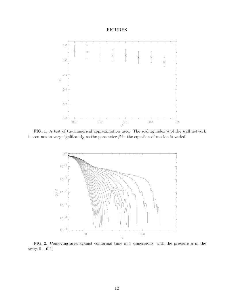
To verify the suitability of the numerical method used we ran a suite of simulations forD = 3 where β is increased in steps of 0.1 from zero and α is adjusted according to Eq.(6). Inorder for the domain wall to be resolvable, it should occupy at least one (preferably several)lattice spacing(s); this corresponds to a limiting value of β ≃ 0.66 in our simulations. Infigure 1 we show that the exponent ν in Eq.(13) does not change significantly as β is increasedup to this value.2 Overall the gross features of the evolution appear to be insensitive to thenumerical approximation used; in particular the onset and termination of the scaling regimeare not dependent on β. This adds further weight to the conclusion of Press et al. that thereis no difference between the dynamics of ‘real’ walls which have constant physical thickness,and the ‘artificial’ walls in these simulations which have constant comoving thickness.

A. Pressure

A well known way [10,24] to evade the causal limit on the disappearance of the domainwalls is to include a pressure term in the potential, viz.

V (φ) = V0

(

φ2

φ20

− 1

)2

+ µφ

φ0

, (15)

The dynamics is now expected to be dominated by two competing forces, the surface tensionσ/R where R ≃ aξ is the radius of curvature of the wall structure, and the pressure which

2There appears to be a small systematic trend of decreasing ν with increasing β. Although

not statistically significant, this may just reflect the increasing efficiency of the area measuring

algorithm at picking up small bubbles at late times, as β is increased.

5

is equal to the differences in energy density of the two minima of the potential, δV . Thenwe expect simple scaling behaviour (12) until some conformal time ηc at which the pressurebecomes comparable to the surface tension, and the wall network disappears exponentiallyfast. Now ηc is given by

σa(η0)

(ηc − η0)a(ηc)= δV , (16)

where the subscript 0 indicates the value at the begining of the evolution. In the presentcase we are scaling the fields with time so as to remove factors of a and set η0 = 1 so thisequation will reduce simply to

σ

ηc= 2µ . (17)

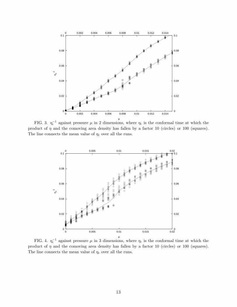
We display this behaviour in figure 2, where the comoving area density is plotted againstconformal time for several choices of ε. As expected, there is an exponential fall-off from thescaling regime at some value of ηc which decreases with increasing µ. The ‘bounces’ in thecurves occur as the bubbles of the disfavoured vacuum collapse and radiate away the energycontained in the walls in the form of Goldstone bosons; as noted earlier [25] a large fractionof the energy is lost in a few bounces. The relation between µ and ηc is shown in figures 3and 4, which show excellent agreement with the expected behaviour (17) to within a factorof 2. (Here ηc is defined as the value of η at which the product η(A/V ) has fallen off bysome factorm taken here to be 10 and 100 for illustration.) The actual rate of the decay ofthe wall network after the exponential decay has set in is hard to measure. We find herethat assuming a behaviour of form (A/V )c ∼ η−1 exp[−κ(µη)n] with κ some constant, n is≈ 2 ± 1 (D = 2) and ≈ 3 ± 1 (D = 3).

The implication of this is that we can regard the walls as simply disappearing as aconsequence of the difference in energy between the two minima of the potential δV at acorrelation length Rc = σ/δV (in physical, not comoving, units), where again the constantof proportionality is around unity. Hence, if we have walls forming at the electroweak scaleand we require that they disappear before nucleosynthesis [12], we find

δV

σ>

1

1010 cm∼ 10−24 GeV , (18)

in good agreement with previous estimates made from physical arguments as to the time ofpressure domination [10] and 2-dimensional thin wall simulations [26].

B. Bias

Next we consider the possibility of a deviation from scaling behaviour due to a biased

initial probability distribution. For concreteness we consider the Z2 case where there areonly two distinct vacuua and we generate the initial configuration with a probability

p+ = 0.5 + ε (19)

that each initial domain is in the + phase, where ε > 0. A similar exercise has beenperformed recently by Coulson, Lalak and Ovrut [18] who find that the domain wall network

6

then evolves much more rapidly than in the usual case of Eq.(12), and the favoured domainrapidly dominates the universe. Such a scenario is interesting because a bias in a light scalarfield which is not in thermal equilibrium can be generated naturally by a previous epochof inflation. Other possible ways in which a scalar field is more likely to find itself in oneminimum than the other are if the symmetry is approximate, so that the two minima are notexactly degenerate, or if the symmetry breaking occurs through some intermediate phasewhich allows one minimum to be preferentially populated.

The evolution is shown in figure 5, where we plot comoving area density against conformaltime for several choices of ε, ranging upto 0.03. Typically, the behaviour is similar to theusual case of no bias, with an exponential decay of the comoving energy density startingat some critical timescale ηc. (For η <∼ 10 the behaviour is unphysical since ξ is less thanthe domain wall thickness (here scaled to be 5), while for η >∼ 100, ξ is approaching thephysical size of the box, and hence the behaviour is again unphysical.) Notice that the wallnetwork dissipates rapidly as ε is increased above zero, as was also found in ref. [18]. (Againwe see the ‘bounces’ associated with the radiating away of the energy contained in the wallnetwork.)

Hindmarsh [17] has recently made an analytic study of biased domain walls. He considersthe evolution of the domain walls in terms of a scalar field constructed so that its zeroscorrespond to the locations of the domain walls, and whose evolution can be calculated interms of Gaussian average field configurations; the expectation for the wall surface areadensity in D dimensions is

(A/V ) ∼ 1

ηexp

(

−κε2ηD)

, (20)

where κ is some constant which should, in our units, be of order unity. The above resultwas obtained using rather sophisticated techniques but we can derive it from a much simpler(but perhaps less trustworthy) counting argument. We consider the wall evolution to proceedin such a way that the universe naturally divides itself up into domains of size ξ≃vη (incomoving coordinates). Such domains have been causally connected, and so have had timeenough to organize themselves to be either all + or all −. Hence we can see that thecomoving area density in the absence of bias will behave as (A/V ) ≃ ξ−1 ≃ (vη)−1 asexpected. We can now examine the behaviour of the comoving area density in the morecomplicated situation when there is a bias. Now we expect a domain of conformal size ξ tobecome a + domain if most of its ξ3 subdomains are +, and a − domain otherwise. (Wehave normalized so that the size of the initial domains is unity.) If the probability of eachsubdomain entering the positive minimum is p+, the probability for the whole domain to be− is given by a sum over values of a Poisson distribution which can, in any interesting case,be taken to be a Gaussian integral, viz.

P(domain of N sites, mostly −) = erf

(

N − N/2

σN

)

= erf(√

2ε√

N) , (21)

where N = (0.5+ε)N is the mean number of + sites and σN =√

N is the standard deviation.Here the Gaussian integral erf(x) ≡

∫

∞

x dt e−t2/2/√

2π can be adequately approximated forlarge x by

7

erf(x) =1

x√

2πe−x2/2. (22)

We see that for a box with ξ sites, the probability given in Eq.(21) is just erf(√

2εξD/2)and hence we expect exactly the exponential behaviour shown earlier in Eq.(20). The extrafactor of (ξD/2)−1 is cancelled by a combinatoric factor from the many different ways inwhich we can lay down our domains upon the overall network. This uses the fact that acluster containing N sites will typically scale as N1/2, using the results of percolation theoryas recently applied to similar problems in cosmology [27].

To verify this behaviour, we define ηc to be the conformal time at which the productη(A/V ) has decreased by some substantial factor, which we choose to be 10 and 100 forillustration. The values of η−D/2

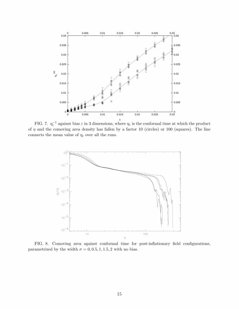
c are plotted against ε for both 2 and 3 dimensions infigures 6 and 7 and we find good agreement with the theoretical prediction of a straightline. Note that for both cases, we have cut off the figures at η ≃ 10 since before thisconformal time the domain wall network is not yet fully formed. We also expect unreliableresults when η reaches 100 or 1000 in three and two dimensions respectively, since then thecorrelation length is approaching the size of our whole simulation. While we can measurethe relationship between ηc and the bias ε, it is again harder to measure the actual rate ofthe exponential fall off, i.e. the exponent of η in the exponential. We find this exponent tobe ≈ 1 − 2 (D = 2) and ≈ 2 − 3 (D = 3), in acceptable agreement with theory.

Therefore we can, for cosmological purposes, regard the wall evolution as being in theKibble scaling regime for early times, and modelled subsequently by an exponential fall offat some conformal time ηc, which will lead to an almost immediate collapse of the wallnetwork. The required value of ε is readily calculable in three dimensions from

ε =

(

ηc

η0

)−3/2

=(

T0

Tc

)−3/2

, (23)

where ηc (Tc) is the scale factor (temperature) at the time of disappearance and η0 (T0) atthe time of domain formation. (Note that here we put κ ≃ 1 from our simulation result.)For example, in the event of wall formation at the weak scale of order 100 GeV, with therequirement that the walls disappear before the nucleosynthesis era which starts at ∼ 1 MeV[12], we find that ηc/η0 ∼ 105, and hence that the bias in the initial probability distributionmust be of order 10−8 or greater. However if the walls form subsequent to reheating followinginflation, at an energy scale of say 106 GeV, the bias need only be about 10−14.

C. Realistic Field Configurations

It is usually assumed [5] that following cosmological discrete symmetry breaking in ascalar field, the field values will be uncorrelated on scales larger than the causal (particle)horizon, so the degenerate vacuua will be populated with equally probability. However, aprior period of cosmological inflation can result in correlations on (apparently) super-horizonscales if the field is sufficiently weakly coupled so as not to be in thermal equilibrium. This isbecause quantum fluctuations during inflation (with Hubble parameter H) will induce long-wavelength fluctuations in all scalar fields with mass m ≪ H on spatial scales k−1 ≫ H−1

8

[14]. For a minimally coupled field with vanishing potential (e.g. a (pseudo-) goldstone bo-son), this leads to the formation of a classical inhomogeneous field, with gaussian probabilitydistribution [28]

P(φ) ∝ exp

[

−(φ − φk)2

2σ2k

]

, σ2k ≃ H2

4π2

∫ kc

kd ln k . (24)

where φk is the mean value of the field averaged over a domain of size k−1 and kc is aneffective ultraviolet cutoff imposed by physical considerations (dependent on the natureof the field). Since inflation blows up the scale factor exponentially fast, this provides anatural mechanism for bias since the global ensemble average of φ may not be realized evenover regions as big as our present universe. During the post-inflationary phase, the abovedistribution (24) averaged over a chosen scale thus becomes skewed [15]. We parametrize thisfor the Z2 case by drawing probabilities for populating the two vacuua from the distribution

P(φ) =1√2πσ

[

(0.5 − ε)e−(φ+1)2/2σ2

+ (0.5 + ε)e−(φ−1)2/2σ2]

, (25)

where ε is the effective bias over the chosen scale. (Presumably its value can be calculatedin principle if the field and inflationary parameters are specified.) In figures 8 and 9 weshow the comoving area density plotted against conformal time for several choices of σ withε = 0, 0.005. Surprisingly, the exponential fall-off from the scaling regime appears to bequite insensitive to the width of the probability distribution. This supports the suggestion[15] that this is an efficient way to eliminate the domain wall network.

IV. CONCLUSIONS

We have considered two possible ways in which a cosmological domain wall networkcan be made unstable. The first of these is that of pressure, i.e. a small breaking of thedegeneracy between the minima. The physical implications of this are well understood andwe have simply confirmed numerically the usual argument [10] that when the typical domainsize R has grown to a critical value Rc, the wall energy density decays exponentially fast,so the network disappears essentially instantaneously. The value of Rc is

Rc =σ

δρ, (26)

where σ is the wall surface energy density and δρ is the difference in energy density betweenthe two minima. (There may be an additional effect due to the bias induced at the phasetransition by the energy difference between the two minima.)

The second mechanism is that of bias, where the initial field configuration is not sym-metric between the various minima of the potential. Here we confirm previous analytical[17] and numerical [18] studies which predict an exponential decay in the energy densitywith a characteristic conformal time ηc. This is an attractive solution to the domain wallproblem if we can find a natural mechanism to bias the initial distribution, particularly sincewe find the evolution to be insensitive to the width of the distribution. Since such a biasmust appear on (apparently) causally disconnected scales, it can only occur if either the

9

minima are genuinely inequivalent (and so have non-degenerate energy densities) or else ifwe are in a post-inflationary phase in which the field has correlations on super-horizon scales.This will allow the universe to more efficiently organise itself into one preferred minimumeverywhere, thus enabling the wall network to decay away. Now an initial field configurationwith correlations on all wavelengths can be characterized by an effective bias ε(R) averagedover a box of size R, as high frequency modes will average out to zero. We have seen thata region of size R will decay away exponentially after a conformal time ηc(R) ∼ ε(R)−D/2.For a radiation dominated universe, the time t(R) at which the domain will decay is then

t(R) ∼ ε(R)−3 , (27)

which must grow more slowly than R to ensure that the ordinary causal scaling bound is ex-ceeded. Hence for bias to provide a realistic means of eliminating wall networks through aninitially non-equilibrium field distribution, we must have that ε(R) falls off with R moreslowly than R−1/3. Since the spectrum of fluctuations from inflation is (nearly) scale-invariant, we may expect that the bias ε(R) does stay approximately constant with R,and hence that this mechanism provides a way of eliminating domain walls in fields whichare sufficiently weakly coupled so as not to be in thermal equilibrium.

ACKNOWLEDGMENTS

S.E.L. thanks CSN and KV (Sweden), ORS and OOB (Oxford) and the Sir RichardStapley Educational Trust (Kent), and S.S. thanks PPARC for support. We are grateful toSteven Abel, Mark Hindmarsh, Zygmunt Lalak and Graham Ross for helpful discussions andto the referee for prompting us to investigate in more detail the numerical method employed.

10

REFERENCES

[1] Ya.B. Zel’dovich, I.Y. Kobzarev and L.B. Okun, Sov. Phys. JETP 40, 1 (1975).[2] G. Dvali and G. Senjanovic, Phys. Rev. Lett. 74, 5178 (1995);

G. Dvali, A. Melfo and G. Senjanovic, Report No. SISSA 18/96/A [hep-ph/9601376].[3] S. Weinberg, Phys. Rev. D 9, 3357 (1974);

R.N. Mohapatra and G. Senjanovic, Phys. Rev. D 20, 3390 (1979).[4] G. Bimonte and G. Lozano, Phys. Lett. B366, 248 (1996), Report No. DFTUZ/96/11

[hep-th/9603201];G. Amelino-Camelia, Report No. OUTP-96-44P [hep-ph/9610262].

[5] T.W.B. Kibble, J. Phys. A9, 1387 (1976).[6] D. Stauffer, Phys. Rep. 54, 1 (1979).[7] D. Seckel, Inner Space–Outer Space, edited by E.W. Kolb et al. (University of Chicago

Press, 1986) p.367.[8] A. Vilenkin, Phys. Rep. 121, 263 (1985);

A. Vilenkin and E.P.S. Shellard, Cosmic Strings and other Topological Defects (Cam-bridge University Press, 1994).

[9] B. Holdom, Phys. Rev. D 28, 1419 (1983);B. Rai and G. Senjanovic, Phys. Rev. D 49, 2729 (1994).

[10] A. Vilenkin, Phys. Rev. D 23, 852 (1981);P. Sikivie, Phys. Rev. Lett. 48, 1156 (1982);F.W. Stecker, Phys. Lett. 143B, 351 (1984).

[11] J. Ellis et al., Phys. Lett. B176 (1986) 403.[12] S. Sarkar, Rep. Prog. Phys. 59, 1493 (1996).[13] S.A. Abel, S. Sarkar and P.L. White, Nucl. Phys. B 454 (1995) 663.[14] A. Vilenkin and L.H. Ford, Phys. Rev. D 25, 1231 (1982);

A.D. Linde, Phys. Lett. B 116, 335 (1982);A.A. Starobinsky, Phys. Lett. B 117, 175 (1982);S.-J. Rey, Nucl. Phys. B 284, 706 (1987).

[15] Z. Lalak, S. Thomas and B.A. Ovrut, Phys. Lett. B 306 (1993) 10.[16] S. Lola and G.G. Ross, Nucl. Phys. B 406 (1993) 452;

Z. Lalak, S. Lola, B. Ovrut and G.G. Ross, Nucl. Phys. B 434 (1995) 675.[17] M. Hindmarsh, Phys. Rev. Lett. 77, 4495 (1996).[18] D. Coulson, Z. Lalak and B. Ovrut, Phys. Rev. D 53, 4237 (1996).[19] L. Kawano, Phys. Rev. D 41, 1013 (1990).[20] J. Ipser and P. Sikivie, Phys. Rev. D 30, 712 (1984).[21] A. Albrecht and N. Turok, Phys. Rev. D 40, 973 (1989).[22] W.H. Press, B.S. Ryden and D.N. Spergel, Astrophys. J. 347, 590 (1989).[23] W.H. Press, B.S. Ryden and D.N. Spergel, Astrophys. J. 357, 293 (1990).[24] J.A. Frieman, G.B. Gelmini, M. Gleiser and E.W. Kolb, Phys. Rev. Lett. 60, 2101

(1988);G.B. Gelmini, M. Gleiser and E.W. Kolb, Phys. Rev. D 39, 1558 (1989).

[25] L.M. Widrow, Phys. Rev. D 39, 3576 (1989).[26] S.A. Abel and P.L. White, Phys. Rev. D 52, 4371 (1995).[27] Z. Lalak, B. Ovrut, S. Thomas, Phys. Rev. D 51, 5456 (1995).[28] A.D. Linde and D.H. Lyth, Phys. Lett. B 246, 353 (1990).

11

FIGURES

FIG. 1. A test of the numerical approximation used. The scaling index ν of the wall network

is seen not to vary significantly as the parameter β in the equation of motion is varied.

FIG. 2. Comoving area against conformal time in 3 dimensions, with the pressure µ in the

range 0 − 0.2.

12

0

0.02

0.04

0.06

0.08

0.1

0 0.002 0.004 0.006 0.008 0.01 0.012 0.0140

0.02

0.04

0.06

0.08

0.10 0.002 0.004 0.006 0.008 0.01 0.012 0.014

η c-1

µ

FIG. 3. η−1c against pressure µ in 2 dimensions, where ηc is the conformal time at which the

product of η and the comoving area density has fallen by a factor 10 (circles) or 100 (squares).

The line connects the mean value of ηc over all the runs.

0

0.02

0.04

0.06

0.08

0.1

0 0.005 0.01 0.015 0.020

0.02

0.04

0.06

0.08

0.10 0.005 0.01 0.015 0.02

η c-1

µ

FIG. 4. η−1c against pressure µ in 3 dimensions, where ηc is the conformal time at which the

product of η and the comoving area density has fallen by a factor 10 (circles) or 100 (squares).

The line connects the mean value of ηc over all the runs.

13

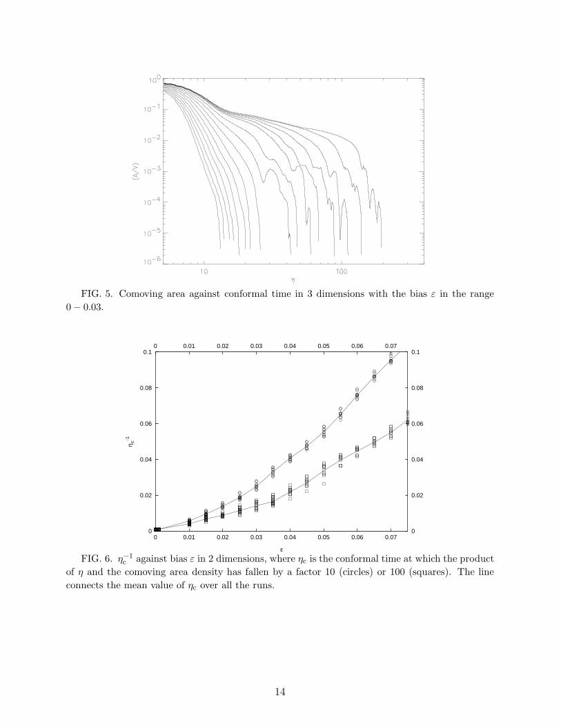
FIG. 5. Comoving area against conformal time in 3 dimensions with the bias ε in the range

0 − 0.03.

0

0.02

0.04

0.06

0.08

0.1

0 0.01 0.02 0.03 0.04 0.05 0.06 0.070

0.02

0.04

0.06

0.08

0.10 0.01 0.02 0.03 0.04 0.05 0.06 0.07

η c-1

ε

FIG. 6. η−1c against bias ε in 2 dimensions, where ηc is the conformal time at which the product

of η and the comoving area density has fallen by a factor 10 (circles) or 100 (squares). The line

connects the mean value of ηc over all the runs.

14

0

0.005

0.01

0.015

0.02

0.025

0.03

0.035

0.04

0 0.005 0.01 0.015 0.02 0.025 0.030

0.005

0.01

0.015

0.02

0.025

0.03

0.035

0.040 0.005 0.01 0.015 0.02 0.025 0.03

η c-3

/2

ε

FIG. 7. η−1c against bias ε in 3 dimensions, where ηc is the conformal time at which the product

of η and the comoving area density has fallen by a factor 10 (circles) or 100 (squares). The line

connects the mean value of ηc over all the runs.

FIG. 8. Comoving area against conformal time for post-inflationary field configurations,

parametrized by the width σ = 0, 0.5, 1, 1.5, 2 with no bias.

15

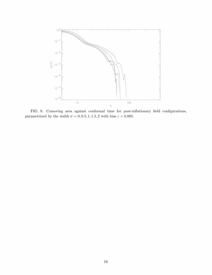
FIG. 9. Comoving area against conformal time for post-inflationary field configurations,

parametrized by the width σ = 0, 0.5, 1, 1.5, 2 with bias ε = 0.005.

16