arX

iv:h

ep-p

h/02

0503

6v2

3 M

ay 2

002

ANL-HEP-PR-02-033July 22, 2017

CHIRALITY VIOLATION IN

QCD REGGEON INTERACTIONS∗

Alan. R. White†

High Energy Physics DivisionArgonne National Laboratory

9700 South Cass, Il 60439, USA.

Abstract

The appearance of the triangle graph infra-red axial anomaly in reducedquark loops contributing to QCD triple-regge interactions is studied. In a dis-persion relation formalism, the anomaly can only be present in the contributionsof unphysical triple discontinuities. In this paper an asymptotic discontinuityanalysis is applied to high-order feynman diagrams to show that the anomalydoes indeed occur in sufficiently high-order reggeized gluon interactions. Thereggeon states involved must contain reggeized gluon combinations with thequantum numbers of the anomaly (winding-number) current. A direct con-

nection with the well-known U(1) problem is thus established. Closely related

diagrams that contribute to the pion/pomeron and triple pomeron couplings incolor superconducting QCD are also discussed.

∗Work supported by the U.S. Department of Energy, Division of High Energy Physics,Contracts W-31-109-ENG-38 and DEFG05-86-ER-40272

†arw@hep.anl.gov

1. INTRODUCTION

It is commonly believed that non-perturbative quark chirality transitions playan important role within the QCD bound-state S-Matrix. Assuming that the theory

can be quantized via a suitably defined euclidean path-integral‡, the chirality transi-tions are understood as originating from gauge-dependent non-perturbative classicalsolutions with non-trivial topology. Field configurations of this kind produce zeromodes of the Dirac operator which[2] prevent the gauge-invariant separation of mass-less fermion fields into right- and left-handed components that separately create parti-cles and antiparticles. The resulting violation of axial charge conservation is describedby the anomalous divergence equation for the U(1) axial current. While many conse-

quences of chirality violation are understood, for example the generation[3] of a mass

for the η′, it’s full significance in determining the non-perturbative massless S-Matrixis far from understood. In particular, the role of chirality violation due to topologicalgauge fields in chiral symmetry breaking is the subject of much debate[4, 5].

In this paper, and a companion paper[6], we provide a completely differentunderstanding of chirality transitions in the massless, high-energy, QCD bound-stateS-Matrix. No mention is made of euclidean path-integral quantization or topologicalfields. Rather, as we explain further below, our arguments are based directly on thesingularity structure of high-order feynman diagrams that contribute to the high-energy scattering of bound-states.

It is well established[7] that when the gauge symmetry of QCD is sponta-

neously broken general high-energy limits (multi-regge limits) of quark and gluonamplitudes are described perturbatively by reggeon diagrams in which the reggeonsare simply massive, reggeized, gluons and quarks. Both t- and s- channel unitarityare satisfied. Reggeon interactions are described, in general, by “reduced” feynmandiagrams, obtained from underlying diagrams by placing some propagators on-shell.It is important, however, to distinguish two kinds of interaction vertices. The simplestkind are those that describe the repeated interaction of reggeons “propagating” ina single reggeon channel (for which there is only one overall transverse momentum).The well-known BFKL kernel is, essentially, an example of this kind of vertex. Thesecond kind are the vertices that couple different reggeon channels, the simplest beingthe triple-regge vertices[8] that couple three reggeon channels - each carrying a sep-arate transverse momentum. In the massless theory such vertices should contain thecouplings of bound-state reggeons (e.g. pions and nucleons) together with their cou-plings to the physical pomeron. Effectively, therefore, vertices of this kind determinethe bound-states of the theory and their high-energy scattering amplitudes.

‡We note, though, that the elimination of unphysical degrees of freedom remains an unsolvedproblem[1].

1

There are, of course, no axial-vector currents in the QCD interaction but in thereduced diagrams providing the crucial triple-regge vertices, components of an axial-vector interaction can appear. Therefore, we have suggested[10] that, in sufficientlyhigh orders, chirality violation due to the infra-red triangle anomaly should appearin reggeized gluon interactions of this kind. The purpose of this paper is to finallyestablish that this is the case. It is necessary, however, to study very high-orderdiagrams.

We have long believed[9] that the massless, bound-state, multi-regge, S-Matrixshould be obtainable from the massive reggeon diagrams once the infra-red role ofthe chiral anomaly is determined. In previous papers we have outlined[11, 12] how

(appropriately regularized) anomaly interactions can be the essential element that, incombination with the infra-red divergences of the massless limit, produce the “non-perturbative” properties of confinement and chiral symmetry breaking. We arguedthat, while the anomaly interactions cancel when the scattering states are perturba-tive quarks and gluons, for compound multiregge states with an appropriate infra-redcomponent such interactions dominate and infra-red divergences self-consistently pro-duce the bound-state S-Matrix. However, to demonstrate this via the construction ofa full set of multi-regge amplitudes is a complicated project which, of necessity, willinvolve much abstract multi-regge theory. While this construction is still our eventualgoal, as an intermediate step, we have first developed, in the companion paper to this,a calculational method that demonstrates the dynamical role of the anomaly whileavoiding the (little known) multi-regge formalism as much as possible. Light-coneproperties of the anomaly are heavily exploited and we are able to show how boththe U(1) and chiral flavor anomaly play essential roles.

By studying the interaction of (infinite momentum) axial currents we show[6]

that, when the SU(3) gauge symmetry is partially broken to SU(2), U(1) anomalyinteractions combine with couplings due to the flavor anomaly to produce an infra-reddivergent amplitude for the scattering of Goldstone boson “pions” and “nucleons”.The flavor anomaly produces the pion particle poles, while the U(1) anomaly producesthe high-energy coupling of the pions to the exchanged pomeron. After the divergenceis factorized off, as a wee gluon condensate within the scattering states, the remainingamplitudes have both confinement and chiral symmetry breaking. (The wee gluoncondensate can be identified directly with the infra-red component of multi-reggestates that appears in the multi-regge program.) It is apparent that the nature ofthe pomeron is crucially dependent on chiral symmetry breaking. We anticipate thatrestoration of full SU(3) gauge symmetry will result from randomization of the SU(2)

condensate within SU(3) and that the Critical Pomeron[13] will appear.

The main focus of this paper will be on multigluon reggeon inteactions thatare most directly relevant to the general multi-regge program and the pomeron in-teractions that emerge. However, as we briefly describe at the end of this paper, the

2

multiquark/gluon interaction that provides the pion/pomeron coupling in [6] is veryclosely related to the reggeized gluon interactions that we study. We will establish,remarkably perhaps, that for the anomaly to appear the reggeon states involved mustcontain gluon combinations with the quantum numbers of the anomaly (winding-

number) current. The conventional U(1) problem is, therefore, clearly encountered.We will concentrate on isolating the anomaly via infra-red properties. Nevertheless,although we will discuss this only briefly at a few key points, we expect the infra-redphenomena we discuss to be connected to “ultra-violet” reggeon interaction problems(involving momenta flowing around an internal quark loop that are comparable in

magnitude to large external momenta) where short-distance interactions of the wind-ing number current appear directly. That the anomaly is a high-order, many gluon,phenomenon is not surprising if the anomaly current, containing a product of threegluon fields, has to be involved.

Properties of the triangle diagram are discussed in detail in the companionpaper[6], where a complete set of the the relevant references is given. For our presentpurposes we note that the massless axial-vector graph has an infra-red divergencethat involves a zero four-momentum fermion propagator. Both the “particle” and“antiparticle” poles of this propagator contribute to the divergence. The couplingat one end of the propagator can be viewed as the vertex for production of theparticle while simultaneously (and symmetrically) that at the other end describes theproduction of the antiparticle. If the zero momentum propagator describes a physicaltransition it implies that there is, necessarily, an accompanying “spectral flow” of thefermion energy spectrum so that the production of the antiparticle (or the particle)corresponds to the production of a Dirac hole state, i.e. the absorption of a particle(antiparticle). In this way, the transition is understood as a “chirality transition”

In Minkowski space the Dirac zero modes due to topological gauge fields doindeed produce[2] spectral flow (with time) of the eigenvalues of the correspond-

ing (gauge-dependent) “Hamiltonian”. However, since there is no complete non-perturbative Hamiltonian formalism for massless QCD, there is no understanding of

the full consequences of spectral flow§. The phenomenon we see is, arguably, the min-imum spectral flow that could be present (if there is any). Zero momentum fermion

states identified initially as a particle (within a boundstate) can evolve with timeinto a filled vacuum state of the corresponding Dirac sea and, similarly, filled vacuumstates can evolve into particles. (The existence of stable bound states and physi-

cal scattering processes in such an environment is clearly far from trivial!). In ouranalysis spectral flow of this kind is directly introduced by the appearance of thetriangle graph infra-red divergence in reggeized gluon interactions. It is interesting

§The conventional wisdom is probably that strong coupling confinement effects overwhelm suchphenomena altogether. As we have emphasized elsewhere, we expect our discussion to apply to aweak coupling version of massless QCD in which there is, effectively at least, an infra-red fixed point.

3

that a related phenomenon has already been encountered in next-to-leading ordercalculations[14] of the high-energy scattering of massless gluons. A massless gluontriangle diagram occurs in the effective vertex for reggeized gluon exchange and pro-duces a “particle/antiparticle transition” that for gluons is simply an unanticipatedhelicity transition.

A reggeon interaction vertex can be obtained by calculating the contributionof Feynman diagrams to the simplest multi-regge limit in which the vertex appears.In [10] we distinguished two methods for calculating multi-regge amplitudes - thedirect calculation of diagrams in light-cone co-ordinates and the calculation of mul-tiple asymptotic discontinuities with the subsequent use of an asymptotic dispersionrelation. Although, the two methods should ultimately produce the same results, di-rect light-cone calculations are impractical for the problem we are discussing. This isbecause of the large number of diagrams that could contribute and because the com-plexity of the diagrams makes a full discussion of whether or not integration contoursare truly trapped, in the asymptotic limits involved, very difficult. Consequently theasymptotic dispersion relation method has to be used. In this paper, therefore, wedevelop methods aimed at directly calculating multiple asymptotic discontinuities.

The form of the asymptotic dispersion relation for a given multi-regge pro-cess is determined by the possible asymptotic multiple discontinuities that satisfythe Steinmann relation property (that the discontinuities occur in non-overlapping

invariant channels). Such discontinuities are explicitly reflected in the analytic struc-ture of asymptotic amplitudes provided by multi-regge theory and, conversely, usingthe dispersion relation, multi-regge amplitudes can be calculated directly from thediscontinuities. In [6] we described how the appearance of the anomaly pole in theelementary three current amplitude could be understood as due to an unphysicaltriangle landau singularity appearing (from an unphysical sheet) at the edge of thephysical region. Correspondingly, the crucial feature of the high-order amplitudesthat produce reggeon interactions containing the anomaly is the presence of unphysi-cal multiple discontinuities that satisfy the Steinmann relation property and approachphysical scattering regions only asymptotically. (This implies that they correspondto contour trappings that would be very difficult to demonstrate using direct light-cone calculations.) Discontinuities of this kind are present in complex (imaginary

momentum) parts of the asymptotic region for sufficiently complicated many-particle

multi-regge processes, the simplest of which is the full triple-regge region[8] that westudy in this paper. Because they are in non-overlapping channels these discontinu-ities can (and must) consistently appear in the asymptotic amplitudes that describealso the real physical region behavior.

The familiar amplitudes that appear in multi-regge production processes (such

as those that contribute to the BFKL equation[7]) do not contain unphysical multiplediscontinuities. Rather they contain only multiple discontinuities that are naturally

4

interpreted as due to a succession of physical region on-shell scattering processes. (Thenecessity for a physical time-ordering of such processes then determines the absenceof overlapping channel discontinuities.) Because physical region multiple discontinu-ities involve only physical amplitudes and physical intermediate states, when theyare calculated using the perturbative amplitudes of the massless theory, they can notcontain chirality transitions associated with particle/antiparticle ambiguities. There-

fore, when only production processes are involved (i.e. at what we might call the

BFKL level of multi-regge theory) there is no possibility for “chirality violation”.

A priori, there is no reason why unphysical multiple discontinuities should notcontain potential chirality transitions when calculated perturbatively. Nevertheless,the occurence of the infra-red anomaly within such discontinuities is very subtle. Thedivergence is produced by a quark loop that reduces to a triangle by the placing ofmany propagators on-shell. Of the three propagators associated with the trianglediagram, one must carry the zero momentum that allows a chirality transition whilethe other two carry the same light-like momentum. The additional on-shell propa-gators have to be associated with a triple discontinuity in such a way that (when all

transverse momenta are zero) they also can all carry the same light-cone momentum

(relative to the direction of the loop momentum). It is obvious that this requirementcan not be satisfied by a physical triple discontinuity and, in fact, it is very difficultto satisfy. (As we briefly discuss towards the end of this paper, this difficulty is likelyto be closely related to the complexity involved in having local interactions of theanomaly current appear in the ultraviolet region of reggeon interaction vertices.) In-

deed, we will see that by itself this requirement is sufficient to ensure that (in the

obtained reggeon interaction) at least three reggeons are present in each reggeon chan-nel. Requiring that the spin structure that generates the anomaly also be present,then further restricts the contributing triple discontinuities to those originating froma small class of feynman diagrams. The discontinuities involved are truly unphysicalin that they correspond to three “asymptotic pseudothresholds” (or, in more tech-

nical S-Matrix language, “mixed α singularities”) each of which contains particles

(effectively) going in opposite time directions. Not surprisingly, though, this providesjust the right circumstances for the anomaly to appear.

As we noted above, the obtained reggeon interactions are of such high orderthat the minimum circumstances in which they can occur (between color zero reggeon

states) is when each of the states involved carries the quantum numbers of the U(1)

anomaly current. The lower-order diagrams considered in [10] remain valuable todiscuss for illustrative processes but the analysis within this paper shows that they areessentially irrelevant. We do not give any detailed discussion of further cancelationsamongst the diagrams we consider. We note, however, that the signature rule of [10]implies that the full vertex for three reggeon states, each of which carries the quantumnumbers of the U(1) anomaly current, must vanish. In the pion/pomeron vertex

5

obtained in [6] there are, in addition to the three gluon reggeons, a quark/antiquarkpair in the pion, and an additional reggeon in the pomeron. In the triple pomeronvertex, which we also briefly discuss, there is an additional reggeon in each channel. Infollowing papers we hope to lay out the details of the construction of the full multi-regge S-Matrix alluded to above. For the moment we note only that triple-reggeinteractions of the kind we consider here will contribute generally to the vertices andinteractions of the reggeon bound states that emerge and refer to the brief discussionin [10], and also to the outline in [12], for more details.

6

2. MULTIPLE DISCONTINUITIES AND THE

STEINMANN RELATIONS.

2.1 Physical Region Discontinuities

The Steinmann relations originated in axiomatic field theory[15]. They (es-

sentially) describe the restrictions that the time-ordering of interactions places on thecombinations of intermediate states that can occur in a scattering process. For on-shell S-Matrix amplitudes their significance is most immediately appreciated in theapproximation that we ignore higher-order Landau singularities and consider only thenormal threshold branch points (and stable particle poles) that occur in individualchannel invariants. The Steinmann relations then say that simultaneous thresholds(and/or poles) can not occur in overlapping channels. (Channels overlap if they con-

tain a common subset of external particles.) As a result an N -point amplitude has at

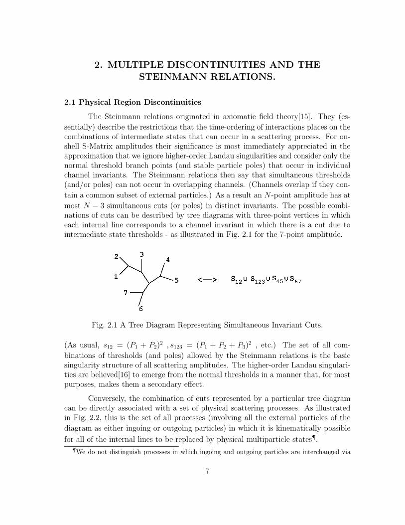
most N − 3 simultaneous cuts (or poles) in distinct invariants. The possible combi-nations of cuts can be described by tree diagrams with three-point vertices in whicheach internal line corresponds to a channel invariant in which there is a cut due tointermediate state thresholds - as illustrated in Fig. 2.1 for the 7-point amplitude.

Fig. 2.1 A Tree Diagram Representing Simultaneous Invariant Cuts.

(As usual, s12 = (P1 + P2)2 , s123 = (P1 + P2 + P3)

2 , etc.) The set of all com-

binations of thresholds (and poles) allowed by the Steinmann relations is the basicsingularity structure of all scattering amplitudes. The higher-order Landau singulari-ties are believed[16] to emerge from the normal thresholds in a manner that, for mostpurposes, makes them a secondary effect.

Conversely, the combination of cuts represented by a particular tree diagramcan be directly associated with a set of physical scattering processes. As illustratedin Fig. 2.2, this is the set of all processes (involving all the external particles of the

diagram as either ingoing or outgoing particles) in which it is kinematically possible

for all of the internal lines to be replaced by physical multiparticle states¶.¶We do not distinguish processes in which ingoing and outgoing particles are interchanged via

7

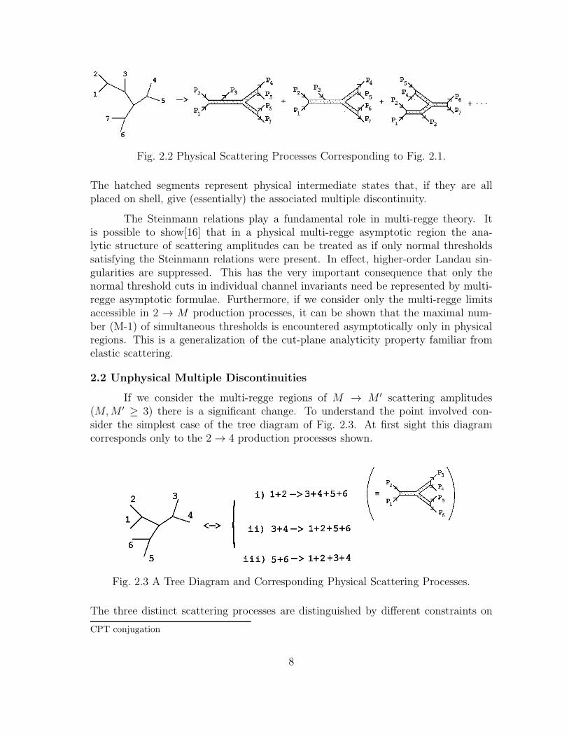
Fig. 2.2 Physical Scattering Processes Corresponding to Fig. 2.1.

The hatched segments represent physical intermediate states that, if they are allplaced on shell, give (essentially) the associated multiple discontinuity.

The Steinmann relations play a fundamental role in multi-regge theory. Itis possible to show[16] that in a physical multi-regge asymptotic region the ana-lytic structure of scattering amplitudes can be treated as if only normal thresholdssatisfying the Steinmann relations were present. In effect, higher-order Landau sin-gularities are suppressed. This has the very important consequence that only thenormal threshold cuts in individual channel invariants need be represented by multi-regge asymptotic formulae. Furthermore, if we consider only the multi-regge limitsaccessible in 2 → M production processes, it can be shown that the maximal num-ber (M-1) of simultaneous thresholds is encountered asymptotically only in physicalregions. This is a generalization of the cut-plane analyticity property familiar fromelastic scattering.

2.2 Unphysical Multiple Discontinuities

If we consider the multi-regge regions of M → M ′ scattering amplitudes(M,M ′ ≥ 3) there is a significant change. To understand the point involved con-sider the simplest case of the tree diagram of Fig. 2.3. At first sight this diagramcorresponds only to the 2 → 4 production processes shown.

Fig. 2.3 A Tree Diagram and Corresponding Physical Scattering Processes.

The three distinct scattering processes are distinguished by different constraints on

CPT conjugation

8

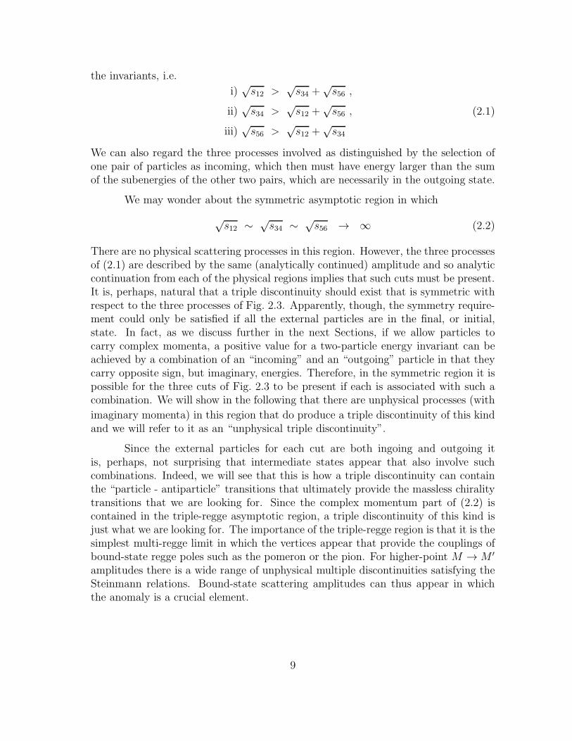
the invariants, i.e.

i)√s12 >

√s34 +

√s56 ,

ii)√s34 >

√s12 +

√s56 ,

iii)√s56 >

√s12 +

√s34

(2.1)

We can also regard the three processes involved as distinguished by the selection ofone pair of particles as incoming, which then must have energy larger than the sumof the subenergies of the other two pairs, which are necessarily in the outgoing state.

We may wonder about the symmetric asymptotic region in which

√s12 ∼ √

s34 ∼ √s56 → ∞ (2.2)

There are no physical scattering processes in this region. However, the three processesof (2.1) are described by the same (analytically continued) amplitude and so analyticcontinuation from each of the physical regions implies that such cuts must be present.It is, perhaps, natural that a triple discontinuity should exist that is symmetric withrespect to the three processes of Fig. 2.3. Apparently, though, the symmetry require-ment could only be satisfied if all the external particles are in the final, or initial,state. In fact, as we discuss further in the next Sections, if we allow particles tocarry complex momenta, a positive value for a two-particle energy invariant can beachieved by a combination of an “incoming” and an “outgoing” particle in that theycarry opposite sign, but imaginary, energies. Therefore, in the symmetric region it ispossible for the three cuts of Fig. 2.3 to be present if each is associated with such acombination. We will show in the following that there are unphysical processes (with

imaginary momenta) in this region that do produce a triple discontinuity of this kindand we will refer to it as an “unphysical triple discontinuity”.

Since the external particles for each cut are both ingoing and outgoing itis, perhaps, not surprising that intermediate states appear that also involve suchcombinations. Indeed, we will see that this is how a triple discontinuity can containthe “particle - antiparticle” transitions that ultimately provide the massless chiralitytransitions that we are looking for. Since the complex momentum part of (2.2) iscontained in the triple-regge asymptotic region, a triple discontinuity of this kind isjust what we are looking for. The importance of the triple-regge region is that it is thesimplest multi-regge limit in which the vertices appear that provide the couplings ofbound-state regge poles such as the pomeron or the pion. For higher-point M →M ′

amplitudes there is a wide range of unphysical multiple discontinuities satisfying theSteinmann relations. Bound-state scattering amplitudes can thus appear in whichthe anomaly is a crucial element.

9

3. THE PHYSICAL REGION ANOMALY AND THE

TRIPLE-REGGE DISPERSION RELATION

3.1 The Triple Regge Limit and Maximally Non-Planar Diagrams

In our previous paper[10] we studied the full triple-regge limit[8] of three-to-three quark scattering. If we denote the initial momenta as Pi , i = 1, 2, 3, and thefinal momenta as −Pi′ = Pi + Qi, i = 1, 2, 3, the triple-regge limit can be realized,within the physical region, by taking each of P1, P2 and P3 large along distinct light-cones, with the momentum transfers Q1, Q2 and Q3 kept finite, i.e.

P1 → P1+ = (p1, p1, 0, 0) , p1 → ∞P2 → P+

2 = (p2, 0, p2, 0) , p2 → ∞P3 → P+

3 = (p3, 0, 0, p3) , p3 → ∞

q1 = Q1/2 → (q̂1, q̂1, q12, q13)

q2 = Q2/2 → (q̂2, q21, q̂2, q23)

q3 = Q3/2 → (q̂3, q31, q32, q̂3)

(3.1)

Momentum conservation gives a total of five independent q variables which, alongwith p1, p2 and p3, give the necessary eight variables. The definition of the triple-regge limit in terms of angular variables is given in [10]. For our present purposes theabove definition in terms of momenta will be sufficient. This will alow us to avoid theextra complication of defining helicity angles, helicity-pole limits etc. The asymptoticbehavior involved must hold for all complex values of the large momenta, includingthe additional physical regions reached by reversing the signs of the pi.

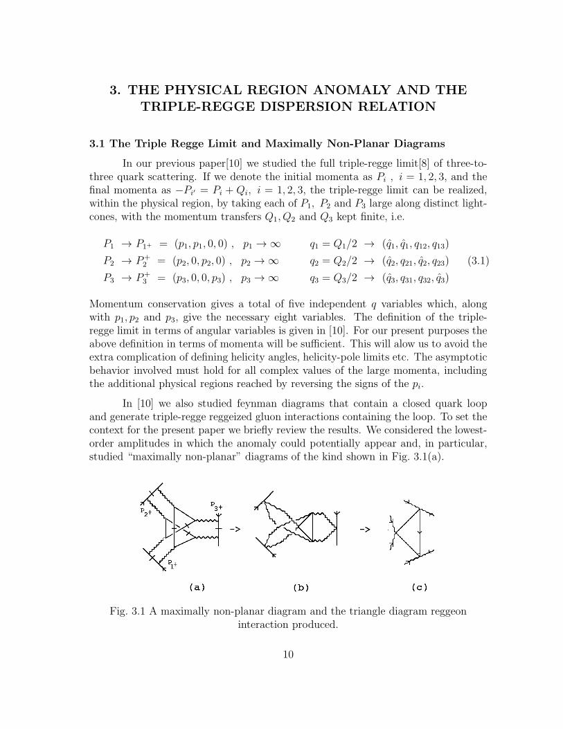
In [10] we also studied feynman diagrams that contain a closed quark loopand generate triple-regge reggeized gluon interactions containing the loop. To set thecontext for the present paper we briefly review the results. We considered the lowest-order amplitudes in which the anomaly could potentially appear and, in particular,studied “maximally non-planar” diagrams of the kind shown in Fig. 3.1(a).

Fig. 3.1 A maximally non-planar diagram and the triangle diagram reggeoninteraction produced.

10

(Throughout this paper we adopt the usual convention that solid and wavy linesrespectively represent a quark and a gluon. We have reversed the direction of P3

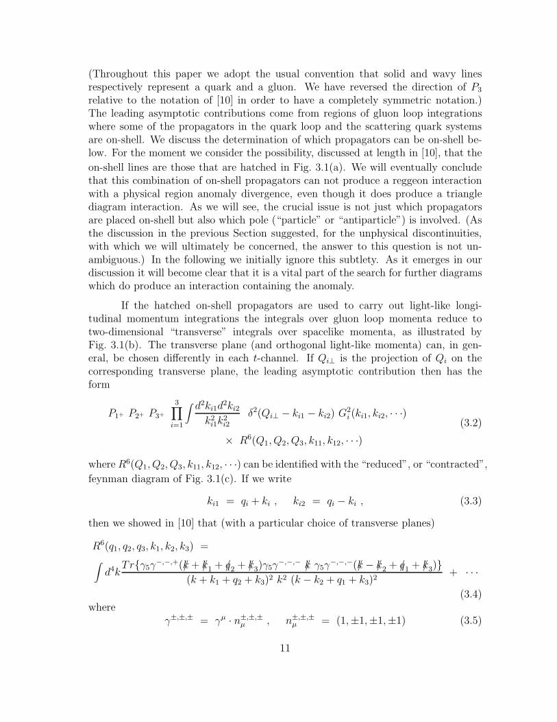
relative to the notation of [10] in order to have a completely symmetric notation.)The leading asymptotic contributions come from regions of gluon loop integrationswhere some of the propagators in the quark loop and the scattering quark systemsare on-shell. We discuss the determination of which propagators can be on-shell be-low. For the moment we consider the possibility, discussed at length in [10], that the

on-shell lines are those that are hatched in Fig. 3.1(a). We will eventually concludethat this combination of on-shell propagators can not produce a reggeon interactionwith a physical region anomaly divergence, even though it does produce a trianglediagram interaction. As we will see, the crucial issue is not just which propagatorsare placed on-shell but also which pole (“particle” or “antiparticle”) is involved. (Asthe discussion in the previous Section suggested, for the unphysical discontinuities,with which we will ultimately be concerned, the answer to this question is not un-ambiguous.) In the following we initially ignore this subtlety. As it emerges in ourdiscussion it will become clear that it is a vital part of the search for further diagramswhich do produce an interaction containing the anomaly.

If the hatched on-shell propagators are used to carry out light-like longi-tudinal momentum integrations the integrals over gluon loop momenta reduce totwo-dimensional “transverse” integrals over spacelike momenta, as illustrated byFig. 3.1(b). The transverse plane (and orthogonal light-like momenta) can, in gen-eral, be chosen differently in each t-channel. If Qi⊥ is the projection of Qi on thecorresponding transverse plane, the leading asymptotic contribution then has theform

P1+ P2+ P3+

3∏

i=1

∫

d2ki1d2ki2

k2i1k2i2

δ2(Qi⊥ − ki1 − ki2) G2i (ki1, ki2, · · ·)

× R6(Q1, Q2, Q3, k11, k12, · · ·)(3.2)

where R6(Q1, Q2, Q3, k11, k12, · · ·) can be identified with the “reduced”, or “contracted”,

feynman diagram of Fig. 3.1(c). If we write

ki1 = qi + ki , ki2 = qi − ki , (3.3)

then we showed in [10] that (with a particular choice of transverse planes)

R6(q1, q2, q3, k1, k2, k3) =∫

d4kTr{γ5γ−,−,+(k/ + k/1 + q/2 + k/3)γ5γ

−,−,− k/ γ5γ−,−,−(k/ − k/2 + q/1 + k/3)}

(k + k1 + q2 + k3)2 k2 (k − k2 + q1 + k3)2+ · · ·

(3.4)where

γ±,±,± = γµ · n±,±,±µ , n±,±,±

µ = (1,±1,±1,±1) (3.5)

11

The contributions to R6 not shown explicitly in (3.4) do not have a γ5 at all threevertices of the triangle diagram. As we will discuss again in Section 5, the particularγ-matrix projections appearing depend on the choice of transverse co-ordinates. If the

anomaly is present in R6, however, we expect it to be independent of this choice. Weshould emphasize that while we have written (3.4) as a function of four-dimensional

momenta, the ki are restricted to be two-dimensional spacelike momenta (plus longi-

tudinal components determined by the mass-shell conditions for the on-shell quarks)

and the qi have the restricted form given by (3.1). These restrictions play a cru-cial role in determining whether the anomaly can occur in a physical region reggeoninteraction.

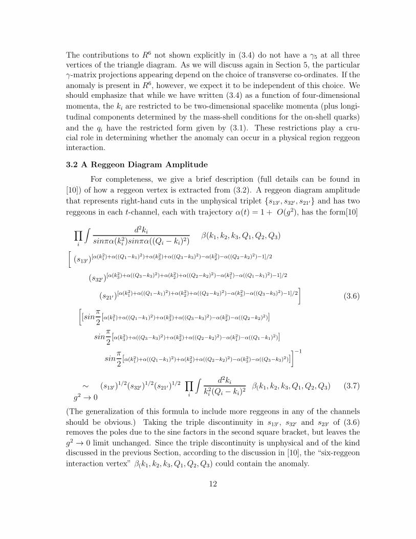
3.2 A Reggeon Diagram Amplitude

For completeness, we give a brief description (full details can be found in

[10]) of how a reggeon vertex is extracted from (3.2). A reggeon diagram amplitude

that represents right-hand cuts in the unphysical triplet {s13′ , s32′ , s21′} and has two

reggeons in each t-channel, each with trajectory α(t) = 1 + O(g2), has the form[10]

∏

i

∫

d2kisinπα(k2i )sinπα((Qi − ki)2)

β(k1, k2, k3, Q1, Q2, Q3)

[

(s13′)[α(k2

1)+α((Q1−k1)2)+α(k2

3)+α((Q3−k3)2)−α(k2

2)−α((Q2−k2)2)−1]/2

(s32′)[α(k2

3)+α((Q3−k3)2)+α(k2

2)+α((Q2−k2)2)−α(k2

1)−α((Q1−k1)2)−1]/2

(s21′)[α(k2

1)+α((Q1−k1)2)+α(k2

2)+α((Q2−k2)2)−α(k2

3)−α((Q3−k3)2)−1]/2

]

[

[sinπ

2[α(k2

1)+α((Q1−k1)2)+α(k2

3)+α((Q3−k3)2)−α(k2

2)−α((Q2−k2)2)]

sinπ

2[α(k2

3)+α((Q3−k3)2)+α(k2

2)+α((Q2−k2)2)−α(k2

1)−α((Q1−k1)2)]

sinπ

2[α(k2

1)+α((Q1−k1)2)+α(k2

2)+α((Q2−k2)2)−α(k2

3)−α((Q3−k3)2)]

]−1

(3.6)

∼g2 → 0

(s13′)1/2(s32′)

1/2(s21′)1/2

∏

i

∫

d2kik2i (Qi − ki)2

β(k1, k2, k3, Q1, Q2, Q3) (3.7)

(The generalization of this formula to include more reggeons in any of the channels

should be obvious.) Taking the triple discontinuity in s13′ , s32′ and s23′ of (3.6)removes the poles due to the sine factors in the second square bracket, but leaves the

g2 → 0 limit unchanged. Since the triple discontinuity is unphysical and of the kinddiscussed in the previous Section, according to the discussion in [10], the “six-reggeon

interaction vertex” β(k1, k2, k3, Q1, Q2, Q3) could contain the anomaly.

12

Writing

P1+P2+P3+ ≡ (s13′)1/2(s32′)

1/2(s21′)1/2 (3.8)

and comparing with (3.7) we see that it would be straightforward to identify (3.2)as a lowest-order contribution to such a reggeon diagram amplitude if the reducedfeynman diagram amplitude of Fig. 3.1(c) is identified as a reggeon vertex, i.e.

R6(Q1, Q2, Q3, k1, Q1 − k1, · · ·) ≡ β(k1, k2, k3, Q1, Q2, Q3) (3.9)

Note, however, that while the right-side of (3.8) clearly has a triple discontinuity in

{s13′ , s32′ , s21′}, the left-side does not. The equivalence of the two sides is only deter-

mined if higher-order terms in (3.6) appear and add to (3.2) in the appropriate man-ner. Such terms are contributed by what we refer to in the following as reggeization

diagrams. Note, also, that for parts of R6 (not including γ5 couplings) higher-orderterms would be expected to appear implying that, one or more of, the transverseintegrals in (3.2) should be interpreted as arising from the trajectory function terms

in (3.6). Such parts of R6 would then be interpreted as providing interaction verticesfor fewer reggeons.

The amplitude (3.4) representing Fig. 3.1(c) is the full four-dimensional trian-gle diagram amplitude except that special γ-matrices appear at the vertices and onlycombinations of (essentially) two-dimensional transverse momenta flow through the

diagram. It is shown in [10] that the γ-matrix couplings are appropriate to producethe anomaly but, as we discuss next, whether the necessary momentum configurationcan occur within a physical region and provide a physical region infra-red divergenceis a non-trivial and subtle question that depends crucially on the choice of propagatorpoles used to put lines on-shell.

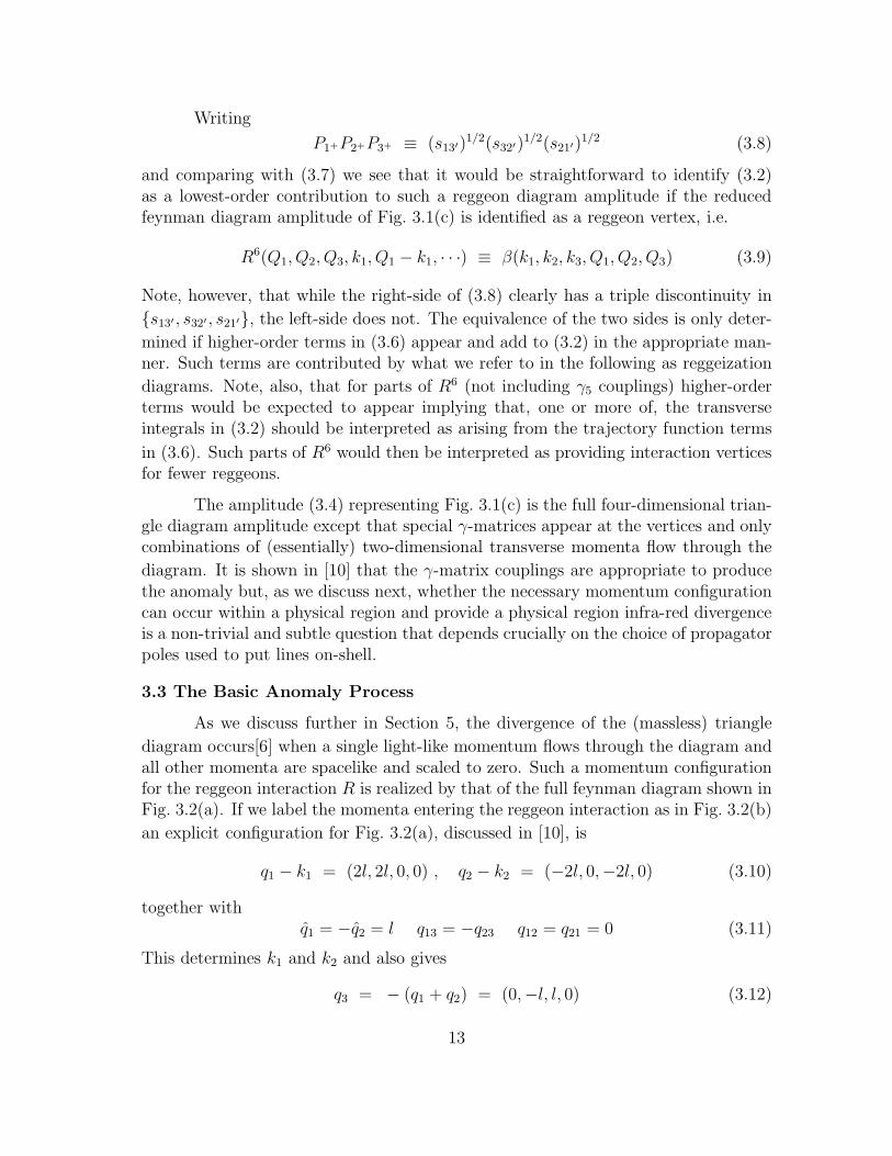
3.3 The Basic Anomaly Process

As we discuss further in Section 5, the divergence of the (massless) triangle

diagram occurs[6] when a single light-like momentum flows through the diagram andall other momenta are spacelike and scaled to zero. Such a momentum configurationfor the reggeon interaction R is realized by that of the full feynman diagram shown inFig. 3.2(a). If we label the momenta entering the reggeon interaction as in Fig. 3.2(b)

an explicit configuration for Fig. 3.2(a), discussed in [10], is

q1 − k1 = (2l, 2l, 0, 0) , q2 − k2 = (−2l, 0,−2l, 0) (3.10)

together withq̂1 = −q̂2 = l q13 = −q23 q12 = q21 = 0 (3.11)

This determines k1 and k2 and also gives

q3 = − (q1 + q2) = (0,−l, l, 0) (3.12)

13

If we then takek3 = l(0, 1− 2 cos θ , 1− 2 sin θ , 0) (3.13)

the light-cone momentum− 2l(1, cos θ, sin θ, 0) (3.14)

flows along the two vertical non-hatched lines in Fig. 3.2(b). It is straightforward tocheck that all three of the hatched lines are on mass-shell.

(a) (b)

Fig. 3.2 The basic anomaly process.

If spacelike momenta of O(q) are added to the momentum configuration (3.10)-(3.14)

and the limit q → 0 is taken, the anomaly divergence occurs. (We will discuss this in

more detail in Section 5.)

Apart from the reversal of direction for P3, the process represented by Fig. 3.2(a)

is what we called “the basic anomaly process” in [10]. The zero momentum quarkis produced by one “wee gluon” and absorbed by the other, allowing the chiralitytransition produced by the anomaly to compensate for a spin flip of the antiquark.Note, however, that when the wee gluons are massless, the scattering processs rep-resented by Fig. 3.2 is physical only when the quark and antiquark involved are alsomassless. In addition, as we noted in the Introduction (and discussed in more detail

in [6], the anomaly infra-red divergence involves both poles of the zero momentumquark propagator. Moreover, the vertices coupling to the propagator should, a priori,be symmetrically interpreted as describing either the simultaneous production of thetwo states in the propagator or their simultaneous absorption. When, as is the casein [6], the infra-red divergence analysis used to define physical states and amplitudesrequires that the massless scattering enter the physical region with the time order-ing implied by Fig. 3.2, the presence of a non-perturbative background gauge field iseffectively implied. The background field would be needed to produce the necessaryspectral flow at one vertex that is required to interpret the process as a chiralitytransition.

14

While the required mass-shell conditions are indeed satisfied by (3.10)-(3.14),

there is a problem. With the momenta given by (3.10)-(3.14), the energy component

of each of the three hatched lines in Fig. 3.2(b) has the same sign. Since the exchangedgluons carry only spacelike momenta, it is clear that this must be the case. We willsee that this is a very difficult configuration to obtain within a reggeon interaction.We can emphasize the problem by letting l → 0 while simultaneously making a boostaz(ζ) such that l cosh ζ = n is kept finite. (This is what is done in [6].) If we thentake all transverse momenta to zero, we obtain

q1 − k1 → (2n, 0, 0, 2n) , q2 − k2 → (−2n, 0, 0,−2n) (3.15)

and all the on-shell propagators carry the same light-like momentum (with respect to

the direction of the loop momentum). Effectively, then, the on-shell states in the loop

must be in a symmetric light-like situation. (This implies that if the zero momentum

state is an antiquark (quark), all hatched lines must be quarks (antiquarks).)

As we already remarked on in the Introduction, and as is discussed at lengthin [10], the only practicable calculational method to determine whether a given com-

bination of on-shell lines contributes to the triple-regge behavior (after all diagrams

are added) is the dispersion relation method that we outline very briefly below. Inthis approach all on-shell lines in a reggeon interaction result directly from the takingof a triple asymptotic discontinuity. “Real part” interactions with the same on-shelllines may be generated when the full dispersion relation is written or, equivalently,multi-regge theory is used[10] to convert the triple discontinuity to a full amplitude.

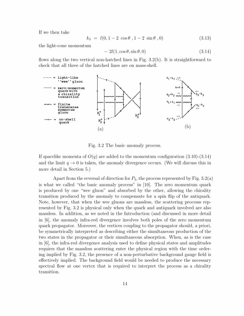
To have all on-shell lines carry the same light-like momentum (around a loop)in a multiple discontinuity is a very restrictive requirement. The essential pointbecomes clear if we consider a physical region double discontinuity which gives thecut lines of Fig. 3.1(a), as in Fig. 3.3(a).

Fig. 3.3 (a) A physical threshold double discontinuity (b) A pseudothreshold doublediscontinuity.

15

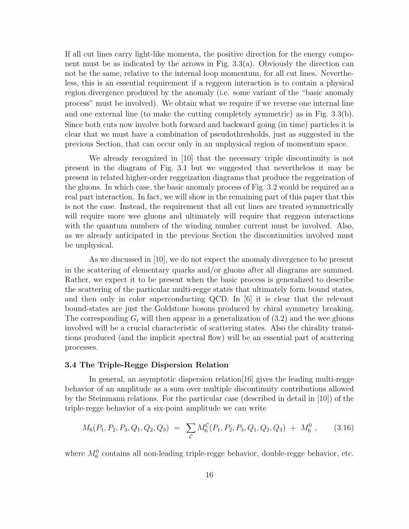
If all cut lines carry light-like momenta, the positive direction for the energy compo-nent must be as indicated by the arrows in Fig. 3.3(a). Obviously the direction cannot be the same, relative to the internal loop momentum, for all cut lines. Neverthe-less, this is an essential requirement if a reggeon interaction is to contain a physicalregion divergence produced by the anomaly (i.e. some variant of the “basic anomaly

process” must be involved). We obtain what we require if we reverse one internal line

and one external line (to make the cutting completely symmetric) as in Fig. 3.3(b).

Since both cuts now involve both forward and backward going (in time) particles it isclear that we must have a combination of pseudothresholds, just as suggested in theprevious Section, that can occur only in an unphysical region of momentum space.

We already recognized in [10] that the necessary triple discontinuity is notpresent in the diagram of Fig. 3.1 but we suggested that nevertheless it may bepresent in related higher-order reggeization diagrams that produce the reggeization ofthe gluons. In which case, the basic anomaly process of Fig. 3.2 would be required as areal part interaction. In fact, we will show in the remaining part of this paper that thisis not the case. Instead, the requirement that all cut lines are treated symmetricallywill require more wee gluons and ultimately will require that reggeon interactionswith the quantum numbers of the winding number current must be involved. Also,as we already anticipated in the previous Section the discontinuities involved mustbe unphysical.

As we discussed in [10], we do not expect the anomaly divergence to be present

in the scattering of elementary quarks and/or gluons after all diagrams are summed.Rather, we expect it to be present when the basic process is generalized to describethe scattering of the particular multi-regge states that ultimately form bound states,and then only in color superconducting QCD. In [6] it is clear that the relevantbound-states are just the Goldstone bosons produced by chiral symmetry breaking.The corresponding Gi will then appear in a generalization of (3.2) and the wee gluonsinvolved will be a crucial characteristic of scattering states. Also the chirality transi-tions produced (and the implicit spectral flow) will be an essential part of scatteringprocesses.

3.4 The Triple-Regge Dispersion Relation

In general, an asymptotic dispersion relation[16] gives the leading multi-reggebehavior of an amplitude as a sum over multiple discontinuity contributions allowedby the Steinmann relations. For the particular case (described in detail in [10]) of thetriple-regge behavior of a six-point amplitude we can write

M6(P1, P2, P3, Q1, Q2, Q3) =∑

C

MC6 (P1, P2, P3, Q1, Q2, Q3) + M0

6 , (3.16)

where M06 contains all non-leading triple-regge behavior, double-regge behavior, etc.

16

and the sum is over all triplets C of asymptotic cuts in non-overlapping (large) in-

variants. For each triplet C, say C = (s1, s2, s3), we can write

MC6 (P1, P2, P3, Q1, Q2, Q3) =

1

(2πi)3

∫

ds′1ds′2ds

′3

∆C

(s′1 − s1)(s′2 − s2)(s′3 − s3)

(3.17)

where ∆C is the triple discontinuity.

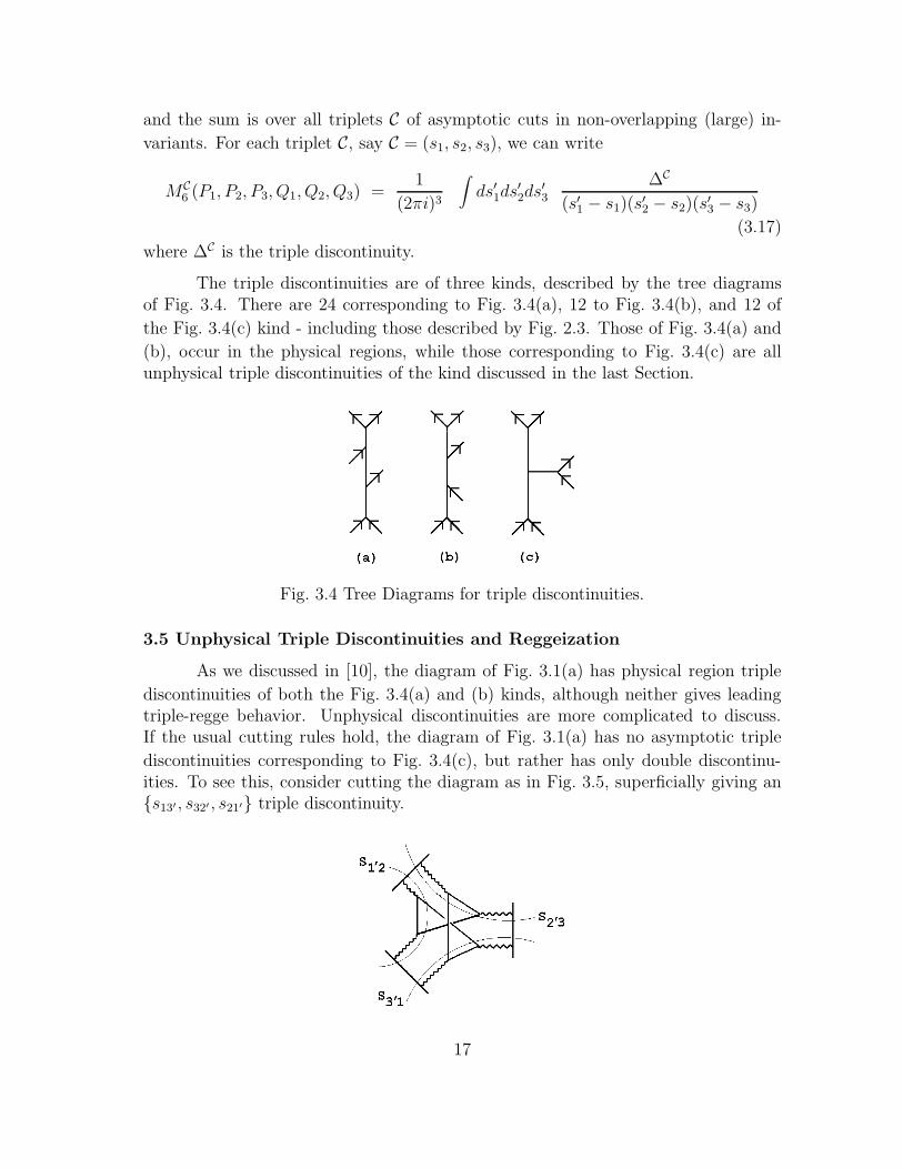
The triple discontinuities are of three kinds, described by the tree diagramsof Fig. 3.4. There are 24 corresponding to Fig. 3.4(a), 12 to Fig. 3.4(b), and 12 of

the Fig. 3.4(c) kind - including those described by Fig. 2.3. Those of Fig. 3.4(a) and

(b), occur in the physical regions, while those corresponding to Fig. 3.4(c) are allunphysical triple discontinuities of the kind discussed in the last Section.

Fig. 3.4 Tree Diagrams for triple discontinuities.

3.5 Unphysical Triple Discontinuities and Reggeization

As we discussed in [10], the diagram of Fig. 3.1(a) has physical region triple

discontinuities of both the Fig. 3.4(a) and (b) kinds, although neither gives leadingtriple-regge behavior. Unphysical discontinuities are more complicated to discuss.If the usual cutting rules hold, the diagram of Fig. 3.1(a) has no asymptotic triple

discontinuities corresponding to Fig. 3.4(c), but rather has only double discontinu-ities. To see this, consider cutting the diagram as in Fig. 3.5, superficially giving an{s13′ , s32′ , s21′} triple discontinuity.

17

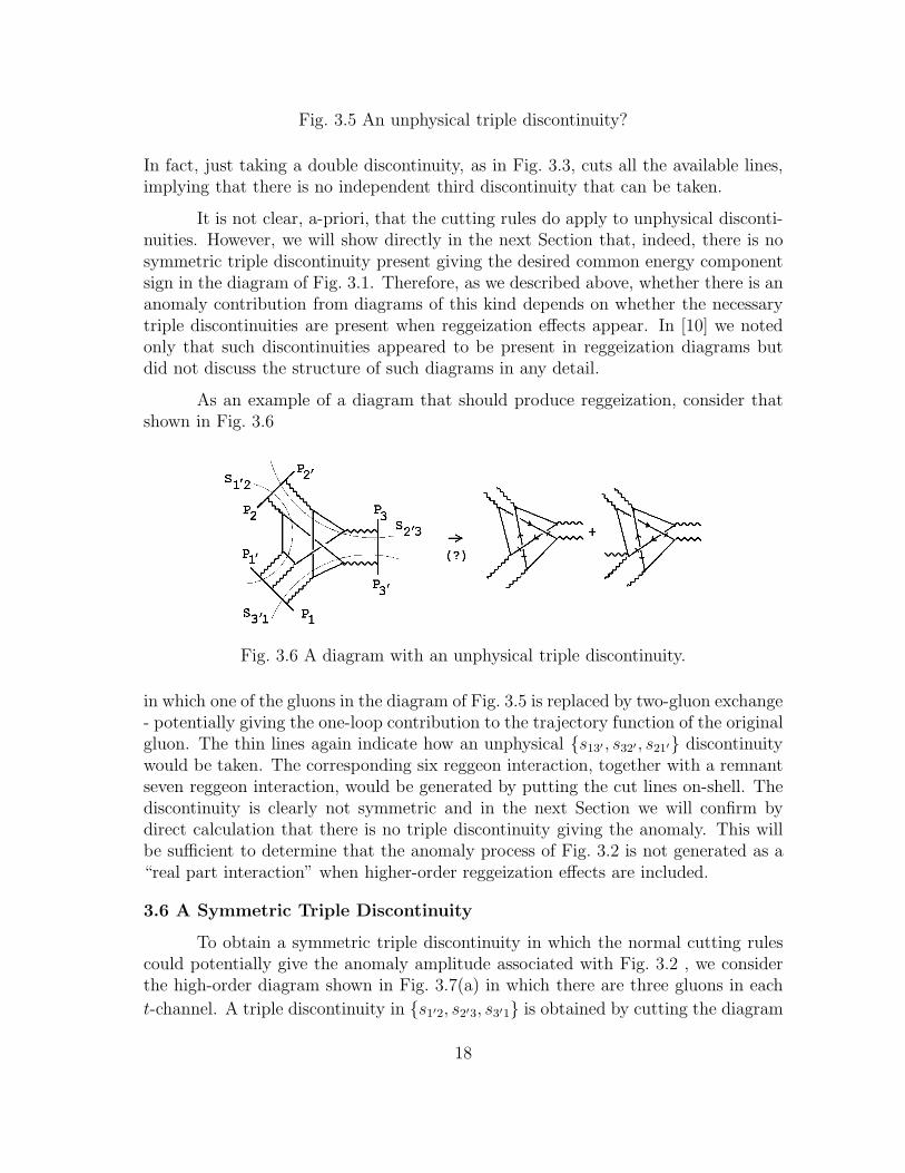
Fig. 3.5 An unphysical triple discontinuity?

In fact, just taking a double discontinuity, as in Fig. 3.3, cuts all the available lines,implying that there is no independent third discontinuity that can be taken.

It is not clear, a-priori, that the cutting rules do apply to unphysical disconti-nuities. However, we will show directly in the next Section that, indeed, there is nosymmetric triple discontinuity present giving the desired common energy componentsign in the diagram of Fig. 3.1. Therefore, as we described above, whether there is ananomaly contribution from diagrams of this kind depends on whether the necessarytriple discontinuities are present when reggeization effects appear. In [10] we notedonly that such discontinuities appeared to be present in reggeization diagrams butdid not discuss the structure of such diagrams in any detail.

As an example of a diagram that should produce reggeization, consider thatshown in Fig. 3.6

Fig. 3.6 A diagram with an unphysical triple discontinuity.

in which one of the gluons in the diagram of Fig. 3.5 is replaced by two-gluon exchange- potentially giving the one-loop contribution to the trajectory function of the originalgluon. The thin lines again indicate how an unphysical {s13′ , s32′, s21′} discontinuitywould be taken. The corresponding six reggeon interaction, together with a remnantseven reggeon interaction, would be generated by putting the cut lines on-shell. Thediscontinuity is clearly not symmetric and in the next Section we will confirm bydirect calculation that there is no triple discontinuity giving the anomaly. This willbe sufficient to determine that the anomaly process of Fig. 3.2 is not generated as a“real part interaction” when higher-order reggeization effects are included.

3.6 A Symmetric Triple Discontinuity

To obtain a symmetric triple discontinuity in which the normal cutting rulescould potentially give the anomaly amplitude associated with Fig. 3.2 , we considerthe high-order diagram shown in Fig. 3.7(a) in which there are three gluons in each

t-channel. A triple discontinuity in {s1′2, s2′3, s3′1} is obtained by cutting the diagram

18

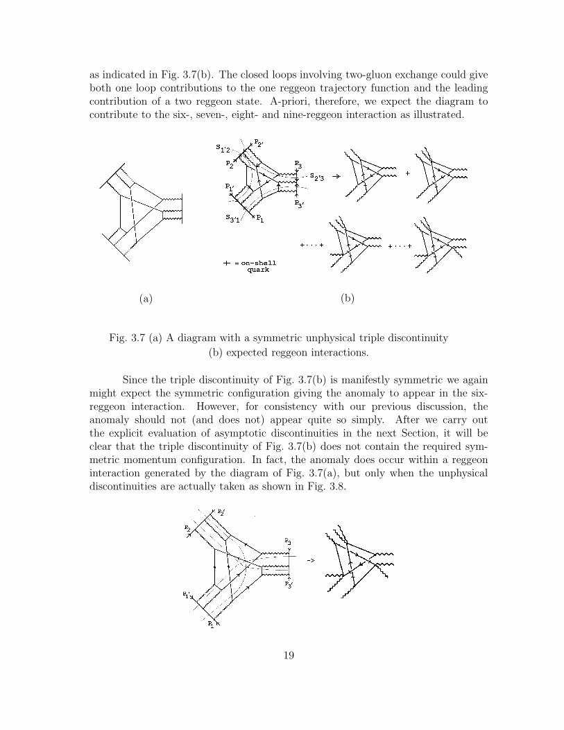
as indicated in Fig. 3.7(b). The closed loops involving two-gluon exchange could giveboth one loop contributions to the one reggeon trajectory function and the leadingcontribution of a two reggeon state. A-priori, therefore, we expect the diagram tocontribute to the six-, seven-, eight- and nine-reggeon interaction as illustrated.

(a) (b)

Fig. 3.7 (a) A diagram with a symmetric unphysical triple discontinuity

(b) expected reggeon interactions.

Since the triple discontinuity of Fig. 3.7(b) is manifestly symmetric we againmight expect the symmetric configuration giving the anomaly to appear in the six-reggeon interaction. However, for consistency with our previous discussion, theanomaly should not (and does not) appear quite so simply. After we carry outthe explicit evaluation of asymptotic discontinuities in the next Section, it will beclear that the triple discontinuity of Fig. 3.7(b) does not contain the required sym-metric momentum configuration. In fact, the anomaly does occur within a reggeoninteraction generated by the diagram of Fig. 3.7(a), but only when the unphysicaldiscontinuities are actually taken as shown in Fig. 3.8.

19

Fig. 3.8 Another cutting of Fig. 3.7(a).

However, we will postpone until Section 5 a discussion of which reggeon interactionis involved. Note that the discontinuity lines in Fig. 3.8 cross each other. We willsee that this is possible because, as anticipated in the previous Section, the particlescontributing to each discontinuity will not all have the same time direction. Toevaluate a multiple discontinuity of this kind we must develop direct methods tocompute asymptotic discontinuities.

20

4. UNPHYSICAL TRIPLE DISCONTINUITIES AND

HIGHER-ORDER GRAPHS

In this Section we generalize the single asymptotic discontinuity analysis de-scribed in the Appendix to asymptotic triple discontinuities. The essential idea is thatthere is a well-defined leading-log result for each triple discontinuity (just as there is

for the single discontinuity calculated in the Appendix) that can be found from theleading-log calculation of amplitudes by keeping the iǫ dependence of all logarithms.

4.1 A Physical Region Discontinuity

We begin by considering again the maximally non-planar graph shown inFig. 3.1. To understand how asymptotic discontinuities arise, we first consider a phys-ical region discontinuity. For this we interchange P1 and P1′ in (3.1) so that P1′ and P2

are the momenta of incoming particles. For simplicity, we also set Qi = 0, i = 1, 2, 3.This could cause confusion as to which invariants discontinuities actually occur in.However, for the discontinuities that interest us, we will be able to avoid this issue.(As is the case for our discussion in the Appendix, adding both transverse momentaand masses to our discussion would not change the essential features of the analysis,but would eliminate gluon infra-red divergences. We will discuss, at some points, thegeneral effect of adding transverse momenta.) Therefore we write, asymptotically,

P1′ → − P1 = (p1′ , p1′, 0, 0) , p1′ → ∞P2 → − P2′ = (p2, 0, p2, 0) , p2 → ∞P3 → − P3′ = (p3, 0, 0, p3) , p3 → ∞

(4.1)

For the reasons given in the last Section, we will ultimately be looking for asymmetric triple discontinuity. Therefore, we consider only routes for the internalloop momenta of Fig. 3.1 that are completely symmetric with respect to the threeexternal loops. There is essentially only one possibility. The two apparently distinctpossibilities illustrated in Fig. 4.1 are related by interchanging the primed and un-primed external momenta. We will also want to make a symmetric choice for thequark lines we place on shell. Although we will not discuss the anomaly in detailuntil the next Section, in anticipation of this we will demand that a product of threeorthogonal γ-matrices be associated with the process of putting on-shell each internalquark line. To achieve this it is necessary to put on-shell, symmetrically, the internallines in Fig. 4.1(a) along which a single loop momentum flows. Therefore, we consideronly such lines in the following.

21

(a) (b)

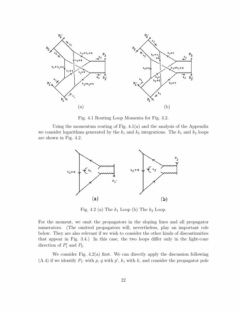
Fig. 4.1 Routing Loop Momenta for Fig. 3.2.

Using the momentum routing of Fig. 4.1(a) and the analysis of the Appendixwe consider logarithms generated by the k1 and k2 integrations. The k1 and k2 loopsare shown in Fig. 4.2.

Fig. 4.2 (a) The k1 Loop (b) The k2 Loop.

For the moment, we omit the propagators in the sloping lines and all propagatornumerators. (The omitted propagators will, nevertheless, play an important rolebelow. They are also relevant if we wish to consider the other kinds of discontinuitiesthat appear in Fig. 3.4.) In this case, the two loops differ only in the light-cone

direction of P ′1 and P2.

We consider Fig. 4.2(a) first. We can directly apply the discussion following

(A.4) if we identify P1′ with p, q with p′, k1 with k, and consider the propagator pole

22

at (k1 + q)2 = 0. We then obtain

I(p1′q1−) ∼ i∫

d2k1⊥[

−k21⊥ + iǫ]−2

∫ λq1−

0dk1− [k1− − q1− ]

−1[

p1′k1− − k21⊥ + iǫ]−1

∼ 1

p1′q1−log [p1′λq1− + iǫ]

(4.2)

We have used the notation (used extensively in the following) that for any four-momentum k

ki± = k0 ± ki ki⊥ = (kj, kk) j 6= k 6= i i, j, k = 1, 2, 3 (4.3)

The q1− dependence indicates that the logarithm is a reflection of a threshold in theinvariant P1′ ·q . This dependence plays an important role in the following discussion.We also retain the λ-dependence, for technical reasons that will become apparentlater. The final result will be independent of λ, as it must be. From Fig. 4.2(b) weanalagously obtain

I(p2q2−) ∼ 1

p2q2−log [−p2λq2− + iǫ] (4.4)

The minus sign (which is very important in the following) appears relative to (4.2)because of the opposite direction of P2.

Next we consider how the logarithmic branch cuts generated by the k1 andk2 integrations can trap the internal loop integration over q to produce an overalldiscontinuity in s1′2 ∼ p1′p2. For simplicity, we consider the region where

k2i⊥ ∼ q2 ∼ 0 i = 1, 2, 3 (4.5)

Appealing to (A.6) we can then, for our present purposes, effectively ignore the re-

maining ki dependence of the quark loop (including the propagators that we ignored

in the above discussion). If we parameterize q as

q =(

q0, q1−, q2−, q3−)

(4.6)

we can treat the qi− as independent variables, with q0 essentially determined by the

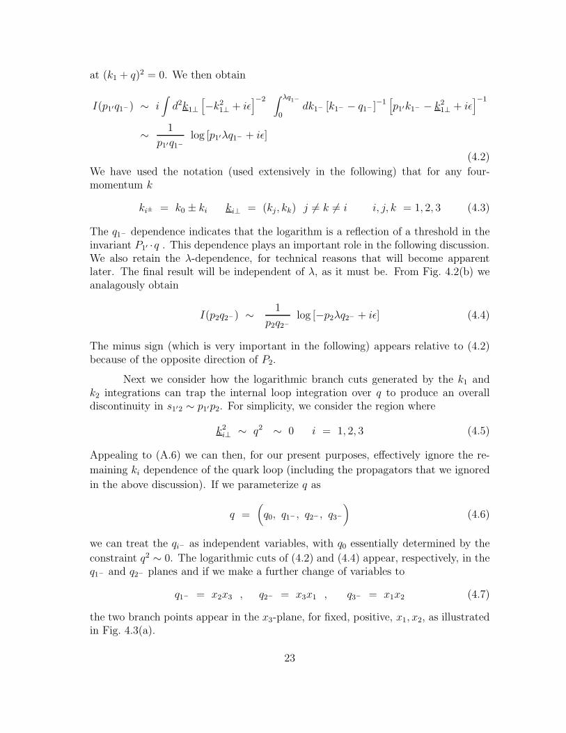
constraint q2 ∼ 0. The logarithmic cuts of (4.2) and (4.4) appear, respectively, in theq1− and q2− planes and if we make a further change of variables to

q1− = x2x3 , q2− = x3x1 , q3− = x1x2 (4.7)

the two branch points appear in the x3-plane, for fixed, positive, x1, x2, as illustratedin Fig. 4.3(a).

23

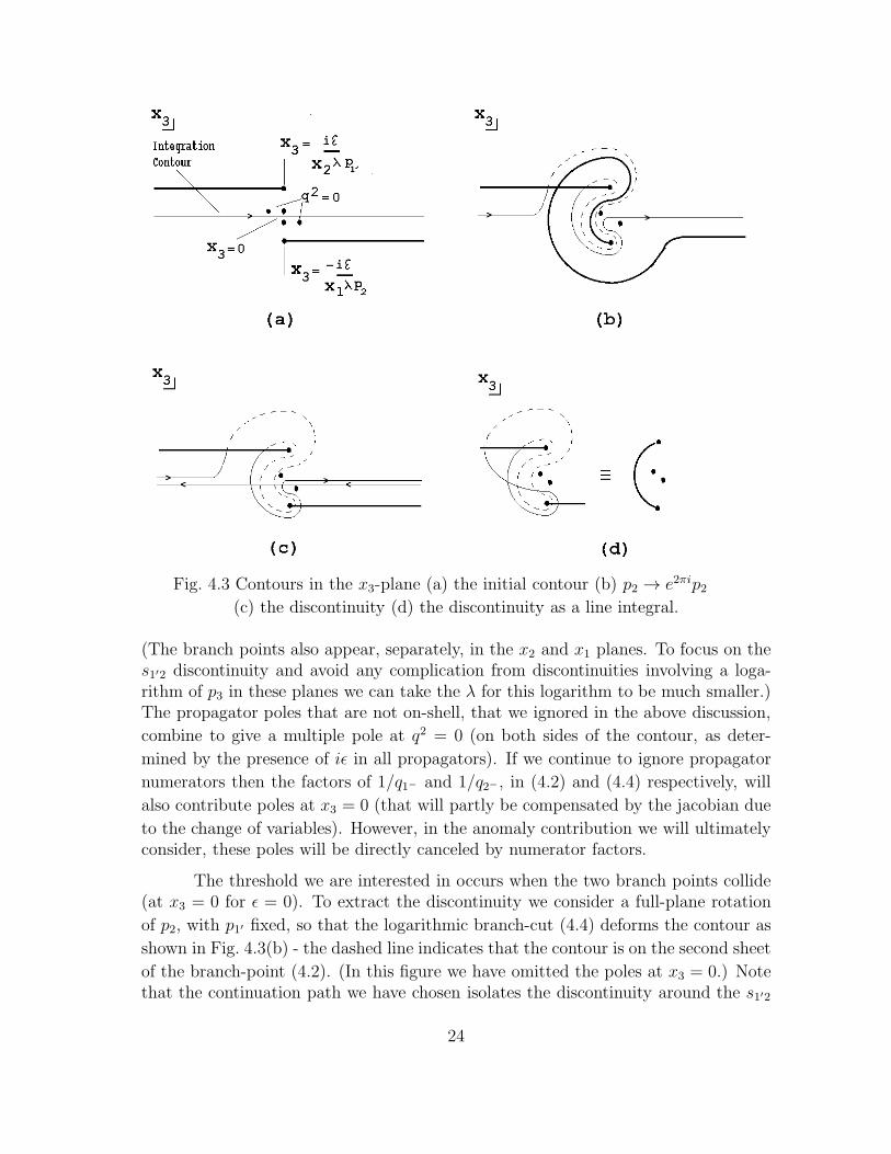
Fig. 4.3 Contours in the x3-plane (a) the initial contour (b) p2 → e2πip2(c) the discontinuity (d) the discontinuity as a line integral.

(The branch points also appear, separately, in the x2 and x1 planes. To focus on thes1′2 discontinuity and avoid any complication from discontinuities involving a loga-rithm of p3 in these planes we can take the λ for this logarithm to be much smaller.)The propagator poles that are not on-shell, that we ignored in the above discussion,

combine to give a multiple pole at q2 = 0 (on both sides of the contour, as deter-

mined by the presence of iǫ in all propagators). If we continue to ignore propagator

numerators then the factors of 1/q1− and 1/q2−, in (4.2) and (4.4) respectively, will

also contribute poles at x3 = 0 (that will partly be compensated by the jacobian due

to the change of variables). However, in the anomaly contribution we will ultimatelyconsider, these poles will be directly canceled by numerator factors.

The threshold we are interested in occurs when the two branch points collide(at x3 = 0 for ǫ = 0). To extract the discontinuity we consider a full-plane rotation

of p2, with p1′ fixed, so that the logarithmic branch-cut (4.4) deforms the contour as

shown in Fig. 4.3(b) - the dashed line indicates that the contour is on the second sheet

of the branch-point (4.2). (In this figure we have omitted the poles at x3 = 0.) Notethat the continuation path we have chosen isolates the discontinuity around the s1′2

24

branch cut, since it avoids the pinching of the integration contour with the singularity

at q2 = 0 that would give other discontinuities. The desired discontinuity is obtainedby adding the original contour in the opposite direction, as shown in Fig. 4.3(c).

Combining both contours we obtain Fig. 4.3(d) which, as illustrated, can be writtenas a line integral between the two branch points of the double-discontinuity due toboth cuts. As ǫ → 0, or in the asymptotic limit p1′, p2 → ∞, the branch pointsapproach each other and the result is a closed contour integral around the singularity

at q2 = 0 which is independent of the position of the end points and remains finitein the asymptotic limit. This is the asymptotic discontinuity and the singularity at

q2 = 0 is clearly crucial in producing a non-zero result.

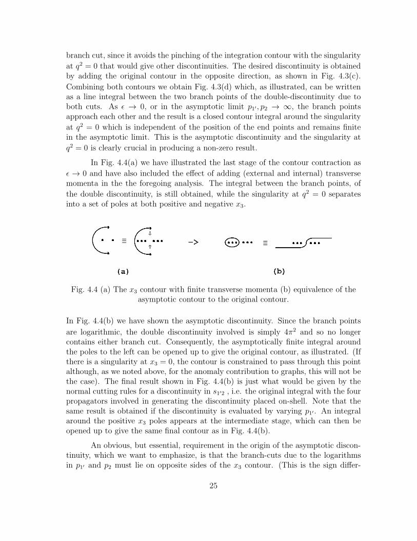
In Fig. 4.4(a) we have illustrated the last stage of the contour contraction as

ǫ → 0 and have also included the effect of adding (external and internal) transversemomenta in the the foregoing analysis. The integral between the branch points, of

the double discontinuity, is still obtained, while the singularity at q2 = 0 separatesinto a set of poles at both positive and negative x3.

Fig. 4.4 (a) The x3 contour with finite transverse momenta (b) equivalence of theasymptotic contour to the original contour.

In Fig. 4.4(b) we have shown the asymptotic discontinuity. Since the branch points

are logarithmic, the double discontinuity involved is simply 4π2 and so no longercontains either branch cut. Consequently, the asymptotically finite integral aroundthe poles to the left can be opened up to give the original contour, as illustrated. (Ifthere is a singularity at x3 = 0, the contour is constrained to pass through this pointalthough, as we noted above, for the anomaly contribution to graphs, this will not bethe case). The final result shown in Fig. 4.4(b) is just what would be given by thenormal cutting rules for a discontinuity in s1′2 , i.e. the original integral with the fourpropagators involved in generating the discontinuity placed on-shell. Note that thesame result is obtained if the discontinuity is evaluated by varying p1′. An integralaround the positive x3 poles appears at the intermediate stage, which can then beopened up to give the same final contour as in Fig. 4.4(b).

An obvious, but essential, requirement in the origin of the asymptotic discon-tinuity, which we want to emphasize, is that the branch-cuts due to the logarithmsin p1′ and p2 must lie on opposite sides of the x3 contour. (This is the sign differ-

25

ence between (4.2) and (4.4) that we emphasized above.) In a physical region thisrequirement is normally straightforward for a loop integration producing a thresholddue to two massive states since the loop momentum will flow oppositely through thetwo states and the iǫ prescription will place the states on opposite sides of the energyintegration contour. In the variables we are using the generation of the thresholdis a little more subtle. Note, for example, that when x1 < 0 the branch-point (4.2)

appears in the upper half-plane (moving through infinity as x1 moves through zero)and there is no discontinuity. Therefore, the signs of the xi play an essential rolein the occurrence of the discontinuity. A further requirement, which clearly holds inthe case just discussed, is that the trapping (pinching) of the contour that we havediscussed must combine with the pinching associated with the logarithms to give acomplete cut through the diagram. That is to say, the complete set of pinchings mustcorrespond to an overall invariant cut.

4.2 Maximally Non-Planar Unphysical Discontinuities

We consider next the unphysical discontinuities that are our principal interest.According to the discussion in Section 3, we are looking for a triple discontinuity ofthe form of Fig. 3.5 that treats the three cut lines of the quark loop symmetricallyso that, in a physical region, the sign of the energy component can be the same forall three on-shell states. We will, therefore, confine our discussion to a search for asymmetric triple discontinuity. As we noted, if the normal cutting rules apply there isno triple discontinuity (symmetric or not) of the Fig. 3.5 kind. We consider whetherthe direct evaluation of discontinuities gives the same result.

The discontinuity we discussed above occurred in a physical region that isunsymmetric in that P2 is the momentum of an incoming particle while P1 is themomentum of an outgoing particle. To look for a symmetric discontinuity we will usean analysis that treats the complete graph symmetrically throughout. To this end,we start in the symmetric asymptotic region (3.1) where all momenta are real and

si′j ∼ − pipj < 0 (4.8)

In this region, the diagram is defined by the usual iǫ prescription. Since all threeinvariants must be positive, the triple discontinuity of Fig. 3.5 can only be presentin the triple-regge limit if we allow the large momenta involved to be unphysical. Asymmetric way to do this is to start from the real physical region and take

pi → e−iπ/2pi = ipi , i = 1, 2, 3 => si′j ∼ (−ipi)(ipj) > 0 (4.9)

Given the symmetry of the present discussion, it is immediately apparent thatthere will not be a (symmetric) triple discontinuity, as we now argue. Using the aboveanalysis, logarithms will be generated by each of the ki integrations. If we consideragain the region where the transverse momenta are close to zero then, from (A.6),

26

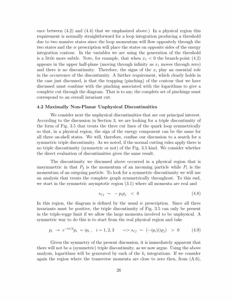
the requirement that the energy component of each on-shell line in the loop have thesame sign is equivalent to requiring that the qi− all have the same sign. This, in turn,requires that the xi should all have the same sign. However, in the symmetric realphysical region, if x1 and x2 have the same sign, the logarithmic branch cuts in P1

and P2 lie on the same side of the x3 contour as illustrated in Fig. 4.5.

Fig. 4.5 The Symmetric Location of Branch-Cuts in the x3-plane.

Since the continuation (4.9) is symmetric they will remain on the same side afterthe continuation. As a consequence, in the symmetric xi region, the contour will notbe trapped and distorted as one branch point moves aound the other, as it was inFig. 4.3, and no discontinuity will result. We conclude therefore that, for the graphwe are discussing, discontinuities can only be generated in asymmetric regions of thexi that can not provide the symmetric triple discontinuity that we are looking for.The foregoing analysis also precludes the occurence of a triple discontinuity, that isappropriately symmetric, in the diagram of Fig. 3.6.

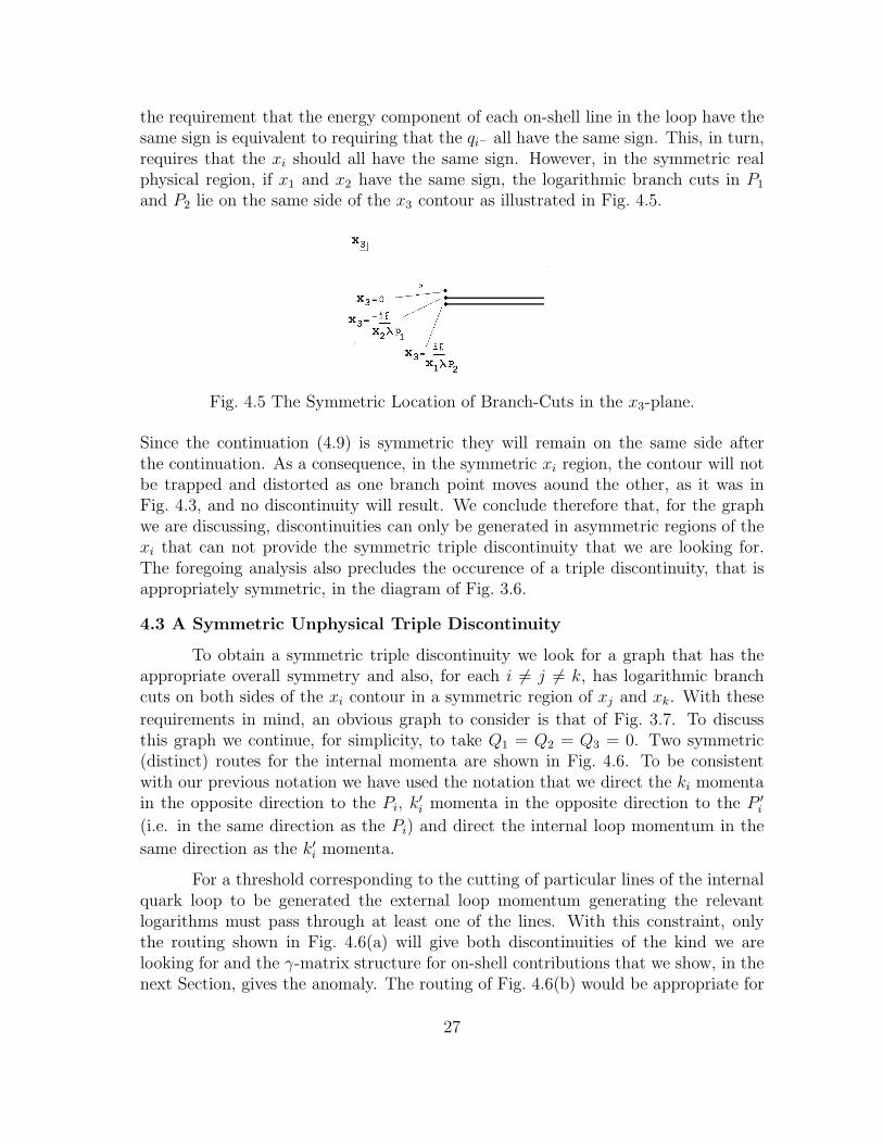
4.3 A Symmetric Unphysical Triple Discontinuity

To obtain a symmetric triple discontinuity we look for a graph that has theappropriate overall symmetry and also, for each i 6= j 6= k, has logarithmic branchcuts on both sides of the xi contour in a symmetric region of xj and xk. With these

requirements in mind, an obvious graph to consider is that of Fig. 3.7. To discussthis graph we continue, for simplicity, to take Q1 = Q2 = Q3 = 0. Two symmetric(distinct) routes for the internal momenta are shown in Fig. 4.6. To be consistentwith our previous notation we have used the notation that we direct the ki momentain the opposite direction to the Pi, k

′i momenta in the opposite direction to the P ′

i

(i.e. in the same direction as the Pi) and direct the internal loop momentum in the

same direction as the k′i momenta.

For a threshold corresponding to the cutting of particular lines of the internalquark loop to be generated the external loop momentum generating the relevantlogarithms must pass through at least one of the lines. With this constraint, onlythe routing shown in Fig. 4.6(a) will give both discontinuities of the kind we arelooking for and the γ-matrix structure for on-shell contributions that we show, in thenext Section, gives the anomaly. The routing of Fig. 4.6(b) would be appropriate for

27

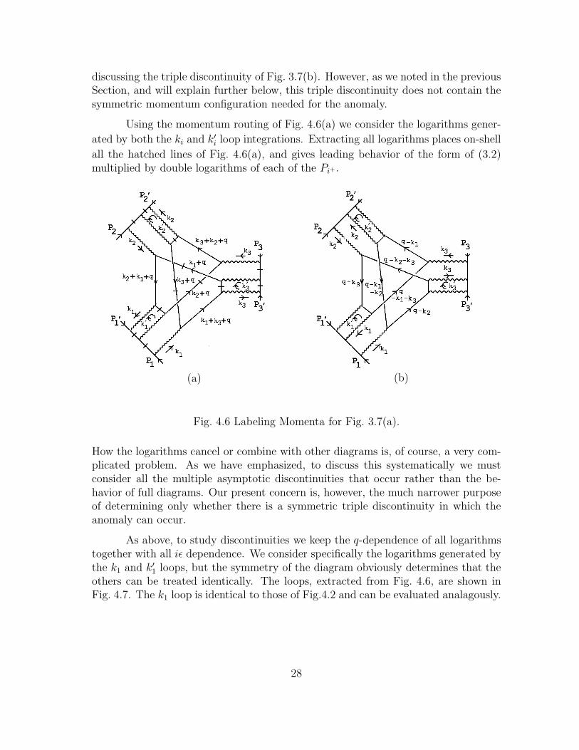
discussing the triple discontinuity of Fig. 3.7(b). However, as we noted in the previousSection, and will explain further below, this triple discontinuity does not contain thesymmetric momentum configuration needed for the anomaly.

Using the momentum routing of Fig. 4.6(a) we consider the logarithms gener-

ated by both the ki and k′i loop integrations. Extracting all logarithms places on-shell

all the hatched lines of Fig. 4.6(a), and gives leading behavior of the form of (3.2)multiplied by double logarithms of each of the Pi+.

(a) (b)

Fig. 4.6 Labeling Momenta for Fig. 3.7(a).

How the logarithms cancel or combine with other diagrams is, of course, a very com-plicated problem. As we have emphasized, to discuss this systematically we mustconsider all the multiple asymptotic discontinuities that occur rather than the be-havior of full diagrams. Our present concern is, however, the much narrower purposeof determining only whether there is a symmetric triple discontinuity in which theanomaly can occur.

As above, to study discontinuities we keep the q-dependence of all logarithmstogether with all iǫ dependence. We consider specifically the logarithms generated bythe k1 and k

′1 loops, but the symmetry of the diagram obviously determines that the

others can be treated identically. The loops, extracted from Fig. 4.6, are shown inFig. 4.7. The k1 loop is identical to those of Fig.4.2 and can be evaluated analagously.

28

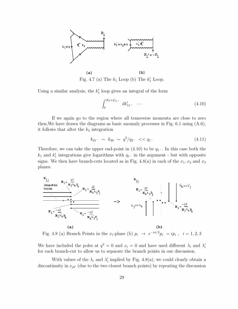
Fig. 4.7 (a) The k1 Loop (b) The k′1 Loop.

Using a similar analysis, the k′1 loop gives an integral of the form

∫ (k2+q)1−

0dk′11− · · · (4.10)

If we again go to the region where all transverse momenta are close to zerothen,We have drawn the diagrams as basic anomaly processes in Fig. 6.1 using (A.6),it follows that after the k2 integration

k21− ∼ k20 ∼ q2/q2− << q1− (4.11)

Therefore, we can take the upper end-point in (4.10) to be q1− . In this case both the

k1 and k′1 integrations give logarithms with q1− in the argument - but with opposite

signs. We then have branch-cuts located as in Fig. 4.8(a) in each of the x1, x2 and x3planes.

Fig. 4.8 (a) Branch Points in the xi-plane (b) pi → e−iπ/2pi = ipi , i = 1, 2, 3

We have included the poles at q2 = 0 and xi = 0 and have used different λi and λ′i

for each branch-cut to allow us to separate the branch points in our discussion.

With values of the λi and λ′i implied by Fig. 4.8(a), we could clearly obtain a

discontinuity in sjk′ (due to the two closest branch points) by repeating the discussion

29

illustrated by Fig. 4.3. The discontinuity would similarly be an integral between thetwo branch points involved, as in Fig. 4.3(d), but because of the additional branchpoints that are present, the contour could not be opened up as in Fig. 4.4. Therefore,having taken xj , xk > 0 so that the branch cuts lie as in Fig. 4.8(a), the discontinuity

would involve only pure imaginary or negative real part values of xi. Consequently,any further discontinuity obtained by the collision of branch points in the xj or xkplanes would have to involve mixed real part signs for the xi. We conclude (not

surprisingly) that in the physical region a triple discontinuity can not be obtainedthat involves only positive values of all three xi.

This brings us to the central point of the paper. If we go to the unphysicalregion (4.9), where we expect to encounter an unphysical triple discontinuity, the lastanalysis changes in a crucial manner. The resulting location of branch cuts is nowas shown in Fig. 4.8(b), allowing the integration contour to be rotated as illustrated.

In Fig. 4.8(b) we have also, for emphasis, chosen significantly different values of the

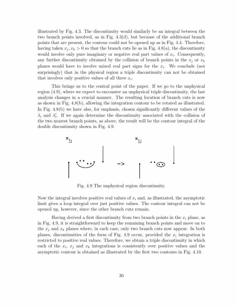
λi and λ′i. If we again determine the discontinuity associated with the collision ofthe two nearest branch points, as above, the result will be the contour integral of thedouble discontinuity shown in Fig. 4.9.

Fig. 4.9 The unphysical region discontinuity.

Now the integral involves positive real values of xi and, as illustrated, the asymptoticlimit gives a loop integral over just positive values. The contour integral can not beopened up, however, since the other branch cuts remain.

Having derived a first discontinuity from two branch points in the xi plane, asin Fig. 4.9, it is straightforward to keep the remaining branch points and move on tothe xj and xk planes where, in each case, only two branch cuts now appear. In both

planes, discontinuities of the form of Fig. 4.9 occur, provided the xi integration isrestricted to positive real values. Therefore, we obtain a triple discontinuity in whicheach of the xi, xj and xk integrations is consistently over positive values and the

asymptotic contour is obtained as illustrated by the first two contours in Fig. 4.10.

30

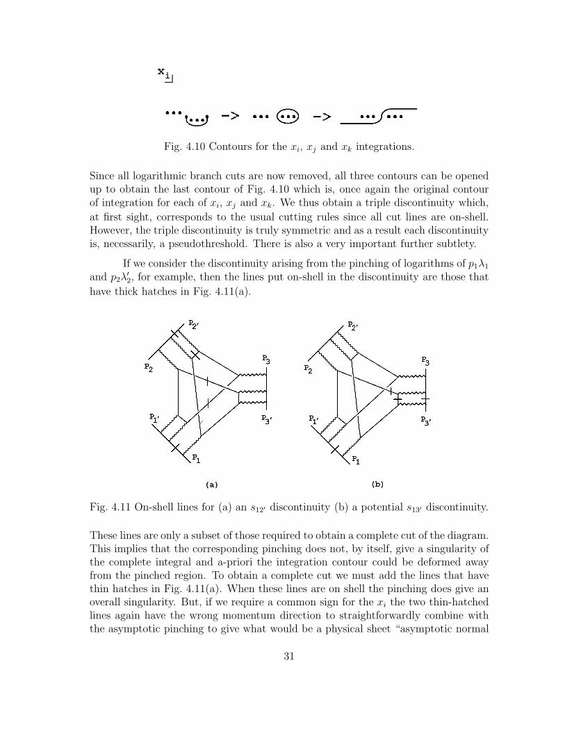
Fig. 4.10 Contours for the xi, xj and xk integrations.

Since all logarithmic branch cuts are now removed, all three contours can be openedup to obtain the last contour of Fig. 4.10 which is, once again the original contourof integration for each of xi, xj and xk. We thus obtain a triple discontinuity which,

at first sight, corresponds to the usual cutting rules since all cut lines are on-shell.However, the triple discontinuity is truly symmetric and as a result each discontinuityis, necessarily, a pseudothreshold. There is also a very important further subtlety.

If we consider the discontinuity arising from the pinching of logarithms of p1λ1and p2λ

′2, for example, then the lines put on-shell in the discontinuity are those that

have thick hatches in Fig. 4.11(a).

Fig. 4.11 On-shell lines for (a) an s12′ discontinuity (b) a potential s13′ discontinuity.

These lines are only a subset of those required to obtain a complete cut of the diagram.This implies that the corresponding pinching does not, by itself, give a singularity ofthe complete integral and a-priori the integration contour could be deformed awayfrom the pinched region. To obtain a complete cut we must add the lines that havethin hatches in Fig. 4.11(a). When these lines are on shell the pinching does give anoverall singularity. But, if we require a common sign for the xi the two thin-hatchedlines again have the wrong momentum direction to straightforwardly combine withthe asymptotic pinching to give what would be a physical sheet “asymptotic normal

31

threshold”. However, each of the two thin hatched lines is separately placed on shellby one of the additional discontinuities. Therefore, the full triple discontinuity wehave found does correspond to a triplet {s12′ , s23′ , s32′} of invariant (pseudothreshold)cuts.

If we consider instead the discontinuity arising from the pinching of logarithmsof p1λ1 and p3λ

′3 then the lines put on shell are those hatched in Fig. 4.11(b). In this

case there is no simple way to include additional lines and obtain an invariant cut.Therefore, this pinching can not be extended to a complete cut of the diagram. Weconclude that the triple discontinuity in {s12′ , s23′ , s32′} that is illustrated in Fig. 3.8is the only combination that exists, as an extension of the above analysis. It is sym-metric, with each of the internal quark lines that are put on shell by ki integrationstreated symmetrically. All three of these lines contribute to each invariant cut but,as we have just discussed, two of them always have the wrong iǫ prescription, rela-tive to the third, to give a physical normal threshold. Singularities associated withcombinations of forward and backward going particles are “mixed-α” solutions of theLandau equations[16]. In general, such “pseudothresholds” are not singular on thephysical sheet because of the conflicting iǫ prescriptions. However, they are generallysingular on unphysical sheets and can appear in multiple discontinuities. They wouldbe particularly expected to appear in unphysical multiple discontinuities.

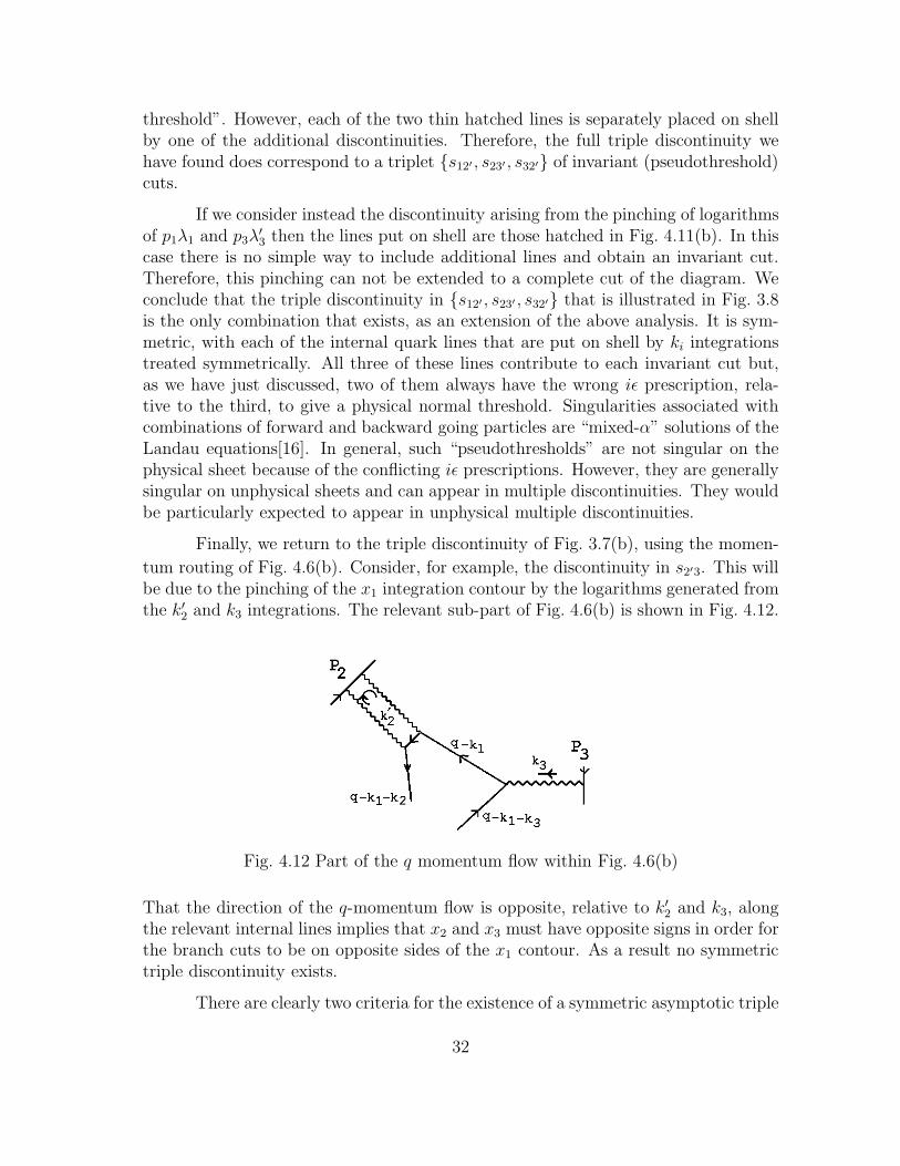
Finally, we return to the triple discontinuity of Fig. 3.7(b), using the momen-

tum routing of Fig. 4.6(b). Consider, for example, the discontinuity in s2′3. This willbe due to the pinching of the x1 integration contour by the logarithms generated fromthe k′2 and k3 integrations. The relevant sub-part of Fig. 4.6(b) is shown in Fig. 4.12.

Fig. 4.12 Part of the q momentum flow within Fig. 4.6(b)

That the direction of the q-momentum flow is opposite, relative to k′2 and k3, alongthe relevant internal lines implies that x2 and x3 must have opposite signs in order forthe branch cuts to be on opposite sides of the x1 contour. As a result no symmetrictriple discontinuity exists.

There are clearly two criteria for the existence of a symmetric asymptotic triple

32

discontinuity - that we will appeal to further in the next Section. The first is that theq momentum flow must be in the same relative direction along the relevant internallines for each discontinuity. The second is that all internal loop lines, besides those inthe remaining triangle, must be put on shell by the combination of the three pinchesof the xi integrations.

33

5. THE TRIANGLE ANOMALY AND OTHER

DIAGRAMS

In this Section we discuss how the anomaly occurs in a reggeon vertex obtainedfrom the triple discontinuity of Fig. 3.8. We will also consider other diagrams thatcan contribute and discuss how color quantum numbers determine which reggeoninteractions are involved.

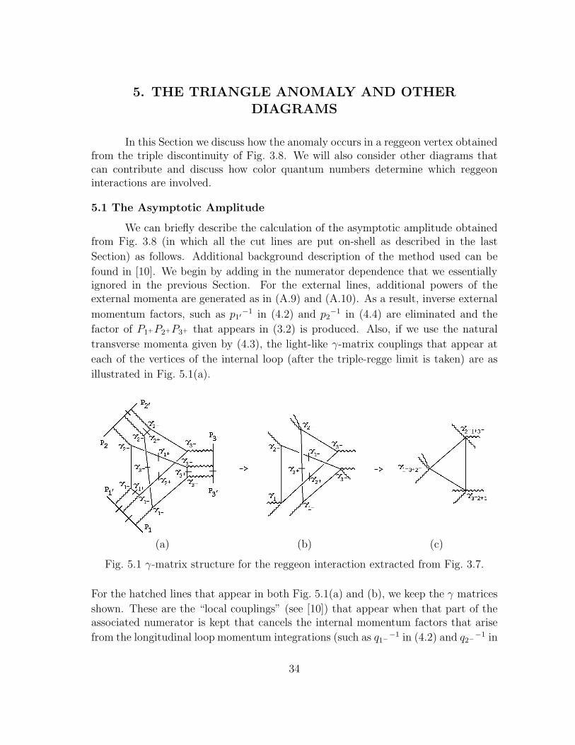
5.1 The Asymptotic Amplitude

We can briefly describe the calculation of the asymptotic amplitude obtainedfrom Fig. 3.8 (in which all the cut lines are put on-shell as described in the last

Section) as follows. Additional background description of the method used can be

found in [10]. We begin by adding in the numerator dependence that we essentiallyignored in the previous Section. For the external lines, additional powers of theexternal momenta are generated as in (A.9) and (A.10). As a result, inverse external

momentum factors, such as p1′−1 in (4.2) and p2

−1 in (4.4) are eliminated and the

factor of P1+P2+P3+ that appears in (3.2) is produced. Also, if we use the natural

transverse momenta given by (4.3), the light-like γ-matrix couplings that appear at

each of the vertices of the internal loop (after the triple-regge limit is taken) are as

illustrated in Fig. 5.1(a).

(a) (b) (c)

Fig. 5.1 γ-matrix structure for the reggeon interaction extracted from Fig. 3.7.

For the hatched lines that appear in both Fig. 5.1(a) and (b), we keep the γ matrices

shown. These are the “local couplings” (see [10]) that appear when that part of theassociated numerator is kept that cancels the internal momentum factors that arise

from the longitudinal loop momentum integrations (such as q1−−1 in (4.2) and q2−

−1 in

34

(4.4) ). To justify this procedure we appeal to the (“infra-red non-renormalization”)

argument of Coleman and Grossman[17] that only a fermion triangle diagram, withparticular helicities for the couplings, can produce the anomaly infra-red divergence.

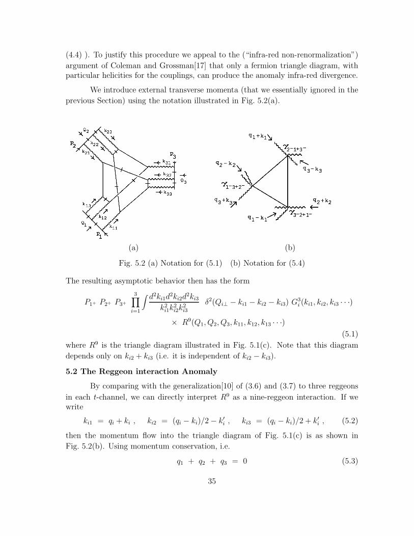
We introduce external transverse momenta (that we essentially ignored in the

previous Section) using the notation illustrated in Fig. 5.2(a).

(a) (b)

Fig. 5.2 (a) Notation for (5.1) (b) Notation for (5.4)

The resulting asymptotic behavior then has the form

P1+ P2+ P3+

3∏

i=1

∫

d2ki1d2ki2d

2ki3k2i1k

2i2k

2i3

δ2(Qi⊥ − ki1 − ki2 − ki3) G3i (ki1, ki2, ki3 · · ·)

× R9(Q1, Q2, Q3, k11, k12, k13 · · ·)(5.1)

where R9 is the triangle diagram illustrated in Fig. 5.1(c). Note that this diagram

depends only on ki2 + ki3 (i.e. it is independent of ki2 − ki3).

5.2 The Reggeon interaction Anomaly

By comparing with the generalization[10] of (3.6) and (3.7) to three reggeons

in each t-channel, we can directly interpret R9 as a nine-reggeon interaction. If wewrite

ki1 = qi + ki , ki2 = (qi − ki)/2− k′i , ki3 = (qi − ki)/2 + k′i , (5.2)

then the momentum flow into the triangle diagram of Fig. 5.1(c) is as shown in

Fig. 5.2(b). Using momentum conservation, i.e.

q1 + q2 + q3 = 0 (5.3)

35

R9, which does not depend on the k′i, can be written (very similarly to (3.4)) as

R9(q1, q2, q3, k1, k2, k3) =∫

d4kTr{γ5γ1−3+2−(k/ + k/2 + q/3 − k/1)

γ5γ2−1+3−(k/ − q/2 + q/3 − k/2 − k/3)γ5γ

3−2+1−(k/ + k/1 − q/2 − k/3)}(k + k2 + q3 − k1)2(k − q2 + q3 − k2 − k3)2(k + k1 − q2 − k3)2

(5.4)

where

γ1−3+2− = γ1−γ3+γ2− = γ−,−,− − i γ−,−,+ γ5

γ2−1+3− = γ2−γ1+γ3− = γ−,−,− − i γ+,−,− γ5

γ3−2+1− = γ3−γ2+γ1− = γ−,−,− − i γ−,+,− γ5

(5.5)

and γ±,±,± is defined by (3.5). Again we obtain a particular component of the tensorthat describes the triangle diagram contribution to a three current vertex function,i.e. we can write

R9(q1, q2, q3, k1, k2, k3) = (n−,−,−µ − i n−,−,+

µ )(n−,−,−α − i n+,−,−

α )(n−,−,−β − i n−,+,−

β )

× T µαβ(k1 − k3 − q2, k2 − k1 −−q3)(5.6)

where T µαβ is the triangle diagram three current amplitude.

To discuss the occurence of the anomaly in (5.5) we first recall the general

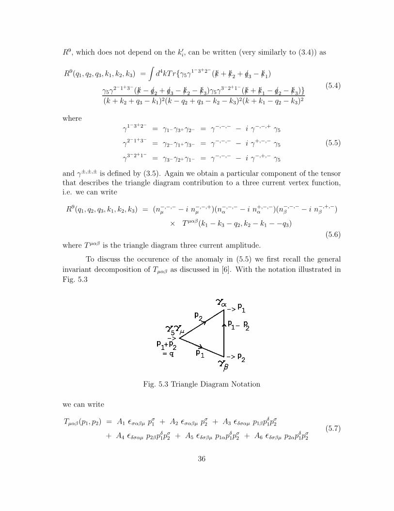
invariant decomposition of Tµαβ as discussed in [6]. With the notation illustrated in

Fig. 5.3

Fig. 5.3 Triangle Diagram Notation

we can write

Tµαβ(p1, p2) = A1 ǫσαβµ pσ1 + A2 ǫσαβµ pσ2 + A3 ǫδσαµ p1βpδ1pσ2

+ A4 ǫδσαµ p2βpδ1pσ2 + A5 ǫδσβµ p1αpδ1p

σ2 + A6 ǫδσβµ p2αpδ1p

σ2

(5.7)

36

The ultra-violet anomaly occurs in the first two terms of (5.7), i.e.

Tµαβ(k1, k2) =1

4π2ǫσαβµ pσ1 +

1

4π2ǫσαβµ pσ2 + · · · (5.8)

leading to the well-known divergence equation

(p1 + p2)µ Tµαβ =

1

2π2ǫδσαβ pδ1pσ2 (5.9)

The ultra-violet anomaly can therefore appear only in a tensor component with threeorthogonal Lorentz indices. If we keep just the γ5 parts of the three vertices in (5.5)we obtain a non-zero projection on such a tensor component. In fact this contribution

to R9 retains the full symmetry of the original feynman diagram of Fig. 3.7(a) and,as a result, has the necessary symmetry to contain the ultra-violet anomaly.

The infra-red “anomaly pole” occurs in A3 and A6. When p21 = 0

A3 = −A6 =1

2π2

1

p22 − q2

(

p22p22 − q2

lnp22q2

− 1)

(5.10)

and when p22 → 0

A3 → 1

2π2

1

q2(5.11)

That is, a pole appears in A3 (= −A6) and, as a consequence of all divergenceequations, the coefficient is also given by the anomaly. If, instead, we integrate over

spacelike values of q2, we obtain

∫

dq2 A3(q2, p22) f(q

2, p22) −→k22 → 0

1

πf(0, 0) =

∫

dq21

πδ(q2) f(q2, 0) (5.12)

(provided f(q2, p22) is regular at q2, p22 = 0). As we discussed in [6], the pole (5.11)is responsible for the appearance of a Goldstone boson pole in amplitudes containingthe chiral flavor anomaly. For the reggeized gluon interactions that we are discussingit is the δ-function property that is important.

The tensor factors multiplying A3 and A6 in Tµαβ potentially suppress the

q2 → 0 divergence due to the anomaly pole. To describe this, we consider a specificmomentum configuration, e.g.

p1 = (p/√2, p/

√2, 0, 0)

p2 = (−p/√2,−p cos θ/

√2, 0,−p sin θ/

√2)

∼θ → 0

− p1 − (0, 0, pθ/√2, 0) = − p1 − (0, 0, q, 0)

(5.13)

37

whereq2 = (p1 + p2)

2 ∼θ → 0

(5.14)

In this configuration, we obtain the largest numerator if we consider the anomalycontribution of A3 to, say, T−−3. This has the form

T−−3 = ǫσδ−3pσ1p

δ2 p1−q2

=p2[pθ/

√2]

q2∼

θ → 0

√2p

θ(5.15)

and so the divergence is suppressed, but only partially. A divergence of the form(5.15) is the strongest that can be obtained.

In general, to obtain the maximal infra-red divergence we must have a compo-nent of Tµαβ with µ = α and with µ having a light-like projection. The corresponding

light-like momentum must also flow through the diagram. β must have an orthogonal

spacelike projection and the transverse momentum that vanishes, as q2 → 0, mustbe in the remaining orthogonal spacelike direction. If we choose the γ5 componentfrom all three vertices in (5.5) the first requirement is not met. However, if we choosethe γ5 component from one vertex and choose the vector coupling from the othertwo vertices, it is met. The finite light-like momentum involved must then have a

projection on n−,−,−µ and the orthogonal spacelike momentum must be distinct ineach case. There is then a divergence of the form of (5.15).

The three possibilities for the infra-red anomaly divergence to occur are as-sociated with the three distinct hexagraphs described in [10], and hence with three

distinct helicity amplitudes. In the analysis of [10] the co-ordinates used were asym-metric and were chosen to isolate one anomaly configuration. These co-ordinates werenaturally associated with a particular hexagraph and the corresponding helicity am-plitudes and limits. We could equally well use these co-ordinates in discussing Fig. 3.8.In which case, the γ5 and non-γ5 components in two of the three γ-matrices in (5.5)are interchanged. The anomaly pole contribution then comes from the three γ5 com-ponents. In either case, the result is the same. We anticipate, but will not attemptto demonstrate here, that for each hexagraph amplitude the ultraviolet anomaly andanomaly pole components are related by reggeon Ward identities, just as correspond-ing components in (5.7) are related by normal vector Ward identities. (Note that the

“ultraviolet” region for (5.4) is actually the region k <∼ P1+ ∼ P2+ ∼ P3+ , rather than

k ∼ ∞.) This implies that the occurrence of the infra-red and ultra-violet anomaliesin diagrams will be closely correlated. We will exploit this in the following.

As discussed at length in [10], while the triple discontinuity giving Fig. 5.1occurs in an unphysical region, there will be a corresponding “real” reggeon interac-tion in physical regions. In particular, the anomaly infra-red divergence can occurin the physical-region configuration shown in Fig. 5.4. (The dots indicate that a

38

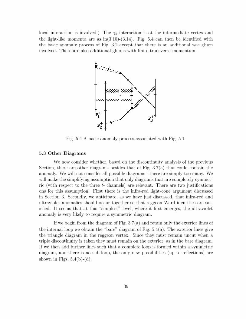
local interaction is involved.) The γ5 interaction is at the intermediate vertex and

the light-like momenta are as in(3.10)-(3.14). Fig. 5.4 can then be identified withthe basic anomaly process of Fig. 3.2 except that there is an additional wee gluoninvolved. There are also additional gluons with finite transverse momentum.

Fig. 5.4 A basic anomaly process associated with Fig. 5.1.

5.3 Other Diagrams

We now consider whether, based on the discontinuity analysis of the previousSection, there are other diagrams besides that of Fig. 3.7(a) that could contain theanomaly. We will not consider all possible diagrams - there are simply too many. Wewill make the simplifying assumption that only diagrams that are completely symmet-ric (with respect to the three t- channels) are relevant. There are two justificationsons for this assumption. First there is the infra-red light-cone argument discussedin Section 3. Secondly, we anticipate, as we have just discussed, that infra-red andultraviolet anomalies should occur together so that reggeon Ward identities are sat-isfied. It seems that at this “simplest” level, where it first emerges, the ultravioletanomaly is very likely to require a symmetric diagram.

If we begin from the diagram of Fig. 3.7(a) and retain only the exterior lines of

the internal loop we obtain the “bare” diagram of Fig. 5.4(a). The exterior lines givethe triangle diagram in the reggeon vertex. Since they must remain uncut when atriple discontinuity is taken they must remain on the exterior, as in the bare diagram.If we then add further lines such that a complete loop is formed within a symmetricdiagram, and there is no sub-loop, the only new possibilities (up to reflections) are

shown in Figs. 5.4(b)-(d).

39

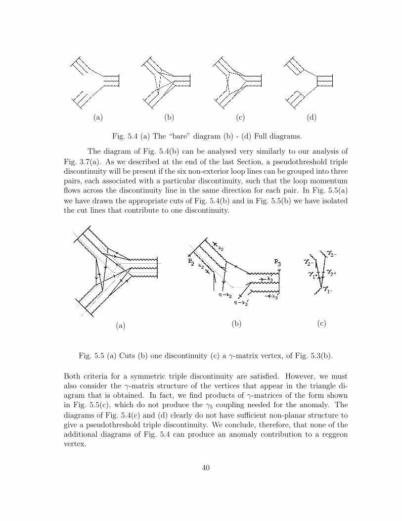
(a) (b) (c) (d)

Fig. 5.4 (a) The “bare” diagram (b) - (d) Full diagrams.

The diagram of Fig. 5.4(b) can be analysed very similarly to our analysis of

Fig. 3.7(a). As we described at the end of the last Section, a pseudothreshold triplediscontinuity will be present if the six non-exterior loop lines can be grouped into threepairs, each associated with a particular discontinuity, such that the loop momentumflows across the discontinuity line in the same direction for each pair. In Fig. 5.5(a)

we have drawn the appropriate cuts of Fig. 5.4(b) and in Fig. 5.5(b) we have isolatedthe cut lines that contribute to one discontinuity.

(a) (b) (c)

Fig. 5.5 (a) Cuts (b) one discontinuity (c) a γ-matrix vertex, of Fig. 5.3(b).

Both criteria for a symmetric triple discontinuity are satisfied. However, we mustalso consider the γ-matrix structure of the vertices that appear in the triangle di-agram that is obtained. In fact, we find products of γ-matrices of the form shownin Fig. 5.5(c), which do not produce the γ5 coupling needed for the anomaly. The

diagrams of Fig. 5.4(c) and (d) clearly do not have sufficient non-planar structure togive a pseudothreshold triple discontinuity. We conclude, therefore, that none of theadditional diagrams of Fig. 5.4 can produce an anomaly contribution to a reggeonvertex.

40

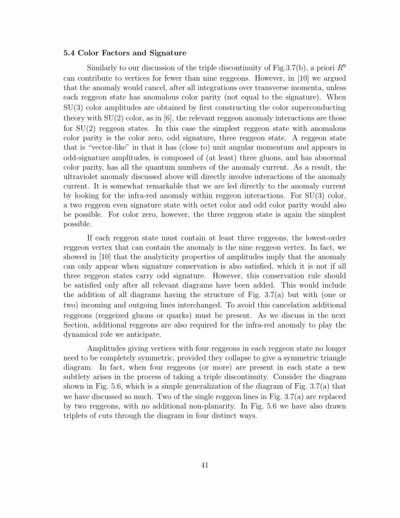
5.4 Color Factors and Signature

Similarly to our discussion of the triple discontinuity of Fig.3.7(b), a priori R9

can contribute to vertices for fewer than nine reggeons. However, in [10] we arguedthat the anomaly would cancel, after all integrations over transverse momenta, unlesseach reggeon state has anomalous color parity (not equal to the signature). When

SU(3) color amplitudes are obtained by first constructing the color superconducting

theory with SU(2) color, as in [6], the relevant reggeon anomaly interactions are those

for SU(2) reggeon states. In this case the simplest reggeon state with anomalouscolor parity is the color zero, odd signature, three reggeon state. A reggeon statethat is “vector-like” in that it has (close to) unit angular momentum and appears in

odd-signature amplitudes, is composed of (at least) three gluons, and has abnormalcolor parity, has all the quantum numbers of the anomaly current. As a result, theultraviolet anomaly discussed above will directly involve interactions of the anomalycurrent. It is somewhat remarkable that we are led directly to the anomaly currentby looking for the infra-red anomaly within reggeon interactions. For SU(3) color,a two reggeon even signature state with octet color and odd color parity would alsobe possible. For color zero, however, the three reggeon state is again the simplestpossible.

If each reggeon state must contain at least three reggeons, the lowest-orderreggeon vertex that can contain the anomaly is the nine reggeon vertex. In fact, weshowed in [10] that the analyticity properties of amplitudes imply that the anomalycan only appear when signature conservation is also satisfied, which it is not if allthree reggeon states carry odd signature. However, this conservation rule shouldbe satisfied only after all relevant diagrams have been added. This would includethe addition of all diagrams having the structure of Fig. 3.7(a) but with (one or

two) incoming and outgoing lines interchanged. To avoid this cancelation additional

reggeons (reggeized gluons or quarks) must be present. As we discuss in the nextSection, additional reggeons are also required for the infra-red anomaly to play thedynamical role we anticipate.

Amplitudes giving vertices with four reggeons in each reggeon state no longerneed to be completely symmetric, provided they collapse to give a symmetric trianglediagram. In fact, when four reggeons (or more) are present in each state a newsubtlety arises in the process of taking a triple discontinuity. Consider the diagramshown in Fig. 5.6, which is a simple generalization of the diagram of Fig. 3.7(a) that

we have discussed so much. Two of the single reggeon lines in Fig. 3.7(a) are replacedby two reggeons, with no additional non-planarity. In Fig. 5.6 we have also drawntriplets of cuts through the diagram in four distinct ways.

41

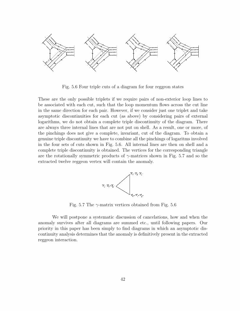
Fig. 5.6 Four triple cuts of a diagram for four reggeon states

These are the only possible triplets if we require pairs of non-exterior loop lines tobe associated with each cut, such that the loop momentum flows across the cut linein the same direction for each pair. However, if we consider just one triplet and takeasymptotic discontinuities for each cut (as above) by considering pairs of externallogarithms, we do not obtain a complete triple discontinuity of the diagram. Thereare always three internal lines that are not put on shell. As a result, one or more, ofthe pinchings does not give a complete, invariant, cut of the diagram. To obtain agenuine triple discontinuity we have to combine all the pinchings of logaritms involvedin the four sets of cuts shown in Fig. 5.6. All internal lines are then on shell and acomplete triple discontinuity is obtained. The vertices for the corresponding triangleare the rotationally symmetric products of γ-matrices shown in Fig. 5.7 and so theextracted twelve reggeon vertex will contain the anomaly.

Fig. 5.7 The γ-matrix vertices obtained from Fig. 5.6

We will postpone a systematic discussion of cancelations, how and when theanomaly survives after all diagrams are summed etc., until following papers. Ourpriority in this paper has been simply to find diagrams in which an asymptotic dis-continuity analysis determines that the anomaly is definitively present in the extractedreggeon interaction.

42

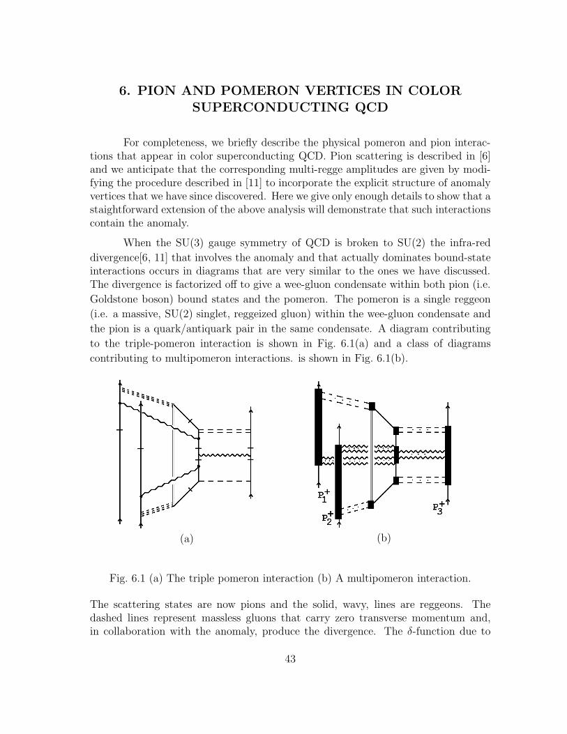
6. PION AND POMERON VERTICES IN COLOR

SUPERCONDUCTING QCD

For completeness, we briefly describe the physical pomeron and pion interac-tions that appear in color superconducting QCD. Pion scattering is described in [6]and we anticipate that the corresponding multi-regge amplitudes are given by modi-fying the procedure described in [11] to incorporate the explicit structure of anomalyvertices that we have since discovered. Here we give only enough details to show that astaightforward extension of the above analysis will demonstrate that such interactionscontain the anomaly.

When the SU(3) gauge symmetry of QCD is broken to SU(2) the infra-red

divergence[6, 11] that involves the anomaly and that actually dominates bound-stateinteractions occurs in diagrams that are very similar to the ones we have discussed.The divergence is factorized off to give a wee-gluon condensate within both pion (i.e.

Goldstone boson) bound states and the pomeron. The pomeron is a single reggeon

(i.e. a massive, SU(2) singlet, reggeized gluon) within the wee-gluon condensate and

the pion is a quark/antiquark pair in the same condensate. A diagram contributing

to the triple-pomeron interaction is shown in Fig. 6.1(a) and a class of diagrams

contributing to multipomeron interactions. is shown in Fig. 6.1(b).

(a) (b)

Fig. 6.1 (a) The triple pomeron interaction (b) A multipomeron interaction.

The scattering states are now pions and the solid, wavy, lines are reggeons. Thedashed lines represent massless gluons that carry zero transverse momentum and,in collaboration with the anomaly, produce the divergence. The δ-function due to

43

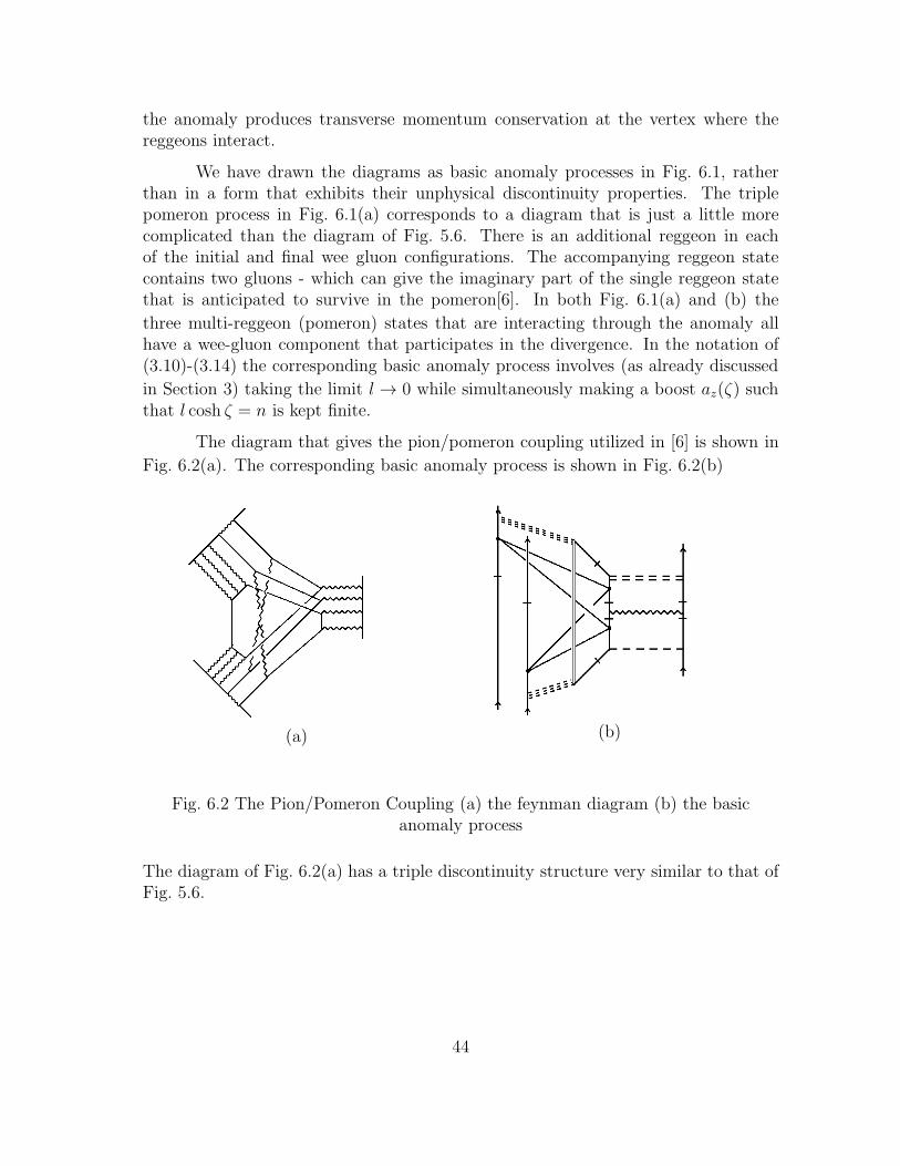
the anomaly produces transverse momentum conservation at the vertex where thereggeons interact.

We have drawn the diagrams as basic anomaly processes in Fig. 6.1, ratherthan in a form that exhibits their unphysical discontinuity properties. The triplepomeron process in Fig. 6.1(a) corresponds to a diagram that is just a little morecomplicated than the diagram of Fig. 5.6. There is an additional reggeon in eachof the initial and final wee gluon configurations. The accompanying reggeon statecontains two gluons - which can give the imaginary part of the single reggeon statethat is anticipated to survive in the pomeron[6]. In both Fig. 6.1(a) and (b) the

three multi-reggeon (pomeron) states that are interacting through the anomaly allhave a wee-gluon component that participates in the divergence. In the notation of(3.10)-(3.14) the corresponding basic anomaly process involves (as already discussed

in Section 3) taking the limit l → 0 while simultaneously making a boost az(ζ) suchthat l cosh ζ = n is kept finite.

The diagram that gives the pion/pomeron coupling utilized in [6] is shown in

Fig. 6.2(a). The corresponding basic anomaly process is shown in Fig. 6.2(b)

(a) (b)

Fig. 6.2 The Pion/Pomeron Coupling (a) the feynman diagram (b) the basicanomaly process

The diagram of Fig. 6.2(a) has a triple discontinuity structure very similar to that ofFig. 5.6.

44

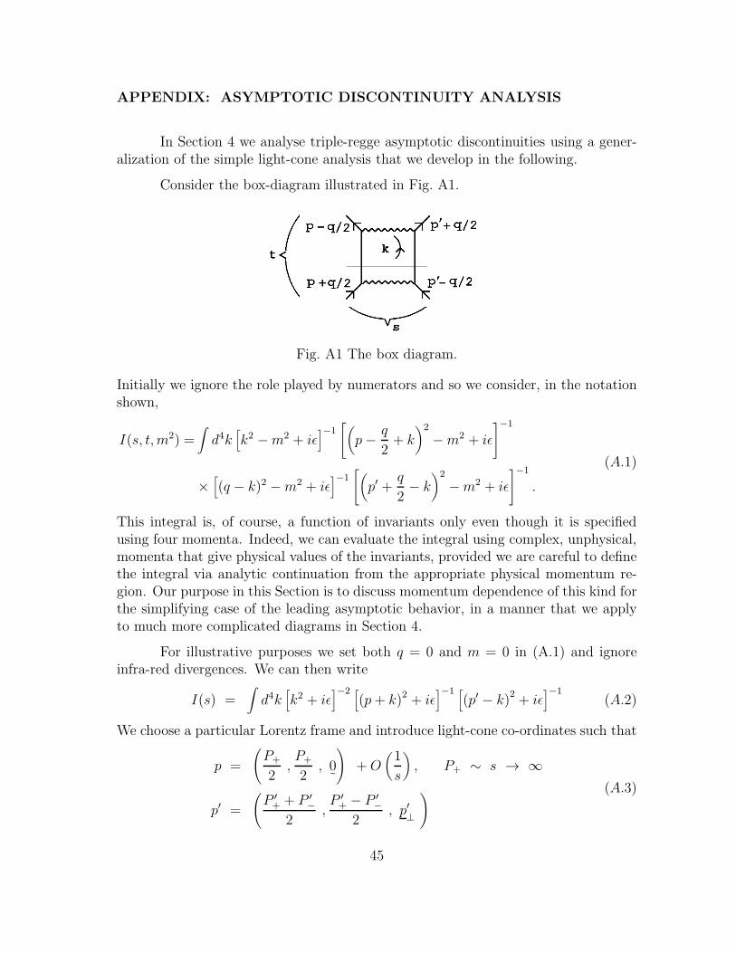
APPENDIX: ASYMPTOTIC DISCONTINUITY ANALYSIS

In Section 4 we analyse triple-regge asymptotic discontinuities using a gener-alization of the simple light-cone analysis that we develop in the following.

Consider the box-diagram illustrated in Fig. A1.

Fig. A1 The box diagram.

Initially we ignore the role played by numerators and so we consider, in the notationshown,

I(s, t,m2) =∫

d4k[

k2 −m2 + iǫ]−1

[

(

p− q

2+ k

)2

−m2 + iǫ

]−1

×[

(q − k)2 −m2 + iǫ]−1

[

(

p′ +q

2− k

)2

−m2 + iǫ

]−1

.

(A.1)

This integral is, of course, a function of invariants only even though it is specifiedusing four momenta. Indeed, we can evaluate the integral using complex, unphysical,momenta that give physical values of the invariants, provided we are careful to definethe integral via analytic continuation from the appropriate physical momentum re-gion. Our purpose in this Section is to discuss momentum dependence of this kind forthe simplifying case of the leading asymptotic behavior, in a manner that we applyto much more complicated diagrams in Section 4.

For illustrative purposes we set both q = 0 and m = 0 in (A.1) and ignoreinfra-red divergences. We can then write

I(s) =∫

d4k[

k2 + iǫ]−2 [

(p+ k)2 + iǫ]−1 [

(p′ − k)2+ iǫ

]−1(A.2)

We choose a particular Lorentz frame and introduce light-cone co-ordinates such that

p =

(

P+

2,P+

2, 0˜

)

+O(

1

s

)

, P+ ∼ s → ∞

p′ =

(

P ′+ + P ′

−

2,P ′+ − P ′

−

2, p′

⊥

)(A.3)

45

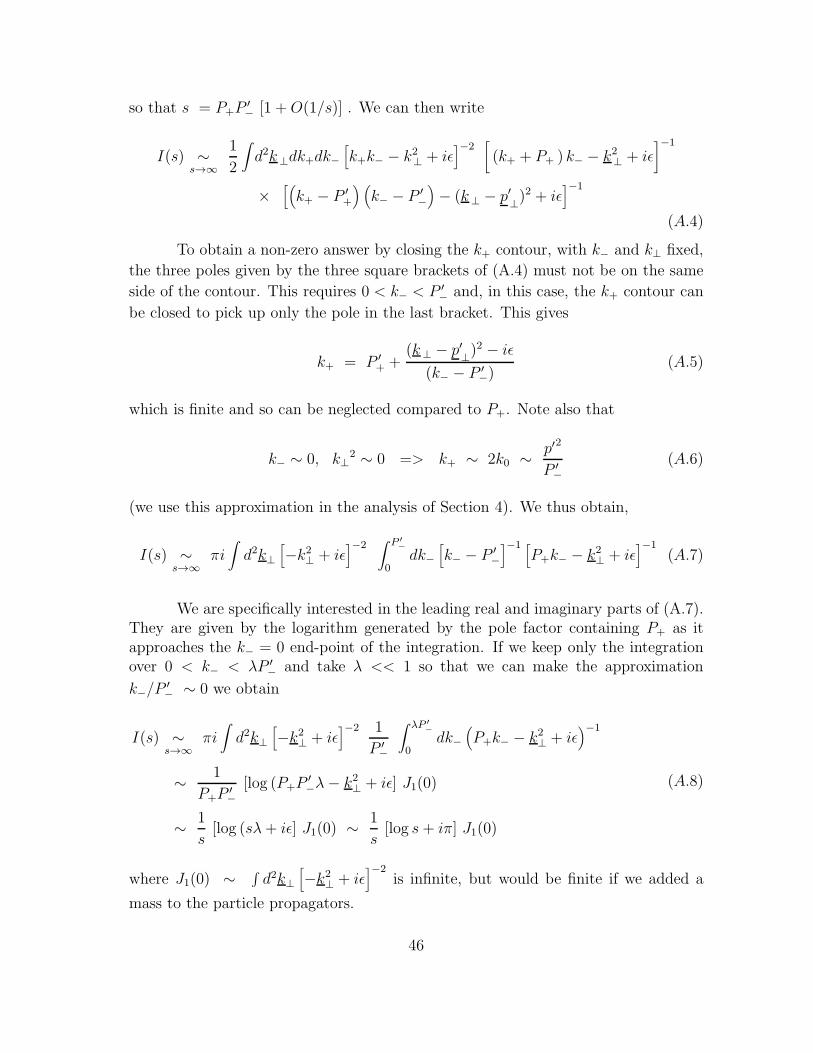
so that s = P+P′− [1 +O(1/s)] . We can then write

I(s) ∼s→∞

1

2

∫

d2k⊥dk+dk−[

k+k− − k2⊥ + iǫ]−2

[

(k+ + P+ ) k− − k2⊥ + iǫ]−1

×[(

k+ − P ′+

) (

k− − P ′−

)

− (k⊥ − p′⊥)2 + iǫ

]−1

(A.4)

To obtain a non-zero answer by closing the k+ contour, with k− and k⊥ fixed,

the three poles given by the three square brackets of (A.4) must not be on the same

side of the contour. This requires 0 < k− < P ′− and, in this case, the k+ contour can

be closed to pick up only the pole in the last bracket. This gives

k+ = P ′+ +

(k⊥ − p′⊥)2 − iǫ

(k− − P ′−)

(A.5)

which is finite and so can be neglected compared to P+. Note also that

k− ∼ 0, k⊥2 ∼ 0 => k+ ∼ 2k0 ∼ p′2

P ′−

(A.6)

(we use this approximation in the analysis of Section 4). We thus obtain,

I(s) ∼s→∞

πi∫

d2k⊥[

−k2⊥ + iǫ]−2

∫ P ′−

0dk−

[

k− − P ′−

]−1 [

P+k− − k2⊥ + iǫ]−1

(A.7)

We are specifically interested in the leading real and imaginary parts of (A.7).They are given by the logarithm generated by the pole factor containing P+ as itapproaches the k− = 0 end-point of the integration. If we keep only the integrationover 0 < k− < λP ′

− and take λ << 1 so that we can make the approximation

k−/P′− ∼ 0 we obtain

I(s) ∼s→∞

πi∫

d2k⊥[

−k2⊥ + iǫ]−2 1

P ′−

∫ λP ′−

0dk−

(

P+k− − k2⊥ + iǫ)−1

∼ 1

P+P ′−

[log (P+P′−λ− k2⊥ + iǫ] J1(0)

∼ 1

s[log (sλ+ iǫ] J1(0) ∼ 1

s[log s+ iπ] J1(0)

(A.8)

where J1(0) ∼ ∫

d2k⊥[

−k2⊥ + iǫ]−2

is infinite, but would be finite if we added a

mass to the particle propagators.

46

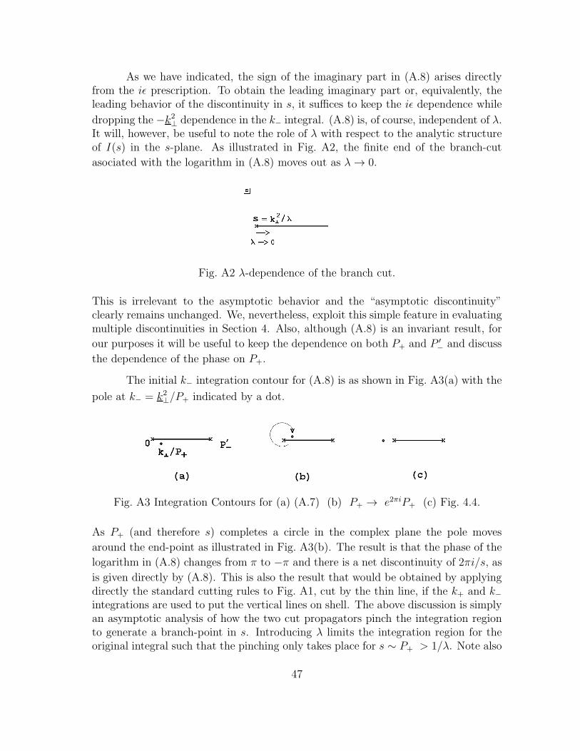
As we have indicated, the sign of the imaginary part in (A.8) arises directlyfrom the iǫ prescription. To obtain the leading imaginary part or, equivalently, theleading behavior of the discontinuity in s, it suffices to keep the iǫ dependence while

dropping the −k2⊥ dependence in the k− integral. (A.8) is, of course, independent of λ.It will, however, be useful to note the role of λ with respect to the analytic structureof I(s) in the s-plane. As illustrated in Fig. A2, the finite end of the branch-cut

asociated with the logarithm in (A.8) moves out as λ→ 0.

Fig. A2 λ-dependence of the branch cut.

This is irrelevant to the asymptotic behavior and the “asymptotic discontinuity”clearly remains unchanged. We, nevertheless, exploit this simple feature in evaluatingmultiple discontinuities in Section 4. Also, although (A.8) is an invariant result, for

our purposes it will be useful to keep the dependence on both P+ and P ′− and discuss

the dependence of the phase on P+.

The initial k− integration contour for (A.8) is as shown in Fig. A3(a) with the

pole at k− = k2⊥/P+ indicated by a dot.

Fig. A3 Integration Contours for (a) (A.7) (b) P+ → e2πiP+ (c) Fig. 4.4.

As P+ (and therefore s) completes a circle in the complex plane the pole moves

around the end-point as illustrated in Fig. A3(b). The result is that the phase of the

logarithm in (A.8) changes from π to −π and there is a net discontinuity of 2πi/s, as

is given directly by (A.8). This is also the result that would be obtained by applyingdirectly the standard cutting rules to Fig. A1, cut by the thin line, if the k+ and k−integrations are used to put the vertical lines on shell. The above discussion is simplyan asymptotic analysis of how the two cut propagators pinch the integration regionto generate a branch-point in s. Introducing λ limits the integration region for theoriginal integral such that the pinching only takes place for s ∼ P+ > 1/λ. Note also

47

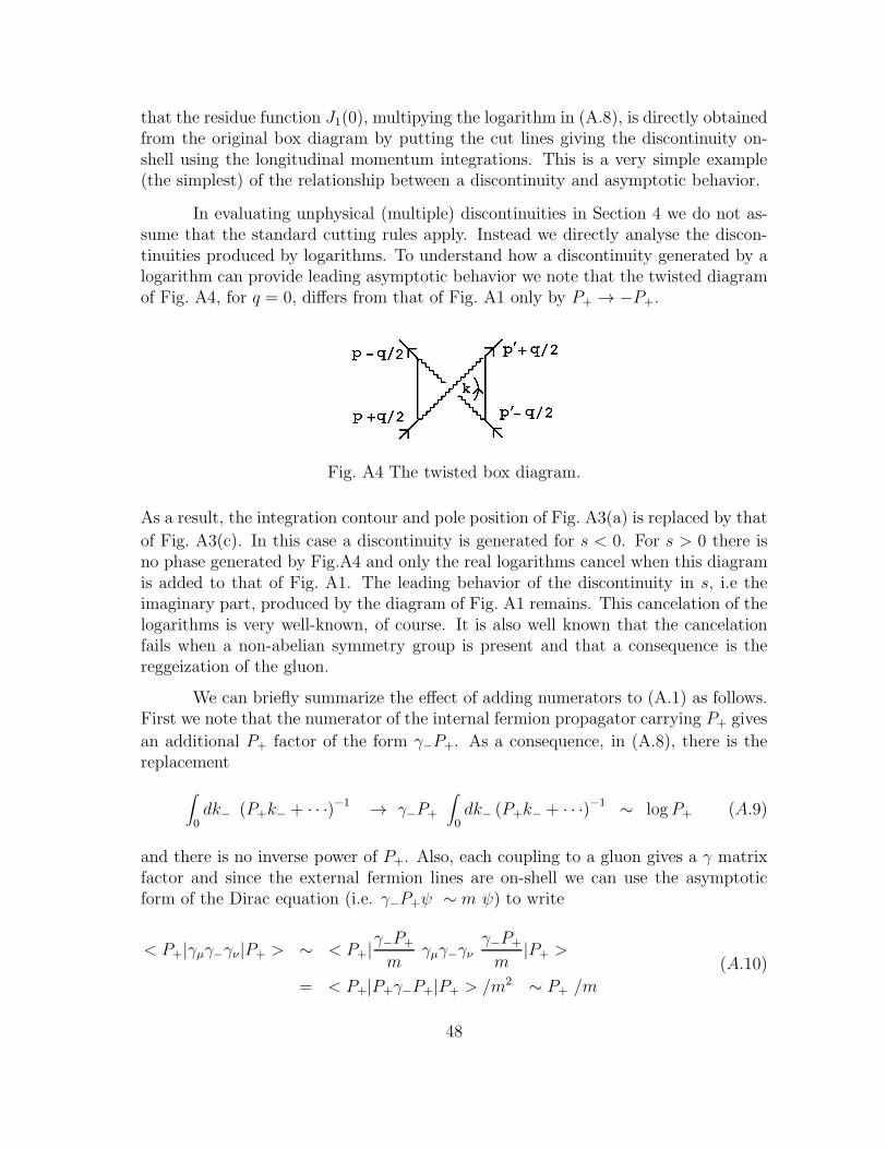
that the residue function J1(0), multipying the logarithm in (A.8), is directly obtainedfrom the original box diagram by putting the cut lines giving the discontinuity on-shell using the longitudinal momentum integrations. This is a very simple example(the simplest) of the relationship between a discontinuity and asymptotic behavior.

In evaluating unphysical (multiple) discontinuities in Section 4 we do not as-sume that the standard cutting rules apply. Instead we directly analyse the discon-tinuities produced by logarithms. To understand how a discontinuity generated by alogarithm can provide leading asymptotic behavior we note that the twisted diagramof Fig. A4, for q = 0, differs from that of Fig. A1 only by P+ → −P+.

Fig. A4 The twisted box diagram.

As a result, the integration contour and pole position of Fig. A3(a) is replaced by that

of Fig. A3(c). In this case a discontinuity is generated for s < 0. For s > 0 there isno phase generated by Fig.A4 and only the real logarithms cancel when this diagramis added to that of Fig. A1. The leading behavior of the discontinuity in s, i.e theimaginary part, produced by the diagram of Fig. A1 remains. This cancelation of thelogarithms is very well-known, of course. It is also well known that the cancelationfails when a non-abelian symmetry group is present and that a consequence is thereggeization of the gluon.

We can briefly summarize the effect of adding numerators to (A.1) as follows.First we note that the numerator of the internal fermion propagator carrying P+ gives

an additional P+ factor of the form γ−P+. As a consequence, in (A.8), there is thereplacement

∫

0dk− (P+k− + · · ·)−1 → γ−P+

∫

0dk− (P+k− + · · ·)−1 ∼ logP+ (A.9)

and there is no inverse power of P+. Also, each coupling to a gluon gives a γ matrixfactor and since the external fermion lines are on-shell we can use the asymptoticform of the Dirac equation (i.e. γ−P+ψ ∼ m ψ) to write

< P+|γµγ−γν|P+ > ∼ < P+|γ−P+

mγµγ−γν

γ−P+

m|P+ >

= < P+|P+γ−P+|P+ > /m2 ∼ P+ /m

(A.10)

48

This gives another power of P+ (∼ s) provided that the corresponding factor of P ′−

is present in the finite momentum part of the scattering process. Not surprisinglythis factor emerges from that part which would dominate if P ′

− were large. However,

we want to emphasize that this selection is made only by the need to form a Lorentzinvariant amplitude from the non-invariant large momentum process.

Finally we note that the above analysis goes through with very little modifi-

cation if we take both m2 and q to be non-zero so that (A.2) will not be infra-reddivergent.

49

References

[1] V. N. Gribov, Nucl. Phys. B139, 1 (1978), G. ’t Hooft, Nucl. Phys. Proc. Suppl.

B74, 413 (1999).

[2] M. F. Atiyah, in Anomalies, Geometry and Topology, edited by W. A. Bardeen

and A. R. White (World Scientific, Singapore, 1985); R. Jackiw, ibid. and inEffects of Dirac’s Negative Energy Sea Quantum Numbers, Dirac Prize lecture,March 1999, hep-th/9903255.

[3] G. ’t Hooft, Phys. Rep. 142, 357 (1986).

[4] D. Diakonov and V. Yu. Petrov, Nucl. Phys. B272, 457 (1986).

[5] H. Leutwyler and A. Smilga, Phys. Rev. D46, 5607 (1992).

[6] A. R. White, hep-ph/0202169.

[7] E. A. Kuraev, L. N. Lipatov, V. S. Fadin, Sov. Phys. JETP 45, 199 (1977);

J. B. Bronzan and R. L. Sugar, Phys. Rev. D17, 585 (1978), this paper organizesinto reggeon diagrams the results from H. Cheng and C. Y. Lo, Phys. Rev. D13,1131 (1976), D15, 2959 (1977); V. S. Fadin and V. E. Sherman, Sov. Phys. JETP

45, 861 (1978); V. S. Fadin and L. N. Lipatov, Nucl. Phys. B477, 767 (1996)

and further references therein; J. Bartels, Z. Phys. C60, 471 (1993) and further

references therein; A. R. White, Int. J. Mod. Phys. A8, 4755 (1993).

[8] P. Goddard and A. R. White, Nucl. Phys. B17, 1, 45 (1970). As in [10] weemphasize that the full triple-regge limit is distinct from the “triple-regge” limitof the one-particle inclusive cross-section that is a “non-flip helicity-pole” limit.

[9] A. R. White, Phys. Rev. D29, 1435 (1984).

[10] A. R. White, Phys. Rev. D63 016007, (2001).

[11] A. R. White, Phys. Rev. D58, 074008 (1998).

[12] A. R. White, Nucl. Phys. Proc. Suppl. 96, 277-286 (2001) - hep-ph/0008267;see also Lectures in the Proceedings of the Theory Institute on Deep-InelasticDiffraction, Argonne National Laboratory (1998).

[13] A. A. Migdal, A. M. Polyakov and K. A. Ter-Martirosyan, Zh. Eksp. Teor. Fiz.

67, 84 (1974); H. D. I. Abarbanel and J. B. Bronzan, Phys. Rev.D9, 2397 (1974).

[14] V. S. Fadin and L. N. Lipatov, Nucl. Phys. B406, 259 (1993).

50

[15] O. Steinmann, Helv. Phys. Acta. 33 257, 347 (1960); H. Epstein, in Structural

Analysis Of Collision Amplitudes edited by R. Balian and D. Iagolnitzer (Ams-

terdam 1976), and references therein.

[16] A. R. White, hep-ph/0002303 - The Past and Future of S-Matrix Theory in

Scattering, edited by E. R. Pike and P. Sabatier (Academic Press, London) andreferences therein.

[17] S. Coleman and B. Grossman, Nucl. Phys. B203, 205 (1982).

51