Department of Automatic Control

Artificial Intelligence and Terrain Handling of a Hexapod Robot

Markus Malmros

Amanda Eriksson

MSc Thesis TFRT-6010 ISSN 0280-5316

Department of Automatic Control Lund University Box 118 SE-221 00 LUND Sweden

© 2016 by Markus Malmros & Amanda Eriksson. All rights reserved. Printed in Sweden by Tryckeriet i E-huset Lund 2016

Abstract

The focus of this master’s thesis has been getting a six-legged robot to au-tonomously navigate around a room with obstacles. To make this possible a time-of-flight camera has been implemented in order to map the environment. Two forcesensing resistors were also mounted on the front legs to sense if the legs are in con-tact with the ground. The information from the sensors together with a path planningalgorithm and new leg trajectory calculations have resulted in new abilities for therobot.

During the project comparisons between different hardware, tools and algo-rithms have been made in order to choose the ones fitting the requirements best.Tests have also been made, both on the robot and in simulations to investigate howwell the models work.

The results are path planning algorithms and a terrain handling feature thatworks very well in simulations and satisfyingly in the real world. One of the mainbottlenecks during the project has been the lack of computational power of the hard-ware. With a stronger processor, the algorithms would work more efficiently andcould be developed further to increase the precision of the environment map andthe path planning algorithms.

3

Acknowledgements

First of all we would like to thank Combine Control Systems and our supervisorthere, Simon Yngve, for giving us the possibility of writing this thesis for them andalso for providing us with the equipment needed and helping us in the times we gotstuck. A special thanks goes to Sara Gustafzelius and Andreas Tågerud for all thehelp with the camera implementation and computer hacking stuff.

We would also like to thank the Department of Automatic Control, at LundUniversity for providing us with tools and hardware during this master thesis. Oursupervisor at the department, Anders Robertsson, has guided us through this projectand helped us a lot with his ideas during our weekly meetings.

Finally we would like to thank Dan Thilderkvist and Sebastian Svensson for theprevious work they did that made our work possible and for answering our questionsabout the Hexapod.

5

Acronyms

UAV Unmanned Aerial Vehicle

IMU Inertial Measurement Unit

RGB-D Red Green Blue - Depth

TOF Time-of-Flight

FSR Force Sensing Resistor

RANSAC Random Sample Consensus

RANSOP Random Sample Optimization

RRT Rapidly Exploring Random Trees

PRM Probabilistic Road Map

BFS Breadth First Search

DFS Depth First Search

LIDAR Light Detection and Ranging

UCS Uniform Cost Search

SLAM Simultaneously Localization And Mapping

CAD Computer Aided Design

7

Contents

1. Introduction 111.1 Background . . . . . . . . . . . . . . . . . . . . . . . . . . . . 111.2 Previous Work . . . . . . . . . . . . . . . . . . . . . . . . . . . 111.3 Goals . . . . . . . . . . . . . . . . . . . . . . . . . . . . . . . . 121.4 Resources and Division of Labor . . . . . . . . . . . . . . . . . 131.5 Tools . . . . . . . . . . . . . . . . . . . . . . . . . . . . . . . . 131.6 Outline . . . . . . . . . . . . . . . . . . . . . . . . . . . . . . . 13

2. Theory 152.1 Modeling and Simulation Software . . . . . . . . . . . . . . . . 152.2 Force Sensing Resistor . . . . . . . . . . . . . . . . . . . . . . 162.3 Time-of-Flight (depth) Camera . . . . . . . . . . . . . . . . . . 162.4 Depth Map To Coordinates . . . . . . . . . . . . . . . . . . . . 182.5 Random Sample Consensus (RANSAC) . . . . . . . . . . . . . 192.6 Random Sample Optimization (RANSOP) . . . . . . . . . . . . 192.7 Planning Problem Formulation . . . . . . . . . . . . . . . . . . 222.8 Non-holonomic System . . . . . . . . . . . . . . . . . . . . . . 232.9 Motion Planning . . . . . . . . . . . . . . . . . . . . . . . . . . 232.10 Overview of Planning in Continuous Space . . . . . . . . . . . . 232.11 Road Map . . . . . . . . . . . . . . . . . . . . . . . . . . . . . 242.12 Search Methods in a Discrete State Space Graph . . . . . . . . . 28

3. Method 343.1 Simulink Model . . . . . . . . . . . . . . . . . . . . . . . . . . 343.2 Friction Modeling in SimMechanics . . . . . . . . . . . . . . . 383.3 Choice of Simulation Software . . . . . . . . . . . . . . . . . . 383.4 Setting Up the Hexapod in V-REP . . . . . . . . . . . . . . . . . 383.5 Mapping sensors . . . . . . . . . . . . . . . . . . . . . . . . . . 413.6 Camera Implementation . . . . . . . . . . . . . . . . . . . . . . 433.7 Overview of Autonomous Mode . . . . . . . . . . . . . . . . . 443.8 Real-Time Multi-threading . . . . . . . . . . . . . . . . . . . . 463.9 Positioning of the Hexapod . . . . . . . . . . . . . . . . . . . . 46

9

Contents

3.10 Mapping and Planning Overview . . . . . . . . . . . . . . . . . 483.11 Planning . . . . . . . . . . . . . . . . . . . . . . . . . . . . . . 513.12 Search . . . . . . . . . . . . . . . . . . . . . . . . . . . . . . . 513.13 Path Following and Feedback . . . . . . . . . . . . . . . . . . . 533.14 Remote Control Changes . . . . . . . . . . . . . . . . . . . . . 553.15 Terrain Handling . . . . . . . . . . . . . . . . . . . . . . . . . . 573.16 Electrical Assembly . . . . . . . . . . . . . . . . . . . . . . . . 63

4. Results 654.1 RANSAC and RANSOP . . . . . . . . . . . . . . . . . . . . . . 664.2 Mapping . . . . . . . . . . . . . . . . . . . . . . . . . . . . . . 714.3 Complete Planning Tests . . . . . . . . . . . . . . . . . . . . . 724.4 Force Sensors . . . . . . . . . . . . . . . . . . . . . . . . . . . 77

5. Discussion and Conclusions 785.1 Discussion . . . . . . . . . . . . . . . . . . . . . . . . . . . . . 785.2 Conclusions . . . . . . . . . . . . . . . . . . . . . . . . . . . . 865.3 Future Improvements . . . . . . . . . . . . . . . . . . . . . . . 87

Bibliography 89

10

1

Introduction

1.1 Background

The growing trend of developing and using automated, unmanned vehicles couldbe very useful for making the work in dangerous and non human-friendly envi-ronments safer and more efficient. A robot could for example be used in the ruinsafter a big earthquake to find survivors and possible paths for emergency work-ers. This is one application that has inspired the work and the goals of this thesis.The project is based on a previous master thesis for Combine Control Systems inLund where locomotion and movement patterns were developed for a six-leggedrobot, also known as hexapod. Since the hexapod is stable, has many legs and isrelatively small it could work very well together with sensors and a path planningalgorithm for applications in non human-friendly environments. An autonomousterrain handling hexapod is also a great possibility for Combine Control Systems todemonstrate their work and a way to present their competence and business idea ata technical fair.

1.2 Previous Work

The initial development of the hexapod used in this project was made by two mas-ter students, Dan Thilderkvist and Sebastian Svensson. They mounted a six-leggedrobot and programmed a micro-controller to work with a remote control. They alsodeveloped a feature for stabilizing the body of the robot as the angle of the groundchanged. This was done by measuring the body angle with an IMU (Inertial Mea-surement Unit). The stabilization feature could however only be used when the robotwas standing still. The software development process was performed according toprinciples in model-based design in Simulink and Matlab.

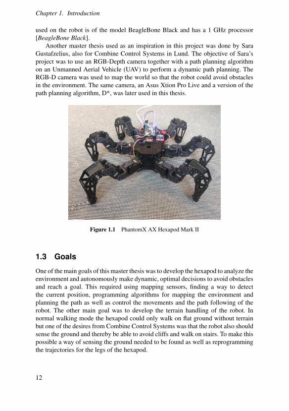
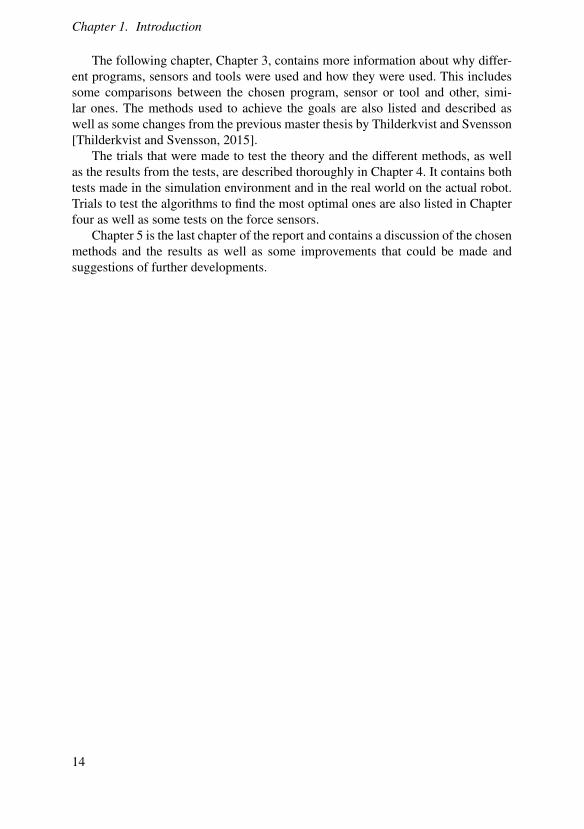
The robot used is of the model PhantomX AX Hexapod Mark II from InterbotixLabs, see Figure 1.1. It has six legs, uses three servos per leg and thereby provides 18degrees of freedom. The hand-held control is wireless and communicates with thehexapod by using XBee modules [Thilderkvist and Svensson, 2015]. The computer

11

Chapter 1. Introduction

used on the robot is of the model BeagleBone Black and has a 1 GHz processor[BeagleBone Black].

Another master thesis used as an inspiration in this project was done by SaraGustafzelius, also for Combine Control Systems in Lund. The objective of Sara’sproject was to use an RGB-Depth camera together with a path planning algorithmon an Unmanned Aerial Vehicle (UAV) to perform a dynamic path planning. TheRGB-D camera was used to map the world so that the robot could avoid obstaclesin the environment. The same camera, an Asus Xtion Pro Live and a version of thepath planning algorithm, D*, was later used in this thesis.

Figure 1.1 PhantomX AX Hexapod Mark II

1.3 Goals

One of the main goals of this master thesis was to develop the hexapod to analyze theenvironment and autonomously make dynamic, optimal decisions to avoid obstaclesand reach a goal. This required using mapping sensors, finding a way to detectthe current position, programming algorithms for mapping the environment andplanning the path as well as control the movements and the path following of therobot. The other main goal was to develop the terrain handling of the robot. Innormal walking mode the hexapod could only walk on flat ground without terrainbut one of the desires from Combine Control Systems was that the robot also shouldsense the ground and thereby be able to avoid cliffs and walk on stairs. To make thispossible a way of sensing the ground needed to be found as well as reprogrammingthe trajectories for the legs of the hexapod.

12

1.4 Resources and Division of Labor

1.4 Resources and Division of Labor

To make the project work more efficient the labor was divided between Amanda andMarkus during the thesis. Markus has more of a computer science background witha focus on artificial intelligence, statistics and planning. Therefore he focused onresearching and implementing the systems for performing planning, mapping andpath-following autonomously.

Amanda, on the other hand, has taken more courses in mechatronics, electronicsand embedded systems and therefore focused more on the hardware. That involvedfor example setting up the camera and get it to work with Simulink, find, buy andinstall the force sensors and activate the accelerometer to test whether it could beused as a positioning tool.

1.5 Tools

The two main tools used in this thesis are Matlab [Matlab], with the Simulink envi-ronment [Simulink], and the robot simulator V-REP [coppeliarobotics.com]. Moreabout V-REP and why it was chosen as a simulation tool can be read in Chapter 2and 3.

Figure 1.2 Matlab Simulink Figure 1.3 V-REP

1.6 Outline

The first chapter of the report contains background information to give the reader anintroduction to the rest of the thesis. The purpose of the project and a couple of pre-vious projects that made this thesis possible are also mentioned in the introductionas well as the different goals and constraints that have been followed throughout theproject.

In Chapter 2 the theory behind the methods later used is explained. Some con-cepts and models are also explained to make it easier for the reader to understandthe following chapters. The theory section also contains information about the toolsused, for example V-REP, and explains how the sensors work, both the time-of-flight(depth) camera and the force sensing resistance.

13

Chapter 1. Introduction

The following chapter, Chapter 3, contains more information about why differ-ent programs, sensors and tools were used and how they were used. This includessome comparisons between the chosen program, sensor or tool and other, simi-lar ones. The methods used to achieve the goals are also listed and described aswell as some changes from the previous master thesis by Thilderkvist and Svensson[Thilderkvist and Svensson, 2015].

The trials that were made to test the theory and the different methods, as wellas the results from the tests, are described thoroughly in Chapter 4. It contains bothtests made in the simulation environment and in the real world on the actual robot.Trials to test the algorithms to find the most optimal ones are also listed in Chapterfour as well as some tests on the force sensors.

Chapter 5 is the last chapter of the report and contains a discussion of the chosenmethods and the results as well as some improvements that could be made andsuggestions of further developments.

14

2

Theory

2.1 Modeling and Simulation Software

The main software used in this project to model, simulate and analyze the code andsystems are Mathworks Simulink and V-REP.

Simulink and MatlabSimulink and Matlab are two products from the corporation Mathworks. Togetherthey can be used to create a model of a system and simulate it and/or run it onexternal hardware. External code can be included to the model which makes thecode development process easy and efficient. The software is also good for analyz-ing the results of the simulations [Matlab] [Simulink]. All the code that is used onthe hardware in this project is programmed directly in or is code-generated throughSimulink.

Simulink Code GenerationIn order to write the code from Simulink to the hardware, code generation isrequired. Code generation transforms the source code from the Simulink modelinto executable code that can be run on the hardware. However, this requires theMathworks-tool Embedded Coder [Understanding C Code Generation]. The setupused is based on the setup from the previous master’s thesis on the hexapod by DanThilderkvist and Sebastian Svensson [Thilderkvist and Svensson, 2015].

V-REPV-REP is a robotics simulator with broad capabilities in simulation of mobile robots,factory automation and a tool for fast algorithm development. It is cross-platformcompatible and works on Windows as well as Mac and Linux. V-REP provides threedifferent physics-engines for dynamic calculations and collision detection betweenmeshes. A wide range of sensors and terrain capabilities are also included [Enablingthe Remote API - client side].

15

Chapter 2. Theory

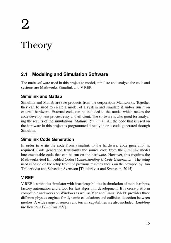
2.2 Force Sensing Resistor

The force sensing resistors, FSRs, used in this project are manufactured by the com-pany Interlinc Electronics. They are 5 mm in diameter and have a thickness of 0.30mm, hence, they are small enough to fit under the feet of the hexapod. When a forceis applied to the circular part of the sensor the resistance is lowered and with in-creasing force the resistance is decreasing even more [FSR Force Sensing ResistorIntegration Guide and Evaluation Parts Catalog]. The two ends of the sensors areconnected according to the circuit in Figure 2.2. One of the sensor pins are con-nected to VDD and the other pin is connected to both ground together via a 10 kOhm resistor and to one of the analog inputs of the BeagleBone Black. The changesof the analog input pin can thereafter be read and the information can be used toprogram the walking pattern of the hexapod.

Figure 2.1 The force sensing resistor[Picture of FSR].

Vdd

10k

FSR

VOUT

Figure 2.2 The electrical circuit of thesensor connection.

2.3 Time-of-Flight (depth) Camera

Time-of-flight cameras have reached an upswing during the last couple of yearswhen they have become cheap consumer products, mainly from the introductionof the Microsoft Kinect camera. The cameras are a compact and convenient wayof gathering 3D information about the world. They offer high sample rates andaccurate depth readings.

A TOF camera works by emitting pulses of infrared light which illuminates theenvironment. The wave length is usually around 850 nm and not visible to the hu-man eye. The light spreads across the environment and will be reflected on objects.The reflected light arrives back at a photosensitive imaging sensor designed for theinfrared spectrum. The time of flight of the light is measured. Since the speed oflight is known this information can be used to calculate the distance to a certainpoint in space. This is done simultaneously for all pixels in the image sensor ma-

16

2.3 Time-of-Flight (depth) Camera

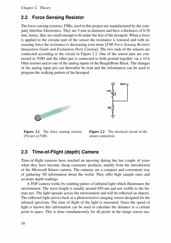
trix. The equation used for calculating the depth is presented in Equation 2.1 whered is the depth distance in the current pixel [Li, 2014]. The speed of light is denotedc, Dt is the amount of time during which the illumination occurs, that is, pulse width.The reflected energy is measured by two out of phase windows, C1 and C2. Electri-cal charges accumulated during these two windows are integrated and denoted Q1and Q2. Figure 2.3 illustrates the time aspects of measuring the depth distance.

d =12

cDtQ2

Q1 +Q2(2.1)

Figure 2.3 Time-of-flight time integration [Li, 2014]

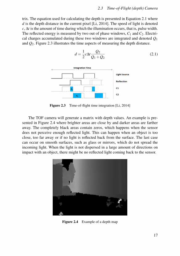
The TOF camera will generate a matrix with depth values. An example is pre-sented in Figure 2.4 where brighter areas are close by and darker areas are fartheraway. The completely black areas contain zeros, which happens when the sensordoes not perceive enough reflected light. This can happen when an object is tooclose, too far away or if no light is reflected back from the surface. The last casecan occur on smooth surfaces, such as glass or mirrors, which do not spread theincoming light. When the light is not dispersed in a large amount of directions onimpact with an object, there might be no reflected light coming back to the sensor.

Figure 2.4 Example of a depth map

17

Chapter 2. Theory

2.4 Depth Map To Coordinates

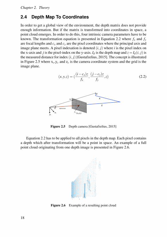
In order to get a global view of the environment, the depth matrix does not provideenough information. But if the matrix is transformed into coordinates in space, apoint cloud emerges. In order to do this, four intrinsic camera parameters have to beknown. The transformation equation is presented in Equation 2.2 where fx and fyare focal lengths and cx and cy are the pixel coordinates where the principal axis andimage plane meets. A pixel indexation is denoted (i, j) where i is the pixel index onthe x-axis and j is the pixel-index on the y-axis. Id is the depth map and z= Id(i, j) isthe measured distance for index (i, j) [Gustafzelius, 2015]. The concept is illustratedin Figure 2.5 where xc,yc and zc is the camera coordinate system and the grid is theimage plane.

(x,y,z) = ((i� cx)z

fx,( j� cy)z

fy,z) (2.2)

z

x

y

(cx,cy)

(i,j)

optical axiszc

xc

yc

Figure 2.5 Depth camera [Gustafzelius, 2015]

Equation 2.2 has to be applied to all pixels in the depth map. Each pixel containsa depth which after transformation will be a point in space. An example of a fullpoint cloud originating from one depth image is presented in Figure 2.6.

Figure 2.6 Example of a resulting point cloud

18

2.5 Random Sample Consensus (RANSAC)

2.5 Random Sample Consensus (RANSAC)

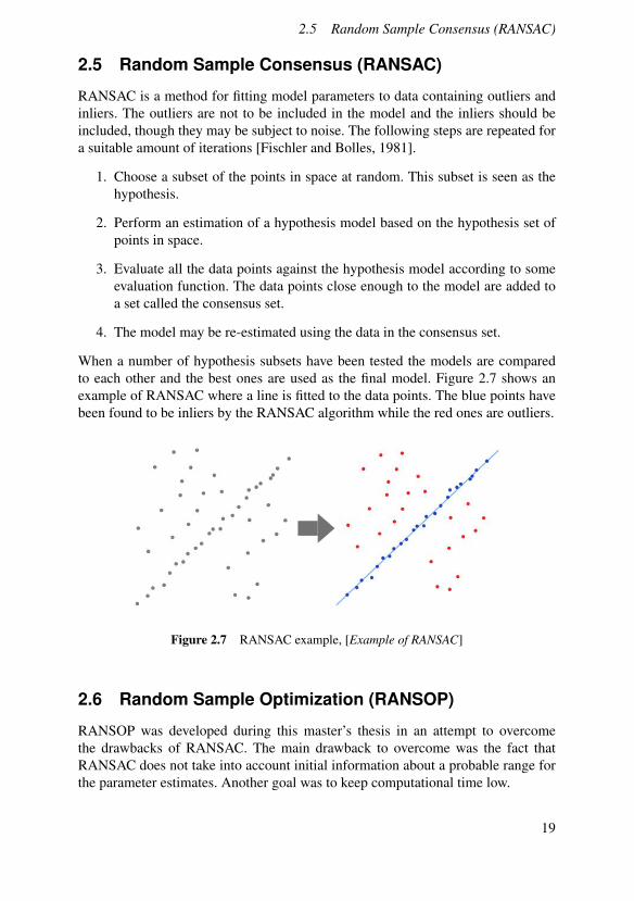
RANSAC is a method for fitting model parameters to data containing outliers andinliers. The outliers are not to be included in the model and the inliers should beincluded, though they may be subject to noise. The following steps are repeated fora suitable amount of iterations [Fischler and Bolles, 1981].

1. Choose a subset of the points in space at random. This subset is seen as thehypothesis.

2. Perform an estimation of a hypothesis model based on the hypothesis set ofpoints in space.

3. Evaluate all the data points against the hypothesis model according to someevaluation function. The data points close enough to the model are added toa set called the consensus set.

4. The model may be re-estimated using the data in the consensus set.

When a number of hypothesis subsets have been tested the models are comparedto each other and the best ones are used as the final model. Figure 2.7 shows anexample of RANSAC where a line is fitted to the data points. The blue points havebeen found to be inliers by the RANSAC algorithm while the red ones are outliers.

Figure 2.7 RANSAC example, [Example of RANSAC]

2.6 Random Sample Optimization (RANSOP)

RANSOP was developed during this master’s thesis in an attempt to overcomethe drawbacks of RANSAC. The main drawback to overcome was the fact thatRANSAC does not take into account initial information about a probable range forthe parameter estimates. Another goal was to keep computational time low.

19

Chapter 2. Theory

The standard RANSAC assumes that there is no information about the modelin addition to the data points and model structure. But using the RANSOP insteadof the standard RANSAC comes at the cost of robustness. There are no guaranteesthat RANSOP will find the correct plane and there is always the risk of statisticalvariance in the chosen points to throw the results off.

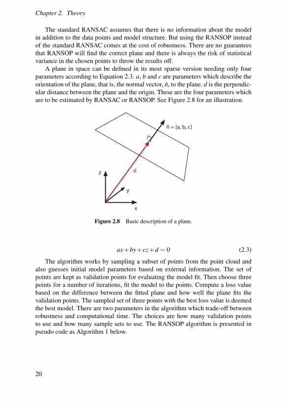
A plane in space can be defined in its most sparse version needing only fourparameters according to Equation 2.3. a, b and c are parameters which describe theorientation of the plane, that is, the normal vector, n̄, to the plane. d is the perpendic-ular distance between the plane and the origin. These are the four parameters whichare to be estimated by RANSAC or RANSOP. See Figure 2.8 for an illustration.

d

n = [a, b, c]

x

z

y

Figure 2.8 Basic description of a plane.

ax+by+ cz+d = 0 (2.3)

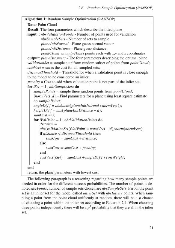
The algorithm works by sampling a subset of points from the point cloud andalso guesses initial model parameters based on external information. The set ofpoints are kept as validation points for evaluating the model fit. Then choose threepoints for a number of iterations, fit the model to the points. Compute a loss valuebased on the difference between the fitted plane and how well the plane fits thevalidation points. The sampled set of three points with the best loss value is deemedthe best model. There are two parameters in the algorithm which trade-off betweenrobustness and computational time. The choices are how many validation pointsto use and how many sample sets to use. The RANSOP algorithm is presented inpseudo code as Algorithm 1 below.

20

2.6 Random Sample Optimization (RANSOP)

Algorithm 1: Random Sample Optimization (RANSOP)Data: Point CloudResult: The four parameters which describe the fitted planeinput : nbrValidationPoints - Number of points used for validation

nbrSampleSets - Number of sets to sampleplaneInitNormal - Plane guess normal vectorplaneInitDistance - Plane guess distancepointCloud with nbrPoints points each with x,y and z coordinates

output: planeParamers - The four parameters describing the optimal planevalidationSet = sample a uniform random subset of points from pointCloud;costVect = saves the cost for all sampled sets;distanceT hreshold = Threshold for when a validation point is close enoughto the model to be considered an inlier;penalty = Cost to add when validation point is not part of the inlier set;for iSet = 1 : nbrSampleSets do

samplePoints = sample three random points from pointCloud;[normVect,d] = Find parameters for a plane using least square estimateon samplePoints;angleDi f f = abs(acos(planeInitNormal ⇤normVect));heightDi f f = abs(planeInitDistance�d);sumCost = 0;for iValPoint = 1 : nbrValidationPoints do

distance =abs(validationSet(iValPoint)⇤normVect �d)/norm(normVect);if distance < distanceT hreshold then

sumCost = sumCost +distance;else

sumCost = sumCost + penalty;endcostVect(iSet) = sumCost +angleDi f f ⇤ costWeight;

endendreturn: the plane parameters with lowest cost

The following paragraph is a reasoning regarding how many sample points areneeded in order for the different success probabilities. The number of points is de-noted nbrPoints, number of sample sets chosen are nbrSampleSets. Part of the pointset is an inlier set for the model called inlierSet with nbrInliers points. When sam-pling a point from the point cloud uniformly at random, there will be a p chanceof choosing a point within the inlier set according to Equation 2.4. When choosingthree points independently there will be a p3 probability that they are all in the inlierset.

21

Chapter 2. Theory

P(point 2 inlierSet) =nbrInliersnbrPoints

= p (2.4)

The binomial distribution can be used to find the probabilities of successfullysampling three inlier points for different values of nbrSampleSets. The value of thebinomial random variable is the number of “successes” out of a random sample of ntrials. nbrSampleSets equals the number of trials and p is the probability of successfor one trial, which equals p3. The binomial probability formula is presented inEquation 2.5 where y is the number of successful trials. One success is enough inorder for RANSOP to produce a working model, so finding the probabilities forP(y � 1) is of importance for analyzing how many sets to be sampled.

P(y successes in n trials) =n!

y!(n� y)!py(1�p)n�y (2.5)

2.7 Planning Problem Formulation

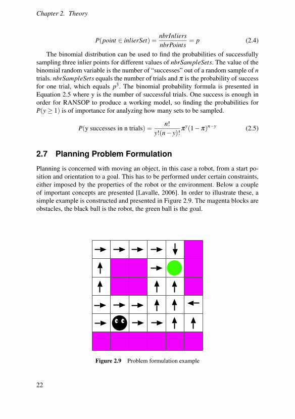
Planning is concerned with moving an object, in this case a robot, from a start po-sition and orientation to a goal. This has to be performed under certain constraints,either imposed by the properties of the robot or the environment. Below a coupleof important concepts are presented [Lavalle, 2006]. In order to illustrate these, asimple example is constructed and presented in Figure 2.9. The magenta blocks areobstacles, the black ball is the robot, the green ball is the goal.

Figure 2.9 Problem formulation example

22

2.8 Non-holonomic System

States The states are all possible situations in a planning problem. There couldbe a finite number of states in a discretized environment or an infinite number ofstates in a continuous environment. In the simple example above all white cells arepossible states for the robot.

Configuration Space (C-space) The configuration space of a robot is a set of allpossible states. C-free is the part of configuration space not occupied by an obstacle.In the simple example the c-space is the whole grid while c-free is the set of whitecells, which are traversable.

Time Time always has to be taken into account. Either as an objective variable foroptimizing the planning, or as a way of keeping a sequence in order.

Actions An action can be performed by the robot in order to change the state. Theset of actions in the simple example is to move right, left, up or down.

Plan A plan is a strategy for determining which actions to take in every statesin order to reach a goal state. The current plan in the simple example is illustratedby the arrows. There is an action associated with each possible state, that is, thepreferred direction to walk in every cell is the direction of the arrows. The set of allof these actions constitutes a plan.

2.8 Non-holonomic System

A non-holonomic system is where the current state depends on the path which wastaken to reach the state. It is described by a set of parameters subject to differentialconstraints, such that if a system evolves along a path in the c-space and then returnsto the original set of values the system itself might not have returned to the originalstate [Lavalle, 2006].

2.9 Motion Planning

The motion planning problem consists of building an algorithm to be given a high-level specification of a task and converting it to low-level instructions. It has to bepossible for an autonomous system to actuate the instructions. Motion planning isusually only concerned with the issue of kinematics and velocities, but does notregard dynamics and differential constraints. It is usually performed in a continuousworld and the objective is to find a path from start to goal state in the free c-spacewithout colliding with obstacles [Lavalle, 2006].

2.10 Overview of Planning in Continuous Space

The state space in the real world is uncountable infinite and a robot motion plan-ning problem must therefore be simplified in some way. Configuration space is the

23

Chapter 2. Theory

state space in motion planning. The number of dimensions of c-space correspondsto the number of degrees of freedom of the robot. Using the configuration space,motion planning will be viewed as a kind of search in a high-dimensional config-uration space that contains implicitly represented obstacles. There are two waysof discretizing the c-space, combinatorial and sampling based [Lavalle, 2006]. Amajority of planning methods contains two steps: Building the road map and per-forming search in the road map graph.

2.11 Road Map

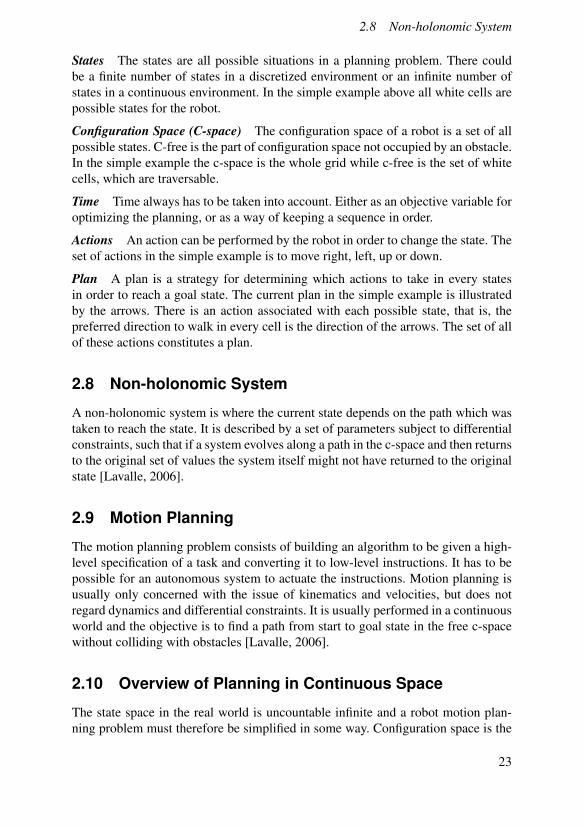
A road map is a graph of connections between possible states, essentially the topol-ogy of a planning problem. A road map is usually the result of a discretization ofthe continuous c-space. In the graph each vertex is a state, while the edges denotepossible transitions between the states, that is, a collision free path. For many of theplanning methods presented, one of the first steps is to build a road map. An ex-ample is presented in Figure 2.10. The free space is filled with possible discretizedstates displayed as the blue graph network. The magenta obstacles can not be tra-versed and are therefore not connected in the graph. Note that this is a simple twodegree-of-freedom example where the state space and road map can be visualizedin a simple way.

Figure 2.10 Road map graph example

24

2.11 Road Map

Combinatorial PlanningCombinatorial planning characterizes free c-space explicitly by capturing the con-nectivity of free c-space in a graph. These methods have a couple of convenientfeatures. They are complete, which means that if a solution exists it will be found,even though it might be time consuming. The solution is found by using search anda failure will be reported if no path exists. All of these methods produce a road map.

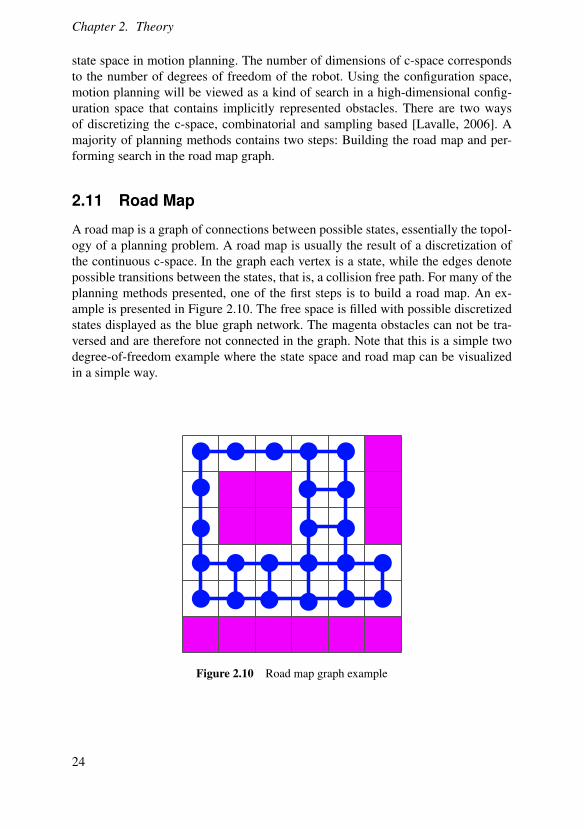
Uniform Grid Discretization This method of building a road map is one of themost straight forward. The whole space is discretized into a uniform grid. Cells aremarked as either blocked or free. The free configuration space is discretized as freecells and these cells are put as vertices in the road map graph. They are connectedwith edges in order to create the map. The vertices can be connected in differentways. One option is to connect a vertex only to the four adjoining neighbors [Russeland Norvig, 2010]. Another method is to connect to the eight adjoining neighborsand thereby allowing diagonal movement in the path. Figure 2.11 provides an ex-ample where the first image is the continuous world with the pink obstacles. Imagetwo contains the uniformly discretized map with the road map graph in blue.

Figure 2.11 Uniform grid discretization example

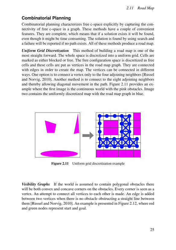
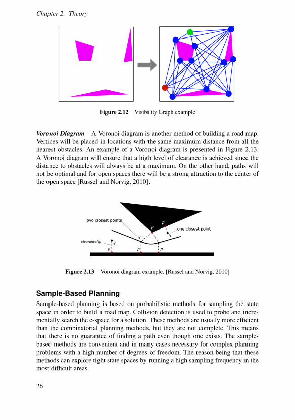
Visibility Graphs If the world is assumed to contain polygonal obstacles therewill be both convex and concave corners on the obstacles. Every corner is seen as avertex. An attempt to connect all vertices to each other is made. An edge is addedbetween two vertices when there is no obstacle obstructing a straight line betweenthem [Russel and Norvig, 2010]. An example is presented in Figure 2.12, where redand green nodes represent start and goal.

25

Chapter 2. Theory

Figure 2.12 Visibility Graph example

Voronoi Diagram A Voronoi diagram is another method of building a road map.Vertices will be placed in locations with the same maximum distance from all thenearest obstacles. An example of a Voronoi diagram is presented in Figure 2.13.A Voronoi diagram will ensure that a high level of clearance is achieved since thedistance to obstacles will always be at a maximum. On the other hand, paths willnot be optimal and for open spaces there will be a strong attraction to the center ofthe open space [Russel and Norvig, 2010].

Figure 2.13 Voronoi diagram example, [Russel and Norvig, 2010]

Sample-Based PlanningSample-based planning is based on probabilistic methods for sampling the statespace in order to build a road map. Collision detection is used to probe and incre-mentally search the c-space for a solution. These methods are usually more efficientthan the combinatorial planning methods, but they are not complete. This meansthat there is no guarantee of finding a path even though one exists. The sample-based methods are convenient and in many cases necessary for complex planningproblems with a high number of degrees of freedom. The reason being that thesemethods can explore tight state spaces by running a high sampling frequency in themost difficult areas.

26

2.11 Road Map

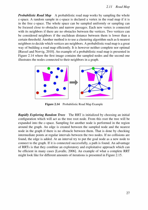
Probabilistic Road Map A probabilistic road map works by sampling the wholec-space. A random sample in c-space is declared a vertex in the road map if it isin the free c-space. The whole space can be sampled uniformly or sampling canbe focused close to obstacles and narrow passages. Each new vertex is connectedwith its neighbors if there are no obstacles between the vertices. Two vertices canbe considered neighbors if the euclidean distance between them is lower than acertain threshold. Another method is to use a clustering algorithm such as k-nearestneighbors to decide which vertices are neighbors. A probabilistic road map is a greatway of building a road map efficiently. It is however neither complete nor optimal[Russel and Norvig, 2010]. An example of a probabilistic road map is presented inFigure 2.14 where the first image contains the sampled nodes and the second oneillustrates the nodes connected to their neighbors in a graph.

Figure 2.14 Probabilistic Road Map Example

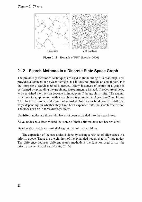
Rapidly Exploring Random Trees The RRT is initialized by choosing an initialconfiguration which will act as the tree root node. From this root the tree will beexpanded into the c-space. Sampling for another node is performed in the regionaround the graph. An edge is created between the sampled node and the nearestnode in the graph if there is no obstacle between them. That is done by checkingintermediate points at regular intervals between the two nodes. If no collisions arefound, the edge is added. At an interval try to put the goal node as a new node toconnect to the graph. If it is connected successfully, a path is found. An advantageof RRTs is that they combine an exploratory and exploitative approach which canbe efficient in many cases [Lavalle, 2006]. An example of what a complete RRTmight look like for different amounts of iterations is presented in Figure 2.15.

27

Chapter 2. Theory

Figure 2.15 Example of RRT, [Lavalle, 2006]

2.12 Search Methods in a Discrete State Space Graph

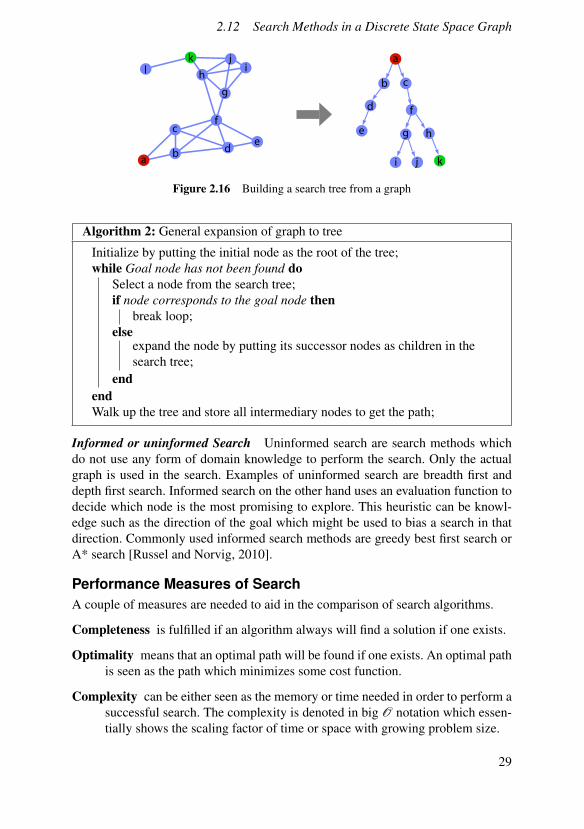
The previously mentioned techniques are used in the building of a road map. Thisprovides a connection between vertices, but it does not provide an actual path. Forthat purpose a search method is needed. Many instances of search in a graph isperformed by expanding the graph into a tree structure instead. If nodes are allowedto be revisited the tree can become infinite, even if the graph is finite. The generalstructure of a graph search with a search tree is presented in Algorithm 2 and Figure2.16. In this example nodes are not revisited. Nodes can be denoted in differentways depending on whether they have been expanded into the search tree or not.The nodes can be in three different states.

Unvisited nodes are those who have not been expanded into the search tree.

Alive nodes have been visited, but some of their children have not been visited.

Dead nodes have been visited along with all of their children.

The expansion of the tree nodes is done by storing a new set of alive states in apriority queue. These are the children of the expanded nodes, that is, fringe nodes.The difference between different search methods is the function used to sort thepriority queue [Russel and Norvig, 2010].

28

2.12 Search Methods in a Discrete State Space Graph

a

a

b

b

c

c

d

d

ee

ff

g

g

h

h

i

i

j

j

k

k

l

Figure 2.16 Building a search tree from a graph

Algorithm 2: General expansion of graph to tree

Initialize by putting the initial node as the root of the tree;while Goal node has not been found do

Select a node from the search tree;if node corresponds to the goal node then

break loop;else

expand the node by putting its successor nodes as children in thesearch tree;

endendWalk up the tree and store all intermediary nodes to get the path;

Informed or uninformed Search Uninformed search are search methods whichdo not use any form of domain knowledge to perform the search. Only the actualgraph is used in the search. Examples of uninformed search are breadth first anddepth first search. Informed search on the other hand uses an evaluation function todecide which node is the most promising to explore. This heuristic can be knowl-edge such as the direction of the goal which might be used to bias a search in thatdirection. Commonly used informed search methods are greedy best first search orA* search [Russel and Norvig, 2010].

Performance Measures of SearchA couple of measures are needed to aid in the comparison of search algorithms.

Completeness is fulfilled if an algorithm always will find a solution if one exists.

Optimality means that an optimal path will be found if one exists. An optimal pathis seen as the path which minimizes some cost function.

Complexity can be either seen as the memory or time needed in order to perform asuccessful search. The complexity is denoted in big O notation which essen-tially shows the scaling factor of time or space with growing problem size.

29

Chapter 2. Theory

Branching factor, b is the number of children each node has.

Goal depth, d is the depth of the shallowest goal node, that is, the number of stepsin the search tree from the start node to the closest goal node.

Max depth, m is the maximum depth of any node in the tree.

Breadth First SearchBreadth first search (BFS) will explore the graph by only expanding deeper into thegraph when all of the nodes at the same level in the search tree has been expanded.In BFS the fringe nodes are kept in a FIFO, first in first out, queue [Russel andNorvig, 2010].

Completeness Yes, if the branching factor, b, is finite

Optimality If the cost function is the number of steps in the graph, then yes.

Complexity O(bd) is the complexity for both time and space.

Depth First SearchDFS is the opposite of BFS and performs a search along one branch of the tree untilit can not be expanded any more. The fringe node expanded is the most recentlyinserted into the tree. Fringe nodes are kept in a LIFO, last in first out, queue [Russeland Norvig, 2010].

Completeness Yes, if m is finite and there are no loops in the state graph or if statesare not revisited.

Optimality No

Complexity O(bm) is the complexity for time, while O(bm) is the space complex-ity.

Uniform Cost SearchBFS and DFS only use the topology of the graph in order to find a path. If a costcan be estimated for traversal of each edge, this information can be used in order tofind a more optimal path faster. Uniform cost search uses a priority queue to storethe fringe nodes where the priority is decided by total distance from root to node.The distances of the edges are added and the shortest total distance will have thehighest priority and be expanded next [Russel and Norvig, 2010].

Completeness Yes, if b is finite and all edges have a cost larger than 0.

Optimality Yes

Complexity O(b1+ f loor(Ce )) is both the time and space complexity, where C is the

cost of the optimal solution and e the smallest possible edge cost.

30

2.12 Search Methods in a Discrete State Space Graph

A* SearchA* is similar to uniform cost search but in addition to using the cost for traverseddistance along the edges a heuristic is used to estimate the distance to goal.

n: The current node

g(n): Cost from root to node n.

h(n): Estimated cost from node n to goal.

f(n) = g(n) + h(n): Total cost.

The node with the lowest f(n) will have the highest priority in the priority queue andwill therefore be expanded first.

Completeness Yes, if all edges have a cost larger than zero.

Optimality Yes, if the heuristic is admissible.

Complexity Depends on which heuristic is used.

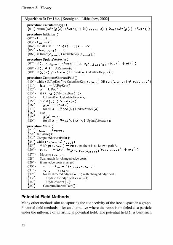
D* SearchA drawback of the previously mentioned search methods is that if there is a changein the planning map, position of the robot or goal, the whole search has to be re-performed. D* is short for dynamic A* and is a version of A* but with a minimum ofrecalculations for a changing environment. When the environment changes, D* onlyre-plans the path locally. D* Lite is another implementation of the D* algorithmand is at least as efficient. That makes D* Lite well suited for real-time application[Koenig and Likhachev, 2002]. The algorithm is presented in Algorithm 3.

31

Chapter 2. Theory

Algorithm 3: D* Lite, [Koenig and Likhachev, 2002]procedure CalculateKey01’ return ;

procedure Initialize02’ ;03’04’ for all ;05’ ;06’ U.Insert CalculateKey ;

procedure UpdateVertex07’ if ;

08’ if U.Remove ;09’ if U.Insert CalculateKey ;

procedure ComputeShortestPath10’ while U.TopKey CalculateKey OR11’ U.TopKey12’ U.Pop ;13’ if CalculateKey14’ U.Insert CalculateKey15’ else if16’ ;17’ for all UpdateVertex ;18’ else19’ ;20’ for all UpdateVertex ;

procedure Main21’22’ Initialize ;23’ ComputeShortestPath ;24’ while25’ /* if then there is no known path */26’ ;

27’ Move to ;28’ Scan graph for changed edge costs;29’ if any edge costs changed30’31’32’ for all directed edges with changed edge costs33’ Update the edge cost ;34’ UpdateVertex ;35’ ComputeShortestPath ;

Potential Field MethodsMany other methods aim at capturing the connectivity of the free c-space in a graph.Potential field methods offer an alternative where the robot is modeled as a particleunder the influence of an artificial potential field. The potential field U is built such

32

2.12 Search Methods in a Discrete State Space Graph

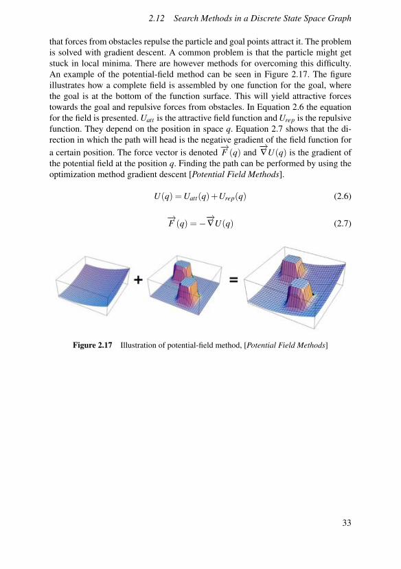
that forces from obstacles repulse the particle and goal points attract it. The problemis solved with gradient descent. A common problem is that the particle might getstuck in local minima. There are however methods for overcoming this difficulty.An example of the potential-field method can be seen in Figure 2.17. The figureillustrates how a complete field is assembled by one function for the goal, wherethe goal is at the bottom of the function surface. This will yield attractive forcestowards the goal and repulsive forces from obstacles. In Equation 2.6 the equationfor the field is presented. Uatt is the attractive field function and Urep is the repulsivefunction. They depend on the position in space q. Equation 2.7 shows that the di-rection in which the path will head is the negative gradient of the field function fora certain position. The force vector is denoted

�!F (q) and

�!—U(q) is the gradient of

the potential field at the position q. Finding the path can be performed by using theoptimization method gradient descent [Potential Field Methods].

U(q) =Uatt(q)+Urep(q) (2.6)

�!F (q) =�

�!—U(q) (2.7)

Figure 2.17 Illustration of potential-field method, [Potential Field Methods]

33

3

Method

This chapter includes comparisons between various theories, methods and hardwaretogether with a small discussion on why certain programs, sensors and tools wereused. Implementations of suitable methods and theories from Chapter 2 are alsodescribed.

First the software used are described and discussed, followed by the mappingsensors, an overview of the mode used for autonomous walk and a discussion of thesampling frequency. Thereafter positioning, mapping, planning and search prob-lems of the hexapod are investigated and solved. Lastly, the changes of the remotecontrol, the terrain handling problem and changes of the electrical assembly aredescribed.

3.1 Simulink Model

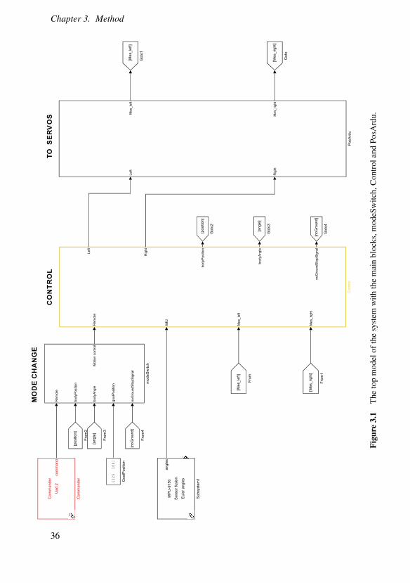
The Simulink model developed in this project has its origin in the previous thesisby Dan Thilderkvist and Sebastian Svensson. It consists of three main blocks calledmodeSwitch, Control and PosArdu. Figure 3.1 shows the top layer of the Simulinkmodel and the connection between the three main blocks. ModeSwitch decideswhen to switch mode and what should be done when a mode switches. This meansthat the camera S-function, the planning algorithms and the movement changes ofthe sensor mode are all included in this block. The output of the modeSwitch blockis the new movement signal. More on the different parts of modeSwitch are ex-plained below. The control block contains the locomotion controls which includeswhich leg to move, how it should be moved and how the rest of the body shouldfollow. This is for example where the force sensors have been integrated. A lot ofthe changes since the last master’s thesis have been done in the subblock calledTrajectorySystem in MainControllerNew. The TrajectorySystem block creates thedifferent positions for the leg trajectory and therefore this also contains the extendedtrajectory showed in Chapter 3. From the control block the different positions aresent to the third main block, called PosArdu and the mission of this block is to takethe leg positions and forward them to the servos. The function and construction of

34

3.1 Simulink Model

the control block and the PosArdu block are explained in more detail in the previ-ous master’s thesis by Dan Thilderkvist and Sebastian Svensson [Thilderkvist andSvensson, 2015].

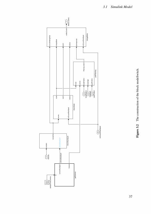
modeSwitchThe block modeSwitch is, as mentioned previously, the block where mode changesare made. As can be seen in Figure 3.2, it consists of five sub-blocks called get-Camera, checkStopSignal, checkMode, pathPlanning and finally changeMode. Theinputs are the signal from the remote control, position and angle of the hexapod,goal position of the path-planning and a signal called noGroundStopSignal.

NoGroundStopSignal is used in mode 3, sensor mode, to check whether theactive foot has ground contact at the end of the trajectory. If the sensors do notregister any pressure the noGroundStopSignal becomes true and the movement isreversed.

getCamera The block getCamera basically gets the information from the cameraand sends this information to the path planning block where this information ishandled. The other output from the getCamera block is used in mode 2 where therobot is moving straight forward until the camera registers an obstacle in front ofthe camera. This signal simply becomes 1 if there is an obstacle and 0 if the spaceis clear.

checkStopSignal The only thing this block does is to change mode to mode 4 ifthe robot is in mode 2 and if the stop signal from the previous block is 1.

checkMode This block uses the information from the buttons to check whichmode is active. It also checks the signal called noGroundStopSignal to see if thesensors have indicated ground contact. This is only done in mode 3. Output fromthe checkMode block is the active mode and it is thereafter used to activate the path-planning algorithm, if the mode is 5, or to tell the final block to change the origin ofthe movements.

pathPlanning The pathPlanning block takes the information from the camera tomake a map of the world, it uses the position and angle of the hexapod to decidewhere in the room the robot is at the moment, it looks at the input goalPositionto decide where the robot should move and it checks which mode the robot is in.Since the path-planning calculations together with the mapping is demanding it ispreferred to only perform these calculations while in mode 5, planning mode.

changeMode The last sub-block in the switchMode block is used to actuallychange the mode. After this block the rest of the model gets information about howit should move. For example, if mode 1 is active, the information about the move-ment should be taken from the remote control but if mode 2, the camera mode,is active the movement should just be straight forward or stop, depending on thecamera stop signal.

35

Chapter 3. Method

CO

NTR

OL

TO S

ER

VO

S

MO

DE

CH

AN

GE

Left

Rig

ht

Mes

_lef

t

Mes

_rig

ht

PosA

rdu

Rem

ote

body

Posi

tion

body

Angl

e

goal

Posi

tion

noG

roun

dSto

pSig

nal

Mot

ion

cont

rol

mod

eSw

itch

Com

man

der

Uar

t 2co

mm

and

Com

man

der

[125

100]

Goa

lPos

ition

[Mes

_rig

ht]

Got

o

[Mes

_lef

t]

Got

o1

[Mes

_lef

t]

From

[Mes

_rig

ht]

From

1

Rem

ote

IMU

Mes

_lef

t

Mes

_rig

ht

Left

Rig

ht

body

Posi

tion

body

Angl

e

noG

roun

dSto

pSig

nal

Con

trol

[pos

ition]

Got

o2

[pos

ition]

From

2

[ang

le]

From

3

[ang

le]

Got

o3

[noG

roun

d]

Got

o4

[noG

roun

d]

From

4

MP

U-9

150

Sen

sor f

usio

n

Eul

er a

ngle

s

angl

es

Subs

yste

m1

Figu

re3.

1Th

eto

pm

odel

ofth

esy

stem

with

the

mai

nbl

ocks

,mod

eSw

itch,

Con

trola

ndPo

sArd

u.

36

3.1 Simulink Model

1

Rem

ote

1

Motion c

ontr

ol

rem

ote

In

Cam

era

Sto

pS

ignal

rem

ote

Out

checkS

top

Sig

nal

rem

ote

no

Gro

und

Sto

pS

ignal

mode

lookV

buttons

checkM

ode

2

bodyP

ositio

n

3

bodyA

ngle

4

goalP

ositio

n

sam

ple

Tim

eC

am

era

cam

era

Sto

pS

ignal

Cam

era

getC

am

era

norm

alW

alk

ing

Mode

change

Mode

lookV

buttons

pla

nnin

gm

ode

no

Gro

und

Sto

pS

ignalm

otio

nC

ontr

ol

change

Mode

mode

cam

era

bodyP

ositi

on

bodyA

ngle

goalP

ositi

on

Pla

nnin

g m

ode 5

path

Pla

nnin

g

5

no

Gro

und

Sto

pS

ignal

cam

era

Sto

pS

ignal

Figu

re3.

2Th

eco

nstru

ctio

nof

the

bloc

km

odeS

witc

h.

37

Chapter 3. Method

3.2 Friction Modeling in SimMechanics

A model of the robot was set up in SimMechanics according to Thilderkvist andSvensson [Thilderkvist and Svensson, 2015]. This model contained all mechani-cal parts of the robot complete with joints and the control system could be run onthe model. However this could only verify the mechanical system isolated froman external world. Since a goal of this thesis was to navigate in an environmentwith obstacles and terrain another method or software had to be used. A first stepwas to improve the SimMechanic model with contact and friction forces betweenthe feet of the hexapod and the ground. Since there was poor support for contactforces and friction in the native SimMechanics toolboxes an external package wasused [SimScape Multibody Contact Forces Library]. The toolbox allowed for fric-tion and contact force model blocks to be set up between the floor and the feet. Thisallowed for the Hexapod model to walk around on a flat surface.

3.3 Choice of Simulation Software

Since the solutions for modeling interactions between the robot and environmentwas cumbersome in SimMechanics, other alternatives for simulating robots wereresearched. Gazebo, MuJoCo, V-REP and Webots are all popular programs for sim-ulating multi-body dynamics, force contacts and friction through their physic en-gines. Having support for CAD-parts and capabilities for simulating a virtual time-of-flight camera were also important features. They all have similar capabilities andeither one of the programs seemed to work for our purposes. Since code generationto the hardware is performed from the Simulink environment simulink also had tobe used when running simulations. None of the simulation programs had an API forSimulink connection, but they all had different types of Matlab API’s. In the end wechose to go with V-REP because of its convenient Matlab API and free academiclicense.

3.4 Setting Up the Hexapod in V-REP

All of the individual parts of the Hexapod were provided in the form of CAD-models. These had to be converted into STL file format in order for them to beimportable into V-REP. This meant that all parts of the hexapod had the correctweights and moment of inertia. The parts were also dynamically enabled in orderfor simulations to include collisions, falls and for gravity to act upon the parts. Allparts were also enabled for sensor interaction and camera rendering so they couldbe captured by the depth-camera. The robot contains 18 leg parts and one solidbody part. All of the parts were assembled with joints according to Thilderkvist andSvensson [Thilderkvist and Svensson, 2015].

38

3.4 Setting Up the Hexapod in V-REP

Virtual Depth CameraV-REP includes virtual sensors so the depth-camera can be simulated and send adepth matrix back to Matlab. Thereby the information between V-REP and Matlabwill replicate the information which is to be sent between the BeagleBone and thecamera. The resolution of the real camera used is 320x240 but unfortunately V-REPonly supports 1:1 aspect ratios, therefore 240x240 was used in V-REP. The field ofview and focal lengths of the real camera was used with the virtual one. The camerawas mounted and the final V-REP assembly of the hexapod is presented in Figure3.3.

Figure 3.3 Assembled hexapod in V-REP

Modeling Dynamic Behavior in V-REPStatic shapes will not be influenced by gravity or dynamically enabled joints, whiledynamic shapes will. Respondable shapes will be affected by other respondableshapes in collision. The computations of dynamic and respondable parts are heavy,primitive shapes were therefore created to represent the complete CAD-parts. Alldynamic and collision computations are performed on the simple parts while theoriginal parts are used in the rendering of the visualization. The tibia parts of thelegs are first selected and a convex hull shape created. This shape is to be used in thecollision computations. It is connected to the corresponding part and collision masksare set so there will be no collisions between connected parts of the leg [Designingdynamic simulations].

39

Chapter 3. Method

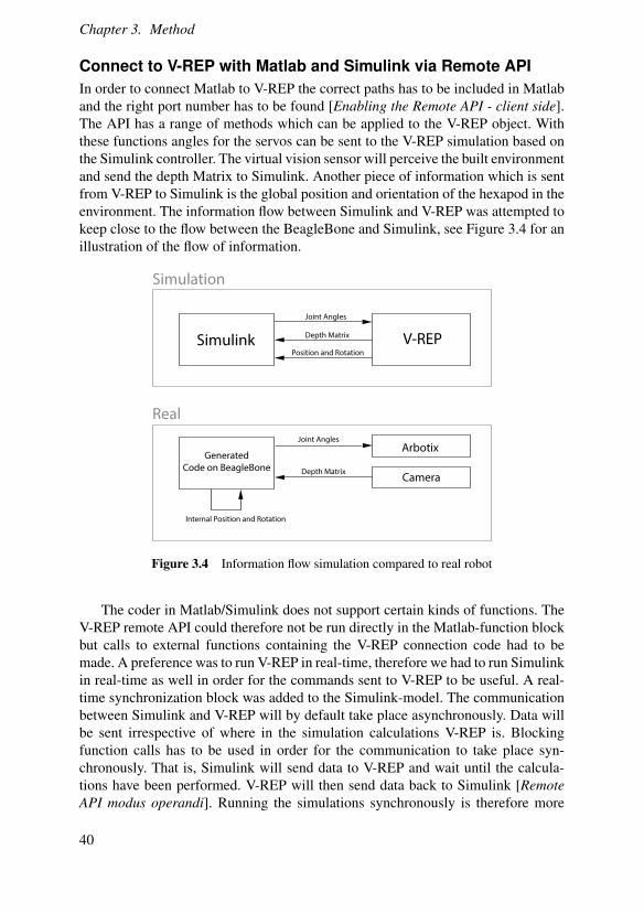
Connect to V-REP with Matlab and Simulink via Remote APIIn order to connect Matlab to V-REP the correct paths has to be included in Matlaband the right port number has to be found [Enabling the Remote API - client side].The API has a range of methods which can be applied to the V-REP object. Withthese functions angles for the servos can be sent to the V-REP simulation based onthe Simulink controller. The virtual vision sensor will perceive the built environmentand send the depth Matrix to Simulink. Another piece of information which is sentfrom V-REP to Simulink is the global position and orientation of the hexapod in theenvironment. The information flow between Simulink and V-REP was attempted tokeep close to the flow between the BeagleBone and Simulink, see Figure 3.4 for anillustration of the flow of information.

Simulink

GeneratedCode on BeagleBone

V-REP

Arbotix

Camera

Simulation

Real

Joint Angles

Joint Angles

Depth Matrix

Depth Matrix

Position and Rotation

Internal Position and Rotation

Figure 3.4 Information flow simulation compared to real robot

The coder in Matlab/Simulink does not support certain kinds of functions. TheV-REP remote API could therefore not be run directly in the Matlab-function blockbut calls to external functions containing the V-REP connection code had to bemade. A preference was to run V-REP in real-time, therefore we had to run Simulinkin real-time as well in order for the commands sent to V-REP to be useful. A real-time synchronization block was added to the Simulink-model. The communicationbetween Simulink and V-REP will by default take place asynchronously. Data willbe sent irrespective of where in the simulation calculations V-REP is. Blockingfunction calls has to be used in order for the communication to take place syn-chronously. That is, Simulink will send data to V-REP and wait until the calcula-tions have been performed. V-REP will then send data back to Simulink [RemoteAPI modus operandi]. Running the simulations synchronously is therefore more

40

3.5 Mapping sensors

time consuming. It can be important to use synchronous execution when dynamicsare of importance. In this case it was preferred to have faster execution.

Servo Joint ControllersMovement of the hexapod is performed by controlling the joints of the servos. Onthe real robot an angle value is sent to the servos and an internal PID controllermoves the joints [Thilderkvist and Svensson, 2015]. The same behavior is prefer-able in the virtual simulation environment in order for the main controller to sendthe same information in both the real case and the virtual. Luckily V-REP has built-in PID controllers in the joint objects which were to be used for this purpose. Themaximum torques are 16.5 kgcm for the real servos, and the virtual torque limitwas therefore set to the same. Since the real servo PID parameters were unknownthe virtual PID parameters were found by trying to compare the behavior in simula-tion with the real behavior. The real servos never had any difficulties following thecreated trajectories. The PID controller in simulation was therefore tuned to alsofollow the trajectories.

3.5 Mapping sensors

In order for the robot to navigate autonomously in the world, some sort of mappingsensor is necessary. There is a myriad of sensors which can be used to perceive theenvironment but a Time-of-Flight camera was eventually used for convenience.

Time-of-Flight CameraThe TOF camera chosen in this project is an Asus Xtion Pro Live. It features amongother things an infrared (IR) emitter and detector that captures the depth image andit features a RGB camera. The two different features are separated in two matri-ces when delivered. It is small and light weighted and therefor works fine on thehexapod [Xtion PRO LIVE].

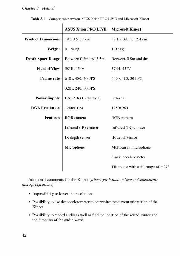
Another 3D sensing camera considered was Microsoft’s Kinect for Windows.The two cameras are much alike but some of the differences are explained in Table3.1.

41

Chapter 3. Method

Table 3.1 Comparison between ASUS Xtion PRO LIVE and Microsoft Kinect

ASUS Xtion PRO LIVE Microsoft Kinect

Product Dimensions 18 x 3.5 x 5 cm 38.1 x 38.1 x 12.4 cm

Weight 0.170 kg 1.09 kg

Depth Space Range Between 0.8m and 3.5m Between 0.8m and 4m

Field of View 58°H, 45°V 57°H, 43°V

Frame rate 640 x 480: 30 FPS 640 x 480: 30 FPS

320 x 240: 60 FPS

Power Supply USB2.0/3.0 interface External

RGB Resulution 1280x1024 1280x960

Features RGB camera RGB camera

Infrared (IR) emitter Infrared (IR) emitter

IR depth sensor IR depth sensor

Microphone Multi-array microphone

3-axis accelerometer

Tilt motor with a tilt range of ±27°.

Additional comments for the Kinect [Kinect for Windows Sensor Componentsand Specifications]:

• Impossibility to lower the resolution.

• Possibility to use the accelerometer to determine the current orientation of theKinect.

• Possibility to record audio as well as find the location of the sound source andthe direction of the audio wave.

42

3.6 Camera Implementation

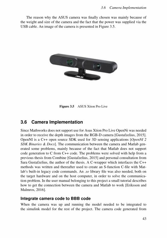
The reason why the ASUS camera was finally chosen was mainly because ofthe weight and size of the camera and the fact that the power was supplied via theUSB cable. An image of the camera is presented in Figure 3.5.

Figure 3.5 ASUS Xtion Pro Live

3.6 Camera Implementation

Since Mathworks does not support use for Asus Xtion Pro Live OpenNi was neededin order to receive the depth images from the RGB-D camera [Gustafzelius, 2015].OpenNI is a C++ open source SDK used for 3D sensing applications [OpenNI 2SDK Binaries & Docs]. The communication between the camera and Matlab gen-erated some problems, mainly because of the fact that Matlab does not supportcode generation to C from C++ code. The problems were solved with help from aprevious thesis from Combine [Gustafzelius, 2015] and personal consultation fromSara Gustafzelius, the author of the thesis. A C-wrapper which interfaces the C++methods was written and thereafter used to create an S-function C-file with Mat-lab’s built-in legacy code commands. An .so library file was also needed, both onthe target hardware and on the host computer, in order to solve the communica-tion problem. In the user manual belonging to this project a small tutorial describeshow to get the connection between the camera and Matlab to work [Eriksson andMalmros, 2016].

Integrate camera code to BBB codeWhen the camera was up and running the model needed to be integrated tothe simulink model for the rest of the project. The camera code generated from

43

Chapter 3. Method

the S-function contained one .tlc-file, one .c-file, one .mex64-file and finally one.rtwmakecfg-file. The rest of the project also contained these files but in total themodel could only have one rtwmakecfg-file. Therefore the two rtwmakecfg-filesneeded to be manually integrated in each other so that the camera block thereaftercould be placed into the rest of the model and data from the camera could be taken.

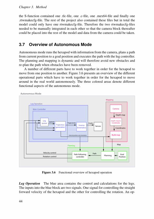
3.7 Overview of Autonomous Mode

Autonomous mode runs the hexapod with information from the camera, plans a pathfrom current position to a goal position and executes the path with the leg controller.The planning and mapping is dynamic and will therefore avoid new obstacles andre-plan the path when obstacles have been removed.

A number of different parts have to work together in order for the hexapod tomove from one position to another. Figure 3.6 presents an overview of the differentoperational parts which have to work together in order for the hexapod to movearound in the real world autonomously. The three colored areas denote differentfunctional aspects of the autonomous mode.

Leg Operation

Main Controller

Legqueue

queue

Trajectorygeneration

Inversekinematics

Servos

Camera

Trajectories Angles

Depth map

Depth map toCoordinates

Internal position and orientation

Coordinates

Build map

Planning

Map

Path-followingcontroller

PathVelocity control

Rotation control

Mapping

Planning

Autonomous Mode

Goal Position

Figure 3.6 Functional overview of hexapod operation

Leg Operation The blue area contains the control and calculations for the legs.The inputs into the blue block are two signals. One signal for controlling the straightforward velocity of the hexapod and the other for controlling the rotation. An op-

44

3.7 Overview of Autonomous Mode

tion could have been to include another control signal for controlling the sidewaysmovement. But the sideways signal was left out since it provided small practicaladvantages but would have added complexity to the path-following controller. Theleg queue block orders the legs with regards to which legs are the farthest behindthe others when it comes to following the velocity signal. The leg farthest behindwill be put first in the queue and the following legs in subsequent order. This queueis passed to the trajectory generation where discretized trajectories are created forall feet. These trajectories are based on the current position of all hexapod feet andtheir individual goal positions. The goal positions are calculated based on velocityand rotation control signals. The feet trajectories are fed to the inverse kinematicsblock. This block calculates the angles of all joints for the feet positions calculatedin the trajectory generation. These angles are then fed to the servos via the Arbotix-card. The actual movement is then performed by the internal PID-controllers in theDynamixel-servos [Thilderkvist and Svensson, 2015].

Mapping The red block contains all of the mapping calculations. It starts with aconnection to the ASUS depth camera. This provides a depth map which essentiallyis a matrix with depth values in every pixel. The depth map is sent to the coordi-nate transform block. This block uses information about the intrinsic parameters ofthe camera in addition to the depth map to create a point cloud. The point cloud isessentially a set of points in space which consists of x, y and z values. The pointcloud is cleaned by removing the floor which is assumed to be a plane. Reflectionsin windows can produce points which are unreasonably far away are removed. Theset of points are then sent to the map building block. This block combines the in-formation about obstacle coordinates in space and the robot position and rotationin a map. Obstacles are added and removed from the map depending on the points.A safety area is also added around all obstacles, in order for the hexapod to have amargin to avoid collisions.

Planning and Path-Following The green block performs all the planning opera-tions where the goal position is set by the user. The planning block then uses themap with start and goal position to plan a path from the current position to the goal.Planning is performed by building a road map from the discretized grid map. All ad-joining cells in the map are connected in the road map which is essentially a graph.An incremental heuristic search algorithm called D* lite is used to find a path in theroad map. The path shows which cells to traverse in order to reach the goal as fast aspossible. In order to follow the path, it is sent to the path-following controller. Eachway-point is transformed into continuous coordinates. The controller compares thecurrent position and rotation to the direction and distance of the next way-point inthe path. Errors in direction and distance from way-point are used to calculate con-trol signals. The controller used is essentially a proportional controller where theforward control signal is blocked if the rotational error is too large. Forward veloc-ity and rotation control signals are sent into the leg block and the feedback loop isclosed.

45

Chapter 3. Method

3.8 Real-Time Multi-threading

Simulink includes functionality for running multiple threads on one core. This iscalled multitasking operation in Simulink. All blocks running at the same samplingfrequency will be running as the same task. By default the priorities of the threadsare set so the fastest sampled thread will have the highest priority. The code gen-eration takes care of setting up threads and includes a scheduler [Simulink CoderUser’s guide].

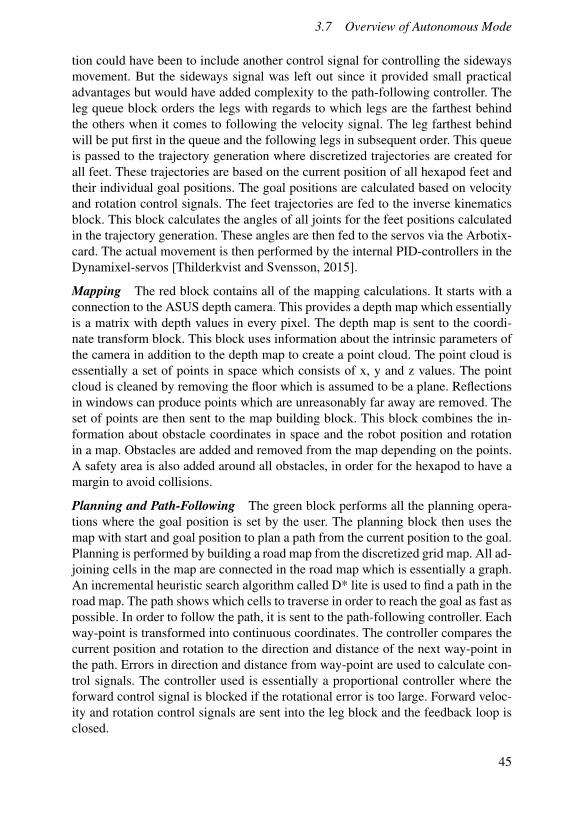
Different parts of the code are of varying importance and different sample fre-quencies are needed for robust operation. In Table 3.2 the sampling frequencies fordifferent parts of the code are presented. The leg operations have to be performed ata high sampling frequency for smooth operation of the legs. The leg operations areset to highest priority since they are more important than the other blocks. Morethorough testing of the sample frequency of the leg operations is performed in[Thilderkvist and Svensson, 2015]. Based on tests and [Thilderkvist and Svensson,2015] the leg operation can be seen to possess a bit less than half of the compu-tational power of the BeagleBone. The calculations of mapping and planning takeapproximately half a second to perform. The execution time of the path-following isnegligible compared to the leg, mapping and planning calculations. The sample rateof mapping and planning was set to one sample per second. With good multi-taskingbehavior the computational power should suffice to run the hexapod without inter-ruptions. The one-second sampling time for mapping and planning should sufficefor dynamic re-planning to work quickly enough.

Process Sampling frequency [Hz]

Leg operation 40

Mapping and Planning 1

Path-following 10

Table 3.2 Sampling frequencies

3.9 Positioning of the Hexapod

Inertial Measurement UnitTo calculate the positioning of the hexapod, different methods where analyzed.Since the robot already had an IMU integrated it would be convenient if the ac-celerometer in the IMU could be used to estimate the position of the hexapod inthe map. Unfortunately, the measurements were noisy and hard to read. A low-pass

46

3.9 Positioning of the Hexapod

filter was implemented as an attempt to make this better. Thereafter the filtered sig-nals were fed through double integrators in order to estimate the position out of theacceleration but large drift in the position was observed. This is to be expected whendouble integrators are applied since tiny errors in mounting of the IMU and noisemight yield large effects.

Internal velocity for positioningAs it would be time consuming to get the accelerometer to work properly. There-fore, it was decided to look for other methods. A simple heuristic way used forlocalization was to assume there is no uncertainty in the actuation of the controller.This way the trajectory for the feet will provide the position of the robot for eachtime step.

Point Cloud ProcessingThe planning is performed in 2 dimensions and all traversable surfaces are requiredto be flat. In order to build a map which represents all non-traversable areas asobstacles, the floor is to be found in the point cloud. With information about theorientation of the floor all points deviating more than a pre-determined thresholdcan be seen as obstacles. There are numerous ways of fitting a plane to a set ofpoints in space of which a simple method is using least squares regression. Thismethod will fit a plane to all points in space with a quadratic loss function. A resultof this will be that points farther from the fitting plane will influence the orientationmore than those close to it. The fitted plane will therefore be extremely biased andunpredictable unless the points are evenly distributed around the plane, for example,a Gaussian distribution. This case was highly unlikely, if not impossible, anothermethod taking into account a vast amount of outliers therefore has to be used.

Random Consensus Optimization (RANSOP)The RANSOP method was developed and tested in V-REP based on the assumptionthat the point clouds generated would be similar to those from the real camera. Itwas done by mounting the camera in a known position on the robot where the pos-sible movements of the robot are approximately known. This yields approximateinformation of the position and orientation of the floor plane related to the camera.This extra information was used to improve the RANSOP algorithm for these pur-poses. The goal was to reduce the computational power needed since the algorithmsare run in real-time. Another goal was to modify the algorithm so information aboutthe initial guess of the plane could be used for better results. The algorithm was onlyto find the floor plane and no others. Unfortunately, the floor from the real camerawas noisy and mostly incomplete. The use of RANSOP on the real robot thereforehad to be abandoned.

47

Chapter 3. Method

3.10 Mapping and Planning Overview

The mapping and planning methods are tightly connected since the planning algo-rithm will have to plan in the map. In other words, they will have to be compati-ble and chosen in tandem. A first realization is that saving all points of the pointcloud every sample will generate large amounts of data. However, it will not con-tribute with significant amount of extra information since many static objects willyield points in the same position. An interesting reasoning regarding the memoryneeds are discussed in the master’s thesis by Sara Gustafzelius [Gustafzelius, 2015],where data grow quickly if no simplification or reduction is performed. Therefore,a method for modeling the world in a more simple way is needed.

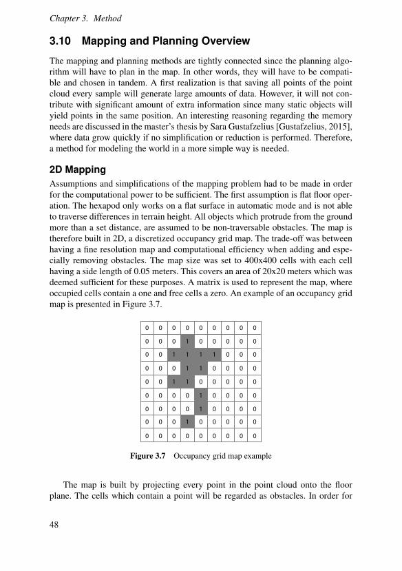
2D MappingAssumptions and simplifications of the mapping problem had to be made in orderfor the computational power to be sufficient. The first assumption is flat floor oper-ation. The hexapod only works on a flat surface in automatic mode and is not ableto traverse differences in terrain height. All objects which protrude from the groundmore than a set distance, are assumed to be non-traversable obstacles. The map istherefore built in 2D, a discretized occupancy grid map. The trade-off was betweenhaving a fine resolution map and computational efficiency when adding and espe-cially removing obstacles. The map size was set to 400x400 cells with each cellhaving a side length of 0.05 meters. This covers an area of 20x20 meters which wasdeemed sufficient for these purposes. A matrix is used to represent the map, whereoccupied cells contain a one and free cells a zero. An example of an occupancy gridmap is presented in Figure 3.7.

0 0 0 0 0 0 0 0 0

0 0 0 1 0 0 0 0 0

0 0 1 1 1 1 0 0 0

0 0 0 1 1 0 0 0 0

0 0 1 1 0 0 0 0 0

0 0 0 0 1 0 0 0 0

0 0 0 0 1 0 0 0 0

0 0 0 1 0 0 0 0 0

0 0 0 0 0 0 0 0 0

Figure 3.7 Occupancy grid map example

The map is built by projecting every point in the point cloud onto the floorplane. The cells which contain a point will be regarded as obstacles. In order for

48

3.10 Mapping and Planning Overview

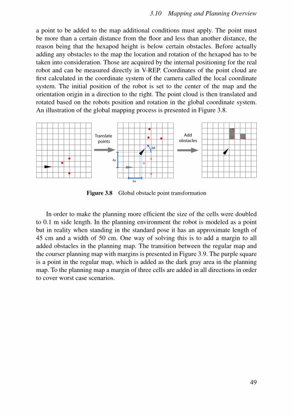
a point to be added to the map additional conditions must apply. The point mustbe more than a certain distance from the floor and less than another distance, thereason being that the hexapod height is below certain obstacles. Before actuallyadding any obstacles to the map the location and rotation of the hexapod has to betaken into consideration. Those are acquired by the internal positioning for the realrobot and can be measured directly in V-REP. Coordinates of the point cloud arefirst calculated in the coordinate system of the camera called the local coordinatesystem. The initial position of the robot is set to the center of the map and theorientation origin in a direction to the right. The point cloud is then translated androtated based on the robots position and rotation in the global coordinate system.An illustration of the global mapping process is presented in Figure 3.8.

Translate points

Addobstacles

Δx

Δθ

Δy

Figure 3.8 Global obstacle point transformation

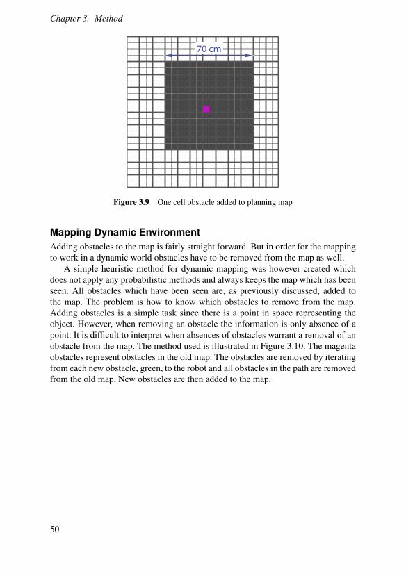
In order to make the planning more efficient the size of the cells were doubledto 0.1 m side length. In the planning environment the robot is modeled as a pointbut in reality when standing in the standard pose it has an approximate length of45 cm and a width of 50 cm. One way of solving this is to add a margin to alladded obstacles in the planning map. The transition between the regular map andthe courser planning map with margins is presented in Figure 3.9. The purple squareis a point in the regular map, which is added as the dark gray area in the planningmap. To the planning map a margin of three cells are added in all directions in orderto cover worst case scenarios.

49

Chapter 3. Method

70 cm

Figure 3.9 One cell obstacle added to planning map

Mapping Dynamic EnvironmentAdding obstacles to the map is fairly straight forward. But in order for the mappingto work in a dynamic world obstacles have to be removed from the map as well.

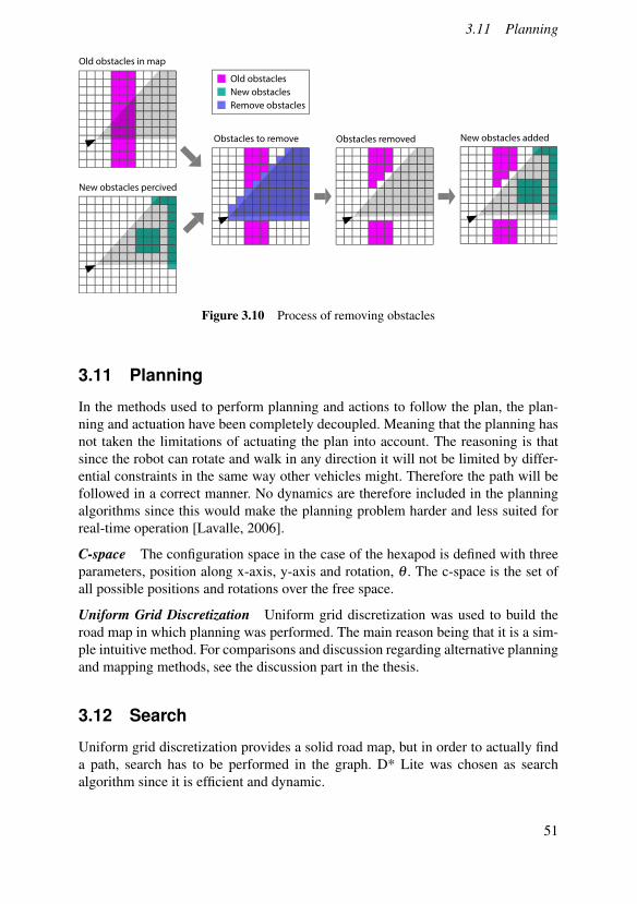
A simple heuristic method for dynamic mapping was however created whichdoes not apply any probabilistic methods and always keeps the map which has beenseen. All obstacles which have been seen are, as previously discussed, added tothe map. The problem is how to know which obstacles to remove from the map.Adding obstacles is a simple task since there is a point in space representing theobject. However, when removing an obstacle the information is only absence of apoint. It is difficult to interpret when absences of obstacles warrant a removal of anobstacle from the map. The method used is illustrated in Figure 3.10. The magentaobstacles represent obstacles in the old map. The obstacles are removed by iteratingfrom each new obstacle, green, to the robot and all obstacles in the path are removedfrom the old map. New obstacles are then added to the map.

50

3.11 Planning

Old obstacles in map

New obstacles percived

Old obstacles

New obstacles

Remove obstacles

Obstacles to remove Obstacles removed New obstacles added

Figure 3.10 Process of removing obstacles

3.11 Planning

In the methods used to perform planning and actions to follow the plan, the plan-ning and actuation have been completely decoupled. Meaning that the planning hasnot taken the limitations of actuating the plan into account. The reasoning is thatsince the robot can rotate and walk in any direction it will not be limited by differ-ential constraints in the same way other vehicles might. Therefore the path will befollowed in a correct manner. No dynamics are therefore included in the planningalgorithms since this would make the planning problem harder and less suited forreal-time operation [Lavalle, 2006].

C-space The configuration space in the case of the hexapod is defined with threeparameters, position along x-axis, y-axis and rotation, q . The c-space is the set ofall possible positions and rotations over the free space.

Uniform Grid Discretization Uniform grid discretization was used to build theroad map in which planning was performed. The main reason being that it is a sim-ple intuitive method. For comparisons and discussion regarding alternative planningand mapping methods, see the discussion part in the thesis.

3.12 Search

Uniform grid discretization provides a solid road map, but in order to actually finda path, search has to be performed in the graph. D* Lite was chosen as searchalgorithm since it is efficient and dynamic.

51

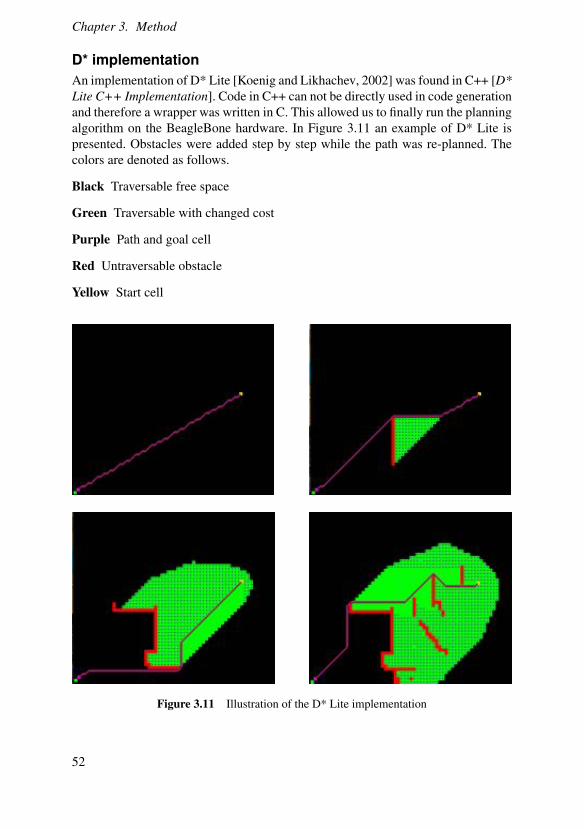
Chapter 3. Method

D* implementationAn implementation of D* Lite [Koenig and Likhachev, 2002] was found in C++ [D*Lite C++ Implementation]. Code in C++ can not be directly used in code generationand therefore a wrapper was written in C. This allowed us to finally run the planningalgorithm on the BeagleBone hardware. In Figure 3.11 an example of D* Lite ispresented. Obstacles were added step by step while the path was re-planned. Thecolors are denoted as follows.

Black Traversable free space

Green Traversable with changed cost

Purple Path and goal cell

Red Untraversable obstacle

Yellow Start cell

Figure 3.11 Illustration of the D* Lite implementation

52

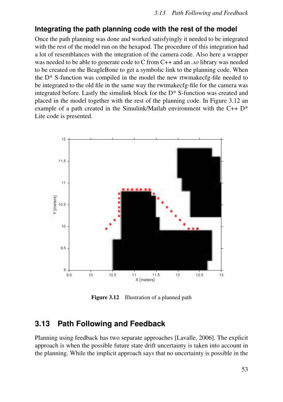
3.13 Path Following and Feedback

Integrating the path planning code with the rest of the modelOnce the path planning was done and worked satisfyingly it needed to be integratedwith the rest of the model run on the hexapod. The procedure of this integration hada lot of resemblances with the integration of the camera code. Also here a wrapperwas needed to be able to generate code to C from C++ and an .so library was neededto be created on the BeagleBone to get a symbolic link to the planning code. Whenthe D* S-function was compiled in the model the new rtwmakecfg-file needed tobe integrated to the old file in the same way the rwtmakecfg-file for the camera wasintegrated before. Lastly the simulink block for the D* S-function was created andplaced in the model together with the rest of the planning code. In Figure 3.12 anexample of a path created in the Simulink/Matlab environment with the C++ D*Lite code is presented.

X [meters]9.5 10 10.5 11 11.5 12 12.5 13

Y [

me

ters

]

9

9.5

10

10.5

11

11.5

12

Figure 3.12 Illustration of a planned path

3.13 Path Following and Feedback

Planning using feedback has two separate approaches [Lavalle, 2006]. The explicitapproach is when the possible future state drift uncertainty is taken into account inthe planning. While the implicit approach says that no uncertainty is possible in the

53

Chapter 3. Method

states. But a feedback plan is present which provides the actions to take in orderto revert back to the plan if it ends up in an unexpected state. Designing systemswith the explicit approach is more complicated, complexity is larger and algorithmsmore difficult to implement. We are using the implicit approach where planning isperformed by not taking into account the uncertainty in states, but instead correctsfor uncertainties with a control law.

Actuation for Path FollowingThere are three input signals which can be used for actuating the robot. These cor-respond to walking forward, walking sideways and rotating. The path which is tobe followed is a set of points, that is coordinates (x,y). An example of a path whichis to be followed is presented in Figure 3.12. The issue of following the path canbe seen as a control problem where the control signals have to be used in such away that the robot follows the path efficiently. The error in the control problem canbe seen as the distance between the robot and the next way-point in the path. Inorder to follow the path as smoothly as possible a couple of factors have to be takeninto account. First of all a decision has to be made by the robot regarding whichway-point to aim for. If a way-point to close is chosen the walking will be jerkyand change direction frequently and quickly. However, if a way-point goal is set toofar away the robot might cut corners and collide with obstacles. Another possibilityis to use numerous way-points at the same time so adjustments can be made fordirection of the next way-point even before the current one has been reached. Thiswould add a large amount of complexity and the controller was kept simple by justaiming for one way-point at the time. Since no differential constraints are imposedon the hexapod it can walk and rotate in the direction necessary for following thepath. A simple controller could therefore be used. It works by first checking if thecurrent way-point is closer than a set threshold. If so, choose the next point in thepath. If not, keep the current way-point as the goal. Then find the difference, eq , indirection between the current direction and the direction of the way-point. Use thedifference as the error in a proportional controller to minimize the direction error.If this direction error is below a magnitude threshold, walk forward. The error dis-tance, ed is used to decide when the way-point is close enough to start aiming forthe next way-point. In Figure 3.13 the errors used by the path-following controllerare used.

54

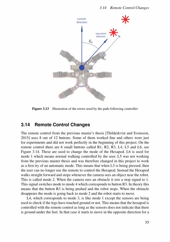
3.14 Remote Control Changes

current direction

way-pointdirection

ε

εd

Figure 3.13 Illustration of the errors used by the path-following controller

3.14 Remote Control Changes

The remote control from the previous master’s thesis [Thilderkvist and Svensson,2015] uses 8 out of 12 buttons. Some of them worked fine and others were justfor experiments and did not work perfectly in the beginning of this project. On theremote control there are 6 small buttons called R1, R2, R3, L4, L5 and L6, seeFigure 3.14. These are used to change the mode of the Hexapod. L6 is used formode 1 which means normal walking controlled by the user. L5 was not workingfrom the previous master thesis and was therefore changed in this project to workas a first try of an automatic mode. This means that when L5 is being pressed, thenthe user can no longer use the remote to control the Hexapod. Instead the Hexapodwalks straight forward and stops whenever the camera sees an object near the robot.This is called mode 2. When the camera sees an obstacle it sets a stop signal to 1.This signal switches mode to mode 4 which corresponds to button R3. In theory thismeans that the button R3 is being pushed and the robot stops. When the obstacledisappears the mode is going back to mode 2 and the robot starts to move.

L4, which corresponds to mode 3, is like mode 1 except the sensors are beingused to check if the legs have touched ground or not. This means that the hexapod iscontrolled with the remote control as long as the sensors does not indicate that thereis ground under the feet. In that case it starts to move in the opposite direction for a

55

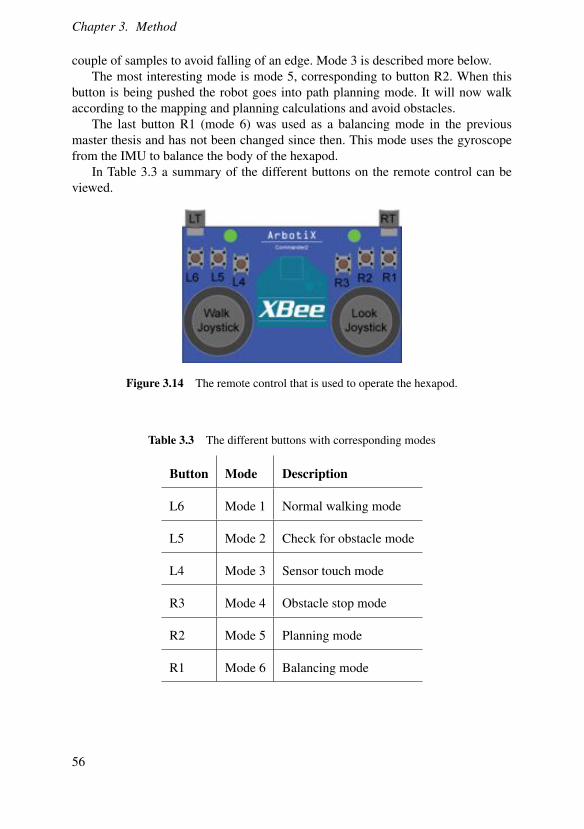
Chapter 3. Method

couple of samples to avoid falling of an edge. Mode 3 is described more below.The most interesting mode is mode 5, corresponding to button R2. When this

button is being pushed the robot goes into path planning mode. It will now walkaccording to the mapping and planning calculations and avoid obstacles.

The last button R1 (mode 6) was used as a balancing mode in the previousmaster thesis and has not been changed since then. This mode uses the gyroscopefrom the IMU to balance the body of the hexapod.

In Table 3.3 a summary of the different buttons on the remote control can beviewed.

Figure 3.14 The remote control that is used to operate the hexapod.

Table 3.3 The different buttons with corresponding modes

Button Mode Description

L6 Mode 1 Normal walking mode

L5 Mode 2 Check for obstacle mode

L4 Mode 3 Sensor touch mode

R3 Mode 4 Obstacle stop mode

R2 Mode 5 Planning mode

R1 Mode 6 Balancing mode

56

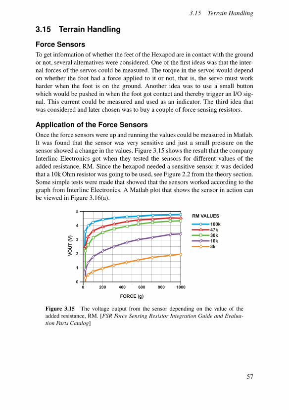
3.15 Terrain Handling

3.15 Terrain Handling

Force SensorsTo get information of whether the feet of the Hexapod are in contact with the groundor not, several alternatives were considered. One of the first ideas was that the inter-nal forces of the servos could be measured. The torque in the servos would dependon whether the foot had a force applied to it or not, that is, the servo must workharder when the foot is on the ground. Another idea was to use a small buttonwhich would be pushed in when the foot got contact and thereby trigger an I/O sig-nal. This current could be measured and used as an indicator. The third idea thatwas considered and later chosen was to buy a couple of force sensing resistors.

Application of the Force SensorsOnce the force sensors were up and running the values could be measured in Matlab.It was found that the sensor was very sensitive and just a small pressure on thesensor showed a change in the values. Figure 3.15 shows the result that the companyInterlinc Electronics got when they tested the sensors for different values of theadded resistance, RM. Since the hexapod needed a sensitive sensor it was decidedthat a 10k Ohm resistor was going to be used, see Figure 2.2 from the theory section.Some simple tests were made that showed that the sensors worked according to thegraph from Interlinc Electronics. A Matlab plot that shows the sensor in action canbe viewed in Figure 3.16(a).

Figure 3.15 The voltage output from the sensor depending on the value of theadded resistance, RM. [FSR Force Sensing Resistor Integration Guide and Evalua-tion Parts Catalog]

57

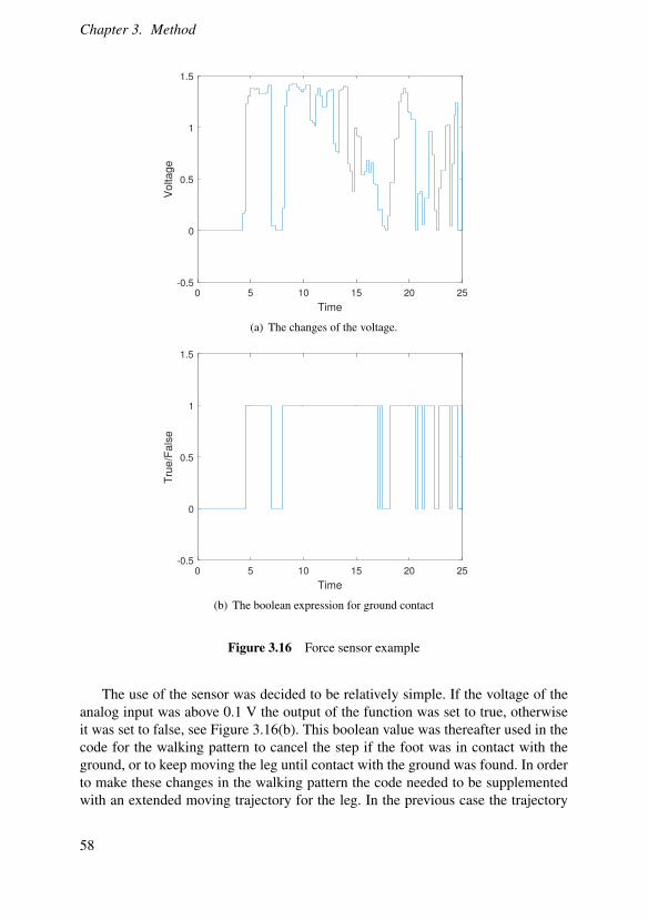
Chapter 3. Method

0 5 10 15 20 25

Time

-0.5

0

0.5

1

1.5

Volta

ge

(a) The changes of the voltage.

0 5 10 15 20 25

Time

-0.5

0

0.5

1

1.5

Tru

e/F

als

e

(b) The boolean expression for ground contact

Figure 3.16 Force sensor example

The use of the sensor was decided to be relatively simple. If the voltage of theanalog input was above 0.1 V the output of the function was set to true, otherwiseit was set to false, see Figure 3.16(b). This boolean value was thereafter used in thecode for the walking pattern to cancel the step if the foot was in contact with theground, or to keep moving the leg until contact with the ground was found. In orderto make these changes in the walking pattern the code needed to be supplementedwith an extended moving trajectory for the leg. In the previous case the trajectory

58

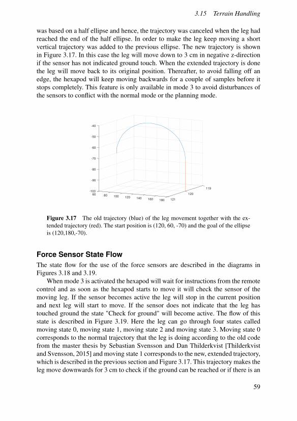
3.15 Terrain Handling

was based on a half ellipse and hence, the trajectory was canceled when the leg hadreached the end of the half ellipse. In order to make the leg keep moving a shortvertical trajectory was added to the previous ellipse. The new trajectory is shownin Figure 3.17. In this case the leg will move down to 3 cm in negative z-directionif the sensor has not indicated ground touch. When the extended trajectory is donethe leg will move back to its original position. Thereafter, to avoid falling off anedge, the hexapod will keep moving backwards for a couple of samples before itstops completely. This feature is only available in mode 3 to avoid disturbances ofthe sensors to conflict with the normal mode or the planning mode.

119

120

121

60 80 100 120 140 160 180

-100

-90

-80

-70

-60

-50

-40

Figure 3.17 The old trajectory (blue) of the leg movement together with the ex-tended trajectory (red). The start position is (120, 60, -70) and the goal of the ellipseis (120,180,-70).

Force Sensor State FlowThe state flow for the use of the force sensors are described in the diagrams inFigures 3.18 and 3.19.

When mode 3 is activated the hexapod will wait for instructions from the remotecontrol and as soon as the hexapod starts to move it will check the sensor of themoving leg. If the sensor becomes active the leg will stop in the current positionand next leg will start to move. If the sensor does not indicate that the leg hastouched ground the state "Check for ground" will become active. The flow of thisstate is described in Figure 3.19. Here the leg can go through four states calledmoving state 0, moving state 1, moving state 2 and moving state 3. Moving state 0corresponds to the normal trajectory that the leg is doing according to the old codefrom the master thesis by Sebastian Svensson and Dan Thilderkvist [Thilderkvistand Svensson, 2015] and moving state 1 corresponds to the new, extended trajectory,which is described in the previous section and Figure 3.17. This trajectory makes theleg move downwards for 3 cm to check if the ground can be reached or if there is an

59

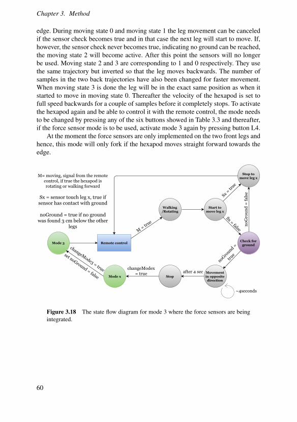
Chapter 3. Method

edge. During moving state 0 and moving state 1 the leg movement can be canceledif the sensor check becomes true and in that case the next leg will start to move. If,however, the sensor check never becomes true, indicating no ground can be reached,the moving state 2 will become active. After this point the sensors will no longerbe used. Moving state 2 and 3 are corresponding to 1 and 0 respectively. They usethe same trajectory but inverted so that the leg moves backwards. The number ofsamples in the two back trajectories have also been changed for faster movement.When moving state 3 is done the leg will be in the exact same position as when itstarted to move in moving state 0. Thereafter the velocity of the hexapod is set tofull speed backwards for a couple of samples before it completely stops. To activatethe hexapod again and be able to control it with the remote control, the mode needsto be changed by pressing any of the six buttons showed in Table 3.3 and thereafter,if the force sensor mode is to be used, activate mode 3 again by pressing button L4.

At the moment the force sensors are only implemented on the two front legs andhence, this mode will only fork if the hexapod moves straight forward towards theedge.

Figure 3.18 The state flow diagram for mode 3 where the force sensors are beingintegrated.

60

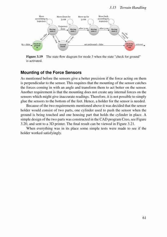
3.15 Terrain Handling

Figure 3.19 The state flow diagram for mode 3 when the state "check for ground"is activated.

Mounting of the Force SensorsAs mentioned before the sensors give a better precision if the force acting on themis perpendicular to the sensor. This requires that the mounting of the sensor catchesthe forces coming in with an angle and transform them to act better on the sensor.Another requirement is that the mounting does not create any internal forces on thesensors which might give inaccurate readings. Therefore, it is not possible to simplyglue the sensors to the bottom of the feet. Hence, a holder for the sensor is needed.

Because of the two requirements mentioned above it was decided that the sensorholder would consist of two parts, one cylinder used to push the sensor when theground is being touched and one housing part that holds the cylinder in place. Asimple design of the two parts was constructed in the CAD program Creo, see Figure3.20, and sent to a 3D printer. The final result can be viewed in Figure 3.21.

When everything was in its place some simple tests were made to see if theholder worked satisfyingly.

61

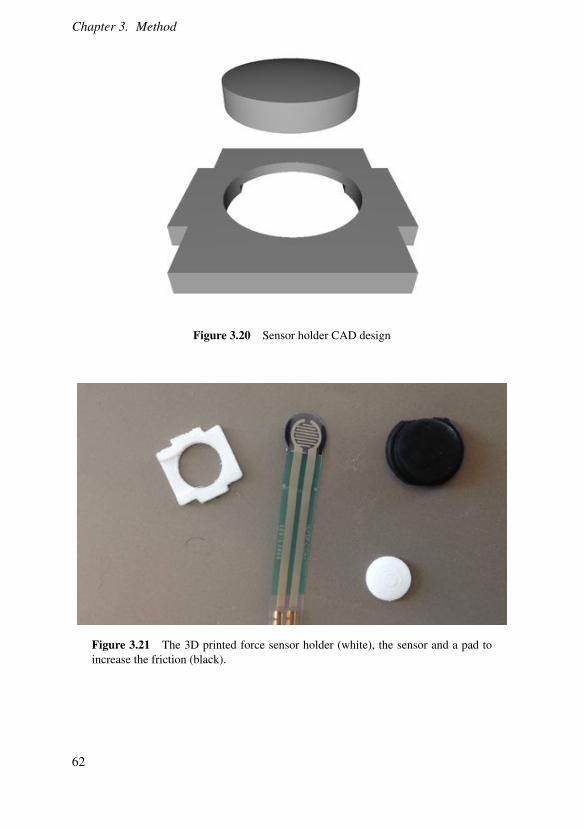
Chapter 3. Method

Figure 3.20 Sensor holder CAD design

Figure 3.21 The 3D printed force sensor holder (white), the sensor and a pad toincrease the friction (black).

62

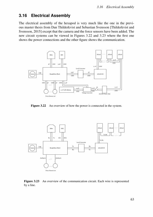
3.16 Electrical Assembly

3.16 Electrical Assembly

The electrical assembly of the hexapod is very much like the one in the previ-ous master thesis from Dan Thilderkvist and Sebastian Svensson [Thilderkvist andSvensson, 2015] except that the camera and the force sensors have been added. Thenew circuit systems can be viewed in Figures 3.22 and 3.23 where the first oneshows the power connections and the other figure shows the communication.

Figure 3.22 An overview of how the power is connected in the system.

Figure 3.23 An overview of the communication circuit. Each wire is representedby a line.

63

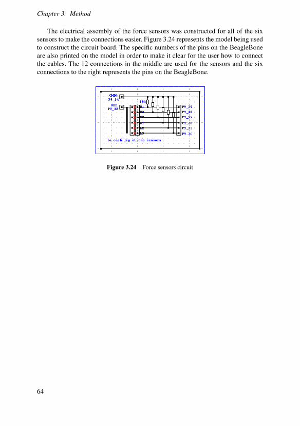
Chapter 3. Method

The electrical assembly of the force sensors was constructed for all of the sixsensors to make the connections easier. Figure 3.24 represents the model being usedto construct the circuit board. The specific numbers of the pins on the BeagleBoneare also printed on the model in order to make it clear for the user how to connectthe cables. The 12 connections in the middle are used for the sensors and the sixconnections to the right represents the pins on the BeagleBone.

Figure 3.24 Force sensors circuit

64

4

Results

In this chapter all the tests that have been made are described. This includes testsfor:

• RANSAC and RANSOP

• Mapping

• Complete planning test

• Force Sensors

For RANSAC and RANSOP tests were made both for the performance of the al-gorithms and comparisons of execution time. The tests for the Mapping were madein V-REP where the objective was to map an environment consisting of a couple ofobstacle.

The next tests were three trials to test the planning, mapping and path-following.Three different scenarios were tested, one without any obstacle, one with a staticobstacle and one test with a dynamic obstacle.

The last test performed was to see how well the force sensors and their imple-mentation worked. That included mounting of the sensors as well as the program-ming of the leg movements.

Before the different tests are described more thoroughly a quick review of thehexapod hardware changes are presented.

In Figure 4.1 the current hexapod can be seen. What is new since the beginningof this project is mainly the implementation of the camera and the force sensors.Some changes regarding the mounting of different parts have also been made.

65

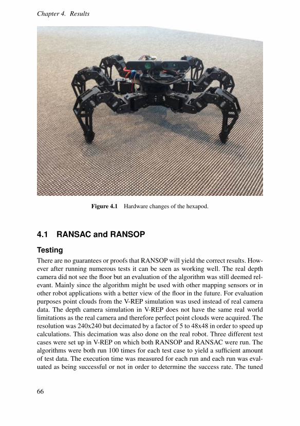
Chapter 4. Results

Figure 4.1 Hardware changes of the hexapod.

4.1 RANSAC and RANSOP

TestingThere are no guarantees or proofs that RANSOP will yield the correct results. How-ever after running numerous tests it can be seen as working well. The real depthcamera did not see the floor but an evaluation of the algorithm was still deemed rel-evant. Mainly since the algorithm might be used with other mapping sensors or inother robot applications with a better view of the floor in the future. For evaluationpurposes point clouds from the V-REP simulation was used instead of real cameradata. The depth camera simulation in V-REP does not have the same real worldlimitations as the real camera and therefore perfect point clouds were acquired. Theresolution was 240x240 but decimated by a factor of 5 to 48x48 in order to speed upcalculations. This decimation was also done on the real robot. Three different testcases were set up in V-REP on which both RANSOP and RANSAC were run. Thealgorithms were both run 100 times for each test case to yield a sufficient amountof test data. The execution time was measured for each run and each run was eval-uated as being successful or not in order to determine the success rate. The tuned

66

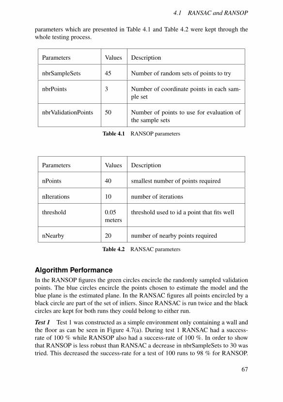
4.1 RANSAC and RANSOP

parameters which are presented in Table 4.1 and Table 4.2 were kept through thewhole testing process.

Parameters Values Description

nbrSampleSets 45 Number of random sets of points to try

nbrPoints 3 Number of coordinate points in each sam-ple set

nbrValidationPoints 50 Number of points to use for evaluation ofthe sample sets

Table 4.1 RANSOP parameters

Parameters Values Description

nPoints 40 smallest number of points required

nIterations 10 number of iterations

threshold 0.05meters

threshold used to id a point that fits well

nNearby 20 number of nearby points required

Table 4.2 RANSAC parameters

Algorithm PerformanceIn the RANSOP figures the green circles encircle the randomly sampled validationpoints. The blue circles encircle the points chosen to estimate the model and theblue plane is the estimated plane. In the RANSAC figures all points encircled by ablack circle are part of the set of inliers. Since RANSAC is run twice and the blackcircles are kept for both runs they could belong to either run.

Test 1 Test 1 was constructed as a simple environment only containing a wall andthe floor as can be seen in Figure 4.7(a). During test 1 RANSAC had a success-rate of 100 % while RANSOP also had a success-rate of 100 %. In order to showthat RANSOP is less robust than RANSAC a decrease in nbrSampleSets to 30 wastried. This decreased the success-rate for a test of 100 runs to 98 % for RANSOP.

67

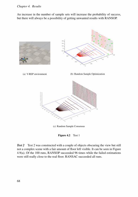
Chapter 4. Results

An increase in the number of sample sets will increase the probability of success,but there will always be a possibility of getting unwanted results with RANSOP.

(a) V-REP environment

2.5

2

1.5

1

0.5

0-1

-0.5

0

0.5

1

0

-0.2

0.4

0.6

0.2

(b) Random Sample Optimization

(c) Random Sample Consensus

Figure 4.2 Test 1

Test 2 Test 2 was constructed with a couple of objects obscuring the view but stillnot a complex scene with a fair amount of floor left visible. It can be seen in Figure4.9(a). Of the 100 runs, RANSOP succeeded 96 times while the failed estimationswere still really close to the real floor. RANSAC succeeded all runs.

68

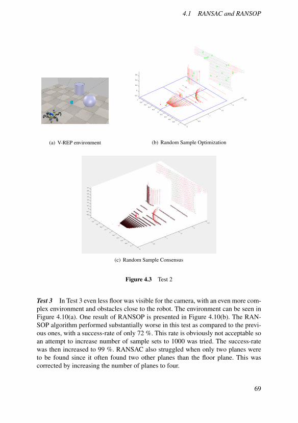
4.1 RANSAC and RANSOP

(a) V-REP environment

2.5

2

1.5

1

0.5

0

-1

-0.8

-0.6

-0.4

-0.2

0

0.2

0.4

0.6

0.8

1

0

-0.2

0.6

0.4

0.2

(b) Random Sample Optimization

(c) Random Sample Consensus

Figure 4.3 Test 2

Test 3 In Test 3 even less floor was visible for the camera, with an even more com-plex environment and obstacles close to the robot. The environment can be seen inFigure 4.10(a). One result of RANSOP is presented in Figure 4.10(b). The RAN-SOP algorithm performed substantially worse in this test as compared to the previ-ous ones, with a success-rate of only 72 %. This rate is obviously not acceptable soan attempt to increase number of sample sets to 1000 was tried. The success-ratewas then increased to 99 %. RANSAC also struggled when only two planes wereto be found since it often found two other planes than the floor plane. This wascorrected by increasing the number of planes to four.

69

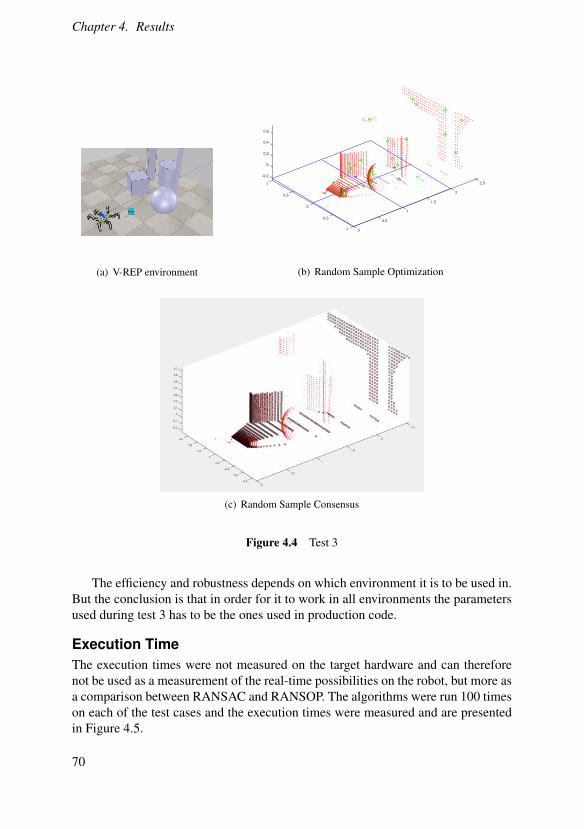
Chapter 4. Results

(a) V-REP environment

2.5

2

1.5

1

0.5

0-1

-0.5

0

0.5

0.4

-0.2

0

0.2

0.6

1

(b) Random Sample Optimization

(c) Random Sample Consensus

Figure 4.4 Test 3

The efficiency and robustness depends on which environment it is to be used in.But the conclusion is that in order for it to work in all environments the parametersused during test 3 has to be the ones used in production code.

Execution TimeThe execution times were not measured on the target hardware and can thereforenot be used as a measurement of the real-time possibilities on the robot, but more asa comparison between RANSAC and RANSOP. The algorithms were run 100 timeson each of the test cases and the execution times were measured and are presentedin Figure 4.5.

70

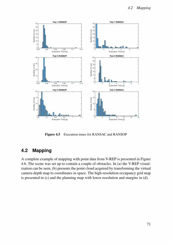
4.2 Mapping

Execution Time [s]0.02 0.04 0.06 0.08 0.1 0.12

Nu

mb

er

of

run

s

0

5

10

15

20

25

30

35Test 1 RANSOP

Execution Time [s]2 3 4 5 6 7

Nu

mb

er

of

run

s

0

5

10

15

20

25

30

35Test 1 RANSAC

Execution Time [s]0.02 0.04 0.06 0.08 0.1 0.12

Nu

mb

er

of

run

s

0

10

20

30

40Test 2 RANSOP

Execution Time [s]1 2 3 4 5 6 7

Nu

mb

er

of

run

s

0

5

10

15

20

25

30

35Test 2 RANSAC

Execution Time [s]0.6 0.7 0.8 0.9 1 1.1

Nu

mb

er

of

run

s

0

5

10

15

20Test 3 RANSOP

Execution Time [s]2 4 6 8 10 12 14

Nu

mb

er

of

run

s

0

5

10

15

20Test 3 RANSAC

Figure 4.5 Execution times for RANSAC and RANSOP

4.2 Mapping

A complete example of mapping with point data from V-REP is presented in Figure4.6. The scene was set up to contain a couple of obstacles. In (a) the V-REP visual-ization can be seen, (b) presents the point cloud acquired by transforming the virtualcamera depth map to coordinates in space. The high-resolution occupancy grid mapis presented in (c) and the planning map with lower resolution and margins in (d).

71

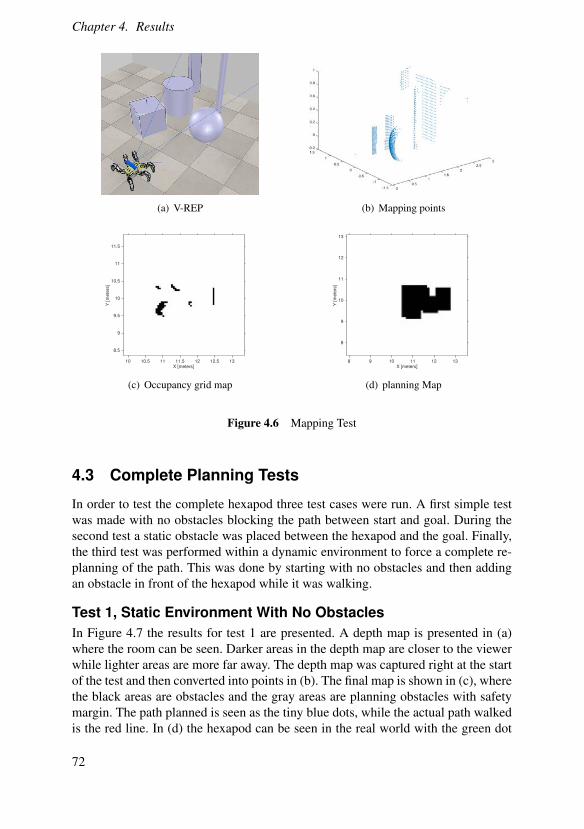
Chapter 4. Results

(a) V-REP (b) Mapping points

Binary Occupancy Grid

X [meters]10 10.5 11 11.5 12 12.5 13

Y [

me

ters

]

8.5

9

9.5

10

10.5

11

11.5

(c) Occupancy grid map

X [meters]8 9 10 11 12 13

Y [

me

ters

]

8

9

10

11

12

13

(d) planning Map

Figure 4.6 Mapping Test

4.3 Complete Planning Tests

In order to test the complete hexapod three test cases were run. A first simple testwas made with no obstacles blocking the path between start and goal. During thesecond test a static obstacle was placed between the hexapod and the goal. Finally,the third test was performed within a dynamic environment to force a complete re-planning of the path. This was done by starting with no obstacles and then addingan obstacle in front of the hexapod while it was walking.

Test 1, Static Environment With No ObstaclesIn Figure 4.7 the results for test 1 are presented. A depth map is presented in (a)where the room can be seen. Darker areas in the depth map are closer to the viewerwhile lighter areas are more far away. The depth map was captured right at the startof the test and then converted into points in (b). The final map is shown in (c), wherethe black areas are obstacles and the gray areas are planning obstacles with safetymargin. The path planned is seen as the tiny blue dots, while the actual path walkedis the red line. In (d) the hexapod can be seen in the real world with the green dot

72

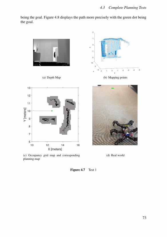
4.3 Complete Planning Tests

being the goal. Figure 4.8 displays the path more precisely with the green dot beingthe goal.

(a) Depth Map

-2

-1

0

10

1

2

z

x

5

y

0 -5-4-3-2-1012

(b) Mapping points

10 12 14 16

X [meters]

6

7

8

9

10

11

12

13

Y [m

ete

rs]

1010 1212 1414 1616

X [meters]X [meters]

66

77

88

99

1010

1111

1212

1313

Y [m

ete

rs]

Y [m

ete

rs]

(c) Occupancy grid map and correspondingplanning map

(d) Real world

Figure 4.7 Test 1

73

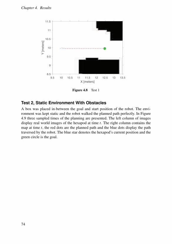
Chapter 4. Results

9.5 10 10.5 11 11.5 12 12.5 13 13.5

X [meters]

8.5

9

9.5

10

10.5

11

11.5

Y [m

ete

rs]

Figure 4.8 Test 1

Test 2, Static Environment With ObstaclesA box was placed in-between the goal and start position of the robot. The envi-ronment was kept static and the robot walked the planned path perfectly. In Figure4.9 three sampled times of the planning are presented. The left column of imagesdisplay real world images of the hexapod at time t. The right column contains themap at time t, the red dots are the planned path and the blue dots display the pathtraversed by the robot. The blue star denotes the hexapod’s current position and thegreen circle is the goal.

74

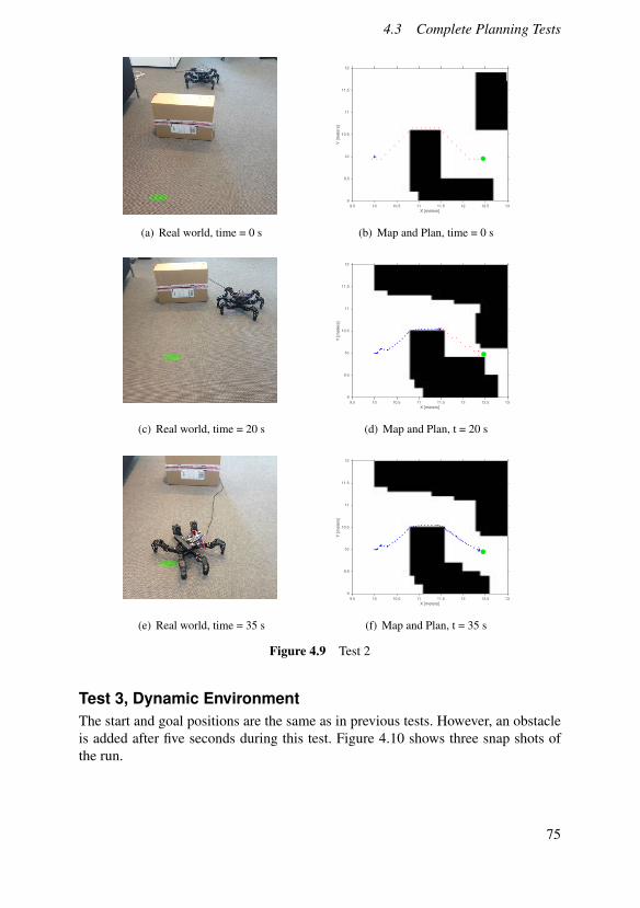
4.3 Complete Planning Tests

(a) Real world, time = 0 s

X [meters]9.5 10 10.5 11 11.5 12 12.5 13

Y [m

ete

rs]

9

9.5

10

10.5

11

11.5

12

(b) Map and Plan, time = 0 s

(c) Real world, time = 20 s

X [meters]9.5 10 10.5 11 11.5 12 12.5 13

Y [m

ete

rs]

9

9.5

10

10.5

11

11.5

12

(d) Map and Plan, t = 20 s

(e) Real world, time = 35 s

X [meters]9.5 10 10.5 11 11.5 12 12.5 13

Y [m

ete

rs]

9

9.5

10

10.5

11

11.5

12

(f) Map and Plan, t = 35 s

Figure 4.9 Test 2

Test 3, Dynamic EnvironmentThe start and goal positions are the same as in previous tests. However, an obstacleis added after five seconds during this test. Figure 4.10 shows three snap shots ofthe run.

75

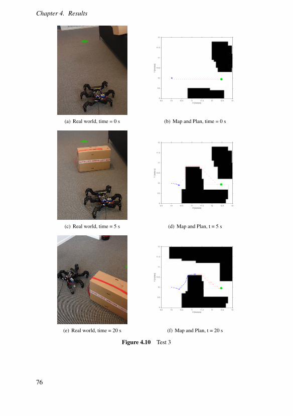
Chapter 4. Results

(a) Real world, time = 0 s

X [meters]9.5 10 10.5 11 11.5 12 12.5 13

Y [m

ete

rs]

9

9.5

10

10.5

11

11.5

12

(b) Map and Plan, time = 0 s

(c) Real world, time = 5 s

X [meters]9.5 10 10.5 11 11.5 12 12.5 13

Y [m

ete

rs]

9

9.5

10

10.5

11

11.5

12

(d) Map and Plan, t = 5 s

(e) Real world, time = 20 s

X [meters]9.5 10 10.5 11 11.5 12 12.5 13

Y [m

ete

rs]

9

9.5

10

10.5

11

11.5

12

(f) Map and Plan, t = 20 s

Figure 4.10 Test 3

76

4.4 Force Sensors

4.4 Force Sensors

To test the force sensors mode 3 was run on different terrains. The first test was tosee if the leg stopped earlier if the sensor got into contact with something aboveground, for example, a stone. This test was successful and the leg stopped at thecorrect position. The next test done was to see if the leg could keep going belowground level and then stop if the sensor indicated ground about one cm below theground level. Also this test was successful.

Finally, a test was made where the sensor never indicated ground. To do this testthe robot was placed on a table and was allowed to walk straight forward. Whenone of the front leg got to the edge it responded exactly as wanted and hence, thehexapod did not fall of the table.

The only time the tests were not successful was when the leg slipped in such away that the sensor never indicated ground touch.

At the moment the force sensors are only integrated on the two front legs, mainlybecause other things were prioritized before integrating them on every leg. Thismeans that the tests made above only works when the robot is moving towards theedge with its front.

77

5

Discussion and

Conclusions

5.1 Discussion

Simulink and Model-Based Design with Verification in V-REPSimulink has some advantages and disadvantages when it comes to building a map-ping and planning system. It has been convenient to generate code to the Beagle-Bone and small changes in the Simulink code can make for large differences inthe generated code which make for a fast testing and iteration process. However,when systems with large matrices or data structures have to be built it is better toimplement them in C/C++ or Matlab code and run it in the Simulink model.

SimMechanicsThere were a couple issues with modeling friction in SimMechanics. The contactfriction package in SimMechanics only supported friction between pre-set shapes,such as between a sphere and a plane. The robot is to interact with all sorts of shapesin the terrain. One solution might have been to approximate different shapes withlarge amounts of spheres or planes. This would mean that there had to be an ex-plicit friction model between all of these shapes and the feet. This is a cumbersomesolution when it comes to creating the SimMechanics model, which would needfriction blocks between all planes and the spheres on the feet. Another possible so-lution would be to change the position and orientation of the friction model planedepending on the topography of the terrain. So the same object would be used forall contacts between feet and ground, but this object would move to the positionof a foot when it was to be in contact with the ground. A similar solution was pro-posed by Burkus and Odry in a paper where they suggest modeling the ground usingpolygons generated by Matlab functions [Burkus and Odry, 2014].

78

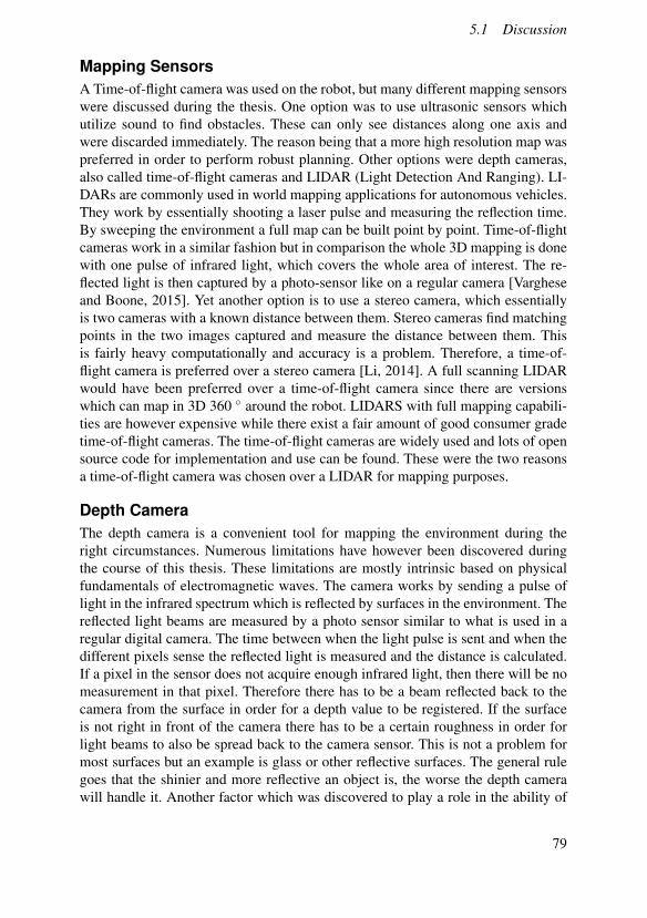
5.1 Discussion

Mapping SensorsA Time-of-flight camera was used on the robot, but many different mapping sensorswere discussed during the thesis. One option was to use ultrasonic sensors whichutilize sound to find obstacles. These can only see distances along one axis andwere discarded immediately. The reason being that a more high resolution map waspreferred in order to perform robust planning. Other options were depth cameras,also called time-of-flight cameras and LIDAR (Light Detection And Ranging). LI-DARs are commonly used in world mapping applications for autonomous vehicles.They work by essentially shooting a laser pulse and measuring the reflection time.By sweeping the environment a full map can be built point by point. Time-of-flightcameras work in a similar fashion but in comparison the whole 3D mapping is donewith one pulse of infrared light, which covers the whole area of interest. The re-flected light is then captured by a photo-sensor like on a regular camera [Vargheseand Boone, 2015]. Yet another option is to use a stereo camera, which essentiallyis two cameras with a known distance between them. Stereo cameras find matchingpoints in the two images captured and measure the distance between them. Thisis fairly heavy computationally and accuracy is a problem. Therefore, a time-of-flight camera is preferred over a stereo camera [Li, 2014]. A full scanning LIDARwould have been preferred over a time-of-flight camera since there are versionswhich can map in 3D 360 � around the robot. LIDARS with full mapping capabili-ties are however expensive while there exist a fair amount of good consumer gradetime-of-flight cameras. The time-of-flight cameras are widely used and lots of opensource code for implementation and use can be found. These were the two reasonsa time-of-flight camera was chosen over a LIDAR for mapping purposes.

Depth CameraThe depth camera is a convenient tool for mapping the environment during theright circumstances. Numerous limitations have however been discovered duringthe course of this thesis. These limitations are mostly intrinsic based on physicalfundamentals of electromagnetic waves. The camera works by sending a pulse oflight in the infrared spectrum which is reflected by surfaces in the environment. Thereflected light beams are measured by a photo sensor similar to what is used in aregular digital camera. The time between when the light pulse is sent and when thedifferent pixels sense the reflected light is measured and the distance is calculated.If a pixel in the sensor does not acquire enough infrared light, then there will be nomeasurement in that pixel. Therefore there has to be a beam reflected back to thecamera from the surface in order for a depth value to be registered. If the surfaceis not right in front of the camera there has to be a certain roughness in order forlight beams to also be spread back to the camera sensor. This is not a problem formost surfaces but an example is glass or other reflective surfaces. The general rulegoes that the shinier and more reflective an object is, the worse the depth camerawill handle it. Another factor which was discovered to play a role in the ability of

79

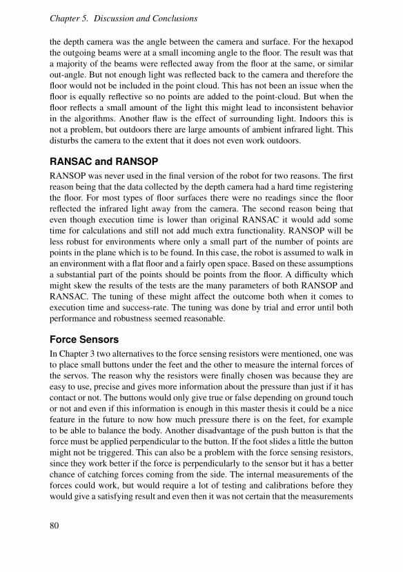
Chapter 5. Discussion and Conclusions

the depth camera was the angle between the camera and surface. For the hexapodthe outgoing beams were at a small incoming angle to the floor. The result was thata majority of the beams were reflected away from the floor at the same, or similarout-angle. But not enough light was reflected back to the camera and therefore thefloor would not be included in the point cloud. This has not been an issue when thefloor is equally reflective so no points are added to the point-cloud. But when thefloor reflects a small amount of the light this might lead to inconsistent behaviorin the algorithms. Another flaw is the effect of surrounding light. Indoors this isnot a problem, but outdoors there are large amounts of ambient infrared light. Thisdisturbs the camera to the extent that it does not even work outdoors.

RANSAC and RANSOPRANSOP was never used in the final version of the robot for two reasons. The firstreason being that the data collected by the depth camera had a hard time registeringthe floor. For most types of floor surfaces there were no readings since the floorreflected the infrared light away from the camera. The second reason being thateven though execution time is lower than original RANSAC it would add sometime for calculations and still not add much extra functionality. RANSOP will beless robust for environments where only a small part of the number of points arepoints in the plane which is to be found. In this case, the robot is assumed to walk inan environment with a flat floor and a fairly open space. Based on these assumptionsa substantial part of the points should be points from the floor. A difficulty whichmight skew the results of the tests are the many parameters of both RANSOP andRANSAC. The tuning of these might affect the outcome both when it comes toexecution time and success-rate. The tuning was done by trial and error until bothperformance and robustness seemed reasonable.

Force SensorsIn Chapter 3 two alternatives to the force sensing resistors were mentioned, one wasto place small buttons under the feet and the other to measure the internal forces ofthe servos. The reason why the resistors were finally chosen was because they areeasy to use, precise and gives more information about the pressure than just if it hascontact or not. The buttons would only give true or false depending on ground touchor not and even if this information is enough in this master thesis it could be a nicefeature in the future to now how much pressure there is on the feet, for exampleto be able to balance the body. Another disadvantage of the push button is that theforce must be applied perpendicular to the button. If the foot slides a little the buttonmight not be triggered. This can also be a problem with the force sensing resistors,since they work better if the force is perpendicularly to the sensor but it has a betterchance of catching forces coming from the side. The internal measurements of theforces could work, but would require a lot of testing and calibrations before theywould give a satisfying result and even then it was not certain that the measurements

80

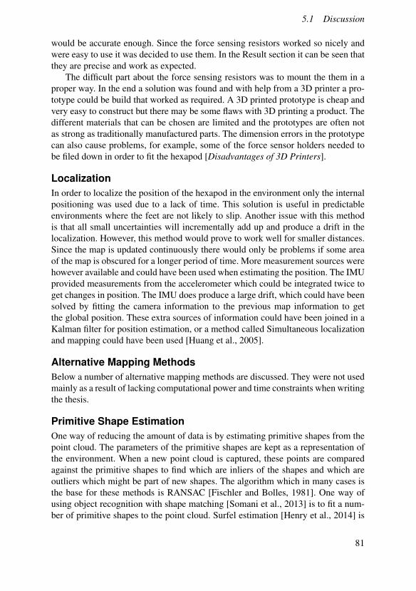
5.1 Discussion

would be accurate enough. Since the force sensing resistors worked so nicely andwere easy to use it was decided to use them. In the Result section it can be seen thatthey are precise and work as expected.

The difficult part about the force sensing resistors was to mount the them in aproper way. In the end a solution was found and with help from a 3D printer a pro-totype could be build that worked as required. A 3D printed prototype is cheap andvery easy to construct but there may be some flaws with 3D printing a product. Thedifferent materials that can be chosen are limited and the prototypes are often notas strong as traditionally manufactured parts. The dimension errors in the prototypecan also cause problems, for example, some of the force sensor holders needed tobe filed down in order to fit the hexapod [Disadvantages of 3D Printers].

LocalizationIn order to localize the position of the hexapod in the environment only the internalpositioning was used due to a lack of time. This solution is useful in predictableenvironments where the feet are not likely to slip. Another issue with this methodis that all small uncertainties will incrementally add up and produce a drift in thelocalization. However, this method would prove to work well for smaller distances.Since the map is updated continuously there would only be problems if some areaof the map is obscured for a longer period of time. More measurement sources werehowever available and could have been used when estimating the position. The IMUprovided measurements from the accelerometer which could be integrated twice toget changes in position. The IMU does produce a large drift, which could have beensolved by fitting the camera information to the previous map information to getthe global position. These extra sources of information could have been joined in aKalman filter for position estimation, or a method called Simultaneous localizationand mapping could have been used [Huang et al., 2005].

Alternative Mapping MethodsBelow a number of alternative mapping methods are discussed. They were not usedmainly as a result of lacking computational power and time constraints when writingthe thesis.

Primitive Shape EstimationOne way of reducing the amount of data is by estimating primitive shapes from thepoint cloud. The parameters of the primitive shapes are kept as a representation ofthe environment. When a new point cloud is captured, these points are comparedagainst the primitive shapes to find which are inliers of the shapes and which areoutliers which might be part of new shapes. The algorithm which in many cases isthe base for these methods is RANSAC [Fischler and Bolles, 1981]. One way ofusing object recognition with shape matching [Somani et al., 2013] is to fit a num-ber of primitive shapes to the point cloud. Surfel estimation [Henry et al., 2014] is

81

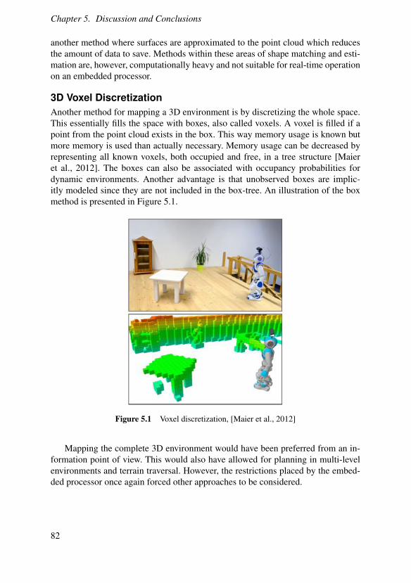
Chapter 5. Discussion and Conclusions

another method where surfaces are approximated to the point cloud which reducesthe amount of data to save. Methods within these areas of shape matching and esti-mation are, however, computationally heavy and not suitable for real-time operationon an embedded processor.

3D Voxel DiscretizationAnother method for mapping a 3D environment is by discretizing the whole space.This essentially fills the space with boxes, also called voxels. A voxel is filled if apoint from the point cloud exists in the box. This way memory usage is known butmore memory is used than actually necessary. Memory usage can be decreased byrepresenting all known voxels, both occupied and free, in a tree structure [Maieret al., 2012]. The boxes can also be associated with occupancy probabilities fordynamic environments. Another advantage is that unobserved boxes are implic-itly modeled since they are not included in the box-tree. An illustration of the boxmethod is presented in Figure 5.1.

Figure 5.1 Voxel discretization, [Maier et al., 2012]

Mapping the complete 3D environment would have been preferred from an in-formation point of view. This would also have allowed for planning in multi-levelenvironments and terrain traversal. However, the restrictions placed by the embed-ded processor once again forced other approaches to be considered.

82

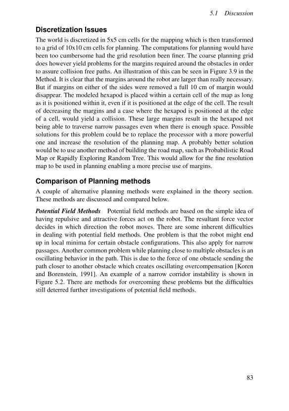
5.1 Discussion

Discretization IssuesThe world is discretized in 5x5 cm cells for the mapping which is then transformedto a grid of 10x10 cm cells for planning. The computations for planning would havebeen too cumbersome had the grid resolution been finer. The coarse planning griddoes however yield problems for the margins required around the obstacles in orderto assure collision free paths. An illustration of this can be seen in Figure 3.9 in theMethod. It is clear that the margins around the robot are larger than really necessary.But if margins on either of the sides were removed a full 10 cm of margin woulddisappear. The modeled hexapod is placed within a certain cell of the map as longas it is positioned within it, even if it is positioned at the edge of the cell. The resultof decreasing the margins and a case where the hexapod is positioned at the edgeof a cell, would yield a collision. These large margins result in the hexapod notbeing able to traverse narrow passages even when there is enough space. Possiblesolutions for this problem could be to replace the processor with a more powerfulone and increase the resolution of the planning map. A probably better solutionwould be to use another method of building the road map, such as Probabilistic RoadMap or Rapidly Exploring Random Tree. This would allow for the fine resolutionmap to be used in planning enabling a more precise use of margins.

Comparison of Planning methodsA couple of alternative planning methods were explained in the theory section.These methods are discussed and compared below.

Potential Field Methods Potential field methods are based on the simple idea ofhaving repulsive and attractive forces act on the robot. The resultant force vectordecides in which direction the robot moves. There are some inherent difficultiesin dealing with potential field methods. One problem is that the robot might endup in local minima for certain obstacle configurations. This also apply for narrowpassages. Another common problem while planning close to multiple obstacles is anoscillating behavior in the path. This is due to the force of one obstacle sending thepath closer to another obstacle which creates oscillating overcompensation [Korenand Borenstein, 1991]. An example of a narrow corridor instability is shown inFigure 5.2. There are methods for overcoming these problems but the difficultiesstill deterred further investigations of potential field methods.

83

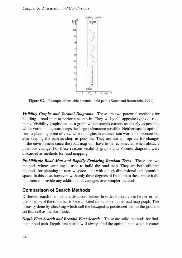
Chapter 5. Discussion and Conclusions

Figure 5.2 Example of unstable potential field path, [Koren and Borenstein, 1991]

Visibility Graphs and Voronoi Diagrams These are two potential methods forbuilding a road map to perform search in. They will yield opposite types of roadmaps. Visibility graphs creates a graph which rounds corners as closely as possiblewhile Voronoi diagrams keeps the largest clearance possible. Neither case is optimalfrom a planning point of view where margins in an uncertain world is important butalso keeping the path as short as possible. They are not appropriate for changesin the environment since the road map will have to be reconnected when obstaclepositions change. For these reasons visibility graphs and Voronoi diagrams werediscarded as methods for road mapping.

Probibilistic Road Map and Rapidly Exploring Random Trees These are twomethods where sampling is used to build the road map. They are both efficientmethods for planning in narrow spaces and with a high dimensional configurationspace. In this case, however, with only three degrees of freedom in the c-space it didnot seem to provide any additional advantages over simpler methods.

Comparison of Search MethodsDifferent search methods are discussed below. In order for search to be performedthe position of the robot has to be translated into a node in the road map graph. Thisis easily done by checking which cell the hexapod is positioned within the grid andset this cell as the start node.

Depth First Search and Breadth First Search These are solid methods for find-ing a good path. Depth-first search will always find the optimal path when it comes

84

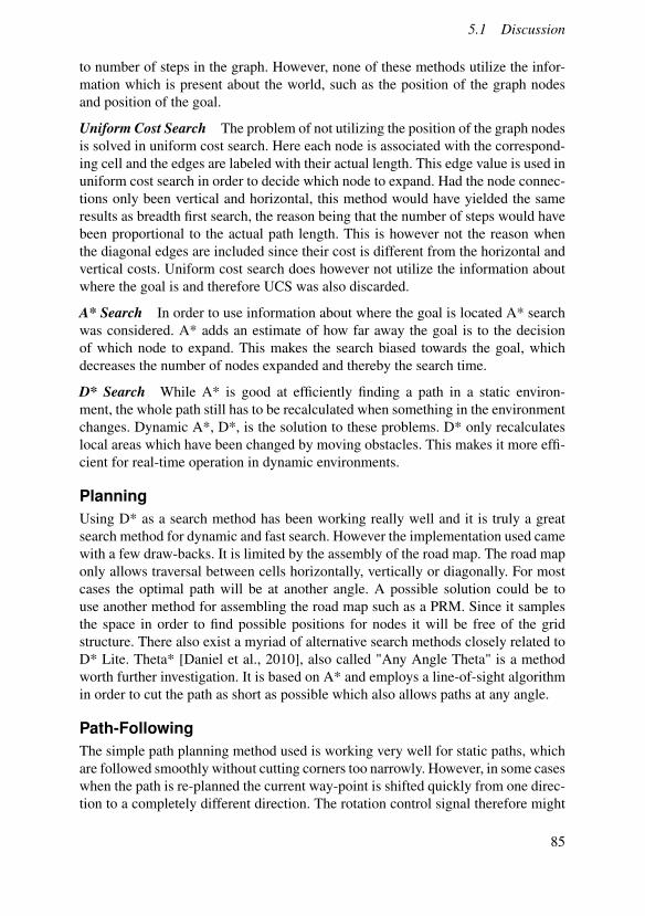
5.1 Discussion

to number of steps in the graph. However, none of these methods utilize the infor-mation which is present about the world, such as the position of the graph nodesand position of the goal.

Uniform Cost Search The problem of not utilizing the position of the graph nodesis solved in uniform cost search. Here each node is associated with the correspond-ing cell and the edges are labeled with their actual length. This edge value is used inuniform cost search in order to decide which node to expand. Had the node connec-tions only been vertical and horizontal, this method would have yielded the sameresults as breadth first search, the reason being that the number of steps would havebeen proportional to the actual path length. This is however not the reason whenthe diagonal edges are included since their cost is different from the horizontal andvertical costs. Uniform cost search does however not utilize the information aboutwhere the goal is and therefore UCS was also discarded.

A* Search In order to use information about where the goal is located A* searchwas considered. A* adds an estimate of how far away the goal is to the decisionof which node to expand. This makes the search biased towards the goal, whichdecreases the number of nodes expanded and thereby the search time.

D* Search While A* is good at efficiently finding a path in a static environ-ment, the whole path still has to be recalculated when something in the environmentchanges. Dynamic A*, D*, is the solution to these problems. D* only recalculateslocal areas which have been changed by moving obstacles. This makes it more effi-cient for real-time operation in dynamic environments.

PlanningUsing D* as a search method has been working really well and it is truly a greatsearch method for dynamic and fast search. However the implementation used camewith a few draw-backs. It is limited by the assembly of the road map. The road maponly allows traversal between cells horizontally, vertically or diagonally. For mostcases the optimal path will be at another angle. A possible solution could be touse another method for assembling the road map such as a PRM. Since it samplesthe space in order to find possible positions for nodes it will be free of the gridstructure. There also exist a myriad of alternative search methods closely related toD* Lite. Theta* [Daniel et al., 2010], also called "Any Angle Theta" is a methodworth further investigation. It is based on A* and employs a line-of-sight algorithmin order to cut the path as short as possible which also allows paths at any angle.

Path-FollowingThe simple path planning method used is working very well for static paths, whichare followed smoothly without cutting corners too narrowly. However, in some caseswhen the path is re-planned the current way-point is shifted quickly from one direc-tion to a completely different direction. The rotation control signal therefore might

85

Chapter 5. Discussion and Conclusions

go from the maximum positive value to the maximum negative value in one sample.This might result in jerky movements with the risk of leg collision. It can be some-what solved by lowering the allowed maximum rotational signal. In order to reallysolve the problem a low-pass filter might be used to filter out high frequencies andthereby blocking the quick changes.

Cornering IssuesOne issue found during testing was the issue of walking around obstacles whereonly the side of the obstacle facing the hexapod has been seen. When the hexapodrounds the corner it has never added the new side of the obstacle to the map. Sincethe TOF-camera has a blind distance the first 0.5 m it will never add and see theother side of the obstacle which increases the risk of collision, see Figure 5.3 foran example. Here can be seen how the green part of the obstacle is seen with thecamera, but the red parts are never added to the map. Since the hexapod wants toreach the goal right behind the obstacle the path is planned cutting the corner sincethat part of the obstacle never is added to the map.

Goal

Crash

Figure 5.3 Illustration of a failed corner rounding

One solution to this problem might be adding more hardware to the hexapod.Other sensors could pick up the slack within the dead zone of the camera. A coupleof ultrasound sensors could have been added just in order to avoid collision withclose obstacles, especially in a dynamic world.

Another possible solution could be to use a decision-making model for how thehexapod is supposed to traverse the path during different circumstances. It couldthen rotate and walk sideways around corners with a margin in order to map theother side of obstacles before trying to traverse those areas.

5.2 Conclusions

Overall this project has been successful, despite a lack of computational power andsome time consuming implementations, the hexapod became autonomous. V-REP

86

5.3 Future Improvements

has been a great way of testing algorithms before putting them on the hardware.It allowed for a much faster iteration testing process than testing directly on thehexapod would have been. Being able to plot all signals in real-time and havingcontrol of the environment also helped in the testing. Uncertainties in the real worldhave been a large issue during the thesis. Even though the planning and mappingalgorithms worked fine after testing in V-REP there were almost always issues whenmoving the testing onto the real hardware in the real world. With more testing andtweaking most of the algorithms ended up working fine.

The TOF camera has many positive aspects, despite issues in locating the floorand not being able to use it outdoors. It is a convenient and cheap solution for map-ping a complete 3D environment. Capturing the depth map was not at all computa-tionally heavy even though processing the point cloud was. Mapping the environ-ment in an accurate dynamic way has been a challenge. The errors in localizationof the position and rotation did not effect the map during the short tests which wererun. During longer tests it might have been problematic.

The planning part using D* Lite was tricky to implement using S-functions.However, it did work efficiently and with great results when it was implemented.

Finally, the terrain handling mode works really well. The force sensing resistorsused are sensitive, small and fairly cheap. The mounting generated some problemsbut in the end a solution was found that works satisfyingly. Since a 3D printer couldbe used the parts needed to mount the sensors were easy to construct.

The hexapod ended up being able to plan a path, avoid obstacles and handlesimple terrain. The potential improvements in performance, number of features androbustness in planning are immense.

5.3 Future Improvements

Many of the future improvements have been discussed as possibilities through-outthe thesis. One of the largest obstacles in development has been the computationalpower of the BeagleBone Black. It has a good processor which is sufficient for gen-erating trajectories, performing inverse kinematics and some mapping and planning.However for some of the methods, especially in a 3D environment, computationstend to become cumbersome.

Full 3D PlanningIn order to make the hexapod able to traverse terrain it would probably be necessaryto perform planning in a fully three dimensional model. Mapping a 3D environmentwas briefly mentioned earlier in the thesis, but was then discarded since it was toocomputationally heavy.

87

Chapter 5. Discussion and Conclusions

Mapping dynamic environments with probabilistic methodsThe mapping only contains two possible states, either a cell is occupied or it isfree. A more advanced system could be built where cells could be free, occupied oruncertain. The current version regards cells which have not been seen as free cells.Even though it actually is uncertain whether they are free or not. This informationcould be used to make more robust maps and planning. One example of how to usethe extra information is presented in [Hähnel et al., 2013].

Decision-MakingThe hexapod could be developed with a specific goal in mind. For example to mapthe environment or to search for a specific object. This would require some form ofdecision-theoretic model in order for the system to itself make decisions regardingwhere to walk.

Simultaneous Localization and MappingA better system for mapping and localizing the hexapod in the world would benecessary if the goal is to create accurate maps.

Force SensorsIn the future, one goal could be to apply the sensors to every foot and integrate themwith the balancing mode and thereby get the hexapod to re-balance as the legs arein different positions.

88

Bibliography

ASUS. Xtion pro live. http://www.asus.com/se/3D-Sensor/Xtion_PRO_LIVE/. Accessed: 2016-05-09.

BeagleBoard, F. Beaglebone black. https://beagleboard.org/black. Ac-cessed: 2016-06-03.

Burkus, E. and P. Odry (2014). Implementation of 3D Ground Contact Model forUneven Ground Using SimMechanics. Tech. rep. 10.1109/SISY.2014.6923572.Subotica Tech, Subotica, Serbia.

Cornell, S. Disadvantages of 3d printers. http://yourbusiness.azcentral.com/disadvantages-3d-printers-2212.html. Accessed: 2016-06-07.

Daniel, K., A. Nash, S. Koening, and A. Felner (2010). Theta*: Any-Angle PathPlanning on Grids. Tech. rep. Journal Of Artificial Intelligence Research, Vol-ume 39, pages 533-579, 2010, DOI: 10.1613/jair.2994. Computer Science De-partment University of Southern California, Los Angeles,USA. URL: http://www6.in.tum.de/Main/Publications/Somani2014a.pdf.

Eriksson, A. and M. Malmros (2016). Developer Manual, Artificial Intelligence andTerrain Handling of a Hexapod Robot. Users guide. Department of AutomaticControl, Lund University, Lund, Sweden.

Example of RANSAC. https://en.wikipedia.org/wiki/RANSAC. Figurereference, Accessed: 2016-06-09.

Fischler, M. A. and R. C. Bolles (1981). Random Sample Consensus: A Paradigmfor Model Fitting with Applications to Image Analysis and Automated Cartogra-phy. Tech. rep. ACM New York, NY, USA, Vol. 24, Issue 6, pp. 381-395, DOI:10.1145/358669.358692. Columbia University.

Gustafzelius, S. (2015). Dynamic path planning of initially unknown environmentsusing an RGB-D camera. Master’s Thesis TFRT--5980--SE. Department of Au-tomatic Control, Lund University, Lund, Sweden.

89

Bibliography

Henry, P., M. Krainin, E. Herbst, X. Ren, and D. Fox (2014). RGB-D Mapping: Us-ing Depth Cameras for Dense 3D Modeling of Indoor Environments. Researchpaper. Springer-Verlag GmbH Berlin Heidelberg, Vol. 79, DOI 10.1007/978-3-642-28572-1_33, Print ISBN: 978-3-642-28571-4, Online ISBN: 978-3-642-28572-1, Series ISSN: 1610-7438.

Huang, G., A. Rad, and Y. Wong (2005). Online SLAM in Dynamic Environments.Tech. rep. ICAR ’05. Proceedings., 12th International Conference on AdvancedRobotics, DOI: 10.1109/ICAR.2005.1507422, Print ISBN: 0-7803-9178-0. De-partment of Electrical Engineering, The Hong Kong Polytechnic University,Hong Kong.

Hähnel, D., R. Triebel, W. Burgard, and S. Thrun (2013). Map Building with MobileRobots in Dynamic Environments. Research Paper. Kluwer Academic Publish-ers, Vol. 19, Issue 1, DOI: 10.1007/s10514-005-0606-4, Print ISSN: 0929-5593,Online ISSN: 1573-7527. University of Freiburg, Department of Computer Sci-ence, Freiburg, Germany and Carnegie Mellon University, School of ComputerScience, PA, USA.

Interlink electronics. FSR Force Sensing Resistor Integration Guide and EvaluationParts Catalog. Users guide. Camarillo, CA, USA.

Koenig, S. and M. Likhachev (2002). D* Lite. Paper. American Association forArtificial Intelligence. Georgia Institute of Technology, Atlanta, USA, CarnegieMellon University, Pittsburgh, USA.

Koren, Y and J Borenstein (1991). Potential Field Methods and Their Inherent Lim-itations for Mobile Robot Navigation. Paper. Proceedings of the IEEE Confer-ence on Robotics and Automation, Sacramento, California, April 7-12, 1991,pp. 1398-1404. The University of Michigan.

Lavalle, S. M. (2006). Planning Algorithms. http://planning.cs.uiuc.edu.Cambridge University Press, Camebridge, UK.

Leonard, S. Potential field methods. http://www.cs.jhu.edu/~sleonard/week03.pdf. Accessed: 2016-03-17.

Li, L. (2014). Time-of-Flight Camera – An Introduction. Company Tech Report. Lit-erature number: SLOA190B, http://www.ti.com/lit/wp/sloa190b/sloa190b.pdf.Texas Instrument.

Maier, D., A. Hornung, and M. Bennewitz (2012). Real-Time Navigation in3D Environments Based on Depth Camera Data. Research Paper. 2012 12thIEEE-RAS International Conference on Humanoid Robots, DOI: 10.1109/HU-MANOIDS.2012.6651595, Print ISBN: 978-3-642-28571-4, ISSN: 2164-0572.University of Freiburg, Germany.

Mathworks. Matlab. http://se.mathworks.com/products/matlab/. Ac-cessed: 2016-06-02.

90

Bibliography

Mathworks. Simscape multibody contact forces library. http://www.mathworks.com / matlabcentral / fileexchange / 47417 - simscape - multibody -contact-forces-library. Accessed: 2016-02-02.

Mathworks. Simulink. http://se.mathworks.com/products/simulink/.Accessed: 2016-06-02.

Mathworks. Simulink Coder User’s guide. Users guide. URL: http : / / se .mathworks.com/help/pdf_doc/rtw/rtw_ug.pdf.

Mathworks. Understanding c code generation. http://se.mathworks.com/help/dsp/ug/understanding-code-generation.html. Accessed: 2016-05-31.

Microsoft. Kinect for windows sensor components and specifications. https://msdn.microsoft.com/en-us/library/jj131033.aspx. Accessed: 2016-05-09.

Neufeld, J. D* lite c++ implementation. https://github.com/ArekSredzki/dstar-lite. Accessed: 2016-03-11.

Picture of FSR. http : / / www . sedoniatech . co . nz / force - sensing -resistor-touch-sensor.htm. Figure reference, Accessed: 2016-05-25.

Robotics, C. Coppeliarobotics.com. http://www.coppeliarobotics.com. Ac-cessed: 2016-02-02.

Robotics, C. Designing dynamic simulations. http://www.coppeliarobotics.com / helpFiles / en / designingDynamicSimulations . htm. Accessed:2016-02-02.

Robotics, C. Enabling the Remote API - client side. http : / / www .coppeliarobotics.com/helpFiles/en/remoteApiClientSide.htm.Accessed: 2016-02-02.

Robotics, C. Remote API modus operandi. http://www.coppeliarobotics.com/helpFiles/en/remoteApiModusOperandi.htm. Accessed: 2016-02-02.

Russel, S. and P. Norvig (2010). Artificial Intelligence, A Modern Approach. http://aima.cs.berkeley.edu. Pearson Education, New Jersey, USA.

Somani, N., C. Cai, A. Perzylo, M. Rickert, and A. Knoll (2013). ObjectRecognition using constraints from Primitive Shape Matching. Paper. DOI:10.1007/978-3-319-14249-4_75, Print ISBN: 978-3-319-14248-7, OnlineISBN: 978-3-319-14249-4, ISSN: 0302-9743. Cyber-Physical Systems, fortiss- An-Institut der Technischen Universität München. Technische UniversitätMünchen, Fakultät für Informatik.

Structure. Openni 2 sdk binaries & docs. http://structure.io/openni. Ac-cessed: 2016-02-02.

91

Bibliography

Thilderkvist, D. and S. Svensson (2015). Motion Control of Hexapod Robot UsingModel-Based Design. Master’s Thesis TFRT--5971--SE. Department of Auto-matic Control, Lund University, Lund, Sweden.

Varghese, J. and R. Boone (2015). Overview of Autonomous Vehicle Sensors andSystems. Tech. rep. Proceedings of the 2015 International Conference on Oper-ations Excellence and Service Engineering Orlando, Florida, USA, September10-11, 2015, pp. 178-191. Department of Electrical Engineering, University ofMichigan, United States.

92

Document name

Date of issue

Document Number

Author(s) Supervisor

Sponsoring organization

Title and subtitle

Abstract

Keywords

Classification system and/or index terms (if any)

Supplementary bibliographical information

ISSN and key title ISBN

Language Number of pages Recipient’s notes

Security classification