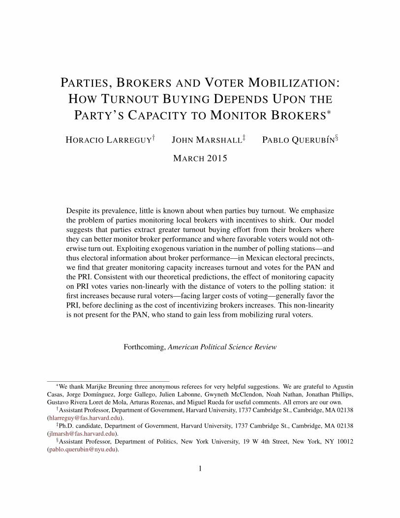
PARTIES, BROKERS AND VOTER MOBILIZATION:HOW TURNOUT BUYING DEPENDS UPON THE

PARTY’S CAPACITY TO MONITOR BROKERS∗

HORACIO LARREGUY† JOHN MARSHALL‡ PABLO QUERUBIN§

MARCH 2015

Despite its prevalence, little is known about when parties buy turnout. We emphasizethe problem of parties monitoring local brokers with incentives to shirk. Our modelsuggests that parties extract greater turnout buying effort from their brokers wherethey can better monitor broker performance and where favorable voters would not oth-erwise turn out. Exploiting exogenous variation in the number of polling stations—andthus electoral information about broker performance—in Mexican electoral precincts,we find that greater monitoring capacity increases turnout and votes for the PAN andthe PRI. Consistent with our theoretical predictions, the effect of monitoring capacityon PRI votes varies non-linearly with the distance of voters to the polling station: itfirst increases because rural voters—facing larger costs of voting—generally favor thePRI, before declining as the cost of incentivizing brokers increases. This non-linearityis not present for the PAN, who stand to gain less from mobilizing rural voters.

Forthcoming, American Political Science Review

∗We thank Marijke Breuning three anonymous referees for very helpful suggestions. We are grateful to AgustinCasas, Jorge Domınguez, Jorge Gallego, Julien Labonne, Gwyneth McClendon, Noah Nathan, Jonathan Phillips,Gustavo Rivera Loret de Mola, Arturas Rozenas, and Miguel Rueda for useful comments. All errors are our own.†Assistant Professor, Department of Government, Harvard University, 1737 Cambridge St., Cambridge, MA 02138

(hlarreguy@fas.harvard.edu).‡Ph.D. candidate, Department of Government, Harvard University, 1737 Cambridge St., Cambridge, MA 02138

(jlmarsh@fas.harvard.edu).§Assistant Professor, Department of Politics, New York University, 19 W 4th Street, New York, NY 10012

(pablo.querubin@nyu.edu).

1

Voter mobilization is an essential component of the electoral strategy of parties in every part

of the world. When the ballot is secret, parties seek to ensure that voters that are likely to support

the party turn out to vote (e.g. Cox and Kousser 1981; Nichter 2008). Common mobilization

strategies—including door-to-door or telephone campaigns, transporting voters to the polling sta-

tion, and turnout buying—rely on the superior knowledge of local mobilizers about the political

preferences of individual voters, which enables them to identify supporters that would not have

otherwise turned out. Mobilizers may not require payment when their interests are aligned with

their party’s.1 However, parties must often hire brokers without aligned incentives.

In this article, we focus on voter mobilization through hired brokers. While the exchange of

goods for voters turning out is widely reported in developing contexts (e.g. Nichter 2008; Nichter

and Palmer-Rubin 2014), such turnout buying is not uncommon in the developed world.2 Despite

the apparent extent of this phenomenon—which has the potential to substantially alter electoral

outcomes (Keefer 2007), and is illegal in many countries—little is understood about the conditions

that explain its prevalence.

As far as turnout buying can be gauged, it varies substantially across localities and political

parties. Theoretical work has only recently begun to explore when parties pursue different electoral

strategies (Gans-Morse, Mazzuca and Nichter 2013), and has yet to incorporate the principal-agent

relationship between parties and brokers. In this article, we extend existing theory and exploit a

natural experiment in Mexico to address a major question in the voter mobilization literature: when

1For example, labor unions (Gray and Caul 2000; Larreguy, Montiel and Querubın 2014; Leighley andNagler 2007), politically-motivated business and neighborhood associations (Cox, Rosenbluth and Thies1998; Holland and Palmer-Rubin 2014), and partisan volunteer canvassers (Nickerson, Friedrichs and King2006) often mobilize voters. Similarly, the career incentives of mobilizers may induce alignment with theparty (e.g. Szwarcberg 2012b).

2In 2004, Democratic party operatives were convicted for turnout buying (Nichter 2008), while thispractice has been part of elections in Texas for decades (“Texas Vote-Buying Case Casts Glare on Traditionof Election Day Goads,” The New York Times, January 12th 2014). Vote buying was also widely documentedin U.S. cities around the turn of the twentieth century (e.g. Cox and Kousser 1981; Rakove 1976; Wilson1960), and has more recently been observed in southern Europe (e.g. Chubb 1982; Kitschelt and Wilkinson2007).

2

do political parties hire brokers to mobilize potential voters?

While previous research has primarily focused on the monitoring problem between parties and

voters under a secret ballot (e.g. Cox and Kousser 1981; Nichter 2008; Stokes 2005), limited at-

tention has been paid to the relationship between parties and political brokers. This relative neglect

is surprising given that brokers typically implement voter mobilization strategies on election day

because they are better informed about the preferences of individual voters than political parties

(e.g. Finan and Schechter 2012; Stokes et al. 2013). Stokes et al. (2013) treat this interaction

between parties and brokers principally as a selection problem for political parties seeking to em-

ploy the best-connected brokers. However, because brokers are often hired contractors rather than

actors with incentives closely tied to political parties, this misses a critical moral hazard concern:

political parties hire brokers to mobilize likely supporters that would not otherwise turn out, but

brokers face strong incentives to shirk given that parties cannot easily monitor their actions.

Guided by this party-broker monitoring problem and our qualitative understanding of party-

broker relations in Mexico, we formalize a simple model predicting the conditions under which

parties hire brokers to mobilize voters. In our model, voters vary in their cost of voting—determined

by the distance to their polling station—and their ideological affinity, which determines their pref-

erence over parties. To capture differential knowledge of voter types, we assume parties do not

observe the preferences of individual voters, whereas local brokers know which party each voter

would vote for if they turned out. Parties thus hire political brokers to mobilize their pool of “po-

tential voters”—favorable voters that face prohibitive costs of turning out. Brokers can exert costly

effort to provide voters with incentives to turn out. However, the probability that a party is able to

infer broker effort after the election varies across electoral precincts. Given brokers will shirk if

they believe that they can go undetected and still receive payment, parties can buy more turnout in

locations where their monitoring capacity is greater.

Furthermore, the magnitude of the positive effect of monitoring capacity on turnout buying dif-

fers across political parties and depends on the distance of voters to the polling station. First, parties

3

that are relatively popular among rural voters—who face higher costs of traveling to vote—have

most to gain from the greater broker effort that increased monitoring capacity permits. Conversely,

there are fewer potential voters for predominantly urban parties to mobilize. Second, where the

cost to brokers of mobilizing voters increases sharply with distance, hiring brokers becomes pro-

hibitively costly—even for predominantly rural parties—once voters live sufficiently far from the

polling station. Among parties that do well in rural areas, our model thus predicts an “inverted-

U” relationship between the average distance of voters to the polling station and turnout buying.

Among urban parties, the increasing cost of hiring brokers quickly overpowers the declining pool

of potential voters as the distance to the polling station increases.

We take these theoretical insights to the data in Mexico. Despite emerging from seven decades

of one-party rule by the Institutional Revolutionary Party (PRI) in the 1990s, Mexican elections are

still characterized by clientelism and electoral mobilization. We focus on turnout buying—which

occurs outside deeply embedded clientelistic structures (see e.g. Cornelius 2004; Diaz-Cayeros,

Estevez and Magaloni forthcoming; Fox 1994; Magaloni 2006)—just before and especially on

election day. Mexico’s main political parties continue to engage in extensive turnout buying, offer-

ing gifts in exchange for turning out and illegally hiring buses and taxis to drive voters to polling

stations.3 Brokers hired by political parties play the essential intermediary role in this process,

mobilizing voters on election day in exchange for cash and bonuses (or sanctions) based on local

electoral performance (Ugalde and Rivera Loret de Mola 2013).

To test the model’s predictions for party vote shares, we leverage two sources of variation. First,

differences in monitoring capacity arise from an electoral rule requiring that a new polling station

is created for every 750 registered voters in an electoral precinct. Qualitative evidence indicates

that political parties use polling station-level electoral outcomes to reward their brokers. Each

additional polling station allows the party to better distinguish the effort of their broker from voter-

3See summaries such as Nichter and Palmer-Rubin (2014) and Ugalde and Rivera Loret de Mola (2013),and many reports including Alianza Cıvica, Boletın de Prensa, July 3rd 2012 and those in footnote 8.

4

level shocks affecting turnout. Information from more electoral returns thus increase the signal

to noise ratio surrounding the effect of broker effort on electoral outcomes, allowing the party to

better detect when their broker has shirked. Since new polling stations are constructed adjacent to

existing polling stations, the cost of traveling to the polling station remains constant. Second, we

exploit variation in political preferences and the cost of voting by calculating the average distance

that voters must travel to their precinct’s polling booth. Like many other developing countries,

including India, South Africa and Thailand, Mexico’s urban-rural political divide means that more

rural precincts where the average voter lives further from the polling station are less likely to turn

out and more likely to support a particular party—the PRI, in the case of Mexico.

We use a regression discontinuity design to compare polling stations in essentially identical

electoral precincts just above and just below the threshold for creating a new polling station. Our

results provide evidence of turnout buying consistent with our theoretical model: each additional

polling station increases electoral turnout by around one percentage point, significantly increasing

the vote share of the right-wing National Action Party (PAN) and especially the PRI. The vote share

of the Party of the Democratic Revolution (PRD), which has recently campaigned against vote-

buying practices and likely inherited the weakest political machines from the PRI, is unaffected.

Following our theoretical model, we also examine how the effect of an additional polling station

varies with distance. Consistent with our theory, the increase in the PRI vote at the discontinuity is

non-linear with distance. At the effect’s peak—where, on average, voters live around 1.5km from

the polling station—the PRI gains the vote of more than one percent of registered voters. This

interaction is if anything instead negative for the PAN, who stand to gain less from mobilizing

rural voters. These heterogeneous effects also dismiss alternative explanations. First, reduced

waiting time at the polling booth cannot explain why there is no increase in PRD votes or why the

effect on the PRI votes is non-linear with distance from the polling station. Second, if parties were

buying votes rather than turnout, we would expect to instead observe that an additional polling

station would differentially benefit the PRI in urban areas and benefit the PAN and PRD in rural

5

areas.

Although our estimates only account for around a 2.5 percent increase in votes for the PRI and

PAN, our empirical strategy only focuses on a single dimension of monitoring that can be cleanly

identified. Furthermore, given the differences in monitoring capacity are relatively small, our

estimates are quite substantial. Ultimately, our results demonstrate the importance of monitoring

in explaining differences in turnout buying across parties and geographic locations, but only point

at the tip of the iceberg of turnout-buying practices.

Our theoretical argument contributes to a nascent literature focusing on the intermediary role

of political brokers.4 This literature departs from extant work assuming that parties do not require

brokers or that broker interests are always aligned with their parties. Whereas Stokes et al. (2013)

treat hiring brokers as an adverse selection problem and Camp (2012) focuses on the collective ac-

tion problem for brokers, our model emphasizes the moral hazard problem arising from the party’s

inability to always monitor broker effort. While Larreguy (2013) focuses on the signal extraction

problem for brokers mediating clientelistic relationships, our model shows how heterogeneity in

voter preferences and the costs of voting causes parties to face differential incentives when mo-

bilizing voters outside clientelistic structures. Third, our model extends Gans-Morse, Mazzuca

and Nichter (2013) by introducing an agency problem that de-links party strategies from voting

outcomes. While their model suggests that the party-voter monitoring problem increases turnout

buying, we show that the party-broker monitoring problem instead decreases turnout buying.

Empirically, our results extend the existing literature in several ways. First, unlike previous

studies examining the effects of institutions on vote buying (Cox and Kousser 1981; Leon 2013),

we instead explain variation in turnout buying and exploit a powerful research design to iden-

tify causal effects consistent with our monitoring explanation. Second, we identify the conditions

4There is also a growing formal literature examining the monitoring mechanisms employed by bro-kers, rather than parties, vis-a-vis voters (e.g. Gingerich and Medina 2013; Rueda forthcoming; Smith andBueno de Mesquita 2012); Robinson and Verdier (2013) also consider the reverse credibility problem. Ourstudy, however, focuses on party monitoring of brokers.

6

under which parties interact effectively with brokers in a way that exclusively qualitative and ob-

servational accounts cannot (e.g. Levitsky 2014; Stokes et al. 2013; Szwarcberg 2012a; Wang and

Kurzman 2007). Finally, our study provides further evidence for the occurrence of turnout buy-

ing (see e.g. Nichter and Palmer-Rubin 2014), and suggests—like recent studies of vote buying

(Cantu 2014a; Finan and Schechter 2012; Gingerich 2014; Gonzalez-Ocantos et al. 2012; Vicente

2014)—that it can be effective at gaining votes. Fourth, our findings reinforce claims from con-

texts as diverse as Chicago, Colombia and India that political parties use disaggregated electoral

information to monitor the performance of their brokers (e.g. Rakove 1976, Rueda 2013).5

The article is structured as follows. We first provide a qualitative overview of elections and the

role of brokers in Mexico. The following section presents our theoretical model. We then describe

our data and explain our identification strategy, before presenting our results. We conclude with a

discussion of our findings.

Qualitative evidence of electoral manipulation in Mexico

Mexico has experienced a long history of electoral malpractice. During its 71-year stranglehold on

power extending back to 1929, the PRI was widely acknowledged to have engaged in clientelistic

transfers, vote buying and electoral fraud (e.g. Cornelius 2004; Magaloni 2006). After allega-

tions of widespread vote-rigging in the 1988 elections, and the rise of stronger challengers to the

PRI’s dominance, election monitoring—principally through the creation of the independent Fed-

eral Electoral Institute (IFE)—has become more effective at preventing the most flagrant electoral

violations (Cornelius 2004).

However, according to an abundance of qualitative evidence contained in newspaper articles,

surveys and election reports, Mexico’s main political parties—particularly the PAN and the PRI—

continue to pressure voters using more subtle tactics. This has occurred in spite of the PRI’s

5For India: “EVMs will help parties catch ’lazy’ workers,” The Times of India, May 14th 2004.

7

ultimately victorious 2012 Presidential candidate, Enrique Pena Nieto, promising to break from

the electoral manipulation often associated with the PRI. Unlike the PAN, which ceased to vocally

campaign against electoral manipulation after winning the Presidency in 2000, such opposition

remains an important feature of the PRD’s election campaigns, despite the belief that the PRD

inherited the PRI’s machines in states where it split from it (e.g. Guerrero and Michoacan). In this

article, we focus on when parties engage in turnout buying.

Vote and turnout buying

National legislative elections in Mexico are held every three years, with all of the House of

Deputies and half of the Senate facing election to non-renewable three- and six-year terms re-

spectively. Of Mexico’s 500 Deputies, 300 are elected by plurality rule from single-member dis-

tricts, while the remainder are elected via proportional representation. Furthermore, Presidential

elections—which are the most hard fought—occur concurrent to every other legislative election.

On election day, mobilization efforts are organized locally. Reports of voters receiving gifts,

including money, food, clothing and gift cards, from political parties are extensive. Although gifts

that are not conditional on voting for a particular party are legal under Mexican law, vote buying—

where gifts are exchanged for voting a particular way—is illegal and is still regarded as a regular

phenomenon. In 2012, a list experiment conducted before Mexico’s 2012 election found that 22%

of voters received a gift from a political party (Nichter and Palmer-Rubin 2014). One of the most

egregious examples from 2012 was the widely reported allegation that the PRI distributed millions

of gift cards for the supermarket Soriana. Voters were told that these cards would become active

upon the PRI winning the 2012 election, and this significantly increased the PRI’s vote share in

PRD strongholds (Cantu 2014a). Based on their election monitoring, Alianza Cıvica estimate that

a vote costs 100-800 pesos (8-60 U.S. dollars).6

However, not all gifts and incentives are provided in exchange for voters switching their vote

6Alianza Cıvica, Boletın de Prensa, July 3rd 2012.

8

intention. Given the difficulty of parties and brokers monitoring voter behavior once inside the

polling booth, voters may renege on their promises with impunity (Stokes 2005).7 When voters

cannot be effectively monitored, Nichter (2008) finds in Argentina that parties skirt the commit-

ment problem by instead mobilizing voters that they expect to support the party but would not

otherwise turn out to vote. Consistent with such turnout buying, Nichter and Palmer-Rubin (2014)

found that gifts were most frequently targeted at weak PRI supporters.

One of the most widespread turnout buying practices, acarreo, involves transporting voters to

polling stations. Acarreo is illegal under Article 403 of the Mexican Federal Penal Code. Never-

theless, newspaper accounts from across the country reported extensive use of acarreo in 2012 by

hired coaches and especially groups of taxi drivers.8 Alianza Cıvica report that the proportion of

voters brought to polling stations increased in both 2009 and 2012 to reach 14%.9 Transportation

of this sort appears to have been particularly prevalent in areas where the polling station is not

easily accessible to voters. Although the PAN and PRD have also been accused of engaging in

acarreo, it has predominantly been associated with the PRI. In fact, one report suggests that the

PRI attempted to disguise its taxis with PRD stickers.10 Another popular practice, known as op-

eracion tamal, entails gathering a large group of voters together for breakfast before transporting

them to the polling station in exchange for additional gifts.11

7Although voters can be observed in the booth by children or provided with mobile phones to photographtheir marked ballot (Ugalde and Rivera Loret de Mola 2013), Alianza Cıvica reports that only 21% of voteswere not conducted in secret.

8 For example, see: “Gana PRI en Huauchinango en medio de senalamientos de compra de votos,acarreo de gente e intimidaciones,” Diario Reforma, July 3rd 2000; “Compra de votos, falta de boletas encasillas especiales y acarreo, las quejas recurrentes,” SinEmbargo.mx, July 1st 2012; “Evidente acarreo devotantes en elecciones del PRD,” ABC Tlaxcala, April 8th 2013; “Gana Pri En Huauchinango En Medio DeSealamientos De Compra De Votos, Acarreo De Gente E Intimidaciones,” El Imparcial de la Sierra Norte,July 3rd 2013; ‘Acusan Al PRI De ‘Acarreo’,” El Siglo de Torreon, July 8th 2013; “Vecinos denuncianpresunto acarreo en Miguel Hidalgo,” El Universal, September 1st 2013.

9Alianza Cıvica, Boletın de Prensa, July 3rd 2012. Levitsky (2014) finds that brokers perform a similarrole in Argentina.

10“Muchos ojos, pero pocos votos, en la zona conurbada y rural de Acapulco,” La Jornada, July 6th 2009.11Such practices could also incorporate vote buying as well. This is what Gans-Morse, Mazzuca and

Nichter (2013) call “double persuasion”. Our empirical analysis, however, provides good reasons to believethat we are identifying turnout buying rather than vote buying.

9

The role of brokers

Given the scale and extensive information requirements of such turnout buying operations, par-

ties often hire non-party local operatives to implement these strategies on the ground. Political

brokers are typically designated to electoral precincts, and possess detailed knowledge of the vote

intentions of the local population that state and municipal officials lack.12

Political brokers—who provide transportation, round up groups of potential voters, monitor

voting at polling stations, and distribute gifts—are available to the highest bidder (Ugalde and

Rivera Loret de Mola 2013).13 In general, brokers are paid throughout the campaign and receive a

bonus—in terms of either cash or political favors—for strong electoral performance (Ugalde and

Rivera Loret de Mola 2013). Taxi drivers can be paid up to 2,000 (150 U.S. dollars) pesos for a

day’s work repeatedly ferrying voters to polling stations in their electoral precinct.

Since the monitoring problem between parties and brokers is less severe than that between

parties and voters, monitoring brokers is more feasible than monitoring voters. However, given

the small scale of broker activities and their inability to verify whether brokers are truly targeting

favorable voters that would not have voted otherwise, it is both costly and difficult for parties to

directly monitor performance.

The challenge for parties is to differentiate the effects of broker activity from other factors

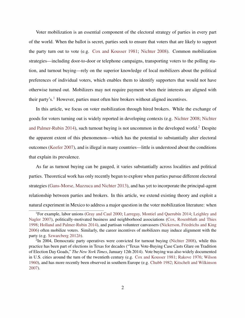
determining local vote outcomes. In some areas, parties request lists of voters whom the broker

intends to bring to the polling station. These lists can be cross-checked using the “bingo system”,

whereby party representatives at the polling station on election day with access to the list of citizens

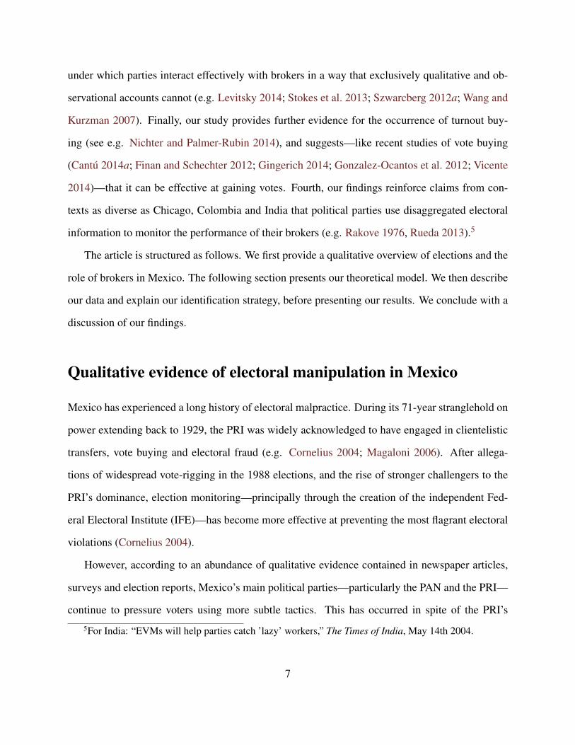
that voted compare the two lists (Mercado 2013). Figure 1 depicts an example of such a list

12In Argentina and Paraguay, respectively, Stokes et al. (2013) and Finan and Schechter (2012) providesurvey evidence indicating that brokers possess sufficient information to target voters that they expect toreciprocate or favor a given party. More qualitative work also supports the importance of reciprocity (Auyero2000) and broker centrality in local networks (Levitsky 2014; Szwarcberg 2012a).

13Szwarcberg (2012b) points to a similar logic in Argentina, where local brokers are aspiring politicianswho learn about the preferences of local voters. Brokers in Argentina appear to differ from Mexican brokersin that they are more interested in rising in the party hierarchy.

10

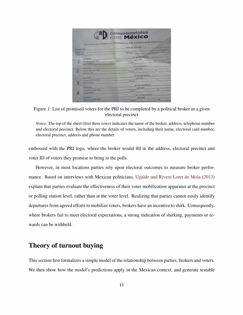
Figure 1: List of promised voters for the PRI to be completed by a political broker in a givenelectoral precinct

Notes: The top of the sheet (first three rows) indicates the name of the broker, address, telephone numberand electoral precinct. Below this are the details of voters, including their name, electoral card number,electoral precinct, address and phone number.

embossed with the PRI logo, where the broker would fill in the address, electoral precinct and

voter ID of voters they promise to bring to the polls.

However, in most locations parties rely upon electoral outcomes to measure broker perfor-

mance. Based on interviews with Mexican politicians, Ugalde and Rivera Loret de Mola (2013)

explain that parties evaluate the effectiveness of their voter mobilization apparatus at the precinct

or polling station level, rather than at the voter level. Realizing that parties cannot easily identify

departures from agreed efforts to mobilize voters, brokers have an incentive to shirk. Consequently,

where brokers fail to meet electoral expectations, a strong indication of shirking, payments or re-

wards can be withheld.

Theory of turnout buying

This section first formalizes a simple model of the relationship between parties, brokers and voters.

We then show how the model’s predictions apply in the Mexican context, and generate testable

11

hypotheses for our empirical analysis.

Formal model

Our model examines turnout buying by political parties using brokers at the electoral precinct

level. The key feature of the model is the moral hazard problem faced by political parties: parties

hire political brokers with the local knowledge required to mobilize favorable local voters, but

cannot always effectively monitor the effort exerted by political brokers in this task. Where parties

are better able to monitor brokers, they can generate more electoral support by engaging in more

extensive turnout buying. The second main feature of the model is that voters’ political preferences

and costs of turning out, as well as the cost of compensating brokers, vary with their distance

from the polling station. Depending on the location of their supporters, parties face differential

incentives to use brokers to mobilize voters facing high costs of turning out.

Setup

Consider a country containing N electoral precincts. At each electoral precinct there exists a con-

tinuum of voters, whose mass we normalize to unity. Electoral precincts differ in the distance

d > 0 that voters must travel to their polling station. For simplicity, all voters at a given polling

station travel the same distance.14 Importantly, electoral precincts also differ in the probability

p ∈ (0,1) that political parties can perfectly infer the behavior of their broker. Although parties

never fully observe broker behavior in practice, this simplifying assumption captures our main

point that in some precincts parties are more capable of reliably inferring broker actions from elec-

toral returns.15 Without loss of generality, we consider an electoral precinct defined by distance d

14We obtain very similar results if there is a distribution of voters because d can be thought of as theaverage voter.

15The electoral signal of broker performance could be modeled in a more complex manner, but theessence of the model is the same. For example, electoral outcomes could represent a noisy signal of bro-ker effort (Bolton and Dewatripont 2005: ch. 4). In that case, receiving multiple signals of performanceprovides the party with clear information about the broker’s effort level and can condition a broker’s wage

12

and probability p of observing broker effort.

Parties. We consider two political parties i = A,B competing for votes in each electoral

precinct. Parties maximize their vote share Πi in the precinct.16 However, although parties are

aware of their underlying support in any given precinct, they cannot themselves identify which

supporters to mobilize. Party i thus chooses an effort-wage contract (ei, wi) to induce a single bro-

ker to exert effort ei ∈ [0,1] to mobilize voters that favor party i. If the party observes the broker’s

effort and the broker complied with the agreed effort level, such that ei≥ ei, then she receives wage

wi; if the broker is found to not have complied with the agreed effort level, then she receives no

payment.17 If the party cannot observe ei, the broker receives wage wi.

Brokers. Political brokers enjoy an informational advantage over political parties: brokers

can identify the individual voters in their electoral precinct that would vote for party i if they

turned out.18 To keep the model tractable, we assume that brokers cannot discriminate between

voters by their likelihood of turning out to vote, and thus exert effort ei equally across voters that

would vote for party i.19 This simplification is also empirically plausible because brokers are not

always completely aware of individual costs of voting, or cannot exclude specific voters when

mobilizing large groups, while voters that always turn out may defect if they do not receive gifts

from their preferred party (Diaz-Cayeros, Estevez and Magaloni forthcoming; Nichter and Peress

2014). Furthermore, to focus on the moral hazard dimension of the problem, we assume all brokers

on the electoral outcome accordingly. Larreguy (2013) and Gingerich and Medina (2013) model signalextraction in similar contexts to ours.

16If parties instead maximized their probability of winning districts (or the Presidency) or a legislativemajority, the implications of our model are unchanged. Accordingly, parties maximize precinct vote sharefor simplicity.

17Brokers have limited liability in that parties cannot punish brokers beyond refusing to pay their wageafter observing ei < ei. We assume parties have resolved the commitment problem of paying the broker forsatisfactory performance. It is easy to rationalize this by considering repeated interactions between brokersand parties across elections. Stokes (2005) shows how this can occur between parties and voters.

18Although there is good evidence that brokers are well informed about voter preferences (see Finan andSchechter 2012; Stokes et al. 2013), this is a strong assumption. However, the logic of our model onlyrequires that brokers are better informed about vote intentions than political parties.

19We focus on the simple case without loss of intuition because targeting specific voters would producequalitatively similar results at the cost of unnecessarily complicating the model.

13

are equally effective at mobilizing voters.20

However, exerting effort ei—which could constitute calling in favors, hiring coaches and drivers,

or providing material incentives to voters—entails a cost C(d,ei) =12γide2

i to the broker, where

γi > 0 is the cost parameter for mobilizing supporters of party i. Consequently, exerting no effort

is costless to brokers, while the cost of exerting additional effort is convex and increasing in d. If

brokers are not hired by political parties, we assume they receive zero utility. Conditional upon

engaging in a contract with party i, a strategy for a broker is to choose their effort level ei.

Voters. Voters in each electoral precinct differ in the ideological shock σ toward party B that

they receive.21 This ideological shock is an expressive benefit (e.g. Brennan and Hamlin 1998;

Gans-Morse, Mazzuca and Nichter 2013), such that it is only received by voters when they turn

out and vote for their preferred candidate.22 The shock is distributed over support[− 1

2ψ, 1

2ψ

],

where a large ψ > 0 implies that variation in the expressive value of voting is low, according to the

following density function (drawn independently of d at each polling station):

g(σ ;d) = ψ [1−b(d)σ ]. (1)

This distribution function formalizes our insight that the ideological shock depends upon the dis-

tance to the polling station through b(d) ∈ [−ψ ,ψ ], where b is a monotonic function.

Integrating over the distribution of ideological shocks, the expected ideological shock toward

party B, in an electoral precinct of type d, is E[σ |d] = − b(d)12ψ2 . The term b(d) represents the bias

20Since we lack the data to capture heterogeneity across brokers—something which Stokes et al. (2013)discuss in terms of the adverse selection problem—we abstract from this issue and simply assume thatbrokers are identical in our model.

21Voters’ policy utility is not included in the model because that is not the focus of this analysis. Wecould easily introduce policy utility u(i,v) for voter type v from the platform of party i. However, allowingpolicy utilities to vary across voters does not affect the insights of the model, so we effectively assumeu(A,v) = u(B,v) for all voters and focus on our main parameters of interest.

22Since an individual’s marginal effect on the probability of winning is zero with a continuum of voters,we use expressive voting to ensure non-negligible turnout (see Palfrey and Rosenthal (1985) for low turnoutin large elections).

14

in favor of party A. Party A benefits on average in electoral precincts where b(d) > 0, because

this reduces the likelihood that voters receive a pro-B ideological shock. In competitive precincts,

where b(d) = 0, the vote is split equally in expectation. To capture rural-urban divisions, we

assume b′(d) > 0 such that party A gains relatively more support vis-a-vis party B as the distance

to the polling station increases.23

Voters also face a cost of turning out to vote. We define this cost as c(d,ei) = αd(1− ei) ∈

[0, 1ψ], where α > 0 is a cost parameter. The cost of voting thus increases in the distance d to

the polling station, but this can be counteracted by broker mobilization effort ei. A strategy for

a voter receiving ideological shock σ is the decision to vote for party A, party B or not turn out:

v(d,eA,eB;σ) ∈ {A,B, /0}. Since brokers only target voters with an ideological shock toward their

party, a voter only ever receives incentives to turn out from the broker of one party.

Timing. Finally, the game proceeds as follows:

1. Parties i = A,B offer brokers a contract (ei, wi) to induce voters to turn out.

2. The ideological shock σ is realized for all voters, but is only observed by voters and brokers.

3. A broker employed by party i exerts effort ei to mobilize its voters.

4. Voting occurs according to v(d,eA,eB;σ), and eA and eB are respectively observed by parties

A and B each with probability p.

5. The election outcome and broker payment occur, and payoffs are realized.

We now proceed to identify the contracts that define the subgame perfect Nash equilibrium (SPNE)

of this game.

23This is without loss of generality in that we could equally have chosen b′(d) < 0.

15

Equilibrium

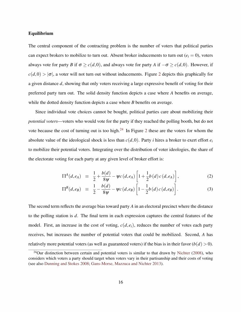
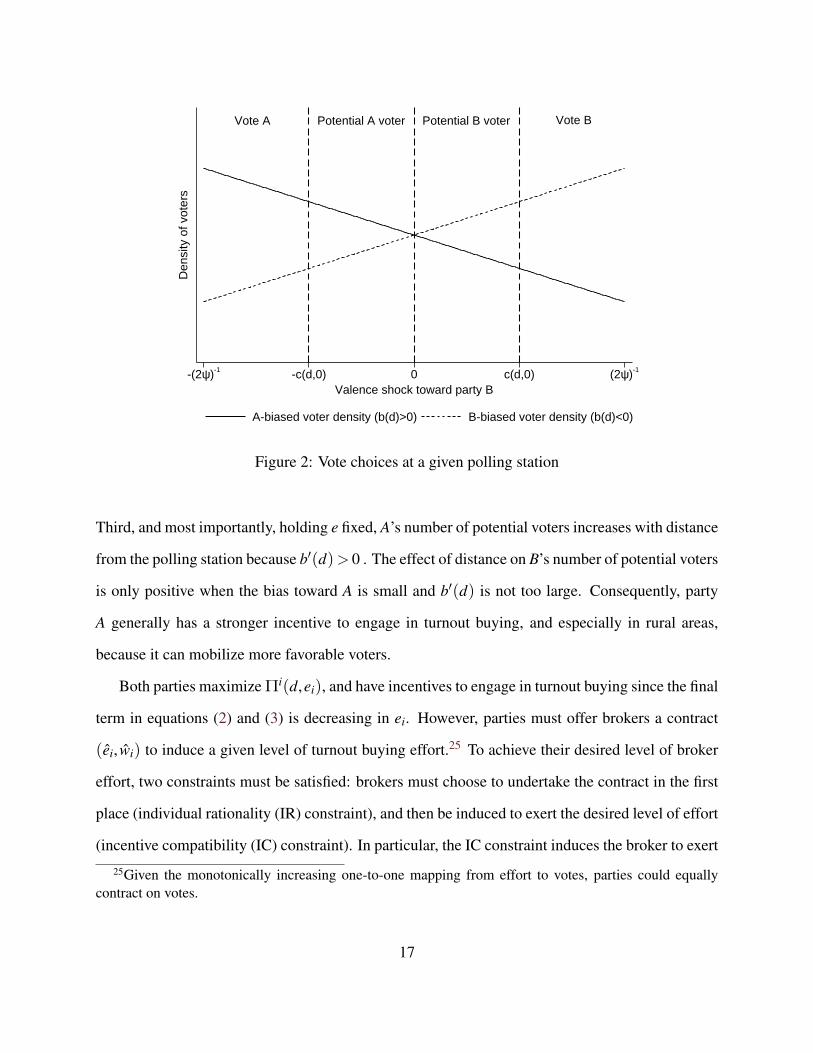
The central component of the contracting problem is the number of voters that political parties

can expect brokers to mobilize to turn out. Absent broker inducements to turn out (ei = 0), voters

always vote for party B if σ ≥ c(d,0), and always vote for party A if −σ ≥ c(d,0). However, if

c(d,0) > |σ |, a voter will not turn out without inducements. Figure 2 depicts this graphically for

a given distance d, showing that only voters receiving a large expressive benefit of voting for their

preferred party turn out. The solid density function depicts a case where A benefits on average,

while the dotted density function depicts a case where B benefits on average.

Since individual vote choices cannot be bought, political parties care about mobilizing their

potential voters—voters who would vote for the party if they reached the polling booth, but do not

vote because the cost of turning out is too high.24 In Figure 2 these are the voters for whom the

absolute value of the ideological shock is less than c(d,0). Party i hires a broker to exert effort ei

to mobilize their potential voters. Integrating over the distribution of voter ideologies, the share of

the electorate voting for each party at any given level of broker effort is:

ΠA(d,eA) ≡12+

b(d)8ψ−ψc (d,eA)

[1+

12

b (d)c (d,eA)

], (2)

ΠB(d,eB) ≡12− b(d)

8ψ−ψc (d,eB)

[1− 1

2b (d)c (d,eB)

]. (3)

The second term reflects the average bias toward party A in an electoral precinct where the distance

to the polling station is d. The final term in each expression captures the central features of the

model. First, an increase in the cost of voting, c(d,ei), reduces the number of votes each party

receives, but increases the number of potential voters that could be mobilized. Second, A has

relatively more potential voters (as well as guaranteed voters) if the bias is in their favor (b(d)> 0).

24Our distinction between certain and potential voters is similar to that drawn by Nichter (2008), whoconsiders which voters a party should target when voters vary in their partisanship and their costs of voting(see also Dunning and Stokes 2008; Gans-Morse, Mazzuca and Nichter 2013).

16

Vote A Potential A voter Potential B voter Vote B

Den

sity

of v

oter

s

-(2y)-1 -c(d,0) 0 c(d,0) (2y)-1

Valence shock toward party B

A-biased voter density (b(d)>0) B-biased voter density (b(d)<0)

Figure 2: Vote choices at a given polling station

Third, and most importantly, holding e fixed, A’s number of potential voters increases with distance

from the polling station because b′(d)> 0 . The effect of distance on B’s number of potential voters

is only positive when the bias toward A is small and b′(d) is not too large. Consequently, party

A generally has a stronger incentive to engage in turnout buying, and especially in rural areas,

because it can mobilize more favorable voters.

Both parties maximize Πi(d,ei), and have incentives to engage in turnout buying since the final

term in equations (2) and (3) is decreasing in ei. However, parties must offer brokers a contract

(ei, wi) to induce a given level of turnout buying effort.25 To achieve their desired level of broker

effort, two constraints must be satisfied: brokers must choose to undertake the contract in the first

place (individual rationality (IR) constraint), and then be induced to exert the desired level of effort

(incentive compatibility (IC) constraint). In particular, the IC constraint induces the broker to exert

25Given the monotonically increasing one-to-one mapping from effort to votes, parties could equallycontract on votes.

17

effort ei = ei at cost C(d,ei),26 rather than choose ei = 0 and receive wi if their shirking is not

caught (with probability 1− p) and receive zero when their shirking is caught (with probability p).

Party i thus solves the following program:

maxei,wi

Πi(d, ei)− wi subject to

(IC) : wi−12

γide2i ≥ (1− p)wi, (4)

(IR) : wi−12

γide2i ≥ 0.

Solving this problem leads immediately to our equilibrium result:

Proposition 1 When γA + pψα2db(d)> 0 and γB− pψα2db(d)> 0, there exists a unique SPNE

[(e∗A, w∗A), (e∗B, w∗B),e

∗A,e∗B,v∗(d,e∗A,e∗B;σ)] defined by:

e∗A = e∗A =

0 if 1+αdb(d) ≤ 0

pψα [1+αdb(d)]γA+pψα2db(d) if 1+αdb(d) > 0 and γA > pψα

1 otherwise

e∗B = e∗B =

0 if 1−αdb(d) ≤ 0

pψα [1−αdb(d)]γB−pψα2db(d) if 1−αdb(d) > 0 and γB > pψα

1 otherwise

w∗i =γide∗2i

2p,

v∗(d,e∗A,e∗B;σ) =

L if σ ≤−c(d,e∗A)

/0 if σ ∈ (−c(d,e∗A),c(d,e∗B))

R if σ ≥ c(d,e∗B)

.

26The broker does not choose ei > ei because this entails a cost without increasing their wage.

18

Equilibrium turnout is T (d,e∗A,e∗B) ≡ ∑i∈{A,B}Πi(d,e∗i ).

All proofs are in the Online Appendix.

In equilibrium, parties offer brokers a contract to just induce optimal effort. The optimal

amount of effort reflects two competing forces: the effectiveness of brokers at procuring additional

votes, which depends crucially on the number of potential voters, and the cost of effort—adjusted

for the probability of being monitored—for which the broker must be compensated for. The con-

ditions for the existence of an equilibrium, given at the beginning of Proposition 1, guarantee that

the maximization problems of both parties are well defined. An interior solution for each party

exists under two intuitive conditions provided in the proposition. First, the bias b(d) toward the

other party is never large enough that there are insufficient potential supporters of a party for it to

be able to justify the cost of hiring a broker to mobilize voters. Second, γi must be sufficiently

large to prevent a party from always mobilizing all voters.

Comparative statics

The following proposition identifies the central testable predictions of the model:

Proposition 2 In the unique SPNE identified in Proposition 1, the following comparative statics

hold at any interior solution:

1. T , eA and eB are increasing in p.

2. Let ε(d) ≡ db′(d)b(d) >−1 and γi > 2pψα . Then:

(a) There exists a dA > 0 such that the effect of p on e∗A is increasing in d for d ∈ (0,dA]

and strictly decreasing in d for d > dA.

(b) The effect of p on e∗B is decreasing in d.

19

Part 1 has a simple interpretation: increased monitoring capacity increases turnout buying by

both parties. Intuitively, this is because parties can better monitor their brokers and can therefore

more effectively threaten brokers with receiving a low wage. Consequently, parties can obtain

more turnout buying for a relatively low wage.27

The most novel predictions of the model concern the effect of distance to the polling station

on the impact of increased monitoring on turnout buying. While Part 1 of Proposition 2 shows

that greater monitoring capacity always increases turnout buying, Part 2(a) shows that this effect is

increasing in distance for party A until the distance becomes sufficiently large.28 In other words,

monitoring’s impact on party A’s turnout buying is greatest at intermediate distances. As the dis-

tance to the polling station increases, there are more favorable voters for party A to buy, both

because more rural voters favor party A and because their turnout is lower. However, the cost of

hiring a broker to mobilize distant voters becomes prohibitively large for voters living sufficiently

far from the polling station, despite their high support for party A. This non-linear prediction holds

under two conditions. First, ε(d)>−1 implies that the elasticity of bias with respect to d is never

too negative. In other words, this assumption implies that the urban-rural divide is greater than any

bias toward B. Second, γi > 2pψα implies that the cost to brokers of exerting effort relative to

the cost to voters of turning out is sufficiently large. If hiring brokers was both cheap and highly

effective, then both parties would often mobilize virtually all voters.

The final part of Proposition 2 shows that the effect of monitoring capacity on turnout buying

changes with distance very differently for party B. In particular, the increase in turnout buying due

to greater monitoring capacity is lower when voters live further from the polling station. Intuitively,

this is because party B—which does well primarily among urban voters—has fewer potential voters

to mobilize in precincts where the distance from the polling station is large, in addition to having

to pay brokers higher wages in such precincts.

27The Online Appendix shows that the effect of p on ei carries over to Πi for i = A,B.28The Online Appendix demonstrates that when the first-order effects dominate, the differential effects

of p on ei by d carry over to Πi for i = A,B.

20

Observable implications for Mexico

The theoretical model has clear predictions for our Mexican case, to which the model applies well.

Most regions of Mexico are dominated by two large parties: between 2000 and 2012, only 14% of

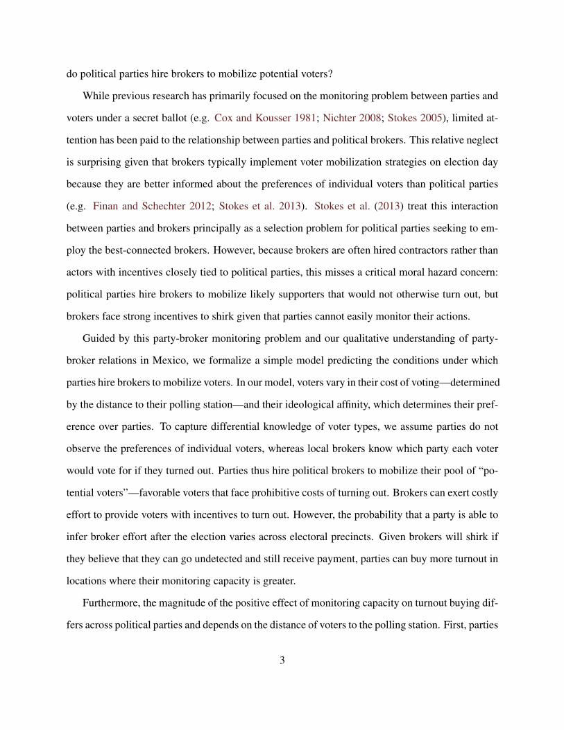
electoral precincts had a third party with more than 20% of the vote. Furthermore, as consistently

shown in U.S. studies (see Brady and McNulty 2011; Gimpel and Schuknecht 2003), Figure 3

demonstrates that polling station turnout declines with the average distance to the polling station.

Moreover, as discussed above, there is considerable qualitative evidence pointing to the importance

of local brokers in mobilizing voters for a given party at the precinct level.

A central prediction of the model is that turnout buying—captured by an increase in the total

number of votes for a party—is more prevalent where parties are more effective at monitoring their

brokers. This is because monitoring reduces the incentive for brokers to shirk. Although moni-

toring could work in a variety of ways, this article focuses on how the number of polling stations

within an electoral precinct affects turnout. In particular, we argue that a larger number of polling

stations improves monitoring capacity by producing multiple signals of broker performance.

Intuitively, parties struggle to differentiate voter-level shocks from the turnout buying effort of

their brokers when examining precinct-level electoral returns. For example, if all voters vote at a

single polling station and the party experiences electoral performance below its expectations, it is

difficult to disentangle whether this was due to a negative voter-level shock or because the broker

shirked. An additional polling station, and thus an extra signal of electoral performance, allows

parties to better differentiate random voter-level shocks that affect their vote share from broker

effort. Observing more signals of precinct-level performance always conveys more information

unless the shocks are perfectly correlated.29 For example, if voters are randomly allocated across

29To see this mathematically, compare receiving one or two signals of broker’s effort from election resultsin a given precinct. The single signal for a whole precinct has mean µ and variance σ2. When receiving twodifferent signals si, after randomly splitting voters into two polling stations, the common mean is µ/2, thevariance is σ2/4 and the covariance is ρσ2/4, where ρ is the correlation between the two signals. Then,the variance of receiving two signals, V [s1 + s2] = (1+ ρ)σ2/2, is less than σ2 provided the two signals

21

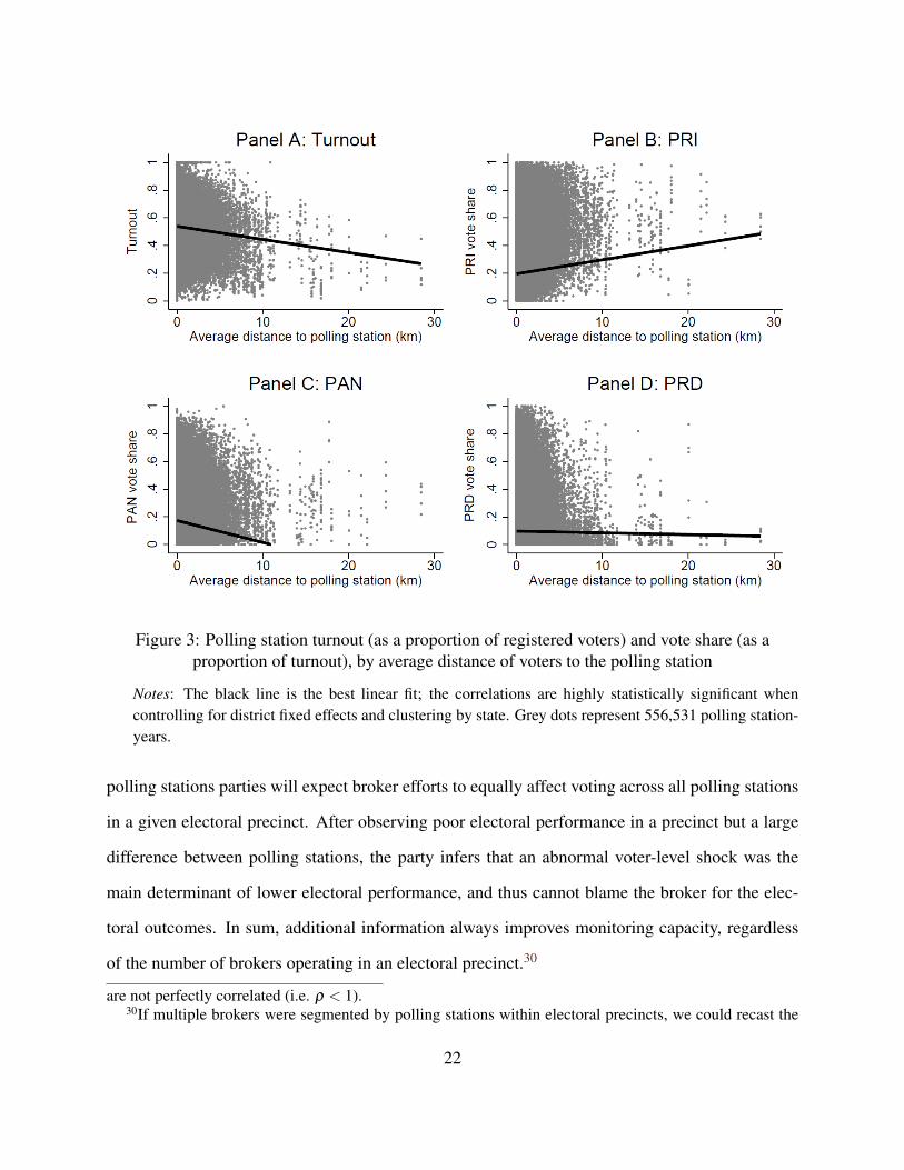
Figure 3: Polling station turnout (as a proportion of registered voters) and vote share (as aproportion of turnout), by average distance of voters to the polling station

Notes: The black line is the best linear fit; the correlations are highly statistically significant whencontrolling for district fixed effects and clustering by state. Grey dots represent 556,531 polling station-years.

polling stations parties will expect broker efforts to equally affect voting across all polling stations

in a given electoral precinct. After observing poor electoral performance in a precinct but a large

difference between polling stations, the party infers that an abnormal voter-level shock was the

main determinant of lower electoral performance, and thus cannot blame the broker for the elec-

toral outcomes. In sum, additional information always improves monitoring capacity, regardless

of the number of brokers operating in an electoral precinct.30

are not perfectly correlated (i.e. ρ < 1).30If multiple brokers were segmented by polling stations within electoral precincts, we could recast the

22

Given that we cannot observe broker effort empirically, we focus on the implications for elec-

toral outcomes. We therefore hypothesize that:

H1. Turnout and the share of votes for each political party (both as a proportion of registered vot-

ers) increases in the number of polling stations (monitoring capacity) in an electoral precinct.

Mexican politics is also defined by a rural-urban divide. The PRD and especially the PAN

are best-supported in more urban areas, among educated voters, and where clientelistic ties are

weaker. Conversely, the PRI continues to win a large proportion of more rural voters. Figure 3

illustrates these relationships, and clearly indicates that b′(d) > 0 generally holds (where the PRI

can be regarded as party A and the PAN or PRD as party B). In some southern areas where the PAN

and PRD are locally dominant, the rural-urban division is less salient. Accordingly, b′(d) ≈ 0 and

any interaction between distance and turnout buying should be weaker. In this case, we expect the

effect of monitoring to decline with distance or not depend on distance. Combining these insights

with the second part of Proposition 2, we only expect the effect of monitoring on turnout buying

to depend non-linearly on distance for the PRI:

H2. The effect of an improvement in monitoring capacity on the PRI vote share (as a proportion

of registered voters) will first increase in distance from the polling station before decreasing.

The effect of an improvement in monitoring capacity on the PAN and PRD vote share will

instead decrease or exhibit no relationship with distance.

Empirical design

This section first describes the data used to test the hypotheses derived above. We then explain

how we exploit a discontinuity in the number of polling stations in an electoral precinct to estimate

problem as one of “moral hazard in teams”. In that case, polling station level data is a powerful toolfor ascertaining relative performance (Holmstrom 1982). Given voters are assigned to polling stations bysurname (see below), this type of separation is very unlikely.

23

the effects of monitoring on turnout buying. Given that we cannot directly observe turnout buying,

we also examine heterogeneous effects by distance to the polling station to ensure that our findings

are consistent with the monitoring effects predicted by the model in ways that cannot be explained

by alternative theories.

Data

Mexico’s 300 electoral districts are divided into around 67,000 electoral precincts. These, as will

be explained in more detail below, are in turn composed of polling stations. The average precinct

contains 1.97 polling stations. The IFE has collected detailed polling station level data since 2000,

including the coordinates of polling stations for recent election years. We use this data to analyze

polling station electoral returns for the 2000, 2003, 2006, 2009 and 2012 national legislative elec-

tions (excluding the Federal District). Combined, this produces a maximum sample of 561,256

polling stations.31 Detailed variable definitions and summary statistics are provided in the Online

Appendix.

Dependent variables

We use two main measures of voting behavior. We first measure polling station Turnout as a

proportion of the total number of voters registered at a given polling station. Turnout includes all

votes for political parties or coalitions, including null votes and non-registered votes. To measure

the beneficiaries of increased turnout, we measure PAN/PRD/PRI vote share as the number of

votes for the party as a proportion of the total number of registered voters. By not conditioning on

turnout, this outcome is independent of the mobilization efforts of other political parties.

31In our analysis, we restrict attention to the casilla basica and casilla contigua polling stations thatare relevant for the electoral rule we exploit. Less than 1% of polling stations are special or extraordinarypolling stations, which include temporary residents or were created to address challenging sociocultural orgeographic circumstances (see Cantu 2014b). Due to the existence of such polling stations, the electoralrule for splitting polling stations can be violated in certain precincts. We remove all such polling stations,and subtract the number of voters registered at such polling stations from the precinct totals.

24

Independent variables

To capture the ability of political parties to monitor their brokers, we measure the Number of

polling stations in a given electoral precinct. Polling stations may contain up to 750 registered

voters, while the number of registered voters in a precinct will play a central role in determining the

number of voters per polling station (see below). With the formation of the IFE in 1990, precincts

were redrawn to contain 750 voters. Demographic changes have since caused this number to

change in some precincts.

To test the heterogeneous effects in H2, we computed the average Distance (in kilometers) of

voters to their polling station. The average distance entailed calculating the electorate-weighted

distance to the polling station among the set of registered voters in each electoral precinct using

locality-level population data provided by IFE.32 Since all the polling stations in a given precinct

in our sample are located in the same place, and we cannot distinguish the geographic distribution

of voters registered at different polling stations within an electoral precinct, the weighted distance

varies by precinct rather than polling station. Polling stations are almost invariably located in the

largest locality in the precinct, and our measure is thus strongly correlated with population density

and geographic area.33 The average distance to the polling station is 0.2 kilometers.

Identification strategy

In order to identify the effects of changes in monitoring incentives on turnout buying, we lever-

age exogenous variation in the number of polling stations in an electoral precinct—and thus the

capacity of political parties to monitor their brokers—that arises from Mexico’s electoral rules.

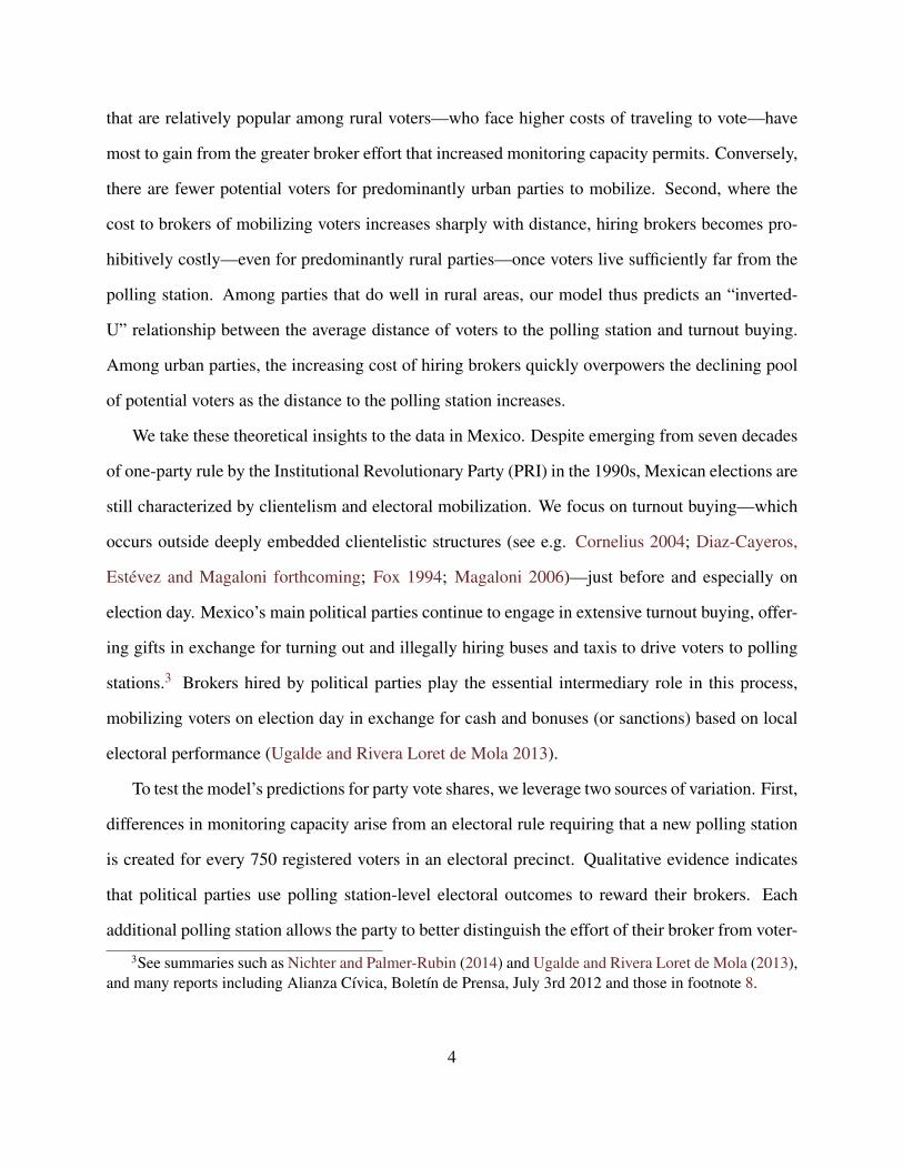
Specifically, once the registered electorate in the precinct exceeds 750 (or any such multiple) due

32Due to the difficulties of matching localities to polling station coordinates, we only use the voter geo-graphic distributions and polling station coordinates for 2012. While relatively few suburban precincts havesplit into new precincts, we restrict our sample to those that have not changed during our period of analysis.

33The correlations between weighted distance, population density (log), and area (log) in the full sampleare -0.52 and 0.58 respectively.

25

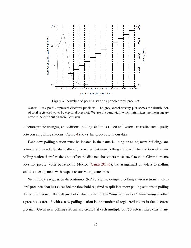
Figure 4: Number of polling stations per electoral precinct

Notes: Black points represent electoral precincts. The grey kernel density plot shows the distributionof total registered voter by electoral precinct. We use the bandwidth which minimizes the mean squareerror if the distribution were Gaussian.

to demographic changes, an additional polling station is added and voters are reallocated equally

between all polling stations. Figure 4 shows this procedure in our data.

Each new polling station must be located in the same building or an adjacent building, and

voters are divided alphabetically (by surname) between polling stations. The addition of a new

polling station therefore does not affect the distance that voters must travel to vote. Given surname

does not predict voter behavior in Mexico (Cantu 2014b), the assignment of voters to polling

stations is exogenous with respect to our voting outcomes.

We employ a regression discontinuity (RD) design to compare polling station returns in elec-

toral precincts that just exceeded the threshold required to split into more polling stations to polling

stations in precincts that fell just below the threshold. The “running variable” determining whether

a precinct is treated with a new polling station is the number of registered voters in the electoral

precinct. Given new polling stations are created at each multiple of 750 voters, there exist many

26

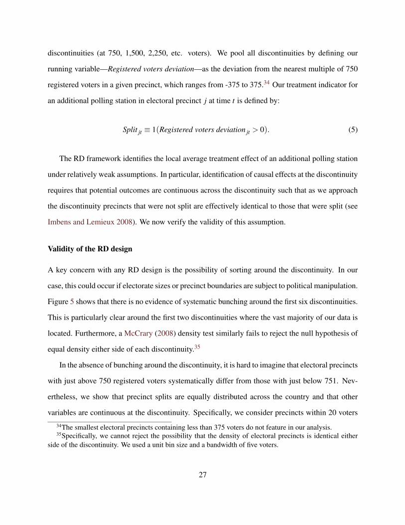
discontinuities (at 750, 1,500, 2,250, etc. voters). We pool all discontinuities by defining our

running variable—Registered voters deviation—as the deviation from the nearest multiple of 750

registered voters in a given precinct, which ranges from -375 to 375.34 Our treatment indicator for

an additional polling station in electoral precinct j at time t is defined by:

Split jt ≡ 1(Registered voters deviation jt > 0). (5)

The RD framework identifies the local average treatment effect of an additional polling station

under relatively weak assumptions. In particular, identification of causal effects at the discontinuity

requires that potential outcomes are continuous across the discontinuity such that as we approach

the discontinuity precincts that were not split are effectively identical to those that were split (see

Imbens and Lemieux 2008). We now verify the validity of this assumption.

Validity of the RD design

A key concern with any RD design is the possibility of sorting around the discontinuity. In our

case, this could occur if electorate sizes or precinct boundaries are subject to political manipulation.

Figure 5 shows that there is no evidence of systematic bunching around the first six discontinuities.

This is particularly clear around the first two discontinuities where the vast majority of our data is

located. Furthermore, a McCrary (2008) density test similarly fails to reject the null hypothesis of

equal density either side of each discontinuity.35

In the absence of bunching around the discontinuity, it is hard to imagine that electoral precincts

with just above 750 registered voters systematically differ from those with just below 751. Nev-

ertheless, we show that precinct splits are equally distributed across the country and that other

variables are continuous at the discontinuity. Specifically, we consider precincts within 20 voters

34The smallest electoral precincts containing less than 375 voters do not feature in our analysis.35Specifically, we cannot reject the possibility that the density of electoral precincts is identical either

side of the discontinuity. We used a unit bin size and a bandwidth of five voters.

27

Tabl

e1:

Bal

ance

chec

ks—

split

ting

polli

ngst

atio

nsan

dpo

litic

al,e

cono

mic

and

dem

ogra

phic

char

acte

rist

ics

ofel

ecto

ralp

reci

ncts

(1)

(2)

(3)

(4)

(5)

(6)

(7)

(8)

PRI

PAN

PRD

Are

aVo

ter

Dis

tanc

eSh

are

Shar

evo

tesh

are

vote

shar

evo

tesh

are

(log

)de

nsity

topo

lling

econ

omic

ally

empl

oyed

(lag

)(l

ag)

(lag

)st

atio

nac

tive

Split

0.00

190.

0013

-0.0

013

-0.0

080

-74.

9247

-0.0

123

-0.0

024*

**-0

.000

2(0

.001

4)(0

.001

3)(0

.001

2)(0

.024

5)(6

8.73

63)

(0.0

119)

(0.0

008)

(0.0

005)

Obs

erva

tions

22,6

7422

,674

22,6

7424

,406

24,4

0627

,417

27,4

5827

,458

(9)

(10)

(11)

(12)

(13)

(14)

(15)

(16)

Shar

eSh

are

Inco

mpl

ete

Com

plet

eIn

com

plet

eC

ompl

ete

Shar

eSh

are

med

ical

illite

rate

prim

ary

prim

ary

seco

ndar

yse

cond

ary

owns

basi

cin

sura

nce

scho

olsc

hool

scho

olsc

hool

hous

eam

eniti

es

Split

-0.0

023

0.00

010.

0018

-0.0

010

-0.0

016

-0.0

018

0.00

00-0

.000

5(0

.001

8)(0

.000

6)(0

.003

4)(0

.002

6)(0

.001

8)(0

.001

7)(0

.001

5)(0

.003

5)

Obs

erva

tions

27,4

5527

,455

27,4

5527

,455

27,4

5527

,455

27,4

6027

,460

(17)

(18)

(19)

(20)

(21)

(22)

(23)

(24)

Shar

eSh

are

Shar

eSh

are

Shar

eSh

are

Shar

eSh

are

with

with

with

was

hing

with

with

with

cell

with

radi

oT

Vfr

idge

mac

hine

car

tele

phon

eph

one

inte

rnet

Split

-0.0

037*

*-0

.000

5-0

.001

7-0

.003

6-0

.003

3-0

.003

0-0

.007

5**

-0.0

017

(0.0

016)

(0.0

013)

(0.0

022)

(0.0

025)

(0.0

031)

(0.0

031)

(0.0

034)

(0.0

034)

Obs

erva

tions

27,4

6027

,460

27,4

6027

,460

27,4

6027

,460

27,4

6027

,460

Not

es:

Eac

hco

effic

ient

estim

ates

the

effe

ctof

split

ting

apo

lling

stat

ion

ona

pre-

trea

tmen

tou

tcom

e,an

dis

estim

ated

sepa

rate

lyfr

oman

OL

Sre

gres

sion

incl

udin

gdi

stri

ct-y

ear

fixed

effe

cts.

Thi

sis

the

form

ofou

rm

ain

spec

ifica

tions

.B

lock

-boo

tstr

appe

dst

anda

rder

rors

are

clus

tere

dby

stat

e(1

,000

resa

mpl

es).

Such

spec

ifica

tions

are

iden

tical

toou

rm

ain

empi

rica

lana

lysi

s.*

deno

tes

p<

0.1,

**de

note

sp<

0.05

,***

deno

tes

p<

0.01

.

28

010

020

030

0

Fre

quen

cy730 740 750 760 770

Number of registered voters

Panel A: 750-voter discontinuity

050

100

150

Fre

quen

cy

1480 1490 1500 1510 1520

Number of registered voters

Panel B: 1500-voter discontinuity

010

2030

Fre

quen

cy

2230 2240 2250 2260 2270

Number of registered voters

Panel C: 2250-voter discontinuity

02

46

810

Fre

quen

cy

2980 2990 3000 3010 3020

Number of registered voters

Panel D: 3000-voter discontinuity

01

23

45

Fre

quen

cy

3730 3740 3750 3760 3770

Number of registered voters

Panel E: 3750-voter discontinuity

01

23

4

Fre

quen

cy4480 4490 4500 4510 4520

Number of registered voters

Panel F: 4500-voter discontinuity

Figure 5: Histograms of the number of electoral precincts either side of the discontinuity

of being split to precincts that exceeded a multiple of 750 by less than 20 voters. This yields a

sample of 26,697 polling stations from 13,452 precincts that were close to being split at a given

election. As depicted in Figure 6, the 10,970 different electoral precincts that are included in our

analysis at least once are equally distributed across the country.36

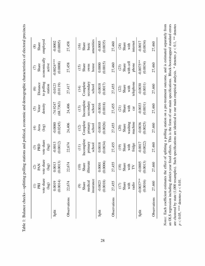
Table 1 presents 24 observable political, economic and demographic characteristics of these

polling stations, and shows that treated and control units are well balanced across these variables.37

The few differences are extremely small relative to their sample means. Nevertheless, we include

all variables as controls as a robustness check in the Online Appendix. Throughout we include

district-year fixed effects to ensure that our results cannot be driven by any race, district or state-

36As shown in the Online Appendix, the share of polling stations from each state in the discontinuitysample almost exactly reflects the population distribution.

37The Online Appendix plots these variables from contemporaneous IFE electoral data and the 2010Census as a function of our running variable, and similarly supports continuity across the discontinuity.Census data for earlier years is not available at the precinct level.

29

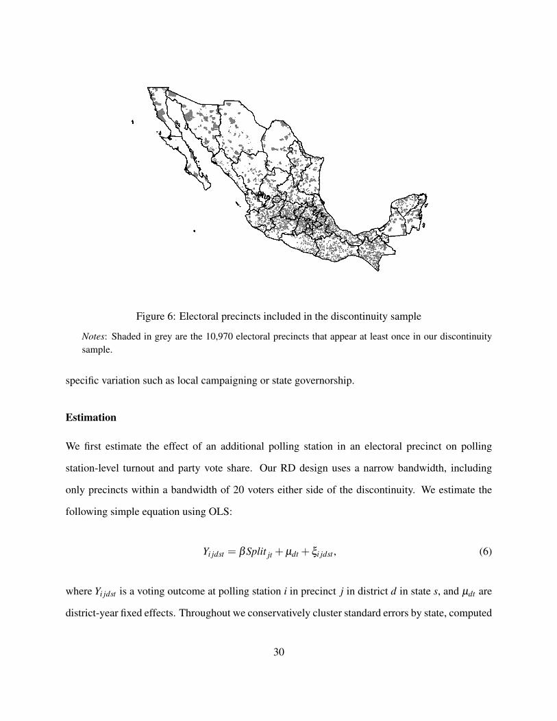
Figure 6: Electoral precincts included in the discontinuity sample

Notes: Shaded in grey are the 10,970 electoral precincts that appear at least once in our discontinuitysample.

specific variation such as local campaigning or state governorship.

Estimation

We first estimate the effect of an additional polling station in an electoral precinct on polling

station-level turnout and party vote share. Our RD design uses a narrow bandwidth, including

only precincts within a bandwidth of 20 voters either side of the discontinuity. We estimate the

following simple equation using OLS:

Yi jdst = βSplit jt + µdt + ξi jdst , (6)

where Yi jdst is a voting outcome at polling station i in precinct j in district d in state s, and µdt are

district-year fixed effects. Throughout we conservatively cluster standard errors by state, computed

30

using a block bootstrap based on 1,000 resamples. We show below that our results are insensitive

to the choice of bandwidth and robust to including trends via a local linear regression.

To test the distance-specific predictions of the theory, we also estimate the following quadratic

interaction specifications:

Yi jdst = βSplit jt +2

∑k=1

τ0kDistancekj +

2

∑k=1

τ1k

(Split jt×Distancek

j

)+ µdt + ξi jdst , (7)

where Distancekj measures the average distance of voters to the polling station(s) in precinct j. We

use a quadratic interaction for simplicity, but obtain similar results using less parametric specifica-

tions. To demonstrate that distance is not simply proxying for another variable, we also control for

interactions with our balancing variables as a robustness check.

Results

Our results provide support for the theoretical model, and thus for the presence of greater turnout

buying in areas where parties can better monitor the performance of their brokers. We first show

a jump in turnout and PRI and PAN vote shares at the discontinuity determining the creation of

a new polling station. Distinguishing our monitoring mechanism from potentially confounding

explanations, we then show that the effect of an additional polling station increases and then de-

creases with distance—but only for the PRI. Finally, we show that our results are highly robust

across a wide range of alternative specifications.

Average effects of an additional polling station

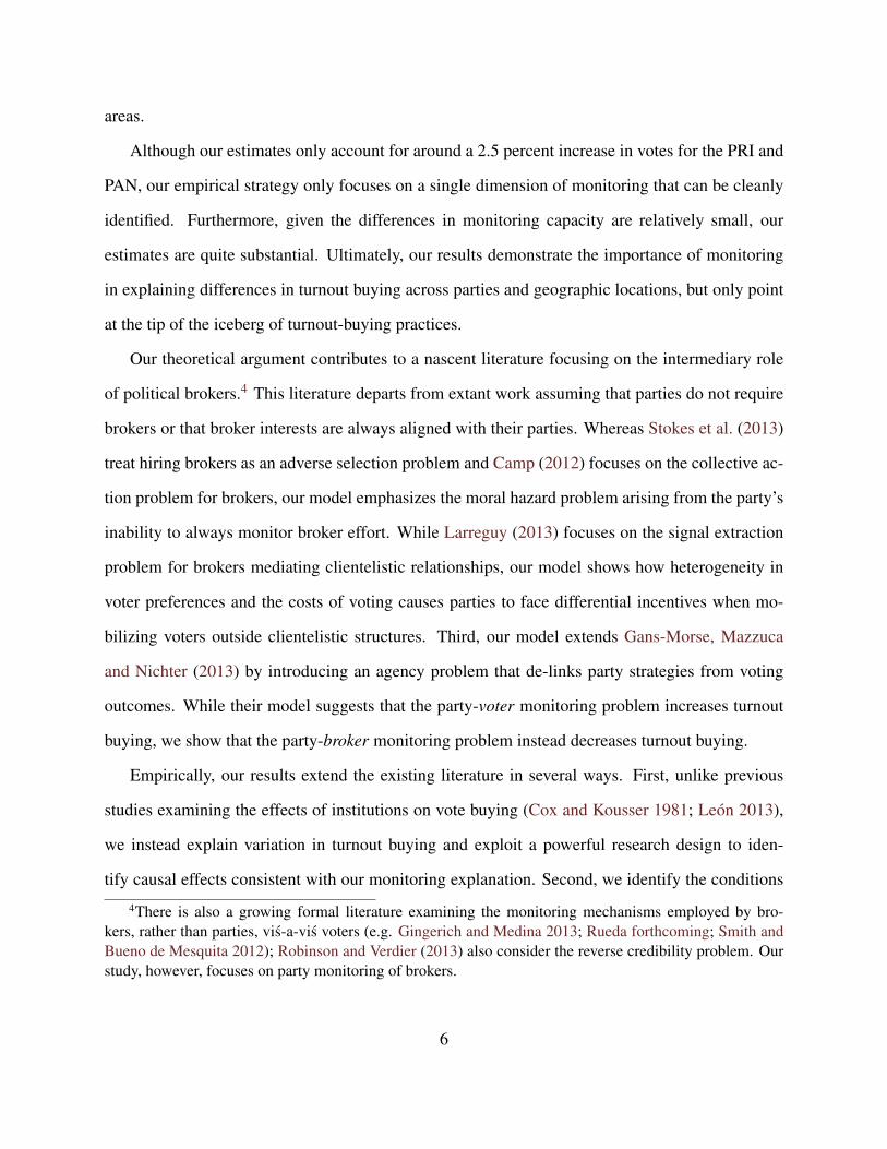
Before estimating equation (6), we first depict our variation graphically. Panel A of Figure 7

shows a jump in turnout of nearly one percentage point once a polling station is split. Panels B-D

examine party vote share, and suggest that the PRI—traditionally Mexico’s most clientelistic and

31

.525

.53

.535

.54

.545

.55

Tur

nout

-400 -200 0 200 400

Number of voters from splitting

Panel A: turnout

.185

.19

.195

.2.2

05

PR

I vot

e sh

are

-400 -200 0 200 400

Number of voters from splitting

Panel B: PRI.1

6.1

65.1

7.1

75.1

8

PA

N v

ote

shar

e

-400 -200 0 200 400

Number of voters from splitting

Panel C: PAN

.09

.095

.1.1

05

PR

D v

ote

shar

e

-400 -200 0 200 400

Number of voters from splitting

Panel D: PRD

Figure 7: The effect of splitting polling stations on turnout and party vote share

Notes: Points in each graph represent the mean outcome for bins of registered voters of size five. Theblack line is the best linear fit either side of the discontinuity.

fraudulent political party—and the PAN—which held the Presidency between 2000 and 2012—are

the principal beneficiaries of adding a new polling station. Conversely, there is little evidence that

the PRD, which has regularly denounced vote buying and likely inherited the weakest political

machines from the PRI, experienced a change in their vote share. We now test these relationships

more formally.

The regression results in Table 2 support the changes identified in Figure 7. Column (1) shows

that, on average, splitting a precinct increases polling station turnout by 0.85 percentage points.

Given average turnout is just over 50%, this represents nearly a two percent increase in the propor-

32

tion turning out to vote. This finding is consistent with our argument (in H1) that parties are better

able to monitor their brokers in electoral precincts with more polling stations.

Columns (2)-(4) examine changes in vote share by party. The results reiterate that the PRI and

PAN are the main beneficiaries, respectively increasing the number of votes they receive in the

average precinct by 0.45 and 0.41 percentage points. This represents a 2.5 percent increase in both

party’s vote share. The results imply that turnout buying is most prevalent by the PRI, although the

PAN is engaged in almost as much turnout buying. Given that the PAN and PRI were the largest

parties between 2000 and 2012, on average, they stood to gain most votes from buying turnout;

this is consistent with the predictions of our model.

Our findings for the PRI are supported by our accounts above and the existing literature. While

apparently inconsistent with the literature on clientelism that highlights that clientelistic exchanges

are concentrated among poor voters (Diaz-Cayeros, Estevez and Magaloni 2007, Weitz-Shapiro

2012), the results for the PAN—traditionally associated with middle-class voters—are probably

driven by poor voters in urban and suburban areas. Furthermore, some accounts indicate that some

PAN mayors pay taxi drivers for sticking the PAN logo in their cars and driving voters to the polls.

However, there is no evidence of PRD turnout buying. The estimate in column (4), which is

precisely estimated, indicates that an additional polling station does not increase the vote share

of the PRD. The Online Appendix also confirms that even in states with a PRD governor, where

turnout buying is likely to be most prevalent, there is no evidence that an additional polling sta-

tion increases PRD turnout.38 While consistent with the PRD’s campaigning, this finding might

be counter intuitive since the PRD is known for endorsing former PRI candidates that bring their

political machines with them (Garrido de Sierra 2013a,b, Langston 2012). A possible explana-

tion is that those candidates switching to the PRD were those with the weakest machines. Gar-

rido de Sierra (2013a) points out that defectors were often disgruntled PRI members who decided

to leave the party after not being nominated as candidates, suggesting that they faced worse elec-

38Focusing on only Guerrero and Michoacan, there is also no evidence of PRD turnout buying.

33

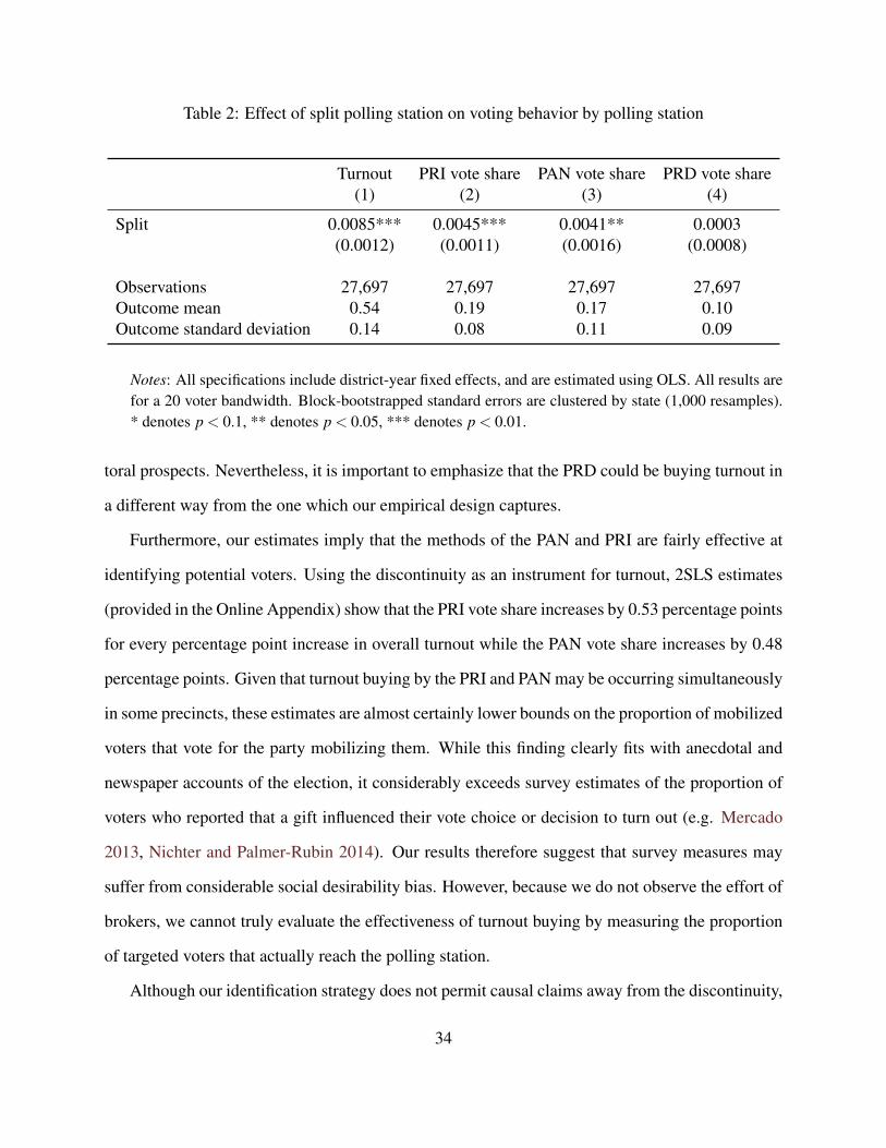
Table 2: Effect of split polling station on voting behavior by polling station

Turnout PRI vote share PAN vote share PRD vote share(1) (2) (3) (4)

Split 0.0085*** 0.0045*** 0.0041** 0.0003(0.0012) (0.0011) (0.0016) (0.0008)

Observations 27,697 27,697 27,697 27,697Outcome mean 0.54 0.19 0.17 0.10Outcome standard deviation 0.14 0.08 0.11 0.09

Notes: All specifications include district-year fixed effects, and are estimated using OLS. All results arefor a 20 voter bandwidth. Block-bootstrapped standard errors are clustered by state (1,000 resamples).* denotes p < 0.1, ** denotes p < 0.05, *** denotes p < 0.01.

toral prospects. Nevertheless, it is important to emphasize that the PRD could be buying turnout in

a different way from the one which our empirical design captures.

Furthermore, our estimates imply that the methods of the PAN and PRI are fairly effective at

identifying potential voters. Using the discontinuity as an instrument for turnout, 2SLS estimates

(provided in the Online Appendix) show that the PRI vote share increases by 0.53 percentage points

for every percentage point increase in overall turnout while the PAN vote share increases by 0.48

percentage points. Given that turnout buying by the PRI and PAN may be occurring simultaneously

in some precincts, these estimates are almost certainly lower bounds on the proportion of mobilized

voters that vote for the party mobilizing them. While this finding clearly fits with anecdotal and

newspaper accounts of the election, it considerably exceeds survey estimates of the proportion of

voters who reported that a gift influenced their vote choice or decision to turn out (e.g. Mercado

2013, Nichter and Palmer-Rubin 2014). Our results therefore suggest that survey measures may

suffer from considerable social desirability bias. However, because we do not observe the effort of

brokers, we cannot truly evaluate the effectiveness of turnout buying by measuring the proportion

of targeted voters that actually reach the polling station.

Although our identification strategy does not permit causal claims away from the discontinuity,

34

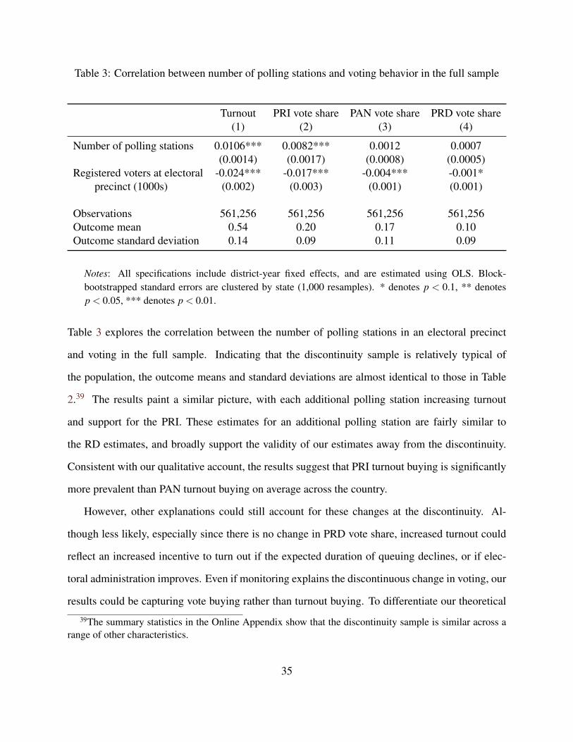
Table 3: Correlation between number of polling stations and voting behavior in the full sample

Turnout PRI vote share PAN vote share PRD vote share(1) (2) (3) (4)

Number of polling stations 0.0106*** 0.0082*** 0.0012 0.0007(0.0014) (0.0017) (0.0008) (0.0005)

Registered voters at electoral -0.024*** -0.017*** -0.004*** -0.001*precinct (1000s) (0.002) (0.003) (0.001) (0.001)

Observations 561,256 561,256 561,256 561,256Outcome mean 0.54 0.20 0.17 0.10Outcome standard deviation 0.14 0.09 0.11 0.09

Notes: All specifications include district-year fixed effects, and are estimated using OLS. Block-bootstrapped standard errors are clustered by state (1,000 resamples). * denotes p < 0.1, ** denotesp < 0.05, *** denotes p < 0.01.

Table 3 explores the correlation between the number of polling stations in an electoral precinct

and voting in the full sample. Indicating that the discontinuity sample is relatively typical of

the population, the outcome means and standard deviations are almost identical to those in Table

2.39 The results paint a similar picture, with each additional polling station increasing turnout

and support for the PRI. These estimates for an additional polling station are fairly similar to

the RD estimates, and broadly support the validity of our estimates away from the discontinuity.

Consistent with our qualitative account, the results suggest that PRI turnout buying is significantly

more prevalent than PAN turnout buying on average across the country.

However, other explanations could still account for these changes at the discontinuity. Al-

though less likely, especially since there is no change in PRD vote share, increased turnout could

reflect an increased incentive to turn out if the expected duration of queuing declines, or if elec-

toral administration improves. Even if monitoring explains the discontinuous change in voting, our

results could be capturing vote buying rather than turnout buying. To differentiate our theoretical

39The summary statistics in the Online Appendix show that the discontinuity sample is similar across arange of other characteristics.

35

Table 4: Effect of split polling station by distance

Turnout PRI vote share PAN vote share PRD vote share(1) (2) (3) (4)

Split 0.0084*** 0.0034*** 0.0042** 0.0006(0.0014) (0.0011) (0.0018) (0.0011)

Distance -0.0067 0.0058 -0.0089*** -0.0017(0.0049) (0.0036) (0.0032) (0.0020)

Distance squared -0.0003 -0.0006 0.0003 0.0000(0.0007) (0.0007) (0.0006) (0.0003)

Split × Distance 0.0014 0.0110*** -0.0035 -0.0002(0.0047) (0.0036) (0.0028) (0.0031)

Split × Distance squared -0.0009 -0.0030** 0.0010* -0.0005(0.0014) (0.0013) (0.0006) (0.0007)

Observations 27,420 27,420 27,420 27,420

Notes: All specifications include district-year fixed effects, and are estimated with OLS. All results arefor a 20 voter bandwidth. Block-bootstrapped standard errors are clustered by state (1,000 re-samples).Locality-weighted distance to the polling station was unavailable for 347 electoral precincts. * denotesp < 0.1, ** denotes p < 0.05, *** denotes p < 0.01.

explanation from such alternative interpretations, we test the heterogeneous effects by distance

exclusively predicted by our turnout buying model.

Heterogeneous effects of additional polling stations by distance

To test our hypothesis that increased monitoring capacity only translates into turnout buying when

there exist potential voters that can be bought at relatively low cost, we estimate equation (7). The

first, fourth and fifth rows in Table 4 show the differential effects of an additional polling station

by average distance to the polling station: the first coefficient identifies the effect of an additional

polling station in urban areas where the distance to the polling station is essentially zero, while the

two interaction terms (fourth and fifth coefficients) allow for the effect of splitting a polling station

to vary with distance.

36

-.06

-.04

-.02

0.0

2M

argi

nal e

ffect

of s

plitt

ing

on P

RI v

ote

shar

e

0 1 2 3 4 5Average distance to polling station (km)

Figure 8: Marginal effect of splitting polling stations on PRI vote share by distance (with 95%confidence interval)

We find non-linear effects of monitoring capacity in line with H2. The interaction estimates

in column (2) show that splitting a polling station particularly increases the PRI vote share in

locations where voters are not too close but not too far from the polling station. Figure 8 illustrates

the result graphically, showing that the effect of an additional polling station is maximized where

the average voter lives around 1.75km from the polling station.40 Where the effect of monitoring is

largest, the PRI vote share increases by nearly 1.5 percentage points, or nearly 10 percent of their

total vote. These results for the PRI are consistent with our theoretical claim that the average effect

at the discontinuity is picking up differences in monitoring capacity, rather than any other change

associated with new polling stations.

Conversely, column (3) shows that the benefits of splitting polling stations for the PAN operate

very differently. Comparing the estimates in the first row, we find that the PAN benefits slightly

more from turnout buying than the PRI in the most urban areas where a polling station serves only

40We also defined indicators for different distances and found similar results, suggesting that the moni-toring effect is largest when the distance from the polling station is around 1km on average.

37

one locality. Unlike for the PRI, but consistent with H2, this effect does not increase with distance.

Rather, the PAN vote share generally declines with distance: although the linear interaction with

distance is not quite significantly negative, the linear effect of distance shows there is already

a strong decline in vote share on the other side of the discontinuity. These results fit with the

differential predictions of our model across parties, suggesting that the lack of potential PAN voters

living further from polling stations means that it is not worth hiring brokers to reach these areas.

Column (4) shows no differential effects for the PRD. This is consistent with our finding above

that the PRD is not engaging in significant turnout buying of the sort captured by our identification

strategy.

These heterogeneous effects are not consistent with the most plausible alternative explanations

for the effects of an additional polling station. First, if improved electoral administration or lower

waiting time at the polling booth simply reduces the costs of turning out, the Online Appendix

shows that this should increase the vote share of all parties. However, we find no positive effect

on the PRD vote share. Furthermore, the increased number of votes for the PRI should be mono-

tonically increasing in distance, while the increased number of votes for the PAN and PRD are

expected to be monotonically decreasing in distance. Thus, the congestion explanation cannot ex-

plain the finding that the marginal effect of a new polling station on the PRI vote share decreases

in distance for a sufficiently large distance. Second, a mechanical effect driven by added electoral

officials present at the additional polling station—assuming that they would have not turned out

otherwise—could similarly explain neither why only the PRI and PAN benefit to begin with nor

why the non-linear effects with distance occur only for the PRI. Third, monitoring could be fa-

cilitating vote buying rather than turnout buying. However, vote buying would imply the reverse

relationship with distance because there are more opposition votes for the PRI to convert in the

less rural areas where more PAN and PRD voters reside. Similarly, we would expect the PAN and

PRD vote shares to increase with distance.

38

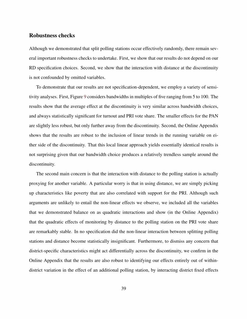
Robustness checks

Although we demonstrated that split polling stations occur effectively randomly, there remain sev-

eral important robustness checks to undertake. First, we show that our results do not depend on our

RD specification choices. Second, we show that the interaction with distance at the discontinuity

is not confounded by omitted variables.

To demonstrate that our results are not specification-dependent, we employ a variety of sensi-

tivity analyses. First, Figure 9 considers bandwidths in multiples of five ranging from 5 to 100. The

results show that the average effect at the discontinuity is very similar across bandwidth choices,

and always statistically significant for turnout and PRI vote share. The smaller effects for the PAN

are slightly less robust, but only further away from the discontinuity. Second, the Online Appendix

shows that the results are robust to the inclusion of linear trends in the running variable on ei-

ther side of the discontinuity. That this local linear approach yields essentially identical results is

not surprising given that our bandwidth choice produces a relatively trendless sample around the

discontinuity.

The second main concern is that the interaction with distance to the polling station is actually

proxying for another variable. A particular worry is that in using distance, we are simply picking

up characteristics like poverty that are also correlated with support for the PRI. Although such

arguments are unlikely to entail the non-linear effects we observe, we included all the variables

that we demonstrated balance on as quadratic interactions and show (in the Online Appendix)

that the quadratic effects of monitoring by distance to the polling station on the PRI vote share

are remarkably stable. In no specification did the non-linear interaction between splitting polling

stations and distance become statistically insignificant. Furthermore, to dismiss any concern that

district-specific characteristics might act differentially across the discontinuity, we confirm in the

Online Appendix that the results are also robust to identifying our effects entirely out of within-

district variation in the effect of an additional polling station, by interacting district fixed effects

39

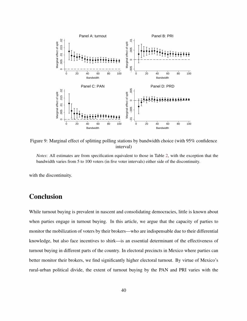
0.0

05.0

1.0

15.0

2

Mar

gina

l effe

ct o

f spl

it

0 20 40 60 80 100

Bandwidth

Panel A: turnout

-.00

50

.005

.01

Mar

gina

l effe

ct o

f spl

it

0 20 40 60 80 100

Bandwidth

Panel B: PRI

0.0

05.0

1.0

15.0

2

Mar

gina

l effe

ct o

f spl

it

0 20 40 60 80 100

Bandwidth

Panel C: PAN

-.01

-.00

50

.005

Mar

gina

l effe

ct o

f spl

it0 20 40 60 80 100

Bandwidth

Panel D: PRD

Figure 9: Marginal effect of splitting polling stations by bandwidth choice (with 95% confidenceinterval)

Notes: All estimates are from specification equivalent to those in Table 2, with the exception that thebandwidth varies from 5 to 100 voters (in five voter intervals) either side of the discontinuity.

with the discontinuity.

Conclusion

While turnout buying is prevalent in nascent and consolidating democracies, little is known about

when parties engage in turnout buying. In this article, we argue that the capacity of parties to

monitor the mobilization of voters by their brokers—who are indispensable due to their differential

knowledge, but also face incentives to shirk—is an essential determinant of the effectiveness of

turnout buying in different parts of the country. In electoral precincts in Mexico where parties can

better monitor their brokers, we find significantly higher electoral turnout. By virtue of Mexico’s

rural-urban political divide, the extent of turnout buying by the PAN and PRI varies with the

40

precinct-specific costs and benefits of hiring brokers. Better monitoring capacity enables turnout

buying where a party has many potential supporters who face prohibitive costs of turning out, but

less so once the costs of hiring brokers become too large to justify mobilizing an additional voter.

Our findings have important implications for understanding when parties deploy different elec-

toral strategies, and thus contribute more broadly to the politics of targeted distribution (Cox and

McCubbins 1986; Lindbeck and Weibull 1987). First, unlike the party-voter interaction that pre-

vious research has focused on, or the selection of brokers, we emphasize the role of parties moni-

toring their brokers. The empirical component of our study—the first, to our knowledge, to isolate

the causal effect of monitoring on turnout buying—shows that electoral returns provide parties

with valuable information about broker performance. Although electoral returns are an important

monitoring device, and have also been exploited in countries as diverse as Colombia, India and

the U.S., they probably only represent one of a plethora of monitoring mechanisms. Monitoring

issues are particularly relevant in the current U.S. context, where Enos and Hersh (forthcoming)

find that the Obama 2012 campaign struggled to overcome the agency problem that their activists,

who are typically ideologically extreme and unpaid, fail to convey messages designed by the party

to mobilize centrist voters.

Second, we confirm empirically the theoretical insight of Gans-Morse, Mazzuca and Nichter

(2013) that the distribution of voter preferences and costs of turning out are central in explaining

which parties engage in turnout buying in which locations. This finding buttresses the literature

demonstrating that political parties target their voter mobilization efforts strategically (e.g. Berry,

Burden and Howell 2010; Martin 2003). In addition to showing that political parties are sensitive

to these considerations, we also find that the interaction with structural features determining the

ability of parties to implement turnout buying may be just as important. In this respect our findings

dovetail with previous research showing that institutions like the secret ballot (Cox and Kousser

1981; Nichter 2008), compulsory voting (Leon 2013) and party machines (Rakove 1976; Stokes

et al. 2013) affect election day strategies.

41

The specific monitoring instrument examined in this article—additional polling stations—also

has implications for policy-makers designing electoral systems. El Salvador’s “voto residencial”

program, for example, has recently increased the number of polling stations available to voters,

while Pakistan introduced a similar reform in 2014.41 Similarly, India’s recently-introduced elec-

tronic voting machines allow parties to assess the relative contributions of their workers manning

each polling booth. Our findings highlight an important trade-off facing policy-makers seeking

to expand the number of polling stations. On the one hand, disaggregated electoral data can be

used by election observers to more effectively detect electoral fraud, while increasing the number

of polling stations may increase political participation by reducing the costs of voting. On the

other hand, our results suggest that parties can use more detailed data to buy more turnout because

they can better monitor their brokers. What is best is likely to depend on the context, although

relative ease with which these changes could be achieved is worth noting. This contrasts with

prominent accounts emphasizing the role of slow-changing structural factors like economic devel-

opment, political competition and income inequality in reducing vote buying (e.g. Stokes et al.

2013; Weitz-Shapiro 2012).

The concerns about turnout buying are premised on the assumption that it is bad for democracy.

However, its effect probably varies across contexts. To the extent that turnout buying increases the

participation of previously under-represented groups, it could be regarded as socially beneficial.

Conversely, the advantage given to some parties—especially previously dominant parties like the

PRI, who already possess the networks and resources to buy votes—may counteract the participa-

tory benefits. Our theory and evidence suggest that careful electoral design could mitigate turnout

buying –in those contexts where the negative effects of turnout buying for democracy are clear– by

recognizing where dominant parties are most likely to exploit turnout buying potential.

41“ECP to increase number of polling stations,” Dunya News, December 10th 2014.

42

References

Auyero, Javier. 2000. Poor People’s Politics: Peronist Survival Networks and the Legacy of Evita.

Duke University Press.

Berry, Christopher R., Barry C. Burden and William G. Howell. 2010. “The president and the

distribution of federal spending.” American Political Science Review 104(4):783–799.

Bolton, Patrick and Mathias Dewatripont. 2005. Contract Theory. MIT press.

Brady, Henry E. and John E. McNulty. 2011. “Turning out to vote: The costs of finding and getting

to the polling place.” American Political Science Review 105(01):115–134.

Brennan, Geoffrey and Alan Hamlin. 1998. “Expressive voting and electoral equilibrium.” Public

Choice 95(1-2):149–175.

Camp, Edwin. 2012. “Animating the Machine.” Working paper.

Cantu, Francisco. 2014a. “Groceries for Votes? Clientelistic Strategies in Mexico’s 2012 Election.”

Working paper.

Cantu, Francisco. 2014b. “Identifying Electoral Irregularities in Mexican Local Elections.” Amer-

ican Journal of Political Science 58(4):936–951.

Chubb, Judith. 1982. Patronage, Power and Poverty in Southern Italy: A Tale of Two Cities.

Cambridge University Press.

Cornelius, Wayne A. 2004. Mobilized voting in the 2000 elections: The changing efficacy of

vote buying and coercion in Mexican electoral politics. In Mexico’s Pivotal Democratic Elec-

tions: Candidates, Voters, and the Presidential Campaign of 2000, ed. Jorge I. Dominguez and

Chappell Lawson. Stanford University Press pp. 47–65.

43

Cox, Gary W., Frances M. Rosenbluth and Michael F. Thies. 1998. “Mobilization, social networks,

and turnout: Evidence from Japan.” World Politics 50(3):447–474.

Cox, Gary W. and J. Morgan Kousser. 1981. “Turnout and Rural Corruption: New York as a Test

Case.” American Journal of Political Science 25(4):646–663.

Cox, Gary W. and Mathew D. McCubbins. 1986. “Electoral politics as a redistributive game.”

Journal of Politics 48(2):370–389.

Diaz-Cayeros, Alberto, Federico Estevez and Beatrix Magaloni. 2007. Clientelism and Portfolio

Diversification: A model of Electoral Investment with Applications to Mexico. In Patrons of

Policies: Patterns of Democratic Accountability and Political Competition, ed. Herbert Kitschelt

and Steven Wilkinson. London: Cambridge University Press pp. 182–205.

Diaz-Cayeros, Alberto, Federico Estevez and Beatrix Magaloni. forthcoming. Strategies of Vote

Buying: Democracy, Clientelism, and Poverty Relief in Mexico. New York: Cambridge Univer-

sity Press.

Dunning, Thad and Susan C. Stokes. 2008. Clientelism as Persuasion and as Mobilization. In

American Political Science Association annual meeting.

Enos, Ryan D. and Eitan D. Hersh. forthcoming. “Party Activists as Campaign Advertisers: The

Ground Campaign as a Principal-Agent Problem.” American Political Science Review .

Finan, Frederico and Laura Schechter. 2012. “Vote-Buying and Reciprocity.” Econometrica

80(2):863–881.

Fox, Jonathan. 1994. “The difficult transition from clientelism to citizenship: Lessons from Mex-

ico.” World Politics 46(2).

Gans-Morse, Jordan, Sebastian Mazzuca and Simeon Nichter. 2013. “Varieties of clientelism:

Machine politics during elections.” American Journal of Political Science 58(2):415–432.

44

Garrido de Sierra, Sebastian. 2013a. “The Definitive Reform. How the 1996 Electoral Reform

Triggered the Demise of the PRI’s Dominant-Party Regime.” Unpublished doctoral dissertation.

University of California, Los Angeles.

Garrido de Sierra, Sebastian. 2013b. “Eroded Unity and Clientele Migration. Explaining The

Demise of the PRI Regime.” Working paper.

Gimpel, James G. and Jason E. Schuknecht. 2003. “Political participation and the accessibility of

the ballot box.” Political Geography 22(5):471–488.

Gingerich, Daniel W. 2014. “Brokered Politics in Brazil: An Empirical Analysis.” Quartlerly

Journal of Political Science 9(3):269–300.

Gingerich, Daniel W. and Luis Fernando Medina. 2013. “The Endurance and Eclipse of the Con-

trolled Vote: A Formal Model of Vote Brokerage Under the Secret Ballot.” Economics and

Politics 25(3):453–480.

Gonzalez-Ocantos, Ezequiel, Chad Kiewiet De Jonge, Carlos Melendez, Javier Osorio and

David W. Nickerson. 2012. “Vote buying and social desirability bias: Experimental evidence

from Nicaragua.” American Journal of Political Science 56(1):202–217.

Gray, Mark and Miki Caul. 2000. “Declining voter turnout in advanced industrial democra-

cies, 1950 to 1997 the effects of declining group mobilization.” Comparative Political Studies

33(9):1091–1122.

Holland, Alicia and Brian Palmer-Rubin. 2014. “Beyond the Machine: Clientelistic Brokers and

Interest Organizations in Latin America.” Working paper.

Holmstrom, Bengt. 1982. “Moral Hazard in Teams.” Bell Journal of Economics 13(2):324–340.

Imbens, Guido W and Thomas Lemieux. 2008. “Regression discontinuity designs: A guide to

practice.” Journal of Econometrics 142(2):615–635.

45

Keefer, Philip. 2007. “Clientelism, Credibility, and the Policy Choices of Young Democracies.”

American Journal of Political Science 51(4):804–821.

Kitschelt, Herbert and Steven I. Wilkinson. 2007. Citizen-Politician Linkages: An Introduction. In

Patrons, Clients, and Policies: Patterns of Democratic Accountability and Political Competition.

Cambridge: Cambridge University Press pp. 1–49.

Langston, Joy. 2012. “Party Change: Mexico’s PRI, from Hegemony to Democracy, 1980 to 2006.”

Book manuscript.

Larreguy, Horacio. 2013. “Monitoring Political Brokers: Evidence from Clientelistic Networks in

Mexico.” Working paper.

Larreguy, Horacio A., Cesar Montiel and Pablo Querubın. 2014. “The Role of Labor Unions as

Political Machines: Evidence from the Case of the Mexican Teachers’ Union.” Working paper.

Leighley, Jan E. and Jonathan Nagler. 2007. “Unions, voter turnout, and class bias in the US

electorate, 1964–2004.” Journal of Politics 69(2):430–441.

Leon, Gianmarco. 2013. “Turnout, political preferences and information: Experimental evidence

from Peru.” Working paper.

Levitsky, Steven. 2014. “Brokers beyond Clientelism: A New Perspective on Brokerage through

the Argentine Case.”.

Lindbeck, Assar and Jorgen W. Weibull. 1987. “Balanced-budget redistribution as the outcome of

political competition.” Public choice 52(3):273–297.

Magaloni, Beatriz. 2006. Voting for Autocracy: Hegemonic Party Survival and its Demise in

Mexico. New York: Cambridge University Press.

46

Martin, Paul S. 2003. “Voting’s rewards: Voter turnout, attentive publics, and congressional allo-

cation of federal money.” American Journal of Political Science 47(1):110–127.

McCrary, Justin. 2008. “Manipulation of the running variable in the regression discontinuity de-

sign: A density test.” Journal of Econometrics 142(2):698–714.

Mercado, Lauro Gasca. 2013. Clientelismo electoral: compra, coaccion y otros mecanismos que

limitan el voto libre y secreto en Mexico. In Fortalezas y Debilidades del Sistema Electoral Mex-

icano (2000-2012): Ideas para una nueva reforma electoral, la perspectiva estatal e interna-

cional, ed. Luis Carlos Ugalde and Gustavo Rivera Loret de Mola. Available here pp. 236–275.

Nichter, Simeon. 2008. “Vote Buying or Turnout Buying? Machine Politics and the Secret Ballot.”

American Political Science Review 102(1):19–31.

Nichter, Simeon and Brian Palmer-Rubin. 2014. Clientelism, Declared Support and Mexico’s

2012 Campaign. In Mexico’s Evolving Democracy: A Comparative Study of the 2012 Elections,

ed. Jorge I. Dominguez, Kenneth G. Greene, Chappell Lawson and Alejandro Moreno. John

Hopkins University Press pp. 200–226.

Nichter, Simeon and Michael Peress. 2014. “Request Fulfilling: When Citizens Ask for Clientelist

Benefits.” Working paper.

Nickerson, David W., Ryan D. Friedrichs and David C. King. 2006. “Partisan mobilization cam-

paigns in the field: Results from a statewide turnout experiment in Michigan.” Political Research

Quarterly 59(1):85–97.

Palfrey, Thomas R. and Howard Rosenthal. 1985. “Voter participation and strategic uncertainty.”

The American Political Science Review 79(1):62–78.

Rakove, Milton L. 1976. Don’t Make No Waves... Don’t Back No Losers: An Insiders’ Analysis of

the Daley Machine. Indiana University Press.

47

Robinson, James A. and Thierry Verdier. 2013. “The Political Economy of Clientelism.” Scandi-

navian Journal of Economics 115(2):260–291.

Rueda, Miguel R. 2013. “Election Aggregates and the Choice of Electoral Manipulation Strate-

gies.” Working paper.

Rueda, Miguel R. forthcoming. “Buying votes with imperfect local knowledge and a secret ballot.”

Journal of Theoretical Politics .

Smith, Alastair and Bruce Bueno de Mesquita. 2012. “Contingent prize allocation and pivotal

voting.” British Journal of Political Science 42(2):371–392.

Stokes, Susan C. 2005. “Perverse accountability: A formal model of machine politics with evi-

dence from Argentina.” American Political Science Review 99(3):315–325.

Stokes, Susan C., Thad Dunning, Marcelo Nazareno and Valeria Brusco. 2013. Brokers, Voters,

and Clientelism: The Puzzle of Distributive Politics. Cambridge University Press.

Szwarcberg, Mariela. 2012a. “Revisiting clientelism: A network analysis of problem-solving

networks in Argentina.” Social Networks 34(2):230–240.

Szwarcberg, Mariela. 2012b. “Uncertainty, Political Clientelism, and Voter Turnout in Latin Amer-

ica: Why Parties Conduct Rallies in Argentina.” Comparative Politics 45(1):88–106.

Ugalde, Luis Carlos and Gustavo Rivera Loret de Mola. 2013. Clientelismo electoral: coaccion y

compra del voto en Mexico. In Fortalezas y Debilidades del Sistema Electoral Mexicano (2000-

2012): Ideas para una nueva reforma electoral, ed. Centro de Estudios Espinosa Yglesias.

pp. 35–40.

Vicente, Pedro C. 2014. “Is vote buying effective? Evidence from a field experiment in West

Africa.” Economic Journal 124(February):356–387.

48

Wang, Chin-Shou and Charles Kurzman. 2007. The logistics: how to buy votes. In Elections for

Sale: The Causes And Consequences of Vote Buying, ed. Frederic C. Schaffer. Boulder, CO:

Lynner Rienner pp. 61–78.

Weitz-Shapiro, Rebecca. 2012. “What wins votes: Why some politicians opt out of clientelism.”

American Journal of Political Science 56(3):568–583.

Wilson, James Q. 1960. Negro Politics: The Search for Leadership. Glencoe, IL: Free Press.

49