Embed Size (px)
Citation preview
ARTICLE IN PRESS
JID: SAS [m5G; December 22, 2016;14:13 ]
International Journal of Solids and Structures 0 0 0 (2016) 1–13
Contents lists available at ScienceDirect
International Journal of Solids and Structures
journal homepage: www.elsevier.com/locate/ijsolstr
Influence of a mobile incoherent interface on the strain-gradient
plasticity of a thin slab
Anup Basak
a , Anurag Gupta
b , ∗
a Department of Aerospace Engineering, Iowa State University, Ames, IA 50011, USA b Department of Mechanical Engineering, Indian Institute of Technology Kanpur, U.P. 208016, India
a r t i c l e i n f o
Article history:
Received 8 May 2016
Revised 7 October 2016
Available online xxx
Keywords:
Strain-gradient plasticity
Incoherent interface
Interface kinetics
Material inhomogeneity
Size effects
a b s t r a c t
A thermodynamically consistent theory of strain-gradient plasticity in isotropic solids with mobile inco-
herent interfaces is developed. The gradients of plastic strain are introduced in the yield functions, both
of the bulk and the interface, through suitable measures of material inhomogeneity; consequently, two
internal length scales appear in the formalism. The rate-independent associative plastic flow rules, as
proposed in the framework, are coupled with the kinetic law for interface motion. The theory is used
to study plastic evolution in a three-dimensional, semi-infinite, thin slab of isotropic solid with a pla-
nar incoherent interface. The average stress-strain curves are plotted for varying length scales, mobilities,
and average strain-rates. The effect of slab thickness and the two internal length scales on the hardening
behavior of the slab is investigated. For all the considered cases, the stress-strain curves have two dis-
tinct kinks, indicating yielding of the bulk and at the interface. Moreover, once the interface yields, and
is driven to move, the curves demonstrate both softening and rate-dependent response. The softening
behavior is found to be sensitive to interface mobility and average strain-rates. These observations are
consistent with several experimental results in the literature.
© 2016 Elsevier Ltd. All rights reserved.
1
t
a
(
t
e
r
a
2
F
G
p
t
s
a
A
L
(
2
n
r
t
Z
t
(
G
2
r
o
i
r
c
s
G
p
b
k
t
e
i
h
0
. Introduction
Resistance to plastic flow in the presence of interfaces and ex-
ernal boundaries leads to inhomogeneous strain distribution, such
s that accommodated by the geometrically necessary dislocations
Nye, 1953; Ashby, 1970 ). The large gradients in plastic strain near
he interfaces and boundaries strongly influence the effective hard-
ning of the solid ( Aifantis et al., 2006; Fleck and Willis, 2009 ). The
ole of surfaces is in particular significant in solids with micron
nd sub-micron characteristic length scales ( Sutton and Balluffi,
003 ). Strain-gradient plasticity theories ( Fleck and Willis, 2009;
leck and Hutchinson, 1997; Gao et al., 1999; Huang et al., 20 0 0;
urtin and Anand, 2005 ) have been successfully used to study
lastic deformation in solids with interfaces such as those con-
aining an elastic-plastic boundary ( Gudmundson, 2004; Fredriks-
on and Gudmundson, 20 07; 20 05; Polizzotto, 20 09 ), grain bound-
ries ( Voyiadjis et al., 2014; Al-Rub, 2008; Aifantis et al., 2006;
ifantis and Willis, 2005; Wulfinghoff et al., 2013; Kochmann and
e, 2008; Zhang et al., 2014b ), internal surfaces in composites
Fredriksson et al., 2009 ), phase boundaries ( Mazzoni-Leduc et al.,
008; Pardoen and Massart, 2012 ), and interfaces between lami-
∗ Corresponding author.
E-mail address: [email protected] (A. Gupta).
w
2
ttp://dx.doi.org/10.1016/j.ijsolstr.2016.12.004
020-7683/© 2016 Elsevier Ltd. All rights reserved.
Please cite this article as: A . Basak, A . Gupta, Influence of a mobile in
International Journal of Solids and Structures (2016), http://dx.doi.org/1
ates ( Wulfinghoff et al., 2015 ). Dislocation dynamics based theo-
ies have also been used to study the effects of interfaces on plas-
ic flow ( Shu and Fleck, 1999; Puri et al., 2011; Balint et al., 2008;
hang et al., 2014b ). All these investigations are however restricted
o stationary interfaces. On the other hand, various experiments
Gorkaya et al., 2011; Morris et al., 2007; Chen and Gottstein, 1988;
ourdet and Montheillet, 2002; Rupert et al., 2009; Winning et al.,
001 ) in polycrystalline materials have suggested that interfaces
emain mobile during plastic deformation, accommodating a part
f the accumulated strain near the boundaries and thereby relax-
ng the stresses in the body. Moreover, grain boundary propagation
esults in grain coarsening (increase in average grain size) in poly-
rystalline materials, and in this process the solids have been ob-
erved to undergo strain softening ( Morris et al., 2007; Chen and
ottstein, 1988; Gourdet and Montheillet, 2002 ). It is therefore im-
ortant to formulate a plasticity model where plastic evolution,
oth in the bulk and at the interfaces, is coupled with interfacial
inetics. This is precisely the purpose of the present paper. In par-
icular, we elaborate the nature of our theory through a detailed
xample of a plastically deforming thin slab containing a mobile
nterface.
The starting point of our work is a thermodynamical frame-
ork, recently proposed by the authors ( Basak and Gupta, 2015a;
015b; 2016 ), using which we derive a physically motivated three-
coherent interface on the strain-gradient plasticity of a thin slab,
0.1016/j.ijsolstr.2016.12.004
2 A. Basak, A. Gupta / International Journal of Solids and Structures 0 0 0 (2016) 1–13
ARTICLE IN PRESS
JID: SAS [m5G; December 22, 2016;14:13 ]
s
o
m
r
p
1
p
t
o
fi
t
l
t
w
H
a
c
p
a
w
i
2
g
p
b
f
o
c
t
p
e
W
fi
W
a
c
2
t
t
(
s
t
2
G
G
e
i
b
i
f
t
a
w
o
s
i
i
p
a
p
v
s
c
dimensional (3D) small deformation strain-gradient plasticity the-
ory for isotropic solids. We allow for an energetic incoherent pla-
nar interface, whose incoherency is related to the presence of de-
fects/inhomogeneities, to propagate within the quasi-statically de-
forming solid. There are two novel features of our plasticity the-
ory. First, we assume the yield function in the bulk to depend on
the incompatibility tensor ( Krishnan and Steigmann, 2014; Basak
and Gupta, 2016 ), given in terms of second order gradient of plas-
tic strain, and the yield function on the interface to depend on an
analogous incompatibility measure. Such dependence, with which
we introduce two internal length scales, and which is the sim-
plest that one could use to characterize inhomogeneity in isotropic
solids ( Noll, 1967 ), is the only source of non-locality, and hence
size dependence, in our formalism. Second, we propose plastic-
ity flow rules which are coupled with interfacial kinetic laws, so
that we can model the effects of interface propagation on the
overall plastic behavior of the solid. The rate-independent plastic-
ity flow rules are assumed to be associative. The rate-dependency
in the model is introduced through a linear kinetic law of in-
terface motion. We should remark here that our strain-gradient
plasticity framework, even without considering interfacial effects,
is distinct from those which necessarily incorporate higher order
stresses ( Fleck and Willis, 2009; Gao et al., 1999; Huang et al.,
20 0 0; Gurtin and Anand, 20 05; Gudmundson, 20 04 ) or those
which have a first order strain-gradient dependency in the yield
function ( Acharya and Bassani, 1996; Bassani, 2001 ). Moreover, in-
troduction of strain gradients in our theory is through the incom-
patibility tensor, which is a natural measure of material inhomo-
geneity distribution in isotropic solids ( Noll, 1967 ). This renders
our model physically motivated from the viewpoint of inhomoge-
neous plastic deformations at small scales.
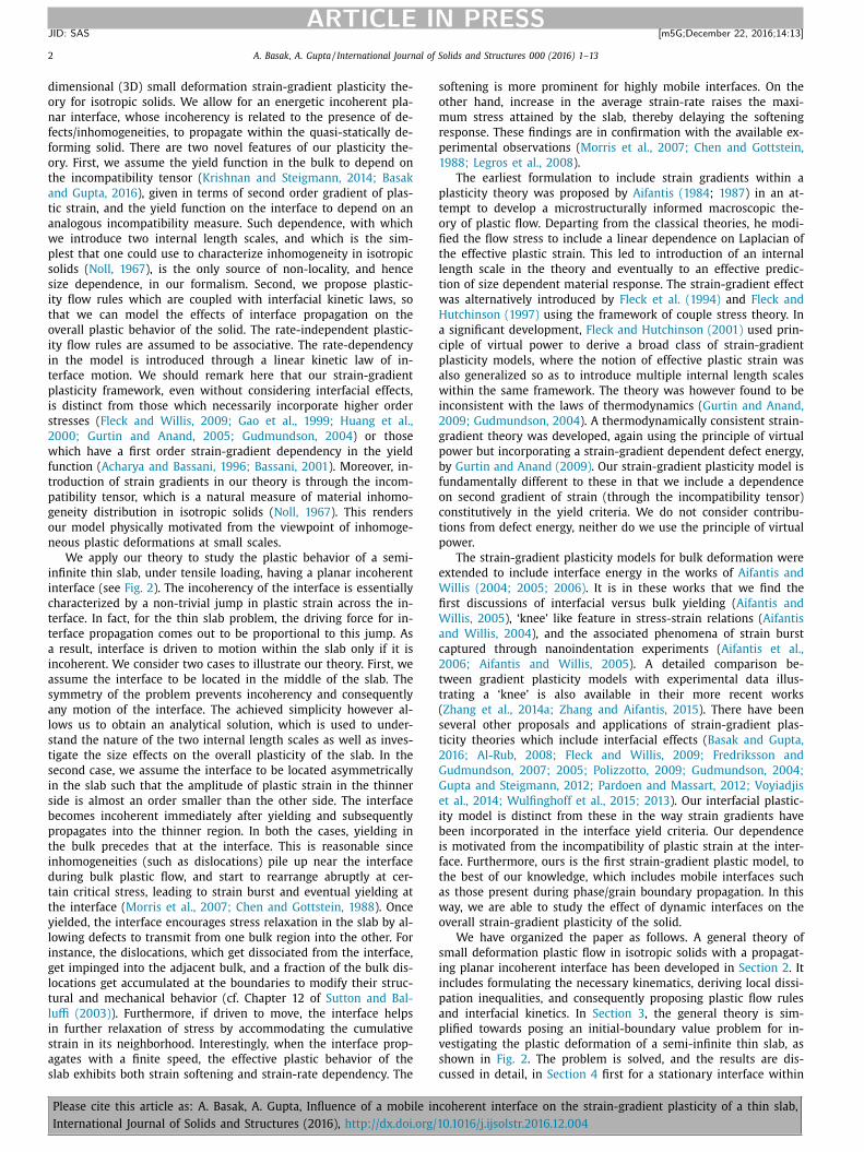
We apply our theory to study the plastic behavior of a semi-
infinite thin slab, under tensile loading, having a planar incoherent
interface (see Fig. 2 ). The incoherency of the interface is essentially
characterized by a non-trivial jump in plastic strain across the in-
terface. In fact, for the thin slab problem, the driving force for in-
terface propagation comes out to be proportional to this jump. As
a result, interface is driven to motion within the slab only if it is
incoherent. We consider two cases to illustrate our theory. First, we
assume the interface to be located in the middle of the slab. The
symmetry of the problem prevents incoherency and consequently
any motion of the interface. The achieved simplicity however al-
lows us to obtain an analytical solution, which is used to under-
stand the nature of the two internal length scales as well as inves-
tigate the size effects on the overall plasticity of the slab. In the
second case, we assume the interface to be located asymmetrically
in the slab such that the amplitude of plastic strain in the thinner
side is almost an order smaller than the other side. The interface
becomes incoherent immediately after yielding and subsequently
propagates into the thinner region. In both the cases, yielding in
the bulk precedes that at the interface. This is reasonable since
inhomogeneities (such as dislocations) pile up near the interface
during bulk plastic flow, and start to rearrange abruptly at cer-
tain critical stress, leading to strain burst and eventual yielding at
the interface ( Morris et al., 2007; Chen and Gottstein, 1988 ). Once
yielded, the interface encourages stress relaxation in the slab by al-
lowing defects to transmit from one bulk region into the other. For
instance, the dislocations, which get dissociated from the interface,
get impinged into the adjacent bulk, and a fraction of the bulk dis-
locations get accumulated at the boundaries to modify their struc-
tural and mechanical behavior (cf. Chapter 12 of Sutton and Bal-
luffi (2003) ). Furthermore, if driven to move, the interface helps
in further relaxation of stress by accommodating the cumulative
strain in its neighborhood. Interestingly, when the interface prop-
agates with a finite speed, the effective plastic behavior of the
slab exhibits both strain softening and strain-rate dependency. The
Please cite this article as: A . Basak, A . Gupta, Influence of a mobile in
International Journal of Solids and Structures (2016), http://dx.doi.org/1
oftening is more prominent for highly mobile interfaces. On the
ther hand, increase in the average strain-rate raises the maxi-
um stress attained by the slab, thereby delaying the softening
esponse. These findings are in confirmation with the available ex-
erimental observations ( Morris et al., 2007; Chen and Gottstein,
988; Legros et al., 2008 ).
The earliest formulation to include strain gradients within a
lasticity theory was proposed by Aifantis (1984 ; 1987 ) in an at-
empt to develop a microstructurally informed macroscopic the-
ry of plastic flow. Departing from the classical theories, he modi-
ed the flow stress to include a linear dependence on Laplacian of
he effective plastic strain. This led to introduction of an internal
ength scale in the theory and eventually to an effective predic-
ion of size dependent material response. The strain-gradient effect
as alternatively introduced by Fleck et al. (1994) and Fleck and
utchinson (1997) using the framework of couple stress theory. In
significant development, Fleck and Hutchinson (2001) used prin-
iple of virtual power to derive a broad class of strain-gradient
lasticity models, where the notion of effective plastic strain was
lso generalized so as to introduce multiple internal length scales
ithin the same framework. The theory was however found to be
nconsistent with the laws of thermodynamics ( Gurtin and Anand,
0 09; Gudmundson, 20 04 ). A thermodynamically consistent strain-
radient theory was developed, again using the principle of virtual
ower but incorporating a strain-gradient dependent defect energy,
y Gurtin and Anand (2009) . Our strain-gradient plasticity model is
undamentally different to these in that we include a dependence
n second gradient of strain (through the incompatibility tensor)
onstitutively in the yield criteria. We do not consider contribu-
ions from defect energy, neither do we use the principle of virtual
ower.
The strain-gradient plasticity models for bulk deformation were
xtended to include interface energy in the works of Aifantis and
illis (20 04; 20 05; 20 06) . It is in these works that we find the
rst discussions of interfacial versus bulk yielding ( Aifantis and
illis, 2005 ), ‘knee’ like feature in stress-strain relations ( Aifantis
nd Willis, 2004 ), and the associated phenomena of strain burst
aptured through nanoindentation experiments ( Aifantis et al.,
0 06; Aifantis and Willis, 20 05 ). A detailed comparison be-
ween gradient plasticity models with experimental data illus-
rating a ‘knee’ is also available in their more recent works
Zhang et al., 2014a; Zhang and Aifantis, 2015 ). There have been
everal other proposals and applications of strain-gradient plas-
icity theories which include interfacial effects ( Basak and Gupta,
016; Al-Rub, 2008; Fleck and Willis, 2009; Fredriksson and
udmundson, 20 07; 20 05; Polizzotto, 20 09; Gudmundson, 20 04;
upta and Steigmann, 2012; Pardoen and Massart, 2012; Voyiadjis
t al., 2014; Wulfinghoff et al., 2015; 2013 ). Our interfacial plastic-
ty model is distinct from these in the way strain gradients have
een incorporated in the interface yield criteria. Our dependence
s motivated from the incompatibility of plastic strain at the inter-
ace. Furthermore, ours is the first strain-gradient plastic model, to
he best of our knowledge, which includes mobile interfaces such
s those present during phase/grain boundary propagation. In this
ay, we are able to study the effect of dynamic interfaces on the
verall strain-gradient plasticity of the solid.
We have organized the paper as follows. A general theory of
mall deformation plastic flow in isotropic solids with a propagat-
ng planar incoherent interface has been developed in Section 2 . It
ncludes formulating the necessary kinematics, deriving local dissi-
ation inequalities, and consequently proposing plastic flow rules
nd interfacial kinetics. In Section 3 , the general theory is sim-
lified towards posing an initial-boundary value problem for in-
estigating the plastic deformation of a semi-infinite thin slab, as
hown in Fig. 2 . The problem is solved, and the results are dis-
ussed in detail, in Section 4 first for a stationary interface within
coherent interface on the strain-gradient plasticity of a thin slab,
0.1016/j.ijsolstr.2016.12.004
A. Basak, A. Gupta / International Journal of Solids and Structures 0 0 0 (2016) 1–13 3
ARTICLE IN PRESS
JID: SAS [m5G; December 22, 2016;14:13 ]
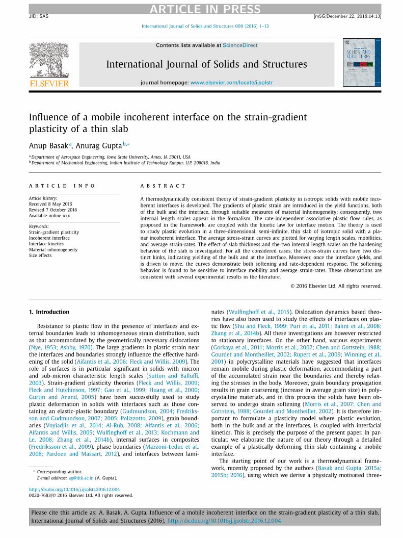
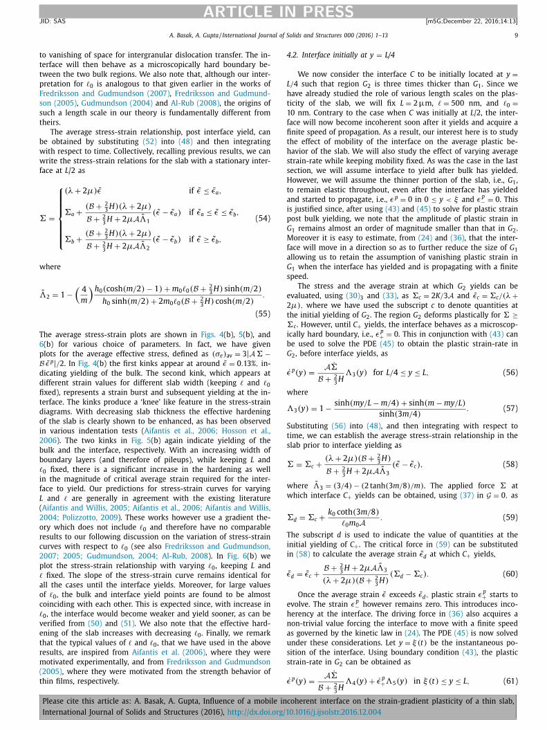
Fig. 1. A 3D region P ⊂ G with a planar interface � ⊂ C . Here, n is the fixed unit
normal to the interface and m is the outward unit normal to the boundary ∂P .
Fig. 2. A semi-infinite slab G with a planar incoherent interface C . The thickness of
the slab is L, �( t ) is the applied stress, and ξ ( t ) is the instantaneous position of the
interface at time t .
t
o
2
d
e
i
w
i
c
e
t
t
k
3
a
b
u
e
s
i
s
a
d
G
f
〈
a
i
e
�
w
p
t
v
m
r
t
∂
v
l
2
d
d
s
ω
a
β
T
t
t
ε
w
s
0
d
b
S
s
t
a
G
w
a
s
fi
t
t
a
s
E
w
s
he slab and then for a propagating interface. Finally, we conclude
ur work in Section 5 .
. General theory
In this section we introduce a 3D isothermal framework for
eveloping a thermodynamically consistent small deformation
lastic-plastic theory for single-phase isotropic solids with mobile
ncoherent interfaces. We restrict ourselves to planar interfaces
ith well defined normals. After introducing necessary kinemat-
cs we postulate a global dissipation inequality which, under spe-
ific constitutive assumptions on the nature of bulk and interface
nergy, yields local dissipation inequalities for the bulk and the in-
erfacial region. These local relations are then used to derive both
he plasticity flow rules (for bulk and interface) and the interfacial
inetic law.
The solid body under consideration occupies a subset G of the
D Euclidean point space. It contains a singular interface C with
constant unit normal n . Let P ⊂ G be an arbitrary region in the
ody such that � = P ∩ C is nonempty (see Fig. 1 ). The outward
nit normal to the boundary ∂P of P is denoted by m . The gradi-
nt of a differentiable bulk vector field f , with respect to the po-
Please cite this article as: A . Basak, A . Gupta, Influence of a mobile in
International Journal of Solids and Structures (2016), http://dx.doi.org/1
ition in G , is a tensor field denoted as ∇f , whereas its divergence
s given by div f . The material time derivative of f is indicated by a
uperposed dot. We have denoted time as t . The surface gradient
nd the surface divergence of a differentiable interfacial field g are
enoted by ∇
S g and div S g , respectively ( Cermelli and Gurtin, 1994;
upta and Steigmann, 2012 ). For a piecewise continuous bulk field
, the jump and average across C are defined as � f � = f + − f − and
f 〉 = ( f + + f −) / 2 , respectively, where f + is the limiting value of f
t the interface as we approach the interface from the bulk region
nto which the normal n points ( f − is defined likewise). It can be
asily verified that
f 1 f 2 � = � f 1 � 〈 f 2 〉 + 〈 f 1 〉 � f 2 � , (1)
here f 1 and f 2 are two piecewise continuous bulk fields.
Additional notation is fixed as follows. The Euclidean inner
roduct of two second order tensors A and B is written as A · B ;
he related norm is denoted as | A |. The trace, transpose, and in-
erse of A are denoted by tr A , A
T , and A
−1 , respectively. The sym-
etric and skew parts of A are represented by sym( A ) and skw( A ),
espectively. The derivative of a scalar-valued differentiable func-
ion of A , say f ( A ), denoted by ∂ A f , is defined by f ( A + B ) = f ( A ) + A f · B + o(| B | ) , where o (| B |)/| B | → 0 as | B | → 0. The derivatives of
ector and tensor-valued differentiable functions are defined simi-
arly. The second order identity tensor is given by I .
.1. Kinematics
Let u be a continuous displacement field defined over G . The
isplacement gradient tensor, β = ∇ u , is however allowed to be
iscontinuous across C . The infinitesimal strain tensor field and the
pin tensor field, well defined away from C , are ε = sym ( β) and
= skw ( β) , respectively. The following decomposition of β into
n elastic part βe and a plastic part βp is assumed ( Kröner, 1981 ):
= βe + β
p . (2)
he above considerations are justified if we assume β, βe , and βp
o be small (of the same order). Consequently, the total strain and
otal spin are also decomposed into elastic and plastic parts as
= εe + εp and ω = ω
e + ω
p , (3)
here the notation is self explanatory. It is immediate that εe =ym ( β
e ) , εp = sym ( β
p ) , ω
e = skw ( βe ) , and ω
p = skw ( βp ) .
The continuity of u requires � u � = 0 , which implies � β� P = , where P = I − n � n is the projection tensor ( � denotes the
yadic product). The interfacial distortion tensor field can then
e unambiguously defined as G = β+ P = β−P = 〈 β〉 P ( Gupta and
teigmann, 2012 ). The interfacial strain field, defined as E =ym ( G ) , is related to the bulk strain field as E = P 〈 ε〉 P . Analogous
o the decomposition (2) in the bulk, the interfacial distortion is
dditively decomposed into elastic and plastic parts as
= G
e γ + G
p γ = G
e δ + G
p
δ, (4)
here G
e γ = β
e + P , G
e δ = β
e −P , G
p γ = β
p + P , and G
p
δ= β
p −P ; see Gupta
nd Steigmann (2012) and Basak and Gupta (2016) for the corre-
ponding multiplicative decomposition when the deformations are
nite. Here, the subscripts δ and γ have been used to differentiate
he two disjoint surfaces obtained from the incoherent interface in
he intermediate configuration ( Gupta and Steigmann, 2012; Basak
nd Gupta, 2016 ). The decomposition of the interfacial strain ten-
or follows subsequently as
= E
e γ + E
p γ = E
e δ + E
p
δ, (5)
here E
e γ = P εe + P , E
e δ = P εe −P , E
p γ = P εp
+ P , and E
p
δ= P εp
−P are re-
pective interfacial elastic and plastic strain fields. The incoherency
coherent interface on the strain-gradient plasticity of a thin slab,
0.1016/j.ijsolstr.2016.12.004
4 A. Basak, A. Gupta / International Journal of Solids and Structures 0 0 0 (2016) 1–13
ARTICLE IN PRESS
JID: SAS [m5G; December 22, 2016;14:13 ]
V
a
t
g
l
i
σ
V
w
i
2
i
t
t
a
f
w
a
M
t
σ
B
F
(
V
2
t
i
t
s
s
g
s
2
w
s
s
B
i
o
i
t
v
(
t
a
F
tensor, which measures the relative elastic (or plastic) distortion
between γ and δ sides of the interface, is given by
M = G
e δ − G
e γ = G
p γ − G
p
δ, (6)
cf. Gupta and Steigmann (2012) and Cermelli and Gurtin (1994) for
definition of the incoherency tensor in the finite deformation
framework. For a coherent interface, G
e δ = G
e γ and G
p γ = G
p
δ, the in-
coherency tensor vanishes identically.
Let g be a smooth field defined over the interface C . The nor-
mal time derivative of g following C is given by Gurtin and Jabbour
(2002)
g =
˙ g + V ∇g · n , (7)
where V is the normal velocity field of the interface. It quantifies
the rate of change of g as observed by an observer sitting on the
moving interface. The parametrization independent intrinsic veloc-
ity of the edge ∂� of � is given by Gurtin and Jabbour (2002)
q = V n + W t , (8)
where W is the component of the edge velocity along a direction
(quantified with unit vector t ) which is both tangential to the in-
terface and normal to the curve ∂�.
2.2. Dissipation inequality
Recall region P as introduced in the beginning of Section 2 and
shown in Fig. 1 . Assuming that P does not exchange mass with its
surrounding, and neglecting excess mass density at the interface,
we have the following local mass balance laws: ˙ ρ = 0 in G \ C and
� ρ� = 0 over C , where ρ is the mass density of the bulk ( Gupta
and Steigmann, 2012 ). These imply that density is time indepen-
dent and continuous across the singular interface, allowing the in-
terface to be mobile. The linear momentum balance for the re-
gion P , while neglecting interfacial stresses, body forces, and in-
ertia, yields ( Gupta and Steigmann, 2012 )
div σ = 0 in G \ C and � σ� n = 0 over C, (9)
where σ is the symmetric bulk Cauchy stress tensor.
According to a mechanical version of the second law of thermo-
dynamics, the rate of change of the total free energy of P is always
less than or equal to the net power input into P . Neglecting kinetic
energies of the bulk and interface, we postulate the dissipation in-
equality as ( Basak and Gupta, 2015a; 2015b; 2016 )
d
dt
(∫ P
dv +
∫ �
da
)≤
∫ ∂P
σm · v da +
∫ ∂�
c · q dl. (10)
Here is the free energy in the bulk per unit volume, is the
free energy of the interface per unit area, v is the material velocity
field, dv is an infinitesimal volume element, da is an infinitesimal
area element, and dl is an infinitesimal length element. The first
term on the right hand side of the inequality denotes the mechan-
ical power input to P through the working of traction on the outer
surface ∂P . The second term is a non-standard power input to P
considered to ensure that the entropy production is restricted only
to within the bulk and interface, i.e., there is no entropy generation
at the arbitrary edge of the interface ∂� ( Basak and Gupta, 2015a;
2015b; 2016 ). The exact form of c will depend on the constitutive
form of the energies. Using the standard transport relations and
divergence theorems, inequality (10) can be rewritten as ∫ P
(div ( σv ) − ˙
)dv +
∫ �
(V � � + � σv � · n −
)da
+
∫ ∂�
( c · q − W ) dl ≥ 0 . (11)
The last term on the left hand side of the inequality should vanish
identically, since otherwise it will represent an unphysical contri-
bution to the entropy. Considering energies of the form =
ˆ ( εe )
Please cite this article as: A . Basak, A . Gupta, Influence of a mobile in
International Journal of Solids and Structures (2016), http://dx.doi.org/1
nd =
ˆ ( M ) , we thereby require c · n = 0 and c · t = . Addi-
ionally, we assume plastic incompressiblity (i.e., tr εp = 0 ). The
lobal dissipation inequality (11) can then be shown to be equiva-
ent to the constitutive relation σ = ∂ εe ˆ and the local dissipation
nequalities
d · ˙ εp ≥ 0 in G \ C and (12)
f n − B · M ≥ 0 over C, (13)
here σd = σ − ( tr σ) I / 3 is the deviatoric part of σ , B = ∂ M
ˆ , and
f n = � I − βT σ� n · n (14)
s the driving force for interface propagation ( Basak and Gupta,
016; Gupta and Steigmann, 2012 ). According to (12) , dissipation
n the bulk is only due to plastic evolution, whereas dissipation at
he interface is an outcome of both the kinetics of interfacial mo-
ion as well as the evolution of the incoherency tensor.
To be more specific, we use quadratic energy densities which,
fter considerations of isotropic material symmetry, have a general
orm
ˆ ( εe ) =
λ
2
( tr εe ) 2 + μ εe · εe and (15)
ˆ ( M ) = 0 +
b 0 2
( tr M s ) 2 + b 1 (| M s | 2 + | M a | 2 ) , (16)
here λ and μ are the Lamé constants in the bulk, b 0 and b 1 re the moduli of incoherency for the interface, M s = sym ( M ) ,
a = skw ( M ) , and 0 is the constant interfacial tension. From
hese expressions we can obtain
= λ( tr εe ) I + 2 μεe and (17)
= b 0 ( tr M s ) P + 2 b 1 ( M s + M a ) . (18)
inally, if M a = 0 then, noting that M s = E
p γ − E
p
δ, we can rewrite
13) as
f n − B · E
p
γ + B · E
p
δ ≥ 0 over C. (19)
.3. Plastic flow rules and interfacial kinetics
Based on dissipation inequalities (12) and (19) we now derive
he plastic flow rules, both in the bulk and at the interface, and
nterfacial kinetic equations. The plastic evolution will be assumed
o be rate-independent and associative. We will depart from clas-
ical plasticity by assuming the yield functions to depend on mea-
ures of material inhomogeneity, represented in terms of suitable
radients of plastic strain. Such dependence is the only source of
train-gradient effects in our theory.
.3.1. Bulk plasticity
In order to incorporate non-locality in our plasticity model,
e assume the yield function to depend on a suitable mea-
ure of material inhomogeneity, besides its usual dependence on
tress and effective plastic strain. It is well established ( Noll, 1967;
asak and Gupta, 2016; Krishnan and Steigmann, 2014 ) that, under
sotropic material symmetry, material inhomogeneity is unambigu-
usly represented by the material curvature tensor (whose vanish-
ng provides necessary conditions for strain compatibility). When
he strains are small, as is presently the case, the material cur-
ature reduces to Kröner’s incompatibility tensor η = curl curl εp
Kröner, 1981 ). With this in mind, we consider the yield locus in
he deviatoric stress space (parametrized by effective plastic strain
nd incompatibility tensor) to be given by F = 0 , where
=
˜ F ( σd , E p , η) . (20)
coherent interface on the strain-gradient plasticity of a thin slab,
0.1016/j.ijsolstr.2016.12.004
A. Basak, A. Gupta / International Journal of Solids and Structures 0 0 0 (2016) 1–13 5
ARTICLE IN PRESS
JID: SAS [m5G; December 22, 2016;14:13 ]
I
w
s
i
t
t
F
w
i
ε
w
β
(
c
r
t
a
2
w
V
w
i
h
w
i
d
f
d
k
V
w
(
y
B
e
y
G
H
2
r
t
a
i
s∮
w
−κ
w
s
s
i
o
p
B
t
o
c
i
(
t
G
w
p
i
E
w
t
r
i
t
3
a
F
T
z
t
a
i
m
c
t
s
t
a
fi
m
t
c
t
s
d
t
l
a
t
b
ε
o
σ
O
σ
e
σ
w
A
n the above equation, E p =
∫ t 0
˙ E p dτ is the effective plastic strain
ith
˙ E p =
√ (2 εp · ˙ εp
)/ 3 . Under the assumption of isotropic re-
ponse, ˜ F can depend on σd and η only through their principal
nvariants. We will in fact consider yield functions which are func-
ions of only the second invariant of σd (the first invariant of σd is
rivially zero) and the first invariant of η (denoted by η), i.e.,
=
ˆ F (σe , E p , η) , (21)
here σe =
√ (3 σd · σd
)/ 2 . The principle of maximum dissipation,
n conjunction with (12) , yields the associative flow rule
˙ p =
˙ β ∂ σd ˆ F , (22)
here ˙ β ≥ 0 is the plastic multiplier. The consistency condition
˙ ˙ ˆ F = 0 will result into a second order partial differential equation
PDE) for the plastic strain-rates whenever ˙ β > 0 . The boundary
onditions required for solving the PDE are provided by the flow
ules at the interface and the microscopic conditions on the plas-
ic strain-rate and/or their spatial derivative at the external bound-
ries of the solid, as discussed next.
.3.2. Interfacial kinetics and interfacial flow rules
To derive the plastic flow rules and the kinetic relation we start
ith conditions
f n ≥ 0 and B γ · E
p
γ + B δ · E
p
δ ≥ 0 over C, (23)
hich are sufficient for dissipation inequality (19) . Here we have
ntroduced B γ = −B and B δ = B . The interface C is assumed to be
omophase, requiring dissipation inequality (23) 2 to be symmetric
ith respect to suffixes γ and δ. This is indeed true as can be ver-
fied using (18) in the inequality. Although we have decoupled the
issipation inequalities pertaining to interface kinetics and inter-
ace plasticity, the two phenomena remain coupled to each other
ue to the nature of normal time derivatives.
Motivated by dissipation inequality (23) 1 we postulate a linear
inetic relation of the form
= M f n , (24)
here M ≥ 0 is the constant interface mobility and f n is given by
14) .
Analogous to our considerations in the bulk, we assume the
ield function at the interface to depend on generalized stresses
γ and B δ , parameterized by the effective interfacial plastic strain
p , and an appropriate measure of material inhomogeneity κ. The
ield locus is given by G = 0 , where
=
˜ G ( B γ , B δ, e p , κ) . (25)
ere e p =
∫ t 0 e
p dτ with e p =
√
| E
p
γ | 2 + | E
p
δ | 2 ( Basak and Gupta,
016 ). For κ, under small strain assumption, we look for a rep-
esentation of the incompatibility tensor on the interface. Toward
his end, we consider a closed curve C 1 in P such that it encloses
n area A 1 and intersects � at two points. Let C 2 be the line of
ntersection of A 1 with �. The Stokes’ theorem for a piecewise
mooth field curl εp then yields ( Gupta and Steigmann, 2012 )
C 1
curl εp d x =
∫ A 1
( curl curl εp ) T N da −∫
C 2
� curl εp � d x , (26)
here N is the unit normal to A 1 . Define κ such that � curl εp � d x =κT t 1 dl, where t 1 is the unit tangent along C 2 . Hence
T = � curl εp � ( t 1 � t 2 − t 2 � t 1 ) , (27)
here t 2 is a unit vector on the tangential plane of the interface
uch that { t 1 , t 2 , n } form a positively oriented orthonormal ba-
is. It is immediately clear that vanishing of incompatibility tensor,
.e., curl curl εp = 0 , is not sufficient to ensure path independence
Please cite this article as: A . Basak, A . Gupta, Influence of a mobile in
International Journal of Solids and Structures (2016), http://dx.doi.org/1
f the closed integral in (26) , which is otherwise required for im-
osing continuity of the displacement field (cf. pages 84–100 from
oley and Weiner, 1997 ). The additional condition is provided by
he last integral in (26) , which essentially requires vanishing of κver the interface; hence κ can be regarded as an interfacial in-
ompatibility measure. It can be easily checked that κ, as defined
n (27) , is independent of the choice of basis vectors t 1 and t 2 Gupta and Steigmann, 2012 ).
For our purposes in the following sections, we restrict ourselves
o yield functions of the form
=
ˆ G (τe , e p , κ) , (28)
here τe =
√ | B γ | 2 + | B δ| 2 is the effective stress, and κ is the first
rincipal invariant of κ. The postulation of maximum dissipation,
n conjunction with (23) , yields the associative flow rules
˚
p
γ = ζ ∂ B γ ˆ G and E
p
δ = ζ ∂ B δ ˆ G , (29)
here ζ ≥ 0 is the plastic multiplier for the interface. The consis-
ency condition ζ ˚ G = 0 , combined with flow rules (29) and kinetic
elation (24) , can be solved to evaluate plastic strain-rates at the
nterface. These serve as the boundary conditions for the PDE ob-
ained from the consistency condition in the bulk.
. Slab with a propagating interface
The body G is now taken to be a semi-infinite thin slab with
moving planar interface C having fixed orientation n = e 2 , see
ig. 2 . The interface divides the slab into two parts G 1 and G 2 .
he components of the position vector x are denoted by x, y , and
with respect to Cartesian basis vectors e 1 , e 2 , and e 3 , respec-
ively. The slab is subjected to uniform uniaxial tensile force �( t )
t the free boundary. The instantaneous position of the interface
s denoted by y = ξ (t) . In the following we simplify the plasticity
odel, proposed in Section 2.3 , under additional kinematical and
onstitutive assumptions and collect the governing equations for
he initial-boundary value plasticity problem. The solution to the
emi-infinite thin slab problem, as discussed in the following sec-
ions, can be related to several problems of practical interest, such
s a bicrystal subjected to external loading ( Al-Rub, 2008 ) or a thin
lm on a substrate under external loading ( Fredriksson and Gud-
undson, 2007; 2005 ).
We consider a displacement field such that only ε22 is non-
rivial while all other components of the total strain remain identi-
ally zero. We assume all the fields, including strains and stresses,
o be independent of coordinates x and z . We also assume the
hear components of elastic and plastic strains to be zero. Ad-
itionally, elastic and plastic spin tensor fields are both assumed
o vanish, yielding M a = 0 . Moreover, the symmetry of the prob-
em allows us to assume εe 11
= εe 33
and εp 11
= εp 33
. We denote ε22
nd εp 22
as ε and εp , respectively. The plastic incompressibility can
hen be used to obtain εp 11
= εp 33
= −εp / 2 . This result, when com-
ined with strain decomposition (3) 1 , yields εe 11
= εe 33
= εp / 2 ande 22
= ε − εp . The non-trivial components of the bulk stress can be
btained from (17) as
11 = σ33 = λε + με p and σ22 = (λ + 2 μ) ε − 2 με p . (30)
n the other hand, equilibrium Eq. (9) 1 can be used to write
22 = �(t) . The components of the deviatoric stresses can then be
xpressed as
d 11 = σ d
33 = −σ d 22 / 2 and σ d
22 = A � − B ε p , (31)
here
=
4 μ
3(λ + 2 μ) and B =
2 μ(3 λ + 2 μ)
3(λ + 2 μ) . (32)
coherent interface on the strain-gradient plasticity of a thin slab,
0.1016/j.ijsolstr.2016.12.004
6 A. Basak, A. Gupta / International Journal of Solids and Structures 0 0 0 (2016) 1–13
ARTICLE IN PRESS
JID: SAS [m5G; December 22, 2016;14:13 ]
c
t
i
w
|
T
i
m
i
s
t
ε
F
t
ε
T
i
d
a
4
s
s
t
s
s
h
t
p
p
s
E
2
e
t
μ
a
4
M
e
c
p
�
f
F
i
t
l
t
o
To obtain equations of bulk plasticity, we begin by noting the
simplified expressions for effective stress σe = 3 | σ d 22
| / 2 = 3 |A � −B εp | / 2 , equivalent plastic strain-rate ˙ E p = | εp | , and first invariant
of incompatibility tensor η = −∂ 2 εp / ∂y 2 . Moreover, we assume the
yield function (21) to be a linear function of all its arguments, i.e.,
F = σe − ( K + HE p + c η) , (33)
where K is the constant flow stress, H is the plastic modulus, and
c is a phenomenological constant with a unit of force. This form
reduces to a yield function in classical plasticity theory if the co-
efficient c , associated with the non-local term, vanishes identically.
The flow rule (22) now reduces to
˙ ε p =
˙ β sign (A � − Bε p ) , (34)
where sign( x ) is equal to −1 if x < 0, 0 if x = 0 , and 1 if x > 0.
When
˙ E p > 0 , the consistency condition
˙ E p ˙ F = 0 yields
3
2
sign (A � − B ε p )(A
˙ � − B ε p ) − H| ε p | + c ∂ 2 ˙ ε p
∂y 2 = 0 , (35)
which is a PDE for ˙ εp . This is to be supplemented with the bound-
ary conditions at the interface and the external boundaries y = 0 , L,
as derived in the following.
The kinetics of the interface is governed by (24) where the driv-
ing force f n , given by (14) , is now of the form
f n =
μ(3 λ + 2 μ)
2(λ + 2 μ) � ( ε p ) 2 � − 2 μ�
λ + 2 μ� ε p � . (36)
To derive plasticity equations at the interface we begin by assum-
ing the yield function (28) to be linear in terms of its arguments,
i.e.,
G = τe − ( k 0 + h 0 e p + c 0 κ) , (37)
where k 0 is the yield strength, h 0 is the plastic modulus, and c 0 is a material constant whose physical interpretation would be dis-
cussed later. Note that k 0 is similar to interfacial tension 0 in that
it resists the plastic flow near the interface ( Aifantis et al., 2006 ).
Furthermore, with E
e γ = ( εp
+ / 2) P , E
e δ = ( εp
−/ 2) P , E
p γ = −( εp
+ / 2) P ,
E
p
δ= −( εp
−/ 2) P , and M = −(( εp
+ − εp −) / 2
)P , we can write B =
−(b 0 + b 1 )(εp + − εp
−) P and consequently obtain
τe = 2 | (b 0 + b 1 )(εp + − ε p
−) | (38)
and
e p =
1 √
2
√
( ε p + ) 2 + ( ε p
−) 2 . (39)
Also, κ = −� ∂ εp / ∂y � (considering t 1 = e 3 and t 2 = e 1 in (27) ).
When B is non-vanishing, i.e., εp + � = εp
−, flow rules (29) are reduced
to
ε p + = ζ T and ε p
− = −ζ T , (40)
where T = −sign ((b 0 + b 1 )(εp + − εp
−)) . On substituting these into
(39) we get ζ = e p , and from consistency condition ζ G = 0 (for
ζ > 0 ) we obtain
ζ =
c 0 h eff
�
˚∂ ε p / ∂y
�
, (41)
where h eff = h 0 + 4(b 0 + b 1 ) is an effective measure of plastic
modulus of the interface. These relations, upon using the definition
of normal time derivative, can be used to solve for plastic strain-
rates at the interface, which provides us with boundary conditions
at the interface y = ξ required for solving (35) .
In the above framework nontrivial kinetic and flow relations are
obtained only when the interface is incoherent, i.e., when εp + � = εp
−.
This can be seen by identical vanishing of both the driving force
(and hence V ) and strain-rates in (36) and (40) . If the interface is
Please cite this article as: A . Basak, A . Gupta, Influence of a mobile in
International Journal of Solids and Structures (2016), http://dx.doi.org/1
oherent then we would still like to obtain an expression for plas-
ic strain-rate at an otherwise stationary interface. We do so by us-
ng the consistency condition
˙ G = 0 (when | εp + | = | εp
−| > 0 ) which,
ith the help of (37) and (39) , reduces to
ε p + | = | ε p
−| =
c 0 h 0
� ∂ ˙ ε p / ∂y � . (42)
he above relations provide boundary conditions at y = ξ for solv-
ng (35) when the plastic strain is continuous at the interface.
The interfacial conditions derived above should be supple-
ented with boundary conditions at the external surface. Follow-
ng standard practice ( Anand et al., 2005 ), we assume the external
urfaces at y = 0 , L to be non-dissipative and properly coated so
hat they behave as microscopically hard boundaries, i.e.,
˙ p = 0 at y = 0 , L. (43)
urthermore, we assume that there is no residual plastic strain (at
he initial time) in the bulk, interface, and external boundaries,
p (y, 0) = 0 for 0 ≤ y ≤ L. (44)
o summarize, the complete initial-boundary value problem for εp
ncludes simultaneously solving (34) and (35) with the initial con-
ition (44) and the boundary conditions (43) . To these we should
dd conditions (40) - (41) , when εp + � = εp
−, or (42) , when εp + = εp
−.
. Results and discussion
The initial-boundary value problem, formulated in the previous
ection, is now solved to study the effect of an interface on the
train-gradient plasticity of a semi-infinite micro-slab. We consider
wo cases with initial position of the interface at L /2 and L /4, re-
pectively. In the former, due to symmetry, the interface remains
tationary during the deformation of the slab. In the latter case,
owever, the interface propagates with a finite speed so as to fur-
her reduce the thickness of the thinner region. In all our exam-
les, in order to highlight the role of the interface on the overall
lasticity of the slab, we calculate both the distribution of plastic
train field and the average stress-strain behavior in the slab.
For all our calculations we assume modulus of elasticity of bulk
= 100 GPa, Poisson’s ratio of bulk ν = 0 . 3 , K = 100 MPa, H =0 GPa, k 0 = 0 . 08 N/m, h 0 = 10 N/m, b 0 + b 1 = −1 N/m ( Aifantis
t al., 2006; Al-Rub, 2008 ). The Lamé constants λ and μ are ob-
ained using the standard relations λ = Eν/ ((1 − 2 ν)(1 + ν)
)and
= E/ (2(1 + ν)) . We define the average of a bulk field, say f ( y ),
s f = (1 /L ) ∫ L
0 f (y ) dy .
.1. Interface at y = L/2
We assume the mean total strain ε to remain non-negative.
oreover, in accordance with experimental observations ( Aifantis
t al., 2006 ), we will assume interface yielding to be always pre-
eded by yielding in the bulk. Before the bulk starts to deform
lastically, there exists a constant strain field in G given by ε =/ (λ + 2 μ) , as calculated from (30) 3 with εp = 0 . The applied
orce �, at which yielding initiates, can be obtained by putting
= 0 in (33) as �a = 2 K / 3 A . The subscript a has been used to
ndicate the value of the variable at initial yielding of the bulk. In
erms of strain, εa = εa = �a / (λ + 2 μ) . When � > �a , or equiva-
ently ε > εa , the plastic strain field evolves in the bulk (away from
he interface). Assuming ˙ εp > 0 , the PDE governing the evolution
f plastic strain can then be obtained from (34) and (35) as
∂ 2 ˙ ε p
∂y 2 − 1
� 2 ˙ ε p = − A
˙ �
� 2 (B +
2 3
H) , (45)
coherent interface on the strain-gradient plasticity of a thin slab,
0.1016/j.ijsolstr.2016.12.004
A. Basak, A. Gupta / International Journal of Solids and Structures 0 0 0 (2016) 1–13 7
ARTICLE IN PRESS
JID: SAS [m5G; December 22, 2016;14:13 ]
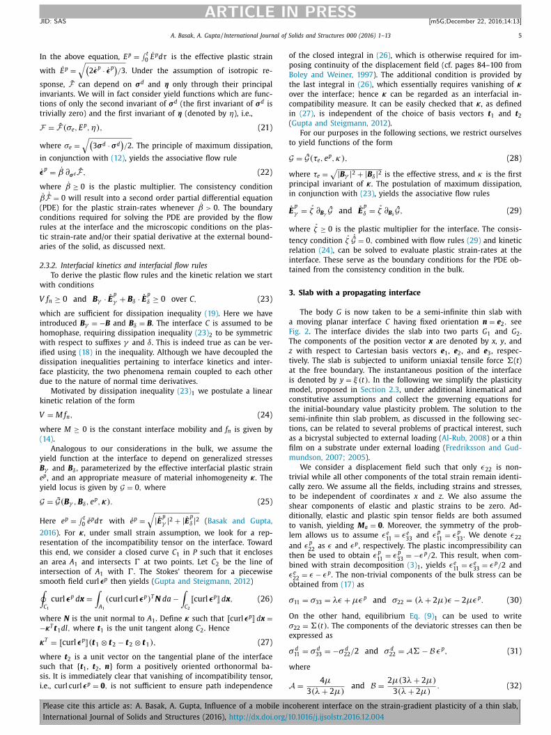
Fig. 3. Non-dimensional plastic strain-rate �1 , before interface has yielded, for var-
ious m when the interface is located at y = L/ 2 .
w
w
c
t
s
t
p
A
t
d
(
i
t
t
b
2
ε
i
ε
w
�
�
i
n
t
t
t
(
T
p
d
e
l
a
ε
t
i
�
w
r
T
d
s
(
�
w
a
i
�
t
p
s
t
t
a
t
�
ε
b
t
(
l
a
i
r
p
i
i
w
(
ε
w
y/L )]
2 m 0 �
L − m
+ 2 m
here � 2 = c/ ( 3 B/ 2 + H ) is an internal length scale associated
ith the inhomogeneity within the bulk (we assume c > 0). It is
lear that incorporating a non-trivial � in the theory is tantamount
o bringing second-order effects in the plastic evolution. The length
cale � can also be seen as controlling the effective hardening of
he solid due to inhomogeneous plastic deformation. It was inter-
reted as the length of dislocation pileup near the boundaries by
ifantis et al. (2006) . As � → 0, (45) leads to the classical plas-
icity solution of constant plastic strain in the entire slab. We will
iscuss more about � in our subsequent discussion. Equations like
45) were first proposed by Aifantis (1984) ; 1987 ) in an attempt to
ntroduce non-locality in plasticity theory. It should be emphasized
hat the appearance of the second-gradient term here is due to in-
roduction of incompatibility in the yield function, as compared to
eing derived from a micro force balance ( Gurtin and Anand, 2005;
009 ). Eq. (45) can be solved, using boundary conditions (43) and
˙ p + = ˙ εp
− = 0 (at y = L/ 2 ), to obtain plastic strain-rate field prior to
nterface yielding as
˙ p (y ) =
A
˙ �
B +
2 3
H
�1 (y ) , (46)
here
1 (y ) =
⎧ ⎪ ⎨
⎪ ⎩
1 − sinh (my/L ) + sinh (m/ 2 − my/L )
sinh (m/ 2) if 0 ≤ y ≤ L/ 2 ,
1 − sinh (my/L − m/ 2) + sinh (m − my/L )
sinh (m/ 2) if L/ 2 ≤ y ≤ L,
(47)
is the non-dimensional plastic strain-rate and m = L/� . Fig. 3 plots
1 for various m . For fixed L and increasing m , and hence decreas-
ng � , there are thinner boundary layers as well as increasing mag-
itudes of non-dimensional plastic strain-rates (bounded by 1). As
he internal length scale � approaches the thickness of the slab L ,
he amplitude of plastic strain-rate decreases making it difficult for
he slab to deform plastically. In such a case the inhomogeneities
such as dislocation pileups) occupy a larger fraction of the slab.
�2 (y ) =
⎧ ⎪ ⎪ ⎪ ⎪ ⎪ ⎨
⎪ ⎪ ⎪ ⎪ ⎪ ⎩
1 − h 0 [ sinh (my/L ) + sinh (m/ 2 − m
h 0 sinh (m/ 2) +
if 0 ≤ y ≤ L/ 2 and
1 − h 0 [ sinh (m − my/L ) + sinh (my/
h 0 sinh (m/ 2) if L/ 2 ≤ y ≤ L
Please cite this article as: A . Basak, A . Gupta, Influence of a mobile in
International Journal of Solids and Structures (2016), http://dx.doi.org/1
hese conclusions are qualitatively in agreement with recently re-
orted results of gradient plasticity predictions and 3D discrete
islocation dynamics simulations ( Zhang and Aifantis, 2015; Zhang
t al., 2014b ). We can now establish an average stress-strain re-
ation, prior to interface yielding, by first calculating the rate of
verage total strain using (30) 3 ,
˙ ¯ =
˙ �
λ + 2 μ+
2 μ
L (λ + 2 μ)
∫ L
0
˙ ε p dy, (48)
hen substituting plastic strain-rate from (46) into (48) , and finally
ntegrating the resulting expression with respect to time, as
= �a +
(B +
2 3
H)(λ + 2 μ)
B +
2 3
H + 2 μA �1
( ε − εa ) , (49)
here �1 = 1 − 4 tanh (m/ 4) /m .
At the onset of interface yielding, since εp + and εp
− remain zero,
elations (36) –(39) imply that both τ e and e p vanish identically.
he interface of course remains stationary due to vanishing of the
riving force. In order to calculate � at which interface yields, we
ubstitute (37) in G = 0 , and evaluate plastic strains by integrating
46) with respect to time, to obtain
b = �a +
k 0 2 � 0 m 0 A tanh (m/ 4)
, (50)
here we have introduced a new length scale � 2 0
= c 0 / (B +
2 3 H)
nd a non-dimensional parameter m 0 = � 0 /� . We use subscript b to
ndicate the value of the variable at the onset of interfacial yield.
0 characterizes the thickness of a region in the neighborhood of
he interface where the interactions between bulk and interfacial
lasticity remain concentrated. In particular, a smaller � 0 will re-
trict the interfacial plastic flow to a narrower region in addition
o increasing the value of �b , for fixed � . The parameter m 0 , on
he other hand, represents the fraction of boundary layer thickness
t the interface as a result of interfacial yielding. We can obtain
he average total strain at the onset of interface yielding, by using
= �b in (49) , as
¯b = εa +
B +
2 3
H + 2 μA �1
(λ + 2 μ)(B +
2 3
H) (�b − �a ) . (51)
So far we have investigated the plastic response of the slab
efore interface C has yielded. When � is increased beyond �b
here is a sudden transmission of plastic flow across the interface
Aifantis et al., 2006; Hosson et al., 2006; Morris et al., 2007 ). Fol-
owed by such strain burst, the plastic strains at the interface εp +
nd εp − evolve. Since the interface is located at L /2, the symmetries
n both geometry of the slab and external loading ensure that the
esponse remains symmetric about the interface and, in particular,
lastic strain field εp remains continuous across the interface. The
nterface therefore remains coherent at all times. The driving force
n (36) also vanishes keeping the interface stationary. As a result
e now solve (45) , with boundary conditions provided by (42) and
43) , to obtain
˙ p (y ) =
A
˙ �
B +
2 3
H
�2 (y ) , (52)
here
+ 2 m 0 � 0 (B +
2 3
H) cosh (m/ 2 − my/L )
0 (B +
2 3
H) cosh (m/ 2)
/ 2)] + 2 m 0 � 0 (B +
2 3
H) cosh (my/L − m/ 2)
0 � 0 (B +
2 3
H) cosh (m/ 2)
(53)
coherent interface on the strain-gradient plasticity of a thin slab,
0.1016/j.ijsolstr.2016.12.004
8 A. Basak, A. Gupta / International Journal of Solids and Structures 0 0 0 (2016) 1–13
ARTICLE IN PRESS
JID: SAS [m5G; December 22, 2016;14:13 ]
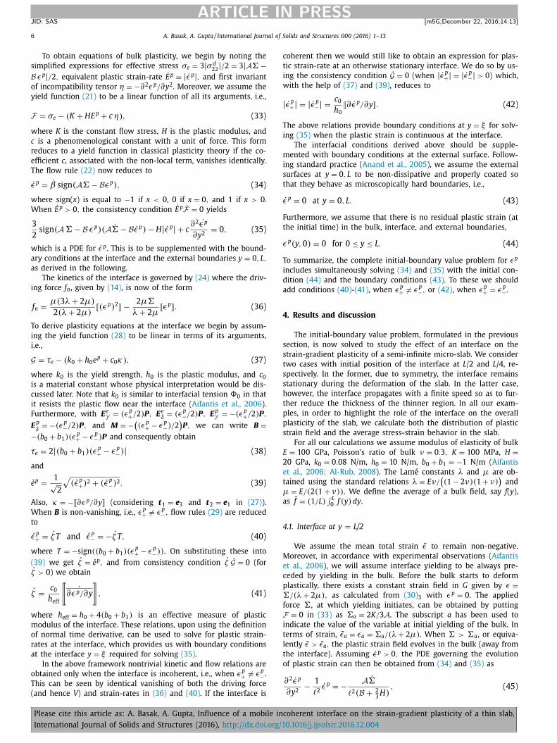
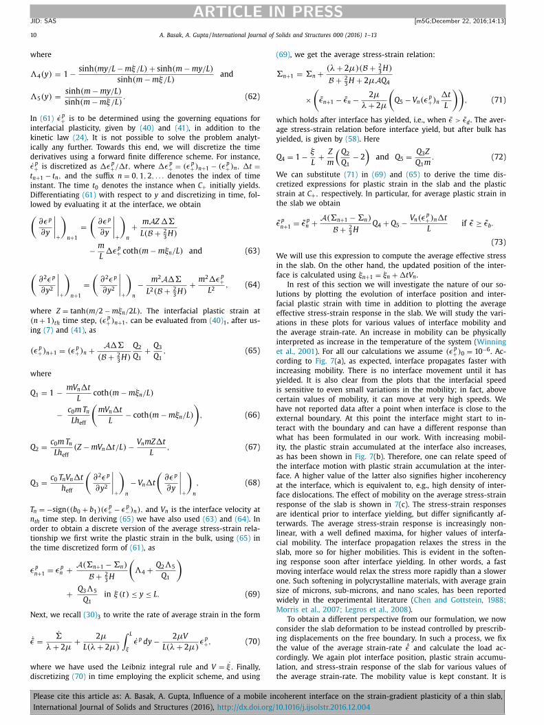
Fig. 4. (a) Non-dimensional plastic strain-rate �2 , post interface yield, and (b) the average effective stress-strain response for various L . We take � = 500 nm and � 0 = 10 nm.
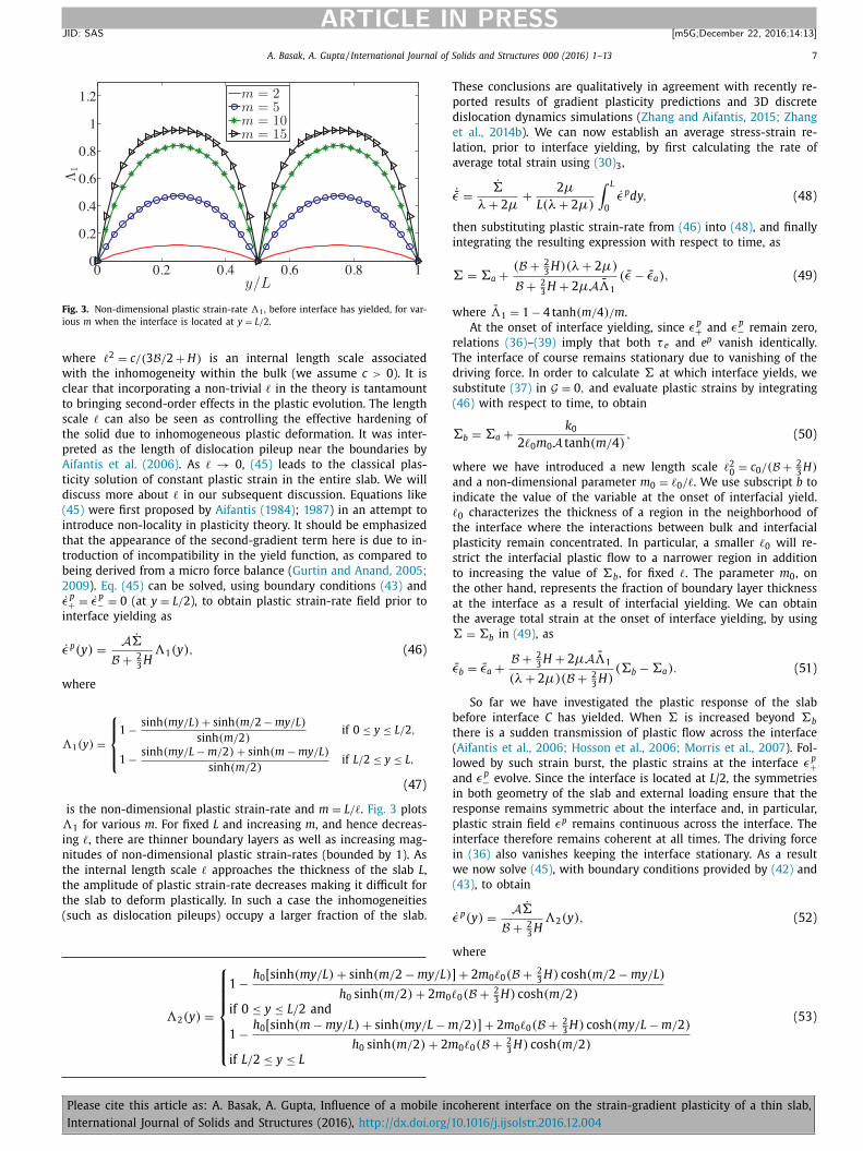
Fig. 5. (a) Non-dimensional plastic strain-rate �2 , post interface yield, and (b) the average effective stress-strain response for various � . We take L = 2 μm and � 0 = 10 nm.
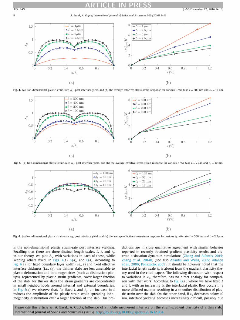
Fig. 6. (a) Non-dimensional plastic strain-rate �2 , post interface yield, and (b) the average effective stress-strain response for various � 0 . We take � = 500 nm and L = 2 . 5 μm .
d
r
c
Z
e
i
o
t
s
a
m
t
n
is the non-dimensional plastic strain-rate post interface yielding.
Recalling that there are three distinct length scales, L , � , and � 0 in our theory, we plot �2 with variations in each of these, while
keeping others fixed, in Figs. 4 (a), 5 (a), and 6 (a). According to
Fig. 4 (a), for fixed boundary layer width (i.e., � ) and fixed effective
interface thickness (i.e., � 0 ), the thinner slabs are less amenable to
plastic deformation and inhomogeneities (such as dislocation pile-
ups), represented by plastic strain gradients, cover larger fraction
of the slab. For thicker slabs the strain gradients are concentrated
in small neighborhoods around internal and external boundaries.
In Fig. 5 (a) we observe that, for fixed L and � 0 , an increase in �
reduces the amplitude of the plastic strain while spreading inho-
mogeneity distribution over a larger fraction of the slab. Our pre-
Please cite this article as: A . Basak, A . Gupta, Influence of a mobile in
International Journal of Solids and Structures (2016), http://dx.doi.org/1
ictions are in close qualitative agreement with similar behavior
eported in recently obtained gradient plasticity results and dis-
rete dislocation dynamics simulations ( Zhang and Aifantis, 2015;
hang et al., 2014b ) (see also Aifantis and Willis, 2005; Aifantis
t al., 2006; Polizzotto, 2009 ). It should be however noted that the
nterfacial length scale � 0 is absent from the gradient plasticity the-
ry used in the cited papers. The following discussion with respect
o variations in � 0 , therefore, has no direct analogy for compari-
on with that work. According to Fig. 6 (a), where we have fixed L
nd � , with an increasing � 0 the interfacial plastic flow occurs in a
ore diffused manner resulting in a smoother distribution of plas-
ic strain over the slab. On the other hand, if � 0 decreases below 10
m, interface yielding becomes increasingly difficult, possibly due
coherent interface on the strain-gradient plasticity of a thin slab,
0.1016/j.ijsolstr.2016.12.004
A. Basak, A. Gupta / International Journal of Solids and Structures 0 0 0 (2016) 1–13 9
ARTICLE IN PRESS
JID: SAS [m5G; December 22, 2016;14:13 ]
t
t
t
p
F
s
s
t
b
w
w
f
�
w
�
T
6
p
B
d
d
fi
t
d
o
i
2
b
b
�
i
f
L
(
2
o
r
c
2
p
�
a
o
c
�
v
e
t
r
m
(
t
4
L
h
t
1
f
fi
t
h
s
s
H
t
a
i
p
G
M
f
a
G
s
e
2
t
�
i
b
G
ε
w
�
S
t
s
�
w
w
�
T
i
i
ε
e
h
n
a
u
s
s
ε
o vanishing of space for intergranular dislocation transfer. The in-
erface will then behave as a microscopically hard boundary be-
ween the two bulk regions. We also note that, although our inter-
retation for � 0 is analogous to that given earlier in the works of
redriksson and Gudmundson (2007) , Fredriksson and Gudmund-
on (2005) , Gudmundson (2004) and Al-Rub (2008) , the origins of
uch a length scale in our theory is fundamentally different from
heirs.
The average stress-strain relationship, post interface yield, can
e obtained by substituting (52) into (48) and then integrating
ith respect to time. Collectively, recalling previous results, we can
rite the stress-strain relations for the slab with a stationary inter-
ace at L /2 as
=
⎧ ⎪ ⎪ ⎪ ⎪ ⎪ ⎨
⎪ ⎪ ⎪ ⎪ ⎪ ⎩
(λ + 2 μ) ε if ε ≤ εa ,
�a +
(B +
2 3
H)(λ + 2 μ)
B +
2 3
H + 2 μA �1
( ε − εa ) if εa ≤ ε ≤ εb ,
�b +
(B +
2 3
H)(λ + 2 μ)
B +
2 3
H + 2 μA �2
( ε − εb ) if ε ≥ εb ,
(54)
here
¯2 = 1 −
(4
m
)h 0 ( cosh (m/ 2) − 1) + m 0 � 0 (B +
2 3
H) sinh (m/ 2)
h 0 sinh (m/ 2) + 2 m 0 � 0 (B +
2 3
H) cosh (m/ 2) .
(55)
he average stress-strain plots are shown in Figs. 4 (b), 5 (b), and
(b) for various choice of parameters. In fact, we have given
lots for the average effective stress, defined as (σe ) av = 3 |A � − εp | / 2 . In Fig. 4 (b) the first kinks appear at around ε = 0 . 13% , in-
icating yielding of the bulk. The second kink, which appears at
ifferent strain values for different slab width (keeping � and � 0 xed), represents a strain burst and subsequent yielding at the in-
erface. The kinks produce a ‘knee’ like feature in the stress-strain
iagrams. With decreasing slab thickness the effective hardening
f the slab is clearly shown to be enhanced, as has been observed
n various indentation tests ( Aifantis et al., 2006; Hosson et al.,
006 ). The two kinks in Fig. 5 (b) again indicate yielding of the
ulk and the interface, respectively. With an increasing width of
oundary layers (and therefore of pileups), while keeping L and
0 fixed, there is a significant increase in the hardening as well
n the magnitude of critical average strain required for the inter-
ace to yield. Our predictions for stress-strain curves for varying
and � are generally in agreement with the existing literature
Aifantis and Willis, 2005; Aifantis et al., 2006; Aifantis and Willis,
0 04; Polizzotto, 20 09 ). These works however use a gradient the-
ry which does not include � 0 and therefore have no comparable
esults to our following discussion on the variation of stress-strain
urves with respect to � 0 (see also Fredriksson and Gudmundson,
0 07; 20 05; Gudmundson, 20 04; Al-Rub, 20 08 ). In Fig. 6 (b) we
lot the stress-strain relationship with varying � 0 , keeping L and
fixed. The slope of the stress-strain curve remains identical for
ll the cases until the interface yields. Moreover, for large values
f � 0 , the bulk and interface yield points are found to be almost
oinciding with each other. This is expected since, with increase in
0 , the interface would become weaker and yield sooner, as can be
erified from (50) and (51) . We also note that the effective hard-
ning of the slab increases with decreasing � 0 . Finally, we remark
hat the typical values of � and � 0 , that we have used in the above
esults, are inspired from Aifantis et al. (2006) , where they were
otivated experimentally, and from Fredriksson and Gudmundson
2005) , where they were motivated from the strength behavior of
hin films, respectively.
Please cite this article as: A . Basak, A . Gupta, Influence of a mobile in
International Journal of Solids and Structures (2016), http://dx.doi.org/1
.2. Interface initially at y = L/4
We now consider the interface C to be initially located at y =/ 4 such that region G 2 is three times thicker than G 1 . Since we
ave already studied the role of various length scales on the plas-
icity of the slab, we will fix L = 2 μm, � = 500 nm, and � 0 =0 nm. Contrary to the case when C was initially at L /2, the inter-
ace will now become incoherent soon after it yields and acquire a
nite speed of propagation. As a result, our interest here is to study
he effect of mobility of the interface on the average plastic be-
avior of the slab. We will also study the effect of varying average
train-rate while keeping mobility fixed. As was the case in the last
ection, we will assume interface to yield after bulk has yielded.
owever, we will assume the thinner portion of the slab, i.e., G 1 ,
o remain elastic throughout, even after the interface has yielded
nd started to propagate, i.e., εp = 0 in 0 ≤ y < ξ and εp − = 0 . This
s justified since, after using (43) and (45) to solve for plastic strain
ost bulk yielding, we note that the amplitude of plastic strain in
1 remains almost an order of magnitude smaller than that in G 2 .
oreover it is easy to estimate, from (24) and (36) , that the inter-
ace will move in a direction so as to further reduce the size of G 1
llowing us to retain the assumption of vanishing plastic strain in
1 when the interface has yielded and is propagating with a finite
peed.
The stress and the average strain at which G 2 yields can be
valuated, using (30) 3 and (33) , as �c = 2 K/ 3 A and εc = �c / (λ + μ) , where we have used the subscript c to denote quantities at
he initial yielding of G 2 . The region G 2 deforms plastically for � ≥c . However, until C + yields, the interface behaves as a microscop-
cally hard boundary, i.e., εp + = 0 . This in conjunction with (43) can
e used to solve the PDE (45) to obtain the plastic strain-rate in
2 , before interface yields, as
˙ p (y ) =
A
˙ �
B +
2 3
H
�3 (y ) for L/ 4 ≤ y ≤ L, (56)
here
3 (y ) = 1 − sinh (my/L − m/ 4) + sinh (m − my/L )
sinh (3 m/ 4) . (57)
ubstituting (56) into (48) , and then integrating with respect to
ime, we can establish the average stress-strain relationship in the
lab prior to interface yielding as
= �c +
(λ + 2 μ)(B +
2 3
H)
B +
2 3
H + 2 μA �3
( ε − εc ) , (58)
here �3 = (3 / 4) − (2 tanh (3 m/ 8) /m ) . The applied force � at
hich interface C + yields can be obtained, using (37) in G = 0 , as
d = �c +
k 0 coth (3 m/ 8)
� 0 m 0 A
. (59)
he subscript d is used to indicate the value of quantities at the
nitial yielding of C + . The critical force in (59) can be substituted
n (58) to calculate the average strain εd at which C + yields,
¯d = εc +
B +
2 3
H + 2 μA �3
(λ + 2 μ)(B +
2 3
H) (�d − �c ) . (60)
Once the average strain ε exceeds εd , plastic strain εp + starts to
volve. The strain εp − however remains zero. This introduces inco-
erency at the interface. The driving force in (36) also acquires a
on-trivial value forcing the interface to move with a finite speed
s governed by the kinetic law in (24) . The PDE (45) is now solved
nder these considerations. Let y = ξ (t) be the instantaneous po-
ition of the interface. Using boundary condition (43) , the plastic
train-rate in G 2 can be obtained as
˙ p (y ) =
A
˙ �
B +
2 H
�4 (y ) + ˙ ε p + �5 (y ) in ξ (t) ≤ y ≤ L, (61)
3
coherent interface on the strain-gradient plasticity of a thin slab,
0.1016/j.ijsolstr.2016.12.004
10 A. Basak, A. Gupta / International Journal of Solids and Structures 0 0 0 (2016) 1–13
ARTICLE IN PRESS
JID: SAS [m5G; December 22, 2016;14:13 ]
t
(
�
w
a
y
Q
W
c
s
t
ε
W
i
f
l
f
e
a
t
i
e
c
i
y
i
c
h
e
t
w
i
a
t
f
a
f
r
a
t
l
c
s
i
m
o
s
w
M
c
i
t
c
l
t
where
�4 (y ) = 1 − sinh (my/L − mξ/L ) + sinh (m − my/L )
sinh (m − mξ/L ) and
�5 (y ) =
sinh (m − my/L )
sinh (m − mξ/L ) . (62)
In (61) ˙ εp + is to be determined using the governing equations for
interfacial plasticity, given by (40) and (41) , in addition to the
kinetic law (24) . It is not possible to solve the problem analyt-
ically any further. Towards this end, we will discretize the time
derivatives using a forward finite difference scheme. For instance,
˙ εp + is discretized as �εp
+ / �t, where �εp + = (εp
+ ) n +1 − (εp + ) n , �t =
n +1 − t n , and the suffix n = 0 , 1 , 2 , . . . denotes the index of time
instant. The time t 0 denotes the instance when C + initially yields.
Differentiating (61) with respect to y and discretizing in time, fol-
lowed by evaluating it at the interface, we obtain (∂ε p
∂y
∣∣∣∣+
)n +1
=
(∂ε p
∂y
∣∣∣∣+
)n
+
m A Z ��
L (B +
2 3
H)
− m
L �ε p
+ coth (m − mξn /L ) and (63)
(∂ 2 ε p
∂y 2
∣∣∣∣+
)n +1
=
(∂ 2 ε p
∂y 2
∣∣∣∣+
)n
− m
2 A ��
L 2 (B +
2 3
H) +
m
2 �ε p +
L 2 , (64)
where Z = tanh (m/ 2 − mξn / 2 L ) . The interfacial plastic strain at
(n + 1) th time step, (εp + ) n +1 , can be evaluated from (40) 1 , after us-
ing (7) and (41) , as
(ε p + ) n +1 = (ε p
+ ) n +
A ��
(B +
2 3
H)
Q 2
Q 1
+
Q 3
Q 1
, (65)
where
Q 1 = 1 − mV n �t
L coth (m − mξn /L )
− c 0 m T n
Lh eff
(mV n �t
L − coth (m − mξn /L )
), (66)
Q 2 =
c 0 m T n
Lh eff
(Z − mV n �t/L ) − V n mZ�t
L , (67)
Q 3 =
c 0 T n V n �t
h eff
(∂ 2 ε p
∂y 2
∣∣∣∣+
)n
− V n �t
(∂ε p
∂y
∣∣∣∣+
)n
, (68)
T n = −sign ((b 0 + b 1 )(εp + − εp
−) n ) , and V n is the interface velocity at
n th time step. In deriving (65) we have also used (63) and (64) . In
order to obtain a discrete version of the average stress-strain rela-
tionship we first write the plastic strain in the bulk, using (65) in
the time discretized form of (61) , as
ε p n +1
= ε p n +
A (�n +1 − �n )
B +
2 3
H
(�4 +
Q 2 �5
Q 1
)
+
Q 3 �5
Q 1
in ξ (t) ≤ y ≤ L. (69)
Next, we recall (30) 3 to write the rate of average strain in the form
˙ ε =
˙ �
λ + 2 μ+
2 μ
L (λ + 2 μ)
∫ L
ξ˙ ε p dy − 2 μV
L (λ + 2 μ) ε p
+ , (70)
where we have used the Leibniz integral rule and V =
˙ ξ . Finally,
discretizing (70) in time employing the explicit scheme, and using
Please cite this article as: A . Basak, A . Gupta, Influence of a mobile in
International Journal of Solids and Structures (2016), http://dx.doi.org/1
69) , we get the average stress-strain relation:
n +1 = �n +
(λ + 2 μ)(B +
2 3
H)
B +
2 3
H + 2 μA Q 4
×(
εn +1 − εn − 2 μ
λ + 2 μ
(Q 5 − V n (ε
p + ) n
�t
L
)), (71)
hich holds after interface has yielded, i.e., when ε > εd . The aver-
ge stress-strain relation before interface yield, but after bulk has
ielded, is given by (58) . Here
4 = 1 − ξ
L +
Z
m
(Q 2
Q 1
− 2
)and Q 5 =
Q 3 Z
Q 1 m
. (72)
e can substitute (71) in (69) and (65) to derive the time dis-
retized expressions for plastic strain in the slab and the plastic
train at C + , respectively. In particular, for average plastic strain in
he slab we obtain
¯ p n +1
= ε p n +
A (�n +1 − �n )
B +
2 3
H
Q 4 + Q 5 −V n (ε
p + ) n �t
L if ε ≥ εb .
(73)
e will use this expression to compute the average effective stress
n the slab. On the other hand, the updated position of the inter-
ace is calculated using ξn +1 = ξn + �tV n .
In rest of this section we will investigate the nature of our so-
utions by plotting the evolution of interface position and inter-
acial plastic strain with time in addition to plotting the average
ffective stress-strain response in the slab. We will study the vari-
tions in these plots for various values of interface mobility and
he average strain-rate. An increase in mobility can be physically
nterpreted as increase in the temperature of the system ( Winning
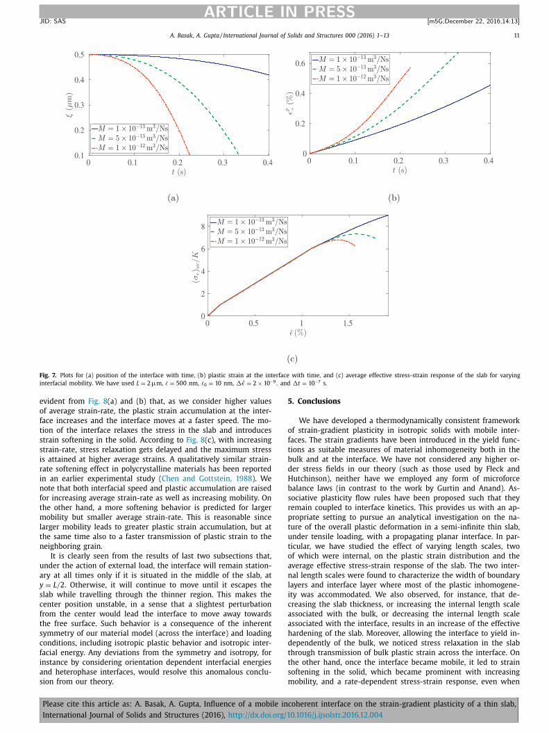
t al., 2001 ). For all our calculations we assume (εp + ) 0 = 10 −6 . Ac-
ording to Fig. 7 (a), as expected, interface propagates faster with
ncreasing mobility. There is no interface movement until it has
ielded. It is also clear from the plots that the interfacial speed
s sensitive to even small variations in the mobility; in fact, above
ertain values of mobility, it can move at very high speeds. We
ave not reported data after a point when interface is close to the
xternal boundary. At this point the interface might start to in-
eract with the boundary and can have a different response than
hat has been formulated in our work. With increasing mobil-
ty, the plastic strain accumulated at the interface also increases,
s has been shown in Fig. 7 (b). Therefore, one can relate speed of
he interface motion with plastic strain accumulation at the inter-
ace. A higher value of the latter also signifies higher incoherency
t the interface, which is equivalent to, e.g., high density of inter-
ace dislocations. The effect of mobility on the average stress-strain
esponse of the slab is shown in 7 (c). The stress-strain responses
re identical prior to interface yielding, but differ significantly af-
erwards. The average stress-strain response is increasingly non-
inear, with a well defined maxima, for higher values of interfa-
ial mobility. The interface propagation relaxes the stress in the
lab, more so for higher mobilities. This is evident in the soften-
ng response soon after interface yielding. In other words, a fast
oving interface would relax the stress more rapidly than a slower
ne. Such softening in polycrystalline materials, with average grain
ize of microns, sub-microns, and nano scales, has been reported
idely in the experimental literature ( Chen and Gottstein, 1988;
orris et al., 2007; Legros et al., 2008 ).
To obtain a different perspective from our formulation, we now
onsider the slab deformation to be instead controlled by prescrib-
ng displacements on the free boundary. In such a process, we fix
he value of the average strain-rate ˙ ε and calculate the load ac-
ordingly. We again plot interface position, plastic strain accumu-
ation, and stress-strain response of the slab for various values of
he average strain-rate. The mobility value is kept constant. It is
coherent interface on the strain-gradient plasticity of a thin slab,
0.1016/j.ijsolstr.2016.12.004
A. Basak, A. Gupta / International Journal of Solids and Structures 0 0 0 (2016) 1–13 11
ARTICLE IN PRESS
JID: SAS [m5G; December 22, 2016;14:13 ]
Fig. 7. Plots for (a) position of the interface with time, (b) plastic strain at the interface with time, and (c) average effective stress-strain response of the slab for varying
interfacial mobility. We have used L = 2 μm, � = 500 nm, � 0 = 10 nm, �ε = 2 × 10 −9 , and �t = 10 −7 s.
e
o
f
t
s
s
i
r
i
n
f
t
m
l
t
n
u
a
y
s
c
f
t
s
c
f
i
a
s
5
o
f
t
b
d
H
b
s
r
p
t
u
t
o
a
n
l
i
c
a
a
h
d
t
t
s
m
vident from Fig. 8 (a) and (b) that, as we consider higher values
f average strain-rate, the plastic strain accumulation at the inter-
ace increases and the interface moves at a faster speed. The mo-
ion of the interface relaxes the stress in the slab and introduces
train softening in the solid. According to Fig. 8 (c), with increasing
train-rate, stress relaxation gets delayed and the maximum stress
s attained at higher average strains. A qualitatively similar strain-
ate softening effect in polycrystalline materials has been reported
n an earlier experimental study ( Chen and Gottstein, 1988 ). We
ote that both interfacial speed and plastic accumulation are raised
or increasing average strain-rate as well as increasing mobility. On
he other hand, a more softening behavior is predicted for larger
obility but smaller average strain-rate. This is reasonable since
arger mobility leads to greater plastic strain accumulation, but at
he same time also to a faster transmission of plastic strain to the
eighboring grain.
It is clearly seen from the results of last two subsections that,
nder the action of external load, the interface will remain station-
ry at all times only if it is situated in the middle of the slab, at
= L/ 2 . Otherwise, it will continue to move until it escapes the
lab while travelling through the thinner region. This makes the
enter position unstable, in a sense that a slightest perturbation
rom the center would lead the interface to move away towards
he free surface. Such behavior is a consequence of the inherent
ymmetry of our material model (across the interface) and loading
onditions, including isotropic plastic behavior and isotropic inter-
acial energy. Any deviations from the symmetry and isotropy, for
nstance by considering orientation dependent interfacial energies
nd heterophase interfaces, would resolve this anomalous conclu-
ion from our theory.
Please cite this article as: A . Basak, A . Gupta, Influence of a mobile in
International Journal of Solids and Structures (2016), http://dx.doi.org/1
. Conclusions
We have developed a thermodynamically consistent framework
f strain-gradient plasticity in isotropic solids with mobile inter-
aces. The strain gradients have been introduced in the yield func-
ions as suitable measures of material inhomogeneity both in the
ulk and at the interface. We have not considered any higher or-
er stress fields in our theory (such as those used by Fleck and
utchinson), neither have we employed any form of microforce
alance laws (in contrast to the work by Gurtin and Anand). As-
ociative plasticity flow rules have been proposed such that they
emain coupled to interface kinetics. This provides us with an ap-
ropriate setting to pursue an analytical investigation on the na-
ure of the overall plastic deformation in a semi-infinite thin slab,
nder tensile loading, with a propagating planar interface. In par-
icular, we have studied the effect of varying length scales, two
f which were internal, on the plastic strain distribution and the
verage effective stress-strain response of the slab. The two inter-
al length scales were found to characterize the width of boundary
ayers and interface layer where most of the plastic inhomogene-
ty was accommodated. We also observed, for instance, that de-
reasing the slab thickness, or increasing the internal length scale
ssociated with the bulk, or decreasing the internal length scale
ssociated with the interface, results in an increase of the effective
ardening of the slab. Moreover, allowing the interface to yield in-
ependently of the bulk, we noticed stress relaxation in the slab
hrough transmission of bulk plastic strain across the interface. On
he other hand, once the interface became mobile, it led to strain
oftening in the solid, which became prominent with increasing
obility, and a rate-dependent stress-strain response, even when
coherent interface on the strain-gradient plasticity of a thin slab,
0.1016/j.ijsolstr.2016.12.004
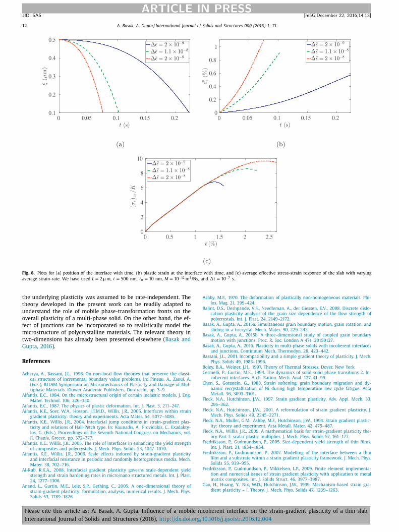
12 A. Basak, A. Gupta / International Journal of Solids and Structures 0 0 0 (2016) 1–13
ARTICLE IN PRESS
JID: SAS [m5G; December 22, 2016;14:13 ]
Fig. 8. Plots for (a) position of the interface with time, (b) plastic strain at the interface with time, and (c) average effective stress-strain response of the slab with varying
average strain-rate. We have used L = 2 μm, � = 500 nm, � 0 = 10 nm, M = 10 −12 m
3 /Ns, and �t = 10 −7 s.
A
B
B
B
B
C
F
F
F
F
G
the underlying plasticity was assumed to be rate-independent. The
theory developed in the present work can be readily adapted to
understand the role of mobile phase-transformation fronts on the
overall plasticity of a multi-phase solid. On the other hand, the ef-
fect of junctions can be incorporated so to realistically model the
microstructure of polycrystalline materials. The relevant theory in
two-dimensions has already been presented elsewhere ( Basak and
Gupta, 2016 ).
References
Acharya, A. , Bassani, J.L. , 1996. On non-local flow theories that preserve the classi-cal structure of incremental boundary value problems. In: Pineau, A., Zaoui, A.
(Eds.), IUTAM Symposium on Micromechanics of Plasticity and Damage of Mul-
tiphase Materials. Kluwer Academic Publishers, Dordrecht, pp. 3–9 . Aifantis, E.C. , 1984. On the microstructural origin of certain inelastic models. J. Eng.
Mater. Technol. 106, 326–330 . Aifantis, E.C. , 1987. The physics of plastic deformation. Int. J. Plast. 3, 211–247 .
Aifantis, K.E. , Soer, W.A. , Hosson, J.T.M.D. , Willis, J.R. , 2006. Interfaces within straingradient plasticity: theory and experiments. Acta Mater. 54, 5077–5085 .
Aifantis, K.E. , Willis, J.R. , 2004. Interfacial jump conditions in strain-gradient plas-
ticity and relations of Hall-Petch type. In: Kounadis, A., Providakis, C., Exadakty-los, G. (Eds.), Proceedings of the Seventh National Congress on Mechanics, vol.
II, Chania, Greece, pp. 372–377 . Aifantis, K.E. , Willis, J.R. , 2005. The role of interfaces in enhancing the yield strength
of composites and polycrystals. J. Mech. Phys. Solids 53, 1047–1070 . Aifantis, K.E. , Willis, J.R. , 2006. Scale effects induced by strain-gradient plasticity
and interfacial resistance in periodic and randomly heterogeneous media. Mech.Mater. 38, 702–716 .
Al-Rub, R.K.A. , 2008. Interfacial gradient plasticity governs scale-dependent yield
strength and strain hardening rates in micro/nano structured metals. Int. J. Plast.24, 1277–1306 .
Anand, L. , Gurtin, M.E. , Lele, S.P. , Gething, C. , 2005. A one-dimensional theory ofstrain-gradient plasticity: formulation, analysis, numerical results. J. Mech. Phys.
Solids 53, 1789–1826 .
Please cite this article as: A . Basak, A . Gupta, Influence of a mobile in
International Journal of Solids and Structures (2016), http://dx.doi.org/1
shby, M.F. , 1970. The deformation of plastically non-homogeneous materials. Phi-
los. Mag. 21, 399–424 . alint, D.S. , Deshpande, V.S. , Needleman, A. , der Giessen, E.V. , 2008. Discrete dislo-
cation plasticity analysis of the grain size dependence of the flow strength ofpolycrystals. Int. J. Plast. 24, 2149–2172 .
asak, A . , Gupta, A . , 2015a. Simultaneous grain boundary motion, grain rotation, andsliding in a tricrystal. Mech. Mater. 90, 229–242 .
Basak, A. , Gupta, A. , 2015b. A three-dimensional study of coupled grain boundarymotion with junctions. Proc. R. Soc. London A 471, 20150127 .
asak, A. , Gupta, A. , 2016. Plasticity in multi-phase solids with incoherent interfaces
and junctions. Continuum Mech. Thermodyn. 28, 423–442 . assani, J.L. , 2001. Incompatibility and a simple gradient theory of plasticity. J. Mech.
Phys. Solids 49, 1983–1996 . Boley, B.A. , Weiner, J.H. , 1997. Theory of Thermal Stresses. Dover, New York .
ermelli, P. , Gurtin, M.E. , 1994. The dynamics of solid-solid phase transitions 2. In-coherent interfaces. Arch. Ration. Mech. Anal. 127, 41–99 .
Chen, S. , Gottstein, G. , 1988. Strain softening, grain boundary migration and dy-
namic recrystallization of Ni during high temperature low cycle fatigue. ActaMetall. 36, 3093–3101 .
leck, N.A. , Hutchinson, J.W. , 1997. Strain gradient plasticity. Adv. Appl. Mech. 33,295–362 .
leck, N.A. , Hutchinson, J.W. , 2001. A reformulation of strain gradient plasticity. J.Mech. Phys. Solids 49, 2245–2271 .
Fleck, N.A. , Muller, G.M. , Ashby, M.F. , Hutchinson, J.W. , 1994. Strain gradient plastic-
ity: theory and experiment. Acta Metall. Mater. 42, 475–487 . Fleck, N.A. , Willis, J.R. , 2009. A mathematical basis for strain-gradient plasticity the-
ory-Part I: scalar plastic multiplier. J. Mech. Phys. Solids 57, 161–177 . Fredriksson, P. , Gudmundson, P. , 2005. Size-dependent yield strength of thin films.
Int. J. Plast. 21, 1834–1854 . redriksson, P. , Gudmundson, P. , 2007. Modelling of the interface between a thin
film and a substrate within a strain gradient plasticity framework. J. Mech. Phys.
Solids 55, 939–955 . redriksson, P. , Gudmundson, P. , Mikkelsen, L.P. , 2009. Finite element implementa-
tion and numerical issues of strain gradient plasticity with application to metalmatrix composites. Int. J. Solids Struct. 46, 3977–3987 .
ao, H. , Huang, Y. , Nix, W.D. , Hutchinson, J.W. , 1999. Mechanism-based strain gra-dient plasticity – I. Theory. J. Mech. Phys. Solids 47, 1239–1263 .
coherent interface on the strain-gradient plasticity of a thin slab,
0.1016/j.ijsolstr.2016.12.004
A. Basak, A. Gupta / International Journal of Solids and Structures 0 0 0 (2016) 1–13 13
ARTICLE IN PRESS
JID: SAS [m5G; December 22, 2016;14:13 ]
G
G
G
G
G
G
G
H
H
M
K
K
K
L
M
N
N
P
P
P
R
S
S
V
W
W
W
Z
Z
Z
orkaya, T. , Molodov, K.D. , Molodov, D.A. , Gottstein, G. , 2011. Concurrent grainboundary motion and grain rotation under an applied stress. Acta Mater. 59,
5674–5680 . ourdet, S. , Montheillet, F. , 2002. Effects of dynamic grain boundary migration dur-
ing the hot compression of high stacking fault energy metals. Acta Mater. 50,2801–2812 .
udmundson, P. , 2004. A unified treatment of strain gradient plasticity. J. Mech.Phys. Solids 52, 1379–1406 .
upta, A. , Steigmann, D.J. , 2012. Plastic flow in solids with interfaces. Math. Meth-
ods Appl. Sci. 35, 1799–1824 . urtin, M.E. , Anand, L. , 2005. A theory of strain-gradient plasticity for isotropic,
plastically irrotational materials. part I: small deformations. J. Mech. Phys. Solids53, 1624–1649 .
urtin, M.E. , Anand, L. , 2009. Thermodynamics applied to gradient theories in-volving the accumulated plastic strain: the theories of Aifantis and Fleck and
Hutchinson and their generalization. J. Mech. Phys. Solids 57, 405–421 .
urtin, M.E. , Jabbour, M.E. , 2002. Interface evolution in three dimensions with cur-vature-dependent energy and surface diffusion: interface-controlled evolution,
phase transitions, epitaxial growth of elastic films. Arch. Ration. Mech. Anal.163, 171–208 .
osson, J.T.M.D. , Soer, W.A. , Minor, A.M. , Shan, Z. , Stach, E.A. , Asif, S.A.S. , War-ren, O.L. , 2006. In situ TEM nanoindentation and dislocation-grain boundary in-
teractions: a tribute to David Brandon. J. Mater. Sci. 41, 7704–7719 .
uang, Y. , Gao, H. , Nix, W.D. , Hutchinson, J.W. , 20 0 0. Mechanism-based strain gra-dient plasticity – II. Analysis. J. Mech. Phys. Solids 48, 99–128 .
orris Jr., J.W. , Jin, M. , Minor, A.M. , 2007. In situ studies of the transmission of strainacross grain boundaries. Mater. Sci. Eng. A 462, 412–417 .
ochmann, D.M. , Le, K.C. , 2008. Dislocation pile-ups in bicrystals within continuumdislocation theory. Int. J. Plast. 24, 2125–2147 .
rishnan, J. , Steigmann, D.J. , 2014. A polyconvex formulation of isotropic elastoplas-
ticity theory. IMA J. Appl. Math. 79, 722–738 . röner, E. , et al. , 1981. Continuum theory of defects. In: Balian, R., et al. (Eds.), Les
Houches, Session XXXV, 1980 –Physique des Défauts. North-Holland PublishingCompany, pp. 215–315 .
egros, M. , Gianola, D.S. , Hemker, K.J. , 2008. In situ TEM observations of fastgrain-boundary motion in stressed nanocrystalline aluminum films. Acta Mater.
56, 3380–3393 .
Please cite this article as: A . Basak, A . Gupta, Influence of a mobile in
International Journal of Solids and Structures (2016), http://dx.doi.org/1
azzoni-Leduc, L. , Pardoen, T. , Massart, T.J. , 2008. Strain gradient plasticity analysisof transformation induced plasticity in multiphase steels. Int. J. Solids Struct. 45,
5397–5418 . oll, W. , 1967. Materially uniform simple bodies with inhomogeneities. Arch. Ration.
Mech. Anal. 27, 1–32 . ye, J.F. , 1953. Some geometrical relations in dislocated crystals. Acta Metall. 1,
153–162 . ardoen, T. , Massart, T.J. , 2012. Interface controlled plastic flow modelled by strain
gradient plasticity theory. C.R. Mec. 340, 247–260 .
olizzotto, C. , 2009. Interfacial energy effects within the framework of strain gradi-ent plasticity. Int. J. Solids Struct. 46, 1685–1694 .
uri, S. , Das, A. , Acharya, A. , 2011. Mechanical response of multicrystalline thin filmsin mesoscale field dislocation mechanics. J. Mech. Phys. Solids 59, 2400–2417 .
upert, T.J. , Gianola, D.S. , Gan, Y. , Hemker, K.J. , 2009. Experimental observations ofstress-driven grain boundary migration. Science 326, 1686–1690 .
hu, J.Y. , Fleck, N.A. , 1999. Strain gradient crystal plasticity: size dependent defor-
mation of bicrystals. J. Mech. Phys. Solids 47, 186–213 . utton, A.P. , Balluffi, R.W. , 2003. Interfaces in Crystalline Materials. Clarendon Press,
Oxford . oyiadjis, G.Z. , Faghihi, D. , Zhang, Y. , 2014. A theory for grain boundaries with
strain-gradient plasticity. Int. J. Solids Struct. 51, 1872–1889 . inning, M. , Gottstein, G. , Shvindlerman, L.S. , 2001. Stress induced grain boundary
motion. Acta Mater. 49, 211–219 .
ulfinghoff, S. , Bayerschen, E. , Böhlke, T. , 2013. A gradient plasticity grain boundaryyield theory. Int. J. Plast. 51, 33–46 .
ulfinghoff, S. , Forest, S. , Böhlke, T. , 2015. Strain gradient plasticity modeling of thecyclic behavior of laminate microstructures. J. Mech. Phys. Solids 79, 1–20 .
hang, X. , Aifantis, K.E. , 2015. Examining the evolution of the internal length as afunction of plastic strain. Mater. Sci. Eng., A 631, 27–32 .
hang, X. , Aifantis, K.E. , Ngan, A.H.W. , 2014a. Interpreting the stress-strain response
of Al micropillars through gradient plasticity. Mater. Sci. Eng. A 591, 38–45 . hang, X. , Aifantis, K.E. , Senger, J. , Weygand, D. , Zaiser, M. , 2014b. Internal length
scale and grain boundary yield strength in gradient models of polycrystal plas-ticity: how do they relate to the dislocation microstructure? J. Mater. Res. 29,
2116–2128 .
coherent interface on the strain-gradient plasticity of a thin slab,
0.1016/j.ijsolstr.2016.12.004


![Interface evolution in three-dimensions with curvature …€¦ · tional moments introduced by DiCarlo, Gurtin & Podio-Guidugli [1992]. 9Inertial e ects are easily included. Cf.,](https://img.pdfslide.us/doc/110x75/5b446ff57f8b9ae0668bb4c5/interface-evolution-in-three-dimensions-with-curvature-tional-moments-introduced.jpg)
![ychen11/PUBLICATIONS/[12].pdfI. Introduction 175 One of the cornerstones of kinematics in continuum mechanics is the polar ... M.E Gurtin, Introduction to Continuum Mechanics](https://img.pdfslide.us/doc/110x75/5af062f87f8b9ac57a8e8747/ychen11publications12pdfi-introduction-175-one-of-the-cornerstones-of-kinematics.jpg)


![UNCLASSI]I ED A D 402! 2I 2 - dtic.milI ED A D 402! 2I 2 ... IN CONTINUUM MECHANICS by M. E. Gurtin SiA APR? TIv 25 ... M. E. Gurtin Brown riUniversity 1. Introduction](https://img.pdfslide.us/doc/110x75/5af062f87f8b9ac57a8e871b/unclassii-ed-a-d-402-2i-2-dtic-i-ed-a-d-402-2i-2-in-continuum-mechanics.jpg)


![LINEARIZATION - CaltechAUTHORS · The linear theory can also be developed on a separate footing, as in Gurtin [1972a]. Often, linearization of the equations of continuum mechanics](https://img.pdfslide.us/doc/110x75/5b446d8d7f8b9a56348b5245/linearization-caltechauthors-the-linear-theory-can-also-be-developed-on-a.jpg)