Embed Size (px)
Citation preview

Article
Development of Occupant-Preferred Landing Profiles for Personal Aerial Vehicles
Lu, Linghai and Jump, M
Available at http://clok.uclan.ac.uk/14073/
Lu, Linghai ORCID: 0000-0002-2688-7944 and Jump, M (2016) Development ofOccupant-Preferred Landing Profiles for Personal Aerial Vehicles. Journal of Guidance, Control, and Dynamics, 39 (8). pp. 1805-1819. ISSN 0731-5090
It is advisable to refer to the publisher’s version if you intend to cite from the work.http://dx.doi.org/10.2514/1.G001608
For more information about UCLan’s research in this area go to http://www.uclan.ac.uk/researchgroups/ and search for <name of research Group>.
For information about Research generally at UCLan please go to http://www.uclan.ac.uk/research/
All outputs in CLoK are protected by Intellectual Property Rights law, includingCopyright law. Copyright, IPR and Moral Rights for the works on this site are retainedby the individual authors and/or other copyright owners. Terms and conditions for useof this material are defined in the policies page.
CLoKCentral Lancashire online Knowledgewww.clok.uclan.ac.uk
Development of Occupant-Preferred Landing Profiles for Personal Aerial Vehicles
Linghai Lu 1, Michael Jump 2, Mark White3 and Philip Perfect4 Centre for Engineering Dynamics, University of Liverpool, Liverpool, UK, L69 3BX
With recent increased interest in autonomous vehicles and the associated technology, the
prospect of realizing a personal aerial vehicle (PAV) seems closer than ever. However, there
is likely to be a continued requirement for any occupant of an air vehicle to be comfortable
with both the automated portions of the flight and their ability to take manual control as and
when required. This paper, using the approach to landing as an example maneuver, examines
what a comfortable trajectory for PAV occupants might look like. Based upon simulated flight
data, a ‘natural’ flight trajectory was designed and then compared to constant deceleration
and constant optic flow descent profiles. It was found that PAV occupants with limited flight
training and no artificial guidance followed the same longitudinal trajectory as had been
found for professionally trained helicopter pilots. Further, the final stages of the approach to
hover could be well described using Tau Theory. For automatic flight, PAV occupants
preferred a constant deceleration profile. For approaches flown manually, the newly designed
natural profile was preferred.
Nomenclature
ax, az = acceleration in the x and z axis, ft/s2
axc = longitudinal commanded acceleration, ft/s2
axd = commanded acceleration to drive this symbology, ft/s2
c, C = constant parameters
k = coupling constant
1 Research Associate, Centre for Engineering Dynamics, and now Lecturer in the University of Central Lancashire, Email: [email protected]; AIAA Member. 2 Senior Lecturer, Centre for Engineering Dynamics, Email: [email protected]; AIAA Member 3 Lecturer, Centre for Engineering Dynamics; Email: [email protected] 4 Research Associate, Centre for Engineering Dynamics, now with Blue Bear Systems Research.

ka, kd = coupling constants for constant acceleration and deceleration
kf = tangent value of the constant flight path angle
kr = coupling constant for flight path guidance
kr = gain to account for the velocity difference
Kg = collective input to the command flight path angle
KI, Kp = integral and proportional gains
g = acceleration of gravity, ft/s2
h = instantaneous height above the ground, ft
m, n = number of ratings given by each test subject
p = number of the current profile
t = time, s
t = normalized by the maneuver period
T = maneuver period, s
Tr = flight path arising period, s
u = forward velocity in the body axis, ft/s
x, y, z = pilot's viewpoint distance ahead and lateral of the aircraft and height above the ground, ft
x , x = closure rate and acceleration to a boundary (x-axis), ft/s, ft/s2
z , z = closure rate and acceleration to a boundary (z-axis), ft/s, ft/s2
Zw,col
Z = collective heave and control damping derivatives
γa, a = flight path angle gap to go and gap closure rate, deg, deg/s
γf = final flight patch angle, deg
δcol, δlon = collective and longitudinal control input, inch
η = pilot’s control deflection, inch
pk = peak of the rate of control input, inch/s
τ = instantaneous time to contact boundary in the optical field, s
g = intrinsic τ guidance, s
d = time delay between the cyclic input and acceleration response, s
= rate change of optical tau
ω = eye height velocity, 1/s
I. Introduction
lobal interest in autonomous vehicles continues apace, with the introduction of some form of automatically driven
or autonomous ‘car’ seeming increasingly likely with 5 – 10 years [1-3]. However, within that community, there is
still intense debate concerning the role of the human operator. Thinking further ahead, it is conceivable that these
technologies could also be used to finally realize the concept of a personal aerial vehicle (PAV). Given the more
stringent regulatory framework that exists around current aviation technology, it is likely that the requirement for the
human operator to be able to intervene will exist. Indeed, current thinking around unmanned aircraft is that, to remain
within current regulations, a remote pilot will always need to be in command [1-3]. A truly autonomous aircraft i.e.
an aircraft that does not allow human intervention in a flight [4] will not be able to be integrated into the current
airspace framework in the foreseeable future as it would not conform with Article 8 of the Chicago Convention [4].
On the reasonable assumption that PAVs will not be remotely operated i.e. the pilot is located somewhere other than
the vehicle itself, the operator of a PAV must, therefore, be ‘in the loop’ and be capable of intervening effectively. It
is anticipated then, that some form of trajectory guidance assistance will be required in the case of PAVs being
operated by their human occupants. These PAV occupants will generally not be professionally-trained pilots. Phases
of flight close to the ground will be of most concern in terms of the ability of the occupants to both follow and accept
the required vehicle trajectories. It is these phases of flight, and specifically the landing approach, that is the focus of
this paper.
Guidance for the landing approach maneuver for professional pilotage has evolved over the period of modern
manned aviation. The use of the ubiquitous instrument landing system localizer and glideslope indicators provides the
pilot with precision lateral and vertical guidance cueing to assist with the task of flying the aircraft along a prescribed
flight path down to the runway. Primarily in use in military aircraft, the conformal flight-path vector symbol on a
head-up display (HUD) allows the pilot to place that symbol on the runway threshold to achieve the same outcome in
visual meteorological conditions. For private pilots, such technologies are not necessarily available. This is either
because the aircraft is not suitably equipped or because they are not qualified to use them. One technique that is
therefore employed to fly the correct trajectory is to pick a reference point (the runway threshold markers, for
G

example), and to ensure that this reference maintains its position in the windshield in the pilot’s field of view down
the approach path.
For future civilian aerial operations, the European Commission’s Framework VI project, ‘OPTIMAL’ [4], focused
on defining and validating innovative solutions for the approach and landing phases of both fixed- and rotary-wing
aircraft to deliver greater airport capacity, improved transport efficiency, reduced environmental impact and increased
safety. This project differs from the results of the current study. First, OPTIMAL developed state-of-the-art trajectories
using both new and existing precision instrument landing aids as well as new Air Traffic Management technologies.
The research in the current paper develops profiles that are based upon the available visual information from outside
the cockpit. Second, the innovative approach and landing methodologies developed in the OPTIMAL project are
intended for use by highly trained, highly motivated professional pilots. For the present research, the subjects of
interest are not professional pilots. Third, the present work concentrates on the comfort of the PAV occupant which is
not a feature of the OPTIMAL project.
It is anticipated that the more intuitive and salient the perceptual information provided to the occupant of a PAV
is, the greater will be their ability to make rationale and correct decisions regarding control of the aircraft. It is proposed
in Ref. [5;6] that a future PAV will require a hover capability. PAVs may therefore share some similarities, in terms
of allowable trajectories, with modern rotary-wing aircraft. Numerous previous studies have been undertaken to
understand rotary-wing pilot control behavior during a visual landing task [7]. Some of the salient pioneering research
was conducted by NASA during a study to design a flight director system to provide an approach profile based upon
“natural physiological" cueing [8-13]. The characteristic shapes of 236 professionally- piloted visual approaches using
four helicopter types and nine sets of initial conditions were analyzed. The altitude, ground-speed, and deceleration
profiles of the visual approaches were thus mathematically determined. The following kinematic relationship for the
deceleration phase in the horizontal (x)-axis resulted from the analysis of the flight-test results:
2
n
cxx
x (0)
in which c and n are constants. The results have been verified by flight simulation trials at the UoL [10] and by
Heffley's mathematical model of the human operator [14].
For helicopter visual approaches, pilots are trained to maintain a constant optical flow (OF) during the approach
to landing [8]. Guidance using OF is also widely reported to be used in both the animal kingdom [15] and in

autonomous robotic systems [16]. More recently, the research of Ref. [17-19] proposed an improved deceleration
guidance cueing system within the Brown-Out Symbology Simulation (BOSS) display to provide the pilot with
intuitive guidance cues to enable the safe landing of a rotorcraft in brownout, zero-visibility conditions. This
comprised a hybrid profile, consisting of constant deceleration (CD) and constant OF phases of flight.
If PAVs were to become a widely-used transportation method, the expectation is that the ‘piloting’ of them should
demand no more skill than that associated with driving a car today [20]. Therefore, it would be expected that the
number of hours of training received by a novice PAV ‘pilot’ would be lower than that currently required to gain and
maintain a Private Pilot’s License (PPL) – a level that might be termed ‘flight naïve’. It is not expected that the general
public will all become private pilots, rather, that different ‘modes’ of operation might be employed, ranging from
‘manual’, with ‘highly augmented’ flight control to ‘fully automatic’ flight, perhaps leading to a new licensing
category specifically for PAV pilots. For the maneuvers where a manual mode was available, it would be of interest
to design a flight trajectory to provide cueing that is as "natural" as possible. Such cues would be indicated to the pilot
by some kind of flight director system. Such a system would need to ensure that the PAV and its occupants followed
the desired trajectory in a safe manner [7]. For automated flight, it is further anticipated that, to allow the human
operator to intervene quickly, the automated trajectories would need to be, in some way, what the operator is both
expecting and is comfortable with. The question therefore arises as to whether the trajectory guidance provided for a
given maneuver needs to be the same for the cases where a PAV is being flown either automatically or manually. This
paper addresses these questions, using the landing approach as the exemplar maneuver.
The methodology described in this paper will draw heavily on the use of tau () theory. This theory is based upon
the premise that purposeful actions are accomplished by coupling the motion under control with either externally or
internally perceived motion variables – the so-called motion guides [21]. Motivated by its basis in visual perception,
researchers have applied tau to both flight control and handling qualities problems [20]. The hypothesis here is that,
in terms of a visual guidance strategy, the overall pilot’s goal is to overlay or close the gap between the perceived
optical flow-field and the required flight trajectory. For manual flight, the pilot then works directly with the available
optical variables to achieve prospective control of the aircraft’s future trajectory. For automated flight, the observer
must be comfortable that the available visual gaps are being closed in a manner such that the future vehicle trajectory
corresponds to their expectations.

The paper proceeds as follows. First, a brief resume of the associated theories being used is presented. Second, the
experimental setup used to gather approach trajectory data flown by flight-naïve participants is introduced. Third, the
paper then focuses on the development of an approach profile based upon the flight-naïve participant’s performance.
Fourth, the designed profile is evaluated by comparing it with two popular guidance methodologies using both
automatic and manual flight. Finally, a set of conclusions draw the paper to a close.
II. Theory
The following Section defines the relevant theory used to understand and construct the different approach profiles
used as part of the associated experimental test campaign.
A. The Eye-Height Scale
The eye-height scale is used to derive body-scaled information about the environment during motion [22-24]. It is
particularly convenient to derive the visual and motion cues available to a pilot in the optical flow field using this
scale. Recent research indicates that this scale can be used as a ‘perspective index’ to characterize how and when pilots
know when to stop, turn or pull up [25]. Fig. 1 illustrates the parameters used when describing flight in terms of eye-
heights.
Fig. 1 Illustration of the parameters used to compute eye-height distance
The eye-height distance can then be simply computed as follows:
Eye Heightz
x (0)
in which x and z are the pilot's viewpoint distance ahead of the aircraft and instantaneous height above the ground,
respectively.
B. Constant Deceleration Kinematics

The CD profile algorithm adopts a CD value (ax) that can be determined using Eq. (0) in the longitudinal axis
during the whole maneuver,
20
02x
x
Va
x (0)
in which x0 is the initial distance to the end of the maneuver and Vx0 is the initial ground speed. Therefore, the
longitudinal position (x) at any time t is given by,
20 0.5x xx V t a t (0)
The forward velocity (Vx) and the total maneuver period (T) can also be determined. The vertical velocity (Vz) is
then defined by maintaining the flight path angle (γ),
tanz xV V (0)
C. Constant Optical Flow Kinematics
The optical flow of a point in the scene directly ahead (ω, the velocity in eye-heights per second) perceived by a
subject during the flight is given by Ref. [26-28],
xV
h (0)
where Vx is the ground speed and h is the instantaneous height above the ground. With an assumed constant flight path
angle, , the position information in the x-axis can be derived as follows,
tan0
tx x e (0)
The Vx information as well as the speed and position information in the vertical axis can then be derived from Eq.
(0) for a fixed flight path angle. As shown in Eq. (0), a PAV being flown with a constant OF profile approaches the
target at an exponentially decreasing rate with respect to time. In theory at least, following such a trajectory, the vehicle
will never reach the destination. Pilots have been found to adapt their control strategies when following exponential
trajectories to avoid this problem in, for example, Ref. [13].
D. Optical Tau Theory
The following provides a brief overview of tau theory as it pertains to flight control. For a more complete
description, see Ref. [29]. Optical tau (τ), the time-to-contact variable, in the optical field is defined in Eq. (0),

x
x
x
(0)
It has been constructed using the conceptual framework for understanding information used in detecting an
upcoming collision [25], where x is the motion gap to be closed and x is the instantaneous gap closure rate. The term
‘motion gap’ refers to a perceived difference between the observer’s current and desired target state.
Tau theory further hypothesizes that the observer’s motion is guided using coupling. Here the tau of one motion
gap is kept in constant ratio with the tau of another motion gap. In practice, there are often two or more gaps that need
to be closed simultaneously, such as the coordination required between lateral and forward motions, or forward and
vertical motions, in order to achieve combined horizontal-vertical maneuvers [15;27-29]. Two motions, x(t) and z(t),
are said to be tau-coupled if the following relationship is satisfied,
z xk (0)
The coupling term k in Eq. (0) regulates the dynamics of the motions in the x and z directions in this specific
example. If a second externally perceivable motion gap is not available, it is hypothesized that self-guided motion can
still be achieved by coupled onto an intrinsic motion guide, g. Intrinsic τ guidance is modeled using the relationship,
x gk (0)
in which g can take the form of constant deceleration (with coupling term kd) for deceleration-to-stop motions (e.g.,
car braking [22;30] and prospective guidance in a fixed-wing aircraft flare maneuver [31]) or constant acceleration
(with coupling term ka) for acceleration-deceleration motions (e.g., prospective guidance in a stopping maneuver [30]).
The analysis of vehicle motion therefore comes down to selecting an appropriate motion gap or gaps:
gap finalx x x (0)
where ‘x’ is the current value of the motion parameter and ‘xfinal’, for the purposes of this paper, is the value of x when
0finalx . The motion gap profile can be compared to the motion of the appropriate tau guide. The coupling constant,
k, and total maneuver time, ‘T’ that define the motion can then be computed using the method shown in Ref. [29].
E. The Attack Parameter
A pilot’s workload can be measured by calculating the control attack parameter which measures the size and
rapidity of a pilot’s control inputs [32], defined as,

pkattack
(0)
where η is the pilot’s control deflection and pk is the peak of the rate of control input. The number of times that a
pilot moves a particular control can be used to describe the pilot’s control activity (the attack number).
III. Experimental Set-Up
The results presented in this paper arise from the conduct of two distinct but related test campaigns. Both of these
are described in this Section.
A. Flight Simulation Facility
Both of the test campaigns reported in this paper were conducted in the HELIFLIGHT-R simulator shown in Fig.
2 (Ref. [33]). The simulator was configured as described in Ref. [14].
Fig. 2 External and interior views of the HELIFLIGHT-R flight simulator
B. PAV Flight Dynamics Model
The PAV flight dynamics model used for the experiments described in this paper is the ‘Hybrid’ model reported
in Refs. [34]. This model was configured to give excellent handling qualities for non-professional pilots with a wide
range of flying aptitudes. It is equipped with the ability to hover. However, it is not anticipated that PAVs will exhibit
any significant helicopter-like control cross-couplings by design and so, unlike a conventional helicopter, its off-axis
responses are decoupled i.e. there is no response in the roll axis to a longitudinal axis input and vice-versa. For the
experiments conducted, conventional helicopter cyclic and collective controls were used. The novice PAV pilots were

instructed in the use of the collective control to command flight path angle and the longitudinal cyclic to control
forward speed.
C. Experimental Flight Test Maneuver Description
The PAV commuting mission, described in Ref. [7;34], was broken down into a number of Mission Task Elements
following the method of Ref. [7]. The decelerating-descent MTE is the one that relates to the landing approach. A
schematic of the entire maneuver course is shown in Fig. 3a and a zoomed-in schematic of the final hover position is
shown in Fig. 3b [21].
Fig. 3 Description of decelerating descent maneuver a.) General arrangement; b.) Enlarged hover board
The maneuver shown in Fig. 3a begins with the aircraft in a stable, straight and level cruise at a forward speed of
60 kts, at a height of 500 ft above ground level (AGL) and 4500 ft from the desired hover position. The descent begins
as the aircraft passes over the first runway threshold in the visual scene. This approach profile results in a mean glide
slope angle of -6 degrees. The original lateral track and heading had to be maintained during the maneuver. The
maneuver was completed once a stabilized hover was achieved at a height of 20 ft AGL within pre-defined lateral and
longitudinal ground positions (Fig. 3b).
D. Exploratory Visual Approaches
The first experiment was conducted to allow potential PAV pilots to fly a series of visual approaches to ascertain
what their preferred trajectory might be. To be able to do this, the participants were given basic instruction on the
function of the control inceptors and the displays available to them. The test campaign involved 11 test subjects (TSs)
who were not professional pilots (10 male, 1 female, with an age range of 20-43 and a mean age of 26). The TSs were
broadly categorized by their prior flight experience: No Flying Experience, Simulator Flying Experience only, and

Flight Experience (to Private Pilot level). In addition, for this purely visual landing task, the subjects were instructed
to fly the maneuver to comply with the requirements in Fig. 3a, with recourse only to the outside world visual cueing
provided. All TSs were required to repeat each test maneuver at least three times. Data-gathering test runs were only
conducted once a number of familiarization runs had been completed by each test subject. The number of
familiarization runs used was varied based upon both the participant’s previous flight experience and observed
aptitude/competence on the day (in terms of being able to achieve the task to at least an adequate level).
E. Enhanced Guidance Approaches
As previously stated, for the initial stage of the research, the approach task was flown purely with reference to the
outside world visual cues. Based upon these flights, an idealized approach trajectory was developed. The same group
of TSs (with one exception due to availability - the female TS was replaced by a male participant with simulator flying
experience) was asked to fly the approach task once again, but this time using some basic guidance symbology. The
guidance symbology was driven using various algorithms to generate the required trajectories. Specifically,
approaches were flown using a new trajectory design (reported later in the paper), a CD approach, and an approach
profile generated utilising constant OF. This series of simulated flights were then repeated with the vehicle under
automatic control i.e. the TSs were passive ‘passengers’. The order of the three profiles was randomised for each TS
to try to avoid any bias due to learning. For the automated flight test points, only outside-world visual cues were
provided.
1. Guidance Display for Manual Flight
For the assessment of the manually flown approach trajectories, the TSs were provided with the HUD guidance
symbols as illustrated in Fig. 4. The symbols have been arranged for clarity in the Figure.

Fig. 4 Head up display used for PAV manual landing tasks
Airspeed, heading, and radar altitude were provided in the numeric readout section. The airspeed indicated on the
left is the current commanded velocity. The airspeed indicated on the right shows the current actual velocity. The
Malcolm horizon line [21;34] was provided across the full field of view of the simulator. The HUD symbology also
included a flight path vector symbol and an attitude indicator. To provide inceptor guidance control information to the
TSs, two symbols were provided. The first was a ball (filled) and circle symbol, shown to the right of the display. The
circle showed the required position of the longitudinal cyclic for the current descent profile, whilst the ball indicated
the current actual position. To follow the desired trajectory, the TSs were required to maintain the ball within the circle
which moved up and down the vertical bar shown. The information (axd) used to drive this symbology is given by,
( )d sxd xc x x xca a e k V V (0)
in which axc and Vxc are the longitudinal commanded acceleration and velocity respectively. Vx is the current PAV
forward velocity. The first term on the right-hand side of Eq. (0) provided the acceleration information to drive the
circle symbol. The term τd was introduced to compensate for the time delay between the cyclic input and the vehicle’s
acceleration response, to increase the symbol tracking accuracy. The second term on the right-hand side of Eq. (0)
contains the difference between the actual and commanded velocities with a gain kx. This term removed the observed
velocity drift that following the acceleration command alone induced.
The second symbol-set used was the graphical highway-in-the-sky (HITS) flight path display system [35]. This
intuitive cockpit display shows the desired trajectory by way of “tunnel” in the visual scene ahead that the aircraft
must follow to maintain the desired Earth-referenced lateral and vertical positions. The inner brackets defined the

MTE desired performance requirements and the outer black brackets defined the MTE adequate performance
requirements for the maneuver.
2. Subjective Assessment Method
After three attempts had been made for each descent profile for both the automatic and manual flight cases, the
TSs were asked to provide subjective assessments using the Comfort and Presence questionnaire, shown in
Appendices A1 and A2. These two scales were developed in collaboration with the Faculty of Psychology, Health and
Society at the University of Liverpool.
IV. Results
A. Design of an Idealized Approach Trajectory
The first objective of this study was to design a landing profile that felt both natural and comfortable to PAV
occupants. The start point for this exercise was to observe how the TSs undertook the landing maneuver using only
the outside − world visual cues available to them. Fig. 5 shows the velocity and flight path angles from the trajectories
achieved by the 11 subjects against the longitudinal distance along the test course. The associated control inputs are
shown in Fig. 6. Only the final attempt at the task made by the TSs is shown in the Figures for clarity.
Vx,
ft/s
Vz,
ft/s
,deg
P1 P2 P3
No ExperienceSimulator ExperienceFlight Experience
a.)
b.)
c.) x, ft
Fig. 5 Body velocity and flight path angles achieved by 11 test subjects during the landing maneuver

Fig. 6 Longitudinal and collective inputs introduced by 11 test subjects
The test course, shown in Fig. 3, should have been initiated as the first runway threshold is crossed (x = 0 ft). It is
complete when a stable hover is achieved at the hover board (x = 4500 ft). However, as shown in Fig. 5c and Fig. 6b,
seven of the TSs initiated some form of change to the vehicle flight path angle some 300 ft ahead of the runway
threshold (where ≠ 0 at x < 0 ft in Fig. 5c). What is clear from the Figures is that three phases of guidance control
are discernible for each of the TS’s descent profiles. The initial phase (P1) of the maneuver only involves flight path
control. This can be seen from the almost constant forward velocity (Vx) in Fig. 5a (with negligible longitudinal control
inputs indicated in Fig. 6a) and the sharp change of the flight path angles in Fig. 5c (and also the collective control
inputs of Fig. 6b) during this period. The second distinct phase (P2) of the descent profile is distinguished by a change
in both the forward and vertical vehicle body velocities. The test subjects attempt to maintain the flight path angle
profiles (Fig. 5c and Fig. 6b) for a certain period before initiating the deceleration phase for the remaining part of the
maneuver. This indicates that the subjects adopt a constant flight path angle during this part of the maneuver. Finally,
Fig. 5c shows that, as the landing point is approached, maintaining a constant flight path angle is no longer the
desirable strategy. Intensive activity is evident in Fig. 6 in both control channels in this phase (P3).
Based upon these observations, each phase was scrutinized more closely to allow the profile to be generalized for
use in the second part of the study.

1. P1: First Phase - Flight Path Angle Control
An important feature in the early stage of the landing process shown in Fig. 6 is that flight path control was
performed using only the collective, with only minor longitudinal control inputs being performed to maintain the
desired speed. Given that none of the TSs were professional (helicopter) pilots, it is possible that they preferred to
focus on using only one control axis at a time for the landing maneuver. This was helped, of course, by the fact that
the collective control of the PAV model used in this project was completely decoupled from the other axes. The TSs
also commented that, due to the length of the test course, the final landing marker was barely visible. As such the TS
preferred to maintain their initial forward speed to avoid having to make abrupt longitudinal cyclic control inputs to
correct errors introduced at an early stage later in the maneuver. This kind of operation is consistent with normal
helicopter operational procedures for the final approach to a runway [36] whereby the descent is commenced by
selecting a recommended vertical speed.
In relation to τ theory then, there is only one motion gap to be closed in this phase i.e. the flight path angle, which
starts with a zero value and ends with some fixed value. This indicates that the flight path motion gap closure would
be most suitably modelled using a constant acceleration tau guide velocity profile. Fig. 7 shows the average Phase 1
period TP1, the final flight path angle achieved at the end of Phase 1, γf, and the tau guide coupling constant kr values
determined for the 11 subjects.
1 2 3 4 5 6 7 8 9 10110
5
10
15
20
25
Ris
e T
ime
Tr,
s
Subjects1 2 3 4 5 6 7 8 9 1011
0
5
10
15
Subjects
f,de
g
1 2 3 4 5 6 7 8 9 10110
0.1
0.2
0.3
0.4
0.5
Subjects
k
1 11.5 PT s 6.7 degf 1 0.19Pk
Fig. 7 Phase period, final flight path angle, and coupling term values obtained from the simulated flight trials
The Phase 1 period values in Fig. 7 range from 9 to 13s, with the exception of Subject 9 (the only female) where
the value is 18s. The γf values vary from 5.4 to 8.2 deg. The kγ values range from 0.13 to 0.26. The mean values

obtained are indicated in Fig. 7 with a bar. They were used to determine the γa profile as shown in Eq. (0) derived
from Eq. (0), using the intrinsic constant acceleration guide.
11/2 21( ) Pk
a PC T t (0)
in which C is a constant parameter. The resultant γa profile is compared with those of the actual data in Fig. 8.
-1 -0.8 -0.6 -0.4 -0.2 0-10
-8
-6
-4
-2
0
t
,deg
a
Fig. 8 Comparison of γa profiles between the actual data and the derived using the intrinsic constant
acceleration guide
The good ‘fit’ between the derived γa profile and the actual data supports the methodology used above. The γa
information can be further validated by a comparison of the derived τ-coupled collective inputs and the actual subject
inputs. To accomplish this validation, the simplified flight path control loop used in the PAV model [15;22;24;29;30]
is illustrated in Fig. 9.
Kg Kp
KI1
s
+ ++
col
w
Z
s Z
w
uatan
w
γ
col
Fig. 9 Flight path angle loop with collective control (Vx > 25kts)
in which Kg (= 30) is the control gearing from the collective input to the command flight path angle, Kp (= 0.30) and
KI (= 0.25) are proportional and integral gains of the introduced proportional and integral controller for the flight path

feedback. The symbols col
Z (= 18.47) and Zw (= –1.20) are the collective control and heave damping derivatives,
respectively.
The following collective to flight path transfer function can be modeled from Fig. 9 (the initial surge speed
0 60 u u kts ).
309.3
10.7 cols
(0)
From Eq. (0), the collective control can then be written in the following form,
1( 10.7( ))
309.3col a a f (0)
By replacing the necessary information into Eq. (0), the derived collective input can then be compared to those
made by the test subjects. This comparison is performed in Fig. 10.
t
Fig. 10 The derived τ-coupled collective inputs compared with the actual subject inputs
The results in Fig. 10 show that the derived collective control provides a reasonable ‘best fit’ with the experimental
measurements, which in turn validates the γa profile of Fig. 8. Compared to the actual inputs, the derived input profile
is generally smoother. Notably absent are the oscillations observable on the actual input signals which are primarily a
characteristic of the pilot’s higher-frequency stabilization control activities [7;34]. The guidance activity only consists
of low-frequency control inputs. Furthermore, the control strategies undertaken by all subjects are reflected in the
large manoeuver period ( 1 11.5 PT s ) and are far removed from the abrupt, open-loop characteristic theoretically
associated with the large pole of Eq. (0) (–10.7) that gives an effective time delay ≈ 0.1s. It could therefore be argued

that, besides, the augmented stability loops shown in Fig. 9, the test subjects formed an additional outer feedback loop
in the vehicle’s control system.
2. P2: Second Phase - Constant Flight Path Control
Whilst the authors are not aware of any similar results being available for non-professional pilots, it was of interest
to compare the longitudinal trajectories flown by the TSs with those of Ref. [32] and Eq. (0). To be able to do this, an
analysis had to be conducted to determine the conditions necessary for the application of Eq. (0). First, the initial
deceleration level 0x and value for n are estimated with regard to the initial forward speed from the charts given in
Ref. [10]. They were determined to be approximately: 0 0.024x g (g is the acceleration due to gravity, ft/s2) and
1.56n . Second, the NASA research points out that 80% of the deceleration phase usually occurs within the last
2800 ft of the landing maneuver. Therefore, the initial position x0 was chosen to be 1700 ft and 0 101 ft/sx for the
current investigation. Based on these initial values, the constant c can be solved for as follows:
0 020
nx xc
x
(0)
The derived longitudinal-speed profile from Eq. (0) with Eq. (0) is compared with those achieved by the TSs from
the experiments in Fig. 11.
Fig. 11 Comparison of ground speed profiles between the actual data and NASA results
As shown in Fig. 11, the correlation between the results generated by the model of Ref. [10] and the recorded data
is, perhaps surprisingly, reasonably good. The computed trajectory forms a good ‘best fit’ line (with a mean R-square
fit value: 0.89) for the experimental data. This result seems to indicate that the NASA deceleration formula is not only

applicable to professional pilots but also to the PAV experiment test subjects. Thus, the longitudinal trajectory defined
by Eq. (0) was adopted to design the remaining trajectory phases (P2 and P3) for the current study.
The second phase of the approach profile, characterized by constant flight path control, can be described by plotting
Vz against Vx, as shown in Fig. 12.
Fig. 12 Illustration of constant flight path angle in phase two of the approach maneuver
The slope of the Vx – Vz curves is, of course, the flight path angle. As can be appreciated from Fig. 12, the flight
path angle appears to be held reasonably constant between Vx = 30ft/s to 100ft/s. The average flight path angle is given
by 6.7degf and this is shown on the Figure. As such, constant flight path control, described by Eq. (0), was used
to develop the desired profile for the second phase of the approach as follows,
z f xV k V (0)
in which kf is equal to the tangent value of 6.7 deg.
3. P3: Third Phase: Final Approach to the Hover Point
Although there is good agreement with the best fit line shown in Fig. 12 over a broad range of velocities, the fit
degrades somewhat below a Vx of around 30ft/s. The velocity profile changes to a concave-like form when approaching
the final landing spot. This is posited to be the subjects adapting their control strategy from the constant flight path
control during the second phase to ‘something else’ during the third, final approach phase. The determination of the
switching point between the second and third phases as well as the control strategy used in the third phase gives rise

to the question as to how the transition timing point from the second phase to the third should be determined. This is
addressed here.
The moment of transition, from the second to third phase, determines the required control inputs to be made by
the TS to guide the vehicle successfully to the hover point whilst maintaining an adequate safety margin. The studies
in Ref. [10] reported that professional pilots typically need 12 eye-heights, which corresponds to about six-second
look ahead time, to initiate a maneuver [10]. To determine the final deceleration point, the number of eye-heights of
the 11 subjects during the maneuver was needed and this is plotted in Fig. 13.
Fig. 13 Illustration of eye height profiles and their gradients for all subjects
It is clear from the almost zero gradients of the eye-height profiles shown in Fig. 13b that the subjects maintain a
relatively constant number of eye heights as they fly lower and slower, until the distance to the landing point is around
1000 ft. The point at which the TSs adapted their control strategies for this experiment was computed to be 8 (±2)
eye-heights. Eight eye-heights were therefore used as the transition point between the second and third phases.
The number of eye heights for the profile designed in the previous Sections is plotted in Fig. 14.

Fig. 14 Determination of the transition point between the second and third phases
Fig. 14 shows that the eye-height curve holds almost constant up to the distance (1000ft) to the landing point.
Moreover, the selected 8 eye-height reference (marked as the dashed line) generally captures the turning point of the
curve that initiates the final approach stage of the maneuver.
The final task was now to design the trajectory for the final stage of the maneuver. The first open question was to
find what mechanism guided the subjects during this stage. Moreover, compared with the first two stages, more rapid
and coordinated control activities between the x- and z-axis are required due to the required changes to Vx at the end
of the maneuver, as shown in Fig. 5. To achieve this level of coordination of the vehicle motion in the two axes,
accurate synchronizing and sequencing of the closure of the motion gaps in the x- and z-axes is required. Tau theory
has shown that this coordination can be accomplished by the maintenance of the dynamic relationship described in
Eq. (0) [27;28]. If these two gaps closely follow this τ-coupling law, the desired hover can be automatically achieved
just as the PAV arrives at the landing point.
Therefore, τ coupling between multiple axes may also be applicable to the modeling of the coordinated motion of
the final landing stage. To test this hypothesis, the τ-information for the final approach was calculated from the
simulation results and is illustrated in Fig. 15.
0 500 1000 1500 2000 2500 3000 3500 4000 45000
2
4
6
8
10
x,ft
No
of
Eye
Hei
ght
s

Fig. 15 Plot of τz vs τx during the final approach
As shown in Fig. 15, there is a reasonably strong linear correlation between τx and τz, regardless of the subject,
during the final approach phase of the maneuver. Based on the gap closure relationship described in Eq. (0), the
velocity, and acceleration information can be derived to be the following [25].
1/ 1(1 / )( ) ( )kz C k x x (0)
1/ 2 2(1 / )( ) [(1 1) ]kz C k x k x xx (0)
Therefore, using Eq. (0) for the x-axis trajectory profile, the corresponding motion profile in the z-axis can be
determined using Eqs. (0) and (0). Moreover, the k value can be derived using either Eq.(0) or Eq. (0). It was found to
be 0.89. This value indicates that the rate of the gap closure in the z axis is faster than the one in the x-axis, which is
consistent with the concave shapes of the profiles in Fig. 12 (Vx < 30 ft/s). Finally, the derived z profile (Vz) has been
compared with the actual data in Fig. 16.
z,s

3000 3300 3600 3900 4200 45000
5
10
15
20
x,ft
Vz,
ft/s
Fig. 16 Comparison of Vz between the actual data and the derived using τ-coupling
The results in Fig. 16 show that the designed profile captures the features of the final phase, which indicates the
applicability of τ coupling used in the above procedure.
4. Fit with the Piloted Simulation Results
Synthesizing each of the idealized phases derived in the sections above allows the entire designed trajectory to be
compared with the simulated flight test results on which it is based, as shown in Fig. 17.
Fig. 17 Profile comparisons between the designed and piloted simulation results

Fig. 17 shows that the designed velocity profile generally reflects the simulation results reasonably well and is
located within the extremes formed by the test data. For the Vz profiles in Fig. 17b, besides the good fit of the first
flight path phase that has been validated in Fig. 10, the designed version achieves good agreement with both the second
and third phases of the simulation results.
B. Evaluation of the Designed Profile
The second stage of the work focussed on the evaluation of what will now be termed the "natural-landing" (NL)
profile designed in the first stage, as described above, by comparing it to two other guidance profiles: a CD approach
[25] and a constant optical-flow approach (OF) [11].
The evaluation started by comparing the key features of the three landing profiles. The forward velocity (Vx) and
the vertical position (z) of the three profiles used in this paper are illustrated in Fig. 18. Moreover, two simple pilot
models were implemented in the longitudinal and heave channels, one for each channel, to "fly" the three profiles
adopted here to derive the required pilot inputs. The pilot models are modelled as a pure gain (2.0 for longitudinal;
0.06 for heave) with a time delay (0.1 sec). The adoption of this kind of pilot model was considered to be reasonable
in that in a good visual environment (GVE), the approach and landing task using good runway visual cues is a typical
example of human pilot dynamics that reflect pursuit behavior [15]. The use of a gain and a time delay to model human
pilot pursuit behavior is well documented in Ref. [37;38]. The results from these pilot models ‘flying’ the different
profiles are shown in Fig. 19.
0 1000 2000 3000 4000 50000
20
40
60
80
100
x,ft
Vx,
ft/s
0 1000 2000 3000 4000 5000
100
200
300
400
500
x,ft
z,ft
CD OF VL
Fig. 18 Comparison of trajectory profiles used for investigation: constant deceleration (CD); constant optical
flow (OF) and the newly designed natural landing profile (NL)

0 50 100 150 2000
0.1
0.2
0.3
0.4
0.5
Time,sec
lon,in
0 50 100 150 200-0.5
-0.4
-0.3
-0.2
-0.1
0
Time,sec
col,in
CD OF VL
Xb,
RM
S, i
nch
Xc,
RM
S, i
nch
Fig. 19 Pilot model inputs for each of the designed profiles
It can be seen that the forward speeds in Fig. 18 (note, these are plotted against along-track distance) are quite
different for the CD, OF, and NL profiles. The forward speed difference is reflected in the longitudinal control inputs
shown in Fig. 19 (note that these are plotted with respect to time), which, in turn, is a consequence of the acceleration
command response type for this control channel. A review of Fig. 19 indicates that the NL profile has the majority of
the deceleration occur in the later stages of the task. In contrast, the CD profile has a constant deceleration profile and
the OF profile has an exponentially reducing deceleration throughout the whole maneuver (as is to be expected in both
cases).
It should be noted that, by inspection of Fig. 19, the lower average speed of the OF case results in a significantly
extended maneuver time when compared to the other cases used (170 sec, whereas NL is around 80 sec, and CD is
around 100 sec). In addition, as shown in Fig. 19, the CD profile requires a constant longitudinal cyclic input for the
acceleration command response type of the vehicle model. Conceptually, this might be the easiest to achieve for a
flight naïve pilot, with the assistance of some form of guidance. The CD profile therefore potentially represents the
lowest workload configuration since no additional control inputs are required to accomplish this profile. The constant
OF profile requires an exponentially decreasing stick deflection, as expected, which might be harder to achieve for a
TS. However, the small control deflection changes following the initial large input and the low speed at the final
approach may make this profile the ‘safest’ approach for a flight-naive pilot. Moreover, it is acknowledged that the
initial spike associated with the OF's longitudinal input is due to the numerical issue relating to the model inversion
process. However, the OF profile may suffer from the long-time spent at low speeds when approaching the stop point.
The NL profile requires the highest peak control deflections and the most rapid control movements during the
maneuver. At first glance, this may seem to indicate a high workload task with a high skill level required to achieve
it. On the other hand, given that it has been derived from what the TS actually did, it should be the most intuitive for
flight naïve subjects in mimicking their natural operational mode discussed in Ref. [38].
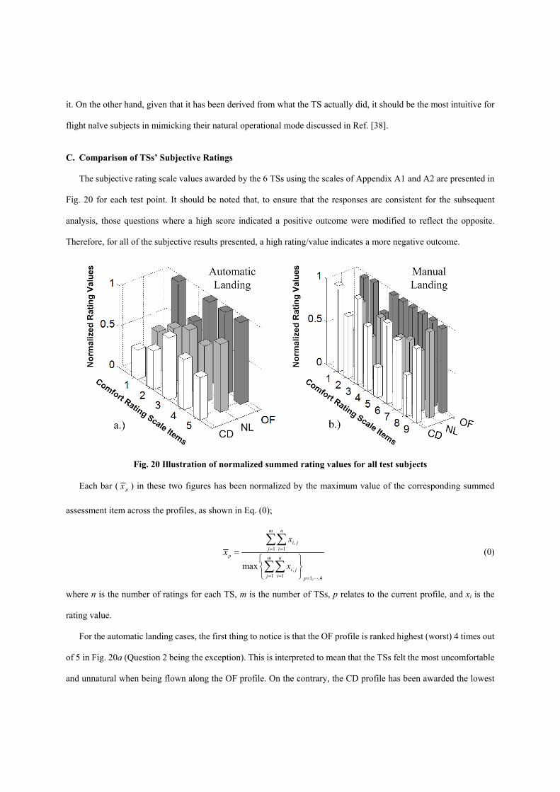
C. Comparison of TSs’ Subjective Ratings
The subjective rating scale values awarded by the 6 TSs using the scales of Appendix A1 and A2 are presented in
Fig. 20 for each test point. It should be noted that, to ensure that the responses are consistent for the subsequent
analysis, those questions where a high score indicated a positive outcome were modified to reflect the opposite.
Therefore, for all of the subjective results presented, a high rating/value indicates a more negative outcome.
Fig. 20 Illustration of normalized summed rating values for all test subjects
Each bar ( px ) in these two figures has been normalized by the maximum value of the corresponding summed
assessment item across the profiles, as shown in Eq. (0);
,1 1
,1 1 1, ,4
max
m n
i jj i
p m n
i jj i p
x
x
x
(0)
where n is the number of ratings for each TS, m is the number of TSs, p relates to the current profile, and xi is the
rating value.
For the automatic landing cases, the first thing to notice is that the OF profile is ranked highest (worst) 4 times out
of 5 in Fig. 20a (Question 2 being the exception). This is interpreted to mean that the TSs felt the most uncomfortable
and unnatural when being flown along the OF profile. On the contrary, the CD profile has been awarded the lowest

(best) rating 3 times (including Question 1- comfort level) out of the 5 possible. This suggests that the TSs felt at their
most comfortable during this maneuver. The rankings for the NL profile exist in between these two extremes but,
interestingly, it does achieve the best rating for feeling the most natural (Question 4).
The distribution of the ratings for the manual landing cases, shown in Fig. 20b, differs somewhat from the results
of the automatic landing. First, although the OF profile is still rated with the highest (worst) scores for 6 out of the 9
assessment items, the CD profile has been rated as the most uncomfortable maneuver overall by a small margin
(Question 1 in Appendix A2). Second, the NL profile has been rated the lowest (best) rating 5 times out of the 9
possible assessment items (including the key Questions 1 and 6 relating to the comfort level and how natural it felt,
respectively). This is interpreted to mean that the TSs generally felt at their most comfortable for this profile during
this form of the experiment.
Overall, these subjective results indicate that the OF is the least favorable profile among these three profiles for
both automatic and manual landing cases whilst the TSs preferred the CD profile for the automatic landing cases and
the designed NL profile for the manual landing cases, respectively.
D. Analysis of Control Effort
The root-mean-square (RMS) control inputs of the longitudinal and collective channels from the 6 TSs are
presented in Fig. 21. An individual case conducted by TS 1 has been plotted in Fig. 22 for illustrative purposes.
1 2 3 4 5 60.05
0.1
0.15
0.2
0.25
lon R
MS
,in
Test Subjects1 2 3 4 5 6
0.05
0.1
0.15
0.2
0.25
Test Subjects
col R
MS
,in
CD OF VL
Fig. 21 RMS values of control inputs (manual landing)

0 50 100 1500
0.1
0.2
0.3
0.4
0.5
lon,in
Time,sec0 50 100 150
-0.5
-0.4
-0.3
-0.2
-0.1
0
Time,sec
col,in
CD OF VL
Fig. 22 Illustration of control inputs of three profiles (TS 1)
The difference between the control inputs required for the three landing profiles in Fig. 21 is quite evident and
consistent with the results from the pilot model analysis. For the longitudinal input, the designed NL profile has input
amplitudes that are almost double the other two profiles. This is consistent with the theoretical analysis above. This
is due to the requirement to decelerate the PAV during the latter part of these two profiles, as depicted in Fig. 18 and
Fig. 22. For the CD profile, the TSs only need to move the stick to a fixed position and hold it there, as expected. For
the OF profile, the exponentially decreasing profile as well as the longest manoeuver period (170 sec) result in the
smallest RMS value. For the collective input, the three profiles have achieved generally similar levels of average
control input.
However, the control input information shown in Fig. 21 cannot provide any information about the TS’s level of
control aggressiveness, an effective measure of control workload, experienced during the manoeuver. This can be
addressed by calculating the control attack using Eq. (0). In this paper, one ‘attack’ is defined as being when a TS
makes a control input of more than 2% of full travel. The attack number per second (ANPS) can then be used to
describe the average number of control movements per second. The summed values of the ANPS, normalized by the
whole manoeuver period, are illustrated in Fig. 23.

12
3
12
34
56
0
5
10
Fig. 23 Mean attack number per second of longitudinal control input (manual landing)
The results in Fig. 23 emphasize the lowest control activity associated with the CD profile. Four of the 6 TSs
achieve the lowest ANPS for the CD approach during the three manual profiles flown. This is consistent with the
theoretical prediction in Fig. 18 and Fig. 19 i.e. that the TS only need to hold the stick due to the acceleration command
response type of the PAV system. The NL profile shows the largest attack number. This may be due to the aggressive
deceleration required (due to a smaller flight path angle when approaching the terminal phase of the maneuver, as
reflected in Fig. 19 and Fig. 22 ).
E. Assessment of Subjective Workload
The NASA Task Load Index (TLX) subjective workload assessment scale [39] was adopted for the qualitative
assessment of workload for the three landing profiles. The TLX rating scale was designed to be straightforward for
new test participants to understand the concepts involved in its use which was ideal for the flight-naïve TSs who had
no experience of using such rating scales. The TLX rating consists of an assessment of six aspects of workload –
mental demand; physical demand; temporal demand; performance; effort and frustration. A weighting system is then
used to combine the ratings for each of these aspects, in which the TS compares each workload element to all of the
other elements and decides in each case which represented the greater contribution to the overall workload of the task.
A final single workload score for each task is produced to represent the workload.
The average TLX ratings for each profile configuration given by the TSs who took part in the testing are shown in
Fig. 24. It can be seen that both the average TLX score and the TLX score standard deviation for each of the profiles

are very similar. Subjectively then, despite objective predictions and measures indicating that the NL profile might
generate the highest workload and the CD profile the lowest, the actual workload perceived by the test subjects did
not, on average, reflect this situation.
Fig. 24 Average TLX ratings from 6 TSs for three different landing profiles
F. Manual Flight Guidance-Following Precision
All three landing profiles for the manually-flown test cases were conducted by following the same form of
guidance symbology. Therefore, it might be expected that the profile for which the TSs achieved the smallest
deviations from the desired inputs might be considered to be the profile that is, in some way, ‘easiest’ to follow. The
forward speed and vertical position information are shown in Fig. 4. These parameters have been chosen for analysis
as they were the guidance signals used to drive the guidance symbology. The forward speed was not only used to drive
the commanded velocity but also to derive the acceleration command signal for the longitudinal cyclic. The vertical
position information was provided solely by the HITS. Therefore, the ability of a TS to successfully track a particular
profile is associated with the precision with which they adhere to these two parameters. The deviation errors for the
forward speed and vertical position, normalized by the maneuver period, are plotted in Fig. 25.
CD NL OF0
10
20
30
40
50
60
70
80
90
100
Landing Profile Configurations
Ave
rag
e T
LX
rat
ings

DCVL
OF
12
34
56
0
0.5
1
1.5
DCVL
OF
12
34
56
0
0.5
1
1.5
Fig. 25 Illustration of the normalized Vx and z-position deviation
The results in Fig. 25 show that the TS’s achieved the best task performance with the designed NL profile compared
with the other two tested profiles. For the Vx channel, Fig. 25a shows that all of the TSs exhibited the worst adherence
to the desired profile for the OF trajectory. However, 5 of the 6 TSs achieve the best precision for the NL profile. The
results for the vertical channel in Fig. 25b are similar, with the NL profile being the one that was followed most
accurately.
V. Discussion
The main thrust of the second-phase of the research was to answer the question as to which profile, amongst the
three profiles tested, was the most preferred by the TSs. This question is answered here by considering a number of
the issues of interest that arose during the above investigation. The rankings (1, 2, and 3 with 1 most favorable and 3
least favorable) of the three profiles with respect to the key features investigated above have been summarized in
Table 1 (automated landing) and Table 2 (manual landing).
Table 1 Comparisons of key features associated with three profiles (auto landing)
Profiles Discomfort Natural Feeling Sum
CD 1 2 3 OF 3 3 6
NL 2 1 3

Table 2 Comparisons of key features associated with three profiles (manual landing)
Profiles Discomfort Natural Feeling
Attack Number
Tracking Precision Sum
Vx z
CD 3 2 1 2 2 10 OF 2 3 2 3 3 13
NL 1 1 3 1 1 7
The results shown in the above two tables indicate that the answer to the research question is dependent upon the
point of interest. For example, the NL profile is ranked the highest based upon the subjective ratings for the manual
landing maneuver, but appears to require the highest control workload based upon the attack number. This trend in
workload is not reflected in the average subjective TLX scores awarded by the test subjects. This difference may have
arisen because of the different nature of the two measures. The attack number considers only the movement of the
control inceptor. However, the TLX rating asks the participants to consider a much broader range of parameters i.e.
not just the physical aspects but e.g. the mental loads being placed upon them. It appears from the results that, whilst
the stick activity did follow the model predictions, the other aspects of workload considered by the TLX rating scale
‘smoothed’ the overall perceived workload to be consistent across the profiles tested.
There are still a number of general comments that can be made based upon the results presented in these two
Tables. First, the OF profile was the least favored by the TSs. This profile is consistently ranked worst in Table 1 for
the automated landing cases and worst for 5 of the 7 factors in Table 2 for the manual landing. The poor rankings for
this profile are primarily due to the extended total period of the maneuver and the final sluggish approaching to the
Hover Board. TS comments indicated that this resulted in the approach feeling unnatural and uncomfortable and that
they became increasingly irritated the longer that it progressed. The same issue was also reported in Ref. [40] in which
the author proposed a hybrid profile – the initial OF stage followed by the CD to overcome the problem for professional
pilots. Second, the preference for a profile is dependent upon the mode of operation i.e. automated or manual. For the
automatic landing, the CD profile is the most preferred. It is ranked as being lowest in terms of discomfort and felt the
most natural to the participants. However, for the manual landing, the NL profile was the overall preferred option. It
was rated as providing the most general subjective comfort and having the most natural-feel by the TS. If the
requirement is to achieve the highest tracking performance and the trajectory that PAV occupants feel is the most
natural, then the NL profile would be the profile of choice for a manually flown descent.

VI. Conclusions
The aim of the study reported in this paper was to ascertain what kind of landing approach trajectory would be
most suited to flight-naïve occupants of a personal aerial vehicle for both manual and automated flight. A trajectory
was developed based upon simulated flight data obtained using flight-naïve test subjects. This ‘natural landing’ (NL)
trajectory was then compared with two other approach types that have been reported in the literature: constant
deceleration (CD) and constant optical flow (OF). Based upon the results of this study, the following conclusions can
be drawn:
Somewhat unexpectedly, the longitudinal trajectory selected by the flight-naïve participants could be modelled
by an idealized approach profile previously obtained for professional helicopter pilots.
The final stages of the approach to hover could be modeled using Tau theory and specifically by coupling the
taus of height and longitudinal distance to the hover point.
Despite potentially offering the safest approach in terms of low terminal velocity and being the method taught
to trainee helicopter pilots, the participants’ least preferred approach profile was constant optical flow for both
manual and automated approaches.
Whilst subjective methods of workload assessment were met the predictions made by observing the output of
a pilot model, the subjective measure of workload used indicated broad agreement in perceived workload across
the three profiles tested.
For the automated approach task used, the participants preferred the constant deceleration profile used.
Despite theoretical analysis indicating that it might pose some workload and skill issues for flight-naïve pilots,
for a manually flown approach, the participants preferred the natural landing profile, designed for this study,
based upon a number of indicators used.
Appendix
A1. Comfort Rating Scale for Automatic Landing
The highlighted terms in green have a positive meaning for the higher scores. For the other items, a high score has a
negative connotation.

A2. Comfort Rating Scale for Manual Landing
The highlighted terms in green have the positive meaning.

Acknowledgments
The work reported in this paper is funded by the EC FP7 research funding mechanism under grant agreement no.
266470. The authors would like to thank all those who have participated in the simulation trials reported in this paper
for their contributions to the research. Mr. Max Aldridge and Ms. Natalia Cooper in the Faculty of Psychology, Health
and Society at the University of Liverpool is acknowledged for their help in designing the subjective rating scales
used in this work.
References
[1] Uhlemann, E., "Autonomous Vehicles Are Connecting...," Vehicular Technology Magazine, IEEE, published
online 2015; Vol. 10, No. 2, pp. 22-25. Doi: 10.1109/MVT.2015.2414814.
[2] Le Vine, S., Zolfaghari, A., and Polak, J., "Autonomous Cars: The Tension between Occupant Experience and
Intersection Capacity," Transportation Research Part C: Emerging Technologies, published online Mar.2015;
Vol. 52, pp. 1-14, DOI: 10.1016/j.trc.2015.01.002
[3] Wagner, S., “Autonomous Cars Could Let Drivers Check Email," Engineer, published online July 2015; Vol. 12,
pp. 1-3.
[4] Anon., “ICAO Cir 328, Unmanned Aircraft System (UAS)", 978-92-9231-751-5, 2011
[5] Roux. Y., "OPTIMAL Final Publishable Report," WP0-AIF-310-V1.1-ED-PU, Airbus France, Dec.2008.
[6] Lawrence, B., and Padfield, G. D., "Wake Vortex Encounter Severity for Rotorcraft in Approach and Landing,"
Proceedings of the 31st European Rotorcraft Forum, Florence, Italy, 2005, pp. 1-16.
[7] Jump, M., Perfect, P., Padfield, G.D., "myCopter: Enabling technologies for personal transportation systems. An
early progress report," Proceedings of the 37th European Rotorcraft Forum, Vol. 1, Curran Associates Inc., Red
Hook, NY, 2011, pp. 336-347.
[8] Heffley, R.K., “A Model for Manual Decelerating Approaches to Hover", Proceedings of the 15th Annual
Conference on Manual Control, AFFDL-TR-79-3134, pp. 545-554, Dayton, Ohio, March 20 - 22, 1979.
[9] Lockett, H. A., "The Role of Tau-Guidance during Declarative Helicopter Approaches," Faculty of Engineering,
University of Liverpool, Liverpool, 2010.
[10] Moen, G. C., DiCarlo, D. J., Yenni, K. R., “A Parametric Analysis of Visual Approaches for Helicopters,” NASA-
TN-D-8275, L-10841, Washington, United States, 1976.

[11] Neiswander, G. M., "Improving Deceleration Guidance for Rotorcraft Brownout Landing," Master Thesis,
University of Iowa, 2010, 2010.
[12] Perrone, J. A., "The Perception of Surface Layout during Low Level Flight," NASA CP 3118, 1991.
[13] Phatak, A. V., Jr. Peach, L. L., Hess, R. A., Ross, V. L., Hall, G. W., and Gerdes, R. M., "A Piloted Simulator
Investigation of Helicopter Precision Decelerating Approaches to Hover to Determine Single-Pilot IFR /SPIFR/
Requirements," Guidance and Control Conference, AIAA PAPER 79-1886, Boulder, CO, August 6-8, 1979.
[14] White, M., Perfect, P., Padfield, G.D., "Acceptance Testing and Commissioning of A Flight Simulator for
Rotorcraft Simulation Fidelity Research," Proceedings of the Institution of Mechanical Engineers, Part G: Journal
of Aerospace Engineering, Vol. 227, No. 4, 2012, pp. 663-686. Doi: 10.1177/0954410012439816.
[15] Padfield, G. D., Helicopter Flight Dynamics, 2nd ed., Blackwell Science, Oxford, 2007.
[16] Srinivasan, M. V., Zhang, S. W., Chahl, J. S., Chahl, J. S., and Venkatesh, S., " How Honeybees Make Grazing
Landings on Flat Surfaces," Biol Cybern, published online 2000; Vol. 80, No. 3, pp. 172-183.
[17] Izzo, D., Weiss, N., and Seidl, T., “Constant-Optic-Flow Lunar Landing: Optimality and Guidance,” Journal of
Guidance, Control, and Dynamics, published online Sept. 2011; Vol. 34, No. 5, pp. 1383-1395. DOI:
10.2514/1.52553.
[18] Green, W., and Oh, P., "Optic Flow Based Collision Avoidance on a Hybrid MAV," IEEE Robotics and
Automation Magazine, Vol. 15, No. 1, pp. 96–103, 2008. Doi:10.1.1.122.600.
[19] Franceschini, N., Ruffier, F., Serres, J., and Viollet, S., “Optic Flow Based Visual Guidance: From Flying Insects
to Miniature Aerial Vehicles”, edited by. T. M. Lam, in Aerial Vehicles, 2009, pp. 747-770.
[20] Szoboszlay, Z., Albery, W. B., Turpin, T., and Neiswander, G. M., "Brown-Out Symbology Simulation (BOSS)
on the NASA Ames Vertical Motion Simulator," American Helicopter Society 64th Annual Forum, Montreal,
Quebec, Canada, 29th April - 1st May 2008
[21] Anon., “Handling Qualities Requirements for Military Rotorcraft US Army Aviation and Missile Command”,
ADS-33E-PRF, 2000.
[22] Lee, D. N., “Guiding Movement by Coupling Taus,” Ecological Psychology, published online 1998; Vol. 10, No.
3, pp. 221-250. Doi:10.1207/s15326969eco103&4_4.
[23] Lee, D. N., Craig, C. M., and Grealy, M. A., “Sensory and Intrinsic Coordination of Movement,” Proceedings of
Biological sciences, published online Jul. 1999; Vol. 266, No. 1432, pp. 2029-2035. Doi: 10.1098/rspb.1999.0882

[24] Lee, D. N., “Tau in Action in Development,” Action as an Organizer of Learning and Development, edited by.
J. J. Rieser, J. J. Lockman, and C. A. Nelson, 33rd Volume in the Minnesota Symposium on Child Psychology,
Minnesota, 2005, pp. 3-50.
[25] Padfield, G. D., “The Tau of Flight Control,” Aeronautical Journal, published online Sept. 2011; Vol. 115, No.
1171, pp. 521-555.
[26].Clark, G., “Helicopter Handling Qualities in Degraded Visual Environments,” PhD Thesis, Department of
Engineering, The University of Liverpool, UK, 2007.
[27] Padfield, G. D., Lee, D. N., and Bradley, R., “How Do Helicopter Pilots Know When to Stop, Turn or Pull Up?,”
Journal of the American Helicopter Society, published online 2003; Vol. 48, No. 2, pp. 108-119. Doi:
10.4050/JAHS.48.108.
[28] Padfield, G. D., Clark, G., and Taghizad, A., “How Long Do Pilots Look Forward? Prospective Visual Guidance
in Terrain-Hugging Flight,” Journal of the American Helicopter Society, Vol. 52, No. 2, 2007, pp. 134-145. Doi:
10.4050/JAHS.52.134.
[29] Jump, M., and Padfield, G. D., “Investigation of the Flare Maneuver Using Optical Tau,” Journal of Guidance,
Control, and Dynamics, published online Sept. 2006; Vol. 29, No. 5, pp. 1189-1200. Doi: 10.2514/1.20012
[30] Lee, D. N., “A Theory of Visual Control of Braking Based on Information about Time-To-Collision,” Perception,
published online 1976; Vol. 5, No. 4, pp. 437-459. Doi:10.1068/p050437.
[31] Meyer, M., and Padfield, G. D., “First Steps in the Development of Handling Qualities Criteria for a Civil Tilt
Rotor,” Journal of the American Helicopter Society, published online Jan. 2005, Vol. 50, No. 1, pp.33-46. Doi:
10.4050/1.3092841
[32] Lu, L., Jump, M., and Jones, J., “Tau Coupling Investigation Using Positive Wavelet Analysis,” Journal of
Guidance, Control, and Dynamics, published online 2013, Vol. 36, No. 4, pp. 920-934. Doi: 10.2514/1.60015.
[33] Perfect, P., White, M., Padfield, G. D., and Gubbels, A. W., "Rotorcraft Simulation Fidelity: New Methods for
Quantification and Assessment," The Aeronautical Journal, Vol. 117, No. 1189, pp. 235-282, Mar.2013.
[34] Perfect, P., White, M. D., and Jump, M., “Methods to Assess the Handling Qualities Requirements for Personal
Aerial Vehicles,” Journal of Guidance, Control, and Dynamics, accepted for publication, 2015. Doi:
10.2514/1.G000862

[35] Malcolm, R., “The Malcolm Horizon—History and Future,” NASA Conference Publication 2306: Peripheral
Vision Horizon Display, NASA, Edwards, CA, 1983, pp. 11–40
[36] Nolan-Proxmire, D., and Henry, D., “Highway in the Sky Ready for Atlanta Olympics”, NO. 96-071, NASA
Langley Research Center, Hampton, VA, July 1996.
[37] McRuer, D. T., and Krendel, E. S., “Mathematical Models of Human Pilot Behavior,” AGARD-AG-188,
Jan.1974.
[38] McRuer, D. T., "Pilot-Induced Oscillations and Human Dynamic Behavior," NASA Contractor Report 4683,
Jul.1995.
[39] Lu, L., Jump, M., Perfect, P., and White, M. D., "Development of a Visual Landing Profile with Natural-Feeling
Cues," Proc. American Helicopter Society 70th Annual Forum, Montreal, Quebec, Canada, 20th-21st, May 2014.
[39] Hart, S. G. and Staveland, L. E., Development of NASA-TLX (Task Load Index): Results of Empirical and
Theoretical Research, In Hancock, P. A., and Meshkati, N. (Eds.), Human Mental Workload. Amsterdam: North
Holland Press, 1988.