Arterial stents: modelling drug release and restenosis

J.E.F. Green1, G.W. Jones2, L.R. Band1 and A. Grief1

1Centre for Mathematical Medicine, School of Mathematical Sciences,University of Nottingham, Nottingham, NG7 2RD, UK.

2 OCIAM, Mathematical Institute, University of Oxford, Oxford, UK.

1 Biological background

An arterial stent is a contemporary medical device used to prevent ischemia (inadequate bloodflow) caused by the growth of an atherosclerotic plaque inside an artery wall.

Artery walls have three layers. The inner layer is the intima; this contains the endothelium,a layer of cells directly next to the blood which play an important role in controlling vasculartone, regulating transport into the wall and inhibiting smooth muscle cell proliferation andmigration (Corti and Badimon, 2002). The middle layer is the media which is the muscularpart of the wall, containing smooth muscle cells, collagen and elastin. The outer layer is theadventitia which contains fibrous tissue (making it much stiffer than the media) and tethersthe artery to the perivascular tissue.

When atherosclerosis occurs, a plaque consisting of lipid and fibrous tissue forms inside theintima layer of the artery wall (Libby, 2000; Yuan et al., 2000). Atherosclerosis is the mostcommon arterial disease and can lead to heart attacks and strokes, making it the leading causeof death in the Western world. As the plaque grows the artery wall thickens; a large plaque maygreatly reduce the lumenal area, reducing the blood flow and resulting in insufficient oxygenbeing obtained by the tissues downstream (ischemia).

One clinical procedure to increase or maintain the lumen is percutaneous translumenal coro-nary angioplasty (PTCA) where a wire object called a stent, shown in Figure 1(a), is placedinside the vessel to provide an internal scaffold to hold the walls apart. The wire stent ismounted on to a balloon catheter, Figure 1(b). During surgery the catheter is used to manoeu-vre the stent along the blood vessels, to the diseased artery. Once the stent has been positionedat the site of the atherosclerotic plaque the balloon is inflated, causing the stent to expand indiameter and push the artery walls apart, as illustrated in Figure 1(c). The balloon is thenremoved, leaving the stent in situ as a permanent implant, increasing the area of the lumen,Figure 1(d). By relieving the blockage of the artery in this manner blood flow and oxygentransport to the tissues downstream are improved, reducing the likelihood that the patient willsuffer from a heart attack or stroke.

The insertion of a stent causes some damage to the vessel and often the endothelium is re-moved during the process and the stent contacts the smooth muscle cells of the artery’s medialayer. Until the endothelium grows back, over a period of about four weeks, the endothelium’sability to inhibit smooth muscle cell proliferation is lost and the vessel wall may thicken over

1

Report on a problem studied at the UK Mathematics-in-Medicine Study Group Strathclyde 2004< http://www.maths-in-medicine.org/uk/2004/arterial-stents/ >

the stent and reduce the lumenal area, a process called restenosis. The stent provokes aninflammatory response, which causes factors to be released which could also encourage tissuegrowth and restenosis. The high incidence of restenosis is a huge disadvantage of this clinicaltechnique and often an atherosclerotic vessel must be stented several times before a suitablywide lumen is obtained.

To reduce restenosis after PTCA drugs such as paclitaxel and rapamycin can be mixed witha polymer and coated on to the stent (Alexis et al., 2004). These drugs diffuse into the arterywall where they are taken up by the smooth muscle cells. The drugs interrupt their cell cycleand thus prevent their proliferation. This is a recent technique however and we lack knowledgeof which factors affect its success. Clinicians would like to obtain a uniform drug distributionover the arterial wall, however the arterial wall morphology, stent design and physiochemicalproperties of the drug are likely to affect the drug distribution obtained by the cells (Sousaet al., 2003). By mathematically modelling the drug transport across the artery wall, the sub-sequent uptake by the cells, and the effect of this upon the tissue growth, we hope to gaininsight into the effectiveness of drug coated stents in preventing restenosis.

2 Review of mathematical models

In modelling the release of drug from arterial stents, and its impact on restenosis, a number ofissues must be considered. A comprehensive modelling treatment would aim to couple haemo-dynamics, cell proliferation and drug diffusion through both the stent’s polymer coating andthe different layers of the artery wall. At present, such a complete treatment is still some wayoff. However, some insights have been gained through mathematical modelling of particularaspects of the problem. The aim of this section is to describe the main modelling issues, anddiscuss a few of the published models which have attempted to tackle them.

Drug transport across the artery wall occurs both by diffusion and convection with the bloodplasma. From a fluid dynamic point of view, the artery wall may be treated as a porous medium,and hence the radial flow can be modelled using Darcy’s law (Zunino, 2004). The anisotropicnature of the wall material means that the rate of diffusion of the drug may be different indifferent directions; for one particular type of drug, the planar and transmural diffusivitieswere found to differ by a factor of 45 (Hwang and Edelman, 2002). It may also be necessaryto distinguish between solution (plasma) drug concentration and tissue drug concentration, asthe hydrophobicity of some drugs may lead to preferential accumulation within the tissue. Thiseffect is modelled by introducing a partition coefficient K, such that in steady state the cellulartissue drug concentration cT is given by:

cT = KcE, (1)

where cE is the drug concentration in the extracellular fluid. In general, K may be concentra-tion, space and time dependent (Hwang et al., 2003). Multi-region models may be employed totake account of the different drug transport properties of different regions of the arterial wall,and within the stent coating (Zunino, 2004).

2

(a)

(b)

(c)

(d)

Figure 1: (a) A sketch of a wire mesh stent. (b) The tip of a balloon catheter, with a stentin compressed form mounted on the balloon. (c) A sketch showing the balloon catheter withstent in position at the site of an atherosclerotic plaque. Plaques cause a localised narrowingof the vessel which restricts blood flow. The arrows indicate direction of the expansion of theballoon. (d) The stent, after balloon inflation and catheter withdrawal. The stent holds openthe lumen of the artery.

3

Clinically, several different designs of stent are used for implantation into patients. Thestents are generally constructed of a wire mesh; however, the design of the mesh varies betweenstents. These design differences can affect the haemodynamics close to the artery wall, andlead to regions of unusually low or high wall shear stress (WSS). Low WSS is correlated withthrombus formation, whilst high stress may damage blood cells and cause platelet activation. InMontagano et al. (2003), computational fluid dynamics is applied to studying the distributionof WSS for two particular stent designs, and the implications for the likelihood of restenosis.Their conclusions appear to agree with clinical data, which show a difference of about 4% inrestenosis rates between the two designs.

3 Modelling drug release from an arterial stent

3.1 Material properties

The wires forming the stent are assumed to be cylindrical with radius rwire = 5 × 10−5 m, andcoated with polymer to a thickness of h = 10−5 m. The drug is embedded in the polymer andis released by a diffusion process, assumed to be isotropic. The diffusivity of the drug withinthe stent coating, DP , is dependent on the polymer used, but values cited in the literature arearound 10−14 m2 s−1, with some reported values as low as 10−16 m2 s−1.

The drug will diffuse through the media, which has a thickness of around d = 4 × 10−4 mand a porosity of φ = 0.61. The diffusion is noticeably anisotropic, with diffusivities in thelongitudinal and circumferential directions of the order of 10−10 m2 s−1, while the diffusivity inthe radial direction is of the order of 10−12 m2 s−1 or less. We also note that there is a fluidflow from the blood vessel lumen to the cells due to the difference between the arterial bloodpressure and the fluid pressure in the surrounding tissues. This fluid flow has been measuredto have a discharge (volume flux per unit area) of around v = 10−8 m s−1.

One of the most popular drugs used to prevent restenosis is paclitaxel. The tissue bindingproperties of this drug are described by Levin et al. (2004), who conducted an experimentwhere specimens of artery tissue are placed in a bath containing a solution of paclitaxel atconcentration c. The tissue is left in the solution for a period of 60 hours, after which it isremoved and analysed. The final concentration of drug in the artery wall tissue, cfinal

T is foundon average to be 30 times the concentration c. A more detailed analysis showed that the bindingcapacity K, defined to be the ratio of drug concentration at any point in the tissue to c, variesfrom a range of 13–25 in the media to around 16–45 in the adventitia. In this report we willassume a representative value for the media of K = 15, such that

cfinalT = K c, where K = 15. (2)

A separate experiment cited in Levin et al. (2004) measures the concentration of drug inarterial samples placed in a bath of paclitaxel solution over a period of 72 hours. The drugconcentration in the tissue sample, cT(t), is measured at regular intervals. The results comparedto the final equilibrium value, cfinal

T , obtained at 72 hours following a 12-hour steady-state period.The evolution of cT can be described by a first order reaction kinetics model, in which the rate

4

of change of cT is proportional to the distance from the equilibrium value,

d cT

dt= α

(cfinalT − cT

). (3)

Equation 3, subject to the initial condition cT(0) = 0, can be solved to show

cT(t) = cfinalT

(1 − e−αt

). (4)

Comparison of this model with the experimental data presented in Levin et al. (2004) showsgood agreement. The rate constant α is found to be around 2 × 10−5 s−1.

3.2 Drug delivery model

Any attempt at modelling a problem of this kind will require an understanding of the diffusionof drug from the polymer-coated stent through to the blood vessel wall. We will thereforeconsider at first only this aspect of the problem, neglecting the smooth muscle cell prolifera-tion. This simplification of the model is valid if the timescale for the drug transport is shortcompared with the timescale for muscle cell growth, which can be shown to be a reasonableassumption using experimental data.

The complicated physiology of the artery wall will be simplified to the geometry portrayedin Figure 2. We will only consider two domains through which the drug is assumed to diffuse,namely the polymer coating the wire, and the smooth muscle cells that comprise the media.

We suppose that the concentration of the drug in the polymer is denoted cP . The transportof drug within the polymer is assumed to be dominated by diffusion, so that:

∂cP

∂t= DP

(∂2cP

∂x2+

∂2cP

∂y2

)(5)

in the polymer, where DP is the diffusivity of the drug in the polymer.

We consider the media as a porous medium consisting of a cell phase and the extracellularfluid. We denote the concentration in the two phases by cI (the cell phase) and by cE (extra-cellular fluid). Drug transport through the extracellular fluid is assumed to occur through bothconvection (due to the fluid flow from the blood through the media, with discharge u = −vj)and (anisotropic) diffusion. We also assume that the drug is absorbed by the cells at a rateQ(cE , cI), and that once the drug is attached to a cell, it does not diffuse through the cell. Inthe media, we therefore have:

φ∂cE

∂t− v

∂cE

∂y= Dx

∂2cE

∂x2+ Dy

∂2cE

∂y2− Q (6)

(1 − φ)∂cI

∂t= Q (7)

where φ is the porosity of the medium. Note that we have supposed that the velocity field isconstant and unaffected by the presence of the stent, which is physically unrealistic but avoids

5

Adventitia

Wire

Polymer

Media

Blood

Figure 2: Simplified geometry of the two-dimensional model

the necessity of solving a fluid flow problem in the domain.

We choose:

Q = α(cE − cI

K

)(8)

so that the rate at which the cells absorb the drug is proportional to the extracellular con-centration initially, but that the ratio of internal concentration to extracellular concentrationequilibrates to K.

The boundary conditions for the problem are, on the whole, intuitive. At the boundarybetween the polymer and the wire, we require zero flux of the drug into the impermeable metalwire. Where the polymer is in contact with the blood, any amount of drug reaching the blood-stream will be washed away by the relatively fast flowing blood. Therefore the concentrationat the blood-polymer interface will be very low, and we impose the boundary condition cP = 0at this boundary. Similar considerations lead us to prescribe cE = 0 at the boundary where themedia is in contact with the blood. At the interface of the media and the polymer we imposecontinuity of extracellular drug concentration and polymer drug concentration, and also conti-nuity of the corresponding fluxes of the drug. Accounting for both the adjective and diffusive

6

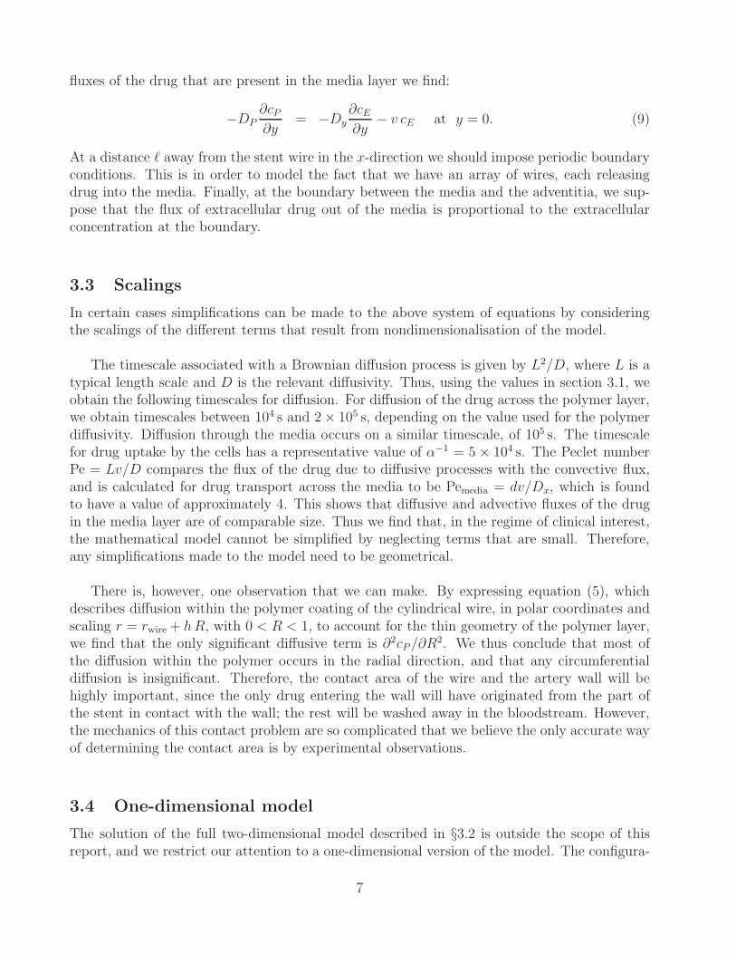
fluxes of the drug that are present in the media layer we find:

−DP∂cP

∂y= −Dy

∂cE

∂y− v cE at y = 0. (9)

At a distance � away from the stent wire in the x-direction we should impose periodic boundaryconditions. This is in order to model the fact that we have an array of wires, each releasingdrug into the media. Finally, at the boundary between the media and the adventitia, we sup-pose that the flux of extracellular drug out of the media is proportional to the extracellularconcentration at the boundary.

3.3 Scalings

In certain cases simplifications can be made to the above system of equations by consideringthe scalings of the different terms that result from nondimensionalisation of the model.

The timescale associated with a Brownian diffusion process is given by L2/D, where L is atypical length scale and D is the relevant diffusivity. Thus, using the values in section 3.1, weobtain the following timescales for diffusion. For diffusion of the drug across the polymer layer,we obtain timescales between 104 s and 2× 105 s, depending on the value used for the polymerdiffusivity. Diffusion through the media occurs on a similar timescale, of 105 s. The timescalefor drug uptake by the cells has a representative value of α−1 = 5 × 104 s. The Peclet numberPe = Lv/D compares the flux of the drug due to diffusive processes with the convective flux,and is calculated for drug transport across the media to be Pemedia = dv/Dx, which is foundto have a value of approximately 4. This shows that diffusive and advective fluxes of the drugin the media layer are of comparable size. Thus we find that, in the regime of clinical interest,the mathematical model cannot be simplified by neglecting terms that are small. Therefore,any simplifications made to the model need to be geometrical.

There is, however, one observation that we can make. By expressing equation (5), whichdescribes diffusion within the polymer coating of the cylindrical wire, in polar coordinates andscaling r = rwire + h R, with 0 < R < 1, to account for the thin geometry of the polymer layer,we find that the only significant diffusive term is ∂2cP /∂R2. We thus conclude that most ofthe diffusion within the polymer occurs in the radial direction, and that any circumferentialdiffusion is insignificant. Therefore, the contact area of the wire and the artery wall will behighly important, since the only drug entering the wall will have originated from the part ofthe stent in contact with the wall; the rest will be washed away in the bloodstream. However,the mechanics of this contact problem are so complicated that we believe the only accurate wayof determining the contact area is by experimental observations.

3.4 One-dimensional model

The solution of the full two-dimensional model described in §3.2 is outside the scope of thisreport, and we restrict our attention to a one-dimensional version of the model. The configura-

7

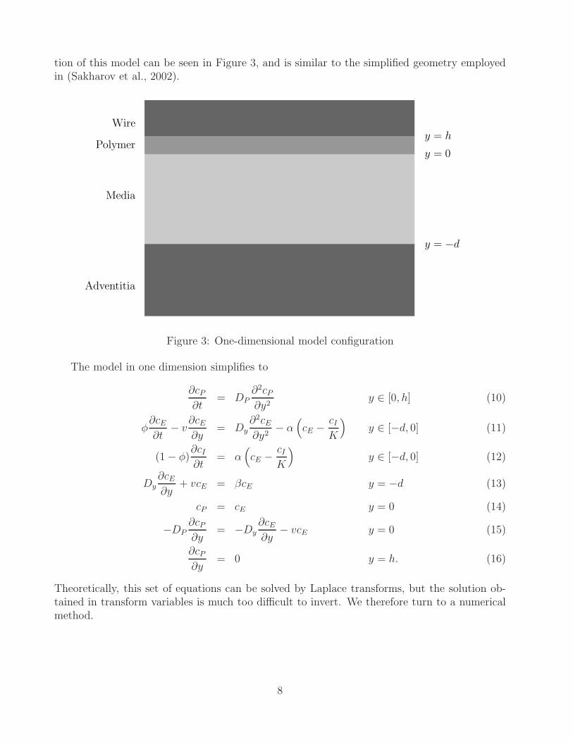
tion of this model can be seen in Figure 3, and is similar to the simplified geometry employedin (Sakharov et al., 2002).

Adventitia

Media

Polymer

Wire

y = −d

y = 0

y = h

Figure 3: One-dimensional model configuration

The model in one dimension simplifies to

∂cP

∂t= DP

∂2cP

∂y2y ∈ [0, h] (10)

φ∂cE

∂t− v

∂cE

∂y= Dy

∂2cE

∂y2− α

(cE − cI

K

)y ∈ [−d, 0] (11)

(1 − φ)∂cI

∂t= α

(cE − cI

K

)y ∈ [−d, 0] (12)

Dy∂cE

∂y+ vcE = βcE y = −d (13)

cP = cE y = 0 (14)

−DP∂cP

∂y= −Dy

∂cE

∂y− vcE y = 0 (15)

∂cP

∂y= 0 y = h. (16)

Theoretically, this set of equations can be solved by Laplace transforms, but the solution ob-tained in transform variables is much too difficult to invert. We therefore turn to a numericalmethod.

8

3.5 Numerical simulations

The one-dimensional model described in §3.4 was solved numerically using a simple finite differ-ence scheme, implemented in Matlab. A numerically stable scheme for this advection-diffusionsystem was obtained using the fully-implicit backward Euler time-stepping method.

In the absence of data for the value of the parameter β, which occurs in the boundarycondition (13) at the bottom of the media layer, y = −d, three cases were considered. Twolimiting cases were examined in which the flux of the drug out of the media layer was (i) veryslow, modelled by choosing β = 0, and (ii) very rapid, for which we consider the limit β → ∞.A third value, β = Dy/d was chosen to represent an intermediate case, in which the flux outof the media layer is comparable in magnitude with the diffusive fluxes present within the media.

Profiles of cP , cE and cI , at regular time intervals between t = 0 s and t = 105 s, areshown in Figure 4. The model is linear with respect to the concentrations, cE , cI and cP ,thus the results scale linearly with the initial drug concentration in the polymer. Therefore allconcentrations are normalised by the initial drug concentration in the polymer at time t = 0 s,and all plots show the normalised concentration values. Profiles are shown for the three valuesof β discussed above and two values of α, the cellular drug uptake rate constant: the first value,α = 2× 10−5 s−1, is derived from data in Levin et al. (2004) as described in §3.1, and a secondset of results, which represent a more reactive drug with α = 2× 10−4 s−1, are also shown. Theother parameter values are the same as in §3.1:

DP = 1.0 × 10−14 m2 s−1, Dy = 1.0 × 10−12 m2 s−1, h = 1.0 × 10−5 m,

d = 4.0 × 10−4 m, v = 1.0 × 10−8 m s−1, K = 15, φ = 0.61.

Figure 5 shows the time variation of the mass of drug within the polymer, extracellular fluidand the cells of the media layer. E.g. at time t = 0, all the drug is contained within thepolymer, and none is present within the extracellular fluid or the cells. The total mass of thedrug within the system is also shown. For β �= 0, the total mass decreases with time as massis lost to the lower layers of the artery wall.

We see in Figure 4 and 5 that the drug escapes rapidly from the polymer layer. The resultsshow that a more reactive drug (with α = 2 × 10−4) is initially better absorbed by the cellsof the medial layer than the drug with lower reactivity. The fast absorption of the drug bythe cells initially prevents the more reactive drug from being washed out of the system by theadvective flux. This is shown by the absence in Figures 5(d),(f) of the rapid decrease in thetotal drug mass within the system by time t = 0.5 days which is clearly visible in figures 5(c),(e).

At longer times, t > 2.5 days, it appears that the cellular drug concentration is moststrongly effected by β, which regulates the flux of the drug leaving the system. This is becauseour model describes reversible binding of the drug to the cells. Thus for large β, for which theextracellular drug is easily removed from the system, the low levels of cE cause the drug tounbind from the cells more rapidly.

9

The concentration of the drug in cells near the surface of the media layer, y = 0, maybe of clinical interest, as these cells may play a significant role in vessel restenosis. The timevariation of this quantity is shown in Figure 6. We see that increasing the drug activity, α,leads to a considerable increase in the amount of drug absorbed at y = 0. The results for theconcentration cI at the surface y = 0 are found to be almost independent of the flux parameterβ.

4 Modelling restenosis

In this section, we shall investigate models for the proliferation of smooth muscle cells (SMC)in a stented artery, and the resulting restenosis of the vessel.

4.1 Model formulation - tissue growth

We assume the artery is an axisymmetric tube, of which we consider a two-dimensional cross-section. The lumen of the vessel is assumed to have radius a(t), whilst the radius of the vesselup to the media / adventitia interface is R∗ (taken as constant). As a simplification, we shalltreat the stent as a hoop, of radius Rs. We shall now develop a model for the proliferation of thesmooth muscle cells in the artery wall, based on the tumour growth model of Franks and King(Franks and King, 2003; King and Franks, 2004). We let n be the volume fraction of SMCswithin the intima, and ρ is taken to be the volume fraction of cellular debris and extracellularfluid. We assume there are no voids, so that:

n + ρ = 1. (17)

We let the concentration of drug be c (equations describing its transport within the layer ofproliferating cells will be derived in §4.2). Both cells and cellular debris / fluid are assumedto move with the same velocity v; cells proliferate at a rate g(n, c) and die at a rate f(n, c),whence they become part of the cellular debris phase. Cellular debris is removed, e.g. by theimmune system, at a rate h(n, c). Our governing equations are then:

∂n

∂t+ ∇ · (nv) = g(n, c) − f(n, c), (18)

∂ρ

∂t+ ∇ · (ρv) = f(n, c) − h(n, c). (19)

We note that, by adding the two equations above, we obtain:

∇ · v = g − h. (20)

In general, this equation would require a constitutive relation to close the system (e.g. Darcy’slaw, or Stokes’ law); however, this is not necessary in the one-dimensional case which follows.

4.1.1 Drug-free case: uniform proliferation

We restrict our attention to the one-dimensional axisymmetric case, and assume that the volumefraction of cells (and hence cellular debris) remains constant within the artery wall. We take the

10

(a) β = 0 ms−1, α = 2 × 10−5s−1 (b) β = 0 ms−1, α = 2 × 10−4s−1

−4 −3 −2 −1 0

x 10−4

0

0.05

0.1

y, on range [−d,0]Ext

race

llula

r C

once

ntra

tion,

cE 0 0.1 0.2 0.3 0.4 0.5 0.6 0.7 0.8 0.9 1

x 10−5

0

0.5

1

y, on range [0,h]

Pol

ymer

Con

cent

ratio

n, c

P

−4 −3 −2 −1 0

x 10−4

0

0.05

0.1

0.15

0.2

y, on range [−d,0]

Cel

lula

r C

once

ntra

tion,

cI

−4 −3 −2 −1 0

x 10−4

0

5

10x 10

−3

y, on range [−d,0]Ext

race

llula

r C

once

ntra

tion,

cE 0 0.1 0.2 0.3 0.4 0.5 0.6 0.7 0.8 0.9 1

x 10−5

0

0.5

1

y, on range [0,h]

Pol

ymer

Con

cent

ratio

n, c

P

−4 −3 −2 −1 0

x 10−4

0

0.05

0.1

0.15

0.2

y, on range [−d,0]

Cel

lula

r C

once

ntra

tion,

cI

(c) β = 2.5 × 10−9 ms−1, α = 2 × 10−5s−1 (d) β = 2.5 × 10−9 ms−1, α = 2 × 10−4s−1

−4 −3 −2 −1 0

x 10−4

0

0.02

0.04

0.06

y, on range [−d,0]Ext

race

llula

r C

once

ntra

tion,

cE 0 0.1 0.2 0.3 0.4 0.5 0.6 0.7 0.8 0.9 1

x 10−5

0

0.5

1

y, on range [0,h]

Pol

ymer

Con

cent

ratio

n, c

P

−4 −3 −2 −1 0

x 10−4

0

0.02

0.04

0.06

0.08

y, on range [−d,0]

Cel

lula

r C

once

ntra

tion,

cI

−4 −3 −2 −1 0

x 10−4

0

2

4

6x 10

−3

y, on range [−d,0]Ext

race

llula

r C

once

ntra

tion,

cE 0 0.1 0.2 0.3 0.4 0.5 0.6 0.7 0.8 0.9 1

x 10−5

0

0.5

1

y, on range [0,h]

Pol

ymer

Con

cent

ratio

n, c

P

−4 −3 −2 −1 0

x 10−4

0

0.05

0.1

0.15

0.2

y, on range [−d,0]

Cel

lula

r C

once

ntra

tion,

cI

(e) β → ∞, α = 2 × 10−5s−1 (f) β → ∞, α = 2 × 10−4s−1

−4 −3 −2 −1 0

x 10−4

0

5

10

15x 10

−3

y, on range [−d,0]Ext

race

llula

r C

once

ntra

tion,

cE 0 0.1 0.2 0.3 0.4 0.5 0.6 0.7 0.8 0.9 1

x 10−5

0

0.5

1

y, on range [0,h]

Pol

ymer

Con

cent

ratio

n, c

P

−4 −3 −2 −1 0

x 10−4

0

0.01

0.02

0.03

0.04

y, on range [−d,0]

Cel

lula

r C

once

ntra

tion,

cI

−4 −3 −2 −1 0

x 10−4

0

2

4

6x 10

−3

y, on range [−d,0]Ext

race

llula

r C

once

ntra

tion,

cE 0 0.1 0.2 0.3 0.4 0.5 0.6 0.7 0.8 0.9 1

x 10−5

0

0.5

1

y, on range [0,h]

Pol

ymer

Con

cent

ratio

n, c

P

−4 −3 −2 −1 0

x 10−4

0

0.05

0.1

0.15

0.2

y, on range [−d,0]

Cel

lula

r C

once

ntra

tion,

cI

Figure 4: Solutions of the one-dimensional model for 3 values of β and two values of α. Eachof the 6 subplots shows the concentration in the polymer, cP on y ∈ [0, h] (top graphs), theextracellular concentration, cE on y ∈ [−d, 0] (middle graphs) and the cellular concentration,cI , on y ∈ [−d, 0] (lower graphs). The upper surface of the media layer is located at y = 0. Ineach plot, the initial conditions are shown by dotted lines, and the final solution at t = 1×105sis shown by the thicker line. Other parameter values are described in the text. Note that inorder to show the individual solutions clearly, the axis scales vary between plots.

11

(a) β = 0 ms−1, α = 2 × 10−5s−1 (b) β = 0 ms−1, α = 2 × 10−4s−1

0 0.5 1 1.5 2 2.5 3 3.5 4 4.5 50

0.2

0.4

0.6

0.8

1

1.2

1.4

Time, in days

Fra

ctio

n of

inita

l dru

g do

se.

Extracellular drugCellular drugDrug in polymerTotal

0 0.5 1 1.5 2 2.5 3 3.5 4 4.5 50

0.2

0.4

0.6

0.8

1

1.2

1.4

Time, in days

Fra

ctio

n of

inita

l dru

g do

se.

Extracellular drugCellular drugDrug in polymerTotal

(c) β = 2.5 × 10−9 ms−1, α = 2 × 10−5s−1 (d) β = 2.5 × 10−9 ms−1, α = 2 × 10−4s−1

0 0.5 1 1.5 2 2.5 3 3.5 4 4.5 50

0.2

0.4

0.6

0.8

1

1.2

1.4

Time, in days

Fra

ctio

n of

inita

l dru

g do

se.

Extracellular drugCellular drugDrug in polymerTotal

0 0.5 1 1.5 2 2.5 3 3.5 4 4.5 50

0.2

0.4

0.6

0.8

1

1.2

1.4

Time, in days

Fra

ctio

n of

inita

l dru

g do

se.

Extracellular drugCellular drugDrug in polymerTotal

(e) β → ∞, α = 2 × 10−5s−1 (f) β → ∞, α = 2 × 10−4s−1

0 0.5 1 1.5 2 2.5 3 3.5 4 4.5 50

0.2

0.4

0.6

0.8

1

1.2

1.4

Time, in days

Fra

ctio

n of

inita

l dru

g do

se.

Extracellular drugCellular drugDrug in polymerTotal

0 0.5 1 1.5 2 2.5 3 3.5 4 4.5 50

0.2

0.4

0.6

0.8

1

1.2

1.4

Time, in days

Fra

ctio

n of

inita

l dru

g do

se.

Extracellular drugCellular drugDrug in polymerTotal

Figure 5: Time variation in the drug distribution for the one-dimensional model for 3 valuesof β and two values of α. Each of the 6 subplots shows variation of the overall mass of drugcontained in the polymer, extracellular fluid and within the cells of the tissue for times between0 to 4.5 days. The time variation of the total mass of the drug within the system is stronglyeffected by the value of β, which determines the boundary condition at y = −d.

12

0 0.5 1 1.5 2 2.5 3 3.5 4 4.5 50

0.02

0.04

0.06

0.08

0.1

0.12

0.14

0.16

0.18

0.2

Time, in days

Con

cent

ratio

n, (

frac

tion

of in

ital d

rug

conc

entr

atio

n in

ste

nt).

Figure 6: Time variation of the drug concentration at the surface of the media layer, y = 0for three values of α with β = Dy/d. Quantitatively similar results were obtained for β = 0and β → ∞. The graph shows results for α = 2× 10−6 s−1 (green line, marked with triangles),α = 2 × 10−5 s−1 (pink line, marked with diamonds), and α = 2 × 10−4 s−1 (blue line, markedwith + signs).

���������������������������������������������������������������������������������������������������������������������������������������������������������������������������������������������������������������������������������

��������������������������������������������������������������������������������������������������������������������������������������������������������������������������������������������������������������������������������� Media / adventitia boundary, r = R∗

Stent, r = Rs

Lumen, r = a(t)

Proliferating cells

Figure 7: Definition sketch

13

volume fraction of cells to be n0, and assume that there is a constant rate of cell proliferationand removal of extracellular debris. We hence adopt the following forms for g and h:

g = α1n0, h = β1(1 − n0). (21)

Our model then reduces to:1

r

∂(rv)

∂r= λ, (22)

where v is the radial velocity of the cells and λ = g−h. (Note that, in this case, we do not needto specify a form for f). We also observe that a steady state (i.e. v = 0) of equation (22) exists,in which n0 = β1/(α1 + β1). This represents the normal balance between cell proliferation andremoval of cellular debris which is maintained in the presence of the endothelium. However,when the endothelium is removed, the rate of cell proliferation increases, and this balance isdestroyed.

Equation (22) is subject to the following boundary conditions:

v = 0 on r = R∗, v =da

dton r = a. (23)

We now nondimensionalise the model, scaling lengths with Rs and time with λ−1:

r =r

Rs, t = λt, v =

v

Rsλ, a =

a

Rs, (24)

to obtain the following equation and boundary conditions (dropping tildes):

1

r

∂(rv)

∂r= 1, (25)

v = 0 on r = R, v =da

dton r = a. (26)

where R = R∗/Rs.

Integrating equation (25) once, and imposing the boundary condition on r = R gives:

v =1

2

(r − R2

r

). (27)

We can now solve for the free boundary a(t), which defines the radius of the lumen, as thisobeys the following ODE:

da

dt=

1

2

(a − R2

a

), (28)

subject to the initial condition that a(0) = 1 - i.e. just after the stent is implanted, the radiusof the lumen is the same as that of the stent. Hence:

a2 = R2 + (1 − R2)e2t (29)

14

0.4

0.3

0.9

0.5

0.7

2520151050

1

0.8

0.6

aRs

t (days)

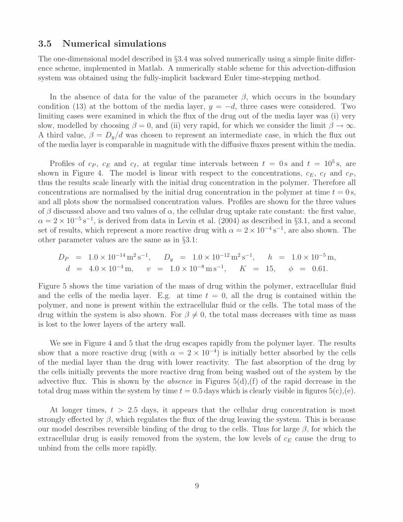
Figure 8: Restenosis in the absence of drug

Our model thus predicts that the artery will become completely blocked after a time tb, givenby:

tb =1

2log

R2

R2 − 1. (30)

This is clearly an unrealistic prediction, because as the artery becomes increasingly stenosed,the blood pressure will rise, compressing the wall tissue and hence our assumption of constantcell volume fraction may become invalid. However, tb gives us a rough timescale over which wecan expect the stenosis to become severe in untreated cases.

Our model may, however, provide a reasonable description of the earlier stages of restenosis.Using information from Buergler et al. (2000), which studied restenosis in pigs, we note thatafter 28 days, the lumenal diameter decreases by about 70% (i.e. a ≈ 0.3Rs) and the averagevalue of the ratio R∗/Rs = 1.2. Substituting these values into our equation for a above, we finda value for the parameter λ, of around 0.02 day−1. A plot of the dimensionless lumen radiusfor the above parameter values is shown in Figure 8.

4.2 Drug diffusion within the media tissue

We now turn to modelling the distribution of the drug within the new wall tissue - i.e. theregion a(t) ≤ r ≤ Rs. In order to keep our model as simple as possible, we will assume thatdiffusion, with coefficient D, is the dominant transport mechanism (this may in practice be apoor approximation, see §3.3). The drug will both decay naturally, and also be taken up by thecells; hence we postulate a sink term of the form (c1 + c2n0)c, where c1 and c2 are constants,and n0 is the volume fraction of live cells (as before, assumed constant). If we make the furtherassumption that the timescale of drug diffusion is much shorter than that for tissue growth (notunreasonable, given the drug diffusion timescale stated in §3.3 and the value of λ calculated

15

above) we arrive at the following equation for c:

∂2c

∂r2+

1

r

∂c

∂r− σ∗c = 0, (31)

where σ∗ = (c1+c2n0)D

. This is subject to the following boundary conditions:

c(Rs) = cs, c(a) = 0, (32)

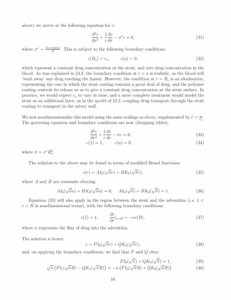
which represent a constant drug concentration at the stent, and zero drug concentration in theblood. As was explained in §3.2, the boundary condition at r = a is realistic, as the blood will‘wash away’ any drug reaching the lumen. However, the condition at r = Rs is an idealisation,representing the case in which the stent coating contains a great deal of drug, and the polymercoating controls its release so as to give a constant drug concentration at the stent surface. Inpractice, we would expect cs to vary in time, and a more complete treatment would model thestent as an additional layer, as in the model of §3.2, coupling drug transport through the stentcoating to transport in the artery wall.

We now nondimensionalise this model using the same scalings as above, supplemented by c = ccs

.The governing equation and boundary conditions are now (dropping tildes):

∂2c

∂r2+

1

r

∂c

∂r− σc = 0, (33)

c(1) = 1, c(a) = 0, (34)

where σ = σ∗R2s .

The solution to the above may be found in terms of modified Bessel functions:

c(r) = AI0(√

σr) + BK0(√

σr), (35)

where A and B are constants obeying:

AI0(√

σa) + BK0(√

σa) = 0, AI0(√

σ) + BK0(√

σ) = 1. (36)

Equation (33) will also apply in the region between the stent and the adventitia (i.e. 1 <r < R in nondimensional terms), with the following boundary conditions:

c(1) = 1,∂c

∂r|r=R = −κc(R), (37)

where κ represents the flux of drug into the adventitia.

The solution is hence:c = PI0(

√σr) + QK0(

√σr), (38)

and, on applying the boundary conditions, we find that P and Q obey:

PI0(√

σ) + QK0(√

σ) = 1, (39)√σ

(PI1(

√σR) − QK1(

√σR)

)= −κ

(PI0(

√σR) + QK0(

√σR)

)(40)

16

0.8

01.210.6

0.6

0.4

1

0.80.4

0.2

c

r

Figure 9: Drug concentration within theartery wall (κ = 1, σ = 0.1, a = 0.3, R = 1.2)

0.8

01.210.6

0.6

0.4

1

0.80.4

0.2

c

r

Figure 10: Drug concentration within theartery wall (κ = 1, σ = 10, a = 0.3, R = 1.2)

We recall from §3.1, that the uptake rate for the drug by the cells α is O(10−5s−1) and theradial diffusion coefficient D ∼ 10−12m2s−1; from (Buergler et al., 2000), we take Rs ∼ 10−3m.We hence estimate σ using the quantity αR2

s/D as being approximately 0.1. The parameter κ,which specifies the flux of drug from the media into the adventitia cannot be estimated fromthe literature, so we shall take κ = 1. We can thus plot the distribution of the drug for givenvalues of a; when a = 0.3, and other parameters take the values mentioned above, the solutionis as displayed in Figure 9. The effect of increasing the rate of drug consumption / decay (toσ = 10) is to give a distribution which is more strongly peaked close to the stent, as shown inFigure 10.

4.2.1 Drug present case: inhibition of cell proliferation

We now return to our model of section §4.1, modifying the equations to include the effect ofthe drug as an inhibitor of cell proliferation. Thus, the term g(n, c) now becomes:

g(n, c) =α1n0

1 + kc, (41)

where k is a constant which describes the ‘potency’ or ‘efficacy’ of the drug at inhibiting cellproliferation. Note that we still retain the simplifying assumption that the volume fraction ofcells is constant.

In the previous section, we found the solution for the drug distribution within the media interms of Bessel functions. However, if we were to substitute this solution into equation (22),we would be unable to make any analytical progress. Instead, we shall attempt to gain somequalitative insights by using linear approximations of the drug concentration profiles. In the

17

0.4

1

0

0.6

1.210.6 0.8

0.2

0.8

0.4

c

r

Figure 11: Exact and approximate solutionsfor c (κ = 1, σ = 0.1, a = 0.3)

0.8

0

1

0.6

1.21.10.9

0.2

0.4

10.7 0.8

c

r

Figure 12: Exact and approximate solutionsfor c (κ = 1, σ = 0.1, a = 0.6)

region a(t) < r < 1 (in dimensionless variables), we approximate c(r) by the line:

c =r − a

1 − a, (42)

where we have scaled concentrations with cs and lengths with Rs, as before. Similarly, in theregion 1 < r < R∗, we approximate c using the line:

c = 2 − r (43)

In Figures 11 and 12 we show the exact and approximate solutions for c for two values ofa (a = 0.3 and a = 0.6 respectively). We see that, for the parameter values chosen, the linearfunctions provide a reasonable approximation of the true solutions.

We now nondimensionalise equation (22), incorporating the new form for g (41) and the linearapproximation for c. We introduce a new scaling for the time, based on cell proliferation inthe drug free case (as the drug inhibits cell proliferation, this scaling is more convenient in thiscase). Thus, we set t = α1n0t and v = v/α1n0Rs, but the length and concentration scalingsremain unchanged from §4.2. We hence obtain:

1

r

∂(rv)

∂r=

1 − a

1 − k1a + k2r− β2, in a < r < 1 (44)

where k2 = kcs and β2 = β1(1 − n0)/α1n0 are dimensionless parameters. These represent theeffectiveness of the drug (a combination of its concentration and potency) and the relative rateof clearance of cellular debris respectively. For algebraic convenience, we have also introducedk1 = 1 + k2.

1

r

∂(rv)

∂r=

1

δ − k2r− β2, in 1 < r < R (45)

18

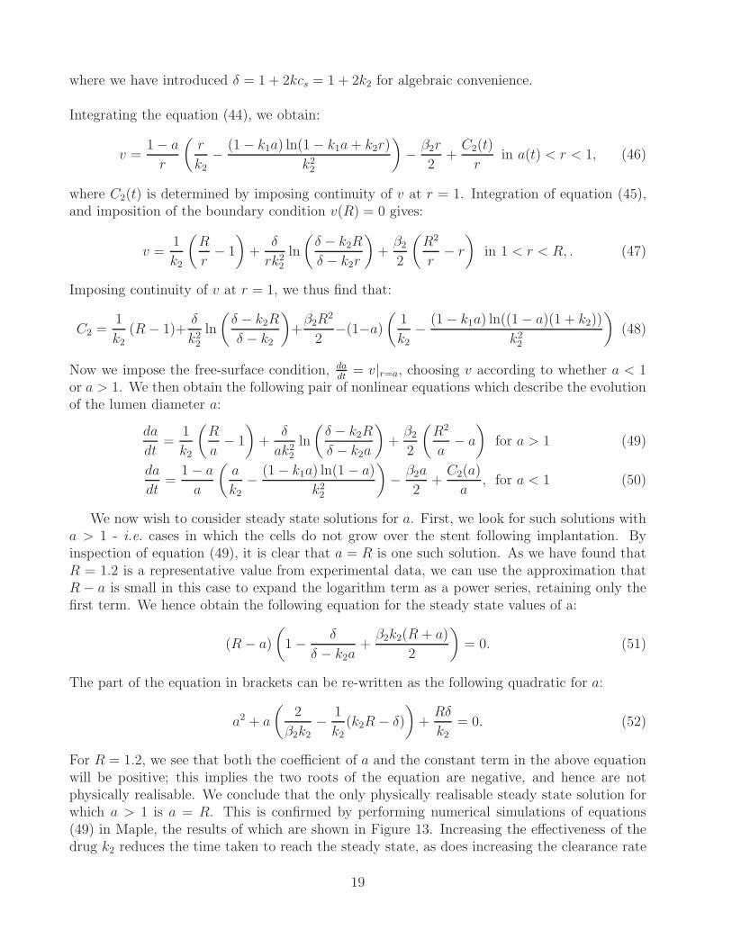
where we have introduced δ = 1 + 2kcs = 1 + 2k2 for algebraic convenience.

Integrating the equation (44), we obtain:

v =1 − a

r

(r

k2− (1 − k1a) ln(1 − k1a + k2r)

k22

)− β2r

2+

C2(t)

rin a(t) < r < 1, (46)

where C2(t) is determined by imposing continuity of v at r = 1. Integration of equation (45),and imposition of the boundary condition v(R) = 0 gives:

v =1

k2

(R

r− 1

)+

δ

rk22

ln

(δ − k2R

δ − k2r

)+

β2

2

(R2

r− r

)in 1 < r < R, . (47)

Imposing continuity of v at r = 1, we thus find that:

C2 =1

k2(R − 1)+

δ

k22

ln

(δ − k2R

δ − k2

)+

β2R2

2−(1−a)

(1

k2− (1 − k1a) ln((1 − a)(1 + k2))

k22

)(48)

Now we impose the free-surface condition, dadt

= v|r=a, choosing v according to whether a < 1or a > 1. We then obtain the following pair of nonlinear equations which describe the evolutionof the lumen diameter a:

da

dt=

1

k2

(R

a− 1

)+

δ

ak22

ln

(δ − k2R

δ − k2a

)+

β2

2

(R2

a− a

)for a > 1 (49)

da

dt=

1 − a

a

(a

k2− (1 − k1a) ln(1 − a)

k22

)− β2a

2+

C2(a)

a, for a < 1 (50)

We now wish to consider steady state solutions for a. First, we look for such solutions witha > 1 - i.e. cases in which the cells do not grow over the stent following implantation. Byinspection of equation (49), it is clear that a = R is one such solution. As we have found thatR = 1.2 is a representative value from experimental data, we can use the approximation thatR − a is small in this case to expand the logarithm term as a power series, retaining only thefirst term. We hence obtain the following equation for the steady state values of a:

(R − a)

(1 − δ

δ − k2a+

β2k2(R + a)

2

)= 0. (51)

The part of the equation in brackets can be re-written as the following quadratic for a:

a2 + a

(2

β2k2− 1

k2(k2R − δ)

)+

Rδ

k2= 0. (52)

For R = 1.2, we see that both the coefficient of a and the constant term in the above equationwill be positive; this implies the two roots of the equation are negative, and hence are notphysically realisable. We conclude that the only physically realisable steady state solution forwhich a > 1 is a = R. This is confirmed by performing numerical simulations of equations(49) in Maple, the results of which are shown in Figure 13. Increasing the effectiveness of thedrug k2 reduces the time taken to reach the steady state, as does increasing the clearance rate

19

1.15

1.2

40

1.1

1

1.05

60503010 200

a

t

Figure 13: Evolution of lumen diameter with R = 1.2, β2 = 1 and k2 = 1 (upper curve),k2 = 0.1 (lower curve)

of cellular debris, β2. However, if k2 or β2 are too small (i.e. the drug has little effect on cellproliferation, or cellular debris is allowed to accumulate), we find that a will decrease belowunity, and we must hence turn to equation (50).

Numerical simulations of equation (50) are displayed in Figure 14. We see that increasing theeffectiveness of the drug significantly reduces the rate of restenosis. A similar effect is noted forincreasing β2. Although, in this regime, total restenosis is eventually predicted by our model,in reality, the reduction in the rate of SMC proliferation would afford an opportunity for theendothelial lining of the artery to regrow, which would, we expect, prevent further restenosis.

5 Conclusions

In this report, we have described the development of models treating two problems related tothe introduction of a stent into an artery. In §3, we considered at the release of a drug from apolymer coated stent. Simple scaling arguments, described in §3.3 suggest that the proportionof the drug which is absorbed by the artery wall is dependent on the precise contact areabetween each wire of the stent and the underlying tissue. Because the contact problem requiresdetailed knowledge of the local biomechanics of a diseased artery wall, and knowledge of themechanical forces applied during stent insertion, it seems unlikely that mathematical modellingcan provide satisfactory results for this contact problem. However, the transport of the drugwithin the artery wall is quite amenable to mathematical modelling.

We established a simple model describing the advection and diffusion of the drug and itsuptake by cells in the media layer of the artery wall. We solved this model in a simplified onedimensional geometry. We found that the initial release of a drug from a drug coated stent,over times <2.5 days after stent insertion, is governed by the drug’s cell binding properties. At

20

0.8

1

6

0.6

0.4

14121040 2 8

a

t

Figure 14: Evolution of lumen diameter with R = 1.2, β2 = 0.5 and k2 = 1.1 (upper curve),k2 = 1.0 (lower curve)

later times, variation in the cellular drug concentration is largely accounted for by the trans-port of the drug to the outer layer of the artery wall. Future work could include the study ofmore complex geometries and more complex drug-cell binding kinetics. We note that severalpublished studies, listed in §2, have already made progress in these areas.

In §4.1, we treated the related problem of smooth muscle cell proliferation in a stentedartery, which can lead to restenosis. We showed, using our simple model, that drug-elutingstents can slow the rate of restenosis, or possibly eliminate the problem altogether, if the drugis sufficiently effective (in practice, there will be issues of toxicity, which we have not consideredhere). One of the most significant limitations of this model was the assumption of a constantdrug concentration on the surface of the stent. We described how a more complete treatmentwould include coupling of drug transport within the stent coating to that in the artery wall, asin the model of §3.2. Another limitation was the neglect of drug convection with the transmuralfluid flow, which, again was included in the model of §3.2. Such extensions are left to futurework.

References

F. Alexis, S. S. Venkatraman, S. K. Rath, and F. Boey. In vitro study of release mechanismsof paclitaxel and rapamycin from drug-incorporated biodegradable stent matrices. Journalof controlled release, 98:67–74, 2004.

J. M. Buergler, F. O. Tio, D. G. Schulz, M. M. Khan, W. Mazur, B. A. French, A. E. Raizner,and N. M. Ali. Use of nitric-oxide-eluting polymer coated coronary stents for prevention ofrestenosis in pigs. Coronary Artery Disease, 11:351–357, 2000.

21

R. Corti and J. J. Badimon. Biological aspects of vulnerable plaque. Current Opinion inCardiology, 17:616–625, 2002.

S. J. Franks and J. R. King. Interactions between a uniformly proliferating tumour and itssurroundings: uniform material properties. Math. Med. Biol., 20(1):47–89, 2003.

C.-W. Hwang and E. R. Edelman. Arterial ultrastructure influences transport of locally deliv-ered drugs. Circulation Research, 90:826–832, 2002.

C.-W. Hwang, D. Wu, and E. R. Edelman. Impact of transport and drug properties on the localpharmacology of drug-eluting stents. International Journal of Cardiovascular Interventions,5:7–12, 2003.

J. R. King and S. J. Franks. Mathematical analysis of some multi-dimensional tissue-growthmodels. Euro. J. App. Math., 15:273–295, 2004.

A.D. Levin, N. Vukmirovic, C.-W. Hwang, and E.R. Edelman. Specific binding to intracellularproteins determines arterial transport properties for rapamycin and paclitaxel. Proceedingsof the National Academy of Sciences of the USA, 101(25):9463–9467, 2004.

P. Libby. Changing concepts of atherogenesis. Journal of Internal Medicine, 247:349–358, 2000.

V. Montagano, S. Morosi, M. Dayar, A. Gomma, M. Atherton, M. Collins, and A. Redaelli.The link between restenosis and cardiovascular stent design: a study combining compuationalfluid dnamics with computer aided design. Internal Medicine, 11:14–23, 2003.

D. V. Sakharov, L. V. Kalachev, and D. C. Rijken. Numerical simulation of local pharmacoki-netics of a drug after intravascular delivery with an eluting stent. Journal of Drug Targeting,10(6):507–513, 2002.

J. E. Sousa, P. W. Serruys, and M. A. Costa. New frontiers in cardiology. drug-eluting stents:part i. Circulation, 107:2274–2279, 2003.

X. M. Yuan, U. T. Brunk, and L. Hazell. The morphology and natural history of atherosclerosis.In Dean R T and Kelly D T, editors, Atherosclerosis. Gene expression, cell interactions andoxidation, pages 1–23. Oxford University Press, New York, USA, 2000.

P. Zunino. Multidimensional pharmacokinetic models applied to the design of drug-elutingstents. Cardiovascular engineering: An International Journal, 4(2):181–191, 2004.

22