Arrhythmia Care Co-ordinator Services - NHS Alliance 2012

Inferences Based on a Single Sample: Estimation with Confidence Intervals Chapter 5

5.2 a. zα/2 = 1.96, using Table IV, Appendix B, P(0 ≤ z ≤ 1.96) = .4750. Thus, α/2 = .5000 − .4750 = .025, α = 2(.025) = .05, and 1 - α = 1 - .05 = .95. The confidence level is

100% × .95 = 95%. b. zα/2 = 1.645, using Table IV, Appendix B, P(0 ≤ z ≤ 1.645) = .45. Thus, α/2 = .50 − .45 =

.05, α = 2(.05) = .1, and 1 − α = 1 − .1 = .90. The confidence level is 100% × .90 = 90%. c. zα/2 = 2.575, using Table IV, Appendix B, P(0 ≤ z ≤ 2.575) = .495. Thus, α/2 = .500 −

.495 = .005, α = 2(.005) = .01, and 1 − α = 1 − .01 = .99. The confidence level is 100% × .99 = 99%. d. zα/2 = 1.282, using Table IV, Appendix B, P(0 ≤ z ≤ 1.282) = .4. Thus, α/2 = .5 − .4 = .1,

α = 2(.1) = .2, and 1 − α = 1 − .2 = .80. The confidence level is 100% × .80 = 80%. e. zα/2 = .99, using Table IV, Appendix B, P(0 ≤ z ≤ .99) = .3389. Thus, α/2 = .5000 − .3389

= .1611, α = 2(.1611) = .3222, and 1 − α = 1 − .3222 = .6778. The confidence level is 100% × .6778 = 67.78%.

5.4 a. For confidence coefficient .95, α = .05 and α/2 = .05/2 = .025. From Table IV, Appendix

B, z.025 = 1.96. The confidence interval is:

x ± z.025sn

⇒ 25.9 ± 1.96 2.790

⇒ 25.9 ± .56 ⇒ (25.34, 26.46)

b. For confidence coefficient .90, α = .10 and α/2 = .10/2 = .05. From Table IV, Appendix


x ± z.05sn

⇒ 25.9 ± 1.645 2.790

⇒ 25.9 ± .47 ⇒ (25.43, 26.37)

c. For confidence coefficient .99, α = .01 and α/2 = .01/2 = .005. From Table IV, Appendix


x ± z.005sn

⇒ 25.9 ± 2.58 2.790

⇒ 25.9 ± .73 ⇒ (25.17, 26.63)

5.6 If we were to repeatedly draw samples from the population and form the interval x ± 1.96 xσ

each time, approximately 95% of the intervals would contain μ. We have no way of knowing whether our interval estimate is one of the 95% that contain μ or one of the 5% that do not.

Inferences Based on a Single Sample: Estimation with Confidence Intervals 137

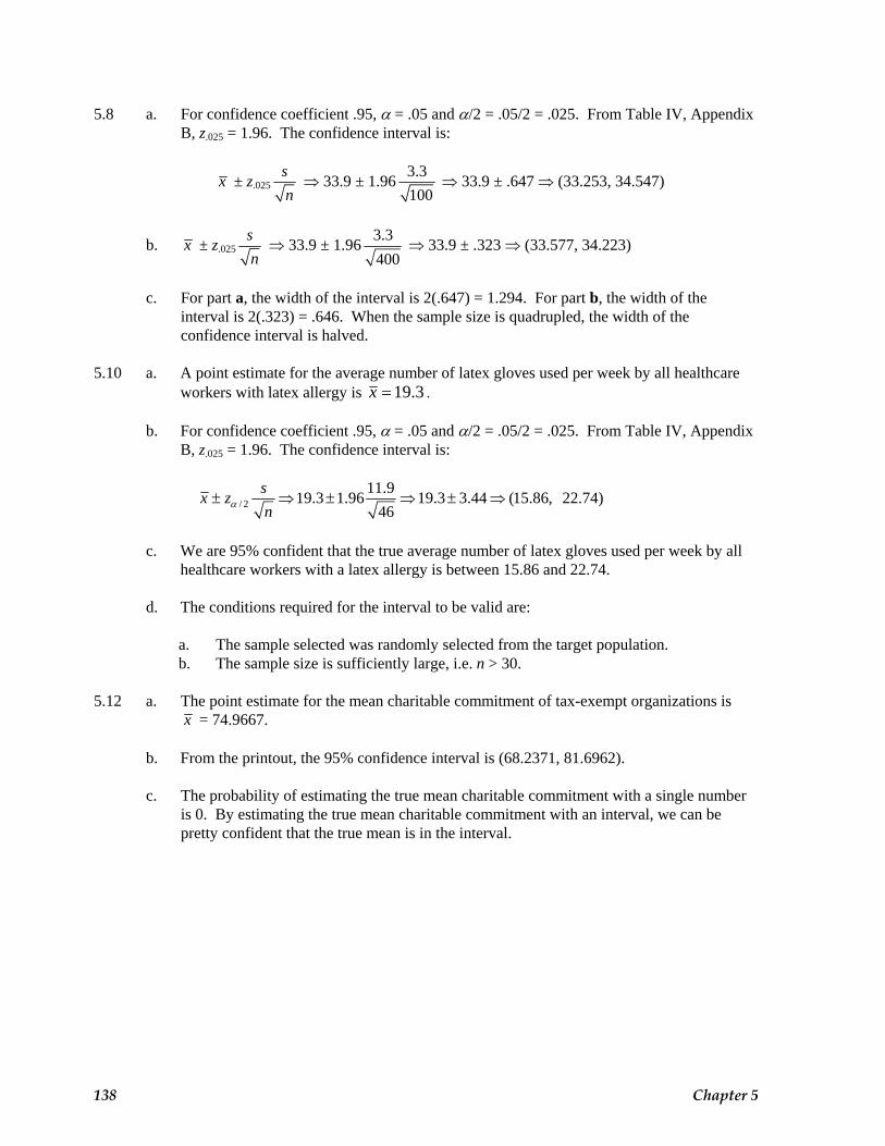
5.8 a. For confidence coefficient .95, α = .05 and α/2 = .05/2 = .025. From Table IV, Appendix B, z.025 = 1.96. The confidence interval is:

x ± z.025sn

⇒ 33.9 ± 1.96 3.3100

⇒ 33.9 ± .647 ⇒ (33.253, 34.547)

b. x ± z.025sn

⇒ 33.9 ± 1.96 3.3400

⇒ 33.9 ± .323 ⇒ (33.577, 34.223)

c. For part a, the width of the interval is 2(.647) = 1.294. For part b, the width of the

interval is 2(.323) = .646. When the sample size is quadrupled, the width of the confidence interval is halved.

5.10 a. A point estimate for the average number of latex gloves used per week by all healthcare

workers with latex allergy is 3.19=x .

b. For confidence coefficient .95, α = .05 and α/2 = .05/2 = .025. From Table IV, Appendix B, z.025 = 1.96. The confidence interval is:

/ 211.919.3 1.96 19.3 3.44 (15.86, 22.74)

46sx znα± ⇒ ± ⇒ ± ⇒

c. We are 95% confident that the true average number of latex gloves used per week by all

healthcare workers with a latex allergy is between 15.86 and 22.74.

d. The conditions required for the interval to be valid are:

a. The sample selected was randomly selected from the target population. b. The sample size is sufficiently large, i.e. n > 30.

5.12 a. The point estimate for the mean charitable commitment of tax-exempt organizations is x = 74.9667.

b. From the printout, the 95% confidence interval is (68.2371, 81.6962). c. The probability of estimating the true mean charitable commitment with a single number

is 0. By estimating the true mean charitable commitment with an interval, we can be pretty confident that the true mean is in the interval.

138 Chapter 5

5.14 Using MINITAB, the descriptive statistics are:

Descriptive Statistics: r

Variable N Mean Median TrMean StDev SE Mean r 34 0.4224 0.4300 0.4310 0.1998 0.0343

Variable Minimum Maximum Q1 Q3 r -0.0800 0.7400 0.2925 0.6000

For confidence coefficient .95, α = .05 and α/2 = .05/2 = .025. From Table IV, Appendix B, z.025 = 1.96. The confidence interval is:

/ 2.1998.4224 1.96 .4224 .0672

34(.3552, .4895)

sx znα± ⇒ ± ⇒ ±

⇒

We are 95% confident that the mean value of r is between .3552 and .4895.

5.16 a. Using MINITAB, the descriptive statistics are:

Descriptive Statistics: Rate

Variable N Mean Median TrMean StDev SE Mean Rate 30 79.73 80.00 80.15 5.96 1.09

Variable Minimum Maximum Q1 Q3 Rate 60.00 90.00 76.75 84.00


/ 25.9679.73 1.645 79.73 1.79

30(77.94, 81.52)

sx znα± ⇒ ± ⇒ ±

⇒

b. We are 90% confident that the mean participation rate for all companies that have 401(k)

plans is between 77.94% and 81.52%. c. We must assume that the sample size (n = 30) is sufficiently large so that the Central

Limit Theorem applies. d. Yes. Since 71% is not included in the 90% confidence interval, it can be concluded that this

company's participation rate is lower than the population mean. e. The center of the confidence interval is . If 60% is changed to 80%, the value of will

increase, thus indicating that the center point will be larger. The value of s2 will decrease if 60% is replaced by 80%, thus causing the width of the interval to decrease.


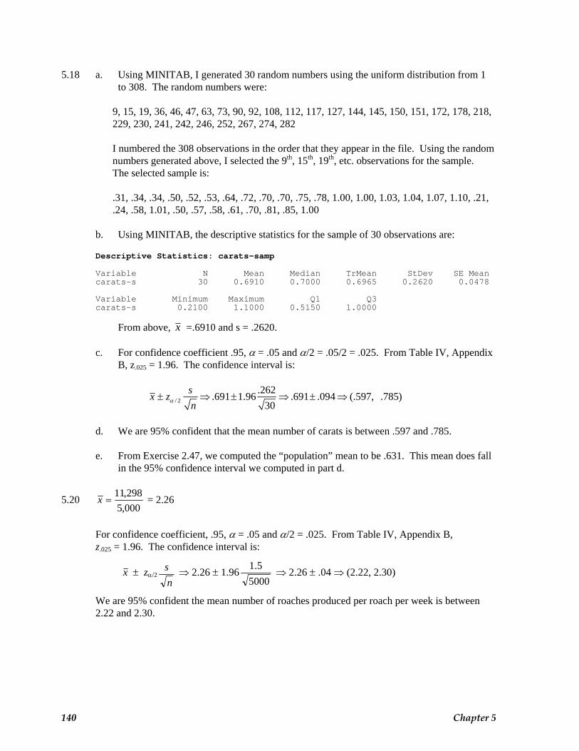
5.18 a. Using MINITAB, I generated 30 random numbers using the uniform distribution from 1 to 308. The random numbers were:

9, 15, 19, 36, 46, 47, 63, 73, 90, 92, 108, 112, 117, 127, 144, 145, 150, 151, 172, 178, 218, 229, 230, 241, 242, 246, 252, 267, 274, 282

I numbered the 308 observations in the order that they appear in the file. Using the random numbers generated above, I selected the 9th, 15th, 19th, etc. observations for the sample. The selected sample is:

.31, .34, .34, .50, .52, .53, .64, .72, .70, .70, .75, .78, 1.00, 1.00, 1.03, 1.04, 1.07, 1.10, .21, .24, .58, 1.01, .50, .57, .58, .61, .70, .81, .85, 1.00

b. Using MINITAB, the descriptive statistics for the sample of 30 observations are:

Descriptive Statistics: carats-samp

Variable N Mean Median TrMean StDev SE Mean carats-s 30 0.6910 0.7000 0.6965 0.2620 0.0478

Variable Minimum Maximum Q1 Q3 carats-s 0.2100 1.1000 0.5150 1.0000

From above, x =.6910 and s = .2620.

c. For confidence coefficient .95, α = .05 and α/2 = .05/2 = .025. From Table IV, Appendix


/ 2.262.691 1.96 .691 .094 (.597, .785)

30sx znα± ⇒ ± ⇒ ± ⇒

d. We are 95% confident that the mean number of carats is between .597 and .785.

e. From Exercise 2.47, we computed the “population” mean to be .631. This mean does fall

in the 95% confidence interval we computed in part d.

5.20 000,5298,11

=x = 2.26

For confidence coefficient, .95, α = .05 and α/2 = .025. From Table IV, Appendix B,

z.025 = 1.96. The confidence interval is:

x ± zα/2ns ⇒ 2.26 ± 1.96

50005.1 ⇒ 2.26 ± .04 ⇒ (2.22, 2.30)

We are 95% confident the mean number of roaches produced per roach per week is between

2.22 and 2.30.

140 Chapter 5

5.22 a. If x is normally distributed, the sampling distribution of x is normal, regardless of the sample size.

b. If nothing is known about the distribution of x, the sampling distribution of x is

approximately normal if n is sufficiently large. If n is not large, the distribution of x is unknown if the distribution of x is not known.

5.24 a. P(t ≥ t0) = .025 where df = 11 t0 = 2.201 b. P(t ≥ t0) = .01 where df = 9 t0 = 2.821 c. P(t ≤ t0) = .005 where df = 6 Because of symmetry, the statement can be rewritten P(t ≥ −t0) = .005 where df = 6 t0 = −3.707 d. P(t ≤ t0) = .05 where df = 18 t0 = −1.734 5.26 For this sample,

156716

xx

n= =∑ = 97.9375

s2 =

( )22

2 1567155,86716

1 16 1

xx

nn

− −=

− −

∑∑ = 159.9292

s = 2s = 12.6463 a. For confidence coefficient, .80, α = 1 − .80 = .20 and α/2 = .20/2 = .10. From Table VI,

Appendix B, with df = n − 1 = 16 − 1 = 15, t.10 = 1.341. The 80% confidence interval for μ is:

x ± t.10sn

⇒ 97.94 ± 1.341 12.646316

⇒ 97.94 ± 4.240 ⇒ (93.700, 102.180)

b. For confidence coefficient, .95, α = 1 − .95 = .05 and α/2 = .05/2 = .025. From Table VI,

Appendix B, with df = n − 1 = 24 − 1 = 23, t.025 = 2.131. The 95% confidence interval for μ is:

x ± t.025sn

⇒ 97.94 ± 2.131 12.646316

⇒ 97.94 ± 6.737 ⇒ (91.203, 104.677)

The 95% confidence interval for μ is wider than the 80% confidence interval for μ found

in part a.


c. For part a:

We are 80% confident that the true population mean lies in the interval 93.700 to 102.180.

For part b:

We are 95% confident that the true population mean lies in the interval 91.203 to 104.677.

The 95% confidence interval is wider than the 80% confidence interval because the more

confident you want to be that μ lies in an interval, the wider the range of possible values. 5.28 a. Using MINITAB, the descriptive statistics are: Descriptive Statistics: MTBE Variable N N* Mean SE Mean StDev Minimum Q1 Median Q3 Maximum MTBE 12 0 97.2 32.8 113.8 8.00 12.0 50.5 146.0 367.0 A point estimate for the true mean MTBE level for all well sites located near the New

Jersey gasoline service station is 97.2x = . b. For confidence coefficient .99, α = .01 and α/2 = .01/2 = .005. From Table VI, Appendix

B, with df = n – 1 = 12 – 1 = 11, t.005 = 3.106. The 99% confidence interval is:

.005113.897.2 3.106 97.2 102.04 ( 4.84, 199.24)

12sx tn

± ⇒ ± ⇒ ± ⇒ −

We are 99% confident that the true mean MTBE level for all well sites located near the New Jersey gasoline service station is between −4.84 and 199.24.

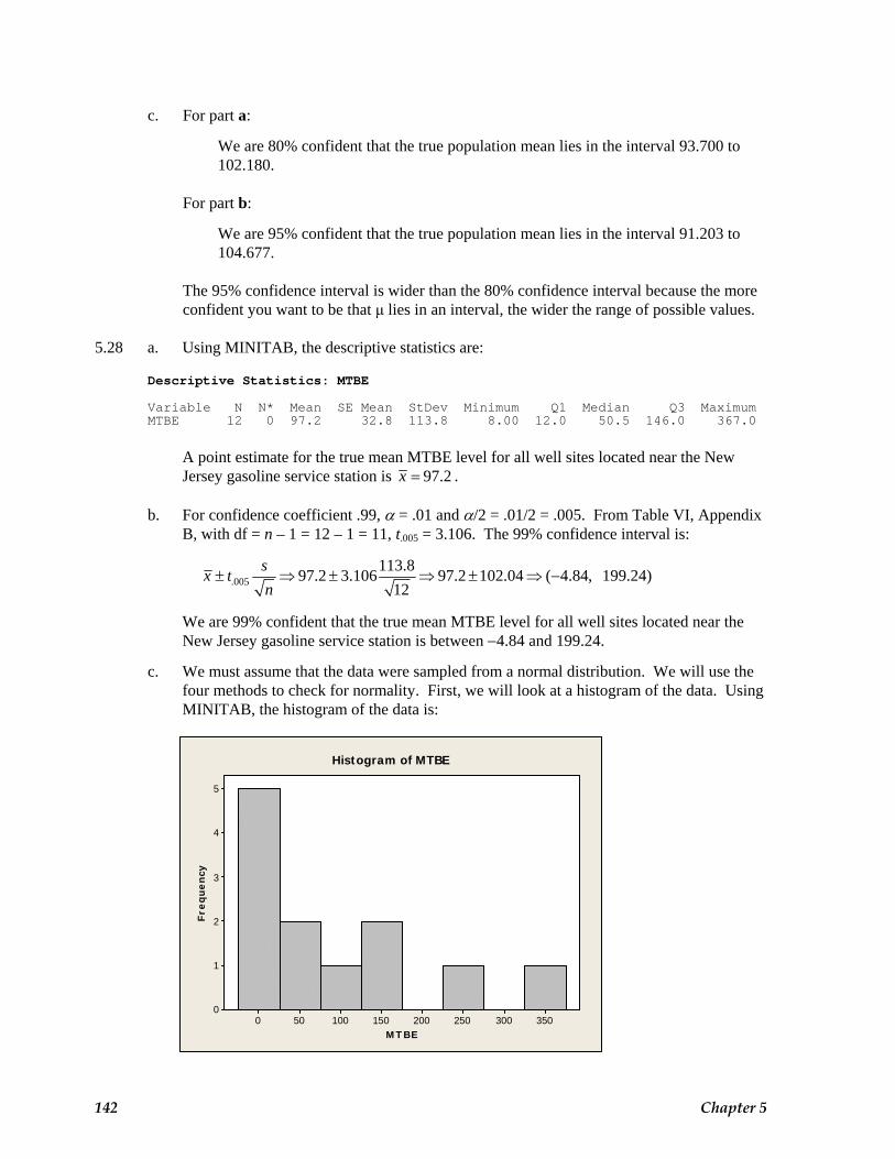
c. We must assume that the data were sampled from a normal distribution. We will use the four methods to check for normality. First, we will look at a histogram of the data. Using MINITAB, the histogram of the data is:

MT BE

Fre

qu

en

cy

350300250200150100500

5

4

3

2

1

0

Histogram of MTBE

142 Chapter 5

From the histogram, the data do not appear to be mound-shaped. This indicates that the data may not be normal.

Next, we look at the intervals , 2 , 3x s x s x s± ± ± . If the proportions of observations falling in each interval are approximately .68, .95, and 1.00, then the data are approximately normal. Using MINITAB, the summary statistics are:

97.2 113.8 ( 16.6, 211.0)x s± ⇒ ± ⇒ − 10 of the 12 values fall in this interval. The proportion is .83. This is not very close to the .68 we would expect if the data were normal.

2 97.2 2(113.8) 97.2 227.6 ( 130.4, 324.8)x s± ⇒ ± ⇒ ± ⇒ − 11 of the 12 values fall in this interval. The proportion is .92. This is a somewhat smaller than the .95 we would expect if the data were normal.

2 97.2 3(113.8) 97.2 341.4 ( 244.2, 438.6)x s± ⇒ ± ⇒ ± ⇒ − 12 of the 12 values fall in this interval. The proportion is 1.00. This is exactly the 1.00 we would expect if the data were normal.

From this method, it appears that the data may not be normal.

Next, we look at the ratio of the IQR to s. IQR = QU – QL = 146.0 – 12.0 = 134.0.

IQR 134.0 1.18s 113.8

= = This is somewhat smaller than the 1.3 we would expect if the data

were normal. This method indicates the data may not be normal.

Finally, using MINITAB, the normal probability plot is:

MT BE

Pe

rce

nt

5004003002001000-100-200-300

99

95

90

80

70

60

50

40

30

20

10

5

1

Mean

0.012

97.17StDev 113.8

N 12AD 0.929P-Value

Probability Plot of MTBENormal - 95% C I

Since the data do not form a fairly straight line, the data may not be normal. From above, the all methods indicate the data may not be normal. It appears that the data probably are not normal.


5.30 We must assume that the distribution of the LOS's for all patients is normal. a. For confidence coefficient .90, α = 1 − .90 = .10 and α/2 = .10/2 = .05. From Table VI,

Appendix B, with df = n − 1 = 20 − 1 = 19, t.05 = 1.729. The 90% confidence interval is:

.05sx tn

± ⇒ 3.8 ± 1.7291.220

⇒ 3.8 ± .464 ⇒ (3.336, 4.264)

b. We are 90% confident that the mean LOS is between 3.336 and 4.264 days. c. “90% confidence” means that if repeated samples of size n are selected from a population and

90% confidence intervals are constructed, 90% of all intervals thus constructed will contain the population mean.

5.32 a. The 95% confidence interval for the mean surface roughness of coated interior pipe is (1.63580, 2.12620).

b. No. Since 2.5 does not fall in the 95% confidence interval, it would be very unlikely that the average surface roughness would be as high as 2.5 micrometers.

5.34 a. The population is the set of all DOT permanent count stations in the state of Florida. b. Yes. There are several types of routes included in the sample. There are 3 recreational

areas, 7 rural areas, 5 small cities, and 5 urban areas.

c. Using MINITAB, the descriptive statistics are: Descriptive Statistics: 30th hour, 100th hour

Variable N Mean Median TrMean StDev SE Mean 30th hou 20 2206 2064 2165 1224 274 100th ho 20 2096 1999 2048 1203 269

Variable Minimum Maximum Q1 Q3 30th hou 252 4905 1429 3068 100th ho 229 4815 1318 2877

For confidence coefficient .95, α = .05 and α/2 = .05/2 = .025. From Table VI, Appendix B, with df = n – 1 = 20 – 1 = 19, t.025 = 2.093. The 95% confidence interval is:

.0251,2242,206 2.093 2,206 572.84 (1,633.16, 2,778.84)

20sx tn

± ⇒ ± ⇒ ± ⇒

We are 95% confident that the mean traffic count at the 30th highest hour is between 1,633.16 and 2,778.84.

d. We must assume that the distribution of the traffic counts at the 30th highest hour is

normal. From the stem-and-leaf display, the data look fairly mound-shaped. Thus, the assumption of normality is probably met.

144 Chapter 5

e. For confidence coefficient .95, α = .05 and α/2 = .05/2 = .025. From Table VI, Appendix B, with df = n – 1 = 20 – 1 = 19, t.025 = 2.093. The 95% confidence interval is:

.0251,2032,096 2.093 2,096 563.01 (1,532.99, 2,659.01)

20sx tn

± ⇒ ± ⇒ ± ⇒

We are 95% confident that the mean traffic count at the 100th highest hour is between 1,532.99 and 2,659.01.

We must assume that the distribution of the traffic counts at the 100th highest hour is

normal. From the stem-and-leaf display, the data look fairly mound-shaped. Thus, the assumption of normality is probably met.

f. If μ = 2,700, it is very possible that it is the mean count for the 30th highest hour. It falls

in the 95% confidence interval for the mean count for the 30th highest hour. It is not very likely that the mean count for the 100th highest hour is 2,700. It does not fall in the 95% confidence interval for the mean count for the 100th highest hour. (See parts c and e above.)

5.36 By the Central Limit Theorem, the sampling distribution of is approximately normal with

mean p̂μ = p and standard deviation p̂pqn

σ = .

5.38 a. The sample size is large enough if the interval p̂ ± ˆ3 pσ does not include 0 or 1.

p̂ ± ˆ3 pσ ⇒ p̂ ± 3 pqn

⇒ p̂ ± ˆ ˆ

3 pqn

⇒ .88 ± .88(1 .88)121− ⇒ .88 ± .089

⇒ (.791, .969) Since the interval lies within the interval (0, 1), the normal approximation will be

adequate. b. For confidence coefficient .90, α = .10 and α/2 = .05. From Table IV, Appendix B,

z.05 = 1.645. The 90% confidence interval is:

ˆ .05pqp z n

± ⇒ p̂ ± 1.645ˆ ˆpqn

⇒ .88 ± 1.645 .88(.12)1.645121

⇒ .88 ± .049

⇒ (.831, .929) c. We must assume that the sample is a random sample from the population of interest.


5.40 a. Of the 50 observations, 15 like the product ⇒ 15ˆ30

p = = .30.

To see if the sample size is sufficiently large:

p̂ ± 3 p̂σ ≈ p̂ ± 3ˆ ˆpqn

⇒ .3 ± .3(.7)350

⇒ .3 ± .194 ⇒ (.106, .494)

Since this interval is wholly contained in the interval (0, 1), we may conclude that the

normal approximation is reasonable. For the confidence coefficient .80, α = .20 and α/2 = .10. From Table IV, Appendix B,

z.10 = 1.28. The confidence interval is:

p̂ ± z.10ˆ ˆpqn

⇒ .3 ± 1.28 .3(.7)50

⇒ .3 ± .083 ⇒ (.217, .383)

b. We are 80% confident the proportion of all consumers who like the new snack food is

between .217 and .383. 5.42 a. The point estimate of p is ˆ .11p = .

b. To see if the sample size is sufficiently large:

ˆˆ ˆ .11(.89)ˆ ˆ3 3 .11 3 .11 .077 (.033, .187)

150ppqp pn

σ± ≈ ± ⇒ ± ⇒ ± ⇒

Since the interval is wholly contained in the interval (0, 1), we may conclude that the normal approximation is reasonable.


.025ˆ ˆ .11(.89)ˆ .11 1.645 .11 .05 (.06, .16)

150pqp zn

± ⇒ ± ⇒ ± ⇒

c. We are 95% confident that the true proportion of MSDS that are satisfactorily completed

is between .06 and .16.

5.44 a. The point estimate of p is 16ˆ .052308

xpn

= = = .


ˆˆ ˆ .052(.948)ˆ ˆ3 3 .052 3 .052 .038 (.014, .090)

308ppqp pn

σ± ≈ ± ⇒ ± ⇒ ± ⇒


146 Chapter 5


.05ˆ ˆ .052(.948)ˆ .052 2.58 .052 .033 (.019, .085)

308pqp zn

± ⇒ ± ⇒ ± ⇒

We are 99% confident that the true proportion of diamonds for sale that are classified as “D” color is between .019 and .085.

b. The point estimate of p is 81ˆ .263308

xpn

= = = .


ˆˆ ˆ .263(.737)ˆ ˆ3 3 .263 3 .263 .075 (.188, .338)

308ppqp pn

σ± ≈ ± ⇒ ± ⇒ ± ⇒


For confidence coefficient .99, α = .01 and α/2 = .01/2 = .005. From Table IV, Appendix


.05ˆ ˆ .263(.737)ˆ .263 2.58 .263 .065 (.198, .328)

308pqp zn

± ⇒ ± ⇒ ± ⇒

We are 99% confident that the true proportion of diamonds for sale that are classified as “VS1” clarity, is between .198 and .328.

5.46 a. The population is all senior human resource executives at U.S. companies.

b. The population parameter of interest is p, the proportion of all senior human resource executives at U.S. companies who believe that their hiring managers are interviewing too many people to find qualified candidates for the job.

c. The point estimate of p is 211ˆ .42502

xpn

= = = . To see if the sample size is sufficiently

large:

ˆˆ ˆ .42(.58)ˆ ˆ3 3 .42 3 .42 .066 (.354, .486)

502ppqp pn

σ± ≈ ± ⇒ ± ⇒ ± ⇒



d. For confidence coefficient .98, α = .02 and α/2 = .02/2 = .01. From Table IV, Appendix B, z.01 = 2.33. The confidence interval is:

.01ˆ ˆ .42(.58)ˆ .42 2.33 .42 .051 (.369, .471)

502pqp zn

± ⇒ ± ⇒ ± ⇒

We are 98% confident that the true proportion of all senior human resource executives at

U.S. companies who believe that their hiring managers are interviewing too many people to find qualified candidates for the job is between .369 and .471.

e. A 90% confidence interval would be narrower. If the interval was narrower, it would contain fewer values, thus, we would be less confident.

5.48 a. The point estimate of p is p̂ = x/n = 35/55 = .636. b. We must check to see if the sample size is sufficiently large:

p̂ ± ˆ3 pσ ≈ p̂ ± ˆ ˆ

3 pqn

⇒ .636 ± .636(.364)355

⇒ .636 ± .195 ⇒ (.441, .831)

Since the interval is wholly contained in the interval (0, 1) we may assume that the

normal approximation is reasonable. For confidence coefficient, .99, α = .01 and α/2 = .01/2 = .005. From Table IV,

Appendix B, z.005 = 2.575. The confidence interval is:

p̂ ± z.005ˆ ˆpqn

⇒ .636 ± .636(.364)2.57555

⇒ .636 ± .167 ⇒ (.469, .803)

c. We are 99% confident that the true proportion of fatal accidents involving children is

between .469 and .803. d. The sample proportion of children killed by air bags who were not wearing seat belts or

were improperly restrained is 24/35 = .686. This is rather large proportion. Whether a child is killed by an airbag could be related to whether or not he/she was properly restrained. Thus, the number of children killed by air bags could possibly be reduced if the child were properly restrained.

5.50 The point estimate of p is 36ˆ .43483

xpn

= = = .


ˆˆ ˆ .434(.566)ˆ ˆ3 3 .434 3 .434 .163 (.271, .597)

83ppqp pn

σ± ≈ ± ⇒ ± ⇒ ± ⇒


148 Chapter 5


.025ˆ ˆ .434(.566)ˆ .434 1.96 .434 .107 (.327, .541)

83pqp zn

± ⇒ ± ⇒ ± ⇒

We are 95% confident that the true proportion of healthcare workers with latex allergies actually suspects the he or she actually has the allergy is between .327 and .541.

5.52 To compute the necessary sample size, use

n = ( )2 2/ 2

2

zSE

α σ where α = 1 − .95 = .05 and α/2 = .05/2 = .025.

From Table IV, Appendix B, z.025 = 1.96. Thus,

n = 2

2

(1.96) (7.2).3

= 307.328 ≈ 308

You would need to take 308 samples. 5.54 a. To compute the needed sample size, use:

n = ( )2/ 2

2

pqzSEα where z.025 = 1.96 from Table IV, Appendix B.

Thus, n = 2

2

(1.96) (.2)(.8).08

= 96.04 ≈ 97

You would need to take a sample of size 97. b. To compute the needed sample size, use:

n = ( )2/ 2

2

pqzSEα =

2

2

(1.96 (.5)(.5)).08

= 150.0625 ≈ 151

You would need to take a sample of size 151. 5.56 a. For a width of 5 units, SE = 5/2 = 2.5. To compute the needed sample size, use

n = ( )2 2/ 2

2

zSEα σ where α = 1 − .95 = .05 and α/2 = .025.



n = 2 2

2

(1.96) (14)2.5

= 120.47 ≈ 121

You would need to take 121 samples at a cost of 121($10) = $1210. Yes, you do have sufficient funds. b. For confidence coefficient .90, α = 1 − .90 = .10 and α/2 = .10/2 = .05. From Table IV,

Appendix B, z.05 = 1.645.

n = 2 2

2

(1.645) (14)2.5

= 84.86 ≈ 85

You would need to take 85 samples at a cost of 85($10) = $850. You still have sufficient funds but have an increased risk of error. 5.58 The sample size will be larger than necessary for any p other than .5. 5.60 a. The confidence level desired by the researchers is 90%.

b. The sampling error desired by the researchers is SE = .05. c. For confidence coefficient .90, α = .10 and α/2 = .10/2 = .05. From Table IV,

Appendix B, z.05 = 1.645. From the problem, we will use 64ˆ .604106

xpn

= = =

to estimate p. Thus,

2 2

/ 22 2

( ) 1.645 .604(.396) 258.9 259( ) .05

z pqnSE

α= = = ≈

Thus, we would need a sample of size 259. 5.62 For confidence coefficient .95, α = .05 and α/2 = .05/2 = .025. From Table IV, Appendix B,

z.025 = 1.96. For this study,

n = 2 2 2 2

/ 22 2

( ) 1.96 (5)1

zSE

α σ≈ = 96.04 ≈ 97

The sample size needed is 97.

150 Chapter 5

5.64 For confidence coefficient .90, α = .10 and α/2 = .05. From Table IV, Appendix B, z.05 = 1.645.

For a width of .06, SE = .06/2 = .03

The sample size is n = 2

/ 22

( )z pSE

α q = 2

2

(.1645) (.17)(.83).03

= 424.2 ≈ 425

You would need to take n = 425 samples. 5.66 To compute the necessary sample size, use

n = 2 2

/ 22

( )zSE

α σ where α = 1 − .90 = .10 and α/2 = .05.


n = 2 2

2

(1.645) (10)1

= 270.6 ≈ 271

5.68 a. To compute the needed sample size, use

n = 2 2

/ 22

( )zSE

α σ where α = 1 − .90 = .10 and α/2 = .05.


n = 2 2

2

(1.645) (2).1

= 1,082.41 ≈ 1,083

b. As the sample size decreases, the width of the confidence interval increases. Therefore, if

we sample 100 parts instead of 1,083, the confidence interval would be wider. c. To compute the maximum confidence level that could be attained meeting the

management's specifications,

n = 2 2

/ 22

( )zSE

α σ ⇒ 100 = 2

/ 22

( )(2).1

zα ⇒ 2/ 2

100(.01)( )4

zα = = .25 ⇒ zα/2 = .5

Using Table IV, Appendix B, P(0 ≤ z ≤ .5) = .1915. Thus, α/2 = .5000 − .1915 = .3085,

α = 2(.3085) = .617, and 1 − α = 1 − .617 = .383. The maximum confidence level would be 38.3%.


5.70 xN n=

Nnσσ −

a. 200 2500 100025001000

x σ−

= = 4.90

b. 200 5000 100050001000x

σ −= = 5.66

c. 200 10,000 100010,0001000x

= σ − = 6.00

d. 200 100,000 1000100,0001000x

σ −= = 6.293

5.72 a. For n = 36, with the finite population correction factor:

24 5000 64ˆ / 3 .9872500064x

N n s n N

σ⎛ ⎞ ⎛ ⎞− −

= = =⎜ ⎟ ⎜ ⎟⎜ ⎟ ⎜ ⎟⎝ ⎠ ⎝ ⎠

= 2.9807

without the finite population correction factor:

24ˆ /64x s n σ = = = 3

ˆ xσ without the finite population correction factor is slightly larger. b. For n = 400, with the finite population correction factor:

24 5000 400ˆ / 1.2 .925000400x

N n s n N

σ⎛ ⎞ ⎛ ⎞− −

= = =⎜ ⎟ ⎜ ⎟⎜ ⎟ ⎜ ⎟⎝ ⎠ ⎝ ⎠

= 1.1510

without the finite population correction factor:

24ˆ /400x s n σ = = = 1.2

c. In part a, n is smaller relative to N than in part b. Therefore, the finite population

correction factor did not make as much difference in the answer in part a as in part b. 5.74 An approximate 95% confidence interval for μ is:

x ± ˆ2 xσ ⇒ x ± 2 s N nNn− ⇒ 422 ± 2 14 375 40

37540 −

⇒ 422 ± 4.184 ⇒ (417.816, 426.184)

152 Chapter 5

5.76 a. For N = 2,193, n = 223, x =116,754, and s = 39,185, the 95% confidence interval is:

39,185 2,193 223ˆ2 2 116,754 2

2,193223116,754 4,974.06 (111,779.94, 121,728.06)

xs N nx x

Nnσ − −

± ⇒ ± ⇒ ±

⇒ ± ⇒

b. We are 95% confident that the mean salary of all vice presidents who subscribe to

Quality Progress is between $111,777.94 and $121,728.06. 5.78 a. The population of interest is the set of all households headed by women that have incomes

of $25,000 or more in the database. b. Yes. Since n/N = 1,333/25,000 = .053 exceeds .05, we need to apply the finite population

correction. c. The standard error for p̂ should be:

ˆˆ ˆ(1 ) .708(1 .708) 25,000 1,333ˆ

1333 25,000pp p N n

n Nσ − − − −⎛ ⎞⎛ ⎞= =⎜ ⎟ ⎜ ⎟⎝ ⎠ ⎝ ⎠

= .012

d. For confidence coefficient .90, α = 1 − .90 = .10 and α/2 = .10/2 = .05. From Table

IV, Appendix B, z.05 = 1.645. The approximate 90% confidence interval is: p̂ ± ˆˆ1.645 pσ ⇒ .708 ± 1.645(.012) ⇒ (.688, .728)

5.80 For N = 1,500, n = 35, x = 1, and s = 124, the 95% confidence interval is:

x ± ˆ2 xσ ⇒ x ± 2 s N nNn−⎛ ⎞

⎜ ⎟⎝ ⎠

⇒ 1 ± 124 1,500 352

1,50035−⎛ ⎞

⎜ ⎟⎝ ⎠

⇒ 1 ± 41.43

⇒ (−40.43, 42.43) We are 95% confident that the mean error of the new system is between -$40.43 and $42.43. 5.82 a. For a small sample from a normal distribution with unknown standard deviation, we use the

t statistic. For confidence coefficient .95, α = 1 − .95 = .05 and α/2 = .05/2 = .025. From Table VI, Appendix B, with df = n − 1 = 23 − 1 = 22, t.025 = 2.074.

b. For a large sample from a distribution with an unknown standard deviation, we can estimate

the population standard deviation with s and use the z statistic. For confidence coefficient .95, α = 1 − .95 = .05 and α/2 = .05/2 = .025. From Table IV, Appendix B, z.025 = 1.96.

c. For a small sample from a normal distribution with known standard deviation, we use the z

statistic. For confidence coefficient .95, α = 1 − .95 = .05 and α/2 = .05/2 = .025. From Table IV, Appendix B, z.025 = 1.96.


d. For a large sample from a distribution about which nothing is known, we can estimate the population standard deviation with s and use the z statistic. For confidence coefficient .95, α = 1 − .95 = .05 and α/2 = .05/2 = .025. From Table IV, Appendix B, z.025 = 1.96.

e. For a small sample from a distribution about which nothing is known, we can use neither z

nor t. 5.84 a. Of the 400 observations, 227 had the characteristic ⇒ p̂ = 227/400 = .5675. To see if the sample size is sufficiently large:

p̂ ± ˆ3 pσ ⇒ p̂ ± 3 pqn

⇒ p̂ ± ˆ ˆ

3 pqn

⇒ .5675 ± .5675(.4325)3400

⇒ .5675 ± .0743

⇒ (.4932, .6418) Since the interval lies within the interval (0, 1), the normal approximation will be

adequate. For confidence coefficient .95, α = .05 and α/2 = .05/2 = .025. From Table IV, Appendix


p̂ ± z.025pqn

⇒ ± 1.96ˆ ˆpqn

⇒ .5675 ± 1.96 .5675(.4325)400

⇒ .5675 ± .0486

⇒ (.5189, .6161) b. For this problem, SE = .02. For confidence coefficient .95, α = .05 and α/2 = .05/2 =

.025. From Table IV, Appendix B, z.025 = 1.96. Thus,

n = 2 2

/ 22 2

( ) (1.96) (.5675)(.4325).02

z pqSE

α = = 2,357.2 ≈ 2,358

Thus, the sample size was 2,358. 5.86 a. The finite population correction factor is:

( )N nN− = (2,000 50)

2,000 − = .9874

b. The finite population correction factor is:

( )N nN− = (100 20)

100 − = .8944

c. The finite population correction factor is:

( )N nN− = (1,500 300)

1,500 − = .8944

154 Chapter 5

5.88 a. From the printout, the 90% confidence interval is (4.277, 6.184). We are 90% confident that the mean number of offices operated by all Florida law firms is between 4.277 and 6.184.

b. From the histogram, it appears that the data probably are not from a normal distribution. The data appear to be skewed to the right.

c. The interval constructed in part a depends on the assumption that the data came from a normal distribution. From part b, it appears that this assumption is not valid. Thus, the confidence interval is probably not valid.

5.90 a. The point estimate of p is 67ˆ .638105

xpn

= = = .

b. To see if the sample size is sufficiently large:

ˆˆ ˆ .638(.362)ˆ ˆ3 3 .638 3 .638 .141 (.497, .779)

105ppqp pn

σ± ≈ ± ⇒ ± ⇒ ± ⇒



.025ˆ ˆ .638(.362)ˆ .638 1.96 .638 .092 (.546, .730)

105pqp zn

± ⇒ ± ⇒ ± ⇒

c. We are 95% confident that the true proportion of on-the-job homicide cases that occurred

at night is between .546 and .730. 5.92 a. Using MINITAB, the descriptive statistics are: Descriptive Statistics: NJValues

Variable N N* Mean SE Mean StDev Minimum Q1 Median Q3 Maximum NJValues 20 0 440.4 67.8 303.0 159.0 212.3 297.5 660.5 1190.0

For confidence coefficient .95, α = .05 and α/2 = .05/2 = .025. From Table VI, Appendix B, with df = n – 1 = 20 – 1 = 19, t.025 = 2.093. The 95% confidence interval is:

.025303.0440.4 2.093 440.4 141.81 (298.59, 582.21)

20sx tn

± ⇒ ± ⇒ ± ⇒

b. We are 95% confident that the true mean sales price is between $298,590 and $582,210.


c. "95% confidence" means that in repeated sampling, 95% of all confidence intervals constructed will contain the true mean sales price and 5% will not.

d. Using MINITAB, a histogram of the data is:

NJValues

Fre

qu

en

cy

12001000800600400200

9

8

7

6

5

4

3

2

1

0

Histogram of NJValues

Since the sample size is small (n = 20), we must assume that the distribution of sales

prices is normal. From the histogram, it does not appear that the data come from a normal distribution. Thus, this confidence interval is probably not valid.

5.94 a. For confidence coefficient .90, α = .10 and α/2 = .05. From Table IV, Appendix B, z.05 = 1.645. The 90% confidence interval is:

x ± z.05nσ ⇒ x ± 1.645 s

n ⇒ 12.2 ± 1.645 10

100 ⇒ 12.2 ± 1.645

⇒ (10.555, 13.845) We are 90% confident that the mean number of days of sick leave taken by all its employees is between 10.555 and 13.845. b. For confidence coefficient .99, α = .01 and α/2 = .005. From Table IV, Appendix B,

z.005 = 2.58.

The sample size is n = ( )2 2/ 2

2

zSE

α σ =

2 2

2

(2.58) (10)2

= 166.4 ≈ 167

You would need to take n = 167 samples.

156 Chapter 5

5.96 a. For confidence coefficient .99, α = .01 and α/2 = .01/2 = .005. From Table IV, Appendix B, z.005 = 2.58. The confidence interval is:

/ 22.211.13 2.58 1.13 .67

72(.46, 1.80)

sx znα± ⇒ ± ⇒ ±

⇒

We are 99% confident that the mean number of pecks at the blue string is between .46 and 1.80.

b. Yes. The mean number of pecks at the white string is 7.5. This value does not fall in the

99% confident interval for the blue string found in part a. Thus, the chickens are more apt to peck at white string.

5.98 a. First we must compute p̂ : p̂ = xn

= 124159

= .78


p̂ ± ˆ3 pσ ≈ p̂ ± 3ˆ ˆpqn

⇒ .78 ± 3 .78(22)159

⇒ .78 ± .099 ⇒ (.681, .879)

Since this interval is wholly contained in the interval (0, 1), we may conclude that the normal approximation is reasonable.

For confidence coefficient .90, α = .10 and α/2 = .10/2 = .05. From Table IV, Appendix


p̂ ± z.05pqn

≈ p̂ ± 1.645ˆ ˆpqn

⇒ .78 ± 1.645 .78(.22)159

⇒ .78 ± .054

⇒ (.726, .834) We are 90% confident that the true proportion of all truck drivers who suffer from sleep

apnea is between .726 and .834. b. Sleep researchers believe that 25% of the population suffer from obstructive sleep apnea.

Since the 90% confidence interval for the proportion of truck drivers who suffer from sleep apnea does not contain .25, it appears that the true proportion of truck drivers who suffer from sleep apnea is larger than the proportion of the general population.

5.100 a. The population of interest is the set of all debit cardholders in the U.S. c. Of the 1252 observations, 180 had used the debit card to purchase a product or service on

the Internet ⇒

180ˆ1252

p = = .144



ˆˆ ˆ .144(.856)ˆ ˆ3 3 .144 3

1252ppqp pn

σ± ≈ ± ⇒ ± ⇒ .144 ± .030 ⇒ (.114, .174)

Since this interval is wholly contained in the interval (0, 1), we may conclude that the

normal approximation is reasonable. d. For confidence coefficient .98, α = 1 − .98 = .02 and α/2 = .02/2 = .01. From Table IV,


.01ˆ ˆ .144(.856)ˆ .144 2.33

1252pqp zn

± ⇒ ± ⇒ .144 ± .023 ⇒ (.121, .167)

We are 98% confident that the proportion of debit cardholders who have used their card

in making purchases over the Internet is between .121 and .167. e. Since we would have less confidence with a 90% confidence interval than with a 98%

confidence interval, the 90% interval would be narrower. 5.102 a. Of the 100 cancer patients, 7 were fired or laid off ⇒ = 7/100 = .07. To see if the sample size is sufficiently large:

p̂ ± ˆ3 pσ ⇒ p̂ ± 3 pqn

⇒ p̂ ± ˆ ˆ

3 pqn

⇒ .07 ± .07(.93)3100

⇒ .07 ± .077

⇒ (−.007, .145) Since the interval does not lie within the interval (0, 1), the normal approximation will not

be adequate. We will go ahead and construct the interval anyway. For confidence coefficient .90, α = .10 and α/2 = .10/2 = .05. From Table IV, Appendix


p̂ ± z.05pqn

⇒ p̂ ± 1.645ˆ ˆpqn

⇒ .07 ± 1.645 .07(.93)100

⇒ .07 ± .042

⇒ (.028, .112) Converting these to percentages, we get (2.8%, 11.2%). b. We are 90% confident that the percentage of all cancer patients who are fired or laid off

due to their illness is between 2.8% and 11.2%. c. Since the rate of being fired or laid off for all Americans is 1.3% and this value falls

outside the confidence interval in part b, there is evidence to indicate that employees with cancer are fired or laid off at a rate that is greater than that of all Americans.

158 Chapter 5

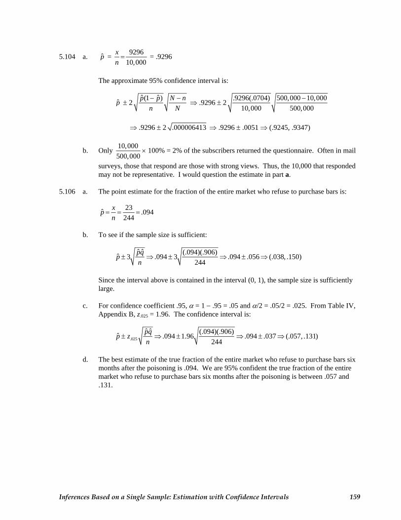
5.104 a. p̂ = 929610,000

x n= = .9296

The approximate 95% confidence interval is:

p̂ ± 2ˆ ˆ(1 )p p N n

n N− − ⇒ .9296 ± 2 .9296(.0704) 500,000 10,000

10,000 500,000 −

⇒ .9296 ± 2 .000006413 ⇒ .9296 ± .0051 ⇒ (.9245, .9347)

b. Only 10,000500,000

× 100% = 2% of the subscribers returned the questionnaire. Often in mail

surveys, those that respond are those with strong views. Thus, the 10,000 that responded may not be representative. I would question the estimate in part a.

5.106 a. The point estimate for the fraction of the entire market who refuse to purchase bars is:

23ˆ .094244

xp n

= = =

b. To see if the sample size is sufficient:

ˆ ˆ (.094)(.906)ˆ 3 .094 3 .094 .056 (.038, .150)

244pqp n

± ⇒ ± ⇒ ± ⇒

Since the interval above is contained in the interval (0, 1), the sample size is sufficiently

large. c. For confidence coefficient .95, α = 1 − .95 = .05 and α/2 = .05/2 = .025. From Table IV,


.025ˆ ˆ (.094)(.906)ˆ .094 1.96 .094 .037 (.057, .131)

244pqp z n

± ⇒ ± ⇒ ± ⇒

d. The best estimate of the true fraction of the entire market who refuse to purchase bars six

months after the poisoning is .094. We are 95% confident the true fraction of the entire market who refuse to purchase bars six months after the poisoning is between .057 and .131.


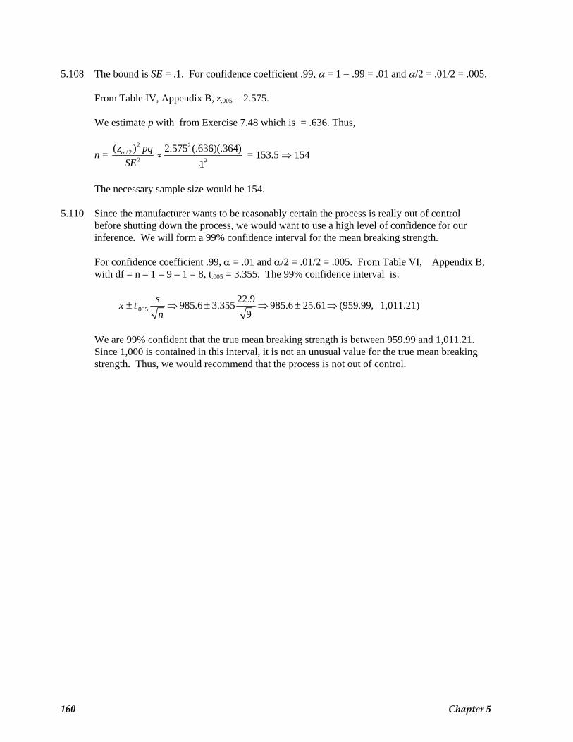
5.108 The bound is SE = .1. For confidence coefficient .99, α = 1 − .99 = .01 and α/2 = .01/2 = .005.

From Table IV, Appendix B, z.005 = 2.575. We estimate p with from Exercise 7.48 which is = .636. Thus,

n = 2 2

/ 22 2

( ) 2.575 (.636)(.364).1

z pq SE

α ≈ = 153.5 ⇒ 154

The necessary sample size would be 154. 5.110 Since the manufacturer wants to be reasonably certain the process is really out of control before shutting down the process, we would want to use a high level of confidence for our inference. We will form a 99% confidence interval for the mean breaking strength. For confidence coefficient .99, α = .01 and α/2 = .01/2 = .005. From Table VI, Appendix B,

with df = n – 1 = 9 – 1 = 8, t.005 = 3.355. The 99% confidence interval is:

.00522.9985.6 3.355 985.6 25.61 (959.99, 1,011.21)

9sx tn

± ⇒ ± ⇒ ± ⇒

We are 99% confident that the true mean breaking strength is between 959.99 and 1,011.21. Since 1,000 is contained in this interval, it is not an unusual value for the true mean breaking strength. Thus, we would recommend that the process is not out of control.

160 Chapter 5

Documents

Arrhythmia Care Co-ordinator Services - NHS Alliance 2012