1

A Direct Monte Carlo Approach for Bayesian Analysis of the Seemingly

Unrelated Regression Model

Arnold Zellner Tomohiro Ando (Chicago GSB)

Theodore W. Anderson’s 90th Birthday Conference, Stanford U.

2

Outline

Background, Motivation

Bayesian Inference for the Seemingly Unrelated Regression Model Using a Direct Monte Carlo Procedure

Numerical results

Conclusion and future work

3

Outline

Background, Motivation

Bayesian Inference for the Seemingly Unrelated Regression Model Using a Direct Monte Carlo Procedure

Numerical results

Conclusion and future works

4

Background and motivation

5

SUR model: Overview

Introduced by Zellner (1962)

Many studies have contributed to the analysis of SUR models.

Many textbooks and journal papersZellner (1963),Gallant (1975), Rocke (1989), Neudecker and Windmeijer (1991), Mandy and Martins (1993), Kurata (1999), Liu (2002), Ng (2002) and references therein. Zellner (1971), Judge et al. (1988), Greene (2002), Geweke (2005), Lancaster (2004), Rossi, McCulloch and Allenby (2005) and so on.

6

SUR model: Overview Cont. Generalized least squares

Zellner (1962, 1963), GLS, Iterative GLS, finite sample Madansky (1964), Iterative GLS and ML

Bayesian Methods Zellner (1971), et al. , approx. finite sample

posteriors, Stein shrinkage, etc. van der Merwve and Viljoen, (1998), Bayesian MOM

Bayesian Markov Chain Monte Carlo estimation Percy (1992, 1996), Chib and Greenberg (1995), Smith and Kohn (2000) and Rossi et al. (2005))

7

SUR model : Motivation

MCMC methods are rather complicated and involve many decisions

Initial parameter valueChoice of an appropriate proposal densityThe length of the burn in periodCheck for convergence

8

SUR model : Motivation

Several drawbacks of MCMC

Can we estimate the Bayesian SUR model by using a direct Monte Carlo (DMC) procedure?

9

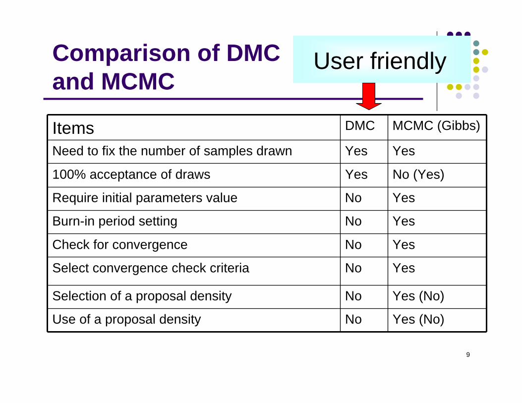
Comparison of DMC and MCMC

Items DMC MCMC (Gibbs)

Need to fix the number of samples drawn Yes Yes

100% acceptance of draws Yes No (Yes)

Require initial parameters value No Yes

Burn-in period setting No Yes

Check for convergence No Yes

Select convergence check criteria No Yes

Selection of a proposal density No Yes (No)

Use of a proposal density No Yes (No)

User friendly

10

Outline

Background, Motivation

Bayesian Inference for the Seemingly Unrelated Regression Model Using a Direct Monte Carlo Procedure

Numerical results

Conclusion and future works

11

The standard SUR models

12

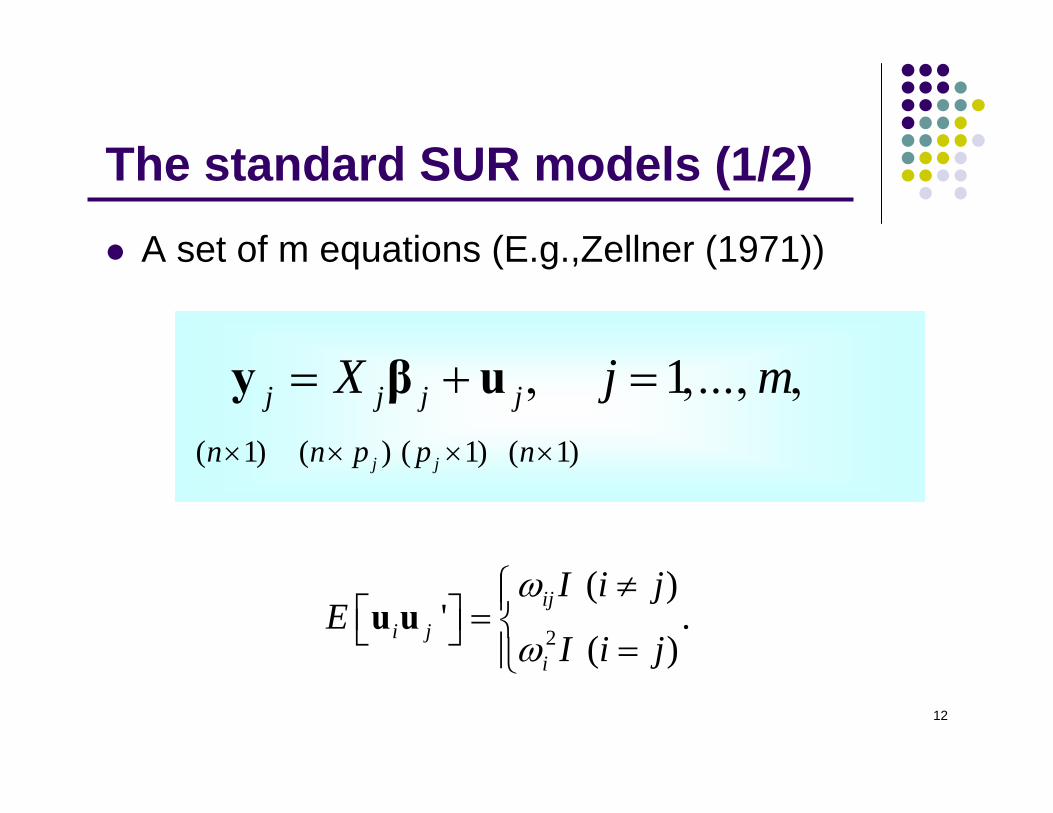
The standard SUR models (1/2)A set of m equations (E.g.,Zellner (1971))

1j j j jX j m= + , = ,..., ,y β u( 1) ( ) ( 1) ( 1)j jn n p p n× × × ×

2

( )' .

( )ij

i ji

I i jE

I i j

ω

ω

≠⎧⎪⎡ ⎤ = ⎨⎣ ⎦ =⎪⎩u u

13

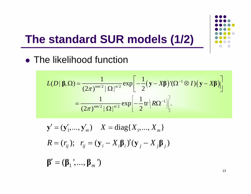
The standard SUR models (1/2)

The likelihood function

1diag{ }mX X X= ,...,1( )m′ ′ ′= ,...,y y y

( ) ( )12 2

12 2

1 1( ) exp '( )(2 ) 2

1 1exp tr(2 ) 2

nm n

nm n

L D X I X

R

π

π

−/ /

⎡ ⎤−⎧ ⎫⎢ ⎥

⎨ ⎬⎢ ⎥/ / ⎩ ⎭⎢ ⎥⎣ ⎦

⎡ ⎤| ,Ω = − − Ω ⊗ −⎢ ⎥| Ω | ⎣ ⎦

= − Ω .| Ω |

β y β y β

( ); ( ) ( )ij ij i i i j j jR r r X X′= = − −y β y β

1( ' ')m′ = ,...,β β β

14

Bayesian estimation

15

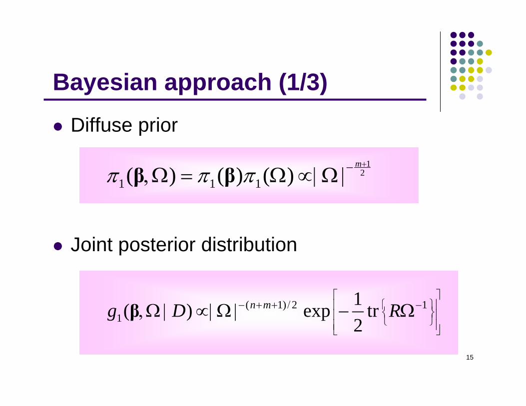
Bayesian approach (1/3)

Diffuse prior

Joint posterior distribution

12

1 1 1( ) ( ) ( )m

π π π+−,Ω = Ω ∝|Ω |β β

( 1) 2 11

1( ) exp tr2

n mg D R⎡ ⎤

− + + / −⎧ ⎫⎢ ⎥⎨ ⎬⎢ ⎥⎩ ⎭⎢ ⎥⎣ ⎦

,Ω | ∝| Ω | − Ωβ

16

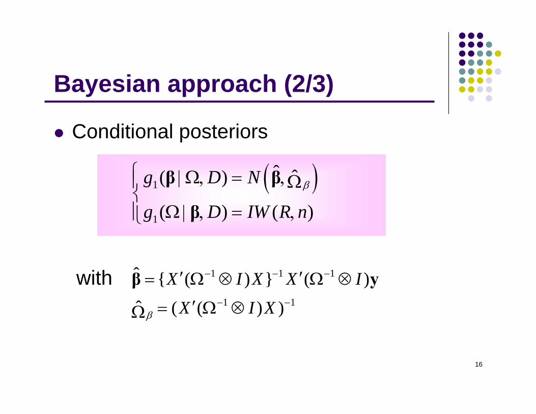
Bayesian approach (2/3)

Conditional posteriors

with

( )1

1

ˆ ˆ( )

( ) ( )

g D N

g D IW R nβ

⎧ | Ω, = ,⎪ Ω⎨

Ω | , = ,⎪⎩

β β

β

1 1 1

1 1

ˆ { ( ) } ( )ˆ ( ( ) )

X I X X IX I Xβ

− − −

− −

′ ′= Ω ⊗ Ω ⊗

′= Ω ⊗Ω

β y

17

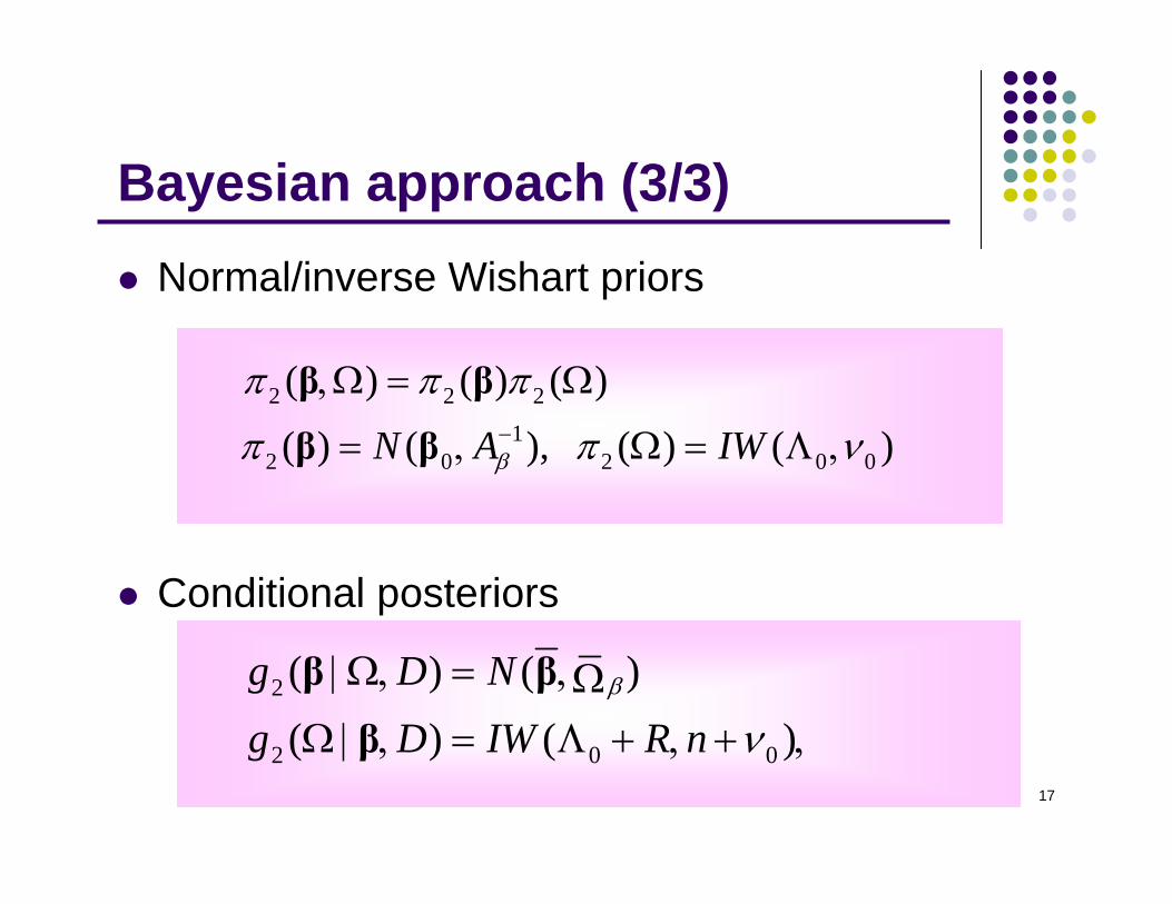
Bayesian approach (3/3)Normal/inverse Wishart priors

Conditional posteriors

2 2 21

2 0 2 0 0

( ) ( ) ( )

( ) ( ), ( ) ( )N A IWβ

π π π

π π ν−

,Ω = Ω

= , Ω = Λ ,

β β

β β

2

2 0 0

( ) ( )( ) ( )

g D Ng D IW R n

β

ν| Ω, = ,Ω

Ω | , = Λ + , + ,

β ββ

18

The DMC procedure for the transformed SUR model

19

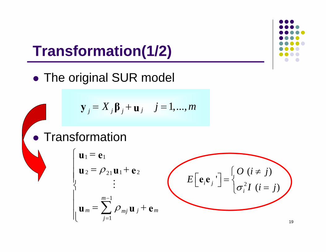
Transformation(1/2)

The original SUR model

Transformation1 1

2 1 221

1

1

m

m j mmjj

ρ

ρ−

=

=⎧⎪ = +⎪⎪⎨⎪⎪ = +⎪⎩

∑

u eu u e

u u e

M

1,...,jjj jX j m= + =y β u

2

( )'

( )i ji

O i jE

I i jσ

≠⎧⎡ ⎤ = ⎨⎣ ⎦ =⎩e e

20

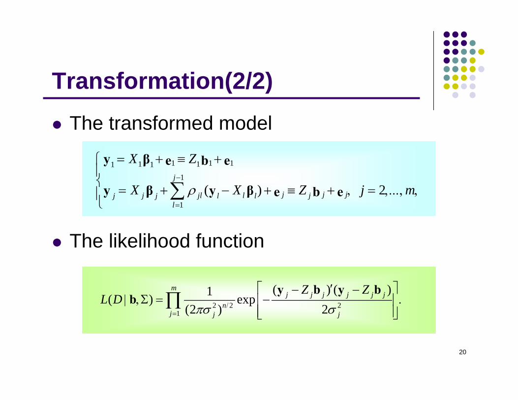
Transformation(2/2)

The transformed model

The likelihood function

1 1 11 11 11

1( ) 2

j

j j jj jl l jj j l ll

X Z

X X Z j mρ−

=

= + ≡ +⎧⎪⎨

= + − + ≡ + , = ,..., ,⎪⎩

∑

y β e b e

y β y β e b e

2 2 21

( ) ( )1( ) exp(2 ) 2

mj j j j j j

nj j j

Z ZL D

πσ σ/=

⎡ ⎤′− −| ,Σ = − .⎢ ⎥

⎢ ⎥⎣ ⎦∏

y b y bb

21

Bayesian estimation

22

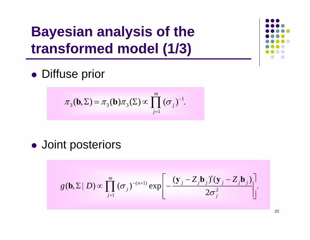
Bayesian analysis of the transformed model (1/3)

Diffuse prior

Joint posteriors

13 3 3

1

( ) ( ) ( ) ( )m

jj

π π π σ −

=

,Σ = Σ ∝ .∏b b

( 1)2

1

( ) ( )( ) ( ) exp

2

mj j j j j jn

jj j

Z Zg D σ

σ− +

=

⎡ ⎤′− −,Σ | ∝ − .⎢ ⎥

⎢ ⎥⎣ ⎦∏

y b y bb

23

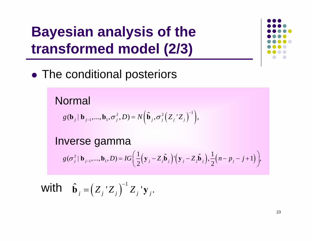
Bayesian analysis of the transformed model (2/3)

The conditional posteriors

with

( )( )12 21 1

ˆ( ,..., , , ) , ' ,j j j j j j jg D N Z Zσ σ−

−| =b b b b

( ) ( ) ( )21 1

1 1ˆ ˆ( ,..., , ) ' , 1 ,2 2j j j j j j j j jg D IG Z Z n p jσ −

⎛ ⎞| = − − − − +⎜ ⎟⎝ ⎠

b b y b y b

( ) 1ˆ ' ' .j j j j jZ Z Z−

=b y

Normal

Inverse gamma

24

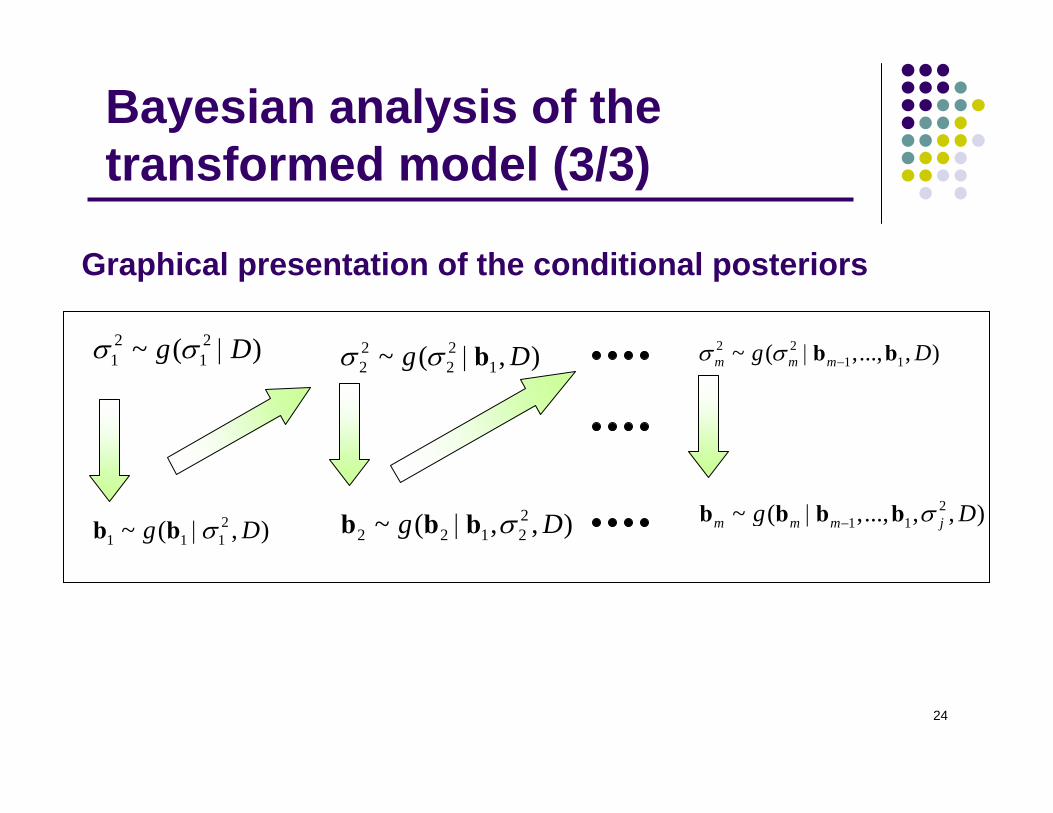
Bayesian analysis of the transformed model (3/3)

21 1 1~ ( , )g Dσ|b b

21 1~ ( ,..., , , )m m m jg Dσ−|b b b b

2 22 2 1~ ( , )g Dσ σ |b

2 21 1~ ( )g Dσ σ | 2 2

1 1~ ( ,..., , )m m mg Dσ σ −|b b

22 2 1 2~ ( , , )g Dσ|b b b

Graphical presentation of the conditional posteriors

25

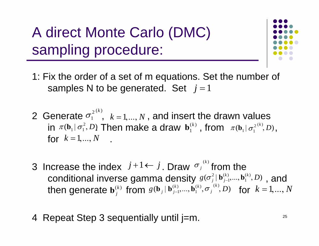
A direct Monte Carlo (DMC) sampling procedure:

1: Fix the order of a set of m equations. Set the number of samples N to be generated. Set

2 Generate , , and insert the drawn valuesin . Then make a draw , from , for .

3 Increase the index . Draw from the conditional inverse gamma density , andthen generate from for

4 Repeat Step 3 sequentially until j=m.

1j =

( )21

kσ 1k N= ,...,2

1 1( )Dπ σ| ,b ( )1kb ( )2

1 1( )k Dπ σ| ,b1k N= ,...,

1j j+ ← ( )kjσ

2 ( ) ( )1 1( )k k

j jg Dσ −| ,..., ,b b( )kjb

( )( ) ( )1 1( )kk k

jj jg Dσ−| , ..., , ,b b b 1k N= ,...,

26

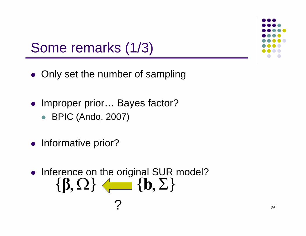
Some remarks (1/3)

Only set the number of sampling

Improper prior… Bayes factor? BPIC (Ando, 2007)

Informative prior?

Inference on the original SUR model?{ } { },Ω ,Σβ b

?

27

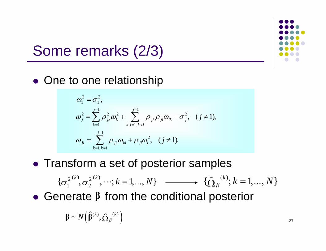
One to one relationship

Transform a set of posterior samples

Generate from the conditional posterior

Some remarks (2/3)

( )ˆ{ 1 }k k Nβ ; = ,...,Ω( ) ( )2 2

1 2{ 1 }k k k Nσ σ, , ; = ,...,L

β

2 21 1

1 12 2 2 2

1 1

12

1

( 1)

( 1)

j j

j jk k jk jl lk jk k l k l

j

ji jk ki ji ik k i

j

j

ω σ

ω ρ ω ρ ρ ω σ

ω ρ ω ρ ω

− −

= , = , <

−

= , ≠

= ,

= + + , ≠ ,

= + , ≠ .

∑ ∑

∑

( )( )( )ˆ ˆ~ kkN β,Ωβ β

28

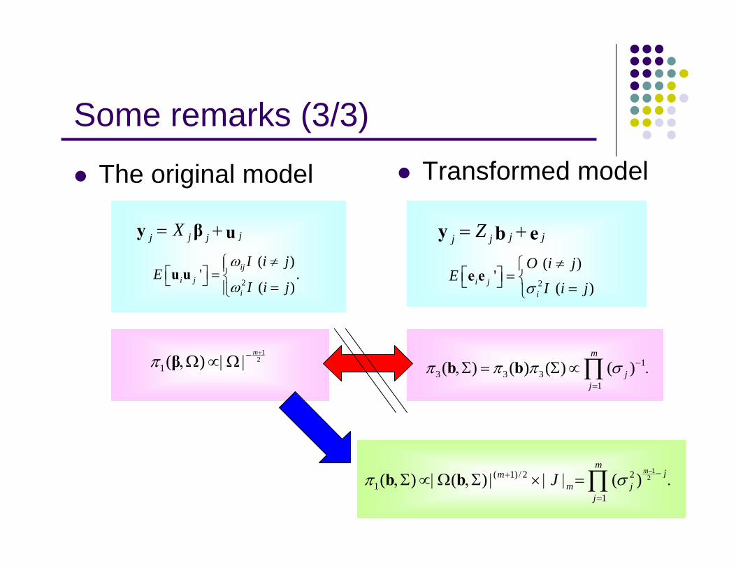
Some remarks (3/3)

The original model

jjj jX= +y β u

2

( )' .

( )ij

i ji

I i jE

I i j

ω

ω

≠⎧⎪⎡ ⎤ = ⎨⎣ ⎦ =⎪⎩u u

12

1( )m

π+−,Ω ∝|Ω |β

Transformed model

j jjj Z= +y b e

2

( )'

( )i ji

O i jE

I i jσ

≠⎧⎡ ⎤ = ⎨⎣ ⎦ =⎩e e

13 3 3

1

( ) ( ) ( ) ( )m

jj

π π π σ −

=

,Σ = Σ ∝ .∏b b

12( 1) 2 2

11

( ) ( ) ( )m

mjm

m jj

Jπ σ− −+ /

=

,Σ ∝| Ω ,Σ | × | | = .∏b b

29

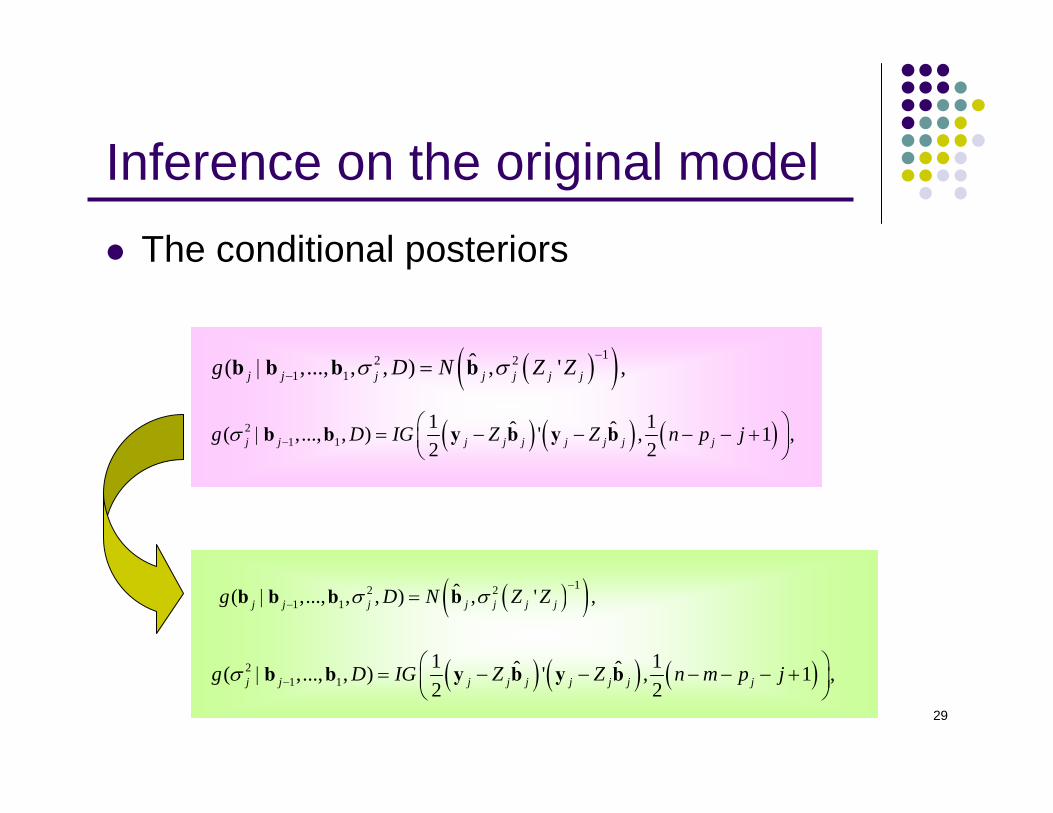
Inference on the original modelThe conditional posteriors

( ) ( ) ( )21 1

1 1ˆ ˆ( ,..., , ) ' , 1 ,2 2j j j j j j j j jg D IG Z Z n m p jσ −

⎛ ⎞| = − − − − − +⎜ ⎟⎝ ⎠

b b y b y b

( )( )12 21 1

ˆ( ,..., , , ) , ' ,j j j j j j jg D N Z Zσ σ−

−| =b b b b

( ) ( ) ( )21 1

1 1ˆ ˆ( ,..., , ) ' , 1 ,2 2j j j j j j j j jg D IG Z Z n p jσ −

⎛ ⎞| = − − − − +⎜ ⎟⎝ ⎠

b b y b y b

( )( )12 21 1

ˆ( ,..., , , ) , ' ,j j j j j j jg D N Z Zσ σ−

−| =b b b b

30

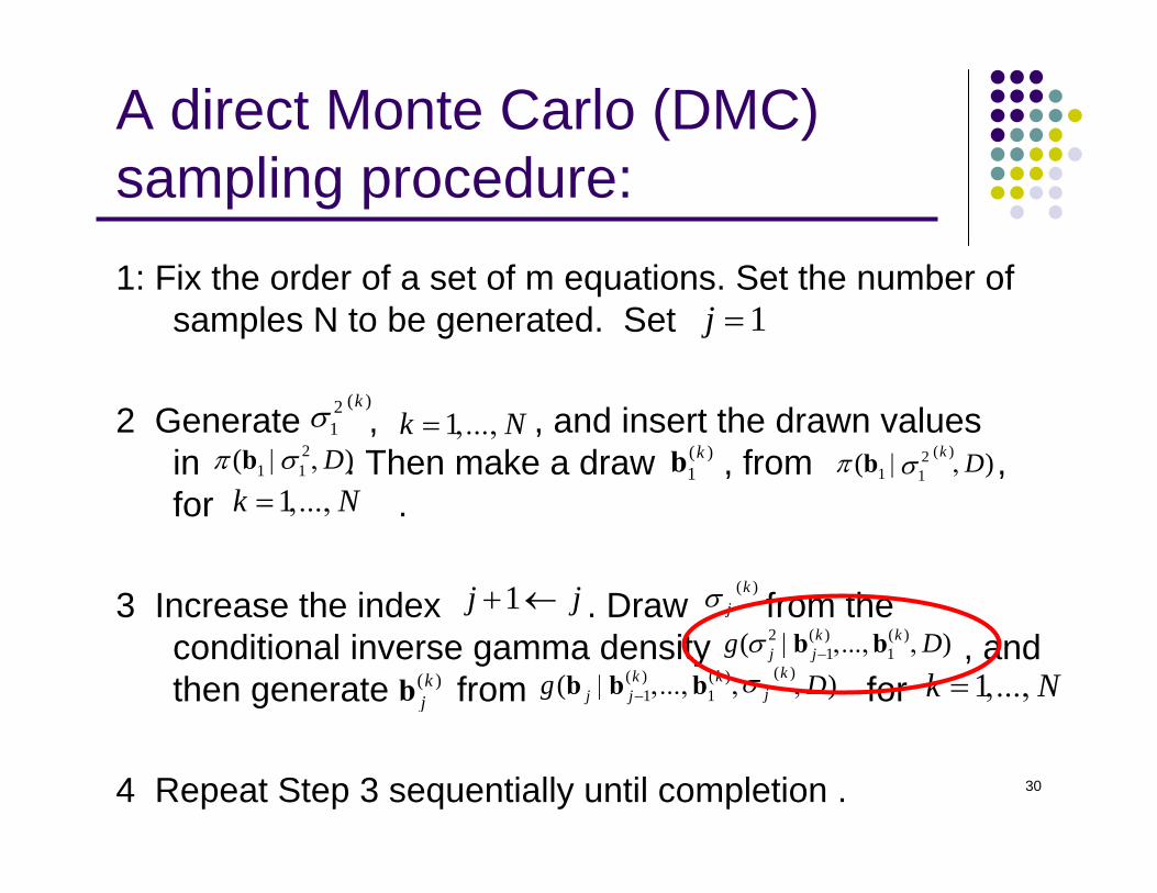
A direct Monte Carlo (DMC) sampling procedure:1: Fix the order of a set of m equations. Set the number of

samples N to be generated. Set

2 Generate , , and insert the drawn valuesin . Then make a draw , from , for .

3 Increase the index . Draw from the conditional inverse gamma density , andthen generate from for

4 Repeat Step 3 sequentially until completion .

1j =

( )21

kσ 1k N= ,...,2

1 1( )Dπ σ| ,b ( )1kb ( )2

1 1( )k Dπ σ| ,b1k N= ,...,

1j j+ ← ( )kjσ

2 ( ) ( )1 1( )k k

j jg Dσ −| ,..., ,b b( )kjb

( )( ) ( )1 1( )kk k

jj jg Dσ−| , ..., , ,b b b 1k N= ,...,

31

Outline

Overview of SUR model

Bayesian Inference for the SUR Model Using a Direct Monte Carlo Procedure

Numerical results

Conclusion and future works

32

Numerical results

33

Simulation study

34

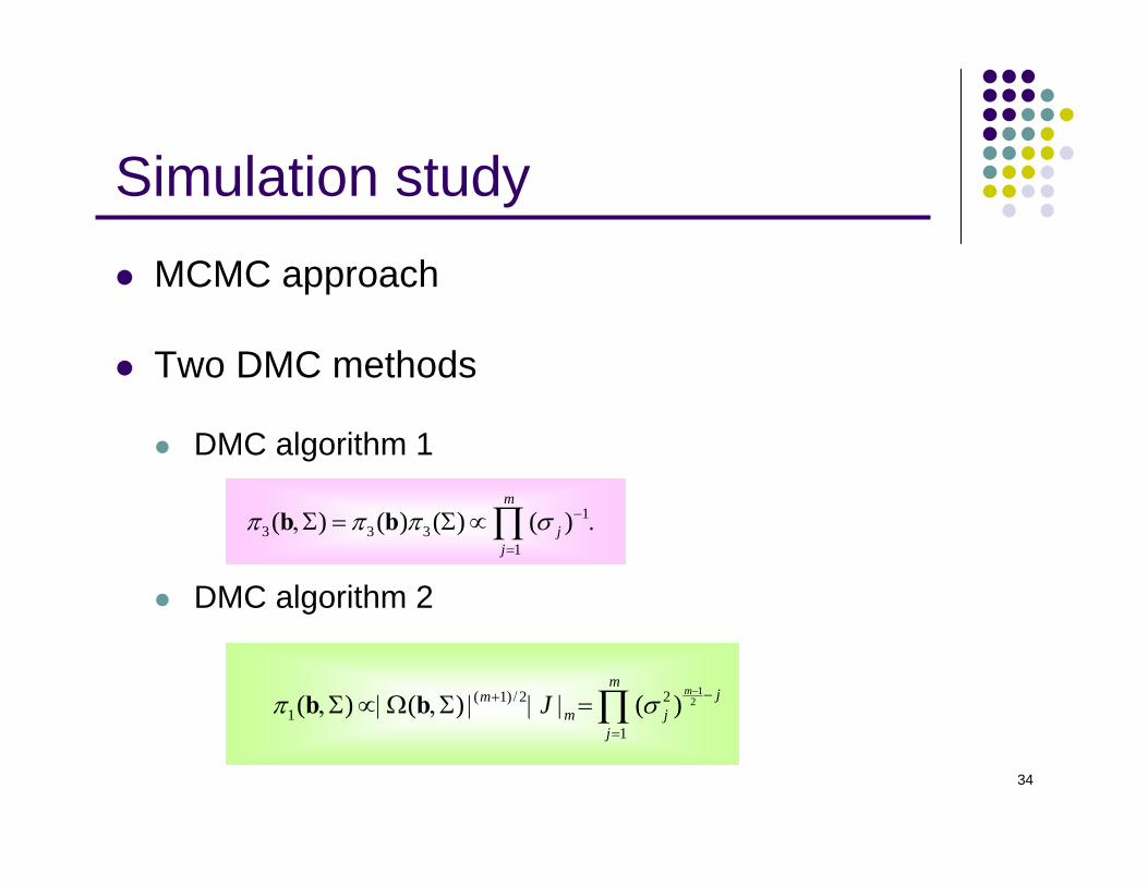
Simulation studyMCMC approach

Two DMC methods

DMC algorithm 1

DMC algorithm 2

13 3 3

1

( ) ( ) ( ) ( )m

jj

π π π σ −

=

,Σ = Σ ∝ .∏b b

12( 1) 2 2

11

( ) ( ) ( )m

mjm

m jj

Jπ σ− −+ /

=

,Σ ∝| Ω ,Σ | | | =∏b b

35

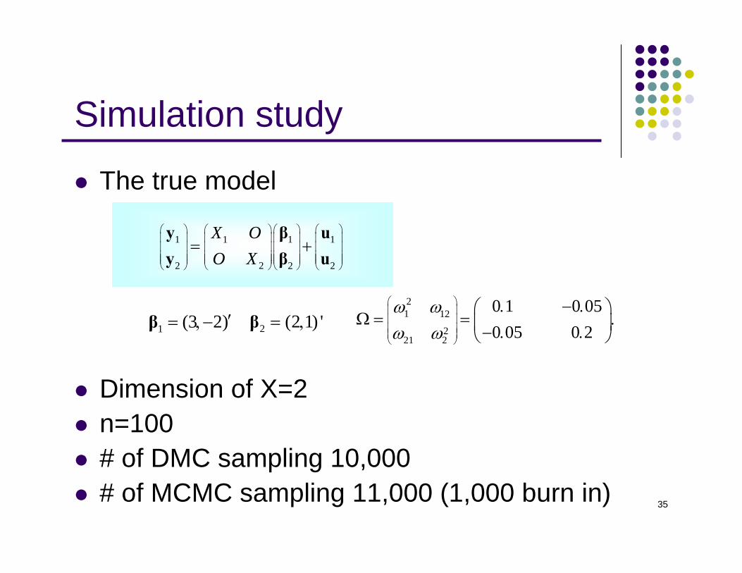
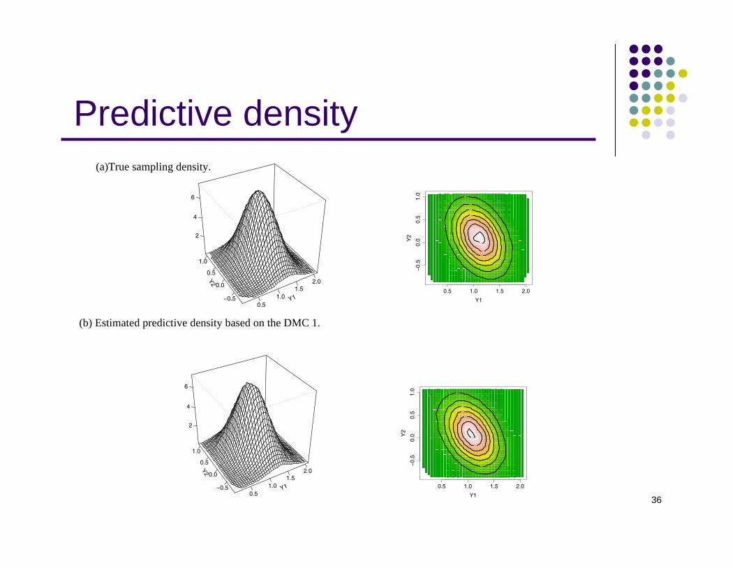
Simulation study

The true model

Dimension of X=2n=100 # of DMC sampling 10,000# of MCMC sampling 11,000 (1,000 burn in)

1 1 11

22 2 2

X OO X

⎛ ⎞ ⎛ ⎞ ⎛ ⎞⎛ ⎞⎜ ⎟ ⎜ ⎟ ⎜ ⎟⎜ ⎟⎜ ⎟ ⎜ ⎟ ⎜ ⎟⎜ ⎟⎜ ⎟ ⎜ ⎟ ⎜ ⎟⎜ ⎟⎜ ⎟⎜ ⎟ ⎜ ⎟ ⎜ ⎟

⎝ ⎠⎝ ⎠ ⎝ ⎠ ⎝ ⎠

= +y β uy β u

21 12

221 2

0 1 0 050 05 0 2

ω ωω ω

⎛ ⎞⎜ ⎟⎜ ⎟⎜ ⎟⎜ ⎟⎝ ⎠

. − .⎛ ⎞Ω = = .⎜ ⎟− . .⎝ ⎠1 (3 2)′= ,−β 2 (2 1) '= ,β

36

Predictive density

Y10.5

1.01.5

2.0Y2

−0.5

0.0

0.5

1.0

2

4

6

0.5 1.0 1.5 2.0

−0.

50.

00.

51.

0

Y1

Y2

Y10.5

1.01.5

2.0Y2

−0.5

0.0

0.5

1.0

2

4

6

0.5 1.0 1.5 2.0

−0.

50.

00.

51.

0

Y1

Y2

(a)True sampling density.

(b) Estimated predictive density based on the DMC 1.

37

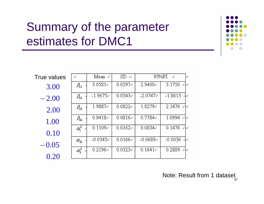
Summary of the parameter estimates for DMC1

3.002.002.001.000.100.050.20

−

−

Note: Result from 1 dataset

True values

38

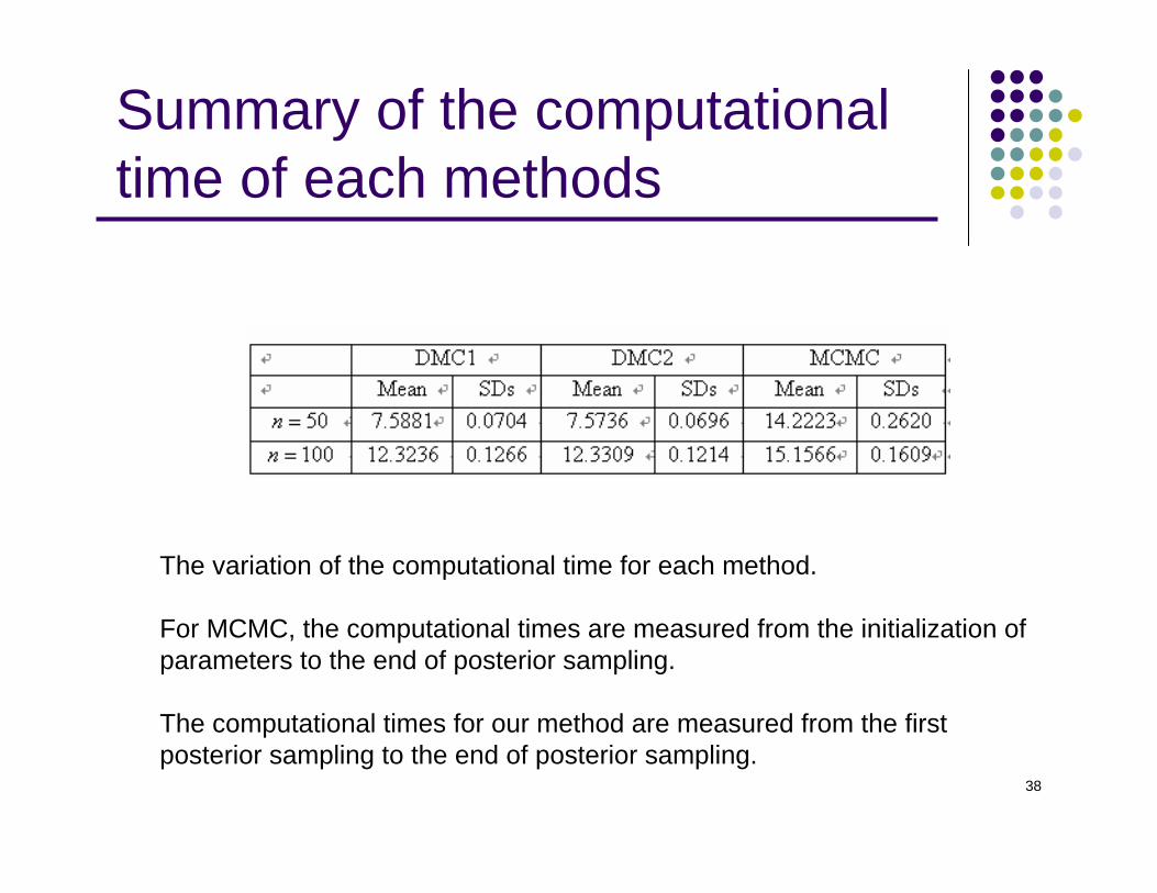
Summary of the computational time of each methods

The variation of the computational time for each method.

For MCMC, the computational times are measured from the initialization of parameters to the end of posterior sampling.

The computational times for our method are measured from the first posterior sampling to the end of posterior sampling.

39

Real data analysis 1

40

Incense product sales forecastIn 2006, the size of the market for incense products in Japan was estimated to be about 30 billion yen.

In Japan, traditional incense is used differently from lifestyle incense.

Data consist of the daily sales figures for incense products from April, 2006 to June, 2006.

The data were collected from two department stores, both located in Tokyo.

41

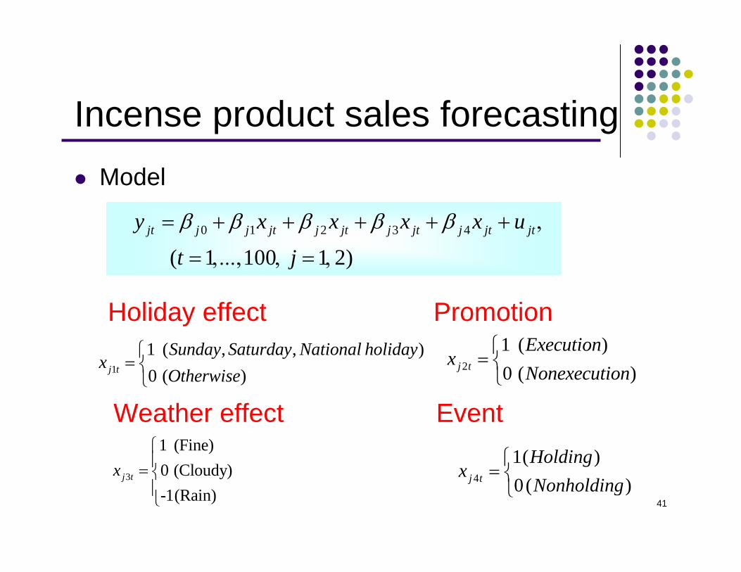
Incense product sales forecastingModel

0 1 2 3 4

( 1 100 1 2)jt j j jt j jt j jt j jt jty x x x x u

t j

β β β β β= + + + + + ,

= ,..., , = ,

1

1 ( , , )0 ( )j t

Sunday Saturday National holidayx

Otherwise⎧

= ⎨⎩

2

1 ( )0 ( )j t

Executionx

Nonexecution⎧

= ⎨⎩

3

1 (Fine)0 (Cloudy)-1(Rain)

j tx⎧⎪= ⎨⎪⎩

4

1( )0( )j t

Holdingx

Nonholding⎧

= ⎨⎩

Holiday effect Promotion

Weather effect Event

42

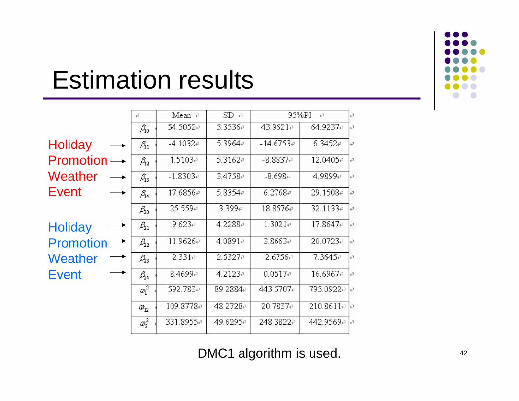
Estimation results

DMC1 algorithm is used.

Holiday PromotionWeather Event

Holiday PromotionWeather Event

43

Real data analysis 2

44

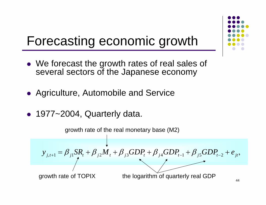
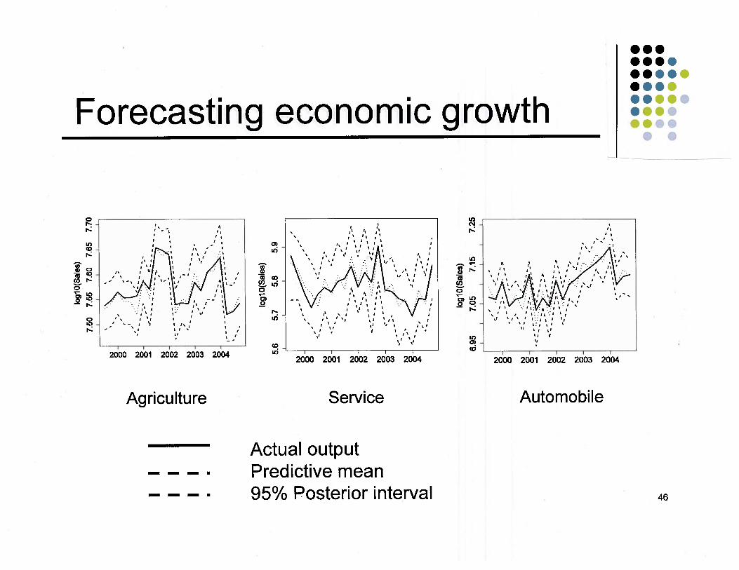
Forecasting economic growthWe forecast the growth rates of real sales of several sectors of the Japanese economy

Agriculture, Automobile and Service

1977~2004, Quarterly data.

1 1 2 3 4 1 5 2j t j t j t j t j t j t jty SR M GDP GDP GDP eβ β β β β, + − −= + + + + + ,

growth rate of TOPIX the logarithm of quarterly real GDP

growth rate of the real monetary base (M2)

45

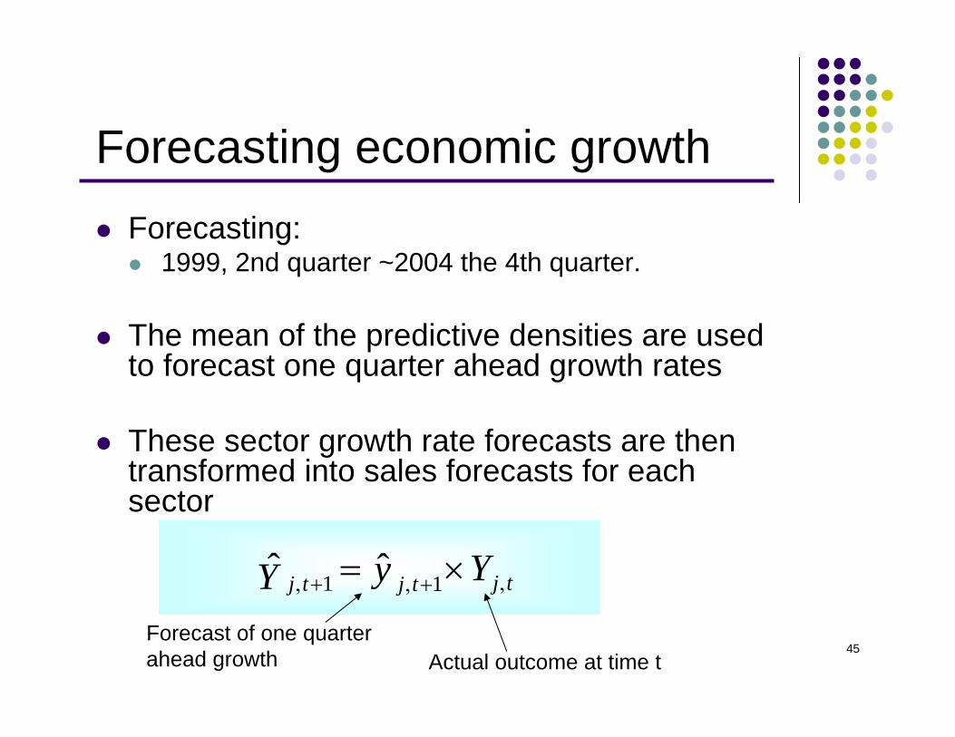
Forecasting economic growthForecasting:

1999, 2nd quarter ~2004 the 4th quarter.

The mean of the predictive densities are used to forecast one quarter ahead growth rates

These sector growth rate forecasts are then transformed into sales forecasts for each sector

1 1ˆ ˆ j tj t j t YyY ,, + , += ×

Actual outcome at time tForecast of one quarter ahead growth

47

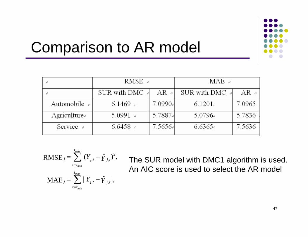
Comparison to AR model

2ˆ( )RMSE

ˆMAE

max

min

max

min

t

j j t j tt t

t

j j t j tt t

Y Y

Y Y

, ,=

, ,=

= − ,

= | − |,

∑

∑

The SUR model with DMC1 algorithm is used.An AIC score is used to select the AR model

48

Outline

Overview of SUR model

Bayesian Inference for the SUR Model Using a Direct Monte Carlo Procedure

Numerical results

Conclusion and future works

49

Conclusion

50

ConclusionA direct Monte Carlo (DMC) approach for Bayesian analysis of SUR models.

Some advantages of DMC

The method performed well in Monte Carlo experiments and applications using actual data.

We can recommend our DMC approach for the analysis and use of the SUR model.

51

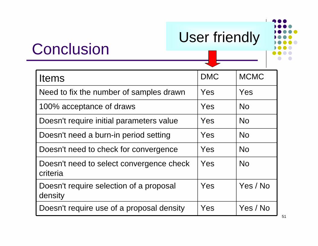
Conclusion

Items DMC MCMC

Need to fix the number of samples drawn Yes Yes

100% acceptance of draws Yes No

Doesn't require initial parameters value Yes No

Doesn't need a burn-in period setting Yes No

Doesn't need to check for convergence Yes No

Doesn't need to select convergence check criteria

Yes No

Doesn't require selection of a proposal density

Yes Yes / No

Doesn't require use of a proposal density Yes Yes / No

User friendly

52

Future workThe DMC approach can be applied to more complex variants of the SUR model, for example those involving use of regression splines, wavelet bases, and so on.

Fat-tailed error.

Numb. of sampling

Our method can be applied to the widely used simultaneous equation model.

Forecasting Japanese economy by MMM model

53

References (1/5)Ando, T. (2007), "Bayesian predictive information criterion for the evaluation of hierarchical Bayesian and empirical Bayes models,'' Biometrika, 94, 443-458.Box, G. E. P. and Tiao, G. C. (1973), Bayesian Inference in Statistical Analysis, Reading, MA: Addison-Wesley. Brooks, SP. and Gelman, A. (1997), "General methods for monitoring convergence of iterative simulations,'' Journal of Computational and Graphical Statistics, 7, 434-455. Carlin, B. and Louis, T. (1996), Bayes and empirical Bayes methods for data analysis, New York: Chapman and Hall. Carroll, R. J., Doug M., Larry F. and Victor K. (2006), "Seemingly unrelated measurement error models, with application to nutritional epidemiology,'' Biometrics, 62, 75-84. Chib, S. and E. Greenberg (1995), "Hierarchical Analysis of SUR Models with Extensions to Correlated Serial Errors and Time-Varying Parameter Models,'' Journal of Econometrics, 68, 339-360. Frasera, D.A.S., Rekkasb, M. and Wong, A. (2005), "Highly accurate likelihood analysis for the seemingly unrelated regression problem,'' Journal of Econometrics, 127, 17-33. Gallant, R. (1975), "Seemingly unrelated nonlinear regressions,'' Journal of Econometrics, 3, 35-50. Gelman, A and Rubin, D.B. (1992), "Inference from iterative simulation using multiple sequences,'' Statistical Science, 7, 457-511.

54

References (2/5)Geweke, J. (1992), "Evaluating the accuracy of sampling-based approaches to calculating posterior moments,'' In Bayesian Statistics 4, eds. J.M. Bernado, J.O. Berger, A.P. Dawid, and A.F.M. Smith, Oxford: Clarendon Press, pp. 169-193. Geweke, J. (2005), Contemporary Bayesian Econometrics and Statistics, New York: Wiley. Greene, W.H. (2002), Econometric Analysis (5th ed.), New Jersey: Prentice-Hall.Gilks, W. R., Richardson, S. and Spiegelhalter, D. J. (1996). Markov Chain Monte Carlo in Practice, New York: Chapman and Hall. Heidelberger P and Welch PD. (1983), "Simulation run length control in the presence of an initial transient,'' Operations Research, 31, 1109-1144. Judge, G., Hill, R., Griffiths, W., Lutkepohl, H., Lee, T. (1988), Introduction to the Theory and Practice of Econometrics. New York: Wiley. Kim, J. K S., Shephard, N. and Chib, S. (1998), "Stochastic volatility likelihood inference and comparison with ARCH models,'' Review of Economic Studies, 65, 361-393. Kowalski, J. R. Mendoza-Blanco, X. M. Tu, and L. J. Gleser (1999), "On the difference ininference and prediction between the joint and independent t-error models for seemingly unrelated regressions,'' Communications in Statistics, Part A - Theory and Methods, 28, 2119-2140. Kurata, H. (1999), "On the efficiencies of several generalized least squares estimators in a seemingly unrelated regression model and a heteroscedastic model,'' Journal of Multivariate Analysis, 70, 86-94.

55

References (3/5)Jeffreys, H. (1946), "An Invariant Form for the Prior Probability in Estimation Problems,'' Proceedings of the Royal Society of London, Series A, 196, 453-461. Jeffreys, H. (1961), Theory of Probability (3rd ed.), Oxford: Oxford University Press. Lancaster T. (2004), Introduction to Modern Bayesian Econometrics, New Jersey: Cambridge University Press.Liu, A. (2002), "Efficient estimation of two seemingly unrelated regression equations,'' Journal of Multivariate Analysis, 82, 445-456. Mandy, D. M. and Martins-Filho, C. (1993), "Seemingly unrelated regressions under additive heteroscedasticity: theory and share equation applications,'' Journal of Econometrics, 58, 315-346. Meyer et al. (2003), "Stochastic volatility: Bayesian computation using automatic differentiation and the extended Kalman filter,'' Econometrics Journal, 6, 408-420.Neudecker, H. and Windmeijer, F. A. G. (1991), " in seemingly unrelated regression equations,'' Statistica Neerlandica, 45, 405-411. Ng, V. M. (2002), "Robust Bayesian Inference for Seemingly Unrelated Regressions with Elliptical Errors,'' Journal of Multivariate Analysis, 83, 409-414. Percy, D. (1992), "Predictions for Seemingly Unrelated Regressions,'' Journal of the Royal Statistical Society B, 54, 243-252. Percy, D.F. (1996), "Zellner's Influence on Multivariate Linear Models,'' in Bayesian Analysis in Statistics and Econometrics: Essays in Honor of Arnold Zellner, eds. D.A. Berry, K.M Chaloner and J.K. Geweke, New York: John Wiley and Sons, pp. 203-214.

56

References (4/5)Press, S. J. (1972), Applied Multivariate Analysis, New York: Holt, Rinehart and Winston, Inc. Raftery, A.E. and Lewis, S.M. (1992), "One long run with diagnostics: Implementation strategies for Markov chain Monte Carlo,'' Statistical Science, 7, 493-497. Rocke, D. M. (1989), "Bootstrap Bartlett adjustment in seemingly unrelated regression,'' Journal of the American Statistical Association, 84, 598-601. Rossi, P.E, Allenby, G. and McCulloch, R. (2005), Bayesian Statistics and Marketing, NJ: John Wiley and Sons. Schruben L.W. (1982), "Detecting initialization bias in simulation experiments,'' Operations Research, 30, 569-590. Smith, M. and R. Kohn, (2000), "Nonparametric Seemingly Unrelated Regression,'' Journal of Econometrics, 98, 257-282. Spiegelhalter, D.J., Best, N.G., Carlin, B.P. and van der Linde, A. (2002), "Bayesian measures of model complexity and fit (with discussion),'' Journal of the Royal Statistical Society, Series B, 64, 583-639.Srivastava, V. K. and Giles, D. E. A. (1987), Seemingly Unrelated Regression Equations Models, New York: Dekker. Tierney, L. (1994), "Markov chains for exploring posterior distributions (with discussion),'' Annals of Statistics, 22, 1701-1762. van der Merwe, A., Viljoen, C. (1988), "Bayesian analysis of the seemingly unrelated regression model,'' Manuscript, University of the Free State, Department of Mathematical Statistics.

57

References (5/5)Zellner, A. (1962), "An efficient method of estimating seemingly unrelated regression equations and tests for aggregation bias,'' Journal of the American Statistical Association, 57, 348-368. Zellner, A. (1963), "Estimators for seemingly unrelated regression equations: some exact finite sample results,'' Journal of the American Statistical Association, 58, 977-992. Zellner, A. (1971), An introduction to Bayesian inference in econometrics, New York : Wiley. Zellner, A. Bauwens, L. and Van Dijk, H. K. (1988), "Bayesian specification analysis and estimation of simultaneous equation models using Monte Carlo Methods,'' Journal of Econometrics, 38, 39-72. Zellner, A. and Chen, B, (2002), "Bayesian Modeling of Economies and Data Requirements,'' Macroeconomic Dynamics, 5, 673-700.Zellner, A. and Min, C.K. (1995), "Gibbs Sampler Convergence Criteria,'' Journal of the American Statistical Association, 90, 921-927.

58

Appendix

59

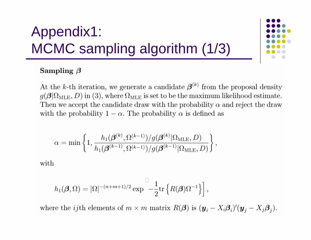
Appendix1: MCMC sampling algorithm (1/3)

60

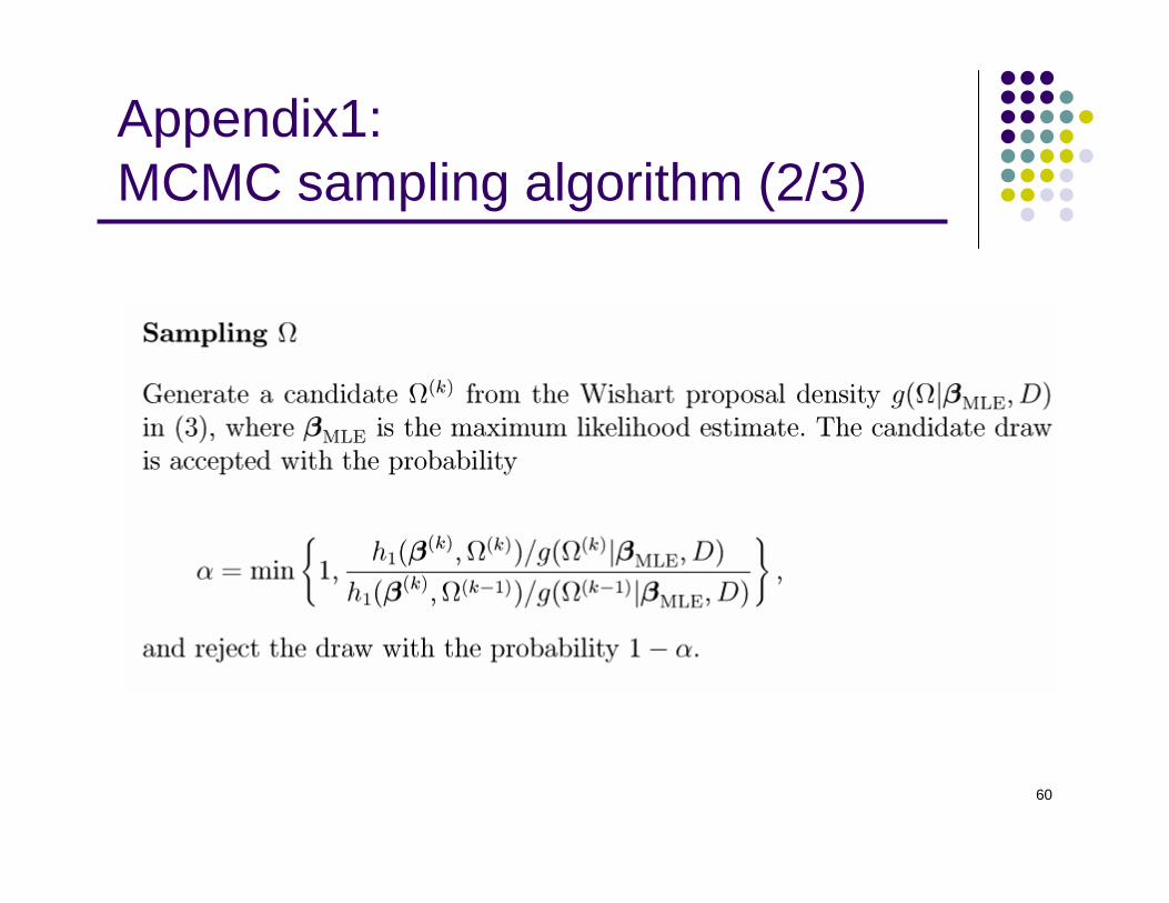
Appendix1: MCMC sampling algorithm (2/3)

61

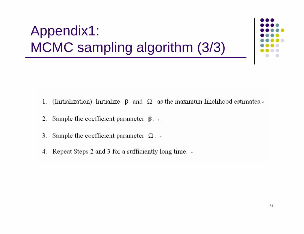
Appendix1: MCMC sampling algorithm (3/3)

62

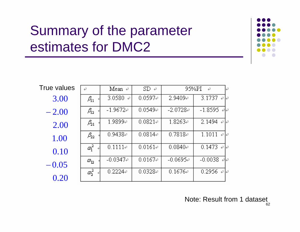
Summary of the parameter estimates for DMC2

3.002.002.001.000.100.050.20

−

−

True values

Note: Result from 1 dataset

63

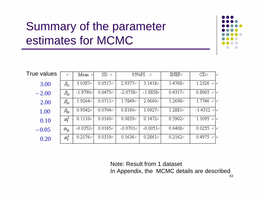
Summary of the parameter estimates for MCMC

3.002.002.001.000.100.050.20

−

−

True values

Note: Result from 1 datasetIn Appendix, the MCMC details are described

64

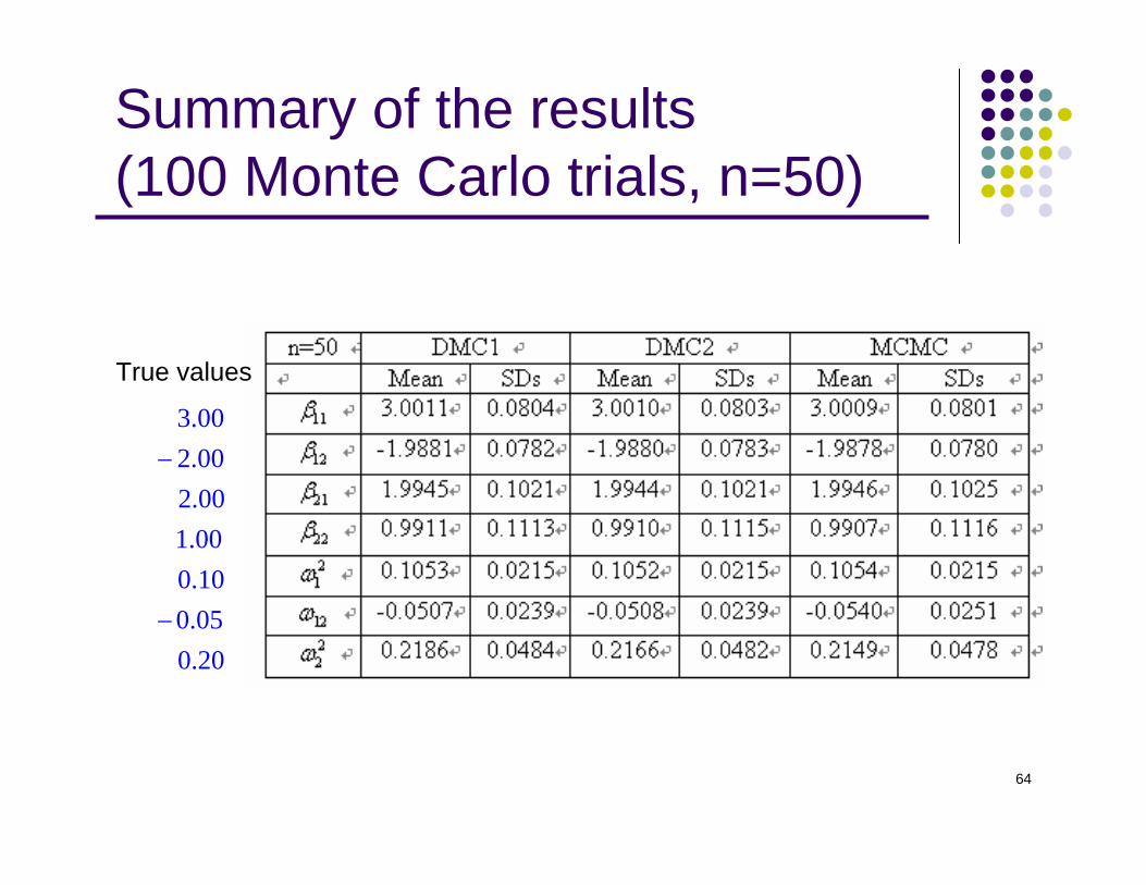
Summary of the results (100 Monte Carlo trials, n=50)

3.002.002.001.000.100.050.20

−

−

True values

65

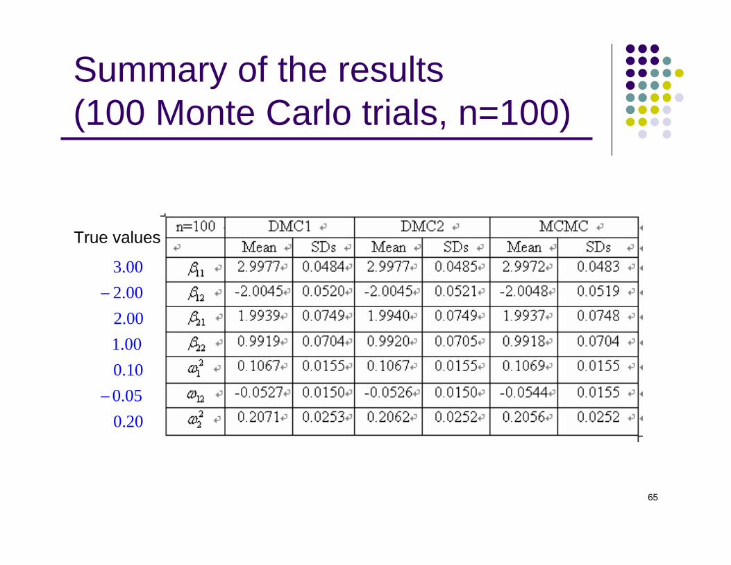
Summary of the results (100 Monte Carlo trials, n=100)

3.002.002.001.000.100.050.20

−

−

True values

66

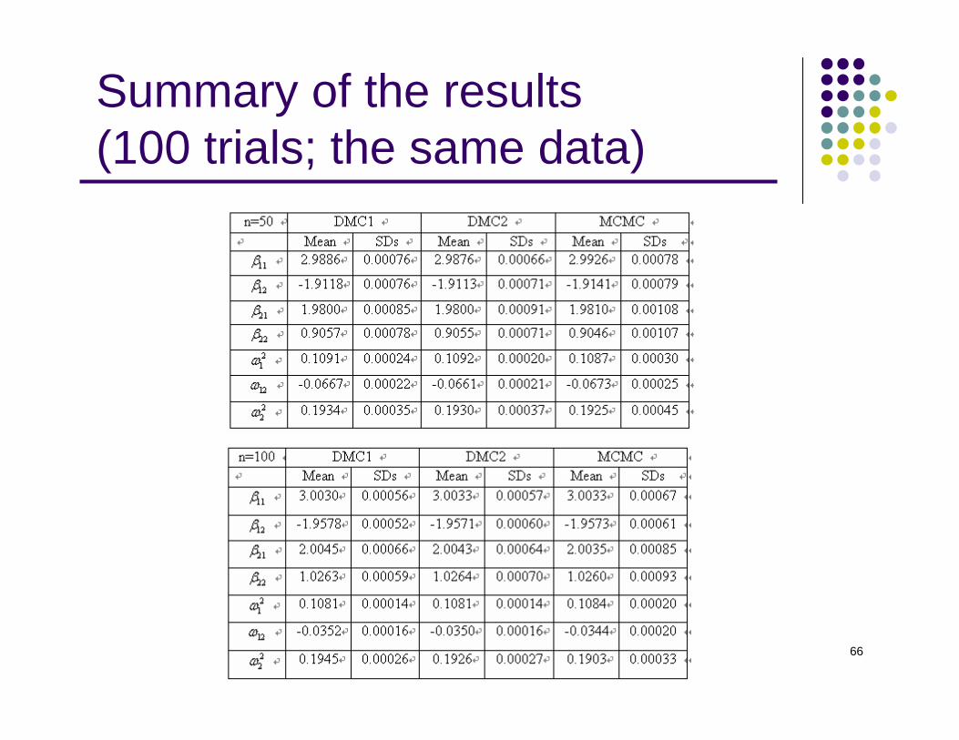
Summary of the results (100 trials; the same data)

67

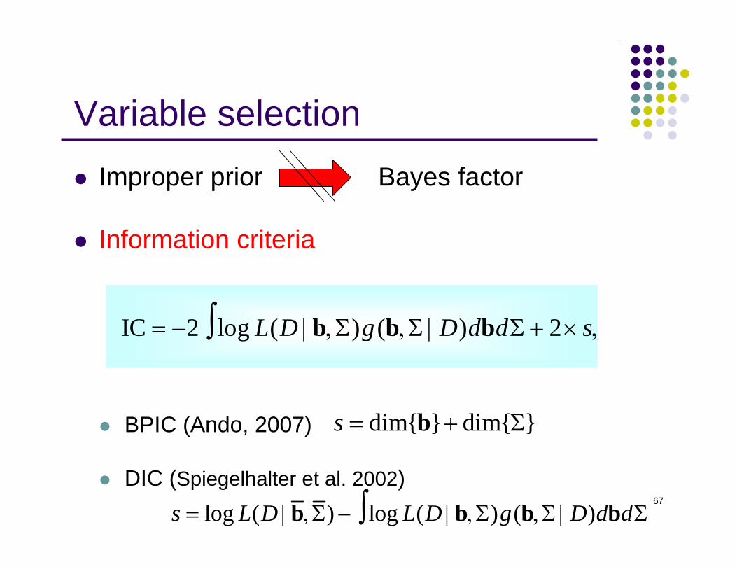
Variable selection

IC 2 log ( ) ( ) 2L D g D d d s= − | ,Σ ,Σ | Σ + × ,∫ b b b

Improper prior Bayes factor

Information criteria

BPIC (Ando, 2007)

DIC (Spiegelhalter et al. 2002)log ( ) log ( ) ( )s L D L D g D d d= | ,Σ − | ,Σ ,Σ | Σ∫b b b b

dim{ } dim{ }s = + Σb

68

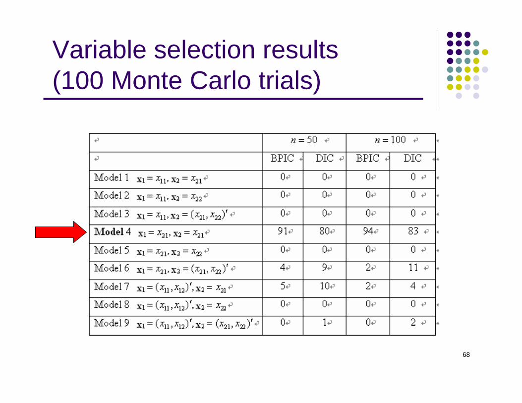
Variable selection results (100 Monte Carlo trials)

69

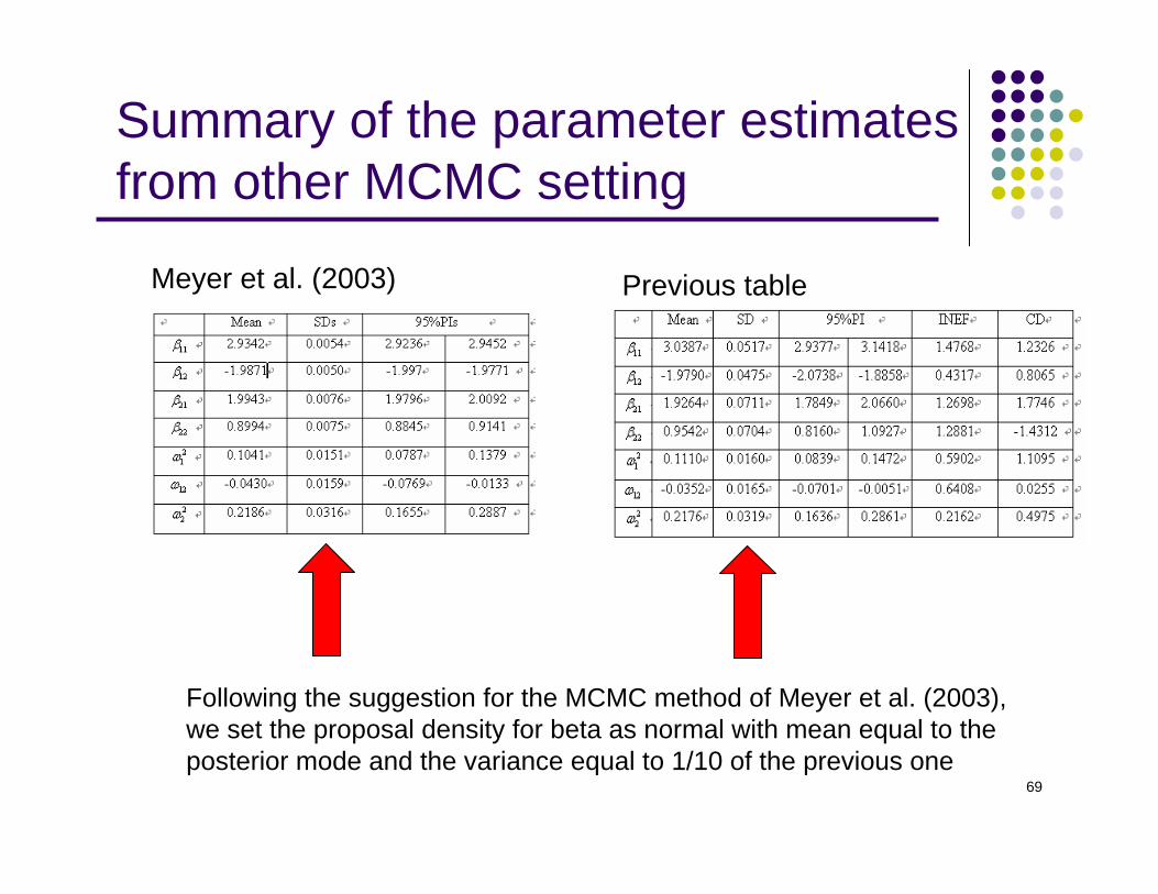
Summary of the parameter estimates from other MCMC setting

Following the suggestion for the MCMC method of Meyer et al. (2003), we set the proposal density for beta as normal with mean equal to the posterior mode and the variance equal to 1/10 of the previous one

Meyer et al. (2003) Previous table

70