Arnold, T., Manning, A. J., Kim, J., Li, S., Webster, H., Thomson, D.,Mühle, J., Weiss, R. F., Park, S., & O'Doherty, S. (2018). Inversemodelling of CF4 and NF3 emissions in East Asia. AtmosphericChemistry and Physics, 18(18), 13305-13320.https://doi.org/10.5194/acp-18-13305-2018

Publisher's PDF, also known as Version of recordLicense (if available):CC BYLink to published version (if available):10.5194/acp-18-13305-2018

Link to publication record in Explore Bristol ResearchPDF-document

This is the final published version of the article (version of record). It first appeared online via EGU at DOI:10.5194/acp-18-13305-2018. Please refer to any applicable terms of use of the publisher.

University of Bristol - Explore Bristol ResearchGeneral rights

This document is made available in accordance with publisher policies. Please cite only thepublished version using the reference above. Full terms of use are available:http://www.bristol.ac.uk/red/research-policy/pure/user-guides/ebr-terms/

Atmos. Chem. Phys., 18, 13305–13320, 2018https://doi.org/10.5194/acp-18-13305-2018© Author(s) 2018. This work is distributed underthe Creative Commons Attribution 4.0 License.

Inverse modelling of CF4 and NF3 emissions in East AsiaTim Arnold1,2,3, Alistair J. Manning3, Jooil Kim4, Shanlan Li5, Helen Webster3, David Thomson3, Jens Mühle4,Ray F. Weiss4, Sunyoung Park5,6, and Simon O’Doherty7

1National Physical Laboratory, Teddington, Middlesex, UK2School of GeoSciences, University of Edinburgh, Edinburgh, UK3Met Office, Exeter, UK4Scripps Institution of Oceanography, University of California, San Diego, CA, USA5Kyungpook Institute of Oceanography, Kyungpook National University, Daegu, South Korea6Department of Oceanography, Kyungpook National University, Daegu, South Korea7School of Chemistry, University of Bristol, Bristol, UK

Correspondence: Tim Arnold (tim.arnold@ed.ac.uk)

Received: 13 December 2017 – Discussion started: 12 February 2018Revised: 18 July 2018 – Accepted: 7 August 2018 – Published: 17 September 2018

Abstract. Decadal trends in the atmospheric abundancesof carbon tetrafluoride (CF4) and nitrogen trifluoride (NF3)have been well characterised and have provided a time se-ries of global total emissions. Information on locations ofemissions contributing to the global total, however, is cur-rently poor. We use a unique set of measurements between2008 and 2015 from the Gosan station, Jeju Island, SouthKorea (part of the Advanced Global Atmospheric Gases Ex-periment network), together with an atmospheric transportmodel, to make spatially disaggregated emission estimatesof these gases in East Asia. Due to the poor availabilityof good prior information for this study, our emission es-timates are largely influenced by the atmospheric measure-ments. Notably, we are able to highlight emission hotspotsof NF3 and CF4 in South Korea due to the measurementlocation. We calculate emissions of CF4 to be quite con-stant between the years 2008 and 2015 for both China andSouth Korea, with 2015 emissions calculated at 4.3± 2.7and 0.36±0.11 Gg yr−1, respectively. Emission estimates ofNF3 from South Korea could be made with relatively smalluncertainty at 0.6± 0.07 Gg yr−1 in 2015, which equates to∼ 1.6 % of the country’s CO2 emissions. We also apply ourmethod to calculate emissions of CHF3 (HFC-23) between2008 and 2012, for which our results find good agreementwith other studies and which helps support our choice inmethodology for CF4 and NF3.

1 Introduction

The major greenhouse gases (GHGs) – carbon dioxide,methane, and nitrous oxide – have natural and anthropogenicsources. The synthetic fluorinated species – chlorofluoro-carbons (CFCs), hydrochlorofluorocarbons (HCFCs), hy-drofluorocarbons (HFCs), and perfluorocarbons (PFCs), sul-fur hexafluoride (SF6) and nitrogen trifluoride (NF3) – are al-most or entirely anthropogenic and are released from indus-trial and domestic appliances and applications. Of the syn-thetic species, tetrafluoromethane (CF4) and NF3 are emit-ted nearly exclusively from point sources of specialised in-dustries (Arnold et al., 2013; Mühle et al., 2010, Worton etal., 2007). Although these species currently make up only asmall percentage of current emissions contributing to globalradiative forcing, they have potential to form large portionsof specific company, sector, state, province, or even countrylevel GHG budgets.

CF4 is the longest-lived GHG known, with an estimatedlifetime of 50 000 years, leading to a global warming po-tential on a 100-year timescale (GWP100) of 6630 (Myhreet al., 2013). Significant increases in atmospheric concen-trations are ascribed mainly to emissions from primary alu-minum production during so-called “anode events” whenthe alumina feed to the reduction cell is restricted (Interna-tional Aluminium Institute, 2016), and from the microchip-manufacturing component of the semiconductor industry (Il-luzzi and Thewissen, 2010). Recently, evidence emerged

Published by Copernicus Publications on behalf of the European Geosciences Union.

13306 T. Arnold et al.: Inverse modelling of CF4 and NF3 emissions

that, similar to primary aluminium production, rare earth el-ement production may also release substantial amounts ofCF4 (Vogel et al., 2017; Zhang et al., 2017). Other emis-sion sources for CF4 include release during the productionof SF6 and HCFC-22, but emissions from these sources areestimated to be small compared to the emissions from thealuminium production and semiconductor manufacturing in-dustries (EC-JRC/PBL, 2013; Mühle et al., 2010). There isalso a very small natural emission source of CF4, sufficientto maintain the pre-industrial atmospheric burden (Deeds etal., 2008; Worton et al., 2007).

According to the Intergovernmental Panel on ClimateChange (IPCC) fifth assessment, NF3’s global warming po-tential on a 100-year timescale (GWP100) is ∼ 16100 (basedon an atmospheric lifetime of 500 years) (Myhre et al.,2013); however, recent work suggests the GWP100 is higherat 19 700 due to an increased estimate in the radiative effi-ciency (Totterdill et al., 2016). Use of NF3 began in the 1960sin specialty applications, e.g. as a rocket fuel oxidiser andas a fluorine donor for chemical lasers (Bronfin and Hazlett,1966). Beginning in the late 1990s, NF3 has been used bythe semiconductor industry, and in the production of pho-tovoltaic cells and flat-panel displays. NF3 can be brokendown into reactive fluorine (F) radicals and ions, which areused to remove the remaining silicon-containing deposits inprocess chambers (Henderson and Woytek, 1994; Johnson etal., 2000). NF3 was also chosen because of its promise asan environmentally friendly alternative, with conversion effi-ciencies to create reactive F far higher than other compoundssuch as C2F6 (Johnson et al., 2000; International SEMAT-ECH Manufacturing Initiative, 2005). Given its rapid recentrise in the global atmosphere and projected future market, ithas been estimated that NF3 could become the fastest grow-ing contributor to radiative forcing of all the synthetic GHGsby 2050 (Rigby et al., 2014).

CF4 and NF3 are not the only species with major pointsource emissions. Trifluoromethane (CHF3; HFC-23) is prin-cipally made as a byproduct in the production of chlorodi-fluoromethane (CHClF2, HCFC-22). Of the HFCs, HFC-23has the highest 100-year global warming potential (GWP100)at 12 400, most significantly due to a long atmospheric life-time of 222 years (Myhre et al., 2013). Its regional and globalemissions have been the subject of numerous previous stud-ies (Fang et al., 2014, 2015; McCulloch and Lindley, 2007;Miller et al., 2010; Montzka et al., 2010; Stohl et al., 2010;Li et al., 2011; Kim et al., 2010; Yao et al., 2012; Kelleret al., 2012; Yokouchi et al., 2006; Simmonds et al., 2018).Thus, emissions of HFC-23 are already relatively well char-acterised from a bottom-up and a top-down perspective. Inthis work, we will also calculate HFC-23 emissions, not toadd to current knowledge, but to provide a level of confi-dence for our methodology.

Unlike for HFC-23, the spatial distribution of emissionsresponsible for CF4 and NF3 abundances is very poorlyunderstood, which is hindering action for targeting mitiga-

tion. HFC-23 is emitted from well-known sources (namelyHCFC-22 production sites) with well-characterised estimatesof emission magnitudes, and hence it has been a targetfor successful mitigation (by thermal destruction) via theclean development mechanism (Miller et al., 2010). How-ever, emissions of CF4 and NF3 are very difficult to estimatefrom industry level information: emissions from Al produc-tion are highly variable depending on the conditions of man-ufacturing, and emissions from the electronics industry de-pend on what is being manufactured, the company’s recipesfor production (such information is not publicly available),and whether abatement methods are used and how efficientthese are under real conditions. Both the Al production andsemiconductor industries have launched voluntary efforts tocontrol their emissions of these substances, reporting suc-cess in meeting their goals (International Aluminium Insti-tute, 2016; Illuzzi and Thewissen, 2010; World Semiconduc-tor Council, 2017). Despite the industry’s efforts to reduceemissions, top-down studies on the emissions of CF4 andNF3 have shown the bottom-up inventories are likely to behighly inaccurate. Most recently, Kim et al. (2014) showedthat global bottom-up estimates for CF4 are as much as 50 %lower than top-down estimates, and Arnold et al. (2013)showed that the best estimates of global NF3 emissions cal-culated from industry information and statistical data totalonly ∼ 35 % of those estimated from atmospheric measure-ments.

Accurate emission estimates of NF3 and CF4 are difficultto make based on simple parameters such as integrated coun-try level uptake rates and leakage rates, which, for example,underpin calculations of HFC emissions. Active or passiveactivities to reduce emissions vary between countries, andbetween industries and companies within countries, and theimpetus to accurately understand emissions is lacking in re-gions that have not been required to report emissions un-der the United Nations Framework Convention on ClimateChange (UNFCCC). This problem is compounded by thedifficulty in making measurements of these gases: CF4 andNF3 are the two most volatile GHGs after methane, and havevery low atmospheric abundances, which makes routine mea-surements in the field at the required precision particularlydifficult. The Advanced Global Atmospheric Gases Experi-ment (AGAGE) has been monitoring the global atmospherictrace gas budget for decades (Prinn et al., 2018). Most re-cently, AGAGE’s “Medusa” preconcentration GC-MS (gaschromatography–mass spectrometry) system has been ableto measure a full suite of the long-lived halogenated GHGs(Arnold et al., 2012; Miller et al., 2008). The Medusa is theonly instrument demonstrated to measure NF3 in ambient airsamples and the only field-deployable instrument capable ofmeasuring CF4. The Medusa on Jeju Island, South Korea,is one of only 20 such instruments currently in operationglobally and is uniquely sensitive to the dominant emissionsources of these compounds given its location in this highlyindustrial part of the globe with large capacities of Al produc-

Atmos. Chem. Phys., 18, 13305–13320, 2018 www.atmos-chem-phys.net/18/13305/2018/

T. Arnold et al.: Inverse modelling of CF4 and NF3 emissions 13307

tion, semiconductor manufacturing, and rare Earth elementproduction industries. Its utility has already been demon-strated in numerous previous studies to understand emissionsof many GHGs from Japan, South Korea, North Korea, east-ern China, and surrounding countries (Fang et al., 2015; Kimet al., 2010; Li et al., 2011).

For the first time, we use the measurements of CF4 (start-ing in 2008) and NF3 (starting in 2013) in an inversion frame-work – coupling each measurement with an air history mapcomputed using a particle dispersion model. We demonstratethe use of these measurements to find emission hotspots inthis unique region with minimal use of prior information, andwe show that East Asia is a major source of these species. Fo-cussed mitigation efforts, based on these results, could have asignificant impact on reducing GHG emissions from specificareas. The technology for abating emissions of these gasesfrom such discrete sources exists and could be used (Changand Chang, 2006; Purohit and Höglund-Isaksson, 2017; Il-luzzi and Thewissen, 2010; Yang et al., 2009; Raoux, 2007;Wangxing et al., 2016).

2 Methods

2.1 Atmospheric measurements

The Gosan station (from here on termed GSN) is locatedon the south-western tip of Jeju Island in South Korea(33.29244◦ N, 126.16181◦ E). The station rests at the top ofa 72 m cliff, about 100 km south of the Korean Peninsula,500 km north-east of Shanghai, China, and 250 km west ofKyushu, Japan, with an air inlet 17 m above ground level(a.g.l.).

A Medusa GC-MS system was installed at GSN in 2007and has been operated as part of the AGAGE network to takeautomated, high-precision measurements for a wide rangeof CFCs, HCFCs, HFCs, PFCs, Halons, and other halocar-bons, and all significant synthetic GHGs and/or stratosphericozone-depleting gases as well as many naturally occurringhalogenated compounds (Miller et al., 2008; Arnold et al.,2012; Kim et al., 2010). Since November 2013, NF3 hasbeen measured within this suite of gases. Air reaches GSNfrom the most heavily developed areas of East Asia, makingthe measurements and their interpretation a unique source fortop-down emission estimates in the region. Ambient air mea-surements are made every 130 min and are bracketed witha standard before and after the air sample in order to cor-rect for instrumental drift in calibration. Further details onthe methodology for the calibration of these gases are givenelsewhere (Arnold et al., 2012; Mühle et al., 2010; Miller etal., 2010; Prinn et al., 2018).

2.2 Atmospheric model

Lagrangian particle dispersion models are well suited to de-termine emissions of trace gases on this spatial scale as they

can be run backwards, allowing for the source–receptor re-lationship to be efficiently calculated. We use the Numeri-cal Atmospheric dispersion Modelling Environment (NAMEIII), henceforth called NAME, developed by the UK Met Of-fice (Ryall and Maryon, 1998; Jones et al., 2007). Inert parti-cles are advected backwards in time by the transport model,NAME, which also associates a mass to each trajectory.Hence, NAME output is provided as the time-integrated near-surface (0–40 m) air concentration (g s m−3) in each grid cell– the surface influence resulting from a conceptual releaseat a specific rate (g s−1) from the site. “Offline”, this surfaceinfluence is divided by the total mass emitted during the 1 hrelease time and multiplied by the geographical area of eachgrid box to form a new array with each component repre-sentative of how 1 g m−2 s−1 of continuous emissions from agrid square would result in a measured concentration at themodel’s release point (the measurement site). Multiplicationof each grid component by an emission rate then results in acontribution to the concentration.

The meteorological parameter inputs to NAME are fromthe Met Office’s operational global NWP model, the Uni-fied Model (UM) (Cullen, 1993). The UM had a horizon-tal resolution of 0.5625◦×0.375◦ (∼ 40 km) from December2007 to April 2010; 0.3516◦×0.2344◦ (∼ 25 km) from April2010 to July 2014; and 0.234375×0.15625◦ (∼ 17 km) frommid-July 2014 to mid-July 2017. The number of vertical lev-els in the UM has increased over this period, with NAMEtaking the lowest 31 levels in 2009 and the lowest 59 lev-els in 2015. The GHGs considered in this study have life-times on the order of hundreds to tens of thousands of years(Myhre et al., 2013) and can be considered inert gases onthe spatial and temporal scales of this study, and thereforethe NAME model schemes for representing chemistry, drydeposition, wet deposition, and radioactive decay were notused. The planetary boundary layer height (BLH) estimatesare taken from the UM; however, a minimum BLH allowedwithin NAME was set to 40 m to be consistent with the max-imum emission height and the height of the output grid. TheNAME model was run to estimate the 30-day history of theair on the route to GSN. We calculated the time-integratedair concentration (dosage) at each grid box (0.352◦×0.234◦,0–40 m a.g.l., irrespective of the underlying UM meteorologyresolution) from a release of 1 g s−1 at GSN at 17±10 m a.g.l.

The model is three-dimensional, and therefore it is not justsurface-to-surface transport that is modelled: an air parcelcan travel from the surface to a high altitude and then backto the surface, but only those times when the air parcel iswithin the lowest 40 m above the ground will be included inthe model output aggregated sensitivity maps. The computa-tional domain covers 54.34◦ E to 168.028◦W longitude (391grid cells of dimension 0.352◦) and 5.3◦ S to 74.26◦ N lat-itude (340 grid cells of dimension 0.234◦), and extends tomore than 19 km vertically. Despite the increase in the reso-lution of the UM over the time period covered, the resolutionof the NAME output was kept constant throughout. For each

www.atmos-chem-phys.net/18/13305/2018/ Atmos. Chem. Phys., 18, 13305–13320, 2018

13308 T. Arnold et al.: Inverse modelling of CF4 and NF3 emissions

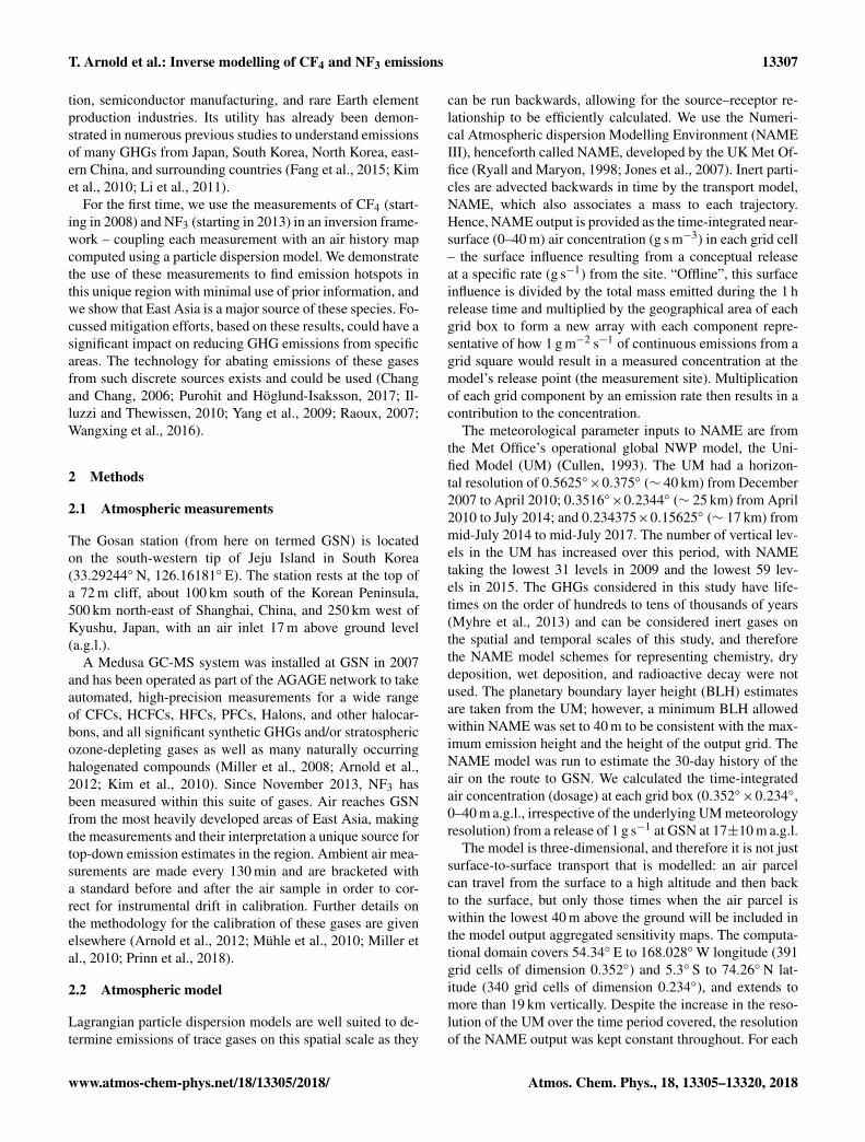
Figure 1. An aggregation of the dilution matrices from 2013, gen-erated using NAME output (see Sect. 2.2), illustrating the relativesensitivity of measurements at GSN to emissions in the region.

1 h period, 5000 inert model particles were used to describethe dispersion of air. By dividing the dosage (g s m−3) by thetotal mass emitted (3600 s h−1

× 1 h× 1 g s−1) and multiply-ing by the geographical area of each grid box (m2), the modeloutput was converted into a dilution matrix H (s m−1). InFig. 1, we show an aggregated dilution matrix for the 2013inversion period, demonstrating the areas of most significantinfluence on the GSN measurements. Each element of thematrix H dilutes a continuous emission of 1 g m−2 s−1 froma given grid box over the previous 30 days to simulate anaverage concentration (g m−3) at the receptor (measurementpoint) during a 1 h period.

2.3 Inversion framework

For most long-lived trace gases (with lifetimes of years orlonger), the assumption that atmospheric mole fractions re-spond linearly to changes in emissions holds well. By us-ing this linearity, we can relate a vector of observations (y)to a state vector (x) made up of emissions and other non-prescribed model conditions (see Sect. 2.6) via a sensitivitymatrix (H) (Tarantola, 2005):

y =Hx+ residual.

A Bayesian framework is typically used in trace gas inver-sions and incorporates a priori information, which gives riseto the following cost function:

C = (Hx− y)TR−1 (Hx− y)+ (x−xp)TB−1(x−xp), (1)

where C is the cost function score (the aim is to minimisethis score); H is made up mainly of the model-derived dilu-tion matrices (Sect. 2.2) but also the sensitivity of changes

in domain border conditions on measured mixing ratios; x isa vector of emissions and domain border conditions; y is avector of observations; R is a matrix of combined model andobservation uncertainties; xp is a vector of prior estimates ofemissions and domain border conditions; and B is an errormatrix associated with xp. The cost function is minimisedusing a non-negative least squares fit (NNLS) (Lawson andHanson, 1974), as previously used for volcanic ash (Thom-son et al., 2017; Webster et al., 2017). The NNLS algorithmfinds the least squares fit under the constraint that the emis-sions are non-negative. This is an “active set” method whichefficiently iterates over choices for the set of emissions forwhich the non-negative constraint is active, i.e. the set ofemissions which are set to zero.

The first term in Eq. (1) describes the mismatch (fit) be-tween the modelled time series and the observed time se-ries at each observation station. The observed concentra-tions (y) are comprised of two distinct components: (a) theNorthern Hemisphere (NH) background concentration, re-ferred to as the baseline, that changes only slowly over time,and (b) rapidly varying perturbations above the baseline.These observed deviations above background (baseline) areassumed to be caused by emissions on a regional scale thathave yet to be fully mixed on the hemisphere scale. The mag-nitude of these deviations from baseline and, crucially, howthey change as the air arriving at the stations travels over dif-ferent areas, is the key to understanding where the emissionshave occurred. The inversion system considers all of thesechanges in the magnitude of the deviations from baseline asit searches for the best match between the observations andthe modelled time series. The second term describes the mis-match (fit) between the estimated emissions and domain bor-der conditions (x) and prior estimated emissions and domainborder conditions (xp) considering the associated uncertain-ties (B).

The aim of the inversion method is to estimate the spa-tial distribution of emissions across a defined geographicalarea. The emissions are assumed to be constant in time overthe inversion time period (in this case, one calendar year, asis typically reported in inventories). Assuming the emissionsare invariant over long periods of time is a simplification butis necessary given the limited number of observations avail-able. In order to compare the measurements and the modeltime series, the latter are converted from air concentration(g m−3) to the measured mole fraction, e.g. parts per trillion(ppt), using the modelled temperature and pressure at the ob-servation point.

2.4 Prior emission information

Global emission estimates of CF4 and NF3 using atmo-spheric measurements have demonstrated that bottom-up ac-counting methods for one or more sectors, or one or moreregions, are highly inaccurate (Arnold et al., 2013; Mühle etal., 2010). This study makes no effort to improve such inven-

Atmos. Chem. Phys., 18, 13305–13320, 2018 www.atmos-chem-phys.net/18/13305/2018/

T. Arnold et al.: Inverse modelling of CF4 and NF3 emissions 13309

tory methods but instead focusses on minimising the relianceof prior information on our Bayesian-based posterior emis-sion estimates. Our prior information data sets come fromthe Emissions Database for Global Atmospheric Research(EDGAR) v4.2 emission grid maps (EC-JRC/PBL, 2013).This data set only covers the years 2000 to 2010, and there-fore we apply the prior for 2010 for each year between 2011and 2015. The 0.1× 0.1◦ EDGAR emission maps were firstregridded based on the lower resolution of our inversion grid(0.3516◦× 0.2344◦). In order to remove the influence of thewithin-country prior spatial emission distribution, each coun-try’s emissions were then averaged across their entire land-mass (see Fig. S1 in the Supplement). We applied five differ-ent levels of uncertainty to each inversion grid cell (a,b) infive separate inversion experiments, each a multiple of theemission magnitude (xa,b) in each grid cell: 1× xa,b (i.e.100 % uncertainty), 10× xa,b, 100× xa,b, 1000× xa,b, and10000× xa,b. We were then able to test the sensitivity of theprior emission uncertainty and provide evidence for the lowinfluence of prior information on the emission estimates inthe posterior.

2.5 Measurement–model and prior uncertainties

In addition to inaccurate prior information, another signifi-cant source of uncertainty in estimating emissions is from themodel, from both the input meteorology and the atmospherictransport model itself. The uncertainty matrix, R, is a criticalpart of Eq. (1) that allows us to adjust uncertainties assignedto each measurement depending on how well we think themodel is performing at that time. It describes, per hour timeperiod, a combined uncertainty of the model and the obser-vation at each time. The method of assigning measurement–model uncertainties is under development and here we de-scribe one method that has been applied to the modelling ofGSN measurements. All elements of the modelled meteorol-ogy (wind speed and direction, BLH, temperature, pressure,etc.) are important in understanding the dilution and uncer-tainty in modelling from source to receptor. However, quan-tifying the impact of each element that each model particleexperiences in order to fully quantify the model uncertaintyat each measurement time is beyond what is available fromnumerical weather prediction models. So in order to attemptto quantify a model/observation uncertainty we took a prag-matic approach and used modelled BLH at the receptor as aproxy.

Emissions are primarily diluted by transport and mixingwithin the planetary boundary layer (PBL), and hence mod-elling of the PBL height (BLH) is crucial for accurate mod-elling of the mixing ratios. Changes in BLH at or surround-ing the measurement location can cause significant changesto the measured mixing ratio. A low BLH (causing a largermodel uncertainty) has two implications for measurementsat the Gosan site. The first implication is a greater possibil-ity of air from above the PBL being sampled in reality but

not in the model. Subtle changes in the BLH at the exactmeasurement location are not well modelled and the differ-ence between sampling above or within the PBL can havea significant influence on the amount of pollutant assignedto a back trajectory. The second implication is greater influ-ence of emissions from sources very near GSN. A lower BLHmeans that a lower rate of dilution of local emissions will oc-cur, in turn increasing the signal of the local pollutant abovethe baseline. A relatively small change in a low BLH willhave a significant influence on this dilution compared to thesame change on a high BLH. Thus, any error in the BLHat low levels can significantly amplify the uncertainty in thepollutant dilution. This is coupled with the fact that the mod-elled BLH has significant uncertainty especially when low.

To assign a model uncertainty to each hourly window ofmeasurements, we use model information of BLH:

σmodel = σbaseline× fBLH,

where σbaseline is the variability associated with the baselinecalculation (see Sect. 2.6), and fBLH is a multiplying factor(greater than or less than unity) that increases or decreasesthe relative uncertainty assigned to each model time period.fBLH is based on modelled BLH magnitude and variabilityover a 3 h period and is calculated with the following:

fBLH =MaxBLH-inlet

MinBLH-inlet×

ThresholdMinBLH

,

where MaxBLH-inlet is the largest of either 100 m or the max-imum distance, calculated hourly, between the inlet and themodelled BLH within a period of 3 h around the measure-ment time; MinBLH-inlet is the smallest of the distances calcu-lated between the inlet and the BLH over the same 3 h period;“Threshold” is an arbitrary value set at 500 m; and MinBLHis the lowest BLH recorded over the 3 h period. Thus, therelative assigned uncertainty considers the proximity of thevarying BLH to the inlet height and a recognition that obser-vations taken when the BLH is varying at higher altitudes(> 500 m a.g.l.) is likely to have less impact and thereforehave lower uncertainty compared to those taken when theBLH is varying at lower altitudes (< 500 m a.g.l.).

Figures S2–S6 show annual time series of observationsand the corresponding measurement–model uncertainties, aswell as statistics for the mismatch between observations andmodelled time series.

2.6 Baseline calculation and domain border conditions

For each measurement at GSN, it is important to accuratelyunderstand the portion of the total mixing ratio arriving fromoutside the inversion domain and the portion from emissionsources within the domain; otherwise, emissions from spe-cific areas could be over- or underestimated. GSN is uniquelysituated, receiving air masses from all directions over thecourse of the year, which can have distinct compositions of

www.atmos-chem-phys.net/18/13305/2018/ Atmos. Chem. Phys., 18, 13305–13320, 2018

13310 T. Arnold et al.: Inverse modelling of CF4 and NF3 emissions

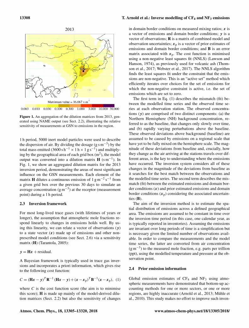
Figure 2. Schematic of the domain borders as applied in the in-version. A total of 11 domain border conditions were estimated asdepicted from 1 to 11 as a multiplying factor to the prior base-line estimated using data from the Mace Head observatory. Be-low 6 km, the domain border was divided eight times: NNE, ENE,ESE, SSE, SSW, WSW, WNW, and NNW; between 6 and 9 km,the domain border was just divided between north and south; andair arriving from above 9 km was considered from one “high” do-main border. Average posterior multiplying factors for CF4 over the8 years were 1.00± 0.01 (NNE), 0.97± 0.06 (ENE), 1.02± 0.05(ESE), 0.99±0.01 (SSE), 1.00±0.01 (SSW), 0.99±0.01 (WSW),1.00± 0.00 (WNW), 1.00± 0.01 (NNW), 1.00± 0.00 (6 to 9 kmnorth), 1.00±0.05 (6 to 9 km south), and 0.97±0.03 (above 9 km).

trace gases, driven mainly by the different emission rates be-tween the two hemispheres and slow interhemispheric mix-ing.

In addition to the time-integrated air concentration pro-duced by NAME (Sect. 2.2), the 3-D coordinate where eachparticle left the computational domain was also recorded.This information was then post-processed to produce the per-centage contributions from 11 different borders of the 3-Ddomain (Fig. 2). From 0 to 6 km in height, eight horizontalboundaries (WSW, WNW, NNW, NNE, ENE, ESE, SSE, andSSW) were considered, and between 6 and 9 km the horizon-tal boundaries were only split between north and south. The11th border was considered when particles left in any direc-tion above 9 km. Thus, the influence of air arriving at GSNfrom outside the domain was simplified as a combination ofair masses arriving from 11 discrete directions.

We use measurements from the Mace Head observatory(from here termed MHD) on the west coast of Ireland(53.33◦ N, 9.90◦W) – a key AGAGE site providing long-term in situ atmospheric measurements – to act as a start-ing point for an estimate of the composition of air from theNH midlatitudes entering the East Asian domain. MHD wasone of the first locations to measure CF4 (starting 2004) andNF3 (starting 2012), and other measurements from the siteare routinely used in atmospheric studies to calculate decadaltrends in the NH atmospheric abundances. In summary, aquadratic fit was made only to MHD observations that wererepresentative of the NH baseline, i.e. when well-mixed airwas arriving predominately from the WNW–NNW (North

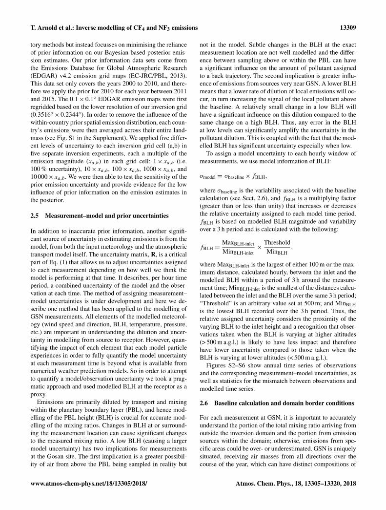
Figure 3. Time series of CF4 measurements during 2013 – an ex-ample year with the most uninterrupted time series. Prior base-line (blue) is adjusted in the inversion using the baseline conditionvariables, producing a posterior baseline (red). During the summermonths, the proportion of air arriving from the south significantlyrises, causing a large shift in the posterior baseline relative to theprior baseline calculated from Mace Head data.

Atlantic) direction as calculated using NAME (details of fil-tering and fitting are given in the Supplement).

The composition of air arriving from any of the 11 direc-tions is calculated using corresponding multiplying factorsapplied to the MHD baseline, which were included as part ofthe state vector (x); i.e. these factors are constant for a giveninversion year. The prior baseline was therefore perturbed aspart of the inversion based on the relative contribution of airarriving from different borders of the 3-D domain and themultiplying factors that are included within the cost function(Eq. 1). Figure 3 shows an annual time series of observationsfor CF4 and the difference between the prior baseline (thequadratic fit from MHD) and the posterior baseline.

2.7 Domains and inversion grids

The domain used in the inversion is smaller than the com-putational NAME transport model domain. The horizon-tal inversion domain covers 88.132 to 145.860◦ E longitude(164 fine grid cells of 0.352◦) and 15.994 to 57.646◦ N lat-itude (178 fine grid cells of 0.234◦). GSN is within a re-gion surrounded by countries with major developed indus-tries, and therefore the site is relatively insensitive to emis-sions from further away that are diluted on the route to thesite. NAME is run on a larger domain to ensure that on theoccasion when air circulates out of the inversion domain andthen back, its full 30-day history in the inversion domain isincluded.

An initial computational inversion grid (from here termedthe “coarse grid”) was created based on (a) aggregated in-formation from the NAME footprints over the period of theinversion (in this case, 1 year), aggregating fewer grid cellsin areas that are “seen” the most by GSN, and (b) the prioremissions flux; i.e. areas known to have low emissions (e.g.ocean) had higher aggregation. Coarse grid cells could notbe aggregated over more than a single country/region and atotal of ≈ 100 coarse grid cells (n) were created. After theinitial inversion, a coarse grid cell was chosen to divide in

Atmos. Chem. Phys., 18, 13305–13320, 2018 www.atmos-chem-phys.net/18/13305/2018/

T. Arnold et al.: Inverse modelling of CF4 and NF3 emissions 13311

two by area. The decision on which single coarse grid cellto split is calculated based on the posterior emission density(g yr−1 m−2) of the coarse grids and the ability of the pos-terior emissions to impact the measurements at GSN (usinginformation from the NAME output). A new inversion wasrun using identical inputs except for the number of grid cells(now n+ 1). This sequence was repeated 50 times, creating≈ 150 coarse grid cells within the inversion domain for thefinal inversion. The results from the inversions with the max-imum disaggregation are presented in this paper.

3 Results and discussion

3.1 Country total emission estimates

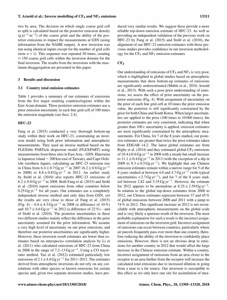
Table 1 provides a summary of our estimates of emissionsfrom the five major emitting countries/regions within theEast Asian domain. These posterior emission estimates use aprior emission uncertainty in each fine grid cell of 100 timesthe emission magnitude (see Sect. 2.4).

HFC-23

Fang et al. (2015) conducted a very thorough bottom-upstudy within their work on HFC-23, constraining an inver-sion model using both prior information and atmosphericmeasurements. They used an inverse method based on theFLEXible PARTicle dispersion model (FLEXPART) usingmeasurements from three sites in East Asia – GSN, Hateruma(a Japanese island∼ 200 km east of Taiwan), and Cape Ochi-ishi (northern Japan), calculating an HFC-23 emission risein China from 6.4± 0.7 Gg yr−1 in 2007 (6.2± 0.6 Gg yr−1

in 2008) to 8.8± 0.8 Gg yr−1 in 2012. An earlier studyby Stohl et al. (2010) also reports HFC-23 emissions of6.2± 0.8 Gg yr−1 in 2008. Both Fang et al. (2015) and Stohlet al. (2010) report emissions from other countries below0.25 Gg yr−1 for all years. Our estimates use a completelyindependent inverse method and only data from GSN, yetthe results are very close to those of Fang et al. (2015)(Fig. 4) – 6.8± 4.3 Gg yr−1 in 2008 (a difference of 10 %)and 10.7± 4.6 Gg yr−1 in 2012 (a difference of 22 %) – andof Stohl et al. (2010). The posterior uncertainties in thesetwo different studies mainly reflect the difference in the prioruncertainty assumed for the prior information. We assumea very high level of uncertainty on our prior emissions, andtherefore our posterior uncertainties are significantly higher.However, these inversion result estimates are lower than es-timates based on interspecies correlation analysis by Li etal. (2011) who calculated emissions of HFC-23 from Chinain 2008 in the range of 7.2–13 Gg yr−1. Using a CO tracer-ratio method, Yao et al. (2012) estimated particularly lowemissions of 2.1±4.6 Gg yr−1 for 2011–2012. The estimatesderived from atmospheric inversions do not rely on any cor-relations with other species or known emissions for certainspecies and, given two separate inversion studies, have pro-

duced very similar results. We suggest these provide a morereliable top-down emission estimate of HFC-23. As well asproviding an independent validation of the previous work onHFC-23 by Fang et al. (2015) and Stohl et al. (2010), thealignment of our HFC-23 emission estimates with those pre-vious studies provides confidence in our inversion methodol-ogy for the CF4 and NF3 emission estimates.

CF4

Our understanding of emissions of CF4 and NF3 is very poor,which is highlighted in global studies based on atmosphericmeasurements that show bottom-up estimates of emissionsare significantly underestimated (Mühle et al., 2010; Arnoldet al., 2013). With such a poor prior understanding of emis-sions, we assess the effect of prior uncertainty on the pos-terior emissions (Fig. 4). With assignment of uncertainty onthe prior of each fine grid cell at 10 times the prior emissionvalue, the posterior is still significantly constrained by theprior for both China and South Korea. When larger uncertain-ties are applied to the prior (100 times to 10 000 times), theposterior estimates are very consistent, indicating that whengreater than 100× uncertainty is applied, emission estimatesare most significantly constrained by the atmospheric mea-surements. For China, for 7 of the 8 years studied, our poste-rior estimates are greater than twice the prior estimates takenfrom EDGAR v4.2. The latest global estimates are fromRigby et al. (2014) and they estimated global CF4 emissionsof 10.4±0.6 Gg yr−1 in 2008 with a steady but small increaseto 11.1± 0.4 Gg yr−1 in 2013 (with the exception of a dip in2009 to 9.3± 0.5 Gg yr−1). We highlight that our Chineseemission estimates remain within a narrow range for 5 of the8 years studied at between 4.0 and 4.7 Gg yr−1 (with typicaluncertainties < 2.7 Gg yr−1), and for 7 of the 8 years stud-ied between 2.82 and 5.35 Gg yr−1. However, the estimatefor 2012 appears to be anomalous at 8.25± 2.59 Gg yr−1.In relation to the global top-down estimates from 2008 to2012, our Chinese estimates represent between 37 and 45 %of global emissions between 2008 and 2011 with a jump to74 % in 2012. This significant increase in 2012 is not recon-cilable with atmospheric measurements on the global scaleand is very likely a spurious result of the inversion. The mostprobable explanation for such a result is the incorrect assign-ment of emissions on the inversion grid. Incorrect assignmentof emissions can occur between countries, particularly whereair parcels frequently pass over more than one country, there-fore reducing the ability of the inversion to confidently placeemissions. However, there is not an obvious drop in emis-sions for another country in 2012 that would offset the largeincrease in the Chinese emission estimate. Within a country,incorrect assignment of emissions from an area closer to thereceptor to an area further from the receptor will increase thecalculated total emissions due to increased dilution in goingfrom a near to a far source. Our inversion is susceptible tothis effect as we only have one site for assimilation of mea-

www.atmos-chem-phys.net/18/13305/2018/ Atmos. Chem. Phys., 18, 13305–13320, 2018

13312 T. Arnold et al.: Inverse modelling of CF4 and NF3 emissions

Table 1. Annual posterior emission estimates for the five main emitting countries surrounding GSN (Gg yr−1). These posterior emissionestimates are from the inversion that uses a prior emission uncertainty on each fine grid cell of 100 times the prior emission rate.

CF4 NF3 HFC-23

China S. Korea N. Korea Japan Taiwan China S. Korea N. Korea Japan Taiwan China S. Korea N. Korea Japan Taiwan

2008 4.66 0.31 0.05 0.57 0.01 6.8 0.09 0.08 0.28 0.11(1.82)∗ (0.05)∗ (0.12)∗ (0.36)∗ (0.07) (4.3) (0.09) (0.28) (0.69) (0.15)

2009 4.01 0.15 0.02 0.23 0.32 5.2 0.04 0.00 0.29 0.00(1.80) (0.05) (0.10) (0.33) (0.17) (5.1) (0.12) (0.29) (0.84) (0.48)

2010 4.42 0.29 0.00 0.10 0.06 9.2 0.04 0.00 0.02 0.00(2.06) (0.05) (0.16) (0.48) (0.13) (6.4) (0.10) (0.39) (1.11) (0.31)

2011 4.12 0.32 0.06 0.18 0.00 8.4 0.09 0.00 0.26 0.00(2.37) (0.05) (0.15) (0.67) (0.26) (5.1) (0.08) (0.27) (0.69) (0.41)

2012 8.25 0.29 0.00 0.16 0.04 10.7 0.10 0.00 0.06 0.24(2.59) (0.05) (0.13) (0.60) (0.40) (4.6) (0.07) (0.23) (0.67) (0.46)

2013 2.82 0.26 0.08 0.11 0.09(2.49) (0.04) (0.13) (0.48) (0.26)

2014 5.35 0.21 0.07 0.21 0.00 1.08 0.40 0.02 0.75 0.03(2.61) (0.05) (0.15) (0.50) (0.30) (1.17) (0.05) (0.12) (0.36) (0.09)

2015 4.33 0.36 0.00 0.36 0.00 0.36 0.60 0.15 0.11 0.00(2.65) (0.11) (0.26) (0.57) (0.44) (1.36) (0.07) (0.16) (0.39) (0.27)

∗ Kim et al. (2010) estimated CF4 emissions from China in the range 1.7–3.1 Gg yr−1 and Li et al. (2011) in the range 1.4–2.9 Gg yr−1. For South and North Korea (combined), Li et al. (2011) estimated emissions of CF4at 0.19–0.26 Gg yr−1 and from Japan at 0.2–0.3 Gg yr−1.

Figure 4. Time series of country emission totals (2008–2015). Annual inversion results are given for each gas for three different levels ofuncertainty applied to the prior emission map: 100, 1000, and 10 000 times the emission magnitude for each grid cell. The aggregated countrytotals from the prior data set are also given. Posterior uncertainties are shown for the 100 times prior uncertainty scenario.

surements; two measurement sites, spaced apart and strad-dling the area of interest, would provide significantly moreinformation to constrain the spatial emission distribution.

Our estimates are significantly higher than emission es-timation methods using interspecies correlation: Kim etal. (2010) estimated CF4 emissions in the range of only 1.7–3.1 Gg yr−1 in 2008 and Li et al. (2011) only 1.4–2.9 Gg yr−1

over the same period. The interspecies correlation approachinherently requires that the sources of the different gasesthat are compared are coincident in time and space. Kim et

al. (2010) and Li et al. (2011) used HCFC-22 as the tracercompound for China with a calculated emission field from aninverse model, and most emissions of this gas originate fromfugitive release from air conditioners and refrigerators. How-ever, CF4 is emitted mostly from point sources in the semi-conductor and aluminium production industries with differ-ent spatial emission distribution within countries, and likelydifferent temporal characteristics compared to HCFC-22.

Emission estimates from South Korea and Japan are 1 or-der of magnitude lower than those from China. For 2008,

Atmos. Chem. Phys., 18, 13305–13320, 2018 www.atmos-chem-phys.net/18/13305/2018/

T. Arnold et al.: Inverse modelling of CF4 and NF3 emissions 13313

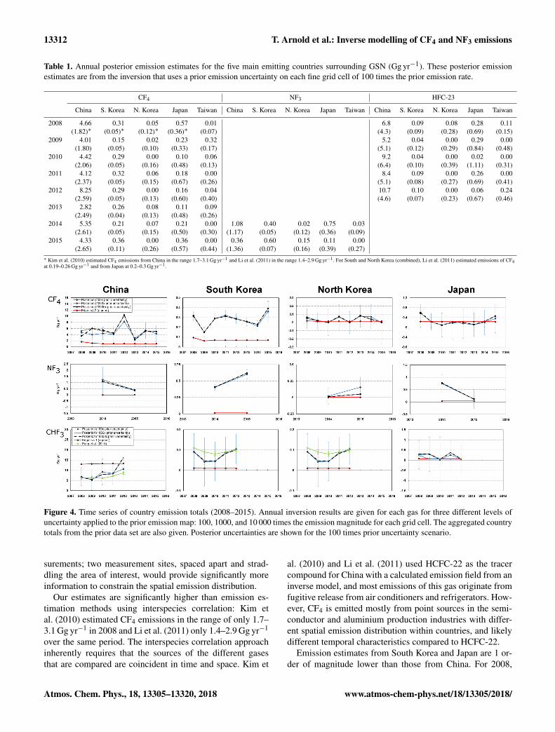
Figure 5. The effect of the regridding routine on posterior emission distributions for CF4. Panels (a), (c), and (e) are posterior emission mapsat the initial inversion resolution, at 0 regridding steps, at 25 regridding steps, and at 50 regridding steps, respectively. Panels (b), (d), and(f) show the emission magnitude minus the uncertainty calculated for each inversion grid box at the same regridding levels (0, 25, and 50),which demonstrates the relative uncertainty of the emission distribution obtained for South Korea. Results are from inversions with initialuncertainty on the prior emission field set to 100 times the emissions at each fine grid square. Units are in g m−2 yr−1.

Li et al. (2011) estimate emissions of CF4 from the combi-nation of South and North Korea of 0.19–0.26 Gg yr−1 andfrom Japan of 0.2–0.3 Gg yr−1, which are on the low endof the uncertainty range of our estimates for that year (Ta-ble 1). As one of the largest, if not the largest, countries forsemiconductor wafer production, Taiwan is also an emitterof CF4. However, measurements at GSN provide only poorsensitivity to detection of emissions from Taiwan, and our re-sults can only suggest that emissions are likely < 0.5 Gg yr−1.North Korean emissions were small and no annual estimatewas above 0.1 Gg yr−1.

NF3

Our understanding of NF3 emissions from inventory and in-dustry data is even poorer than for CF4. On a global scale, theemission estimates from industry are underestimated (Arnoldet al., 2013). This study suggests that at least some emissionsof NF3 stem from China; however, gaining meaningful quan-titative estimates has been difficult due to large uncertainties(Fig. 4). Contrastingly, the posterior estimates of emissionsfrom South Korea have relatively small uncertainties. Emis-sions from China travel a greater distance to the measure-ment site compared to emissions from South Korea. Thus,the magnitudes of NF3 pollution events from China (espe-cially from provinces furthest west), in terms of the mixing

www.atmos-chem-phys.net/18/13305/2018/ Atmos. Chem. Phys., 18, 13305–13320, 2018

13314 T. Arnold et al.: Inverse modelling of CF4 and NF3 emissions

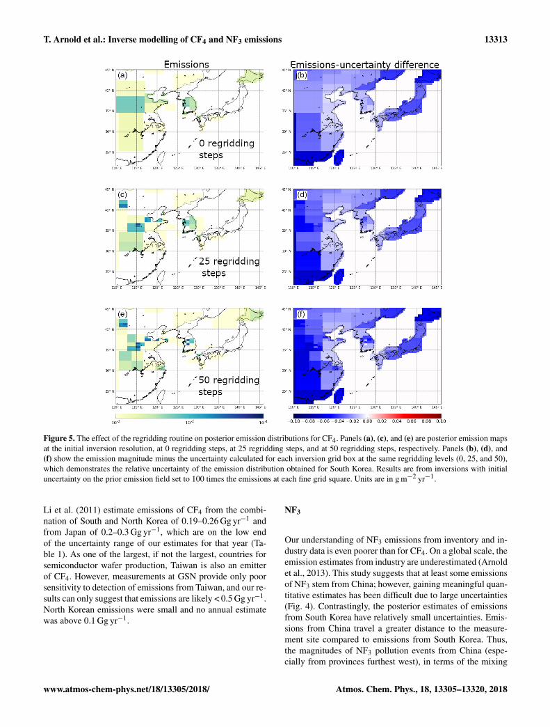
Figure 6. Emission maps for all years of data available for CF4. Results are from inversions with initial uncertainty on the prior emission fieldset to 100 times the emissions at each fine grid square. Units are in g m−2 yr−1; see Fig. S7 for corresponding maps of emission magnitudeminus the uncertainty.

Atmos. Chem. Phys., 18, 13305–13320, 2018 www.atmos-chem-phys.net/18/13305/2018/

T. Arnold et al.: Inverse modelling of CF4 and NF3 emissions 13315

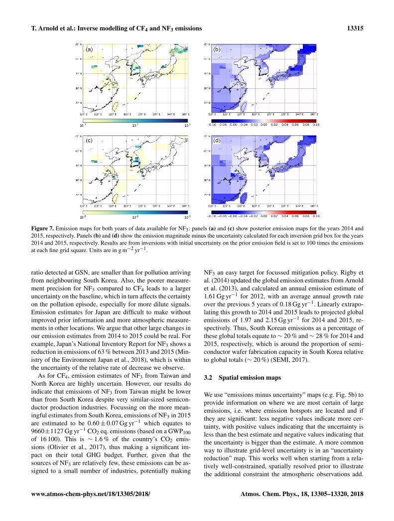
Figure 7. Emission maps for both years of data available for NF3: panels (a) and (c) show posterior emission maps for the years 2014 and2015, respectively. Panels (b) and (d) show the emission magnitude minus the uncertainty calculated for each inversion grid box for the years2014 and 2015, respectively. Results are from inversions with initial uncertainty on the prior emission field is set to 100 times the emissionsat each fine grid square. Units are in g m−2 yr−1.

ratio detected at GSN, are smaller than for pollution arrivingfrom neighbouring South Korea. Also, the poorer measure-ment precision for NF3 compared to CF4 leads to a largeruncertainty on the baseline, which in turn affects the certaintyon the pollution episode, especially for more dilute signals.Emission estimates for Japan are difficult to make withoutimproved prior information and more atmospheric measure-ments in other locations. We argue that other large changes inour emission estimates from 2014 to 2015 could be real. Forexample, Japan’s National Inventory Report for NF3 shows areduction in emissions of 63 % between 2013 and 2015 (Min-istry of the Environment Japan et al., 2018), which is withinthe uncertainty of the relative rate of decrease we observe.

As for CF4, emission estimates of NF3 from Taiwan andNorth Korea are highly uncertain. However, our results doindicate that emissions of NF3 from Taiwan might be lowerthan from South Korea despite very similar-sized semicon-ductor production industries. Focussing on the more mean-ingful estimates from South Korea, emissions of NF3 in 2015are estimated to be 0.60± 0.07 Gg yr−1 which equates to9660±1127 Gg yr−1 CO2 eq. emissions (based on a GWP100of 16 100). This is ∼ 1.6 % of the country’s CO2 emis-sions (Olivier et al., 2017), thus making a significant im-pact on their total GHG budget. Further, given that thesources of NF3 are relatively few, these emissions can be as-signed to a small number of industries, potentially making

NF3 an easy target for focussed mitigation policy. Rigby etal. (2014) updated the global emission estimates from Arnoldet al. (2013), and calculated an annual emission estimate of1.61 Gg yr−1 for 2012, with an average annual growth rateover the previous 5 years of 0.18 Gg yr−1. Linearly extrapo-lating this growth to 2014 and 2015 leads to projected globalemissions of 1.97 and 2.15 Gg yr−1 for 2014 and 2015, re-spectively. Thus, South Korean emissions as a percentage ofthese global totals equate to∼ 20 % and∼ 28 % for 2014 and2015, respectively, which is around the proportion of semi-conductor wafer fabrication capacity in South Korea relativeto global totals (∼ 20 %) (SEMI, 2017).

3.2 Spatial emission maps

We use “emissions minus uncertainty” maps (e.g. Fig. 5b) toprovide information on where we are most certain of largeemissions, i.e. where emission hotspots are located and ifthey are significant: less negative values indicate more cer-tainty, with positive values indicating that the uncertainty isless than the best estimate and negative values indicating thatthe uncertainty is bigger than the estimate. A more commonway to illustrate grid-level uncertainty is in an “uncertaintyreduction” map. This works well when starting from a rela-tively well-constrained, spatially resolved prior to illustratethe additional constraint the atmospheric observations add.

www.atmos-chem-phys.net/18/13305/2018/ Atmos. Chem. Phys., 18, 13305–13320, 2018

13316 T. Arnold et al.: Inverse modelling of CF4 and NF3 emissions

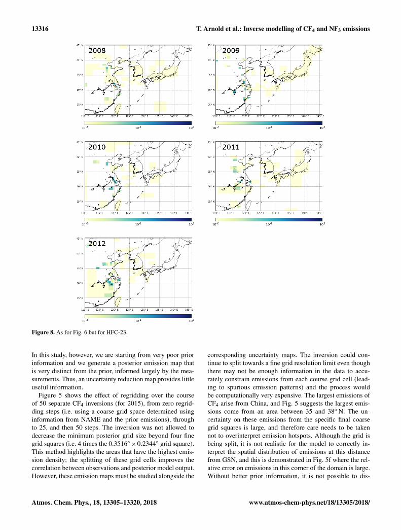
Figure 8. As for Fig. 6 but for HFC-23.

In this study, however, we are starting from very poor priorinformation and we generate a posterior emission map thatis very distinct from the prior, informed largely by the mea-surements. Thus, an uncertainty reduction map provides littleuseful information.

Figure 5 shows the effect of regridding over the courseof 50 separate CF4 inversions (for 2015), from zero regrid-ding steps (i.e. using a coarse grid space determined usinginformation from NAME and the prior emissions), throughto 25, and then 50 steps. The inversion was not allowed todecrease the minimum posterior grid size beyond four finegrid squares (i.e. 4 times the 0.3516◦×0.2344◦ grid square).This method highlights the areas that have the highest emis-sion density; the splitting of these grid cells improves thecorrelation between observations and posterior model output.However, these emission maps must be studied alongside the

corresponding uncertainty maps. The inversion could con-tinue to split towards a fine grid resolution limit even thoughthere may not be enough information in the data to accu-rately constrain emissions from each course grid cell (lead-ing to spurious emission patterns) and the process wouldbe computationally very expensive. The largest emissions ofCF4 arise from China, and Fig. 5 suggests the largest emis-sions come from an area between 35 and 38◦ N. The un-certainty on these emissions from the specific final coarsegrid squares is large, and therefore care needs to be takennot to overinterpret emission hotspots. Although the grid isbeing split, it is not realistic for the model to correctly in-terpret the spatial distribution of emissions at this distancefrom GSN, and this is demonstrated in Fig. 5f where the rel-ative error on emissions in this corner of the domain is large.Without better prior information, it is not possible to dis-

Atmos. Chem. Phys., 18, 13305–13320, 2018 www.atmos-chem-phys.net/18/13305/2018/

T. Arnold et al.: Inverse modelling of CF4 and NF3 emissions 13317

tinguish between real year-to-year emission pattern changesand inaccurate emission patterns (Figs. 6 and S7). Over theperiod of study, emissions of CF4 generally appear to arisefrom north of 30◦ N, and in 2008 and 2013 emissions appeararound 25◦ N. However, GSN does not have good sensitivityto emissions from this area and it is possible that these emis-sions could be incorrectly assigned from Taiwan. Althoughemissions from South Korea are significantly lower than forChina, the proximity to GSN causes the grid cells to be splitand emissions to be assigned at higher spatial resolution andgenerally (except for 2008) in the north-west quadrant of thecountry. Splitting of grid cells in South Korea decreased therelative error on the emissions from particular grid squares,providing confidence that the placement of emissions is accu-rate. Further, for the sequential years 2013, 2014, and 2015,two specific grid cells in that north-west quadrant of SouthKorea are are highlighted with comparatively low uncertain-ties (Fig. S7). How well these consistent year-to-year emis-sion patterns in South Korea correlate with the actual locationof emissions needs to be the subject of further study (e.g. im-proved bottom-up inventory compilation efforts). Emissionsfrom Japan are too uncertain to explore the spatial emissionspattern.

For NF3, emissions from China and Japan are too low anduncertain to interpret at finer spatial resolution. However, aswith CF4, it is interesting to study the relatively more certainspatially disaggregated emissions from South Korea (Fig. 7).In common with CF4, NF3 emissions from the south-westarea are minimal; however, in contrast to CF4, emissions oc-cur on the eastern side of South Korea and on the south-eastcoast. Emissions from the south-east coast coincide with theknown location of a production plant for NF3 located in thearea of Ulsan (Gas World, 2011). If this plant is sufficientlyseparated in space from the end-users of NF3, then this resultwould indicate that production of NF3, not just use, could bea significant source in South Korea.

The study of Fang et al. (2015) highlights three majorhotspots for HFC-23 emissions in China based on HCFC-22 production facility locations. Our posterior maps (Fig. 8)correctly show the bulk of emissions in far eastern China, inline with the results of Fang et al. (2015). However, giventhe inconsistency of emission maps between years, we areunable to provide any more information without a better spa-tially disaggregated prior emission map.

4 Conclusions

We largely remove the influence of bottom-up informationand present the first Bayesian inversion estimates of CF4 andNF3 from the East Asian region using measurements from asingle atmospheric monitoring site, GSN station located onthe island of Jeju (South Korea). The largest CF4 emissionsare from China, estimated at 4–6 Gg yr−1 for 6 out of the8 years studied, which is significantly larger than previous es-

timates. Despite significantly smaller emissions from SouthKorea, the spatial disaggregation of CF4 emissions was con-sistent between independent inversions based on annual mea-surement data sets, indicating the north-west of South Koreais a hotspot for significant CF4 release, presumably from thesemiconductor industry. Emissions of NF3 from South Ko-rea were quantifiable with significant certainty, and representlarge emissions on a CO2 eq. basis (∼ 1.6 % of South Korea’sCO2 emissions in 2015). HFC-23 emissions were also calcu-lated using the same inversion methodology with high uncer-tainty on prior information. We found good agreement withother studies in terms of aggregated country totals and spatialemissions patterns, providing confidence that our methodol-ogy is suitable and our conclusions are justified for estimatesof CF4 and NF3.

Our results highlight an inadequacy in both the bottom-up reported estimates for CF4 and NF3 and the limitationsof the current measurement infrastructure for top-down esti-mates for these specific gases. Adequate bottom-up estimateshave been lacking due to the absence of reporting require-ments for these gases from China and South Korea, and top-down estimates have been hampered by poor measurementcoverage due to the technical complexities required to mea-sure these volatile, low-abundance gases at high precision.Improvements in both bottom-up information and measure-ment coverage, alongside refinements in transport modellingand developments in inversion methodologies, will lead toimproved optimal emission estimates of these gases in futurestudies.

Data availability. Network information and data used in this studyare available from the AGAGE data repository(http://agage.eas.gatech.edu/ or http://cdiac.ess-dive.lbl.gov/ndps/alegage.html, lastaccess: 5 September 2018). See Prinn et al. (2018) for details.

The Supplement related to this article is availableonline at https://doi.org/10.5194/acp-18-13305-2018-supplement.

Author contributions. TA and AJM designed research; TA andAJM performed research; HW and DT contributed towards devel-opment of inversion model; TA, JK, SL, JM, RFW, and SP set upmeasurements; TA, JK, SL, SP, and JM analysed measurement datafrom GSN; and SO analysed measurement data from MHD.

Competing interests. The authors declare that they have no conflictof interest.

www.atmos-chem-phys.net/18/13305/2018/ Atmos. Chem. Phys., 18, 13305–13320, 2018

13318 T. Arnold et al.: Inverse modelling of CF4 and NF3 emissions

Acknowledgements. Observations at GSN were supported by theBasic Science Research Program through the National ResearchFoundation of Korea (NRF) funded by the Ministry of Education(no. NRF-2016R1A2B2010663). The UK’s Department forBusiness, Energy & Industrial Strategy (BEIS) funded the MHDmeasurements and the development of InTEM.

Edited by: Neil HarrisReviewed by: Andreas Stohl and one anonymous referee

References

Arnold, T., Mühle, J., Salameh, P. K., Harth, C. M., Ivy,D. J., and Weiss, R. F.: Automated measurement of nitro-gen trifluoride in ambient air, Anal. Chem., 84, 4798–4804,https://doi.org/10.1021/ac300373e, 2012.

Arnold, T., Harth, C., Mühle, J., Manning, A. J., Salameh, P., Kim,J., Ivy, D. J., Steele, L. P., Petrenko, V. V., Severinghaus, J. P.,Baggenstos, D., and Weiss, R. F.: Nitrogen trifluoride globalemissions estimated from updated atmospheric measurements, P.Natl. Acad. Sci. USA, 110, 2019–2034, 2013.

Bronfin, B. R. and Hazlett, R. N.: Synthesis of nitrogen fluo-rides in a plasma jet, Ind. Eng. Chem. Fund., 5, 472–478,https://doi.org/10.1021/i160020a007, 1966.

Chang, M. B. and Chang, J.-S.: Abatement of PFCs from Semicon-ductor Manufacturing Processes by Nonthermal Plasma Tech-nologies:? A Critical Review, Ind. Eng. Chem. Res., 45, 4101–4109, https://doi.org/10.1021/ie051227b, 2006.

Cullen, M. J. P.: The unified forecast/climate model, Meteorol.Mag., 122, 81–94, 1993.

Deeds, D. A., Vollmer, M. K., Kulongoski, J. T., Miller, B. R.,Muhle, J., Harth, C. M., Izbicki, J. A., Hilton, D. R., and Weiss,R. F.: Evidence for crustal degassing of CF4 and SF6 in MojaveDesert groundwaters, Geochim. Cosmochim. Ac., 72, 999–1013,https://doi.org/10.1016/j.gca.2007.11.027, 2008.

EC-JRC/PBL: Emission Database for Global Atmospheric Re-search (EDGAR), release version 4.2, available at: http://edgar.jrc.ec.europa.eu/ (last access: March 2016), Source: EuropeanCommission, Joint Research Centre (JRC)/Netherlands Environ-mental Assessment Agency (PBL), 2013.

Fang, X., Miller, B. R., Su, S., Wu, J., Zhang, J., and Hu, J.: Histori-cal Emissions of HFC-23 (CHF3) in China and Projections uponPolicy Options by 2050, Environ. Sci. Technol., 48, 4056–4062,https://doi.org/10.1021/es404995f, 2014.

Fang, X., Stohl, A., Yokouchi, Y., Kim, J., Li, S., Saito, T., Park,S., and Hu, J.: Multiannual Top-Down Estimate of HFC-23Emissions in East Asia, Environ. Sci. Technol., 49, 4345–4353,https://doi.org/10.1021/es505669j, 2015.

Gas World: Air Products doubles NF3 facility at Ulsan, Korea, gas-world Publishing LLC, 2011.

Henderson, P. B. and Woytek, A. J.: Nitrogen–nitrogen trifluoride,in: Kirk–Othmer Encyclopedia of Chemical Technology, 4th ed.,edited by: Kroschwitz, J. I. and Howe-Grant, M., John Wiley &Sons, New York, 1994.

Illuzzi, F. and Thewissen, H.: Perfluorocompounds emission reduc-tion by the semiconductor industry, J. Integr. Environ. Sci., 7,201–210, https://doi.org/10.1080/19438151003621417, 2010.

International Aluminium Institute: The International Aluminium In-stitute Report on the Aluminium Industry’s Global Perfluorocar-bon Gas Emissions Reduction Programme – Results of the 2015Anode Effect Survey, International Aluminum Institute, London,1–56, 2016.

International SEMATECH Manufacturing Initiative: Reduction ofPerfluorocompound (PFC) Emissions: 2005 State of the Technol-ogy Report, International SEMATECH Manufacturing Initiative,2005.

Johnson, A. D., Entley, W. R., and Maroulis, P. J.: Reducing PFCgas emissions from CVD chamber cleaning, Solid State Technol.,43, 103–114, 2000.

Jones, A., Thomson, D., Hort, M., and Devenish, B.: The UK MetOffice’s next-generation atmospheric dispersion model, NAMEIII, Air Pollution Modeling and Its Applications Xvii, edited by:Borrego, C. and Norman, A. L., 580–589, 2007.

Keller, C. A., Hill, M., Vollmer, M. K., Henne, S., Brunner, D.,Reimann, S., O’Doherty, S., Arduini, J., Maione, M., Ferenczi,Z., Haszpra, L., Manning, A. J., and Peter, T.: European Emis-sions of Halogenated Greenhouse Gases Inferred from Atmo-spheric Measurements, Environ. Sci. Technol., 46, 217–225,https://doi.org/10.1021/es202453j, 2012.

Kim, J., Li, S., Kim, K. R., Stohl, A., Mühle, J., Kim, S. K.,Park, M. K., Kang, D. J., Lee, G., Harth, C. M., Salameh, P.K., and Weiss, R. F.: Regional atmospheric emissions deter-mined from measurements at Jeju Island, Korea: Halogenatedcompounds from China, Geophys. Res. Lett., 37, L12801,https://doi.org/10.1029/2010gl043263, 2010.

Kim, J., Fraser, P. J., Li, S., Muhle, J., Ganesan, A. L., Krum-mel, P. B., Steele, L. P., Park, S., Kim, S. K., Park, M.K., Arnold, T., Harth, C. M., Salameh, P. K., Prinn, R. G.,Weiss, R. F., and Kim, K. R.: Quantifying aluminum andsemiconductor industry perfluorocarbon emissions from atmo-spheric measurements, Geophys. Res. Lett., 41, 4787–4794,https://doi.org/10.1002/2014gl059783, 2014.

Lawson, C. L. and Hanson, R. J.: Solving Least Squares Problems,Classics in Applied Mathematics, 1974.

Li, S., Kim, J., Kim, K.-R., Muehle, J., Kim, S.-K., Park,M.-K., Stohl, A., Kang, D.-J., Arnold, T., Harth, C. M.,Salameh, P. K., and Weiss, R. F.: Emissions of HalogenatedCompounds in East Asia Determined from Measurements atJeju Island, Korea, Environ. Sci. Technol., 45, 5668–5675,https://doi.org/10.1021/es104124k, 2011.

McCulloch, A. and Lindley, A. A.: Global emissions of HFC-23 estimated to year 2015, Atmos. Environ., 41, 1560–1566,https://doi.org/10.1016/j.atmosenv.2006.02.021, 2007.

Miller, B. R., Weiss, R. F., Salameh, P. K., Tanhua, T., Gre-ally, B. R., Mühle, J., and Simmonds, P. G.: Medusa: Asample preconcentration and GC/MS detector system for insitu measurements of atmospheric trace halocarbons, hydro-carbons, and sulfur compounds, Anal. Chem., 80, 1536–1545,https://doi.org/10.1021/ac702084k, 2008.

Miller, B. R., Rigby, M., Kuijpers, L. J. M., Krummel, P. B.,Steele, L. P., Leist, M., Fraser, P. J., McCulloch, A., Harth, C.,Salameh, P., Mühle, J., Weiss, R. F., Prinn, R. G., Wang, R. H.J., O’Doherty, S., Greally, B. R., and Simmonds, P. G.: HFC-23 (CHF3) emission trend response to HCFC-22 (CHClF2) pro-duction and recent HFC-23 emission abatement measures, At-

Atmos. Chem. Phys., 18, 13305–13320, 2018 www.atmos-chem-phys.net/18/13305/2018/

T. Arnold et al.: Inverse modelling of CF4 and NF3 emissions 13319

mos. Chem. Phys., 10, 7875–7890, https://doi.org/10.5194/acp-10-7875-2010, 2010.

Ministry of the Environment Japan Greenhouse Gas Inventory Of-fice of Japan, Center for Global Environmental Research, andNational Institute for Environmental Studies: National Green-house Gas Inventory Report of JAPAN, 2018.

Montzka, S. A., Kuijpers, L., Battle, M. O., Aydin, M., Verhulst,K. R., Saltzman, E. S., and Fahey, D. W.: Recent increasesin global HFC-23 emissions, Geophys. Res. Lett., 37, L02808,https://doi.org/10.1029/2009gl041195, 2010.

Mühle, J., Ganesan, A. L., Miller, B. R., Salameh, P. K., Harth,C. M., Greally, B. R., Rigby, M., Porter, L. W., Steele, L. P.,Trudinger, C. M., Krummel, P. B., O’Doherty, S., Fraser, P. J.,Simmonds, P. G., Prinn, R. G., and Weiss, R. F.: Perfluorocarbonsin the global atmosphere: tetrafluoromethane, hexafluoroethane,and octafluoropropane, Atmos. Chem. Phys., 10, 5145–5164,https://doi.org/10.5194/acp-10-5145-2010, 2010.

Myhre, G., Shindell, D., Bréon, F.-M., Collins, W., Fuglestvedt,J., Huang, J., Koch, D., Lamarque, J.-F., Lee, D., Mendoza,B., Nakajima, T., Robock, A., Stephens, G., Takemura, T., andZhang, H.: Anthropogenic and Natural Radiative Forcing, in:Climate Change 2013: The Physical Science Basis, Contributionof Working Group I to the Fifth Assessment Report of the Inter-governmental Panel on Climate Change, edited by: Stocker, T.F., Qin, D., Plattner, G.-K., Tignor, M., Allen, S. K., Boschung,J., Nauels, A., Xia, Y., Bex, V., and Midgley, P. M., CambridgeUniversity Press, Cambridge, United Kingdom and New York,NY, USA, 659–740, 2013.

Olivier, J. G. J., Schure, K. M., and Peters, J. A. H. W.: Trends inglobal CO2 emissions; 2017 Report, PBL Netherlands Environ-mental Assessment Agency, The Hague/Bilthoven500114022,2017.

Prinn, R. G., Weiss, R. F., Arduini, J., Arnold, T., DeWitt, H. L.,Fraser, P. J., Ganesan, A. L., Gasore, J., Harth, C. M., Her-mansen, O., Kim, J., Krummel, P. B., Li, S., Loh, Z. M., Lun-der, C. R., Maione, M., Manning, A. J., Miller, B. R., Mitrevski,B., Mühle, J., O’Doherty, S., Park, S., Reimann, S., Rigby, M.,Saito, T., Salameh, P. K., Schmidt, R., Simmonds, P. G., Steele,L. P., Vollmer, M. K., Wang, R. H., Yao, B., Yokouchi, Y., Young,D., and Zhou, L.: History of chemically and radiatively impor-tant atmospheric gases from the Advanced Global AtmosphericGases Experiment (AGAGE), Earth Syst. Sci. Data, 10, 985–1018, https://doi.org/10.5194/essd-10-985-2018, 2018.

Purohit, P. and Höglund-Isaksson, L.: Global emissions of flu-orinated greenhouse gases 2005–2050 with abatement po-tentials and costs, Atmos. Chem. Phys., 17, 2795–2816,https://doi.org/10.5194/acp-17-2795-2017, 2017.

Raoux, S.: Implementing technologies for reducing PFC emissions,Solid State Technol., 50, 49–52, 2007.

Rigby, M., Prinn, R. G., O’Doherty, S., Miller, B. R., Ivy, D.,Muhle, J., Harth, C. M., Salameh, P. K., Arnold, T., Weiss, R.F., Krummel, P. B., Steele, L. P., Fraser, P. J., Young, D., andSimmonds, P. G.: Recent and future trends in synthetic green-house gas radiative forcing, Geophys. Res. Lett., 41, 2623–2630,https://doi.org/10.1002/2013gl059099, 2014.

Ryall, D. B. and Maryon, R. H.: Validation of the UK Met. Of-fice’s name model against the ETEX dataset, Atmos. Environ.,32, 4265–4276, https://doi.org/10.1016/s1352-2310(98)00177-0, 1998.

SEMI: SEMI® World Fab Forecast, edited by: SEMI, available at:http://www.semi.org/en/Store/MarketInformation/fabdatabase/ctr_027238 (last access: January 2018), 2017.

Simmonds, P. G., Rigby, M., McCulloch, A., Vollmer, M. K.,Henne, S., Mühle, J., O’Doherty, S., Manning, A. J., Krum-mel, P. B., Fraser, P. J., Young, D., Weiss, R. F., Salameh, P.K., Harth, C. M., Reimann, S., Trudinger, C. M., Steele, L.P., Wang, R. H. J., Ivy, D. J., Prinn, R. G., Mitrevski, B., andEtheridge, D. M.: Recent increases in the atmospheric growthrate and emissions of HFC-23 (CHF3) and the link to HCFC-22 (CHClF2) production, Atmos. Chem. Phys., 18, 4153–4169,https://doi.org/10.5194/acp-18-4153-2018, 2018.

Stohl, A., Kim, J., Li, S., O’Doherty, S., Mühle, J., Salameh,P. K., Saito, T., Vollmer, M. K., Wan, D., Weiss, R. F.,Yao, B., Yokouchi, Y., and Zhou, L. X.: Hydrochlorofluoro-carbon and hydrofluorocarbon emissions in East Asia deter-mined by inverse modeling, Atmos. Chem. Phys., 10, 3545–3560, https://doi.org/10.5194/acp-10-3545-2010, 2010.

Thomson, D. J., Webster, H. N., and Cooke, M. C.: Developmentsin the Met Office InTEM volcanic ash source estimation system,Part 1: Concepts Met Office, 2017.

Totterdill, A., Kovács, T., Feng, W., Dhomse, S., Smith, C. J.,Gómez-Martín, J. C., Chipperfield, M. P., Forster, P. M., andPlane, J. M. C.: Atmospheric lifetimes, infrared absorption spec-tra, radiative forcings and global warming potentials of NF3 andCF3CF2Cl (CFC-115), Atmos. Chem. Phys., 16, 11451–11463,https://doi.org/10.5194/acp-16-11451-2016, 2016.

Vogel, H., Flerus, B., Stoffner, F., and Friedrich, B.: Re-ducing Greenhouse Gas Emission from the NeodymiumOxide Electrolysis. Part I: Analysis of the Anodic GasFormation, Journal of Sustainable Metallurgy, 3, 99–107,https://doi.org/10.1007/s40831-016-0086-0, 2017.

Wangxing, L., Xiping, C., Shilin, Q., Baowei, Z., and Bayliss, C.:Reduction Strategies for PFC Emissions from Chinese Smelters,in: Light Metals 2013, edited by: Sadler, B. A., Springer Interna-tional Publishing, Cham, 893–898, 2016.

Webster, H. N., Thomson, D. J., and Cooke, M. C.: Developmentsin the Met Office InTEMvolcanic ash source estimation system,Part 2: Results, Met Office, 2017.

World Semiconductor Council: Joint Statement of the 21st Meet-ing of the World Semiconductor Council (WSC), Kyoto, Japan,2017.

Worton, D. R., Sturges, W. T., Gohar, L. K., Shine, K. P., Mar-tinerie, P., Oram, D. E., Humphrey, S. P., Begley, P., Gunn,L., Barnola, J.-M., Schwander, J., and Mulvaney, R.: Atmo-spheric Trends and Radiative Forcings of CF4 and C2F6 In-ferred from Firn Air, Environ. Sci. Technol., 41, 2184–2189,https://doi.org/10.1021/es061710t, 2007.

Yang, C.-F. O., Kam, S.-H., Liu, C.-H., Tzou, J., andWang, J.-L.: Assessment of removal efficiency of per-fluorocompounds (PFCs) in a semiconductor fabricationplant by gas chromatography, Chemosphere, 76, 1273–1277,https://doi.org/10.1016/j.chemosphere.2009.06.039, 2009.

Yao, B., Vollmer, M. K., Zhou, L. X., Henne, S., Reimann, S., Li,P. C., Wenger, A., and Hill, M.: In-situ measurements of atmo-spheric hydrofluorocarbons (HFCs) and perfluorocarbons (PFCs)at the Shangdianzi regional background station, China, Atmos.Chem. Phys., 12, 10181–10193, https://doi.org/10.5194/acp-12-10181-2012, 2012.

www.atmos-chem-phys.net/18/13305/2018/ Atmos. Chem. Phys., 18, 13305–13320, 2018

13320 T. Arnold et al.: Inverse modelling of CF4 and NF3 emissions

Yokouchi, Y., Taguchi, S., Saito, T., Tohjima, Y., Tani-moto, H., and Mukai, H.: High frequency measurements ofHFCs at a remote site in east Asia and their implicationsfor Chinese emissions, Geophys. Res. Lett., 33, L21814,https://doi.org/10.1029/2006GL026403, 2006.

Zhang, L., Wang, X., and Gong, B.: Perfluorocarbon emis-sions from electrolytic reduction of rare earth metalsin fluoride/oxide system, Atmos. Pollut. Res., 61–65,https://doi.org/10.1016/j.apr.2017.06.006, 2017.

Atmos. Chem. Phys., 18, 13305–13320, 2018 www.atmos-chem-phys.net/18/13305/2018/