Embed Size (px)
Citation preview
SANDIA REPORTSAND2007-2734Unlimited ReleasePrinted April 24, 2007
Aria 1.5: User Manual
Patrick K. Notz, Samuel R. Subia, Matthew M. Hopkins, Harry K. Moffat, David R.Noble
Prepared bySandia National LaboratoriesAlbuquerque, New Mexico 87185 and Livermore, California 94550
Sandia is a multiprogram laboratory operated by Sandia Corporation,a Lockheed Martin Company, for the United States Department of Energy’sNational Nuclear Security Administration under Contract DE-AC04-94-AL85000.
Approved for public release; further dissemination unlimited.
Issued by Sandia National Laboratories, operated for the United States Department of Energy by SandiaCorporation.
NOTICE: This report was prepared as an account of work sponsored by an agency of the United StatesGovernment. Neither the United States Government, nor any agency thereof, nor any of their employees,nor any of their contractors, subcontractors, or their employees, make any warranty, express or implied,or assume any legal liability or responsibility for the accuracy, completeness, or usefulness of any infor-mation, apparatus, product, or process disclosed, or represent that its use would not infringe privatelyowned rights. Reference herein to any specific commercial product, process, or service by trade name,trademark, manufacturer, or otherwise, does not necessarily constitute or imply its endorsement, recom-mendation, or favoring by the United States Government, any agency thereof, or any of their contractorsor subcontractors. The views and opinions expressed herein do not necessarily state or reflect those ofthe United States Government, any agency thereof, or any of their contractors.
Printed in the United States of America. This report has been reproduced directly from the best availablecopy.
Available to DOE and DOE contractors fromU.S. Department of EnergyOffice of Scientific and Technical InformationP.O. Box 62Oak Ridge, TN 37831
Telephone: (865) 576-8401Facsimile: (865) 576-5728E-Mail: [email protected] ordering: http://www.osti.gov/bridge
Available to the public fromU.S. Department of CommerceNational Technical Information Service5285 Port Royal RdSpringfield, VA 22161
Telephone: (800) 553-6847Facsimile: (703) 605-6900E-Mail: [email protected] ordering: http://www.ntis.gov/help/ordermethods.asp?loc=7-4-0#online
DE
PA
RT
MENT OF EN
ER
GY
• • UN
IT
ED
STATES OFA
M
ER
IC
A
2
SAND2007-2734Unlimited Release
Printed April 24, 2007
Aria 1.5: User Manual
Patrick K. Notz, Samuel R. Subia, Matthew M. Hopkins, Harry K. Moffat, David R. NobleSandia National Laboratories
P.O. Box 5800Albuquerque, NM 87185
Abstract
Aria is a Galerkin finite element based program for solving coupled-physics problems described bysystems of PDEs and is capable of solving nonlinear, implicit, transient and direct-to-steady stateproblems in two and three dimensions on parallel architectures. The suite of physics currentlysupported by Aria includes the incompressible Navier-Stokes equations, energy transport equation,species transport equations, nonlinear elastic solid mechanics, and electrostatics as well as general-ized scalar, vector and tensor transport equations. Additionally, Aria includes support for arbitraryLagrangian-Eulerian (ALE) and level set based free and moving boundary tracking. Coupled physicsproblems are solved in several ways including fully-coupled Newton’s method with analytic or nu-merical sensitivities, fully-coupled Newton-Krylov methods, fully-coupled Picard’s method, and aloosely-coupled nonlinear iteration about subsets of the system that are solved using combinationsof the aforementioned methods. Error estimation, uniform and dynamic h-adaptivity and dynamicload balancing are some of Aria’s more advanced capabilities. Aria is based on the Sierra Framework.
3
Contents
Contents 4
List of Figures 13
List of Tables 14
1 Introduction 15
1.1 Aria Overview . . . . . . . . . . . . . . . . . . . . . . . . . . . . . . . . . . . . . . . . . . . . . . . . . . . . . . . . . 15
1.2 Nonlinear Coupling Strategies in Aria . . . . . . . . . . . . . . . . . . . . . . . . . . . . . . . . . . . . . . 15
1.3 Constraints Equations within Aria . . . . . . . . . . . . . . . . . . . . . . . . . . . . . . . . . . . . . . . . 16
1.4 Level Set Algorithm . . . . . . . . . . . . . . . . . . . . . . . . . . . . . . . . . . . . . . . . . . . . . . . . . . . . 16
1.5 Outline of the Manual . . . . . . . . . . . . . . . . . . . . . . . . . . . . . . . . . . . . . . . . . . . . . . . . . . . 17
2 Getting Started 19
2.1 Setting Up Your Environment . . . . . . . . . . . . . . . . . . . . . . . . . . . . . . . . . . . . . . . . . . . . 19
2.2 Running Aria . . . . . . . . . . . . . . . . . . . . . . . . . . . . . . . . . . . . . . . . . . . . . . . . . . . . . . . . . . 19
2.3 Aria Environment Overview . . . . . . . . . . . . . . . . . . . . . . . . . . . . . . . . . . . . . . . . . . . . . . 20
2.4 Parallel Processing Runtime Environment . . . . . . . . . . . . . . . . . . . . . . . . . . . . . . . . . . 21
2.5 Overview of the Input File Structure . . . . . . . . . . . . . . . . . . . . . . . . . . . . . . . . . . . . . . . 21
2.6 Fields . . . . . . . . . . . . . . . . . . . . . . . . . . . . . . . . . . . . . . . . . . . . . . . . . . . . . . . . . . . . . . . . 26
2.7 Equations . . . . . . . . . . . . . . . . . . . . . . . . . . . . . . . . . . . . . . . . . . . . . . . . . . . . . . . . . . . . . 26
2.8 Equation String-Naming Convention . . . . . . . . . . . . . . . . . . . . . . . . . . . . . . . . . . . . . . . 26
2.9 Example Program Directory . . . . . . . . . . . . . . . . . . . . . . . . . . . . . . . . . . . . . . . . . . . . . . 28
2.10 Aprepro Interface . . . . . . . . . . . . . . . . . . . . . . . . . . . . . . . . . . . . . . . . . . . . . . . . . . . . . . 28
3 Equations Aria Solves 29
3.1 Generalized Conservation Equation . . . . . . . . . . . . . . . . . . . . . . . . . . . . . . . . . . . . . . . . 29
3.2 Conservation of Mass . . . . . . . . . . . . . . . . . . . . . . . . . . . . . . . . . . . . . . . . . . . . . . . . . . . 29
3.3 Conservation of Energy . . . . . . . . . . . . . . . . . . . . . . . . . . . . . . . . . . . . . . . . . . . . . . . . . . 30
4
3.4 Conservation of Chemical Species . . . . . . . . . . . . . . . . . . . . . . . . . . . . . . . . . . . . . . . . . 31
3.5 Conservation of Fluid Momentum . . . . . . . . . . . . . . . . . . . . . . . . . . . . . . . . . . . . . . . . . 32
3.6 Conservation of Solid Momentum . . . . . . . . . . . . . . . . . . . . . . . . . . . . . . . . . . . . . . . . . 33
3.7 Voltage Equation . . . . . . . . . . . . . . . . . . . . . . . . . . . . . . . . . . . . . . . . . . . . . . . . . . . . . . . 33
3.8 Current Equation . . . . . . . . . . . . . . . . . . . . . . . . . . . . . . . . . . . . . . . . . . . . . . . . . . . . . . 34
3.9 Suspension Equation . . . . . . . . . . . . . . . . . . . . . . . . . . . . . . . . . . . . . . . . . . . . . . . . . . . . 34
3.10 Stress Tensor Projection Equation . . . . . . . . . . . . . . . . . . . . . . . . . . . . . . . . . . . . . . . . . 35
3.11 Notes on Solid Mechanics . . . . . . . . . . . . . . . . . . . . . . . . . . . . . . . . . . . . . . . . . . . . . . . . 36
3.12 Units and Unit Conversions . . . . . . . . . . . . . . . . . . . . . . . . . . . . . . . . . . . . . . . . . . . . . . 38
4 Equation Specification 43
4.1 EQ CONTINUITY . . . . . . . . . . . . . . . . . . . . . . . . . . . . . . . . . . . . . . . . . . . . . . . . . . . . . 43
4.2 EQ CURRENT . . . . . . . . . . . . . . . . . . . . . . . . . . . . . . . . . . . . . . . . . . . . . . . . . . . . . . . . 44
4.3 EQ ENERGY . . . . . . . . . . . . . . . . . . . . . . . . . . . . . . . . . . . . . . . . . . . . . . . . . . . . . . . . . 44
4.4 EQ LEVEL SET . . . . . . . . . . . . . . . . . . . . . . . . . . . . . . . . . . . . . . . . . . . . . . . . . . . . . . . 45
4.5 EQ MESH . . . . . . . . . . . . . . . . . . . . . . . . . . . . . . . . . . . . . . . . . . . . . . . . . . . . . . . . . . . . 45
4.6 EQ MOMENTUM . . . . . . . . . . . . . . . . . . . . . . . . . . . . . . . . . . . . . . . . . . . . . . . . . . . . . 46
4.7 EQ SHEAR . . . . . . . . . . . . . . . . . . . . . . . . . . . . . . . . . . . . . . . . . . . . . . . . . . . . . . . . . . . 46
4.8 EQ SOLID . . . . . . . . . . . . . . . . . . . . . . . . . . . . . . . . . . . . . . . . . . . . . . . . . . . . . . . . . . . . 47
4.9 EQ SPECIES . . . . . . . . . . . . . . . . . . . . . . . . . . . . . . . . . . . . . . . . . . . . . . . . . . . . . . . . . . 47
4.10 EQ SUSPENSON . . . . . . . . . . . . . . . . . . . . . . . . . . . . . . . . . . . . . . . . . . . . . . . . . . . . . . 48
4.11 EQ VOLTAGE . . . . . . . . . . . . . . . . . . . . . . . . . . . . . . . . . . . . . . . . . . . . . . . . . . . . . . . . 48
4.12 EQ Stress Tensor Projection . . . . . . . . . . . . . . . . . . . . . . . . . . . . . . . . . . . . . . . . . . . . . 49
4.13 ELASTICITY FORMULATION . . . . . . . . . . . . . . . . . . . . . . . . . . . . . . . . . . . . . . . . . . 49
4.14 PRESSURE STABILIZATION . . . . . . . . . . . . . . . . . . . . . . . . . . . . . . . . . . . . . . . . . . . 50
4.15 MESH MOTION . . . . . . . . . . . . . . . . . . . . . . . . . . . . . . . . . . . . . . . . . . . . . . . . . . . . . . . 50
4.16 SAVE RESIDUALS . . . . . . . . . . . . . . . . . . . . . . . . . . . . . . . . . . . . . . . . . . . . . . . . . . . . . 51
4.17 INTEGRATION RULE . . . . . . . . . . . . . . . . . . . . . . . . . . . . . . . . . . . . . . . . . . . . . . . . . 51
5 Initial Conditions 53
5.1 IC CIRC X . . . . . . . . . . . . . . . . . . . . . . . . . . . . . . . . . . . . . . . . . . . . . . . . . . . . . . . . . . . 53
5.2 IC CIRC Y . . . . . . . . . . . . . . . . . . . . . . . . . . . . . . . . . . . . . . . . . . . . . . . . . . . . . . . . . . . 53
5.3 IC CONSTANT . . . . . . . . . . . . . . . . . . . . . . . . . . . . . . . . . . . . . . . . . . . . . . . . . . . . . . . . 54
5
5.4 IC COUETTE X . . . . . . . . . . . . . . . . . . . . . . . . . . . . . . . . . . . . . . . . . . . . . . . . . . . . . . . 54
5.5 IC COUETTE Y . . . . . . . . . . . . . . . . . . . . . . . . . . . . . . . . . . . . . . . . . . . . . . . . . . . . . . . 54
5.6 IC COUETTE SH . . . . . . . . . . . . . . . . . . . . . . . . . . . . . . . . . . . . . . . . . . . . . . . . . . . . . . 55
5.7 IC READ FILE . . . . . . . . . . . . . . . . . . . . . . . . . . . . . . . . . . . . . . . . . . . . . . . . . . . . . . . . 55
5.8 IC LINEAR . . . . . . . . . . . . . . . . . . . . . . . . . . . . . . . . . . . . . . . . . . . . . . . . . . . . . . . . . . . 55
5.9 IC PARAB . . . . . . . . . . . . . . . . . . . . . . . . . . . . . . . . . . . . . . . . . . . . . . . . . . . . . . . . . . . . 56
6 Boundary Conditions 57
6.1 BC CIRC X . . . . . . . . . . . . . . . . . . . . . . . . . . . . . . . . . . . . . . . . . . . . . . . . . . . . . . . . . . . 57
6.2 BC CIRC Y . . . . . . . . . . . . . . . . . . . . . . . . . . . . . . . . . . . . . . . . . . . . . . . . . . . . . . . . . . . 57
6.3 BC CONST . . . . . . . . . . . . . . . . . . . . . . . . . . . . . . . . . . . . . . . . . . . . . . . . . . . . . . . . . . . 58
6.4 BC LINEAR . . . . . . . . . . . . . . . . . . . . . . . . . . . . . . . . . . . . . . . . . . . . . . . . . . . . . . . . . . 58
6.5 BC LINEAR IN TIME . . . . . . . . . . . . . . . . . . . . . . . . . . . . . . . . . . . . . . . . . . . . . . . . . . 58
6.6 BC PARAB . . . . . . . . . . . . . . . . . . . . . . . . . . . . . . . . . . . . . . . . . . . . . . . . . . . . . . . . . . . 59
6.7 BC PERIODIC LINEAR IN TIME. . . . . . . . . . . . . . . . . . . . . . . . . . . . . . . . . . . . . . . . 59
6.8 BC PERIODIC STEP IN TIME . . . . . . . . . . . . . . . . . . . . . . . . . . . . . . . . . . . . . . . . . . 60
6.9 BC ROTATING X . . . . . . . . . . . . . . . . . . . . . . . . . . . . . . . . . . . . . . . . . . . . . . . . . . . . . 60
6.10 BC ROTATING Y . . . . . . . . . . . . . . . . . . . . . . . . . . . . . . . . . . . . . . . . . . . . . . . . . . . . . 61
6.11 BC TRANSLATE . . . . . . . . . . . . . . . . . . . . . . . . . . . . . . . . . . . . . . . . . . . . . . . . . . . . . . 61
6.12 BC UNIDIRECTIONAL FLOW X . . . . . . . . . . . . . . . . . . . . . . . . . . . . . . . . . . . . . . . . 61
6.13 BC UNIDIRECTIONAL FLOW Y . . . . . . . . . . . . . . . . . . . . . . . . . . . . . . . . . . . . . . . . 62
6.14 BC FLUX . . . . . . . . . . . . . . . . . . . . . . . . . . . . . . . . . . . . . . . . . . . . . . . . . . . . . . . . . . . . 63
7 Distinguishing Conditions 73
7.1 An Introduction to Distinguishing Conditions . . . . . . . . . . . . . . . . . . . . . . . . . . . . . . . 73
7.2 BC DISTING . . . . . . . . . . . . . . . . . . . . . . . . . . . . . . . . . . . . . . . . . . . . . . . . . . . . . . . . . . 73
8 Source Terms 77
8.1 POINT SOURCE FOR . . . . . . . . . . . . . . . . . . . . . . . . . . . . . . . . . . . . . . . . . . . . . . . . . 77
8.2 SOURCE FOR ENERGY . . . . . . . . . . . . . . . . . . . . . . . . . . . . . . . . . . . . . . . . . . . . . . . . 77
8.3 SOURCE FOR MOMENTUM . . . . . . . . . . . . . . . . . . . . . . . . . . . . . . . . . . . . . . . . . . . . 81
8.4 SOURCE FOR CURRENT . . . . . . . . . . . . . . . . . . . . . . . . . . . . . . . . . . . . . . . . . . . . . . 83
8.5 SOURCE FOR SPECIES . . . . . . . . . . . . . . . . . . . . . . . . . . . . . . . . . . . . . . . . . . . . . . . . 84
6
8.6 SOURCE FOR VOLTAGE . . . . . . . . . . . . . . . . . . . . . . . . . . . . . . . . . . . . . . . . . . . . . . . 86
9 Constraint Conditions 87
9.1 CONSTRAIN . . . . . . . . . . . . . . . . . . . . . . . . . . . . . . . . . . . . . . . . . . . . . . . . . . . . . . . . . 87
10 Material Properties 89
10.1 BETA . . . . . . . . . . . . . . . . . . . . . . . . . . . . . . . . . . . . . . . . . . . . . . . . . . . . . . . . . . . . . . . . 89
10.2 BULK VISCOSITY . . . . . . . . . . . . . . . . . . . . . . . . . . . . . . . . . . . . . . . . . . . . . . . . . . . . 90
10.3 CTE . . . . . . . . . . . . . . . . . . . . . . . . . . . . . . . . . . . . . . . . . . . . . . . . . . . . . . . . . . . . . . . . . 91
10.4 CURRENT DENSITY . . . . . . . . . . . . . . . . . . . . . . . . . . . . . . . . . . . . . . . . . . . . . . . . . . 92
10.5 DENSITY . . . . . . . . . . . . . . . . . . . . . . . . . . . . . . . . . . . . . . . . . . . . . . . . . . . . . . . . . . . . 93
10.6 ELECTRICAL CONDUCTIVITY . . . . . . . . . . . . . . . . . . . . . . . . . . . . . . . . . . . . . . . . 97
10.7 ELECTRIC DISPLACEMENT . . . . . . . . . . . . . . . . . . . . . . . . . . . . . . . . . . . . . . . . . . . 99
10.8 ELECTRICAL PERMITTIVITY . . . . . . . . . . . . . . . . . . . . . . . . . . . . . . . . . . . . . . . . . 100
10.9 ELECTRICAL RESISTANCE . . . . . . . . . . . . . . . . . . . . . . . . . . . . . . . . . . . . . . . . . . . . 101
10.10 EMISSIVITY . . . . . . . . . . . . . . . . . . . . . . . . . . . . . . . . . . . . . . . . . . . . . . . . . . . . . . . . . . 103
10.11 ENTHALPHY . . . . . . . . . . . . . . . . . . . . . . . . . . . . . . . . . . . . . . . . . . . . . . . . . . . . . . . . . 104
10.12 EQUATION OF STATE . . . . . . . . . . . . . . . . . . . . . . . . . . . . . . . . . . . . . . . . . . . . . . . . . 104
10.13 HEAT CONDUCTION . . . . . . . . . . . . . . . . . . . . . . . . . . . . . . . . . . . . . . . . . . . . . . . . . . 105
10.14 HEAT OF VAPORIZATION . . . . . . . . . . . . . . . . . . . . . . . . . . . . . . . . . . . . . . . . . . . . . 106
10.15 INTRINSIC PERMEABILITY . . . . . . . . . . . . . . . . . . . . . . . . . . . . . . . . . . . . . . . . . . . 106
10.16 INTERNAL ENERGY . . . . . . . . . . . . . . . . . . . . . . . . . . . . . . . . . . . . . . . . . . . . . . . . . . 107
10.17 LAMBDA. . . . . . . . . . . . . . . . . . . . . . . . . . . . . . . . . . . . . . . . . . . . . . . . . . . . . . . . . . . . . 108
10.18 LEVEL SET HEAVISIDE . . . . . . . . . . . . . . . . . . . . . . . . . . . . . . . . . . . . . . . . . . . . . . . 109
10.19 LEVEL SET WIDTH . . . . . . . . . . . . . . . . . . . . . . . . . . . . . . . . . . . . . . . . . . . . . . . . . . . 109
10.20 MASS FLUX . . . . . . . . . . . . . . . . . . . . . . . . . . . . . . . . . . . . . . . . . . . . . . . . . . . . . . . . . . 110
10.21 MESH STRESS . . . . . . . . . . . . . . . . . . . . . . . . . . . . . . . . . . . . . . . . . . . . . . . . . . . . . . . . 110
10.22 MOLECULAR WEIGHT . . . . . . . . . . . . . . . . . . . . . . . . . . . . . . . . . . . . . . . . . . . . . . . . 113
10.23 MOMENTUM STRESS . . . . . . . . . . . . . . . . . . . . . . . . . . . . . . . . . . . . . . . . . . . . . . . . . 114
10.24 POISSONS RATIO . . . . . . . . . . . . . . . . . . . . . . . . . . . . . . . . . . . . . . . . . . . . . . . . . . . . . 116
10.25 POROSITY . . . . . . . . . . . . . . . . . . . . . . . . . . . . . . . . . . . . . . . . . . . . . . . . . . . . . . . . . . . 117
10.26 RELATIVE PERMEABILITY . . . . . . . . . . . . . . . . . . . . . . . . . . . . . . . . . . . . . . . . . . . 118
10.27 SKELETON DENSITY . . . . . . . . . . . . . . . . . . . . . . . . . . . . . . . . . . . . . . . . . . . . . . . . . 119
7
10.28 SKELETON INTERNAL ENERGY . . . . . . . . . . . . . . . . . . . . . . . . . . . . . . . . . . . . . . . 120
10.29 SOLID STRESS . . . . . . . . . . . . . . . . . . . . . . . . . . . . . . . . . . . . . . . . . . . . . . . . . . . . . . . 121
10.30 SPECIES DIFFUSION . . . . . . . . . . . . . . . . . . . . . . . . . . . . . . . . . . . . . . . . . . . . . . . . . . 123
10.31 SPECIES DIFFUSIVITY . . . . . . . . . . . . . . . . . . . . . . . . . . . . . . . . . . . . . . . . . . . . . . . . 124
10.32 SPECIFIC HEAT . . . . . . . . . . . . . . . . . . . . . . . . . . . . . . . . . . . . . . . . . . . . . . . . . . . . . . 125
10.33 SURFACE TENSION . . . . . . . . . . . . . . . . . . . . . . . . . . . . . . . . . . . . . . . . . . . . . . . . . . . 128
10.34 SUSPENSION FLUX . . . . . . . . . . . . . . . . . . . . . . . . . . . . . . . . . . . . . . . . . . . . . . . . . . . 128
10.35 THERMAL CONDUCTIVITY . . . . . . . . . . . . . . . . . . . . . . . . . . . . . . . . . . . . . . . . . . . 129
10.36 THERMAL DIFFUSIVITY . . . . . . . . . . . . . . . . . . . . . . . . . . . . . . . . . . . . . . . . . . . . . . 132
10.37 TOTAL INTERNAL ENERGY . . . . . . . . . . . . . . . . . . . . . . . . . . . . . . . . . . . . . . . . . . . 132
10.38 TWO MU. . . . . . . . . . . . . . . . . . . . . . . . . . . . . . . . . . . . . . . . . . . . . . . . . . . . . . . . . . . . . 133
10.39 VALENCE . . . . . . . . . . . . . . . . . . . . . . . . . . . . . . . . . . . . . . . . . . . . . . . . . . . . . . . . . . . . 134
10.40 VISCOSITY. . . . . . . . . . . . . . . . . . . . . . . . . . . . . . . . . . . . . . . . . . . . . . . . . . . . . . . . . . . 134
10.41 YOUNGS MODULUS . . . . . . . . . . . . . . . . . . . . . . . . . . . . . . . . . . . . . . . . . . . . . . . . . . 141
11 Solution Control Reference 143
11.1 TRANSFER . . . . . . . . . . . . . . . . . . . . . . . . . . . . . . . . . . . . . . . . . . . . . . . . . . . . . . . . . . 143
11.2 SOLUTION CONTROL DESCRIPTION . . . . . . . . . . . . . . . . . . . . . . . . . . . . . . . . . . . 146
11.3 SYSTEM . . . . . . . . . . . . . . . . . . . . . . . . . . . . . . . . . . . . . . . . . . . . . . . . . . . . . . . . . . . . . 147
11.4 TRANSIENT . . . . . . . . . . . . . . . . . . . . . . . . . . . . . . . . . . . . . . . . . . . . . . . . . . . . . . . . . . 149
11.5 NONLINEAR . . . . . . . . . . . . . . . . . . . . . . . . . . . . . . . . . . . . . . . . . . . . . . . . . . . . . . . . . 151
11.6 NONLINEAR . . . . . . . . . . . . . . . . . . . . . . . . . . . . . . . . . . . . . . . . . . . . . . . . . . . . . . . . . 152
11.7 SUBCYCLE . . . . . . . . . . . . . . . . . . . . . . . . . . . . . . . . . . . . . . . . . . . . . . . . . . . . . . . . . . . 153
11.8 SUBCYCLE . . . . . . . . . . . . . . . . . . . . . . . . . . . . . . . . . . . . . . . . . . . . . . . . . . . . . . . . . . . 154
11.9 SUBCYCLE . . . . . . . . . . . . . . . . . . . . . . . . . . . . . . . . . . . . . . . . . . . . . . . . . . . . . . . . . . . 154
11.10 SUBCYCLE . . . . . . . . . . . . . . . . . . . . . . . . . . . . . . . . . . . . . . . . . . . . . . . . . . . . . . . . . . . 156
11.11 MATRIX FREE NONLINEAR . . . . . . . . . . . . . . . . . . . . . . . . . . . . . . . . . . . . . . . . . . . 156
11.12 MATRIX FREE NONLINEAR . . . . . . . . . . . . . . . . . . . . . . . . . . . . . . . . . . . . . . . . . . . 158
11.13 SEQUENTIAL . . . . . . . . . . . . . . . . . . . . . . . . . . . . . . . . . . . . . . . . . . . . . . . . . . . . . . . . 159
11.14 NONLINEAR . . . . . . . . . . . . . . . . . . . . . . . . . . . . . . . . . . . . . . . . . . . . . . . . . . . . . . . . . 160
11.15 NONLINEAR . . . . . . . . . . . . . . . . . . . . . . . . . . . . . . . . . . . . . . . . . . . . . . . . . . . . . . . . . 162
11.16 SUBCYCLE . . . . . . . . . . . . . . . . . . . . . . . . . . . . . . . . . . . . . . . . . . . . . . . . . . . . . . . . . . . 162
8
11.17 SUBCYCLE . . . . . . . . . . . . . . . . . . . . . . . . . . . . . . . . . . . . . . . . . . . . . . . . . . . . . . . . . . . 164
11.18 MATRIX FREE NONLINEAR . . . . . . . . . . . . . . . . . . . . . . . . . . . . . . . . . . . . . . . . . . . 164
11.19 MATRIX FREE NONLINEAR . . . . . . . . . . . . . . . . . . . . . . . . . . . . . . . . . . . . . . . . . . . 166
11.20 SUBSYSTEM . . . . . . . . . . . . . . . . . . . . . . . . . . . . . . . . . . . . . . . . . . . . . . . . . . . . . . . . . 167
11.21 MATRIX FREE NONLINEAR . . . . . . . . . . . . . . . . . . . . . . . . . . . . . . . . . . . . . . . . . . . 169
11.22 MATRIX FREE NONLINEAR . . . . . . . . . . . . . . . . . . . . . . . . . . . . . . . . . . . . . . . . . . . 171
11.23 INITIALIZE . . . . . . . . . . . . . . . . . . . . . . . . . . . . . . . . . . . . . . . . . . . . . . . . . . . . . . . . . . 171
11.24 PARAMETERS FOR . . . . . . . . . . . . . . . . . . . . . . . . . . . . . . . . . . . . . . . . . . . . . . . . . . . 172
11.25 PARAMETERS FOR ARIA REGION . . . . . . . . . . . . . . . . . . . . . . . . . . . . . . . . . . . . . 175
12 Time Integration Commands 177
12.1 Setting Up a Transient Problem . . . . . . . . . . . . . . . . . . . . . . . . . . . . . . . . . . . . . . . . . . 177
12.2 INITIAL TIME STEP SIZE. . . . . . . . . . . . . . . . . . . . . . . . . . . . . . . . . . . . . . . . . . . . . . 178
12.3 MINIMUM TIME STEP SIZE . . . . . . . . . . . . . . . . . . . . . . . . . . . . . . . . . . . . . . . . . . . . 178
12.4 TIME STEP VARIATION . . . . . . . . . . . . . . . . . . . . . . . . . . . . . . . . . . . . . . . . . . . . . . . 179
12.5 PREDICTOR-CORRECTOR TOLERANCE . . . . . . . . . . . . . . . . . . . . . . . . . . . . . . . 179
12.6 PREDICTOR FIELDS . . . . . . . . . . . . . . . . . . . . . . . . . . . . . . . . . . . . . . . . . . . . . . . . . . 179
13 Nonlinear Solution Specifications 181
13.1 NONLINEAR SOLUTION STRATEGY . . . . . . . . . . . . . . . . . . . . . . . . . . . . . . . . . . . 181
13.2 NONLINEAR CORRECTION TOLERANCE . . . . . . . . . . . . . . . . . . . . . . . . . . . . . . . 181
13.3 NONLINEAR RESIDUAL TOLERANCE . . . . . . . . . . . . . . . . . . . . . . . . . . . . . . . . . . 181
13.4 NONLINEAR RESIDUAL RATIO TOLERANCE . . . . . . . . . . . . . . . . . . . . . . . . . . . 182
13.5 NONLINEAR RELAXATION FACTOR . . . . . . . . . . . . . . . . . . . . . . . . . . . . . . . . . . . 182
13.6 MAXIMUM NONLINEAR ITERATIONS . . . . . . . . . . . . . . . . . . . . . . . . . . . . . . . . . . 182
13.7 MINIMUM NONLINEAR ITERATIONS . . . . . . . . . . . . . . . . . . . . . . . . . . . . . . . . . . . 183
13.8 ACCEPT SOLUTION AFTER MAXIMUM NONLINEAR ITERATIONS . . . . . . . 183
13.9 FILTER NONLINEAR SOLUTION . . . . . . . . . . . . . . . . . . . . . . . . . . . . . . . . . . . . . . . 183
14 Writing User Plugins 185
14.1 About Plugins . . . . . . . . . . . . . . . . . . . . . . . . . . . . . . . . . . . . . . . . . . . . . . . . . . . . . . . . . 185
14.2 Compiling and Using Plugins . . . . . . . . . . . . . . . . . . . . . . . . . . . . . . . . . . . . . . . . . . . . . 185
14.3 An Important Note About Model Names . . . . . . . . . . . . . . . . . . . . . . . . . . . . . . . . . . . 186
9
14.4 The Input File . . . . . . . . . . . . . . . . . . . . . . . . . . . . . . . . . . . . . . . . . . . . . . . . . . . . . . . . . 186
14.5 Example Plugin Code: My Density.C . . . . . . . . . . . . . . . . . . . . . . . . . . . . . . . . . . . . . . 187
14.6 Testing Your Plugin . . . . . . . . . . . . . . . . . . . . . . . . . . . . . . . . . . . . . . . . . . . . . . . . . . . . 190
15 NOX Nonlinear Solver Reference 193
15.1 NOX NONLINEAR EQUATION SOLVER . . . . . . . . . . . . . . . . . . . . . . . . . . . . . . . . . 193
15.2 TEUCHOS PARAMETER BLOCK . . . . . . . . . . . . . . . . . . . . . . . . . . . . . . . . . . . . . . . 216
15.3 NOX DEBUGGER BLOCK . . . . . . . . . . . . . . . . . . . . . . . . . . . . . . . . . . . . . . . . . . . . . . 217
15.4 NOX EPETRA OPERATOR . . . . . . . . . . . . . . . . . . . . . . . . . . . . . . . . . . . . . . . . . . . . . 220
15.5 NOX AZTECOO LINEAR SYSTEM . . . . . . . . . . . . . . . . . . . . . . . . . . . . . . . . . . . . . . 222
15.6 NOX LINESEARCH BLOCK . . . . . . . . . . . . . . . . . . . . . . . . . . . . . . . . . . . . . . . . . . . . 227
16 LOCA Continuation Solver Reference 229
16.1 LOCA CONTINUATION SOLVER . . . . . . . . . . . . . . . . . . . . . . . . . . . . . . . . . . . . . . . 229
16.2 TEUCHOS PARAMETER BLOCK . . . . . . . . . . . . . . . . . . . . . . . . . . . . . . . . . . . . . . . 230
17 Adaptivity and Error Estimation 233
17.1 Aria Region-Level Line Commands . . . . . . . . . . . . . . . . . . . . . . . . . . . . . . . . . . . . . . . . 233
17.2 ADAPTIVITY CONTROLLER. . . . . . . . . . . . . . . . . . . . . . . . . . . . . . . . . . . . . . . . . . . 234
17.3 ERROR ESTIMATION CONTROLLER . . . . . . . . . . . . . . . . . . . . . . . . . . . . . . . . . . . 236
17.4 UNIFORM REFINEMENT CONTROLLER . . . . . . . . . . . . . . . . . . . . . . . . . . . . . . . . 239
18 Dynamic Load Balancing 241
18.1 ENABLE REBALANCE . . . . . . . . . . . . . . . . . . . . . . . . . . . . . . . . . . . . . . . . . . . . . . . . 241
18.2 REBALANCE LOAD MEASURE . . . . . . . . . . . . . . . . . . . . . . . . . . . . . . . . . . . . . . . . . 241
18.3 ZOLTAN PARAMETERS . . . . . . . . . . . . . . . . . . . . . . . . . . . . . . . . . . . . . . . . . . . . . . . 242
19 Linear Solver Reference 251
19.1 TRILINOS EQUATION SOLVER . . . . . . . . . . . . . . . . . . . . . . . . . . . . . . . . . . . . . . . . . 251
19.2 TEUCHOS PARAMETER BLOCK . . . . . . . . . . . . . . . . . . . . . . . . . . . . . . . . . . . . . . . 260
19.3 AZTEC EQUATION SOLVER . . . . . . . . . . . . . . . . . . . . . . . . . . . . . . . . . . . . . . . . . . . 261
20 Postprocessing Operations 271
20.1 POSTPROCESS . . . . . . . . . . . . . . . . . . . . . . . . . . . . . . . . . . . . . . . . . . . . . . . . . . . . . . . 271
10
21 Enclosure Radiation Reference 277
21.1 VIEWFACTOR CALCULATION . . . . . . . . . . . . . . . . . . . . . . . . . . . . . . . . . . . . . . . . . 277
21.2 RADIOSITY SOLVER . . . . . . . . . . . . . . . . . . . . . . . . . . . . . . . . . . . . . . . . . . . . . . . . . . 281
21.3 ENCLOSURE DEFINITION . . . . . . . . . . . . . . . . . . . . . . . . . . . . . . . . . . . . . . . . . . . . . 283
22 IO Reference 291
22.1 RESTART DATA . . . . . . . . . . . . . . . . . . . . . . . . . . . . . . . . . . . . . . . . . . . . . . . . . . . . . . 291
22.2 RESULTS OUTPUT. . . . . . . . . . . . . . . . . . . . . . . . . . . . . . . . . . . . . . . . . . . . . . . . . . . . 295
22.3 HEARTBEAT . . . . . . . . . . . . . . . . . . . . . . . . . . . . . . . . . . . . . . . . . . . . . . . . . . . . . . . . . 302
22.4 HISTORY OUTPUT . . . . . . . . . . . . . . . . . . . . . . . . . . . . . . . . . . . . . . . . . . . . . . . . . . . 307
22.5 RESULTS OUTPUT. . . . . . . . . . . . . . . . . . . . . . . . . . . . . . . . . . . . . . . . . . . . . . . . . . . . 312
22.6 PARAMETERS FOR BLOCK . . . . . . . . . . . . . . . . . . . . . . . . . . . . . . . . . . . . . . . . . . . 318
23 Developer Documentation 329
23.1 An Introduction to Aria’s Expression System . . . . . . . . . . . . . . . . . . . . . . . . . . . . . . . . 329
23.2 Nonlinear Coupling Strategies in Aria . . . . . . . . . . . . . . . . . . . . . . . . . . . . . . . . . . . . . . 330
23.3 Developer Recipes . . . . . . . . . . . . . . . . . . . . . . . . . . . . . . . . . . . . . . . . . . . . . . . . . . . . . . 332
23.4 Expression Reference and API . . . . . . . . . . . . . . . . . . . . . . . . . . . . . . . . . . . . . . . . . . . . 332
23.5 Newton Sensitivity Checking for Expressions . . . . . . . . . . . . . . . . . . . . . . . . . . . . . . . . 334
23.6 Profiling . . . . . . . . . . . . . . . . . . . . . . . . . . . . . . . . . . . . . . . . . . . . . . . . . . . . . . . . . . . . . . 334
23.7 Purify: Memory Analysis and Debugging . . . . . . . . . . . . . . . . . . . . . . . . . . . . . . . . . . . 335
23.8 Building Against Other Projects . . . . . . . . . . . . . . . . . . . . . . . . . . . . . . . . . . . . . . . . . . 335
23.9 Interfacing with MATLAB . . . . . . . . . . . . . . . . . . . . . . . . . . . . . . . . . . . . . . . . . . . . . . . 335
23.10 Error Handling . . . . . . . . . . . . . . . . . . . . . . . . . . . . . . . . . . . . . . . . . . . . . . . . . . . . . . . . 336
23.11 Outputting User Information (Logging) . . . . . . . . . . . . . . . . . . . . . . . . . . . . . . . . . . . . 339
23.12 Catalogue of Assembly Kernel Expressions . . . . . . . . . . . . . . . . . . . . . . . . . . . . . . . . . . 341
23.13 Errors and Warnings How-To . . . . . . . . . . . . . . . . . . . . . . . . . . . . . . . . . . . . . . . . . . . . . 343
23.14 Diagnostic Writer How-To . . . . . . . . . . . . . . . . . . . . . . . . . . . . . . . . . . . . . . . . . . . . . . . 349
23.15 Timers and Timing How-To . . . . . . . . . . . . . . . . . . . . . . . . . . . . . . . . . . . . . . . . . . . . . . 353
Glossary 359
References 361
11

Index 363
12
List of Figures
2.1 Schematic UML class diagram for the Expression subsystem. . . . . . . . . . . . . . . . . . . . . 21
2.2 General format of Aria’s string-based naming convention for expressions. Fields insquare brackets are optional. . . . . . . . . . . . . . . . . . . . . . . . . . . . . . . . . . . . . . . . . . . . . . . . 26
2.3 General format of Aria’s string-based naming convention for equations. Fields insquare brackets are optional. . . . . . . . . . . . . . . . . . . . . . . . . . . . . . . . . . . . . . . . . . . . . . . . 28
23.1 Schematic UML class diagram for the Expression subsystem. . . . . . . . . . . . . . . . . . . . . 331
13
List of Tables
2.1 Valid values of of the <Operator> prefix. . . . . . . . . . . . . . . . . . . . . . . . . . . . . . . . . . . . . . 27
2.2 Valid values of of the <Phase> suffix. Phase lables are used in level set calculationsonly. . . . . . . . . . . . . . . . . . . . . . . . . . . . . . . . . . . . . . . . . . . . . . . . . . . . . . . . . . . . . . . . . . . 27
2.3 Valid values of of the <Component> suffix. In non-cartesian coordinate systems thesemay refer to, for example, radial or angular components. . . . . . . . . . . . . . . . . . . . . . . . 27
2.4 Examples of well formed string names for Aria Expressions. . . . . . . . . . . . . . . . . . . . . . 28
3.1 Fundamental SI units. . . . . . . . . . . . . . . . . . . . . . . . . . . . . . . . . . . . . . . . . . . . . . . . . . . . . 38
3.2 SI magnitude prefixes. . . . . . . . . . . . . . . . . . . . . . . . . . . . . . . . . . . . . . . . . . . . . . . . . . . . . 39
3.3 SI derived units and their definitions. . . . . . . . . . . . . . . . . . . . . . . . . . . . . . . . . . . . . . . . 40
3.4 CGS derived units and their definitions. . . . . . . . . . . . . . . . . . . . . . . . . . . . . . . . . . . . . . 41
3.5 Units and conversion factors for force. . . . . . . . . . . . . . . . . . . . . . . . . . . . . . . . . . . . . . . . 41
3.6 Units and conversion factors for pressure and stress. . . . . . . . . . . . . . . . . . . . . . . . . . . . 41
3.7 Units and conversion factors for viscosity. . . . . . . . . . . . . . . . . . . . . . . . . . . . . . . . . . . . . 41
3.8 Units and conversion factors for density. . . . . . . . . . . . . . . . . . . . . . . . . . . . . . . . . . . . . . 42
3.9 Units and conversion factors for thermal conductivity. . . . . . . . . . . . . . . . . . . . . . . . . . . 42
3.10 Units and conversion factors for heat-transfer coefficients. . . . . . . . . . . . . . . . . . . . . . . . 42
23.1 Diagnostic writer options for Framework (fmwkout). . . . . . . . . . . . . . . . . . . . . . . . . . . . 351
23.2 Diagnostic writer options for Aria (arialog). . . . . . . . . . . . . . . . . . . . . . . . . . . . . . . . . . 351
14
Chapter 1
Introduction
1.1 Aria Overview
Aria is a Sierra application implementing the finite element method (FEM) for solving systemsof partial differential equations (PDEs). Foremost, Aria’s development targets applications whichinvolve incompressible flow (Navier-Stokes). However, the general design of Aria lends itself tothe solution of systems of PDEs describing physical processes including energy transport, speciestranport with reactions, electrostatics and general transport of scalar, vector and tensor quantitiesin two and three dimensions both transient and direct to steady state. Moreover, different regionsof the physical domain (i.e., the input mesh) may have either different materials and/or differentcollections of physics (viz., PDEs) defined on them. These systems of equations may be solvedalone, in a segregated but coupled algorith (“loosely coupled”) or as a single, fully-coupled system.Currently, Aria’s loose coupling capabilities are handled by the Arpeggio application which alsoallows Aria to couple (loosely) to the quasistatic structural mechanics code, Adagio.
Aria is able to accomodate meshes that utilize linear and quadratic elements in two and threedimensions. In two dimensions, Aria supports quadrilateral (4 and 9 node) and trianglar (3 and 6node) elements. In three dimensions, Aria supports hexahedral (8 and 27 node) and tetrahedran (4and 10 node) elements. Moreover, meshes may be comprised of combinations of these elements (i.e.,both quadrilateral and trianglar elements in two dimensions).
The physical coordinates and mesh displacements are always interpolated in accordance with theinput mesh, but other solution degrees of freedom may be interpolated using a lower order basisfunction. For example, if the input mesh is composed of 9 node (quadratic) quadrilateral elements,then the physical coordinates and mesh displacements (if active) will be interpolated using quadraticbasis functions, whereas other degrees of freedom, e.g., temperature or voltage, could use linear shapefunctions.
Additional information concerning the project may be found at the Aria’s home page, Aria UsersHomepage Notz (b), and at Aria’s sourceforge web site, Aria SourceForge Project Notz (a) . Bothof those web sites currently require access to Sandia’s internal restricted network.
1.2 Nonlinear Coupling Strategies in Aria
One of the difficulties with writing broadly applicable computational mechanics software is thatdevelopers can’t take advantage of specific knowledge of the application domain in order to optimizethe algorithm. Thus, in providing generality one sometimes sacrifices efficiency. One place this isevident in multiphysics modeling is in the choice of coupling strategies. While it is well understoodthat a fully coupled system solved with Newton’s method utilizing analytic sensitivities is formallythe most robust and correct approach to solving multiphysics applications it is also computationallyexpensive and complex to implement. Furthermore, while Newton’s method has the fastest rate of
15
asymptotic convergence it’s domain of convergence is often empirically observed to be smaller thanother methods. Lastly, in some applications, certain subsets of the physics may be only weaklycoupled so that a loosely coupled approach may be more computationally efficient. To address theseconcerns while remaining general and flexible Aria offers a number of options for nonlinear solutionstrategies and physics coupling.
In defining a problem in Aria, users configure one or more Regions. Each Region consists of one ormore PDEs to be solved on some or all of the input mesh. All of the PDEs in each Region are solvedin a tightly coupled (i.e., single matrix) manner using one of several nonlinear solution strategiesavailable. Users may then define loose couplings between two or more Regions. For example, someor all of a solution from one Region may be transferred to another Region where it is treated as aconstant, external field. The aggregate nonlinear problem including the contributions from all ofthe Regions may be iterated to convergence. The particulars of which physics are solved in eachRegion and the nonlinear solution strategy used within and between Regions is completely specifiedthrough the input file. Furthermore, an Aria user may pick a simple, minimal algorithm withoutneeding to fit it into an overly-generalized worst-case scenario that represents the union of all possiblealgorithms.
Dynamically-specified loose coupling has many potential advantages that users may leverage. First,the resulting linear system is considerably smaller and contains far fewer off-diagonal contributionswhich can significantly increase the performance of linear solvers. Also, a resulting linear system mayhave a more attractive form, such as symmetric positive-definite, that permits the use of tailorediterative solutions techniques. Other extensions to loose coupling include subcycling of transientsimulations where each Region may advance in time with its own time step size and in-core couplingto other applications based upon the Sierra framework.
1.3 Constraints Equations within Aria
Aria has a unique capability associated with the specification of global constraint equations. Thesemay be used to specify conserved quantities that are not specifically specified as part of the equationsset. For example, in some electrochemistry problems where current is specified as a boundarycondition, the global conservation of charge neutrality must be imposed as an additional globalcondition.
Constraint equations have unique issues associated with their solution.
1.4 Level Set Algorithm
Level set algorithms utilize a signed distance function F such that one material, or phase, is asso-ciated with regions of space where F > 0 and a different phase is associated with regions of spacewhere F < 0. The curve or surface where F = 0 defines the interface between the two phases. InGoma and most other level set codes F is used to partition material property models such thatthe property has the appropriate values in each phase and, typically, transitions smoothly from onephase to the other. In Aria, however, F is used to partition contributions of the residual equationsbetween the two phases.
In both cases the partitioning is done using a Heaviside function to partition the physical spaceinto two phases which we’ll label A and B. The Heaviside function HA(F ) is defined such thatHA(F ) = 1 in phase A and HA(F ) = 0 in phase B; in the vicinity of F = 0 the Heaviside functionmay be defined to be a smooth function that transitions from 0 to 1. Likewise, HB(F ) = 1 in phaseB and HB(F ) = 0 in phase A. In fact HB(F ) is defined as HB(F ) ≡ 1−HA(F ).
16
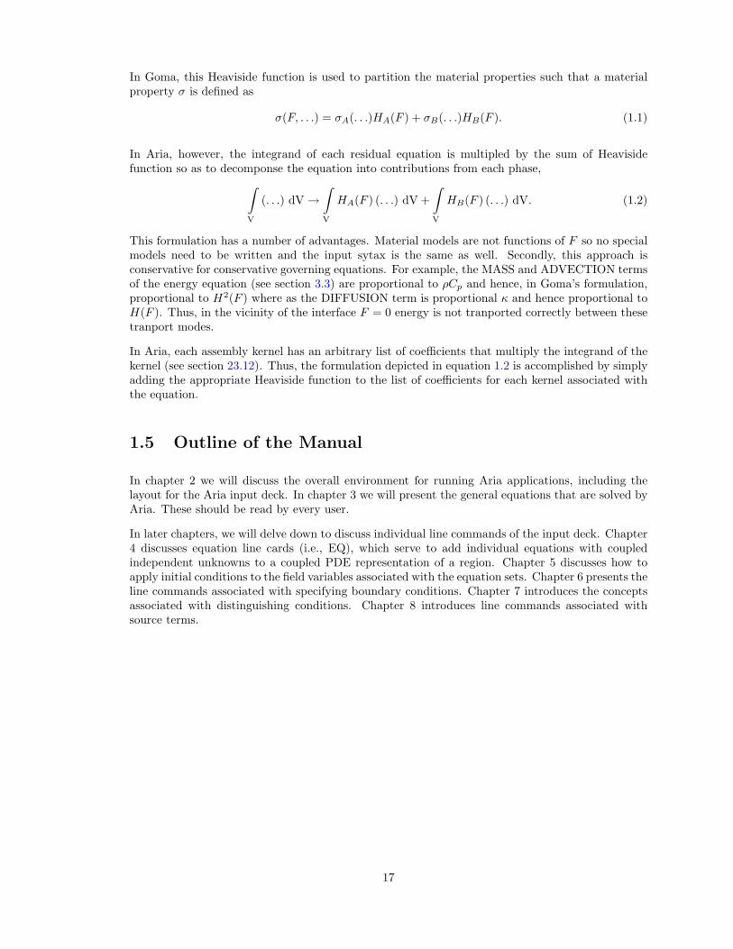
In Goma, this Heaviside function is used to partition the material properties such that a materialproperty σ is defined as
σ(F, . . .) = σA(. . .)HA(F ) + σB(. . .)HB(F ). (1.1)
In Aria, however, the integrand of each residual equation is multipled by the sum of Heavisidefunction so as to decomponse the equation into contributions from each phase,∫
V
(. . .) dV →∫V
HA(F ) (. . .) dV +∫V
HB(F ) (. . .) dV. (1.2)
This formulation has a number of advantages. Material models are not functions of F so no specialmodels need to be written and the input sytax is the same as well. Secondly, this approach isconservative for conservative governing equations. For example, the MASS and ADVECTION termsof the energy equation (see section 3.3) are proportional to ρCp and hence, in Goma’s formulation,proportional to H2(F ) where as the DIFFUSION term is proportional κ and hence proportional toH(F ). Thus, in the vicinity of the interface F = 0 energy is not tranported correctly between thesetranport modes.
In Aria, each assembly kernel has an arbitrary list of coefficients that multiply the integrand of thekernel (see section 23.12). Thus, the formulation depicted in equation 1.2 is accomplished by simplyadding the appropriate Heaviside function to the list of coefficients for each kernel associated withthe equation.
1.5 Outline of the Manual
In chapter 2 we will discuss the overall environment for running Aria applications, including thelayout for the Aria input deck. In chapter 3 we will present the general equations that are solved byAria. These should be read by every user.
In later chapters, we will delve down to discuss individual line commands of the input deck. Chapter4 discusses equation line cards (i.e., EQ), which serve to add individual equations with coupledindependent unknowns to a coupled PDE representation of a region. Chapter 5 discusses how toapply initial conditions to the field variables associated with the equation sets. Chapter 6 presents theline commands associated with specifying boundary conditions. Chapter 7 introduces the conceptsassociated with distinguishing conditions. Chapter 8 introduces line commands associated withsource terms.
17

18
Chapter 2
Getting Started
2.1 Setting Up Your Environment
To access Sierra/Aria/Arpeggio one additional entry to your path, the location of the SNToolsdirectory, is required. The SNTools team maintains installations on most of the compute resourcesavailable to Sandians and sometimes those change from machine to machine. See The SNToolsProject for more details about running on specialized machines. On many machines, including theLinux desktops on the 9100 LAN, the path is that shown in this example.
In addition to setting up your path (see below) you should verify that you are using Sandia’s versionof ssh that includes Kerberos authentication support so that you can run parallel jobs withouthaving to supply your password for each additional process spawned by mpi.
2.1.1 Setting up for the csh and tcsh Shells
Add SNTools to your path. In either your /.cshrc or /.tcshrc file add the line
set path=(/home/sntools/production/current/sntools/engine $path)
2.1.2 Setting up for the bash Shell
Add SNTools to your path. In either your /.bashrc or /.profile file add the line
export PATH=/home/sntools/production/current/sntools/engine:$PATH
2.2 Running Aria
This section includes some very simple examples of how to run Aria. For more information onrunning on some of Sandia’s clusters, etc. see The SNTools Project.
In its simplest form, Aria can be run like this:
% sierra aria -i ariarun.i
In this example, ariarun.i is the Aria input file. The output – nonlinear iterations, time stepinformation, etc. – will be written to a file called ariarun.log. So, you can monitor the progressof the simulation by watching the log file. Alternatively, you can have all of the output sent to
19
the screen by using the -l logfile command line option. If you set the log file to be - (a single“minus” character) all of the output will be sent to the standard output (usually your screen):
% sierra aria -i ariarun.i -l -
If you would like to use aprepro in your input file, add the -a command line option to have yourinput file automatically processed:
% sierra aria -i ariarun.i -l - -a
Oftentimes we want to run Aria remotely or locally in a batch mode, save any standard outputand perhaps even logout from a session. Unfortunately, termination of the session through eithervoluntary (interactive) or involuntary (timeout) logout out may in effect terminate the Aria job. Inthis caes one can prevent the job from terminating by using the Unix nohup command in conjunctionwith the standard execution command line.
% nohup sierra aria -i ariarun.i -l YourLogFile -a
2.3 Aria Environment Overview
Aria is a Sierra application implementing the finite element method (FEM) for solving systemsof partial differential equations (PDEs). Foremost, Aria’s development targets applications whichinvolve incompressible flow (Navier-Stokes). However, the general design of Aria lends itself tothe solution of systems of PDEs describing physical processes including energy transport, speciestranport with reactions, electrostatics and general transport of scalar, vector and tensor quantitiesin two and three dimensions both transient and direct to steady state. Moreover, different regionsof the physical domain (i.e., the input mesh) may have either different materials and/or differentcollections of physics (viz., PDEs) defined on them. These systems of equations may be solvedalone, in a segregated but coupled algorith (“loosely coupled”) or as a single, fully-coupled system.Currently, Aria’s loose coupling capabilities are handled by the Arpeggio application which alsoallows Aria to couple (loosely) to the quasistatic structural mechanics code, Adagio.
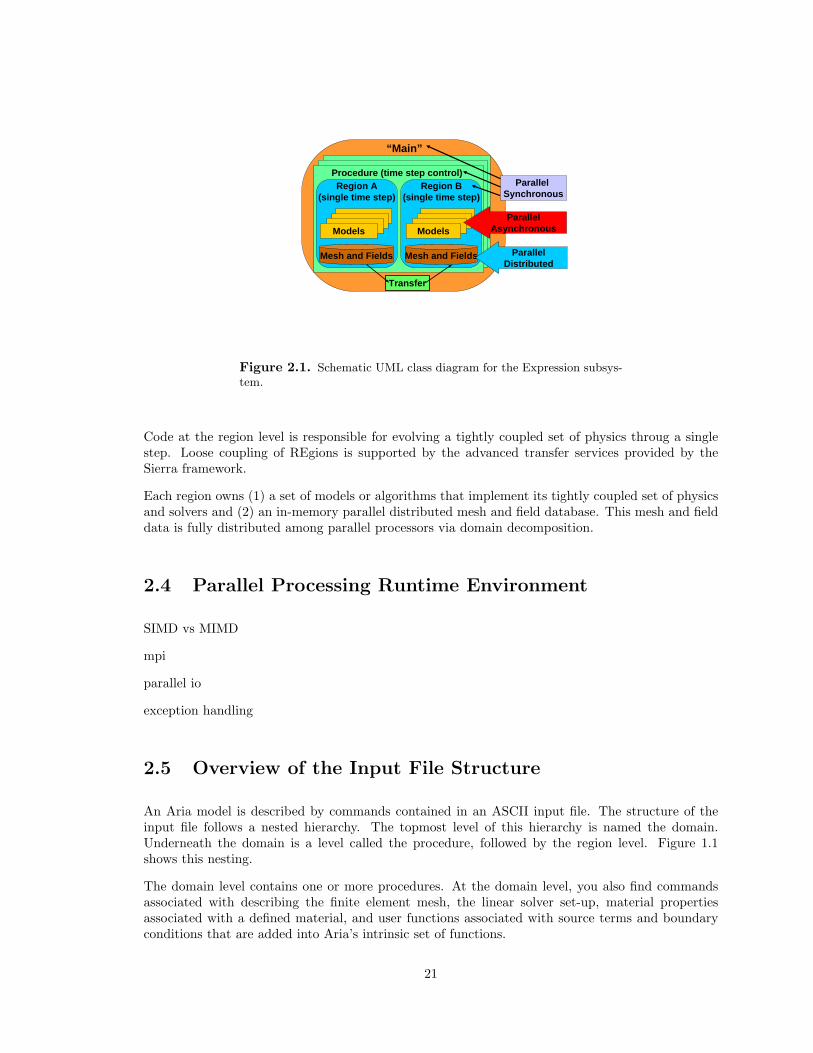
Aria’s models and algorithms are integrated into the Sierra framework through the architectureillustrated in Figure 2.1. A Sierra-based application has four layers of code: Domain, Procedure,Region, and Model/Algorithm.
The outermost layer of an application is the Domain, or “main” program of the application. THisdomain layer is implemented by the Sierra Framework to manage the startup/shutdown of an ap-plication, and to orchestrate the execution of an application-proved set of procedures.
Code at the Procedure level is rsponsible for evolving one or more s loosely coupled ses of physicsthrough a sequence of steps. This sequence may be a set of time steps, nonlinear solver iterations,or some combinations of these or other types of steps.
An application mauy define multiple procedures to implement hand-off coupling between physicswithin the same main program. In hand-off coupling the first (or preceding) procedure completesexecution, mesh and field data is transferred to a succeeding procedure, and the succeeding procedurecontinues the simulation with a different set of physics. For example, the first thermal procedurecould calculate a temperature distribution inside a differentially heated fluid, and the second pro-cedure could simulate natural convection of the fluid due to the density gradients set up by theresulting temperature field.
20
“Main”
Procedure (time step control)Region A
(single time step)
Models
Mesh and Fields
Region B(single time step)
Models
Mesh and Fields
Transfer
Parallel Synchronous
ParallelAsynchronous
ParallelDistributed
Figure 2.1. Schematic UML class diagram for the Expression subsys-tem.
Code at the region level is responsible for evolving a tightly coupled set of physics throug a singlestep. Loose coupling of REgions is supported by the advanced transfer services provided by theSierra framework.
Each region owns (1) a set of models or algorithms that implement its tightly coupled set of physicsand solvers and (2) an in-memory parallel distributed mesh and field database. This mesh and fielddata is fully distributed among parallel processors via domain decomposition.
2.4 Parallel Processing Runtime Environment
SIMD vs MIMD
mpi
parallel io
exception handling
2.5 Overview of the Input File Structure
An Aria model is described by commands contained in an ASCII input file. The structure of theinput file follows a nested hierarchy. The topmost level of this hierarchy is named the domain.Underneath the domain is a level called the procedure, followed by the region level. Figure 1.1shows this nesting.
The domain level contains one or more procedures. At the domain level, you also find commandsassociated with describing the finite element mesh, the linear solver set-up, material propertiesassociated with a defined material, and user functions associated with source terms and boundaryconditions that are added into Aria’s intrinsic set of functions.
21
The procedure level contains one or more regions. The procedure level is also used to specify thetime stepping parameters, and interactions between regions, such as data transfers. Essentially atthe procedure level, loose coupling algorithms are specified. Loose coupling here is defined within thecontext of Aria’s implicitly full-coupled paradigm. Whenever an independent variables’s interactionwith other variables in the solution procedure is not fully represented in the global matrix, thealgorithm for loose coupling of that variable and its associated equation will be described at theprocedure level. This loose coupling algorithm is given a fancy name called a “solution controldescription”. The procedure level contains a block specifying the solution control procedure. Ananalogy to this block in simpler codes would be top level loop. For example in time dependentapplications, the solution control description block would involve a block to solve the time dependentproblem repeated for each time step until the desired solution time is reached.
The region level is used to specify details about the tightly coupled equation system to be solved. Thedetails include boundary conditions and initial conditions, where materials models are applied, andwhere surface and volumetric source terms are applied. Essentially, meshes and material propertiesdescribed at the domain level are tied into the problem statement here via their names.
Global constraints equations are also specified at the region level. At the region level, specificationof what gets sent to the output file and at what frequency also is made. Additional post-processingassociated with the output is specified. For example, additional volumetric fields which are functionsof the independent variables may be specified to be added to the output file.
There are two types of commands in the input file. The first type is referred to as a block command.A block command is a grouping mechanism. A block command contains a set of commands madeup of other block commands and line commands. A line command is the second type of command.The domain, procedure, and region levels are all parsed as block commands. A block command isdefined in the input file by a matching pair of Begin and End lines. For example,
Begin SIERRA myJob
.....
End SIERRA myJob
A set of key words for the block command follows the “Begin” and “End” keywords. In most cases auser-specified name is added to the block commands. In the example above the keywords, SIERRAmyJob, are added. Optionally, the keyword may be left off of the end of the block.
The second type of command is the line command. A line command is used to specify parameterswithin a given block command. In the remaining chapters and sections of this manual, the scope ofeach block and line command is identified, along with summaries of the meanings. Note that theordering of any commands within a command block is arbitrary. Thus,
Begin Finite Element model fluid
Database name is pipeflow2d.g
Use Material water for block1
End Finite Element model fluid
will have the same effect as
Begin Finite Element model fluid
Use Material water for block1
Database name is pipeflow2d.g
22
End Finite Element model fluid
And the ordering of command blocks within the domain/procedure/region blocks are arbitrary–allowing you conderable freedom to collect and arrange commands. Note that the terms “commandblock” and “block command” are interchangeable.
The sierra command block must contain a block for a procedure containing an aria region:
Begin procedure myProcedureName
Begin Aria region name
End Aria region name
End procedure myProcedureName
The procedure command block is used to contain all of the Aria commands that are associated witha solution procedure defined for a set of Aria Regions. The myProcedureName and name keywordsof the procedure and region blocks are left up to you. Note that the Aria procedure commandblock must be present in the input file and must contain at least one Aria region command block.The procedure command block also contains other important command blocks such as the TIMESTEPPING block.
2.5.1 Syntax Conventions for Commands
In this section we describe the conventions used in presenting all the command descriptions in theremainder of this manual. There are four basic kinds of tokens, or words, that Aria expects to findas it parses an input file. These are keywords, names, parameters and delimiters.
2.5.1.1 Keywords
The words which distinguish one block command, or line command, from another we term keywords.Keywords are denoted in this manual in the monospaced font, for example, BOUNDARY CONDITION.
2.5.1.2 Names
The word, or words, that you supply on the same line of the begin line of a block command, is thename. Many times you may need to supply this name as a character parameter in a separate linecommand. Names are denoted in italics, name , as are parameters.
2.5.1.3 Parameters
There are three types of input parameters you may need to supply to line commands: characterstrings, integers, and real numbers. These are denoted in the documentation as (C), (I), and (R),respectively. Character strings don’t have to be delimited by quotation marks. Real numbers may beentered in decimal form or exponential form. For example 0.0001, .1E-3, 10.0d-5 are all equivalent.Furthermore, if a real(R) is expected, an integer can be used. If an integer(I) is expected, however,you must specify it without a decimal point.
23
2.5.1.4 Multiple Parameters
For the case when a list of one or more paremeters is allowed, or required, for a command, (C,...)denotes a list of character strings, (I,...) a list of integers, and (R, ...) a list of real numbers. Fora list of character strings, the separator between the strings must be one or more spaces or tabcharacters. Therefore, phrases with multiple spaces and words in them are tokenized into multiplecharacter parameters before being processed by the application. For a list of real or integer numbersthe comma can also be used as a separator.
2.5.1.5 Enumerated Parameters
Certain commands have predefined parameters, called enumerations, which are listed within .Each parameter in the list is separated using | . The default parameter for the list of parameters isenclosed by <>.
2.5.1.6 Delimiters
The keywords of a line command are often required to be separated from the parameters by adelimiter. You have a choice of delimiters to use: the equal sign, =, or a word. In this manual, wedenote the choices surrounded by , and separated by |. You may use any one of the delimiters fromthose listed. For example, the line command to specify the density within the Property Specificaitonfor Material Block command is
Density = |IS (R)
Examples of valid form syou could write in the input file are
Begin Property Specificaiton for Material water ... Density 1.0E-3 # kg/m3 at 20C ... End
and
Examples of valid form syou could write in the input file are
Begin Property Specificaiton for Material water ... Density is 1.0E-3 # kg/m3 at 20C ... End
2.5.1.7 White Space
Command keywords, names, and parameters and delimiters must have spaces around them.
2.5.1.8 Indentation
All leading spaces and/or tab characters are ignored in the input file. Of course, we recommendthat you use indentation to improve the readability for yourself and others that may need to seeyour files.
2.5.1.9 Case Sensitivity
None of the command keywords, parameters, or delimiters read from the input file are case sensitive.For example, the following two lines are equivalent:
24
Use Material water for block_1
and
USE material wATer for blOCK_1
The exception to this rule are file names used for input and output, because the current operatingsystems on which SIERRA applications are run are based on UNIX, where file names are casesensitive.
2.5.1.10 Comments and Line Continuation
You may place comments in the input file starting with either the $ or # character. All furthercharacters on al ine following a comment character are ignored.
You can continue a command in the input file to the next line by using the line continuation character$, or you may optionally following it with a comment#. All further characters on the same linefollowing a line continuation character $ are ignored, and the characters on the following line arejoined and parsing continues. An example is the line command used to specify the title of a thermalmodel:
Begin SIERRA Job Indentifier
#
$ This thermal model for Aria simulates a convective heat transfer
#
Title \$ The title command is used to set the analysis title
Convective heat transfer to a part. The analysis \#
makes use of conjugate heat transfer to account for \$
cooling of a part due to flowing water.
...
End SIERRA Job Indentifier
2.5.1.11 Checking the Syntax
Errors in the input deck can be checked by adding the command, “-check” to the aria commandline. For example,
sierra aria -check -i input.i
This command will print the code echo of the input deck and any syntax errors within it to thescreen.
25
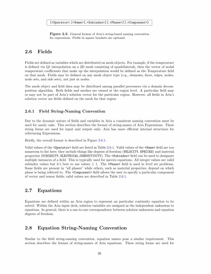
[<Operator> ]<Name>[ <Subindex>][ <Phase>][ <Component>]
Figure 2.2. General format of Aria’s string-based naming conventionfor expressions. Fields in square brackets are optional.
2.6 Fields
Fields are defined as variables which are distributed on mesh objects. For example, if the temperatureis defined via Q1 interpolation on a 2D mesh consisting of quadrilaterals, then the vector of nodaltemperature coefficients that make up the interpolation would be defined as the Temperature fieldon that mesh. Fields may be defined on any mesh object type (e.g., elements, faces, edges, nodes,node sets, and side sets), not just at nodes.
The mesh object and field data may be distribued among parallel processors via a domain decom-position algorithm. Both fields and meshes are owned at the region level. A particular field mayor may not be part of Aria’s solution vector for the particular region. However, all fields in Aria’ssolution vector are fields defined on the mesh for that region.
2.6.1 Field String-Naming Convention
Due to the dynamic nature of fields and variables in Aria a consistent naming convention must beused for sanity sake. This section describes the format of string-names of Aria Expressions. Thesestring forms are used for input and output only; Aria has more efficient internal structures forreferencing Expressions.
Briefly, the overall format is described in Figure 2.6.1.
Valid values of the <Operator> field are listed in Table 2.6.1. Valid values of the <Name> field are toonumerous to list here; they include things like degrees of freedom (VELOCITY, SPECIES) and materialproperties (VISCOSITY, ELECTRICAL CONDUCTIVITY). The <Subindex> field can be used to designatemultiple instances of a field. This is typically used for species equations. All integer values are validsubindex values but it’s best to use values ≥ 1. The <Phase> field is used in level set problems.Some fields are present in “all phases” while others, such as material properties, depend on whichphase is being referred to. The <Component> field allows the user to specify a particular componentof vector and tensor fields; valid values are described in Table 2.6.1.
2.7 Equations
Equations are defined within an Aria region to represent an particular continuity equation to besolved. Within the Aria input deck, solution variables are assigned as the independent unknowns toequations. In general, there is a one-to-one correspondence between solution unknowns and equationdegrees of freedom.
2.8 Equation String-Naming Convention
Similar to the field string-naming convention, equation names pose a similar requirement. Thissection describes the format of string-names of Aria equations. These string forms are used for
26
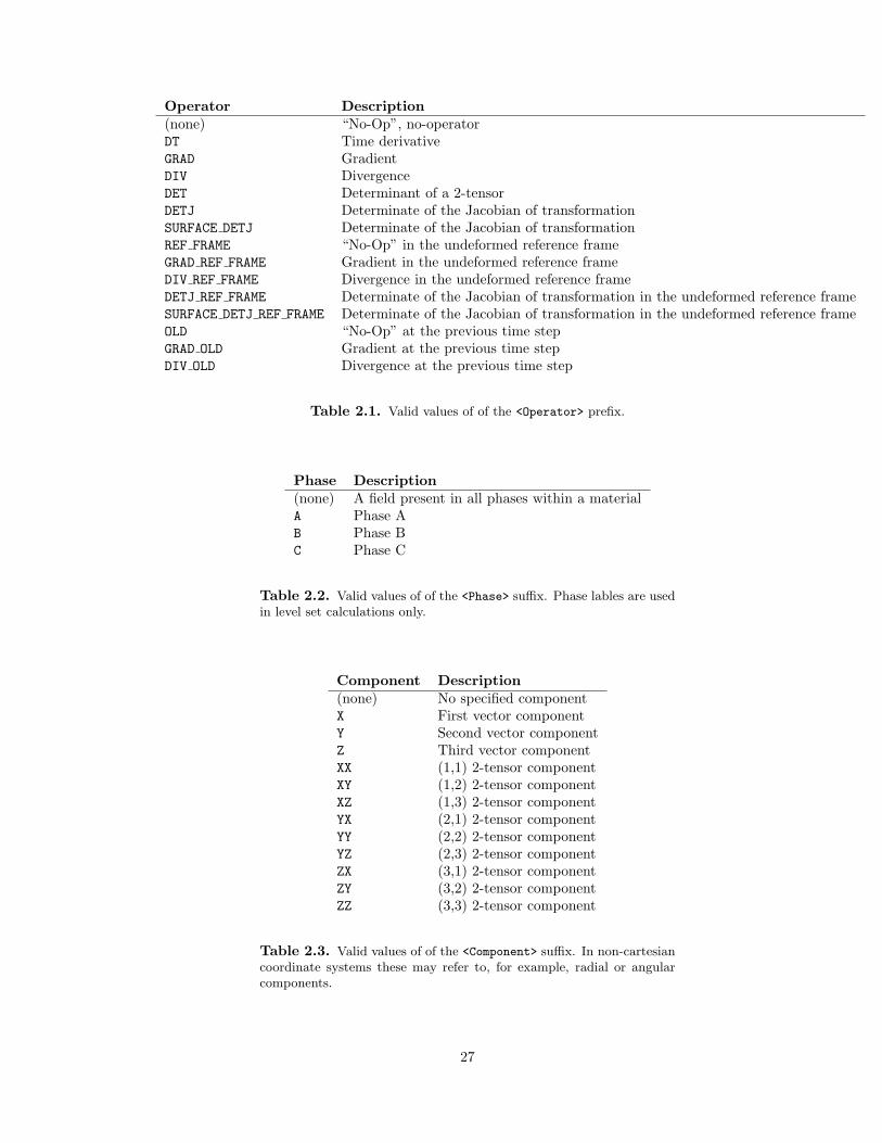
Operator Description(none) “No-Op”, no-operatorDT Time derivativeGRAD GradientDIV DivergenceDET Determinant of a 2-tensorDETJ Determinate of the Jacobian of transformationSURFACE DETJ Determinate of the Jacobian of transformationREF FRAME “No-Op” in the undeformed reference frameGRAD REF FRAME Gradient in the undeformed reference frameDIV REF FRAME Divergence in the undeformed reference frameDETJ REF FRAME Determinate of the Jacobian of transformation in the undeformed reference frameSURFACE DETJ REF FRAME Determinate of the Jacobian of transformation in the undeformed reference frameOLD “No-Op” at the previous time stepGRAD OLD Gradient at the previous time stepDIV OLD Divergence at the previous time step
Table 2.1. Valid values of of the <Operator> prefix.
Phase Description(none) A field present in all phases within a materialA Phase AB Phase BC Phase C
Table 2.2. Valid values of of the <Phase> suffix. Phase lables are usedin level set calculations only.
Component Description(none) No specified componentX First vector componentY Second vector componentZ Third vector componentXX (1,1) 2-tensor componentXY (1,2) 2-tensor componentXZ (1,3) 2-tensor componentYX (2,1) 2-tensor componentYY (2,2) 2-tensor componentYZ (2,3) 2-tensor componentZX (3,1) 2-tensor componentZY (3,2) 2-tensor componentZZ (3,3) 2-tensor component
Table 2.3. Valid values of of the <Component> suffix. In non-cartesiancoordinate systems these may refer to, for example, radial or angularcomponents.
27
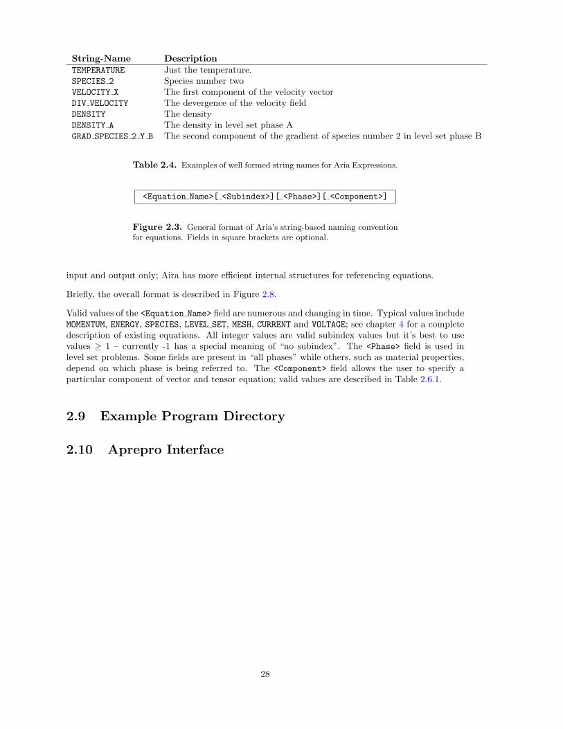
String-Name DescriptionTEMPERATURE Just the temperature.SPECIES 2 Species number twoVELOCITY X The first component of the velocity vectorDIV VELOCITY The devergence of the velocity fieldDENSITY The densityDENSITY A The density in level set phase AGRAD SPECIES 2 Y B The second component of the gradient of species number 2 in level set phase B
Table 2.4. Examples of well formed string names for Aria Expressions.
<Equation Name>[ <Subindex>][ <Phase>][ <Component>]
Figure 2.3. General format of Aria’s string-based naming conventionfor equations. Fields in square brackets are optional.
input and output only; Aira has more efficient internal structures for referencing equations.
Briefly, the overall format is described in Figure 2.8.
Valid values of the <Equation Name> field are numerous and changing in time. Typical values includeMOMENTUM, ENERGY, SPECIES, LEVEL SET, MESH, CURRENT and VOLTAGE; see chapter 4 for a completedescription of existing equations. All integer values are valid subindex values but it’s best to usevalues ≥ 1 – currently -1 has a special meaning of “no subindex”. The <Phase> field is used inlevel set problems. Some fields are present in “all phases” while others, such as material properties,depend on which phase is being referred to. The <Component> field allows the user to specify aparticular component of vector and tensor equation; valid values are described in Table 2.6.1.
2.9 Example Program Directory
2.10 Aprepro Interface
28
Chapter 3
Equations Aria Solves
3.1 Generalized Conservation Equation
We first introduce a general conservation equation, as a model for the specific equations that Ariasolves, demonstrating how the galerkin finite element method is applied to it, and how the integra-tion by parts is carried out on its individual terms. Following Deen (1998), the conservation of ageneral scalar quantity b(x, t), with units of amount-per-unit-volume, at a point x and time t canbe expressed as
∂b
∂t+ ∇ · (bv) = −∇ · f + BV (3.1)
where v is the mass average velocity, f is the diffusive flux of b, and BV is the volumetric source ofb.
The Galerkin FEM (G/FEM) residual form of 3.1 is formed by bringing the right hand side termsto the left, multiplying by the FEM weight function φi and integrating over the volume V,
Rib =
∫V
(∂b
∂t+ v · ∇b + b∇ · v + ∇ · f −BV
)φi dV = 0. (3.2)
In many applications ∇·v = 0 so we ignore that term from here on. However, it is straight forward toaccount for this term via the source term BV. Using the vector identity (∇·f)φi = ∇·(fφi)−∇φi ·fand using the divergence theorem, 3.2 becomes
Rib =
∫V
[(∂b
∂t+ v · ∇b−BV
)φi −∇φi · f
]dV +
∫S
n · fφi dS = 0. (3.3)
Here n is a unit normal along the boundary S, pointing out of the volume V.
Equation 3.3 embodies the sign convention for sources, fluxes and equation terms used within Aria.For example, scalar flux expressions in Aria provide values for fn ≡ n · f and should be positive fora flux of b leaving the volume V.
Note also that we have not assigned a units convention to the equation. Any unit system may beemployed in the specification of the individual terms in 3.1. However, each term in 3.1 must haveoverall units of [b] / [time], and the overall residual expression has units of [b] * [L]**3 / [time],where [b] are units of the conserved quantity, b, [L] is the unit of the length scale, and [time] is theunit for time.
3.2 Conservation of Mass
For a material with density ρ, letting b = ρ results in the conservation of mass. Since there is nonet flow relative to the mass average velocity f = 0. Although there are no sources of mass, having
29
such a source can be convenient in modeling and simulation; so, we let the mass source be BV = qm.Thus, (3.1) becomes
∂ρ
∂t+ ρ∇ · v + v · ∇ρ = qm. (3.4)
For the special but common case of constant density, this reduces to
∇ · v = 0. (3.5)
Using equation 3.3, the G/FEM residual form is
RiP =
∫V
(−∂ρ
∂t− ρ∇ · v − v · ∇ρ + qm
)φi dV = 0. (3.6)
Important Note: Equation 3.6 has been multiplied by -1 because this form results in a better linearsystem for the special case of incompressible flow. This is important to remember when definingmass source terms.
In Aria, each term in 3.6 is specified separately as identified in equation 3.7.
RiP =
∫V
−∂ρ
∂tφi dV
︸ ︷︷ ︸MASS
+∫V
− (v · ∇ρ + ρ∇ · v) φi dV
︸ ︷︷ ︸ADV
+∫V
qmφi dV
︸ ︷︷ ︸SRC
= 0 (3.7)
For a purely incompressible form, Aria offers the alternative form given in 3.8;
RiP +
∫V
−∇ · vφi dV
︸ ︷︷ ︸DIV
+∫V
qmφi dV
︸ ︷︷ ︸SRC
= 0 (3.8)
3.3 Conservation of Energy
For a material with constant density and specific heat Cp, temperature T , heat flux q and volumetricenergy source HV , letting b = ρCpT , f = q and BV = HV results in the conservation of energy.
ρCp∂T
∂t+ ρCpv · ∇T = −∇ · q + HV . (3.9)
A common constitutive relationship for q is Fourier’s law, q = −κ∇T where κ is the thermalconductivity. However, we leave the heat flux as an option to be specified as part of the materialproperties (see section 10.13). Using equation 3.3, the G/FEM residual form is
RiT =
∫V
[(ρCp
∂T
∂t+ ρCpv · ∇T −HV
)φi −∇φi · q
]dV +
∫S
qnφi dS = 0 (3.10)
where qn is the heat flux at the boundary. For example, the natural convection boundary conditiongives qn = h(T − T∞) where h is the heat transfer coefficient and T∞ is the bulk temperature awayfrom the surface.
30
In Aria, each term in 3.10 is specified separately as identified in equation 3.11.
RiT =
∫V
ρCp∂T
∂tφi dV
︸ ︷︷ ︸MASS
+∫V
ρCpv · ∇Tφi dV
︸ ︷︷ ︸ADV
−∫V
HV φi dV
︸ ︷︷ ︸SRC
−∫V
∇φi · q dV
︸ ︷︷ ︸DIFF
+∫S
qnφi dS = 0 (3.11)
More and more often we needing to account for variable density problems and so we need to bringback some of the terms we threw away because we were going to assume ∇·v ≡ 0. Here’s a do-overof equation 3.11 that accomodates a variable density through the DIV term:
RiT =
∫V
ρCp∂T
∂tφi dV
︸ ︷︷ ︸MASS
+∫V
ρCpv · ∇Tφi dV
︸ ︷︷ ︸ADV
+∫V
ρCpT∇ · vφi dV
︸ ︷︷ ︸DIV
−∫V
HV φi dV
︸ ︷︷ ︸SRC
−∫V
∇φi · q dV
︸ ︷︷ ︸DIFF
+∫S
qnφi dS = 0 (3.12)
Note, however, that equation 3.12 still assumes a constant specific heat Cp.
3.4 Conservation of Chemical Species
For a material with species k with molar concentration Ck, molar flux Jk relative to the mass averagevelocity and volumetic reation rate RV,k, letting b = yk, f = Jk and BV = RV,k in (3.1) results inthe conservation equation for species k,
∂Ck
∂t+ v · ∇Ck = −∇ · Jk + RV,k. (3.13)
For liquid mixtures which are dilute in all species except one, Fick’s law is often used to approximateJk. In this approximation, Dk represents the diffusion coefficient of species k with respect to theconcentrated species and it is assumed that the interactions between dilute species is assumednegligible. Again, however, we choose to leave the governing equation in the more general form andrequire the particular diffusive flux model as user input (see section 10.30). Using equation 3.3, theG/FEM residual form is
RiCk
=∫V
[(∂Ck
∂t+ v · ∇Ck −RV,k
)φi −∇φi · Jk
]dV +
∫S
qn,kφi dS = 0 (3.14)
where qn,k is the mass flux at the boundary. For example, the natural convection boundary conditiongives qn = k(Ck −C∞,k) where k is the mass transfer coefficient and C∞,k is the bulk concentrationaway from the surface.
31
In Aria, each term in 3.14 is specified separately as identified in equation 3.15.
RiCk
=∫V
∂Ck
∂tφi dV
︸ ︷︷ ︸MASS
+∫V
v · ∇Ckφi dV
︸ ︷︷ ︸ADV
−∫V
RV,kφi dV
︸ ︷︷ ︸SRC
−∫V
∇φi · Jk dV
︸ ︷︷ ︸DIFF
+∫S
qn,kφi dS = 0 (3.15)
More and more often we needing to account for variable density problems and so we need to bringback some of the terms we threw away because we were going to assume ∇·v ≡ 0. Here’s a do-overof equation 3.15 that accomodates a variable density through the DIV term:
RiCk
=∫V
∂Ck
∂tφi dV
︸ ︷︷ ︸MASS
+∫V
v · ∇Ckφi dV
︸ ︷︷ ︸ADV
+∫V
C∇ · vφi dV
︸ ︷︷ ︸DIV
−∫V
RV,kφi dV
︸ ︷︷ ︸SRC
−∫V
∇φi · Jk dV
︸ ︷︷ ︸DIFF
+∫S
qn,kφi dS = 0 (3.16)
Often times it is useful to solve for mass, weight or volume fractions of each species rather than forthe concentration directly. In that case, an additional condition exists,∑
k
Ck = 1 (3.17)
Using this condition, it is only necessary to solve for N − 1 species fractions where N is the totalnumber of species present in the problem. The final species, then, is simply given as
Cj = 1−∑k 6=j
Ck (3.18)
This method can be triggered in Aria by specifing the equation term FRACBAL. In this case, theequation for Cj is not included in the system of unknowns but is instead post-processed on the fly.Aria will automatically detect all other species equations and include them in the fraction balance.
3.5 Conservation of Fluid Momentum
The Cauchy momentum equation is given by
ρ∂v
∂t+ ρv · ∇v − g −∇ · T = 0 (3.19)
where T is the fluid stress tensor and g is a body force. We construct the G/FEM residual formof 3.19 by contracting with the unit coordinate vector in the k-direction, ek, multiplying by theweight function φi and integrating over the volume. Using the vector identiy (∇ · T ) · ekφi =∇ · (T · ekφi)− T t : ∇(ekφi) and integrating by parts gives
Rim,k =
∫V
[(ρ∂v
∂t+ ρv · ∇v − g
)· ekφi + T t : ∇
(ekφi
)]dV −
∫S
n · T · ekφi dS = 0 (3.20)
32
In Aria, each term in 3.20 is specified separately as identified in equation 3.15.
Rim,k =
∫V
ρ∂v
∂t· ekφi dV
︸ ︷︷ ︸MASS
+∫V
ρv · ∇v · ekφi dV
︸ ︷︷ ︸ADV
−∫V
g · ekφi dV
︸ ︷︷ ︸SRC
+∫V
T t : ∇(ekφi
)dV
︸ ︷︷ ︸DIFF
−∫S
n · T · ekφi dS = 0 (3.21)
3.6 Conservation of Solid Momentum
Aria currently solves the quasistatic form of the solid momentum equations. Furthermore, the solidstress is treated as a linear elastic material. In this limit, the Cauchy momentum equation is givenby
∇ · T = 0 (3.22)
where T is the solid stress tensor. We construct the G/FEM residual form of 3.19 by contractingwith the unit coordinate vector in the k-direction, ek, multiplying by the weight function φi andintegrating over the volume. Using the vector identiy (∇ · T ) · ekφi = ∇ · (T · ekφi)−T t : ∇(ekφi)and integrating by parts gives
Rim,k =
∫V
T t : ∇(ekφi
)dV = 0 (3.23)
Here, the surface contribution,∫Sn · T · ekφi dS, has been dropped because Aria currently only
supports dirichlet and natural (homogeneous) boundary conditions for the solid equation.
In Aria, each term in 3.23 is specified separately as identified in equation 3.24.
Rim,k =
∫V
T t : ∇(ekφi
)dV
︸ ︷︷ ︸DIFF
= 0 (3.24)
Currently, Aria does not support direct specification of the more popular stress-strain parametizationthat utilizes Young’s modulus E, Poisson’s ratio ν and coefficient of thermal expansion α (note, theshear modulus G = µ). The relationship between these two parametizations is summarized here forconvenience.
2µ =E
(1 + ν)(3.25)
λ =νE
(1 + ν) (1− 2ν)= 2µ
ν
(1− 2ν)(3.26)
β =αE
(1− 2ν)= α (3λ + 2µ) (3.27)
3.7 Voltage Equation
The electric potential or voltage V is frequently used in determining the electric field, E = −∇V .While (3.1) cannot be applied to the voltage, the equation governing the voltage – Gauss’ law from
33
Maxwell’s equations – has a similar form. Writing the electric displacement D as D = εE, where εis the electric permittivity, Gauss’ law is
∇ · ε∇V = ρe (3.28)
where the permittivity is taken to be a constant and ρe is the volumetric free charge density.
Using equation 3.3, the G/FEM residual form is
RiV =
∫V
(−ρeφ
i + ∇φi · ε∇V)
dV +∫S
qnφi dS = 0 (3.29)
In Aria, each term in 3.29 is specified separately as identified in equation 3.30.
RiV = −
∫V
ρeφi dV
︸ ︷︷ ︸SRC
+∫V
∇φi · ε∇V dV
︸ ︷︷ ︸DIFF
+∫S
qnφi dS = 0 (3.30)
3.8 Current Equation
An alternate formulation for solving for the electrical potential (see section 3.7) is to solve the“current” equation which is a conservation equation for electrical charge. The electrical current Jis frequently related to the electric field E using Ohm’s law as J = σeE where σe is the electricalconductivity. The electric potential or voltage V is used in determining the electric field, E = −∇V .However, we choose to leave the electrical current as a more general constitutive model to be providedas a material model input (see section 10.4).
−∇ · J = ρe (3.31)
Using equation 3.3, the G/FEM residual form is
RiV =
∫V
(−ρeφ
i −∇φi · J)
dV +∫S
qnφi dS = 0 (3.32)
In Aria, each term in 3.32 is specified separately as identified in equation 3.33.
RiV = −
∫V
ρeφi dV
︸ ︷︷ ︸SRC
−∫V
∇φi · J dV
︸ ︷︷ ︸DIFF
+∫S
qnφi dS = 0 (3.33)
3.9 Suspension Equation
In treating the suspension as a continuum, we introduce an evolution equation for particle volumefraction, φ, as
∂φ
∂t+ v · ∇φ + ∇ · N = 0. (3.34)
The particle volume fraction is defined as the total summed volume of particles per volume of theparticle medium. 3.34 represents a balance between the storred particles, the convected particle flux,
34
and the diffusive particle flux, N . Several mechanisms which include Brownian motion, sedimen-tation, hydrodynamic particle interactions, and gradients in suspension viscosity may contribute tothe diffusive particle flux. Specification of the appropriate flux model must then be carried out toclose the definition of the conservation equation.
3.10 Stress Tensor Projection Equation
A projection equation is defined as an equation where a derived quantity at the interior gausspoints is evaluated and projected to be a solution unknown at the nodal points. The stress tensorprojection equation projects the momentum stresses, tau, without the pressure term, to the nodalpoints. Projecting the momentum stress smoothes out the momentum stress tensor and allows for adot product to be carried out on the projected field, which is needed for least squares stabilizationschemes. The solution variable, τab, is calculated from 3.35.
RiV = −
∫V
(τab − src τab)φi dV
︸ ︷︷ ︸DEF
= 0 (3.35)
τab is a tensor variable. For 2D problems, ab stands for XX, XY, YX, and YY. For 3D problemsab stands for XX, XY, XZ, YX, YY, YZ, ZX, ZY, and ZZ. The source term in the equation srcτ ab
refers to the momentum stress without the pressure diagonal term.
src τxx = 2µdu
dx− 2
3(µ− λ)(∇ · v)
src τyy = 2µdv
dy− 2
3(µ− λ)(∇ · v)
src τzz = 2µdw
dz− 2
3(µ− λ)(∇ · v)
src τxy = src τyx = µ(du
dy+
dv
dx)
src τxz = src τzx = µ(du
dz+
dw
dx)
src τyz = src τzy = µ(dv
dz+
dw
dy)
35
3.11 Notes on Solid Mechanics
Some of the standard references on solid mechanics include Malvern (1969), Mase (1970), Bonetand Wood (1997) and Belytschko et al. (2004). As is often the case, the mathematical notion usedthrough-out these texts is different in many cases and this is often a source of confusion. Here, we’lllay out some basic defintions in our notation and, when possible, give the notation used in theseothere texts.
In what follows, x is the position vector of a material particle in the deformed or current spatialconfiguration and X is the position vector of a material particle in the undeformed or initial orreference configuration. The displacement vector d is the difference between these to states1 viz.x = X + d.
We will make extensive use of the gradients of these fields and so it is important to distinguishbetween gradients in the reference configuration and the current configuration. Gradients in thecurrent configuration are denoted ∇ in Gibbs notation or ∂ /∂xi in index notation. Gradients inthe reference configuration are denoted ∇X in Gibbs notation or ∂ /∂Xi in index notation2.
Next, we define the deformation gradient F
F ≡ ∇Xxt (3.36)= ∇XXt + ∇Xdt (3.37)= I + ∇Xdt (3.38)
where the superscript t denotes the transpose operator3. The inverse deformation gradient4, F−1,is also useful and can be computed as
F−1 ≡ ∇Xt (3.39)= ∇xt −∇dt (3.40)= I −∇dt. (3.41)
The determinants of F and F−1 are denoted J and J−1 respectively and are often used in transfor-mations between different stress definitions5.
It’s worth noting at this point that in Aria both gradient operators, ∇ and ∇X , are available asExpression objects as are F , F−1, J and J−1.
The Green or Green-Lagrange strain tensor E is defined6 as
E ≡ 12(F t · F − I
)(3.42)
=12(∇Xd + ∇Xdt + ∇Xd · ∇Xdt
). (3.43)
The Green strain is a strain measure in the reference configuration and is suitable for large defor-mations and large rotations. The analagous Eulerian (or Almansi’s) strain tensor E∗ is defined7
1d is denoted u in Malvern (1969), Mase (1970), Bonet and Wood (1997), and Belytschko et al. (2004).2In Belytschko et al. (2004) ∇X is denoted ∇0.3In Mase (1970) this is called the conjugate dyadic and is denoted with a subscript c. In Malvern (1969) the
quantity ∇Xxt is denoted x∇X where the arrow over the gradient operator denotes the direction of the operation.
4In Mase (1970) F−1 is denoted H.5Sometimes J is expressed as a ratio of the densities between the reference and current configurations, ρ/ρ.6In Mase (1970) E is denoted LG and is called the Lagrangian strain.7In Mase (1970) E∗ is denoted EA.
36
as
E∗ ≡ 12(I − F−t · F−1
)(3.44)
=12(∇d + ∇dt −∇d · ∇dt
). (3.45)
The Eulerian strain is also a suitable strain measure for large deformations and rotations but isdefined in the current configuration.
The Cauchy stress, σ, is a stress measure defined in the current configuration as
σ = λEkkI + 2µE (3.46)
where Ekk denotes the trace of E and λ and µ are the Lame coefficients. This constitutive equationmay also be augmented with some initial residual stress or a thermal stress,
σ = λEkkI + 2µE − β (T − T) I + σr. (3.47)
Here β is related to the coefficient of thermal expansion, T is the temperature, T is the referencetemperature of the solid and σr is the residual stress.
For large deformations and large rotations Aria uses the second Piola-Kirchhoff stress which isdefined in the reference configuration and is related to the Cauchy stress as
S = JF−1 · σ · F−t. (3.48)
The reverse transformation is readily given by
σ = J−1F · S · F t. (3.49)
Mathematically, the Cauchy stress σ is most conveniently expressed in terms of the Lame coefficientsλ, µ and β. In practice, however, it is more common to measure and report a different but related setof parameters: the Young’s modulus E, the Poisson’s ratio ν and the coefficient of thermal expansionα. (Note, the shear modulus G = µ.) The relationship between these two sets of parameters is
2µ =E
(1 + ν)(3.50)
λ =νE
(1 + ν) (1− 2ν)= 2µ
ν
(1− 2ν)(3.51)
β =αE
(1− 2ν)= α (3λ + 2µ) (3.52)
In Aria, there are separate Expression Names for the Cauchy stress and the second Piola-Kirchhoffstress expressions. In the input files, users provide their choice of constitutive relations in thematerial model specification, e.g.,
Begin Aria Material The_MaterialDensity = Constant rho = 2.33e-15Lambda = Constant lambda = 52810.30445Two Mu = Constant two_mu = 134426.2295Mesh Stress = Nonlinear_Elastic Reference_Frame=MovingMesh Stress = Residual Sx=-11 Sy=-11Mesh Stress = Isothermal T=800 T_ref=450
End
37
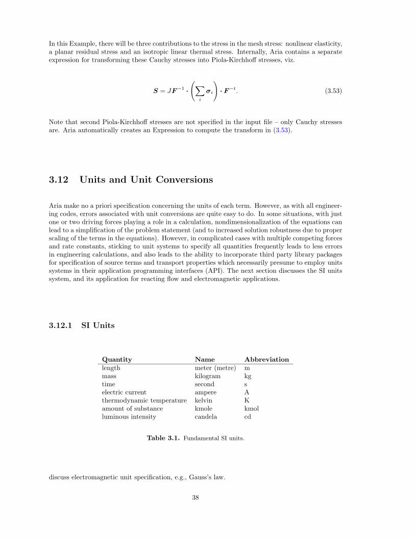
In this Example, there will be three contributions to the stress in the mesh stress: nonlinear elasticity,a planar residual stress and an isotropic linear thermal stress. Internally, Aria contains a separateexpression for transforming these Cauchy stresses into Piola-Kirchhoff stresses, viz.
S = JF−1 ·(∑
i
σi
)· F−t. (3.53)
Note that second Piola-Kirchhoff stresses are not specified in the input file – only Cauchy stressesare. Aria automatically creates an Expression to compute the transform in (3.53).
3.12 Units and Unit Conversions
Aria make no a priori specification concerning the units of each term. However, as with all engineer-ing codes, errors associated with unit conversions are quite easy to do. In some situations, with justone or two driving forces playing a role in a calculation, nondimensionalization of the equations canlead to a simplification of the problem statement (and to increased solution robustness due to properscaling of the terms in the equations). However, in complicated cases with multiple competing forcesand rate constants, sticking to unit systems to specify all quantities frequently leads to less errorsin engineering calculations, and also leads to the ability to incorporate third party library packagesfor specification of source terms and transport properties which necessarily presume to employ unitssystems in their application programming interfaces (API). The next section discusses the SI unitssystem, and its application for reacting flow and electromagnetic applications.
3.12.1 SI Units
Quantity Name Abbreviationlength meter (metre) mmass kilogram kgtime second selectric current ampere Athermodynamic temperature kelvin Kamount of substance kmole kmolluminous intensity candela cd
Table 3.1. Fundamental SI units.
discuss electromagnetic unit specification, e.g., Gauss’s law.
38
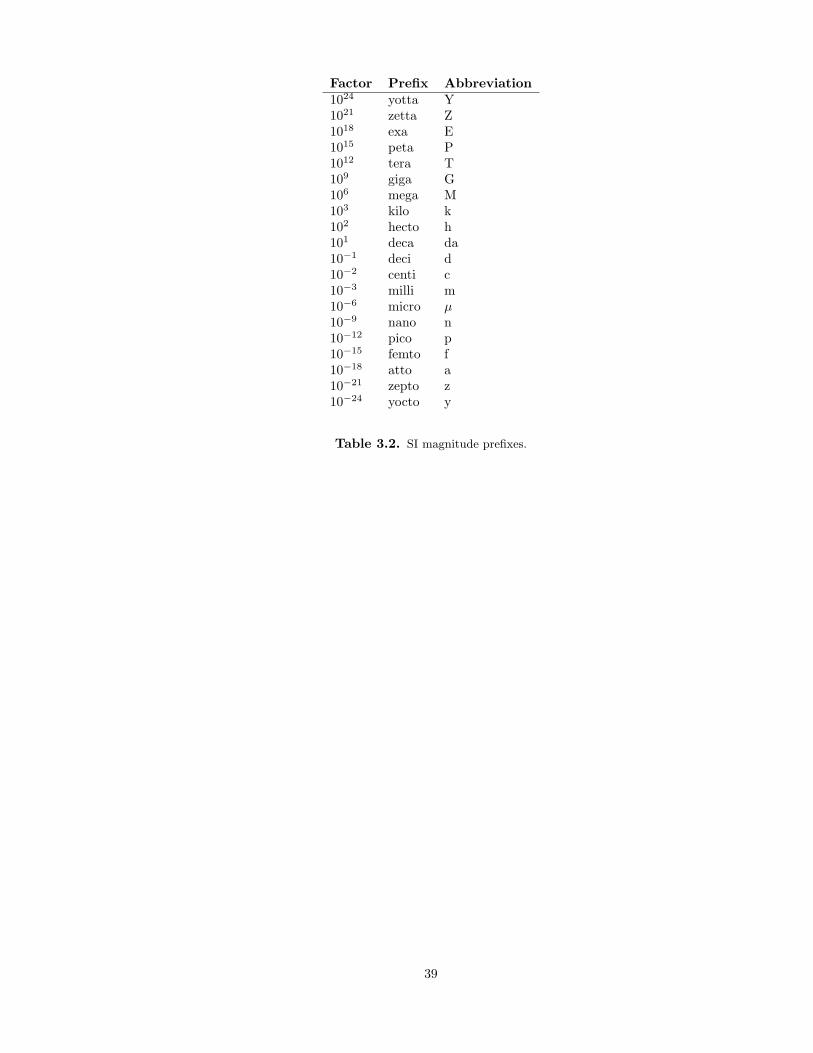
Factor Prefix Abbreviation1024 yotta Y1021 zetta Z1018 exa E1015 peta P1012 tera T109 giga G106 mega M103 kilo k102 hecto h101 deca da10−1 deci d10−2 centi c10−3 milli m10−6 micro µ10−9 nano n10−12 pico p10−15 femto f10−18 atto a10−21 zepto z10−24 yocto y
Table 3.2. SI magnitude prefixes.
39
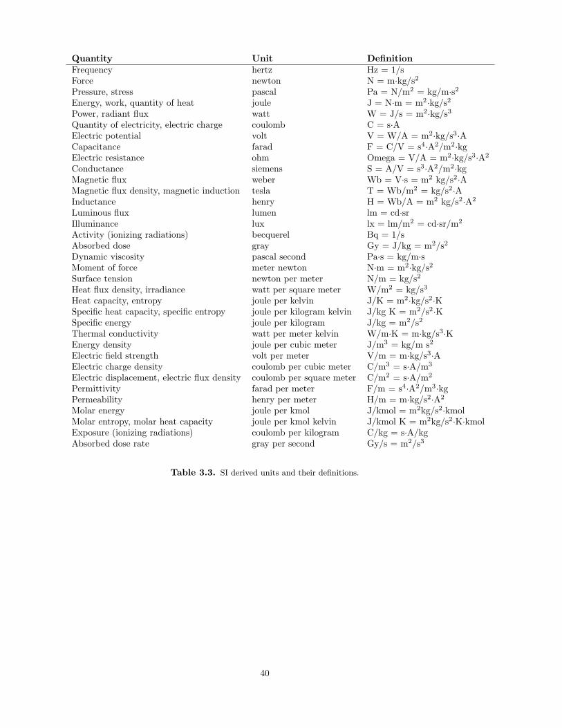
Quantity Unit DefinitionFrequency hertz Hz = 1/sForce newton N = m·kg/s2
Pressure, stress pascal Pa = N/m2 = kg/m·s2Energy, work, quantity of heat joule J = N·m = m2·kg/s2
Power, radiant flux watt W = J/s = m2·kg/s3
Quantity of electricity, electric charge coulomb C = s·AElectric potential volt V = W/A = m2·kg/s3·ACapacitance farad F = C/V = s4·A2/m2·kgElectric resistance ohm Omega = V/A = m2·kg/s3·A2
Conductance siemens S = A/V = s3·A2/m2·kgMagnetic flux weber Wb = V·s = m2 kg/s2·AMagnetic flux density, magnetic induction tesla T = Wb/m2 = kg/s2·AInductance henry H = Wb/A = m2 kg/s2·A2
Luminous flux lumen lm = cd·srIlluminance lux lx = lm/m2 = cd·sr/m2
Activity (ionizing radiations) becquerel Bq = 1/sAbsorbed dose gray Gy = J/kg = m2/s2
Dynamic viscosity pascal second Pa·s = kg/m·sMoment of force meter newton N·m = m2·kg/s2
Surface tension newton per meter N/m = kg/s2
Heat flux density, irradiance watt per square meter W/m2 = kg/s3
Heat capacity, entropy joule per kelvin J/K = m2·kg/s2·KSpecific heat capacity, specific entropy joule per kilogram kelvin J/kg K = m2/s2·KSpecific energy joule per kilogram J/kg = m2/s2
Thermal conductivity watt per meter kelvin W/m·K = m·kg/s3·KEnergy density joule per cubic meter J/m3 = kg/m s2
Electric field strength volt per meter V/m = m·kg/s3·AElectric charge density coulomb per cubic meter C/m3 = s·A/m3
Electric displacement, electric flux density coulomb per square meter C/m2 = s·A/m2
Permittivity farad per meter F/m = s4·A2/m3·kgPermeability henry per meter H/m = m·kg/s2·A2
Molar energy joule per kmol J/kmol = m2kg/s2·kmolMolar entropy, molar heat capacity joule per kmol kelvin J/kmol K = m2kg/s2·K·kmolExposure (ionizing radiations) coulomb per kilogram C/kg = s·A/kgAbsorbed dose rate gray per second Gy/s = m2/s3
Table 3.3. SI derived units and their definitions.
40
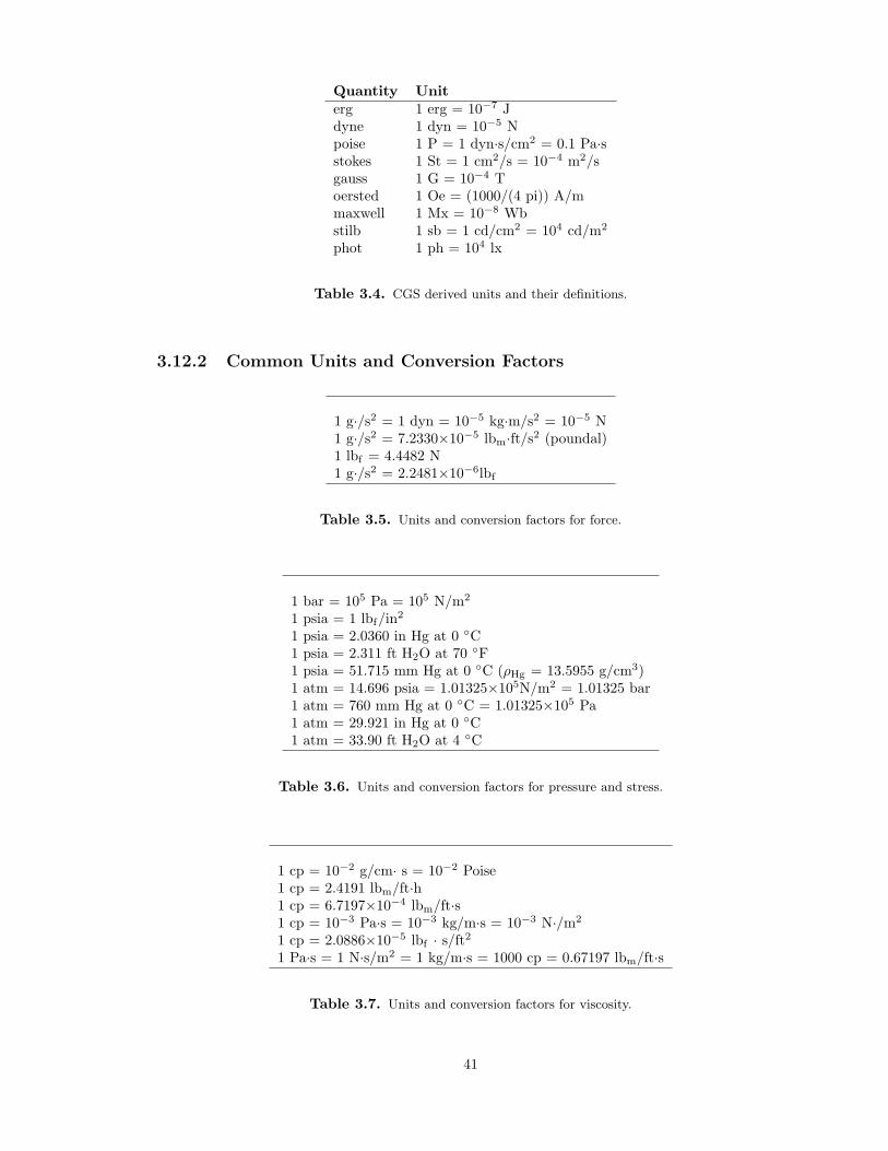
Quantity Uniterg 1 erg = 10−7 Jdyne 1 dyn = 10−5 Npoise 1 P = 1 dyn·s/cm2 = 0.1 Pa·sstokes 1 St = 1 cm2/s = 10−4 m2/sgauss 1 G = 10−4 Toersted 1 Oe = (1000/(4 pi)) A/mmaxwell 1 Mx = 10−8 Wbstilb 1 sb = 1 cd/cm2 = 104 cd/m2
phot 1 ph = 104 lx
Table 3.4. CGS derived units and their definitions.
3.12.2 Common Units and Conversion Factors
1 g·/s2 = 1 dyn = 10−5 kg·m/s2 = 10−5 N1 g·/s2 = 7.2330×10⁻⁵ lbm·ft/s2 (poundal)1 lbf = 4.4482 N1 g·/s2 = 2.2481×10⁻⁶lbf
Table 3.5. Units and conversion factors for force.
1 bar = 105 Pa = 105 N/m2
1 psia = 1 lbf/in2
1 psia = 2.0360 in Hg at 0 C1 psia = 2.311 ft H2O at 70 F1 psia = 51.715 mm Hg at 0 C (ρHg = 13.5955 g/cm3)1 atm = 14.696 psia = 1.01325×10⁵N/m2 = 1.01325 bar1 atm = 760 mm Hg at 0 C = 1.01325×10⁵ Pa1 atm = 29.921 in Hg at 0 C1 atm = 33.90 ft H2O at 4 C
Table 3.6. Units and conversion factors for pressure and stress.
1 cp = 10−2 g/cm· s = 10−2 Poise1 cp = 2.4191 lbm/ft·h1 cp = 6.7197×10⁻⁴ lbm/ft·s1 cp = 10−3 Pa·s = 10−3 kg/m·s = 10−3 N·/m2
1 cp = 2.0886×10⁻⁵ lbf · s/ft2
1 Pa·s = 1 N·s/m2 = 1 kg/m·s = 1000 cp = 0.67197 lbm/ft·s
Table 3.7. Units and conversion factors for viscosity.
41
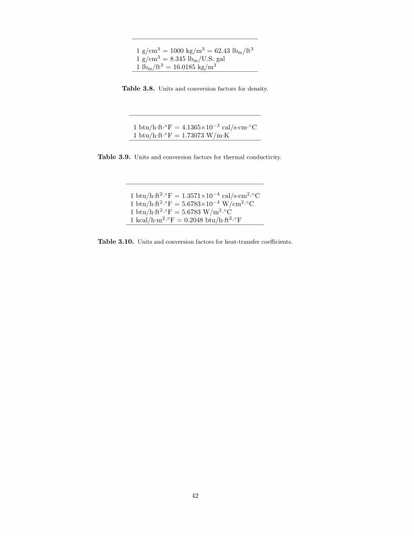
1 g/cm3 = 1000 kg/m3 = 62.43 lbm/ft3
1 g/cm3 = 8.345 lbm/U.S. gal1 lbm/ft3 = 16.0185 kg/m3
Table 3.8. Units and conversion factors for density.
1 btu/h·ft·F = 4.1365×10⁻³ cal/s·cm·C1 btu/h·ft·F = 1.73073 W/m·K
Table 3.9. Units and conversion factors for thermal conductivity.
1 btu/h·ft2·F = 1.3571×10⁻⁴ cal/s·cm2·C1 btu/h·ft2·F = 5.6783×10⁻⁴ W/cm2·C1 btu/h·ft2·F = 5.6783 W/m2·C1 kcal/h·m2·F = 0.2048 btu/h·ft2·F
Table 3.10. Units and conversion factors for heat-transfer coefficients.
42
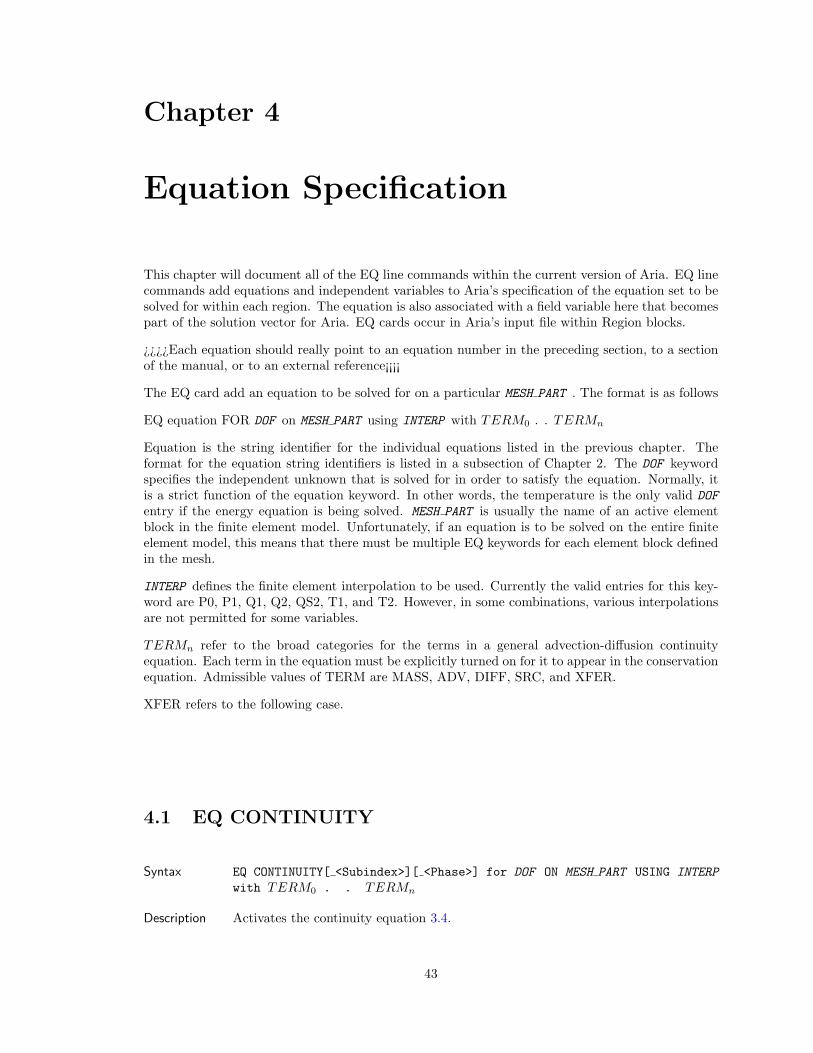
Chapter 4
Equation Specification
This chapter will document all of the EQ line commands within the current version of Aria. EQ linecommands add equations and independent variables to Aria’s specification of the equation set to besolved for within each region. The equation is also associated with a field variable here that becomespart of the solution vector for Aria. EQ cards occur in Aria’s input file within Region blocks.
¿¿¿¿Each equation should really point to an equation number in the preceding section, to a sectionof the manual, or to an external reference¡¡¡¡
The EQ card add an equation to be solved for on a particular MESH PART . The format is as follows
EQ equation FOR DOF on MESH PART using INTERP with TERM0 . . TERMn
Equation is the string identifier for the individual equations listed in the previous chapter. Theformat for the equation string identifiers is listed in a subsection of Chapter 2. The DOF keywordspecifies the independent unknown that is solved for in order to satisfy the equation. Normally, itis a strict function of the equation keyword. In other words, the temperature is the only valid DOF
entry if the energy equation is being solved. MESH PART is usually the name of an active elementblock in the finite element model. Unfortunately, if an equation is to be solved on the entire finiteelement model, this means that there must be multiple EQ keywords for each element block definedin the mesh.
INTERP defines the finite element interpolation to be used. Currently the valid entries for this key-word are P0, P1, Q1, Q2, QS2, T1, and T2. However, in some combinations, various interpolationsare not permitted for some variables.
TERMn refer to the broad categories for the terms in a general advection-diffusion continuityequation. Each term in the equation must be explicitly turned on for it to appear in the conservationequation. Admissible values of TERM are MASS, ADV, DIFF, SRC, and XFER.
XFER refers to the following case.
4.1 EQ CONTINUITY
Syntax EQ CONTINUITY[ <Subindex>][ <Phase>] for DOF ON MESH PART USING INTERP
with TERM0 . . TERMn
Description Activates the continuity equation 3.4.
43
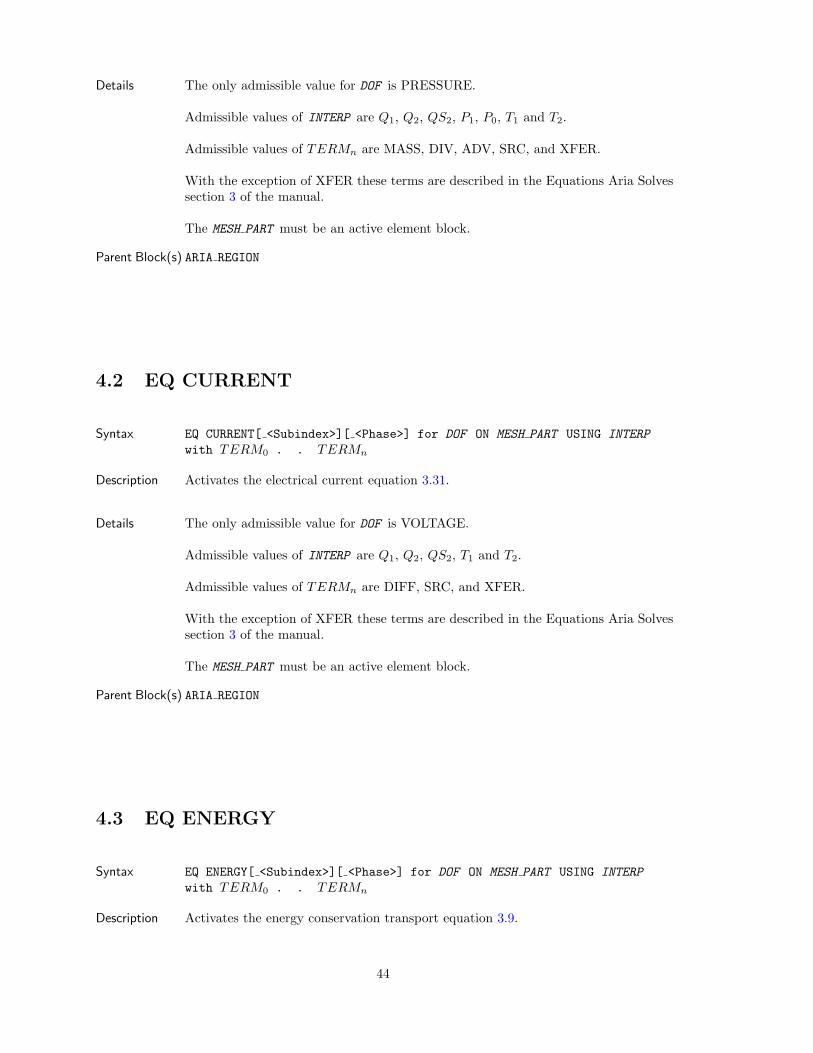
Details The only admissible value for DOF is PRESSURE.
Admissible values of INTERP are Q1, Q2, QS2, P1, P0, T1 and T2.
Admissible values of TERMn are MASS, DIV, ADV, SRC, and XFER.
With the exception of XFER these terms are described in the Equations Aria Solvessection 3 of the manual.
The MESH PART must be an active element block.
Parent Block(s) ARIA REGION
4.2 EQ CURRENT
Syntax EQ CURRENT[ <Subindex>][ <Phase>] for DOF ON MESH PART USING INTERP
with TERM0 . . TERMn
Description Activates the electrical current equation 3.31.
Details The only admissible value for DOF is VOLTAGE.
Admissible values of INTERP are Q1, Q2, QS2, T1 and T2.
Admissible values of TERMn are DIFF, SRC, and XFER.
With the exception of XFER these terms are described in the Equations Aria Solvessection 3 of the manual.
The MESH PART must be an active element block.
Parent Block(s) ARIA REGION
4.3 EQ ENERGY
Syntax EQ ENERGY[ <Subindex>][ <Phase>] for DOF ON MESH PART USING INTERP
with TERM0 . . TERMn
Description Activates the energy conservation transport equation 3.9.
44
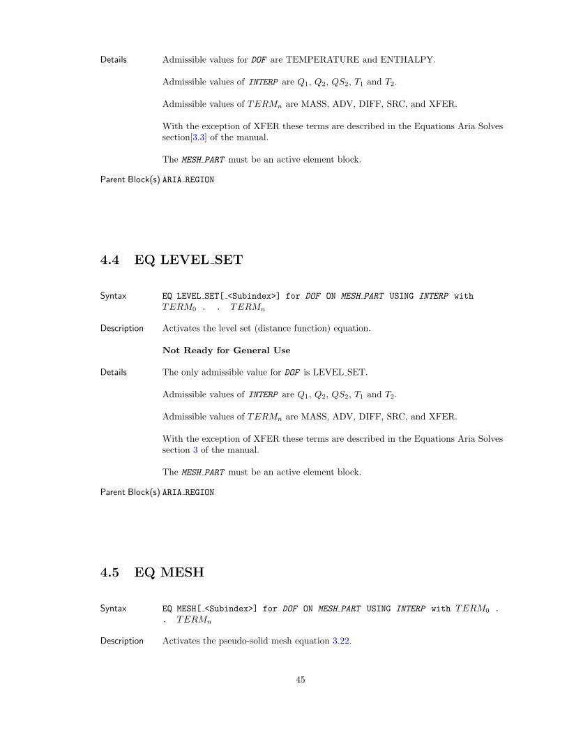
Details Admissible values for DOF are TEMPERATURE and ENTHALPY.
Admissible values of INTERP are Q1, Q2, QS2, T1 and T2.
Admissible values of TERMn are MASS, ADV, DIFF, SRC, and XFER.
With the exception of XFER these terms are described in the Equations Aria Solvessection[3.3] of the manual.
The MESH PART must be an active element block.
Parent Block(s) ARIA REGION
4.4 EQ LEVEL SET
Syntax EQ LEVEL SET[ <Subindex>] for DOF ON MESH PART USING INTERP withTERM0 . . TERMn
Description Activates the level set (distance function) equation.
Not Ready for General Use
Details The only admissible value for DOF is LEVEL SET.
Admissible values of INTERP are Q1, Q2, QS2, T1 and T2.
Admissible values of TERMn are MASS, ADV, DIFF, SRC, and XFER.
With the exception of XFER these terms are described in the Equations Aria Solvessection 3 of the manual.
The MESH PART must be an active element block.
Parent Block(s) ARIA REGION
4.5 EQ MESH
Syntax EQ MESH[ <Subindex>] for DOF ON MESH PART USING INTERP with TERM0 .. TERMn
Description Activates the pseudo-solid mesh equation 3.22.
45
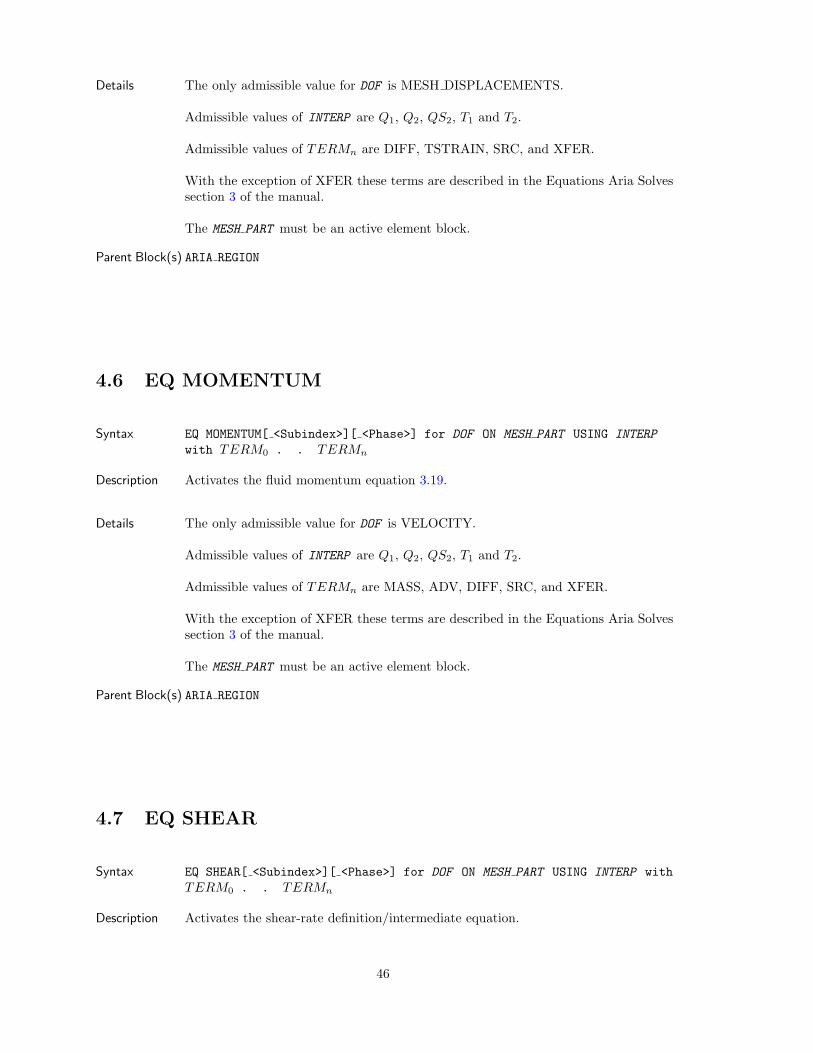
Details The only admissible value for DOF is MESH DISPLACEMENTS.
Admissible values of INTERP are Q1, Q2, QS2, T1 and T2.
Admissible values of TERMn are DIFF, TSTRAIN, SRC, and XFER.
With the exception of XFER these terms are described in the Equations Aria Solvessection 3 of the manual.
The MESH PART must be an active element block.
Parent Block(s) ARIA REGION
4.6 EQ MOMENTUM
Syntax EQ MOMENTUM[ <Subindex>][ <Phase>] for DOF ON MESH PART USING INTERP
with TERM0 . . TERMn
Description Activates the fluid momentum equation 3.19.
Details The only admissible value for DOF is VELOCITY.
Admissible values of INTERP are Q1, Q2, QS2, T1 and T2.
Admissible values of TERMn are MASS, ADV, DIFF, SRC, and XFER.
With the exception of XFER these terms are described in the Equations Aria Solvessection 3 of the manual.
The MESH PART must be an active element block.
Parent Block(s) ARIA REGION
4.7 EQ SHEAR
Syntax EQ SHEAR[ <Subindex>][ <Phase>] for DOF ON MESH PART USING INTERP withTERM0 . . TERMn
Description Activates the shear-rate definition/intermediate equation.
46
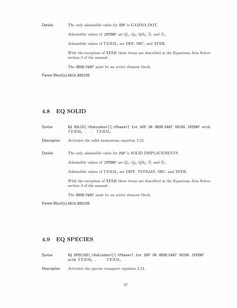
Details The only admissible value for DOF is GAMMA DOT.
Admissible values of INTERP are Q1, Q2, QS2, T1 and T2.
Admissible values of TERMn are DEF, SRC, and XFER.
With the exception of XFER these terms are described in the Equations Aria Solvessection 3 of the manual.
The MESH PART must be an active element block.
Parent Block(s) ARIA REGION
4.8 EQ SOLID
Syntax EQ SOLID[ <Subindex>][ <Phase>] for DOF ON MESH PART USING INTERP withTERM0 . . TERMn
Description Activates the solid momentum equation 3.22.
Details The only admissible value for DOF is SOLID DISPLACEMENTS.
Admissible values of INTERP are Q1, Q2, QS2, T1 and T2.
Admissible values of TERMn are DIFF, TSTRAIN, SRC, and XFER.
With the exception of XFER these terms are described in the Equations Aria Solvessection 3 of the manual.
The MESH PART must be an active element block.
Parent Block(s) ARIA REGION
4.9 EQ SPECIES
Syntax EQ SPECIES[ <Subindex>][ <Phase>] for DOF ON MESH PART USING INTERP
with TERM0 . . TERMn
Description Activates the species transport equation 3.13.
47
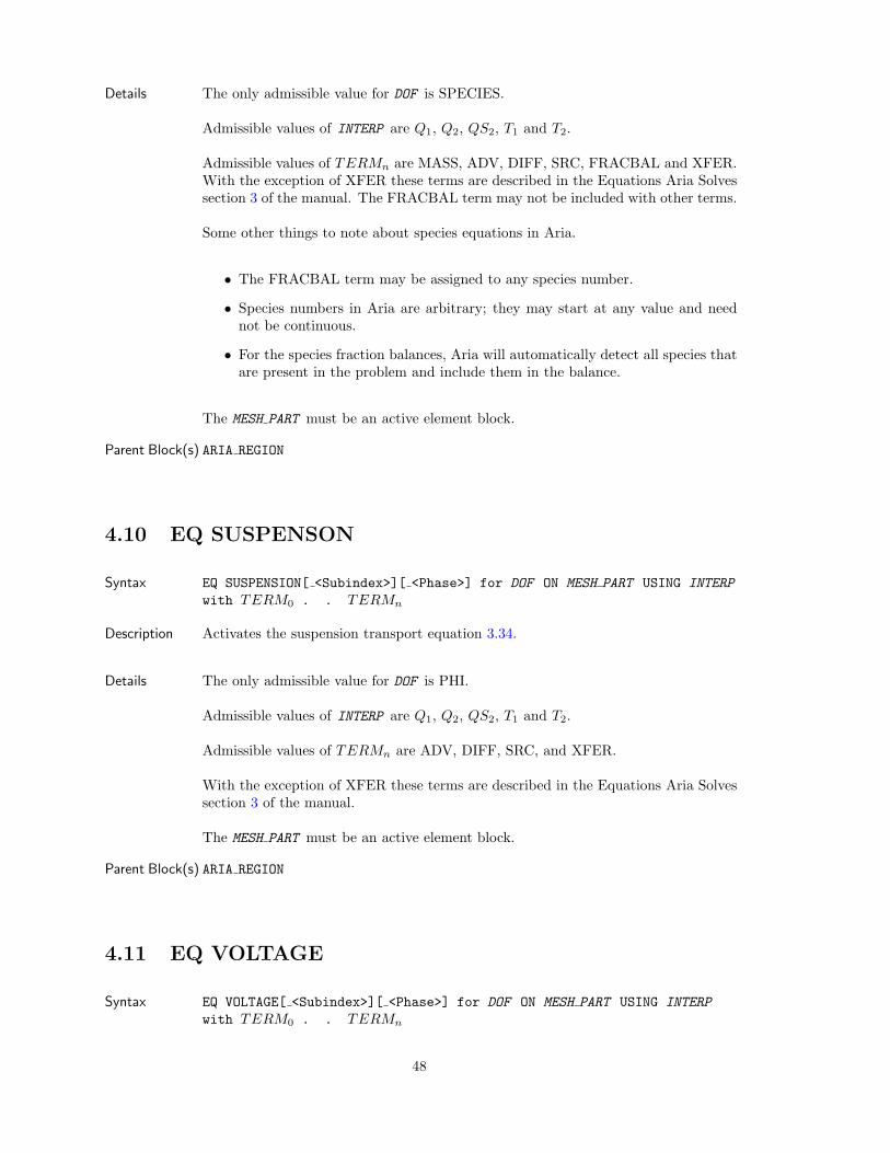
Details The only admissible value for DOF is SPECIES.
Admissible values of INTERP are Q1, Q2, QS2, T1 and T2.
Admissible values of TERMn are MASS, ADV, DIFF, SRC, FRACBAL and XFER.With the exception of XFER these terms are described in the Equations Aria Solvessection 3 of the manual. The FRACBAL term may not be included with other terms.
Some other things to note about species equations in Aria.
• The FRACBAL term may be assigned to any species number.
• Species numbers in Aria are arbitrary; they may start at any value and neednot be continuous.
• For the species fraction balances, Aria will automatically detect all species thatare present in the problem and include them in the balance.
The MESH PART must be an active element block.
Parent Block(s) ARIA REGION
4.10 EQ SUSPENSON
Syntax EQ SUSPENSION[ <Subindex>][ <Phase>] for DOF ON MESH PART USING INTERP
with TERM0 . . TERMn
Description Activates the suspension transport equation 3.34.
Details The only admissible value for DOF is PHI.
Admissible values of INTERP are Q1, Q2, QS2, T1 and T2.
Admissible values of TERMn are ADV, DIFF, SRC, and XFER.
With the exception of XFER these terms are described in the Equations Aria Solvessection 3 of the manual.
The MESH PART must be an active element block.
Parent Block(s) ARIA REGION
4.11 EQ VOLTAGE
Syntax EQ VOLTAGE[ <Subindex>][ <Phase>] for DOF ON MESH PART USING INTERP
with TERM0 . . TERMn
48
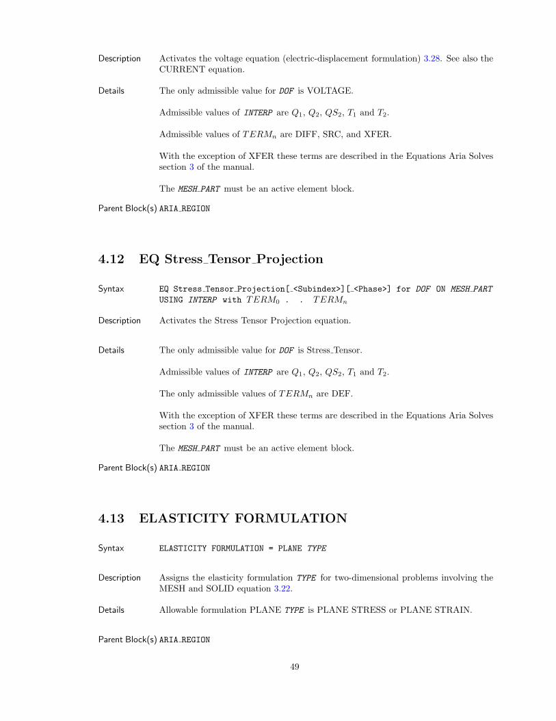
Description Activates the voltage equation (electric-displacement formulation) 3.28. See also theCURRENT equation.
Details The only admissible value for DOF is VOLTAGE.
Admissible values of INTERP are Q1, Q2, QS2, T1 and T2.
Admissible values of TERMn are DIFF, SRC, and XFER.
With the exception of XFER these terms are described in the Equations Aria Solvessection 3 of the manual.
The MESH PART must be an active element block.
Parent Block(s) ARIA REGION
4.12 EQ Stress Tensor Projection
Syntax EQ Stress Tensor Projection[ <Subindex>][ <Phase>] for DOF ON MESH PART
USING INTERP with TERM0 . . TERMn
Description Activates the Stress Tensor Projection equation.
Details The only admissible value for DOF is Stress Tensor.
Admissible values of INTERP are Q1, Q2, QS2, T1 and T2.
The only admissible values of TERMn are DEF.
With the exception of XFER these terms are described in the Equations Aria Solvessection 3 of the manual.
The MESH PART must be an active element block.
Parent Block(s) ARIA REGION
4.13 ELASTICITY FORMULATION
Syntax ELASTICITY FORMULATION = PLANE TYPE
Description Assigns the elasticity formulation TYPE for two-dimensional problems involving theMESH and SOLID equation 3.22.
Details Allowable formulation PLANE TYPE is PLANE STRESS or PLANE STRAIN.
Parent Block(s) ARIA REGION
49
4.14 PRESSURE STABILIZATION
Syntax PRESSURE STABILIZATION IS TYPE WITH SCALING = C
Description Prescribe a stabilization technique for solving the MOMENTUM 3.19 and CONTINUITY 3.4equations with equal order interpolation.
Details Aria supports both PSPG (Pressure Stabilizide Petrov-Gelerkin) and PSPP (PressureStabilized Pressure Projection) stabilization techniques for solving the MOMENTUM andCONTINUITY equations with equal order interpolation.
Valid options for the TYPE specification are NO STABILIZATION, PSPG CONSTANT,PSPG LOCAL, PSPG GLOBAL and PSPP CONSTANT.
NO STABILIZATION disables any stabilization.
PSPP CONSTANT results in the recently developed stabilization technique of Dohrmannand Bochev (2004) and Bochev et al. (2006).
In the PSPG forms of stabilization, introduced by Hughes et al. (1986), terms fromthe momentum equation are added to the continuity equation scaled by a multiplier,α. The exact form of the multipler depend on a global Reynolds number that isdefined as
Re ≡ ρ|v|〈h〉2µ
(4.1)
Here, ρ is the density, µ is the viscosity, |v| is a velocity scale and 〈h〉 is an elementlength scale. Armed with Re, the stabilization multipler α is defined in one of twoways.
Re ≤ 3 : α ≡ τ〈h〉2
12µ(4.2)
Re > 3 : α ≡ τ〈h〉2ρ|v|
(4.3)
NB: Currently, Aria always uses the low-Reynolds number for of α, as defined in(4.2). The PSPG LOCAL method computes |v| and 〈h〉 within each element. ThePSPG GLOBAL method computes |v| and 〈h〉 as averages over all of the elements withthe MOMENTUM equation defined. The PSPG CONSTANT gives |v| and 〈h〉 a value of 1(one) and just uses the scale factor.
Parent Block(s) ARIA REGION
4.15 MESH MOTION
Syntax MESH MOTION IS TYPE ON MESH PART
50
Description Defines the type of mesh motion to be used in the simulation.
Details Admissible values of TYPE are ARBITRARY, LAGRANGIAN, and TOTAL ALE.When TYPE is ARBITRARY or TOTAL ALE the MESH equation must be active.When TYPE is LAGRANGIAN or TOTAL ALE the SOLID equation must be active.The MESH PART must be an active element block.
Parent Block(s) ARIA REGION
4.16 SAVE RESIDUALS
Syntax SAVE RESIDUALS = MODE
Description Causes Aria to save the residuals to a field with the prefix residaul->, e.g.,residual->Temperature. This will be done for all fields (though we could makeit a per-field option). Valid choices are OFF (default), BEFORE BCS and AFTER BCS.
Details Causes Aria to save the residuals to a field with the prefix residaul->, e.g.,residual->Temperature. This will be done for all fields (though we could makeit a per-field option). Valid choices are OFF (default), BEFORE BCS and AFTER BCS.
For the choice BEFORE BCS the residuals will be saved at the point in the assemblyprocess where the primary equations have been assembled but prior to the assemblyof any boundary conditions or distinguishing conditions. For the choice of AFTER BCSthe residuals will be saved after all BCs and distinguishing conditions have beenapplied. The default, OFF, is to not save the residuals.
This feature is only applicable when using the NEWTON nonlinear solution strategy.
Parent Block(s) ARIA REGION
4.17 INTEGRATION RULE
Syntax INTEGRATION RUL for block name = INT
Description Overrides the default integration rule for the equations defined on block name .
Details Overrides the default integration rule for the equations defined on block name .
Parent Block(s) ARIA REGION
51

52
Chapter 5
Initial Conditions
5.1 IC CIRC X
Syntax IC CIRC X AT MESH PART DOF AMP = Ω
Description Initial boundary condition for the x component of a vector variable with constanttangential magnitude along circles of radius r(x, y) defined on the mesh entity.
Details Sets DOF to the provided value on nodeset associated with the nameMESH PART according to the relation
DOF = −Ωr(x, y) sin θ. (5.1)
The rotation Ω is assumed to be about the vector (0, 0, 1) passing through point(0, 0, 0).
Parent Block(s) ARIA REGION
5.2 IC CIRC Y
Syntax IC CIRC Y AT MESH PART DOF AMP = Ω
Description Initial boundary condition for the y component of a vector variable with constanttangential magnitude along circles of radius r(x, y) defined on the mesh entity.
Details Sets DOF to the provided value on nodeset associated with the nameMESH PART according to the relation
DOF = Ωr(x, y) cos θ. (5.2)
The rotation Ω is assumed to be about the vector (0, 0, 1) passing through point(0, 0, 0).
Parent Block(s) ARIA REGION
53
5.3 IC CONSTANT
Syntax IC CONST AT MESH PART DOF = REAL
Description Constant initial condition.
Details Sets DOF to the provided constant value on mesh entity associated with the nameMESH PART .
Parent Block(s) ARIA REGION
5.4 IC COUETTE X
Syntax IC COUETTE X AT MESH PART DOF PARAMS = Ω ri ro
Description Initial condition for x component of a vector variable in a Couette device with innerradius ri, outer radius ro and driven at angular velocity Ω, that varies spatially overa mesh entity.
Details Sets DOF to vary spatially over the nodeset associated with the nameMESH PART according to the relation
DOF = −Ωr(x, y)riro
r2o − r2
i
sin θ. (5.3)
The rotation Ω is assumed to be about the vector (0, 0, 1) passing through point(0, 0, 0).
Parent Block(s) ARIA REGION
5.5 IC COUETTE Y
Syntax IC COUETTE Y AT MESH PART DOF PARAMS = Ω ri ro
Description Initial condition for x component of a vector variable in a Couette device with innerradius ri, outer radius ro and driven at angular velocity Ω, that varies spatially overa mesh entity.
Details Sets DOF to vary spatially over the nodeset associated with the nameMESH PART according to the relation
DOF = Ωr(x, y)riro
r2o − r2
i
cos θ. (5.4)
The rotation Ω is assumed to be about the vector (0, 0, 1) passing through point(0, 0, 0).
54
Parent Block(s) ARIA REGION
5.6 IC COUETTE SH
Syntax IC COUETTE SH AT MESH PART DOF PARAMS = Ω ri ro
Description Initial condition for generalized shear rate in a Couette device with inner radius ri,outer radius ro and driven at angular velocity Ω, that varies spatially over a meshentity.
Details Sets DOF to the provided value on nodeset associated with the nameMESH PART according to the relation
DOF =Ω
r2(x, y)riro
r2o − r2
i
(1
r(x, y)− r(x, y)
r2o
)(5.5)
The rotation Ω is assumed to be about the vector (0, 0, 1) passing through point(0, 0, 0).
Parent Block(s) ARIA REGION
5.7 IC READ FILE
Syntax IC Read File DOF = STRING
Description This IC command will initialize the field DOF with values from the field with thename given by the STRING argument in the input mesh database.
Details This IC command will initialize the field DOF with values from the field with the namegiven by the STRING argument in the input mesh database. For example, if your inputmesh database (the file referenced in the FINITE ELEMENT MODEL) contains a vectorfield named U then you could initialize a velocity field by setting DOF to VELOCITYand the STRING argument to U.
Parent Block(s) ARIA REGION
5.8 IC LINEAR
Syntax IC LINEAR AT MESH PART DOF COEF = C0 C1 C2 C3
Description Initial condition that varies spatially over a mesh entity in a linear fashion.
55
Details Sets DOF to the provided value on nodeset associated with the name MESH PART inthe following manner
DOF = C0 + C1x + C2y + C3z. (5.6)
Parent Block(s) ARIA REGION
5.9 IC PARAB
Syntax IC PARAB AT MESH PART DOF COEF = C0 C1 C2 C3 C4 C5 C6 C7 C8 C9
Description Initial condition that varies spatially over a mesh entity in a parabolic fashion.
Details Sets DOF to the provided value on nodeset associated with the name MESH PART inthe following manner
DOF = C0 + C1x + C2y + C3z + C4xy + C5xz + C6yz + C7x2 + C8y
2 + C9z2. (5.7)
Parent Block(s) ARIA REGION
56
Chapter 6
Boundary Conditions
This chapter documents the boundary condition, BC, line commands within the current version ofAria. In what follows, Dirichlet boundary conditions are first described and are followed by fluxboundary condition descriptions.
6.1 BC CIRC X
Syntax BC CIRC X DIRICHLET AT MESH PART DOF AMP = Ω
Description Dirichlet boundary condition for the x component of a vector variable with constanttangential magnitude along circles of radius r(x, y) defined on the mesh entity.
Details Sets DOF to the provided value on nodeset associated with the nameMESH PART according to the relation
DOF = −Ωr(x, y) sin θ. (6.1)
The rotation Ω is assumed to be about the vector (0, 0, 1) passing through point(0, 0, 0).
Parent Block(s) ARIA REGION
6.2 BC CIRC Y
Syntax BC CIRC Y DIRICHLET AT MESH PART DOF AMP = Ω
Description Dirichlet boundary condition for the y component of a vector variable with constanttangential magnitude along circles of radius r(x, y) defined on the mesh entity.
Details Sets DOF to the provided value on nodeset associated with the nameMESH PART according to the relation
DOF = Ωr(x, y) cos θ. (6.2)
The rotation Ω is assumed to be about the vector (0, 0, 1) passing through point(0, 0, 0).
57
Parent Block(s) ARIA REGION
6.3 BC CONST
Syntax BC CONST DIRICHLET AT MESH PART DOF = REAL
Description Constant Dirichlet condition.
Details Sets DOF to the provided constant value on mesh entity associated with the nameMESH PART .
Parent Block(s) ARIA REGION
6.4 BC LINEAR
Syntax BC LINEAR DIRICHLET AT MESH PART DOF COEF = C0 C1 C2 C3
Description Dirichlet boundary condition that varies spatially over a mesh entity in a linearfashion.
Details Sets DOF to the provided value on nodeset associated with the name MESH PART inthe following manner
DOF = C0 + C1x + C2y + C3z. (6.3)
Parent Block(s) ARIA REGION
6.5 BC LINEAR IN TIME
Syntax BC LINEAR IN TIME DIRICHLET AT MESH PART DOF = C0 C1
Description Dirichlet boundary condition whose value is a linear function in time.
Details Sets DOF to the provided value on nodeset associated with the nameMESH PART according to the relation
DOF = C0 + C1t (6.4)
Parent Block(s) ARIA REGION
58
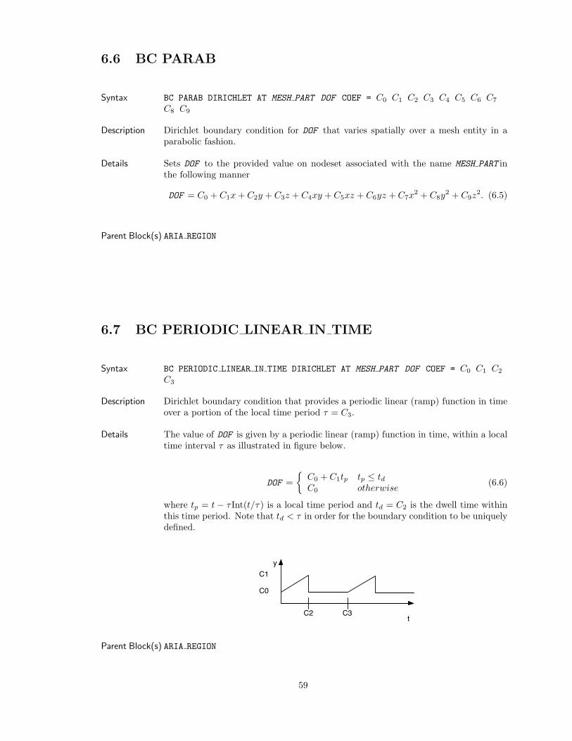
6.6 BC PARAB
Syntax BC PARAB DIRICHLET AT MESH PART DOF COEF = C0 C1 C2 C3 C4 C5 C6 C7
C8 C9
Description Dirichlet boundary condition for DOF that varies spatially over a mesh entity in aparabolic fashion.
Details Sets DOF to the provided value on nodeset associated with the name MESH PART inthe following manner
DOF = C0 + C1x + C2y + C3z + C4xy + C5xz + C6yz + C7x2 + C8y
2 + C9z2. (6.5)
Parent Block(s) ARIA REGION
6.7 BC PERIODIC LINEAR IN TIME
Syntax BC PERIODIC LINEAR IN TIME DIRICHLET AT MESH PART DOF COEF = C0 C1 C2
C3
Description Dirichlet boundary condition that provides a periodic linear (ramp) function in timeover a portion of the local time period τ = C3.
Details The value of DOF is given by a periodic linear (ramp) function in time, within a localtime interval τ as illustrated in figure below.
DOF =
C0 + C1tp tp ≤ tdC0 otherwise
(6.6)
where tp = t − τ Int(t/τ) is a local time period and td = C2 is the dwell time withinthis time period. Note that td < τ in order for the boundary condition to be uniquelydefined.
t
C0
C1
C2 C3
y
Parent Block(s) ARIA REGION
59
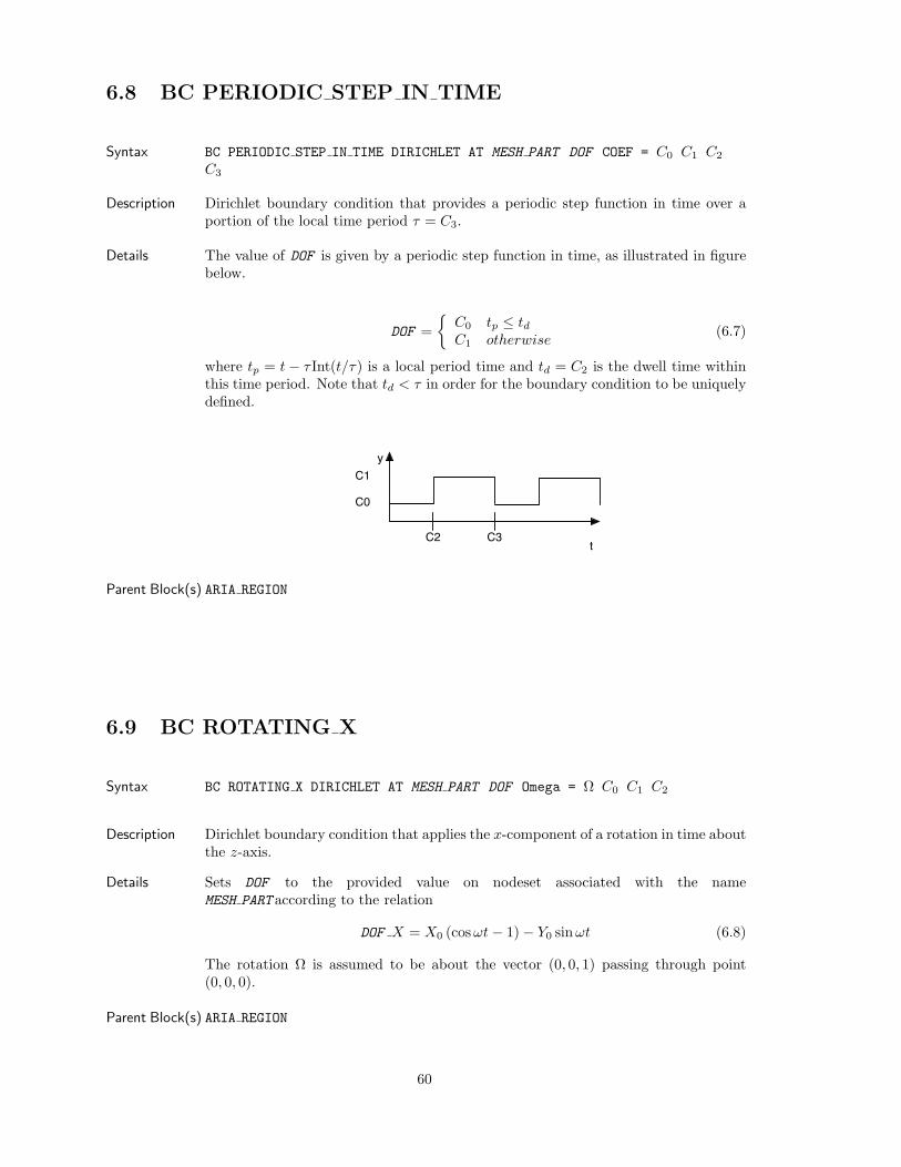
6.8 BC PERIODIC STEP IN TIME
Syntax BC PERIODIC STEP IN TIME DIRICHLET AT MESH PART DOF COEF = C0 C1 C2
C3
Description Dirichlet boundary condition that provides a periodic step function in time over aportion of the local time period τ = C3.
Details The value of DOF is given by a periodic step function in time, as illustrated in figurebelow.
DOF =
C0 tp ≤ tdC1 otherwise
(6.7)
where tp = t − τ Int(t/τ) is a local period time and td = C2 is the dwell time withinthis time period. Note that td < τ in order for the boundary condition to be uniquelydefined.
t
C0
C1
C2 C3
y
Parent Block(s) ARIA REGION
6.9 BC ROTATING X
Syntax BC ROTATING X DIRICHLET AT MESH PART DOF Omega = Ω C0 C1 C2
Description Dirichlet boundary condition that applies the x-component of a rotation in time aboutthe z-axis.
Details Sets DOF to the provided value on nodeset associated with the nameMESH PART according to the relation
DOF X = X0 (cos ωt− 1)− Y0 sinωt (6.8)
The rotation Ω is assumed to be about the vector (0, 0, 1) passing through point(0, 0, 0).
Parent Block(s) ARIA REGION
60
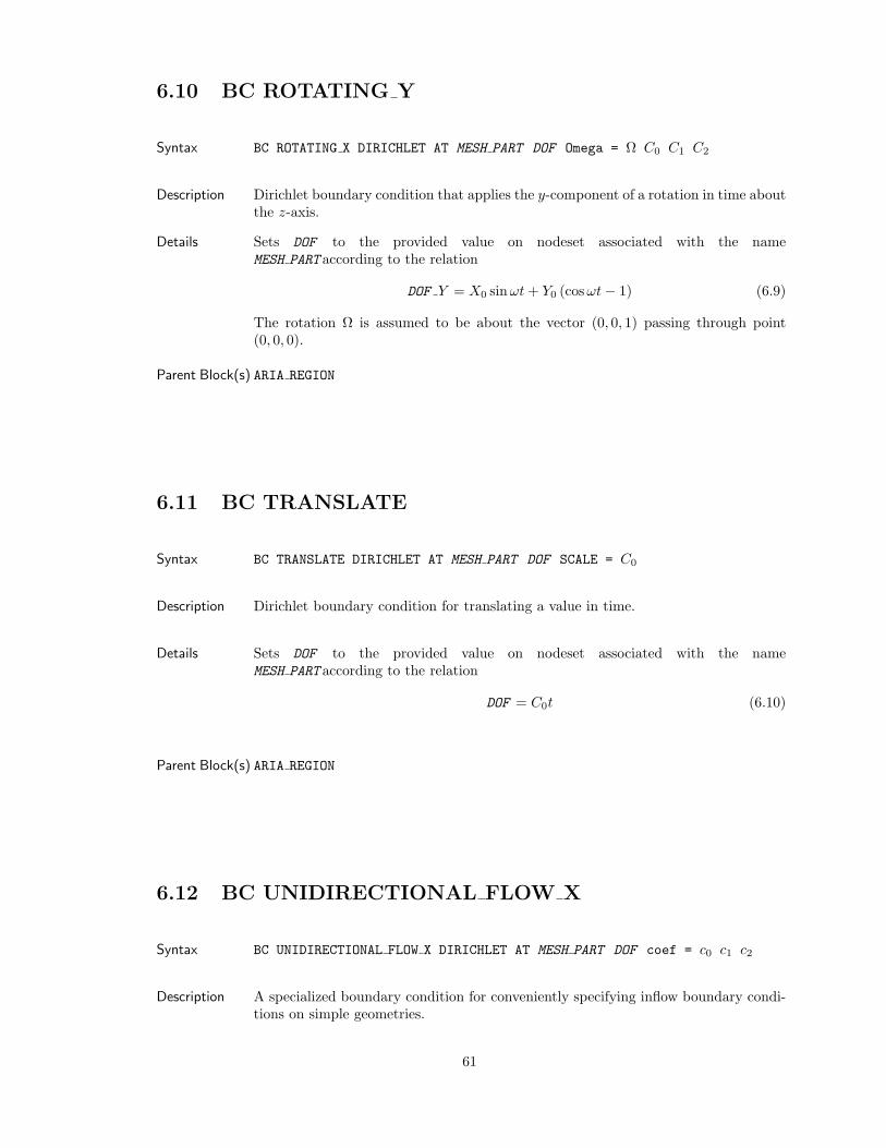
6.10 BC ROTATING Y
Syntax BC ROTATING X DIRICHLET AT MESH PART DOF Omega = Ω C0 C1 C2
Description Dirichlet boundary condition that applies the y-component of a rotation in time aboutthe z-axis.
Details Sets DOF to the provided value on nodeset associated with the nameMESH PART according to the relation
DOF Y = X0 sinωt + Y0 (cos ωt− 1) (6.9)
The rotation Ω is assumed to be about the vector (0, 0, 1) passing through point(0, 0, 0).
Parent Block(s) ARIA REGION
6.11 BC TRANSLATE
Syntax BC TRANSLATE DIRICHLET AT MESH PART DOF SCALE = C0
Description Dirichlet boundary condition for translating a value in time.
Details Sets DOF to the provided value on nodeset associated with the nameMESH PART according to the relation
DOF = C0t (6.10)
Parent Block(s) ARIA REGION
6.12 BC UNIDIRECTIONAL FLOW X
Syntax BC UNIDIRECTIONAL FLOW X DIRICHLET AT MESH PART DOF coef = c0 c1 c2
Description A specialized boundary condition for conveniently specifying inflow boundary condi-tions on simple geometries.
61
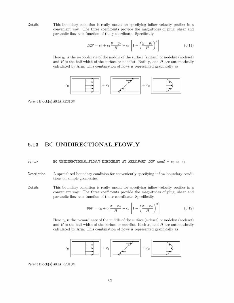
Details This boundary condition is really meant for specifying inflow velocity profiles in aconvenient way. The three coefficients provide the magnitudes of plug, shear andparabolic flow as a function of the y-coordinate. Specifically,
DOF = c0 + c1y − y
H+ c2
[1−
(y − y
H
)2]
(6.11)
Here y is the y-coordinate of the middle of the surface (sideset) or nodelist (nodeset)and H is the half-width of the surface or nodelist. Both y and H are automaticallycalculated by Aria. This combination of flows is represented graphically as
c0 + c1 + c2
Parent Block(s) ARIA REGION
6.13 BC UNIDIRECTIONAL FLOW Y
Syntax BC UNIDIRECTIONAL FLOW Y DIRICHLET AT MESH PART DOF coef = c0 c1 c2
Description A specialized boundary condition for conveniently specifying inflow boundary condi-tions on simple geometries.
Details This boundary condition is really meant for specifying inflow velocity profiles in aconvenient way. The three coefficients provide the magnitudes of plug, shear andparabolic flow as a function of the x-coordinate. Specifically,
DOF = c0 + c1x− x
H+ c2
[1−
(x− x
H
)2]
(6.12)
Here x is the x-coordinate of the middle of the surface (sideset) or nodelist (nodeset)and H is the half-width of the surface or nodelist. Both x and H are automaticallycalculated by Aria. This combination of flows is represented graphically as
c0 + c1 + c2
Parent Block(s) ARIA REGION
62
6.14 BC FLUX
Syntax BC FLUX FOR EQNAME ON MESH PART = MODEL [param1 = val1, param2 = val2
...]
Description Neumann boundary condition that sets the surface normal flux of the degree of free-dom associated with equation EQNAME to that provided by the specified MODEL .
Details MODEL the supplies a diffusive flux fn ≡ n · f in accordance with equation 3.3. I.e.,it adds the surface integral ∫
MESH PART
n · fφi dS (6.13)
to the residual for equation EQNAME . See, e.g., qn in equation 3.10.
Parent Block(s) ARIA REGION
6.14.1 BC FLUX = CONSTANT
Parameters FLUX = REAL
Example BC Flux for Energy on surface 10 = Constant Flux=3.14159
Description FLUX is the value of the constant flux where positive values indicate a loss, i.e., positiveflux leavse the volume.
6.14.2 BC FLUX = ENCLOSURE RADIATION
Parameters [MULTIPLIER = REAL ]
Example BC Flux for Energy on surface 10 = Enclosure Radiation
Description This boundary condition incorporates the heat flux that’s computed using Chaparralfor enclosure radiation.
See chapter 21 for more information on enclosure radiation.
6.14.3 BC FLUX = LASER
Parameters TON = REAL
TOFF = REAL
X0 = REAL
Y0 = REAL
R0 = REAL W = REAL
FLUX = REAL
RLASER = REAL
63
Example BC Flux for Energy on surface 10 = Laser ton=0 toff=10 x0=0 y0=0 w=1.0rlaser=0.025 flux=3.14159 r0=0.01
Description This boundary condition imposes an energy flux due to an incident laser. The laseris directed in the z direction and travels in a circular path.
TON is the time when the laser is turned on.
TOFF is the time when the laser is turned off.
X0 is the x coordinate of the center of the laser path.
Y0 is the y coordinate of the center of the laser path.
W is the angular velocity of the laser.
FLUX is the value of the energy flux into the surface. (The usual convention is thatpositive fluxes indicate loss.)
RLASER is the radius of the laser beam.
6.14.4 BC FLUX = LASER WELD
Parameters PATH FUNCTION = STRING
FLUX = REAL
RLASER = REAL
[NORMAL TOLERANCE = REAL ]
Example # This function lives at the top level, inside the ’Begin Sierra’block
Begin Definition for Function PATHType is Multicolumn Piecewise LinearColumn Titles Time X Y ZBegin Values0.0000000E+00 0.0000000E+00 0.0000000E+00 0.0000000E+000.2250000E+00 0.1500000E+00 0.0000000E+00 0.0000000E+000.2328540E+00 0.1552336E+00 -0.1370490E-03 0.0000000E+00...
EndEnd
# This goes in the Aria Region with all of the other BCsBC Flux for Energy on surface 10 = Laser Path Function=PATHRlaser=0.025 Flux=3.14159
64
Description This boundary condition imposes an energy flux due to an incident laser. The po-sition of the laser is dictated by a user supplied function which contains x, y and zcoordinates as a function of time; Aria uses linear piecewise interpolation to obtainthe location of the laser at a given time.
PATH is the name of the user supplied function which has time as the first columnand contains columns titled X, Y and Z containing the x, y and z coordinates.
FLUX is the value of the energy flux into the surface. (The usual convention is thatpositive fluxes indicate loss.)
RLASER is the radius of the laser beam.
The determination of whether a point in space has an incident laser flux is done asfollows. At time t the laser is at a point P and the Laser Weld boundary condition isbeing evaluated at a point x (typically an integration point). The distance of x fromP is defined as r ≡ P −x. If a tolerance NORMAL TOLERANCE is supplied and the out-of-surface portion of r is greater than the tolerance then the flux is taken to be zero.Otherwise, the out-of-surface portion of r is subtracted to neglect minor differencesbetween the PATH FUNCTION and the discretized mesh, rs ≡ r − (n · r)n where n isthe outward unit normal at x. If |rs| < RLASER then the point x is considered to bein the beam and the flux is applied; otherwise, no flux is applied.
6.14.5 BC FLUX = SPOT WELD
Parameters SRC X = REAL
SRC Y = REAL
[SRC Z = REAL ]DIR X = REAL
DIR Y = REAL
[DIR Z = REAL ]FLUX = REAL
R = REAL
[TON = REAL ][TOFF = REAL ]
Example BC Flux for Energy on surface 10 = Spot Weld Src X=0 Src Y=3 Dir X=0Dir Y=-1 Flux=1000 R=0.01
65
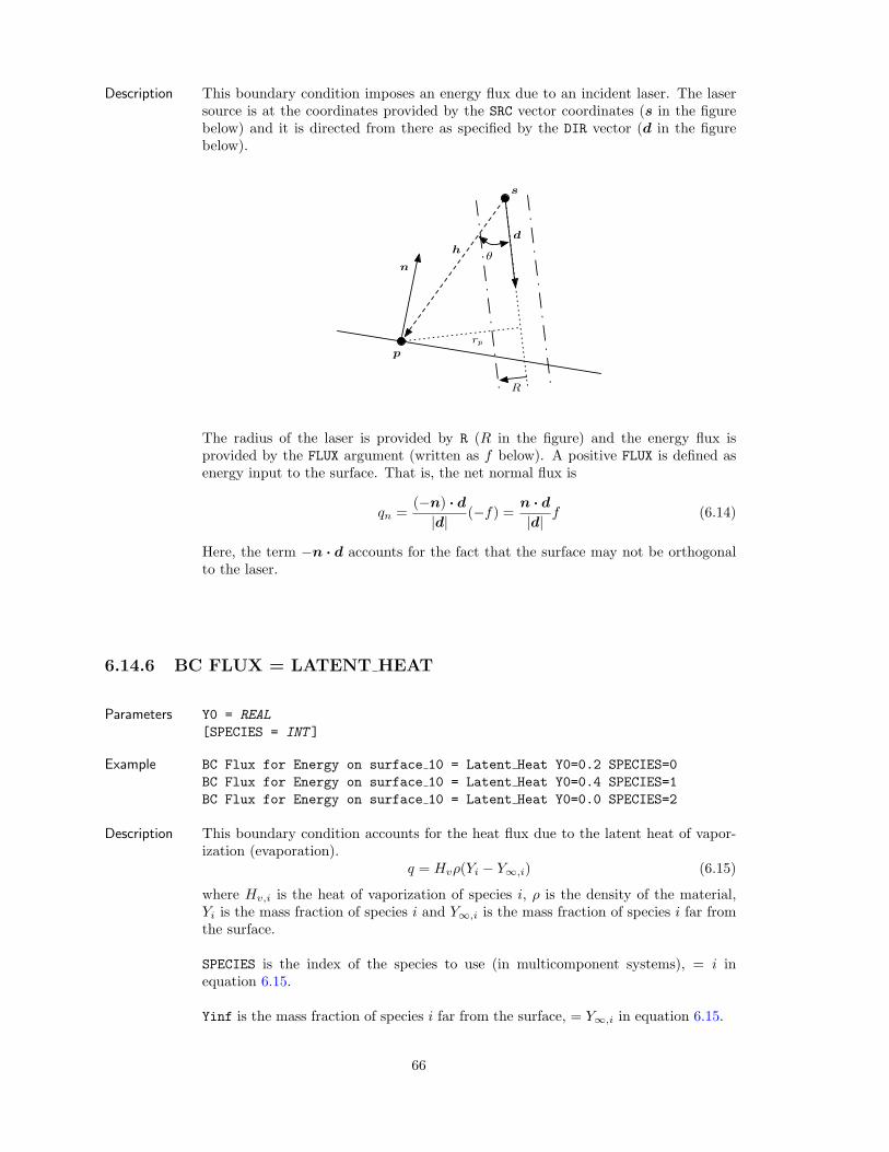
Description This boundary condition imposes an energy flux due to an incident laser. The lasersource is at the coordinates provided by the SRC vector coordinates (s in the figurebelow) and it is directed from there as specified by the DIR vector (d in the figurebelow).
!h
d
s
p
n
rp
R
The radius of the laser is provided by R (R in the figure) and the energy flux isprovided by the FLUX argument (written as f below). A positive FLUX is defined asenergy input to the surface. That is, the net normal flux is
qn =(−n) · d
|d|(−f) =
n · d
|d|f (6.14)
Here, the term −n · d accounts for the fact that the surface may not be orthogonalto the laser.
6.14.6 BC FLUX = LATENT HEAT
Parameters Y0 = REAL
[SPECIES = INT ]
Example BC Flux for Energy on surface 10 = Latent Heat Y0=0.2 SPECIES=0BC Flux for Energy on surface 10 = Latent Heat Y0=0.4 SPECIES=1BC Flux for Energy on surface 10 = Latent Heat Y0=0.0 SPECIES=2
Description This boundary condition accounts for the heat flux due to the latent heat of vapor-ization (evaporation).
q = Hvρ(Yi − Y∞,i) (6.15)
where Hv,i is the heat of vaporization of species i, ρ is the density of the material,Yi is the mass fraction of species i and Y∞,i is the mass fraction of species i far fromthe surface.
SPECIES is the index of the species to use (in multicomponent systems), = i inequation 6.15.
Yinf is the mass fraction of species i far from the surface, = Y∞,i in equation 6.15.
66
6.14.7 BC FLUX = NAT CONV
Parameters T0 = REAL
H = REAL
Example BC Flux for Energy on surface 10 = Nat Conv T0=273.15 H=300
Description This boundary condition accounts for the heat flux due to natural heat convection:
q = h(T − To) (6.16)
TO is the temperature of free space.
H is the heat transfer coefficient.
6.14.8 BC FLUX = RAD
Parameters TO = REAL
CRAD = REAL
Example BC Flux for Energy on surface 10 = Rad TO=273.15 CRAD=1.3e-8
Description This boundary condition accounts for the heat flux due to radiation in free space:
q = crad(T 4 − T 4o ) (6.17)
TO is the temperature of free space.
CRAD is the coefficient that multiplies the radiation term, viz., the product of theemissivity and the Stefan-Boltzmann constant, which is 5.67× 10−08 W m−2 K−4 (SIUnits).
6.14.9 BC FLUX = VAPOR COOLING
Parameters TBOIL = REAL
Example BC Flux for Energy on surface 10 = Vapor Cooling Tboil=3000
Description This boundary condition accounts for the cooling of a material due to vaporization.See Allen Roach ([email protected]) for more information.
TBOIL is the boiling point of the material.
67
6.14.10 BC FLUX = NAT CONV
Parameters Yinf = REAL
k = REAL
Example BC Flux for Species 2 on surface 10 = Nat Conv k=0.15 Yinf=0.8
Description This boundary condition accounts for the mass flux due to natural convection:
q = k(Y − Y∞) (6.18)
Yinf is the bulk species concentration, Y∞.
k is the mass transfer coefficient.
6.14.11 BC FLUX = CAPILLARY
Parameters (none)
Example BC FluxBP for Momentum on surface 10 = Capillary
Description This boundary condition implements the capillary (surface tension) contributions tothe traction boundary condition Cairncross et al. (2000). Specifically, this boundarycondition adds to the kth component of the ith momentum residual∫
S
σ (I − nn) : ∇(φiek
)dS. (6.19)
where σ is the surface tension and n is the unit outward normal to the interface. Thiscondition accounts for both the curvature and surface tension gradient contributionsto the traction condition.
6.14.12 BC FLUX = CONSTANT TRACTION
Parameters [X = REAL ][Y = REAL ][Z = REAL ]
Example BC Flux for Momentum on surface 10 = Constant Traction Y=0.5orBC Flux for Mesh on surface 10 = Constant Traction X=0.1 Y=0.5orBC Flux for Solid on surface 10 = Constant Traction Z=0.5
68
Description This boundary condition integrates a constant and uniform traction over a surface foreither fluid momentum, mesh elasticity or solid elasticity. Specifically, this boundarycondition adds to the kth component of the ith momentum/mesh/solid residual∫
S
f tφi dS. (6.20)
where f t is the constant traction vector whose components are given by the param-eters X, Y and Z.
6.14.13 BC FLUX = ELECTRIC TRACTION
Parameters [SIGN = REAL ]
Example BC Flux for Momentum on surface 10 = Electric TractionBC Flux for Mesh on surface 10 = Electric TractionBC Flux for Solid on surface 10 = Electric Traction
Description This boundary condition adds the stress contribution for due to the presence of anelectric field. Here, the electric stress tensor is taken to be
T e = εEE − 12εE · EI (6.21)
where E = −∇V is the electric field and V is voltage and ε is the electric permittivity.The electric traction is then defined as
t = εn · EE − 12εE · En (6.22)
where n is the outward normal to the boundary.
6.14.14 BC FLUX = FLOW HYDROSTATIC
Parameters [GX = REAL ][GY = REAL ][GZ = REAL ][P REF = REAL ]
Example BC Flux for Momentum on surface 10 = Flow Hydrostatic Gy=-9.8
69
Description This boundary condition provides a hydrostatic pressure head along a boundary. Theacceleration vector g is specified with the parameters GX, GY and GZ (all default tozero). The reference pressure Pref (P REF, defaults to zero) is taken to be the pressuredatum at the origin (0, 0, 0). Specifically, this BC adds
n · T = −
(Pref +
Nd∑i
ρgixi
)n (6.23)
to the momentum equation. Here Nd is the spatial dimension of the problem, gi
are the components of the acceleration, xi are the coordinate components and ρ isthe density. NOTE: This BC evaluates the density material model for ρ thus theparameters for g should not include the density.
6.14.15 BC FLUX = OPEN FLOW
Parameters PRESSURE = REAL
Example BC Flux for Momentum on surface 10 = Open Flow Pressure=1000
Description This boundary condition adds back the stress contribution for inlet/outlet flows wherethe pressure is prescribed, and the flow is unidirectional. This command line is usedin open-flow applications to set the pressure datum, while attempting to impose theleast amount of constraint on the flow profile. A necessary prerequisite is that theflow either be into the domain or out of the domain, not both. The assumption of afully developed profile is implicit in the expression below where n · ∇v = 0 has beenused.
q = −pn + µn · ∇vt (6.24)
Here, p is the pressure provided by the user, µ is the viscosity, ∇vT is the transposeof the gradient of the velocity, and n is the outward normal to the boundary.
6.14.16 BC FLUX = PRESSURE
Parameters P = REAL
[C T = REAL ]
Example BC Flux for Momentum on surface 10 = Pressure P=101325orBC Flux for Mesh on surface 10 = Pressure P=101325orBC Flux for Solid on surface 10 = Pressure P=101325
70
Description This boundary condition integrates a uniform pressure over a surface for either fluidmomentum, mesh elasticity or solid elasticity. The optional parameter C T allows thepressure to vary linearly in time. Specifically, this boundary condition adds to thekth component of the ith momentum/mesh/solid residual∫
S
− (p + ctt) nφi dS. (6.25)
where p is the pressure provided by the parameter P, t is time and ct is a constantprovided by the C T parameter.
6.14.17 BC FLUX = SLIP
Parameters BETA = REAL
[VS X = REAL ][VS Y = REAL ][VS Z = REAL ]
Example BC Flux for Momentum on surface 10 = Slip Beta = 0.01
Description This boundary condition implements the Navier slip boundary condition along asurface wherein the tangential velocity along the surface is proportional to the fluidstress,
q = n · T =1β
(v − vs) (6.26)
where β is the Navier slip coefficient, v is the fluid velocity and vs is the velocityof the surface. The surface velocity is zero by default but a nonzero velocity can besupplied in component form using one or more of the optional VS X, VS Y and VS Zparameters.
6.14.18 BC FLUX = TRANSIENT TRACTION
Parameters [A X = REAL ][A Y = REAL ][A Z = REAL ][B X = REAL ][B Y = REAL ][B Z = REAL ]
Example BC Flux for Momentum on surface 10 = Transient Traction B Y=0.5orBC Flux for Mesh on surface 10 = Transient Traction A X=0.1 A Y=0.5orBC Flux for Solid on surface 10 = Transient Traction B Z=0.5
71
Description This boundary condition integrates a uniform but time dependent traction over asurface for either fluid momentum, mesh elasticity or solid elasticity. Specifically,this boundary condition adds to the kth component of the ith momentum/mesh/solidresidual ∫
S
(fa + tf b) φi dS. (6.27)
where t is time and fa and f b are is constant traction vectors whose components aregiven by the parameters A X, A Y and A Z and B X, B Y and B Z respectively.
6.14.19 BC FLUX = WETTING SPEED BLAKE LS
Parameters V W = REAL
G = REAL
THETA = REAL
WIDTH = REAL
Example BC Disting for Momentum A on surface 3 = Wetting Speed Blake LSV w=1e-1 g=1 Width=1 Theta=60BC Disting for Momentum B on surface 3 = Wetting Speed Blake LSV w=1e-1 g=1 Width=1 Theta=60
Description This boundary condition is a distinguishing condition that enforces a slip velocity inaccordance with the model provided by Blake and De Coninck (2002).
v − f(φ)vw sinh (g (cos θs − cos θa))nls − cos θanw
1− cos2 θa= 0 (6.28)
Here θs is the static or equilibrium contact angle and is provided by the THETAinput parameter, θa is the actual (or “observered” or “current”) contact angle, gis a constant prameter given by the G input parameter and vw is the characteristicslip velocity and is given by the input parameter V W. In their paper, Blake and DeConinck develop g and vw theoretically.
The function f(φ) where φ is the level set distance function is simply a triangle shapefunction which causes the velocity to vary from vw to zero over the distance given bythe input parameter WIDTH. Taking hw to half of the input WIDTH parameter, f(φ) isgiven as
f(φ) =
0 : φ < −hw
1 + φ/hw : −hw ≤ φ < 01− φ/hw : 0 ≤ φ < hw
0 : hw ≤ φ
This boundary condition is a distinguishing condition which means the momentumequations are discarded at the nodes where this is applied. Also, the velocity pro-vided by this boundary condition is purely tangential. Thus, this boundary conditionautomatically enforces no-pentration in addition to slip/no-slip.
Note: The interface normal points out of the negative phase (negativly signed levelset distance φ) into the positive phase. Thus, the contact angle is measured from thewall, through the negative phase and to the level set interface φ = 0.
72
Chapter 7
Distinguishing Conditions
7.1 An Introduction to Distinguishing Conditions
Aria’s distinguishing condition (DC) feature is an essential ingredient in solving many coupled physicsproblems. A distinguishing condition is really just another equation specification except that ittypically replaces a regular equation on a subset of the domain such as a surface.
For example, in solving fluids problems with a free surface where the mesh boundary moves withthe material, e.g., an ALE simulation, a kinematic condition is used to tie the mesh to the fluidon the free boundary. In this example, one of the mesh coordinates, say MESH DISPLACEMENTS X, isuknown. So, the equation that is normally used to solve for that component (the x−component ofthe MESH equation) is replaced with the kinematic condition: n ·
(v − d
)− v = 0.
An additional feature of distinguishing conditions is that multiple DCs for a given degree of freedomon a given surface are added together. This additive feature allows users to build up their ownconditions from primitive ones.
An important thing to know about these conditions is that they are satisfied weakly. That is, theDC is multiplied by a finite element weight function and integrated over the surface. Consequently,the condition is only satisfied weakly and to within the tolerance of the nonlinear solver.
The remainder of this chapter contains a description of the primitive DCs that are available in Aria.Using the user plugin feature described in chapter 14 users can add their own, more complicated orspecialized conditions.
7.2 BC DISTING
Syntax BC DISTING for EQNAME [ <Subindex>][ <Phase>]ON MESH PART = MODEL [param1 = val1, param2 = val2 ...]
Description Replaces the equations for EQNAME on MESH PART with a distinguishing conditionimplemented by MODEL .
73
Details Prior to the assembly of the distinguishing conditions, the “normal” matrix andRHS entries are zeroed. So, these conditions do not rely on penalty parameters.Also, if multiple distinguishing conditions are supplied the are added together sothe sum of the conditions is satisfied – that is, they are not individually satisfied.This allows you to construct complex expressions based on the available primitivesand/or any plugins. See the POLYNOMIAL model below for an example combiningtwo distinguishing conditions. Finally, it is worth noting that these conditions aresatisfied weakly and so they are only satisfied to within the tolerance of the nonlnearsolver.
Parent Block(s) ARIA REGION
7.2.1 KINEMATIC
Description This model implements the kinematic condition of the form
n · (v − x)− v = 0 (7.1)
where n is the outward unit normal to the boundary, v is the velocity, x is the timederivative of the mesh boundary position and v is the mass flux per unit mass acrossthe interface, viz. a “leak” velocity. The leak velocity can be supplied by the V0parameter which defaults to zero.
Parameters V0 = REAL
Example BC Disting For Mesh X On surface 2 = Kinematic v0=0
7.2.2 PLUGIN
Parameters NAME = STRING
[...]
Example BC Disting For Temperature On surface 5 = Plugin Name=MyDC alpha=2.3
Description NAME is the name with which the plugin is registered. See section 14 for more infor-mation.
7.2.3 POLYNOMIAL
Parameters VARIABLE = STRING
ORDER = INT
[C0 = REAL ][C1 = REAL ]...[CN = REAL ]
74
Example BC Disting For Mesh Y On surface 2 = Polynomial Variable=Time Order=1C1=0.5
BC Disting For Mesh Y On surface 2 = PolynomialVariable=Mesh Displacement Y Order=1 C1=-1
Description Arbitrary order polynomial function of a specified scalar variable.
N∑i=0
CiXi = 0 (7.2)
Here, N is the order of the polynomial provided by the ORDER parameter and X isthe variable supplied by the VARIABLE parameter and Ci are the supplied coefficients.Coefficients that are not supplied default to a value of zero. The VARIABLE argumentcan be TIME or any internal Expression that evaluates to a scalar. For the latter case,the format of the VARIABLE argument is described in section 2.6.1.
In the example given above, two distinguishing conditions are combined to give acomposite function. In that example, the resulting conditions is
12t− dy = 0 (7.3)
ordy =
12t (7.4)
7.2.4 WETTING SPEED BLAKE LS
Parameters V W = REAL
G = REAL
THETA = REAL
WIDTH = REAL
[TAU = REAL ]
Example BC Disting for Momentum A on surface 3 = Wetting Speed Blake LSV w=1e-1 g=1 Width=1 Theta=60
75
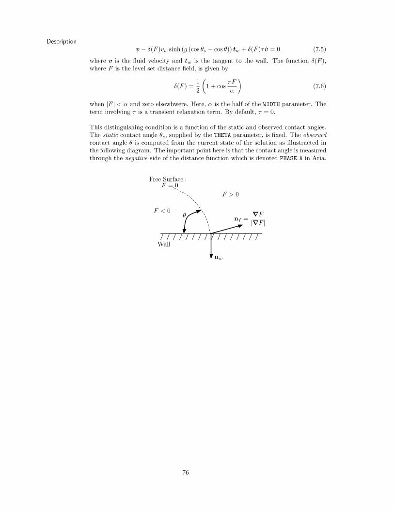
Descriptionv − δ(F )vw sinh (g (cos θs − cos θ)) tw + δ(F )τ v = 0 (7.5)
where v is the fluid velocity and tw is the tangent to the wall. The function δ(F ),where F is the level set distance field, is given by
δ(F ) =12
(1 + cos
πF
α
)(7.6)
when |F | < α and zero elsewhwere. Here, α is the half of the WIDTH parameter. Theterm involving τ is a transient relaxation term. By default, τ = 0.
This distinguishing condition is a function of the static and observed contact angles.The static contact angle θs, supplied by the THETA parameter, is fixed. The observedcontact angle θ is computed from the current state of the solution as illustracted inthe following diagram. The important point here is that the contact angle is measuredthrough the negative side of the distance function which is denoted PHASE A in Aria.
nw
!nf =
!F
|!F |
Free Surface :F = 0
Wall
F > 0
F < 0
76
Chapter 8
Source Terms
8.1 POINT SOURCE FOR . . .
Syntax POINT SOURCE FOR EQNAME ON MESH PART VALUE = Q X = x [Y = y [Z =z]]
Description Arbitrary point source contributions.
Details This adds a point source with value Q at the specified position. Currently limitedto constant and scalar sources. Only supported by the voltage equation (thoughextending it to other equations is simple, just ask). This line command syntax needsto change since the ON MESH PART piece doens’t really make sense since you alreadysupply the coordinates. You have to supply as many coordinate positions as theproblem has dimensions.
Mathematically, the point source is represented as
q = Qδ(x−X) (8.1)
where δ() is the Dirac delta function which is zero everywhwere except at the pointx = X where x is the physical coordinate and X is the position provided via theinput. In finite elements, this source is integrated∫
V
Qδ(x−X)φi dV = Qφi(X) ∈ ElemX . (8.2)
Here we employ the local support of the basis functions φ so that this is only evaluatedin the elements containing the point X, ElemX .
Parent Block(s) ARIA REGION
Example POINT SOURCE FOR Voltage ON block 1 Value = 1 X = 0 Y = 0 Z = 0
8.2 SOURCE FOR ENERGY
Syntax SOURCE FOR ENERGY ON MESH PART = MODEL [param1 = val1, param2 = val2
...]
77
Description Arbitrary source contributions for the energy equation.
Details Adds the source provided by MODEL to the energy equation.
Parent Block(s) ARIA REGION
8.2.1 SOURCE FOR ENERGY = VISCOUS DISSIPATION
Parameters [MULTIPLIER = REAL ]
Example Source For Energy on block 1 = Viscous Dissipation
Description This source accounts for the heat generation due to viscous dissipation:
q = m τ : ∇v (8.3)
where τ is the viscous stress tensor, ∇v is the gradient of the velocity and m is amultiplier (MULTIPLIER) that defaults to 1. The exact form of τ will depend on theMOMENTUM STRESS model choice(s) for the material.
8.2.2 SOURCE FOR ENERGY = COMPRESSIVE WORK
Parameters [MULTIPLIER = REAL ]
Example Source For Energy on block 1 = Compressive Work
Description This source accounts for the heat generation or consumption due to compression:
q = −m p : ∇ · v (8.4)
where p is the pressure, ∇ · v is the divergence of the velocity field and m is amultiplier (MULTIPLIER) that defaults to 1.
8.2.3 SOURCE FOR ENERGY = CURING FOAM HEAT OF RXN
Parameters VFRAC SUBINDEX = INT
EXTENT SUBINDEX = INT
H RXN = REAL
Example Source For Energy on block 1 = Curing Foam Heat of Rxn Vfrac Subindex=1Extent Subindex=2 H rxn=250
78
Description This source accounts for the heat of reaction of a curing epoxy foam, specifically:
q = ρ (1− φ) ∆Hrxn∂ξ
∂t(8.5)
where ρ is the density of the fluid, φ is the volume fraction, ∆Hrxn is the heat ofreaction and ξ is the extent of reaction.
NOTE: The volume fraction is assumed to be a SPECIES field with the subindexprovided by the VFRAC SUBINDEX parameter. Likewise, the extent of reaction field isassumed to be a SPECIES field with the subindex provided by the EXTENT SUBINDEXparameter.
8.2.4 SOURCE FOR ENERGY = CURING FOAM LATENT HEAT
Parameters VFRAC SUBINDEX = INT
H EVAP = REAL
Example Source For Energy on block 1 = Curing Foam Latent Heat Vfrac Subindex=1H evap=15
Description This source accounts for the loss of energy due to evaporation of a curing epoxy foam,specifically:
q = ρHevap∂φ
∂t(8.6)
where ρ is the density of the fluid, Hevap is the latent heat of evaporation and φ isthe volume fraction,
NOTE: The volume fraction is assumed to be a SPECIES field with the subindexprovided by the VFRAC SUBINDEX parameter.
8.2.5 SOURCE FOR ENERGY = CURING FOAM SPECIFIC HEAT
Parameters VFRAC SUBINDEX = INT
[CP FG = REAL ][CP E = REAL ][PHI ZERO = REAL ]
Example Source For Energy on block 1 = Curing Foam Specific HeatVfrac Subindex=1 Cp fG=1 Cp e=1 phi zero=0.2
79
Description This source accounts for the loss of energy due to the variable specific heat for the spe-cial case where the specific heat material model is CURING FOAM. See 10.32.2. Specif-ically, this source term is
q = −ρT
(∂Cp
∂t+ v · ∇Cp
)(8.7)
= −ρTb
(∂φ
∂t+ v · ∇φ
)(8.8)
where ρ is the density of the fluid, T is the temperature, v is the velocity, φ is thevolume fraction and b is as defined in CURING FOAM specific heat material model (see10.32.2).
NOTE: The volume fraction is assumed to be a SPECIES field with the subindexprovided by the VFRAC SUBINDEX parameter.
8.2.6 SOURCE FOR ENERGY = JOULE HEATING
Parameters [VOLTAGE SUBINDEX = INT ]
Example SOURCE FOR Energy ON block 1 = Joule Heating
Description This source term adds the volumetric heat source due to Joule heating, a.k.a., Ohmicheating or resitance heating. The volumetric heating is given by (see, Section 3.3)
HV = I2R (8.9)= (−σe∇V ) · (−σe∇V ) R (8.10)
= (−σe∇V ) · (−σe∇V )1σe
(8.11)
= σe (∇V · ∇V ) (8.12)
where I is the current density, R is the resitivity, σe = 1/R is the electrical conduc-tivity and V is the voltage.
8.2.7 SOURCE FOR ENERGY = POLYNOMIAL
Parameters VARIABLE = STRING
ORDER = INT
[C0 = REAL ][C1 = REAL ]...[CN = REAL ]
Example SOURCE For Energy on block 1 = Polynomial Variable=Temperature Order=1C0=401.0 C1=88.5
80
Description Arbitrary order polynomial function of a specified scalar variable.
HV =N∑
i=0
CiXi (8.13)
Here, N is the order of the polynomial provided by the ORDER parameter and X isthe variable supplied by the VARIABLE parameter and Ci are the supplied coefficients.Coefficients that are not supplied default to a value of zero. The VARIABLE argumentcan be TIME or any internal Expression that evaluates to a scalar. For the latter case,the format of the VARIABLE argument is described in section 2.6.1.
8.2.8 SOURCE FOR ENERGY = TBC JOULE HEATING
Parameters Ua = REAL
Ub = REAL
V NS = INT
Ti = REAL
CURRENT LOAD = REAL
[VOLTAGE SUBINDEX = INT ]
Example SOURCE FOR Energy ON block 1 = TBC Joule Heating Ua=1.4251 Ub=0.0004785V NS=1 Ti=298 CURRENT LOAD=0.0017
Description This source term adds the volumetric heat source due to Joule heating in a thermalbattery cell volumetric heating is given by (see, Section 3.3)
HV =(
U − V − Ti∂U∂T
)I (8.14)
Here, U is the open circuit potential which is given as a linear function in temperatureT and Ua and Ub are the coefficents of that function. V is the cell potential which istaken as the voltage at the node given in the single-node nodeset number V NS andI is cell load.
For more details, see Chen et al. (2000).
8.3 SOURCE FOR MOMENTUM
Syntax SOURCE FOR MOMENTUM ON MESH PART = MODEL [param1 = val1, param2 = val2
...]
Description Arbitrary source contributions for the momentum equation.
Details Adds the source provided by MODEL to the momentum equation.
Parent Block(s) ARIA REGION
81
8.3.1 SOURCE FOR MOMENTUM = CONSTANT VECTOR
Parameters [X = REAL ][Y = REAL ][Z = REAL ]
Example SOURCE FOR momentum ON block 1 = CONSTANT VECTOR Z=-9.8
Description This source term only applies to the momentum equation though it is automaticallyapplied to the continuity equation in PSPG formulations.
X, Y, Z are the components of the vector source. This vector source is not multipliedby the density.
8.3.2 SOURCE FOR MOMENTUM = HYDROSTATIC
Parameters GX = REAL
GY = REAL
GZ = REAL
[REF DENSITY = REAL ]
Example SOURCE FOR momentum ON block 1 = HYDROSTATIC gx = 0 gy = 0 gz = -980
Description This source term only applies to the momentum equation though it is automaticallyapplied to the continuity equation in PSPG formulations.
GX, GY, GZ are the components of the gravity vector g and REF DENSITY is an constant,uniform reference density ρ. With density ρ, the hydrostatic source is defined as(ρ− ρ)g.
The default value of the reference density is 0.
8.3.3 SOURCE FOR MOMENTUM = ROTATING BODY FORCE
Parameters G = REAL
FREQUENCY = REAL
[PHASE SHIFT = REAL ][REF DENSITY = REAL ]
Example Source for Momentum on block 1 = Rotating Body Force g=9.8frequency=2.5 phase shift=90
Description This source term only applies to the momentum equation though it is automaticallyapplied to the continuity equation in PSPG formulations.
GX, GY, GZ are the components of the gravity vector g and REF DENSITY is an constant,uniform reference density ρ. With density ρ, the hydrostatic source is defined as(ρ− ρ)g.
The default value of the reference density is 0.
82
8.3.4 SOURCE FOR MOMENTUM = BOUSSINESQ
Parameters TEMP REF = REAL
VOL EXP = REAL
GX = REAL
GY = REAL
GZ = REAL
Example SOURCE FOR momentum ON block 1 = BOUSSINESQ vol exp=0.1 temp ref=298.15gx = 0 gy = 0 gz = -980
Description This source term only applies to the momentum equation though it is automaticallyapplied to the continuity equation in PSPG formulations.
GX, GY, GZ are the components of the gravity vector g. VOL EXP is the volume expan-sion coefficient α and TEMP REF is the reference temperature Tref . With density ρand temperature T the Boussinesq source is defined as ρgα(T − Tref ).
8.4 SOURCE FOR CURRENT
Syntax SOURCE FOR CURRENT ON MESH PART = MODEL [param1 = val1, param2 = val2
...]
Description Arbitrary source contributions for the current equation.
Details Adds the source provided by MODEL to the current equation.
Parent Block(s) ARIA REGION
8.4.1 SOURCE FOR CURRENT = BUTLER VOLMER SIMPLE
Parameters A = REAL
C A = REAL
C C = REAL
U = REAL
Sign = INT
[V1 SUBINDEX = INT ][V2 SUBINDEX = INT ]
Example SOURCE FOR CURRENT 1 ON block 1 = Butler Volmer Simple A=1.0 C a=1.0C c=-1.0 U=0.2 Sign=-1SOURCE FOR CURRENT 2 ON block 1 = Butler Volmer Simple A=1.0 C a=1.0C c=-1.0 U=0.0 Sign=+1
83
Description This model implements a very simple form of the Butler-Volmer reaction kinetics. Itis intended for developmental and demonstrational purposes only.
This source term has the following form (see, also, equation 3.33)
RV,k = A(eca(V1−V2−U) − e−cc(V1−V2−U)
)(8.15)
where V1 is is the first electric potential field and V2 is the second electric potentialfield. By default V1 is VOLTAGE 1 and V2 is VOLTAGE 2 but the subindexes may bechanged using the optional V1 SUBINDEX and V2 SUBINDEX options.
8.4.2 SOURCE FOR CURRENT = POLYNOMIAL
Parameters VARIABLE = STRING
ORDER = INT
[C0 = REAL ][C1 = REAL ]...[CN = REAL ]
Example SOURCE For Current on block 1 = Polynomial Variable=TemperatureOrder=1 C0=401.0 C1=88.5
Description Arbitrary order polynomial function of a specified scalar variable.
HV =N∑
i=0
CiXi (8.16)
Here, N is the order of the polynomial provided by the ORDER parameter and X isthe variable supplied by the VARIABLE parameter and Ci are the supplied coefficients.Coefficients that are not supplied default to a value of zero. The VARIABLE argumentcan be TIME or any internal Expression that evaluates to a scalar. For the latter case,the format of the VARIABLE argument is described in section 2.6.1.
8.5 SOURCE FOR SPECIES
Syntax SOURCE FOR SPECIES ON MESH PART = MODEL [param1 = val1, param2 = val2
...]
Description Arbitrary source contributions for the species equation.
Details Adds the source provided by MODEL to the current equation.
Parent Block(s) ARIA REGION
84
8.5.1 SOURCE FOR SPECIES = CURING FOAM EXTENT
Parameters K = REAL
E = REAL
R = REAL
N = REAL
Example Source For Species 2 on block 1 = Curing Foam Extent k=1.145e5 E=10R=8.314472E3 n=1.3
Description This source accounts for the reaction of a curing epoxy foam, specifically:
q = keE/RT (1− ξ)n (8.17)
where T is the temperature and ξ is the extent of reaction.
8.5.2 SOURCE FOR SPECIES = CURING FOAM VFRAC
Parameters A = REAL
B = REAL
C = REAL
T BOILING = REAL
Example Source For Species 2 on block 1 = Curing Foam Vfrac a=1 b=0 c=2e-3T BOILING=473.15
Description This source accounts for the change in volume fraction with temperature.
q =(a + bT + cT 2
)exp
∂T
∂t(8.18)
where T is the temperature. This source term is only active when T >= Tboiling.
8.5.3 SOURCE FOR SPECIES = POLYNOMIAL
Parameters VARIABLE = STRING
ORDER = INT
[C0 = REAL ][C1 = REAL ]...[CN = REAL ]
Example Source For Species on block 1 = Polynomial Variable=TemperatureOrder=1 C0=401.0 C1=88.5
85
Description Arbitrary order polynomial function of a specified scalar variable.
HV =N∑
i=0
CiXi (8.19)
Here, N is the order of the polynomial provided by the ORDER parameter and X isthe variable supplied by the VARIABLE parameter and Ci are the supplied coefficients.Coefficients that are not supplied default to a value of zero. The VARIABLE argumentcan be TIME or any internal Expression that evaluates to a scalar. For the latter case,the format of the VARIABLE argument is described in section 2.6.1.
8.6 SOURCE FOR VOLTAGE
Syntax SOURCE FOR VOLTAGE ON MESH PART = MODEL [param1 = val1, param2 = val2
...]
Description Arbitrary source contributions for the voltage equation.
Details Adds the source provided by MODEL to the current equation.
Parent Block(s) ARIA REGION
8.6.1 SOURCE FOR VOLTAGE = POLYNOMIAL
Parameters VARIABLE = STRING
ORDER = INT
[C0 = REAL ][C1 = REAL ]...[CN = REAL ]
Example Source For Voltage on block 1 = Polynomial Variable=TemperatureOrder=1 C0=401.0 C1=88.5
Description Arbitrary order polynomial function of a specified scalar variable.
HV =N∑
i=0
CiXi (8.20)
Here, N is the order of the polynomial provided by the ORDER parameter and X isthe variable supplied by the VARIABLE parameter and Ci are the supplied coefficients.Coefficients that are not supplied default to a value of zero. The VARIABLE argumentcan be TIME or any internal Expression that evaluates to a scalar. For the latter case,the format of the VARIABLE argument is described in section 2.6.1.
86
Chapter 9
Constraint Conditions
9.1 CONSTRAIN
Syntax CONSTRAIN AVERAGE VOLUME FRACTION phi = C0
Description Integral constraint for the average particle volume fraction in a SUSPENSION prob-lem.
Details Constrains φ throughout the problem domain to achieve the specified value of averagevolume particle fraction in accordance with the relation
C0 =
[∫Vφ
dV
]−1 ∫Vφ
φdV (9.1)
over element blocks where the SUSPENSION equation is defined.
Parent Block(s) ARIA REGION
87

88
Chapter 10
Material Properties
10.1 BETA
Syntax BETA = MODEL [param1 = val1, param2 = val2 ...]
Description Specifies the coefficient for thermal stress.
Details The solid stress T is given by
T = λEkkI + 2µE − β (T − Tref ) I (10.1)
where λ and µ are the Lame coefficients, E = 12
(∇d + ∇dT
)is the deformation
tensor, β is the coefficient of thermal stress, T is temperature and Tref is the solidstress reference temperature.
These Lame coefficients are related to the more standard Young’s modulus, Poisson’sratio and CTE (α) as follows:
2µ =E
(1 + ν)(10.2)
λ =νE
(1 + ν) (1− 2ν)= 2µ
ν
(1− 2ν)(10.3)
β =αE
(1− 2ν)= α (3λ + 2µ) (10.4)
When a user supplies the Young’s modulus, Poisson’s ratio and CTE properties Ariainternally convertes them into the Lame coefficients.
Parent Block(s) ARIA MATERIAL
10.1.1 BETA = CONSTANT
Parameters BETA = REAL
Example BETA = CONSTANT BETA = 1.0
89
Description BETA is the value of β.
10.1.2 BETA = CONVERTED
Parameters (None)
Example BETA = Converted
Description Aria will use Young’s modulus, Poisson ratio and CTE to compute the Lame β coeffi-cient. Supplying the Lame coefficients is more computationally efficient but perhapsless convenient, especially if the material properties are varying (e.g., temperaturedependent in a non-isothermal problem).
10.1.3 BETA = LINEAR
Parameters A = REAL
B = REAL
Example BETA = LINEAR A = 1.0 B = -.005
Description β is a inear function of temperature T ,
β = A + BT (10.5)
10.2 BULK VISCOSITY
Syntax BULK VISCOSITY = MODEL [param1 = val1, param2 = val2 ...]
Description Specifies the material model for the fluid bulk viscosity.
Details Specifies the material model for the fluid bulk viscosity.
Parent Block(s) ARIA MATERIAL
10.2.1 BULK VISCOSITY = CONSTANT
Parameters KAPPA = REAL
90
Example BULK VISCOSITY = CONSTANT KAPPA = 1.0e-5
Description KAPPA is the value of the constant fluid bulk viscosity.
10.2.2 BULK VISCOSITY = CURING FOAM
Parameters VFRAC SUBINDEX = INT
EXTENT SUBINDEX = INT
PHI ZERO = REAL
[A = REAL ][B = REAL ][C = REAL ][KSI C = REAL ]
Example Bulk Viscosity = Curing Foam Vfrac Subindex=1 Extent Subindex=2Phi Zero=0.45
Description For a curing expoxy with volume fraction φ and extent of reaction ξ the viscosity isgiven by
κ =43µ
φ − φ− 1φ − φ
(10.6)
where µ is given by
µ = (a− bT )(
ξ2c − ξ2
ξ2c
)c
(10.7)
where T is the tempature. The remaining parameters a, b, c and ξc have defaultvalues of a = 20, b = 0.22, c = −4/3 and ξc = 0.45 though they can be overriddenwith the optional model parameters.
NOTE: The volume fraction is assumed to be a SPECIES field with the subindexprovided by the VFRAC SUBINDEX parameter. Likewise, the extent of reaction field isassumed to be a SPECIES field with the subindex provided by the EXTENT SUBINDEXparameter.
10.3 CTE
Syntax CTE = MODEL [param1 = val1, param2 = val2 ...]
Description Specifies the coefficient of thermal expansion.
91
Details The solid stress T is given by
T = λEkkI + 2µE − β (T − Tref ) I (10.8)
where λ and µ are the Lame coefficients, E = 12
(∇d + ∇dT
)is the deformation
tensor, β is the coefficient of thermal stress, T is temperature and Tref is the solidstress reference temperature.
These Lame coefficients are related to the more standard Young’s modulus, Poisson’sratio and CTE (α) as follows:
2µ =E
(1 + ν)(10.9)
λ =νE
(1 + ν) (1− 2ν)= 2µ
ν
(1− 2ν)(10.10)
β =αE
(1− 2ν)= α (3λ + 2µ) (10.11)
When a user supplies the Young’s modulus, Poisson’s ratio and CTE properties Ariainternally convertes them into the Lame coefficients.
Supplying the Lame coefficients is more computationally efficient but perhaps lessconvenient, especially if the material properties are varying (e.g., temperature depen-dent in a non-isothermal problem).
Parent Block(s) ARIA MATERIAL
10.3.1 CTE = CONSTANT
Parameters CTE = REAL
Example CTE = CONSTANT cte = 1.0
Description CTE is the value of the coefficient of thermal expansion.
10.4 CURRENT DENSITY
Syntax CURRENT DENSITY = MODEL [param1 = val1, param2 = val2 ...]
Description Specifies the material (constitutive) model for the current density in the bulk.
Details Specifies the material (constitutive) model for the current density in the bulk.
92
Parent Block(s) ARIA MATERIAL
10.4.1 CURRENT DENSITY = BASIC
This is an alias for OHMS LAW.
Example Current Density = Basic
10.4.2 CURRENT DENSITY = OHMS LAW
Parameters (none)
Example Current Density = Ohms Law
Description The current density J is given by Ohm’s Law,
J = −σe∇V (10.12)
where σe is the electrical conducitivity and V is the voltage (electric potential).
10.5 DENSITY
Syntax DENSITY = MODEL [param1 = val1, param2 = val2 ...]
Description Specifies the material model for the density.
Details Specifies the material model for the density.
Parent Block(s) ARIA MATERIAL
10.5.1 DENSITY = CONSTANT
Parameters RHO = REAL
Example DENSITY = CONSTANT RHO = 1.0
Description RHO is the value of the constant density.
93
10.5.2 DENSITY = CURING FOAM
Parameters R = REAL
RHO E = REAL
RHO F = REAL
PHI ZERO = REAL
VFRAC SUBINDEX = INT
Example Molecular Weight = Constant Subindex=1 M = 17.0Density = Curing Foam R=8.314472E3 RHO E=1 RHO F=1.5 PHI ZERO=0.2VFRAC SUBINDEX=1
Description The density curing epoxy foam with volume fraction φ, molecular weight M , temper-ature T , and pressure p is given by
ρ = (φ − φ)pM
RT+ (1− φ) ρe + φρf (10.13)
where R is the gas constant, φ is the reference volume fraction in the flourinert ρe
is the pure expoxy density and ρf is the pure flourinert density.
NOTE: The volume fraction is assumed to be a SPECIES field with the subindexprovided by the VFRAC SUBINDEX parameter.
10.5.3 DENSITY = EXP DECAY
Parameters RHO INITIAL = REAL
RHO FINAL = REAL
K = REAL
Example Density = Exp Decay K=1.2 RHO INITIAL=1.0 RHO FINAL=0.2
Description This model supplies a density that is an exponential decay,
ρ = ρf + (ρi − ρf ) e−kt (10.14)
where ρi is the initial density (RHO INITIAL), ρf is the final density (RHO FINAL andk (K) is the decay constant.
10.5.4 DENSITY = IDEAL GAS
Parameters R = REAL
[P REF = REAL ][T REF = REAL ]
Example Molecular Weight = Constant Subindex=1 M = 17.0Molecular Weight = Constant Subindex=2 M = 23.0Density = Ideal Gas R=8.314472E3 T ref=273.15 P ref=101325.0
94
Description The density of a multicomponent ideal gas in kg m−3 may be written as
ρ =Pref + P
R (Tref + T )
N∑i
Miyi (10.15)
where N is the number of species, P is the pressure in Pascals, Pref is a referencepressure, R is the gas constant, T is the temperature, Tref is a reference temperature,Mi is the molecular weight of species i in kg kmol−1 and yi is the mole fraction ofspecies i. Note, the units given here and on the density card are si units; any unitsmay be used as long as internal consistency is maintained.
The optional reference values for the temperature and pressure allow you to solvefor the temperature and pressure using relative units (e.g., Celcius temperature andgauge pressure) and but still use absolute values as required by this material model.
10.5.5 DENSITY = INCOMPRESSIBLE IDEAL GAS
Parameters R = REAL
P REF = REAL
[T REF = REAL ]
Example Molecular Weight = Constant Subindex=1 M = 17.0Molecular Weight = Constant Subindex=2 M = 23.0Density = Incompressible Ideal Gas R=8.314472E3 T ref=273.15P ref=101325.0
Description The density of a multicomponent ideal gas in kg m−3 may be written as
ρ =Pref
R (Tref + T )
N∑i
Miyi (10.16)
where N is the number of species, Pref is a reference pressure in pascal, R is the gasconstant in J kmol−1 K−1, T is the temperature, Tref is a reference temperature,Mi is the molecular weight of species i in kg kmol−1, and yi is the mole fraction ofspecies i. Note, the units given here and on the density card are si units; any unitsmay be used as long as internal consistency is maintained.
The optional reference value for the temperature allow you to solve for the tempera-ture using relative units (e.g., Celcius temperature) and but still use absolute valuesas required by this material model.
10.5.6 DENSITY = POLYNOMIAL
Parameters VARIABLE = STRING
ORDER = INT
[C0 = REAL ][C1 = REAL ]...[CN = REAL ]
Example Density = Polynomial Variable=Temperature Order=1 C0=401.0 C1=88.5
95
Description Arbitrary order polynomial function of a specified scalar variable.
ρ =N∑
i=0
CiXi (10.17)
Here, N is the order of the polynomial provided by the ORDER parameter and X isthe variable supplied by the VARIABLE parameter and Ci are the supplied coefficients.Coefficients that are not supplied default to a value of zero. The VARIABLE argumentcan be TIME or any internal Expression that evaluates to a scalar. For the latter case,the format of the VARIABLE argument is described in section 2.6.1.
10.5.7 DENSITY = THERMAL
Parameters [A = REAL ][B = REAL ][C = REAL ][D = REAL ]
Example DENSITY = THERMAL A = 1.0 B = -.005
Description Cubic polynomial function of temperature for the density.
ρ = A + BT + CT 2 + DT 3 (10.18)
10.5.8 DENSITY = USER FUNCTION
Parameters NAME = STRING
X = STRING
96
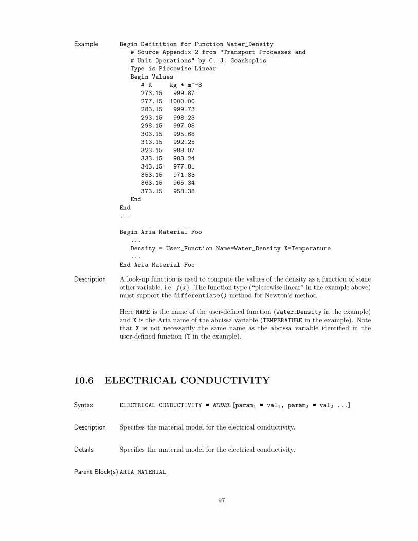
Example Begin Definition for Function Water_Density# Source Appendix 2 from "Transport Processes and# Unit Operations" by C. J. GeankoplisType is Piecewise LinearBegin Values
# K kg * m^-3273.15 999.87277.15 1000.00283.15 999.73293.15 998.23298.15 997.08303.15 995.68313.15 992.25323.15 988.07333.15 983.24343.15 977.81353.15 971.83363.15 965.34373.15 958.38
EndEnd...
Begin Aria Material Foo...Density = User_Function Name=Water_Density X=Temperature...
End Aria Material Foo
Description A look-up function is used to compute the values of the density as a function of someother variable, i.e. f(x). The function type (“piecewise linear” in the example above)must support the differentiate() method for Newton’s method.
Here NAME is the name of the user-defined function (Water Density in the example)and X is the Aria name of the abcissa variable (TEMPERATURE in the example). Notethat X is not necessarily the same name as the abcissa variable identified in theuser-defined function (T in the example).
10.6 ELECTRICAL CONDUCTIVITY
Syntax ELECTRICAL CONDUCTIVITY = MODEL [param1 = val1, param2 = val2 ...]
Description Specifies the material model for the electrical conductivity.
Details Specifies the material model for the electrical conductivity.
Parent Block(s) ARIA MATERIAL
97
10.6.1 ELECTRICAL CONDUCTIVITY = CONSTANT
Parameters SIGMA = REAL
Example ELECTRICAL CONDUCTIVITY = CONSTANT SIGMA = 1.0
Description SIGMA is the value of the constant electrical conductivity.
10.6.2 ELECTRICAL CONDUCTIVITY = EXPONENTIAL
Parameters VARIABLE = STRING
[CONSTANT = REAL ][MULTIPLIER = REAL ]EXPONENT = REAL
Example Electrical Conductivity = Exponential Variable=TemperatureMultiplier=1.0 Exponent=-0.3
Description Exponential function of in specified scalar variable. The electrical conductivity iscomputed as
σe = C + MeEX (10.19)
Here, C is the constant term supplied by the CONSTANT parameter which defaults tozero, M is the value supplied by the MULTIPLIER parameter which defaults to unity,X is the variable supplied by the VARIABLE parameter and E is the exponentialmultiplier provided by the EXPONENT parameter.
10.6.3 ELECTRICAL CONDUCTIVITY = FROM RESISTANCE
Parameters None.
Example ELECTRICAL CONDUCTIVITY = FROM RESISTANCE
Description The conductivity is computed as the inverse of the electrical resistance which mustbe provided separately.
10.6.4 ELECTRICAL CONDUCTIVITY = POLYNOMIAL
Parameters VARIABLE = STRING
ORDER = INT
[C0 = REAL ][C1 = REAL ]...[CN = REAL ]
Example Electrical Conductivity = Polynomial Variable=Temperature Order=1C0=401.0 C1=88.5
98
Description Arbitrary order polynomial function of a specified scalar variable.
σe =N∑
i=0
CiXi (10.20)
Here, N is the order of the polynomial provided by the ORDER parameter and X isthe variable supplied by the VARIABLE parameter and Ci are the supplied coefficients.Coefficients that are not supplied default to a value of zero. The VARIABLE argumentcan be TIME or any internal Expression that evaluates to a scalar. For the latter case,the format of the VARIABLE argument is described in section 2.6.1.
10.6.5 ELECTRICAL CONDUCTIVITY = TBC
Parameters Ki = REAL
Ti = REAL
E = REAL
R = REAL
Example ELECTRICAL CONDUCTIVITY = TBC Ki=1.0 Ti=273 R=8.314 E=1e-3
Description Thermal battery electrical conductivity model (see Ken Chen).
κ(T ) = κiTi
Te−E
R
“1T −
1Ti
”(10.21)
Here, T is temperature, Ti is the initial temperature provided by Ti, κi is the electricalconductivity at Ti provided by Ki, R is the universal gas constant provided by R andE is the energy provided by E.
10.6.6 ELECTRICAL CONDUCTIVITY = THERMAL
Parameters [A = REAL ][B = REAL ][C = REAL ][D = REAL ]
Example ELECTRICAL CONDUCTIVITY = THERMAL A = 1.0 B = -0.01
Description Cubic polynomial function of temperature for the conductivity.
σe = A + BT + CT 2 + DT 3 (10.22)
10.7 ELECTRIC DISPLACEMENT
Syntax ELECTRIC DISPLACEMENT = MODEL [param1 = val1, param2 = val2 ...]
99
Description Specifies the material (constitutive) model for the electric displacement
Details Specifies the material (constitutive) model for the electric displacement
Parent Block(s) ARIA MATERIAL
10.7.1 ELECTRIC DISPLACEMENT = BASIC
This is an alias for LINEAR.
Example Electric Displacement = Basic
10.7.2 ELECTRIC DISPLACEMENT = LINEAR
Parameters (none)
Example Electric Displacement = Linear
Description The electric displacement D is linearly proportional to the electric field (E = −∇V )
D = −ε∇V (10.23)
where ε is the electrical permittivity and V is the voltage (electric potential).
10.8 ELECTRICAL PERMITTIVITY
Syntax ELECTRICAL PERMITTIVITY = MODEL [param1 = val1, param2 = val2 ...]
Description Specifies the material model for the electrical permittivity.
Details Specifies the material model for the electrical permittivity.
Parent Block(s) ARIA MATERIAL
10.8.1 ELECTRICAL PERMITTIVITY = CONSTANT
Parameters E = REAL
100
Example ELECTRICAL PERMITTIVITY = CONSTANT E = 1.0
Description E is the value of the constant electrical permittivity.
10.9 ELECTRICAL RESISTANCE
Syntax ELECTRICAL RESISTANCE = MODEL [param1 = val1, param2 = val2 ...]
Description Specifies the material model for the electrical resistance.
Details Specifies the material model for the electrical resistance.
Parent Block(s) ARIA MATERIAL
10.9.1 ELECTRICAL RESISTANCE = CONSTANT
Parameters None.
Example ELECTRICAL RESISTANCE = CONSTANT R = 1.0
Description R is the value of the constant electrical resistance.
10.9.2 ELECTRICAL RESISTANCE = EXPONENTIAL
Parameters VARIABLE = STRING
[CONSTANT = REAL ][MULTIPLIER = REAL ]EXPONENT = REAL
Example Electrical Resistance = Exponential Variable=TemperatureMultiplier=1.0 Exponent=-0.3
Description Exponential function of in specified scalar variable. The electrical resistance is com-puted as
R = C + MeEX (10.24)
Here, C is the constant term supplied by the CONSTANT parameter which defaults tozero, M is the value supplied by the MULTIPLIER parameter which defaults to unity,X is the variable supplied by the VARIABLE parameter and E is the exponentialmultiplier provided by the EXPONENT parameter.
101
10.9.3 ELECTRICAL RESISTANCE = FROM CONDUCTIVITY
Parameters R = REAL
Example ELECTRICAL RESISTANCE = FROM CONDUCTIVITY
Description The resistance is computed as the inverse of the electrical conductivity which mustbe provided separately.
10.9.4 ELECTRICAL RESISTANCE = POLYNOMIAL
Parameters VARIABLE = STRING
ORDER = INT
[C0 = REAL ][C1 = REAL ]...[CN = REAL ]
Example Electrical Resistance = Polynomial Variable=Temperature Order=1C0=401.0 C1=88.5
Description Arbitrary order polynomial function of a specified scalar variable.
R =N∑
i=0
CiXi (10.25)
Here, N is the order of the polynomial provided by the ORDER parameter and X isthe variable supplied by the VARIABLE parameter and Ci are the supplied coefficients.Coefficients that are not supplied default to a value of zero. The VARIABLE argumentcan be TIME or any internal Expression that evaluates to a scalar. For the latter case,the format of the VARIABLE argument is described in section 2.6.1.
10.9.5 ELECTRICAL RESISTANCE = USER FUNCTION
Parameters NAME = STRING
X = STRING
102
Example Begin definition for function RESISTANCE_DATAType is piecewise linearAbscissa is TOrdinate is Electrical_ResistanceBegin Values
# [K] [Ohm-um]273 1.00E-9323 7.99E-10...873 1.09E-11
End ValuesEnd definition for function RESISTANCE_DATA
...
Begin Aria Material Foo...Electrical Resistance = User_Function Name=RESISTANCE_DATA X=Temperature...
End Aria Material Foo
Description A look-up function is used to compute the values of the resistance as a function ofsome other variable, i.e. f(x). The function type (“piecewise linear” in the exampleabove) must support the differentiate() method for Newton’s method.
Here NAME is the name of the user-defined function (RESISTANCE DATA in the example)and X is the Aria name of the abcissa variable (TEMPERATURE in the example). Notethat X is not necessarily the same name as the abcissa variable identified in theuser-defined function (T in the example).
10.10 EMISSIVITY
Syntax EMISSIVITY = MODEL [param1 = val1, param2 = val2 ...]
Description Specifies the material model for the emissivity.
Details Specifies the material model for the emissivity.
Parent Block(s) ARIA MATERIAL
10.10.1 EMISSIVITY = CONSTANT
Parameters E = REAL
Example Emissivity = Constant E = 0.8
103
Description E is the value of the constant emissivity.
10.11 ENTHALPHY
Syntax ENTHALPHY = MODEL [param1 = val1, param2 = val2 ...]
Description Specifies a model for the enthalphy of a material.
Details Specifies a model for the enthalphy of a material.
Parent Block(s) ARIA MATERIAL
10.11.1 ENTHALPHY = CONSTANT
Parameters H = REAL
Example Enthalphy = Constant H=1e-4
Description The value is constant in space and time.
10.12 EQUATION OF STATE
Syntax EQUATION OF STATE = MODEL [param1 = val1, param2 = val2 ...]
Description Specifies the equation of state for gas dynamics problems.
Details Specifies the equation of state for gas dynamics problems.
Parent Block(s) ARIA MATERIAL
10.12.1 EQUATION OF STATE = IDEAL GAS
Parameters R = REAL
GAMMA = REAL
Example Equation of State = Ideal Gas R=8.314 Gamma=1.4
104
Description R is the gas constant and GAMMA is the ratio of heat capacities.
This model is used for gas dynamics problems where the density is an unknown. Inthis case, the pressure is given by the ideal gas law,
p = RTρ (10.26)
where T is the temperature and ρ is the density. Activating this model supplies severalquantities that are related to this equation of state such as the pressure, temperature,and other gas dynamics related quantities.
10.13 HEAT CONDUCTION
Syntax HEAT CONDUCTION = MODEL [param1 = val1, param2 = val2 ...]
Description Specifies the material (constitutive) model for the heat conduction (diffusive flux) inthe bulk.
Details Specifies the material (constitutive) model for the heat conduction (diffusive flux) inthe bulk.
Parent Block(s) ARIA MATERIAL
10.13.1 HEAT CONDUCTION = BASIC
This is an alias for FOURIERS LAW.
Example Heat Conduction = Basic
10.13.2 HEAT CONDUCTION = CONVECTED ENTHALPY
Parameters (none)
Example Heat Conduction = Convected Enthalpy
Description The heat conduction (flux) q is given by,
q = −hρv (10.27)
where h is the enthalpy, ρ is the density and v is the velocity.
10.13.3 HEAT CONDUCTION = FOURIERS LAW
Parameters (none)
105
Example Heat Conduction = Fouriers Law
Description The heat conduction (flux) q is given by Fourier’s Law,
q = −κ∇T (10.28)
where κ is the thermal conductivity and T is the temperature.
10.14 HEAT OF VAPORIZATION
Syntax HEAT OF VAPORIZATION = MODEL [param1 = val1, param2 = val2 ...]
Description Specifies the heat of vaporization for a material or for a particular species.
Details Quantifies the amount of energy consumed during evaporation per unit mass.
Parent Block(s) ARIA MATERIAL
10.14.1 HEAT OF VAPORIZATION = CONSTANT
Parameters Hv = REAL
[SUBINDEX = INT ]
Example HEAT OF VAPORIZATION = CONSTANT SUBINDEX=0 Hv = 1.0HEAT OF VAPORIZATION = CONSTANT SUBINDEX=1 Hv = 2.0HEAT OF VAPORIZATION = CONSTANT SUBINDEX=3 Hv = 3.14
Description HV is the value of the constant heat of vaporization and SUBINDEX is the optioinalspecies index (used in multicomponent systems).
10.15 INTRINSIC PERMEABILITY
Syntax INTRINSIC PERMEABILITY = MODEL [param1 = val1, param2 = val2 ...]
Description Specifies the material model for the intrinsic permeability tensor for porous flow inDarcy’s Law.
106
Details Specifies the material model for the intrinsic permeability tensor for porous flow inDarcy’s Law. In general, the permeability may be nonisotropic in porour media. Inthat case, Darcy’s law may be written as,
ρvd = f = −ρkr
µK · (∇P − ρg) (10.29)
where K is the intrinsic permeability tensor, ρ is the density, vd is the Darcy velocity,f is the mas flux, kr is the relative permeability, P is pressure and g is gravity.
Parent Block(s) ARIA MATERIAL
10.15.1 INTRINSIC PERMEABILITY = CONSTANT
Parameters [XX = REAL ][XY = REAL ][XZ = REAL ][YX = REAL ][YY = REAL ][YZ = REAL ][ZX = REAL ][ZY = REAL ][ZZ = REAL ]
Example Intrinsic Permeability = Constant XX=1 YY=2 ZZ=1
Description All components default to zero and all values are constant in space and time.
10.16 INTERNAL ENERGY
Syntax INTERNAL ENERGY = MODEL [param1 = val1, param2 = val2 ...]
Description Specifies a model for the internal energy of a material.
Details Specifies a model for the internal of a material.
Parent Block(s) ARIA MATERIAL
10.16.1 INTERNAL ENERGY = GAS PHASE
Parameters (none)
Example Internal Energy = Gas Phase
107
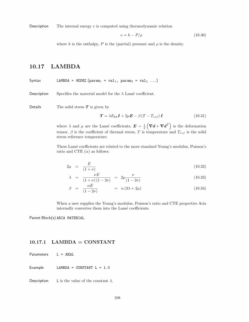
Description The internal energy e is computed using thermodynamic relation
e = h− P/ρ (10.30)
where h is the enthalpy, P is the (partial) pressure and ρ is the density.
10.17 LAMBDA
Syntax LAMBDA = MODEL [param1 = val1, param2 = val2 ...]
Description Specifies the material model for the λ Lame coefficient.
Details The solid stress T is given by
T = λEkkI + 2µE − β (T − Tref ) I (10.31)
where λ and µ are the Lame coefficients, E = 12
(∇d + ∇dT
)is the deformation
tensor, β is the coefficient of thermal stress, T is temperature and Tref is the solidstress reference temperature.
These Lame coefficients are related to the more standard Young’s modulus, Poisson’sratio and CTE (α) as follows:
2µ =E
(1 + ν)(10.32)
λ =νE
(1 + ν) (1− 2ν)= 2µ
ν
(1− 2ν)(10.33)
β =αE
(1− 2ν)= α (3λ + 2µ) (10.34)
When a user supplies the Young’s modulus, Poisson’s ratio and CTE properties Ariainternally convertes them into the Lame coefficients.
Parent Block(s) ARIA MATERIAL
10.17.1 LAMBDA = CONSTANT
Parameters L = REAL
Example LAMBDA = CONSTANT L = 1.0
Description L is the value of the constant λ.
108
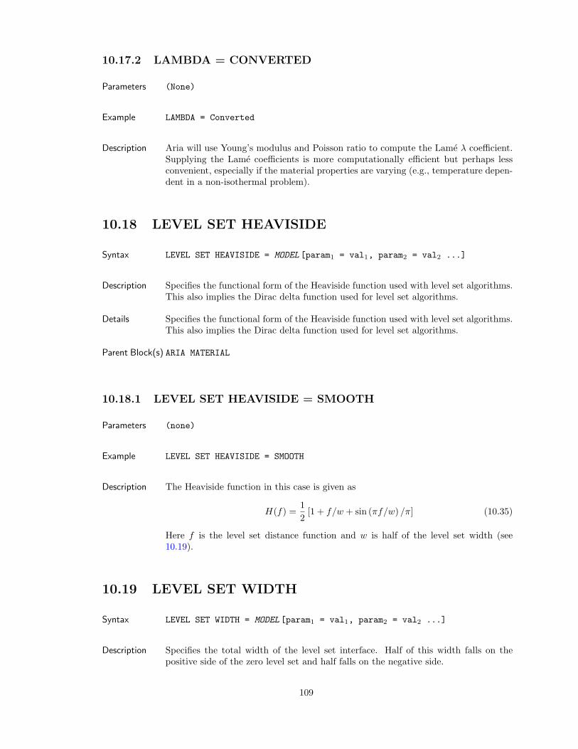
10.17.2 LAMBDA = CONVERTED
Parameters (None)
Example LAMBDA = Converted
Description Aria will use Young’s modulus and Poisson ratio to compute the Lame λ coefficient.Supplying the Lame coefficients is more computationally efficient but perhaps lessconvenient, especially if the material properties are varying (e.g., temperature depen-dent in a non-isothermal problem).
10.18 LEVEL SET HEAVISIDE
Syntax LEVEL SET HEAVISIDE = MODEL [param1 = val1, param2 = val2 ...]
Description Specifies the functional form of the Heaviside function used with level set algorithms.This also implies the Dirac delta function used for level set algorithms.
Details Specifies the functional form of the Heaviside function used with level set algorithms.This also implies the Dirac delta function used for level set algorithms.
Parent Block(s) ARIA MATERIAL
10.18.1 LEVEL SET HEAVISIDE = SMOOTH
Parameters (none)
Example LEVEL SET HEAVISIDE = SMOOTH
Description The Heaviside function in this case is given as
H(f) =12
[1 + f/w + sin (πf/w) /π] (10.35)
Here f is the level set distance function and w is half of the level set width (see10.19).
10.19 LEVEL SET WIDTH
Syntax LEVEL SET WIDTH = MODEL [param1 = val1, param2 = val2 ...]
Description Specifies the total width of the level set interface. Half of this width falls on thepositive side of the zero level set and half falls on the negative side.
109
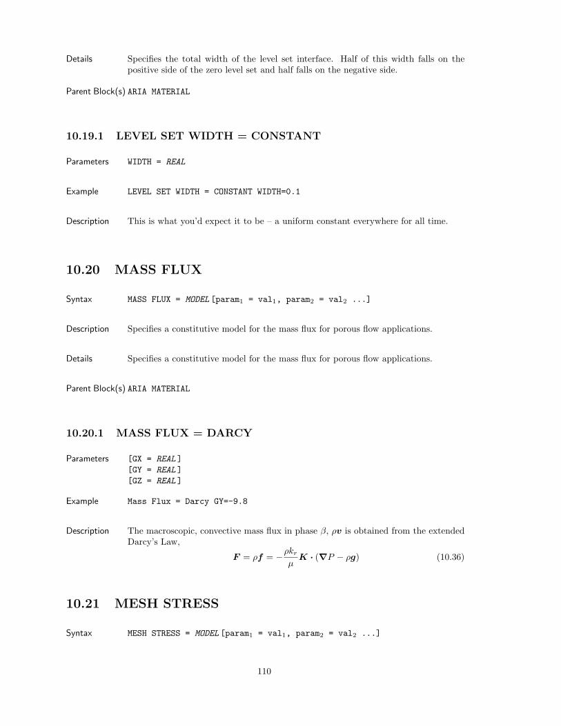
Details Specifies the total width of the level set interface. Half of this width falls on thepositive side of the zero level set and half falls on the negative side.
Parent Block(s) ARIA MATERIAL
10.19.1 LEVEL SET WIDTH = CONSTANT
Parameters WIDTH = REAL
Example LEVEL SET WIDTH = CONSTANT WIDTH=0.1
Description This is what you’d expect it to be – a uniform constant everywhere for all time.
10.20 MASS FLUX
Syntax MASS FLUX = MODEL [param1 = val1, param2 = val2 ...]
Description Specifies a constitutive model for the mass flux for porous flow applications.
Details Specifies a constitutive model for the mass flux for porous flow applications.
Parent Block(s) ARIA MATERIAL
10.20.1 MASS FLUX = DARCY
Parameters [GX = REAL ][GY = REAL ][GZ = REAL ]
Example Mass Flux = Darcy GY=-9.8
Description The macroscopic, convective mass flux in phase β, ρv is obtained from the extendedDarcy’s Law,
F = ρf = −ρkr
µK · (∇P − ρg) (10.36)
10.21 MESH STRESS
Syntax MESH STRESS = MODEL [param1 = val1, param2 = val2 ...]
110
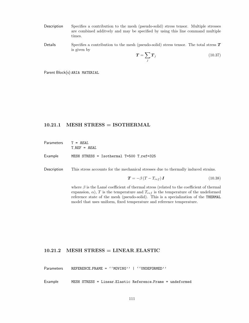
Description Specifies a contribution to the mesh (pseudo-solid) stress tensor. Multiple stressesare combined additvely and may be specified by using this line command multipletimes.
Details Specifies a contribution to the mesh (pseudo-solid) stress tensor. The total stress Tis given by
T =∑
j
T j (10.37)
Parent Block(s) ARIA MATERIAL
10.21.1 MESH STRESS = ISOTHERMAL
Parameters T = REAL
T REF = REAL
Example MESH STRESS = Isothermal T=500 T ref=325
Description This stress accounts for the mechanical stresses due to thermally induced strains.
T = −β (T − Tref ) I (10.38)
where β is the Lame coefficient of thermal stress (related to the coefficient of thermalexpansion, α), T is the temperature and Tref is the temperature of the undeformedreference state of the mesh (pseudo-solid). This is a specialization of the THERMALmodel that uses uniform, fixed temperature and reference temperature.
10.21.2 MESH STRESS = LINEAR ELASTIC
Parameters REFERENCE FRAME = ‘‘MOVING’’ | ‘‘UNDEFORMED’’
Example MESH STRESS = Linear Elastic Reference Frame = undeformed
111
Description Supplies the linear elasticity stress tensor,
T = λ trace EI + 2µE (10.39)
where λ and µ and the Lame coefficients and E is the strain tensor. When thechoice of refernce frame is “UNDEFORMED” then the strain is computed in theundeformed reference state; this is commonly referred to as small strain theory. Whenthe reference frame is “MOVING” then the strain is computed with respect to thedeformed coordinates.
Specifically, the strain tensor is given by
E =12(∇d + ∇dt
)(10.40)
where d is the mesh displacement field. The choice of reference frame determineswhether the ∇ operator is computed in the undeformed or moving reference frames.
10.21.3 MESH STRESS = NEOHOOKEAN ELASTIC
Parameters (none)
Example MESH STRESS = Neohookean Elastic
Description Supplies a nonlinear hyperelastic stress of the form,
T =µ
J(b− I) +
λ
JlnJI (10.41)
where λ and µ and the Lame coefficients, b ≡ F ·F t is the left Cauchy-Green tensor,F is the deformation gradient and J ≡ det F . See, e.g., Bonet and Wood (1997) orBelytschko et al. (2004).
10.21.4 MESH STRESS = NONLINEAR ELASTIC
Parameters (none)
Example MESH STRESS = Nonlinear Elastic
Description Supplies a nonlinear elastic stress,
T = λ trace EI + 2µE (10.42)
where λ and µ and the Lame coefficients and E is the strain tensor. The particularchoice of strain tensor chosen depends on where the configuration (reference frame)which is set via the MESH MOTION command line. See section 3.11 for moreinformation. When the MESH MOTION is set to ARBITRARY then the Greenstrain is used. Otherwise, the Almansi strain is used.
112
10.21.5 MESH STRESS = RESIDUAL
Parameters [SXX | SX = REAL ][SYY | SY = REAL ][SZZ | SZ = REAL ][SXY = REAL ][SXZ = REAL ][SYZ = REAL ]
Example SOLID STRESS = Residual Sxx=0.02 Syy=0.02
Description This stress accounts for the initial residual stress in a solid that is constant anduniform everywhere. The components of the residual stress tensor are supplied bythe (up-to) six components SXX, SYY, SZZ, SXY, SXZ, and SYZ.
This is directly analogous to the ISTRESS condition in ANSYS. To that end, thediagonal components can be specified as either SXX or SX etc.
10.21.6 MESH STRESS = THERMAL
Parameters (none)
Example MESH STRESS = Thermal
Description This stress accounts for the mechanical stresses due to thermally induced strains.
T = −β (T − Tref ) I (10.43)
where β is the Lame coefficient of thermal stress (related to the coefficient of thermalexpansion, α), T is the temperature and Tref is the temperature of the undeformedreference state of the mesh (pseudo-solid).
10.22 MOLECULAR WEIGHT
Syntax MOLECULAR WEIGHT = MODEL [param1 = val1, param2 = val2 ...]
Description Specifies the molecular weight for a species.
Details Specifies the molecular weight for a species.
Parent Block(s) ARIA MATERIAL
113
10.22.1 MOLECULAR WEIGHT = CONSTANT
Parameters M = REAL
[SUBINDEX = INT ]
Example Molecular Weight = Constant Subindex=1 M = 17.0Molecular Weight = Constant Subindex=2 M = 23.0Molecular Weight = Constant Subindex=5 M = 34.0
Description M is the value of the molecular weight.
SUBINDEX is the species subindex.
10.23 MOMENTUM STRESS
Syntax MOMENTUM STRESS = MODEL [param1 = val1, param2 = val2 ...]
Description Specifies a contribution to the fluid stress tensor. Multiple stresses are combinedadditvely and may be specified by using this line command multiple times.
Details Specifies a contribution to the fluid momemtnum stress tensor. The total stress T isgiven by
T =∑
j
T j (10.44)
Parent Block(s) ARIA MATERIAL
10.23.1 MOMENTUM STRESS = LS CAPILLARY
Parameters (none)
Example MOMENTUM STRESS = Newtonian MOMENTUM STRESS = LS Capillary
Description This adds the capillary boundary condition contributions in the vicinity of the levelset interface.
T = σδ(F ) (I −NN) (10.45)
where σ is the surface tension, δ(F ) is the level set delta function, F is the level setdistance function and N is the level set normal field.
10.23.2 MOMENTUM STRESS = INCOMPRESSIBLE NEWTONIAN
Parameters (none)
Example MOMENTUM STRESS = Incompressible Newtonian
114
Description Supplies the incompressible Newtonian stress tensor,
T = −pI + µ(∇v + ∇vt
)(10.46)
where µ is the fluid viscosity, p is the pressure and v is the fluid velocity. The viscosityµ is provided with the viscosity line command as described in section 10.40.
Note that this model does not include stress contributions that are proporational tothe divergence of the velocity. To incorporate those contributions, use the NEW-TONIAN DILATIONAL stress model in addition to this model, or use the FOR-MAL NEWTONIAN stress model instead of this model.
10.23.3 MOMENTUM STRESS = FORMAL NEWTONIAN
Parameters (none)
Example MOMENTUM STRESS = Formal Newtonian
Description Supplies the complete Newtonian stress tensor,
T = −pI + µ(∇v + ∇vt
)+(
κ− 23µ
)∇ · vI (10.47)
where µ is the fluid viscosity, p is the pressure and v is the fluid velocity. The viscosityµ is provided with the viscosity line command as described in section 10.40. The bulkviscosity κ is provided with the bulk viscosity line command as described in section10.2.
10.23.4 MOMENTUM STRESS = NEWTONIAN DILATIONAL
Parameters (none)
Example MOMENTUM STRESS = Newtonian Dilational
Description Adds the dilational stress contribution for Newtonian fluids,
T =(
κ− 23µ
)∇ · vI (10.48)
where κ is the bulk viscosity of the fluid, µ is the fluid (dynamic) viscosity and vis the fluid velocity. The viscosity µ is provided with the viscosity line command asdescribed in section 10.40. The bulk viscosity κ is provided with the bulk viscosityline command as described in section 10.2.
See, also, the NEWTONIAN momentum stress model.
115
10.23.5 MOMENTUM STRESS = NEWTONIAN VISCOUS
Parameters (none)
Example MOMENTUM STRESS = Newtonian Viscous
Description Supplies only the viscous contribution of the Newtonian stress tensor,
T = µ(∇v + ∇vt
)(10.49)
where µ is the fluid viscosity and v is the fluid velocity. The viscosity µ is providedwith the viscosity line command as described in section 10.40.
10.23.6 MOMENTUM STRESS = NEWTONIAN PRESSURE
Parameters (none)
Example MOMENTUM STRESS = Newtonian Pressure
Description Supplies only the pressure contribution of the Newtonian stress tensor,
T = −pI (10.50)
where p is the pressure.
10.24 POISSONS RATIO
Syntax POISSONS RATIO = MODEL [param1 = val1, param2 = val2 ...]
Description Specifies the material model for the Poisson’s ratio.
116
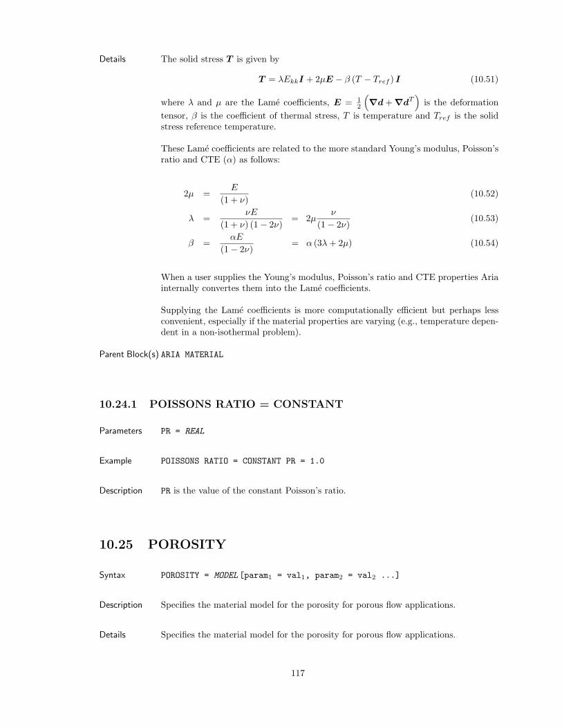
Details The solid stress T is given by
T = λEkkI + 2µE − β (T − Tref ) I (10.51)
where λ and µ are the Lame coefficients, E = 12
(∇d + ∇dT
)is the deformation
tensor, β is the coefficient of thermal stress, T is temperature and Tref is the solidstress reference temperature.
These Lame coefficients are related to the more standard Young’s modulus, Poisson’sratio and CTE (α) as follows:
2µ =E
(1 + ν)(10.52)
λ =νE
(1 + ν) (1− 2ν)= 2µ
ν
(1− 2ν)(10.53)
β =αE
(1− 2ν)= α (3λ + 2µ) (10.54)
When a user supplies the Young’s modulus, Poisson’s ratio and CTE properties Ariainternally convertes them into the Lame coefficients.
Supplying the Lame coefficients is more computationally efficient but perhaps lessconvenient, especially if the material properties are varying (e.g., temperature depen-dent in a non-isothermal problem).
Parent Block(s) ARIA MATERIAL
10.24.1 POISSONS RATIO = CONSTANT
Parameters PR = REAL
Example POISSONS RATIO = CONSTANT PR = 1.0
Description PR is the value of the constant Poisson’s ratio.
10.25 POROSITY
Syntax POROSITY = MODEL [param1 = val1, param2 = val2 ...]
Description Specifies the material model for the porosity for porous flow applications.
Details Specifies the material model for the porosity for porous flow applications.
117
Parent Block(s) ARIA MATERIAL
10.25.1 POROSITY = CONSTANT
Parameters PHI = REAL
Example Porosity = Constant PHI=0.1
Description The value is constant in space and time.
10.25.2 POROSITY = POLYNOMIAL
Parameters VARIABLE = STRING
ORDER = INT
[C0 = REAL ][C1 = REAL ]...[CN = REAL ]
Example Porosity = Polynomial Variable=Coordinates X Order=1 C0=0.1 C1=0.01
Description Arbitrary order polynomial function of a specified scalar variable.
φ =N∑
i=0
CiXi (10.55)
Here, N is the order of the polynomial provided by the ORDER parameter and X isthe variable supplied by the VARIABLE parameter and Ci are the supplied coefficients.Coefficients that are not supplied default to a value of zero. The VARIABLE argumentcan be TIME or any internal Expression that evaluates to a scalar. For the latter case,the format of the VARIABLE argument is described in section 2.6.1.
10.26 RELATIVE PERMEABILITY
Syntax RELATIVE PERMEABILITY = MODEL [param1 = val1, param2 = val2 ...]
Description Specifies the material model for the relative permeability (scalar) for porous flow inDarcy’s Law.
118
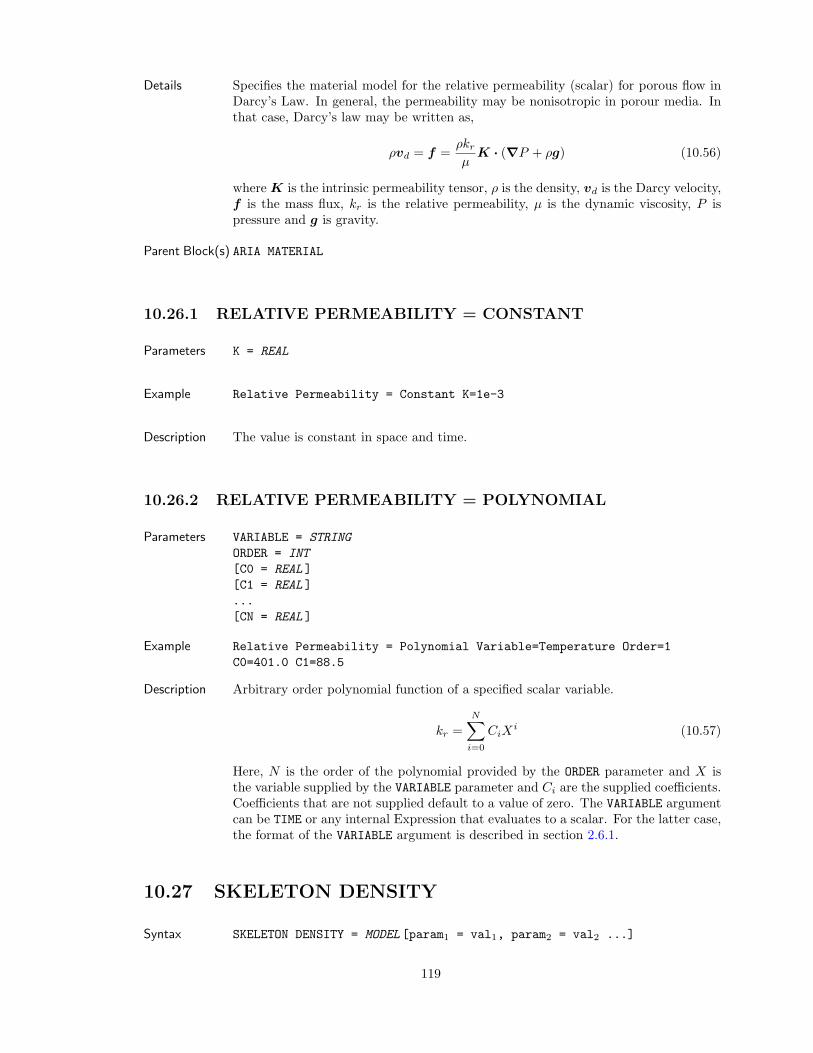
Details Specifies the material model for the relative permeability (scalar) for porous flow inDarcy’s Law. In general, the permeability may be nonisotropic in porour media. Inthat case, Darcy’s law may be written as,
ρvd = f =ρkr
µK · (∇P + ρg) (10.56)
where K is the intrinsic permeability tensor, ρ is the density, vd is the Darcy velocity,f is the mass flux, kr is the relative permeability, µ is the dynamic viscosity, P ispressure and g is gravity.
Parent Block(s) ARIA MATERIAL
10.26.1 RELATIVE PERMEABILITY = CONSTANT
Parameters K = REAL
Example Relative Permeability = Constant K=1e-3
Description The value is constant in space and time.
10.26.2 RELATIVE PERMEABILITY = POLYNOMIAL
Parameters VARIABLE = STRING
ORDER = INT
[C0 = REAL ][C1 = REAL ]...[CN = REAL ]
Example Relative Permeability = Polynomial Variable=Temperature Order=1C0=401.0 C1=88.5
Description Arbitrary order polynomial function of a specified scalar variable.
kr =N∑
i=0
CiXi (10.57)
Here, N is the order of the polynomial provided by the ORDER parameter and X isthe variable supplied by the VARIABLE parameter and Ci are the supplied coefficients.Coefficients that are not supplied default to a value of zero. The VARIABLE argumentcan be TIME or any internal Expression that evaluates to a scalar. For the latter case,the format of the VARIABLE argument is described in section 2.6.1.
10.27 SKELETON DENSITY
Syntax SKELETON DENSITY = MODEL [param1 = val1, param2 = val2 ...]
119
Description Specifies a model for the porous skeleton density of a material.
Details Specifies a model for the porous skeleton density of a material.
Parent Block(s) ARIA MATERIAL
10.27.1 SKELETON DENSITY = CONSTANT
Parameters RHO = REAL
Example Skeleton Density = Constant Rho=1e3
Description The value is constant in space and time.
10.28 SKELETON INTERNAL ENERGY
Syntax SKELETON INTERNAL ENERGY = MODEL [param1 = val1, param2 = val2 ...]
Description Specifies a model for the porous skeleton internal energy of a material.
Details Specifies a model for the porous skeleton internal energy of a material.
Parent Block(s) ARIA MATERIAL
10.28.1 SKELETON INTERNAL ENERGY = CONSTANT
Parameters E = REAL
Example Skeleton Internal Energy = Constant E=2.3e-4
Description The value is constant in space and time.
10.28.2 SKELETON INTERNAL ENERGY = LINEAR
Parameters CP = REAL
T REF = REAL
120
Example Skeleton Internal Energy = Linear Cp=13.7 T ref=298.15
Description The internel energy of the porous skeleton, es, is given by the simple relation,
es = Cp (T − Tref ) (10.58)
where Cp is the specific heat supplied by the CP parameter and Tref is a referencetemperature supplied by the T REF parameter. This model also supplies the timederivative of es,
∂es
∂t= Cp
∂T
∂t(10.59)
10.29 SOLID STRESS
Syntax SOLID STRESS = MODEL [param1 = val1, param2 = val2 ...]
Description Specifies a contribution to the solid stress tensor. Multiple stresses are combinedadditvely and may be specified by using this line command multiple times.
Details Specifies a contribution to the solid stress tensor. The total stress T is given by
T =∑
j
T j (10.60)
Parent Block(s) ARIA MATERIAL
10.29.1 SOLID STRESS = ISOTHERMAL
Parameters T = REAL
T REF = REAL
Example SOLID STRESS = Isothermal T=500 T ref=325
Description This stress accounts for the mechanical stresses due to thermally induced strains.
T = −β (T − Tref ) I (10.61)
where β is the Lame coefficient of thermal stress (related to the coefficient of thermalexpansion, α), T is the temperature and Tref is the temperature of the undeformedreference state of the mesh (pseudo-solid). This is a specialization of the THERMALmodel that uses uniform, fixed temperature and reference temperature.
10.29.2 SOLID STRESS = LINEAR ELASTIC
Parameters REFERENCE FRAME = ‘‘MOVING’’ | ‘‘UNDEFORMED’’
121
Example SOLID STRESS = Linear Elastic Reference Frame=Moving
Description Supplies the linear elasticity stress tensor,
T = λ trace EI + 2µE (10.62)
where λ and µ and the Lame coefficients and E is the strain tensor. When thechoice of refernce frame is “UNDEFORMED” then the strain is computed in theundeformed reference state; this is commonly referred to as small strain theory. Whenthe reference frame is “MOVING” then the strain is computed with respect to thedeformed coordinates.
Specifically, the strain tensor is given by
E =12(∇d + ∇dt
)(10.63)
where d is the solid displacement field. The choice of reference frame determineswhether the ∇ operator is computed in the undeformed or moving reference frames.
10.29.3 SOLID STRESS = NEOHOOKEAN ELASTIC
Parameters (none)
Example SOLID STRESS = Neohookean Elastic
Description Supplies a nonlinear hyperelastic stress of the form,
T =µ
J(b− I) +
λ
JlnJI (10.64)
where λ and µ and the Lame coefficients, b ≡ F ·F t is the left Cauchy-Green tensor,F is the deformation gradient and J ≡ det F . See, e.g., Bonet and Wood (1997) orBelytschko et al. (2004).
10.29.4 SOLID STRESS = NONLINEAR ELASTIC
Parameters (none)
Example SOLID STRESS = Nonlinear Elastic
122
Description Supplies a nonlinear elastic stress,
T = λ trace EI + 2µE (10.65)
where λ and µ and the Lame coefficients and E is the strain tensor. The particularchoice of strain tensor chosen depends on where the configuration (reference frame)which is set via the MESH MOTION command line. See section 3.11 for moreinformation. When the MESH MOTION is set to ARBITRARY then the Greenstrain is used. Otherwise, the Almansi strain is used.
10.29.5 SOLID STRESS = RESIDUAL
Parameters [SXX | SX = REAL ][SYY | SY = REAL ][SZZ | SZ = REAL ][SXY = REAL ][SXZ = REAL ][SYZ = REAL ]
Example SOLID STRESS = Residual Sxx=0.02 Syy=0.02
Description This stress accounts for the initial residual stress in a solid that is constant anduniform everywhere. The components of the residual stress tensor are supplied bythe (up-to) six components SXX, SYY, SZZ, SXY, SXZ, and SYZ.
This is directly analogous to the ISTRESS condition in ANSYS. To that end, thediagonal components can be specified as either SXX or SX etc.
10.29.6 SOLID STRESS = THERMAL
Parameters (none)
Example SOLID STRESS = Thermal
Description This stress accounts for the mechanical stresses due to thermally induced strains.
T = −β (T − Tref ) I (10.66)
where β is the Lame coefficient of thermal stress (related to the coefficient of thermalexpansion, α), T is the temperature and Tref is the temperature of the undeformedreference state of the solid.
10.30 SPECIES DIFFUSION
Syntax SPECIES DIFFUSION = MODEL [param1 = val1, param2 = val2 ...]
123
Description Specifies the material (constitutive) model for the species diffusion (diffusive flux) inthe bulk.
Details Specifies the material (constitutive) model for the species diffusion (diffusive flux) inthe bulk.
Parent Block(s) ARIA MATERIAL
10.30.1 SPECIES DIFFUSION = BASIC
This is an alias for FICKS LAW.
Example Species Diffusion = Basic
10.30.2 SPECIES DIFFUSION = FICKS LAW
Parameters (none)
Example Species Diffusion = Ficks Law
Description The diffusive species flux q is given by Fick’s Law,
q = −D∇C (10.67)
where D is the species diffusivity and C is the species concentration.
10.31 SPECIES DIFFUSIVITY
Syntax SPECIES DIFFUSIVITY = MODEL [param1 = val1, param2 = val2 ...]
Description Specifies the material model for the species diffusivity.
Details Specifies the material model for the species diffusivity.
Parent Block(s) ARIA MATERIAL
10.31.1 SPECIES DIFFUSIVITY = CONSTANT
Parameters D = REAL
Example SPECIES DIFFUSIVITY = CONSTANT D = 1.0
124
Description D is the value of the constant species diffusivity.
10.32 SPECIFIC HEAT
Syntax SPECIFIC HEAT = MODEL [param1 = val1, param2 = val2 ...]
Description Specifies the material model for the specific heat.
Details Specifies the material model for the specific heat.
Parent Block(s) ARIA MATERIAL
10.32.1 SPECIFIC HEAT = CONSTANT
Parameters CP = REAL
Example SPECIFIC HEAT = CONSTANT CP = 1.0
Description CP is the value of the constant specific heat.
10.32.2 SPECIFIC HEAT = CURING FOAM
Parameters VFRAC SUBINDEX = INT
[CP FL = REAL ][CP FG = REAL ][CP E = REAL ][PHI ZERO = REAL ]
Example Specific Heat = Curing Foam Vfrac Subindex=1 Cp fL=1 Cp fG=1 Cp e=1phi zero=0.2
125

Description For a curing expoxy with volume fraction φ the specific heat is given by
Cp = Cp,fLφ + Cp,fG
(φ − φ) + Cp,e (1− φ) (10.68)= a + bφ (10.69)
where Cp,fLis the specific heat of the liquid phase flourinert, Cp,fG
is the specificheat of the gas phase flourinert, Cp,e is the specific heat of the epoxy and φ is thereference volume fraction in the flourinert. In the latter form of this relationship
a = Cp,fL− Cp,fG
(10.70)b = Cp,fG
φ + Cp,e(1− φ). (10.71)
NOTE: The volume fraction is assumed to be a SPECIES field with the subindexprovided by the VFRAC SUBINDEX parameter.
10.32.3 SPECIFIC HEAT = EXPONENTIAL
Parameters VARIABLE = STRING
[CONSTANT = REAL ][MULTIPLIER = REAL ]EXPONENT = REAL
Example Specific Heat = Exponential Variable=Temperature Multiplier=1.0Exponent=-0.3
Description Exponential function of in specified scalar variable. The specific heat is computed as
Cp = C + MeEX (10.72)
Here, C is the constant term supplied by the CONSTANT parameter which defaults tozero, M is the value supplied by the MULTIPLIER parameter which defaults to unity,X is the variable supplied by the VARIABLE parameter and E is the exponentialmultiplier provided by the EXPONENT parameter.
10.32.4 SPECIFIC HEAT = POLYNOMIAL
Parameters VARIABLE = STRING
ORDER = INT
[C0 = REAL ][C1 = REAL ]...[CN = REAL ]
Example Specific Heat = Polynomial Variable=Temperature Order=1 C0=401.0C1=88.5
126
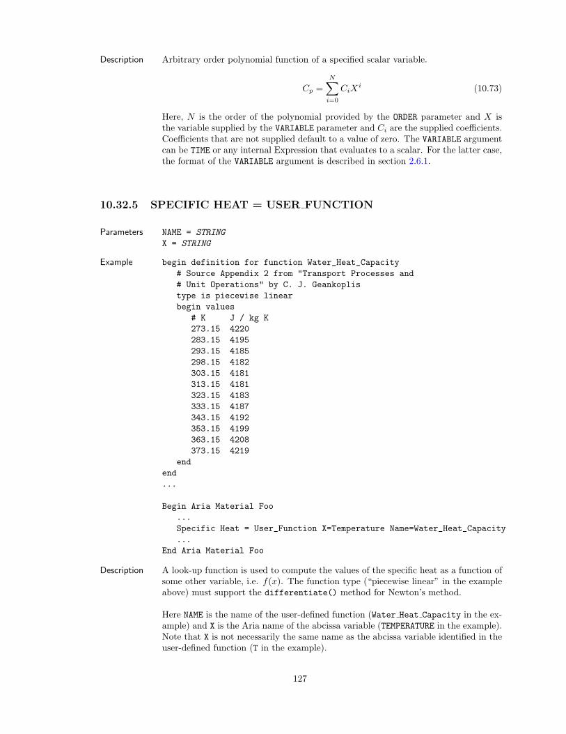
Description Arbitrary order polynomial function of a specified scalar variable.
Cp =N∑
i=0
CiXi (10.73)
Here, N is the order of the polynomial provided by the ORDER parameter and X isthe variable supplied by the VARIABLE parameter and Ci are the supplied coefficients.Coefficients that are not supplied default to a value of zero. The VARIABLE argumentcan be TIME or any internal Expression that evaluates to a scalar. For the latter case,the format of the VARIABLE argument is described in section 2.6.1.
10.32.5 SPECIFIC HEAT = USER FUNCTION
Parameters NAME = STRING
X = STRING
Example begin definition for function Water_Heat_Capacity# Source Appendix 2 from "Transport Processes and# Unit Operations" by C. J. Geankoplistype is piecewise linearbegin values
# K J / kg K273.15 4220283.15 4195293.15 4185298.15 4182303.15 4181313.15 4181323.15 4183333.15 4187343.15 4192353.15 4199363.15 4208373.15 4219
endend...
Begin Aria Material Foo...Specific Heat = User_Function X=Temperature Name=Water_Heat_Capacity...
End Aria Material Foo
Description A look-up function is used to compute the values of the specific heat as a function ofsome other variable, i.e. f(x). The function type (“piecewise linear” in the exampleabove) must support the differentiate() method for Newton’s method.
Here NAME is the name of the user-defined function (Water Heat Capacity in the ex-ample) and X is the Aria name of the abcissa variable (TEMPERATURE in the example).Note that X is not necessarily the same name as the abcissa variable identified in theuser-defined function (T in the example).
127
10.33 SURFACE TENSION
Syntax SURFACE TENSION = MODEL [param1 = val1, param2 = val2 ...]
Description Specifies the model to use for the surface (interfacial) tension.
Details Specifies the model to use for the surface (interfacial) tension.
Parent Block(s) ARIA MATERIAL
10.33.1 SURFACE TENSION = CONSTANT
Parameters SIGMA = REAL
Example Surface Tension = Constant Sigma = 72.0
Description SIGMA is the value of the surface tension.
10.33.2 SURFACE TENSION = LINEAR T
Parameters SIGMA0 = REAL
DSIGMADT = REAL
T REF = REAL
Example Surface Tension = Linear T sigma0=72. dsigmadT = -.15 T ref =298.
Description SIGMA0 is the value of the surface tension at the reference temperature T REF andDSIGMADT is the derivative of the surface temperature with respect to temperature,i.e.,
σ = σ0 + m(T − Tref ) (10.74)
where m is DSIGMADT.
10.34 SUSPENSION FLUX
Syntax SUSPENSION FLUX = MODEL [param1 = val1, param2 = val2 ...]
Description Specifies the parameters for the suspension flux model.
Details Specifies the suspension flux model and its parameters for this material.
128
Parent Block(s) ARIA MATERIAL
10.34.1 SUSPENSION FLUX = PHILLIPS
Parameters K mu = REAL
K c = REAL
phi max = REAL
beta = REAL
particle radius = REAL
Example SUSPENSION FLUX = Phillips K mu=0.62 K c=0.41 phi max=0.68 beta=-1.82particle radius=0.01
Description The Phillips diffusive flux model is intended to be used in conjunction with the Kriegerviscosity model (10.40.8). Here, the flux is given by
q =(
Kca2 −Kµa2β
φ
φm − φ
)γφ∇φ + Kca
2φ2∇γ (10.75)
where γ is the shear rate, φ is the suspension concentration, φm is the maximumsuspension concentration and a is the particle radius.
10.35 THERMAL CONDUCTIVITY
Syntax THERMAL CONDUCTIVITY = MODEL [param1 = val1, param2 = val2 ...]
Description Specifies the material model for the thermal conductivity.
Details Specifies the material model for the thermal conductivity that appears in the diffusionterm of the energy equation for temperature.
Parent Block(s) ARIA MATERIAL
10.35.1 THERMAL CONDUCTIVITY = CONSTANT
Parameters K = REAL
Example THERMAL CONDUCTIVITY = CONSTANT K = 1.0
Description K is the value of the constant thermal conductivity.
129
10.35.2 THERMAL CONDUCTIVITY = CURING FOAM
Parameters RHO E = REAL
K F = REAL
K E = REAL
Example Thermal Conductivity = Curing Foam rho e=1.3 k e=14 k f=2.7
Description For a curing expoxy with mixture density ρ
κ =23
(ρ
ρe
)κe +
(1− ρ
ρe
)κf (10.76)
= a + bρ (10.77)
where ρe is the density of the expoxy, κe is the thermal conductivity of the epoxy andκf is the thermal conductivity of the fourinert. In the latter form of this relationship
a = κf (10.78)
b =1ρe
(23κe − κf
)(10.79)
10.35.3 THERMAL CONDUCTIVITY = POLYNOMIAL
Parameters VARIABLE = STRING
ORDER = INT
[C0 = REAL ][C1 = REAL ]...[CN = REAL ]
Example Thermal Conductivity = Polynomial Variable=Temperature Order=1C0=401.0 C1=88.5
Description Arbitrary order polynomial function of a specified scalar variable.
κ =N∑
i=0
CiXi (10.80)
Here, N is the order of the polynomial provided by the ORDER parameter and X isthe variable supplied by the VARIABLE parameter and Ci are the supplied coefficients.Coefficients that are not supplied default to a value of zero. The VARIABLE argumentcan be TIME or any internal Expression that evaluates to a scalar. For the latter case,the format of the VARIABLE argument is described in section 2.6.1.
130
10.35.4 THERMAL CONDUCTIVITY = THERMAL
Parameters [A = REAL ][B = REAL ][C = REAL ][D = REAL ]
Example THERMAL CONDUCTIVITY = THERMAL A = 401.0 B = 88.5
Description Cubic polynomial function of temperature for the conductivity.
κ = A + BT + CT 2 + DT 3 (10.81)
10.35.5 THERMAL CONDUCTIVITY = USER FUNCTION
Parameters NAME = STRING
X = STRING
Example begin definition for function SI_Ktype is piecewise linearbegin values
20.0 5.50e7100.0 4.60e7...800.0 1.30e7
2000.0 1.30e7end values
end definition for function SI_K
...
Begin Aria Material Foo...Thermal Conductivity = User_Function Name=SI_K X=Temperature...
End Aria Material Foo
Description A look-up function is used to compute the values of the thermal conductivity as afunction of some other variable, i.e. f(x). The function type (“piecewise linear” in theexample above) must support the differentiate() method for Newton’s method.
Here NAME is the name of the user-defined function (RESISTANCE DATA in the example)and X is the Aria name of the abcissa variable (TEMPERATURE in the example). Notethat X is not necessarily the same name as the optional abcissa variable identified inthe user-defined function.
131
10.36 THERMAL DIFFUSIVITY
Syntax THERMAL DIFFUSIVITY = MODEL [param1 = val1, param2 = val2 ...]
Description Specifies the material model for the thermal diffusivity.
Details Specifies the material model for the thermal diffusivity.
Parent Block(s) ARIA MATERIAL
10.36.1 THERMAL DIFFUSIVITY = CONSTANT
Parameters D = REAL
Example THERMAL DIFFUSIVITY = CONSTANT D = 1.0
Description D is the value of the constant thermal diffusivity.
10.37 TOTAL INTERNAL ENERGY
Syntax TOTAL INTERNAL ENERGY = MODEL [param1 = val1, param2 = val2 ...]
Description Specifies a model for the total internal energy of a material.
Details Specifies a model for the total internal of a material.
Parent Block(s) ARIA MATERIAL
10.37.1 TOTAL INTERNAL ENERGY = POROUS
Parameters (none)
Example Total Internal Energy = Porous
132
Description The total internal energy e is computed as
e = (1− φ)ρses + φ ∗ ρfef (10.82)
where φ is the porosity, ρs is the density of the solid porous skeleton, es is the internalenergy of the solid porous skeleton, ρf is the density of the fluid phase and ef is theinternal energy of the fluid phase.
10.38 TWO MU
Syntax TWO MU = MODEL [param1 = val1, param2 = val2 ...]
Description Specifies the material model for twice the µ Lame coefficient.
Details The solid stress T is given by
T = λEkkI + 2µE − β (T − Tref ) I (10.83)
where λ and µ are the Lame coefficients, E = 12
(∇d + ∇dT
)is the deformation
tensor, β is the coefficient of thermal stress, T is temperature and Tref is the solidstress reference temperature.
These Lame coefficients are related to the more standard Young’s modulus, Poisson’sratio and CTE (α) as follows:
2µ =E
(1 + ν)(10.84)
λ =νE
(1 + ν) (1− 2ν)= 2µ
ν
(1− 2ν)(10.85)
β =αE
(1− 2ν)= α (3λ + 2µ) (10.86)
When a user supplies the Young’s modulus, Poisson’s ratio and CTE properties Ariainternally convertes them into the Lame coefficients.
Parent Block(s) ARIA MATERIAL
10.38.1 TWO MU = CONSTANT
Parameters TWO MU = REAL
Example TWO MU = CONSTANT TWO MU = 1.0
Description TWO MU is the value of 2µ.
133
10.38.2 TWO MU = CONVERTED
Parameters (None)
Example TWO MU = Converted
Description Aria will use Young’s modulus and Poisson ratio to compute the Lame µ coefficient.Supplying the Lame coefficients is more computationally efficient but perhaps lessconvenient, especially if the material properties are varying (e.g., temperature depen-dent in a non-isothermal problem).
10.39 VALENCE
Syntax VALENCE = MODEL [param1 = val1, param2 = val2 ...]
Description Specifies the valence (net charge) for a species.
Details Specifies the valence (net charge) for a species.
Parent Block(s) ARIA MATERIAL
10.39.1 VALENCE = CONSTANT
Parameters Z = REAL
[SUBINDEX = INT ]
Example Valence = Constant Subindex=1 Z = 1Valence = Constant Subindex=2 Z = -1Valence = Constant Subindex=5 Z = -2
Description Z is the value of the species valence.
SUBINDEX is the species subindex.
10.40 VISCOSITY
Syntax VISCOSITY = MODEL [param1 = val1, param2 = val2 ...]
Description Specifies the material model for the fluid viscosity.
Details Specifies the material model for the fluid viscosity.
134
Parent Block(s) ARIA MATERIAL
10.40.1 VISCOSITY = ARRHENIUS
Parameters mu0 = REAL
E = REAL
Example VISCOSITY = Arrhenius mu0=16.4 E=5000.
Description This model provides a viscosity with an Arrhenius temperature dependence:
µ = µ0e−E/T (10.87)
where T is the temperature.
10.40.2 VISCOSITY = BINGHAM WLF
Parameters MU ZERO = REAL
MU INF = REAL
F = REAL
N = REAL
A = REAL
LAMBDA = REAL
TAU Y = REAL
Example VISCOSITY = Bingham WLF ...
Description
µ = µ∞ +(
µ − µ∞ + τy1− e−γF
γ
)(1 + (λγ)a)
n−1a (10.88)
where γ is the shear rate.
10.40.3 VISCOSITY = BINGHAM WLFT
Parameters MU ZERO = REAL
MU INF = REAL
F = REAL
N = REAL
A = REAL
LAMBDA = REAL
TAU Y = REAL
C 1 = REAL
C 2 = REAL
T REF = REAL
Example VISCOSITY = Bingham WLFT ...
135
Description
µ = aT
(µ∞ +
(µ − µ∞ + τy
1− e−aT γF
aT γ
)(1 + (aT λγ)a)
n−1a
)(10.89)
whereaT = e
c1(T−T )c2+T−T (10.90)
and T is the temperature and γ is the shear rate.
10.40.4 VISCOSITY = CARREAU
Parameters MU ZERO = REAL
[MU INF = REAL ][A = REAL ]N = REAL
LAMBDA = REAL
Example Viscosity = Carreau ...
Descriptionµ− µ∞µ − µ∞
= (1 + (λγ)a)n−1
a (10.91)
orµ = µ∞ + (µ − µ∞) (1 + (λγ)a)
n−1a (10.92)
where µ∞ is the infinite shear viscosity (MU INF, defaults to zero), µ is the zero shearviscosity (MU ZERO), n (N) and a (A, defaults to 2) are model parameters, γ is the shearrate and λ (LAMBDA) is a time constant.
10.40.5 VISCOSITY = CARREAU T
Parameters MU ZERO = REAL
[MU INF = REAL ][A = REAL ]N = REAL
K = REAL
Example Viscosity = Carreau T ...
Descriptionµ− µ∞µ − µ∞
=(1 +
(ek/T γ
)a)n−1a
(10.93)
or
µ = µ∞ + (µ − µ∞)(1 +
(ek/T γ
)a)n−1a
(10.94)
where µ∞ is the infinite shear viscosity (MU INF, defaults to zero), µ is the zeroshear viscosity (MU ZERO), n (N) and a (A, defaults to 2) are model parameters and γis the shear rate. The quantity ek/T , where T is temperature and k (K) is a referencetemperature, is a temperature dependent time scale; it takes the place of the constantλ time scale in the CARREAU model.
136
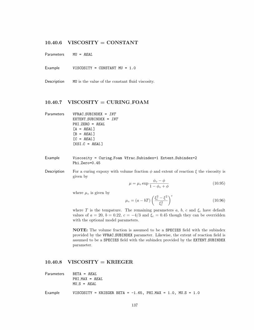
10.40.6 VISCOSITY = CONSTANT
Parameters MU = REAL
Example VISCOSITY = CONSTANT MU = 1.0
Description MU is the value of the constant fluid viscosity.
10.40.7 VISCOSITY = CURING FOAM
Parameters VFRAC SUBINDEX = INT
EXTENT SUBINDEX = INT
PHI ZERO = REAL
[A = REAL ][B = REAL ][C = REAL ][KSI C = REAL ]
Example Viscosity = Curing Foam Vfrac Subindex=1 Extent Subindex=2Phi Zero=0.45
Description For a curing expoxy with volume fraction φ and extent of reaction ξ the viscosity isgiven by
µ = µ expφ − φ
1− φ + φ(10.95)
where µ is given by
µ = (a− bT )(
ξ2c − ξ2
ξ2c
)c
(10.96)
where T is the tempature. The remaining parameters a, b, c and ξc have defaultvalues of a = 20, b = 0.22, c = −4/3 and ξc = 0.45 though they can be overriddenwith the optional model parameters.
NOTE: The volume fraction is assumed to be a SPECIES field with the subindexprovided by the VFRAC SUBINDEX parameter. Likewise, the extent of reaction field isassumed to be a SPECIES field with the subindex provided by the EXTENT SUBINDEXparameter.
10.40.8 VISCOSITY = KRIEGER
Parameters BETA = REAL
PHI MAX = REAL
MU S = REAL
Example VISCOSITY = KRIEGER BETA = -1.65, PHI MAX = 1.0, MU S = 1.0
137
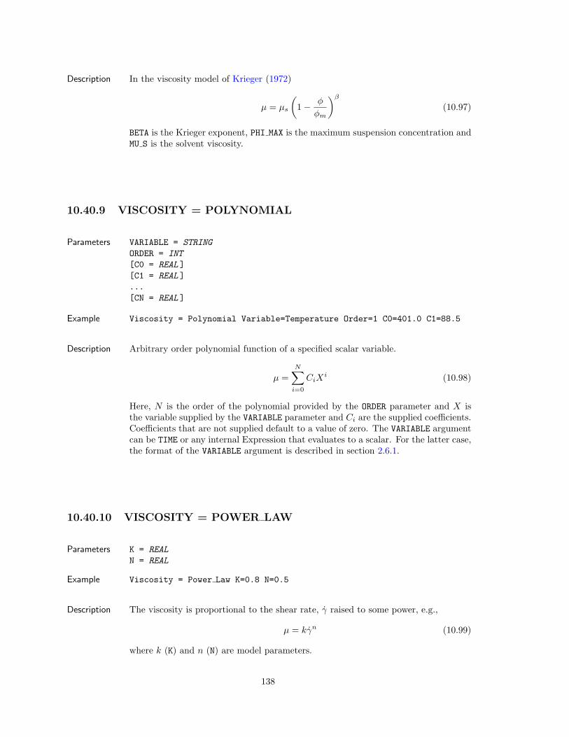
Description In the viscosity model of Krieger (1972)
µ = µs
(1− φ
φm
)β
(10.97)
BETA is the Krieger exponent, PHI MAX is the maximum suspension concentration andMU S is the solvent viscosity.
10.40.9 VISCOSITY = POLYNOMIAL
Parameters VARIABLE = STRING
ORDER = INT
[C0 = REAL ][C1 = REAL ]...[CN = REAL ]
Example Viscosity = Polynomial Variable=Temperature Order=1 C0=401.0 C1=88.5
Description Arbitrary order polynomial function of a specified scalar variable.
µ =N∑
i=0
CiXi (10.98)
Here, N is the order of the polynomial provided by the ORDER parameter and X isthe variable supplied by the VARIABLE parameter and Ci are the supplied coefficients.Coefficients that are not supplied default to a value of zero. The VARIABLE argumentcan be TIME or any internal Expression that evaluates to a scalar. For the latter case,the format of the VARIABLE argument is described in section 2.6.1.
10.40.10 VISCOSITY = POWER LAW
Parameters K = REAL
N = REAL
Example Viscosity = Power Law K=0.8 N=0.5
Description The viscosity is proportional to the shear rate, γ raised to some power, e.g.,
µ = kγn (10.99)
where k (K) and n (N) are model parameters.
138
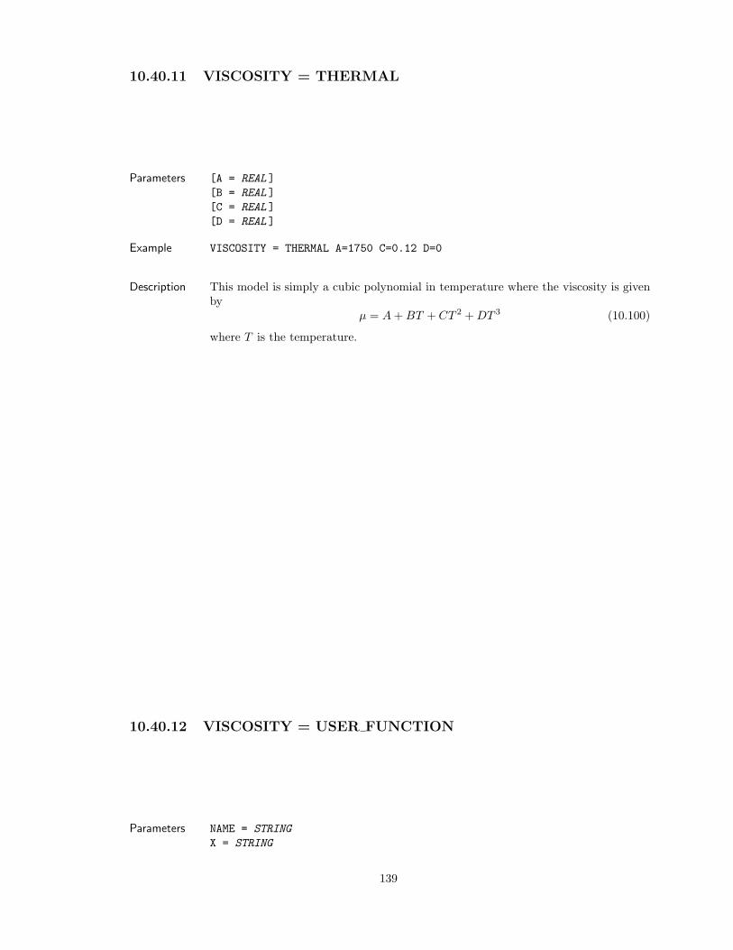
10.40.11 VISCOSITY = THERMAL
Parameters [A = REAL ][B = REAL ][C = REAL ][D = REAL ]
Example VISCOSITY = THERMAL A=1750 C=0.12 D=0
Description This model is simply a cubic polynomial in temperature where the viscosity is givenby
µ = A + BT + CT 2 + DT 3 (10.100)
where T is the temperature.
10.40.12 VISCOSITY = USER FUNCTION
Parameters NAME = STRING
X = STRING
139
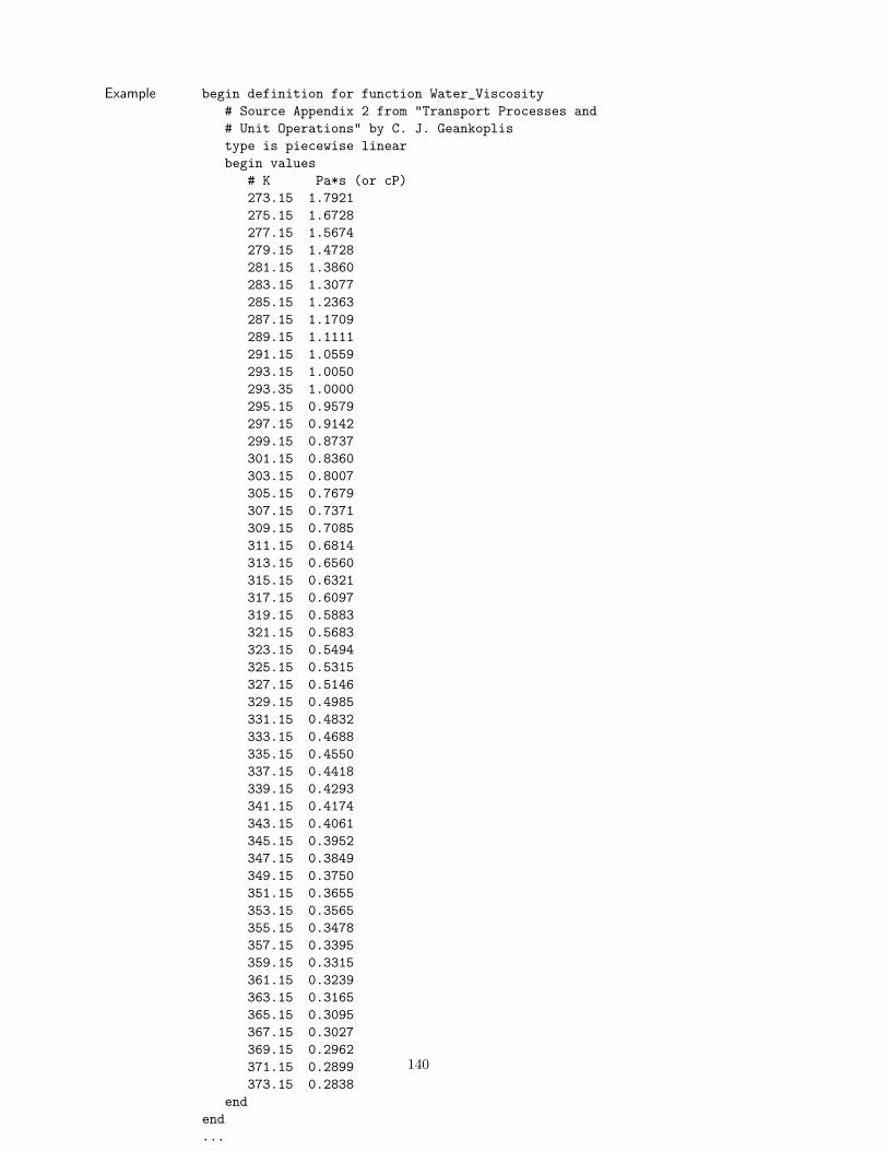
Example begin definition for function Water_Viscosity# Source Appendix 2 from "Transport Processes and# Unit Operations" by C. J. Geankoplistype is piecewise linearbegin values
# K Pa*s (or cP)273.15 1.7921275.15 1.6728277.15 1.5674279.15 1.4728281.15 1.3860283.15 1.3077285.15 1.2363287.15 1.1709289.15 1.1111291.15 1.0559293.15 1.0050293.35 1.0000295.15 0.9579297.15 0.9142299.15 0.8737301.15 0.8360303.15 0.8007305.15 0.7679307.15 0.7371309.15 0.7085311.15 0.6814313.15 0.6560315.15 0.6321317.15 0.6097319.15 0.5883321.15 0.5683323.15 0.5494325.15 0.5315327.15 0.5146329.15 0.4985331.15 0.4832333.15 0.4688335.15 0.4550337.15 0.4418339.15 0.4293341.15 0.4174343.15 0.4061345.15 0.3952347.15 0.3849349.15 0.3750351.15 0.3655353.15 0.3565355.15 0.3478357.15 0.3395359.15 0.3315361.15 0.3239363.15 0.3165365.15 0.3095367.15 0.3027369.15 0.2962371.15 0.2899373.15 0.2838
endend...
Begin Aria Material Foo...Viscosity = User_Function Name=Water_Viscosity X=Temperature...
End Aria Material Foo
140
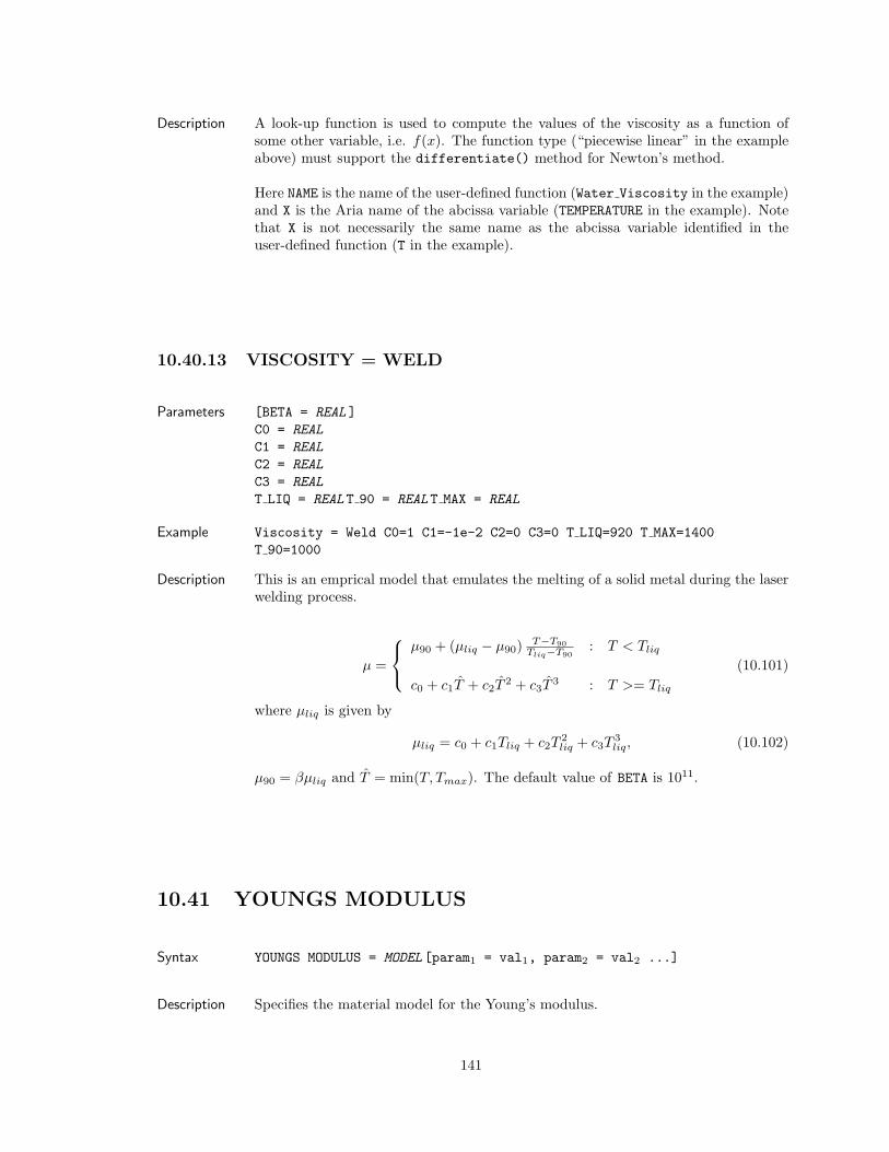
Description A look-up function is used to compute the values of the viscosity as a function ofsome other variable, i.e. f(x). The function type (“piecewise linear” in the exampleabove) must support the differentiate() method for Newton’s method.
Here NAME is the name of the user-defined function (Water Viscosity in the example)and X is the Aria name of the abcissa variable (TEMPERATURE in the example). Notethat X is not necessarily the same name as the abcissa variable identified in theuser-defined function (T in the example).
10.40.13 VISCOSITY = WELD
Parameters [BETA = REAL ]C0 = REAL
C1 = REAL
C2 = REAL
C3 = REAL
T LIQ = REAL T 90 = REAL T MAX = REAL
Example Viscosity = Weld C0=1 C1=-1e-2 C2=0 C3=0 T LIQ=920 T MAX=1400T 90=1000
Description This is an emprical model that emulates the melting of a solid metal during the laserwelding process.
µ =
µ90 + (µliq − µ90) T−T90
Tliq−T90: T < Tliq
c0 + c1T + c2T2 + c3T
3 : T >= Tliq
(10.101)
where µliq is given by
µliq = c0 + c1Tliq + c2T2liq + c3T
3liq, (10.102)
µ90 = βµliq and T = min(T, Tmax). The default value of BETA is 1011.
10.41 YOUNGS MODULUS
Syntax YOUNGS MODULUS = MODEL [param1 = val1, param2 = val2 ...]
Description Specifies the material model for the Young’s modulus.
141
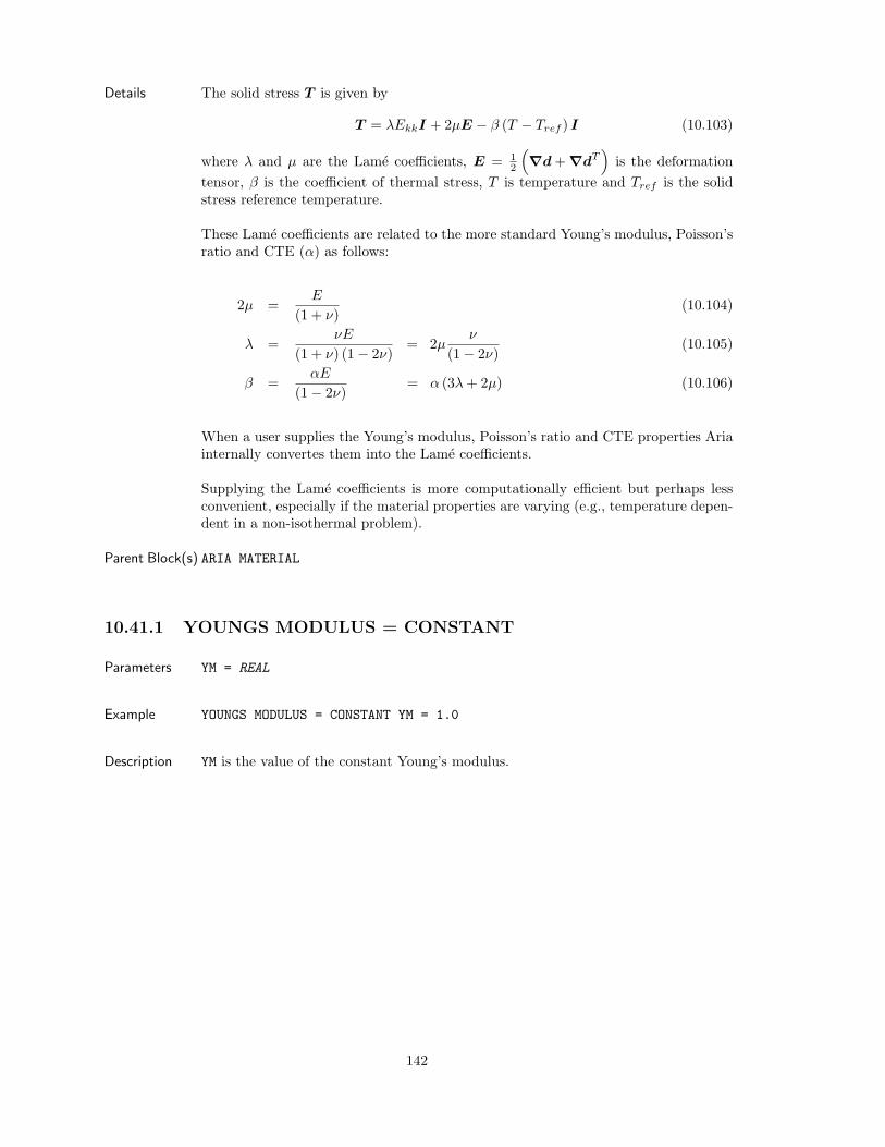
Details The solid stress T is given by
T = λEkkI + 2µE − β (T − Tref ) I (10.103)
where λ and µ are the Lame coefficients, E = 12
(∇d + ∇dT
)is the deformation
tensor, β is the coefficient of thermal stress, T is temperature and Tref is the solidstress reference temperature.
These Lame coefficients are related to the more standard Young’s modulus, Poisson’sratio and CTE (α) as follows:
2µ =E
(1 + ν)(10.104)
λ =νE
(1 + ν) (1− 2ν)= 2µ
ν
(1− 2ν)(10.105)
β =αE
(1− 2ν)= α (3λ + 2µ) (10.106)
When a user supplies the Young’s modulus, Poisson’s ratio and CTE properties Ariainternally convertes them into the Lame coefficients.
Supplying the Lame coefficients is more computationally efficient but perhaps lessconvenient, especially if the material properties are varying (e.g., temperature depen-dent in a non-isothermal problem).
Parent Block(s) ARIA MATERIAL
10.41.1 YOUNGS MODULUS = CONSTANT
Parameters YM = REAL
Example YOUNGS MODULUS = CONSTANT YM = 1.0
Description YM is the value of the constant Young’s modulus.
142
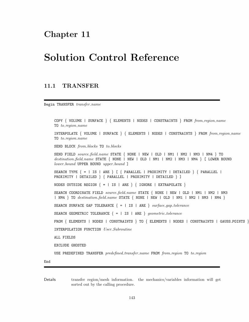
Chapter 11
Solution Control Reference
11.1 TRANSFER
Begin TRANSFER transfer name
COPY VOLUME | SURFACE ELEMENTS | NODES | CONSTRAINTS FROM from region nameTO to region name
INTERPOLATE VOLUME | SURFACE ELEMENTS | NODES | CONSTRAINTS FROM from region nameTO to region name
SEND BLOCK from blocks TO to blocks
SEND FIELD source field name STATE NONE | NEW | OLD | NM1 | NM2 | NM3 | NM4 TOdestination field name STATE NONE | NEW | OLD | NM1 | NM2 | NM3 | NM4 [ LOWER BOUNDlower bound UPPER BOUND upper bound ]
SEARCH TYPE = | IS | ARE [ PARALLEL | PROXIMITY | DETAILED PARALLEL |PROXIMITY | DETAILED PARALLEL | PROXIMITY | DETAILED ]
NODES OUTSIDE REGION = | IS | ARE IGNORE | EXTRAPOLATE
SEARCH COORDINATE FIELD source field name STATE NONE | NEW | OLD | NM1 | NM2 | NM3| NM4 TO destination field name STATE NONE | NEW | OLD | NM1 | NM2 | NM3 | NM4
SEARCH SURFACE GAP TOLERANCE = | IS | ARE surface gap tolerance
SEARCH GEOMETRIC TOLERANCE = | IS | ARE geometric tolerance
FROM ELEMENTS | NODES | CONSTRAINTS TO ELEMENTS | NODES | CONSTRAINTS | GAUSS POINTS
INTERPOLATION FUNCTION User Subroutine
ALL FIELDS
EXCLUDE GHOSTED
USE PREDEFINED TRANSFER predefined transfer name FROM from region TO to region
End
Details transfer region/mesh information. the mechanics/variables information will getsorted out by the calling procedure.
143
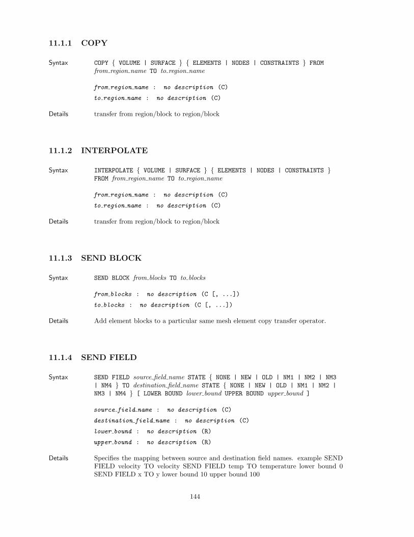
11.1.1 COPY
Syntax COPY VOLUME | SURFACE ELEMENTS | NODES | CONSTRAINTS FROMfrom region name TO to region name
from region name : no description (C)
to region name : no description (C)
Details transfer from region/block to region/block
11.1.2 INTERPOLATE
Syntax INTERPOLATE VOLUME | SURFACE ELEMENTS | NODES | CONSTRAINTS FROM from region name TO to region name
from region name : no description (C)
to region name : no description (C)
Details transfer from region/block to region/block
11.1.3 SEND BLOCK
Syntax SEND BLOCK from blocks TO to blocks
from blocks : no description (C [, ...])
to blocks : no description (C [, ...])
Details Add element blocks to a particular same mesh element copy transfer operator.
11.1.4 SEND FIELD
Syntax SEND FIELD source field name STATE NONE | NEW | OLD | NM1 | NM2 | NM3| NM4 TO destination field name STATE NONE | NEW | OLD | NM1 | NM2 |NM3 | NM4 [ LOWER BOUND lower bound UPPER BOUND upper bound ]
source field name : no description (C)
destination field name : no description (C)
lower bound : no description (R)
upper bound : no description (R)
Details Specifies the mapping between source and destination field names. example SENDFIELD velocity TO velocity SEND FIELD temp TO temperature lower bound 0SEND FIELD x TO y lower bound 10 upper bound 100
144
11.1.5 SEARCH TYPE
Details
11.1.6 NODES OUTSIDE REGION
Details
11.1.7 SEARCH COORDINATE FIELD
Syntax SEARCH COORDINATE FIELD source field name STATE NONE | NEW | OLD | NM1| NM2 | NM3 | NM4 TO destination field name STATE NONE | NEW | OLD |NM1 | NM2 | NM3 | NM4
source field name : no description (C)
destination field name : no description (C)
Details
11.1.8 SEARCH SURFACE GAP TOLERANCE
Syntax SEARCH SURFACE GAP TOLERANCE = | IS | ARE surface gap tolerance
surface gap tolerance : no description (R)
Details
11.1.9 SEARCH GEOMETRIC TOLERANCE
Syntax SEARCH GEOMETRIC TOLERANCE = | IS | ARE geometric tolerance
geometric tolerance : no description (R)
Details
11.1.10 FROM
Details Allows the send/receive mesh objects to be different.
11.1.11 INTERPOLATION FUNCTION
Syntax INTERPOLATION FUNCTION User Subroutine
User Subroutine : no description (C)
145
Details Allows an application defined subroutine to be used for the interpolation.
11.1.12 ALL FIELDS
Details Select all fields for transfer that have same name and state for source and destinationregions.
11.1.13 EXCLUDE GHOSTED
Details exclude ghosted nodes from a copy transfer
11.1.14 USE PREDEFINED TRANSFER
Syntax USE PREDEFINED TRANSFER predefined transfer name FROM from region TOto region
predefined transfer name : no description (C)
from region : no description (C)
to region : no description (C)
Details Use predefine transfer semantics provided by the specified name.
11.2 SOLUTION CONTROL DESCRIPTION
Begin SOLUTION CONTROL DESCRIPTION name
USE SYSTEM name Begin SYSTEM name
EndBegin SUBSYSTEM name
EndBegin INITIALIZE name
EndBegin PARAMETERS FOR type-name
End
146
End
Details Contains the commands needed to execute an analysis using the Calagio procedurethat utilizes Solver Control.
11.2.1 USE SYSTEM
Syntax USE SYSTEM name
name : no description (C [, ...])
Details This set the name of which system to use.
11.3 SYSTEM
Begin SYSTEM name
EVENT name [ WHEN when-expression ]
SIMULATION START TIME = | IS number
SIMULATION TERMINATION TIME = | IS number
SIMULATION MAX GLOBAL ITERATIONS = | IS number
TRANSFER name [ WHEN when-expression ]
USE INITIALIZE name
OUTPUT name [ WHEN when-expression ] Begin TRANSIENT name
EndBegin SEQUENTIAL name
End
End
Details This block wraps a solver system for a given name. The NAME parameter is thename used to define the system. There can be more than one system block in theSolver Control Description block. The ”use system NAME” line commmand controlswhich one is to be used.
147
11.3.1 EVENT
Syntax EVENT name [ WHEN when-expression ]
name : no description (C [, ...])
when-expression : no description (Q)
Details Used within a Solver Control block to indicate a single step that has no time associatedwith it. It can cause a solution transfer between regions or cause something toprint.
11.3.2 SIMULATION START TIME
Syntax SIMULATION START TIME = | IS number
number : no description (R)
Details Simulation starting time. (by default 0.0)
11.3.3 SIMULATION TERMINATION TIME
Syntax SIMULATION TERMINATION TIME = | IS number
number : no description (R)
Details The drop dead time.
11.3.4 SIMULATION MAX GLOBAL ITERATIONS
Syntax SIMULATION MAX GLOBAL ITERATIONS = | IS number
number : no description (I)
Details The Total number of Solves.
11.3.5 TRANSFER
Syntax TRANSFER name [ WHEN when-expression ]
name : no description (C [, ...])
when-expression : no description (Q)
Details A Solver Control Transfer line command which executes all transfers defined fromthe specified region. All transfers with a send region of ’name’ will be executed.
148
11.3.6 USE INITIALIZE
Syntax USE INITIALIZE name
name : no description (C [, ...])
Details This set the name of which initialization to use.
11.3.7 OUTPUT
Syntax OUTPUT name [ WHEN when-expression ]
name : no description (C [, ...])
when-expression : no description (Q)
Details A Solver Control Output line command which execute a perform I/O on the region.
11.4 TRANSIENT
Begin TRANSIENT name
ADVANCE name [ WHEN when-expression ]
EVENT name [ WHEN when-expression ]
TRANSFER name [ WHEN when-expression ]
OUTPUT name [ WHEN when-expression ]
INVOLVE name Begin NONLINEAR name
EndBegin SUBCYCLE name
EndBegin MATRIX FREE NONLINEAR name
End
End
Details This block is used to wrap a time loop.
149
11.4.1 ADVANCE
Syntax ADVANCE name [ WHEN when-expression ]
name : no description (C [, ...])
when-expression : no description (Q)
Details Used within a Solver Control block to indicate a single step that advances the solution.The name is that matches the physics.
11.4.2 EVENT
Syntax EVENT name [ WHEN when-expression ]
name : no description (C [, ...])
when-expression : no description (Q)
Details Used within a Solver Control block to indicate a single step that has no time associatedwith it. It can cause a solution transfer between regions or cause something toprint.
11.4.3 TRANSFER
Syntax TRANSFER name [ WHEN when-expression ]
name : no description (C [, ...])
when-expression : no description (Q)
Details A Solver Control Transfer line command which executes all transfers defined fromthe specified region. All transfers with a send region of ’name’ will be executed.
11.4.4 OUTPUT
Syntax OUTPUT name [ WHEN when-expression ]
name : no description (C [, ...])
when-expression : no description (Q)
Details A Solver Control Output line command which execute a perform I/O on the region.
11.4.5 INVOLVE
Syntax INVOLVE name
name : no description (C)
150
Details Specifiy a physics participant to a coupled problem solved using matrix-free nonlin-ear.
11.5 NONLINEAR
Begin NONLINEAR name
ADVANCE name [ WHEN when-expression ]
EVENT name [ WHEN when-expression ]
TRANSFER name [ WHEN when-expression ]
OUTPUT name [ WHEN when-expression ]
INVOLVE name Begin NONLINEAR name
EndBegin SUBCYCLE name
End
End
Details This block is used to wrap a nonlinear solve loop.
11.5.1 ADVANCE
Syntax ADVANCE name [ WHEN when-expression ]
name : no description (C [, ...])
when-expression : no description (Q)
Details Used within a Solver Control block to indicate a single step that advances the solution.The name is that matches the physics.
11.5.2 EVENT
Syntax EVENT name [ WHEN when-expression ]
name : no description (C [, ...])
when-expression : no description (Q)
151
Details Used within a Solver Control block to indicate a single step that has no time associatedwith it. It can cause a solution transfer between regions or cause something toprint.
11.5.3 TRANSFER
Syntax TRANSFER name [ WHEN when-expression ]
name : no description (C [, ...])
when-expression : no description (Q)
Details A Solver Control Transfer line command which executes all transfers defined fromthe specified region. All transfers with a send region of ’name’ will be executed.
11.5.4 OUTPUT
Syntax OUTPUT name [ WHEN when-expression ]
name : no description (C [, ...])
when-expression : no description (Q)
Details A Solver Control Output line command which execute a perform I/O on the region.
11.5.5 INVOLVE
Syntax INVOLVE name
name : no description (C)
Details Specifiy a physics participant to a coupled problem solved using matrix-free nonlin-ear.
11.6 NONLINEAR
Begin NONLINEAR name
End
Details This block is used to wrap a nonlinear solve loop.
152
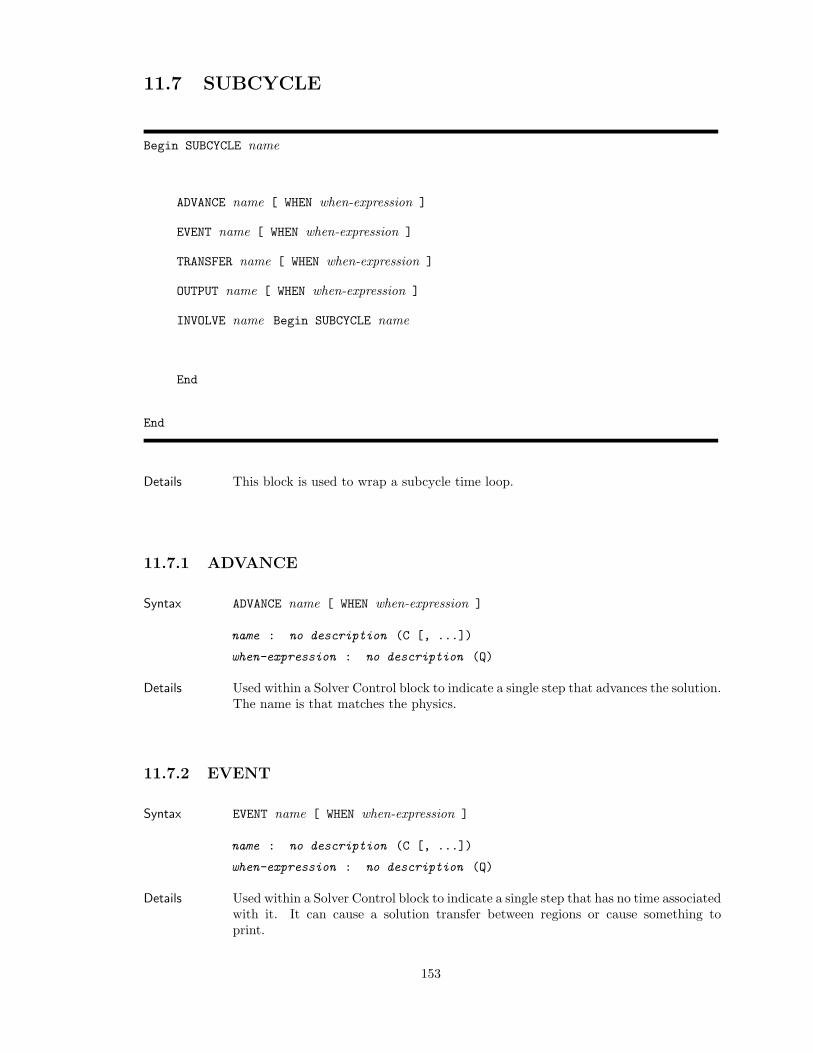
11.7 SUBCYCLE
Begin SUBCYCLE name
ADVANCE name [ WHEN when-expression ]
EVENT name [ WHEN when-expression ]
TRANSFER name [ WHEN when-expression ]
OUTPUT name [ WHEN when-expression ]
INVOLVE name Begin SUBCYCLE name
End
End
Details This block is used to wrap a subcycle time loop.
11.7.1 ADVANCE
Syntax ADVANCE name [ WHEN when-expression ]
name : no description (C [, ...])
when-expression : no description (Q)
Details Used within a Solver Control block to indicate a single step that advances the solution.The name is that matches the physics.
11.7.2 EVENT
Syntax EVENT name [ WHEN when-expression ]
name : no description (C [, ...])
when-expression : no description (Q)
Details Used within a Solver Control block to indicate a single step that has no time associatedwith it. It can cause a solution transfer between regions or cause something toprint.
153
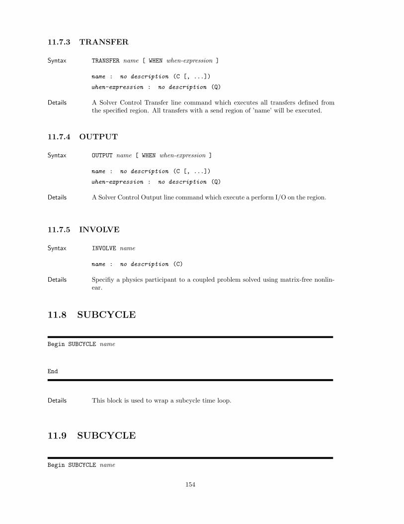
11.7.3 TRANSFER
Syntax TRANSFER name [ WHEN when-expression ]
name : no description (C [, ...])
when-expression : no description (Q)
Details A Solver Control Transfer line command which executes all transfers defined fromthe specified region. All transfers with a send region of ’name’ will be executed.
11.7.4 OUTPUT
Syntax OUTPUT name [ WHEN when-expression ]
name : no description (C [, ...])
when-expression : no description (Q)
Details A Solver Control Output line command which execute a perform I/O on the region.
11.7.5 INVOLVE
Syntax INVOLVE name
name : no description (C)
Details Specifiy a physics participant to a coupled problem solved using matrix-free nonlin-ear.
11.8 SUBCYCLE
Begin SUBCYCLE name
End
Details This block is used to wrap a subcycle time loop.
11.9 SUBCYCLE
Begin SUBCYCLE name
154
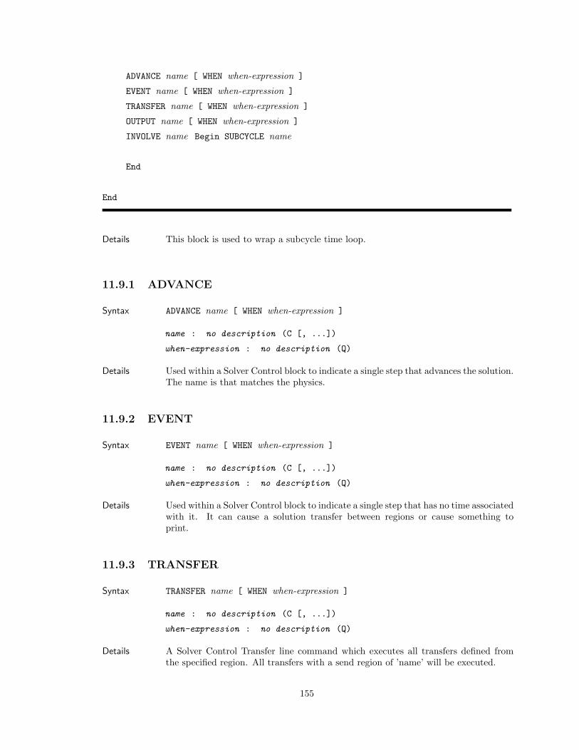
ADVANCE name [ WHEN when-expression ]
EVENT name [ WHEN when-expression ]
TRANSFER name [ WHEN when-expression ]
OUTPUT name [ WHEN when-expression ]
INVOLVE name Begin SUBCYCLE name
End
End
Details This block is used to wrap a subcycle time loop.
11.9.1 ADVANCE
Syntax ADVANCE name [ WHEN when-expression ]
name : no description (C [, ...])
when-expression : no description (Q)
Details Used within a Solver Control block to indicate a single step that advances the solution.The name is that matches the physics.
11.9.2 EVENT
Syntax EVENT name [ WHEN when-expression ]
name : no description (C [, ...])
when-expression : no description (Q)
Details Used within a Solver Control block to indicate a single step that has no time associatedwith it. It can cause a solution transfer between regions or cause something toprint.
11.9.3 TRANSFER
Syntax TRANSFER name [ WHEN when-expression ]
name : no description (C [, ...])
when-expression : no description (Q)
Details A Solver Control Transfer line command which executes all transfers defined fromthe specified region. All transfers with a send region of ’name’ will be executed.
155
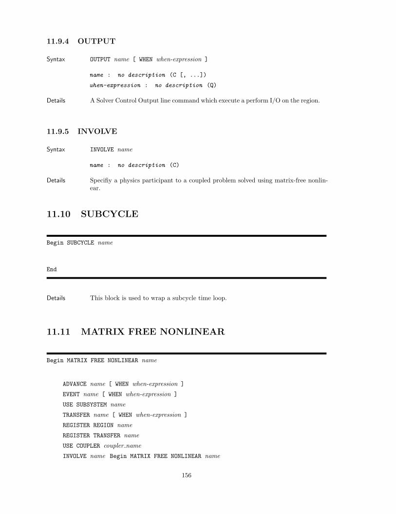
11.9.4 OUTPUT
Syntax OUTPUT name [ WHEN when-expression ]
name : no description (C [, ...])
when-expression : no description (Q)
Details A Solver Control Output line command which execute a perform I/O on the region.
11.9.5 INVOLVE
Syntax INVOLVE name
name : no description (C)
Details Specifiy a physics participant to a coupled problem solved using matrix-free nonlin-ear.
11.10 SUBCYCLE
Begin SUBCYCLE name
End
Details This block is used to wrap a subcycle time loop.
11.11 MATRIX FREE NONLINEAR
Begin MATRIX FREE NONLINEAR name
ADVANCE name [ WHEN when-expression ]
EVENT name [ WHEN when-expression ]
USE SUBSYSTEM name
TRANSFER name [ WHEN when-expression ]
REGISTER REGION name
REGISTER TRANSFER name
USE COUPLER coupler name
INVOLVE name Begin MATRIX FREE NONLINEAR name
156
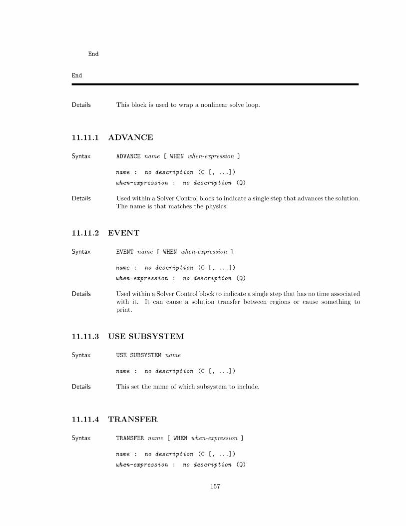
End
End
Details This block is used to wrap a nonlinear solve loop.
11.11.1 ADVANCE
Syntax ADVANCE name [ WHEN when-expression ]
name : no description (C [, ...])
when-expression : no description (Q)
Details Used within a Solver Control block to indicate a single step that advances the solution.The name is that matches the physics.
11.11.2 EVENT
Syntax EVENT name [ WHEN when-expression ]
name : no description (C [, ...])
when-expression : no description (Q)
Details Used within a Solver Control block to indicate a single step that has no time associatedwith it. It can cause a solution transfer between regions or cause something toprint.
11.11.3 USE SUBSYSTEM
Syntax USE SUBSYSTEM name
name : no description (C [, ...])
Details This set the name of which subsystem to include.
11.11.4 TRANSFER
Syntax TRANSFER name [ WHEN when-expression ]
name : no description (C [, ...])
when-expression : no description (Q)
157

Details A Solver Control Transfer line command which executes all transfers defined fromthe specified region. All transfers with a send region of ’name’ will be executed.
11.11.5 REGISTER REGION
Syntax REGISTER REGION name
name : no description (C [, ...])
Details Register 1 to many regions to participate in a Matrix Free coupled solve.
11.11.6 REGISTER TRANSFER
Syntax REGISTER TRANSFER name
name : no description (C [, ...])
Details Register 1 to many regions to participate in a Matrix Free coupled solve.
11.11.7 USE COUPLER
Syntax USE COUPLER coupler name
coupler name : no description (C)
Details Specifiy which coupler solver block to use for setting solver parameters.
11.11.8 INVOLVE
Syntax INVOLVE name
name : no description (C)
Details Specifiy a physics participant to a coupled problem solved using matrix-free nonlin-ear.
11.12 MATRIX FREE NONLINEAR
Begin MATRIX FREE NONLINEAR name
158
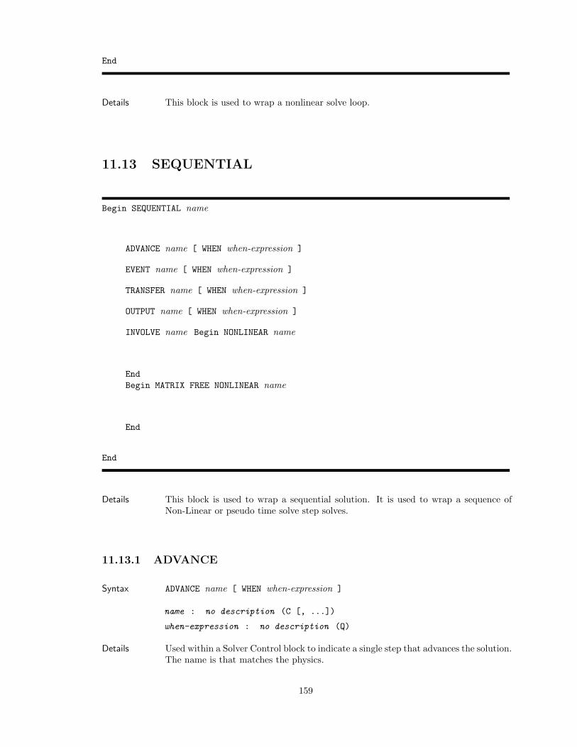
End
Details This block is used to wrap a nonlinear solve loop.
11.13 SEQUENTIAL
Begin SEQUENTIAL name
ADVANCE name [ WHEN when-expression ]
EVENT name [ WHEN when-expression ]
TRANSFER name [ WHEN when-expression ]
OUTPUT name [ WHEN when-expression ]
INVOLVE name Begin NONLINEAR name
EndBegin MATRIX FREE NONLINEAR name
End
End
Details This block is used to wrap a sequential solution. It is used to wrap a sequence ofNon-Linear or pseudo time solve step solves.
11.13.1 ADVANCE
Syntax ADVANCE name [ WHEN when-expression ]
name : no description (C [, ...])
when-expression : no description (Q)
Details Used within a Solver Control block to indicate a single step that advances the solution.The name is that matches the physics.
159
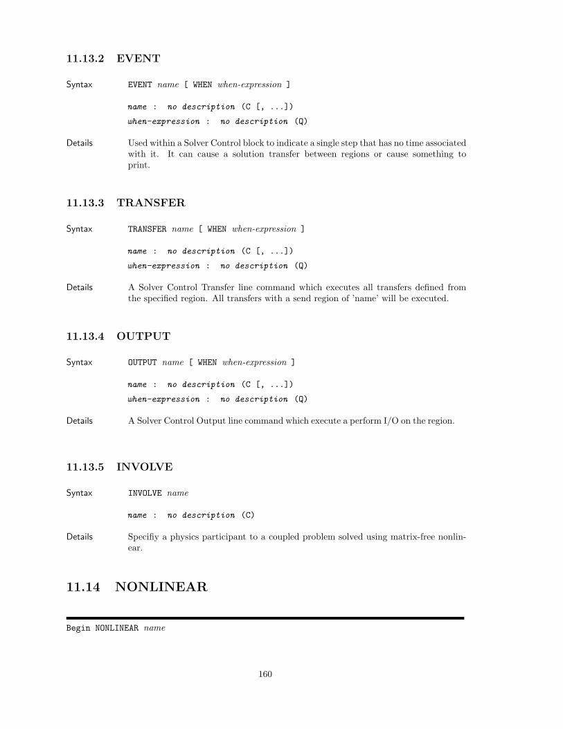
11.13.2 EVENT
Syntax EVENT name [ WHEN when-expression ]
name : no description (C [, ...])
when-expression : no description (Q)
Details Used within a Solver Control block to indicate a single step that has no time associatedwith it. It can cause a solution transfer between regions or cause something toprint.
11.13.3 TRANSFER
Syntax TRANSFER name [ WHEN when-expression ]
name : no description (C [, ...])
when-expression : no description (Q)
Details A Solver Control Transfer line command which executes all transfers defined fromthe specified region. All transfers with a send region of ’name’ will be executed.
11.13.4 OUTPUT
Syntax OUTPUT name [ WHEN when-expression ]
name : no description (C [, ...])
when-expression : no description (Q)
Details A Solver Control Output line command which execute a perform I/O on the region.
11.13.5 INVOLVE
Syntax INVOLVE name
name : no description (C)
Details Specifiy a physics participant to a coupled problem solved using matrix-free nonlin-ear.
11.14 NONLINEAR
Begin NONLINEAR name
160
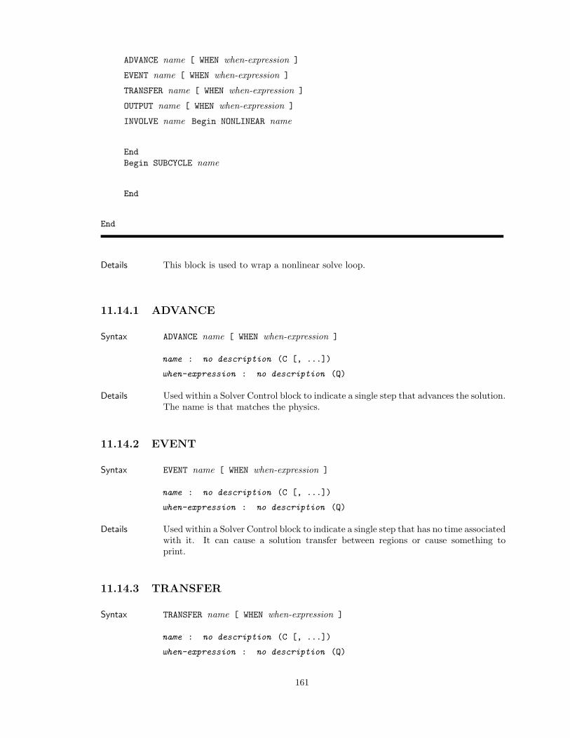
ADVANCE name [ WHEN when-expression ]
EVENT name [ WHEN when-expression ]
TRANSFER name [ WHEN when-expression ]
OUTPUT name [ WHEN when-expression ]
INVOLVE name Begin NONLINEAR name
EndBegin SUBCYCLE name
End
End
Details This block is used to wrap a nonlinear solve loop.
11.14.1 ADVANCE
Syntax ADVANCE name [ WHEN when-expression ]
name : no description (C [, ...])
when-expression : no description (Q)
Details Used within a Solver Control block to indicate a single step that advances the solution.The name is that matches the physics.
11.14.2 EVENT
Syntax EVENT name [ WHEN when-expression ]
name : no description (C [, ...])
when-expression : no description (Q)
Details Used within a Solver Control block to indicate a single step that has no time associatedwith it. It can cause a solution transfer between regions or cause something toprint.
11.14.3 TRANSFER
Syntax TRANSFER name [ WHEN when-expression ]
name : no description (C [, ...])
when-expression : no description (Q)
161
Details A Solver Control Transfer line command which executes all transfers defined fromthe specified region. All transfers with a send region of ’name’ will be executed.
11.14.4 OUTPUT
Syntax OUTPUT name [ WHEN when-expression ]
name : no description (C [, ...])
when-expression : no description (Q)
Details A Solver Control Output line command which execute a perform I/O on the region.
11.14.5 INVOLVE
Syntax INVOLVE name
name : no description (C)
Details Specifiy a physics participant to a coupled problem solved using matrix-free nonlin-ear.
11.15 NONLINEAR
Begin NONLINEAR name
End
Details This block is used to wrap a nonlinear solve loop.
11.16 SUBCYCLE
Begin SUBCYCLE name
ADVANCE name [ WHEN when-expression ]
EVENT name [ WHEN when-expression ]
TRANSFER name [ WHEN when-expression ]
OUTPUT name [ WHEN when-expression ]
162
INVOLVE name Begin SUBCYCLE name
End
End
Details This block is used to wrap a subcycle time loop.
11.16.1 ADVANCE
Syntax ADVANCE name [ WHEN when-expression ]
name : no description (C [, ...])
when-expression : no description (Q)
Details Used within a Solver Control block to indicate a single step that advances the solution.The name is that matches the physics.
11.16.2 EVENT
Syntax EVENT name [ WHEN when-expression ]
name : no description (C [, ...])
when-expression : no description (Q)
Details Used within a Solver Control block to indicate a single step that has no time associatedwith it. It can cause a solution transfer between regions or cause something toprint.
11.16.3 TRANSFER
Syntax TRANSFER name [ WHEN when-expression ]
name : no description (C [, ...])
when-expression : no description (Q)
Details A Solver Control Transfer line command which executes all transfers defined fromthe specified region. All transfers with a send region of ’name’ will be executed.
163
11.16.4 OUTPUT
Syntax OUTPUT name [ WHEN when-expression ]
name : no description (C [, ...])
when-expression : no description (Q)
Details A Solver Control Output line command which execute a perform I/O on the region.
11.16.5 INVOLVE
Syntax INVOLVE name
name : no description (C)
Details Specifiy a physics participant to a coupled problem solved using matrix-free nonlin-ear.
11.17 SUBCYCLE
Begin SUBCYCLE name
End
Details This block is used to wrap a subcycle time loop.
11.18 MATRIX FREE NONLINEAR
Begin MATRIX FREE NONLINEAR name
ADVANCE name [ WHEN when-expression ]
EVENT name [ WHEN when-expression ]
USE SUBSYSTEM name
TRANSFER name [ WHEN when-expression ]
REGISTER REGION name
REGISTER TRANSFER name
USE COUPLER coupler name
INVOLVE name Begin MATRIX FREE NONLINEAR name
164
End
End
Details This block is used to wrap a nonlinear solve loop.
11.18.1 ADVANCE
Syntax ADVANCE name [ WHEN when-expression ]
name : no description (C [, ...])
when-expression : no description (Q)
Details Used within a Solver Control block to indicate a single step that advances the solution.The name is that matches the physics.
11.18.2 EVENT
Syntax EVENT name [ WHEN when-expression ]
name : no description (C [, ...])
when-expression : no description (Q)
Details Used within a Solver Control block to indicate a single step that has no time associatedwith it. It can cause a solution transfer between regions or cause something toprint.
11.18.3 USE SUBSYSTEM
Syntax USE SUBSYSTEM name
name : no description (C [, ...])
Details This set the name of which subsystem to include.
11.18.4 TRANSFER
Syntax TRANSFER name [ WHEN when-expression ]
name : no description (C [, ...])
when-expression : no description (Q)
165
Details A Solver Control Transfer line command which executes all transfers defined fromthe specified region. All transfers with a send region of ’name’ will be executed.
11.18.5 REGISTER REGION
Syntax REGISTER REGION name
name : no description (C [, ...])
Details Register 1 to many regions to participate in a Matrix Free coupled solve.
11.18.6 REGISTER TRANSFER
Syntax REGISTER TRANSFER name
name : no description (C [, ...])
Details Register 1 to many regions to participate in a Matrix Free coupled solve.
11.18.7 USE COUPLER
Syntax USE COUPLER coupler name
coupler name : no description (C)
Details Specifiy which coupler solver block to use for setting solver parameters.
11.18.8 INVOLVE
Syntax INVOLVE name
name : no description (C)
Details Specifiy a physics participant to a coupled problem solved using matrix-free nonlin-ear.
11.19 MATRIX FREE NONLINEAR
Begin MATRIX FREE NONLINEAR name
166
End
Details This block is used to wrap a nonlinear solve loop.
11.20 SUBSYSTEM
Begin SUBSYSTEM name
ADVANCE name [ WHEN when-expression ]
EVENT name [ WHEN when-expression ]
USE SUBSYSTEM nameTRANSFER name [ WHEN when-expression ]
OUTPUT name [ WHEN when-expression ]
INVOLVE name Begin MATRIX FREE NONLINEAR name
End
End
Details This block wraps a solver subsystem for a given name. The NAME parameter isthe name used to define the system. There can be more than one system block inthe Solver Control Description block. The ”use subsystem NAME” line commmandcontrols where it will be included in a solver system.
11.20.1 ADVANCE
Syntax ADVANCE name [ WHEN when-expression ]
name : no description (C [, ...])
when-expression : no description (Q)
Details Used within a Solver Control block to indicate a single step that advances the solution.The name is that matches the physics.
11.20.2 EVENT
Syntax EVENT name [ WHEN when-expression ]
name : no description (C [, ...])
when-expression : no description (Q)
167
Details Used within a Solver Control block to indicate a single step that has no time associatedwith it. It can cause a solution transfer between regions or cause something toprint.
11.20.3 USE SUBSYSTEM
Syntax USE SUBSYSTEM name
name : no description (C [, ...])
Details This set the name of which subsystem to include.
11.20.4 TRANSFER
Syntax TRANSFER name [ WHEN when-expression ]
name : no description (C [, ...])
when-expression : no description (Q)
Details A Solver Control Transfer line command which executes all transfers defined fromthe specified region. All transfers with a send region of ’name’ will be executed.
11.20.5 OUTPUT
Syntax OUTPUT name [ WHEN when-expression ]
name : no description (C [, ...])
when-expression : no description (Q)
Details A Solver Control Output line command which execute a perform I/O on the region.
11.20.6 INVOLVE
Syntax INVOLVE name
name : no description (C)
Details Specifiy a physics participant to a coupled problem solved using matrix-free nonlin-ear.
168
11.21 MATRIX FREE NONLINEAR
Begin MATRIX FREE NONLINEAR name
ADVANCE name [ WHEN when-expression ]
EVENT name [ WHEN when-expression ]
USE SUBSYSTEM name
TRANSFER name [ WHEN when-expression ]
REGISTER REGION name
REGISTER TRANSFER name
USE COUPLER coupler name
INVOLVE name Begin MATRIX FREE NONLINEAR name
End
End
Details This block is used to wrap a nonlinear solve loop.
11.21.1 ADVANCE
Syntax ADVANCE name [ WHEN when-expression ]
name : no description (C [, ...])
when-expression : no description (Q)
Details Used within a Solver Control block to indicate a single step that advances the solution.The name is that matches the physics.
11.21.2 EVENT
Syntax EVENT name [ WHEN when-expression ]
name : no description (C [, ...])
when-expression : no description (Q)
Details Used within a Solver Control block to indicate a single step that has no time associatedwith it. It can cause a solution transfer between regions or cause something toprint.
169
11.21.3 USE SUBSYSTEM
Syntax USE SUBSYSTEM name
name : no description (C [, ...])
Details This set the name of which subsystem to include.
11.21.4 TRANSFER
Syntax TRANSFER name [ WHEN when-expression ]
name : no description (C [, ...])
when-expression : no description (Q)
Details A Solver Control Transfer line command which executes all transfers defined fromthe specified region. All transfers with a send region of ’name’ will be executed.
11.21.5 REGISTER REGION
Syntax REGISTER REGION name
name : no description (C [, ...])
Details Register 1 to many regions to participate in a Matrix Free coupled solve.
11.21.6 REGISTER TRANSFER
Syntax REGISTER TRANSFER name
name : no description (C [, ...])
Details Register 1 to many regions to participate in a Matrix Free coupled solve.
11.21.7 USE COUPLER
Syntax USE COUPLER coupler name
coupler name : no description (C)
Details Specifiy which coupler solver block to use for setting solver parameters.
170
11.21.8 INVOLVE
Syntax INVOLVE name
name : no description (C)
Details Specifiy a physics participant to a coupled problem solved using matrix-free nonlin-ear.
11.22 MATRIX FREE NONLINEAR
Begin MATRIX FREE NONLINEAR name
End
Details This block is used to wrap a nonlinear solve loop.
11.23 INITIALIZE
Begin INITIALIZE name
ADVANCE name [ WHEN when-expression ]
EVENT name [ WHEN when-expression ]
TRANSFER name [ WHEN when-expression ]
INVOLVE name
End
Details This block wraps a initializer for a given name. The NAME parameter is the nameused to define the initialization block. There can be more than one initialize blockin the Solver Control Description block. The ”use initialize NAME” line commmandcontrols which one is to be used.
11.23.1 ADVANCE
Syntax ADVANCE name [ WHEN when-expression ]
name : no description (C [, ...])
when-expression : no description (Q)
171
Details Used within a Solver Control block to indicate a single step that advances the solution.The name is that matches the physics.
11.23.2 EVENT
Syntax EVENT name [ WHEN when-expression ]
name : no description (C [, ...])
when-expression : no description (Q)
Details Used within a Solver Control block to indicate a single step that has no time associatedwith it. It can cause a solution transfer between regions or cause something toprint.
11.23.3 TRANSFER
Syntax TRANSFER name [ WHEN when-expression ]
name : no description (C [, ...])
when-expression : no description (Q)
Details A Solver Control Transfer line command which executes all transfers defined fromthe specified region. All transfers with a send region of ’name’ will be executed.
11.23.4 INVOLVE
Syntax INVOLVE name
name : no description (C)
Details Specifiy a physics participant to a coupled problem solved using matrix-free nonlin-ear.
11.24 PARAMETERS FOR
Begin PARAMETERS FOR type-name
TARGET ERROR FOR region-name MeshObjectType field-name = | IS target-number
INITIAL DELTAT = | IS number
TERMINATION TIME = | IS number
TOTAL CHANGE IN TIME = | IS number
NUMBER OF STEPS = | IS number
START TIME = | IS number
172
CONVERGED WHEN convergence-expressionTIME STEP STYLE TimeStepStyle Begin PARAMETERS FOR ARIA REGION RegionName
End
End
Details A Solver Control PARAMETERS block to set up control data for the SC type param-eter. Inside this block one sets the time step parameters or nonlinear parameters.
11.24.1 TARGET ERROR FOR
Syntax TARGET ERROR FOR region-name MeshObjectType field-name = | IS target-number
region-name : no description (C)
field-name : no description (C)
target-number : no description (R)
Details Assign a target number for a mesh object in a region for convergence.
11.24.2 INITIAL DELTAT
Syntax INITIAL DELTAT = | IS number
number : no description (R)
Details Assign an initial delta T
11.24.3 TERMINATION TIME
Syntax TERMINATION TIME = | IS number
number : no description (R)
Details Assign a final time to stop
11.24.4 TOTAL CHANGE IN TIME
Syntax TOTAL CHANGE IN TIME = | IS number
number : no description (R)
173
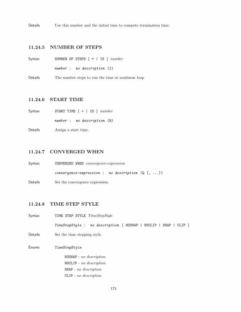
Details Use this number and the initial time to compute termination time.
11.24.5 NUMBER OF STEPS
Syntax NUMBER OF STEPS = | IS number
number : no description (I)
Details The number steps to run the time or nonlinear loop
11.24.6 START TIME
Syntax START TIME = | IS number
number : no description (R)
Details Assign a start time.
11.24.7 CONVERGED WHEN
Syntax CONVERGED WHEN convergence-expression
convergence-expression : no description (Q [, ...])
Details Set the convergence expression.
11.24.8 TIME STEP STYLE
Syntax TIME STEP STYLE TimeStepStyle
TimeStepStyle : no description NOSNAP | NOCLIP | SNAP | CLIP
Details Set the time stepping style.
Enums TimeStepStyle
NOSNAP - no description
NOCLIP - no description
SNAP - no description
CLIP - no description
174
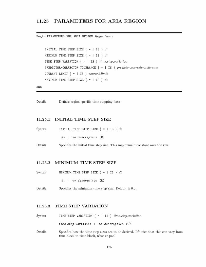
11.25 PARAMETERS FOR ARIA REGION
Begin PARAMETERS FOR ARIA REGION RegionName
INITIAL TIME STEP SIZE = | IS dt
MINIMUM TIME STEP SIZE = | IS dt
TIME STEP VARIATION = | IS time step variation
PREDICTOR-CORRECTOR TOLERANCE = | IS predictor corrector tolerance
COURANT LIMIT = | IS courant limit
MAXIMUM TIME STEP SIZE = | IS dt
End
Details Defines region specific time stepping data
11.25.1 INITIAL TIME STEP SIZE
Syntax INITIAL TIME STEP SIZE = | IS dt
dt : no description (R)
Details Specifies the initial time step size. This may remain constant over the run.
11.25.2 MINIMUM TIME STEP SIZE
Syntax MINIMUM TIME STEP SIZE = | IS dt
dt : no description (R)
Details Specifies the minimum time step size. Default is 0.0.
11.25.3 TIME STEP VARIATION
Syntax TIME STEP VARIATION = | IS time step variation
time step variation : no description (C)
Details Specifies how the time step sizes are to be derived. It’s nice that this can vary fromtime block to time block, n’est ce pas?
175
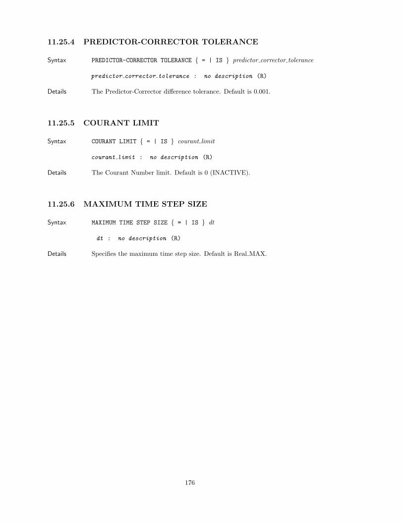
11.25.4 PREDICTOR-CORRECTOR TOLERANCE
Syntax PREDICTOR-CORRECTOR TOLERANCE = | IS predictor corrector tolerance
predictor corrector tolerance : no description (R)
Details The Predictor-Corrector difference tolerance. Default is 0.001.
11.25.5 COURANT LIMIT
Syntax COURANT LIMIT = | IS courant limit
courant limit : no description (R)
Details The Courant Number limit. Default is 0 (INACTIVE).
11.25.6 MAXIMUM TIME STEP SIZE
Syntax MAXIMUM TIME STEP SIZE = | IS dt
dt : no description (R)
Details Specifies the maximum time step size. Default is Real MAX.
176
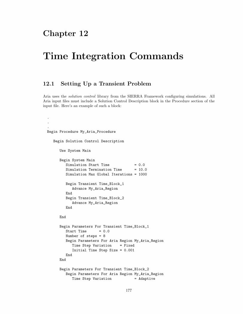
Chapter 12
Time Integration Commands
12.1 Setting Up a Transient Problem
Aria uses the solution control library from the SIERRA Framework configuring simulations. AllAria input files must include a Solution Control Description block in the Procedure section of theinput file. Here’s an example of such a block:
.
.
.Begin Procedure My_Aria_Procedure
Begin Solution Control Description
Use System Main
Begin System MainSimulation Start Time = 0.0Simulation Termination Time = 10.0Simulation Max Global Iterations = 1000
Begin Transient Time_Block_1Advance My_Aria_Region
EndBegin Transient Time_Block_2
Advance My_Aria_RegionEnd
End
Begin Parameters For Transient Time_Block_1Start Time = 0.0Number of steps = 8Begin Parameters For Aria Region My_Aria_Region
Time Step Variation = FixedInitial Time Step Size = 0.001
EndEnd
Begin Parameters For Transient Time_Block_2Begin Parameters For Aria Region My_Aria_Region
Time Step Variation = Adaptive
177
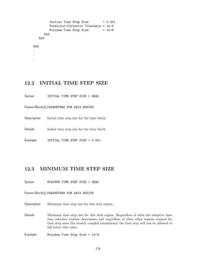
Initial Time Step Size = 0.001Predictor-Corrector Tolerance = 1e-3Minimum Time Step Size = 1e-6
EndEnd
End...
12.2 INITIAL TIME STEP SIZE
Syntax INITIAL TIME STEP SIZE = REAL
Parent Block(s) PARAMETERS FOR ARIA REGION
Description Initial time step size for the time block.
Details Initial time step size for the time block.
Example INITIAL TIME STEP SIZE = 0.001
12.3 MINIMUM TIME STEP SIZE
Syntax MINIMUM TIME STEP SIZE = REAL
Parent Block(s) PARAMETERS FOR ARIA REGION
Description Minimum time step size for this Aria region.
Details Minimum time step size for this Aria region. Regardless of what the adaptive timestep selection routine determines and regardless of what other regions request fortime step sizes (for loosely coupled simulations) the time step will not be allowed tofall below this value.
Example Minimum Time Step Size = 1e-8
178
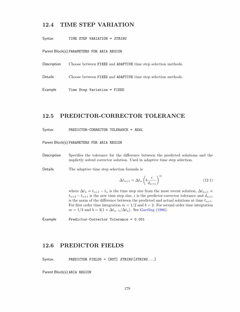
12.4 TIME STEP VARIATION
Syntax TIME STEP VARIATION = STRING
Parent Block(s) PARAMETERS FOR ARIA REGION
Description Choose between FIXED and ADAPTIVE time step selection methods.
Details Choose between FIXED and ADAPTIVE time step selection methods.
Example Time Step Variation = FIXED
12.5 PREDICTOR-CORRECTOR TOLERANCE
Syntax PREDICTOR-CORRECTOR TOLERANCE = REAL
Parent Block(s) PARAMETERS FOR ARIA REGION
Description Specifies the tolerance for the difference between the predicted solutiona and theimplictly solved corrector solution. Used in adaptive time step selection.
Details The adaptive time step selection formula is
∆tn+1 = ∆tn
(b
ε
dn+1
)m
(12.1)
where ∆tn ≡ tn+1 − tn is the time step size from the most recent solution, ∆tn+1 ≡tn+2 − tn+1 is the new time step size, ε is the predictor-corrector tolerance and dn+1
is the norm of the difference between the predicted and actual solutions at time tn+1.For first order time integration m = 1/2 and b = 2. For second order time integrationm = 1/3 and b = 3(1 + ∆tn−1/∆tn). See Gartling (1986).
Example Predictor-Corrector Tolerance = 0.001
12.6 PREDICTOR FIELDS
Syntax PREDICTOR FIELDS = [NOT] STRING [STRING ...]
Parent Block(s) ARIA REGION
179
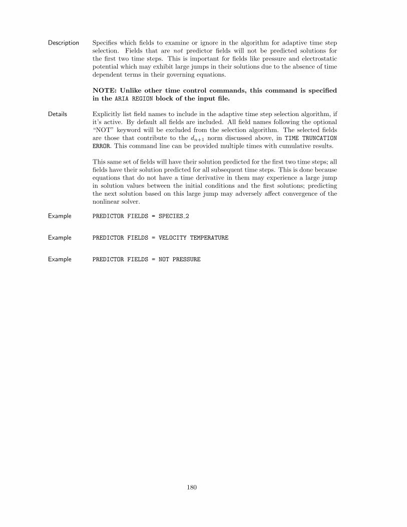
Description Specifies which fields to examine or ignore in the algorithm for adaptive time stepselection. Fields that are not predictor fields will not be predicted solutions forthe first two time steps. This is important for fields like pressure and electrostaticpotential which may exhibit large jumps in their solutions due to the absence of timedependent terms in their governing equations.
NOTE: Unlike other time control commands, this command is specifiedin the ARIA REGION block of the input file.
Details Explicitly list field names to include in the adaptive time step selection algorithm, ifit’s active. By default all fields are included. All field names following the optional“NOT” keyword will be excluded from the selection algorithm. The selected fieldsare those that contribute to the dn+1 norm discussed above, in TIME TRUNCATIONERROR. This command line can be provided multiple times with cumulative results.
This same set of fields will have their solution predicted for the first two time steps; allfields have their solution predicted for all subsequent time steps. This is done becauseequations that do not have a time derivative in them may experience a large jumpin solution values between the initial conditions and the first solutions; predictingthe next solution based on this large jump may adversely affect convergence of thenonlinear solver.
Example PREDICTOR FIELDS = SPECIES 2
Example PREDICTOR FIELDS = VELOCITY TEMPERATURE
Example PREDICTOR FIELDS = NOT PRESSURE
180
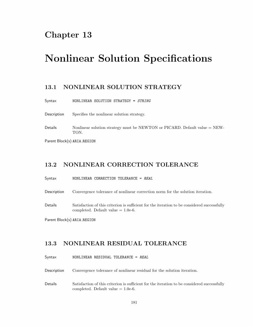
Chapter 13
Nonlinear Solution Specifications
13.1 NONLINEAR SOLUTION STRATEGY
Syntax NONLINEAR SOLUTION STRATEGY = STRING
Description Specifies the nonlinear solution strategy.
Details Nonlinear solution strategy must be NEWTON or PICARD. Default value = NEW-TON.
Parent Block(s) ARIA REGION
13.2 NONLINEAR CORRECTION TOLERANCE
Syntax NONLINEAR CORRECTION TOLERANCE = REAL
Description Convergence tolerance of nonlinear correction norm for the solution iteration.
Details Satisfaction of this criterion is sufficient for the iteration to be considered successfullycompleted. Default value = 1.0e-6.
Parent Block(s) ARIA REGION
13.3 NONLINEAR RESIDUAL TOLERANCE
Syntax NONLINEAR RESIDUAL TOLERANCE = REAL
Description Convergence tolerance of nonlinear residual for the solution iteration.
Details Satisfaction of this criterion is sufficient for the iteration to be considered successfullycompleted. Default value = 1.0e-6.
181
Parent Block(s) ARIA REGION
13.4 NONLINEAR RESIDUAL RATIO TOLERANCE
Syntax NONLINEAR RESIDUAL RATIO TOLERANCE = REAL
Description Convergence tolerance of ratio of the nonlinear residual to the initial nonlinear resid-ual for the solution iteration.
Details Satisfaction of this criterion is sufficient for the iteration to be considered successfullycompleted. Default value = 0.0
Parent Block(s) ARIA REGION
13.5 NONLINEAR RELAXATION FACTOR
Syntax NONLINEAR RELAXATION FACTOR = REAL
Description Weighting factor for fraction of a new nonlinear solution that will be applied to thelinear solution update.
Details Weighting factor lies in the range 0.0 to 1.0. Default value = 1.0.
Parent Block(s) ARIA REGION
13.6 MAXIMUM NONLINEAR ITERATIONS
Syntax MAXIMUM NONLINEAR ITERATIONS = INT
Description Number of allowable nonlinear iterations in one linear solution step.
Details The solution step will terminate when the number of nonlinear iterations are exceeded.Default value = 20.
Parent Block(s) ARIA REGION
182
13.7 MINIMUM NONLINEAR ITERATIONS
Syntax MINIMUM NONLINEAR ITERATIONS = INT
Description Minimum number of nonlinear iterations required.
Details The nonlinear solver will continue iterating until this minimum number of iterationsare performed, including solving the nonlinear matrix system. The default value isone (1) but setting this to zero can be useful for some situations.
Parent Block(s) ARIA REGION
13.8 ACCEPT SOLUTION AFTER MAXIMUM NONLIN-EAR ITERATIONS
Syntax ACCEPT SOLUTION AFTER MAXIMUM NONLINEAR ITERATIONS = BOOL
Description Determines whether reaching the maximum number of nonlinear iterations is a “suc-cess” criterion.
Details Determines whether reaching the maximum number of nonlinear iterations is a “suc-cess” criterion. By default, this is false. By the way, valid values of BOOL are TRUEand FALSE, case insensitive.
Parent Block(s) ARIA REGION
13.9 FILTER NONLINEAR SOLUTION
Syntax FILTER NONLINEAR SOLUTION FOR DOF FILTER TYPE = REAL 1 REAL 2
Description Restrict the value of a solution variable used in the nonlinear solver iterations of asolution step.
Details The nonlinear solution can be restricted to a range with upper and lower limits usingthe FILTER TYPE = RANGE while supplying two bounding values. To set an upperor lower bound use FILTER TYPE = MAXIMUM or FILTER TYPE = MINIMUMwhile supplying a single bounding value.
Parent Block(s) ARIA REGION
183

184
Chapter 14
Writing User Plugins
14.1 About Plugins
Users are free to extend Aria’s library of material models, constitutive equations, boundary condi-tions, distinguishing conditions and source terms through the use of plugins. In order to do this,a user writes the C++ code to implement an Expression class. Before delving into Aria pluginsit’s worth reading section 23.1 and scanning section 23.4 for an introduction to Aria’s Expressionsystem.
When a user supplies their own plugin it becomes a first-class piece of Aria. Plugins have noperformance penalty over Aria’s built-in functionality and plugins have no added restrictions overbuilt-in Expression regarding what can and can’t be done. In fact, taking a user plugin and addingit to Aria proper (so that it becomes “owned” by Aria) is a piece of cake.
It’s worth re-stating here that a lot of Aria’s algorithms make use of sensitivities, i.e., Aria often needsto know the derivative of your model with respect to all of the unknowns in the problem. There arethree ways to supply the sensitivities in aria: write them by hand, use a numerical finite-differencefunction, or use (forward) automatic differentiation (FAD). The FAD method is ideal for pluginsbecause the sensitivities are are analytical and exact though there may be a small performancedegradation. However, if only a few models use FAD there may be no measurable performance hit.For that reason, we’ve designed our plugin system to use FAD by default. If you have differentneeds, contact the developers for help.
14.2 Compiling and Using Plugins
Let’s say that we have plugin C++ code for our very own density model in a file named My Density.C.In order to use this plugin we’ll first need to build it into Aria and to do that we’ll need a projectwhere we can build Aria. Here are the basic steps:
% cd ~/projects/
% create project -s SierraVOTD plugin project
% cd plugin project
% checkout --deps aria
Now, currently there’s a restriction that your plugin has to be stored in the aria/ subdirectory ofyour project. We’ll fix that eventually but in the mean time we need to put our plugin code there,e.g.,
185
% mkdir aria
% cp /some/path/My Density.C aria
% build PLUGINS=My Density.C
To compile-in our plugin we use a Makefile variable called PLUGINS. We can place this right on theSNTools’ build command line like this:
% build PLUGINS=My Density.C aria
Naturally, other options to build can be added to the command line.
Running the pluginified Aria executable can be done as normal using the SNTools’ sierra tool. Ifyour input files are somewhere inside the project where you built your plugin then you can run thesierra tool as normal. If your input files are somewhere else, you can use the -x project-path
option to sierra to tell it to use your project. Continuing our example,
% cd ~/some/other/path
% sierra aria -i use my density.i -x ~/projects/plugin project
14.3 An Important Note About Model Names
In order to avoid name clashes, model names always end with the generic name of the quantity theyprovide. So, density model names always end in DENSITY, viscosity model names end in VISCOSITY,etc. For material models, it’s easy to know what that ending is because it’s the same as the left-handside of the “=” sign in the material input block (with spaces replaced by an underscore “ ”). Forsource terms, it’s always the name of the equation plus SOURCE, e.g., ENERGY SOURCE. Clearly, it’simportant to keep this in mind when naming and referring to your plugin model or else Aria won’tbe able to find it properly.
In this example, we’ll name our density MY MODEL DENSITY (recall, it must end in DENSITY) so inthe input file we’ll have to refer to it as MY MODEL since the ending is automatically added.
14.4 The Input File
Plugins can be referenced in the input file similiar to the way Aria’s built-in Expressions are ref-erenced. The name of the model is just whatever your plugin is named without the endign, e.g.,MY MODEL,
Begin Aria Material KryptoniteDensity = My_Model a=1.0 b=-0.01...
End
It’s important to note that the plugin name must not conflict with model names used internally byAria (the outcome would be, at least to users, ambiguous). Aria will verify this and produce anderror if there’s a name clash.
186
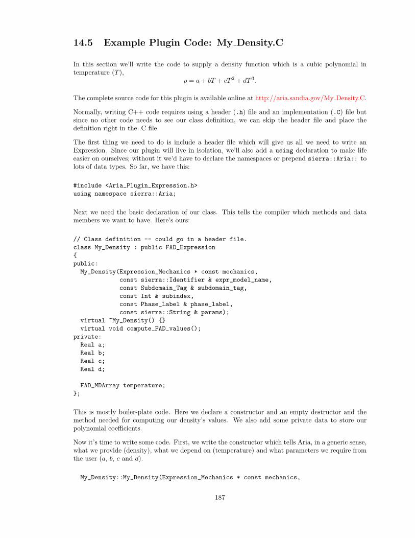
14.5 Example Plugin Code: My Density.C
In this section we’ll write the code to supply a density function which is a cubic polynomial intemperature (T ),
ρ = a + bT + cT 2 + dT 3.
The complete source code for this plugin is available online at http://aria.sandia.gov/My Density.C.
Normally, writing C++ code requires using a header (.h) file and an implementation (.C) file butsince no other code needs to see our class definition, we can skip the header file and place thedefinition right in the .C file.
The first thing we need to do is include a header file which will give us all we need to write anExpression. Since our plugin will live in isolation, we’ll also add a using declaration to make lifeeasier on ourselves; without it we’d have to declare the namespaces or prepend sierra::Aria:: tolots of data types. So far, we have this:
#include <Aria_Plugin_Expression.h>using namespace sierra::Aria;
Next we need the basic declaration of our class. This tells the compiler which methods and datamembers we want to have. Here’s ours:
// Class definition -- could go in a header file.class My_Density : public FAD_Expressionpublic:My_Density(Expression_Mechanics * const mechanics,
const sierra::Identifier & expr_model_name,const Subdomain_Tag & subdomain_tag,const Int & subindex,const Phase_Label & phase_label,const sierra::String & params);
virtual ~My_Density() virtual void compute_FAD_values();
private:Real a;Real b;Real c;Real d;
FAD_MDArray temperature;;
This is mostly boiler-plate code. Here we declare a constructor and an empty destructor and themethod needed for computing our density’s values. We also add some private data to store ourpolynomial coefficients.
Now it’s time to write some code. First, we write the constructor which tells Aria, in a generic sense,what we provide (density), what we depend on (temperature) and what parameters we require fromthe user (a, b, c and d).
My_Density::My_Density(Expression_Mechanics * const mechanics,
187
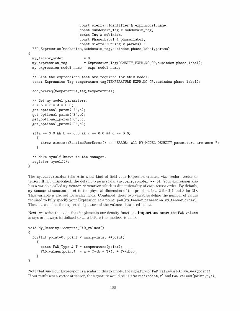
const sierra::Identifier & expr_model_name,const Subdomain_Tag & subdomain_tag,const Int & subindex,const Phase_Label & phase_label,const sierra::String & params) :
FAD_Expression(mechanics,subdomain_tag,subindex,phase_label,params)my_tensor_order = 0;my_expression_tag = Expression_Tag(DENSITY_EXPR,NO_OP,subindex,phase_label);my_expression_model_name = expr_model_name;
// List the expressions that are required for this model.const Expression_Tag temperature_tag(TEMPERATURE_EXPR,NO_OP,subindex,phase_label);
add_prereq(temperature_tag,temperature);
// Get my model parameters.a = b = c = d = 0.0;get_optional_param("A",a);get_optional_param("B",b);get_optional_param("C",c);get_optional_param("D",d);
if(a == 0.0 && b == 0.0 && c == 0.0 && d == 0.0)throw sierra::RuntimeUserError() << "ERROR: All MY_MODEL_DENSITY parameters are zero.";
// Make myself known to the manager.register_myself();
The my tensor order tells Aria what kind of field your Expresion creates, viz. scalar, vector ortensor. If left unspecified, the default type is scalar (my tensor order == 0). Your expression alsohas a variable called my tensor dimension which is dimensionality of each tensor order. By default,my tensor dimension is set to the physical dimension of the problem, i.e., 2 for 2D and 3 for 3D.This variable is also set for scalar fields. Combined, these two variables define the number of valuesrequired to fully specify your Expression at a point: pow(my tensor dimension,my tensor order).These also define the expected signature of the values data used below.
Next, we write the code that implements our density function. Important note: the FAD valuesarrays are always initialized to zero before this method is called.
void My_Density::compute_FAD_values()for(Int point=0; point < num_points; ++point)const FAD_Type & T = temperature(point);FAD_values(point) = a + T*(b + T*(c + T*(d)));
Note that since our Expression is a scalar in this example, the signature of FAD values is FAD values(point).If our result was a vector or tensor, the signature would be FAD values(point,r) and FAD values(point,r,s),
188
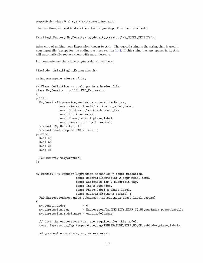
respectively, where 0 ≤ r,s < my tensor dimension.
The last thing we need to do is the actual plugin step. This one line of code,
ExprPluginFactory<My_Density> my_density_creator("MY_MODEL_DENSITY");
takes care of making your Expression known to Aria. The quoted string is the string that is used inyour input file (except for the ending part, see section 14.3. If this string has any spaces in it, Ariawill automatically replace them with an underscore.
For completeness the whole plugin code is given here.
#include <Aria_Plugin_Expression.h>
using namespace sierra::Aria;
// Class definition -- could go in a header file.class My_Density : public FAD_Expressionpublic:My_Density(Expression_Mechanics * const mechanics,
const sierra::Identifier & expr_model_name,const Subdomain_Tag & subdomain_tag,const Int & subindex,const Phase_Label & phase_label,const sierra::String & params);
virtual ~My_Density() virtual void compute_FAD_values();
private:Real a;Real b;Real c;Real d;
FAD_MDArray temperature;;
My_Density::My_Density(Expression_Mechanics * const mechanics,const sierra::Identifier & expr_model_name,const Subdomain_Tag & subdomain_tag,const Int & subindex,const Phase_Label & phase_label,const sierra::String & params) :
FAD_Expression(mechanics,subdomain_tag,subindex,phase_label,params)my_tensor_order = 0;my_expression_tag = Expression_Tag(DENSITY_EXPR,NO_OP,subindex,phase_label);my_expression_model_name = expr_model_name;
// List the expressions that are required for this model.const Expression_Tag temperature_tag(TEMPERATURE_EXPR,NO_OP,subindex,phase_label);
add_prereq(temperature_tag,temperature);
189
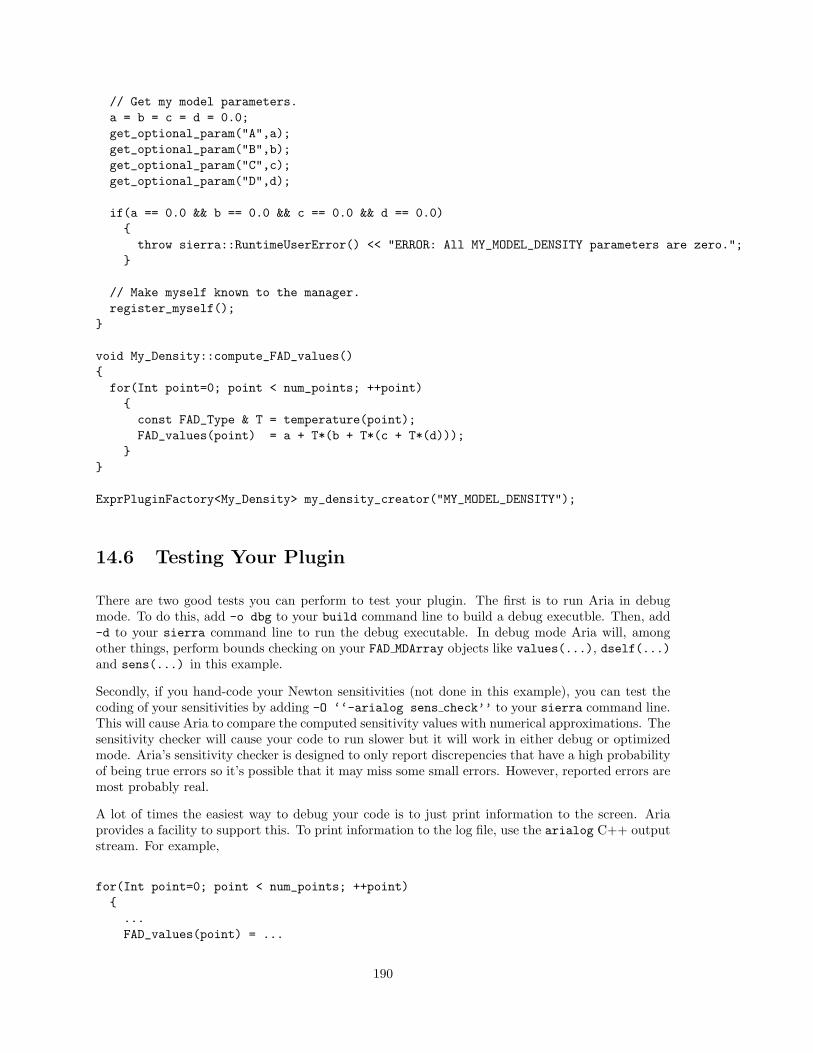
// Get my model parameters.a = b = c = d = 0.0;get_optional_param("A",a);get_optional_param("B",b);get_optional_param("C",c);get_optional_param("D",d);
if(a == 0.0 && b == 0.0 && c == 0.0 && d == 0.0)throw sierra::RuntimeUserError() << "ERROR: All MY_MODEL_DENSITY parameters are zero.";
// Make myself known to the manager.register_myself();
void My_Density::compute_FAD_values()for(Int point=0; point < num_points; ++point)const FAD_Type & T = temperature(point);FAD_values(point) = a + T*(b + T*(c + T*(d)));
ExprPluginFactory<My_Density> my_density_creator("MY_MODEL_DENSITY");
14.6 Testing Your Plugin
There are two good tests you can perform to test your plugin. The first is to run Aria in debugmode. To do this, add -o dbg to your build command line to build a debug executble. Then, add-d to your sierra command line to run the debug executable. In debug mode Aria will, amongother things, perform bounds checking on your FAD MDArray objects like values(...), dself(...)and sens(...) in this example.
Secondly, if you hand-code your Newton sensitivities (not done in this example), you can test thecoding of your sensitivities by adding -O ‘‘-arialog sens check’’ to your sierra command line.This will cause Aria to compare the computed sensitivity values with numerical approximations. Thesensitivity checker will cause your code to run slower but it will work in either debug or optimizedmode. Aria’s sensitivity checker is designed to only report discrepencies that have a high probabilityof being true errors so it’s possible that it may miss some small errors. However, reported errors aremost probably real.
A lot of times the easiest way to debug your code is to just print information to the screen. Ariaprovides a facility to support this. To print information to the log file, use the arialog C++ outputstream. For example,
for(Int point=0; point < num_points; ++point)...FAD_values(point) = ...
190
arialog.m(LOG_PLUGIN) << "value(" << point << ") = " << value(point) << endl;
Then, you can activate this output by adding the option -O ‘‘-arialog plugin’’ to your sierracommand line. If you leave off the .m(LOG PLUGIN) part then it will always write your output tothe log file. There’s a performance penalty for having this code present (even if out don’t turn thelogging on) so you probably want to remove it once you’re done debugging.
191

192
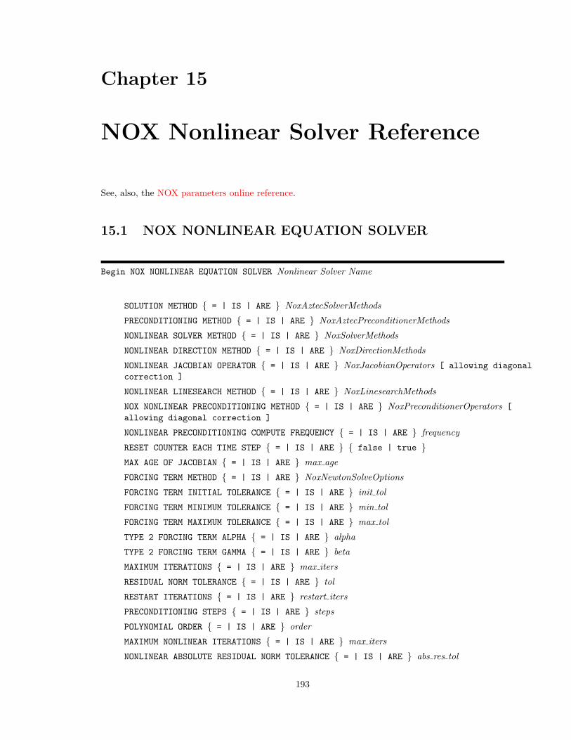
Chapter 15
NOX Nonlinear Solver Reference
See, also, the NOX parameters online reference.
15.1 NOX NONLINEAR EQUATION SOLVER
Begin NOX NONLINEAR EQUATION SOLVER Nonlinear Solver Name
SOLUTION METHOD = | IS | ARE NoxAztecSolverMethods
PRECONDITIONING METHOD = | IS | ARE NoxAztecPreconditionerMethods
NONLINEAR SOLVER METHOD = | IS | ARE NoxSolverMethods
NONLINEAR DIRECTION METHOD = | IS | ARE NoxDirectionMethods
NONLINEAR JACOBIAN OPERATOR = | IS | ARE NoxJacobianOperators [ allowing diagonalcorrection ]
NONLINEAR LINESEARCH METHOD = | IS | ARE NoxLinesearchMethods
NOX NONLINEAR PRECONDITIONING METHOD = | IS | ARE NoxPreconditionerOperators [allowing diagonal correction ]
NONLINEAR PRECONDITIONING COMPUTE FREQUENCY = | IS | ARE frequency
RESET COUNTER EACH TIME STEP = | IS | ARE false | true MAX AGE OF JACOBIAN = | IS | ARE max age
FORCING TERM METHOD = | IS | ARE NoxNewtonSolveOptions
FORCING TERM INITIAL TOLERANCE = | IS | ARE init tol
FORCING TERM MINIMUM TOLERANCE = | IS | ARE min tol
FORCING TERM MAXIMUM TOLERANCE = | IS | ARE max tol
TYPE 2 FORCING TERM ALPHA = | IS | ARE alpha
TYPE 2 FORCING TERM GAMMA = | IS | ARE beta
MAXIMUM ITERATIONS = | IS | ARE max iters
RESIDUAL NORM TOLERANCE = | IS | ARE tol
RESTART ITERATIONS = | IS | ARE restart iters
PRECONDITIONING STEPS = | IS | ARE steps
POLYNOMIAL ORDER = | IS | ARE order
MAXIMUM NONLINEAR ITERATIONS = | IS | ARE max iters
NONLINEAR ABSOLUTE RESIDUAL NORM TOLERANCE = | IS | ARE abs res tol
193
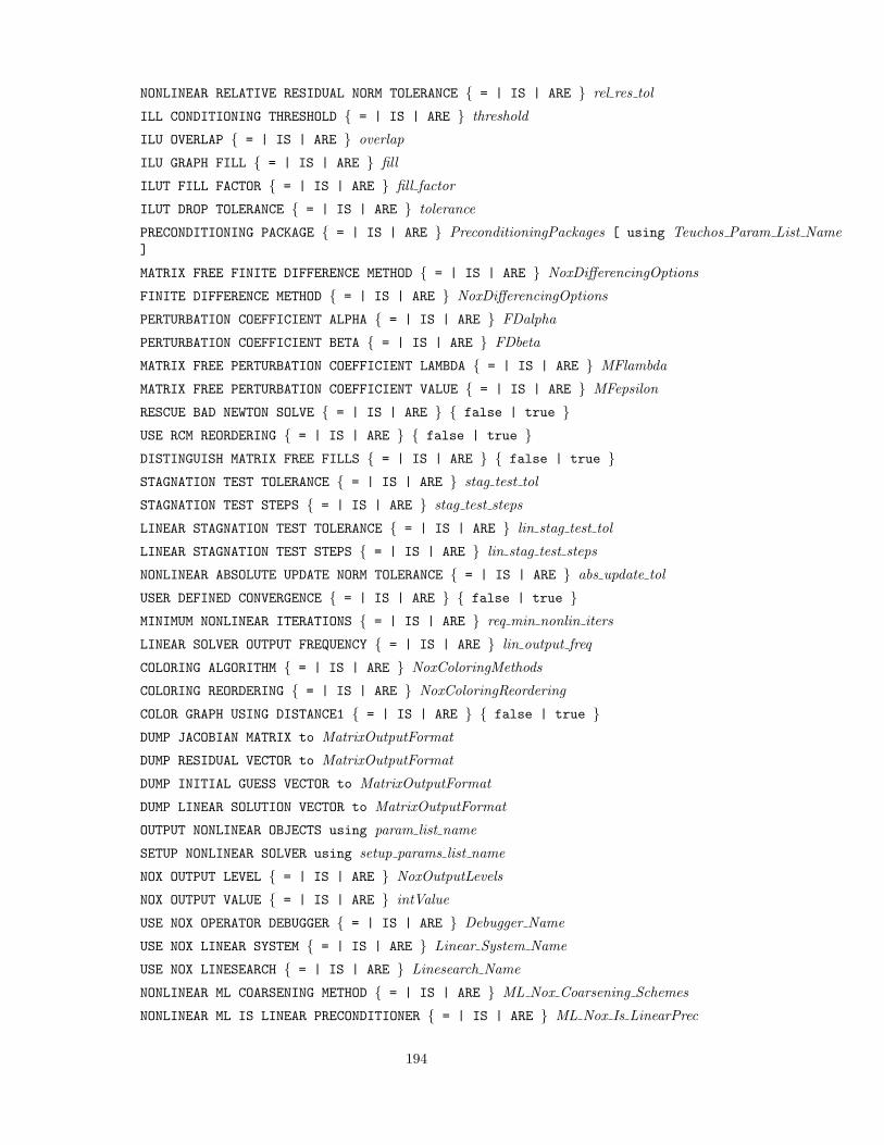
NONLINEAR RELATIVE RESIDUAL NORM TOLERANCE = | IS | ARE rel res tol
ILL CONDITIONING THRESHOLD = | IS | ARE threshold
ILU OVERLAP = | IS | ARE overlap
ILU GRAPH FILL = | IS | ARE fill
ILUT FILL FACTOR = | IS | ARE fill factor
ILUT DROP TOLERANCE = | IS | ARE tolerance
PRECONDITIONING PACKAGE = | IS | ARE PreconditioningPackages [ using Teuchos Param List Name]
MATRIX FREE FINITE DIFFERENCE METHOD = | IS | ARE NoxDifferencingOptions
FINITE DIFFERENCE METHOD = | IS | ARE NoxDifferencingOptions
PERTURBATION COEFFICIENT ALPHA = | IS | ARE FDalpha
PERTURBATION COEFFICIENT BETA = | IS | ARE FDbeta
MATRIX FREE PERTURBATION COEFFICIENT LAMBDA = | IS | ARE MFlambda
MATRIX FREE PERTURBATION COEFFICIENT VALUE = | IS | ARE MFepsilon
RESCUE BAD NEWTON SOLVE = | IS | ARE false | true USE RCM REORDERING = | IS | ARE false | true DISTINGUISH MATRIX FREE FILLS = | IS | ARE false | true STAGNATION TEST TOLERANCE = | IS | ARE stag test tol
STAGNATION TEST STEPS = | IS | ARE stag test steps
LINEAR STAGNATION TEST TOLERANCE = | IS | ARE lin stag test tol
LINEAR STAGNATION TEST STEPS = | IS | ARE lin stag test steps
NONLINEAR ABSOLUTE UPDATE NORM TOLERANCE = | IS | ARE abs update tol
USER DEFINED CONVERGENCE = | IS | ARE false | true MINIMUM NONLINEAR ITERATIONS = | IS | ARE req min nonlin iters
LINEAR SOLVER OUTPUT FREQUENCY = | IS | ARE lin output freq
COLORING ALGORITHM = | IS | ARE NoxColoringMethods
COLORING REORDERING = | IS | ARE NoxColoringReordering
COLOR GRAPH USING DISTANCE1 = | IS | ARE false | true DUMP JACOBIAN MATRIX to MatrixOutputFormat
DUMP RESIDUAL VECTOR to MatrixOutputFormat
DUMP INITIAL GUESS VECTOR to MatrixOutputFormat
DUMP LINEAR SOLUTION VECTOR to MatrixOutputFormat
OUTPUT NONLINEAR OBJECTS using param list name
SETUP NONLINEAR SOLVER using setup params list name
NOX OUTPUT LEVEL = | IS | ARE NoxOutputLevels
NOX OUTPUT VALUE = | IS | ARE intValue
USE NOX OPERATOR DEBUGGER = | IS | ARE Debugger Name
USE NOX LINEAR SYSTEM = | IS | ARE Linear System Name
USE NOX LINESEARCH = | IS | ARE Linesearch Name
NONLINEAR ML COARSENING METHOD = | IS | ARE ML Nox Coarsening Schemes
NONLINEAR ML IS LINEAR PRECONDITIONER = | IS | ARE ML Nox Is LinearPrec
194
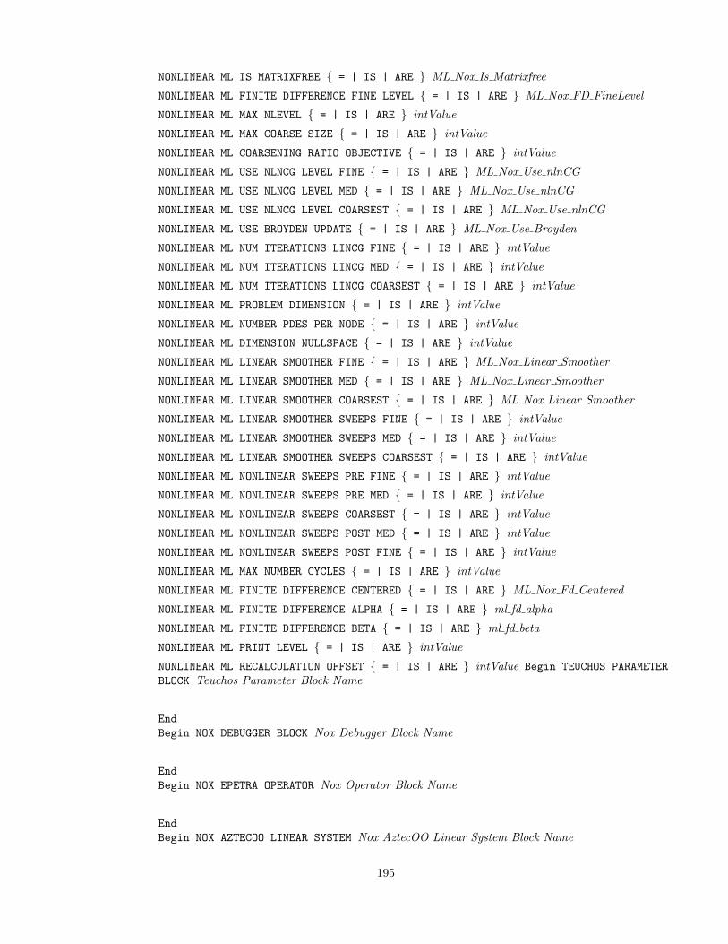
NONLINEAR ML IS MATRIXFREE = | IS | ARE ML Nox Is Matrixfree
NONLINEAR ML FINITE DIFFERENCE FINE LEVEL = | IS | ARE ML Nox FD FineLevel
NONLINEAR ML MAX NLEVEL = | IS | ARE intValue
NONLINEAR ML MAX COARSE SIZE = | IS | ARE intValue
NONLINEAR ML COARSENING RATIO OBJECTIVE = | IS | ARE intValue
NONLINEAR ML USE NLNCG LEVEL FINE = | IS | ARE ML Nox Use nlnCG
NONLINEAR ML USE NLNCG LEVEL MED = | IS | ARE ML Nox Use nlnCG
NONLINEAR ML USE NLNCG LEVEL COARSEST = | IS | ARE ML Nox Use nlnCG
NONLINEAR ML USE BROYDEN UPDATE = | IS | ARE ML Nox Use Broyden
NONLINEAR ML NUM ITERATIONS LINCG FINE = | IS | ARE intValue
NONLINEAR ML NUM ITERATIONS LINCG MED = | IS | ARE intValue
NONLINEAR ML NUM ITERATIONS LINCG COARSEST = | IS | ARE intValue
NONLINEAR ML PROBLEM DIMENSION = | IS | ARE intValue
NONLINEAR ML NUMBER PDES PER NODE = | IS | ARE intValue
NONLINEAR ML DIMENSION NULLSPACE = | IS | ARE intValue
NONLINEAR ML LINEAR SMOOTHER FINE = | IS | ARE ML Nox Linear Smoother
NONLINEAR ML LINEAR SMOOTHER MED = | IS | ARE ML Nox Linear Smoother
NONLINEAR ML LINEAR SMOOTHER COARSEST = | IS | ARE ML Nox Linear Smoother
NONLINEAR ML LINEAR SMOOTHER SWEEPS FINE = | IS | ARE intValue
NONLINEAR ML LINEAR SMOOTHER SWEEPS MED = | IS | ARE intValue
NONLINEAR ML LINEAR SMOOTHER SWEEPS COARSEST = | IS | ARE intValue
NONLINEAR ML NONLINEAR SWEEPS PRE FINE = | IS | ARE intValue
NONLINEAR ML NONLINEAR SWEEPS PRE MED = | IS | ARE intValue
NONLINEAR ML NONLINEAR SWEEPS COARSEST = | IS | ARE intValue
NONLINEAR ML NONLINEAR SWEEPS POST MED = | IS | ARE intValue
NONLINEAR ML NONLINEAR SWEEPS POST FINE = | IS | ARE intValue
NONLINEAR ML MAX NUMBER CYCLES = | IS | ARE intValue
NONLINEAR ML FINITE DIFFERENCE CENTERED = | IS | ARE ML Nox Fd Centered
NONLINEAR ML FINITE DIFFERENCE ALPHA = | IS | ARE ml fd alpha
NONLINEAR ML FINITE DIFFERENCE BETA = | IS | ARE ml fd beta
NONLINEAR ML PRINT LEVEL = | IS | ARE intValue
NONLINEAR ML RECALCULATION OFFSET = | IS | ARE intValue Begin TEUCHOS PARAMETERBLOCK Teuchos Parameter Block Name
EndBegin NOX DEBUGGER BLOCK Nox Debugger Block Name
EndBegin NOX EPETRA OPERATOR Nox Operator Block Name
EndBegin NOX AZTECOO LINEAR SYSTEM Nox AztecOO Linear System Block Name
195
EndBegin NOX LINESEARCH BLOCK Nox Linesearch Block Name
End
End
Details A set of solver parameters for the NOX nonlinear equation solver.
15.1.1 SOLUTION METHOD
Syntax SOLUTION METHOD = | IS | ARE NoxAztecSolverMethods
NoxAztecSolverMethods : no description cg | cgs | bicgstab | gmres| tfqmr | lu
Details Selection of the AztecOO linear solution method.
Enums NoxAztecSolverMethods
cg - no description
cgs - no description
bicgstab - no description
gmres - no description
tfqmr - no description
lu - no description
15.1.2 PRECONDITIONING METHOD
Syntax PRECONDITIONING METHOD = | IS | ARE NoxAztecPreconditionerMethods
NoxAztecPreconditionerMethods : no description none | jacobi| neumann | least-squares | dd-ilut | dd-ilu | user suppliedoperator
Details Selection of the AztecOO preconditioning methods supported by the NOX nonlinearsolver.
196
Enums NoxAztecPreconditionerMethods
none - no description
jacobi - no description
neumann - no description
least-squares - no description
dd-ilut - no description
dd-ilu - no description
user supplied operator - no description
15.1.3 NONLINEAR SOLVER METHOD
Syntax NONLINEAR SOLVER METHOD = | IS | ARE NoxSolverMethods
NoxSolverMethods : no description line search based
Details Selection of the solution method for nonlinear solver.
Enums NoxSolverMethods
line search based - no description
15.1.4 NONLINEAR DIRECTION METHOD
Syntax NONLINEAR DIRECTION METHOD = | IS | ARE NoxDirectionMethods
NoxDirectionMethods : no description newton | nonlinear cg |modified newton | semi-implicit
Details Selection of the direction method to use with a line search based nonlinear solutionmethod.
Enums NoxDirectionMethods
newton - no description
nonlinear cg - no description
modified newton - no description
semi-implicit - no description
197
15.1.5 NONLINEAR JACOBIAN OPERATOR
Syntax NONLINEAR JACOBIAN OPERATOR = | IS | ARE NoxJacobianOperators [allowing diagonal correction ]
NoxJacobianOperators : no description matrix free | finitedifference | finite coloring | user supplied matrix | usersupplied operator
Details Selection of the jacobian operator type
Enums NoxJacobianOperators
matrix free - no description
finite difference - no description
finite coloring - no description
user supplied matrix - no description
user supplied operator - no description
15.1.6 NONLINEAR LINESEARCH METHOD
Syntax NONLINEAR LINESEARCH METHOD = | IS | ARE NoxLinesearchMethods
NoxLinesearchMethods : no description full step | polynomial |quadratic | more thunte | nonlinear cg
Details Selection of the linesearch method for nonlinear solver.
Enums NoxLinesearchMethods
full step - no description
polynomial - no description
quadratic - no description
more thunte - no description
nonlinear cg - no description
15.1.7 NOX NONLINEAR PRECONDITIONING METHOD
Syntax NOX NONLINEAR PRECONDITIONING METHOD = | IS | ARE NoxPreconditioner-Operators [ allowing diagonal correction ]
NoxPreconditionerOperators : no description none | use jacobian |finite difference | finite coloring | user supplied matrix | usersupplied operator | ml
198
Details Selection of NOX nonlinear solver’s preconditioning method.
Enums NoxPreconditionerOperators
none - no description
use jacobian - no description
finite difference - no description
finite coloring - no description
user supplied matrix - no description
user supplied operator - no description
ml - no description
15.1.8 NONLINEAR PRECONDITIONING COMPUTE FREQUENCY
Syntax NONLINEAR PRECONDITIONING COMPUTE FREQUENCY = | IS | ARE frequency
frequency : no description (I)
Details Recompute frequency of the nonlinear preconditioner operator.
15.1.9 RESET COUNTER EACH TIME STEP
Details *** This option is currently inactive. ***
15.1.10 MAX AGE OF JACOBIAN
Syntax MAX AGE OF JACOBIAN = | IS | ARE max age
max age : no description (I)
Details Integer number of nonlinear iterations between recomputations of the Jacobian
15.1.11 FORCING TERM METHOD
Syntax FORCING TERM METHOD = | IS | ARE NoxNewtonSolveOptions
NoxNewtonSolveOptions : no description Constant | Type 1 | Type2
Details Specification of linear solver adaptive forcing term method.
199
Enums NoxNewtonSolveOptions
Constant - no description
Type 1 - no description
Type 2 - no description
15.1.12 FORCING TERM INITIAL TOLERANCE
Syntax FORCING TERM INITIAL TOLERANCE = | IS | ARE init tol
init tol : no description (R)
Details Linear solver adaptive forcing term initial linear solve tolerance.
15.1.13 FORCING TERM MINIMUM TOLERANCE
Syntax FORCING TERM MINIMUM TOLERANCE = | IS | ARE min tol
min tol : no description (R)
Details Linear solver adaptive forcing term minimum linear solve tolerance.
15.1.14 FORCING TERM MAXIMUM TOLERANCE
Syntax FORCING TERM MAXIMUM TOLERANCE = | IS | ARE max tol
max tol : no description (R)
Details Linear solver adaptive forcing term maximum linear solve tolerance.
15.1.15 TYPE 2 FORCING TERM ALPHA
Syntax TYPE 2 FORCING TERM ALPHA = | IS | ARE alpha
alpha : no description (R)
Details Linear solver adaptive forcing term Type 2 value for α
15.1.16 TYPE 2 FORCING TERM GAMMA
Syntax TYPE 2 FORCING TERM GAMMA = | IS | ARE beta
beta : no description (R)
200
Details Linear solver adaptive forcing term Type 2 value for γ
15.1.17 MAXIMUM ITERATIONS
Syntax MAXIMUM ITERATIONS = | IS | ARE max iters
max iters : no description (I)
Details Maximum number of solution method iterations.
15.1.18 RESIDUAL NORM TOLERANCE
Syntax RESIDUAL NORM TOLERANCE = | IS | ARE tol
tol : no description (R)
Details Iterative solution method residual convergence tolerance.
15.1.19 RESTART ITERATIONS
Syntax RESTART ITERATIONS = | IS | ARE restart iters
restart iters : no description (I)
Details Number of iterations between GMRES restarts.
15.1.20 PRECONDITIONING STEPS
Syntax PRECONDITIONING STEPS = | IS | ARE steps
steps : no description (I)
Details Number of Jacobi, Gauss-Seidel, or other preconditioning methods’ applications periteration.
15.1.21 POLYNOMIAL ORDER
Syntax POLYNOMIAL ORDER = | IS | ARE order
order : no description (I)
Details Polynomial order of preconditioning method.
201
15.1.22 MAXIMUM NONLINEAR ITERATIONS
Syntax MAXIMUM NONLINEAR ITERATIONS = | IS | ARE max iters
max iters : no description (I)
Details Maximum number of nonlinear solver iterations.
15.1.23 NONLINEAR ABSOLUTE RESIDUAL NORM TOLERANCE
Syntax NONLINEAR ABSOLUTE RESIDUAL NORM TOLERANCE = | IS | ARE abs res tol
abs res tol : no description (R)
Details Nonlinear absolute residual norm convergence tolerance.
15.1.24 NONLINEAR RELATIVE RESIDUAL NORM TOLERANCE
Syntax NONLINEAR RELATIVE RESIDUAL NORM TOLERANCE = | IS | ARE rel res tol
rel res tol : no description (R)
Details Nonlinear relative residual convergence tolerance.
15.1.25 ILL CONDITIONING THRESHOLD
Syntax ILL CONDITIONING THRESHOLD = | IS | ARE threshold
threshold : no description (R)
Details Ill-conditioning threshold for linear solver
15.1.26 ILU OVERLAP
Syntax ILU OVERLAP = | IS | ARE overlap
overlap : no description (I)
Details Overlap parameter for incomplete factorizations.
202
15.1.27 ILU GRAPH FILL
Syntax ILU GRAPH FILL = | IS | ARE fill
fill : no description (I)
Details Graph fill factor for incomplete factorizations.
15.1.28 ILUT FILL FACTOR
Syntax ILUT FILL FACTOR = | IS | ARE fill factor
fill factor : no description (R)
Details Fill factor for incomplete threshold factorizations.
15.1.29 ILUT DROP TOLERANCE
Syntax ILUT DROP TOLERANCE = | IS | ARE tolerance
tolerance : no description (R)
Details Drop tolerance for incomplete threshold factorizations.
15.1.30 PRECONDITIONING PACKAGE
Syntax PRECONDITIONING PACKAGE = | IS | ARE PreconditioningPackages [ usingTeuchos Param List Name ]
PreconditioningPackages : no description aztecoo | ifpack |multilevel
Teuchos Param List Name : no description (C)
Details Specify which package to use for preconditioning.
Enums PreconditioningPackages
aztecoo - no description
ifpack - no description
multilevel - no description
203
15.1.31 MATRIX FREE FINITE DIFFERENCE METHOD
Syntax MATRIX FREE FINITE DIFFERENCE METHOD = | IS | ARE NoxDifferencin-gOptions
NoxDifferencingOptions : no description forward difference |backward difference | centered difference
Details Finite differencing method used for matrix-free.
Enums NoxDifferencingOptions
forward difference - no description
backward difference - no description
centered difference - no description
15.1.32 FINITE DIFFERENCE METHOD
Syntax FINITE DIFFERENCE METHOD = | IS | ARE NoxDifferencingOptions
NoxDifferencingOptions : no description forward difference |backward difference | centered difference
Details Finite differencing method.
Enums NoxDifferencingOptions
forward difference - no description
backward difference - no description
centered difference - no description
15.1.33 PERTURBATION COEFFICIENT ALPHA
Syntax PERTURBATION COEFFICIENT ALPHA = | IS | ARE FDalpha
FDalpha : no description (R)
Details Parameter, α, used in finite differencing perturbation value calculation.
15.1.34 PERTURBATION COEFFICIENT BETA
Syntax PERTURBATION COEFFICIENT BETA = | IS | ARE FDbeta
FDbeta : no description (R)
204
Details Parameter, β, used in finite differencing perturbation value calculation.
15.1.35 MATRIX FREE PERTURBATION COEFFICIENT LAMBDA
Syntax MATRIX FREE PERTURBATION COEFFICIENT LAMBDA = | IS | ARE MFlambda
MFlambda : no description (R)
Details Parameter, lambda, used to compute the perturbation size used in matrix-free resid-ual evaluations.
15.1.36 MATRIX FREE PERTURBATION COEFFICIENT VALUE
Syntax MATRIX FREE PERTURBATION COEFFICIENT VALUE = | IS | ARE MFepsilon
MFepsilon : no description (R)
Details Direct specification for pertuebation size used in matrix-free residual evaluations.
15.1.37 RESCUE BAD NEWTON SOLVE
Details Flag to specify if an unconverged linear solve solution should be accepted or flaggedas failed.
15.1.38 USE RCM REORDERING
Details Flag to specify whether or not to reorder the matrix via the Reverse Cuthill-McGeealgorithm.
15.1.39 DISTINGUISH MATRIX FREE FILLS
Details Flag to specify whether or not to treat Matrix-Free residual fills different than fillsused as the right-hand-side in Newton methods.
15.1.40 STAGNATION TEST TOLERANCE
Syntax STAGNATION TEST TOLERANCE = | IS | ARE stag test tol
stag test tol : no description (R)
Details Maximum allowed ratio of nonlinear residuals used to define stagnation event.
205
15.1.41 STAGNATION TEST STEPS
Syntax STAGNATION TEST STEPS = | IS | ARE stag test steps
stag test steps : no description (I)
Details Maximum number of consecutive nonlinear iterations that the residual ratio is allowedto be above its maximum value.
15.1.42 LINEAR STAGNATION TEST TOLERANCE
Syntax LINEAR STAGNATION TEST TOLERANCE = | IS | ARE lin stag test tol
lin stag test tol : no description (R)
Details Maximum allowed ratio of linear residuals used to define stagnation event.
15.1.43 LINEAR STAGNATION TEST STEPS
Syntax LINEAR STAGNATION TEST STEPS = | IS | ARE lin stag test steps
lin stag test steps : no description (I)
Details Maximum number of consecutive linear iterations that the linear residual ratio isallowed to be above its maximum value.
15.1.44 NONLINEAR ABSOLUTE UPDATE NORM TOLERANCE
Syntax NONLINEAR ABSOLUTE UPDATE NORM TOLERANCE = | IS | ARE abs update tol
abs update tol : no description (R)
Details Absolute update norm convergence tolerance.
15.1.45 USER DEFINED CONVERGENCE
Details Flag to specify whether or not to allow the application to defined convergence.
15.1.46 MINIMUM NONLINEAR ITERATIONS
Syntax MINIMUM NONLINEAR ITERATIONS = | IS | ARE req min nonlin iters
req min nonlin iters : no description (I)
206
Details Specifies a required minimum number of nonlinear iterations.
15.1.47 LINEAR SOLVER OUTPUT FREQUENCY
Syntax LINEAR SOLVER OUTPUT FREQUENCY = | IS | ARE lin output freq
lin output freq : no description (I)
Details Output frequency for iterative linear solvers.
15.1.48 COLORING ALGORITHM
Syntax COLORING ALGORITHM = | IS | ARE NoxColoringMethods
NoxColoringMethods : no description greedy | luby
Details Specify which coloring algorithm to use.
Enums NoxColoringMethods
greedy - no description
luby - no description
15.1.49 COLORING REORDERING
Syntax COLORING REORDERING = | IS | ARE NoxColoringReordering
NoxColoringReordering : no description largest first | smallestfirst | random
Details Specify how to reorder during coloring.
Enums NoxColoringReordering
largest first - no description
smallest first - no description
random - no description
15.1.50 COLOR GRAPH USING DISTANCE1
Details Flag indicating use of distance1 coloring of matrix graph.
207
15.1.51 DUMP JACOBIAN MATRIX
Syntax DUMP JACOBIAN MATRIX to MatrixOutputFormat
MatrixOutputFormat : no description ascii | matrix market
Details Debugging flag to allow the user to print the Jacobian matrix and then exit.
Enums MatrixOutputFormat
ascii - no description
matrix market - no description
15.1.52 DUMP RESIDUAL VECTOR
Syntax DUMP RESIDUAL VECTOR to MatrixOutputFormat
MatrixOutputFormat : no description ascii | matrix market
Details Debugging flag to allow the user to print the Residual vector and then exit.
Enums MatrixOutputFormat
ascii - no description
matrix market - no description
15.1.53 DUMP INITIAL GUESS VECTOR
Syntax DUMP INITIAL GUESS VECTOR to MatrixOutputFormat
MatrixOutputFormat : no description ascii | matrix market
Details Debugging flag to allow the user to print the initial guess for the nonlinear solutionand then exit.
Enums MatrixOutputFormat
ascii - no description
matrix market - no description
15.1.54 DUMP LINEAR SOLUTION VECTOR
Syntax DUMP LINEAR SOLUTION VECTOR to MatrixOutputFormat
MatrixOutputFormat : no description ascii | matrix market
208
Details Debugging flag to allow the user to first compute and then dump the vector obtainedfrom doing a linear solve at the current nonlinear iteration and then exit.
Enums MatrixOutputFormat
ascii - no description
matrix market - no description
15.1.55 OUTPUT NONLINEAR OBJECTS
Syntax OUTPUT NONLINEAR OBJECTS using param list name
param list name : no description (C)
Details Specify nonlinear solver object output using a named teuchos parameter list.
15.1.56 SETUP NONLINEAR SOLVER
Syntax SETUP NONLINEAR SOLVER using setup params list name
setup params list name : no description (C)
Details Specify options to use when setting up the nonlinear solver.
15.1.57 NOX OUTPUT LEVEL
Syntax NOX OUTPUT LEVEL = | IS | ARE NoxOutputLevels
NoxOutputLevels : no description low | medium | high
Details Level specification for amount of output from the NOX nonlinear solver
Enums NoxOutputLevels
low - no description
medium - no description
high - no description
15.1.58 NOX OUTPUT VALUE
Syntax NOX OUTPUT VALUE = | IS | ARE intValue
intValue : no description (I)
209
Details Integer specification for amount of output from the NOX nonlinear solver. Valuesrange from 0-256.
15.1.59 USE NOX OPERATOR DEBUGGER
Syntax USE NOX OPERATOR DEBUGGER = | IS | ARE Debugger Name
Debugger Name : no description (C)
Details Specifies which NOX operator (e.g. Jacobian) debugger to use.
15.1.60 USE NOX LINEAR SYSTEM
Syntax USE NOX LINEAR SYSTEM = | IS | ARE Linear System Name
Linear System Name : no description (C)
Details Specifies which NOX Linear System to use.
15.1.61 USE NOX LINESEARCH
Syntax USE NOX LINESEARCH = | IS | ARE Linesearch Name
Linesearch Name : no description (C)
Details Specifies which NOX Linesearch to use.
15.1.62 NONLINEAR ML COARSENING METHOD
Details Choose ML coarsening method.
15.1.63 NONLINEAR ML IS LINEAR PRECONDITIONER
Details Choose ML to act as non-/linear preconditioner.
15.1.64 NONLINEAR ML IS MATRIXFREE
Details Choose ML to be matrixfree preconditioner.
210
15.1.65 NONLINEAR ML FINITE DIFFERENCE FINE LEVEL
Details Choose ML to construct fine level full Jacobian.
15.1.66 NONLINEAR ML MAX NLEVEL
Syntax NONLINEAR ML MAX NLEVEL = | IS | ARE intValue
intValue : no description (I)
Details Integer maximum number of levels.
15.1.67 NONLINEAR ML MAX COARSE SIZE
Syntax NONLINEAR ML MAX COARSE SIZE = | IS | ARE intValue
intValue : no description (I)
Details Size of coarse grid where to stop coarsening further.
15.1.68 NONLINEAR ML COARSENING RATIO OBJECTIVE
Syntax NONLINEAR ML COARSENING RATIO OBJECTIVE = | IS | ARE intValue
intValue : no description (I)
Details Coarsening ratio objective.
15.1.69 NONLINEAR ML USE NLNCG LEVEL FINE
Details Choose ML to use nlnCG on fine level.
15.1.70 NONLINEAR ML USE NLNCG LEVEL MED
Details Choose ML to use nlnCG on all medium levels.
15.1.71 NONLINEAR ML USE NLNCG LEVEL COARSEST
Details Choose ML to use nlnCG on coarsest level.
211

15.1.72 NONLINEAR ML USE BROYDEN UPDATE
Details Choose ML to use a Broyden update on all levels that use Newton’s method.
15.1.73 NONLINEAR ML NUM ITERATIONS LINCG FINE
Syntax NONLINEAR ML NUM ITERATIONS LINCG FINE = | IS | ARE intValue
intValue : no description (I)
Details Number of linear CG iterations in Newton step on level fine.
15.1.74 NONLINEAR ML NUM ITERATIONS LINCG MED
Syntax NONLINEAR ML NUM ITERATIONS LINCG MED = | IS | ARE intValue
intValue : no description (I)
Details Number of linear CG iterations in Newton step on level med.
15.1.75 NONLINEAR ML NUM ITERATIONS LINCG COARSEST
Syntax NONLINEAR ML NUM ITERATIONS LINCG COARSEST = | IS | ARE intValue
intValue : no description (I)
Details Number of linear CG iterations in Newton step on level coarsest.
15.1.76 NONLINEAR ML PROBLEM DIMENSION
Syntax NONLINEAR ML PROBLEM DIMENSION = | IS | ARE intValue
intValue : no description (I)
Details Dimension of the problem (3D, 2D, 1D).
15.1.77 NONLINEAR ML NUMBER PDES PER NODE
Syntax NONLINEAR ML NUMBER PDES PER NODE = | IS | ARE intValue
intValue : no description (I)
212
Details Number of PDEs (dofs) per node.
15.1.78 NONLINEAR ML DIMENSION NULLSPACE
Syntax NONLINEAR ML DIMENSION NULLSPACE = | IS | ARE intValue
intValue : no description (I)
Details Dimension of the Nullspace of the problem (6 in 3D, 3 in 2D, 1 in 1D).
15.1.79 NONLINEAR ML LINEAR SMOOTHER FINE
Details Choose ML linear smoother.
15.1.80 NONLINEAR ML LINEAR SMOOTHER MED
Details Choose ML linear smoother.
15.1.81 NONLINEAR ML LINEAR SMOOTHER COARSEST
Details Choose ML linear smoother.
15.1.82 NONLINEAR ML LINEAR SMOOTHER SWEEPS FINE
Syntax NONLINEAR ML LINEAR SMOOTHER SWEEPS FINE = | IS | ARE intValue
intValue : no description (I)
Details Number of sweeps of linear smoother.
15.1.83 NONLINEAR ML LINEAR SMOOTHER SWEEPS MED
Syntax NONLINEAR ML LINEAR SMOOTHER SWEEPS MED = | IS | ARE intValue
intValue : no description (I)
Details Number of sweeps of linear smoother.
213
15.1.84 NONLINEAR ML LINEAR SMOOTHER SWEEPS COARS-EST
Syntax NONLINEAR ML LINEAR SMOOTHER SWEEPS COARSEST = | IS | ARE intValue
intValue : no description (I)
Details Number of sweeps of linear smoother.
15.1.85 NONLINEAR ML NONLINEAR SWEEPS PRE FINE
Syntax NONLINEAR ML NONLINEAR SWEEPS PRE FINE = | IS | ARE intValue
intValue : no description (I)
Details Number of presmooth sweeps of nonlinear smoother fine.
15.1.86 NONLINEAR ML NONLINEAR SWEEPS PRE MED
Syntax NONLINEAR ML NONLINEAR SWEEPS PRE MED = | IS | ARE intValue
intValue : no description (I)
Details Number of presmooth sweeps of nonlinear smoother med.
15.1.87 NONLINEAR ML NONLINEAR SWEEPS COARSEST
Syntax NONLINEAR ML NONLINEAR SWEEPS COARSEST = | IS | ARE intValue
intValue : no description (I)
Details Number of sweeps of nonlinear smoother coarsest.
15.1.88 NONLINEAR ML NONLINEAR SWEEPS POST MED
Syntax NONLINEAR ML NONLINEAR SWEEPS POST MED = | IS | ARE intValue
intValue : no description (I)
Details Number of postsmooth sweeps of nonlinear smoother med.
214
15.1.89 NONLINEAR ML NONLINEAR SWEEPS POST FINE
Syntax NONLINEAR ML NONLINEAR SWEEPS POST FINE = | IS | ARE intValue
intValue : no description (I)
Details Number of postsmooth sweeps of nonlinear smoother fine.
15.1.90 NONLINEAR ML MAX NUMBER CYCLES
Syntax NONLINEAR ML MAX NUMBER CYCLES = | IS | ARE intValue
intValue : no description (I)
Details max Number of cycles for nox ml as a solver.
15.1.91 NONLINEAR ML FINITE DIFFERENCE CENTERED
Details Choose ML finite differencing method.
15.1.92 NONLINEAR ML FINITE DIFFERENCE ALPHA
Syntax NONLINEAR ML FINITE DIFFERENCE ALPHA = | IS | ARE ml fd alpha
ml fd alpha : no description (R)
Details Finite Differencing perturbation parameter alpha.
15.1.93 NONLINEAR ML FINITE DIFFERENCE BETA
Syntax NONLINEAR ML FINITE DIFFERENCE BETA = | IS | ARE ml fd beta
ml fd beta : no description (R)
Details Finite Differencing perturbation parameter alpha.
15.1.94 NONLINEAR ML PRINT LEVEL
Syntax NONLINEAR ML PRINT LEVEL = | IS | ARE intValue
intValue : no description (I)
215
Details Output level (0-10).
15.1.95 NONLINEAR ML RECALCULATION OFFSET
Syntax NONLINEAR ML RECALCULATION OFFSET = | IS | ARE intValue
intValue : no description (I)
Details Recalculation of preconditioner offset.
15.2 TEUCHOS PARAMETER BLOCK
Begin TEUCHOS PARAMETER BLOCK Teuchos Parameter Block Name
PARAM-STRING parameter name VALUE string value
PARAM-REAL parameter name VALUE real value
PARAM-INT parameter name VALUE integer value
PARAM-BOOL parameter name VALUE false | true PARAM-SUBLIST parameter name VALUE block name
End
Details A block to set a Teuchos parameter list.
15.2.1 PARAM-STRING
Syntax PARAM-STRING parameter name VALUE string value
parameter name : no description (Q)
string value : no description (Q)
Details Key/Value string-pair to be passed to solver.
15.2.2 PARAM-REAL
Syntax PARAM-REAL parameter name VALUE real value
parameter name : no description (Q)
real value : no description (R)
216
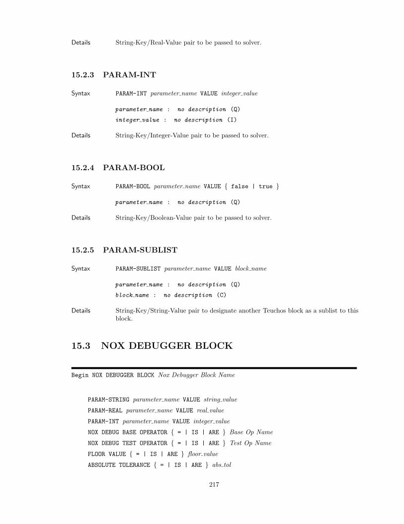
Details String-Key/Real-Value pair to be passed to solver.
15.2.3 PARAM-INT
Syntax PARAM-INT parameter name VALUE integer value
parameter name : no description (Q)
integer value : no description (I)
Details String-Key/Integer-Value pair to be passed to solver.
15.2.4 PARAM-BOOL
Syntax PARAM-BOOL parameter name VALUE false | true
parameter name : no description (Q)
Details String-Key/Boolean-Value pair to be passed to solver.
15.2.5 PARAM-SUBLIST
Syntax PARAM-SUBLIST parameter name VALUE block name
parameter name : no description (Q)
block name : no description (C)
Details String-Key/String-Value pair to designate another Teuchos block as a sublist to thisblock.
15.3 NOX DEBUGGER BLOCK
Begin NOX DEBUGGER BLOCK Nox Debugger Block Name
PARAM-STRING parameter name VALUE string value
PARAM-REAL parameter name VALUE real value
PARAM-INT parameter name VALUE integer value
NOX DEBUG BASE OPERATOR = | IS | ARE Base Op Name
NOX DEBUG TEST OPERATOR = | IS | ARE Test Op Name
FLOOR VALUE = | IS | ARE floor value
ABSOLUTE TOLERANCE = | IS | ARE abs tol
217
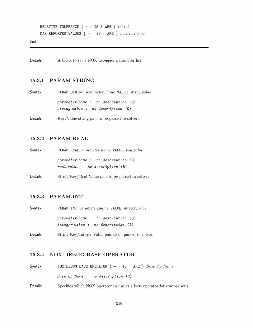
RELATIVE TOLERANCE = | IS | ARE rel tol
MAX REPORTED VALUES = | IS | ARE max to report
End
Details A block to set a NOX debugger parameter list.
15.3.1 PARAM-STRING
Syntax PARAM-STRING parameter name VALUE string value
parameter name : no description (Q)
string value : no description (Q)
Details Key/Value string-pair to be passed to solver.
15.3.2 PARAM-REAL
Syntax PARAM-REAL parameter name VALUE real value
parameter name : no description (Q)
real value : no description (R)
Details String-Key/Real-Value pair to be passed to solver.
15.3.3 PARAM-INT
Syntax PARAM-INT parameter name VALUE integer value
parameter name : no description (Q)
integer value : no description (I)
Details String-Key/Integer-Value pair to be passed to solver.
15.3.4 NOX DEBUG BASE OPERATOR
Syntax NOX DEBUG BASE OPERATOR = | IS | ARE Base Op Name
Base Op Name : no description (C)
Details Specifies which NOX operator to use as a base operator for comparisons.
218
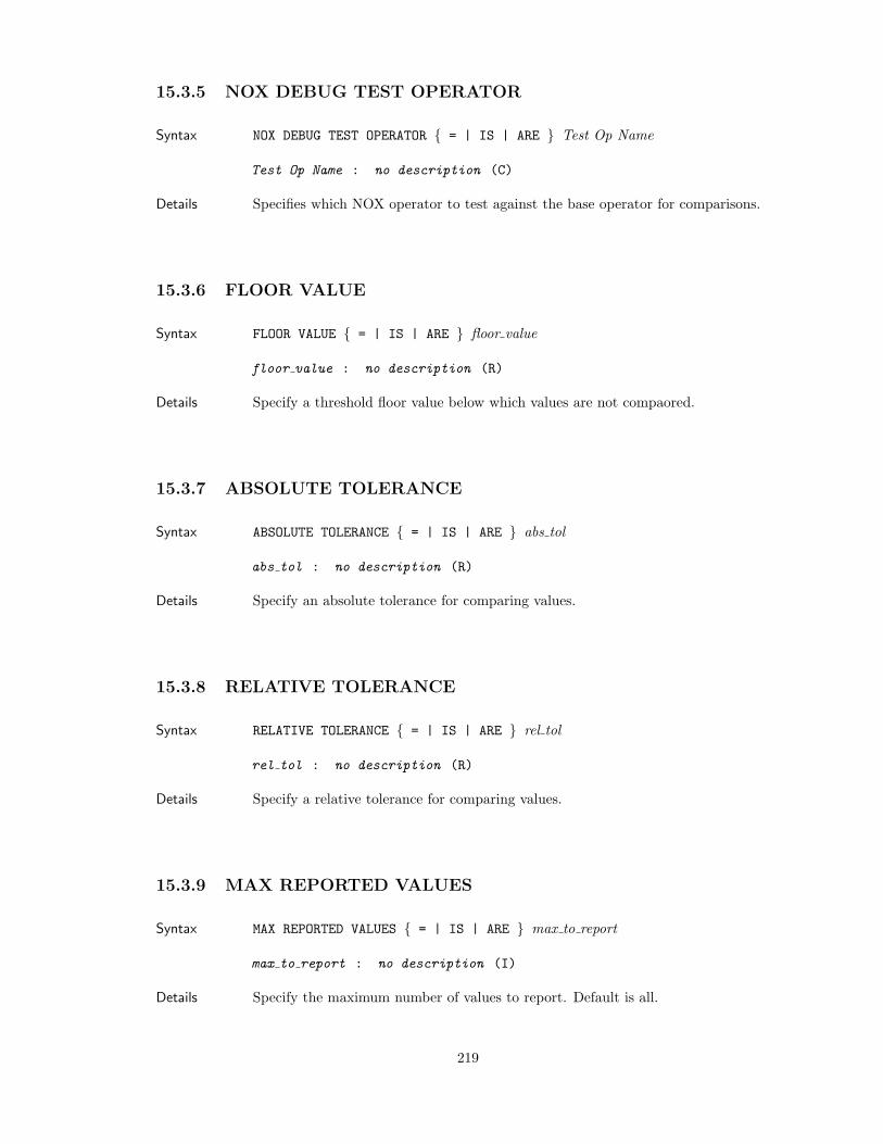
15.3.5 NOX DEBUG TEST OPERATOR
Syntax NOX DEBUG TEST OPERATOR = | IS | ARE Test Op Name
Test Op Name : no description (C)
Details Specifies which NOX operator to test against the base operator for comparisons.
15.3.6 FLOOR VALUE
Syntax FLOOR VALUE = | IS | ARE floor value
floor value : no description (R)
Details Specify a threshold floor value below which values are not compaored.
15.3.7 ABSOLUTE TOLERANCE
Syntax ABSOLUTE TOLERANCE = | IS | ARE abs tol
abs tol : no description (R)
Details Specify an absolute tolerance for comparing values.
15.3.8 RELATIVE TOLERANCE
Syntax RELATIVE TOLERANCE = | IS | ARE rel tol
rel tol : no description (R)
Details Specify a relative tolerance for comparing values.
15.3.9 MAX REPORTED VALUES
Syntax MAX REPORTED VALUES = | IS | ARE max to report
max to report : no description (I)
Details Specify the maximum number of values to report. Default is all.
219
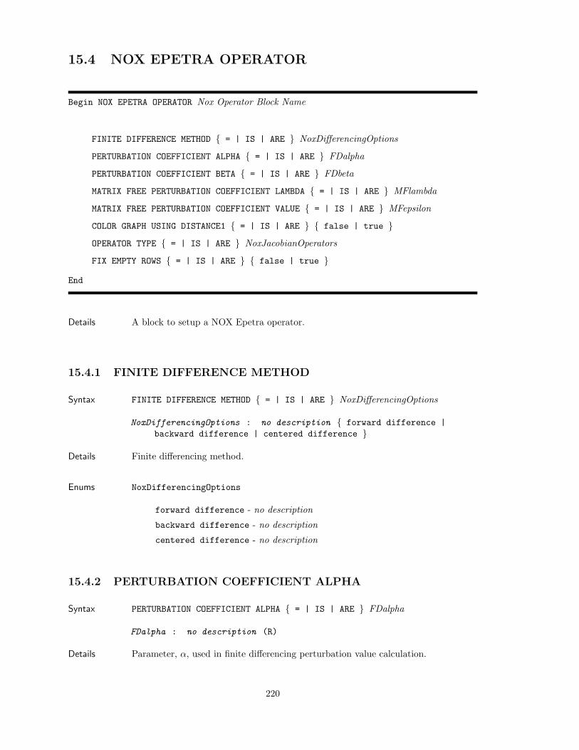
15.4 NOX EPETRA OPERATOR
Begin NOX EPETRA OPERATOR Nox Operator Block Name
FINITE DIFFERENCE METHOD = | IS | ARE NoxDifferencingOptions
PERTURBATION COEFFICIENT ALPHA = | IS | ARE FDalpha
PERTURBATION COEFFICIENT BETA = | IS | ARE FDbeta
MATRIX FREE PERTURBATION COEFFICIENT LAMBDA = | IS | ARE MFlambda
MATRIX FREE PERTURBATION COEFFICIENT VALUE = | IS | ARE MFepsilon
COLOR GRAPH USING DISTANCE1 = | IS | ARE false | true
OPERATOR TYPE = | IS | ARE NoxJacobianOperators
FIX EMPTY ROWS = | IS | ARE false | true
End
Details A block to setup a NOX Epetra operator.
15.4.1 FINITE DIFFERENCE METHOD
Syntax FINITE DIFFERENCE METHOD = | IS | ARE NoxDifferencingOptions
NoxDifferencingOptions : no description forward difference |backward difference | centered difference
Details Finite differencing method.
Enums NoxDifferencingOptions
forward difference - no description
backward difference - no description
centered difference - no description
15.4.2 PERTURBATION COEFFICIENT ALPHA
Syntax PERTURBATION COEFFICIENT ALPHA = | IS | ARE FDalpha
FDalpha : no description (R)
Details Parameter, α, used in finite differencing perturbation value calculation.
220
15.4.3 PERTURBATION COEFFICIENT BETA
Syntax PERTURBATION COEFFICIENT BETA = | IS | ARE FDbeta
FDbeta : no description (R)
Details Parameter, β, used in finite differencing perturbation value calculation.
15.4.4 MATRIX FREE PERTURBATION COEFFICIENT LAMBDA
Syntax MATRIX FREE PERTURBATION COEFFICIENT LAMBDA = | IS | ARE MFlambda
MFlambda : no description (R)
Details Parameter, lambda, used to compute the perturbation size used in matrix-free resid-ual evaluations.
15.4.5 MATRIX FREE PERTURBATION COEFFICIENT VALUE
Syntax MATRIX FREE PERTURBATION COEFFICIENT VALUE = | IS | ARE MFepsilon
MFepsilon : no description (R)
Details Direct specification for pertuebation size used in matrix-free residual evaluations.
15.4.6 COLOR GRAPH USING DISTANCE1
Details Flag indicating use of distance1 coloring of matrix graph.
15.4.7 OPERATOR TYPE
Syntax OPERATOR TYPE = | IS | ARE NoxJacobianOperators
NoxJacobianOperators : no description matrix free | finitedifference | finite coloring | user supplied matrix | usersupplied operator
Details Selection of the operator type
221
Enums NoxJacobianOperators
matrix free - no description
finite difference - no description
finite coloring - no description
user supplied matrix - no description
user supplied operator - no description
15.4.8 FIX EMPTY ROWS
Details Flag whether or not to correct empty matrix rows
15.5 NOX AZTECOO LINEAR SYSTEM
Begin NOX AZTECOO LINEAR SYSTEM Nox AztecOO Linear System Block Name
SOLUTION METHOD = | IS | ARE NoxAztecSolverMethods
LINEAR SYSTEM TYPE = | IS | ARE NoxLinearSystemTypes
PRECONDITIONING METHOD = | IS | ARE NoxAztecPreconditionerMethods
PRECONDITION USING JACOBIAN = | IS | ARE false | true
NONLINEAR PRECONDITIONING COMPUTE FREQUENCY = | IS | ARE frequency
MAX AGE OF JACOBIAN = | IS | ARE max age
FORCING TERM METHOD = | IS | ARE NoxNewtonSolveOptions
FORCING TERM INITIAL TOLERANCE = | IS | ARE init tol
FORCING TERM MINIMUM TOLERANCE = | IS | ARE min tol
FORCING TERM MAXIMUM TOLERANCE = | IS | ARE max tol
TYPE 2 FORCING TERM ALPHA = | IS | ARE alpha
TYPE 2 FORCING TERM GAMMA = | IS | ARE beta
MAXIMUM ITERATIONS = | IS | ARE max iters
RESIDUAL NORM TOLERANCE = | IS | ARE tol
RESTART ITERATIONS = | IS | ARE restart iters
PRECONDITIONING PACKAGE = | IS | ARE PreconditioningPackages [ using Teuchos Param List Name]
RESCUE BAD NEWTON SOLVE = | IS | ARE false | true
LINEAR SOLVER OUTPUT FREQUENCY = | IS | ARE lin output freq
SET JACOBIAN OPERATOR = | IS | ARE Operator Name
SET PRECONDITIONER OPERATOR = | IS | ARE Operator Name
222
End
Details A block to setup a NOX AztecOO Linear System.
15.5.1 SOLUTION METHOD
Syntax SOLUTION METHOD = | IS | ARE NoxAztecSolverMethods
NoxAztecSolverMethods : no description cg | cgs | bicgstab | gmres| tfqmr | lu
Details Selection of the AztecOO linear solution method.
Enums NoxAztecSolverMethods
cg - no description
cgs - no description
bicgstab - no description
gmres - no description
tfqmr - no description
lu - no description
15.5.2 LINEAR SYSTEM TYPE
Syntax LINEAR SYSTEM TYPE = | IS | ARE NoxLinearSystemTypes
NoxLinearSystemTypes : no description aztecoo | semi-implicit |belos | generic sierra linear solver
Details Selection of the NOX Linear System type.
Enums NoxLinearSystemTypes
aztecoo - no description
semi-implicit - no description
belos - no description
generic sierra linear solver - no description
223
15.5.3 PRECONDITIONING METHOD
Syntax PRECONDITIONING METHOD = | IS | ARE NoxAztecPreconditionerMethods
NoxAztecPreconditionerMethods : no description none | jacobi| neumann | least-squares | dd-ilut | dd-ilu | user suppliedoperator
Details Selection of the AztecOO preconditioning methods supported by the NOX nonlinearsolver.
Enums NoxAztecPreconditionerMethods
none - no description
jacobi - no description
neumann - no description
least-squares - no description
dd-ilut - no description
dd-ilu - no description
user supplied operator - no description
15.5.4 PRECONDITION USING JACOBIAN
Details Flag whether or not to use tha Jacobian operator as the preconditioner operator
15.5.5 NONLINEAR PRECONDITIONING COMPUTE FREQUENCY
Syntax NONLINEAR PRECONDITIONING COMPUTE FREQUENCY = | IS | ARE frequency
frequency : no description (I)
Details Recompute frequency of the nonlinear preconditioner operator.
15.5.6 MAX AGE OF JACOBIAN
Syntax MAX AGE OF JACOBIAN = | IS | ARE max age
max age : no description (I)
Details Integer number of nonlinear iterations between recomputations of the Jacobian
224
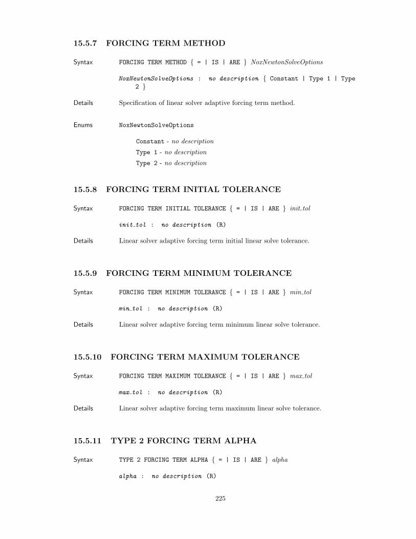
15.5.7 FORCING TERM METHOD
Syntax FORCING TERM METHOD = | IS | ARE NoxNewtonSolveOptions
NoxNewtonSolveOptions : no description Constant | Type 1 | Type2
Details Specification of linear solver adaptive forcing term method.
Enums NoxNewtonSolveOptions
Constant - no description
Type 1 - no description
Type 2 - no description
15.5.8 FORCING TERM INITIAL TOLERANCE
Syntax FORCING TERM INITIAL TOLERANCE = | IS | ARE init tol
init tol : no description (R)
Details Linear solver adaptive forcing term initial linear solve tolerance.
15.5.9 FORCING TERM MINIMUM TOLERANCE
Syntax FORCING TERM MINIMUM TOLERANCE = | IS | ARE min tol
min tol : no description (R)
Details Linear solver adaptive forcing term minimum linear solve tolerance.
15.5.10 FORCING TERM MAXIMUM TOLERANCE
Syntax FORCING TERM MAXIMUM TOLERANCE = | IS | ARE max tol
max tol : no description (R)
Details Linear solver adaptive forcing term maximum linear solve tolerance.
15.5.11 TYPE 2 FORCING TERM ALPHA
Syntax TYPE 2 FORCING TERM ALPHA = | IS | ARE alpha
alpha : no description (R)
225
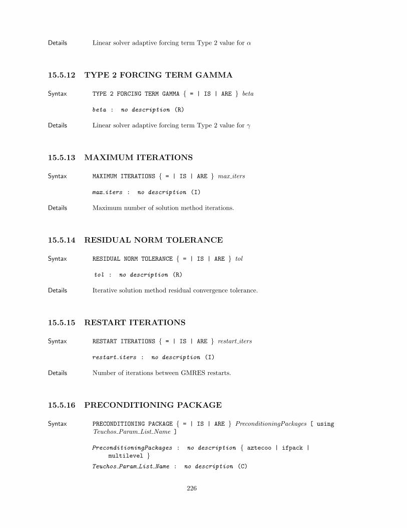
Details Linear solver adaptive forcing term Type 2 value for α
15.5.12 TYPE 2 FORCING TERM GAMMA
Syntax TYPE 2 FORCING TERM GAMMA = | IS | ARE beta
beta : no description (R)
Details Linear solver adaptive forcing term Type 2 value for γ
15.5.13 MAXIMUM ITERATIONS
Syntax MAXIMUM ITERATIONS = | IS | ARE max iters
max iters : no description (I)
Details Maximum number of solution method iterations.
15.5.14 RESIDUAL NORM TOLERANCE
Syntax RESIDUAL NORM TOLERANCE = | IS | ARE tol
tol : no description (R)
Details Iterative solution method residual convergence tolerance.
15.5.15 RESTART ITERATIONS
Syntax RESTART ITERATIONS = | IS | ARE restart iters
restart iters : no description (I)
Details Number of iterations between GMRES restarts.
15.5.16 PRECONDITIONING PACKAGE
Syntax PRECONDITIONING PACKAGE = | IS | ARE PreconditioningPackages [ usingTeuchos Param List Name ]
PreconditioningPackages : no description aztecoo | ifpack |multilevel
Teuchos Param List Name : no description (C)
226
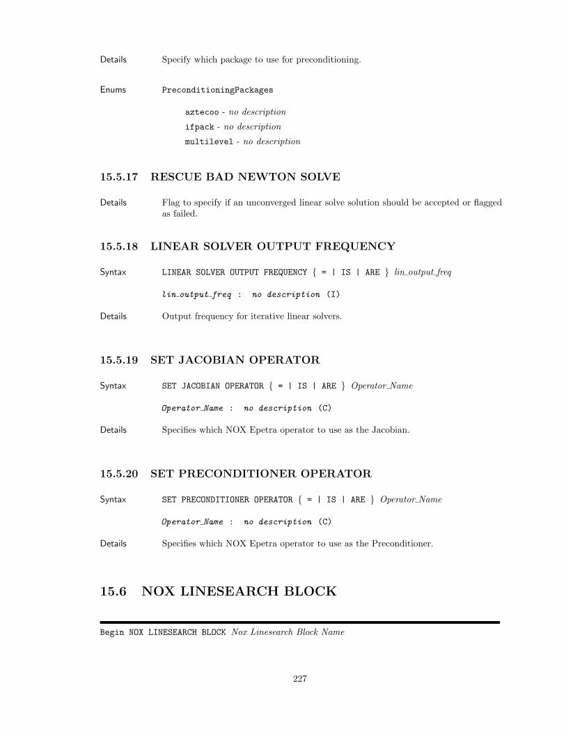
Details Specify which package to use for preconditioning.
Enums PreconditioningPackages
aztecoo - no description
ifpack - no description
multilevel - no description
15.5.17 RESCUE BAD NEWTON SOLVE
Details Flag to specify if an unconverged linear solve solution should be accepted or flaggedas failed.
15.5.18 LINEAR SOLVER OUTPUT FREQUENCY
Syntax LINEAR SOLVER OUTPUT FREQUENCY = | IS | ARE lin output freq
lin output freq : no description (I)
Details Output frequency for iterative linear solvers.
15.5.19 SET JACOBIAN OPERATOR
Syntax SET JACOBIAN OPERATOR = | IS | ARE Operator Name
Operator Name : no description (C)
Details Specifies which NOX Epetra operator to use as the Jacobian.
15.5.20 SET PRECONDITIONER OPERATOR
Syntax SET PRECONDITIONER OPERATOR = | IS | ARE Operator Name
Operator Name : no description (C)
Details Specifies which NOX Epetra operator to use as the Preconditioner.
15.6 NOX LINESEARCH BLOCK
Begin NOX LINESEARCH BLOCK Nox Linesearch Block Name
227
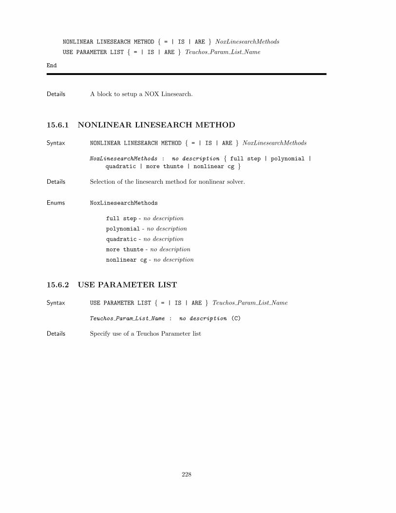
NONLINEAR LINESEARCH METHOD = | IS | ARE NoxLinesearchMethods
USE PARAMETER LIST = | IS | ARE Teuchos Param List Name
End
Details A block to setup a NOX Linesearch.
15.6.1 NONLINEAR LINESEARCH METHOD
Syntax NONLINEAR LINESEARCH METHOD = | IS | ARE NoxLinesearchMethods
NoxLinesearchMethods : no description full step | polynomial |quadratic | more thunte | nonlinear cg
Details Selection of the linesearch method for nonlinear solver.
Enums NoxLinesearchMethods
full step - no description
polynomial - no description
quadratic - no description
more thunte - no description
nonlinear cg - no description
15.6.2 USE PARAMETER LIST
Syntax USE PARAMETER LIST = | IS | ARE Teuchos Param List Name
Teuchos Param List Name : no description (C)
Details Specify use of a Teuchos Parameter list
228
Chapter 16
LOCA Continuation SolverReference
See, also, the LOCA parameters online reference.
16.1 LOCA CONTINUATION SOLVER
Begin LOCA CONTINUATION SOLVER LOCA Solver Name
USE NOX SOLVER = | IS | ARE nox solver name
USE PARAMETER LIST = | IS | ARE param list name Begin TEUCHOS PARAMETER BLOCKTeuchos Parameter Block Name
End
End
Details A set of solver parameters for LOCA continuation solver.
16.1.1 USE NOX SOLVER
Syntax USE NOX SOLVER = | IS | ARE nox solver name
nox solver name : no description (C)
Details Specify a NOX solver to use for the nonlinear solves.
229
16.1.2 USE PARAMETER LIST
Syntax USE PARAMETER LIST = | IS | ARE param list name
param list name : no description (C)
Details Specify a Teuchos parameter list to use with the continuation solver.
16.2 TEUCHOS PARAMETER BLOCK
Begin TEUCHOS PARAMETER BLOCK Teuchos Parameter Block Name
PARAM-STRING parameter name VALUE string value
PARAM-REAL parameter name VALUE real value
PARAM-INT parameter name VALUE integer value
PARAM-BOOL parameter name VALUE false | true PARAM-SUBLIST parameter name VALUE block name
End
Details A block to set a Teuchos parameter list.
16.2.1 PARAM-STRING
Syntax PARAM-STRING parameter name VALUE string value
parameter name : no description (Q)
string value : no description (Q)
Details Key/Value string-pair to be passed to solver.
16.2.2 PARAM-REAL
Syntax PARAM-REAL parameter name VALUE real value
parameter name : no description (Q)
real value : no description (R)
Details String-Key/Real-Value pair to be passed to solver.
230
16.2.3 PARAM-INT
Syntax PARAM-INT parameter name VALUE integer value
parameter name : no description (Q)
integer value : no description (I)
Details String-Key/Integer-Value pair to be passed to solver.
16.2.4 PARAM-BOOL
Syntax PARAM-BOOL parameter name VALUE false | true
parameter name : no description (Q)
Details String-Key/Boolean-Value pair to be passed to solver.
16.2.5 PARAM-SUBLIST
Syntax PARAM-SUBLIST parameter name VALUE block name
parameter name : no description (Q)
block name : no description (C)
Details String-Key/String-Value pair to designate another Teuchos block as a sublist to thisblock.
231

232
Chapter 17
Adaptivity and Error Estimation
17.1 Aria Region-Level Line Commands
17.1.1 ADAPT MESH ON
Syntax ADAPT MESH ON dof EquationDof
dof : no description (C)
EquationDof : no description (C [, ...])
Details Causes h-adaptivity to be based upon the specified solution dof using the error esti-mator that appears in the error estimation controller command block. The estimatedglobal error will be output to the problem log file for each converged solution step.If cases where only error estimates are desired then one should use the ESTIMATEERROR command instead.
17.1.2 ESTIMATE ERROR FOR
Syntax ESTIMATE ERROR FOR dof EquationDof
dof : no description (C)
EquationDof : no description (C [, ...])
Details Causes elemental error to be estimated for specified solution dof using the error esti-mator that appears in the error estimation controller command block. The estimatedglobal error will be output to the problem log file for each converged solution step.
17.1.3 USE ADAPTIVITY CONTROLLER
Syntax USE ADAPTIVITY CONTROLLER adaptivity controller name
adaptivity controller name : no description (C)
Details This command is called from the application’s region block.
233
17.1.4 USE ERROR ESTIMATION CONTROLLER
Syntax USE ERROR ESTIMATION CONTROLLER ee controller name
ee controller name : no description (C)
Details This command is called from the application’s region block.
17.1.5 USE UNIFORM REFINEMENT CONTROLLER
Syntax USE UNIFORM REFINEMENT CONTROLLER controller name
controller name : no description (C)
Details This command is called from the application’s region block.
17.2 ADAPTIVITY CONTROLLER
Begin ADAPTIVITY CONTROLLER
MAX OUTER ADAPT STEPS = | IS max outer adapt steps
MAX INNER ADAPT STEPS = | IS max inner adapt steps
MAX ELEMENTS = | IS max elements
START TIME = | IS start time
STOP TIME = | IS start time
ADAPTIVE STRATEGY = | IS AdaptiveStrategyType [ USING REFINE ERROR LIMIT FACTORrefine limit factor USING UNREFINE ERROR LIMIT FACTOR unrefine limit factor ]
GLOBAL ERROR TOLERANCE = | IS global error tolerance
End
Details Contains the commands needed to set the adaptive strategy and associated parame-ters, including the stopping criterion.
17.2.1 MAX OUTER ADAPT STEPS
Syntax MAX OUTER ADAPT STEPS = | IS max outer adapt steps
max outer adapt steps : no description (I)
Details This parameter specifies how many times the outer adaptive loop will get executedper timestep.
234
17.2.2 MAX INNER ADAPT STEPS
Syntax MAX INNER ADAPT STEPS = | IS max inner adapt steps
max inner adapt steps : no description (I)
Details This parameter specifies how many times the inner adaptive loop will get executedper timestep.
17.2.3 MAX ELEMENTS
Syntax MAX ELEMENTS = | IS max elements
max elements : no description (I)
Details This parameter specifies a stopping criteria based on a maximum allowable numberof elements in the mesh.
17.2.4 START TIME
Syntax START TIME = | IS start time
start time : no description (R)
Details This command allows you to specify the solution time at which refinement will becomeactive, that is, before this time no elements will be refined.
17.2.5 STOP TIME
Syntax STOP TIME = | IS start time
start time : no description (R)
Details This command allows you to specify a solution time at which refinement will be-come inactive, that is, on and after this time elements will no longer be refined orunrefined.
17.2.6 ADAPTIVE STRATEGY
Syntax ADAPTIVE STRATEGY = | IS AdaptiveStrategyType [ USING REFINE ERRORLIMIT FACTOR refine limit factor USING UNREFINE ERROR LIMIT FACTOR unre-fine limit factor ]
AdaptiveStrategyType : no description Default |Refine fixed fraction | NONE
refine limit factor : no description (R)
unrefine limit factor : no description (R)
235
Details The optional parameters (with valid values from 0.0 to 1.0) specify the fraction ofthe (global) maximum element contribution to the global error norm to use as cutoffvalues for element refinement and unrefinement, respectively.
Enums AdaptiveStrategyType
Default - no description
Refine fixed fraction - no description
NONE - no description
17.2.7 GLOBAL ERROR TOLERANCE
Syntax GLOBAL ERROR TOLERANCE = | IS global error tolerance
global error tolerance : no description (R)
Details This command adds a stopping criteria based on a maximum allowable value of theglobal relative error norm.
17.3 ERROR ESTIMATION CONTROLLER
Begin ERROR ESTIMATION CONTROLLER CONTROLLER NAME
COMPUTE METRIC = | IS metricNames
COMPUTE STEP INTERVAL = | IS stepInterval
COMPUTE AT OUTPUT
ERROR ESTIMATOR = | IS ErrorEstimatorType
QUANTITY OF INTEREST = | IS QuantityOfInterestType [ ON SURFACE sideset name ]
TRUTH REFINE LEVEL = | IS Truth refine level
COMPUTE OVERKILL SOLUTION USING REFINE LEVEL = | IS Overkill solution level
USE DUAL SOLVER DualSolver
End
Details Contains the commands needed to set the error estimation scheme.
17.3.1 COMPUTE METRIC
Syntax COMPUTE METRIC = | IS metricNames
metricNames : no description (C [, ...])
236
Details Lists a number of metrics within the error estimation class to compute
17.3.2 COMPUTE STEP INTERVAL
Syntax COMPUTE STEP INTERVAL = | IS stepInterval
stepInterval : no description (I)
Details Defines how often the error estimator is computed, by number of steps If negativethe estimate will not be computed on a step
17.3.3 COMPUTE AT OUTPUT
Details Flags the error estimator to be computed immediatly prior to the mesh output step.If this option is used with “compute step interval = -1” the error estimate will onlybe computed prior to output otherwise the error estimate will be computed prior tooutput in addition to other times.
17.3.4 ERROR ESTIMATOR
Syntax ERROR ESTIMATOR = | IS ErrorEstimatorType
ErrorEstimatorType : no description FluxNorm | ZZ | Truth |Distortion | Dual | FluxJump | TransferCopy | DualZZ | NONE
Details Contains the commands needed to specify the error estimator.
Enums ErrorEstimatorType
FluxNorm - no description
ZZ - no description
Truth - no description
Distortion - no description
Dual - no description
FluxJump - no description
TransferCopy - no description
DualZZ - no description
NONE - no description
237
17.3.5 QUANTITY OF INTEREST
Syntax QUANTITY OF INTEREST = | IS QuantityOfInterestType [ ON SURFACEsideset name ]
QuantityOfInterestType : no description Error Energy Norm| Average Displacement | Average Surface Displacement |Average Value | Integrated Surface Flux | INVALID Q OF I
sideset name : no description (C)
Details The quantity of interest must be a valid enumerated type. The types must matchexactly with those given by Apub Input ErrEstimator::QofI Type.
Enums QuantityOfInterestType
Error Energy Norm - no description
Average Displacement - no description
Average Surface Displacement - no description
Average Value - no description
Integrated Surface Flux - no description
INVALID Q OF I - no description
17.3.6 TRUTH REFINE LEVEL
Syntax TRUTH REFINE LEVEL = | IS Truth refine level
Truth refine level : no description (I)
Details The number of refinement levels used for generating the truth mesh. The truthproblems are local (elementwise) problems solved on a refinement of each coarseelement. The specified level will be used for all coarse elements. The minimumallowable value is 1. In general, a higher level will cost more (i.e., more CPU timerequired for the error estimation), but will result in a more accurate error estimate.
17.3.7 COMPUTE OVERKILL SOLUTION USING REFINE LEVEL
Syntax COMPUTE OVERKILL SOLUTION USING REFINE LEVEL = | IS Overkill solution level
Overkill solution level : no description (I)
Details The number of refinement levels used for the overkill solution. The minimum allow-able value is 1. The overkill problem is the same as the original problem, but witha (much) finer mesh. In general the overkill solution will NOT be computed (it’sexpensive!!!). It is useful mainly for regression tests for small problems.
238
17.3.8 USE DUAL SOLVER
Syntax USE DUAL SOLVER DualSolver
DualSolver : no description (C)
Details This command allows the code to connect a solver block to the dual (Quantity ofinterest) error estimator in order to solve a different system for the dual/adjointproblem than the primary solver.
17.4 UNIFORM REFINEMENT CONTROLLER
Begin UNIFORM REFINEMENT CONTROLLER
NUMBER OF OUTER STEPS = | IS num outer steps
NUMBER OF INNER STEPS = | IS num inner steps
INCLUDE MATERIALS [ list of material names ]
EXCLUDE MATERIALS [ list of material names ]
REFINE INPUT MESH USING REFINE LEVEL = | IS level [ THEN DELETE PARENTS ]
USE DEPRECATED HANGING NODE TET REFINEMENT
End
Details Contains the commands needed to specify uniform refinement.
17.4.1 NUMBER OF OUTER STEPS
Syntax NUMBER OF OUTER STEPS = | IS num outer steps
num outer steps : no description (I)
Details This parameter specifies how many times the outer adaptive loop will get executedper timestep.
17.4.2 NUMBER OF INNER STEPS
Syntax NUMBER OF INNER STEPS = | IS num inner steps
num inner steps : no description (I)
Details This parameter specifies how many times the inner adaptive loop will get executedper timestep.
239
17.4.3 INCLUDE MATERIALS
Syntax INCLUDE MATERIALS [ list of material names ]
list of material names : no description (C [, ...])
Details List of materials to include in uniform refinement.
17.4.4 EXCLUDE MATERIALS
Syntax EXCLUDE MATERIALS [ list of material names ]
list of material names : no description (C [, ...])
Details List of materials to exclude in uniform refinement.
17.4.5 REFINE INPUT MESH USING REFINE LEVEL
Syntax REFINE INPUT MESH USING REFINE LEVEL = | IS level [ THEN DELETEPARENTS ]
level : no description (I)
Details The number of refinement levels used for the uninitialized raw input mesh.
17.4.6 USE DEPRECATED HANGING NODE TET REFINEMENT
Details Used to request hanging node tet refinement in place of default Rivara Algorithm.
240
Chapter 18
Dynamic Load Balancing
See, also, the Zoltan homepage Boman et al. (1999), the Zoltan User’s Guide Devine et al. (1999)and an overview of Zoltan Devine et al. (2002).
18.1 ENABLE REBALANCE
Syntax ENABLE REBALANCE WITH THRESHOLD = REAL USING ZOLTAN PARAMETERSSTRING
Description Enables load balancing for parallel simulations.
Details This command causes Aria to occassionally redistribute the mesh across the proces-sors in a parallel run in order to (hopefully) balance the work. In order to performthis balancing, Aria must supply a “load” for each element on each processor tothe Zoltan library. See the REBALANCE LOAD MEASURE commmand (18.2) for loadmeasuring options.
The loads can be output to the results database by adding the following line to theRESULTS OUTPUT block in the input file:
Element Variables = rebalLoadMeasure as Load
The number supplied as a threshold determines how far out of balance the load canbecome before load balancing is performed and the STRING argument names theZoltan parameter block to use. Hence, a ZOLTAN PARAMETERS block must also besupplied in the input file.
Parent Block(s) ARIA REGION
18.2 REBALANCE LOAD MEASURE
Syntax REBALANCE LOAD MEASURE = STRING
Description Selects the method for measuring element loads for rebalancing.
241
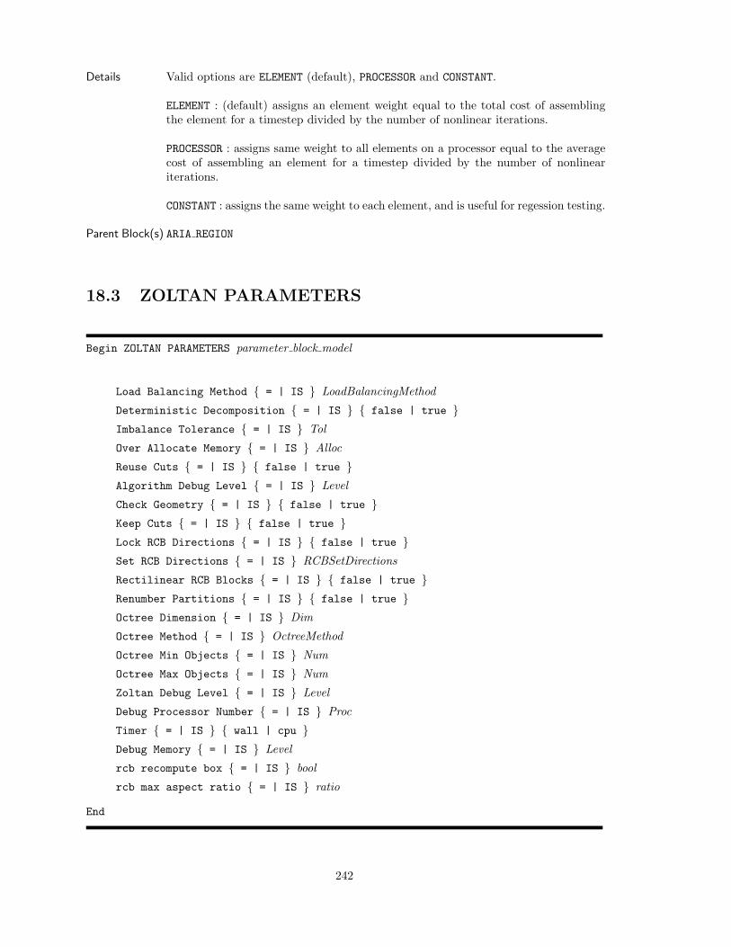
Details Valid options are ELEMENT (default), PROCESSOR and CONSTANT.
ELEMENT : (default) assigns an element weight equal to the total cost of assemblingthe element for a timestep divided by the number of nonlinear iterations.
PROCESSOR : assigns same weight to all elements on a processor equal to the averagecost of assembling an element for a timestep divided by the number of nonlineariterations.
CONSTANT : assigns the same weight to each element, and is useful for regession testing.
Parent Block(s) ARIA REGION
18.3 ZOLTAN PARAMETERS
Begin ZOLTAN PARAMETERS parameter block model
Load Balancing Method = | IS LoadBalancingMethod
Deterministic Decomposition = | IS false | true Imbalance Tolerance = | IS Tol
Over Allocate Memory = | IS Alloc
Reuse Cuts = | IS false | true Algorithm Debug Level = | IS Level
Check Geometry = | IS false | true Keep Cuts = | IS false | true Lock RCB Directions = | IS false | true Set RCB Directions = | IS RCBSetDirections
Rectilinear RCB Blocks = | IS false | true Renumber Partitions = | IS false | true Octree Dimension = | IS Dim
Octree Method = | IS OctreeMethod
Octree Min Objects = | IS Num
Octree Max Objects = | IS Num
Zoltan Debug Level = | IS Level
Debug Processor Number = | IS Proc
Timer = | IS wall | cpu Debug Memory = | IS Level
rcb recompute box = | IS bool
rcb max aspect ratio = | IS ratio
End
242
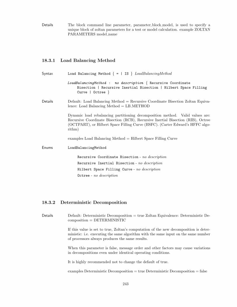
Details The block command line parameter, parameter block model, is used to specify aunique block of zoltan parameters for a test or model calculation. example ZOLTANPARAMETERS model name
18.3.1 Load Balancing Method
Syntax Load Balancing Method = | IS LoadBalancingMethod
LoadBalancingMethod : no description Recursive CoordinateBisection | Recursive Inertial Bisection | Hilbert Space FillingCurve | Octree
Details Default: Load Balancing Method = Recursive Coordinate Bisection Zoltan Equiva-lence: Load Balancing Method = LB METHOD
Dynamic load rebalancing partitioning decomposition method. Valid values are:Recursive Coordinate Bisection (RCB), Recursive Inertial Bisection (RIB), Octree(OCTPART), or Hilbert Space Filling Curve (HSFC). (Carter Edward’s HFFC algo-rithm)
examples Load Balancing Method = Hilbert Space Filling Curve
Enums LoadBalancingMethod
Recursive Coordinate Bisection - no description
Recursive Inertial Bisection - no description
Hilbert Space Filling Curve - no description
Octree - no description
18.3.2 Deterministic Decomposition
Details Default: Deterministic Decomposition = true Zoltan Equivalence: Deterministic De-composition = DETERMINISTIC
If this value is set to true, Zoltan’s computation of the new decomposition is deter-ministic: i.e. executing the same algorithm with the same input on the same numberof processors always produces the same results.
When this parameter is false, message order and other factors may cause variationsin decompositions even under identical operating conditions.
It is highly recommended not to change the default of true.
examples Deterministic Decomposition = true Deterministic Decomposition = false
243
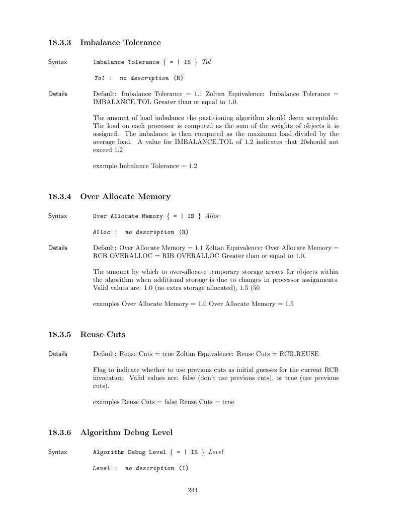
18.3.3 Imbalance Tolerance
Syntax Imbalance Tolerance = | IS Tol
Tol : no description (R)
Details Default: Imbalance Tolerance = 1.1 Zoltan Equivalence: Imbalance Tolerance =IMBALANCE TOL Greater than or equal to 1.0.
The amount of load imbalance the partitioning algorithm should deem acceptable.The load on each processor is computed as the sum of the weights of objects it isassigned. The imbalance is then computed as the maximum load divided by theaverage load. A value for IMBALANCE TOL of 1.2 indicates that 20should notexceed 1.2
example Imbalance Tolerance = 1.2
18.3.4 Over Allocate Memory
Syntax Over Allocate Memory = | IS Alloc
Alloc : no description (R)
Details Default: Over Allocate Memory = 1.1 Zoltan Equivalence: Over Allocate Memory =RCB OVERALLOC = RIB OVERALLOC Greater than or equal to 1.0.
The amount by which to over-allocate temporary storage arrays for objects withinthe algorithm when additional storage is due to changes in processor assignments.Valid values are: 1.0 (no extra storage allocated), 1.5 (50
examples Over Allocate Memory = 1.0 Over Allocate Memory = 1.5
18.3.5 Reuse Cuts
Details Default: Reuse Cuts = true Zoltan Equivalence: Reuse Cuts = RCB REUSE
Flag to indicate whether to use previous cuts as initial guesses for the current RCBinvocation. Valid values are: false (don’t use previous cuts), or true (use previouscuts).
examples Reuse Cuts = false Reuse Cuts = true
18.3.6 Algorithm Debug Level
Syntax Algorithm Debug Level = | IS Level
Level : no description (I)
244
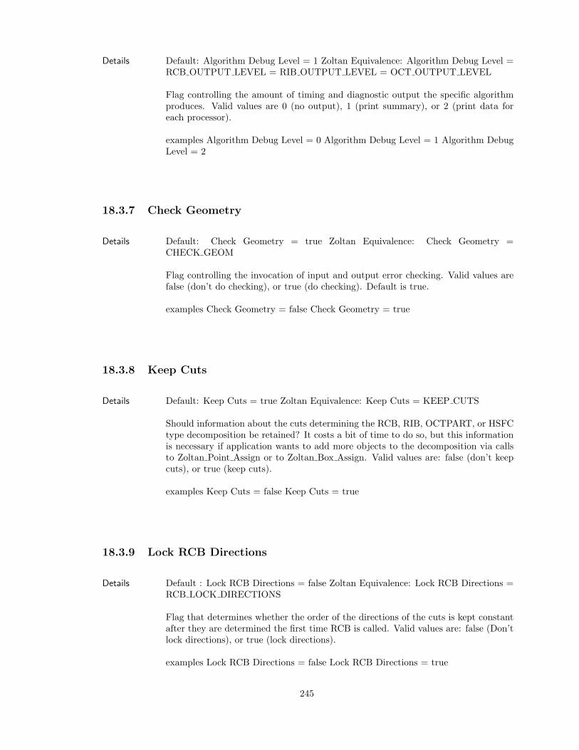
Details Default: Algorithm Debug Level = 1 Zoltan Equivalence: Algorithm Debug Level =RCB OUTPUT LEVEL = RIB OUTPUT LEVEL = OCT OUTPUT LEVEL
Flag controlling the amount of timing and diagnostic output the specific algorithmproduces. Valid values are 0 (no output), 1 (print summary), or 2 (print data foreach processor).
examples Algorithm Debug Level = 0 Algorithm Debug Level = 1 Algorithm DebugLevel = 2
18.3.7 Check Geometry
Details Default: Check Geometry = true Zoltan Equivalence: Check Geometry =CHECK GEOM
Flag controlling the invocation of input and output error checking. Valid values arefalse (don’t do checking), or true (do checking). Default is true.
examples Check Geometry = false Check Geometry = true
18.3.8 Keep Cuts
Details Default: Keep Cuts = true Zoltan Equivalence: Keep Cuts = KEEP CUTS
Should information about the cuts determining the RCB, RIB, OCTPART, or HSFCtype decomposition be retained? It costs a bit of time to do so, but this informationis necessary if application wants to add more objects to the decomposition via callsto Zoltan Point Assign or to Zoltan Box Assign. Valid values are: false (don’t keepcuts), or true (keep cuts).
examples Keep Cuts = false Keep Cuts = true
18.3.9 Lock RCB Directions
Details Default : Lock RCB Directions = false Zoltan Equivalence: Lock RCB Directions =RCB LOCK DIRECTIONS
Flag that determines whether the order of the directions of the cuts is kept constantafter they are determined the first time RCB is called. Valid values are: false (Don’tlock directions), or true (lock directions).
examples Lock RCB Directions = false Lock RCB Directions = true
245
18.3.10 Set RCB Directions
Syntax Set RCB Directions = | IS RCBSetDirections
RCBSetDirections : no description Do not order cuts | xyz | xzy |yzx | yxz | zxy | zyx
Details Default: Set RCB Directions = Do not order cuts Zoltan Equivalence: Set RCBDirections = RCB SET DIRECTIONS
Flag permits the order of cuts to be changed so that all of the cuts in any directionare done as a group. The number of cuts in each direction is determined and then thevalue of the parameter is used to determine the order that those cuts are made in.When 1D and 2D problems are partitioned, the directions corresponding to unuseddimensions are ignored. Valid values are: Do not order cuts, xyz, xzy, yzx, yxz, zxy,or zyx.
examples Set RCB Directions = Do not order cuts Set RCB Directions = xyz SetRCB Directions = xzy Set RCB Directions = yzx Set RCB Directions = yxz Set RCBDirections = zxy Set RCB Directions = zyx
Enums RCBSetDirections
Do not order cuts - no description
xyz - no description
xzy - no description
yzx - no description
yxz - no description
zxy - no description
zyx - no description
18.3.11 Rectilinear RCB Blocks
Details Default: Rectilinear RCB Blocks = false Zoltan Equivalence: Rectilinear RCB Blocks= RCB RECTILINEAR BLOCKS
Flag controlling the shape of the resulting regions. If this option is specified, thenwhen a cut is made, all of the dots located on the cut are moved to the same sideof the cut. The resulting regions are then rectilinear. When these dots are treatedas a group, then the resulting load balance may not be as good as when the groupof dots is split by the cut. Valid values are: false (move dots individually), or true(move dots in groups).
examples Rectilinear RCB Blocks = false Rectilinear RCB Blocks = true
246
18.3.12 Renumber Partitions
Details Default: Renumber Partitions = true Zoltan Equivalence: Renumber Partitions =REMAP
Flag to indicate whether to renumber partitions to mazimize overlap between the olddecomposition and the new decomposition (to reduce data movement from old to newdecompositions). Requests for remapping are ignored when, in the new decomposi-tion, a partition is spread across multiple processors or partition sizes are specifiedusing ”Set Partition Sizes”.
examples Renumber Partitions = false Renumber Partitions = true
18.3.13 Octree Dimension
Syntax Octree Dimension = | IS Dim
Dim : no description (I)
Details Default: Octree Dimension = 3 Zoltan Equivalence: Octree Dimension = OCT DIM
Specifies whether the 2D or 3D Octree algorithms should be used. The 3D algorithmscan be used for 2D problems, but much memory will be wasted to allow for a non-existent third dimension. Similarly, a 2D algorithm can be used for 3D surface meshesprovided that the surface can be projected to the xy-plane without overlapping points.Valid values are: 2 (use 2D algorithm), or 3 (use 3D algorithm).
examples Octree Dimension = 2 Octree Dimension = 3
18.3.14 Octree Method
Syntax Octree Method = | IS OctreeMethod
OctreeMethod : no description Morton Indexing | Grey Code |Hilbert
247
Details Default: Octree Method = Hilbert Zoltan Equivalence: OCT METHOD =oct method
The Space Filling Curve (SFC) to be used. To partition an octree, a traversal of thetree is used to define a global ordering on the leaves of the octree. This global orderingis often referred to as a Space-Filling Curve (SFC). The leaves of the octree can beeasily assigned to processors in a manner which equally distributes work by assigningslices of the ordered list to processors. Different tree-traversal algorithms producedifferent global orderings or SFCs, with some SFCs having better connectivity andpartition quality properties than others. Currently, Zoltan supports either MortonIndexing (i.e., Z-curve), Grey Code, or Hilbert SFCs. Morton Indexing and GreyCode SFCs are the simplest (and currently the fastest) of the SFC algorithms, butthey produce lower-quality partitions than the Hilbert SFC. Valid values are: MortonIndexing, Grey Code or Hilbert.
examples Octree Method = Morton Indexing Octree Method = Grey Code OctreeMethod = Hilbert
Enums OctreeMethod
Morton Indexing - no description
Grey Code - no description
Hilbert - no description
18.3.15 Octree Min Objects
Syntax Octree Min Objects = | IS Num
Num : no description (I)
Details Default: Octree Min Objects = 1 Zoltan Equivalence: Octree Min Objects =OCT MINOBJECTS
The minimum number of objects to allow in a leaf octant of the octree. Theseobjects will be assigned as a group to a processor, so this parameter helps define thegranularity of the load-balancing problem. Values
example Octree Min Objects = 5
18.3.16 Octree Max Objects
Syntax Octree Max Objects = | IS Num
Num : no description (I)
248
Details Default: Octree Max Objects = 1 Zoltan Equivalence: Octree Max Objects =OCT MAXOBJECTS
The maximum number of objects to allow in a leaf octant of the octree. Theseobjects will be assigned as a group to a processor, so this parameter helps define thegranularity of the load-balancing problem. Values greater than or equal to one areallowable.
example Octree Max Objects = 10
18.3.17 Zoltan Debug Level
Syntax Zoltan Debug Level = | IS Level
Level : no description (I)
Details Default: Zoltan Debug Level = 1 Zoltan Equivalence: Zoltan Debug Level = DE-BUG LEVEL 0 Quiet mode; no output unless an error or warning is produced. 1Values of all parameters set by Zoltan Set Param and used by the load-balancingmethod. 2 Timing information for Zoltan’s load-balancing and auto-migration rou-tines. 3 Timing information within load-balancing algorithms (support by algorithmsis optional). 4 5 Trace information (enter/exit) for major Zoltan interface routines(printed by the processor specified by the DEBUG PROCESSOR parameter). 6Trace information (enter/exit) for major Zoltan interface routines (printed by allprocessors). 7 More detailed trace information in major Zoltan interface routines. 8List of objects to be imported to and exported from each processor. 9 10 Maximumdebug output; may include algorithm-specific output. example Zoltan Debug Level= 5
18.3.18 Debug Processor Number
Syntax Debug Processor Number = | IS Proc
Proc : no description (I)
Details Default: Debug Processor = 0 Zoltan Equivalence: Debug Processor Number =DEBUG PROCESSOR
Processor number from which trace output should be printed when the zoltan pa-rameter, DEBUG LEVEL, is set to 5.
example Debug Processor Number = 2
249
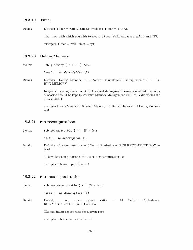
18.3.19 Timer
Details Default: Timer = wall Zoltan Equivalence: Timer = TIMER
The timer with which you wish to measure time. Valid values are WALL and CPU.
examples Timer = wall Timer = cpu
18.3.20 Debug Memory
Syntax Debug Memory = | IS Level
Level : no description (I)
Details Default: Debug Memory = 1 Zoltan Equivalence: Debug Memory = DE-BUG MEMORY
Integer indicating the amount of low-level debugging information about memory-allocation should be kept by Zoltan’s Memory Management utilities. Valid values are0, 1, 2, and 3
examples Debug Memory = 0 Debug Memory = 1 Debug Memory = 2 Debug Memory= 3
18.3.21 rcb recompute box
Syntax rcb recompute box = | IS bool
bool : no description (I)
Details Default: rcb recompute box = 0 Zoltan Equivalence: RCB RECOMPUTE BOX =bool
0, leave box computations off 1, turn box computations on
examples rcb recompute box = 1
18.3.22 rcb max aspect ratio
Syntax rcb max aspect ratio = | IS ratio
ratio : no description (I)
Details Default: rcb max aspect ratio = 10 Zoltan Equivalence:RCB MAX ASPECT RATIO = ratio
The maximum aspect ratio for a given part
examples rcb max aspect ratio = 5
250
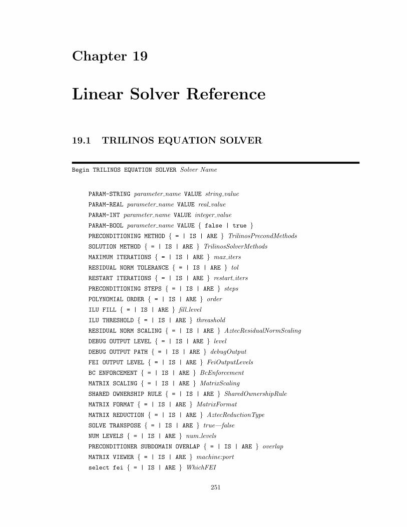
Chapter 19
Linear Solver Reference
19.1 TRILINOS EQUATION SOLVER
Begin TRILINOS EQUATION SOLVER Solver Name
PARAM-STRING parameter name VALUE string value
PARAM-REAL parameter name VALUE real value
PARAM-INT parameter name VALUE integer value
PARAM-BOOL parameter name VALUE false | true PRECONDITIONING METHOD = | IS | ARE TrilinosPrecondMethods
SOLUTION METHOD = | IS | ARE TrilinosSolverMethods
MAXIMUM ITERATIONS = | IS | ARE max iters
RESIDUAL NORM TOLERANCE = | IS | ARE tol
RESTART ITERATIONS = | IS | ARE restart iters
PRECONDITIONING STEPS = | IS | ARE steps
POLYNOMIAL ORDER = | IS | ARE order
ILU FILL = | IS | ARE fill level
ILU THRESHOLD = | IS | ARE threashold
RESIDUAL NORM SCALING = | IS | ARE AztecResidualNormScaling
DEBUG OUTPUT LEVEL = | IS | ARE level
DEBUG OUTPUT PATH = | IS | ARE debugOutput
FEI OUTPUT LEVEL = | IS | ARE FeiOutputLevels
BC ENFORCEMENT = | IS | ARE BcEnforcement
MATRIX SCALING = | IS | ARE MatrixScaling
SHARED OWNERSHIP RULE = | IS | ARE SharedOwnershipRule
MATRIX FORMAT = | IS | ARE MatrixFormat
MATRIX REDUCTION = | IS | ARE AztecReductionType
SOLVE TRANSPOSE = | IS | ARE true—false
NUM LEVELS = | IS | ARE num levels
PRECONDITIONER SUBDOMAIN OVERLAP = | IS | ARE overlap
MATRIX VIEWER = | IS | ARE machine:port
select fei = | IS | ARE WhichFEI
251
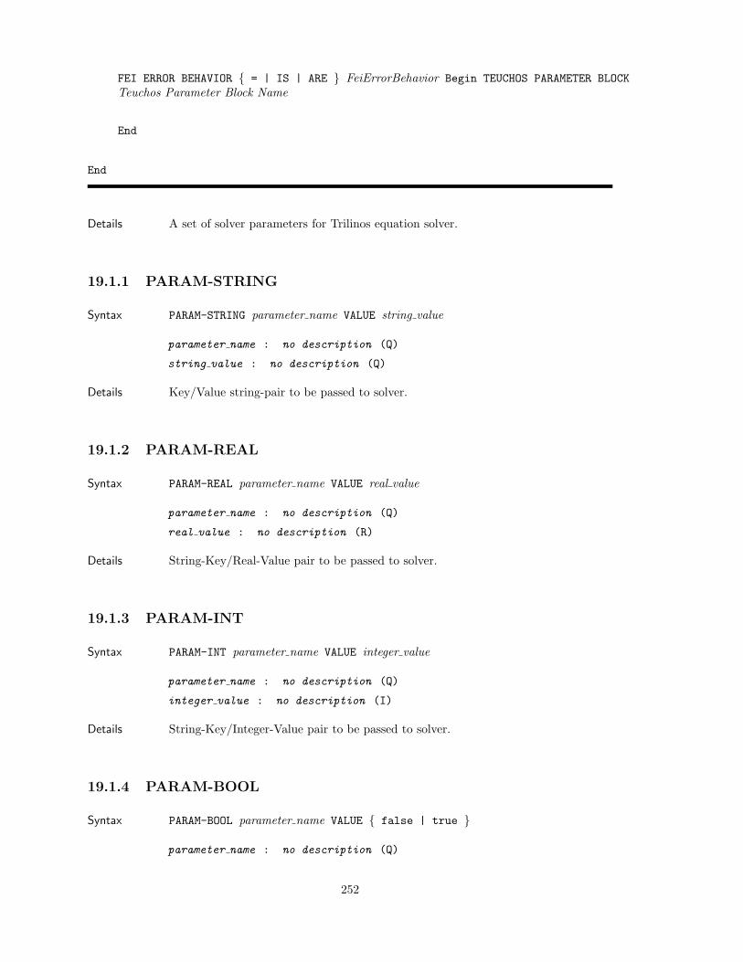
FEI ERROR BEHAVIOR = | IS | ARE FeiErrorBehavior Begin TEUCHOS PARAMETER BLOCKTeuchos Parameter Block Name
End
End
Details A set of solver parameters for Trilinos equation solver.
19.1.1 PARAM-STRING
Syntax PARAM-STRING parameter name VALUE string value
parameter name : no description (Q)
string value : no description (Q)
Details Key/Value string-pair to be passed to solver.
19.1.2 PARAM-REAL
Syntax PARAM-REAL parameter name VALUE real value
parameter name : no description (Q)
real value : no description (R)
Details String-Key/Real-Value pair to be passed to solver.
19.1.3 PARAM-INT
Syntax PARAM-INT parameter name VALUE integer value
parameter name : no description (Q)
integer value : no description (I)
Details String-Key/Integer-Value pair to be passed to solver.
19.1.4 PARAM-BOOL
Syntax PARAM-BOOL parameter name VALUE false | true
parameter name : no description (Q)
252
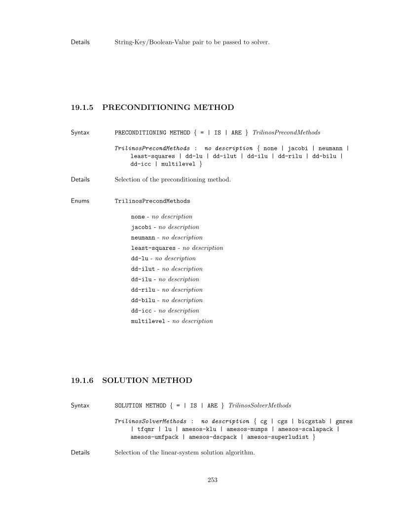
Details String-Key/Boolean-Value pair to be passed to solver.
19.1.5 PRECONDITIONING METHOD
Syntax PRECONDITIONING METHOD = | IS | ARE TrilinosPrecondMethods
TrilinosPrecondMethods : no description none | jacobi | neumann |least-squares | dd-lu | dd-ilut | dd-ilu | dd-rilu | dd-bilu |dd-icc | multilevel
Details Selection of the preconditioning method.
Enums TrilinosPrecondMethods
none - no description
jacobi - no description
neumann - no description
least-squares - no description
dd-lu - no description
dd-ilut - no description
dd-ilu - no description
dd-rilu - no description
dd-bilu - no description
dd-icc - no description
multilevel - no description
19.1.6 SOLUTION METHOD
Syntax SOLUTION METHOD = | IS | ARE TrilinosSolverMethods
TrilinosSolverMethods : no description cg | cgs | bicgstab | gmres| tfqmr | lu | amesos-klu | amesos-mumps | amesos-scalapack |amesos-umfpack | amesos-dscpack | amesos-superludist
Details Selection of the linear-system solution algorithm.
253
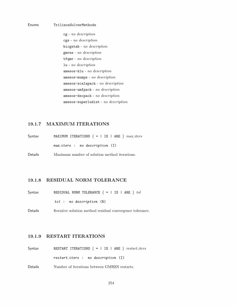
Enums TrilinosSolverMethods
cg - no description
cgs - no description
bicgstab - no description
gmres - no description
tfqmr - no description
lu - no description
amesos-klu - no description
amesos-mumps - no description
amesos-scalapack - no description
amesos-umfpack - no description
amesos-dscpack - no description
amesos-superludist - no description
19.1.7 MAXIMUM ITERATIONS
Syntax MAXIMUM ITERATIONS = | IS | ARE max iters
max iters : no description (I)
Details Maximum number of solution method iterations.
19.1.8 RESIDUAL NORM TOLERANCE
Syntax RESIDUAL NORM TOLERANCE = | IS | ARE tol
tol : no description (R)
Details Iterative solution method residual convergence tolerance.
19.1.9 RESTART ITERATIONS
Syntax RESTART ITERATIONS = | IS | ARE restart iters
restart iters : no description (I)
Details Number of iterations between GMRES restarts.
254
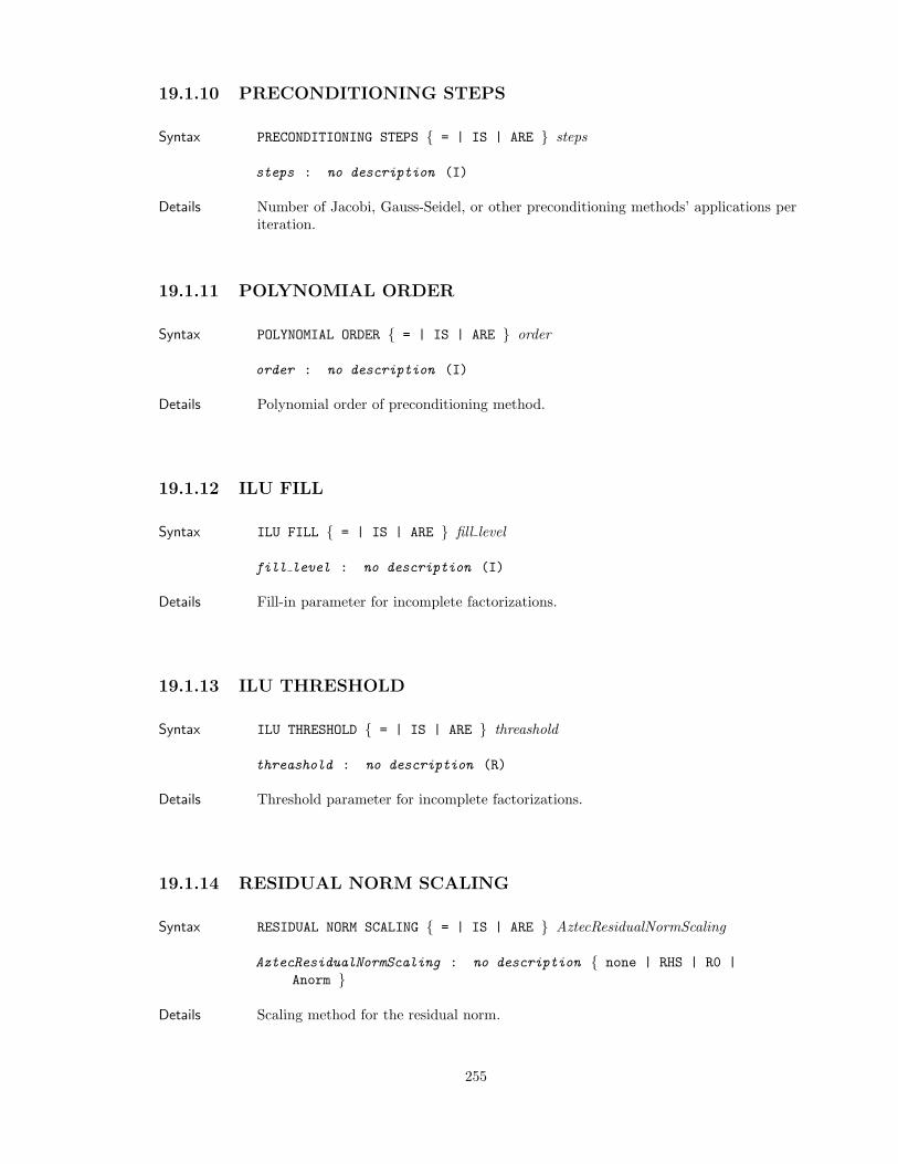
19.1.10 PRECONDITIONING STEPS
Syntax PRECONDITIONING STEPS = | IS | ARE steps
steps : no description (I)
Details Number of Jacobi, Gauss-Seidel, or other preconditioning methods’ applications periteration.
19.1.11 POLYNOMIAL ORDER
Syntax POLYNOMIAL ORDER = | IS | ARE order
order : no description (I)
Details Polynomial order of preconditioning method.
19.1.12 ILU FILL
Syntax ILU FILL = | IS | ARE fill level
fill level : no description (I)
Details Fill-in parameter for incomplete factorizations.
19.1.13 ILU THRESHOLD
Syntax ILU THRESHOLD = | IS | ARE threashold
threashold : no description (R)
Details Threshold parameter for incomplete factorizations.
19.1.14 RESIDUAL NORM SCALING
Syntax RESIDUAL NORM SCALING = | IS | ARE AztecResidualNormScaling
AztecResidualNormScaling : no description none | RHS | R0 |Anorm
Details Scaling method for the residual norm.
255
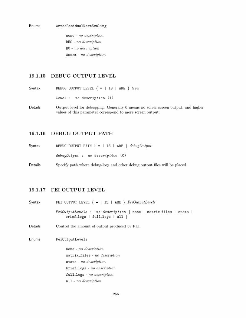
Enums AztecResidualNormScaling
none - no description
RHS - no description
R0 - no description
Anorm - no description
19.1.15 DEBUG OUTPUT LEVEL
Syntax DEBUG OUTPUT LEVEL = | IS | ARE level
level : no description (I)
Details Output level for debugging. Generally 0 means no solver screen output, and highervalues of this parameter correspond to more screen output.
19.1.16 DEBUG OUTPUT PATH
Syntax DEBUG OUTPUT PATH = | IS | ARE debugOutput
debugOutput : no description (C)
Details Specify path where debug-logs and other debug output files will be placed.
19.1.17 FEI OUTPUT LEVEL
Syntax FEI OUTPUT LEVEL = | IS | ARE FeiOutputLevels
FeiOutputLevels : no description none | matrix files | stats |brief logs | full logs | all
Details Control the amount of output produced by FEI.
Enums FeiOutputLevels
none - no description
matrix files - no description
stats - no description
brief logs - no description
full logs - no description
all - no description
256
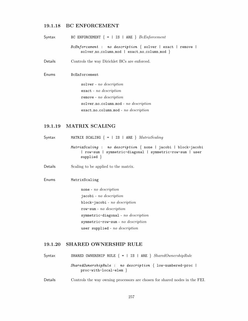
19.1.18 BC ENFORCEMENT
Syntax BC ENFORCEMENT = | IS | ARE BcEnforcement
BcEnforcement : no description solver | exact | remove |solver no column mod | exact no column mod
Details Controls the way Dirichlet BCs are enforced.
Enums BcEnforcement
solver - no description
exact - no description
remove - no description
solver no column mod - no description
exact no column mod - no description
19.1.19 MATRIX SCALING
Syntax MATRIX SCALING = | IS | ARE MatrixScaling
MatrixScaling : no description none | jacobi | block-jacobi| row-sum | symmetric-diagonal | symmetric-row-sum | usersupplied
Details Scaling to be applied to the matrix.
Enums MatrixScaling
none - no description
jacobi - no description
block-jacobi - no description
row-sum - no description
symmetric-diagonal - no description
symmetric-row-sum - no description
user supplied - no description
19.1.20 SHARED OWNERSHIP RULE
Syntax SHARED OWNERSHIP RULE = | IS | ARE SharedOwnershipRule
SharedOwnershipRule : no description low-numbered-proc |proc-with-local-elem
Details Controls the way owning processors are chosen for shared nodes in the FEI.
257
Enums SharedOwnershipRule
low-numbered-proc - no description
proc-with-local-elem - no description
19.1.21 MATRIX FORMAT
Syntax MATRIX FORMAT = | IS | ARE MatrixFormat
MatrixFormat : no description MSR | VBR | CSR
Details Storage format for the matrix.
Enums MatrixFormat
MSR - no description
VBR - no description
CSR - no description
19.1.22 MATRIX REDUCTION
Syntax MATRIX REDUCTION = | IS | ARE AztecReductionType
AztecReductionType : no description fei-remove-slaves
Details Remove constraint equations from matrix.
Enums AztecReductionType
fei-remove-slaves - no description
19.1.23 SOLVE TRANSPOSE
Syntax SOLVE TRANSPOSE = | IS | ARE true—false
true|false : no description (C)
Details Whether to solve for transpose of system matrix.
19.1.24 NUM LEVELS
Syntax NUM LEVELS = | IS | ARE num levels
num levels : no description (I)
258
Details Number of levels for multi-level/multi-grid solvers.
19.1.25 PRECONDITIONER SUBDOMAIN OVERLAP
Syntax PRECONDITIONER SUBDOMAIN OVERLAP = | IS | ARE overlap
overlap : no description (I)
Details Ovrlap of Schwarz subdomains (eg, 0,1 or 2).
19.1.26 MATRIX VIEWER
Syntax MATRIX VIEWER = | IS | ARE machine:port
machine:port : no description (C)
Details Host and port-number where matvis is running.
19.1.27 select fei
Syntax select fei = | IS | ARE WhichFEI
WhichFEI : no description old | new
Details Selection of old vs new fei.
Enums WhichFEI
old - no description
new - no description
19.1.28 FEI ERROR BEHAVIOR
Syntax FEI ERROR BEHAVIOR = | IS | ARE FeiErrorBehavior
FeiErrorBehavior : no description returncode | abort
Details Set FEI error behavior to abort (rather than the default which is to simply print amessage and return an integer error code).
Enums FeiErrorBehavior
returncode - no description
abort - no description
259
19.2 TEUCHOS PARAMETER BLOCK
Begin TEUCHOS PARAMETER BLOCK Teuchos Parameter Block Name
PARAM-STRING parameter name VALUE string value
PARAM-REAL parameter name VALUE real value
PARAM-INT parameter name VALUE integer value
PARAM-BOOL parameter name VALUE false | true PARAM-SUBLIST parameter name VALUE block name
End
Details A block to set a Teuchos parameter list.
19.2.1 PARAM-STRING
Syntax PARAM-STRING parameter name VALUE string value
parameter name : no description (Q)
string value : no description (Q)
Details Key/Value string-pair to be passed to solver.
19.2.2 PARAM-REAL
Syntax PARAM-REAL parameter name VALUE real value
parameter name : no description (Q)
real value : no description (R)
Details String-Key/Real-Value pair to be passed to solver.
19.2.3 PARAM-INT
Syntax PARAM-INT parameter name VALUE integer value
parameter name : no description (Q)
integer value : no description (I)
Details String-Key/Integer-Value pair to be passed to solver.
260
19.2.4 PARAM-BOOL
Syntax PARAM-BOOL parameter name VALUE false | true
parameter name : no description (Q)
Details String-Key/Boolean-Value pair to be passed to solver.
19.2.5 PARAM-SUBLIST
Syntax PARAM-SUBLIST parameter name VALUE block name
parameter name : no description (Q)
block name : no description (C)
Details String-Key/String-Value pair to designate another Teuchos block as a sublist to thisblock.
19.3 AZTEC EQUATION SOLVER
Begin AZTEC EQUATION SOLVER Solver Name
PARAM-STRING parameter name VALUE string value
PARAM-REAL parameter name VALUE real value
PARAM-INT parameter name VALUE integer value
SOLUTION METHOD = | IS | ARE AztecSolverMethods
PRECONDITIONING METHOD = | IS | ARE AztecPrecondMethods
MAXIMUM ITERATIONS = | IS | ARE max iters
RESIDUAL NORM TOLERANCE = | IS | ARE tol
RESTART ITERATIONS = | IS | ARE restart iters
PRECONDITIONING STEPS = | IS | ARE steps
POLYNOMIAL ORDER = | IS | ARE order
ILU FILL = | IS | ARE fill level
ILU THRESHOLD = | IS | ARE threashold
RESIDUAL NORM SCALING = | IS | ARE AztecResidualNormScaling
ILU OMEGA = | IS | ARE value
DEBUG OUTPUT LEVEL = | IS | ARE level
DEBUG OUTPUT PATH = | IS | ARE debugOutput
FEI OUTPUT LEVEL = | IS | ARE FeiOutputLevels
ORTHOG METHOD = | IS | ARE OrthogMethod
BC ENFORCEMENT = | IS | ARE BcEnforcement
261
MATRIX SCALING = | IS | ARE MatrixScaling
SHARED OWNERSHIP RULE = | IS | ARE SharedOwnershipRule
MATRIX FORMAT = | IS | ARE MatrixFormat
MATRIX REDUCTION = | IS | ARE AztecReductionType
NUM LEVELS = | IS | ARE num levels
PRECONDITIONER SUBDOMAIN OVERLAP = | IS | ARE overlap
MATRIX VIEWER = | IS | ARE machine:port
select fei = | IS | ARE WhichFEI
FEI ERROR BEHAVIOR = | IS | ARE FeiErrorBehavior
End
Details A set of solver parameters for Aztec equation solver.
19.3.1 PARAM-STRING
Syntax PARAM-STRING parameter name VALUE string value
parameter name : no description (Q)
string value : no description (Q)
Details Key/Value string-pair to be passed to solver.
19.3.2 PARAM-REAL
Syntax PARAM-REAL parameter name VALUE real value
parameter name : no description (Q)
real value : no description (R)
Details String-Key/Real-Value pair to be passed to solver.
19.3.3 PARAM-INT
Syntax PARAM-INT parameter name VALUE integer value
parameter name : no description (Q)
integer value : no description (I)
Details String-Key/Integer-Value pair to be passed to solver.
262
19.3.4 SOLUTION METHOD
Syntax SOLUTION METHOD = | IS | ARE AztecSolverMethods
AztecSolverMethods : no description cg | cgs | bicgstab | gmres |tfqmr | lu
Details Selection of the linear-system solution algorithm.
Enums AztecSolverMethods
cg - no description
cgs - no description
bicgstab - no description
gmres - no description
tfqmr - no description
lu - no description
19.3.5 PRECONDITIONING METHOD
Syntax PRECONDITIONING METHOD = | IS | ARE AztecPrecondMethods
AztecPrecondMethods : no description none | jacobi | neumann |least-squares | symmetric-gauss-seidel | dd-lu | dd-ilut | dd-ilu| dd-rilu | dd-bilu | dd-icc
Details Selection of the equation preconditioning method.
Enums AztecPrecondMethods
none - no description
jacobi - no description
neumann - no description
least-squares - no description
symmetric-gauss-seidel - no description
dd-lu - no description
dd-ilut - no description
dd-ilu - no description
dd-rilu - no description
dd-bilu - no description
dd-icc - no description
263
19.3.6 MAXIMUM ITERATIONS
Syntax MAXIMUM ITERATIONS = | IS | ARE max iters
max iters : no description (I)
Details Maximum number of solution method iterations.
19.3.7 RESIDUAL NORM TOLERANCE
Syntax RESIDUAL NORM TOLERANCE = | IS | ARE tol
tol : no description (R)
Details Iterative solution method residual convergence tolerance.
19.3.8 RESTART ITERATIONS
Syntax RESTART ITERATIONS = | IS | ARE restart iters
restart iters : no description (I)
Details Number of iterations between GMRES restarts.
19.3.9 PRECONDITIONING STEPS
Syntax PRECONDITIONING STEPS = | IS | ARE steps
steps : no description (I)
Details Number of Jacobi, Gauss-Seidel, or other preconditioning methods’ applications periteration.
19.3.10 POLYNOMIAL ORDER
Syntax POLYNOMIAL ORDER = | IS | ARE order
order : no description (I)
Details Polynomial order of preconditioning method.
264
19.3.11 ILU FILL
Syntax ILU FILL = | IS | ARE fill level
fill level : no description (I)
Details Fill-in parameter for incomplete factorizations.
19.3.12 ILU THRESHOLD
Syntax ILU THRESHOLD = | IS | ARE threashold
threashold : no description (R)
Details Threshold parameter for incomplete factorizations.
19.3.13 RESIDUAL NORM SCALING
Syntax RESIDUAL NORM SCALING = | IS | ARE AztecResidualNormScaling
AztecResidualNormScaling : no description none | RHS | R0 |Anorm
Details Scaling method for the residual norm.
Enums AztecResidualNormScaling
none - no description
RHS - no description
R0 - no description
Anorm - no description
19.3.14 ILU OMEGA
Syntax ILU OMEGA = | IS | ARE value
value : no description (R)
Details Omega parameter, dd-rilu uses ILU(k,w), w==omega
265
19.3.15 DEBUG OUTPUT LEVEL
Syntax DEBUG OUTPUT LEVEL = | IS | ARE level
level : no description (I)
Details Output level for debugging. Generally 0 means no solver screen output, and highervalues of this parameter correspond to more screen output.
19.3.16 DEBUG OUTPUT PATH
Syntax DEBUG OUTPUT PATH = | IS | ARE debugOutput
debugOutput : no description (C)
Details Specify path where debug-logs and other debug output files will be placed.
19.3.17 FEI OUTPUT LEVEL
Syntax FEI OUTPUT LEVEL = | IS | ARE FeiOutputLevels
FeiOutputLevels : no description none | matrix files | stats |brief logs | full logs | all
Details Control the amount of output produced by FEI.
Enums FeiOutputLevels
none - no description
matrix files - no description
stats - no description
brief logs - no description
full logs - no description
all - no description
19.3.18 ORTHOG METHOD
Syntax ORTHOG METHOD = | IS | ARE OrthogMethod
OrthogMethod : no description modified | classical
Details User can choose orthogonalization method used by Aztec GMRES.
266
Enums OrthogMethod
modified - no description
classical - no description
19.3.19 BC ENFORCEMENT
Syntax BC ENFORCEMENT = | IS | ARE BcEnforcement
BcEnforcement : no description solver | exact | remove |solver no column mod | exact no column mod
Details Controls the way Dirichlet BCs are enforced.
Enums BcEnforcement
solver - no description
exact - no description
remove - no description
solver no column mod - no description
exact no column mod - no description
19.3.20 MATRIX SCALING
Syntax MATRIX SCALING = | IS | ARE MatrixScaling
MatrixScaling : no description none | jacobi | block-jacobi| row-sum | symmetric-diagonal | symmetric-row-sum | usersupplied
Details Scaling to be applied to the matrix.
Enums MatrixScaling
none - no description
jacobi - no description
block-jacobi - no description
row-sum - no description
symmetric-diagonal - no description
symmetric-row-sum - no description
user supplied - no description
267
19.3.21 SHARED OWNERSHIP RULE
Syntax SHARED OWNERSHIP RULE = | IS | ARE SharedOwnershipRule
SharedOwnershipRule : no description low-numbered-proc |proc-with-local-elem
Details Controls the way owning processors are chosen for shared nodes in the FEI.
Enums SharedOwnershipRule
low-numbered-proc - no description
proc-with-local-elem - no description
19.3.22 MATRIX FORMAT
Syntax MATRIX FORMAT = | IS | ARE MatrixFormat
MatrixFormat : no description MSR | VBR | CSR
Details Storage format for the matrix.
Enums MatrixFormat
MSR - no description
VBR - no description
CSR - no description
19.3.23 MATRIX REDUCTION
Syntax MATRIX REDUCTION = | IS | ARE AztecReductionType
AztecReductionType : no description fei-remove-slaves
Details Remove constraint equations from matrix.
Enums AztecReductionType
fei-remove-slaves - no description
19.3.24 NUM LEVELS
Syntax NUM LEVELS = | IS | ARE num levels
num levels : no description (I)
268
Details Number of levels for multi-level/multi-grid solvers.
19.3.25 PRECONDITIONER SUBDOMAIN OVERLAP
Syntax PRECONDITIONER SUBDOMAIN OVERLAP = | IS | ARE overlap
overlap : no description (I)
Details Ovrlap of Schwarz subdomains (eg, 0,1 or 2).
19.3.26 MATRIX VIEWER
Syntax MATRIX VIEWER = | IS | ARE machine:port
machine:port : no description (C)
Details Host and port-number where matvis is running.
19.3.27 select fei
Syntax select fei = | IS | ARE WhichFEI
WhichFEI : no description old | new
Details Selection of old vs new fei.
Enums WhichFEI
old - no description
new - no description
19.3.28 FEI ERROR BEHAVIOR
Syntax FEI ERROR BEHAVIOR = | IS | ARE FeiErrorBehavior
FeiErrorBehavior : no description returncode | abort
Details Set FEI error behavior to abort (rather than the default which is to simply print amessage and return an integer error code).
Enums FeiErrorBehavior
returncode - no description
abort - no description
269

270
Chapter 20
Postprocessing Operations
20.1 POSTPROCESS
The POSTPROCESS line command is used to add extra calculations to a region, that are carriedout after the region’s main calculations. They also add extra fields to the Exodus II output file.
Syntax POSTPROCESS OPERATION [[] SUBINDEX] ON MESH PART [param1 spec1]
Description Performs the postprocessing operation OPERATION on the mesh entity associated withMESH PART .
Details The MESH PART may be sideset (e.g., “surface 10”) or element block (e.g.,“block 1”).
Parent Block(s) ARIA REGION
Operation
FLUID TRACTION
Description Computes the value of n · σ on a surface where n is the unit normal tothe surface and σ is the fluid stress tensor.
Details The fluid tractions are computed on the surface element nodes ofMESH PART . The surface element corresponds to a face of the parentelement for the fluid MOMENTUM equation.
271
Operation
FLUID FORCE
Parameters [USING INTERP ]
Description Computes the equivalent nodal point fluid force based upon the integralof n · σ on a surface where n is the unit normal to the surface and σ isthe fluid stress tensor.
Details By default the equivalent nodal forces are computed on the parent ele-ment for the fluid MOMENTUM equation. The USING INTERP option isprovided to allow projection of the equivalent nodal force onto elementnodes corresponding to the INTERP surface element. A valid INTERP
entry can only be the parent element or a sub-element of the parentelement. Admissible values of INTERP are Q1, Q2, QS2, T1 and T2.
Operation
ELECTRIC FIELD
Parameters [USING INTERP ]
Description Computes the electric field.
Details Computes the electric field as
E = −∇V
Currently, this only works on the default voltage (subindex=-1)
Operation
CURRENT
Parameters [USING INTERP ]
Example Postprocess Current on block 1
Description Computes the electrical current.
Details Computes the current asJ = −σe∇V
where V is the voltage (electric potential) and σe is the electrical con-ductivity.
272
Operation
PRESSURE
Parameters [USING INTERP ]
Description Computes the pressure at all of the nodes. This is useful if the pressuredegree of freedom uses a lower order finite element interpolation than themesh, e.g., linear (Q1) pressure on a quadratic (Q2) mesh, or constant-over-the-element (P0) vs. linear (Q1).
Details Currently, the value assigned to a node is the average value based on thenumber of elements that share that node. There’s no slick projection orweighting involved. Therefore, convergence studies based on the pressurewill seriously underestimate the fidelity of a calculation, until this isfixed.
Operation
TEMPERATURE
Parameters [USING INTERP ]
Description Computes the temperature on all of the nodes. This is useful if thetemperature degree of freedom uses a lower order interpolation that themesh, e.g., linear (Q1) temperature on a quadratic (Q2) mesh.
Details Currently, the value assigned to a node is the average value based on thenumber of elements that share that node. There’s no slick projection orweighting scheme involved.
Operation
DENSITY
Parameters [USING INTERP ]
Description Computes the density material property so that it’s available for out-put.
Details The value assigned to a node is the average value based on the number ofelements that share that node. There’s no slick projection or weightinginvolved.
273
Operation
VISCOSITY
Parameters [USING INTERP ]
Description Computes the viscosity material property so that it’s available for out-put.
Details No details to speak of. Oh, well there’s one detail you may care about:The value assigned to a node is the average value based on the number ofelements that share that node. There’s no slick projection or weightinginvolved.
Operation
THERMAL CONDUCTIVITY
Parameters [USING INTERP ]
Description Computes the thermal conductivity material property so that it’s avail-able for output.
Details No details to speak of. Oh, well there’s one detail you may care about:The value assigned to a node is the average value based on the number ofelements that share that node. There’s no slick projection or weightinginvolved.
Operation
SPECIFIC HEAT
Parameters [USING INTERP ]
Description Computes the specific heat material property so that it’s available foroutput.
Details No details to speak of. Oh, well there’s one detail you may care about:The value assigned to a node is the average value based on the number ofelements that share that node. There’s no slick projection or weightinginvolved.
274
Operation
PROJECTED FLUID STRESS XX
Parameters [USING INTERP ]
Description Computes one of the stress tensor components, calculated from the stressprojection equation, at all of the nodes. This is useful if this degree offreedom uses a lower order finite element interpolation than the mesh,e.g., linear (Q1) pressure on a quadratic (Q2) mesh, or constant-over-the-element (P0) vs. linear (Q1).
Details XX, here, may be equal to XX, XY, YX, and YY for 2D, and XX,XY, XZ, YX, YY, YZ, ZX, ZY, and ZZ for 3D. In other words eachcomponent of the tensor must be individually postprocessed and outputto an exodus file.
275

276
Chapter 21
Enclosure Radiation Reference
21.1 VIEWFACTOR CALCULATION
Begin VIEWFACTOR CALCULATION vf calc
BSP TREE MAX DEPTH = | IS DEPTH AND MIN LIST LENGTH = | IS L
GEOMETRIC TOLERANCE = | IS n
COMPUTE RULE = | IS VFComputeRule
HEMICUBE RESOLUTION = | IS n
HEMICUBE MAX SUBDIVIDES = | IS n
HEMICUBE MIN SEPARATION = | IS n
PAIRWISE NUMBER OF VISIBILITY SAMPLES = | IS n
PAIRWISE VISIBILITY SAMPLE RULE = | IS AVSampleRule
PAIRWISE NUMBER OF MONTE CARLO SAMPLES = | IS n
PAIRWISE MONTE CARLO SAMPLE RULE = | IS AMCSampleRule
PAIRWISE MONTE CARLO TOL1 = | IS real value
PAIRWISE MONTE CARLO TOL2 = | IS real value
OUTPUT RULE = | IS OutputRule
NUMBER OF ROTATIONS = | IS n
X-Y PLANE SYMMETRY
X-Z PLANE SYMMETRY
Y-Z PLANE SYMMETRY
End
Details This block command specifies a radiation enclosure and is used to define a methodfor calculating view factors. The parameter for this block corresponds to an instanceof a radiation enclosure mechanics.
277
21.1.1 BSP TREE MAX DEPTH
Syntax BSP TREE MAX DEPTH = | IS DEPTH AND MIN LIST LENGTH = | IS L
DEPTH : no description (I)
L : no description (I)
Details This line command sets the BSP tree parameters.
21.1.2 GEOMETRIC TOLERANCE
Syntax GEOMETRIC TOLERANCE = | IS n
n : no description (R)
Details Set the geometric tolerance
21.1.3 COMPUTE RULE
Syntax COMPUTE RULE = | IS VFComputeRule
VFComputeRule : no description PAIRWISE | HEMICUBE | READ
Details This line command sets the method for computing the view factors for this enclosure.Default value is HEMICUBE
Enums VFComputeRule
PAIRWISE - no description
HEMICUBE - no description
READ - no description
21.1.4 HEMICUBE RESOLUTION
Syntax HEMICUBE RESOLUTION = | IS n
n : no description (I)
Details Set the hemicube resolution
278
21.1.5 HEMICUBE MAX SUBDIVIDES
Syntax HEMICUBE MAX SUBDIVIDES = | IS n
n : no description (I)
Details Set the upper limit of hemicube subdivides
21.1.6 HEMICUBE MIN SEPARATION
Syntax HEMICUBE MIN SEPARATION = | IS n
n : no description (R)
Details Set the hemicube minimum seperation
21.1.7 PAIRWISE NUMBER OF VISIBILITY SAMPLES
Syntax PAIRWISE NUMBER OF VISIBILITY SAMPLES = | IS n
n : no description (I)
Details Set the pairwise number visibility sample points
21.1.8 PAIRWISE VISIBILITY SAMPLE RULE
Syntax PAIRWISE VISIBILITY SAMPLE RULE = | IS AVSampleRule
AVSampleRule : no description RANDOM | UNIFORM | JITTER |HALTON
Details Set the pairwise visibility sample rule
Enums AVSampleRule
RANDOM - no description
UNIFORM - no description
JITTER - no description
HALTON - no description
279
21.1.9 PAIRWISE NUMBER OF MONTE CARLO SAMPLES
Syntax PAIRWISE NUMBER OF MONTE CARLO SAMPLES = | IS n
n : no description (I)
Details Set the pairwise number of Monte Carlo sample points
21.1.10 PAIRWISE MONTE CARLO SAMPLE RULE
Syntax PAIRWISE MONTE CARLO SAMPLE RULE = | IS AMCSampleRule
AMCSampleRule : no description RANDOM | UNIFORM | JITTER |HALTON
Details
Enums AMCSampleRule
RANDOM - no description
UNIFORM - no description
JITTER - no description
HALTON - no description
21.1.11 PAIRWISE MONTE CARLO TOL1
Syntax PAIRWISE MONTE CARLO TOL1 = | IS real value
real value : no description (R)
Details Set first of two convergence checks for Monte Carlo integration
21.1.12 PAIRWISE MONTE CARLO TOL2
Syntax PAIRWISE MONTE CARLO TOL2 = | IS real value
real value : no description (R)
Details Set second of two convergence checks for Monte Carlo integration
280
21.1.13 OUTPUT RULE
Syntax OUTPUT RULE = | IS OutputRule
OutputRule : no description NONE | SUMMARY | VERBOSE
Details Toggle verbose reporting
Enums OutputRule
NONE - no description
SUMMARY - no description
VERBOSE - no description
21.1.14 NUMBER OF ROTATIONS
Syntax NUMBER OF ROTATIONS = | IS n
n : no description (I)
Details Set the number of internal rotations for 2D axisymmetric geometry or 3D geometrywith rotation symmetry. The default value is 1
21.1.15 X-Y PLANE SYMMETRY
Details Specifies symmetry about the X-Y plane.
21.1.16 X-Z PLANE SYMMETRY
Details Specifies symmetry about the X-Z plane.
21.1.17 Y-Z PLANE SYMMETRY
Details Specifies symmetry about the Y-Z plane.
21.2 RADIOSITY SOLVER
Begin RADIOSITY SOLVER Boundary condition instance name
COUPLING = | IS RadCouplingRule
281
SOLVER = | IS RadSolveRule
CONVERGENCE TOLERANCE = | IS tolerance
MAXIMUM ITERATIONS = | IS M
OUTPUT RULE = | IS OutputRule
End
Details Specifies a radiation enclosure. Corresponds to an instance of radiation enclosuremechanics.
21.2.1 COUPLING
Syntax COUPLING = | IS RadCouplingRule
RadCouplingRule : no description MASON | LAGGED
Details Specifies linearization method. Default is MASON.
Enums RadCouplingRule
MASON - no description
LAGGED - no description
21.2.2 SOLVER
Syntax SOLVER = | IS RadSolveRule
RadSolveRule : no description CHAPARRAL GMRES | CHAPARRAL CG |COUPLED
Details Chaparal solver selection for radiosity system. Default is CHAPARRAL CG.
Enums RadSolveRule
CHAPARRAL GMRES - no description
CHAPARRAL CG - no description
COUPLED - no description
21.2.3 CONVERGENCE TOLERANCE
Syntax CONVERGENCE TOLERANCE = | IS tolerance
tolerance : no description (R)
282
Details Sets convergence tolerance. Default value is 1.0e-6.
21.2.4 MAXIMUM ITERATIONS
Syntax MAXIMUM ITERATIONS = | IS M
M : no description (I)
Details Sets maximum number of iterations. Default value is 300.
21.2.5 OUTPUT RULE
Syntax OUTPUT RULE = | IS OutputRule
OutputRule : no description NONE | SUMMARY | VERBOSE
Details Sets the information reporting level. Default is NONE.
Enums OutputRule
NONE - no description
SUMMARY - no description
VERBOSE - no description
21.3 ENCLOSURE DEFINITION
Begin ENCLOSURE DEFINITION Boundary condition instance name
ACTIVE PERIODS = | IS PeriodNames
INACTIVE PERIODS = | IS PeriodNames
EMISSIVITY = | IS value [ ON surfaceName ]
EMISSIVITY FUNCTION = | IS functionName [ ON surfaceName ]
EMISSIVITY SUBROUTINE = | IS mySub [ ON surfaceName ]
ADD SURFACE surfaceList
INTEGRATED POWER OUTPUT variableName
INTEGRATED FLUX OUTPUT variableName
NONBLOCKING SURFACES
BLOCKING SURFACES
PARTIAL ENCLOSURE AREA = | IS A
PARTIAL ENCLOSURE TEMPERATURE = | IS T
283
PARTIAL ENCLOSURE TEMPERATURE TIME FUNCTION = | IS fName
PARTIAL ENCLOSURE TEMPERATURE SUBROUTINE = | IS fName
PARTIAL ENCLOSURE EMISSIVITY = | IS E
PARTIAL ENCLOSURE EMISSIVITY TIME FUNCTION = | IS fName
PARTIAL ENCLOSURE EMISSIVITY TEMPERATURE FUNCTION = | IS fName
PARTIAL ENCLOSURE EMISSIVITY SUBROUTINE = | IS fName
USE VIEWFACTOR CALCULATION
USE VIEWFACTOR SMOOTHING
USE RADIOSITY SOLVER
INPUT DATABASE NAME = | IS filename
OUTPUT DATABASE NAME = | IS filename IN VFfileFormat FORMAT
DATABASE NAME = | IS filename IN VFfileFormat FORMAT
TOPOLOGY DATABASE NAME = | IS filename
ROWSUM DATABASE NAME = | IS filename
RADIOSITY DATABASE NAME = | IS filename
VIEWFACTOR UPDATE = | IS UpdateMethod [ USING times ]
End
Details Specifies a radiation enclosure. Corresponds to an instance of radiation enclosuremechanics.
21.3.1 ACTIVE PERIODS
Syntax ACTIVE PERIODS = | IS PeriodNames
PeriodNames : no description (C [, ...])
Details Lists the solution periods during which the given BC, solver, preconditioner, etc. isactive. Multiple uses of this line command within a single block will have a cumulativeaffect.
21.3.2 INACTIVE PERIODS
Syntax INACTIVE PERIODS = | IS PeriodNames
PeriodNames : no description (C [, ...])
Details Lists the solution periods during which the given BC, solver, preconditioner, etc.is inactive. Multiple uses of this line command within a single block will have acumulative affect.
284
21.3.3 EMISSIVITY
Syntax EMISSIVITY = | IS value [ ON surfaceName ]
value : no description (R)
surfaceName : no description (C)
Details Sets a constant value of emissivity for a defined surface. If the optional parametersare not included, then this is the default emissivity for the enclosure. Otherwise it isonly applied to the indicated surface.
**Note that if a surface is called out more than once, the emissivity definition it isoverwritten: last one in wins.
21.3.4 EMISSIVITY FUNCTION
Syntax EMISSIVITY FUNCTION = | IS functionName [ ON surfaceName ]
functionName : no description (C)
surfaceName : no description (C)
Details Sets a emissivity function for a defined surface. If the optional parameters are notincluded, then this is the default emissivity for the enclosure. Otherwise it is onlyapplied to the indicated surface.
**Note that if a surface is called out more than once, the emissivity definition it isoverwritten: last one in wins.
21.3.5 EMISSIVITY SUBROUTINE
Syntax EMISSIVITY SUBROUTINE = | IS mySub [ ON surfaceName ]
mySub : no description (C)
surfaceName : no description (C)
Details Sets a emissivity user subroutine for a defined surface. If the optional parametersare not included, then this is the default emissivity for the enclosure. Otherwise it isonly applied to the indicated surface.
Also, the software supports using locally scoped user data for most user subroutines,but I haven’t figured out a syntax for it here yet. So it is not yet supported. If youneed to get data into this subroutine, use the region’s ”REAL DATA” and ”INTEGERDATA” line commands.
**Note that if a surface is called out more than once, the emissivity definition it isoverwritten: last one in wins.
285
21.3.6 ADD SURFACE
Syntax ADD SURFACE surfaceList
surfaceList : no description (C [, ...])
Details Adds surfaces, by name, to a boundary condition’s extent.
21.3.7 INTEGRATED POWER OUTPUT
Syntax INTEGRATED POWER OUTPUT variableName
variableName : no description (C)
Details Calculate the total power associated with this flux boundary condition.
21.3.8 INTEGRATED FLUX OUTPUT
Syntax INTEGRATED FLUX OUTPUT variableName
variableName : no description (C)
Details Calculate the average flux associated with this flux boundary condition.
21.3.9 NONBLOCKING SURFACES
Details Specifies a blocking enclosure
21.3.10 BLOCKING SURFACES
Details Specifies a non-blocking enclosure
21.3.11 PARTIAL ENCLOSURE AREA
Syntax PARTIAL ENCLOSURE AREA = | IS A
A : no description (R)
Details Constant value for the partial enclosure area associated with this enclosure radiationflux boundary condition.
286
21.3.12 PARTIAL ENCLOSURE TEMPERATURE
Syntax PARTIAL ENCLOSURE TEMPERATURE = | IS T
T : no description (R)
Details Constant value for the partial enclosure temperature associated with this enclosureradiation flux boundary condition.
21.3.13 PARTIAL ENCLOSURE TEMPERATURE TIME FUNCTION
Syntax PARTIAL ENCLOSURE TEMPERATURE TIME FUNCTION = | IS fName
fName : no description (C)
Details Time-dependent function name for the partial enclosure temperature associated withthis enclosure radiation flux boundary condition.
21.3.14 PARTIAL ENCLOSURE TEMPERATURE SUBROUTINE
Syntax PARTIAL ENCLOSURE TEMPERATURE SUBROUTINE = | IS fName
fName : no description (C)
Details User-defined function name for the partial enclosure temperature associated with thisenclosure radiation flux boundary condition.
21.3.15 PARTIAL ENCLOSURE EMISSIVITY
Syntax PARTIAL ENCLOSURE EMISSIVITY = | IS E
E : no description (R)
Details Constant value for the partial enclosure emissivity associated with this enclosureradiation flux boundary condition.
21.3.16 PARTIAL ENCLOSURE EMISSIVITY TIME FUNCTION
Syntax PARTIAL ENCLOSURE EMISSIVITY TIME FUNCTION = | IS fName
fName : no description (C)
Details Time-dependent function name for the partial enclosure emissivity associated withthis enclosure radiation flux boundary condition.
287
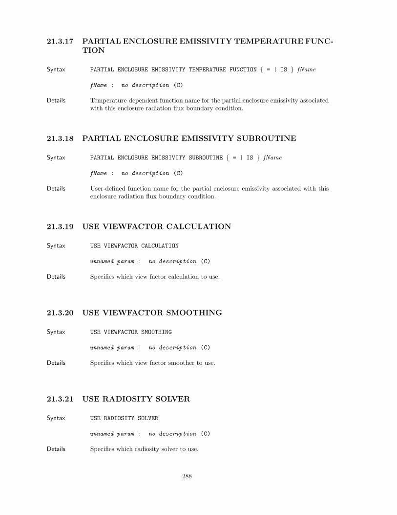
21.3.17 PARTIAL ENCLOSURE EMISSIVITY TEMPERATURE FUNC-TION
Syntax PARTIAL ENCLOSURE EMISSIVITY TEMPERATURE FUNCTION = | IS fName
fName : no description (C)
Details Temperature-dependent function name for the partial enclosure emissivity associatedwith this enclosure radiation flux boundary condition.
21.3.18 PARTIAL ENCLOSURE EMISSIVITY SUBROUTINE
Syntax PARTIAL ENCLOSURE EMISSIVITY SUBROUTINE = | IS fName
fName : no description (C)
Details User-defined function name for the partial enclosure emissivity associated with thisenclosure radiation flux boundary condition.
21.3.19 USE VIEWFACTOR CALCULATION
Syntax USE VIEWFACTOR CALCULATION
unnamed param : no description (C)
Details Specifies which view factor calculation to use.
21.3.20 USE VIEWFACTOR SMOOTHING
Syntax USE VIEWFACTOR SMOOTHING
unnamed param : no description (C)
Details Specifies which view factor smoother to use.
21.3.21 USE RADIOSITY SOLVER
Syntax USE RADIOSITY SOLVER
unnamed param : no description (C)
Details Specifies which radiosity solver to use.
288
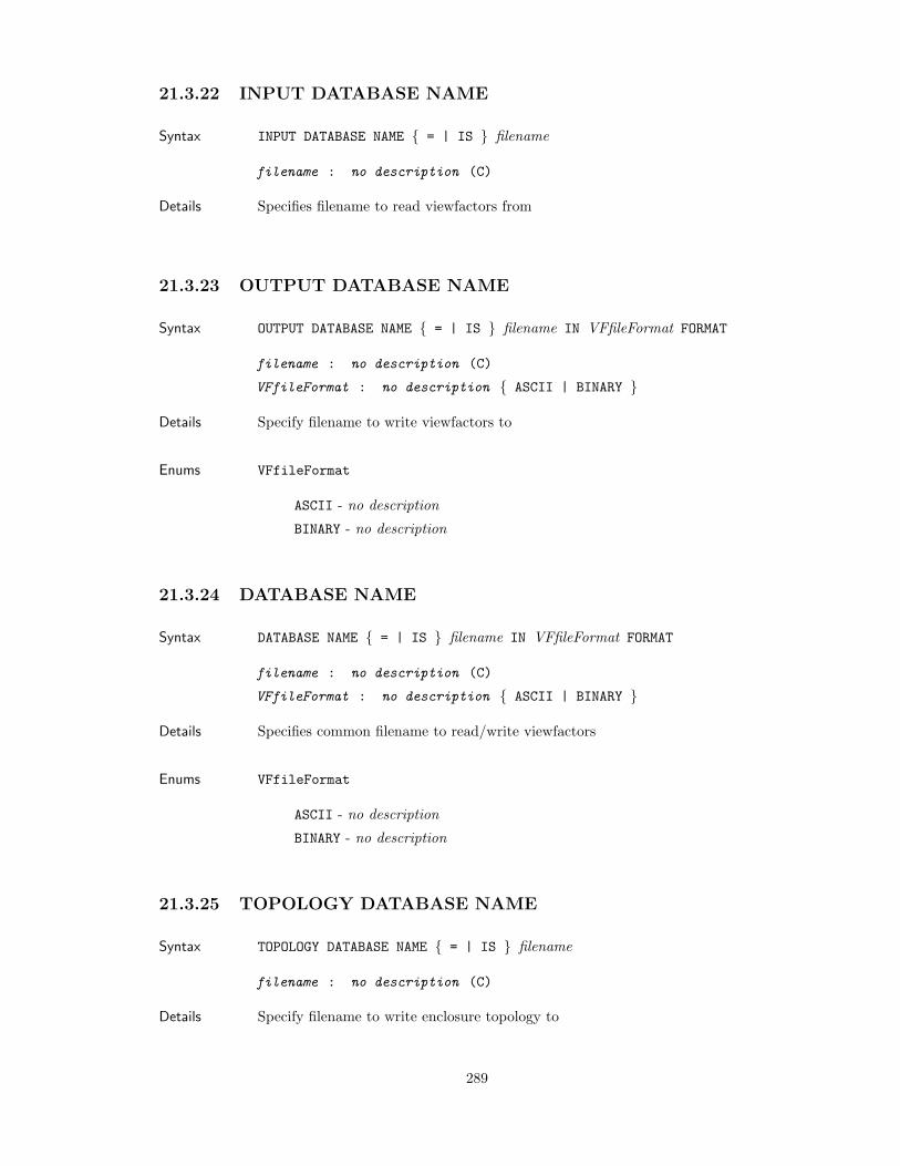
21.3.22 INPUT DATABASE NAME
Syntax INPUT DATABASE NAME = | IS filename
filename : no description (C)
Details Specifies filename to read viewfactors from
21.3.23 OUTPUT DATABASE NAME
Syntax OUTPUT DATABASE NAME = | IS filename IN VFfileFormat FORMAT
filename : no description (C)
VFfileFormat : no description ASCII | BINARY
Details Specify filename to write viewfactors to
Enums VFfileFormat
ASCII - no description
BINARY - no description
21.3.24 DATABASE NAME
Syntax DATABASE NAME = | IS filename IN VFfileFormat FORMAT
filename : no description (C)
VFfileFormat : no description ASCII | BINARY
Details Specifies common filename to read/write viewfactors
Enums VFfileFormat
ASCII - no description
BINARY - no description
21.3.25 TOPOLOGY DATABASE NAME
Syntax TOPOLOGY DATABASE NAME = | IS filename
filename : no description (C)
Details Specify filename to write enclosure topology to
289
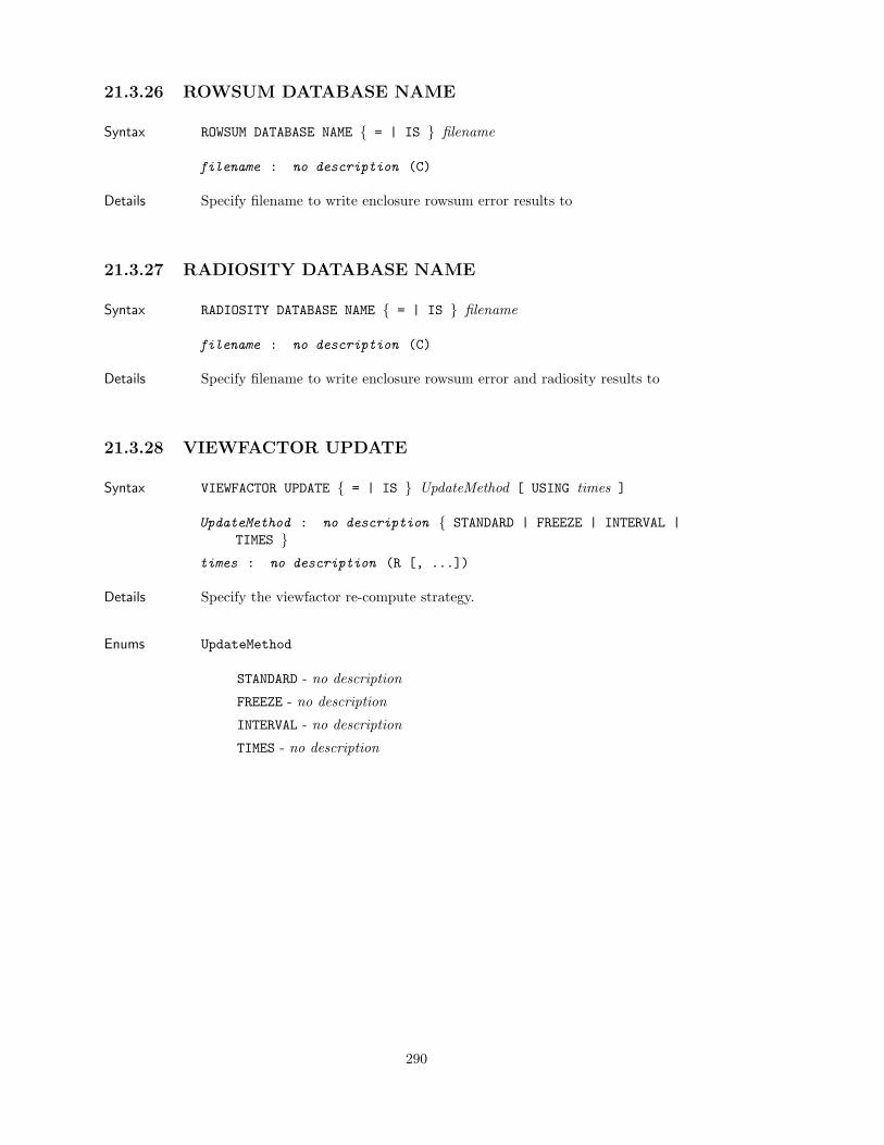
21.3.26 ROWSUM DATABASE NAME
Syntax ROWSUM DATABASE NAME = | IS filename
filename : no description (C)
Details Specify filename to write enclosure rowsum error results to
21.3.27 RADIOSITY DATABASE NAME
Syntax RADIOSITY DATABASE NAME = | IS filename
filename : no description (C)
Details Specify filename to write enclosure rowsum error and radiosity results to
21.3.28 VIEWFACTOR UPDATE
Syntax VIEWFACTOR UPDATE = | IS UpdateMethod [ USING times ]
UpdateMethod : no description STANDARD | FREEZE | INTERVAL |TIMES
times : no description (R [, ...])
Details Specify the viewfactor re-compute strategy.
Enums UpdateMethod
STANDARD - no description
FREEZE - no description
INTERVAL - no description
TIMES - no description
290
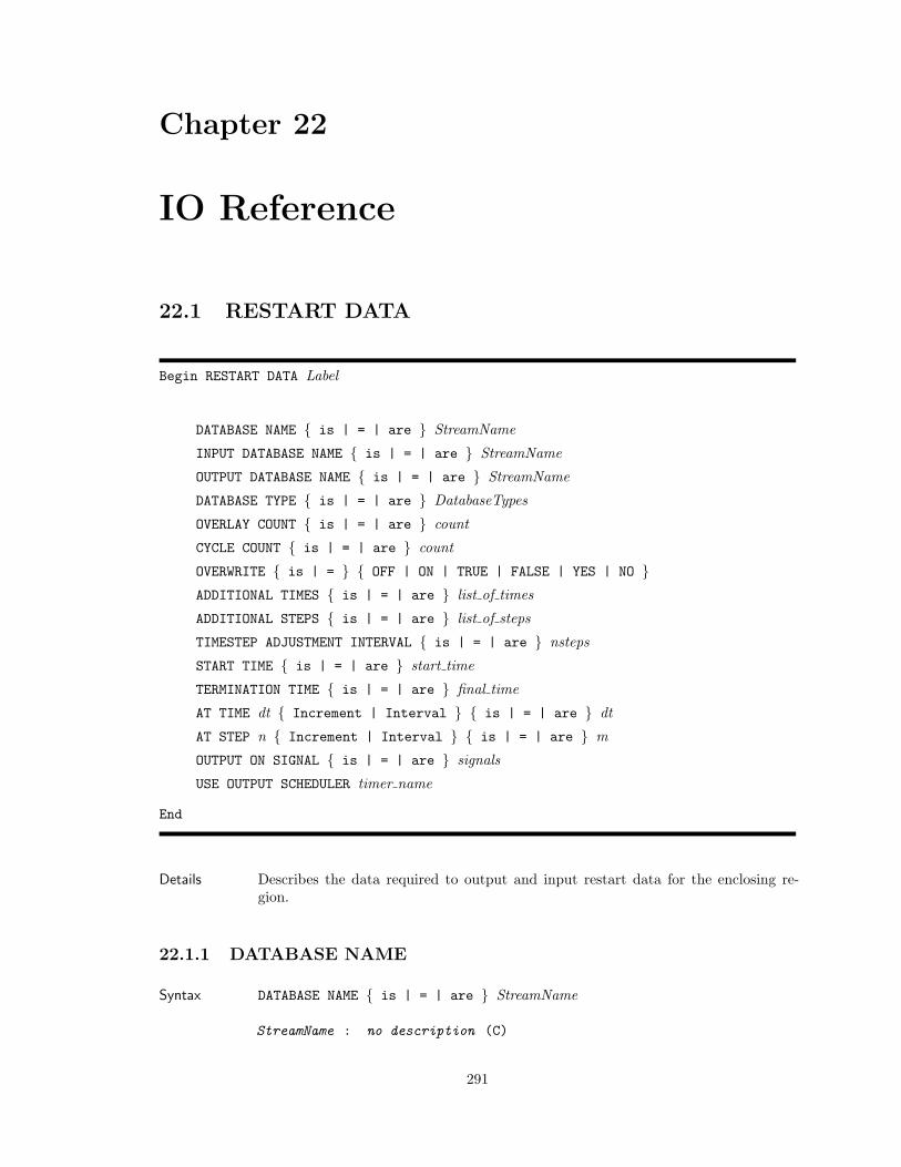
Chapter 22
IO Reference
22.1 RESTART DATA
Begin RESTART DATA Label
DATABASE NAME is | = | are StreamName
INPUT DATABASE NAME is | = | are StreamName
OUTPUT DATABASE NAME is | = | are StreamName
DATABASE TYPE is | = | are DatabaseTypes
OVERLAY COUNT is | = | are count
CYCLE COUNT is | = | are count
OVERWRITE is | = OFF | ON | TRUE | FALSE | YES | NO ADDITIONAL TIMES is | = | are list of times
ADDITIONAL STEPS is | = | are list of steps
TIMESTEP ADJUSTMENT INTERVAL is | = | are nsteps
START TIME is | = | are start time
TERMINATION TIME is | = | are final time
AT TIME dt Increment | Interval is | = | are dt
AT STEP n Increment | Interval is | = | are m
OUTPUT ON SIGNAL is | = | are signals
USE OUTPUT SCHEDULER timer name
End
Details Describes the data required to output and input restart data for the enclosing re-gion.
22.1.1 DATABASE NAME
Syntax DATABASE NAME is | = | are StreamName
StreamName : no description (C)
291
Details The database containing the input and/or output restart data. If this analysis isbeing restarted, restart data will be read from this file. If the analysis is writingrestart data, the data will be written to this file. It will be overwritten if it exists(after being read if applicable). If the filename begins with the ’/’ character, it is anabsolute path; otherwise, the path to the current directory will be prepended to thename. See also the ’Input Database’ and ’Output Database’ commands.
22.1.2 INPUT DATABASE NAME
Syntax INPUT DATABASE NAME is | = | are StreamName
StreamName : no description (C)
Details The database containing the input restart data. If this analysis is being restarted,restart data will be read from this file. See also the ’Database’ and ’Output Database’commands.
22.1.3 OUTPUT DATABASE NAME
Syntax OUTPUT DATABASE NAME is | = | are StreamName
StreamName : no description (C)
Details The database containing the output restart data. If the analysis is writing restartdata, the data will be written to this file. It will be overwritten if it exists. See alsothe ’Database’ and ’Input Database’ commands.
22.1.4 DATABASE TYPE
Syntax DATABASE TYPE is | = | are DatabaseTypes
DatabaseTypes : no description exodusII | SAF | xdmf
Details The database type/format used for the restart file.
Enums DatabaseTypes
exodusII - no description
SAF - no description
xdmf - no description
22.1.5 OVERLAY COUNT
Syntax OVERLAY COUNT is | = | are count
count : no description (I)
292
Details Specify the number of restart outputs which will be overlayed on top of the lastwritten step. For example, if restarts are being output every 0.1 seconds and theoverlay count is specified as 2, then restart will write times 0.1 to step 1 of thedatabase. It will then write 0.2 and 0.3 also to step 1. It will then increment thedatabase step and write 0.4 to step 2; overlay 0.5 and 0.6 on step 2... At the endof the analysis, assuming it runs to completion, the database would have times 0.3,0.6, 0.9, ... However, if there were a problem during the analysis, the last step on thedatabase would contain an intermediate step.
22.1.6 CYCLE COUNT
Syntax CYCLE COUNT is | = | are count
count : no description (I)
Details Specify the number of restart steps which will be written to the restart databasebefore previously written steps are overwritten. For example, if the cycle count is 5and restart is written every 0.1 seconds, the restart system will write 0.1, 0.2, 0.3,0.4, 0.5 to the database. It will then overwrite the first step with data from time 0.6,the second with time 0.7. At time 0.8, the database would contain data at times 0.6,0.7, 0.8, 0.4, 0.5. Note that time will not necessarily be monotonically increasing ona database that specifies the cycle count.
22.1.7 OVERWRITE
Details Specify whether the restart database should be overwritten if it exists. The defaultbehavior is to overwrite unless this command is specified in the restart block andeither off, false, or no is specified.
22.1.8 ADDITIONAL TIMES
Syntax ADDITIONAL TIMES is | = | are list of times
list of times : no description (R [, ...])
Details Additional simulation times when output should occur.
22.1.9 ADDITIONAL STEPS
Syntax ADDITIONAL STEPS is | = | are list of steps
list of steps : no description (I [, ...])
Details Additional simulation steps when output should occur.
293
22.1.10 TIMESTEP ADJUSTMENT INTERVAL
Syntax TIMESTEP ADJUSTMENT INTERVAL is | = | are nsteps
nsteps : no description (I)
Details Specify the number of steps to ’look ahead’ and adjust the timestep to ensure thatthe specified output times or simulation end time will be hit ’exactly’.
22.1.11 START TIME
Syntax START TIME is | = | are start time
start time : no description (R)
Details Specify the time to start outputting results from this output request block. This timeoverrides all ’at time’ and ’at step’ specifications.
22.1.12 TERMINATION TIME
Syntax TERMINATION TIME is | = | are final time
final time : no description (R)
Details Specify the time to stop outputting results from this output request block.
22.1.13 AT TIME
Syntax AT TIME dt Increment | Interval is | = | are dt
dt : no description (R)
dt : no description (R)
Details Specify an output interval in terms of the internal simulation time. The first timespecifies the time at the beginning of this time interval and the second time specifiesthe output frequency to be used within this interval.
22.1.14 AT STEP
Syntax AT STEP n Increment | Interval is | = | are m
n : no description (I)
m : no description (I)
294
Details Specify an output interval in terms of the internal iteration step count. The first stepspecifies the step count at the beginning of this interval and the second step specifiesthe output frequency to be used within this interval.
22.1.15 OUTPUT ON SIGNAL
Syntax OUTPUT ON SIGNAL is | = | are signals
signals : no description SIGALRM | SIGFPE | SIGHUP | SIGINT |SIGPIPE | SIGQUIT | SIGTERM | SIGUSR1 | SIGUSR2 | SIGABRT |SIGKILL | SIGILL | SIGSEGV
Details When the specified signal is raised, the output stream associated with this block willbe output.
Enums signals
SIGALRM - no description
SIGFPE - no description
SIGHUP - no description
SIGINT - no description
SIGPIPE - no description
SIGQUIT - no description
SIGTERM - no description
SIGUSR1 - no description
SIGUSR2 - no description
SIGABRT - no description
SIGKILL - no description
SIGILL - no description
SIGSEGV - no description
22.1.16 USE OUTPUT SCHEDULER
Syntax USE OUTPUT SCHEDULER timer name
timer name : no description (C)
Details Associates a predefined output scheduler with this output block (results, restart,heartbeat, or history).
22.2 RESULTS OUTPUT
Begin RESULTS OUTPUT Label
295
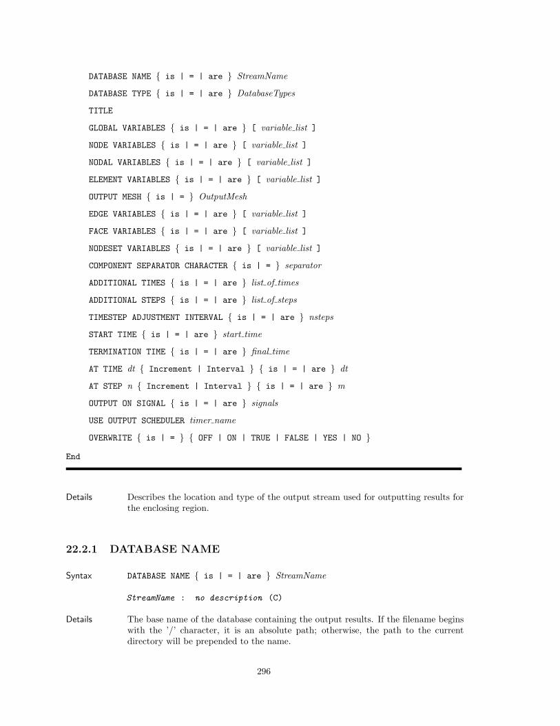
DATABASE NAME is | = | are StreamName
DATABASE TYPE is | = | are DatabaseTypes
TITLE
GLOBAL VARIABLES is | = | are [ variable list ]
NODE VARIABLES is | = | are [ variable list ]
NODAL VARIABLES is | = | are [ variable list ]
ELEMENT VARIABLES is | = | are [ variable list ]
OUTPUT MESH is | = OutputMesh
EDGE VARIABLES is | = | are [ variable list ]
FACE VARIABLES is | = | are [ variable list ]
NODESET VARIABLES is | = | are [ variable list ]
COMPONENT SEPARATOR CHARACTER is | = separator
ADDITIONAL TIMES is | = | are list of times
ADDITIONAL STEPS is | = | are list of steps
TIMESTEP ADJUSTMENT INTERVAL is | = | are nsteps
START TIME is | = | are start time
TERMINATION TIME is | = | are final time
AT TIME dt Increment | Interval is | = | are dt
AT STEP n Increment | Interval is | = | are m
OUTPUT ON SIGNAL is | = | are signals
USE OUTPUT SCHEDULER timer name
OVERWRITE is | = OFF | ON | TRUE | FALSE | YES | NO
End
Details Describes the location and type of the output stream used for outputting results forthe enclosing region.
22.2.1 DATABASE NAME
Syntax DATABASE NAME is | = | are StreamName
StreamName : no description (C)
Details The base name of the database containing the output results. If the filename beginswith the ’/’ character, it is an absolute path; otherwise, the path to the currentdirectory will be prepended to the name.
296
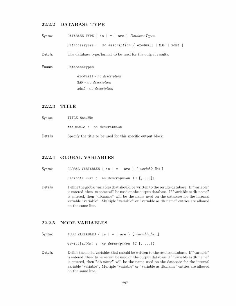
22.2.2 DATABASE TYPE
Syntax DATABASE TYPE is | = | are DatabaseTypes
DatabaseTypes : no description exodusII | SAF | xdmf
Details The database type/format to be used for the output results.
Enums DatabaseTypes
exodusII - no description
SAF - no description
xdmf - no description
22.2.3 TITLE
Syntax TITLE the title
the title : no description
Details Specify the title to be used for this specific output block.
22.2.4 GLOBAL VARIABLES
Syntax GLOBAL VARIABLES is | = | are [ variable list ]
variable list : no description (C [, ...])
Details Define the global variables that should be written to the results database. If ”variable”is entered, then its name will be used on the output database. If ”variable as db name”is entered, then ”db name” will be the name used on the database for the internalvariable ”variable”. Multiple ”variable” or ”variable as db name” entries are allowedon the same line.
22.2.5 NODE VARIABLES
Syntax NODE VARIABLES is | = | are [ variable list ]
variable list : no description (C [, ...])
Details Define the nodal variables that should be written to the results database. If ”variable”is entered, then its name will be used on the output database. If ”variable as db name”is entered, then ”db name” will be the name used on the database for the internalvariable ”variable”. Multiple ”variable” or ”variable as db name” entries are allowedon the same line.
297
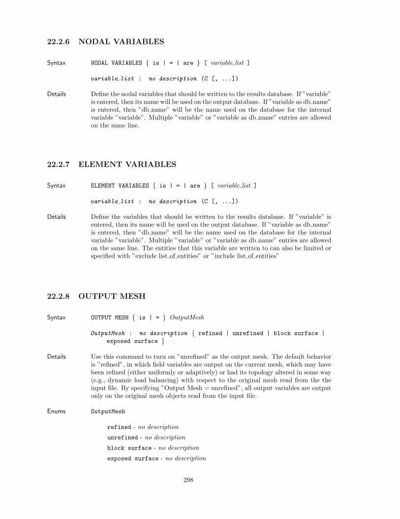
22.2.6 NODAL VARIABLES
Syntax NODAL VARIABLES is | = | are [ variable list ]
variable list : no description (C [, ...])
Details Define the nodal variables that should be written to the results database. If ”variable”is entered, then its name will be used on the output database. If ”variable as db name”is entered, then ”db name” will be the name used on the database for the internalvariable ”variable”. Multiple ”variable” or ”variable as db name” entries are allowedon the same line.
22.2.7 ELEMENT VARIABLES
Syntax ELEMENT VARIABLES is | = | are [ variable list ]
variable list : no description (C [, ...])
Details Define the variables that should be written to the results database. If ”variable” isentered, then its name will be used on the output database. If ”variable as db name”is entered, then ”db name” will be the name used on the database for the internalvariable ”variable”. Multiple ”variable” or ”variable as db name” entries are allowedon the same line. The entities that this variable are written to can also be limited orspecified with ”exclude list of entities” or ”include list of entities”
22.2.8 OUTPUT MESH
Syntax OUTPUT MESH is | = OutputMesh
OutputMesh : no description refined | unrefined | block surface |exposed surface
Details Use this command to turn on ”unrefined” as the output mesh. The default behavioris ”refined”, in which field variables are output on the current mesh, which may havebeen refined (either uniformly or adaptively) or had its topology altered in some way(e.g., dynamic load balancing) with respect to the original mesh read from the theinput file. By specifying ”Output Mesh = unrefined”, all output variables are outputonly on the original mesh objects read from the input file.
Enums OutputMesh
refined - no description
unrefined - no description
block surface - no description
exposed surface - no description
298

22.2.9 EDGE VARIABLES
Syntax EDGE VARIABLES is | = | are [ variable list ]
variable list : no description (C [, ...])
Details Define the variables that should be written to the results database. If ”variable” isentered, then its name will be used on the output database. If ”variable as db name”is entered, then ”db name” will be the name used on the database for the internalvariable ”variable”. Multiple ”variable” or ”variable as db name” entries are allowedon the same line. The entities that this variable are written to can also be limitedor specified with ”exclude list of entities” or ”include list of entities”. Edge variablesare not supported for all database types.
22.2.10 FACE VARIABLES
Syntax FACE VARIABLES is | = | are [ variable list ]
variable list : no description (C [, ...])
Details Define the variables that should be written to the results database. If ”variable” isentered, then its name will be used on the output database. If ”variable as db name”is entered, then ”db name” will be the name used on the database for the internalvariable ”variable”. Multiple ”variable” or ”variable as db name” entries are allowedon the same line. The entities that this variable are written to can also be limitedor specified with ”exclude list of entities” or ”include list of entities”. Face variablesare not supported for all database types.
22.2.11 NODESET VARIABLES
Syntax NODESET VARIABLES is | = | are [ variable list ]
variable list : no description (C [, ...])
Details Define the variables that should be written to the results database. If ”variable” isentered, then its name will be used on the output database. If ”variable as db name”is entered, then ”db name” will be the name used on the database for the internalvariable ”variable”. Multiple ”variable” or ”variable as db name” entries are allowedon the same line. The entities that this variable are written to can also be limited orspecified with ”exclude list of entities” or ”include list of entities”. Nodeset variablesare not supported for all database types.
22.2.12 COMPONENT SEPARATOR CHARACTER
Syntax COMPONENT SEPARATOR CHARACTER is | = separator
separator : no description (C)
299

Details The separator is the single character used to separate the output variable basename(e.g. ”stress”) from the suffices (e.g. ”xx”, ”yy”) when displaying the names of theindividual variable components. For example, the default separator is ” ”, whichresults in names similar to ”stress xx”, ”stress yy”, ... ”stress zx”. To eliminate theseparator, specify an empty string (””) or NONE.
22.2.13 ADDITIONAL TIMES
Syntax ADDITIONAL TIMES is | = | are list of times
list of times : no description (R [, ...])
Details Additional simulation times when output should occur.
22.2.14 ADDITIONAL STEPS
Syntax ADDITIONAL STEPS is | = | are list of steps
list of steps : no description (I [, ...])
Details Additional simulation steps when output should occur.
22.2.15 TIMESTEP ADJUSTMENT INTERVAL
Syntax TIMESTEP ADJUSTMENT INTERVAL is | = | are nsteps
nsteps : no description (I)
Details Specify the number of steps to ’look ahead’ and adjust the timestep to ensure thatthe specified output times or simulation end time will be hit ’exactly’.
22.2.16 START TIME
Syntax START TIME is | = | are start time
start time : no description (R)
Details Specify the time to start outputting results from this output request block. This timeoverrides all ’at time’ and ’at step’ specifications.
22.2.17 TERMINATION TIME
Syntax TERMINATION TIME is | = | are final time
final time : no description (R)
300
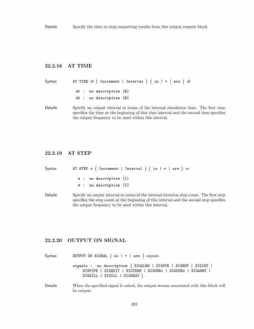
Details Specify the time to stop outputting results from this output request block.
22.2.18 AT TIME
Syntax AT TIME dt Increment | Interval is | = | are dt
dt : no description (R)
dt : no description (R)
Details Specify an output interval in terms of the internal simulation time. The first timespecifies the time at the beginning of this time interval and the second time specifiesthe output frequency to be used within this interval.
22.2.19 AT STEP
Syntax AT STEP n Increment | Interval is | = | are m
n : no description (I)
m : no description (I)
Details Specify an output interval in terms of the internal iteration step count. The first stepspecifies the step count at the beginning of this interval and the second step specifiesthe output frequency to be used within this interval.
22.2.20 OUTPUT ON SIGNAL
Syntax OUTPUT ON SIGNAL is | = | are signals
signals : no description SIGALRM | SIGFPE | SIGHUP | SIGINT |SIGPIPE | SIGQUIT | SIGTERM | SIGUSR1 | SIGUSR2 | SIGABRT |SIGKILL | SIGILL | SIGSEGV
Details When the specified signal is raised, the output stream associated with this block willbe output.
301
Enums signals
SIGALRM - no description
SIGFPE - no description
SIGHUP - no description
SIGINT - no description
SIGPIPE - no description
SIGQUIT - no description
SIGTERM - no description
SIGUSR1 - no description
SIGUSR2 - no description
SIGABRT - no description
SIGKILL - no description
SIGILL - no description
SIGSEGV - no description
22.2.21 USE OUTPUT SCHEDULER
Syntax USE OUTPUT SCHEDULER timer name
timer name : no description (C)
Details Associates a predefined output scheduler with this output block (results, restart,heartbeat, or history).
22.2.22 OVERWRITE
Details Specify whether the database should be overwritten if it exists. The default behavioris to overwrite unless this command is specified in the output block and either off,false, or no is specified.
22.3 HEARTBEAT
Begin HEARTBEAT Label
ADDITIONAL TIMES is | = | are list of times
ADDITIONAL STEPS is | = | are list of steps
TIMESTEP ADJUSTMENT INTERVAL is | = | are nsteps
START TIME is | = | are start time
TERMINATION TIME is | = | are final time
AT TIME dt Increment | Interval is | = | are dt
302
AT STEP n Increment | Interval is | = | are m
OUTPUT ON SIGNAL is | = | are signals
USE OUTPUT SCHEDULER timer name
STREAM NAME is | = | are StreamName
PRECISION is | = | are precision
LABELS is | = | are on | off
MONITOR is | = | are | the results | restart | history
TIMESTAMP FORMAT
LEGEND is | = | are on | off
VARIABLE is | = | are global | node | nodal | element | face | edge [ vari-able list ]
End
Details Describes the location and type of the output stream used for outputting the heart-beat information for the enclosing region.
22.3.1 ADDITIONAL TIMES
Syntax ADDITIONAL TIMES is | = | are list of times
list of times : no description (R [, ...])
Details Additional simulation times when output should occur.
22.3.2 ADDITIONAL STEPS
Syntax ADDITIONAL STEPS is | = | are list of steps
list of steps : no description (I [, ...])
Details Additional simulation steps when output should occur.
22.3.3 TIMESTEP ADJUSTMENT INTERVAL
Syntax TIMESTEP ADJUSTMENT INTERVAL is | = | are nsteps
nsteps : no description (I)
Details Specify the number of steps to ’look ahead’ and adjust the timestep to ensure thatthe specified output times or simulation end time will be hit ’exactly’.
303
22.3.4 START TIME
Syntax START TIME is | = | are start time
start time : no description (R)
Details Specify the time to start outputting results from this output request block. This timeoverrides all ’at time’ and ’at step’ specifications.
22.3.5 TERMINATION TIME
Syntax TERMINATION TIME is | = | are final time
final time : no description (R)
Details Specify the time to stop outputting results from this output request block.
22.3.6 AT TIME
Syntax AT TIME dt Increment | Interval is | = | are dt
dt : no description (R)
dt : no description (R)
Details Specify an output interval in terms of the internal simulation time. The first timespecifies the time at the beginning of this time interval and the second time specifiesthe output frequency to be used within this interval.
22.3.7 AT STEP
Syntax AT STEP n Increment | Interval is | = | are m
n : no description (I)
m : no description (I)
Details Specify an output interval in terms of the internal iteration step count. The first stepspecifies the step count at the beginning of this interval and the second step specifiesthe output frequency to be used within this interval.
22.3.8 OUTPUT ON SIGNAL
Syntax OUTPUT ON SIGNAL is | = | are signals
signals : no description SIGALRM | SIGFPE | SIGHUP | SIGINT |SIGPIPE | SIGQUIT | SIGTERM | SIGUSR1 | SIGUSR2 | SIGABRT |SIGKILL | SIGILL | SIGSEGV
304
Details When the specified signal is raised, the output stream associated with this block willbe output.
Enums signals
SIGALRM - no description
SIGFPE - no description
SIGHUP - no description
SIGINT - no description
SIGPIPE - no description
SIGQUIT - no description
SIGTERM - no description
SIGUSR1 - no description
SIGUSR2 - no description
SIGABRT - no description
SIGKILL - no description
SIGILL - no description
SIGSEGV - no description
22.3.9 USE OUTPUT SCHEDULER
Syntax USE OUTPUT SCHEDULER timer name
timer name : no description (C)
Details Associates a predefined output scheduler with this output block (results, restart,heartbeat, or history).
22.3.10 STREAM NAME
Syntax STREAM NAME is | = | are StreamName
StreamName : no description (C)
Details The base name of the stream containing the output results. If the filename beginswith the ’/’ character, it is an absolute path; otherwise, the path to the currentdirectory will be prepended to the name. In addition, there are several predefinedstreams that can be specified. The predefined streams are ’cout’ or ’stdout’ specifiesstandard output; ’cerr’, ’stderr’, ’clog’, or ’log’ specifies standard error; ’output’ or’outputP0’ specifies Sierra’s standard output which is redirected to the file specifiedby the ’-o’ option on the command line. If the file already exists, it is overwritten.
305
22.3.11 PRECISION
Syntax PRECISION is | = | are precision
precision : no description (I)
Details The precsion to be used for the output of real variables.
22.3.12 LABELS
Details Specifies whether labels will be displayed or just the value of the variable. Labels willbe shown if this line is not present.
22.3.13 MONITOR
Details Specifies whether a line will be written to the heartbeat stream when either theresults, history, and/or restart data are output.
22.3.14 TIMESTAMP FORMAT
Syntax TIMESTAMP FORMAT FormatString
FormatString : no description
Details The format to be used for the timestamp. See ’man strftime’ for more information.
22.3.15 LEGEND
Details Specifies whether a legend will be displayed prior to outputting any variables. Thelegend will not be shown unless this line is present. The legend shows the namesof the variables that will be written to the heartbeat output stream. If the variablehas multiple components, then the component count is shown after the variable e.g.,velocity(3).
22.3.16 VARIABLE
Syntax VARIABLE is | = | are global | node | nodal | element | face |edge [ variable list ]
variable list : no description (C [, ...])
306
Details Define the variables that should be written to the heartbeat output. The user canrequest that the values of certain variables be output on the heartbeat line. Thesevariables are limited to region and framework control data currently. The syntax is:
variable = entity_type internal_name atentity_type entity_id as external_name
variable = entity_type internal_name nearest locationx,y,z as external_name
For global variables, use:
variable = global internal_name [as external_name]
Where:
entity_type = node, element, face, edge, globalinternal_name = Sierra variable nameentity_id = id of the node, element, face, edge that you want
the specified variable output at.external_name = name of variable on the database.
The names ’timestep’, and ’time’ can be specified as variables also. They are thecurrent timestep and simulation time. This line can appear multiple times.
22.4 HISTORY OUTPUT
Begin HISTORY OUTPUT Label
ADDITIONAL TIMES is | = | are list of times
ADDITIONAL STEPS is | = | are list of steps
TIMESTEP ADJUSTMENT INTERVAL is | = | are nsteps
START TIME is | = | are start time
TERMINATION TIME is | = | are final time
AT TIME dt Increment | Interval is | = | are dt
AT STEP n Increment | Interval is | = | are m
OUTPUT ON SIGNAL is | = | are signals
USE OUTPUT SCHEDULER timer name
OVERWRITE is | = OFF | ON | TRUE | FALSE | YES | NO DATABASE NAME is | = | are StreamName
DATABASE TYPE is | = | are DatabaseTypes
TITLE
307
VARIABLE is | = | are global | node | nodal | element | face | edge [ vari-able list ]
End
Details Describes the location and type of the output stream used for outputting history forthe enclosing region.
22.4.1 ADDITIONAL TIMES
Syntax ADDITIONAL TIMES is | = | are list of times
list of times : no description (R [, ...])
Details Additional simulation times when output should occur.
22.4.2 ADDITIONAL STEPS
Syntax ADDITIONAL STEPS is | = | are list of steps
list of steps : no description (I [, ...])
Details Additional simulation steps when output should occur.
22.4.3 TIMESTEP ADJUSTMENT INTERVAL
Syntax TIMESTEP ADJUSTMENT INTERVAL is | = | are nsteps
nsteps : no description (I)
Details Specify the number of steps to ’look ahead’ and adjust the timestep to ensure thatthe specified output times or simulation end time will be hit ’exactly’.
22.4.4 START TIME
Syntax START TIME is | = | are start time
start time : no description (R)
Details Specify the time to start outputting results from this output request block. This timeoverrides all ’at time’ and ’at step’ specifications.
308
22.4.5 TERMINATION TIME
Syntax TERMINATION TIME is | = | are final time
final time : no description (R)
Details Specify the time to stop outputting results from this output request block.
22.4.6 AT TIME
Syntax AT TIME dt Increment | Interval is | = | are dt
dt : no description (R)
dt : no description (R)
Details Specify an output interval in terms of the internal simulation time. The first timespecifies the time at the beginning of this time interval and the second time specifiesthe output frequency to be used within this interval.
22.4.7 AT STEP
Syntax AT STEP n Increment | Interval is | = | are m
n : no description (I)
m : no description (I)
Details Specify an output interval in terms of the internal iteration step count. The first stepspecifies the step count at the beginning of this interval and the second step specifiesthe output frequency to be used within this interval.
22.4.8 OUTPUT ON SIGNAL
Syntax OUTPUT ON SIGNAL is | = | are signals
signals : no description SIGALRM | SIGFPE | SIGHUP | SIGINT |SIGPIPE | SIGQUIT | SIGTERM | SIGUSR1 | SIGUSR2 | SIGABRT |SIGKILL | SIGILL | SIGSEGV
Details When the specified signal is raised, the output stream associated with this block willbe output.
309
Enums signals
SIGALRM - no description
SIGFPE - no description
SIGHUP - no description
SIGINT - no description
SIGPIPE - no description
SIGQUIT - no description
SIGTERM - no description
SIGUSR1 - no description
SIGUSR2 - no description
SIGABRT - no description
SIGKILL - no description
SIGILL - no description
SIGSEGV - no description
22.4.9 USE OUTPUT SCHEDULER
Syntax USE OUTPUT SCHEDULER timer name
timer name : no description (C)
Details Associates a predefined output scheduler with this output block (results, restart,heartbeat, or history).
22.4.10 OVERWRITE
Details Specify whether the database should be overwritten if it exists. The default behavioris to overwrite unless this command is specified in the output block and either off,false, or no is specified.
22.4.11 DATABASE NAME
Syntax DATABASE NAME is | = | are StreamName
StreamName : no description (C)
Details The base name of the database containing the output history. If the filename beginswith the ’/’ character, it is an absolute path; otherwise, the path to the currentdirectory will be prepended to the name.
310
22.4.12 DATABASE TYPE
Syntax DATABASE TYPE is | = | are DatabaseTypes
DatabaseTypes : no description exodusII | SAF | xdmf
Details The database type/format to be used for the output history.
Enums DatabaseTypes
exodusII - no description
SAF - no description
xdmf - no description
22.4.13 TITLE
Syntax TITLE the title
the title : no description
Details Specify the title to be used for this specific output block.
22.4.14 VARIABLE
Syntax VARIABLE is | = | are global | node | nodal | element | face |edge [ variable list ]
variable list : no description (C [, ...])
Details Define the variables that should be written to the history database. The syntax is:
variable = entity internal_name at entity id as DBname
or
variable = entity internal_name nearest location X, Y, Z as DBname
or
variable = entity internal_name at location X, Y, Z as DBname.
Where entity is ’node’, ’element’, ’face’, or ’edge’; internal name is the name ofthe variable in the Sierra application; and DBname is the name as it should appearon the history database.
311

22.5 RESULTS OUTPUT
Begin RESULTS OUTPUT Label
DATABASE NAME is | = | are StreamName
DATABASE TYPE is | = | are DatabaseTypes
TITLE
GLOBAL VARIABLES is | = | are [ variable list ]
NODE VARIABLES is | = | are [ variable list ]
NODAL VARIABLES is | = | are [ variable list ]
ELEMENT VARIABLES is | = | are [ variable list ]
OUTPUT MESH is | = OutputMesh
EDGE VARIABLES is | = | are [ variable list ]
FACE VARIABLES is | = | are [ variable list ]
NODESET VARIABLES is | = | are [ variable list ]
COMPONENT SEPARATOR CHARACTER is | = separator
ADDITIONAL TIMES is | = | are list of times
ADDITIONAL STEPS is | = | are list of steps
TIMESTEP ADJUSTMENT INTERVAL is | = | are nsteps
START TIME is | = | are start time
TERMINATION TIME is | = | are final time
AT TIME dt Increment | Interval is | = | are dt
AT STEP n Increment | Interval is | = | are m
OUTPUT ON SIGNAL is | = | are signals
USE OUTPUT SCHEDULER timer name
OVERWRITE is | = OFF | ON | TRUE | FALSE | YES | NO
End
Details Describes the location and type of the output stream used for outputting results forthe enclosing region.
22.5.1 DATABASE NAME
Syntax DATABASE NAME is | = | are StreamName
StreamName : no description (C)
Details The base name of the database containing the output results. If the filename beginswith the ’/’ character, it is an absolute path; otherwise, the path to the currentdirectory will be prepended to the name.
312

22.5.2 DATABASE TYPE
Syntax DATABASE TYPE is | = | are DatabaseTypes
DatabaseTypes : no description exodusII | SAF | xdmf
Details The database type/format to be used for the output results.
Enums DatabaseTypes
exodusII - no description
SAF - no description
xdmf - no description
22.5.3 TITLE
Syntax TITLE the title
the title : no description
Details Specify the title to be used for this specific output block.
22.5.4 GLOBAL VARIABLES
Syntax GLOBAL VARIABLES is | = | are [ variable list ]
variable list : no description (C [, ...])
Details Define the global variables that should be written to the results database. If ”variable”is entered, then its name will be used on the output database. If ”variable as db name”is entered, then ”db name” will be the name used on the database for the internalvariable ”variable”. Multiple ”variable” or ”variable as db name” entries are allowedon the same line.
22.5.5 NODE VARIABLES
Syntax NODE VARIABLES is | = | are [ variable list ]
variable list : no description (C [, ...])
Details Define the nodal variables that should be written to the results database. If ”variable”is entered, then its name will be used on the output database. If ”variable as db name”is entered, then ”db name” will be the name used on the database for the internalvariable ”variable”. Multiple ”variable” or ”variable as db name” entries are allowedon the same line.
313

22.5.6 NODAL VARIABLES
Syntax NODAL VARIABLES is | = | are [ variable list ]
variable list : no description (C [, ...])
Details Define the nodal variables that should be written to the results database. If ”variable”is entered, then its name will be used on the output database. If ”variable as db name”is entered, then ”db name” will be the name used on the database for the internalvariable ”variable”. Multiple ”variable” or ”variable as db name” entries are allowedon the same line.
22.5.7 ELEMENT VARIABLES
Syntax ELEMENT VARIABLES is | = | are [ variable list ]
variable list : no description (C [, ...])
Details Define the variables that should be written to the results database. If ”variable” isentered, then its name will be used on the output database. If ”variable as db name”is entered, then ”db name” will be the name used on the database for the internalvariable ”variable”. Multiple ”variable” or ”variable as db name” entries are allowedon the same line. The entities that this variable are written to can also be limited orspecified with ”exclude list of entities” or ”include list of entities”
22.5.8 OUTPUT MESH
Syntax OUTPUT MESH is | = OutputMesh
OutputMesh : no description refined | unrefined | block surface |exposed surface
Details Use this command to turn on ”unrefined” as the output mesh. The default behavioris ”refined”, in which field variables are output on the current mesh, which may havebeen refined (either uniformly or adaptively) or had its topology altered in some way(e.g., dynamic load balancing) with respect to the original mesh read from the theinput file. By specifying ”Output Mesh = unrefined”, all output variables are outputonly on the original mesh objects read from the input file.
Enums OutputMesh
refined - no description
unrefined - no description
block surface - no description
exposed surface - no description
314
22.5.9 EDGE VARIABLES
Syntax EDGE VARIABLES is | = | are [ variable list ]
variable list : no description (C [, ...])
Details Define the variables that should be written to the results database. If ”variable” isentered, then its name will be used on the output database. If ”variable as db name”is entered, then ”db name” will be the name used on the database for the internalvariable ”variable”. Multiple ”variable” or ”variable as db name” entries are allowedon the same line. The entities that this variable are written to can also be limitedor specified with ”exclude list of entities” or ”include list of entities”. Edge variablesare not supported for all database types.
22.5.10 FACE VARIABLES
Syntax FACE VARIABLES is | = | are [ variable list ]
variable list : no description (C [, ...])
Details Define the variables that should be written to the results database. If ”variable” isentered, then its name will be used on the output database. If ”variable as db name”is entered, then ”db name” will be the name used on the database for the internalvariable ”variable”. Multiple ”variable” or ”variable as db name” entries are allowedon the same line. The entities that this variable are written to can also be limitedor specified with ”exclude list of entities” or ”include list of entities”. Face variablesare not supported for all database types.
22.5.11 NODESET VARIABLES
Syntax NODESET VARIABLES is | = | are [ variable list ]
variable list : no description (C [, ...])
Details Define the variables that should be written to the results database. If ”variable” isentered, then its name will be used on the output database. If ”variable as db name”is entered, then ”db name” will be the name used on the database for the internalvariable ”variable”. Multiple ”variable” or ”variable as db name” entries are allowedon the same line. The entities that this variable are written to can also be limited orspecified with ”exclude list of entities” or ”include list of entities”. Nodeset variablesare not supported for all database types.
22.5.12 COMPONENT SEPARATOR CHARACTER
Syntax COMPONENT SEPARATOR CHARACTER is | = separator
separator : no description (C)
315
Details The separator is the single character used to separate the output variable basename(e.g. ”stress”) from the suffices (e.g. ”xx”, ”yy”) when displaying the names of theindividual variable components. For example, the default separator is ” ”, whichresults in names similar to ”stress xx”, ”stress yy”, ... ”stress zx”. To eliminate theseparator, specify an empty string (””) or NONE.
22.5.13 ADDITIONAL TIMES
Syntax ADDITIONAL TIMES is | = | are list of times
list of times : no description (R [, ...])
Details Additional simulation times when output should occur.
22.5.14 ADDITIONAL STEPS
Syntax ADDITIONAL STEPS is | = | are list of steps
list of steps : no description (I [, ...])
Details Additional simulation steps when output should occur.
22.5.15 TIMESTEP ADJUSTMENT INTERVAL
Syntax TIMESTEP ADJUSTMENT INTERVAL is | = | are nsteps
nsteps : no description (I)
Details Specify the number of steps to ’look ahead’ and adjust the timestep to ensure thatthe specified output times or simulation end time will be hit ’exactly’.
22.5.16 START TIME
Syntax START TIME is | = | are start time
start time : no description (R)
Details Specify the time to start outputting results from this output request block. This timeoverrides all ’at time’ and ’at step’ specifications.
22.5.17 TERMINATION TIME
Syntax TERMINATION TIME is | = | are final time
final time : no description (R)
316

Details Specify the time to stop outputting results from this output request block.
22.5.18 AT TIME
Syntax AT TIME dt Increment | Interval is | = | are dt
dt : no description (R)
dt : no description (R)
Details Specify an output interval in terms of the internal simulation time. The first timespecifies the time at the beginning of this time interval and the second time specifiesthe output frequency to be used within this interval.
22.5.19 AT STEP
Syntax AT STEP n Increment | Interval is | = | are m
n : no description (I)
m : no description (I)
Details Specify an output interval in terms of the internal iteration step count. The first stepspecifies the step count at the beginning of this interval and the second step specifiesthe output frequency to be used within this interval.
22.5.20 OUTPUT ON SIGNAL
Syntax OUTPUT ON SIGNAL is | = | are signals
signals : no description SIGALRM | SIGFPE | SIGHUP | SIGINT |SIGPIPE | SIGQUIT | SIGTERM | SIGUSR1 | SIGUSR2 | SIGABRT |SIGKILL | SIGILL | SIGSEGV
Details When the specified signal is raised, the output stream associated with this block willbe output.
317
Enums signals
SIGALRM - no description
SIGFPE - no description
SIGHUP - no description
SIGINT - no description
SIGPIPE - no description
SIGQUIT - no description
SIGTERM - no description
SIGUSR1 - no description
SIGUSR2 - no description
SIGABRT - no description
SIGKILL - no description
SIGILL - no description
SIGSEGV - no description
22.5.21 USE OUTPUT SCHEDULER
Syntax USE OUTPUT SCHEDULER timer name
timer name : no description (C)
Details Associates a predefined output scheduler with this output block (results, restart,heartbeat, or history).
22.5.22 OVERWRITE
Details Specify whether the database should be overwritten if it exists. The default behavioris to overwrite unless this command is specified in the output block and either off,false, or no is specified.
22.6 PARAMETERS FOR BLOCK
Begin PARAMETERS FOR BLOCK Blockname
ACTIVE FOR PROCEDURE procedureName during periods periodNames
INACTIVE FOR PROCEDURE procedureName during periods periodNames
MATERIAL MatName
PHASE Phase Label = | IS | ARE Material Name
DEACTIVATE CodeName
SHELL INTEGRATION POINTS = | IS | ARE npoints
318
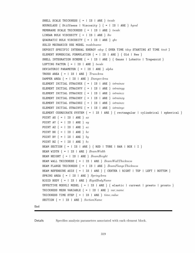
SHELL SCALE THICKNESS = | IS | ARE tscaleHOURGLASS Stiffness | Viscosity = | IS | ARE hgvalMEMBRANE SCALE THICKNESS = | IS | ARE tscaleLINEAR BULK VISCOSITY = | IS | ARE lbvQUADRATIC BULK VISCOSITY = | IS | ARE qbvSOLID MECHANICS USE MODEL modelnameDEPOSIT SPECIFIC INTERNAL ENERGY edep [ OVER TIME tdep STARTING AT TIME tinit ]
ELEMENT NUMERICAL FORMULATION = | IS | ARE Old | New SHELL INTEGRATION SCHEME = | IS | ARE Gauss | Lobatto | Trapezoid LOFTING FACTOR = | IS | ARE tscaleDEVIATORIC PARAMETER = | IS | ARE alphaTRUSS AREA = | IS | ARE TrussAreaDAMPER AREA = | IS | ARE DamperAreaELEMENT INITIAL STRAINXX = | IS | ARE istrainxxELEMENT INITIAL STRAINYY = | IS | ARE istrainyyELEMENT INITIAL STRAINZZ = | IS | ARE istrainzzELEMENT INITIAL STRAINXY = | IS | ARE istrainxyELEMENT INITIAL STRAINXZ = | IS | ARE istrainxzELEMENT INITIAL STRAINYZ = | IS | ARE istrainyzELEMENT COORDINATE SYSTEM = | IS | ARE rectangular | cylindrical | spherical POINT AX = | IS | ARE axPOINT AY = | IS | ARE ayPOINT AZ = | IS | ARE azPOINT BX = | IS | ARE bxPOINT BY = | IS | ARE byPOINT BZ = | IS | ARE bzBEAM SECTION = | IS | ARE ROD | TUBE | BAR | BOX | I BEAM WIDTH = | IS | ARE BeamWidthBEAM HEIGHT = | IS | ARE BeamHeightBEAM WALL THICKNESS = | IS | ARE BeamWallThicknessBEAM FLANGE THICKNESS = | IS | ARE BeamFlangeThicknessBEAM REFERECNE AXIS = | IS | ARE CENTER | RIGHT | TOP | LEFT | BOTTOM SPRING AREA = | IS | ARE SpringAreaRIGID BODY = | IS | ARE RigidBodyNameEFFECTIVE MODULI MODEL = | IS | ARE elastic | current | presto | pronto THICKNESS MESH VARIABLE = | IS | ARE var nameTHICKNESS TIME STEP = | IS | ARE time valueSECTION = | IS | ARE SectionName
End
Details Specifies analysis parameters associated with each element block.
319
22.6.1 ACTIVE FOR PROCEDURE
Syntax ACTIVE FOR PROCEDURE procedureName during periods periodNames
procedureName : no description (C)
periodNames : no description (C [, ...])
Details Lists the solution periods during which the given BC, solver, preconditioner, etc. isactive. Multiple uses of this line command within a single block will have a cumulativeaffect.
22.6.2 INACTIVE FOR PROCEDURE
Syntax INACTIVE FOR PROCEDURE procedureName during periods periodNames
procedureName : no description (C)
periodNames : no description (C [, ...])
Details Lists the solution periods during which the given BC, solver, preconditioner, etc.is inactive. Multiple uses of this line command within a single block will have acumulative affect.
22.6.3 MATERIAL
Syntax MATERIAL MatName
MatName : no description (C)
Details Associates this element block with its material properties.
22.6.4 PHASE
Syntax PHASE Phase Label = | IS | ARE Material Name
Phase Label : no description (C)
Material Name : no description (C)
Details Associate phase Phase Label with material Material Name on this block.
22.6.5 DEACTIVATE
Syntax DEACTIVATE CodeName
CodeName : no description (C)
320
Details Deactivate this elemenent block for this mechanics.
22.6.6 SHELL INTEGRATION POINTS
Syntax SHELL INTEGRATION POINTS = | IS | ARE npoints
npoints : no description (I)
Details Specify the number of integration points through the thickness of the shells in thisblock. This is a deprecated command and should be defined in a element section.
22.6.7 SHELL SCALE THICKNESS
Syntax SHELL SCALE THICKNESS = | IS | ARE tscale
tscale : no description (R)
Details Supplies a scale factor to be applied to the thickness attribute on the mesh file. Thisis a deprecated command and should be defined in a element section.
22.6.8 HOURGLASS
Syntax HOURGLASS Stiffness | Viscosity = | IS | ARE hgval
hgval : no description (R)
Details Supplies the hourglass parameters for this element block.
22.6.9 MEMBRANE SCALE THICKNESS
Syntax MEMBRANE SCALE THICKNESS = | IS | ARE tscale
tscale : no description (R)
Details Supplies a scale factor to be applied to the thickness attribute on the mesh file. Thisis a deprecated command and should be defined in a element section.
22.6.10 LINEAR BULK VISCOSITY
Syntax LINEAR BULK VISCOSITY = | IS | ARE lbv
lbv : no description (R)
Details Supplies the linear coefficient for the bulk viscosity computations.
321
22.6.11 QUADRATIC BULK VISCOSITY
Syntax QUADRATIC BULK VISCOSITY = | IS | ARE qbv
qbv : no description (R)
Details Supplies the quadratic coefficient for the bulk viscosity computations.
22.6.12 SOLID MECHANICS USE MODEL
Syntax SOLID MECHANICS USE MODEL modelname
modelname : no description (C)
Details Associates a solid mechanics material model with this element block. The materialparameters for this block are specified in the material denoted by the MATERIALcommand.
22.6.13 DEPOSIT SPECIFIC INTERNAL ENERGY
Syntax DEPOSIT SPECIFIC INTERNAL ENERGY edep [ OVER TIME tdep STARTING AT TIMEtinit ]
edep : no description (R)
tdep : no description (R)
tinit : no description (R)
Details Defines the amount of specific (per unit mass) internal energy to be deposited inthe material. The energy is deposited over time tdep, beginning at time tinit. Theoptional parameters tdep and tinit both default to zero, so the energy will be depositedinstantaneously at time zero if they are not specified. The deposition is uniform inspace, so each element in the block has the same amount edep added to its specificinternal energy.
22.6.14 ELEMENT NUMERICAL FORMULATION
Details Specifies which element numerical formulation to use for this block.
22.6.15 SHELL INTEGRATION SCHEME
Details Specify the type of integration scheme through the thickness of the shells in thisblock. This is a deprecated command and should be defined in a element section.
322
22.6.16 LOFTING FACTOR
Syntax LOFTING FACTOR = | IS | ARE tscale
tscale : no description (R)
Details Supplies a lofting factor to be applied to shells or membranes. A value of 0.5 means nolofting (the default), 0.0 means the meshed shell/membrane is the top of the surface,and 1.0 means it is the bottom of the surface. This is a deprecated command andshould be defined in a element section.
22.6.17 DEVIATORIC PARAMETER
Syntax DEVIATORIC PARAMETER = | IS | ARE alpha
alpha : no description (R)
Details This line command is required for selective deviatoric hexahedron or the selectivedeviatoric membrane. Its value, which is valid from 0.0 to 1.0, indicates how muchof the deviatoric response should be taken from a uniform gradient integration andhow much should be taken from a full integration of the element. A value of 0.0 willgive a pure uniform gradient response with no hourglass control. Thus, this value isof little practical use. A value of 1.0 will give a fully-integrated deviatoric response.Although any value between 0.0 and 1.0 is perfectly valid, lower values are generallypreferred.
The selective deviatoric elements, when used with a parameter greater than 0.0,provide hourglass control without artificial hourglass parameters.
22.6.18 TRUSS AREA
Syntax TRUSS AREA = | IS | ARE TrussArea
TrussArea : no description (R)
Details Specifies the cross-sectional area for a uniform result three-dimensional truss withuniform results (constant stress). This is a deprecated command and should bedefined in a element section.
22.6.19 DAMPER AREA
Syntax DAMPER AREA = | IS | ARE DamperArea
DamperArea : no description (R)
Details Specifies the cross-sectional area for a damper element. The cross-sectional area isused only for mass calculations. The length times the area and density is used togenerate nodal mass if needed. This is a deprecated command and should be definedin a element section.
323
22.6.20 ELEMENT INITIAL STRAINXX
Syntax ELEMENT INITIAL STRAINXX = | IS | ARE istrainxx
istrainxx : no description (R)
Details Specifies element initial strainxx to use for this block.
22.6.21 ELEMENT INITIAL STRAINYY
Syntax ELEMENT INITIAL STRAINYY = | IS | ARE istrainyy
istrainyy : no description (R)
Details Specifies element initial strainyy to use for this block.
22.6.22 ELEMENT INITIAL STRAINZZ
Syntax ELEMENT INITIAL STRAINZZ = | IS | ARE istrainzz
istrainzz : no description (R)
Details Specifies element initial strainzz to use for this block.
22.6.23 ELEMENT INITIAL STRAINXY
Syntax ELEMENT INITIAL STRAINXY = | IS | ARE istrainxy
istrainxy : no description (R)
Details Specifies element initial strainxy to use for this block.
22.6.24 ELEMENT INITIAL STRAINXZ
Syntax ELEMENT INITIAL STRAINXZ = | IS | ARE istrainxz
istrainxz : no description (R)
Details Specifies element initial strainxz to use for this block.
324
22.6.25 ELEMENT INITIAL STRAINYZ
Syntax ELEMENT INITIAL STRAINYZ = | IS | ARE istrainyz
istrainyz : no description (R)
Details Specifies element initial strainyz to use for this block.
22.6.26 ELEMENT COORDINATE SYSTEM
Details Provides a model name for the coordinate system specification: (1) xyz (2) cylindrical(3) spherical
22.6.27 POINT AX
Syntax POINT AX = | IS | ARE ax
ax : no description (R)
Details Global x-component of vector defining coordinate system direction A. It is not nec-essary to input A as a unit vector.
22.6.28 POINT AY
Syntax POINT AY = | IS | ARE ay
ay : no description (R)
Details Global y-component of vector defining coordinate system direction A. It is not nec-essary to input A as a unit vector.
22.6.29 POINT AZ
Syntax POINT AZ = | IS | ARE az
az : no description (R)
Details Global z-component of vector defining coordinate system direction A. It is not nec-essary to input A as a unit vector.
22.6.30 POINT BX
Syntax POINT BX = | IS | ARE bx
bx : no description (R)
325
Details Nominally the global x-component of vector defining coord system direction B. How-ever, it is only necessary that the supplied B vector lie in the A-B plane, because C isconstructed as (A x B) and B is redefined to be (C x A). It is not necessary to inputB as a unit vector.
22.6.31 POINT BY
Syntax POINT BY = | IS | ARE by
by : no description (R)
Details Nominally the global y-component of vector defining coord system direction B. How-ever, it is only necessary that the supplied B vector lie in the A-B plane, because C isconstructed as (A x B) and B is redefined to be (C x A). It is not necessary to inputB as a unit vector.
22.6.32 POINT BZ
Syntax POINT BZ = | IS | ARE bz
bz : no description (R)
Details Nominally the global z-component of vector defining coord system direction B. How-ever, it is only necessary that the supplied B vector lie in the A-B plane, because C isconstructed as (A x B) and B is redefined to be (C x A). It is not necessary to inputB as a unit vector.
22.6.33 BEAM SECTION
Details Specifies the sectional type (rod, tube, bar, box, i) for a three-dimensional beam withuniform results (constant stress along length). This is a deprecated command andshould be defined in a element section.
22.6.34 BEAM WIDTH
Syntax BEAM WIDTH = | IS | ARE BeamWidth
BeamWidth : no description (R)
Details Specifies the dimension perpendicular to the beam section z-axis (t-axis). This is adeprecated command and should be defined in a element section.
22.6.35 BEAM HEIGHT
Syntax BEAM HEIGHT = | IS | ARE BeamHeight
BeamHeight : no description (R)
326
Details Specifies the dimension parallel to the beam section z-axis (t-axis). This is a depre-cated command and should be defined in a element section.
22.6.36 BEAM WALL THICKNESS
Syntax BEAM WALL THICKNESS = | IS | ARE BeamWallThickness
BeamWallThickness : no description (R)
Details Specifies the wall thickness for tube and box sections; specifies the flange thicknessfor an i section. This is a deprecated command and should be defined in a elementsection.
22.6.37 BEAM FLANGE THICKNESS
Syntax BEAM FLANGE THICKNESS = | IS | ARE BeamFlangeThickness
BeamFlangeThickness : no description (R)
Details Specifies the flange thickness for an i section. This is a deprecated command andshould be defined in a element section.
22.6.38 BEAM REFERECNE AXIS
Details Specifies the reference axis location with respect to the beam geometric center line.This is a deprecated command and should be defined in a element section.
22.6.39 SPRING AREA
Syntax SPRING AREA = | IS | ARE SpringArea
SpringArea : no description (R)
Details Specifies the cross-sectional area for a spring element. This is a deprecated commandand should be defined in a element section.
22.6.40 RIGID BODY
Syntax RIGID BODY = | IS | ARE RigidBodyName
RigidBodyName : no description (C)
Details Specifies the rigid body name to use for this element block.
327
22.6.41 EFFECTIVE MODULI MODEL
Details Specifies the method used to determine the effective moduli. This choice can havea significant effect on the resulting hourglassing behavior. The models are: elastic:use the initial elastic moduli current: use the tangent moduli without correctionfor edge conditions (e.g. very small stiffnesses, softening materials) presto: use thePRESTO version of the pronto routine, which includes some fairly clear errors. Thisis included only for backward compatibility with old PRESTO runs. pronto: use theold PRONTO method for computing elastic moduli this approach is straight out ofPRONTO, PRESTO’s predecessor.
22.6.42 THICKNESS MESH VARIABLE
Syntax THICKNESS MESH VARIABLE = | IS | ARE var name
var name : no description (C)
Details This line defines a mesh variable to read the thicknesses from
22.6.43 THICKNESS TIME STEP
Syntax THICKNESS TIME STEP = | IS | ARE time value
time value : no description (R)
Details This line defines the time step at which to read the thickness variable from
22.6.44 SECTION
Syntax SECTION = | IS | ARE SectionName
SectionName : no description (C)
Details Specifies the section to use for this element block.
328
Chapter 23
Developer Documentation
23.1 An Introduction to Aria’s Expression System
The following is the conference paper from the Coupled Problems 2005 conference, See Notz et al.(2005).
This section provides a brief overview of a core element of Aria’s design called the Expression system.Understanding the Expression system is not essential for using Aria but it is useful in understandinghow some of Aria’s features. It is also the simplest point of entry for developing and extendingAria with new material properties and boundary conditions. In short, the Expression system isthe abstraction of low- to mid-level numerical calculations so as to make the code highly general,reusable, extensible and scalable.
In order to provide a low entry barrier for user extensions we have chosen a design where the essentialnumerical entities of boundary conditions, material properties, etc., are all implemented the sameway. Specifically, these are implemented as C++ classes called Expressions. In addition to supplyingthe functional evaluation of the numerical quantity, Expression implementers provide informationregarding what the Expression provides, what other Expressions it may depend on, the tensorialorder of the provided quantity, etc. A higher-level Expression Manager is then able to determinethe minimal and sufficient set of Expressions required to perform the simulation and to ensure thatthey are evaluated in the proper order. In addition to providing a simple extension technique, thismakes the core development of Aria very clean and abstracts nonessential details from many of thebasic algorithms, while still employing the most efficient numerical kernels and data managementtechniques at the lowest levels.
To motivate our approach, we start with a simple example. In the FEM solution of the Navier-Stokesequations the following integral, among others, is computed.∫
V
ρv · ∇vφi dV =∑
e
∫Ve
ρv · ∇vφi|j|dVe (23.1)
Here ρ is the density, v is the fluid velocity and φi is weight function associated with local node i. Vis the domain of integration in the physical space and Ve is that in the space of the element with |j|being the Jacobian of transformation from Ve to V. Thus, the assembly kernel responsible for thiscalculation needs access to all of these quantities. We will show that the kernel, however, does notneed to know the particulars of, say, the density model or of the weight function, especially regardingwhich other quantities they may depend on. Moreover, there are likely to be other assembly kernelsthat may also require these same quantities, such as the advection term of the energy transportequation, ∫
V
ρCpv · ∇Tφi dV =∑
e
∫Ve
ρCpv · ∇Tφi|j|dVe (23.2)
where Cp is the specific heat and T is the temperature. Efficient evaluation of (23.2) should makeuse of ρ, |j|,v and any other quantities that might have previously been computed in the assembly
329
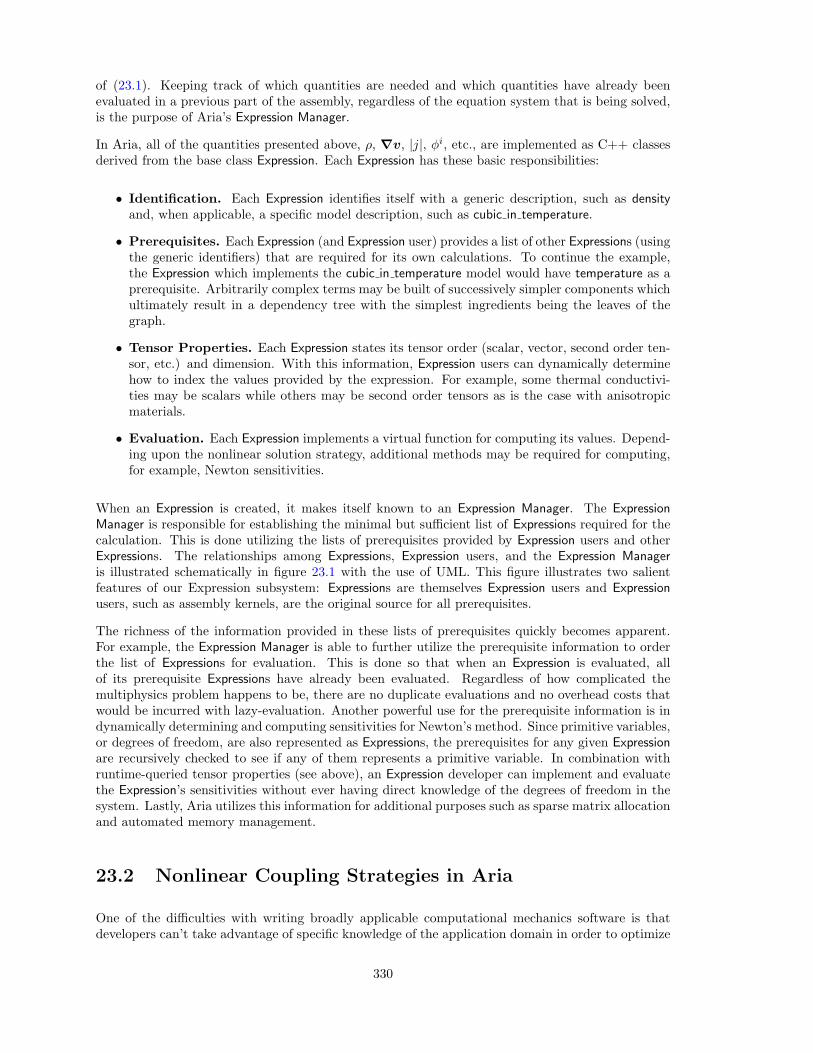
of (23.1). Keeping track of which quantities are needed and which quantities have already beenevaluated in a previous part of the assembly, regardless of the equation system that is being solved,is the purpose of Aria’s Expression Manager.
In Aria, all of the quantities presented above, ρ, ∇v, |j|, φi, etc., are implemented as C++ classesderived from the base class Expression. Each Expression has these basic responsibilities:
• Identification. Each Expression identifies itself with a generic description, such as densityand, when applicable, a specific model description, such as cubic in temperature.
• Prerequisites. Each Expression (and Expression user) provides a list of other Expressions (usingthe generic identifiers) that are required for its own calculations. To continue the example,the Expression which implements the cubic in temperature model would have temperature as aprerequisite. Arbitrarily complex terms may be built of successively simpler components whichultimately result in a dependency tree with the simplest ingredients being the leaves of thegraph.
• Tensor Properties. Each Expression states its tensor order (scalar, vector, second order ten-sor, etc.) and dimension. With this information, Expression users can dynamically determinehow to index the values provided by the expression. For example, some thermal conductivi-ties may be scalars while others may be second order tensors as is the case with anisotropicmaterials.
• Evaluation. Each Expression implements a virtual function for computing its values. Depend-ing upon the nonlinear solution strategy, additional methods may be required for computing,for example, Newton sensitivities.
When an Expression is created, it makes itself known to an Expression Manager. The ExpressionManager is responsible for establishing the minimal but sufficient list of Expressions required for thecalculation. This is done utilizing the lists of prerequisites provided by Expression users and otherExpressions. The relationships among Expressions, Expression users, and the Expression Manageris illustrated schematically in figure 23.1 with the use of UML. This figure illustrates two salientfeatures of our Expression subsystem: Expressions are themselves Expression users and Expressionusers, such as assembly kernels, are the original source for all prerequisites.
The richness of the information provided in these lists of prerequisites quickly becomes apparent.For example, the Expression Manager is able to further utilize the prerequisite information to orderthe list of Expressions for evaluation. This is done so that when an Expression is evaluated, allof its prerequisite Expressions have already been evaluated. Regardless of how complicated themultiphysics problem happens to be, there are no duplicate evaluations and no overhead costs thatwould be incurred with lazy-evaluation. Another powerful use for the prerequisite information is indynamically determining and computing sensitivities for Newton’s method. Since primitive variables,or degrees of freedom, are also represented as Expressions, the prerequisites for any given Expressionare recursively checked to see if any of them represents a primitive variable. In combination withruntime-queried tensor properties (see above), an Expression developer can implement and evaluatethe Expression’s sensitivities without ever having direct knowledge of the degrees of freedom in thesystem. Lastly, Aria utilizes this information for additional purposes such as sparse matrix allocationand automated memory management.
23.2 Nonlinear Coupling Strategies in Aria
One of the difficulties with writing broadly applicable computational mechanics software is thatdevelopers can’t take advantage of specific knowledge of the application domain in order to optimize
330
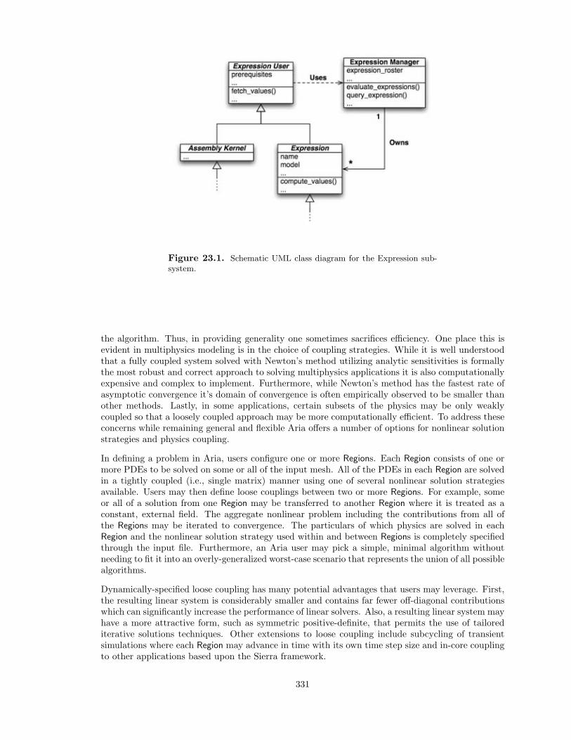
Figure 23.1. Schematic UML class diagram for the Expression sub-system.
the algorithm. Thus, in providing generality one sometimes sacrifices efficiency. One place this isevident in multiphysics modeling is in the choice of coupling strategies. While it is well understoodthat a fully coupled system solved with Newton’s method utilizing analytic sensitivities is formallythe most robust and correct approach to solving multiphysics applications it is also computationallyexpensive and complex to implement. Furthermore, while Newton’s method has the fastest rate ofasymptotic convergence it’s domain of convergence is often empirically observed to be smaller thanother methods. Lastly, in some applications, certain subsets of the physics may be only weaklycoupled so that a loosely coupled approach may be more computationally efficient. To address theseconcerns while remaining general and flexible Aria offers a number of options for nonlinear solutionstrategies and physics coupling.
In defining a problem in Aria, users configure one or more Regions. Each Region consists of one ormore PDEs to be solved on some or all of the input mesh. All of the PDEs in each Region are solvedin a tightly coupled (i.e., single matrix) manner using one of several nonlinear solution strategiesavailable. Users may then define loose couplings between two or more Regions. For example, someor all of a solution from one Region may be transferred to another Region where it is treated as aconstant, external field. The aggregate nonlinear problem including the contributions from all ofthe Regions may be iterated to convergence. The particulars of which physics are solved in eachRegion and the nonlinear solution strategy used within and between Regions is completely specifiedthrough the input file. Furthermore, an Aria user may pick a simple, minimal algorithm withoutneeding to fit it into an overly-generalized worst-case scenario that represents the union of all possiblealgorithms.
Dynamically-specified loose coupling has many potential advantages that users may leverage. First,the resulting linear system is considerably smaller and contains far fewer off-diagonal contributionswhich can significantly increase the performance of linear solvers. Also, a resulting linear system mayhave a more attractive form, such as symmetric positive-definite, that permits the use of tailorediterative solutions techniques. Other extensions to loose coupling include subcycling of transientsimulations where each Region may advance in time with its own time step size and in-core couplingto other applications based upon the Sierra framework.
331
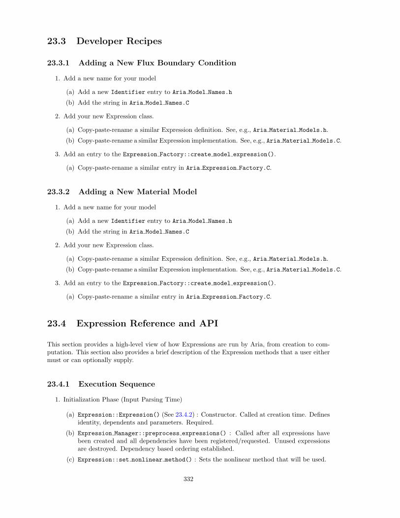
23.3 Developer Recipes
23.3.1 Adding a New Flux Boundary Condition
1. Add a new name for your model
(a) Add a new Identifier entry to Aria Model Names.h
(b) Add the string in Aria Model Names.C
2. Add your new Expression class.
(a) Copy-paste-rename a similar Expression definition. See, e.g., Aria Material Models.h.
(b) Copy-paste-rename a similar Expression implementation. See, e.g., Aria Material Models.C.
3. Add an entry to the Expression Factory::create model expression().
(a) Copy-paste-rename a similar entry in Aria Expression Factory.C.
23.3.2 Adding a New Material Model
1. Add a new name for your model
(a) Add a new Identifier entry to Aria Model Names.h
(b) Add the string in Aria Model Names.C
2. Add your new Expression class.
(a) Copy-paste-rename a similar Expression definition. See, e.g., Aria Material Models.h.
(b) Copy-paste-rename a similar Expression implementation. See, e.g., Aria Material Models.C.
3. Add an entry to the Expression Factory::create model expression().
(a) Copy-paste-rename a similar entry in Aria Expression Factory.C.
23.4 Expression Reference and API
This section provides a high-level view of how Expressions are run by Aria, from creation to com-putation. This section also provides a brief description of the Expression methods that a user eithermust or can optionally supply.
23.4.1 Execution Sequence
1. Initialization Phase (Input Parsing Time)
(a) Expression::Expression() (See 23.4.2) : Constructor. Called at creation time. Definesidentity, dependents and parameters. Required.
(b) Expression Manager::preprocess expressions() : Called after all expressions havebeen created and all dependencies have been registered/requested. Unused expressionsare destroyed. Dependency based ordering established.
(c) Expression::set nonlinear method() : Sets the nonlinear method that will be used.
332
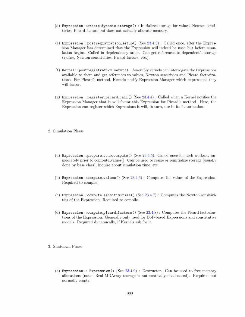
(d) Expression::create dynamic storage() : Initializes storage for values, Newton sensi-tivies, Picard factors but does not actually allocate memory.
(e) Expression::postregistration setup() (See 23.4.3) : Called once, after the Expres-sion Manager has determined that the Expression will indeed be used but before simu-lation begins. Called in depdendency order. Can get references to dependent’s storage(values, Newton sensitivities, Picard factors, etc.).
(f) Kernel::postregistration setup() : Assembly kernels can interrogate the Expressionsavailable to them and get references to values, Newton sensitivies and Picard factoriza-tions. For Picard’s method, Kernels notify Expression Manager which expressions theywill factor.
(g) Expression::register picard call() (See 23.4.4) : Called when a Kernel notifies theExpression Manager that it will factor this Expression for Picard’s method. Here, theExpression can register which Expressions it will, in turn, use in its factorization.
2. Simulation Phase
(a) Expression::prepare to recompute() (See 23.4.5): Called once for each workset, im-mediately prior to compute values(). Can be used to resize or reinitialize storage (usuallydone by base class), inquire about simulation time, etc.
(b) Expression::compute values() (See 23.4.6) : Computes the values of the Expression.Required to compile.
(c) Expression::compute sensitivities() (See 23.4.7) : Computes the Newton sensitivi-ties of the Expression. Required to compile.
(d) Expression::compute picard factors() (See 23.4.8) : Computes the Picard factoriza-tions of the Expression. Generally only used for DoF-based Expressions and constitutivemodels. Required dynamically, if Kernels ask for it.
3. Shutdown Phase
(a) Expression:: Expression() (See 23.4.9) : Destructor. Can be used to free memoryallocations (note: Real MDArray storage is automatically deallocated). Required butnormally empty.
333
23.4.2 Constructor
23.4.3 postregistration setup()
23.4.4 register picard prerequisites()
23.4.5 prepare to recompute()
23.4.6 compute values()
23.4.7 compute sensitivities()
23.4.8 compute picard factors()
23.4.9 Destructor
23.5 Newton Sensitivity Checking for Expressions
When you run Aria you can ask it to look for sensitivity errors in every Expression if you’re usingNewton’s method. If activated, Aria will compare the analytic sensitivities provided by each expres-sion with numerically computed values. This feature is enabled by adding the command line option-arialog sens check to Aria. If you’re using the sierra tool to run Aria, then add -O ‘‘-arialogsens check’’ (including quotes) to the sierra command line. The same holds if you’re runningthe Arpeggio application.
You can also run the entire test suite with Jacobian checking enabled by adding -u aria args =‘‘-arialog sens check’’ to the runtest command line.
23.6 Profiling
It’s a good idea to profile the code before spending time trying to optimizing and performancetuning. Fortunately, profiling is pretty easy to do. On Linux, one approach is to use the gproftool. To profile code with gprof, you’ll need to compile with the -pg option. The easiest way to dothis is to set environment variables USER CFLAGS and USER LDFLAGS to -pg. In the bash/ksh/zshshell, use, e.g., export USER CFLAGS=-pg and in tcsh/csh use setenv USER CFLAGS -pg. You’llonly get detailed profileing information for code compiled and linked with this flag so you may wantto recompile some of the framework too. You can profile debug or optimized code.
With the instrumented executable, run Aria as you normally would. This will generate a filecalled gmon.out. Lastly, run gprof to analyze the data: gprof executable > gprof.txt whereexecutable is the executable (probably including an absolute or relative path) used in the run.The output stored in gprof.txt will give you some real data telling where the real bottle necks are.
334
23.7 Purify: Memory Analysis and Debugging
1. Build Aria on Linux. This works for both optimized and debug modes but use debug if youwant to see line numbers in Purify.
2. Copy the complete link line into a file.
3. Add -show option to mpiCC.
4. Remove the -static option from the link line arguments.
5. Adjust any path to Apps aria.o if necessary.
6. Put which mpiCC on the previous line to verify you’re gettingmpiCC from /usr/local/mpi/sierra/mpich/1.2.5.2/gcc-3.2.2/bin/.
7. You might also verify gcc is version 3.2.2 (gcc -v).
8. Source the script.
9. Copy the link line (start with g++ ...) and paste it into a file.
10. Preface g++ with purify, e.g., purify -always-use-cache-dir -cache-dir=‘pwd‘/ g++...
11. Source this script and it will instrument your executable. It takes a while...
12. Optionally verify that the executable is purifyed by running ldd aria.x
13. Copy executable to aria/bin directory, removing the .tmp extension.
14. Run it standalone (via sierra, runtest or by hand) or with TotalView.
23.8 Building Against Other Projects
Sometimes it can be very usefull to build against changes that have been made in a different project.For example, if you are waiting for a project’s changes to be checked in but would like to startdeveloping against those changes in another project. To do this with the SNTools build tool youcan use the -a option to build. The argument to this option is the XML file for each product youwant to include in your build. So, if you want to use the version of Krino found in a project locatedin /path/to/project/ then you would add -a /path/to/project/krino/krino sn.xml to yournormal build command line.
23.9 Interfacing with MATLAB
23.9.1 Reading Aria Matrices Into MATLAB
This is sort of an “old” way of getting matrices into MATLAB but it still works just fine.
From Matt Hopkins:
You can read a .mtx matrix into MATLAB via the following. Let my matrix.mtx be the matrixsitting in the debug output path you’re interested in.
335
>> A_ascii = load(’my_matrix.mtx’);>> A = spconvert(A_ascii(2:end,:));
And now A is in MATLAB’s sparse matrix format. It even ignores the zeros in the .mtx file (doesnot allocate space for them).
From there you can do some pretty nifty things. spy(A) does sort of what matvis does (graphicalview of matrix nonzeros). condest(A) estimates the 1-norm condition number of A (might take awhile for large A). Etc.
23.9.2 Interfacing Aria from within MATLAB
Russell Hooper is developing a pretty sophisticated MATLAB interace that allows you to controlAria and probe nonlinear and linear solver data structures directly from within MATLAB. This israpidly evolving so no details are given here... except for how to build and run Aria/MATLAB.
This recipe is taken from an email exchange between Matt Hopkins and Russell Hooper in earlyApril 2006. It most likely only works on Linux.
% setenv LD_LIBRARY_PATH /usr/local/matlab/7.2/bin/glnx86:\$LD_LIBRARY_PATH
% build aria -j8 -a /home/rhoope/Trilinos_6.0 \CXXFLAGS="-I/usr/local/matlab/7.2/extern/include/" \-a /home/rhoope/projects/noxMatlabStable/equationsolver \LDFLAGS="-L/usr/local/matlab/7.2/bin/glnx86 -leng"
If you want to build a debug version, add “-g” to both the CXXFLAGS and LDFLAGS.
To execute aria, first invoke sierra aria -i input.i --script-only. Then copy the file sierra.shinto another, ie opt.sh. Finally, remove the “-o logfilename” argument from opt.sh so that yourrun is truly interactive.
23.10 Error Handling
Traditional techniques for error handling of numerous and varried. Sometimes functions will returnspecial values indicating success or failure of the call. Sometimes global variables or flags are set toindicate an error has occurred. Sometimes abort() is simply called (bad!).
C++ and the SIERRA Framework offer facilities to support error handling. The two primaryerror handling techniques are exception handling and assertions. Both of these can be combined toimplement Design by Contract though this is not formally done in Aria.
Whether one should use an exception or an assertion is sometimes a subtle question. In general,assertions should be used for cases where the error is not likely to occur due merely to user input.However, assertions can also be useful for computationally expensive tests which would adverselyaffect production calculations.
336
23.10.1 Exception Handling
C++ offers exception handling and the SIERRA Framework utility library provides a parallel-safelayer for exception handling. Because exceptions in C++ are ordinary classes, applications maychoose to specialize exceptions for handling and detecting specific failure modes. When SIERRAexceptions are used in conjuction with the SIERRA diagnostic tracing facility, it is possibly to geta stacktrace (or sometimes a partial one) that illustrates the code path the where the exeption wasthrown.
In most cases, Aria developers do not need to worry about catching exceptions (they’re noramllyfatal errors). The top-level SIERRA Framework routine run sierra() handles the responsibilityof catching any uncaught exceptions, converting them into parallel exceptions if necessary, andpropogating the exception to any other processors.
If the reader is not already familiar with exception handling in C++, a good place to start is withStroustrup (2000). In it’s simplest form, SIERRA exceptions can be used as follows.
#include <util/Exception.h>// ...if(something_bad_happened)sierra::Exception x("Nice descriptive error message.");throw x;
The sierra::Exception class inherrits from std::string and so it supports all of std::string’soperations, most notably the + (concatentaion) operator.
#include <util/Exception.h>// ...if(something_bad_happened)sierra::Exception x("Nice descriptive error message.");x += " More info here.";throw x;
Additionally, the sierra::Exception class supports the put-to operator, <<, for stream-like han-dling.
#include <util/Exception.h>// ...if(something_bad_happened)sierra::Exception x;x << "Nice descriptive error message."<< " More info here.";
throw x;
However, in order to keep the sierra::Exception class light weight, it does not inherrit fromstd::ostringstream. Instead, operator<< is only defined for the most common objects, such asstrings, integers, floats/doubles, etc. The consequence of this is that if you define a class with
337
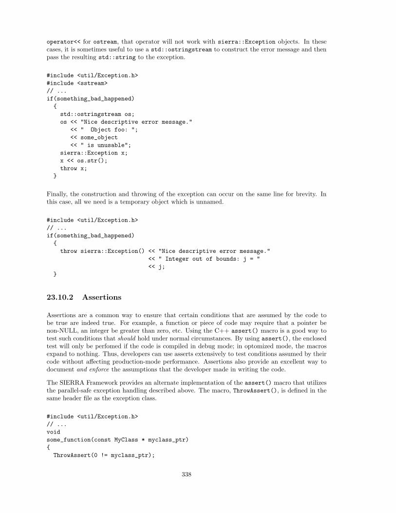
operator<< for ostream, that operator will not work with sierra::Exception objects. In thesecases, it is sometimes useful to use a std::ostringstream to construct the error message and thenpass the resulting std::string to the exception.
#include <util/Exception.h>#include <sstream>// ...if(something_bad_happened)std::ostringstream os;os << "Nice descriptive error message."
<< " Object foo: ";<< some_object<< " is unusable";
sierra::Exception x;x << os.str();throw x;
Finally, the construction and throwing of the exception can occur on the same line for brevity. Inthis case, all we need is a temporary object which is unnamed.
#include <util/Exception.h>// ...if(something_bad_happened)throw sierra::Exception() << "Nice descriptive error message."
<< " Integer out of bounds: j = "<< j;
23.10.2 Assertions
Assertions are a common way to ensure that certain conditions that are assumed by the code tobe true are indeed true. For example, a function or piece of code may require that a pointer benon-NULL, an integer be greater than zero, etc. Using the C++ assert() macro is a good way totest such conditions that should hold under normal circumstances. By using assert(), the enclosedtest will only be perfomed if the code is compiled in debug mode; in optomized mode, the macrosexpand to nothing. Thus, developers can use asserts extensively to test conditions assumed by theircode without affecting production-mode performance. Assertions also provide an excellent way todocument and enforce the assumptions that the developer made in writing the code.
The SIERRA Framework provides an alternate implementation of the assert() macro that utilizesthe parallel-safe exception handling described above. The macro, ThrowAssert(), is defined in thesame header file as the exception class.
#include <util/Exception.h>// ...voidsome_function(const MyClass * myclass_ptr)ThrowAssert(0 != myclass_ptr);
338
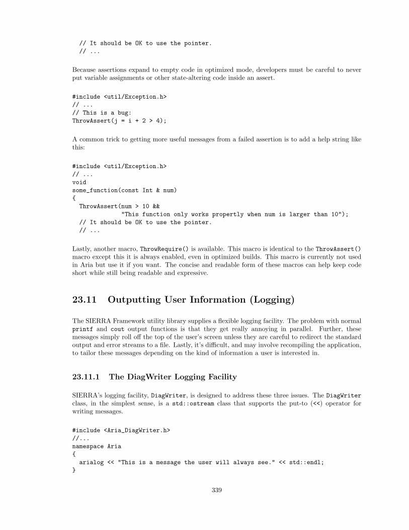
// It should be OK to use the pointer.// ...
Because assertions expand to empty code in optimized mode, developers must be careful to neverput variable assignments or other state-altering code inside an assert.
#include <util/Exception.h>// ...// This is a bug:ThrowAssert(j = i + 2 > 4);
A common trick to getting more useful messages from a failed assertion is to add a help string likethis:
#include <util/Exception.h>// ...voidsome_function(const Int & num)ThrowAssert(num > 10 &&
"This function only works propertly when num is larger than 10");// It should be OK to use the pointer.// ...
Lastly, another macro, ThrowRequire() is available. This macro is identical to the ThrowAssert()macro except this it is always enabled, even in optimized builds. This macro is currently not usedin Aria but use it if you want. The concise and readable form of these macros can help keep codeshort while still being readable and expressive.
23.11 Outputting User Information (Logging)
The SIERRA Framework utility library supplies a flexible logging facility. The problem with normalprintf and cout output functions is that they get really annoying in parallel. Further, thesemessages simply roll off the top of the user’s screen unless they are careful to redirect the standardoutput and error streams to a file. Lastly, it’s difficult, and may involve recompiling the application,to tailor these messages depending on the kind of information a user is interested in.
23.11.1 The DiagWriter Logging Facility
SIERRA’s logging facility, DiagWriter, is designed to address these three issues. The DiagWriterclass, in the simplest sense, is a std::ostream class that supports the put-to (<<) operator forwriting messages.
#include <Aria_DiagWriter.h>//...namespace Ariaarialog << "This is a message the user will always see." << std::endl;
339
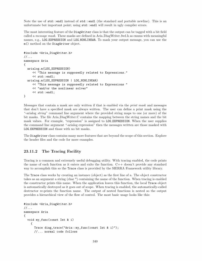
Note the use of std::endl instead of std::endl (the standard and portable newline). This is anunfortunate but important point; using std::endl will result in ugly compiler errors.
The most interesting feature of the DiagWriter class is that the output can be tagged with a bit fieldcalled a message mask. These masks are defined in Aria DiagWriter fwd.h as enums with meaningfulnames, e.g., LOG EXPRESSION and LOG NONLINEAR. To mask your output message, you can use them() method on the DiagWriter object.
#include <Aria_DiagWriter.h>//...namespace Ariaarialog.m(LOG_EXPRESSION)
<< "This message is supposedly related to Expressions."<< std::endl;
arialog.m(LOG_EXPRESSION | LOG_NONLINEAR)<< "This message is supposedly related to Expressions "<< "and/or the nonlinear solver"<< std::endl;
Messages that contain a mask are only written if that is enabled via the print mask and messagesthat don’t have a specified mask are always written. The user can define a print mask using the“-arialog string” command line argument where the provided string maps to one (or more) of thebit masks. The file Aria DiagWriter.C contains the mapping between the string names and the bitmask values. For example, “expression” is assigned to LOG EXPRESSION. When the user suppliesthe command line argument “-arialog expression” then the messages written are those masked withLOG EXPRESSION and those with no bit masks.
The DiagWriter class contains many more features that are beyond the scope of this section. Explorethe header files and the code for more examples.
23.11.2 The Tracing Facility
Tracing is a common and extremely useful debugging utility. With tracing enabled, the code printsthe name of each function as it enters and exits the function. C++ doesn’t provide any standardway to accomplish this so the Trace class is provided by the SIERRA Framework utility library.
The Trace class works by creating an instance (object) as the first line of a. The object constructortakes as an argument a string (char *) containing the name of the function. When tracing is enabledthe constructor prints this name. When the application leaves this function, the local Trace objectis automatically destroyed as it goes out of scope. When tracing is enabled, the automatically-calleddestructor re-prints the function name. The output of nested functions is nested so the outputprovides a hierarchical view of the flow of control. The most basic usage looks like this:
#include <Aria_DiagWriter.h>//...namespace Ariavoid my_func(const Int & i)Trace diag_trace("Aria::my_func(const Int & i)");//... normal code follows
340
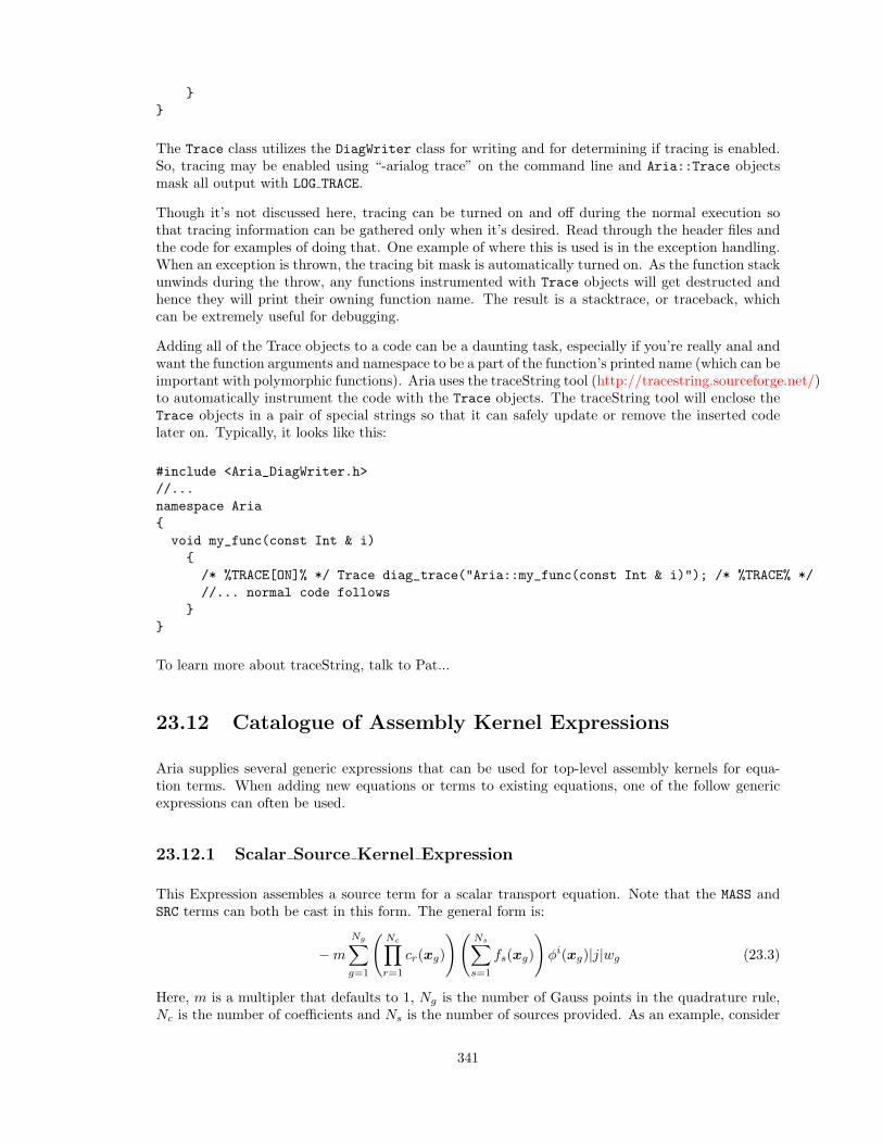
The Trace class utilizes the DiagWriter class for writing and for determining if tracing is enabled.So, tracing may be enabled using “-arialog trace” on the command line and Aria::Trace objectsmask all output with LOG TRACE.
Though it’s not discussed here, tracing can be turned on and off during the normal execution sothat tracing information can be gathered only when it’s desired. Read through the header files andthe code for examples of doing that. One example of where this is used is in the exception handling.When an exception is thrown, the tracing bit mask is automatically turned on. As the function stackunwinds during the throw, any functions instrumented with Trace objects will get destructed andhence they will print their owning function name. The result is a stacktrace, or traceback, whichcan be extremely useful for debugging.
Adding all of the Trace objects to a code can be a daunting task, especially if you’re really anal andwant the function arguments and namespace to be a part of the function’s printed name (which can beimportant with polymorphic functions). Aria uses the traceString tool (http://tracestring.sourceforge.net/)to automatically instrument the code with the Trace objects. The traceString tool will enclose theTrace objects in a pair of special strings so that it can safely update or remove the inserted codelater on. Typically, it looks like this:
#include <Aria_DiagWriter.h>//...namespace Ariavoid my_func(const Int & i)/* %TRACE[ON]% */ Trace diag_trace("Aria::my_func(const Int & i)"); /* %TRACE% *///... normal code follows
To learn more about traceString, talk to Pat...
23.12 Catalogue of Assembly Kernel Expressions
Aria supplies several generic expressions that can be used for top-level assembly kernels for equa-tion terms. When adding new equations or terms to existing equations, one of the follow genericexpressions can often be used.
23.12.1 Scalar Source Kernel Expression
This Expression assembles a source term for a scalar transport equation. Note that the MASS andSRC terms can both be cast in this form. The general form is:
−m
Ng∑g=1
(Nc∏r=1
cr(xg)
)(Ns∑s=1
fs(xg)
)φi(xg)|j|wg (23.3)
Here, m is a multipler that defaults to 1, Ng is the number of Gauss points in the quadrature rule,Nc is the number of coefficients and Ns is the number of sources provided. As an example, consider
341
the term, ∫Ωe
ρCp∂T
∂t|j|φi dΩe =
Ng∑g=1
ρCp∂T
∂t|j|φiwg (23.4)
In this example, Nr = 2 with c1 = ρ and c2 = Cp; Ns = 1 with f1 = ∂T∂t ; and m = −1. As a side
note, in the code the quantities |j| and wg are treated as additional coefficients for convenience.
23.12.2 Scalar Advection Kernel Expression
This Expression assembles an advection term for a scalar transport equation. The general form is:
m
Ng∑g=1
(Nc∏r=1
cr(xg)
)va · ∇S(xg)φi(xg)|j|wg (23.5)
Here, m is a multipler that defaults to 1, Ng is the number of Gauss points in the quadrature rule,Nc is the number of coefficients, va is a configurable advection velocity and S is a scalar field. Asan example, consider the term,
∫Ωe
ρCpv · ∇T |j|φi dΩe =Ng∑g=1
ρCpv · ∇T |j|φiwg (23.6)
In this example, Nr = 2 with c1 = ρ and c2 = Cp; S = T ; va = v; and m = 1. As a side note, inthe code the quantities |j| and wg are treated as additional coefficients for convenience.
23.12.3 Scalar Diffusion Kernel Expression
This Expression assembles a diffusion term for a scalar transport equation. The general form is:
m
Ng∑g=1
(Nc∏r=1
cr(xg)
)(NF∑k=1
F k(xg)
)· ∇φi(xg)|j|wg (23.7)
Here, m is a multipler that defaults to 1, Ng is the number of Gauss points in the quadrature rule,Nc is the number of coefficients and NF is the number of flux models provided. As an example,consider the term, ∫
Ωe
q∇φi|j|dΩe =Ng∑g=1
q · ∇φi|j|wg (23.8)
In this example, Nr = 0; NF = 1 with F1 = q where q is the Fourier heat flux, q = −κ∇T ; andm = 1. As a side note, in the code the quantities |j| and wg are treated as additional coefficientsfor convenience.
23.12.4 Vector Source Kernel Expression
This Expression assembles a source term for a vector transport equation. Note that the MASS andSRC terms can both be cast in this form. The general form is:
−m
Ng∑g=1
(Nc∏r=1
cr(xg)
)(Ns∑s=1
fs(xg)
)φi(xg)|j|wg (23.9)
342
Here, m is a multipler that defaults to 1, Ng is the number of Gauss points in the quadrature rule,Nc is the number of coefficients and Nk is the number of sources provided. In this case, the sourcesfs are vector quantities. As an example, consider the term,∫
Ωe
ρ∂v
∂t|j|φi dΩe =
Ng∑g=1
ρ∂v
∂t|j|φiwg (23.10)
In this example, N1 = 2 with c1 = ρ, Ns = 1 with f1 = ∂v∂t ; and m = −1. As a side note, in the
code the quantities |j| and wg are treated as additional coefficients for convenience.
23.12.5 Vector Advection Kernel Expression
This Expression assembles an advection term for a vector transport equation. The general form is:
m
Ng∑g=1
(Nc∏r=1
cr(xg)
)va · ∇V (xg)φi(xg)|j|wg (23.11)
Here, m is a multipler that defaults to 1, Ng is the number of Gauss points in the quadrature rule,Nc is the number of coefficients, va is a configurable advection velocity and V is a vector field. Asan example, consider the term,∫
Ωe
ρv · ∇v|j|φi dΩe =Ng∑g=1
ρv · ∇v|j|φiwg (23.12)
In this example, Nr = 1 with c1 = ρ; V = v; va = v; and m = 1. As a side note, in the code thequantities |j| and wg are treated as additional coefficients for convenience.
23.12.6 Vector Diffusion Kernel Expression
This Expression assembles a diffusion term for a vector transport equation. The general form is:
m
Ng∑g=1
(Nc∏r=1
cr(xg)
)(NF∑k=1
F tk(xg)
): ∇
(ejφ
i(xg))|j|wg (23.13)
Here, m is a multipler that defaults to 1, Ng is the number of Gauss points in the quadrature rule,Nc is the number of coefficients and NF is the number of flux models provided. As an example,consider the term, ∫
Ωe
T t : ∇(ejφ
i)|j|dΩe =
Ng∑g=1
T t : ∇(ejφ
i)|j|wg (23.14)
In this example, Nr = 0; NF = 1 with F1 = T where T is the Newtonian stress, T = µ (∇v + ∇vt)−pI; and m = 1. As a side note, in the code the quantities |j| and wg are treated as additionalcoefficients for convenience.
23.13 Errors and Warnings How-To
Editorial note: This How-To is mostly taken from Dave Bauer’s collection of How-Tos. Minorchanges include formatting, editorial corrections and possibly additioinal information related to Aria.
343
23.13.1 Reporting
There are several types of warnings and exceptions that occur in sierra. Warnings are informationalmessages to the user which may effect the results, but which will allow the execution to complete.Dooms are error conditions which will allow the program to continue to a point, but will not allowit to complete. Often these are within the parser when you want the parser to continue to plod onahead but not actually execute the code. Exceptions occur when all bets are off.
The Warning and Doom classes send their assembled message to the sierra reporter at destruction.The Exception classes send their assembled message to the sierra reporter within the catch block.
The warning and exception classes will all accept the put-to operator (<<) with plain old data. Sinceit is easy to put useful information to the user/developer in the message, please do so. For warningsdirected to developers, it is recommended that the message be terminated with a
<< std::endl << WarnTrace;
For exceptions, always use
<< std::endl << StackTrace;
WarnTrace and StackTrace generate a ”pretty” source file and line number message. If the messageis purely informational for the user the std::endl and WarnTrace for the message should be omitted.
These are the include files:
#include <util/Exception.h>// throw sierra#exception declarations#include <util/ExceptionReport.h>// sierra reporter and#RuntimeWarning declarations
The RuntimeUserError class should be thrown in place of RuntimeError when it was the user’s faultthat the program died. This generally means that the input deck has an error that a RuntimeDoomed,the preferred method since it allows the parser, etc to continue, cannot handle since a seg fault orthe like is imminent. It kills the output of the traceback since the user really does care and will onlycause confusion.
Also, don’t put the WarnTrace or StackTrace to the RuntimeUserError.
The following code snippets serve as examples for the warning, doomed and exception conditions.
class_tag *Parser::prsr_handler_x(const Prsr_CommandValues & value)
if (runtime_warning_condition)sierra::RuntimeWarning() << "My useful message about " <<some_data << std::endl << WarnTrace;
if (runtime_exception_condition)throw sierra::RuntimeError() << "My useful message about " <<
344
some_data << std::endl << StackTrace;
if (runtime_exception_condition)throw sierra::RuntimeUserError() << "My useful message about "<< some_data;
if (parse_handler_warning_condition)sierra::RunWarning() << "My useful message about " <<some_data << std::endl << WarnTrace;
if (parse_handler_doomed_condition)sierra::RuntimeDoomed() << "My useful message about " <<some_data << std::endl << WarnTrace;
23.13.2 Throttling a Specific Warning or Doom
If a particular warnings is going to be repeated countless times, you can request a unique messageid from sierra using
int message_id = sierra::get_next_message_id();int message_id = sierra::get_next_message_id(int max_messages_displayed);
and pass message id to the message constructor. This value is often stored within the function thatgenerates the message using a static variable. This technique may not be suitable for all situations.Only a limited number of messages of each id are sent to the sierra reporter.
if (runtime_warning_condition) static message_id = get_next_message_id();
sierra::RuntimeWarning(message_id) << "My useful message about" << some_data << std::endl << WarnTrace;
if (parse_handler_warning_condition) static message_id = get_next_message_id();sierra::Prsr::ParseWarning(value, message_id) << "My usefulmessage about " << some_data << std::endl << WarnTrace;
if (parse_handler_doomed_condition) static message_id = get_next_message_id();sierra::Prsr::ParseDoomed(value, message_id) << "My usefulmessage about " << some_data << std::endl << WarnTrace;
345
if (parse_handler_exception_condition) static message_id = get_next_message_id();sierra::Prsr::ParseError(value, message_id) << "My usefulmessage about " << some_data << std::endl << WarnTrace;
23.13.3 Setting Output Throttles
There are several functions which can throttle the amount of data which is displayed.
To set the maximum number of warnings or dooms before an exception is thrown:
void sierra::set_max_warnings(int max_warnings);void sierra::set_max_dooms(int max_dooms);
int sierra::get_max_warnings();int sierra::get_max_dooms();
To set the maximum number of warnings displayed. Each occurance is still counted, but not dis-played. Dooms are always displayed.
void sierra::set_max_displayed_warnings(int max_display_warnings);int sierra::get_max_displayed_warnings();
To set the default maximum id messages to display, set get next message id() below:
int sierra::set_default_max_id_dispaly(intdefault_max_id_displayed)int sierra::set_default_max_id_dispaly(intdefault_max_id_displayed)
23.13.4 Sierra Exception Reporter
What is this sierra reporter thing you ask? It goes like this: When a Warning or a Doom classis destroyed, report exception() is called with the message. report exception() then calls theregistered report exception handler. The report exception handler has a signature of
(*)(const char *message, int type)
and is set with set report exception handler(). Sierra sets this to use the sierra report exception handler()which writes the message to sierra::Env::output().
If you want special decorations around your messages during executeion, you can change the reporter.The parse, instantiation and commit handlers are set by run sierra().
23.13.5 The Output versus OutputP0 Dilema
Unfortunately, determining what to do with the output from multiple processors can be an issue.If a warning is going to happen on all processors, you may want to wrapper it with a test for
346
processor zero and only output it there. The default report exception handler sends the outputto Env::output()
23.13.6 Getting Counts
To get the number of warnings issued, even if not displayed:
get_warning_count()
To get the number of dooms issued, even if not displayed:
get_doomed_count()
23.13.7 Traceback and Tracing
The traceback messages are generated by the Trace and Traceback classes upon there destruction.So, if the source code has had trace objects constructed, the stack trace will show them. If efficiencybecomes an issue, the #define app TRACE ENABLED can be undefined which will cause the Traceand Traceback classes to be empty.
The trace object can be used to extract function signature information. The getFunctionSpec(),getFunctionName(), getFunctionShortName(), getFunctionClass(), getFunctionShortClass()and getFunctionNamespace() functions will all extract appropriate information from the functionsignature.
The program /usr/netpub/traceString/traceString (on Linux) can be used to quickly place thetrace objects in your source code. I suggest editing the results and placing [ON], [TRACEBACK] or[NONE] after the first %TRACE as in %TRACE[NONE]%. These will instruct traceString which objecttype to create. Then, rerun traceString. I set it to NONE for functions which will execute manymany times or cannot throw an error or not have much value in a stack trace (accessors, etc). I setit to TRACEBACK if it will not be useful to see traced during a trace run, but be useful in a traceback.And ON otherwise which incurs some overhead that enables the conditional runtime trace.
Here is the .traceString file I use and suggest be used throughout sierra.
[START_OF_ROUTINE_PATTERNS]default : Trace trace__("$(FQNAME)");off :Off :OFF :none :None :NONE :spec : static Tracespec trace__("$(FQNAME)");Spec : static Tracespec trace__("$(FQNAME)");SPEC : static Tracespec trace__("$(FQNAME)");on : Trace trace__("$(FQNAME)");On : Trace trace__("$(FQNAME)");ON : Trace trace__("$(FQNAME)");traceback : Traceback trace__("$(FQNAME)");Traceback : Traceback trace__("$(FQNAME)");TRACEBACK : Traceback trace__("$(FQNAME)");
347
23.13.8 Deriving from a Sierra Exception
When deriving a new exception from the framework exceptions and using the put-to (<<) operator,you must include the following template functions in your class or
throw MyError() << "My error message cause of " << x;
will certainly fail. It only took me a day to relearn this, but:
If MyError does not implement a put-to operator, it uses the base classes put to operator, sayRuntimeError. Well, the RuntimeError put-to operator returns a reference to a RuntimeError, sonow you are going to be throwing a RuntimeError exception not a MyError exception. This is onlyan issue when using the temporaries. By putting the MyError() construction on the same line asthe throw. I.e.,
MyError x;x << "My error message cause of " << x;throw x;
works fine since we are actually throwing x, a MyError object.
So, add these if you derive from a sierra exception and wish to throw the temporary object and usethe put operator all in one pretty line:
class MyError : public RuntimeError
.
.
.inline MyError& operator<<(ExceptionString& (*f)(ExceptionString
&)) f(*this);return *this;
template <class T>inline MyError &operator<<(const T &t) RuntimeError::operator<<(t);return *this;
;
23.13.9 path name()
When generating error messages with object names, use the path name() form rather than justname. This generates a dot (.) separated list of names from the Procedure on down.
23.13.10 abort() – Don’t use it
abort() does not provide any useful information when the application dies. By replacing abort callswith Warnings, Dooms and Exceptions, the code will be easier to maintain and the user will get
348
better diagnostic output.
23.13.11 Apub Parser Base – Useful for parsing, not needed for error re-porting
This class stashes useful information from within a parser that is likely to be needed after parsing.The runtime error reporting routines handle error reporting making the line number and commandvalue information redundant for error reporting.
23.14 Diagnostic Writer How-To
Editorial note: This How-To is mostly taken from Dave Bauer’s collection of How-Tos. Minorchanges include formatting, editorial corrections and possibly additioinal information related to Aria.
This document briefly describes the implementation of the diagnostic writer and masked basedoutput. The diagnostic writer is intended to replace debug level output with but masked baseddiagnostic output. By utilizing the diagnostic writer, your normal output can be separated orinterleaved with the diagnostic output, the diagnostic output can the enabled/disabled at specifictimes during a run, and entire classes can be output by simply putting the object to the diagnosticwriter.
23.14.1 Output
Application output falls into three classes. Normal execution output, warning and error out-put, and diagnostic output. Normal execution output is handled via the Env::outputP0() andEnv::output() functions and by the application diagnostic writer. Warning and error output ishandled by the RuntimeWarning, RuntimeDoomed and runtime exception classes (RuntimeError,LogicError, etc), which is eventually written to the env output stream and the diagnostic outptustream. And diagnostic output is for selected operationally descriptive output.
In many cases, the diagnostic output is utilized as the primary output stream when selectable levelof user output is desired. With thay in mind, an InfoWriter class has been written. However,additional discussion is required to complete the design and implementation of this class for primaryapplication output.
23.14.2 Diagnostic Writer
The diagnostic writer allows you to write diagnostic information to the diagnostics stream by spec-ifying the content from the command line or the input deck. It a debug level built on a bit mask.
Since there are many applications and libraries, there are several diagnostic writers. Each diagnosticwriter has its own bit mask, command line parser and writer. However, they all share a commondiagnostic stream. So, output from each diagnostic writer is properly interleaved.
Each application defines it own diagnostic writer. This is generally defined within the app DiagWriter fwd.h,app DiagWriter.h, app DiagWriter.C files. The app DiagWriter fwd.h file defines the LOG xxx bitassignments. These values are used to specify the type of message to be written. The app DiagWriter.hrarely needs to be modified. It declares the daignostic writer for the application or library. Theapp DiagWriter.C files defines the parser which provides names for the LOG xxx bit masks.
349
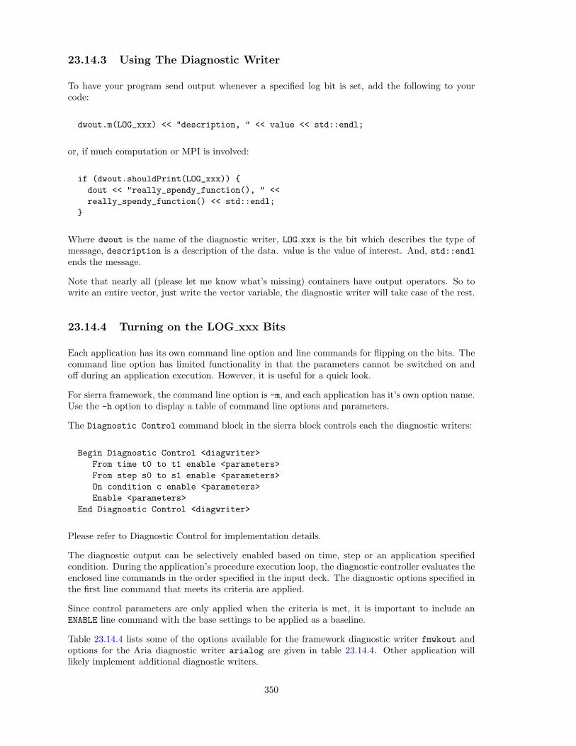
23.14.3 Using The Diagnostic Writer
To have your program send output whenever a specified log bit is set, add the following to yourcode:
dwout.m(LOG_xxx) << "description, " << value << std::endl;
or, if much computation or MPI is involved:
if (dwout.shouldPrint(LOG_xxx)) dout << "really_spendy_function(), " <<really_spendy_function() << std::endl;
Where dwout is the name of the diagnostic writer, LOG xxx is the bit which describes the type ofmessage, description is a description of the data. value is the value of interest. And, std::endlends the message.
Note that nearly all (please let me know what’s missing) containers have output operators. So towrite an entire vector, just write the vector variable, the diagnostic writer will take case of the rest.
23.14.4 Turning on the LOG xxx Bits
Each application has its own command line option and line commands for flipping on the bits. Thecommand line option has limited functionality in that the parameters cannot be switched on andoff during an application execution. However, it is useful for a quick look.
For sierra framework, the command line option is -m, and each application has it’s own option name.Use the -h option to display a table of command line options and parameters.
The Diagnostic Control command block in the sierra block controls each the diagnostic writers:
Begin Diagnostic Control <diagwriter>From time t0 to t1 enable <parameters>From step s0 to s1 enable <parameters>On condition c enable <parameters>Enable <parameters>
End Diagnostic Control <diagwriter>
Please refer to Diagnostic Control for implementation details.
The diagnostic output can be selectively enabled based on time, step or an application specifiedcondition. During the application’s procedure execution loop, the diagnostic controller evaluates theenclosed line commands in the order specified in the input deck. The diagnostic options specified inthe first line command that meets its criteria are applied.
Since control parameters are only applied when the criteria is met, it is important to include anENABLE line command with the base settings to be applied as a baseline.
Table 23.14.4 lists some of the options available for the framework diagnostic writer fmwkout andoptions for the Aria diagnostic writer arialog are given in table 23.14.4. Other application willlikely implement additional diagnostic writers.
350
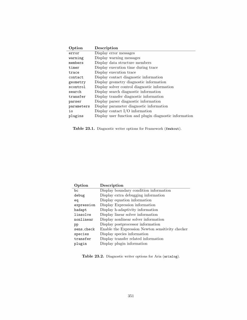
Option Descriptionerror Display error messageswarning Display warning messagesmembers Display data structure memberstimer Display execution time during tracetrace Display execution tracecontact Display contact diagnostic informationgeometry Display geometry diagnostic informationscontrol Display solver control diagnostic informationsearch Display search diagnostic informationtransfer Display transfer diagnostic informationparser Display parser diagnostic informationparameters Display parameter diagnostic informationio Display contact I/O informationplugins Display user function and plugin diagnostic information
Table 23.1. Diagnostic writer options for Framework (fmwkout).
Option Descriptionbc Display boundary condition informationdebug Display extra debugging informationeq Display equation informationexpression Display Expression informationhadapt Display h-adaptivity informationlinsolve Display linear solver informationnonlinear Display nonlinear solver informationpp Display postprocessor informationsens check Enable the Expression Newton sensitivity checkerspecies Display species informationtransfer Display transfer related informationplugin Display plugin information
Table 23.2. Diagnostic writer options for Aria (arialog).
351
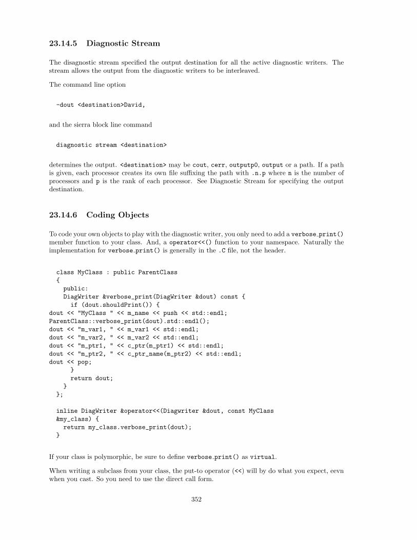
23.14.5 Diagnostic Stream
The disagnostic stream specified the output destination for all the active diagnostic writers. Thestream allows the output from the diagnostic writers to be interleaved.
The command line option
-dout <destination>David,
and the sierra block line command
diagnostic stream <destination>
determines the output. <destination> may be cout, cerr, outputp0, output or a path. If a pathis given, each processor creates its own file suffixing the path with .n.p where n is the number ofprocessors and p is the rank of each processor. See Diagnostic Stream for specifying the outputdestination.
23.14.6 Coding Objects
To code your own objects to play with the diagnostic writer, you only need to add a verbose print()member function to your class. And, a operator<<() function to your namespace. Naturally theimplementation for verbose print() is generally in the .C file, not the header.
class MyClass : public ParentClasspublic:DiagWriter &verbose_print(DiagWriter &dout) const if (dout.shouldPrint())
dout << "MyClass " << m_name << push << std::endl;ParentClass::verbose_print(dout).std::endl();dout << "m_var1, " << m_var1 << std::endl;dout << "m_var2, " << m_var2 << std::endl;dout << "m_ptr1, " << c_ptr(m_ptr1) << std::endl;dout << "m_ptr2, " << c_ptr_name(m_ptr2) << std::endl;dout << pop;
return dout;
;
inline DiagWriter &operator<<(Diagwriter &dout, const MyClass&my_class) return my_class.verbose_print(dout);
If your class is polymorphic, be sure to define verbose print() as virtual.
When writing a subclass from your class, the put-to operator (<<) will by do what you expect, eevnwhen you cast. So you need to use the direct call form.
352
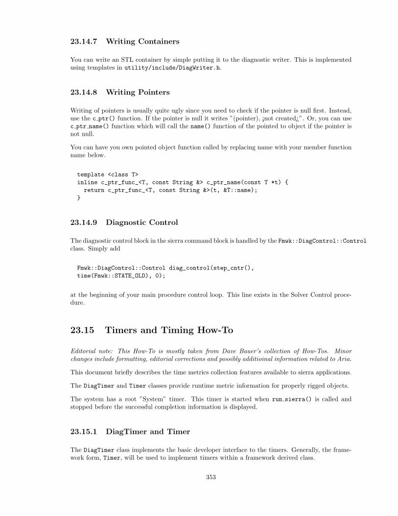
23.14.7 Writing Containers
You can write an STL container by simple putting it to the diagnostic writer. This is implementedusing templates in utility/include/DiagWriter.h.
23.14.8 Writing Pointers
Writing of pointers is usually quite ugly since you need to check if the pointer is null first. Instead,use the c ptr() function. If the pointer is null it writes ”(pointer), ¡not created¿”. Or, you can usec ptr name() function which will call the name() function of the pointed to object if the pointer isnot null.
You can have you own pointed object function called by replacing name with your member functionname below.
template <class T>inline c_ptr_func_<T, const String &> c_ptr_name(const T *t) return c_ptr_func_<T, const String &>(t, &T::name);
23.14.9 Diagnostic Control
The diagnostic control block in the sierra command block is handled by the Fmwk::DiagControl::Controlclass. Simply add
Fmwk::DiagControl::Control diag_control(step_cntr(),time(Fmwk::STATE_OLD), 0);
at the beginning of your main procedure control loop. This line exists in the Solver Control proce-dure.
23.15 Timers and Timing How-To
Editorial note: This How-To is mostly taken from Dave Bauer’s collection of How-Tos. Minorchanges include formatting, editorial corrections and possibly additioinal information related to Aria.
This document briefly describes the time metrics collection features available to sierra applications.
The DiagTimer and Timer classes provide runtime metric information for properly rigged objects.
The system has a root ”System” timer. This timer is started when run sierra() is called andstopped before the successful completion information is displayed.
23.15.1 DiagTimer and Timer
The DiagTimer class implements the basic developer interface to the timers. Generally, the frame-work form, Timer, will be used to implement timers within a framework derived class.
353
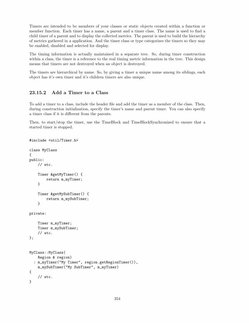
Timers are intended to be members of your classes or static objects created within a function ormember function. Each timer has a name, a parent and a timer class. The name is used to find achild timer of a parent and to display the collected metrics. The parent is used to build the hierarchyof metrics gathered in a application. And the timer class or type categorizes the timers so they maybe enabled, disabled and selected for display.
The timing information is actually maintained in a separate tree. So, during timer constructionwithin a class, the timer is a reference to the real timing metric information in the tree. This designmeans that timers are not destroyed when an object is destroyed.
The timers are hierarchical by name. So, by giving a timer a unique name among its siblings, eachobject has it’s own timer and it’s children timers are also unique.
23.15.2 Add a Timer to a Class
To add a timer to a class, include the header file and add the timer as a member of the class. Then,during construction initialization, specify the timer’s name and parent timer. You can also specifya timer class if it is different from the parents.
Then, to start/stop the timer, use the TimeBlock and TimeBlockSynchronized to ensure that astarted timer is stopped.
#include <util/Timer.h>
class MyClasspublic:
// etc.
Timer &getMyTimer() return m_myTimer;
Timer &getMySubTimer() return m_mySubTimer;
private:
Timer m_myTimer;Timer m_mySubTimer;// etc.
;
MyClass::MyClass(Region & region)
: m_myTimer("My Timer", region.getRegionTimer()),m_mySubTimer("My SubTimer", m_myTimer)
// etc.
354
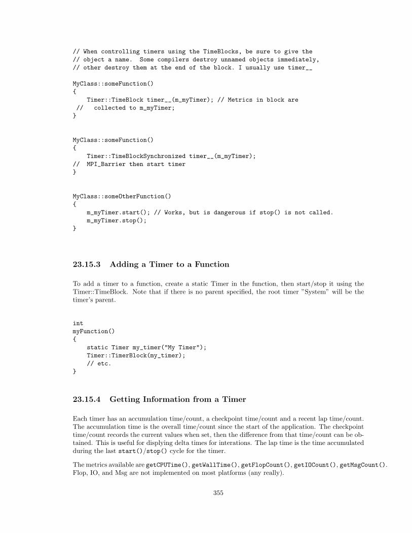
// When controlling timers using the TimeBlocks, be sure to give the// object a name. Some compilers destroy unnamed objects immediately,// other destroy them at the end of the block. I usually use timer__
MyClass::someFunction()
Timer::TimeBlock timer__(m_myTimer); // Metrics in block are// collected to m_myTimer;
MyClass::someFunction()
Timer::TimeBlockSynchronized timer__(m_myTimer);// MPI_Barrier then start timer
MyClass::someOtherFunction()
m_myTimer.start(); // Works, but is dangerous if stop() is not called.m_myTimer.stop();
23.15.3 Adding a Timer to a Function
To add a timer to a function, create a static Timer in the function, then start/stop it using theTimer::TimeBlock. Note that if there is no parent specified, the root timer ”System” will be thetimer’s parent.
intmyFunction()
static Timer my_timer("My Timer");Timer::TimerBlock(my_timer);// etc.
23.15.4 Getting Information from a Timer
Each timer has an accumulation time/count, a checkpoint time/count and a recent lap time/count.The accumulation time is the overall time/count since the start of the application. The checkpointtime/count records the current values when set, then the difference from that time/count can be ob-tained. This is useful for displying delta times for interations. The lap time is the time accumulatedduring the last start()/stop() cycle for the timer.
The metrics available are getCPUTime(), getWallTime(), getFlopCount(), getIOCount(), getMsgCount().Flop, IO, and Msg are not implemented on most platforms (any really).
355
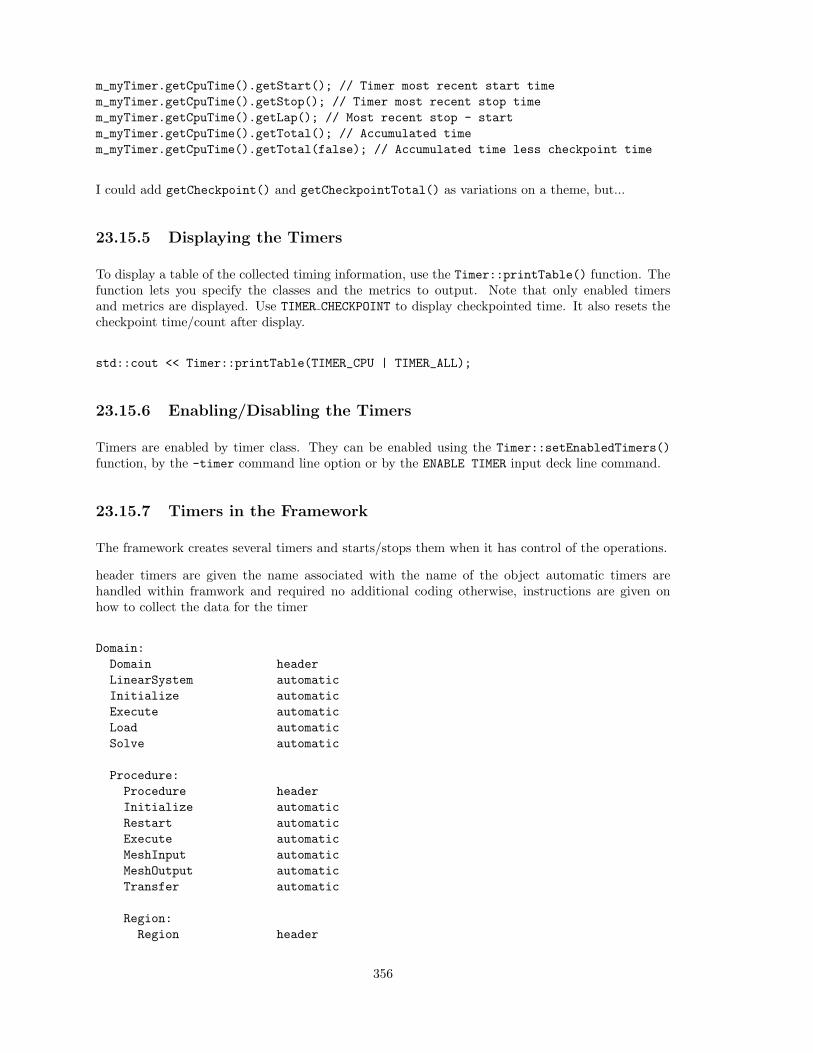
m_myTimer.getCpuTime().getStart(); // Timer most recent start timem_myTimer.getCpuTime().getStop(); // Timer most recent stop timem_myTimer.getCpuTime().getLap(); // Most recent stop - startm_myTimer.getCpuTime().getTotal(); // Accumulated timem_myTimer.getCpuTime().getTotal(false); // Accumulated time less checkpoint time
I could add getCheckpoint() and getCheckpointTotal() as variations on a theme, but...
23.15.5 Displaying the Timers
To display a table of the collected timing information, use the Timer::printTable() function. Thefunction lets you specify the classes and the metrics to output. Note that only enabled timersand metrics are displayed. Use TIMER CHECKPOINT to display checkpointed time. It also resets thecheckpoint time/count after display.
std::cout << Timer::printTable(TIMER_CPU | TIMER_ALL);
23.15.6 Enabling/Disabling the Timers
Timers are enabled by timer class. They can be enabled using the Timer::setEnabledTimers()function, by the -timer command line option or by the ENABLE TIMER input deck line command.
23.15.7 Timers in the Framework
The framework creates several timers and starts/stops them when it has control of the operations.
header timers are given the name associated with the name of the object automatic timers arehandled within framwork and required no additional coding otherwise, instructions are given onhow to collect the data for the timer
Domain:Domain headerLinearSystem automaticInitialize automaticExecute automaticLoad automaticSolve automatic
Procedure:Procedure headerInitialize automaticRestart automaticExecute automaticMeshInput automaticMeshOutput automaticTransfer automatic
Region:Region header
356
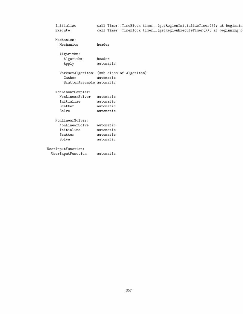
Initialize call Timer::TimeBlock timer__(getRegionInitializeTimer()); at beginning of initialize()Execute call Timer::TimeBlock timer__(getRegionExecuteTimer()); at beginning of execute()
Mechanics:Mechanics header
Algorithm:Algorithm headerApply automatic
WorksetAlgorithm: (sub class of Algorithm)Gather automaticScatterAssemble automatic
NonLinearCoupler:NonLinearSolver automaticInitialize automaticScatter automaticSolve automatic
NonLinearSolver:NonLinearSolve automaticInitialize automaticScatter automaticSolve automatic
UserInputFunction:UserInputFunction automatic
357

358
Glossary
coefficient: Each field that is represented by a basis function expansion has a set of coefficients thatare used in that expansion. For example, the three dimensional velocity vector represented byan eight node, tri-linear hex element has eight coefficients. In this example, each coefficient isalso a vector with three components.
This is consistent with the Sierra data model wherein vectors and tensors are single-entity datatypes.
Although for certain basis function representations the coefficients may be the exact value ofthe field at a point this is not the case in general.
component: The number of values required to describe a field at a point. Equal to the tensor di-mension raised to the power of the tensor order. For example, temperature has one component,velocity has 3 components (in 3 dimensions) and stress has 9 components.
dof: An entry in the vector of uknowns, i.e. , in the linear solver solution vector.
field: The physical variable of interest, e.g. , temperature or velocity.
multidof: A field is a multidof if it contains more than one component
359

360
References
Ted Belytschko, Wing Kam Liu, and Brian Moran. Nonlinear Finite Elements for Continua andStructures. John Wiley and Sons, 2004. 3.11, 1, 2, 10.21.3, 10.29.3
T. D. Blake and J. De Coninck. The influence of solid-liquid interactions on dynamic wetting. Adv.Colloid and Interface Sci., 96:21–36, 2002. 6.14.19
Pavel B. Bochev, Clark R. Rohrmann, and Max D. Gunzburger. Stabilization of low-order mixedfinite elements for the Stokes equations. SIAM J. Numer. Anal., 44(1):82–101, 2006. 4.14
Erik Boman, Karen Devine, Robert Heaphy, Bruce Hendrickson, William Mitchell, MatthewSt. John, and Courtenay Vaughan. Zoltan home page. http://www.cs.sandia.gov/Zoltan,1999. 18
Javier Bonet and Richard D. Wood. Nonlinear Continuum Mechanics for Finite Element Analysis.Cambridge University Press, 1997. 3.11, 1, 10.21.3, 10.29.3
R. A. Cairncross, P. R. Schunk, T. A. Baer, R. R. Rao, and P. A. Sackinger. A finite element methodfor free surface flows of incompressible fluids in three dimensions. part i. boundary fitted meshmotion. Int. J. Numer. Methd. Fluids, 33:375–403, 2000. 6.14.11
Ken S. Chen, Gregory H. Evens, Richard S. Larson, David R. Noble, and William G. Houf. Finalreport on LDRD project: A phenomenological model for multicomponent transport with simul-taneous electrochemical reactions in concentrated solutions. SAND 2000-0207, Sandia NationalLaboratories, Albuquerque, NM 87185, USA, January 2000. 8.2.8
W. M. Deen. Analysis of Transport Phenomena. Topics in Chemical Engineering. Oxford UniversityPress, New York, 1998. 3.1
Karen Devine, Bruce Hendrickson, Erik Boman, Matthew St. John, and Courtenay Vaughan. Zoltan:A Dynamic Load Balancing Library for Parallel Applications; User’s Guide. Sandia NationalLaboratories, Albuquerque, NM, 1999. Tech. Report SAND99-1377 http://www.cs.sandia.gov/Zoltan/ug html/ug.html. 18
Karen Devine, Erik Boman, Robert Heaphy, Bruce Hendrickson, and Courtenay Vaughan. Zoltandata management services for parallel dynamic applications. Computing in Science and Engineer-ing, 4(2):90–97, 2002. 18
Clark R. Dohrmann and Pavel B. Bochev. A stabilized finite element method for the Stokes problembased on polynomial pressure projections. Int. J. Num. Meth. Fluids, 46:183–201, 2004. 4.14
D. K. Gartling. NACHOS II - a finite element computer program for incompressible flow prob-lems. part I - theoretical background. Technical Report SAND86-1816, Sandia National Labs,Albuquerque, NM, USA, April 1986. 12.5
T. Hughes, L. P. Franca, and M. Balestra. A new finite element formulation for computational fluiddynamics: V. circumventing the babuska-brezzi condition: a stable petrov-galerkin formulationof the stokes problem accomodating equal-order interpolations. Comput. Methods Appl. Mech.Engrg., 59:85–99, 1986. 4.14
I. M. Krieger. Rheology of monodisperse latices. Adv. Colloid Interface Sci., 3:111–136, 1972. 10.40.8
361
Lawrence E. Malvern. Introduction to the Mechanics of a Continuous Medium. Series in Engineeringof the Physical Sciences. Prentice-Hall, Upper Saddle River, NJ, USA, 1969. 3.11, 1, 3
George E. Mase. Theory and Problems of Continuum Mechanics. Schaum’s Outline Series. McGraw-Hill, New York, NY, USA, 1970. 3.11, 1, 3, 4, 6, 7
P. K. Notz, S. R. Subia, M. H. Hopkins, and P. A. Sackinger. A novel approach to solving highlycoupled equations in a dynamic, extensible and efficient way. In M. Papadrakakis, E. Onate, andB. Schrefler, editors, Computation Methods for Coupled Problems in Science and Engineering,page 129, Barcelona, Spain, April 2005. Intl. Center for Num. Meth. in Engng. (CIMNE). 23.1
Patrick K. Notz. SourceForge project page for Aria. https://sourceforge.sandia.gov/projects/aria/, a. 1.1
Patrick K. Notz. Aria home page. http://aria.sandia.gov/, b. 1.1
Bjarne Stroustrup. The C++ Programming Language, Special Edition. Addison Wesley, Reading,MA, 2000. 23.10.1
The SNTools Project. SNTools SourceForge Project. Online. 2.1, 2.2
362
Index
AABSOLUTE TOLERANCE, 217, 219ACCEPT SOLUTION AFTER MAXIMUM NONLIN-
EAR ITERATIONS, 183ACTIVE FOR PROCEDURE, 318, 320ACTIVE PERIODS, 283, 284ADAPT MESH ON, 233ADAPTIVE STRATEGY, 234, 235adaptivity, 233ADAPTIVITY CONTROLLER, 234ADD SURFACE, 283, 286ADDITIONAL STEPS, 291, 293, 296, 300, 302, 303, 307,
308, 312, 316ADDITIONAL TIMES, 291, 293, 296, 300, 302, 303, 307,
308, 312, 316ADVANCE, 149–151, 153, 155–157, 159, 161–165, 167,
169, 171Algorithm Debug Level, 242, 244ALL FIELDS, 143, 146assert, 338AT STEP, 291, 294, 296, 301, 303, 304, 307, 309, 312, 317AT TIME, 291, 294, 296, 301, 302, 304, 307, 309, 312, 317AZTEC EQUATION SOLVER, 261
BBC CIRC X, 57BC CIRC Y, 57BC CONST, 58BC DISTING, 73BC ENFORCEMENT, 251, 257, 261, 267BC FLUX, 63
CAPILLARY, 68CONSTANT, 63CONSTANT TRACTION, 68ELECTRIC TRACTION, 69ENCLOSURE RADIATION, 63FLOW HYDROSTATIC, 69LASER, 63LASER WELD, 64LATENT HEAT, 66NAT CONV, 67, 68OPEN FLOW, 70PRESSURE, 70RAD, 67SLIP, 71SPOT WELD, 65TRANSIENT TRACTION, 71VAPOR COOLING, 67WETTING SPEED BLAKE LS, 72
BC LINEAR, 58BC LINEAR IN TIME, 58BC PARAB, 59BC PERIODIC LINEAR IN TIME, 59BC PERIODIC STEP IN TIME, 60BC ROTATING X, 60BC ROTATING Y, 61BC TRANSLATE, 61BC UNIDIRECTIONAL FLOW X, 61BC UNIDIRECTIONAL FLOW Y, 62BEAM FLANGE THICKNESS, 319, 327BEAM HEIGHT, 319, 326
BEAM REFERECNE AXIS, 319, 327BEAM SECTION, 319, 326BEAM WALL THICKNESS, 319, 327BEAM WIDTH, 319, 326BETA, 89
CONSTANT, 89CONVERTED, 90LINEAR, 90
BLOCKING SURFACES, 283, 286BSP TREE MAX DEPTH, 277, 278BULK VISCOSITY, 90
CONSTANT, 90CURING FOAM, 91
CCauchy stress, 37Check Geometry, 242, 245COLOR GRAPH USING DISTANCE1, 194, 207, 220,
221COLORING ALGORITHM, 194, 207COLORING REORDERING, 194, 207COMPONENT SEPARATOR CHARACTER, 296, 299,
312, 315COMPUTE AT OUTPUT, 236, 237COMPUTE METRIC, 236COMPUTE OVERKILL SOLUTION USING REFINE
LEVEL, 236, 238COMPUTE RULE, 277, 278COMPUTE STEP INTERVAL, 236, 237CONSTRAIN, 87CONVERGED WHEN, 173, 174CONVERGENCE TOLERANCE, 282COPY, 143, 144COUPLING, 281, 282COURANT LIMIT, 175, 176CTE, 91
CONSTANT, 92curing epoxy foam
bulk viscosity, 91density, 94energy source, 78, 79species source, 85specific heat, 79, 125thermal conductivity, 130viscosity, 137
CURRENT DENSITY, 92BASIC, 93OHMS LAW, 93
CYCLE COUNT, 291, 293
DDAMPER AREA, 319, 323Darcy’s law, 104, 106, 110, 117, 118DATABASE NAME, 284, 289, 291, 296, 307, 310, 312DATABASE TYPE, 291, 292, 296, 297, 307, 311–313DEACTIVATE, 318, 320Debug Memory, 242, 250DEBUG OUTPUT LEVEL, 251, 256, 261, 266DEBUG OUTPUT PATH, 251, 256, 261, 266Debug Processor Number, 242, 249debugging, 335
363

Deformation gradient, 36DENSITY, 93
CONSTANT, 93CURING FOAM, 94EXP DECAY, 94IDEAL GAS, 94INCOMPRESSIBLE IDEAL GAS, 95POLYNOMIAL, 95THERMAL, 96USER FUNCTION, 96
DEPOSIT SPECIFIC INTERNAL ENERGY, 319, 322Deterministic Decomposition, 242, 243DEVIATORIC PARAMETER, 319, 323DiagWriter, 339DISTINGUISH MATRIX FREE FILLS, 194, 205distinguishing conditions, 73
KINEMATIC, 74PLUGIN, 74POLYNOMIAL, 74WETTING SPEED BLAKE LS, 75
DUMP INITIAL GUESS VECTOR, 194, 208DUMP JACOBIAN MATRIX, 194, 208DUMP LINEAR SOLUTION VECTOR, 194, 208DUMP RESIDUAL VECTOR, 194, 208
EEDGE VARIABLES, 296, 299, 312, 315EFFECTIVE MODULI MODEL, 319, 328ELASTICITY FORMULATION, 49ELECTRIC DISPLACEMENT, 99
BASIC, 100LINEAR, 100
ELECTRICAL CONDUCTIVITY, 97CONSTANT, 98EXPONENTIAL, 98FROM RESISTANCE, 98POLYNOMIAL, 98TBC, 99THERMAL, 99
ELECTRICAL PERMITTIVITY, 100CONSTANT, 100
ELECTRICAL RESISTANCE, 101CONSTANT, 101EXPONENTIAL, 101FROM CONDUCTIVITY, 102POLYNOMIAL, 102USER FUNCTION, 102
ELEMENT COORDINATE SYSTEM, 319, 325ELEMENT INITIAL STRAINXX, 319, 324ELEMENT INITIAL STRAINXY, 319, 324ELEMENT INITIAL STRAINXZ, 319, 324ELEMENT INITIAL STRAINYY, 319, 324ELEMENT INITIAL STRAINYZ, 319, 325ELEMENT INITIAL STRAINZZ, 319, 324ELEMENT NUMERICAL FORMULATION, 319, 322ELEMENT VARIABLES, 296, 298, 312, 314EMISSIVITY, 103, 283, 285
CONSTANT, 103EMISSIVITY FUNCTION, 283, 285EMISSIVITY SUBROUTINE, 283, 285ENABLE REBALANCE, 241ENCLOSURE DEFINITION, 283ENTHALPHY, 104
CONSTANT, 104EQ CONTINUITY, 43EQ CURRENT, 44EQ ENERGY, 44EQ LEVEL SET, 45
EQ MESH, 45EQ MOMENTUM, 46EQ SHEAR, 46EQ SOLID, 47EQ SPECIES, 47EQ Stress Tensor Projection, 49EQ SUSPENSON, 48EQ VOLTAGE, 48Equation
Continuity, 29Current, 34Energy, 30Fluid Momentum, 32Mass Conservation, 29Solid Momentum, 33Species, 31Stress Tensor Projection, 35Suspension, 34Voltage, 33
EQUATION OF STATE, 104IDEAL GAS, 104
error estimation, 233ERROR ESTIMATION CONTROLLER, 236ERROR ESTIMATOR, 236, 237ESTIMATE ERROR FOR, 233EVENT, 147–151, 153, 155–157, 159–165, 167, 169, 171,
172exception handling, 337EXCLUDE GHOSTED, 143, 146EXCLUDE MATERIALS, 239, 240Expression
compute picard factors(), 334compute sensitivities(), 334compute values(), 334postregistration setup(), 334prepare to recompute(), 334register picard prerequisites(), 334Constructor, 334Destructor, 334
FFACE VARIABLES, 296, 299, 312, 315FEI ERROR BEHAVIOR, 252, 259, 262, 269FEI OUTPUT LEVEL, 251, 256, 261, 266FILTER NONLINEAR SOLUTION, 183FINITE DIFFERENCE METHOD, 194, 204, 220FIX EMPTY ROWS, 220, 222FLOOR VALUE, 217, 219FORCING TERM INITIAL TOLERANCE, 193, 200, 222,
225FORCING TERM MAXIMUM TOLERANCE, 193, 200,
222, 225FORCING TERM METHOD, 193, 199, 222, 225FORCING TERM MINIMUM TOLERANCE, 193, 200,
222, 225FROM, 143, 145
GGEOMETRIC TOLERANCE, 277, 278GLOBAL ERROR TOLERANCE, 234, 236GLOBAL VARIABLES, 296, 297, 312, 313Green strain, 36Green-Lagrange strain, 36
Hh-adaptivity, 233HEARTBEAT, 302HEAT CONDUCTION, 105
364
BASIC, 105CONVECTED ENTHALPY, 105FOURIERS LAW, 105
HEAT OF VAPORIZATION, 106CONSTANT, 106
HEMICUBE MAX SUBDIVIDES, 277, 279HEMICUBE MIN SEPARATION, 277, 279HEMICUBE RESOLUTION, 277, 278HISTORY OUTPUT, 307HOURGLASS, 319, 321
IIC CIRC X, 53IC CIRC Y, 53IC CONSTANT, 54IC COUETTE SH, 55IC COUETTE X, 54IC COUETTE Y, 54IC LINEAR, 55IC PARAB, 56IC READ FILE, 55ILL CONDITIONING THRESHOLD, 194, 202ILU FILL, 251, 255, 261, 265ILU GRAPH FILL, 194, 203ILU OMEGA, 261, 265ILU OVERLAP, 194, 202ILU THRESHOLD, 251, 255, 261, 265ILUT DROP TOLERANCE, 194, 203ILUT FILL FACTOR, 194, 203Imbalance Tolerance, 242, 244INACTIVE FOR PROCEDURE, 318, 320INACTIVE PERIODS, 283, 284INCLUDE MATERIALS, 239, 240INITIAL DELTAT, 172, 173INITIAL TIME STEP SIZE, 175, 178INITIALIZE, 146, 171INPUT DATABASE NAME, 284, 289, 291, 292INTEGRATED FLUX OUTPUT, 283, 286INTEGRATED POWER OUTPUT, 283, 286INTEGRATION RULE, 51interfacial tension, see SURFACE TENSIONINTERNAL ENERGY, 107
GAS PHASE, 107INTERPOLATE, 143, 144INTERPOLATION FUNCTION, 143, 145INTRINSIC PERMEABILITY, 106
CONSTANT, 107INVOLVE, 149–156, 158–164, 166–169, 171, 172
KKeep Cuts, 242, 245
LLABELS, 303, 306Lagrangian strain, 36Lame coefficients, 37LAMBDA, 108
CONSTANT, 108CONVERTED, 109
LEGEND, 303, 306LEVEL SET HEAVISIDE, 109
SMOOTH, 109LEVEL SET WIDTH, 109
CONSTANT, 110LINEAR BULK VISCOSITY, 319, 321LINEAR SOLVER OUTPUT FREQUENCY, 194, 207,
222, 227LINEAR STAGNATION TEST STEPS, 194, 206
LINEAR STAGNATION TEST TOLERANCE, 194, 206LINEAR SYSTEM TYPE, 222, 223load balancing, 241Load Balancing Method, 242, 243LOCA CONTINUATION SOLVER, 229Lock RCB Directions, 242, 245LOFTING FACTOR, 319, 323logging, 339
MMASS FLUX, 110
DARCY, 110MATERIAL, 318, 320MATLAB, interfacing, 335MATRIX FORMAT, 251, 258, 262, 268MATRIX FREE FINITE DIFFERENCE METHOD, 194,
204MATRIX FREE NONLINEAR, 149, 156, 158, 159, 164,
166, 167, 169, 171MATRIX FREE PERTURBATION COEFFICIENT LAMBDA,
194, 205, 220, 221MATRIX FREE PERTURBATION COEFFICIENT VALUE,
194, 205, 220, 221MATRIX REDUCTION, 251, 258, 262, 268MATRIX SCALING, 251, 257, 262, 267MATRIX VIEWER, 251, 259, 262, 269MAX AGE OF JACOBIAN, 193, 199, 222, 224MAX ELEMENTS, 234, 235MAX INNER ADAPT STEPS, 234, 235MAX OUTER ADAPT STEPS, 234MAX REPORTED VALUES, 218, 219MAXIMUM ITERATIONS, 193, 201, 222, 226, 251, 254,
261, 264, 282, 283MAXIMUM NONLINEAR ITERATIONS, 182, 193, 202MAXIMUM TIME STEP SIZE, 175, 176MEMBRANE SCALE THICKNESS, 319, 321memory analysis, 335MESH MOTION, 50mesh refinement, 233MESH STRESS, 110
ISOTHERMAL, 111LINEAR ELASTIC, 111NEOHOOKEAN ELASTIC, 112NONLINEAR ELASTIC, 112RESIDUAL, 113THERMAL, 113
MINIMUM NONLINEAR ITERATIONS, 183, 194, 206MINIMUM TIME STEP SIZE, 175, 178MOLECULAR WEIGHT, 113
CONSTANT, 114MOMENTUM STRESS, 114
FORMAL NEWTONIAN, 115INCOMPRESSIBLE NEWTONIAN, 114LS CAPILLARY, 114NEWTONIAN DILATIONAL, 115NEWTONIAN PRESSURE, 116NEWTONIAN VISCOUS, 116
MONITOR, 303, 306
NNODAL VARIABLES, 296, 298, 312, 314NODE VARIABLES, 296, 297, 312, 313NODES OUTSIDE REGION, 143, 145NODESET VARIABLES, 296, 299, 312, 315NONBLOCKING SURFACES, 283, 286NONLINEAR, 149, 151, 152, 159–162NONLINEAR ABSOLUTE RESIDUAL NORM TOLER-
ANCE, 193, 202
365
NONLINEAR ABSOLUTE UPDATE NORM TOLER-ANCE, 194, 206
NONLINEAR CORRECTION TOLERANCE, 181NONLINEAR DIRECTION METHOD, 193, 197NONLINEAR JACOBIAN OPERATOR, 193, 198NONLINEAR LINESEARCH METHOD, 193, 198, 228NONLINEAR ML COARSENING METHOD, 194, 210NONLINEAR ML COARSENING RATIO OBJECTIVE,
195, 211NONLINEAR ML DIMENSION NULLSPACE, 195, 213NONLINEAR ML FINITE DIFFERENCE ALPHA, 195,
215NONLINEAR ML FINITE DIFFERENCE BETA, 195,
215NONLINEAR ML FINITE DIFFERENCE CENTERED,
195, 215NONLINEAR ML FINITE DIFFERENCE FINE LEVEL,
195, 211NONLINEAR ML IS LINEAR PRECONDITIONER, 194,
210NONLINEAR ML IS MATRIXFREE, 195, 210NONLINEAR ML LINEAR SMOOTHER COARSEST,
195, 213NONLINEAR ML LINEAR SMOOTHER FINE, 195, 213NONLINEAR ML LINEAR SMOOTHER MED, 195, 213NONLINEAR ML LINEAR SMOOTHER SWEEPS COARS-
EST, 195, 214NONLINEAR ML LINEAR SMOOTHER SWEEPS FINE,
195, 213NONLINEAR ML LINEAR SMOOTHER SWEEPS MED,
195, 213NONLINEAR ML MAX COARSE SIZE, 195, 211NONLINEAR ML MAX NLEVEL, 195, 211NONLINEAR ML MAX NUMBER CYCLES, 195, 215NONLINEAR ML NONLINEAR SWEEPS COARSEST,
195, 214NONLINEAR ML NONLINEAR SWEEPS POST FINE,
195, 215NONLINEAR ML NONLINEAR SWEEPS POST MED,
195, 214NONLINEAR ML NONLINEAR SWEEPS PRE FINE,
195, 214NONLINEAR ML NONLINEAR SWEEPS PRE MED,
195, 214NONLINEAR ML NUM ITERATIONS LINCG COARS-
EST, 195, 212NONLINEAR ML NUM ITERATIONS LINCG FINE,
195, 212NONLINEAR ML NUM ITERATIONS LINCG MED,
195, 212NONLINEAR ML NUMBER PDES PER NODE, 195,
212NONLINEAR ML PRINT LEVEL, 195, 215NONLINEAR ML PROBLEM DIMENSION, 195, 212NONLINEAR ML RECALCULATION OFFSET, 195, 216NONLINEAR ML USE BROYDEN UPDATE, 195, 212NONLINEAR ML USE NLNCG LEVEL COARSEST,
195, 211NONLINEAR ML USE NLNCG LEVEL FINE, 195, 211NONLINEAR ML USE NLNCG LEVEL MED, 195, 211NONLINEAR PRECONDITIONING COMPUTE FRE-
QUENCY, 193, 199, 222, 224NONLINEAR RELATIVE RESIDUAL NORM TOLER-
ANCE, 194, 202NONLINEAR RELAXATION FACTOR, 182NONLINEAR RESIDUAL RATIO TOLERANCE, 182NONLINEAR RESIDUAL TOLERANCE, 181NONLINEAR SOLUTION STRATEGY, 181
NONLINEAR SOLVER METHOD, 193, 197NOX AZTECOO LINEAR SYSTEM, 195, 222NOX DEBUG BASE OPERATOR, 217, 218NOX DEBUG TEST OPERATOR, 217, 219NOX DEBUGGER BLOCK, 195, 217NOX EPETRA OPERATOR, 195, 220NOX LINESEARCH BLOCK, 196, 227NOX NONLINEAR EQUATION SOLVER, 193NOX NONLINEAR PRECONDITIONING METHOD, 193,
198NOX OUTPUT LEVEL, 194, 209NOX OUTPUT VALUE, 194, 209NUM LEVELS, 251, 258, 262, 268NUMBER OF INNER STEPS, 239NUMBER OF OUTER STEPS, 239NUMBER OF ROTATIONS, 277, 281NUMBER OF STEPS, 172, 174
OOctree Dimension, 242, 247Octree Max Objects, 242, 248Octree Method, 242, 247Octree Min Objects, 242, 248OPERATOR TYPE, 220, 221optimization, 334ORTHOG METHOD, 261, 266OUTPUT, 147, 149–156, 159–162, 164, 167, 168OUTPUT DATABASE NAME, 284, 289, 291, 292OUTPUT MESH, 296, 298, 312, 314OUTPUT NONLINEAR OBJECTS, 194, 209OUTPUT ON SIGNAL, 291, 295, 296, 301, 303, 304, 307,
309, 312, 317OUTPUT RULE, 277, 281–283Over Allocate Memory, 242, 244OVERLAY COUNT, 291, 292OVERWRITE, 291, 293, 296, 302, 307, 310, 312, 318
PPAIRWISE MONTE CARLO SAMPLE RULE, 277, 280PAIRWISE MONTE CARLO TOL1, 277, 280PAIRWISE MONTE CARLO TOL2, 277, 280PAIRWISE NUMBER OF MONTE CARLO SAMPLES,
277, 280PAIRWISE NUMBER OF VISIBILITY SAMPLES, 277,
279PAIRWISE VISIBILITY SAMPLE RULE, 277, 279PARAM-BOOL, 216, 217, 230, 231, 251, 252, 260, 261PARAM-INT, 216–218, 230, 231, 251, 252, 260–262PARAM-REAL, 216–218, 230, 251, 252, 260–262PARAM-STRING, 216–218, 230, 251, 252, 260–262PARAM-SUBLIST, 216, 217, 230, 231, 260, 261PARAMETERS FOR, 146, 172PARAMETERS FOR ARIA REGION, 173, 175PARAMETERS FOR BLOCK, 318PARTIAL ENCLOSURE AREA, 283, 286PARTIAL ENCLOSURE EMISSIVITY, 284, 287PARTIAL ENCLOSURE EMISSIVITY SUBROUTINE,
284, 288PARTIAL ENCLOSURE EMISSIVITY TEMPERATURE
FUNCTION, 284, 288PARTIAL ENCLOSURE EMISSIVITY TIME FUNCTION,
284, 287PARTIAL ENCLOSURE TEMPERATURE, 283, 287PARTIAL ENCLOSURE TEMPERATURE SUBROUTINE,
284, 287PARTIAL ENCLOSURE TEMPERATURE TIME FUNC-
TION, 284, 287performance tuning, 334
366
permeabilityintrinsic, 106relative, 118
PERTURBATION COEFFICIENT ALPHA, 194, 204, 220PERTURBATION COEFFICIENT BETA, 194, 204, 220,
221PHASE, 318, 320Piola-Kirchhoff stress, 37POINT AX, 319, 325POINT AY, 319, 325POINT AZ, 319, 325POINT BX, 319, 325POINT BY, 319, 326POINT BZ, 319, 326POINT SOURCE FOR . . . , 77Poisson’s ratio, 37POISSONS RATIO, 116
CONSTANT, 117POLYNOMIAL ORDER, 193, 201, 251, 255, 261, 264POROSITY, 117
CONSTANT, 118POLYNOMIAL, 118
porous flow, 104, 106, 107, 110, 117–120, 132POSTPROCESS, 271
CURRENT, 272DENSITY, 273ELECTRIC FIELD, 272FLUID FORCE, 272FLUID TRACTION, 271PRESSURE, 273PROJECTED FLUID STRESS XX, 275SPECIFIC HEAT, 274TEMPERATURE, 273THERMAL CONDUCTIVITY, 274VISCOSITY, 274
PRECISION, 303, 306PRECONDITION USING JACOBIAN, 222, 224PRECONDITIONER SUBDOMAIN OVERLAP, 251, 259,
262, 269PRECONDITIONING METHOD, 193, 196, 222, 224, 251,
253, 261, 263PRECONDITIONING PACKAGE, 194, 203, 222, 226PRECONDITIONING STEPS, 193, 201, 251, 255, 261,
264PREDICTOR FIELDS, 179PREDICTOR-CORRECTOR TOLERANCE, 175, 176,
179PRESSURE STABILIZATION, 50profiling, 334PSPG, 50PSPP, 50Purify, 335
QQUADRATIC BULK VISCOSITY, 319, 322QUANTITY OF INTEREST, 236, 238
RRADIOSITY DATABASE NAME, 284, 290RADIOSITY SOLVER, 281rcb max aspect ratio, 242, 250rcb recompute box, 242, 250rebalance, 241REBALANCE LOAD MEASURE, 241Rectilinear RCB Blocks, 242, 246REFINE INPUT MESH USING REFINE LEVEL, 239,
240refinement, 233
REGISTER REGION, 156, 158, 164, 166, 169, 170REGISTER TRANSFER, 156, 158, 164, 166, 169, 170RELATIVE PERMEABILITY, 118
CONSTANT, 119POLYNOMIAL, 119
RELATIVE TOLERANCE, 218, 219Renumber Partitions, 242, 247RESCUE BAD NEWTON SOLVE, 194, 205, 222, 227RESET COUNTER EACH TIME STEP, 193, 199RESIDUAL NORM SCALING, 251, 255, 261, 265RESIDUAL NORM TOLERANCE, 193, 201, 222, 226,
251, 254, 261, 264residual stress, 37RESTART DATA, 291RESTART ITERATIONS, 193, 201, 222, 226, 251, 254,
261, 264RESULTS OUTPUT, 295, 312Reuse Cuts, 242, 244RIGID BODY, 319, 327ROWSUM DATABASE NAME, 284, 290
SSAVE RESIDUALS, 51SEARCH COORDINATE FIELD, 143, 145SEARCH GEOMETRIC TOLERANCE, 143, 145SEARCH SURFACE GAP TOLERANCE, 143, 145SEARCH TYPE, 143, 145SECTION, 319, 328select fei, 251, 259, 262, 269SEND BLOCK, 143, 144SEND FIELD, 143, 144SEQUENTIAL, 147, 159SET JACOBIAN OPERATOR, 222, 227SET PRECONDITIONER OPERATOR, 222, 227Set RCB Directions, 242, 246SETUP NONLINEAR SOLVER, 194, 209SHARED OWNERSHIP RULE, 251, 257, 262, 268shear modulus, 37SHELL INTEGRATION POINTS, 318, 321SHELL INTEGRATION SCHEME, 319, 322SHELL SCALE THICKNESS, 319, 321SIMULATION MAX GLOBAL ITERATIONS, 147, 148SIMULATION START TIME, 147, 148SIMULATION TERMINATION TIME, 147, 148SKELETON DENSITY, 119
CONSTANT, 120SKELETON INTERNAL ENERGY, 120
CONSTANT, 120LINEAR, 120
SOLID MECHANICS USE MODEL, 319, 322SOLID STRESS, 121
ISOTHERMAL, 121LINEAR ELASTIC, 121NEOHOOKEAN ELASTIC, 122NONLINEAR ELASTIC, 122RESIDUAL, 123THERMAL, 123
Solution Control, 177SOLUTION CONTROL DESCRIPTION, 146SOLUTION METHOD, 193, 196, 222, 223, 251, 253, 261,
263SOLVE TRANSPOSE, 251, 258SOLVER, 282SOURCE FOR CURRENT, 83
BUTLER VOLMER SIMPLE, 83POLYNOMIAL, 84
SOURCE FOR ENERGY, 77COMPRESSIVE WORK, 78
367
CURING FOAM HEAT OF RXN, 78CURING FOAM LATENT HEAT, 79CURING FOAM SPECIFIC HEAT, 79JOULE HEATING, 80POLYNOMIAL, 80TBC JOULE HEATING, 81VISCOUS DISSIPATION, 78
SOURCE FOR MOMENTUM, 81BOUSSINESQ, 83CONSTANT VECTOR, 82HYDROSTATIC, 82ROTATING BODY FORCE, 82
SOURCE FOR SPECIES, 84CURING FOAM EXTENT, 85CURING FOAM VFRAC, 85POLYNOMIAL, 85
SOURCE FOR VOLTAGE, 86POLYNOMIAL, 86
SPECIES DIFFUSION, 123BASIC, 124FICKS LAW, 124
SPECIES DIFFUSIVITY, 124CONSTANT, 124
SPECIFIC HEAT, 125CONSTANT, 125CURING FOAM, 125EXPONENTIAL, 126POLYNOMIAL, 126USER FUNCTION, 127
SPRING AREA, 319, 327stabilization, 50STAGNATION TEST STEPS, 194, 206STAGNATION TEST TOLERANCE, 194, 205START TIME, 172, 174, 234, 235, 291, 294, 296, 300, 302,
304, 307, 308, 312, 316STOP TIME, 234, 235STREAM NAME, 303, 305SUBCYCLE, 149, 151, 153–156, 161–164SUBSYSTEM, 146, 167SURFACE TENSION, 128
CONSTANT, 128LINEAR T, 128
SUSPENSION FLUX, 128PHILLIPS, 129
SYSTEM, 146, 147
TTARGET ERROR FOR, 172, 173TERMINATION TIME, 172, 173, 291, 294, 296, 300, 302,
304, 307, 309, 312, 316TEUCHOS PARAMETER BLOCK, 195, 216, 229, 230,
252, 260THERMAL CONDUCTIVITY, 129
CONSTANT, 129CURING FOAM, 130POLYNOMIAL, 130THERMAL, 131USER FUNCTION, 131
THERMAL DIFFUSIVITY, 132CONSTANT, 132
thermal stress, 37THICKNESS MESH VARIABLE, 319, 328THICKNESS TIME STEP, 319, 328ThrowAssert, 338TIME STEP STYLE, 173, 174TIME STEP VARIATION, 175, 179Timer, 242, 250TIMESTAMP FORMAT, 303, 306
TIMESTEP ADJUSTMENT INTERVAL, 291, 294, 296,300, 302, 303, 307, 308, 312, 316
TITLE, 296, 297, 307, 311–313TOPOLOGY DATABASE NAME, 284, 289TOTAL CHANGE IN TIME, 172, 173TOTAL INTERNAL ENERGY, 132
POROUS, 132Trace, 340traceString, 341tracing, 340TRANSFER, 143, 147–157, 159–165, 167–172TRANSIENT, 147, 149TRILINOS EQUATION SOLVER, 251TRUSS AREA, 319, 323TRUTH REFINE LEVEL, 236, 238TWO MU, 133
CONSTANT, 133CONVERTED, 134
TYPE 2 FORCING TERM ALPHA, 193, 200, 222, 225TYPE 2 FORCING TERM GAMMA, 193, 200, 222, 226
UUNIFORM REFINEMENT CONTROLLER, 239unit conversions, 38units, 38USE ADAPTIVITY CONTROLLER, 233USE COUPLER, 156, 158, 164, 166, 169, 170USE DEPRECATED HANGING NODE TET REFINE-
MENT, 239, 240USE DUAL SOLVER, 236, 239USE ERROR ESTIMATION CONTROLLER, 234USE INITIALIZE, 147, 149USE NOX LINEAR SYSTEM, 194, 210USE NOX LINESEARCH, 194, 210USE NOX OPERATOR DEBUGGER, 194, 210USE NOX SOLVER, 229USE OUTPUT SCHEDULER, 291, 295, 296, 302, 303,
305, 307, 310, 312, 318USE PARAMETER LIST, 228–230USE PREDEFINED TRANSFER, 143, 146USE RADIOSITY SOLVER, 284, 288USE RCM REORDERING, 194, 205USE SUBSYSTEM, 156, 157, 164, 165, 167–170USE SYSTEM, 146, 147USE UNIFORM REFINEMENT CONTROLLER, 234USE VIEWFACTOR CALCULATION, 284, 288USE VIEWFACTOR SMOOTHING, 284, 288USER DEFINED CONVERGENCE, 194, 206
VVALENCE, 134
CONSTANT, 134VARIABLE, 303, 306, 308, 311VIEWFACTOR CALCULATION, 277VIEWFACTOR UPDATE, 284, 290VISCOSITY, 134
ARRHENIUS, 135BINGHAM WLF, 135BINGHAM WLFT, 135CARREAU, 136CARREAU T, 136CONSTANT, 137CURING FOAM, 137KRIEGER, 137POLYNOMIAL, 138POWER LAW, 138THERMAL, 139USER FUNCTION, 139
368
WELD, 141
XX-Y PLANE SYMMETRY, 277, 281X-Z PLANE SYMMETRY, 277, 281
YY-Z PLANE SYMMETRY, 277, 281Young’s modulus, 37YOUNGS MODULUS, 141
CONSTANT, 142
ZZoltan, 241Zoltan Debug Level, 242, 249ZOLTAN PARAMETERS, 242
369
DISTRIBUTION:
2 MS 9018Central Technical Files, 8944
2 MS 0899Technical Library, 4536
2 MS 0619Review & Approval Desk, 4916
370