Embed Size (px)
Citation preview

Are Banks Using Hidden Reserves
to Beat Earnings Benchmarks?
Evidence from Germany∗
Sven Bornemann†
Finance Center Munster
Thomas Kick‡‡
Deutsche Bundesbank
Christoph Memmel‡‡
Deutsche Bundesbank
Andreas Pfingsten††
Finance Center Munster
November 10, 2010
Keywords: Earnings management, Income smoothing, Hidden reserves, Prospect theory, Financial
institution.
JEL classification: C23, G21, M41.
∗ We are deeply indebted to the participants of the 2010 American Accounting Association Annual Meeting,the 33rd European Accounting Association Annual Congress 2010, the 2010 EIASM Workshop on Account-ing and Economics, the 25th Annual Congress of the European Economic Association, to two anonymousreferees as well as to the participants of the 72nd Annual Meeting of the German Academic Associationfor Business Research 2010, the Bundesbank Seminar on Banking and Finance, and finally those of theFinance Center Munster seminar for providing valuable comments that led to considerable improvementof a previous version of this paper. Remaining errors and omissions are our sole responsibility. The paperrepresents the authors’ personal opinions and not necessarily those of the Deutsche Bundesbank.
† Corresponding author: Finance Center Munster, University of Munster, Universitatsstr. 14-16, 48143Munster, Germany, phone +492518329948, fax +492518322882, [email protected].
†† Finance Center Munster, University of Munster, Universitatsstr. 14-16, 48143 Munster, Germany.‡‡ Deutsche Bundesbank, Wilhelm-Epstein-Str. 14, 60431 Frankfurt am Main, Germany.
i

Abstract
Section 340f of the German Commercial Code allows banks to provision against the
special risks inherent to the banking business by building hidden reserves. Beyond risk
provisioning, these reserves are implicitly accepted as an earnings management device. By
analyzing financial statements of German banks for the period 1995 through 2009, we see
these hidden reserves being used to (1) avoid a negative net income, (2) avoid a drop in
net income compared to the previous year, (3) avoid a shortfall in net income compared
to a peer group, and (4) reduce the variability of banks’ net income over time. We (5)
find a diminished relevance of avoiding a drop in net income as well as a shortfall relative
to the peer group during the financial crisis. Finally, we are (6) unable to confirm any
differences in the relevance of hidden reserves for earnings management between listed
and non-listed banks.
ii

Non-Technical Summary
Section 340f of the German Commercial Code (Handelsgesetzbuch) allows banks to provi-
sion against the special risks inherent to the banking business by building hidden reserves
(henceforth: 340f reserves). They are built by understating the value of certain types of assets
(customer and interbank loans, fixed-income securities, securities bearing variable interest and
stocks) designated to the so-called “liquidity reserve”. The amount of 340f reserves must not
exceed 4% of the understated items’ original value. They are referred to as “hidden”, because
no information on the level of (or changes in) these reserves is visible from banks’ financial
statements. The decision to create such reserves is the responsibility of the bank management.
Beyond their risk provisioning function, 340f reserves are implicitly accepted as an earnings
management device, enabling bank representatives to manage net income and earnings.
In our study, in which we analyze financial statements of German banks for the period 1995
through 2009, we investigate to what extent discretion is exerted by bank managers when using
340f reserves. In more detail, we examine whether 340f reserves are managed to reach certain
income targets derived from prospect theory. Our results are as follows.
• Banks with a negative net income pre-340f release 340f reserves to a larger extent than
other banks. Thus, managers try to avoid presenting a negative net income in the financial
statements of their banks.
• Banks with a pre-340f net income below their own previous year’s level release 340f
reserves to a larger extent than other banks. Thus, managers try to avoid presenting a
drop in net income in the financial statements of their banks.
• Banks with a pre-340f net income below the level of their peer group release 340f reserves
to a larger extent than other banks. Thus, managers try to avoid presenting a drop in net
income compared to their peers in the financial statements of their bank.
• Banks with a high (low) non-discretionary income release 340f reserves to a lower (larger)
extent. Thus, managers over time try to reduce the variability of net income as presented
in the financial statements of their banks.
• The relevance of using 340f reserves to reach the own previous year’s as well as the peer
group’s income level diminishes during the financial crisis of 2007 to 2009.
iii

Nichttechnische Zusammenfassung
Kreditinstituten ist nach § 340f Handelsgesetzbuch die Bildung einer “Vorsorge fur allgemeine
Bankrisiken” (im Folgenden: 340f-Reserven) durch Unterbewertung bestimmter Vermogens-
gegenstande (Kunden- und Interbankenkredite, Schuldverschreibungen, andere festverzinsliche
Wertpapiere, Aktien sowie variabel verzinsliche Wertpapiere) der Liquiditatsreserve gestattet.
Die Hohe dieser Reserven darf 4% des ursprunglichen Wertes der unterbewerteten Vermogens-
gegenstande nicht uberschreiten. 340f-Reserven sind “still”, da dem Jahresabschluss keinerlei
Informationen uber deren Existenz entnommen werden konnen. Dem Bankmanagement, dem
allein die Entscheidung uber die Bildung dieser Reserven obliegt, eroffnen sie Moglichkeiten zur
gezielten Steuerung des Jahresuberschusses.
In unserer Studie, durchgefuhrt auf Basis der Jahresabschlusse deutscher Banken im Zeitraum
1995 bis 2009, untersuchen wir das Ausmaß der Ausnutzung diskretionarer Spielraume im
Hinblick auf 340f-Reserven durch das Bankmanagement. Im Detail analysieren wir, ob diese
Reserven zur Erreichung bestimmter Ziele hinsichtlich des Jahresuberschusses, abgeleitet aus
der Neuen Erwartungstheorie, eingesetzt werden. Unsere Ergebnisse sind wie folgt:
• Banken mit einem negativen Jahresuberschuss vor 340f losen in starkerem Maße 340f-
Reserven auf als andere Banken. Offenbar versuchen Bankmanager, den Ausweis eines
negativen Jahresuberschusses zu vermeiden.
• Banken mit einem Jahresuberschuss vor 340f unterhalb des eigenen Vorjahresniveaus losen
340f-Reserven in starkerem Maße auf als andere Banken. Offenbar versuchen Bankman-
ager, den Ausweis eines gegenuber dem Vorjahr verringerten Jahresuber-schusses zu ver-
meiden.
• Banken mit einem Jahresuberschuss unterhalb des Niveaus ihrer direkten Mitbewer-
ber losen in starkerem Maße 340f-Reserven auf als andere Banken. Offenbar versuchen
Bankmanager, den Ausweis eines Jahresuberschusses unterhalb des Niveaus der Mitbe-
werber zu vermeiden.
• Banken mit einem hohen (niedrigen) nicht-diskretionaren Einkommen losen in geringerem
(hoherem) Maße 340f-Reserven auf als andere Banken. Offenbar versuchen Bankmanager,
so die Variabilitat der Jahresuberschusse ihrer Banken im Zeitablauf zu verringern.
• Die Relevanz der Nutzung von 340f-Reserven zur Erreichung der genannten Ziele hin-
sichtlich des Jahresuberschusses verringert sich in Zeiten der Finanzkrise spurbar.
iv

Contents
1 Introduction 1
2 Institutional background 4
2.1 Characteristics of 340f reserves . . . . . . . . . . . . . . . . . . . . . . . . . . . . 4
2.2 Earnings management incentives in German banks . . . . . . . . . . . . . . . . . 6
3 Hypotheses 10
4 Empirical analysis 13
4.1 Data and variables . . . . . . . . . . . . . . . . . . . . . . . . . . . . . . . . . . 13
4.2 Descriptive statistics . . . . . . . . . . . . . . . . . . . . . . . . . . . . . . . . . 21
4.3 Multivariate analysis . . . . . . . . . . . . . . . . . . . . . . . . . . . . . . . . . 29
4.3.1 Research design . . . . . . . . . . . . . . . . . . . . . . . . . . . . . . . . 29
4.3.2 Analysis disregarding strength of earnings management incentives . . . . 30
4.3.3 Analysis considering strength of earnings management incentives . . . . . 34
4.3.4 Earnings management during the financial crisis . . . . . . . . . . . . . . 41
4.3.5 Earnings management and stock exchange listing . . . . . . . . . . . . . 44
5 Conclusion 45
v

1. Introduction
Earnings (also referred to as net income here) are key determinants for evaluating the perfor-
mance of financial institutions (JPMorgan Chase & Co. (2006), p. 7; Deutsche Postbank AG
(2007), pp. 4-5). It is therefore worthwhile to investigate whether bank managers shape income
figures for earnings management or income smoothing,1 which is in accordance with Leung
and Zhao (2001) defined here as the “purposeful intervention in [...] reporting earnings [...] to
achieve a target level”.
In our study, we take advantage of the opportunity for banks to build hidden reserves according
to section 340f of the German Commercial Code (henceforth: “340f reserves”) to examine
whether managers of financial institutions exhibit (benchmark-beating) earnings management
behavior. More specifically, we investigate whether bank managers use 340f reserves to reach2
zero earnings, zero earnings changes or a peer group earnings level as well as to reduce earnings
variability over time.
340f reserves are meant to allow provisioning against specific risks inherent to the banking
business. They are supposed to sustain depositors’ confidence in the whole banking system
by helping banks to conceal from the public abrupt leaps in net income and present a stable
income stream instead. Besides being hidden, the fact that they are subject to only few legal
restrictions is the second characteristic of 340f reserves with primary relevance to our study.
Based on a panel of 3,643 German banks derived from the BAKIS database of the Deutsche
Bundesbank for the period from 1995 through 2009, we see that bank managers use 340f reserves
to (1) avoid a negative net income, (2) avoid a drop in net income compared to the previous
1 Income smoothing (i. e. the reduction in the fluctuation of an income stream over time) simply denotes aspecial form of earnings management (Trueman and Titman (1988)).
2 Managers may certainly be interested in exceeding each benchmark rather than merely reaching it. Never-theless, to be consistent with the literature we refer to “reaching” each target throughout the paper.
1

year, (3) avoid a shortfall in net income compared to a peer group, and (4) reduce the variability
of banks’ net income over time. We (5) find a diminished relevance of avoiding a drop in net
income as well as a shortfall relative to the peer group during the financial crisis. Finally,
we are (6) unable to confirm any differences in the relevance of hidden reserves for earnings
management between listed and non-listed banks.
With respect to the investigated instrument, our study is closely related to Leung and Zhao
(2001), who analyze consequences of the elimination of so-called inner reserves (which have
quite similar characteristics to 340f reserves) from banking legislation in Hong Kong in 1994.
Being the first to investigate the use of 340f reserves in banks, our study helps regulators in
evaluating the role of 340f reserves in making banks less risky.
From an accounting researcher’s perspective, our investigation adds fruitful insights to the
existing literature in very different respects. McNichols et al. (1988) as well as McNichols (2000)
point out the importance of correctly isolating the discretionary from the non-discretionary
component of major accruals when examining their use for earnings management in banks.
Several studies (Wahlen (1994); Liu et al. (1997); Ahmed et al. (1999); Lobo and Yang (2001);
Anandarajan et al. (2007); Kanagaretnam et al. (2009, 2010)) try to adequately model these two
components with respect to loan loss provisions (LLP). As detailed regulations on building 340f
reserves are lacking, this still unresolved issue can be circumvented here. Thus, 340f reserves
provide a nearly experimental setting to examine how managerial discretion is exerted in banks.
Accordingly, as the first contribution to the literature our study may help to shed light on
separating the discretionary from the non-discretionary component of banks’ major accruals.
In early studies (Trueman and Titman (1988); Degeorge et al. (1999)), motives behind earnings
management behavior are mostly examined theoretically. Following up, several authors reveal
the existence of incentives to meet or beat certain earnings benchmarks by looking at the
2

distributions of net income across a large number of firms and identifying certain threshold
values (Hayn (1995); Burgstahler and Dichev (1997); Matsunaga and Park (2001); McVay
(2006)). This idea has been transferred to the banking industry by Shen and Chih (2005),
who find that bank managers aim at reaching (at least) zero earnings or zero earnings changes
relative to the previous year. As the second contribution to the existing literature, we add
an additional benchmark that has been completely neglected so far by revealing that bank
managers also aim at reaching a peer group’s earnings level.
Most studies investigating the relevance of earnings benchmarks exclusively ask why (i. e. with
what objective) earnings are managed. By contrast, the vast majority of studies on earnings
management via LLP in the banking industry (as introduced above) merely address the issue
how (i. e. by means of what instrument) earnings are managed. As our third contribution to the
literature, we simultaneously shed light on the questions of why and how earnings are managed
by investigating a specific instrument and focusing on certain earnings benchmarks at the same
time. Adding to the literature in a fourth way, we exploit the vast dominance of non-listed
banks in the German banking market and thus enhance understanding of earnings management
incentives in not publicly-held firms (Beatty et al. (2002)). Finally, we join Alali and Jaggi (2010)
by being among the first to provide evidence on changes in earnings management behavior of
banks brought about by the turmoil of the recent financial crisis.
We proceed by introducing the institutional background to our study in Section 2. The empirical
hypotheses are derived in Section 3. Section 4 contains the empirical analysis, starting with the
data and variable description (4.1) and followed by descriptive statistics (4.2) as well as the
multivariate analysis (4.3). We provide some concluding remarks in Section 5.
3

2. Institutional background
2.1. Characteristics of 340f reserves
One of several peculiarities in the German financial accounting regulations for banks is the
opportunity to build hidden (so-called) 340f reserves. They were introduced into German law
by means of section 340f German Commercial Code (“HGB”) in 1993 as a transformation of
the 1986 European Commission Bank Accounts Directive. Since this directive aimed at har-
monizing banks’ financial reporting and increasing its transparency throughout the European
Community (EC), several member states called for the withdrawal of the permission to create
hidden reserves (previously established by section 26a of the German Banking Act) throughout
Europe. However, largely due to German tenacity, the permission was finally retained (encom-
passing slightly stronger restrictions). As part of this compromise, it had to be accompanied by
allowance for banks to build visible “Reserves for General Banking Risks”. Thus, both the hid-
den and the visible way to provision against specific banking risks currently coexist in Germany.
Neither IFRS nor US-GAAP contain similar regulations.
Bieg (1999) and others in favor of these reserves argue that hidden 340f reserves were partic-
ularly appropriate in provisioning against these bank-specific risks, because they provide the
chance to conceal abrupt leaps in net income from uninformed depositors. Those might oth-
erwise call the economic soundness of single banks or – at worst – the whole banking system
into question. Thus, the drawback of hidden 340f reserves being potentially used as an earnings
management device is accepted mainly to promote financial stability.
Being a major accrual in German banks (see Figure 2 in Section 4.3.1), 340f reserves are built
by understating the value of customer and interbank loans as well as bonds, other fixed-income
securities, shares and securities bearing variable interest that are designated to the “liquidity
4

reserve” (as a special asset category for banks). However, in contrast to LLP these reserves do
not have to be linked to the risks inherent in the assets they are built upon.
As the only major restriction, the level of existing 340f reserves must not exceed 4% of the sum
of the understated items’ original value (henceforth called the valuation basis). To ensure the
hidden character of 340f reserves, banks are given permission to cross-compensate certain parts
of their P&L that relate to income or expenses from (i) depreciation and (ii) appreciation of
customer and interbank loans as well as (iii) depreciation and (iv) appreciation of securities of
the liquidity reserve. Consequently, German banks widely report a single income (or expense)
figure potentially reflecting success or failure in two very different lines of business of major
importance to banks. Since 340f reserves may be built by undervaluing one or more positions
of the valuation basis, their changes cannot be traced from the P&L and their current level
is not visible on the balance sheets either. Banks also do not have to disclose information on
these reserves either in the notes or the management report.3 It has solely to be provided to
auditors and supervisors, who also monitor compliance with the mentioned 4% limit. However,
as long as this is met, managers by no means have to justify their decisions regarding 340f
reserves. They are not tax-deductible, meaning that a bank’s income is changed by exactly
the change in these reserves. However, tax statements are not publicly available, and therefore
depositors and investors are unable to use those for revealing information on 340f reserves. It
is worth noting that the permission to create these hidden reserves exists in addition to (and
not as a compensation for) that for building general and specific LLP. Finally, the fact that
340f reserves are acknowledged as tier 2 capital is of minor importance to our study, which is
mainly concerned with their use for earnings management.
3 Following Krumnow et al. (2004), disclosure needs arise if a true and fair view on the actual economicsituation of a bank is extremely distorted. In our panel, a vanishingly low share of banks discloses suchinformation.
5

To sum up, depositors and investors are completely unaware of the extent to which 340f reserves
exist and what they are used for. Adding to this the fact that they are subject to only few legal
restrictions emphasizes the tremendous amount of managerial discretion contained therein. As
already mentioned, we will mainly examine this discretion with respect to earnings management.
Even though our results may be statistically significant in indicating the use of 340f reserves also
for regulatory capital management, we do not deem this to be relevant because these reserves
are only acknowledged as tier 2 capital, whose amount is trimmed by the level of existing tier
1 capital.
2.2. Earnings management incentives in German banks
According to Fudenberg and Tirole (1995), concerns about the management’s job security, which
largely depends on bank performance, are the primary earnings management motive. Most
existing empirical studies assume bank performance to be merely relevant in a capital market-
dominated setting for the following reasons. A stable and smooth income stream is supposed to
favorably affect share prices, which in turn is the key measure of management performance and
has compensation closely tied to it. Earnings management thus fosters the managers’ positions
and increases their personal income as well. As these consequences only arise if banks are
listed, the existence of earnings management incentives in non-listed institutions is frequently
questioned (Beatty et al. (2002)). The German banking market, with its vast dominance of
non-listed institutions, differs considerably in this regard from the one in the U.S. Therefore,
this section explains the key characteristics of the German banking market and explains why
earnings management is relevant in this setting nevertheless.
The vast majority of banks in Germany, which are usually grouped into three categories mainly
with respect to their legal status, are universal banks. Regarding the number of existing insti-
6

tutions, the largest category is made up of credit cooperatives (henceforth: Coops). 1,157 Coops
at year-end 2009 held cumulative total assets of about 690 billion euro.4 The major source of
core equity of those rather small and locally operating banks are cooperative shares held by
their members. These are entitled to receive a cooperative dividend, which is, similar to credit
unions in the U.S., not considered to be the main motive for acquiring a cooperative share. As
the most important characteristic with respect to earnings management incentives, shares of
Coops are not exchange-traded and they can only be returned to the bank in exchange for their
face value. Accordingly, members do not participate in any increase in the company’s value.
Coops are not active on equity capital markets and most of their debt capital is provided by
depositors. They prepare their financial statements according to HGB rather than IAS/IFRS.
Following several mergers throughout the years, currently two cooperative central institutions
(holding cumulative total assets of 249 billion euro at year-end 2009) are left to service small
Coops in their business with large clients or support German firms in their foreign activities.
Being public banks purely regarding the legal form, their shares are exclusively held by the local
Coops. Even though they are much larger in size and very different with respect to their busi-
ness model, they are, due to their strong orientation towards this category, frequently assigned
to Coops. This is how we categorize them in our empirical analysis.
In numbers, the second-largest category of banks in Germany are savings banks (henceforth:
Savings Banks), of which the existing 431 institutions held cumulative total assets of about
1,073 billion euro at year-end 2009. Being on average larger than an average Coop, each Savings
Bank is still rather small on an absolute scale. They are also mainly active in their home region,
with a focus on traditional lending and borrowing. A major difference to Coops arises from the
fact that Savings Banks are usually owned by only a small group of cities and counties in
their region. Their debt capital is largely provided by depositors. The vast majority of Savings
Banks also reports according to HGB. At year-end 2009, ten so-called “Landesbanken” (holding
4 For all data in this section, see Deutsche Bundesbank (2010), pp. 10-15.
7

1,458 billion euro of cumulative total assets) service Savings Banks in their business with large
clients or support German firms in their foreign activities. In terms of their business model,
these banks are somewhat similar to the cooperative central institutions. “Landesbanken” are
usually partly owned by the Savings Banks in their region and partly by the government of the
federal state they are located in. This and the banks’ strong orientation towards institutions
in this category makes us assign them to Savings Banks (as frequently done in other studies
as well). It is important to note that maintenance obligation (“Anstaltslast”) and guarantee
obligation (“Gewahrtragerhaftung”), which had to be abolished owing to incompatibilities with
European competition regulation at the end of 2005, had until then been shielding savings banks
as well as “Landesbanken” against insolvency. In the event of financial distress, the government
would have had to step in and secure a struggling bank’s survival.
The third category of banks in the German banking market, Commercials, comprises rather
heterogeneous institutions. On the one hand, there are privately held as well as regional banks.
They are mostly somewhat small in size, with an operating area restricted to their home region.
At year-end 2009, 170 of those banks held cumulative total assets of 717 billion euro. They are
partly manager-owned and partly listed institutions. In addition, we assign the four German
money-center banks (holding 1,292 billion euro of cumulative total assets at year-end 2009) to
this category. The fact that they are listed yields a widely spread (institutional and private)
ownership, and they are also much more active on debt capital markets compared to the local
banks in this and the other categories.
In contrast to (many) Commercials, neither Coops nor Savings Banks are followed by analysts’
forecasts. Nor do they give precise announcements on their future performance themselves.
Moreover, performance-based compensation is of secondary importance to them. Adding to
this the fact that they are generally not listed casts doubt on the existence of earnings man-
agement incentives within those categories. However, at least three reasons give strong support
8

to conjecture that earnings management is also relevant in those two categories. First, a ques-
tionable performance will – certainly in the long run – lead to interference by the owners and,
ultimately, dismissal of the management also in Coops and Savings Banks. Second, following
a bad bank performance both the central organization of the cooperative banking group (for
Coops) and the German Savings Banks Association (for Savings Banks) may take action against
a bank’s managers as one way to protect the reputation of their organizations. Third, managers
are likely to try to establish a positive personal track record with respect to the performance
of banks under their stewardship, as acquisition of successful managers by larger banks (in
particular within the same category) is quite common. Thus, earnings management incentives
should be spread throughout banks in all three categories of the German banking market.5 To
corroborate this (economic) line of argument, we pre-empt our empirical analysis by looking at
Figure 1. It displays the distribution of net income (as the bottom line of the P&L) as percent
of total assets across all banks in our sample.
0200
400600
Freque
ncy
−1.0% −0.5% 0% 0.5% 1.0%
Figure 1: Net income as % of total assets.
Note: The distribution interval width is chosen as 0.02%. “Frequency” refers to the number of observations in each interval. 175observations exhibit a negative net income, 110 observations show a zero net income, and the remaining 20,154 observations havea positive net income on the bottom line of the income statement.
5 Since we exclude special institutions (such as home loan banks, mortgage banks, securities trading banksand subsidiaries of foreign banks) from our samples due to their different nature, we refrain from presentingtheir characteristics in more detail.
9
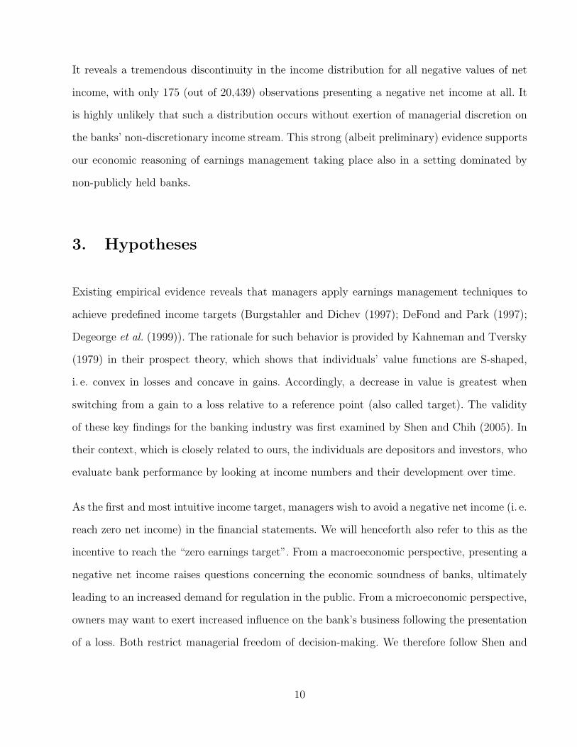
It reveals a tremendous discontinuity in the income distribution for all negative values of net
income, with only 175 (out of 20,439) observations presenting a negative net income at all. It
is highly unlikely that such a distribution occurs without exertion of managerial discretion on
the banks’ non-discretionary income stream. This strong (albeit preliminary) evidence supports
our economic reasoning of earnings management taking place also in a setting dominated by
non-publicly held banks.
3. Hypotheses
Existing empirical evidence reveals that managers apply earnings management techniques to
achieve predefined income targets (Burgstahler and Dichev (1997); DeFond and Park (1997);
Degeorge et al. (1999)). The rationale for such behavior is provided by Kahneman and Tversky
(1979) in their prospect theory, which shows that individuals’ value functions are S-shaped,
i. e. convex in losses and concave in gains. Accordingly, a decrease in value is greatest when
switching from a gain to a loss relative to a reference point (also called target). The validity
of these key findings for the banking industry was first examined by Shen and Chih (2005). In
their context, which is closely related to ours, the individuals are depositors and investors, who
evaluate bank performance by looking at income numbers and their development over time.
As the first and most intuitive income target, managers wish to avoid a negative net income (i. e.
reach zero net income) in the financial statements. We will henceforth also refer to this as the
incentive to reach the “zero earnings target”. From a macroeconomic perspective, presenting a
negative net income raises questions concerning the economic soundness of banks, ultimately
leading to an increased demand for regulation in the public. From a microeconomic perspective,
owners may want to exert increased influence on the bank’s business following the presentation
of a loss. Both restrict managerial freedom of decision-making. We therefore follow Shen and
10

Chih (2005) in arguing that managers have strong incentives to preserve stakeholders’ confidence
in their bank by preventing presentation of a negative net income. Therefore, we hypothesize:
Hypothesis 1 (H1 ). Having a negative net income pre-340f 6 is positively correlated with the
extent of a release of 340f reserves.
Achieving income targets other than zero is certainly relevant to bank managers, too. These may
be set by management announcements or analysts’ reports on the expected future performance
of a bank (McVay (2006)). However, since neither Savings Banks nor Coops are followed by
financial analysts or give precise future earnings announcements, we do not investigate the
effects of explicit announcements any further. A more relevant earnings target is set by the
bank’s performance in the previous accounting period. Accordingly, managers have incentives
for avoiding a drop in net income, which we henceforth also refer to as the incentive to reach
the “zero earnings changes target”. Being mainly relevant to listed German banks, investors
interpret perennial slight increases in net income – particularly if transferred into moderately
rising annual dividends – as a sign of the management’s confidence in future earnings prospects
(Lintner (1956), Benartzi et al. (1997)). Stock prices and thus also the bank’s value are likely
to rise following a consecutive dividend increase. This, in turn, strengthens the management’s
position. By contrast, falling short of the previous period’s earnings level induces investors
(depositors) to turn away from the bank in search of a more profitable (secure) alternative. For
non-listed banks, the rationale for reaching the zero earnings changes target holds for another
reason. As noted by DeFond and Park (1997), achieving at least the previous year’s earnings
level reduces the threat of dismissal or interference by owners, regulators and other stakeholders.
Accordingly, we hypothesize:
6 Henceforth, “net income pre-340f ” refers to net income before consideration of the yearly change in 340freserves, whereas “net income post-340f ” denotes net income as the bottom line of the P&L.
11

Hypothesis 2 (H2 ). Having a net income pre-340f below its own previous year’s income level
is positively correlated with the extent of a release of 340f reserves.
Both the zero earnings and the zero earnings changes targets have been examined extensively
in the past. As one major contribution of this study to the literature, we define (and test)
a third income target by interpreting the prospect theory in a broader sense. Therefore, we
substitute the presented (company-specific) zero earnings changes target by a combination of
an industry with a regional benchmark. In addition to evaluating bank performance with respect
to the previous period’s earnings of the same bank, we believe that stakeholders also take into
account the performance relative to a peer group of banks in the same region (Kanagaretnam
et al. (2003)). Therefore, managers are inclined to avoid a shortfall in net income compared to
a peer group, which we will henceforth also refer to as the “peer group earnings target”.7 Thus,
we hypothesize:
Hypothesis 3 (H3 ). Having a net income pre-340f below the previous year’s income level of
its peer group is positively correlated with the level of a release of 340f reserves.
The final motive to be investigated in this study is not related to reaching any specific income
target. Rather, it refers to earnings management behavior in the course of time. The managerial
objective to present a stable income stream, besides achieving particularly the zero earnings tar-
get, also involves avoiding extremely high levels of net income in years of outstanding economic
well-being. Accordingly, managers consider both current and expected future performance in
terms of unmanaged or non-discretionary income (i. e. income before reserve creation, provi-
sions and taxes). For instance, if current unmanaged income is relatively low (high), but future
unmanaged income is predicted to be relatively high (low), managers may release (build) 340f
reserves. Thus, in times of economic prosperity they “save” income by building 340f reserves to
7 Details on our way of defining the peer group performance are described in Section 4.1.
12

be able to “consume” it during periods of bad performance. Accordingly, managers are inclined
to reduce the variability of the net income of their banks over time. Doing so is supposed to lower
the cost of capital as well as the perceived probability of bankruptcy of financial institutions
(Barth et al. (1995); Kanagaretnam et al. (2004)). Thus, finally, we hypothesize:
Hypothesis 4 (H4 ). A bank’s non-discretionary income is negatively correlated with the extent
of a release of 340f reserves.
4. Empirical analysis
4.1. Data and variables
For our empirical analysis, we use data from the Deutsche Bundesbank’s prudential database
BAKIS for the years 1994 through 2009. BAKIS is the information system on bank-specific data
which is jointly operated by the Deutsche Bundesbank and the German Financial Supervisory
Authority (Memmel and Stein (2008)). The database contains information on the financial
statements and supervisory reports of individual German banks, and is therefore unique. Our
initial sample consists of 40,870 observations from 5,377 banks8 for the years 1994 through 2009.
Due to a lack of values in important variables used in our analysis, we lose 10,351 observations.
Moreover, due to first differencing of some of the variables and using second lags of our variables
in our dynamic panel data estimations requires us to neglect a further 10,080 observations.
Therefore, our final panel dataset consists of 20,439 observations of 3,643 banks.
8 This figure is higher than the actual number of existing banks because, in the case of (frequently occurring)mergers, we, technically speaking, created a new bank independent of the merging ones. This new bankstarts operating in the year of the merger.
13

We analyze unconsolidated accounts prepared according to HGB, which is appropriate because
the vast majority of banks in our sample (primarily referring to Savings Banks and Coops)
do not prepare consolidated accounts at all, and the unconsolidated ones are used to evaluate
management performance as well as to determine managerial compensation.
In most parts of our analysis we divide the German banking market into three different cate-
gories: Coops, Savings Banks and Commercials. We exclude other types of financial institutions
such as home loan banks, mortgage banks or securities trading banks because they either do
not meet the definition of a bank according to section 1 of the German Banking Act or they
do not conduct core banking business such as lending and borrowing.
Table 1 gives detailed information on the number of banks observed in our final panel and
the split between bank categories by year. Our sample is clearly dominated by Coops, whereas
Savings Banks and particularly Commercials are – in terms of numbers – of only minor impor-
tance. The fact that the number of observations in each category is considerably smaller at the
end than at the beginning of our sample period reveals persistently high numbers of mergers
(particularly within Savings Banks and Coops) in the German banking market.
Table 2 reveals the number of banks using 340f reserves and how this use changes over time.
“Use” in this context means that an observation either holds a positive level of 340f reserves
at year-end, or it released its total amount of 340f reserves that existed at the beginning of
the year. The main conclusions to be drawn from Table 2 are threefold. First, more than 99%
of banks in our sample make use of 340f reserves. Second, those using them much more often
increase or leave the level of existing reserves unchanged rather than releasing it. Third, the
share of banks releasing 340f reserves reaches peaks in 2000 and, in particular, in 2008. The
latter peak is conclusively explained by banks trying to counterbalance adverse effects on their
returns caused by the financial crisis. However, the peak in 2000 is somewhat surprising and
14

Coops Savings Banks Commercials Total
Year No. Row% No. Row% No. Row% No. Col.%
1997 1,750 76.19 513 22.33 34 1.48 2,297 11.241998 1,637 74.21 536 24.30 33 1.50 2,206 10.791999 1,421 71.91 525 26.57 30 1.52 1,976 9.672000 1,131 67.77 501 30.02 37 2.22 1,669 8.172001 989 66.29 462 30.97 41 2.75 1,492 7.302002 917 65.64 434 31.07 46 3.29 1,397 6.832003 886 67.33 391 29.71 39 2.96 1,316 6.442004 915 68.85 375 28.22 39 2.93 1,329 6.502005 957 70.99 359 26.63 32 2.37 1,348 6.602006 1,001 71.60 363 25.97 34 2.43 1,398 6.842007 1,020 73.07 342 24.50 34 2.44 1,396 6.832008 1,006 73.11 339 24.64 31 2.25 1,376 6.732009 936 75.54 276 22.28 27 2.18 1,239 6.06
Total 14,566 71.27 5,416 26.50 457 2.24 20,439 100.00
Table 1: Number of observations in the panel by bank category and year.
Note: Savings Banks (Coops) contains local savings as well as “Landesbanken” (local cooperative banks and cooperative centralinstitutions). Commercials comprises privately held and regional banks as well as the German money-center banks. “No.” gives thenumber of observations in our panel by category and year. “Row%” reveals the share of each bank category on the overall numberof observations in our panel by year. “Total No.” displays the overall number of observations by year. “Total Col.%” gives the shareof observations by year on the overall number of observations in our panel by year.
potentially due to early reactions to the turmoil caused by the bursting of the dotcom bubble
at the turn of the millennium.
To analyze earnings management behavior by means of 340f reserves, we use REL 340f RESi ,t ,
which is the release of 340f reserves of bank i at the end of year t as percent of their beginning-of-
year t level, as the dependent variable in all our regression models. Scaling by the beginning-of-
year level of these reserves (rather than by total assets as used for many other variables) is most
appropriate to clearly capture the strengths of underlying earnings management incentives. A
negative value of this variable means that a bank has built (instead of released) 340f reserves in
the corresponding year. If, by contrast, REL 340f RESi ,t has a positive value, the binary variable
D REL 340fi ,t equals 1, and 0 otherwise.
Regarding H1 (referring to the zero earnings target), D LOSSi ,t is a binary variable which
equals 1 if bank i in year t has a negative net income pre-340f, and 0 otherwise. It is worth
15

of which of which
Use of 340f Release Increase No changeYear Obs. No. Row. % No. Row. % No. Row. % No. Row. %
1997 2,297 2,285 99.48 165 7.22 1,563 68.40 557 24.381998 2,206 2,189 99.23 163 7.45 1,461 66.74 565 25.811999 1,976 1,968 99.60 218 11.08 1,256 63.82 494 25.102000 1,669 1,657 99.28 229 13.82 1,037 62.58 391 23.602001 1,492 1,479 99.13 173 11.70 1,064 71.94 242 16.362002 1,397 1,385 99.14 153 11.05 1,070 77.25 162 11.702003 1,316 1,310 99.54 126 9.62 1,015 77.48 169 12.902004 1,329 1,322 99.47 63 4.77 1,133 85.70 126 9.532005 1,348 1,341 99.48 45 3.36 1,160 86.50 136 10.142006 1,398 1,392 99.57 54 3.88 1,217 87.43 121 8.692007 1,396 1,394 99.86 129 9.25 988 70.88 277 19.872008 1,376 1,374 99.85 298 21.69 809 58.88 267 19.432009 1,239 1,235 99.68 26 2.10 1,130 91.50 79 6.40
Total 20,439 20,331 99.47 1,842 9.06 14,903 73.30 3,571 17.64
Table 2: Activities regarding 340f reserves over time.
Note: “Obs.” contains the overall number of observations in our panel by year. “Use of 340f” reveals the number of observations(“No.”) as well as the percentage in relation to the overall number of observations in our panel (“%”) that use 340f reserves by year.“Use” in this context means that an observation is either holding a positive level of 340f reserves at year-end, or it released its totalamount of 340f reserves existing at the beginning of the year. “Release” gives the number of observations that release 340f reservesby year as well as the percentage of observations doing so. Please note that this and the following percentages are calculated inrelation to the observations using 340f reserves (rather than to the overall number of observations) by year. “Increase” reports thenumber (as well as the percentage) of observations that increase their level of 340f reserves by year. “No change” gives the number(as well as the percentage) of observations that did not change their level of 340f reserves by year.
16

noting that all target-related binary variables equal 1 if the target is achieved, but not exceeded.
Accordingly, D LOSSi ,t is 1 if net income pre-340f < 0 and 0 if net income pre-340f ≥ 0.
Regarding H2 (addressing the zero earnings changes target), D PREVi ,t is a binary variable
which equals 1 if bank i in year t has a net income pre-340f below its own previous year’s level,
and 0 otherwise.
With respect to H3 (referring to the peer group earnings target), D PEERi ,t equals 1 if bank
i in year t has a net income pre-340f (as percent of total assets) below the average previous
year’s level (scaled by mean total assets) of its peer group, and 0 otherwise. We use the previous
period’s peer group income as the best available estimate of current performance, since con-
temporaneous information on the performance of peer group banks is not usually available to a
competitor’s management. We define the relevant peer group differently for different categories
of banks in our sample. For Coops and Savings Banks, we consider the peer group as being all
banks located in the same administrative district (“Regierungsbezirk”), regardless of which of
the two categories an observation belongs to. Using this definition also for Commercials would
(probably) not adequately capture their relevant peer groups, because these banks frequently
operate nationwide. Therefore, we determine the peer group for Commercials as being all banks
in this category. We are aware that both ways of defining a peer group can only crudely capture
actual managerial behavior, because managers presumably take the precise income levels of one
or two close-by banks rather than the average income level of all banks in their peer group as
their relevant benchmark. However, from our point of view the approach taken here is the best
way to proxy existing peer group pressure.
17

With respect to H4 (addressing a reduction in the income variability over time), NIBRPTTAi ,t
is defined as the non-discretionary income (i. e. income before reserves’ creation, provisions and
taxes)9 of bank i at the end of year t as percent of its beginning-of-year t total assets.10
We take into account a potential use of 340f reserves for regulatory capital management in two
alternative ways. First, banks may release 340f reserves to indirectly enhance their following
period’s tier 1 capital ratio. Releasing these reserves increases net income, which in turn raises
the following period’s equity, particularly if large parts of net income are retained rather than
distributed to the owners in the corresponding year. Since equity is acknowledged as tier 1
capital, the corresponding ratio rises. Second, banks may try to directly enhance their tier 2
capital by increasing 340f reserves. We use CHTIER1i ,t (CHTIER2i ,t) as the change in the
level of tier 1 (tier 2) capital of bank i from year t− 1 to t as percent of its beginning-of-year
t risk-weighted assets to account for both effects,11 and we expect to see a negative (positive)
correlation with REL 340f RESi ,t .
Besides variables necessary for detecting managerial discretion, we have to take into account
the risk provisioning function of 340f reserves. We follow Lobo and Yang (2001) and others in
using a broad set of risk-related variables. We include CHCLTAi ,t , which is the change in the ratio
of customer loans to total assets of bank i from year t− 1 to t as percent of beginning-of-year
t total assets. This variable measures changes in credit risk arising from an expansion of the
loan portfolio. Therefore, we expect to see a negative association with a release in 340f reserves.
LLATAi ,t−1 is the level of the loan loss allowance of bank i at the end of year t − 1 as percent
of its end-of-year t − 1 total assets. The loan loss allowance (as the accumulation of LLP of
9 A similar definition of non-discretionary income is commonly used. However, since 340f reserves are nottax-deductible, taxes in our case could arguably be added to this non-discretionary income number.
10 In line with most previous studies, we consistently scale all flow variables by the beginning-of-year value ofthe corresponding denominator, whereas for all stock variables the end-of-year value of the correspondingyear is used. This prevents potential problems of endogeneity.
11 The yearly change in 340f reserves is excluded from tier 2 capital to prevent endogeneity.
18

the preceding periods) represents ex-post credit risks, for which provisions ideally have already
been built. Therefore, most studies on the use of LLP assume a negative correlation between
this variable and risk provisions. However, the fact that 340f reserves are meant to account for
risks more generally than LLP may cause the correlation with REL 340f RESi ,t to be negligible.
Moreover, we include LLPTAi ,t , which is the amount of specific LLP built by bank i throughout
year t as percent of its beginning-of-year t total assets. The use of LLP for earnings manage-
ment revealed in many previous studies gives rise to simultaneity concerns between LLPTAi ,t
and REL 340f RESi ,t . To adequately address these, we apply a dynamic generalized method of
moments estimation technique (Blundell and Bond (1998)) with Windmeijer (2005) correction.
Doing so enables us to instrument the association between LLPTAi ,t and REL 340f RES
i ,t with the
help of an exogenous variable. A “good” instrument should be relevant and valid at the same
time (Baum et al. (2003)), meaning that it should be correlated with the endogenous regressor
(LLPTAi ,t ), while being orthogonal to the residuals of the regression. Whereas the former condi-
tion is easily verifiable by looking at the correlation between the endogenous and the instrument
variable, the latter is subject to thoughtful economic considerations.
We are confident that CHNPLi ,t , which is the change in the non-performing loans of bank i
from year t − 1 to t as percent of its beginning-of-year t volume of customer loans,12 satisfies
both conditions for being an adequate instrument. First, the correlation of this NPL ratio with
LLP is usually found to be strong (Kanagaretnam et al. (2004); Adams et al. (2009)), since
LLP are built for each loan that is classified as non-performing. Table 6 confirms this for our
sample at a considerable level of 0.4415. If banks already react to changes in non-performing
loans by adjusting their LLP, there is no need to further provision for these by means of 340f
12 Loans are non-performing if the payment of principal or interest is overdue by at least 90 days.
19

reserves. Therefore, we quite reasonably believe the orthogonality condition between CHNPLi ,t
and REL 340f RESi ,t to hold.13
To account for 340f reserves potentially being used as provisions for market risk exposure, we
include CHOBSTAi ,t , which is the change in off-balance sheet activities of bank i from year t− 1
to t as percent of its beginning-of-year t total assets.
As a measure not directly related to any of the risk types, we add ZSCOREi ,t to our regression
models. This z-score is calculated as the ratio of capital and profits of bank i at the end of year t
to the standard deviation of profits of bank i over time, each position measured relative to total
assets of bank i (Boyd et al. (1993)).14 A higher z-score implies that the bank is more stable,
i. e. the bank is further from insolvency. It is frequently used as a general measure of future
default risk for banks (e. g. Onali (2010)). It is particularly appealing in our setting because it
relies solely on accounting measures without requiring stock return data.
As the level of 340f reserves is restricted to 4% of the valuation basis, we include LIM BASISi ,t ,
which is the amount of existing 340f reserves of bank i at the end of year t (before considering
the yearly change therein) as percent of its beginning-of-year t valuation basis. For banks close
to the limit, a release decision may primarily be driven by the aim of retaining managerial
freedom of decision-making with respect to 340f reserves in the future. LNTAi ,t is the natural
logarithm of total assets of bank i at the end of year t. This variable is included since it is used
as a control in many earnings management studies, and partly found to be significant (Alali
and Jaggi (2010)). Finally, we add CRGDP t, which is the aggregate volume of bank lending
13 Any indirect association between those two variables (e. g. through the relation between LLPTAi,t and
LLATAi,t−1
) does not impair this orthogonality condition and thus the validity of the instrument.14 Its quality largely depends on the availability of a long time series in the panel dataset from which the
standard deviation of profits is derived. Due to our unbalanced panel, we limit the calculation of thestandard deviation of ROA in the denominator of the z-score to the 1st and 99th percentile for all banks.The calculation of the bounds is done by bank category (Savings Banks, Coops and Commercials) andonly banks for which a time series of at least seven years is available are taken into account.
20

to the economy (in real terms) in year t as percent of real gross domestic product in year t.
This is also known as the “credit over GDP” ratio and it is meant to control for the state of
the business cycle and its effects on our dependent variable. We provide comprehensive variable
descriptions in Table 3.
A relatively moderate outlier treatment is applied to the dataset. We winsorize all non-binary
variables (that have not been winsorized in other ways) at the 0.5% and 99.5% quantile. Table
4 provides descriptive statistics for all non-binary variables.
4.2. Descriptive statistics
As part of our descriptive statistics, we have in Figure 1 already provided evidence of the
existence of earnings management in the German banking market, which is dominated by
non-listed institutions. We proceed by graphically revealing the relevance of 340f reserves in
German banks. Therefore, Figure 2 shows a histogram of the level of 340f reserves as percent
of the valuation basis. Apparently, the majority of observations holds 340f reserves at about
1% of the valuation basis. However, a large number exceeds this level by far, with roughly 100
observations reaching the upper limit of 4%. Considering that an average (German) bank holds
equity at about 5% of total assets, this corroborates the importance of 340f reserves for German
banks already revealed in Table 2.
Figure 3 displays a histogram of REL 340f RESi ,t , for reasons of visibility excluding those 3,586
(115) observations with a zero change in 340f reserves (a value of a release smaller than -200%).
It supports Table 2 in revealing that building 340f reserves occurs more frequently (and to a
larger extent) than releases therein.
21

Variable Description
REL 340f RESi,t Release of 340f reserves of bank i at the end of year t as % of their beginning-of-year t level.
REL 340f RESi,t−1
Release of 340f reserves of bank i at the end of year t− 1 as % of their beginning-of-year t− 1 level.
REL 340f RESi,t−2
Release of 340f reserves of bank i at the end of year t− 2 as % of their beginning-of-year t− 2 level.
D REL 340f i,t Binary variable equaling 1 if bank i in year t has a releease in 340f reserves, and 0 otherwise.
D NOLOSSi,t Binary variable equaling 1 if bank i in year t has a positive net income pre-340f, and 0 otherwise.D LOSS i,t Binary variable equaling 1 if bank i in year t has a negative net income pre-340f, and 0 otherwise.D LOSS−i,t Binary variable equaling 1 if bank i in year t has a negative net income pre-340f, and is unable to
reach the zero net income post-340f even by releasing all of its 340f reserves, and 0 otherwise.D LOSS+i,t Binary variable equaling 1 if bank i in year t has a negative net income pre-340f, but is able to reach
zero net income post-340f by releasing its 340f reserves, and 0 otherwise.
D NOPREV i,t Binary variable equaling 1 if bank i in year t has a net income pre-340f above its own previous year’snet income level post-340f, and 0 otherwise.
D PREV i,t Binary variable equaling 1 if bank i in year t has a net income pre-340f below its own previous year’snet income level post-340f, and 0 otherwise.
D PREV−i,t Binary variable equaling 1 if bank i in year t has a net income pre-340f below its own previous year’snet income post-340f, and is unable to reach zero net income changes post-340f even by releasing allof its 340f reserves, and 0 otherwise.
D PREV+i,t Binary variable equaling 1 if bank i in year t has a pre-340f net income below its own previous year’snet income (post-340f), but is able to reach zero net income changes post-340f by releasing its 340freserves, and 0 otherwise.
D NOPEERi,t Binary variable equaling 1 if bank i in year t has a net income pre-340f (as % of its beginning-of-yeart total assets) above the average previous year’s post-340f income level of its peer group (as % ofmean total assets), and 0 otherwise.
D PEERi,t Binary variable equaling 1 if bank i in year t has a net income pre-340f (as % of its beginning-of-yeart total assets) below the average previous year’s post-340f income level of its peer group (as % ofmean total assets), and 0 otherwise.
D PEER−i,t Binary variable equaling 1 if bank i in year t has a net income pre-340f (as % of its beginning-of-year ttotal assets) below the average previous year’s post-340f income level of its peer group (as % of meanbeginning-of-year t − 1 total assets), and is unable to reach the peer group income level post-340feven by releasing all of its 340f reserves, and 0 otherwise.
D PEER+i,t Binary variable equaling 1 if bank i in year t has a net income pre-340f (as % of its beginning-of-yeart total assets), but is able to reach the peer group income level post-340f by releasing its 340f reserves,and 0 otherwise.
NIBRPTTAi,t Non-discretionary income (i. e. income before reserves’ creation, provisions, and taxes) of bank i in
year t as % of its beginning-of-year t total assets.
CHTIER1RWAi,t Change in the level of tier 1 capital of bank i from year t − 1 to t as % of its beginning-of-year t
risk-weighted assets.CHTIER2RWA
i,t Change in the level of tier 2 capital of bank i from year t − 1 to t (net of changes in 340f reserves)as % of its beginning-of-year t risk-weighted assets.
CHCLTAi,t Change in the ratio of customer loans to total assets of bank i from year t−1 to t as % of beginning-
of-year t total assets.LLPTA
i,t Amount of specific LLP built by bank i throughout year t as % of its beginning-of-year t total assets.
LLATAi,t−1
Level of the loan loss allowance of bank i at the end of year t− 1 as percent of its end-of-year t − 1total assets.
CHNPLi,t Change in the non-performing loans of bank i from year t − 1 to t as % of its beginning-of-year t
volume of customer loans.CHOBSTA
i,t Change in off-balance sheet activities of bank i from year t − 1 to t as % of its beginning-of-year t
total assets.ZSCORE i,t Ratio of capital and profits of bank i at the end of year t to the standard deviation of profits of bank
i over time, each position measured relative to total assets of bank i.
LIMBASISi,t Level of existing 340f reserves of bank i at the end of year t (before considering the yearly change
therein) as % of its beginning-of-year t valuation basis.LNTAi,t Natural logarithm of total assets of bank i at the end of year t.CRGDPi,t Aggregate volume of bank lending to the economy (in real terms) in year t as % of real gross domestic
product in year t.
Table 3: Short description of variables.
22

Variable Category Mean Std. Dev. p1 p50 p99
Coops 0.41 2.85 0.02 0.14 3.24Total assets (in billion euro) Savings Banks 3.23 11.27 0.15 1.15 57.56
Commercials 8.28 21.56 0.09 1.52 137.91
Coops -16.18 39.71 -162.03 -9.98 73.01REL 340f RES
i,t (in %) Savings Banks -11.76 29.65 -114.29 -8.23 71.06Commercials -8.90 45.67 -200.94 0.00 100.00
Coops 0.77 0.59 -0.94 0.78 2.36NIBRPTTA
i,t (in %) Savings Banks 0.67 0.51 -0.71 0.69 1.79Commercials 0.74 0.99 -1.48 0.62 3.10
Coops 0.27 0.93 -1.65 0.15 3.77
CHTIER1RWAi,t (in %) Savings Banks 0.24 0.88 -1.33 0.13 3.78
Commercials 0.24 1.69 -2.86 -0.01 4.53
Coops 0.14 0.97 -2.69 0.06 3.21
CHTIER2RWAi,t (in %) Savings Banks 0.11 0.87 -2.30 0.06 2.58
Commercials 0.04 1.07 -3.51 0.00 3.50
Coops -0.12 2.87 -7.29 -0.17 7.41CHCLTA
i,t (in %) Savings Banks -0.03 2.29 -5.93 -0.06 5.94Commercials -0.15 4.67 -10.56 -0.16 9.65
Coops 1.63 1.10 0.08 1.41 5.36LLATA
i,t−1 (in %) Savings Banks 1.79 1.05 0.22 1.63 5.23Commercials 2.45 1.87 0.04 2.12 7.27
Coops 0.02 0.47 -1.30 0.02 1.41LLPTA
i,t (in %) Savings Banks 0.02 0.39 -1.04 0.02 1.09Commercials 0.02 0.86 -2.96 0.04 2.69
Coops 0.05 1.93 -4.50 -0.08 6.12CHNPLi,t (in %) Savings Banks 0.01 1.38 -3.63 -0.10 4.10
Commercials 0.24 3.49 -6.57 -0.07 12.51
Coops -0.05 1.93 -5.54 -0.11 5.70CHOBSTA
i,t (in %) Savings Banks -0.03 2.06 -5.82 -0.12 9.36Commercials -0.52 3.40 -9.35 -0.20 8.78
Coops 28.39 13.78 7.80 25.47 73.69ZSCOREi,t Savings Banks 24.05 11.31 6.59 21.63 64.25
Commercials 16.73 11.19 5.55 14.79 59.35
Coops 1.36 0.89 0.12 1.14 3.71LIMBASIS
i,t (in %) Savings Banks 1.58 0.91 0.08 1.48 3.61Commercials 1.40 0.90 0.08 1.20 3.68
Table 4: Descriptive statistics for non-binary variables by bank category.
Note: Values given here are based on those observations that use 340f reserves (also see Table 2) only. Savings Banks contains allsavings banks as well as “Landesbanken”. Coops consists of all cooperative banks, including the cooperative central institutions.Commercials contains all privately held and regional banks as well as the German money-center banks. “No.” denotes the numberof observations in our panel per category. “Mean” (“Std. dev.”) describes the mean (standard deviation) of each variable across allobservations in each category. “Total assets” refers to total assets. For comprehensive variable descriptions see Table 3.
23

050
100150
200Fre
quency
0% 1% 2% 3% 4%
Figure 2: Level of 340f reserves as % of valuation basis.
Note: The distribution interval width is chosen as 0.02%. “Frequency” refers to the number of observations in each interval. Thevaluation basis (as the denominator) comprises customer and interbank loans as well as bonds, other fixed-income securities, sharesand securities bearing variable interest that at the same time are designated to the “liquidity reserve” (also see Section 2.1).
0200
400600
800100
0Fre
quency
−200% −100% 0% 100%
Figure 3: Release of 340f reserves as % of their beginning-of-year level.
Note: The distribution interval width is chosen as 1%. “Frequency” refers to the number of observations in each interval. For reasonsof visibility, we neglect 3,586 (115) observations with a zero change in 340f reserves (a release smaller than -200%, i. e. an increasein the level of 340f reserves by more than 200%) of their previously existing level.
24

Figure 4 contrasts the variability of net income pre- compared to post-340f. The left-hand
boxplot presents the standard deviation of net income pre-340f, whereas that on the right-
hand side exhibits the standard deviation of net income post-340f, both as percent of mean
total assets.15 As the major conclusion to be drawn from this figure, the median as well as the
upper and the lower quartile in the right-hand boxplot are located well below the ones on the
left. Thus, by managing their 340f reserves correspondingly, banks are apparently successful in
reducing the variability of their net income to a large extent. This provides support for H4.
Note also that the interquartile range shrinks from roughly 0.0025% in the left-hand boxplot to
0.0010% on the right, meaning that by using 340f reserves all banks are moving closer to one
another with respect to the standard deviation of net income.
0.002%
0.004%
0.006%
0.008%
0.01%
0%Std
. dev. o
f net in
come (p
re−340
f) as %
of me
an tota
l asset
s
0.002%
0.004%
0.006%
0.008%
0.01%
0%Std
. dev. o
f net in
come (p
ost−34
0f) as
% of m
ean tot
al asse
ts
Figure 4: Standard deviation of net income pre- and post-340f.
Note: For reasons of visibility, values outside the upper and lower whisker in each boxplot are neglected. Standard deviations arecalculated using all observations in the sample. To enhance reliability of the standard deviations used, we reproduced this graphusing only standard deviations of banks with at least eight observations in the panel. The results remain unchanged.
To investigate the relevance of the earnings benchmarks as hypothesized in H1, H2 and H3, we
proceed by conducting contingency analyses on the relationship between the benchmark-related
binary variables and releases of 340f reserves. Such analyses test independence between two or
more categorical variables. A corresponding chi-squared test investigates the null hypothesis
15 To enhance the reliability of this figure, we reproduced both boxplots using only banks with at least eightobservations in the panel. We find the results to be stable.
25

that rows and columns of the contingency table are independent in a statistical sense. This
should be the case if none of the two variables under consideration is influenced by the other.16
Table 5 relates the binary variable D REL 340fi ,t to D LOSS i,t in Panel A (referring to H1 ),
to D PREV i,t in Panel B (H2 ), and to D PEERi,t in Panel C (H3 ).
Panel A: D LOSSi,t Panel B: D PREVi,t Panel C: D PEERi,t
Total0 1 0 1 0 1 (by panel)
DREL340f i,t
0Frequency 18,426 63 15,166 3,323 14,296 4,193 18,489Row% 99.66 0.34 82.03 17.97 77.32 22.68 100.00Col% 96.19 5.36 99.40 65.49 99.28 70.68 90.94
1Frequency 730 1,112 91 1,751 103 1,739 1,842Row% 39.63 60.37 4.94 95.06 5.59 94.41 100.00Col% 3.81 94.64 0.60 34.51 0.72 29.32 9.06
Total 19,156 1,175 15,257 5,074 14,399 5,932 20,331Row% 94.22 5.78 75.04 24.96 70.82 29.18 100.00Col% 100.00 100.00 100.0 100.00 100.0 100.0 100.00
Panel A/B/C: Pearson chi2 = 1.1e+04/5.3e+03/4.2e+03; Pr = 0.000/0.000/0.000
Table 5: Contingency table on D REL 340fi ,t and the benchmark-related variables.
Note: The table shows contingency analyses on D REL 340fi,t with D LOSSi,t , D PREVi,t and D PEERi,t . For comprehensivevariable descriptions, see Table 3. “Row%” (by panel) gives the share of observations in each field on the overall number ofobservations in each row. “Col%” gives the share of observations in each field on the overall number of observations in each column.The given values of the chi-squared test at the bottom (investigating independence of rows and columns of the contingency table)strongly indicate these to be independent.
Panel A relates D REL 340fi ,t to D LOSS i,t. It is striking that a majority of 94.64% (only
a minority of 3.81%) of observations failing (managing) to reach the zero earnings target, i. e.
having D LOSS i,t = 1, release reserves. Moreover, 60.37% of observations releasing 340f reserves
miss this target pre-340f.17 These findings clearly support H1. With respect to H2, Panel B
relates D REL 340fi ,t to D PREV i,t. 34.51% (0.58%) of observations that fail (manage) to
reach the zero earnings changes target have a release of 340f reserves. Furthermore, 95.06% of
16 For further details on contingency analysis, see Agresti (2007).17 It is important to note that this table does not allow to derive any statement on whether these observations
reached this target post-340f.
26

observations releasing 340f reserves miss this target before doing so. Both outcomes strongly
support H2. Finally, Panel C refers to H3 and relates D REL 340fi ,t to D PEERi,t. 29.32%
(0.72%) of the observations that fail (manage) to reach the peer group income target release 340f
reserves. Additionally, 94.41% of observations releasing 340f reserves miss the corresponding
target pre-340f. Thus, H3 is strongly supported, too.
To corroborate our bivariate results by controlling for bank-specific conditions as well as effects
caused by the business cycle, we now turn to our multivariate analysis. Table 6 reports the
correlation coefficients among all variables used in the following regressions. With only four
correlations exceeding the level of 0.4, correlation among regressors is generally below levels
in which multicollinearity would be a serious problem. All correlations between the depen-
dent variable (REL 340f RESi ,t ) and the earnings-related ones are in line with our hypothesized
expectations. Therefore, we refrain from commenting on Table 6 in more detail.
27

REL D D D NIB CH CH CH
340f RESi,t LOSS i,t PREV i,t PEERi,t RPTTA
i,t TIER1 i,t TIER2 i,t CLTAi,t LLATA
i,t−1
REL 340f RESi,t 1.0000
D LOSS i,t 0.3379 1.0000D PREV i,t 0.3412 0.4246 1.0000D PEERi,t 0.3268 0.3845 0.5602 1.000
NIBRPTTAi,t -0.2231 -0.2830 -0.2692 -0.3915 1.0000
CHTIER1RWAi,t 0.0391 0.0541 0.0789 0.0162 -0.1485 1.0000
CHTIER2RWAi,t 0.2205 0.1555 0.1578 0.1349 -0.1584 0.3781 1.0000
CHCLTAi,t 0.0475 -0.0076 0.0193 0.0139 0.0416 -0.1699 -0.0216 1.0000
LLATAi,t−1
-0.0410 0.0678 0.0022 0.0565 -0.1606 -0.0162 -0.0236 -0.0875 1.0000
LLPTAi,t 0.1765 0.2241 0.1988 0.1736 0.5064 -0.0968 0.0111 0.0449 -0.1415
CHNPLi,t 0.1346 0.1603 0.1246 0.0937 0.1753 -0.0343 -0.0164 -0.0373 -0.1072CHOBSTA
i,t -0.0297 -0.0240 -0.0240 -0.0212 0.0603 -0.0504 -0.0255 0.0587 -0.0304
ZSCOREi,t -0.0351 -0.1868 -0.1386 -0.1930 0.1097 0.1067 0.0436 -0.0245 -0.1711
LIMBASISi,t 0.1692 -0.0181 -0.0737 -0.1470 0.0593 0.1920 0.1445 -0.0655 -0.0292
LNTAi,t 0.0083 0.0293 -0.0298 0.0945 -0.1299 0.0247 -0.0217 -0.0638 0.0881CRGDP i,t -0.0797 0.0152 -0.0488 -0.0813 0.0392 -0.1800 -0.1082 0.0587 0.0396REL 340f RES
i,t−10.2303 0.0605 0.0552 0.0635 -0.0368 0.0038 -0.2559 -0.0186 -0.0124
REL 340f RESi,t−1
-0.0028 -0.0099 -0.0006 0.0006 -0.0051 0.0023 -0.0060 0.0050 -0.0075
CH CH Z REL REL
LLPTAi,t−1
NPLi,t OBSTAi,t SCOREi,t LIMBASIS
i,t LNTAi,t CRGDP i,t 340f RESi,t−1
340f RESi,t−2
LLPTAi,t 1.0000
CHNPLi,t 0.4338 1.0000CHOBSTA
i,t -0.0080 -0.0253 1.0000
ZSCOREi,t -0.0896 -0.0373 0.0284 1.0000
LIMBASISi,t -0.1007 0.0207 -0.0081 0.1706 1.0000
LNTAi,t -0.0450 -0.0117 -0.0009 -0.0242 0.0590 1.0000CRGDP i,t 0.0757 0.0390 -0.1349 -0.1324 -0.1959 -0.0114 1.0000
REL 340f RESi,t−1
0.0414 0.0587 -0.0072 -0.0051 0.0924 0.0167 0.0179 1.0000
REL 340f RESi,t−2
-0.0095 -0.0009 0.0160 0.0014 0.0006 -0.0001 0.0184 0.0177 1.0000
Table 6: Correlations.
Note: Pearson’s correlation coefficients are reported. For comprehensive variable descriptions, see Table 3.
28

4.3. Multivariate analysis
4.3.1. Research design
Our multivariate results on the impact of different earnings-related variables on releases of
340f reserves are derived from a dynamic generalized method of moments estimation technique
(Blundell and Bond (1998)) with Windmeijer (2005) correction. We use REL 340fRESi,t as the
dependent variable, and two of its lags are used as regressors since second-order autocorrelation
is present in the data. Doing so also accounts for the potential existence of unobservable bank-
individual effects. We are primarily interested in the results of the earnings-related variables
D LOSS i,t (referring to H1 ), D PREV i,t (H2 ), D PEERi,t (H3 ), and NIBRPT TAi,t (H4 ). We
apply the Hansen test of overidentifying restrictions (Arellano and Bond (1991); Blundell and
Bond (1998)) to assess the validity of our instruments. As this test may be weakened by many
instruments (Roodman (2009)), we use only a very limited set of instruments. Moreover, we
use the same lag structure in all our model specifications. The formal design of the models of
block A (see Table 7) is given in equation (1):
REL 340fRESi,t = β0i + β1 · D LOSSi ,t + β2 · D PREVi ,t + β3 ·D PEERi ,t
+β4 · NIBRPTTAi ,t + β5 · CHTIER1i ,t + β6 · CHTIER2i ,t
+β7 · CHCLTAi ,t + β8 · LLAi ,t−1 + β9 · LLPi ,t + β11 · CHOBSTA
i ,t
+β12 · ZSCOREi ,t + β13 · LIMBASISi ,t + β14 · LNTAi ,t
+β15 · CRGDPi ,t + β16 · REL 340f RESi ,t−1
+β17 · REL 340f RESi ,t−2 + ǫi,t.
(1)
Including two lags of the dependent variable follows Bikker and Metzemakers (2005), who
assume a gradual adjustment of LLP due to a lagged availability of information on the optimal
level of provisions. Thus, we conjecture changes in 340f reserves to adjust gradually over time.
29

4.3.2. Analysis disregarding strength of earnings management incentives
To begin with, we estimate equation (1) on a sample containing banks from all categories
(henceforth: full sample). The estimated coefficients and standard errors (in brackets below
the coefficients) are shown in the second column of Table 7 (Model A.1). Following up, we
split our sample according to the categories introduced in Section 2.2 and estimate equation 1
separately for each category. Results for Coops are contained in Model A.2, those for Savings
Banks in A.3 and those for Commercials in A.4. The tests of overidentifying restrictions as
well as autocorrelation for all models indicate that the instruments used are valid and that we
adequately controlled for second-order autocorrelation.
The results on the full sample (Model A.1) reveal a strongly significant18 and positive asso-
ciation of D LOSS i,t (β1 = 14.443) with REL 340fRESi,t . This confirms our bivariate results
regarding H1, because it indicates that banks missing the zero earnings target release 340f re-
serves to a larger extent than those who succeed in reaching this target. Second, the coefficient
on D PREV i,t (β2 = 5.579) shows that missing the zero earnings changes target (i. e. having
a pre-340f net income below the previous year’s level as the bottom line of the P&L) is also
strongly significantly correlated with a release of 340f reserves. Supporting H2, bank managers
indeed try to avoid a drop in net income by adjusting the level of 340f reserves correspondingly.
Third, the positive and strongly significant coefficient on D PEERi,t (β3 = 6.382) reveals that
missing the peer group earnings target is positively associated with a release of 340f reserves
as well. Backing H3, banks with a net income pre-340f below the previous year’s average net
income of their peer group release 340f reserves to a larger extent than banks which already
reached this target pre-340f. The negative and strongly significant coefficient of the last of our
earnings management-related variables, NIBRPTTAi,t (β4 = -17.574), is in line with our expec-
18 We refer to results being “strongly significant” (“significant’ and “weakly significant”, respectively) if thecorresponding level of significance is 1% (5% and 10%, respectively).
30

dependent variable: REL 340fRESi,t
A.1 A.2 A.3 A.4indep. var. Exp. (All categories) (Coops) (Savings Banks) (Commercials)
D LOSSi,t + 14.443*** 9.030*** 20.791*** 45.661***(1.854) (2.523) (3.064) (10.370)
D PREVi,t + 5.579*** 4.540*** 7.129*** 9.370***(0.603) (0.606) (1.356) (3.611)
D PEERi,t + 6.382*** 7.518*** 4.448*** 1.391(0.776) (0.858) (1.411) (5.471)
NIBRPTTAi,t − -17.574*** -20.294*** -13.497*** -4.776
(1.451) (1.431) (1.777) (6.133)CHTIER1RWA
i,t − -5.256*** -6.080*** -4.067*** -2.734**
(0.309) (0.392) (0.527) (1.378)CHTIER2RWA
i,t + 11.545*** 12.830*** 7.542*** 12.174***
(0.553) (0.666) (0.934) (4.003)
CHCLTAi,t − 0.349*** 0.380*** 0.206 0.225
(0.089) (0.105) (0.145) (0.382)LLATA
i,t−1? -1.112*** -1.300*** -1.027*** 0.660
(0.302) (0.372) (0.366) (1.181)LLPTA
i,t + 20.840*** 23.327*** 16.037*** 5.735
(1.394) (1.453) (2.042) (5.474)CHOBSTA
i,t − -0.101 -0.121 0.094 0.356
(0.102) (0.135) (0.140) (0.325)ZSCOREi,t ? 0.063*** 0.104*** 0.040 0.107
(0.018) (0.023) (0.035) (0.140)
LIMBASISi,t + 7.768*** 8.941*** 6.355*** 4.242
(0.431) (0.568) (0.750) (3.562)LNTAi,t ? -0.714*** -1.275*** -1.220*** -1.188
(0.179) (0.316) (0.423) (1.779)CRGDPt − -0.111*** -0.076** -0.069** -0.135
(0.018) (0.033) (0.032) (0.164)
REL 340f RESi,t−1
? 0.297*** 0.307*** 0.290*** 0.175***
(0.019) (0.018) (0.069) (0.042)REL 340f RES
i,t−2? 0.001 -0.030** -0.001*** -0.047**
(0.001) (0.013) (0.000) (0.020)
No. of obs. 20,331 14,482 5,403 446No. of banks 3,619 2,829 701 89No. of instruments 20 20 20 20AR(1) test (p-value) 0.000 0.000 0.000 0.013AR(2) test (p-value) 0.112 0.780 0.567 0.799Hansen test (p-value) 0.197 0.379 0.748 0.720
Table 7: No consideration of different strengths of earnings management incentives.
Note: We use a dynamic generalized method of moments estimation technique following Blundell and Bond (1998) with Windmeijer(2005) correction to examine the impact of different earnings- and risk-related variables on releases of 340f reserves. For comprehen-sive variable descriptions, see Table 3. The functional form of the models is given by REL 340fRES
i,t = β0i + β1 ·D LOSSi,t + β2 ·
D PREVi,t+β3 ·D PEERi,t +β4 ·NIBRPTTAi,t +β5 ·CHTIER1i,t +β6 ·CHTIER2i,t+β7 ·CHCLTA
i,t +β8 ·LLAi,t−1+β9 ·LLPi,t+β11 ·
CHOBSTAi,t +β12 ·ZSCOREi,t +β13 ·LIM
BASISi,t +β14 ·LNTAi,t +β15 ·CRGDPi,t +β16 ·REL 340f RES
i,t−1+β17 ·REL 340f RES
i,t−2+ ǫi,t.
*, ** and *** indicate significance at the 10%, 5% level and 1% level, respectively. Robust standard errors clustered on the banklevel are given in brackets below the coefficients.
31

tations, too. The level of a bank’s non-discretionary income is inversely correlated with its
propensity to release 340f reserves. This aligns with expected earnings management behavior
as predicted by H4. As an interim result, all our earnings management hypotheses have been
confirmed so far.
Besides commenting on the coefficients of the earnings-related variables individually, it is also
interesting to compare their levels to one another. The coefficient on D LOSS i,t is a little less
than three times larger than those on D PREV i,t and D PEERi,t. Thus, bank managers seem to
release 340f reserves to a much larger extent in order to achieve the zero earnings target, whereas
the zero earnings changes and the peer group earnings targets seem to be less important. It
is worth noting that the magnitude of the coefficient on NIBRPT TAi,t exceeds all previously
mentioned ones. This means that a decrease in a bank’s non-discretionary income by one unit
(i. e. one percentage point in relation to total assets) is far more strongly associated with a
release of 340f reserves than a one-unit change (from 0 to 1) in the target-related variables.
The strongly significant coefficients on CHTIER1RWAi,t (β5 = -5.256) and CHTIER2RWA
i,t (β6
= 11.545) are consistent with capital management being relevant for managing 340f reserves.
Increasing tier 1 capital diminishes the necessity of releasing 340f reserves for raising the next
period’s equity. Increasing tier 2 capital (net of changes in 340f reserves) enables banks to
release 340f reserves without harming the regulatory capital ratio.
We comment only briefly on our (further) control variables. The positive and strongly significant
coefficient on CHCLTAi,t (β7 = 0.349) indicates that an increase in a bank’s loan portfolio is
accompanied by a release of 340f reserves. The strongly significant and negative coefficient on
LLATAi,t−1 (β8 = -1.112) shows that higher levels of the loan loss allowance in year t − 1 are
associated with diminished releases of 340f reserves in year t. On the contrary, the coefficient
on LLPTAi,t (β9 = 20.840) is positive and strongly significant. The higher the LLP, the larger the
32

extent to which 340f reserves are released. The insignificant coefficient on CHOBSTAi,t indicates
that the extent of a bank’s market risk exposure is unrelated to releases of 340f reserves.
Regarding the last of our risk-related variables, the coefficient on ZSCORE i,t (β12 = 0.063) is
positive and strongly significant. More (less) stable banks apparently release 340f reserves to
a larger (lower) extent. This latter finding is consistent with the risk provisioning function of
340f reserves, whereas particularly the positive outcome on CHCLTAi,t is counterintuitive in this
respect.
A higher level of existing 340f reserves (as measured by LIMBASISi,t ) has the expected positive
association with a release. On the contrary, the size of a bank (controlled for by LNTAi,t) is
negatively associated with REL 340f RESi,t . Finally, a higher credit over GDP ratio is negatively
correlated with a release in 340f reserves. It shows that during economically weak (strong) peri-
ods, banks release (build) 340f reserves, which is in line with the aim to reduce income variability
over time. The positive coefficient on the one-year lag of the dependent variable is positive and
strongly significant, which supports our assumptions concerning gradual adjustments in 340f
reserves.
In presenting the results by bank category (given in Models A.2 to A.4 of Table 7), we mainly
focus on interesting differences between the categories rather than repeating findings similar to
those already discussed. The reasonable assumption of all three samples being independent to
one another allows us to compare the magnitude of each coefficient across samples.
The strongly significant results on D LOSS i,t indicate that the zero earnings target is indeed
important to all categories of banks. However, the corresponding coefficient β1 is notably larger
for Commercials (45.661) than for Savings Banks (20.791) and Coops (9.030). Avoiding pre-
sentation of a loss within its financial statements is apparently most relevant to Commercials.
This may be due to the fact that a negative net income may cause discontinuities in dividend
33

payments, which is particularly harmful to Commercials because they are fully exposed to
capital market valuation.
With respect to D PREV i,t, the coefficients on all subsamples are positive, strongly significant,
and similar in magnitude. Thus, reaching the zero earnings changes target is equally relevant
across all categories. The last of the benchmark-related variables, D PEERi,t, has a significant
and positive coefficient for Coops and Savings Banks only, for which reaching the peer group
earnings target by means of releasing 340f reserves indeed seems to be relevant. The peer group
earnings target may be irrelevant particularly for the money-center banks among the Commer-
cials because their performance is probably evaluated against their own or analysts’ earnings
forecasts rather than against the performance of peer group banks. Moreover, the rather het-
erogeneous business models of small manager-owned banks contained in this category aggravate
the definition of an adequate peer group. The coefficient on NIBRPT TAi,t is negative and strongly
significant for Coops and Savings Banks only, while being insignificant for Commercials. Ap-
parently, using 340f reserves to reduce income variability over time is prevalent only in banks
belonging to those two categories.
It is striking that none of the risk-related variables is significant in explaining releases of 340f
reserves in Commercials. Thus, we do not find any evidence at all of 340f reserves being used
for risk provisioning in this category of banks. Moreover, the coefficients on CHCLTAi,t and
ZSCOREi ,t are positive and strongly significant for Coops only. The results on our full sample
(Model A.1) seem to be driven by the dominance of banks in this category.
4.3.3. Analysis considering strength of earnings management incentives
Section 4.3.2 revealed that managers of banks missing any of the earnings targets pre-340f
release reserves to a larger extent. Within those banks, we should be able to observe differently
34

pronounced incentives to release 340f reserves depending on the ability of indeed reaching the
missed target by doing so. Revealing these differences would also reinforce our findings presented
in the previous section and therefore provide a first robustness check.
Following up, we, technically speaking, discern three subsets of banks with respect to each
target. The first encompasses banks with a positive net income pre-340f, i. e. those that do not
miss the zero earnings target pre-340f (a pre-340f net income above their previous year’s one
for the zero earnings changes target, respectively reaching the peer group average net income
for the peer group earnings target). Managers of these banks, which we refer to as belonging to
subset NOLOSS (NOPREV and NOPEER, respectively), should have lower incentives for
releasing 340f reserves than those of banks missing the target (as revealed in Section 4.3.2).
Among banks that miss the target pre-340f, we denote the ones that are unable to reach it even
by releasing all of their 340f reserves as belonging to subset LOSS− (PREV−, respectively
PEER−). Their managers face two (or even three) conflicting options with respect to 340f
reserves. First, they may nevertheless decide to release reserves to bring the bank closer to the
missed target. However, this comes at the cost of foregoing the possibility to use 340f reserves
for managing earnings in future periods. Second, managers may opt to leave their reserves
unchanged and “save” them for use in future periods instead (see Kerstein and Rai (2007)).
Third, and in particular with respect to the zero earnings target, managers may choose to
increase their reserves also in such a situation to drive the bank further away from the missed
target. This may be beneficial to the management in two respects. Increasing 340f reserves raises
funds available for exerting managerial discretion while it further lowers the current year’s net
income, which in turn reduces stakeholders’ expectations regarding future performance. Such
behavior, similar to what is known as big bath accounting (see Kirschenheiter and Melumad
(2002)), would be particularly plausible if other reasons (e. g. unsatisfactory efforts of a recently
35

dismissed CEO, a distressed merger or simply a general downturn in the economic cycle) can
be held responsible for bad bank performance.19
Finally, we distinguish one subset consisting of those banks that miss the respective target pre-
340f, but are able to reach it post-340f by releasing their 340f reserves. Managers of those banks,
which we will denote as belonging to subset LOSS+ (PREV+ and PEER+, respectively),
should exhibit the strongest incentives for releasing 340f reserves. Table 8 arranges the subsets
of banks according to the strength of the underlying incentives for releasing 340f reserves.
Net income pre-340f above target below target
Level of 340f reserves irrelevantsmaller than the gap larger than the gap
to the target to the target
Subsets of observations
NOLOSS LOSS− LOSS+NOPREV PREV− PREV+NOPEER PEER− PEER+
Incentives for releasingweakest ambiguous strongest
340f reserves
Table 8: Subsets of observations regarding the gap to the income target.
Note: The subset NOLOSS contains observations with a positive net income pre-340f, i. e. those that do not miss the zero earningstarget pre-340f. LOSS− (LOSS+) comprises observations that have a negative net income pre-340f, and that are unable (able) toreach zero net income by releasing their 340f reserves. The subset NOPREV contains observations with a net income pre-340f abovetheir own previous year’s income level, i. e. those that do not miss the zero earnings changes target pre-340f. PREV− (PREV+)comprises observations with a a net income pre-340f below their own previous year’s income level, and that are unable (able) toreach zero net income changes by releasing their 340f reserves. The subset NOPEER contains those observations with a net incomepre-340f (as % of its beginning-of-year t total assets) above the average previous year’s post-340f income level of its peer group(as % of mean total assets), i. e. those that do not miss the peer group earnings target pre-340f. PEER− (PEER+) comprisesobservations with a net income pre-340f (as % of its beginning-of-year t total assets) below the average previous year’s post-340fincome level of its peer group (as % of mean total assets), and that are unable (able) to reach peer group net income by releasingtheir 340f reserves.
Table 9 provides information on the number of observations in each subset.
To investigate the differently pronounced incentives, we complement the hypotheses H1, H2
and H3 by H1a, H2a and H3a, respectively. With respect to differently pronounced incentives
for releasing 340f reserves to reach the zero earnings target, we hypothesize:
19 As it is not within the scope of this paper, we refrain from introducing big bath accounting in more detail.
36

D LOSS i,t = 0 D LOSS i,t = 1
(D NOLOSS i,t = 1) D LOSS−i,t = 1 D LOSS+i,t = 1 Total
No. of observations 19,156 115 1,060 20,331% of obs. using 340f 94.22 0.57 5.21 100.00
D PREV i,t = 0 D PREV i,t = 1
(D NOPREV i,t = 1) D PREV−i,t = 1 D PREV+i,t = 1 Total
No. of obs. 15,257 250 4,824 20,331% of obs. using 340f 75.04 1.23 23.73 100.00
D PEERi,t = 0 D PEERi,t = 1
(D NOPEERi,t = 1) D PEER−i,t = 1 D PEER+i,t = 1 Total
No. of obs. 14,066 461 5,471 20,331% of obs. using 340f 69.18 2.27 26.91 100.00
Table 9: Composition of the subsets of observations.
Note: The subset NOLOSS contains observations with a positive net income pre-340f, i. e. those that do not miss the zero earningstarget pre-340f. LOSS− (LOSS+) comprises observations that have a negative net income pre-340f, and that are unable (able) toreach zero net income by releasing their 340f reserves. The subset NOPREV contains observations with a net income pre-340f abovetheir own previous year’s income level, i. e. those that do not miss the zero earnings changes target pre-340f. PREV− (PREV+)comprises observations with a a net income pre-340f below their own previous year’s income level, and that are unable (able) toreach zero net income changes by releasing their 340f reserves. The subset NOPEER contains those observations with a net incomepre-340f (as % of its beginning-of-year t total assets) above the average previous year’s post-340f income level of its peer group(as % of mean total assets), i. e. those that do not miss the peer group earnings target pre-340f. PEER− (PEER+) comprisesobservations with a net income pre-340f (as % of its beginning-of-year t total assets) below the average previous year’s post-340fincome level of its peer group (as % of mean total assets), and that are unable (able) to reach peer group net income by releasingtheir 340f reserves.
37

Hypothesis 1a (H1a). Belonging to LOSS+ is more positively correlated with a release of
340f reserves than belonging to LOSS−, which, in turn, is more positively related to such a
release than belonging to NOLOSS.
Regarding the extent of a release of 340f reserves to reach the zero earnings changes target, we
similarly hypothesize:
Hypothesis 2a (H2a). Belonging to PREV+ is more positively correlated with a release of
340f reserves than belonging to PREV−, which, in turn, is more positively related to such a
release than belonging to NOPREV .
Finally, concerning the release of 340f reserves to reach the peer group earnings target, we
hypothesize:
Hypothesis 3a (H3a). Belonging to PEER+ is more positively correlated with a release of
340f reserves than belonging to PEER−, which, in turn, is more positively related to such a
release than belonging to NOPEER.
For investigating H1a, we substitute D LOSSi ,t by a set of related binary variables.D NOLOSSi ,t
equals 1 if bank i in year t has a positive net income pre-340f, and 0 otherwise. Thus, it refers to
the subset of banks named NOLOSS. D LOSS−i ,t equals 1 if bank i in year t has a negative
net income pre-340f (thus, it misses the zero earnings target), and is unable to (at least) reach
zero net income post-340f even by releasing all of its 340f reserves. Otherwise, it is 0. Thus, it
captures the subset of banks named LOSS−. D LOSS+i ,t equals 1 if bank i in year t has a
negative net income pre-340f, but is able to reach zero net income post-340f by releasing its
340f reserves. Otherwise, it is 0, and it corresponds to subset LOSS+. It is worth noting that
an observation’s value will only equal 1 in exactly one of the three binary variables.
38

We replaceD PREVi ,t (D PEERi ,t) byD NOPREVi ,t (D NOPEERi ,t),D PREV−i ,t (D PEER−i ,t),
and D PREV+i ,t (D PEER+i ,t) to address H2a (H3a). These variables are defined analogously
to the aforementioned ones with respect to H1a, taking the previous year’s (the peer group’s
average) net income as the reference.20
We re-estimate equation 1 using the subsets of binary variables, while leaving all other explana-
tory variables unchanged, and report the results in Table 10. To prevent perfect multicollinear-
ity, the subsets NOLOSS, NOPREV and NOPEER are taken as the basis groups.
To begin with Model B.1 (on the full sample), the insignificant coefficient on D LOSS−i,t does
not allow to draw any conclusion on the behavior of banks in subset LOSS−, i. e. those missing
the zero earnings target pre-340f and being unable to reach it even by releasing all of their
340f reserves. On the contrary, the strongly significant and positive coefficient on D LOSS+i,t
(15.684) indicates that banks missing the zero earnings target pre-340f, but able to meet it
post-340f by releasing their 340f reserves, do so to the largest extent. This supports H1a.
The insignificant coefficient on D PREV−i,t does not allow to infer any statement on the
behavior of banks in subset PREV−. However, consistent with the findings for the zero earnings
target, banks belonging to PREV+ indeed release 340f reserves to a larger extent than those
belonging to NOPREV . This also confirms H2a.
Both coefficients on D PEER−i,t and D PEER+i,t are strongly significant. Disregarding their
ability to reach the peer group earnings average, managers of banks in both subsets release 340f
reserves to a larger extent than those of banks in NOPEER. Startling (and clearly contra-
dicting H3a) is the fact that the coefficient on PEER− exceeds that on PEER+. Apparently,
20 Comprehensive variable descriptions are provided in Table 3. An overview of the number of observationsin each subset of banks is provided in Table 9 in the appendix.
39

dependent variable: REL 340fRESi,t
B.1 B.2 B.3 B.4indep. var. Exp. (All categories) (Coops) (Savings Banks) (Commercials)
D LOSS−i,t ? -17.635 -27.120* -17.778 28.889*(11.227) (16.283) (17.865) (14.91)
D LOSS+i,t + 15.684*** 10.992*** 19.621*** 61.004***(1.710) (2.392) (2.804) (12.912)
D PREV−i,t ? 4.212 4.663 24.319* -0.811(5.257) (7.309) (13.632) (5.733)
D PREV+i,t + 5.636*** 4.507*** 6.923*** 13.501***(0.602) (0.599) (1.305) (4.698)
D PEER−i,t ? 18.980*** 16.600* 24.797** 8.892(5.001) (8.766) (10.204) (7.572)
D PEER+i,t + 5.778*** 7.177*** 4.052*** -1.048(0.758) (0.815) (1.344) (6.021)
NIBRPTTAi,t − -18.016*** -20.910*** -13.241*** -4.403
(1.436) (1.386) (1.767) (5.699)CHTIER1RWA
i,t − -5.151*** -5.933*** -4.139*** -2.330*
(0.312) (0.399) (0.517) (1.354)CHTIER2RWA
i,t + 11.394*** 12.597*** 7.737*** 12.642***
(0.546) (0.659) (0.884) (4.046)
CHCLTAi,t − 0.360*** 0.395*** 0.186 0.308
(0.089) (0.104) (0.145) (0.367)LLATA
i,t−1? -1.040*** -1.259*** -0.907** 1.043
(0.299) (0.371) (0.387) (1.137)LLPTA
i,t + 21.414*** 24.008*** 15.878*** 5.657
(1.372) (1.398) (2.021) (4.99)CHOBSTA
i,t − -0.087 -0.117 0.116 0.454
(0.101) (0.135) (0.134) (0.332)ZSCOREi,t ? 0.066*** 0.108*** 0.038 0.150
(0.019) (0.022) (0.038) (0.138)
LIMBASISi,t + 7.936*** 8.976*** 7.014*** 4.516
(0.459) (0.586) (0.876) (4.125)LNTAi,t ? -0.867*** -1.338*** -1.654*** -0.900
(0.192) (0.316) (0.490) (1.782)CRGDPt − -0.105*** -0.068** -0.063** -0.126
(0.019) (0.034) (0.032) (0.162)
REL 340f RESi,t−1
? 0.296*** 0.306*** 0.291*** 0.201***
(0.019) (0.018) (0.068) (0.042)REL 340f RES
i,t−2? 0.000 -0.029** -0.001** -0.051***
(0.000) (0.013) (0.000) (0.02)
No. of obs. 20,331 14,482 5,403 446No. of banks 3,619 2,829 701 89No. of instruments 23 23 23 23AR(1) test (p-value) 0.000 0.000 0.000 0.013AR(2) test (p-value) 0.122 0.885 0.520 0.414Hansen test (p-value) 0.169 0.391 0.688 0.739
Table 10: Consideration of different strengths of earnings management incentives.
Note: We use a dynamic generalized method of moments estimation technique following Blundell and Bond (1998) with Windmeijer(2005) correction to examine the impact of different earnings- and risk-related variables on releases of 340f reserves. For comprehen-sive variable descriptions, see Table 3. The functional form of the models is given by REL 340fRES
i,t = β0i + β18 · D LOSS−i,t +
β19 · D LOSS+i,t + β20 · D PREV−i,t + β21 · D PREV+i,t + β22 · D PEER−i,t + β23 · D PEER+i,t + β4 · NIBRPTTAi,t + β5 ·
CHTIER1i,t +β6 ·CHTIER2i,t +β7 ·CHCLTAi,t +β8 ·LLAi,t−1 +β9 ·LLPi,t +β11 ·CHOBSTA
i,t +β12 ·ZSCOREi,t +β13 ·LIMBASISi,t +
β14 · LNTAi,t + β15 ·CRGDPi,t + β16 ·REL 340f RESi,t−1
+ β17 ·REL 340f RESi,t−2
+ ǫi,t. *, ** and *** indicate significance at the 10%,
5% level and 1% level, respectively. Robust standard errors clustered on the bank level are given in brackets below the coefficients.
40

managers of banks unable to reach the peer group earnings target post-340f nevertheless release
more of their existing 340f reserves than those able to achieve the target.
The strongly significant and negative coefficient on NIBRPTTAi ,t is qualitatively identical to the
one in Model A.1. Since this and the findings on all other variables in this model remain widely
unchanged, we refrain from commenting on those in more detail and instead refer to Section
4.3.2 for their interpretation.
Regarding the category-specific models B.2 to B.4, we discuss three major differences between
the categories. First, it is striking that the coefficient on D LOSS−i,t is weakly significant and
negative for Coops. Apparently, managers of Coops that miss the zero earnings target and are
unable to reach it even by releasing all of their 340f reserves, opt to further increase these
reserves. However, we are cautious in interpreting this as a sign of big bath accounting because
more appropriate tests would be needed, and this is not within the scope of our paper. Second,
the significantly positive coefficient for Commercials is in line with the previous findings that
also observations unable to reach the target post-340f are releasing reserves to come closer to
the target. Third, the coefficient on D PREV−i,t is weakly significant and positive for Savings
Banks only. Managers of Savings Banks missing the zero earnings changes target pre-340f and
unable to meet it even by releasing all of their banks’ 340f reserves nevertheless opt for such a
release. This brings their net income closer to the previous year’s income level.
4.3.4. Earnings management during the financial crisis
The fact that our sample data cover the period 2007 through 2009 enables us to address whether
the tremendous turmoil caused by the financial crisis led to changes in earnings management
behavior compared to the rather calm economic pre-crisis period. To do so, we split up our
sample into those observations belonging to the period 1997 through 2006 on the one hand,
41

and 2007 through 2009 on the other. We re-estimate equation (1) on both periods separately.
As for the previous regressions, we also split up our sample into the different bank categories.
We report the results in Table 11.
Before we discuss our findings, it is worth commenting on two important, but rather technical,
issues concerning our regressions. First, one may be inclined to consider only 2008 and 2009
as the (core) crisis period. However, we conjecture that considering 2007 as a crisis year as
well is appropriate for at least two reasons. To begin with, early indicators of a crisis (such
as the financial distress of the UK bank Northern Rock) already prevailed at the end of 2007.
Moreover, financial statements for 2007 were prepared during early 2008, and thus at a time
when the financial crises was already speeding up considerably. Second, it is worth noting that
we allow observations from the crisis period to partly obtain their lagged values (necessary for
using dynamic panel data estimations) from the period before the crisis. Doing so is inevitable
because the rather short time period of three years would otherwise not allow to estimate
dynamic panel data models.
Regarding our results, it is worth noting that not a single sign of any coefficient in the models
of block C to F changes compared to those of our baseline model in block A. However, the
analysis reveals some quite interesting differences between the non-crisis and the crisis period
with respect to the magnitude of some coefficients. For the sake of brevity, we comment on
those differences almost exclusively for variables related to earnings management.
The magnitude of the coefficient on D LOSS i,t for Coops and Commercials is larger in the
crisis period, whereas for Savings Banks this is true before the crisis.21 Managers of Coops and
Commercials are more strongly inclined to use their 340f reserves to cross the zero profit line
during the crisis, whereas these incentives seem to be lower for the management of Savings
21 Since the subsamples of the crisis and the non-crisis period are not independent of one another, caution isadvised in interpreting the relative magnitude of the coefficients to one another.
42

dependent variable: REL 340fRESi,t
C D E F(All categories) (Coops) (Savings Banks) (Commercials)
(1) (2) (1) (2) (1) (2) (1) (2)indep. var. Exp. 97-06 07-09 97-06 07-09 97-06 07-09 97-06 07-09
D LOSSi,t + 17.933*** 15.999*** 7.852* 15.423*** 26.514*** 12.930*** 48.251*** 34.482***(2.436) (1.503) (4.489) (1.594) (4.334) (2.343) (12.682) (11.607)
D PREVi,t + 6.930*** 1.071** 5.286*** 0.465 8.120*** 1.518 10.646** 1.898(0.759) (0.489) (0.741) (0.503) (1.67) (1.04) (4.333) (4.096)
D PEERi,t + 7.562*** 3.637*** 9.892*** 3.835*** 4.208** 2.727** -3.352 0.265(0.977) (0.581) (1.07) (0.613) (1.651) (1.352) (6.151) (6.159)
NIBRPTTAi,t − -17.585*** -12.512*** -21.426*** -12.614*** -16.074*** -17.948*** -2.027 -16.194***
(1.772) (0.954) (1.699) (0.943) (2.094) (2.132) (6.771) (4.501)CHTIER1RWA
i,t − -7.195*** -2.391*** -9.677*** -2.708*** -4.209*** -1.316*** -3.080** -1.866
(0.631) (0.188) (0.734) (0.205) (1.041) (0.479) (1.57) (1.288)CHTIER2RWA
i,t + 18.748*** 4.571*** 21.448*** 4.756*** 10.054*** 2.306** 11.722** 9.749***
(1.266) (0.306) (1.318) (0.314) (1.39) (1.028) (5.963) (2.827)
CHCLTAi,t − 0.446*** -0.107 0.489*** -0.275*** 0.219 0.048 0.025 0.402
(0.113) (0.070) (0.135) (0.076) (0.182) (0.195) (0.506) (0.332)LLATA
i,t−1? -1.515*** -0.575 -1.662*** -1.012*** -1.684*** 0.683 0.501 1.376
(0.340) (0.352) (0.498) (0.377) (0.418) (0.823) (1.446) (1.692)LLPTA
i,t + 18.770*** 12.716*** 21.347*** 11.937*** 16.552*** 19.635*** 3.203 15.417**
(1.635) (1.084) (1.600) (1.043) (2.347) (3.311) (5.179) (6.229)CHOBSTA
i,t − -0.111 0.067 -0.191 0.056 0.075 0.527 0.357 0.871
(0.116) (0.173) (0.154) (0.16) (0.139) (0.573) (0.403) (0.553)ZSCOREi,t ? 0.063*** 0.082*** 0.111*** 0.071*** 0.066 0.077** 0.048 0.420
(0.022) (0.015) (0.030) (0.015) (0.046) (0.034) (0.172) (0.282)
LIMBASISi,t + 9.294*** 5.958*** 11.912*** 6.863*** 7.531*** 6.412*** 4.671 -1.327
(0.623) (0.477) (0.907) (0.441) (0.973) (1.530) (3.924) (3.268)LNTAi,t ? -0.737*** 0.192 -1.074*** 0.616** -1.560*** 1.522* -0.273 1.172
(0.208) (0.218) (0.409) (0.270) (0.544) (0.781) (1.919) (1.723)CRGDPt − -0.271*** -0.567*** -0.206*** -0.636*** -0.240*** -0.176** 0.038 -0.997**
(0.028) (0.043) (0.059) (0.043) (0.045) (0.081) (0.192) (0.496)
REL 340f RESi,t−1
? 0.383*** 0.156*** 0.369*** 0.157*** 0.340*** 0.067 0.103 0.400***
(0.036) (0.021) (0.026) (0.02) (0.086) (0.132) (0.081) (0.045)REL 340f RES
i,t−2? 0.001 0.015** -0.056*** 0.014** 0.001 -0.023 -0.020 0.055**
(0.001) (0.007) (0.017) (0.007) (0.001) (0.057) (0.021) (0.027)
No. of obs. 16,328 4,003 11,524 2,958 4,447 956 357 89No. of banks 3,443 1,517 2,693 1,111 670 370 80 36No. of instruments 20 20 20 20 20 20 20 20AR(1) test (p-value) 0.000 0.000 0.000 0.004 0.000 0.028 0.034 0.032AR(2) test (p-value) 0.250 0.572 0.530 0.188 0.411 0.545 0.236 0.559Hansen test (p-value) 0.340 0.163 0.748 0.065 0.723 0.172 0.405 0.970
Table 11: Earning management via 340f reserves during the financial crisis.
Note: We use a dynamic generalized method of moments estimation technique following Blundell and Bond (1998) with Windmeijer(2005) correction to examine the impact of different earnings- and risk-related variables on releases of 340f reserves, separated byexchange-listed and non-listed banks. For comprehensive variable descriptions, see Table 3. The functional form of the models isgiven by REL 340fRES
i,t = β0i + β1 · D LOSSi,t + β2 · D PREVi,t + β3 · D PEERi,t + β4 · NIBRPTTAi,t + β5 · CHTIER1i,t + β6 ·
CHTIER2i,t +β7 ·CHCLTAi,t +β8 ·LLAi,t−1 +β9 ·LLPi,t +β11 ·CHOBSTA
i,t +β12 ·ZSCOREi,t +β13 ·LIMBASISi,t +β14 ·LNTAi,t +
β15 ·CRGDPi,t + β16 ·REL 340f RESi,t−1
+ β17 ·REL 340f RESi,t−2
+ ǫi,t. *, ** and *** indicate significance at the 10%, 5% level and 1%level, respectively. Robust standard errors clustered on the bank level are given in brackets below the coefficients.
43

Banks. Moreover, all coefficients on D PREV i,t are insignificant across the categories during
the crisis period.22 Sudden and severe declines in profitability owing to the crisis may presum-
ably make it challenging to achieve zero earnings changes, and profits lower than the previous
year are quite likely more acceptable in a financial crisis (Rajan (1994)). In addition, in con-
trast to D LOSS i,t, the relevance of reaching the peer group earnings target seems to decline
during the crisis, as indicated by the fact that the coefficients on D PEERi,t are smaller during
2007 through 2009. Finally, the negative and strongly significant coefficient on NIBRPT TAi,t for
Commercials is interesting because it is insignificant in our baseline Model A as well as in the
non-crisis period (Model F.1). Apparently, managers of these institutions release 340f reserves
to a larger (lower) extent if the non-discretionary income of their bank is rather low (high), but
they tend to do so only during the crisis.
In a nutshell, the financial crisis does not alter the patterns of use of 340f reserves for earnings
management too much. However, the prevailing differences indicate that benchmark-beating
earnings management via 340f reserves becomes more relevant during the crisis with respect to
the zero earnings target, whereas the zero earnings changes and the peer group earnings target
lose relevance during the crisis across all bank categories. Finally, presenting a stable income
stream proves to be more important during the crisis, particularly to Commercials.
4.3.5. Earnings management and stock exchange listing
Even though the majority of banks in our setting are unlisted, we have so far shown the
tremendous relevance of earnings management particularly among non-listed institutions. To
explicitly address potential differences between listed and non-listed banks (as done in, e. g.,
Beatty et al. (2002)), we split our sample according to this characteristic.
22 The fact that it is strongly significant for the crisis period when using the full sample stresses the importanceof conducting category-specific analyses.
44

Doing so yields a subsample of 104 listed banks (with a total of 558 observations) and one of
3,512 non-listed banks (19,749 observations), on both of which we re-estimate equation (1). The
results are not given here (but are available upon request) since, by and large, they resemble
those of the models in block A (Table 7). These similarities are not surprising. Listed banks
are solely present in Commercials, and only some of the small regional banks contained in this
category drop out of the group of listed banks. Therefore, the results for listed banks resemble
those for Commercials in the models of block A, whereas those for non-listed banks are quite
similar to those for Coops and Savings Banks.
Accordingly, we find particularly the zero earnings (but also the zero earnings changes) target
to be more relevant to listed banks, whereas incentives to reduce income variability by means
of 340f reserves seems to prevail more strongly among non-listed institutions.
5. Conclusion
Most empirical studies on earnings management either examine why (i. e. with what objective)
or how (i. e. by means of what instrument) earnings are managed in banks.
Our analysis of 340f reserves provides a perfect arena for combining both questions. Legally
intended to provision against the special risks inherent to the banking business, their use for
earnings management is implicitly accepted. Only few legal restrictions are imposed on these
reserves, and their use directly influences a bank’s net income, which demonstrates the tremen-
dous amount of discretion contained in 340f reserves. We clearly find 340f reserves to be used for
earnings management. More specifically, they are used to (1) avoid a negative net income, (2)
avoid a drop in net income compared to the previous year, (3) avoid a shortfall in net income
compared to a peer group, and (4) reduce the variability of net income over time. We (5) find
45

a diminished relevance of avoiding a drop in net income as well as a shortfall relative to the
peer group during the financial crisis. Finally, we are (6) unable to confirm any differences in
the relevance of hidden reserves for earnings management between listed and non-listed banks.
Beyond providing interesting insights into how managerial discretion is exerted in German
banks, particularly in times of financial crises, our findings have important policy implications.
They show that earnings management is an important driver behind the use of 340f reserves, a
fact that contributes to the ongoing discussion on whether or not allowing banks to build hidden
reserves is useful. In bad times, when such reserves are needed, they are released in order to reach
income targets. This narrows the information function of the published accounting information,
because problem banks may use 340f reserves as camouflage to appear financially sound. Even
though supervisors should be able to detect such behavior, the broad public is not.
We do not conceal that our empirical study shares one limitation with those examining the use
of LLP in banks. Both LLP and 340f reserves may either be used to accomplish managerial
objectives (such as earnings and capital management) or they may simply show a bank’s reac-
tion to changes in its (credit) risk exposure. In some of our models, we indeed find some risk
indicators (changes in the volume of the loan portfolio or non-performing loans) to significantly
explain changes in 340f reserves. At the same time, we also find incentives to beat earnings
benchmarks to significantly explain these changes. However, the question which of the two mo-
tives is the primary driver behind the use of 340f reserves remains unanswered. As we are not
aware of any adequate way to address this limitation, we leave it to future research.
46

References
Adams, B., Carow, K. A., Perry, T., 2009. Earnings management and inital public offerings:
The case of the depository industry. Journal of Banking and Finance 33 (12), 2363–2372.
Agresti, A., 2007. An introduction to categorical data analysis. Wiley & Sons, 2nd edition.
Ahmed, A. S., Takeda, C., Thomas, S., 1999. Bank loan loss provisions: a reexamination of
capital management, earnings management and signaling effects. Journal of Accounting and
Economics 28 (1), 1–25.
Alali, F., Jaggi, B., 2010. Earnings versus capital ratios management: Role of bank types and
SFAS 114. Review of Quantitative Finance and Accounting, forthcoming.
Anandarajan, A., Hasan, I., McCarthy, C., 2007. The use of loan loss provisions for capital,
earnings management and signalling by Australian banks. Journal of Accounting and Finance
47 (3), 357–379.
Arellano, M., Bond, S., 1991. Some tests of specification for panel data: Monte Carlo evidence
and an application to employment equations. Review of Economic Studies 58 (2), 277–297.
Barth, M. E., Landsman, W. R., Wahlen, J. M., 1995. Fair value accounting: Effects on banks’
earning volatility, regulatory capital, and value of contractual cash flows. Journal of Banking
and Finance 19 (3-4), 577–605.
Baum, C. F., Schaffer, M. E., Stillman, S., 2003. Instrumental variables and GMM: Estimation
and testing. Stata Journal 3 (1), 1–31.
Beatty, A. L., Ke, B., Petroni, K. R., 2002. Earnings management to avoid earnings declines
across publicly and privately held banks. The Accounting Review 77 (3), 547–570.
Benartzi, S., Michaely, R., Thaler, R., 1997. Do changes in dividends signal the future or the
past? Journal of Finance 52 (3), 1007–1034.
47

Bieg, H., 1999. Die externe Rechnungslegung der Kreditinstitute und Finanzdienstleistungsin-
stitute. Vahlen, Munchen.
Bikker, J., Metzemakers, P., 2005. Bank provisioning behaviour and procyclicality. Journal of
International Financial Markets, Institutions & Money 15 (2), 141–157.
Blundell, R., Bond, S., 1998. Initial conditions and moment restrictions in dynamic panel data
models. Journal of Econometrics 87 (1), 115–143.
Boyd, J. H., Graham, S. L., Hewitt, R. S., 1993. Bank holding company mergers with nonbank
financial firms: Effects on the risk of failure. Journal of Banking and Finance 17 (1), 43–63.
Burgstahler, D., Dichev, I., 1997. Earnings management to avoid earnings decreases and losses.
Journal of Accounting and Economics 24 (1), 99–126.
DeFond, M. L., Park, C. W., 1997. Smoothing income in anticipation of future earnings. Journal
of Accounting and Economics 23 (2), 115–139.
Degeorge, F., Patel, J., Zeckhauser, R., 1999. Earnings management to exceed thresholds.
Journal of Business 72 (1), 1–33.
Deutsche Bundesbank, 2010. Bankenstatistik Juli 2010.
Deutsche Postbank AG, 2007. Geschaftsbericht 2007.
Fudenberg, D., Tirole, J., 1995. A theory of income and dividend smoothing based on incum-
bency rents. Journal of Political Economy 103 (1), 75–93.
Hayn, C., 1995. The information content of losses. Journal of Accounting and Economics 20
(2), 125–153.
JPMorgan Chase & Co., 2006. Annual Report 2006.
48

Kahneman, D., Tversky, A., 1979. Prospect theory: An analysis of decison under risk. Econo-
metrica 47 (2), 263–291.
Kanagaretnam, K., Lobo, G. J., Mathieu, R., 2003. Managerial incentives for income smoothing
through bank loan loss provisions. Review of Quantitative Finance and Accounting 20 (1),
63–80.
Kanagaretnam, K., Lobo, G. J., Mathieu, R., 2004. Earnings management to reduce earnings
variability: Evidence from bank loan loss provisions. Review of Accounting and Finance 3
(1), 128–148.
Kanagaretnam, K., Krishnan, G. V., Lobo, G. J., 2009. Is the market valuation of banks’ loan
loss provision conditional on auditor reputation? Journal of Banking and Finance 33 (6),
1039–1047.
Kanagaretnam, K., Lim, C. Y., Lobo, G. J., 2010. Auditor reputation and earnings manage-
ment: International evidence from the banking industry. Journal of Banking and Finance,
forthcoming.
Kerstein, J., Rai, A., 2007. Intra-year shifts in the earnings distribution and their implications
for earnings management. Journal of Accounting and Economics 44 (3), 399–419.
Kirschenheiter, M., Melumad, N., 2002. Can “big bath” and earnings smoothing co-exist as
equilibrium financial reporting strategies? Journal of Accounting Research 40 (3), 761–796.
Krumnow, J., Sprißler, W., Bellavite-Hovermann, Y., Kemmer, M., Alves, S., Brutting, C.,
Lauinger, R. H., Low, E., Naumann, T. K., Paul, S., Pfitzer, N., Scharpf, P., 2004. §
340f HGB: Vorsorge fur allgemeine Bankrisiken. in: J. Krumnow, W. Sprißler, Y. Bellavite-
Hovermann, M. Kemmer, S. Alves, C. Brutting, R. H. Lauinger, E. Low, T. K. Naumann,
S. Paul, N. Pfitzer, and P. Scharpf (eds.), Rechnungslegung der Kreditinstitute: Kommen-
49

tar zum deutschen Bilanzrecht unter Berucksichtigung von IAS/IFRS. Schaffer-Poeschel,
Stuttgart.
Leung, S., Zhao, R., 2001. Economic consequences of the cancellation of inner reserves for Hong
Kong banks. Review of Quantitative Finance and Accounting 17 (1), 45–62.
Lintner, J., 1956. Distribution of incomes of corporations among dividends, retained earnings,
and taxes. The American Economic Review 46 (2), 527–543.
Liu, C.-C., Ryan, S. G., Wahlen, J. M., 1997. Differential valuation implications of loan loss
provisions across banks and fiscal quarters. The Accounting Review 72 (1), 133–146.
Lobo, G. J., Yang, D.-H., 2001. Bank managers’ heterogenous decisions on discretionary loan
loss provisions. Review of Quantitative Finance and Accounting 16 (3), 223–250.
Matsunaga, S. R., Park, C. W., 2001. The effect of missing a quarterly earnings benchmark on
the CEO’s annual bonus. The Accounting Review 76 (3), 313–332.
McNichols, M., Wilson, G. P., DeAngelo, L., 1988. Evidence of earnings management from the
provision for bad debts. Journal of Accounting Research 26 (3), 1–31.
McNichols, M. F., 2000. Research design issues in earnings management studies. Journal of
Accounting and Public Policy 19 (4&5), 313–345.
McVay, S. E., 2006. Earnings management using classification shifting: An examination of core
earnings and special items. The Accounting Review 81 (3), 501–531.
Memmel, C., Stein, I., 2008. The Deutsche Bundesbank’s Prudential Database (BAKIS).
Schmollers Jahrbuch 128 (2), 321–328.
Onali, E., 2010. Moral hazard, dividends and risk in banks. Working Paper, University of
Bangor.
50

Rajan, R. G., 1994. Why credit policies fluctuate: A theory and some evidence. Quarterly
Journal of Economics 109 (2), 399–441.
Roodman, D., 2009. A note on the theme of too many instruments. Oxford Bulletin of Eco-
nomics and Statistics 71 (1), 135–158.
Shen, C.-H., Chih, H.-L., 2005. Investor protection, prospect theory, and earnings management:
An international comparison of the banking industry. Journal of Banking and Finance 29
(10), 2675–2697.
Trueman, B. and Titman, S., 1988. An explanation for accounting income smoothing. Journal
of Accounting Research 26 (3), 127–139.
Wahlen, J. M., 1994. The nature of information in commercial bank loan loss disclosures. The
Accounting Review 69 (3), 455–478.
Windmeijer, F., 2005. A finite sample correction for the variance of linear efficient two-step
GMM estimators. Journal of Econometrics 126 (1), 25–51.
51


![Schaufe[r]nster ii](https://img.pdfslide.us/doc/110x75/568caa741a28ab186da1a58e/schaufernster-ii.jpg)