Embed Size (px)
Citation preview

--
Iii 12 Ill IiiW I~I 10 w ~ 8
w ~W ~ W2 22 ~ ~ L~ L W ~ IIIW 20 W11 I
11 a 11
- I 25 4 25 4
1111 1 111111 1111116 11 111111 1111116
middot
MICROCOPY RESOLUTION TEST CHART MICROCOPY RESOLUTION TEST CHART NATIONAL BUREAU Of STANDAHDS-J963-A NATIONAL BUREAU OF STANDARDS-J963-A
Area Variations in thebull WAGES OF AGRICULTURAL lABOR in the United States
by
Sheridan T Maitland
and
Dorothy Anne Fisher
Agricultural Marketing Service
Technical Bulletin No 1177
March 1958
U S DEPARTMENT OF AGRICULTURE Washington D C
For lale by the SuperIntendent of Documentl U S GovemmenlPrlntlng 0111 bullbull
bull Washington 25 D C - PrIce 25 cent bull
bullPREFACE
Yith the increasing mechanization ill agricuHure our farmcls haye produeecl more food and fiber Hh a steadily decliniJ1g fflrm work force ~Iost work on farms is done by farmers and their famshyilies i about a third of the farm work fOlee is composed of hired yorkers s farm ou1middotlt rises to keep pa(e jth our mushrooming population the shrinking farllL labor foree becomes increasingly important to the nationiil eeonollly Further hired middotorkers lumiddote concentmted on the larger and more productive farms and are critshyically needed during the hUlYest season The farm middotwage structure and its geographic vlu-iaiions tberefore nrc signifklll1t factors in the agricultural production process (md the hiledYorker and his family are an important segment of the rural community
The extensive (hta 011 iarm mgps collected in the J950 and 1)5~ Censusps of Agriculture made possible for the first time a detailed sttcly of tll( geographic yltrintioll in farm wage rates Through these data and related ill formation from the Cltgtnslls of PopulatIon and other sources the study nportd in this bulletin was intended to broaden our Imowlecle of the farrnlahor 111Rrket and the relationship between brIll wage lates amI other yariables in Ole farm enterprise and rmallife
Thltgt study Was conceived awl planllel by Louis r Ducoll It is in part a poundollo-n1) of an ~nrlier -fann wage study by DuColl published in InmiddotJ-~agltgts ot Agli~ulturHl LabOl in the Gnited States Techshynical Bulletin No S05
~Iost of the (bfn used in this rltgt1gto1t are from the Gensus of Agriculture The lllost eomplehensie pidulc of the stTllctnre and geography o-f farm wage raIlS eTer aJtemptecl in tle 1l1iteltl States was devltgtloped in the 1950 Census The Censuses of Agrictlltllle for 1950 aDd 1954 published extensiye and carefully plannel tabulations of data on hired fal 111 Jabor and fanl1 wage rates Thes provided the basis for the preiellt study Acknowledgment is made to Ra)lt Hurley Chief of the Agriculture Division Bureau of 11ltgt CensllS 101 his cooperation in the development of this project
Ghulys K Bowles contributecl to the plallning )f tabulations and tlle c1eYelopment of statiRtical procedures ancl redewecl the technical (l1lpe11 cl ices
II
bull
CONTENTS
bull Page
Preface__ _bull _ II
Contents _ nI Highlights _ __ _ _ __ _ 1Sununsrr_________________________________________________________
1 Regional changes in the farm wage picture 1950-1954_______________ _ 2 The association between farm wage rates and various economic anddemographic factors __________________________________________ _ 3
Introduction _________________________________________________ ___ _ 5
Characterisnrs of the hired farm workingforceuro _________ _____________ _ 5 Farm wage rates_________________________________________________ _ 8The composite farm wage rate ___________________________________ _ 8
Geographic differen~es in averale rates_ bull __________________________ 9Comparison of Census and A~Ili wage data________________________ _ 10Farm wage belts________________________________________________ _
12 Parm wage rates and factors of labor demand and supply___ ___________ _ 17
The concept of economic regions__________________________________ _ 17 Factors selected for analysis with composite farm wage rates_________ _ 19 Comparisons of differential in farm wage rates and measures of labor 20demand andsupply___________________________________________ _
21Wage rates and labor supply__ __________________________________ _ 21Wage rates and labor demand____________________________________ _ 22Wage rates and le-el-of-living indexes _____________________________ _ 23 Interdependence of wage rates and other bctors____________________ _ 24
38~~~~~~f~~~~~~~~~~=~=========================================_
28
Conclusions and implications_______________________________________
Appendix A_ Comparison of farIil wnge expenditure and wage rate data in the censuses of agriculture f(j 1940 1945 1950 and 1954 and wage rate data in the AMS farm wage series_________ _ 49
Appendix B Method of computation of the composite hourly cash farm wage rates___________________________________________ _ 31 Appendh C Definitions and explanations of selected factors compared
vith composite hourly cash farm wage rates _____________ _ 51 X~ Rate of net out-migration from the total rural-fann population1940-50_________________________________________________ _
51 X3 Rate of net out-mIgration from the 1940 rural-farm population aged15-19 1940-5o___________________________________________ _
52 x Percent of rural-farm population employed in nonagricultural inshydustries 1950 ____________________________________________ _ 52 X~ Ptrcent of farm operators reporting 100 or more days of off-farmwork in 1949 ____________________________________________ _
52 Average yaiue of land and buildings per farm 1950_____________ _ 52XBXr Percent of farms reporting tractors 1950 _____________________ _ 53
Xs Percent commercial farms comprised of all farms 1950 _________ _ 53 X Percent Economic Class I and II farms comprised of allfarIThi 1950_ 53 X10 AYerage value of products sold per farm 1950 _________________ _ 53Xn A-erage size of farm in acres 1950 ___________________________ _ 53 XI~ A-erage value of livestock per farm 195o_---- ________________ _ 53 X13 Percent livestock and livestock products arc of all products sold1950_______________________________ - ___________________ _
53 Xu 15 Farm-operator family leyel-of-living indexes 1940 and 1950___ _ 54 )ele Percentage change in farm-operator family level-of-liYing indexes 1940-50 ________________________________________________ _
Xl Replacement ratio for rural-farm men in working age group 25-6f)1950-60 __________________ - ___ bull __ _ __ _____________ bull
bull 54 1In
54
IV CONTENTS
TABLES Png
bull1 Number of farm wage workers who did any farm wage work duringthe year United States 1945-56 ______________________________ _ n
2 Percentage di~tribution of farm wage workers with 25 days or more of farm wage work by cash wages earned during the year at farm wage
7work by sex United States 1952 and 1954-_ - ----------------- shy3 Percentage distribution of migratory and nonmigratory workers with
25 days or more of farm wage work by chief activity United States19491952 and 1954 ________________________________________ _ 7
4 Distribution of farm laborers by type of wage nLte received geographic )divisions United States April-May 1950____ ------------------ shy
5 Composite hourly cash farm wage rates by geographic divisions United States April 1950 and September-October 1)5middot1 _______________ _ 9
6 Comparison of composite hourly cash farm wage mtes computed from Census of Agriculture data and AMS estimates of composite hOl1r1~middot casll brm wage rates by geographic divisions ruited States 1950and 1954 ___________________________________________________ _ 11
7 Composite hourly cashfallll wage rates by 13 economic regions UnitedStates 1950 lnd 1954 ________________________________________ 19 8 Correlation coefficients of composite cllsh fmiddot rIll wage rats with selected
factors for 361 State economic areas 1950_______________ _____ _ 20 9 Analysis of variance and covarin nct composite hourly cash farm
wage rttes selected factors nnd economic regions ] 950 _________ _ 25 10 Correlation and regression coefficipnts for compOHite hourly cash farm
27wage rates and selccttd factors 1950_ ------------------------- shy11 SignifiCtLllt correlations 1wteen composite hourly eash farm wage Uie
32and selected factors 1950 _-- - - - - - - - -- - - - - - --- ----------- --- --shy12 Regression coefficient of cOll1po~ite bourly cnsh farm wfLge rates on
selected factors for 11 peonomic (giol1$ 1950 _________________ _ 3 13 Region means in c()Illpoite hourly ca~h farlll wage rllits Dnd other
selected factor 3Gl tatt economic areas ] 950 ____ ------------ 36 14 Composite hourly ca~h farm ~tg( rates tnd number of hired ftrm
workers by (co nomic rgions Stateil llne State economic areas 401950 and 1954______ --------------------------------
FIGURES ]a Farm wage belts October 1913________________ ______________ 14 lb Farm wage belts April 1950_____________________________________ 15 1c Farm wage belts September-October 1954 ______________ ----- -- 1(1 2 CompoflitehourIy farm wage rates by economic regiolls 1950________ 18 3 Deviations of economic regions from United States ~1erage in COI11shy
posite hourly wage mtg and selected factors ] l50 _______ _ ___ -- -- 29
bull
bull AREA VARIATIONS IN THE WAGES OF AGRICULTURAL
LABOR IN THE UNITED STATES By Sheridan T Nlaitland and Dorothy Anne Fisher
Agricultural El)llomics Di-ision Agricultural lIiarketing Service
HIGHLIGHTS
Hired workers on farms in the United States earned a cash wage equivalent to 52 cents an hour exclusiye of perquisites in the spring of 1950 In the fall of 1954 farmers were paying an average of 79 cents an hour in cash About hali of this increase represents the temporary seasonal rise in farm wage rates each fall The remaining half represents an increase in cash wage rates for farm workers during this period
Farm employers in the Far West paid the highest average cash farm wagesm 1950 those in the Southeast paid the lowest Farmers in the East South Oentral States were paying an average of 34 cents an hour in cash in the spring of 1950 while Vi-est Ooast farmers were paying a composite hourly rate of 85 cents By the fall of 1954 the rates had risen to 54 cents and $l03 lespectiHly in those areas
In general low farm wage rates were found where farm bbor was overabundant and birth rntes and rates of out-migration n~re high Where high birth rates over an etended period of time have insured a supply of orkers greater than the replacement needs of the local agricultural labor force underemployment and 1memployment have kept farm wage rates low enn in the face of high out-migration
On the labor demand side bck of capital small economic units and limited mechanization were found to be associated with low farm wage rates in most areas
Off-farm employment opportunities affected the level of farm wage rates significantly in all parts of the cOlilltry In areas of ample alternative employment opportunities farm wages were relatively bigh This relationship held eTen in areas of low farm income limited mechanization and high out-migratioll
SUMMARY In April 1950 hired farm workers in the Lnited States were earning
anllverage of 52 cen ts an hour in cash wages exclusive of any perquisites Regionally farm wages varied between an average of 34 cents an hour in the East South Oentral States to 85 cents an hour in the Pacific Ooast States These figures are composite hourly cash farm wage rates based in large part on 1950 Oensus of Agrishyculture data and consist of the weighted ayerage hourly equivalents
bull 1
2 TECHJICAL BULLErIK 11 ii U S DEPT OF AGRICULTURE
of monthly weekly daily hourly and piece-rate wages paid hired workers throughout the countryl The causes of area variations in farm wages in 1950 were investigated in this study by means of correlation analysis between the 1950 hourly composite rate and bull various economic and demographic variables selected from the 1950 Census of Agriculture and Census of Population Composite hourly cash farm wage rates also were computed for 1954 but the correlation analysis was not repeated for that year because some of the more important variables were available for 1950 only
In the fall of 194 the average hourly cash uge was 79 cents as compared to the average of 52 cents an hour in the spring of 1950 About half of the change between 1950 and 1954 can be attributed to seasonal variation A wage rate for an April date as quoted for 1950 more nearly reflects the cash payments to the regular or more permanent hired workers On the other hand a wage for September or October as reported for 1954 gives more weight to the higher cash earnings of short-time harvest workers There was a distinct geographic differential in the quoted vage mtes for 1950 and 1954 which was due to seasonal variation in the numbers of workers in the various classes
Regional Changes in the Farm Wage Picture 1950-54
Because of the seasonul difference in reporting periodsfor the agrishycultural censuses the suhstantial increases in rates between 1950 and 1954 are of less significance than the variations in rcgionnl changes The East South Central States with the lowest farm wage rate in 1950 had a large percentage increase while the Pacific States Tith the highest wage rate in 1950 had the lowest percentage increase The Middle Atlantic States and the 1Iountain States also had relati-ely high wage levels and small rates of increase In the remaining regions however the pattern varied The East and Vest North Central States and New England had relatively high farm wage rates in 1950 but large percellta~e increases between 1950 and 1954 On the other hand the South Atlantic States which had a comparashytively low wage level in 1950 experienced a relatively small percentage increase in farm wage rates The Vest South Centrul States had a relatively low wage level in 1950 with a below average rate of increase in farm wages between 1950 and 1954
Regional changes in the size und shape of graduated farm wage rate belts and islands UTe shown on the maps on pages 14 15 and 16 Isometric wage belts based on the 1950 and 1954 censuses can be compared with farm wage belts for 1943 developed in a comprehensive study of agricultural wages 3 based on information collected from brm operators through the crop reporting system of the former Burcau of
1 For 1950 the Census of Agriculture wage rates and numbers employed relatud to the week preceding the IllllIlleration For 43 Stutes the average dute of enumeration was Apr 15-28 for the remaining 5 States the uyerage date was Apr 1-14
2 For 1954 the Census of Agriculture wage rates and numbers employed related to a specific week For 33 states the eek was Sept 2fi-middotOct 2 for the other 15 States the week was Oct 24-30
8 DUCOFF LOUISJ WAGES OF AGRICULTURAL LABOR IN THE UNITED STATES Technical Bulletin No 895 U S Dept Agr Washington D C 12i pp 1945 bull
WAGES OF AGRICULTURAL LABOR IN THE U S 3
Agricultural Economics Based 011 a composite hourly rute the
bull wage belt maps for 1950 and 1954 youlcl be expected to show a greater regional differentiation than the wagr belt map for 1943 which is based on a single daily ralC Thus 110 direct comparison can be made between the 1943 map and maps for later years Howenr a general comparison of the geographic distrihution of comparable wage leyels gins an indication of the relatie wage status of farm workers onr the counlry aud the relatie shifts in farm wage lenls which occtlrncl hetweell the peak employment years of ~odd 1rar II and the years 1950 and 1954
The 1943 map shows regular and progressiye geographic gradations starting from a 10- point in the Southeastern States and extending in successiely higher wage bel ts acr)ss the Great Plains the 1Yestern Range areft and the Pacific States
The trend tonucl higher average farm wage rates for the eountry as a whole is evident in the 1950 and 1954 wage belt maps 1he lowest rate areas whieh coYCred lfilge sCctions of the 80uth and parts of the ~lidYest in 1950 had praeticail disappeared hy 1954 Only a part of this rise is accounted for by the seasonal difference in wage rates reportrd for the 1950 and 195-1 censuse~ The rates on which these maps were based are aerages of reported wage rates in current dollars Xo adjnstullllt wns made to account for ehanges in price lenls or cost of living
The Association Between Farm Wage Rates and Various Economic and Demoglaphic Factors
Correlation coefficients were computed hCtwePIl the 1950 composite hourly wage rates and each of Hi items sCiPcttd from the Census of Population and the Census of Agriculture for 1950 on the basis of their probable association with fnrm wagt Inds The conelD tiOllS were unalyztd for economic regions nnd witllill regiolls for ~tat( economic areas
The State economic arpas used in this report wpre dtnloped hy Donald T Bogue of the Bureauof the CCllSUS and Cuh-in L Beall of the Agricullmal ~JUimiddotketing 8e]ice4 Tht consist of counties grouped on the basis of (conOllllC and demographic similariUes The (conomic regiolls are State economic aretlS grouped ill li](e manner and by definition must cut aeros ~tate boundaries Thp familiar l(gionnl breakdowJ1s ordinarily 1 -middotd by the Bureau of tIll Census are defined on a geographic basis anLl consist of groups of States
For cOl1Yenience the items seleeled -ere grouped in three broad categories with respect to tbeir prohable eHect on farm wage rates (1) ~feasures such as the rattS of net migration and replaClI1lellt mtios which are indicatin of til( potential suppl of farm labor (2) sizE of farm unci number of tractors per farm hieh are related to the efiecti-e demand for lahor (3) and indexes of farm operashy
1 BOGUE DOXAID J AO BEALE CALVIX L ECOXO~IIC SLBREGlOS OF THE 1~ITED STATES S(ries Census-BAE Xo In 47 pp 1J5a
5 Hereafter in this r(port the Bogue-Beale rfgions will be ref(rred to as economic regions and the usunl Bureau of the C~nsus regions will be referred to aH geographic
bull dpoundttsions State economic areus can be grouped to form cithT type of region
4 TECHNICAL BULLETIN 1177 U S DEPT OF AGRICULTURE
tor levels of living which are closely related to the level of farm productivity
Farm labor supply variables which bad relatively higb correlations bull with cash farm wage rates for the country as a wbole gave evidence of tbe pusb cbaracteristics of rural versus tbe pull characteristics of urban labor markets Repl1cement ratios for farm working age males which provide a measure of underemployment in rural areas represent the push exerted on the farm work force in areas of oversupply of farm labor Net migrlJtion from farms provides a measure of the pull of nonfarm labor markets on the farm popushylation and indirectly the push of surplus farm labor
Farm wages tended to be higher in areas in which underemployshyment was relatively low and in arcas of low migration from farms They tended to be higher also where the extent of off-farm employshyment opportunities were greater but the association was not as high as that of farm wages with leplacemcnt ratios and migration from farms
On tbe labor demand side farm wages tended to be higher in areas in which values of land and capital and average value of products sold were high Wages also were positively correlated with average size of farm in acres and with livestock production as a percentage of all farm production but the association was less marked than tbat of wages with value of land and buildings or value of products sold
For the country as a wbole wage rates showed a strong positive association with farm level-of-living indexes
At the regional hwel the Upper Great Lakes economic region produced higb or relatively high correlations between composite farm wage rates and all but three of the otber factors The three excepshytions were average value of land and buildings Economic Class I and II farms as a percent of all farms and average size of farm In this region high positive correlations with wage rates were found for migration factors extent of off-farm work and percentage change in level-of-living indexes between 1940 and 1950 All other high correlations were negative Economic Region X (South Center and Southwest Plains) had the next most significant correlations With one exception all of the factors related to the demand for labor showed significant correlations with wage rates The exception was the percentage of commercial farms Among the labor supply factors only the replacement ratio for tbe rural working age group produced a significant correlation with farm wage rates in Economic Region X
In several regions only one or two factors shOyed statistically significant correlations witb farm wage rates and in Economic Reshygion XII (the Pacific Northwest) none of the factors were signifishycantly correlated
Replacement ratios for the rural working age group showed signifishycant correlations in six economic regions Percentage of farms reporting tractors showed significant correlations in five economic regions Farm-operator level-of-living indexes for 1940 and 1950 were positively correlated with farm wage rates in all economic regions except the Upper Great Lakes
bull
WAGES OF AGRICULTURAL LABOR L~ THE U s 5
INTRODUCTION
bull ~Iore than 3000000 persons earn some cash wages on farms in the United States each year6 1Jany of these-children youths and honsCies for the most part-work on farms only during the peak of the l~xyest season But for about a third farm ages represent the ~ajor source of earpings during th~ year According to the 1954 A~Io surgtcy of the lured farm workmg force more than 800000 workers put in 6 months or more at farm wage work during 1954 For this group earnings from farm wages represent the major source of income during the y-ear and for manr it is the only source
Familr farms often supplement family labor with hired workers during periods of pelk activity Larger farms employ more hired labor and wilen this is the case nlges are a primary factor in cost of production About 36 percent of the entire farm wage bill in 1949 Wits rtported by the (j percent of farms tilat yere 500 acres or more in sizt according to the 1950 Census of Agriculture smail proshyportion of farms in this country usc substantial numbers of hired workers most of these arc needed at critical periods of the production proc~ss The hired agricultural worker and his wage earnings thus bpcome important considerations in management of production and clet(rmination of production costs
Th( study report(d h(re is based mainly on information on farm waglt ratrs froHl the 1950 and 1954 Censuses of Agriculture From thCl dnta on -ariollswage rates reported during the specified census surY(~ IYNk a composite weighted hourly wage rate was computed for the COWl try as a whole ancI by geographic diyisions States lt(onomic regions and State economic areas (table 14) These comshypositt rates were computed to reflect the proportions of hired workers paid h- the hour da- week or month The computation also takes aNOllJ1t of piece rate workers7
To innstigate the sig-nillcancc of the relationship between farm wflge ratlts and nLrious factors affecting labor supply and demand a l1uml)(r of itCms for which comparable information was available from the CPl1StlS of Population and the Census of Agriculture for 1950 wer( s(l(cted for analY3is Simple and multiple correlations and lUlfllysis of conlriance -ere made in order to appmise the significance of the commonly assumed associations between wage rates and eIeshy~ellts of labor supplr or demand Regional differences were also InYeS tIga t eel
CHARACTERISTICS OF THE HIRED FARM WORKING FORCE
The monthly avernge llUmber of hirlcl workers on farms in the Lllited States lepres~nLts about a fourth of the total farm work force
6 Since HM5 the estimate has varied bebypen a high of 43 million (1950) and a low of 28 million (l()JG Estimlltes of number~ of persons Who earn cash wages on fltrmS afe gh-el1 in AUS flryeys of the hired farm working force published for mOit years ~illce 1915 They intlude persoll~ 14 years of age and over in the chiiall noninstitutional population at or neaf the end of the ycar (TITE JURED FARM WOUKICl PORCE OP 1954 A[8-103 Agricultlral larketillg Servicc U S Dept Agri WllshingtOl1 D C 20 pp 1050)
bull 7 The method of computing the composite hourly cash farm wage rate is deshy
scribed in Appendix B 447111(l-5S--2
6 IECHNICAL BULLETIN 1177 U S DEPT OF AGRICULTURE
Since 1950 the level of hired farm employment has varied from a low of about 1 million in January to a high of about 3 million LTJ September8 About half of all hired farm laborers are in the three southern geoshygraphic divisions bull
Because persons who work on farms for wages at some time during the year are not all working on farms at the same time estimates of average monthly employment understate the number of different persons who work for wages on farms during the year In surveys made for the Agricultural Marketing Service by the Bureau of the Census estimates have been made of the number of different persons who work on farms for wages at some time during the year (table 1)9 An annual average employmen t of less than 2 million may thus involve more than 3 million persons who work for brm wages at some time during the year
The level of hired farm employment varies fnr more than that of family workers in the course of a year Where specialty crops require large amounts of seasonal labor as in the West seasonal change is particularly sharp In broad seasonal swings in farm employment many hired farm laborers work only short periods during the year
TABIE I-plumber of farm wage workers who did any farm 7J)age 7J)or~ during the year [-nited States 1945-56 1
Farm wage workers
Year With 25 days With less than Total or more of 25 days of
farm wage farm wage work work
Thousands Thousands Tholl8ands1945_______________________ _ 3212 1 B65 12471946 _______________ bull______ _ 2770 1 953 8171947 _______________________ _ 3394 2215 11791949___ ___________________ _ 3 752 2502 12501949____________ __________ _ 4 140 2510 16301950__________ ____________ _ 43421951________ ___ - __________ _ 3274 2 156 11181952_______ _________ __ _ 2 980 1972 10081954 ______________________ _ 300B 1008 11011956 ___ _ 3575 2078 1407
1 Data relate to persons 14 years of age and oyer in the civilian noninstitutional population at or near the end of the year
Agricultural Marketing Service surveys of the hired farm working force 1945-56
8 Based Oil the farm employment series published by AMS each month in Farm Labor
U Thee estimates made for most years since 1945 are based on information obtained for AMS by the Bureau of the Census in its regular Current Population Survey at or near the end of the year Information is obtained for persons 14 years olel and oyer in the civilian noninstitutional popUlation whl did farm work for wages during the year Children under 14 years of age and foreign nationals brought in legally for temporary farm employment who have left the country by the end of the year are not covered by the survey THE HIRED FARM WORKING FORCE OF ] 954 op cit p 5 bull
_______
7 WAGES OF AGRICULTURAL LABOR IN THE U S
About lout of 4 wage hands puts in 6 months or more at farm work
bull and approximately 1 in 7 works as much as 250 days or more at farm wage work in a year Many farm workers supplement their farm carnings with wages eamed at nonfarm jobs and shorttime seasonal farm workers of conrse often earn most of their income from nonshyfarm jobs About 12 percent of the hired farm working force consists of domestic migratory workers Additional information on the charshyacteristics of hired farm workers is contained in tables 2 and 3
TABIE 2-Percentage distribution offarm wage ~vorkers with 25 days or more offarm Leage wode by cash wages earned dU7ing the 1Jear at farm wage ~vo7k by sex [~nited Staies 1952 and 1954 1
All workers ~1alt Female Cash farm wages earned I
H)52 1954 I 1952 I 1954 I
1952 I 1954
Dollars Percent Percent Percent IPercent Percent Percent
Lnder 100 _________________ 10 8 7 6 24 16]00-109 ______________ 20 15 15 11 38 33200-3n9 __________ - - --Ii
20 22 19 18 24 34400-599 ___________________ 1 11 10 13 11 5 5600-999 ___________________ 15 14 16 16 7 71000-1999 __ _____ -- ~ - ~ 17 18 21 22 2 4 2000 and OYlr_____ 7 13 9 16 1 ------- -------1
I
TotaL_____ ---------1 100 I 100 100 10O 100 I 100
J Data relate to persons 14 years of age and oyer in the civilian noninstitutional popUlation at or near the end of the year
The Hired Farm Working Force of 1954 A1S-103 Gp cit p 5
TABLE 3-Percentage distribution of migratory and nonmigratory workers with 25 da1Js or more of farm wage work by chief activit1J Cnited States 1949 1952 and 1954 1
Migratory workers Xonmigratory workers Chief activity
1949 1952 19540 1949 I H)52 I 1954
Percent Percent Percent Percent Percent Percent
Farm work________ ________ 48 48 59 67 56 61 Farm wage work___ ______ i 38 39 50 52 46 51
Vith nonfarm work____ J 10 12 14 12 11 11 Without n~nf~rm work_ 28 27 36 40 35 40
Other farm middotork__________1 10 () 9 15 10 10
Nonfarm work_____________ 13 17 12 10 10 9 Nongainful activity 2 ________ i 39 35 29 23 34 30
All activities_________j 100 100 j 100 100 t 100 I 100 I
I Data relate to persons 14 years of age and over in the chilian noninstitutional population at the time of the survey
2 Includes a small number of workers who report(gtd looking for work as their
bull chief activity during the year
The Hired Farm Working Force of H)5l A18-103 Gp cit p 5
8 TECIThICAL BULLETIN 1177 U S DEPT OF AGRICULTURE
FARM WAGE RATES Farm wage rates characteristically have varied from State to State
and even from farm to farm As attention to average rates for the bull country as a whole tends to obscure these differtmiddotlces analyses of the structure of farm wage rates must be focused primarily on local and regional wage patterns and associated factors
An elaborate and extensive report on farm wage rates published in 1945 by the U S Department of Agricultureo drew upon (1) county and State farm wage eAPenditure data from the Census of Agriculshyture (2) State and crop reporting district wage rate data from the Departments legular crop reporting statistical program and (3) both types of wage data from special farm labor surveys made by the Department In 1950 and 1954 the Census of Agriculture reported number of farm wage workers hours worked and wage rates paid by basis of payment for State econoIPic areas Table 4 shows the 1950 distribution of hired farm workers by basis of payment for the geoshygraphic divisions of the United States Information on agricultural wages by basis of payment wero not developed in censuses taken before 1950 This report is based on the farm wage information conshytained in the 1950 and 1954 Censuses of Agricultme Wage rates developed from the censuses are compared with data from the Deshypartments 1945 study of agriwltural wages Comparability of census data for 1950 allel 1954 alleL other souxces including the wage information developed by A~fS is discussed in Appendix A
The Composite Farm Wage Rate
~Jethods of payment are classified bTOadly according to whether workers are paid on a time or piece--orkbasis Time rates may be classified as hourly daily weekly or monthly rates and each of these rates can be further classified according to perquisites received such as meals board andloom nnd house The wage informatioll developed in this report from the censuses of 1950 and 1954 refers only to cash earnings of farm workers Ve did not attempt to estimate the cash value of perquisites received in addition to cash wages
Because of the great variety ill methods of pay-ment of farm wages various indexes and other composite measures of wage rates have been developed in the Department and elsewhere to provide an overall indicator of the level of farm wage rates For many years a composite weighted average wage rnte has been published by the Department This rate is based on reports received quarterly from crop reporters who report the angtrage wage rates being paid in their locality All time rates are cOllverted to hourly equivalents and combined ith hourly rates after weighting by the estimated number of hired workers paid each type of rate Piece-rnteworkers are included by giving them weight equal to the average rate per hour without room and board The result is a weighted composite homly rate By a similar method a composite weighted hourly mte was developed from wage data ill the 1950 and 1954 Censuses of AgricultureY
0 DUCOFF LOUIS J WAaES OF AGRICULTURAL rABOR IN THE UNITED STATES Op cit p 2
11 See Appenclix B for dcseription of method bull
9 WAGES OF AGRICULTURAL LABOR IN lHE U S
TABLE 4-Distribution oj jarm laborers by type vj wage rate received geographic d-ivisions United Slates Aplil-l11ay 1950
bull -Vorkers paid on basis of
All Geographic divisions workers 1
Monthly Weekly I Daily IHourly Piece rate rate rate mte rate
I
ThoU- ThoU- Thou- Tholt- Tholt- Thoushysands sands sands sands sands sands
New England ________ 48 10 20 6 11 1 Middle Atlantic ______ 121 47 31 12 20 5 East North CentraL __ 170 79 27 30 30 4 West North CentraL__ 159 82 12 34 26 5 South Atlantic________ 306 41 48 124 68 25 East South CentraL ___ 180 20 20 118 17 5 West South CentraL __ 2109 37 23 118 52 19MountaiIL ___________ 89 43 5 16 21 4Pacific _______________ 203 42 9 15 108 29
United States___ 1525 401 195 473 359 97 1 I
1 Excludes hired workers who failed to report basis of payment 1950 Census of Agriculture Vol II Ch IV Table Hi pp 282-290
Geographic Differences in Average Rates
Variations in economic social and other institutional factors have operated to produce distinctive types of agricultural and labor pracshytices Geographic variations in average wage rates customarily follow the pattern revealed in most economic indexes of regional differences In table 5 composite wage rates by geographic divisions for 1950 show
TABLE 5-Composite hourly cash jarm wage rates by geographic divisions United States Aplil1950 and Septembel-October 1954
Composite hourly wage rate Percentshy
Geographic divisions age change
1950 1954
Cents Cents PercentNew England___________________________ _ 64 96 50Middlc Atlantic _________________________ _ 56 83 48Elst North CentraL_____________________ _ 51 82 61West North CentraL ____________________ _ 52 84 62South Atlantic___________________________ 42 59 40East South CentraL_____________________ _ 34 54 59West South CentraL ____________________ _ 43 62 44l10ulltain______________________________ _ 64 86 34Pdcific _________________________________ _ 85 103 21
United States_____________________ _ 52 79 52
bull Computed in AMS from data published in Volume I Census of Agriculture 1950 and 1954
10 lECHNlCAL BULLElIN 1177 U S DEP1 Or- AGRICULlURE
a spread of 51 cents between the average rates for the East South Central States and the Pacific Coast States The typical pattern shows rates lowest in the Southeast and highest in the Far West Rates in the North Central and Middle Atlantic divisions were about bull the same as the national average New England and Mountain divishysions rates were higher than average Composite farm wage rates computed from the 1954 Census of Agricultme indicate a sharp rise in average rates though the relative geographic positions are about the same as in 1950 As the 1950 census was taken in the spring of the year and the 1954 census in tho fall-near the harvest employment peak-the rise in average farm wages between the two censuses reflects a seasonal rise as well as the longer-term upward trend in farm wages that occurred during those 4 years
Comparison of Census and AMS Wage Data
Further insight into the changes in farm wage rates during recent years can be obtained by comparing census data with the farm wage series published quarterly by AMS It may also provide an indication of the extent to which seasonal variations affect the comparison of composite farm wage rates developed from the 1950 and 1954 Censuses of Agriculture But in comparing the two series certain differences between census and AMS data must be borne in mind Census data are based on a sample enumeration of the actual amOlmts farmers were paying hired farm workers during a specified survey week12
AMS data are weighted averages of data collected quarterly by mail questionnaires from a national sample of farm operators The farm operator is asked to report the average wage rate at this time (approximately the last week of the month) in his locality
The AMS composite hourly wage rates and the rates computed from census figures were quite similar in April 1950 for the country as a whole and for the gnographic divisions The AMS rates were slightly lower than census rates in most geographic divisions But in October 1954 the AMS rates were as much as 12 cents lower than the 1954 census figures Except in three regions-East North Central West South Central and Pacific-the percentage increase between April 1950 and October 1954 was larger in the rates computed from the censhysus than in the AMS rates
Regional variations in jarm wage levels were similar in the census and AMS in both 1950 and 1954 In both surveys the South Atlantic East South Central and West South Central divisions had the lowest average wage rates and the Pacific division had the highest Both estimates show considerable increases in farm wage rates ~etween 1950 and 1954 in all regions
In the AMS farm wage series bovt half of the imiddot ~ase between April 1950 and October 1954 represented seasonal fwvtuation the remaining half represented a longer-term illcrease in cagh farm wage
12 The 1950 Census of Agriculture reported farm wage rates as of the week preshyceding enumeration The approximate average date of enumeration was April 15 to April 28 The AlVIS wage rates were reported for April 23-2J in 1950 The 1954 census reported farm wage rates for either of two survey weeks-September 26-0ctober 2 or October 24-30 About two-thirds of the States were reported for the earlier date The AMS reporting weeks were September 19-25 and October 24-30 bull
11 WAGES OF AGRICULTURAL LABOR L THE U 8
rates which has averaged about 4 percent annually during the past
bull decade Ii census rates are adjusted on the basis of the seasonal variation in the AM8 series (table 6) it appears that April farm wage
TABLE 6-Comparison oj composite hourly cash jarm wage rates comshyputed jrom Cens1s oj AIiculture data and 1tIS estimates oj comshyposite hourly cash jann wage rates by geographic division8 Cnited States 1950 and 1954
Estimates btlsed on Census of Agriculture data
1950 1954 Percentage changeI Geographic didsions
iseptem-II April IOctober April Octoshy April I berl 1950 to 1950 to
ber 1 j October April October I 1954 1954
- ______________1_______1____________ 1 middot------middot1------Cents Cents Cents Cents IPcnent I Percent
) er England _______ _ -)64 1- 90 96 I 41 38 Middle Atlantic_____ _ 56 69 73 83 m f 20 East North CentraL __ 51 I 70 65 82 27 17 West North CentraL__ 52 ~ 53 74 84 42 I 33 South Atlantic_______ _ 4gt I -shy47 I )) II 59 31 I 26 East South CentraL __ a-t ~ 46 42 54 24 17 West South CentraL_ 43 i 56 50 62 I 16 I 11Mountain___________ _ 86 64 I 74 81 27 16Pacific ______________ _ 85 91 101 bull ]03 19 13
United States___ 52 I 66 6-I
Il 79 29 1 20 r
Agricultural ~Iarketing Senice estimates
Geographic dhisions 1950 1954 1956
April October April October April October1 I fI
Cents Cents Cents Cents Cenls GentsN~w England- _______I 62 70 80 84 85 I 96 Middle Atlantlc ______ 52 (4) 56 75 70 82 East North CentraL __ I [8 GG I 62 78 6- 1 84 West North CentraL__ l 53 641 66 75 68 77 South Atlantic________ i 40 -t5 50 53 )--gt 58I East South CentraL __ ~2 43 38 49 41 I 55
-)Vest South CentraL __ i 43 56 )- 64 55 70 Montain_________ - --I 61 71 74 79 77 83Pacific _______________ 86 92 103 105 107 112
United States__ 47 59 58 68 62 74
I October 1950 rates were obtain(d by adjusting the rates computed from April 1950 Census data on the basis of the April-to-October percentage difference in the AMS series in 1950 The April 1954 rates similarly were obtained by adjusting the rates computed from SeptemberOctober 1954 Census dlttt by the April-toshyOctober percentage difference in the AlvIS series in 1954
bull April 1950 and SeptemberOctober 1954 estimates based ou data in volume 1 of
Census of Agdculture 11)50 and 154 See Appendix B for method of computatioll A~IS data oufarm wage mtes are frOIll monthly ifsues Qf Farm Labor 19iO
1954 and 1956
12 TECHNICAL BULLETIN 1177 U S DEPT OF AGRICULTURE
rates rose faster between 1950 and 1954 than October rates in all geographic divisions of the United StfLtes rllis -ould inclicate a narrower range in seasonal fluctuation in 1954 than jn 1950 for the country umiddots a rhole though wide area variotions remained ill the extent bull of seasonal changes in farm wage rates In the Pacifjc States the SeptemberOctober rate ill 1954 was only 2 percent higher than the April rate in the East South Central States it was 29 percent higher
Farm Wage Belts
Figures la lb und Ie Lm- llJcas of similn1 Oycrag0 farm wagesshymge behs-iJ) tIl( rni((l States jn October 1943 April 1950 and September ond OctO])01 1954 The o]]owing bnic cliflclences should be obseryed in comparing tIl( 194a map with tLoe of 1950 and] 954
1 The 1943 map 1aS based 011 the DeparLments crop reporting ditricts find the 1950 and 1954 lllaps were based on State economic arcas Both crop reportshying districts and Slate ecollolllic arWS consist of groups of counties but tile boundaries of the crop reporting distriels tend to follow Imes of demarcation between differenccs in farm char9cteristics13 rhorens State economic areas were deSigned to proyide areas 1hnt arc economically homogeneous with regard to both agricultural and nonagricultural clllLmt(eri~lits
2 The 1943 map depicts geographic ariatiOlls in wage rates 011 the blsis of daily rates only wlwreas the 1950 Ilnd J 954 Hlaps hoI yariations in cOlllpo~ite hourly wage rates which were computed from monthly weckly daily hourly and piece-work cash ltlt(s Tllp cOlllJ)arilon does not take into account changes in the a yerage Ilulllb(r of bOltr worked per day Itll e~pechdly importan t cOllfiderashytion in vie of the differcnce iu HIP sea~OllS during which the dnta -ere collected for different years Ratc repolud are Ilominal wage ratesrllther thall real wages and do not take into nccouut elmnglS in the purchasing power of the dollar
The D(partlllcnts indrx of pri(Ps paid by fanTlers for itPllIS used ill family II Yiug rose 48 l)(rcent bptwcell 19middot13 and 1050 and 1] j)crcent between 1950 and 1954 The BLS COllSUllHr price i)lclfx rose 39 penput behnen ] 9]3 and 1950 and 12 percent betwcen ] 050 and 1054 But the BLS indexes llre for selectcd cities and indicate considerable area Yllriations in changcs in the pUrchalOing power of the doUar These indexes for stlected years are
1Bureau of Labor fitatbtics I e 8 D(partllHut of grilulturl
--------------------------------------------~--------- (1947-49=100) (UHO-I-1 = 100)I
-----------I-----I------l-r-j-ee--j--a-iC-lb-Y-f-a-rl-n-e-n--------- shy
lComHnner nlOlesale I fOl ParH Illdex I Prire Price __________1(Pril~s paidi Jndex Iudex Year mttrelt I (All (All Funily lrodu(- taxe 1nd
items) itcms) liYingtioll wage nlteS) expPIll(s
1048 _ 740 (i70 1043 lui 111 1050bull ___ _ 102 8 lOa 1 Hl50 21(i 250 1054 _bullbull __ 1148 JIO ~ 195] 252 281
U S Department of I-abor Bureau of Labor Statistics olilcial reports Crop Heporting Board AMS Agricultural Pric(s Oct 1956 Supp I p 45
13 THE AGRICULTUHAL ESTIMATING AND REPOR~ING SERVICES OF THE UNITED STATES DEPARTMENT OF AGRICULTURE Misc Publication No 703 266 pp U S Dept Agr Washington D C 1949 Page 19 bull
WAGE30F AGRICULTURAL LABOR IN THE 11 s 13
bull There was a wide variation in the proportion of workers paid each type of rate
L1 1950 monthly rates were the most heaily weighted inche Northeast and North Central states the largest proportion of the workers worked at daily rates in the South and most workers wer paid on an llOUrly basis in the WeOt In all geographic divisions in 1954 the number of workers paid on an hourly or piece-work basis eonstituted a major part of all farm workers This was undoubtshyedly because the 1954 data were collected in the fall harvest season Based on the reported average hours worked per day the hourly rate wn usually considerably higher than the daily cash wage converted to an hourly b3middot~jis In 1954 only in Xew England was the computed wage per hour of workers paid by the day slightly higher than ihat of workers paid by the hour Among the four broad geographic regions of the United States the hourly rate was usually highest ill 1954 the computed hourly rate of day workers was higher than that of monthly and weekly workers b the Northeast and North Central regions but lower than tillt of monthly and weekly workers in the South and West
3 The 1943 and 1954 maps were based on October and September wage rates while the 1950 map was based on April rates Thnf a comparison of the three ill reflect not only the changes oyer the years but also seasonal variations in tle led of farm wage rates
In all 3 years the lowest wage rates prevailed in the southeastern part Ol the country In 1943 this low wage area covered the entire southeastern and south central part of the United States with wages rising in progressively higher wage belts in a northwesterly direcshytion (fig la) As wage levels haVe risen the wage belts have become less distinct with higher wage platealls appearing in comparatively lower level plains
By 1950 there had been an upward shift in farm wages in most of the country The 10-19-cent wage belt disappeared and the size of the area where wages were less thun 40 cents was considerably reduced Average -age rates on almost the entire West Coast had shifted into the SO-cent and over belts and larm wages in the northeast coastal area had risen from the 40-cent belt into higher levels ranging up to So-S9 cents Florida wages shifted from the 30-cent belt into 50shyand 60-cent belts
The rise in larm wages appears eYen more vividly in the 1954 map 13v 1954 the 20-29-cent belt had disappeared and only two small areas appear in the southeast where wages were as low as 30-39 cents Wages were over 60 cents an hOllr in most Ol the nation and oyer SO cents ina large part of it In the entire Pacific Coast the northern tip Ol ~Iaine and other scattered areas wages Tose to $100 or more per hour
Tllese changes in the money ages of agricultural labor are quite striking Howeyer it must be reiterated that changes in the purshychasing power of the dollar have in part offset the effect of the waOe increases For example the seasonally adjusted composite hOU11r cash farm wage rates shown in table 6 indicate an increase in -ages of 29 pelcent between April 1950 and April 1954 The index of prjces farmers pay for family living expenses rose 11 percent in this same period In terms of 1950 purchasing power then the composite howly fal1D wage rate for the United States rose only from 52 to 60 cents rather than 67 cents between April 1950 and April 1954 or in terms of 1943 purchasing power the U S average hourlymiddot farm wage rate was only 35 cents in 1950 and 41 cents in 1954
bull 44i139-5S--3
t- Iigt-
FARM WAGE BELTS OCTOBER 1943 ~
Ibj
E 1-3 ~ -I
~ rJl
DOLLARS PER DAY tIWITHOUT BOARD tJ
It0100-199 lsect 200-299 I2ZJ 300-399 o
1 ~ 400-499 IlllilI 500-599 gt
o _ 600-699 ~
lDI 700-799
_ 800-899DELINEATED ON rifE OASIS OF RepORTED ~VERACpound RATES PER DAY ~
WITHOUT OOARD f] f CROP REPORTING DISTRICTS _ 900-999 ~ ~ tJU S DEPARTMENT OF AGRICULTURE NEGbullbull130-57 () AGRICULTURAL MARKETING SERVICE
liigurc Iv
bull bull
bullbull FARM WAGE BELTS APRIL 1950
=ag tl Ul
) 1
g tO o
~ q tO gtt
t gtt1l
CENTS PER 1I0UR o [2] 20-29 tO
D 30-39 _ 40-49 Z [][] 50-59 IE[I 60-69 ~ m 70-79 ~ 80-89 ~ 90-99
DELINEATED O~ THE DAnS OF COMPOSITE HOURLY WACE RATES l DY STIlt TE ECONOMIC AREAS
Ul DEPARTMENT OF AGRICULTURE NEG 4131-57 (4) AGRICULTURAL MARKETING SERVICE
Figure lb CJ1
bull bull
~ ~
FAiR M WAGE BELTS SEPT-OCT 1954 8
~ ~ t til
~ lj
~ -
~ m t) t1 dD 30-39
_ 40-49
Qill]J 50 - 59 o ~mE 60-69
m 70-79 o gt ~ 80-89 ~ _ 90-99
C _100amp overDEljNEATED ON THE BASIS OF COMPOSITE HOURLY WACE RATEJ
SY STATE ECONO~IC AREAS ~ d ~
U s OEPARTMENT OF AGRICU~TURE tzlNEG lt132-57 11 AGRICULTURA~ MARKETING SERVICE
Figure le
WAGES OF AGRICULTURAL LABOR IN THE U s 17
Ohanges in wage rates in 110nfurm occupntiollS of comparable shill and status also should he considered in evaluating the increase
bull in agricultural nlge rates
FARM WAGE RATES AND FACTORS OF LABOR DEMAND AND SUPPLY
The Concept of Economic Regions
In 1950 the entire lnnd area of the United States was subdivided into homogeneous statisticnl areas called State economic areas It This was accomplished by grouping eounties hnxing simHar economic and demographic cbantcteristics Donald J Bogue and Oalvin L Beale later developed a second broader subdivision of economic subregions b~ combining simiJal State economie areas In 1954 two additional and cyon broader delimitations termed rieconomic regions and Ileconomic pro~illccs were introduced Eeonomic regions are combinations of economic subregions filld e(onomic provinces are combinations of economie regions These fOlll delimitations form a single integrated system of area e1nssiflCation which introduces the enyironmental or (cological c)]l1poncnt into socinl and economic studies Bogue did not inttnd to substitute this system of economic areas for other ecologicul areas but rather considercd it a necessary base upon whieh ecologieul ureas lllUY br plotted in order to discover more about ecologieul structure J
Fnlike Rtute economiC arcus nnd e(oJlomie subregioJls (conomic regions and economic proyineCs do not 1ue ofIicial status as units of area for reporting eeusus and othCr stntislics collected by the Goyernshyment Bul for the purpOSt of the prCsCnt study economic regions provide a highly useful busis for hu ncUiJlg a large mass of wage and related dula (fig 2) In the anaIysis of farm wage rate differentials and r(nJ(d lIl(llStlrCS of labor demlnd und suppl~~ that follows the economic region as a unit of area is used
The composite hourly farm -age liLhs hy economic regions for 1950 and 1954 arc shown j)1 table 7 The complete list of related factors us(d in the analysis iF giyen in table S
By grouping datIL from State reonomic arClIs into the 13 economic regions the geogrnphic vurintioll of fnrm wnge rates was compared with vuriations of 16 sp(cific itCUlS through unalysis of covarianceJ6
Thus the nssoeiation of farm Wl1gc mttS with eaell of the fact01s and their regiollal YlIriatioJls W(ImiddotC rnensuredby holding constantll
i4 BOGUE DO~ALD J A~D BEALE CALYI~ L ~CO~O~lIC sUnHEGIOltlS OF THE UNITED STNllS Series C(llsus~BAE Ko Hl 47 pp 1953
15 BOGUE DONAID JlN OUlJINE OF THE COMPLETE SYSTEM OF ECONOMIC AREAS Anl(r Tour Soe 40 laG-I 1954 Page 13G
Ie The region means of the cOlllposite wage ralei for the ltate economic arels were used in making the annlyses of covariancc ruther than the regional composite rates computed from ungrouped duta (method dCRcribed in Appendix B) The dilference$ betwc(n thc region lllcanR ill table 13 computed from the data grouped by State economic arca~ and the rcgional composite ratcs in tble 7 cl1l1pnted from the ungroupcd dutu ranged frolll 0 to 3 cents pcr hour
bull
00
COMPOSITE HOURLY FARM WAGE RATES ~ By Economic Regions 1950 ~
()gtshyt td
~ XI trj
ZRotlly Mllunhnn ltInd
IntelmQlIl1l1ln
-r -I
~ fJl t tl
~ o 1Unlhd Statu
vntoQe ~ 51lt o
sect
SOURC( poundtof1llIf ItrlDIJ n delineated by Donald J DOllie All Outline III Iht Co~pltlt Sysle~ 01 tonollilt Altu The Jmelican )ollrnaJ o Sotlc~ampL Vol lX No1 SfPttlllbtl 19t4 p m ~
l lZJu Dtr~flll(tjT OF CHICUllUItf tiED U-l1 el AGItCULTURAl 1oIi unIHG SpoundRVICpound
Figure 2
bull bull
19 WAGES OF AGRICULTURAL LABOR LIi THE U s
TABLE 7-Composite hourly cash farm wage rates by 13 economic regions United States 1950 and 195
bull Composite hourly wage rate
Economic regions
April ISep-Oct 1950 1J54
---------------------------~
--_----- ---~---------------~-----~---
I Atlantic Tetropolitall Belt_____ _ ________ Cenl
60 Cenls
84 II III IV V YI VII VIII
Eastern Great Lnkes and Xorthea~tern Upland __Loer Great Lnkes___ __ _________ bull _____ _ Upper Great Lakes_____ ________ _ North Center (COlll Belt) ______ __ Central PIllillS _________ _________ _ Central and Eastern Upland_________ Southeast Coastal Plain______________ _
53 57 43 52 61 I 41 33
88 84 75 81 87 61 49
IX Atlantic Flatwoods and Gulf Coast_____ _ 48 64 X South Center and Soulhwet Plains__ __ _shy 41 60 XI XII
Rocky lIfountain and Intermountain ___ Pacific Korth Iyet __ bull ____ ________ _
_ 62 82
78 108
XIII Pacific Sou th-ecL _ _ _
Fnited ftlte~ __
84
()shy-) I 100
79
Data published in the 1 J50 and 1 J5middot CenIl~e of Agrieul tUJe were baic to thelte computation made by the Agricultural ~faJkeling RClyire
geographic location find each of the 16 selected items ill turn hile the association betwcen fiL1ll1 wfige rates fiml one of the others was jnshywstigatcd17
Factors Selected for Analysis With Composite Farm Wage Rates
Like all socio-economic plHJ1omenfi the levd of farm wage rates is a result of many ecollomic demographic and social forcts The 1950 Census of Population find Census of Agrjcllli urc provicltd opportunity to il1Yestigate the fissociation of farm wage rates and otber items report(d for Atate economic areaR Factors selccmiddotted W(1( (1) )Jeasures of fnnll labor supply sueh as mtes of net ou t-migmtioll from the farm population extollt of ofl-ffLlm work by farm opcmtors and ext(l1t of Jlollfarm work by the rUlal-ffilm populntiol1 (2) measures of the demand for farm labor sueh as (eonomie sjze of til( farm (llteIshyprise extent of us~ of tmetols and ratio of larg(-s(fi]( farms to all farms flnd (3) indications of farml1rodultli~ity find farmls ability to pny as mens11l(d hy fnrm-op(mtol family J((l-of-living inci(x(s
17 The method of analysis followed is cle~clibcd by lL-Goou L-RGARET JARshyMAN AND Pmcgt DO STNlrSTICS FOR socrOIoGISrs 575 pp 1952 Chapter 24 For another application to analysis of demographic data see 13 OGUE D ONIfD r AND HARRIS DOHOTIlY JJ co~rpARATIVE POpUIrroN AND UHBAN HESIMHCH IA lIULTIPI~E R1GR1~SSION ANIl COVARfoINCl ANAInus Scripps Poundation Studies in Population Distribution No8 75 PPJ iIlus Miami Uniersity Oxford Ohio 1l54
bull
20 TECHNICAL BULLETIN 1177 U S DEPT OF AGRICULTURE
TABLE S-Correlalion coefficients oj composite cashjarm Uage rate] with selected jactols 1m 361 State economic areas 1950 1
Correlation IFactors dth com- Significance posite farm I CF) bullwage rates
I--Farm labor supply
X
X3
Xl
Xs
XI
Rate of net ollt-migration from the total ruralshyfarm population 1940-50_________________
Rate of net out-migmiion from the 1940 rumlshyfarm populaUon aged 15-19 1940-50_______
Percent of rural-farm population employed in nonagricllitural indusiriei 1950 ___________
Percent of farm operators reporting 100 or more days off-farm work in 194L __________
Replacement ratio for rural-farm men in workshying age grollp 25-139 1950-(i0 ______________
-408
-395
1138
262
- middot~70
I 71 5
66 2
104
265
1Ol 6or
Farm labor demand
X6
X Xs
Average llluc of land and bllildil1ggti per flrm1950___________________________________
Percent of farms reportil1g tractors 1950 ______ Percent comnl(rrial farms comprised of allfarms 1950_____________________________
576
487
117
l81or 111 9
5 oor Xv
X IO Xu X I2 XI3
Percent Economic CluRs I lind II farms COIllshyprised of all farllls 1950 __________________
Average value of products sold per farm 1950_ Average size of farm in acres ]J50 ___________ Average value of livestock per farm 1950 _____ Percent livestock and livestock products are of
all products sold 1950 ______ ______________
5213
545
245
226
113
137 1 151 6
22 8 193
46
Level of living of farm operators families
XH
XIS
X I8
Farm-operator family leel-of-li ving index1940___________________________________
Farm-operator family level-of-living index1950___________________________________
Percentage change in farm-operator familylevel-of-living indexes 1940-50 ____________
670
657
-577
291 8
273 0
1793
1 See Appendix C for definitions and explanations of these factors Significant at the 001 leveL Significant at the 01 level Significant at the 05 len
Comparisons of Differentials in Farm Wage Rates and Measures of Labor Demand and Supply
In developing the analysis of covariance the total association between farm wage rates and the factors of labor demand and supply were first considered for the country as a whole without regard to regional classification
The relationship of each socio-economic factor to cash farm wages and wage levels was estimated through correlation analysis and
bull
WAGES OF AGRICULTURAL LABOR IN THE U s 21
particularly 1nalysis of covariance in which the effects of regional variations could be analyzed
bull Because factors of fUTlll labor demand and supply are not distributed
symmetrically over the country one would expltct simple correlations of composite cash farm wilge mtes and anyone of the factors to give relatively low correlation coefficients The results of simple conelashytion analysis shown in table 8 indicate this to be the cuse When the values of each factor are correlated with composite hourly farm wage rates for the (ountIT as a whole the resulting rs range from 113 to 670 All of these 18 are however significant at the 05 level
Wage Rates and Labor Supply
It is not surprising [haL the 1950-60 average Lnited States replaceshyment ratio for rural-farm men aged 25 Lo 69 was one of the supply factors most strongly associated with the levd of farm wages Farm wages tend to be lower ill areas where thp supply of men reaching working agp is larger than the number leaving this age group Of more directly is larger than the number needed to mpet local farm labor requirements The long-term downward trend in farm labor requireshyments and the relatively high birth rates in some rural areas particushylarly those areas of low fnrm income in which the absorption of thA available labor supply hns been least successful have worked to keep farm wages depressed and to intensify the problem of rural undershyemployment The pull of more attractive labor markets was reflected in mtes of net migration from the rural-farm population which ashypeared to have a strong association with the leyel of farm wages In this case the relationship was negative high rates of out-migration being associated with 10 farm wage rates
On the other hand composite hourly cush farm wage mtes appeared to have relativlly low correlaticn with thc proportion of ruml-farm population employed in nonagricultural industri(s for the country as a whole or the proportion of farm operators reporting 100 or more days of off-farm work in 1949 rrhese correlation coffieients are cornputed from the 361 State economic areas without taking into aCCOllnt regional classifications As is shown in the discussion which follows these factors were quite strongly associated with farm wage levels in some economic regions h(1e altellll1tiTe employmcnt opporshytunities exist in abundfillcc find in otbers where fl seriOliS degree of underemployment exists among the rUJfil-farm populi1tion However the relatively low total nssoeiations shown in tabl 8 indieate that there were more regions in which these fuctors ere not significantly related to the level of fnlm mgts
Wage Rates and Labor Demand
Factors assoeiuted with the demand for farm labor which reflect the economic size of tIl( farm oprration and the farmers ability to pay uppearccI to have the stlonglst associations with the lewl of farm wage Tates There were high cOlTrIations between the comshyposite wage rate unci tlw average value of lund und buildings pel farm the proportion of Economic Class I and II farms the proporshy
bull tion of farms reporting ttu(tors in 1950 and aV(lflge vn]ue of produets 44i139-58--4
22 TECHNICAL BULLElLN 11 77 U S DEPT OF AGRICULTURE
sold per farm On the other hand commercial farms as a proportion of all farms and avemge size of farm huel low correlations with the composite wage rate COll1lllercial farms 18 as a proportion of total farms varied compartttively little between [ueas (table 12) Further- bull more since commercial faJms comprised an average of about 70 percent of all fan1ls in the United States and hired 925 percent of total hired workers in 1950 and 958 percent of all hired workers in 1954 the inclusiveness of the broad category of commercial farms obscmed possible variations among areas that might be associated with the level of farm wnge rates
Average size of farm on the other hand varied considerably tluoughout the country ranging from 88 acres in the Atlantic Metroshypolitnn Belt to 1332 acres in the Hocky )fonntain and Intermountain area (table 12) However the lelationship between size of farm in acres and the level of farm wages is not clear cut As indicated later the character of the farm enterprise and its economic scale in terms of value of products soM bear a closer relationship to changes in the level of farm wages than the exton t of acreage per farm
With the eflect of rcgional variation unaccounted for farm wage rates appeared to hae little association with the average value of livestock per farm or the percentage livestoek and livestoek products contributed to the value of t)roducts sold But total correlation fails to show the variation in eieglee of association between farm wage levels and the pereentage of livestock and livestock products sold Relatively high correlation coefficients were founel in some of the dairy farming regions and in at least one stock grazing region The complement of this variable would be the percentage of the value of production accounted for by crops This might be expected to show n low negative correlation with farm wage levels in 1950 Sinee the 1954 census was taken in the fall of the yeaT when higher harvest season wage Tates previtiled and more seasonal lOrkers were elllshyplo~Ted it may be conjectured that the corrdotion between percentage -alne of liTestock procluets and farm wogo levels was higher in the fan of 1954 than ill the spring of 1950
Wage Rates and Level-ot-Living Indexes
Farm wage rates Were stroIlgl~- associated with farm-operator family level-or-living indexes for botb 1940 and 1950 Farm wnges were highest in the areas where the level of living was comparatively high Between 1940 and 1950 the highest pereentage increases in the farm-operator family level-of-living indexes oceurred in areas where the index was relative1y low in ] 940 Thus there was a negative relationship between the composite wage rate and the pershycentage change in the level-of-li-ring indexes that is the 1940-50 pereentage changes ill the level-of-living indexes were highest in areas where wages were lowest in 1940
18 Commercial farms include all farms with a value of farm products sold of at least $250 except that farms with a value of production as low as $250 to $1199 are defined as commercial farms only provided the farm opemtor worked off tile farm less than 100 days or provided the income the farm opemtor and members of his familv received from nonfarm sources was less than the value of all farm products soid bull
WAGES OF AGRICULTURAL LABOR IN THE U s 23
Interde~endence of Wage Rates and Other Factors
bull The techniques of partial and multiple correlation brought out
some interesting findings on the association between farm wage rates and factors of labor demand and supply Of the selected items which have been assumed to represent various aspects of the demand for farm labor X 6 average value of land and buildings per farm showed the highest simple correlation with farm wage mtes + 576 It was alEo noted as was to be expected that X6 was highly correshylated with the other factors of labor demand from +588 (percent of farms reporting tractors) to +906 (average value of products sold per farm) Item 6 therefore was selected as an indicator of labor demand for partial and multiple correbtion analysis with farm wage rates and factors of labor supply
On the labor supply side X 17 replacement Tn tio for working age group 25-69 1950-60 had the highest zero-order correlation with farm wage 18 tes - 470 The correlation between X 4 percen t of rural-farm population employed in nonagricultural industries and X s percent of farm operators reporting 100 or more days of work off the farm was +924 Therefore X5 (which had a somewhat higher corshyrelation ith wage rates than X 4) was used to represent the~element of alternative employment opportunities The replacement ratio X 17 was used as a measure of popula tion pressure on the lanel or unshyderemplorment
The representative items of labor demand and supply are X6 factors related to demand for farm labor Xs measure of alternative employment opportunites (supply) Xl population pressme or underemployment (supply) Xl composite hourly wage rate The simple partial and multiple correlation coefficients Wele as
follows 116=+576 1165=+686 r165 (17) = + 688 rla(i)=+604
rI5=+2G2 1156=+513 rIS6(1)= + 439 r15(li)=+163
r1(li)5=-431 11 (Ii) 56= - 437rl(li)6=-510 R156=+713
R I5(ln = + 492 R16(li)= +711
RI56l17)=+middot775
The demand for farm labor as represented by X 6) appears to bear closer association to wage rates than either factor of labor supply The correlation between wage rates and labor demand is improved only slightly when the effects of either factor of labor supply are allowed for On the other hand the correlation between wage rates and off-farm work or underemployment is substantially increased wben the effects of labor demand (X6) are accounted for Moreover allowing for the average effect of X 17 decreases the association between
bull wages and factor X s the extent of alternative employment opporshy
24 TECHNICAL BULLETIN 1177 U S DEPT OF AGRICULTURE
tunities Some of the apparent association between wage mtes and alternative employment opportunities is accounted for by the relushytionship between underemployment and the extent of alternative employment opportunities The relatively greater effect of labor demand on wage rates is also apparent in the multiple correlation coefficients The Rs obtained using X 6 the labor demand factor and either factor of labor supply Xs or X 17 are greater than the R obtained using only factors of labor supply (Rl5(I7) Apparently average value of land and buildings per farm is a strong indicator of farm labor demand As noted before average capitalization per farm was highly correlated with other elements of farm labor demand 110reover all factors of labor demand investigated were rather highly intercorrelated except X 13 percent li--estock and livestock products are of all products sold
On the other hand the selected factors of farm labor supply were not strongly correlated with each other except for X 4 and X5 as noted earlier Since changes in the supply of labor are closely linked to a broad range of socio-economic factors and personal motivations the selected factors of farm labor snpply are likely to be more diverse than those of labor demand in which the economic element is predominant This could be merely a result of the limitations of the items available from the census which have been assumed to represent elements of labor demand It is more likely as indicated earlier that the factors which influence the supply of farm labor are far more complex and diverse than those influencing the demand for farm labor
Such speculation can easily be pushed too far Only 60 percent of the area variations in cash wage rates are explained by the variables of labor demand and supply used (R2=60) Higher order correlations would of course increase the amount of variation accounted for by the factors employed but with a lessening of reliability19
It sbould be remembered that tbe correlation coefficients developed in the foregoing analysis are total correlations in the sense that they do not take into accolmt regional variations in wage rates 01 labor demand and supply Regional aspects of the association of wage rates and the selected factors ill next be evaluated thlOugh the techniques of analysis of covariance
The Regional Effect
The 1950 average composite hourly wage rates for the 13 economic regions shown in table 7 runge from 33 cents to 84 cents Analysis of variance shows that the regional difJerentials are sip-niiicant that is the chances are better than 999 in 1000 that the regional difrercnces are not dne to chance fluctuations Similarly the regional variations in the other factors under investigation were found to be significant (column 2 table 9)
The total correlations between farm wage rates and each of the variables were found to be significant and composite farm wage rates as well as each of the selected variables showed strong regional clillershyences We now wish to discover whether the association between composite wage rates and each of the other variables for the individual
10 SNEDECOR GEORGEW STATISTICAL UETHODS Iowa State Oollege Press Fifth Edition 534 pp 1956 Pp434-435
bull
bull
bull TABLE 9-Analysis of Variance and coVariance composite howly cash farm wage rates selectedjactols and economic
leaions 1950
bull Sigllifiennce of the Signiflcltnco of tho
Significance of LSBOshy Signifilnllce of c1iffershy pltltial Itssociation plllLinl associntion ciation brtlloell Signilkanee of as~ushy ellee between iushy IJetlleeIl composite between composite composite hourly ciation of cOlllposiLe (lhirhml region reshy hourly Vngo mtes hOllrly wngo mtos J
Selected factors wage rate lwei hOllrly wage rates gressions of COIUshy and regionnl vaJiashy nllci oneh of tho gt oarh of the 0 ther and caeh of the posite hourly wage Lion hen renional o thor selce Lod facshy G)
lltjselected radors for othcr sclett~d fallshy raLes 011 elwh of dirrNences iJ7 eael tors wholl vnrinshy Ul 301 State ecoshy tors wi til rcgiolllLl the other selected of the other selected Liolls ill regionltl onomic areas classifjra Lion factors factors have been lo(nLion lLrc alshy IJ
allowed for lowed for
i gt
(F) (If) (F) (F) (J~) G)
1__________________________________ G50 ]5~1-----shy2_______________ 715 23 J7 J 8J 52 7 3_______________ O~ 2 21 52 2 00 50 2 (I)4_______________ 104 38030 1(i 2 02 72 3 ~ 5_______________ 2~ 5 2fJ 15 1 I 37 G5 3 27 36_______________ 178 1 tlt31 Otl 5 737_______________ 1119 70 70 2 07 Ed8_______________ 50 23 73 L 88 64 3 127 o9_______________ 1371 d2500 4 1410______________ 151 0 R 37 5 1511______________ 8 2l2~ 2871 008 12______________ 193 2404 1 88]3______________ 46 27 78 5 07]4______________ 2018 7middot1 13 442 ~ 15______________ 273 0 G5 II 432 ~16______________ 1703 35 30 a 7517______________ 1016 1307 3 OJ J
gt- __--_-----__---- shy~------
I Not significant Lt the 05 IOle
Signifiean t at the 001 lcvc Significan t at the 01 level IV Significant at the 05 level Cl1 For identification of fctors sec Lable S
26 TECE]HCAL BULLETIN 1177 J U S DEPT OF AGRICULTURE
economic regions are suHiciently similnl that We Ciln ilSsume that the chnraeieI oJ the rdulionships do not (lil1(r signiLicflnily from one region to flllother Column3 of lablt 9 indicntes thM til( aYeInge r(latiollship (lill( of ngllssion) b(t(gt(11 fnnn wage rates nn(l most of tIl( other yariablps dif)e1ed id(ly among tht rpgiom For tlJ(se variables an assumption oJ uniformity of 1(gionnl rplalionsbip with bullwagp ralpfl apP(lllS to be UlllJTlu)lpd Although 0)( correlation bel((ll wng(~ nttts and such Yllriabl(s (for Exunplc ny(mgt yalup of land und buildings or fiY(lllglt alup of products sold) Wtts l(llltiyply higb tbe tlSt mndt in column 3 of tnblt ninciicatplt thnt til(gt (LalucL(l of the associntioJl within ngions (us lCprPfHllpd by the slope of tbe liup of l(grltssion) ciifrp(d to n grpatpr px[pnt thnn (ould b( nttlibutp(l to (hnnce As ( shall spp Int(r in thf ciiflCllssion of the nssocintiol1 bet(en wage mtefl llnd tbp Ynli(tbks of Jnbol dpmnlld (tnd supply ithin thp s(pnntt( ngions tllP ldfLtiorl~hip may cbange from positip to l1(gntivp fOm Oll( l(gioll to tb( Jl(Xt For lxample higbpl ffirm wages WP associn(pd ith higIHl nnmg( [arm sales in tb( Atlantic IIltropolitnn Bdt h(l(ns highpr farm nglS were fissoein(d ith lowpl nV(lagp fnrm sulls in the l-pppr Grpnt Luk(s rpgioll For lbpse relationships inpstigntiol1 nt tll( ](giOlHlllpvpl would apPpfil to be morp fruitful thnn [ultil(l stud of LIt onr-tlll nss()(jntions
The J)Pxt st(P in n lllllyzing (hp l(lHtiollship bel (en farlll WIIglS find the spl(p[(d ynrinblps of labor dp])HUld und supply is to dlt(rmine hltlwl (hl g(ogrnphic dilll(lltin]s in fnlll1 wag( rnlps can 1)( a(shy((lun(pd for by t hl lgionul difilPIHlS in th otlHl vlriablps Hoshy(Vpr sitJ(p thl stutisticnl pIo(PciuIP for (sting this possibility (annlsis of (oYllrinnc) il1Yolls nn u$sUmptioll of uniformity in tbt rpgiounl nlu t iOllship Iwt ((11 tJw vilrin hIps in ltIll(s ion tIl( test canllol be made for thosp fttelols whidl sho highly significlLllt diflprll)C(S among th(ir lPgimnllllntiollsbips itl fllrm Wlg lnt(~ But s(llnl of the 1ltrIPSSiOllS tpflted in (olumn l of tltbJp l st 0 ((1 Rufliei(ntl slightr diflCl(ncps bpt((11 l(giolls to mnkp thl nntllysis of (OVtlrifll1(0 fcasible Thp J1ntulP of tlH tlSSOcilltioll lIS illdicn t(el bl thl illdiYiclunl 1(gion JEgllssiollS 1)(( (Pll (om posi t wngp nl tps i111d ofr-farm work hy flllm optliltOlS 05) shOld no SiglliHcu II t diflprPJl((s 1)(1 ((11 l(~ions thp l(giono 1 llgIPSSiOHS of wag( Ill t(s with llonfu Im (m ploYll1lnt (X4)
net migIn tiOlI of tillt lurnl-fnrlll population (X Hilt X 3 ) nnd proportion of comnHrciul Jnrl11s (X8) shOpd llgioJlal difi(rcIl((S si~llifiennt onl at thp 051cwL ith l(S])(ct to thpse iYltYnlinb1ts thPll 111l regional daflsifiCtlion dews lot neld mn tpriaU to our ability to prpdict ICY(s of farm wuglts Xote tltnt four of thpsc ynrinblps nrt Jl1PllSUlPS of fnrm labor supplT
Column 4 of tn bl( 9 shos thp leslll ts of Ill( analTsis of eovnrin nee for tht fin YtlinbIs biet showed the most uniformIty of relationship with wagp nltes Obs(1Yl that tIl( vnrian(e in form wages (column 1) is leclu(((l aft(l nllowtll1(( is ma(iP Jar lPgional diflelcl1c(S in migrntion from the Illlal-furm population (X2 and X 3) but larger 11ftlJ adjustshyment foJ lPgionul difflIPJ1ces in l1onfnrml1nd off-farm employment (~ and X 5)aud [01 I)(r((ntage of commelcial farms (Xs) Yet reshygionnl difreleJlCtsLll fnrm mgps [emlLin highly significnn t llftPl regional diflerellcPs in ellch of tbrsp fndors p1e takell in to n(Poun t Regional diflerences in no one of t11psp fiYe pound[1((01S C1Jl wholly account for the regional Y1ri1lions in farm wage mtes
bull
WAGES OF AGRICULTURAL LABOR IN THE U s 27
Ye may now turn the question around and ask Is there a significant association between farm wage rates and any of these frye fadoTs
bull after regional yariations huyc been Temoyed statistically That is to ask if there is a significant average association between farm wages and any of these factors without Jegald to region differences Column 5 of table 9 indicates no significant within-region association between farm wage levels and net 0c~-nigrntioll of rlllal-farm youth (Xa) or p(gtrccnt nf commercial farIlli (Xs) But toUd 1l(gtt migration from the rural-farm population A2) and nonfarm and off-farm (gtmshyployment (X4 and Xs) each showd signifiean t al though low (orrelation with the lenl of farm wage la es after lemoyal of l(gtgionaJ variance (see table 10)
TABLE 10-Corrr[ation and r-cglcssiult C((jficifnts for composite hourly C(slt farm U)age 7atcs and selected facto1s 1950
I -------- ----shyi Toml corre- bull Total re- Yithin- Betw(cu-
Factors laUon I grcsjon region region (orrela tion correlation
(Xi) Ir) (b) (r) (r)
2 ____ _ -408 -528
-204- i -5793 ____ -31l5 -488 -0040 -72440- ___ lG8 l middot 157 317 1 0755 ___ _ 262 323 270 I 265 6 ___ ~~ __ 576 314 ]33 I 8377 _______ _ - 487 f 282 218 I 6038___ I
)-shy117 088 -088 j bull _Ii)9 --- - i _____ ~_ 52G I ]23 i 840t middot GSG10 ___ 545 401 m)7 830lL ____ -
~ - i 245 303 -ll7 I 540912 ___ I C)-r)22G bull _i)_ -200 55013 ___ 113 i 068 -015 i 20514 ___ (j70 I 74G 421 I 77415 ___ I I G57 70G 371 78516 ___ I -577 -340 -315 -74G11- __ I- - -470 I -544 -370 -615
I For identification of factor) see table 8 oI
For the latt(t thrN variables particuJarlr ~ and X s regional location has 11 lelativ(gtlyminor influence on their degree of association -ith fann wage rates TJlUs aspects of farm labor supply im-oh-ing aI temativc employment opportunj ties me seen to haye a universal efIect on farm wage rates although as Ducoff and more recently middotWeatherford have pointed out alternative opportunities have a much greater effect OIl labor supply and farm wage rates in highly indusshytrialized areas ~O
In the case of the remaining factor of labor supply (Xd the moyeshyment of wage rates seems to be eyen more sensitive to the pressure of surplus farm labor in regions which have great industrial centerfl (table 12) The relationship of rural underemployment to farm wagus
20 DUCOFF LOUIS J ibid page 61 VVEATHERFORD rILLIS D JR GEOGRAPHIC DIFFERENTIALS IN AGRICULTURAL WAGES IN THE UNIT~D STATES 99 pp illus
bull Harvard University Press 1956 Page 84
28 TECHNICAL BULLETIN 11 7i U S DEPT OF AGRICULTURE
also is nlrccted bc regionnl conditions on the lahor dell1nnd side If the seasonal demand for (nrm labor is heftYmiddot variutions in the ]eel of underemployment wiU be uecompanied h~- market variations in age rates rrhat is the slope oJ the ]pgrlsiion of wnge rlltes on replacement ratios will be stetp as is inclicatNl ill E(on01~lic Regions I III IV IX and XIiI for fttetor Xli in table 12 _Ul of tlllse rpgions bull are hea users of seasonal form labor and all of them dtpend on llllgratofY- -orkers during a part of the growing SN1SOIl
In the association I)(tween farm wnge ratts and llndpl(mploYllltnt as -ell as each of the otlWl sclectpd YaTiahl(s lPgionaIlocrrtion strongly influences eith(r the degr(e of assoriatioll (corrdation) or the churlwshyter of the relationsbip (line of r(grcssion) Or both (tnhh 10) Thpse relationships nre nil(et(d h- the lqionnl diilcrcnces in the economic institutions upon hich the farm cntprprisc is hased and till physicUl emironment in whieh it (xists
A closer look at farm wage milS lllld factors of labol d(llland and suppl- -ithin the 13 economic regions -ill pro--ilt( further insis-ht into the undcd)-ing causCs of Tllliotions in Jurm ugP rutes
Regional Comparisons
TIllsou(hC[lsl(lll pnrt of tll Lllilpd SlallB (EcoJlomic Hegiolls VII -III IX nud X) is gltIHrnlh- ehuluc(priz(d hy 0I1P-Cl0P farming opllztiiOlIS lypifipd by (olton OJ lobneeo fnrmsLuek of diYllificHshylion impurts n rigidity to tllP farm llllP1lgtrisl thut irHr(llS(S the Illumrds of ((ollol1li( fluctuations ChnrnetltJlstics of tllt soil and terrain and thp (xisi([l(p of ullltiljll1ploymtJlt nmollg til( Jurnl-Jnrm population haVi 510(d ll)[(hnnizatiol1 of lUlm Pl(HltHt ion CYIIl wllll1 this is possibl Lnrgl quulltillPS of lllbor nrp twnilnhk through shancropp(t und othll ttlllll1i furming nlntllglIIHllts which glIlPrally illcludp 11lt use of lnrgp 111lll1J)(]S of ullpnid fUllil- work]s jltlrnflshylive nup1oYlll(llt OPPOllUllilils whilt lll(j(nsiug 11( still nlatinlshyselllTP in thp South ligrnlion from til( furnl-furm population ill ill(gt South lll~ hlPll lelutiw1y high ior tIlt lolld mrnl-fulDl pop1l1ntion tl-o pH n for farm ~-outlt- ((killf [hlir iit full-lime johs TIlt rnio of llumlwr- lt)f llWI1 ll[pJing llw Olking ltg group to those leadng it (1( [110 lligh (ompnrpd to oilpr part of Iht cOUlltry TIl( gllIltlul pietlll( i- OIH of l(intiy(ly 10- ]pnIs of Ih-ing amI 10
farm yugP rnlp low proportions of nOllugieultund lHlploYlllenl and small farms with low (npilal innstmPllt (omptlrlltinly fpJiTCsock and rllati(ly 10- yull(s of fnlIll production (fig 3 and tablp l~)
In such ciJ(u1l1slnl1((s it is not surprising to filld tlml the Statr eCollomilt areas haying tIl( highrst 11lt migration or lPplnc(lllClJt mtios among th( rund-ftlrIll population 21 oHell han th( lowest wa~e ntt(s 1lgion VB the Crntml nnd EasteJu Fpland was the onl low-wage ngion w1lpr( lhcn~ was 110 significant jdationship bttTP(1l the levd of wages and the magnitudc of thtse popuIiLtion Chnnges This region just north of (1( onc-crop ar(a is eluUuctCJiz(cl by general fl1rming und out-migration is somewhat 10(1 timn in the regions farther south HowPycr ill lpgiol1 VII as -eli us legions VIII and IX there wus it signifieunt asSOcitLtion between the level
1 For an explanation of the mjgmtioll and replacement mtios see Appendix C
bull
bull bull DEVIATIONS OF ECONOMIC REGIONS FROM UNITED STATES AVERAGE IN COMPOSITE HOURLY WAGE RATES AND SELECTED FACTORS19S0
IX) x I IX) RATe OF NET MiGijA nOr fRaIl 1940-50 IIET MIGRATION OF RURAL
COMPOSITE HOURLY FARM -1GE RATE RURAL-fARM rOPULAnQ~ 1940-0 FARM POPULATIOII 15-19 IN 1940 ~1---shy trI rn z
I~ 0 1 g~
9 _ 10
I ~10
ltgt
I I r o
11 13
1
~L_if -10 -10 10 10 middot30 -10 -10 0 ltl -10 10 +10 +20
CEtUS PERtUIT PERCEtiT (X) x 1 (X)
PERCENT FARM OPERATORS REPORTING ECONOMIC CLASS 1ANO n FAR~S AS REPLACEMENT RATIO FOR 100 OR MORE DAYS OFF-FAR~ WORK 111949 A PERCENT OF ALL FARMS 1950 WORKIIIG AGE MALES 25-69 1950-60
== I ~011 I I Z 53 3 o
I tu ltgt 5 I I
S 5 6 6~ 6
u 1 a 2l t a o 9 l 95 5 I8 10 10 10 10
W 1 II II UIl 11 11 13
1
tamp ~ ~ _~ __ ___~~1 II ~ -n middot10middot 10 10 -10 middot10 10 10 -80 -lO t30 t60 -so -30 +30 HO PERCENT PERCEHT ItiDEX RATle rER 100 2
IIfCAUf 0 OFER~NcfS IN lCAt[ tfHCTH OF 8411$ ARC HOT INDICATlVC or RELATIVe eNlrVDE OF OEVfA TIOHS IN RffPECTlYE ACTORS
v s DErA~TUEHT OF AGRICULTURE ~EG bull bull 1)0-11 I) 4CRICUlTUQL luRkETING SERJICE
t)Figure 3 ~
30 TECHNICAL BULLETIN 1177 U S DEPT OF AGRICULTURE
of farm wages and the prevalence of nonagricultural employment and off-farm work Where alternative employment opportunities did ex--ist in these regions farm wages tended to be higher
In Region VIII the SoutheasL Coastal Plain covering paris of bull Virginia the Carolinas Georgia Alabama Mississippi and Tennessee the factors reflecting demand for farm labor appearCd to have little significance middotwith regard to the lCvel of wag(fL ThC]C was some tenshydency for wages to be 10wC1 in State economic- areas where the percentage of (omn10rrial farms wos ltiglHr illid where the anrage size of farms was brger
For example in tlle StatC C(onomic ar(as of southCaslClJl Alabama and southCstrrJ) G(orgin farm yug(s w(r( below the Imiddotpgionnl an-mg( and farm ucr(llgCs and pPJ(pnt of (omn1Preial fanns C1( nbovp 11p rCgional a pmge iu 1950 On tll( ot11(r hand Stn [p p(onomie arpns in t11p [xlile arpas of tIlP (nrolinnshlld ldntiply hi2h fnrm wngCs small fnlms amI low pple(n (nglts of (ol11ll)prc-ial farms 11 [11( AJnlHllnuOporgin Sta( ((onomic ar([IS lllPn[iOIlNI tJl(J is an almost eompl(tC Jnek of nlt(ruatin Pl11plo)uWJlt opportunitips wh(rC)s tl1( (nrolirHL IlT(ns )n ill tl1( h(art of tllp souUI(rn t(xlilp district ill whi(h tlw proportion of tllf rurnl-fnrm populltioll lmployrd ill nonfarm work is grrat(l (hnll thl pJOporlion pmployed ill ngriculturp In H(gion YII wngps t( nc1pd (0 1)( highpl 11(j( t11(1( mrp more Economic Class I n nd II farms and h(l( th( proporl ion of liv(stoek in toull fnnn snIps 1ms grpntpr but ngltin U1PS( nssocinlions WPlP Ilot hi~duy signiJiCal1t
Thp cllmand fHCtOJS nppNuNl to Iw 0111(h moJt important in d(i(rminillg 11( 1(n1 of farm waws ill Eeollomie HpgioJi X tl( South C(ntpr and Soutllw(st Plnins just w(st of the lissisippi (figs 2 lnt 3 )nd ttlblp ] 1) hut th(8( nppfumiddotPlltl- had no paJticulnJ b(tlring 011 thC lenl of fnrm wngp raIlS in Economic H(gioJl IX the Atlantic Flnt-oods nnd Gulf Consl Hgioll This l(giol1 hassolUlwlJnt diff(lClll ehnrnCi(ristics flom tlH J(st of l1H SOU t h It hn a (ollsicpJoblp nr(L of nonfnnn [(JJi(or in Floliltilt Ilnd SOJl1( g(llpnd farming nJNS but is (specially not((1 foJ fruil truck nnd spNmiddotializpc fanning (im]uding riel nnd sugar (liM) GplHmll)- tllp proportion of (0111shy
l1lltreitll fnnns is low in this J1giol1 but Ill n-(Jtlgl siz( of fnll1 is large (I1r vlll( of (ipitnl inYlstnwnt is Jlhltiyely high tJnd tllp nlue of products sold is high
In Eeonomie Rgion lV the middotUpper Great Lakes (tht lnJcs eut-ovlr fringe in l1orllwlll MiIlllcsOt n riseollsi nand lieilignll) cia iry farming is eombiJl(cl with g(J1P1nl farmillg or the raising of hny 01 pottJloes and the value of ]h-estolllt 1)r fnrm is highCr than avprnge Gl)Hrall)- farming is on a small scale Although tIll proportioJl of commprcini farms is r(lativ~ly large in this llgiol1 UI( percentngl of Eeonomic Class I and II falms is low the IWPJnge siz( of farms is smnJlcapital inv(stment aside from tractor ownership is low and UU value of prodshyucts sold is low A1nong the rurnl-farm population out-migration of the 15-19 age group was relatively high bptween 1940 and 1950 but total net migrntio1 betw(w)) 1940 and 1950 and the) 950-60 replaceshyment ratio for men aged 25-69 years were low Thple nre relatively few nonagricultural employment opportunities in this region and in general it is characterized by small-scllle owner-optrated fnrms on
bull
31 WAGES OF AGRICLLTURAL LABOR IN THE U s
wJuell hircmiddotd ffirm labor is imporllII [ only in thpound SOli [hem Il11rt w]WIC fnrmillf op(rntiOJ1S an mOl( (x[lllsin
bull nlls( CItarnetprilttics ill RCgio)) IY uSllallrplll ill fiJl innrsp rPinshy
tiollsitip hll (111 tILl hwl or fllJlI WllgltS nllltJ UH lumiddotious supply nnd dlmaJl(l factos Tl( frtl tPI lh( IpHl of JlPl ou tmigrat ion the hig1uI tiLl wugP rntl th( ~l(1lt(r tll( jJloportioJl of (onmwJeinl fnl111S the 10Wl tIl ng( rut( till higitPl tlip ynlul of plocluets sold tlll lower tll( wage rnlt tl)1(l so 011 111( higlHct [l(rngp hOlld~ wag( in Rqion IY in Hli)() wns ill ~idligl111 oE I tlH copJlPl (ountry Ht thC wpstshyln (]1(1 of ll1( llJlJl(l JwniJlsllln TIL( farms Ul this Unfl nrp )(lati(I~ small nlld tItpound plOportiolL of sllbsis(pl(P fnrms i~ )PJntiyply high Offshyfarm pmploynwllt OPJOllllllili(s lin 11S1Ill11~ p1ltllliful in mining nJHl lllml)(ling in dust Ii(s Tl)(lo-psl nPIug hourly wn~( rilles ill l(~i()H 1 in Hlj[) WPI( in t11( (()1 lml is(OllSill ill(US ill hidl dairying is the Ill(ciomiJlnll t III rill Pll t (Ij)list mttl nil (llll Iiv( PJllploynHJ1 t opporLushyJli li(s n1( (onlpnrat iy(l~ j(
The Enstln) C r([l t LnJws Ilnd orlll(nsf l ]llnl1(l (Ecollorni( R(fioJl II) nlso eompris( 1l1CgiOll Jlrjmnlil~ of dniry fnrming itll S0111( S]Wshyciulizpd nreHS S11 eli as t11( poln I (j growi IIg n(ttls in ~ rflint and fluit truck mid mixNl fnrming 011 the S()lltlHrn shol( of Jqkp Ontalio_ In thi rpgioll hOHY(l thCip is n Jnrg(r proportion of Economic CJass I nnll II fnnlls nll(lllatin llllplo)-l1Hllt opportuJlities an grlll[lJ nnd oul-miglnlJl und replnc(llwll( Ifitios for tilp rural-farm populntion arC llIat inl~ 10 oollle tplIcl(ll(~ for farm Wtlg(S to b( high is iJldiculpd in otnlp (conomie nl(ns wlu( ill( proportion of EcoJlomie Class I and II farms wts elltiYel high nnd n sllongp] IJI(llll(y for WUf(S to be low wh(J( the vahlC of IiYlstoek WflS hifh_ Xo signiiicnnt rdltiollship was fou1ld 1)((wc()1 Ihp lenl of fnrm wuglS illld clilLngps ill pOJmlntioll nonngricultural Plll])loYlllCllt or kni-of-liiJlg- illdlxls
Tn th( LOnr Greal Lnkes lCg-ion ltlnir fanning- is n(compnnied hy fruit truck fIJl(lmL(d farming plinltipnlh- OIl the (11SPJl shore of Lake Jicliignn Hcn ho(yp~middotth( propoilioll of (ommpleinl farms including Economie (In] und n farms is rplnllYlly low uIld fnrming ojwrntions arC c(gtmrull on a smull senlC Thp proportion of 1l01lshy
ugrinrli ural (JupiOnllllt nmOIlg- the lurnl-fulll1 popuJnlioJ] is higher tlwn ill uny olll(j ((oI101)i( llgion alHl Jlpj olli-miglnion of the rUIul-fulJI 1 populntioll [1S (OIl]HllutLYlly lo 1]1(1( -ns s0111( tPIHl(IHY for fllllJl wnges to hp 1lt)- in o(nt( ((oJloIli( nrpllS wllel e lwl Olll-JJ1igIHlioJ) of the youngr ruml-fUlJll popuintion -US lPintiYcly high (labI( lll But ugl 1((ls lt1( 1l0l( strongly nsso(intcd with tIll llljOmiddot(j() ]pplntlJ1lPIlI r1tio for JI(11 ng-(d 2i-iD bCillf lower ju UI(as II(I this llpliHCI1H1l1 rutio WtlS high
JiJOuglr high form wl1gps (11 nssocin t (lei with high (ll pi nl illYlsshyllHnl und YlIluf of ]lIollncl iOIl sf IOngltI posi hi nssoeiul iOIlS WPIC
found 1)(( W(PH (1 t (he (onposit( wngl ml( and [llrm operators family iPnl of liying nlle (2) t11( proportioll of 1i((0(1 find li(slo(k plodshyllCts in totnl ytiltH of jl1odu((ioll 111 flU of (il(HP dairy lpgions n highly Si~llij(nnt ttlJltl(IHY foJ fnrm wogCs (0 hC 10(1 wus indicatcd ill unns il(I( Iins(ok nnrl ]i(slock produ(ts (ol1stituted n high propOlliOIl of snIps Thus it nPPCtUS (hnt dnir- fl1lJllS ptt~- Jowlr lIgps hut dUll fllllllS oftln hirp work(rs hy tht ntonth at tt rail
bull whieh work out to n cOlllpnrntiyplr in houd) rutC though room fill(i hourd OJ hous( nnd 0(11(1 pltlquisics flle nddd The yalue of
~
I l5
TADLB l1-Signijicant correlations betwren compos1te hourly cash farm wage rate and selected factors 1950
Fnetorsns~oclated with Fllctors assoclntcd with the supplr or rarm blhor the demand ror rarm
tljlabor
Popuilltion chmgcq NonlIgrlculluTIII elll Extent or opermiddot COlllpo~ltc ployment atlons ~
honrlyEconom Ie regions wugc
TIlle Percentllgc Perccntlgc Percentage ~ lotllinet Agc~ 15middotlU I Rcplilcemiddot nongrlmiddot operators Econ IPercentage I-migration net mlgrn ment Tlltlo enlturnl w100+ CiBSS I rarms with I-tlon or men ngcd employmiddot dnys olTshy I [ rarms tractors 01
25-69 ment rlmn work ~01
Correlation coelficiwuCent ~ United Stntcs bullbullbull __ ~bull_bullbullbullbullbull 52
VIII Southenst Constal Plllln __ 35 -~ 500 _ ~~ ~ _ 584 492 _ __ ____ ___ _ Jl VII 43 __ __ bull bull ~g 4211 bull2Ill
X sect~~tfth~~~e~~rS~Yt~~~~tmiddotLiill 44 __ __ bullbull bullbull ~ bullbullbullbullbull ~ -424 _ 381 740 ~ IV Upper Oreul Lnkes bullbullbull__ ~ __bullbullbull__ ____ 44 740 700 - tlSO bull 855 bull SGtmiddot ___ -005- l L Atlantic Filltwoods ltd dnH COllsL _ 48 bullbullbull_ ~ bullbull __ -800 542 _ _ If Ellslern Grellt ]Ilkes nnd Northeast Uplnnd 53 __ bull ~ ~ ~_ HO ~ V North Cenler (Corn Belt) ____ 53 _bullbullbull __ 294
III Lower Oroot Lllkcs M _~_ ~ -452 -62 _ _ _ ~ 515- 686 o VI Centml Phlns 60 _ w _~ ~ _-lt __ ~ _~_ ~ ~_ - ~ _~ ~ _~~~~ ___ -yen __ gt1 __ ~
I Atlnntic Mctropolltan nelL 61 ~ _~ ~ -72nmiddotmiddot 50- ~ ~ 1))5 XI Hocky Monntaln and Intcrmollntllin ~ ~ tH -444 ____ ~ __ -450 44 gt xu Pllclnc Northll(middotst bull ____ ~ _~ ~ bullbull __ ~ 81 __ ~ ~ __ __
xur Pllcillc SOllthwcst ~ 81 -806 ~ __ _ _bullbull
Only stntistiCIIlly ~lgnlncanL corrclllUons lIf(l I~tcd -slgnlficnnt lit lhe 001 level -significant lit the 01 level -slgnillcllllt lit the 051evcl I bull bull
bull bull
TABLE ll-Significant correlations between composite hourly cash farm wage mte and selectecl factors 1950-Continued ~ o lj mFnctors BSSoclntcd with the demnnd for farm Inhor
Farmmiddotoperntor fumll level-ofmiddot o living Indexes l
Abllltymiddotlomiddotpay JImiddot~poundtockCompositeEconomic regions hourly
~ cwago Percontnge Avemge
rote commercial size of farms arm Vlne VIIIIIO Valne )crcon ttlge Percellt
land nnd products livestock livestock 1l4O IUSO chllnge buildings sold per fllrm Is of sales 1040-1050
Correolion coelicienlJOel1U United Statcs bull___bullbullbull 52
Vln Southcast Coastal Plllln __ 15 VII Centml BOd Eastern Upland 41 =~~~~ ~~=~~ ==1== l~i~i ~~~ ~~~ =~~~
tllX Soutb Center and Southwest Plnlns ____ bull 44 728 lJ(l(l 420 bull [() 55l 846 821l -700 oIV Upper Oreat Lukes___ bullbullbullbullbullbull 44 DC Atllwtlc Flutwoods Ilnd Gnlf Const 48 II Eastern Orent Lllkcs and N orthetlst Upland 53 ~~~ 1~~~~~ -~~I~~~~ ~~~~ ~=~~~ ~~ c V N ortb Ccnter (Corn Delt)__ ___ il ----- -- --_- - ~ ---- ~ 1- - - -_ ~ Z~ ~ ~~ ~
III Lower Orent Lnkes __ 54 __ _______ h8 551 _ bull71 GII 11l7 -011 VI Centrnl Plnlns (10 _ ___ ___ _ ____ 3i2- _ __ __ _ _ _ __ ~ ~ 56-1 5ramiddotmiddotmiddot _
I Atlantic MetropolltBII Dell 01 ___________ - itUmiddot 510middot n04middotmiddot _ _ ___ _ _ 810middot i45middot -001middotmiddotmiddot XI Rocky rfonntnln nnd Intermouutllln 04 ~ XII Pncillc Northwestbullbullbullbullbullbull___ 81
XUI Pacillc SouUmmiddotest_ __ 81 ~ ~~~~ ~~~I-~~- ~
Only statistically slgnlllcnnt correlations are listed middot-slgnlficullt at the 001 level -slgnIIlCIIllt at tbe 01 level -Slb111flCIIllt nt the 05 level l
~ ~
------
--
Co)TABLE 12-Regr(ssioll cnlttJicirnts oj (olnpo8poundlr hourly c(1sharln W(1C rate~ on sliertedJactrmjor 13 economic regions1 1950 ~
-E-RO-e~-li-~~l-liC-r ~2 I X3 XI XI X6 middotx ~R Xu i Xlo Xli X I2 T~l rI~-r~~~-r~-l-~- ~ ------_-~----J~I----2-I-s --81~i--l-U~5~-~~----1--8-~17i-1~~-5-J-n-5 5I()j -21(1----0-0-31--r-5-1
-shyL __________ _
1 ImiddotW - GnO - 1 Olfi ~ [L ~---r----ou~ 252---ilJ~2G2i--~55~()Ul-~2I(r~-5()-I---12r - 0771=1 middotJJl~-7middotIU--- - middot155 amp070 -077 tlt---1------ - --------~-- ------------ ---_-----------
toIII_ --- __ -~3l-middot6If 058- 088i middotI~ii 2Gul IllS 7501 ii20-30001 aI)I-a12 711 middot S(nl - J38 - IJ5S
~middot--middot=middotrl22ii-middot-Gi--~72Imiddot-----S2ur=-middot~72= 5uol- 5l(ii~middot~~75i=middot(07-1 ]-251-1 1101- S571- 5l5 -715 (3lt] - nlill E Y--- _ ___1- 223--Oi2j-osuj-GU1r-0621--1middot16 --006-- 0221 o5-i-- llltf-1111-middot 1121--228 23G -23U -OJI
VI ___ --li5l-lll-2261-177j-1middoti31 -026 = 0I2-~ izl OSt~middot12Grmiddot- 12i1-~10al-m 553 -1()5 -1(S Z
_1Y-r-I------1----170j-~-2-fi-ll--middot2-0-si~-I-1S(--2~5t~-07-5 =- OS~~~-S-5-2- 2 i--2Ii --middot~-22-al--l(jlj--2-5-0 223 -067 -14l -1
15jVHT__ -_- 1)68- 2~ ~l 101_middot_middot~~1 ~_~i-lI~~- 1~8~~1 1001 573 middot j3a -OSU -154 IX --1-170-073 middot12 7J5i OmiddotI- 0l21- 001 105 laGI ])1 00L 0551 80J middot aso -285 -611
rIl
- t) r ~--middot-I-----~--I-~--~-l--~(-i---- middot1 ) 1------I I -2gt11 - a12X ____ bull _ o~o_~~__~~~r~_~~(_~~-~~ 1 ~)1_1_ 30~~_ 8n~ t1
d middot XL _ __ 1- nO3l 1371 3middot1 q ll- 2-171 1lG 020- 111 -2151-280 -210- llii 134 1 -00middot1 -1Jl o I------i---------I---I------ ------- --middot~i--- middot tjXII __1-20~- 31~1 0--1) 001-0141-002 (ll2 01) 0~Sbull 03) w6S 0~SI 11 l -118 -oa6
middot o 1 - middot 375 -1 oun -087 lX~~I~___-J~ ~3ISl--middot-1Rj--1- 2721~~ a121-307-- 524= ()~l3- 262 5001 - 70(ii-middot_-l~I ___~~~i---
gt
-+--~-~-~- - - - ~ shy 8For idcntificnbioll of fH~tor li tnble S ~
~ tltl
bull bull
35 WAGES OF AGRICULTURAL LABOR IN THE U s
these perquisites arc not included in the computation of the composite hourly wage Tute (Sec Appendix B)
bull The Atlantic ~Ietropolitan Belt (Economic Region I) runks next to
the Lower GTeat Lnkes region in the proportion of rw-ul-farm popushylation engaged in nonagricult urnl or off-farm work Thile the proshyportion of commercial farms here is low the proportion of Economic Class I I1nd II farms is high Farming operntiolls in this region consist largely of dall- truck or mixed fn Iming n nel capitn1 im-estshyment and yalue of production nrc rclnth-cly high Among the rurnlshyfnrm population 1940-50 net migllltioll and 1950-60 replacement ratios -ere rclntiYely low (fig ~) But fnrm -nges showed a tendency to decline with increnses in the 1950-GO replnecment rnLio for alCn ngecl 25-69 and (0 rise with incrcnses in the proportion of nonngrishy(uiturnl employnlPnt Ynges n1so tended (0 be higher where the proportion of Economic Clnss I I1nd II fnrlllS wns high and where the ynIue of lnud nncI buildings tlw ynlue of ploduds sold nnd fO1I11shyoperator fUTni1 leY(~l-of-liying indexes were high On the other hand there wns 11 st ronger inyerse 1(]11ionship between fnrm wflges nncl size of furm (in aercs) in this region (table 11) Dniry fl1rms makQ up u subslantial pnrt of the large aerenges in this region nut t1uel fnrms dominnte the medium- nnd smnll-size groups The reliltiYely low monthly (1sh wa~e rut(s on dnir- fntms tend to pull down the ayernge wnge on the lnrgel fnrllls while the smnlier truck farms usunllr p1~- the rell1th-ely high picce nnd homl- Inles
Regions V nBc VI hilye the highcst proportion of (onl1l1(r(ial fnrl1ls of nny purt of lhe eountry Hegion V the North (enter Corn Belt is noted for the ptodudion of feed grnins and liyesloek llegion 1 the Centrul Plains produces most of the nnlions whent nncI slllull grains (fig 2) FnIming in these regions is done on It lnrgc scnle -illl high (apitnI iIlY(stn1Cnt ilnd hi~h aYClnge -olue of plmiddotodtHtioll Xonshyngriculturnl alld off-fnrm employment umong the 1urnl-fnrm popushylation is locl ]1(re thun n11-wh0re in the countlY Net migrntion from the rurnl-fnrJll population nntI Lite leplnC(IJllent lntio for lIlen nged 25-09 -erc low in the Corn Belt III the Centrnl PIn ins toUd net migml ion fOm the rUlnl-fiuJ1l populn lion alld the lCplnCclIl(llt mtio for men nged 25-(j) en hi~h hut IIct oUi-Jnigrntion of the 15-19 nge group wus low
In Economic Regions nl1d Y1 fllrllling opernliolls nrc fnidshyuniform tluoughoul tIll Stntc e(onomic illens In the COlll BrIt fnIm wages tended to be]tighel wli(re the proportion of farms haying t1ncil)1s wns high In Lhe (eltml PInins wnges -pre highrl where YIIlue of hmd and huildings wns high nnd -here [he fnrm-opcrnfol fnmily level-of-li-illg ilHlcx ns hi~h Thlse -cre the onL) slnt islishyraly significant Ielntiollships obsclTed ill thrse I(gions I)((ren the level of wages and the selrcted suppl- und demnnd foetols find of these only the nssocintion between wngr rntes find the fnllIl-opellltor family level-of-Iiying index in the Ccn(rnl ])Ininsleuthcd the OOlley(1 of significance (table ll)
The Rocky ~rolin tnin and In tcrmoulltain Region XI is the princi pnl livestock rnnge in the countJmiddoty with some irlignt(d Hens producing special crops including cotton cgetnblrs nnd sugnr brcts H(le
bull arc found the largpst farms and needkss to sny the highest TtlhlCs of liVestoek pel fnl1I1 Cnpitul ir1Yestmcnt nnd nlue of production
wTABLE 13-Region means in composite howmiddotty cash fann weLge rates amd other selected factors 361 State economic areas ~
1950 gt-3
Economic regions Variable Unit of All
measure Ie- ~ gions I II III IV V VI VII IVIII IX X XI XII Xl] I C gtt
CenL________XI Composite hourly wage 52 61 f4middot 54 4middot1 53 60 43 35 48 44 64 81 8 tlj cjrate
X2 Rate of net out-migra- Percent- _____ 29 21 20 20 28 26 34 29 35 33 45 30 18 16 tion from the total ~
gt-3rural-farm population1940-50 ~
X3 Rate of net out-migra- Perccnt ______ 58 45 47 51 54 46 50 58 61 56 68 50 50 36 tion from the 1940 -Irural-farm population -I
aged 15-19 1940-50 X Percent of rural-farm PercenL _____ 29 17 42 48 22 18 12 35 28 34 22 21 -10 2 9 c
population employed in nonagricultural inshy ~ dustries 1950 11Percent______Xs Percent of farm oper- 25 33 34 37 20 14 13 2n 22 34 22 27 38 31 tl
stors reporting 100 or ~ more days of off-farm work in 1949 o
XI Average value of land Thousand 158 168 9 6 119 96 22 5 260 6 9 5 4 170 10 7 274 23 4 42 5 J
and buildings per dollars gt Glfarm 1950 0PercentX7 Percent of farms report- ______ 51 54 56 62 71 75 80 26 21 32 37 56 60 54
ing tractors 1950 Percent ______Xe Percent commercial 68 64 63 60 79 87 89 51 62 52 67 72 58 71
falms comprised of all ifarms 1950 0PercenL _____ 20 2 19 16 26 tlXli Percent Economic Class 11 18 11 6 4 17 2 9 7 I and II farms comshyprised of all farms 1950
bull bull
bull bull XI Average value of proshy
ducts sold per farm 1950
X11 Average size of farm in acres 1950
Xn Average value of liveshystock per farm 1950
XI3 Percent livestock and livestock products are of all products sold 1950
X l4 Farm-operator family level-of-livingindeCl940
XIS Farm-operator family level-of-living index1950
X l6 Percentage change in farm-operator family level-of-living indexes 1940-50
Xu Replacement ratio for rural-farm men in working age group25-69 1950-60
T bousand 49 6 5 45 3 2 34 6 4 dollars
~res ________A 240 88 137 96 139 188
T bousand 2 8 18 23 17 2 8 34 dollars3rcent______P 57 64 77 68 84 70
u S Mean= 83 115 109 109 97 117 100
u S Mean = 124 153 151 142 138 160 100
P 3rccnt______ 68 38 38 31 46 39
lrcenL _____P 134 114 118 117 119 118
--~-----
78
876
5 5
53
92
141
56
142
17
102
12
68
51
90
96
137
17
98
7
30
37
76
116
176
53
269
2 5
36
52
103
104
152
a I
172
16
37
44
87
124
137
79
1332
9 0
67
95
185
43
143
5 iI
269
19
48
114
153
34
98
14 i
5lii
4 1
38
137
182
3a
117
~ ~ o j
shy~
~ o d t
~ ltI gt t
~ ~ ltI
rz ~ tj
~ YJ
C) -t
38 TECHNICAL BULLETIN 1177 U S DEPT OF AGRICULTURE
arc also relatively high Nonagricultural employment is relatively low but there is a high proportion of farm operators who work 100 or more ditys off the farm As in the Central Plains total net outmiddot migrntion from the llual-fann populntion and the replacement ratio bull for men in the working age group ere high but net migmtion of the 15-19 age group was low (fig 3) Here however the farm wage level appears to be significantly associlLtecl with the leyd of total net migrntion being lorer in State economic areas bere out-migration is highcr lhele wns a slight tendency for farlll wages to be higher whclC the plOporticn of tractor ownership Vas high 1he relationship behctn the composite wage rnte and most of the otlwr labor demand 1ncLors vas negfttiyo LOer farm wage rates were associated with hig-ber proportions of Economic Olass I and II farms higher yahlCs of It1i1cl and buildings higher yalues of products sold larger farms and higher valne of licstock per farm The liLrge stod ranches appear to hae 10cr aye rage wage rates tlLan the slllaller Ycgetable sugar bect and gClltrnl farms in the region But llono of these associations reached the 00l1tYcl of statistical signific~Ulce (table ll)
In the higlHmiddotnge Paciiic Northwest region no signiiicant associashytions between the composite rage rate ancl any of the other factors (rc ohserved lfuch of thc tcrritory in this region is nonfarm area sp((inliz(cl wheat growing arc a is in the northern part of the region and tlHre nlso are some dnirr poultr and mixed farming areas and some of fruit nnd mixed farming rJw proportion of eomnwTcial farms is smnll but the proportion of Eeonomic Class I and II farms is largp Fnrming is done Oil a llrge scnJp with hig acrengps high capital irrveshncnt and high lLlllO of proc1uetion Among thc rumlshyfnrm population 1l01lngrieultu1nl (rnplonn(nt wns relatiyely high Rntps of net olll-migmtion lnd rpplnCellltnt of mpn aged 25-69 wore rompnmtiwly low (fig 3)
The Pacific Southwest is noted for its fruit truCk and mixed flIJlling areas 1gtu t it also contains SOJ11( arcns that spccilllizc in small grains irrigntlCl eotton clairing and (xtensiYe litnge livcstock opeLntions ict out-mignttioLl and replneement rntios Hre very 10 alllong the rural-fnrl1l population in this region KonagrieulLuml employmrnt was neftI the nntionnl average and 11 eompamtiycly Inrgc numbcl 01 fnllll OWIators did 100 or more days of off-farm work Fuming is clolH Oll it laqp seah with litrge fftlms high capital inshyvcstmcrlt and high alue of production
] n this high age region farm wages yore lligher when the 1950-60 replacemcnt mtio for mPH ag(cl 25-09 was 10 among th( rural-farm population Vng(s wore loer in Stte economic areas haying high nvcrngt vnhws of livestock per farm and ages wele 10c] OIl 1mge 1n Ims as in tIle Rocky) fountain and IutpllllolllltlLin l(lgion
CONCLUSIONS AND IMPLICATIONS
This aJHtlysis has d(mOJlsLnLt(cl lhe II ide regional disparity in cash farm wng( riLLes and the eompkxity of faelors tlwt influence these differences Not oilly do fiLllll mg(s yary glCaUy fro111 one 10culiLy to another ItS has been iJldiclLLed U)T wage statistics for maDY years bu t it is evident that shltrp vnrintions (xist in tbe chnmcLeristics of fl1dmiddotors und(dying these loeal und l(gioJlltl diiieLCJl tinls In some bull
WAGES OF AGRICULTURAL LABOR IN THE U s 39
areas population variables and other clements of labor supply wcre
bull founel to be closely associated with villiations in cash farm wage rates In others aspects of the demand for fmm labor appeared to be molC closely linked to the level of falm wl1gc ratcs In some of the ccoshynomic rcgions studied nonc 01 vcry few of the scleetcd variables appel1lccl to be signifieantJy ldated to variations in (ash farm wage rates Whether the lack of slalisUcnl I1ssoCialion ill these e(onomic regions CUll be nttributed to locnl peculil1rities stntisticnl variatioJl or other reasons is not clear Perhn])s thr SN1SOJlltl varinLion which I1ccollnted for abou t hl11f of the incrcase ill fnrm wages bttecn the spring of 1950 and tbe fall of ] 954 has con trilgtlI teel su bstan tinlly to the regiollal pnHem of signiflC[Ult llssocilLtiOJIS JllOclueecl by the analysis As W( 1)11v( s((n the fnJI flllIll wllgt picture vl1li(s regionally from the spring wage pattCrn An al1nlysis of the nlntionship bebreen fall rates and fudols of Inhor demand and supply might provide widely clifiel(ll t re3ulls
Since the casb age rnL(s reported foJ April largelY represent wngcs of rpgular allet rclativel)-long-tCrm farm workers lhe chances arc good that the long-run dfpets of rural mlglation and tUlclelemploym(llL have grcater influence on April than on faU ntge rates The fnU rates reflect [he wagts of J1llU1Y sbort-tcrm scasollnl farm workers as con trusted yiib those of rogular long-limE -olko1s ill A])lil III April 1954 f((I than a fifth of nll farm -olk(ls we]( nOllfarm lcsidenis22 y( call assume that the figure ould be much higher during th( fall hillvest SlUSOll 1 [ost of thesc -o1kPls am )-ouths housewives alld cldcJly ])(r50J1S who 11( dmwll i))io Hw hbol force only during periods of heny dCnllulCl fol InboJ It is likely that tllC wages of seasonal farm olkels anclrlglllaJ farm workers arc influeJl(NI by a common sd ofittetors of lahor cl(tlulJld such as seale of op(rutions and valuc of products solel Yd it is plo]Hlhle (bat in ppriods of p(ak dClllal1d fol farm lahor (omlitiollS or labol supply in nonfarm lahor 11uukcis-thc sou ref of 11111(11 sNlSOllnl farm bbor-oycrshnclow the effects of UJ(leICmplo)-n1(nt altclllathc job opporhUlitips and othor aspects of lIra] labor SlII)ply on the ]PYel of fnlm wage rates
Tllis study Ilns shown that lhe moYemfnls of farm wagc riLles Hlld ext011 L of aHernatiHI employmell t opportunities g()1ellllly coincide througbout tbe country D(spito the suhstanlial gains in farm wagc levels during Tecen t years farm wage ratcs are not cOll1petiti-c with industrial wage s([lles YlHll industrial jobs are nyailable nenrllY rural residents arc l1ttrnctrd nay from farlll johs and pounde-er lIonfarm residc)) ts arc likc]y to seck farm (mploYllleJ1 L
The Jlature of the relationship bcLwecn far111 wnge rates and rural unccrcwploymclI t appears to yar~- ngionally In a rN1S dose to nonfarm 80urCes of clllployment farm wagc rates arc muCli morc sensitiye to changes in the supp- of fnrm lahor thall they are jn preclominnntly ruml ill(llS Hoe-cl this relationship is sOllwlimEs modified by special conc1i lions of labor d(ll111nd III regions in which the lcquirclUcmts for hirecllnbor rise steeply for r(la tinl~- short pcriods fatm wage 1n(es also nrc sPllsitiyo to chmlgps ill the leyei of rural undercll1ploymon t
bull n Computed from data in FAn~r PO l UITlOX Neries CenlIs-AiIR P-~7
No 20 1)51 ancl from ANNUM REiPOHl ON TllE [Anon FOnGI) Ifl54 Bureau of the Census Current Population Series P-50 No 59
40 TECHNICAL BULLE~lN lI7i U S DEPT OF AGRICULTURE
There can he no doubt that hired farm workers as a group are neaf the bottom of the income pyramid in the Ulilted States It is far less clear wbat can and should be done about it The character of Amerishycan agriculture particularly in the South is undergoing swift and bull dramatic change Policies that apPC1U to offer solutions to todays problems may be ineffectual under tomollOWS conditions The marginal character of a substantial part of the hired farm work force makes it particularly difficult to shape a clear-cut policy with reshyspect to farm labor Strikingly different are the problems of tbe displaced sharecropper for example from those of the high school student working on a farm (humiddotjng summer vacation
The establishment of the Rurnl Development Program alld othor concerted efforts Lo raise rural levels of Jiv-ing are evidellce of the growing concern over the problcm of low farm incomes Farm wages are another aspect of the problem that deservcs the attention of all those concerned with the imprOYCmlllt of the agricnltull1l economy and rural li-ing
TABLE 14-Compo~ite houriy cash jann wage Tates alul number oj hired jarm workers by economic lcgion8 States and State economic area8 1950 and 1954
I 19-0 1954)
--_ Composite Number Composite Number
hourly of hired hourly of hired wage rate workers wage rate workers
rell~ Thollsand~ Genis IThollsandsl-nited States________________ _I 52 ]525 79 2730Economic regions I
I Atlantic Metropolitall I iBelt________________ _
I GO 117 84 157
II Eastern Great Lak(gts and 1 N orthenstern cpl1nd __ 53 83 167
I 881In Lower Grent Lakes_____ _ 57 57 84 103IV cpper Great Lakes _____ _ II 43 49 I 75 76 V North Center (Corn Belt)_ t 52 168 81 2]4
VI Gentml Plail1S __________ 1 G1 76 I 87 I 157 VII Central and Eastern Upshyland _________________1 41 138 16061 tVnI Southeast Coastal Plain__ 33 242 49 432 IX Atlantic Flatwoods and
Gulf Coast__________ l 154 64 13348 j X South Ceuter and South- I wcst Plains ___________ 1 41 Hil 60 578
XI Rocky IVfountaiu and I Intermountain________ I 62 I 69 78 Wl
XII Pacific Northlest _______1 82 40 108 i 76XnI Pacific SouthwesL______ bull 84 171 3161 100 1States and State economic areas Alabama ____________ bull _____ 32 3-( I 48 G9Area L _______________ 29 6 40 14Area 2 ________________ 1 37 2 50 9
Areas 3 and A ________ _ 41 i 2 i 60 G
bull
41 WAGES OF AGRICULTURAL LABOR IN lHE U s
TABLE 14-Composite hou1ly cash farm wage rates and number of
bull hired farm 11)0rkers by economic regions States and State economic areas 1950 and 1954--Contilluecl
1950 1954 i ____--____--------_
Area Iii Composite I Xumber Composite Xumber
hourly I of hired I hourly of hired wage rate workers I wage rlte workers
------------- ------Btates and State economic
arens-Continued Alabama-Continued Cents Thollsands Cents IThousands
~Ireas 4 ltnd 13______ 29 2 43 3Area 5______ bull __ bull ___ -_ 31 5 43 I 9 Area 6 and C _______ 30 9 40 I 11Area 7a __ __________ 29 7 47( 13Area 7b _____ bull _ __ bull 41 1 48 1Arens 8 and D ________ _ 47 3 64 3
Arizona_______ bull __ ____ 68 10 79 48Area 1____ _ __ _ __ __ 61 1 83 1 Area A ___ ____ __ 70 8middot 81 14 Area 2a _____ _ 5 I68 76 25 Area 2b ___ bull ___ _ 64 2 i 79 8
Arkansas ______ ___ bull _ 38 43 55 149Area la ___ _ ______ __ 51 2 66 1Area 1b ___ ________ _ 44 1 01 1Area 2____ - ____ ____ ~_middot 13 I 1 63 3 Areas 3 and A ____ __ 41 3 61 5Area 4__ ________ _ 50 t 66 1Area 5 ____________ bull 34 31 50 5Area 6 _____________ _ 40 I 60 I 5 Area 7lL___________ __ 38 I 59 47Area 7b ______ __ ~ 1141 53 7Area 8abullbull______ _ _ 36 15 50 58Area 8b _____________ bull 35 I 5 51 16
California ____________ S6 161 102 278Area 1 __________ ___ __ 91 2 115 4 Area 2_____ __ _ bull 88 4 103 10 Areas A and 13 _____ _ 91 15 103 35Area 3_______________ 82 14 101 17 Areas ~ and C____ _ __ i 89 13 113 26 Areas () and D ________ _ 9U 18 107 38 Areas6audE___ __ j 83 39 101 80 Areas 7 F G and H ___ 92 34 106 43Area 8 ________________ 74 19 90 21Area 9______________ __ 79 3 103 4Colorado_________________ bull 54 19 87 36 Area 1_______ - - ---i 56 2 86 3Area 2a_______________ 61 2 86 6Area 2b ____________ _ 58 2 86 10Area3______ bull ________ 68 5 89 6 Areas 4 and A____ __1 92 5Area 5______ bull ____ __ 60 77 6
Connecticut_____ 73 11
71 971 13Areas 1 and A__ 70 3 89 2 Areas 13 and C ___ _ 79 5 99 8Area 2___ _ 69 3 i 98 3
Delaware__ 59 I 84 64 Areas 1 and iL 59 I 41 84 6
bull
42 rECHNICAL BULLETLlt 11 i i J U S DEPT OF AORICULlURE
TABLE l4-00mposite hourly cash jarm wage rates and number oj hired jarm workers by economic 1egions States wnd State economic areas 1950 and 1954-Contillued
1950 1954I bull1-----shy 1----1 1AreH Composite I Number IComposite IXumber hourly of hired I hourl of hiredj wage mt( orkers i wag( rilte workers
------------i 1 --- shy
otates and Btate economic i I areas-Continued Cents Thousandsl Cellis ThousandsFloridlL__________ _ 57 j6 74 48Area L __ _ 42 1 G5 2Areas 2 and A__ _ j GO 4 77 2Area 3 _________ _ 35 15 51 10Area 4 ___ _ 67 4 81 4--JAreas 5 and B___ 64 21 80 16Areas 6 and C__ _ 62 21 81 14Georgia_________ 32 03 48 63Areas 1 and A__ _ 30 gt 56 4Area 2____ _ _ -In 62 1 Areas 3 and B 43 ~ I 4AJ-eIL 4a_____ _ 32 7
62 I 7Area 4b____ _ 36 middot1 ~r I 4
Areas 5 C and D __ 31 1 4 348 IArea 6_____ _ _ _ 30 I 7 43 I 10AreIL 7a ____ _ 25 6 37 8Area 7b_____ _ 30 13 42 12Area 8____ 32 13 46 9Arem 9 and E __ _ j1 3 59 1
Idaho __ 73 12 102 29real ___ _ G5 2 3Area 2 ____ _ G7 1 19~ I 1Area 3a ____ _ 73 3 I 95 7Area 3b ___ _ 3 71 99 j 6Aree 1 ___ _ 79 3 12108Illi nois __ _ 53 49 t 82 1 54Areai 1 A and B __ 5G 5 I 86 71rCllR 2 und C__ _ 7 G6 l2 8Arell 3 __ _ 50 6 83 7Area -1 _____ _ 49 5 j 74 5ArCH 5 __ _ gt 56 l6 3 reuR 6a D and E 55 81 6Area 6b ___ _ 51 gl 81 9Areas 7 [uld F_ 46 74 3Area 8___ _ 50 rI 72 1Arell 9 __ _ 47 2 68 2Area 10____ _ 50 1 72 1Area 1 L ____ - 46 2 65 2
IndianlL_____ __shy 53 27 81 37 Arens I A and B ___ 64 83 3Area 2a________ bull _ _ 05 3 90 4Area 2b_____ ___ _ 52 4 84 6Arens 3 and C__ _ 51 872 3Aren 4__ bull ________ 0 59 3 85 5Areas 5 and D____ _ 51 5 80 6Areas 6 and E __ 51 4 72Area 7 ______ bull __ 45 I 72
5 3
Areas 8 and F_ 44 2 70 2
bull
WACES OF ACRlCGLfURAL LABOR L~ THE U s 43
TABLE l4-Composite hourly cash fann wage mtesand number of
bull hiled farm workers by economic regions States amd State economic areas 1950 and 1954-Continued
1950 1954
Area CompOHite IKumber IComposite Ii ~ulllberI hourly of hired I hourl of hired I wage ritte _ worken wage rate I workerI I____ ____
I States and State economic i
areas-Continued Cellts IIwusundsl Gellts ITholl~ands Iowa__________ _ 53 39 82 48
Area la_________ -- o-lt) 4 i 83 i 5 Areas Ib A und B_ 56 6 1 83 6 Area 2a______ - __ _ 50 2 81 3 Areas 2b and C___ _ 5li 6 85 8 Area 3a____ _ 51 2 84 3 Area 3b_____ 51 2 2
74Area 4___ _ 50 6 77 8 Area 5____ 54 5 86 6 Arells 6 and D_ 53 6 84 7
Kansu(______ __ 62 18 1 01 j 27 Area L ____ 67 3 90 4 _~rea 2a~_ _ t 65 3 97 5
97 Area 2L ___ _ 67 1 2 Areas 3a and A 64 2 92 3 Area 3b____ _ 71 1 92 1j
Area 4___ _ 56 1 90 2 Area 5___ _ 62 2 85 3 Areas 6 and 13 ____ _ 56 3 89 4 Area 711 _____ 1 85 258 Arell 7b____ _ 57 1 82 I 1
Ken tucky __ bull 39 43 62 bull 58 ArCti L__ 39 2 68 4 Area 2 ___ _ 36 51 I 2 Area 3a____ _ 33 53 i 3 Area 3b ___ _ 31 3~I Area 4___ bull 30 5 i ~~ I i Area 5bull 33 4 5 Arel~ 6 A and 13_ I 13 G740 471 20 Area 7bullbull __ 54 7 75 10 Areas 8 and C __ _ 38 3 54 5 Ar~t 9 ___ _ 44 2 1
56 ILouisiantl 38 ~12 55 108 Arefl~ 1 und A__ 34 5 53 19 )rea2___ _ 35 6 47 27
lt)-Area 3 __ 37 1 3 I 56 0 Arro 4 __ __ 3G 1 71 5 Areas 5 11IIeI 13 ___ ) 58 6 Area u_ 5037 1 ]3 55 16 Area 7___ _ 42 4 62 8 Area 8_ __ 1 66 240 I[aine__ _ 67 9 93 46 Area L __ _ 75 I 4 111 35 Area 2 ___ _ 59 I 2 85 5 Area 3___ _ 61 1 Ul 2 Areas 4 and A 62 2 4I 84 1
[arylancL___ 49 i 21 73 22 Area L __ _ 47 (I) 74 I 1 Area 2__ _ 46 (j 69 t
1 L(S8 Lim n 500bullbull 6
44 TECHNICAL BULLETL 1177 U S DBPT OF AGRICULTURE
45 WAGES OF AGRICULTURAL LABOR IN THE U~ s
TABLE 14--0ornposite hourly cash farm wage ates and number oj
bull hired farm workers by economic 1egions Stales and State economi( areas 1950 and 1954-Continued
1950 HJ54
Area compositel Kumber Composite
hourly of hired I hourly wage riite workers I wage rnte
- -lt--_----------
States and State economic areas-Continued
JIissouri-ConLinued CenlN Tholls(lndbullbull (enlbull Area 1___ 3 I 73 Area 5bull middotHi GO Arens 0 and B lt16 i 4 72
IArea 7__ 411 1 3 G7 Area 8___ middotIG 1 03jArea 9a __ _ 38 I 2 51 Area 9b 3U i
I 5 i 57 IontamL _ 00
j 12 84 Area la___ 1 61 i 1 H2 Area 1IL ___ 02 3 82 Are 2nbull_ 50 2 87 Area 2IL_ _ middot -1 (j2 3 87 - Area 31 ___ -- - 03 I 78 Area 3IL ___
~
745l 2IXebraslm_
50 10 SO-- ---Area L ____ ~)2 3 80 Area 2_bull
- bullbull middot1 G3 2 00 Aret 311 ___ 55 82 Area aIL ____ 51 2middot 70~==I
Area 4___ (i2 J 2 80 Area 5_ (iij 89 Area (j ___ ijO i 78 Arets 7 A nlld -13~=--- Ii) ~ SOxevada_____ __ Ga ~ so Area 1____ G3 3 SO
Xc IIamphire ( 5 SG ArelL ] ____ 51 2 J 87 Arets 2 and A G7 3 8(j
Xew Tersey____ bull I (i7 23 86 Areas I A B und C GS 12 III Areas 2 D E 11l11 F Gij 11 83
X(w Jexieo __ __ li2 12 1 G7 Area Itl __ GO 1 71 Area lb____ -J 1
iJ~ GlArea 2____ - )3 3 70Area 3~ ____ __ 50 7 1 62
New York__ ____ ~ r 55 52 87 Arens I A nud 13 __ (3 7 80 Area 2____ _ -middot1 4 stAren 311_____ 411 3 87 Area 3b_____ 5middot1 3 HO Areas 4 nnd C _ 51 5 t 85Areas 5 nnd D _____ 4ii 3 I 71 ArelLs 0 and E _ 46 5 j 65 Arel1 7 ____ (j 7448 Arens 8 nne I ii2 3 77 ArCiL 0_____ )7 m s I
bull Area G SO 5 104
Kumber of hired workers
I I t Thou~a1ds I I
1
3 2 1 (l
2) 17
1 4 3 5 2 2
20 4 G 4
2I 3
2 2 a a 3 5 2 3
35 15 20 3G 2 2 0
26 94 21
9 9 0 7 4 4 7 3
15j 9
46 TECHNICAL BULLETlK 1177 U S DEPT OF AGRICULTURE
TABLE l4-Composite hou1ly cash farm wage rateB and number oj hired farm workers by economic regions States and State economic areas 1950 ancl1954-Continucd
-----------------~----~-----
1950 195middot bull Area
States and lltate ecollolllic areas-Continued
North Carolina Areas 1 and A Area Z_ bull _ Areas 3 Band C Area 4abullbull _ Area 4bbull_ Areas 5 and D __ bull Areas 6 and E__ _ Area 7__ _ _ Area 8 __ Area 9 _bullbullbull __ _ Area 10 ____ Area 11__ bull ___ _
Xorth Dakota_ __ Area L___ Area 23_____ _ Area 21gt ___ _ Area 3ll ____ Area 3b __ _ Area 3( bull __ Area L ___ _
Ohio ____ _ Arcus 1 and A Area Z Aren~ 3 B C lWei D Areu 4a and R Area 4b ____ Areas 5 F G and II Area 6a______ Areas 6b and J _ Area~ 7 and JL Area SIt and L_ Area Sb __
Oklahoma bullbullbullbull Area L Area 2 bullbull Arell5 3 and AArea 4 ____ bull Area 5 and B Area 6 __ Area 7a Area 7b __ Area 8a Area 8b _ _ Area g __
Oregoll Area 1a Area Ihbull _ Areas 2a a Illi ~
i Composite i Number I houri of hiredwage rute orkers
((Jl(~
40 middotW middot1 65 1 -l7 oj 37 1 -)v_ 2 39 4 3D ) 31 6 34 S 35 4 42 3 38 l 56 1 54 2 67 1 1
50 1 56 Z 4J 2 J7 64 2 55 33 )[1 3 56 3 )4 l 74 3 47 2 fil 4 53 2 43 2 4R 3 44 2 43 2 gt5 ]8 67 2 6n 2 i6 ~
61 il 57 3 43 1 48 1 41 ]
4Z 1 39 1 42 1 79 20 77 1 82 2 SO S
CompOHitehourly
wage rilte
(tlliN
56 60 73 63 61 64 57 54 53 57
50 56 53 87 73 89 75 77 73 72 I
102 86 12 87 87 12 76 n3 SI 78 82 64 62 78 II 92 70 81 80 02 76 00 58 64 58
105 105 100 102
Number of hired workers
Thollsa IrL~ )l
3 1 6 2
4 13 18 16
8 -
14 33
3 Z 2 6 4 2
14 48
6 4
11 4 3 7 3 3 3 2 2
63 5 middot1 4
28 6 2 3 4 4
(1) 3
38 2 2
20 Les than 500 bull I
47 WAGES OF AGRICULTURAL LABOR IN THE U s
TABLE a-Oomposite Murly cash farm wage rates and number of
bull hired farm workers by economic regions States and State economic areas 1950 and 1954-Continued
1950
Area Composite Number Composite Number
hourly of hired hourly of hired wage rate workers wage rate workers
iStates and State economic
areas-Continued Oregon-Continued Crnts IThou~and~ Clnl~ ThousfLndsArea 2b _______ _ 84 2 103 4Area 3 _______ 76 2 103 2Area 4 ________ _ 78 5 ]07 8Pennsylvania________ _ )2 16 7n 72
Areas la A and B 53 3 87 7Area lb________ _ H) 2 87 3Area 2 _________ _ 42 4 72 5Area 3________ bull ____ 45 ] 71 1Area ___________ 69 2 Areas 4b and E__ _ 67 3Areas 5 and F _____ 19 I ~ 44 4 68 5 Areas 6 G and C __ 48 4 72 8Areas 7 and H ____ _ 50 I 4 77 9Area D___________ 50 I 3 80 4Areas J and K ______ I 4J I 5 80 8 Areas L 1II and N_ 60 1 ]3 87 17
Rhode Island_____ __ _ 68 1 2 97 IAreas] and A___ _ 68 1 2 97 1
South Carolina __ _ 30 1 14 43 58Area L ____ _ middot16 ] 51 1Area 2____ _ 41 I 5 48 4Area 3___ _ 33 2 44 2Area 4_______ _ 30 3 42 3 Areas 5 A and B bullbull 32 4 60 3Area 6____ 24 17 37 29Area 7____ 26 (i 38 ] 1 Areas 8 and C__ _ 35 6 52 5
Souih Dakota__ 5] 11 79 18Area L __ _ 54 3 75 4Area 2a _____ _ 53 ] 76 2 Area 2b_ __ 56 2 82 4Area 3a ___ _ 52 1 74 1 Area 3b __ 52 1 81 2Area 4a____ _ 50 1 82 2 Area 4b __ _ 55 2 80 3
Tennes~ee____ _ 33 45 liZ 100Arens 1 and A __ _ 3 13 49 57Aren 2 ___ _ 36 I 2 61 11 Area 3_____ __ bull 36 2 51 4Area 4_____ _ 37 3 50 3 Arens 5 and B___ 31 9 44 7Area 6__________ 30 3 47 5Area 7_______ _ 37 1 55 2 Arens 8a C and D_ 40 5 55 5Area 8b________ 30 7 46 6TeAas ____ ______ 44 146 62 346 Areas la and A __ 46 7 54 35Area lb____ 42 4 )4 j
bull Area 2 _____ 57 4 70 Ii
48 TECHNICAL BULLETIN 1177 U S DEPT OF AGRICULTURE
TABLE 14-00mposite hourly cash farm wage rates and number of hired farm workers by economic regions States and State economic areas 1950 ancl1954-Continued
Ul50 1954 bull_______~-------i-------~-----Area Composite I Number I Composite Number
I hourly of hired hourly of hired Iage rate I___middoto_rk_e_r_s_ wage rate workers
-------------- ---------~I--------Rtates and Slate economic
areas-Contin ued Texas-Continued Cents Thollsands Cents Thollsands
Area 3____ ___ __ - 40 10 51 9Area 4____ ___ _ 61 5 81 20Area 5____ _bullbull 52 7 73 54Area Gu ___ _ 56 9 74 42Area 6b ____ ] 8059 2Area 7a_____ 59 2 73 3AreaR 7b and B ___ 58 1 3 76 6Area 7e ____________ _ 52 I 2 71 2 Areas 8 CJ D and E 11 19 57 73Area L ________ _ 38 I 5 57 14Area] 0_________ 15 3 58 6Areas] 1 and 1__ _ 47 1 59 9Area ]2_____ bull __ - __ 10 2245 I 111 62Area 13____________ 48 i 1 70 4 Areal 14 G and J1__ 54 i 10 72 17Area 15______ 32 33 47 17CtaIL _______ 76 7 93 ]4Area L___ __ 75 I 3 )4 3 AreaR 2 and A_ i7 2 88 7Area 3__ ______ __ H 2 )n 4(rmont ________ ____ _ 47 8 75 10Area 1 _______________ 1 43 3 65 4 bull
Aca 2______ _ 50 5 83 6 1Ig1ll11l _____ __ __ 43 I 44 50 5)Area L _________ _ 3fi 2 45 2
_rea 2 ___ bull ___ 38 I 5 48 4 reas 3 and A__ _ bullG 3 63 3 Area 4____ bull 47 5 fi8 8Area 5 and B__ 441 8 fiO 8 rea 6 aud C __ ) 62 741 IArea 7 __- 42 584 6Areas 8 und n___ __ 53 3 70 3Area 10___ __ 35 544 10 Areas 11 and D _ 5 58 8WUhington ______ bull __ 47183 23 117 42Area 1__ _____ _ 82 1 123 1Area 2_______ 70 2 102 4 Areas 3 A lnd B_ __ 83 3 114 5 Areas 4 and C____ 81 1 104 2Area 5a_______ ____ bull 85 3 116 10Area 5b__________ bull __ bull 7) () )7 1Area 6____________ __ _ 85 8 ]08 12Area 711______ _ 86 2 1]3 3Areas 7b and D ______ _ 7) 3 108 4
rest Virginia____________ l 45 12 63 12Areas 1 and A _______ _ 47 1 60 1Areas 2a and B_______ _j 2 156441Area 2b_______ bullbull __ _ 40 2 2 61
Less than 500 bull
49 WAGES OF AGRICULTURAL LABOR IN lHE U s
TABLE 14-Composite hourly cash farm wage rates and number of
bull hired farm workers by economic regions States and State economic areas 1950 and 1954-Continued
1l50 1l54
Area IComposite Number I Composite II Kumber hourly of hired hourly of hired------------1 wage rate __o_rk_e_r_s_I wage rate __o_rk_c_rs_
States and State economic i I are~-Continned I
West Virginia-Continued l Ce111s Thousands Cents ThollsandsArea 3 __________ __ j 47 1 64 1Areas 4 and C______ __ 56 1 70Area 5 ______________ 1 44 3 61 3Area 6 ____________ bull __ _ 47 2 71 4Wisconsin ____________ ___ _ 41 37 73 51Areas 1 and A__ _____ _ 52 2 93 TArea 2a_____ __ ___ bull 38 4 62 5 Area 2b _____ _ 37 3 66 3Area 3_______ bull _ _ bull 39 3 64 3 Area 4_____ - ____ - _-1 36 3 79 7Area 5 _______________ 38 2 73 3Area 6 ________________ 1 37 3 6l 4
__ -- --I 6Area 7______ bull --- 3l 5 62 Areas 8 and B_ _ I 44 10 6l 10 Areas land C_____ ___ 54 2 89 3
Wyoming_________ bull _ 60 7 7l 8Area 1__________ bull ____ 01 3 72 2Area 211_______ bullbull __ _ 62 2 85 3Area 2b _______ ____ 57 2 l 70 3
1 I 1 Less than 500 Number of hired workers from Cen1uses of Agriculture In50 and 1954 Compo-ite hourly wage rate5 computed by Agricult1lral Marketing Service from
data in Censuses of Agriculture 105f) and 1 l54
APPENDIX A COMPARISON OF FARM WAGE EXPENDITURE AND WAGE RATE DATA IN THE CENSUSES OF AGRICULTURE FOR 1940 1945 1950 AND 1954 AND WAGE RATE DATA IN THE AMS FARM WAGE SERIES Information on farm wage expenditures in the Censuses of Agriculshy
ture for 1940 1945 1050 aDd 1954 farm -age rate data in the Censuses of A~Ticulture for 1950 and 1954 and the farm wage series of the Agricultural Marketing Selyice difler in scyeml D1ajvr respects The dtfinitioll of hired farm labor the method of reporting wage inshyformation the geographic area for which wage information is reported size of sample and method of enumemtion and the date to which the data relate
The 1940 and 1945 Censuses of Agriculture define hired farm workers as persOns 14 years of age and oyer who worked two or more days at farm wage work during specified weeks which closely approximated
bull the beginning of the enumeration
50 TECHNICAL BULLETIN 1177 U S DEPT OF AGRICULTURE
The 1950 and 1954 Censuses of AOriculture and the l1gricultural Shrketing Service define hired farm 1abor as aIL persons doing 1 or more hours of farm work Oi chores for pay during the survey week ~1embers of the operators family doing farm work for cash wages are bull counted as hired workers Croppers arc considered family workers when working on their own crops but hired workers when doing farm work for payoff their own tracts If a pprson is emplo~ed both as a family worker and a hired worker during the survey week on the same farm he is counled as a hired worker In lhe A~1S farm labor series wage rates are reported quarterly by the same sample of farm operators that reports em ploymcnt The fanner is asked lo rrpolt average wage rates being paiel teat this time ill his 10tality teAt this time on the anrage probably represents the second or third dar before the pnd of the month
III 1940 the Census of Agriculture reported Lhe numbrr of workers b- the b1sis on which the~- err hired during the specified week(a) By the month (b) by the day or week or (c) other (including pieceshywork and contmct labor) lh(l 1945 census reported only total number of hired farm workrrs during the specified week In both 1940 and 1945 lhe ClnSllSrS published the aggregate cash wage bill in thl pnvious year III addition number of farllls was reported by a bllukdown of total wage bill per farm in the previous year
In 1950 and 1954 tile Census of Agriculture reported hired farm workers by basis of pnymlnt (monthly Heldy daily hourly pieceshywork) anrage wage per month week day or hour and average hours I)(r month week or clu~ In 1950 there was fill additional breakdown of number of farms by P(l(l uisitCs furnished worker paid on a monthly ((ldy or daily basis which mlS not obtained in the Census of ~gricultur( for 1954 This still varies somewhat from the A~IS Farm Lnbor series 11ic11 r(ports average rates being paid to hired farm labor in the locality on a monthly eekl~ daily or hourly bnsis yith and without board nnd room or house
Gross farm mge rxpenditulls were reported for counties States nnd geogmphic divisions in the 1940 1945 1950 and 1954 agricultural censuses The 1950 nnll 1954 censuses reported fann wage rate data by State e(onomie anas States and geographic divisions The AMS farm nlampe rate data is leportlcl for States and geographic divisions
Agrieulluml IIarketing Service rstimatEs nrc based on mailrd qUlstionllairEs received each month from 20000 to 25000 farmers who rlport the llumber of ptrSOl1S working on their farms during the last (Omplele ealendar -((k Cnding at lcast one day before the end of the 111011 th Yage Ta les arc reporlrd quarterly by the same sample of farm operators The furmer is askrd to report average wage ral(s bcmiddoting paid lIut this tjme in his loenlity The Censlls of Agriculture is based 011 a sHmple of 20 percent or more of all farm operators
For the 1940 Census of AgriCuliur( the specified reporting weeks (rc )1arch 24-30 in 1940 with census date of April 1 and the week pnding January 6 IJl 1945 wilh census date of January 1 (The Ilvemgc date of enumeration in 1945 was March 16-31)
For 1950 the Census of Agriculture wage rates and numbers elllshyployed related to the week prrceding the enullleration For 43 States the ayeruge date of enumeration was April 15-28 for the reshymaining 5 Slatrs l11r IlY(IIlge dntr wns April 1-14 For 1954 tIw bull
51 WAGES OF AGRICULTURAL LABOR IN poundHE U s
Oensus of Agriculture wage rates and numbers employed related to a
bull specific week For 33 States the week was September 26-0ctober 2 while for the other 15 States the week was October 24-30
APPENDIX B METHOD OF COMPUTATION OF THE COMPOSITE HOURLY CASH FARM WAGE RATES
Tile 1950 and 1954 Oensuses of Agriculture Vol I Oounties and State Economic Areas Parts 1 to 33 list for each State economic area in the United States the following information on hired farm workers by 1lt~sis of payment Paid on a monthly basis-persons Paid on a daily basis-persons
average hours worked per month average hours worked per day average wage per month (dollars) average wage per day (dollars)
Paid on a weekly basis-persons Paid on an hourly basis-persons average hours worked per week average wage per hour (dollars) ayerage wage per week (dollars) Paid on a piece-work basis-persons
The composite hourly wage rate was computed as follows 1 age rates other than hourly rates were converted to an hourly equivalent
by dividing total wages in basis of payment group by the average hours worked 2 These hourly-equivalent rates were then weighted by the number of workerR
in the corresponding basis of payment groups giving the gross hourly wage bill for each group The average hourly rate was weighted by the number of pieceshyrate workers as well as hourly workers to obtain an estimated wage bill for piece workers
3 These products were then totaled according to the ares for which a composite wage rate was desired For one State economic area the gross hourly wage bills for all the different bases of payment were summed and then divided by the total number of workers in the area to obtain the composite hourly wage rate The gums of these products for all State economic areas were added together and then divided by the total number of workers in a State to obtain the composite rate for each State The same procedure was used to obtain composite hourly wage rates for each economic region
The composite hourly wage rates computed in this manner represhysent cash payments only and do not include the vnlue of perquisites furnished in addition to cash wages
APPENDIX C DEFINITIONS AND EXPLANATIONS OF SELECTED FACTORS COMPARED WITH COMPOSITE HOURLY CASH FARM WAGE RATES All of the quantities 01 values involved in the selected economic
and demographic factors that were compared with composite hourly cash fann wage rates were computed for State economic areas State economic aren indexes of actual values of these factors were grouped or averaged to obtain the broader geographic area averages
X 2 Rate of net out-migration from the total lulal1al1n l)opulation 1940-50
The estimates of net out-migration of persons from the rural-farm population between 1940 and 1950 relate to persons alive in both 1940 and 1950 and do not include estimates of migration of those born or dying during the decade Net migration is expressed as a percentage
bull of the e-pectecl survivors to 1950 of persons living on rural farms in
52 TECENICAL BULLEiIN 1177 U S DEP1 OJ AGRICULTURE
1940 (See BOWLES GLADYS K FARM POPULATION-NET MIGRATION FROM THE RURAL-FARM POPULATION 1940-50 Statistical Bulletin No 176 U S Dept Agr 1956) Oensus forward survival ratios were applied to 1940 sex-age-color groups of 1940 rural-farm popula- bull tion obtnined by summing appropriate county dnta from the 1940 Oensus of Populntion to obtl1in the population e1gt-pected to be alive in 1950 The difference between these estimates of expected survivors and the actual rurnl-farm population aged 10 and over residing in each State economic area in 1950 was obtained These lesults were the estimates of net migration which were then related to the expected population
X3 Rate oj net out-migration jrom the 1940 1Ural-jwm population aged 15-19 1940-50
The estimates of net out-migrntion of persons nged15-19 from the nUal-farm population betwerll 1940 and 1950 relnte to persons nged 15-19 in 1940 alive in both 1940 nud 1950 and do not include estishymatIS of migll1tion of persons aged 15-19 in 1940 rho died during the drcacLc Net migration of persons aged 15-19 is e1gt-pressed as a pershycentage of persons nged 15-19 living on rUInl farms in 1940 expected to survive fmd reach ages 25-29 in 1950 The method of computashytion is the samc itS that used to obtain total net migration in item X 2 bull
X 4 Percent oj 1UTClZ-jalJn p01J1llation employed in nonagriculi1tral inshy(hlstrie8 1950
Number of persons in the lUlnl-larm population emplored in nonshyagricultural industries in 1950 expressed as a percentage of totnl emshyployed nm1l-furm population For State economic nreas in 44 States this percentage middota8 computed from unpublished data in the 1950 Oensus of Population on employment by industry groups among the rurnl-farm population 14 years old and over by counties For 8tate economic areas in Alabama Iowa Louisi[1))a and Virginia data were used from Vol II Ohap B Tnble 49 of the 1950 Oensus of Populashytiol1 showing employment by major occupation groups
X5 Percent oj farm operators reporting 100 or more days oj oif-ja1m worlc in 1949
Farm operators report-iug 100 or more clays off-farm work ill 1949 expressed as a percentage of tOt1 farm operators in 1950 Off-farm work means either nOllagricultlUal employment or work on a farm other than the oprrators o-n for cash wages (1950 Oensus of Agrishyeultmc Vol T Oounties and State Economic Alens Economic Alea Table 1 line 7 Farm opemtors working off their farms 100 days or more divided by line 1 Number of farms)
Xa Average value oj land and bulclings per jarm 1950 Total value of land und buildings divided by the total number of
farms (1950 Oensus of Agricultme Vol I Oounties and State Economic Areas Economic Area Table 5 (Part 1 of 2) line 12)
bull
53 WAGES OF AGRlCULTURAL LABOR IN THE U s
X 7 Percent oj jarms reporting tractors 1950 Number of faTms having tractors expressed as a percelltage of the
bull total IitIllber oHarms (1950 Oensus of Agriculture Vol I Oounties and State Economic Meas Economic Area Table 5 (Part 2 of 2) line 16 divided by line l)
X g Percent commercial jarrns comprised oj all jarms 1950 Nmnber of commercial farms e)-pressed as S) percentage of the total
number of farms Commercial farms are all farms vith a yalue of sales of farm products amounting to $1200 and farms witb a yalue of sales of $250 io $1199 if tbe farm operator worked off the farm less than 100 days and the income whirh the farm operator and memshybers of his fmllily received from nonfarm SOLuces was less than the total alue of alr farm producls sold (H150 Census of Agriculture Vol I Coun ties and SULte EeonoIuic Areas Economic Area Table S (Part 1 of 2) lille 1 TotaL commereial farms dhidecl by Total aU farms)
Xo Percent Economic Class I and II farms comprised oj all jarms 1950
Number of farms havin~ value of prQ(Lucts sold of $10000 or more -pressed as a percellla~e of the lotal number of farms (1950 Censhysus of Agricultme Yo1 I COlLies and SlaLe Economic Arcas Ecoshynomic ALCa Table 8 (Part 1 of 2) liM 1 Class I plus Class II diTidecl by Total all fnrms)
XO Average value oj Jr()dllct~ 80ld pOfa rill 1[J50 rotnl Yillue of farm products sol(1 diided hJ~ tolal lHlllllwl of farms
(1950 Census of Agrieultull Yol 1 COllnli(s alld Slnte Economic Areas Economic AlCtl TallIe 9 lillP 3 (li-id(d by Eeollomic 1rta Tnblc 1 line 1 for the South Economic Aren TabLe 9 lill( 34 diyided by line 1 Economic ArN1 Table 1 for other Stat(s)
Xli Average size rdfarm ill ([erN 1tJ50 ToLal number of ncn ill fnrms dividld h-lhe totalllLunbeJ of fllrm~
0950 C(l)SUS of Agriclillnlo Yo1 I COlmties find Rtllie Economic Arens Economic ArCll Tul)Itl G (Pnrl 1 of 2 lille 9)
12 Avemge vahle ojliN8IocklJCljarm 1750 ToLlll vulur of speciii((l classes of Jiwslock (horsCs llwles cHLlie
hogs shCep chickens and turke)s) cliYidpcl h)- Lotllinumher of farms (1950 Census of Agriculture Yo1 1 Counties nJld Stftt( Economi( Areas CounLy Table 4 (Part 1 of 2) liJ1e 1 wns gr()u)rd into Stale economic nreas and divided by Economic Area Tuble 1 Lille 1)
X 13 Percent livestock and livestocle p7Oduct8 are of alll)ro(1lcts 8old 1950 Value of livestork nml lin-sloek products sold ()l)ressed fiS a
pcrceltage of total v111ue of brm products sold (1950 Census of Agricultme VoL I Counties and Slotl Eco1lomic Anas Ecollomie Area Table 9 Line lt1l cliided b)T liDO 8ii for till Routh lil1l 40 c1iic1lcl hy line 84 for olher RtoJrs)
bull
54 TECHNICAL BULLETIN 1177 U S DEPT O AGRICULTURE
X a 15 Fcmn-opelator jamily level-oj-living indexes 1940 and 1950 Level-oi-living indexes for farm operator families by counties an
based on the following items (1) Percentage of farms with electricity (2) percentage of farms wi til telephones (3) percentage of farms bull with automobiles and (4) average value of products sold or traded ill the preceding calendar year (adjusted for chnnges in purchasing power of the farmers dollar) Indexes for ~tate economic areas are simple arithmetic a-eragcs of lIte iUdexes for the counties in the State economic meas The County and State economic area level-of-living indexes used ill this stud and 1 desceiption of their computation arc IOlmd in HAGOOD lAHGAHEr JAIUrAX FAHlIf-OPEHATOH PAULY LEYEL-OF-LIYTNG- INDXES Fon COGNlIES OF Trff~ UNrrElD STArJS 1930 1940 1945 AND 1950 Bureau of Agticulturnl Economics U S DeptAgr WashiJJgtoll 1952
XI6 Percentage chal1ge in farm-operator faliiily lad-of-living indofs 1940-50
Diffcrence betwctll 1940 1IJld 1950 lcV(J-of-lijllg iJl(Iltxes (~pl(ss(das a l)crccntage of thc 1940 indtx
XI Replacement ratio ful rUlaliarm litelt in 1vorkillg age group f5-69 1950-60
rlhis latio indicates the IlumbN of young llWU 15-24 ill the nuul-farm population in 1950 dJO will be cntCring the -oJkiug age group Ior evlY 100 older men who will die or retire b(tween 1950 and 1960 Tto higber this replacement ratio the greater is tht cxcess of men entering the -orking age group o-cr the mUllbe ne(ckd to replace those moring out of this group (BOWLES GLADYS K Bnd TABrnmt COXHAD HUHAL-FAHM MAfJES EX1EHTXr AXD JJ~AYIXG WOHKIXr AGES 1940-50 AXD 1950-60 -HgPLACEJ~Xl RATWS AXD HATES lodes Census-A~D (P-21) ~o 22 Gil pp Ynsldngton 195G)
U GOVERNNEfIT RlNtINltO 1JFrICE IHO bull
bull
t I
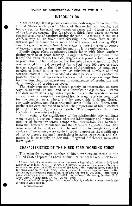
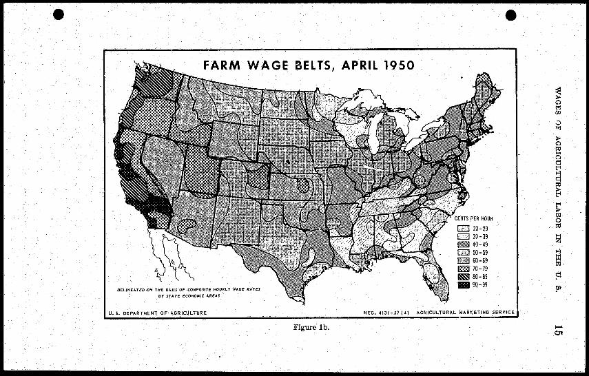
bull bull
~ ~
FAiR M WAGE BELTS SEPT-OCT 1954 8
~ ~ t til
~ lj
~ -
~ m t) t1 dD 30-39
_ 40-49
Qill]J 50 - 59 o ~mE 60-69
m 70-79 o gt ~ 80-89 ~ _ 90-99
C _100amp overDEljNEATED ON THE BASIS OF COMPOSITE HOURLY WACE RATEJ
SY STATE ECONO~IC AREAS ~ d ~
U s OEPARTMENT OF AGRICU~TURE tzlNEG lt132-57 11 AGRICULTURA~ MARKETING SERVICE
Figure le
WAGES OF AGRICULTURAL LABOR IN THE U s 17
Ohanges in wage rates in 110nfurm occupntiollS of comparable shill and status also should he considered in evaluating the increase
bull in agricultural nlge rates
FARM WAGE RATES AND FACTORS OF LABOR DEMAND AND SUPPLY
The Concept of Economic Regions
In 1950 the entire lnnd area of the United States was subdivided into homogeneous statisticnl areas called State economic areas It This was accomplished by grouping eounties hnxing simHar economic and demographic cbantcteristics Donald J Bogue and Oalvin L Beale later developed a second broader subdivision of economic subregions b~ combining simiJal State economie areas In 1954 two additional and cyon broader delimitations termed rieconomic regions and Ileconomic pro~illccs were introduced Eeonomic regions are combinations of economic subregions filld e(onomic provinces are combinations of economie regions These fOlll delimitations form a single integrated system of area e1nssiflCation which introduces the enyironmental or (cological c)]l1poncnt into socinl and economic studies Bogue did not inttnd to substitute this system of economic areas for other ecologicul areas but rather considercd it a necessary base upon whieh ecologieul ureas lllUY br plotted in order to discover more about ecologieul structure J
Fnlike Rtute economiC arcus nnd e(oJlomie subregioJls (conomic regions and economic proyineCs do not 1ue ofIicial status as units of area for reporting eeusus and othCr stntislics collected by the Goyernshyment Bul for the purpOSt of the prCsCnt study economic regions provide a highly useful busis for hu ncUiJlg a large mass of wage and related dula (fig 2) In the anaIysis of farm wage rate differentials and r(nJ(d lIl(llStlrCS of labor demlnd und suppl~~ that follows the economic region as a unit of area is used
The composite hourly farm -age liLhs hy economic regions for 1950 and 1954 arc shown j)1 table 7 The complete list of related factors us(d in the analysis iF giyen in table S
By grouping datIL from State reonomic arClIs into the 13 economic regions the geogrnphic vurintioll of fnrm wnge rates was compared with vuriations of 16 sp(cific itCUlS through unalysis of covarianceJ6
Thus the nssoeiation of farm Wl1gc mttS with eaell of the fact01s and their regiollal YlIriatioJls W(ImiddotC rnensuredby holding constantll
i4 BOGUE DO~ALD J A~D BEALE CALYI~ L ~CO~O~lIC sUnHEGIOltlS OF THE UNITED STNllS Series C(llsus~BAE Ko Hl 47 pp 1953
15 BOGUE DONAID JlN OUlJINE OF THE COMPLETE SYSTEM OF ECONOMIC AREAS Anl(r Tour Soe 40 laG-I 1954 Page 13G
Ie The region means of the cOlllposite wage ralei for the ltate economic arels were used in making the annlyses of covariancc ruther than the regional composite rates computed from ungrouped duta (method dCRcribed in Appendix B) The dilference$ betwc(n thc region lllcanR ill table 13 computed from the data grouped by State economic arca~ and the rcgional composite ratcs in tble 7 cl1l1pnted from the ungroupcd dutu ranged frolll 0 to 3 cents pcr hour
bull
00
COMPOSITE HOURLY FARM WAGE RATES ~ By Economic Regions 1950 ~
()gtshyt td
~ XI trj
ZRotlly Mllunhnn ltInd
IntelmQlIl1l1ln
-r -I
~ fJl t tl
~ o 1Unlhd Statu
vntoQe ~ 51lt o
sect
SOURC( poundtof1llIf ItrlDIJ n delineated by Donald J DOllie All Outline III Iht Co~pltlt Sysle~ 01 tonollilt Altu The Jmelican )ollrnaJ o Sotlc~ampL Vol lX No1 SfPttlllbtl 19t4 p m ~
l lZJu Dtr~flll(tjT OF CHICUllUItf tiED U-l1 el AGItCULTURAl 1oIi unIHG SpoundRVICpound
Figure 2
bull bull
19 WAGES OF AGRICULTURAL LABOR LIi THE U s
TABLE 7-Composite hourly cash farm wage rates by 13 economic regions United States 1950 and 195
bull Composite hourly wage rate
Economic regions
April ISep-Oct 1950 1J54
---------------------------~
--_----- ---~---------------~-----~---
I Atlantic Tetropolitall Belt_____ _ ________ Cenl
60 Cenls
84 II III IV V YI VII VIII
Eastern Great Lnkes and Xorthea~tern Upland __Loer Great Lnkes___ __ _________ bull _____ _ Upper Great Lakes_____ ________ _ North Center (COlll Belt) ______ __ Central PIllillS _________ _________ _ Central and Eastern Upland_________ Southeast Coastal Plain______________ _
53 57 43 52 61 I 41 33
88 84 75 81 87 61 49
IX Atlantic Flatwoods and Gulf Coast_____ _ 48 64 X South Center and Soulhwet Plains__ __ _shy 41 60 XI XII
Rocky lIfountain and Intermountain ___ Pacific Korth Iyet __ bull ____ ________ _
_ 62 82
78 108
XIII Pacific Sou th-ecL _ _ _
Fnited ftlte~ __
84
()shy-) I 100
79
Data published in the 1 J50 and 1 J5middot CenIl~e of Agrieul tUJe were baic to thelte computation made by the Agricultural ~faJkeling RClyire
geographic location find each of the 16 selected items ill turn hile the association betwcen fiL1ll1 wfige rates fiml one of the others was jnshywstigatcd17
Factors Selected for Analysis With Composite Farm Wage Rates
Like all socio-economic plHJ1omenfi the levd of farm wage rates is a result of many ecollomic demographic and social forcts The 1950 Census of Population find Census of Agrjcllli urc provicltd opportunity to il1Yestigate the fissociation of farm wage rates and otber items report(d for Atate economic areaR Factors selccmiddotted W(1( (1) )Jeasures of fnnll labor supply sueh as mtes of net ou t-migmtioll from the farm population extollt of ofl-ffLlm work by farm opcmtors and ext(l1t of Jlollfarm work by the rUlal-ffilm populntiol1 (2) measures of the demand for farm labor sueh as (eonomie sjze of til( farm (llteIshyprise extent of us~ of tmetols and ratio of larg(-s(fi]( farms to all farms flnd (3) indications of farml1rodultli~ity find farmls ability to pny as mens11l(d hy fnrm-op(mtol family J((l-of-living inci(x(s
17 The method of analysis followed is cle~clibcd by lL-Goou L-RGARET JARshyMAN AND Pmcgt DO STNlrSTICS FOR socrOIoGISrs 575 pp 1952 Chapter 24 For another application to analysis of demographic data see 13 OGUE D ONIfD r AND HARRIS DOHOTIlY JJ co~rpARATIVE POpUIrroN AND UHBAN HESIMHCH IA lIULTIPI~E R1GR1~SSION ANIl COVARfoINCl ANAInus Scripps Poundation Studies in Population Distribution No8 75 PPJ iIlus Miami Uniersity Oxford Ohio 1l54
bull
20 TECHNICAL BULLETIN 1177 U S DEPT OF AGRICULTURE
TABLE S-Correlalion coefficients oj composite cashjarm Uage rate] with selected jactols 1m 361 State economic areas 1950 1
Correlation IFactors dth com- Significance posite farm I CF) bullwage rates
I--Farm labor supply
X
X3
Xl
Xs
XI
Rate of net ollt-migration from the total ruralshyfarm population 1940-50_________________
Rate of net out-migmiion from the 1940 rumlshyfarm populaUon aged 15-19 1940-50_______
Percent of rural-farm population employed in nonagricllitural indusiriei 1950 ___________
Percent of farm operators reporting 100 or more days off-farm work in 194L __________
Replacement ratio for rural-farm men in workshying age grollp 25-139 1950-(i0 ______________
-408
-395
1138
262
- middot~70
I 71 5
66 2
104
265
1Ol 6or
Farm labor demand
X6
X Xs
Average llluc of land and bllildil1ggti per flrm1950___________________________________
Percent of farms reportil1g tractors 1950 ______ Percent comnl(rrial farms comprised of allfarms 1950_____________________________
576
487
117
l81or 111 9
5 oor Xv
X IO Xu X I2 XI3
Percent Economic CluRs I lind II farms COIllshyprised of all farllls 1950 __________________
Average value of products sold per farm 1950_ Average size of farm in acres ]J50 ___________ Average value of livestock per farm 1950 _____ Percent livestock and livestock products are of
all products sold 1950 ______ ______________
5213
545
245
226
113
137 1 151 6
22 8 193
46
Level of living of farm operators families
XH
XIS
X I8
Farm-operator family leel-of-li ving index1940___________________________________
Farm-operator family level-of-living index1950___________________________________
Percentage change in farm-operator familylevel-of-living indexes 1940-50 ____________
670
657
-577
291 8
273 0
1793
1 See Appendix C for definitions and explanations of these factors Significant at the 001 leveL Significant at the 01 level Significant at the 05 len
Comparisons of Differentials in Farm Wage Rates and Measures of Labor Demand and Supply
In developing the analysis of covariance the total association between farm wage rates and the factors of labor demand and supply were first considered for the country as a whole without regard to regional classification
The relationship of each socio-economic factor to cash farm wages and wage levels was estimated through correlation analysis and
bull
WAGES OF AGRICULTURAL LABOR IN THE U s 21
particularly 1nalysis of covariance in which the effects of regional variations could be analyzed
bull Because factors of fUTlll labor demand and supply are not distributed
symmetrically over the country one would expltct simple correlations of composite cash farm wilge mtes and anyone of the factors to give relatively low correlation coefficients The results of simple conelashytion analysis shown in table 8 indicate this to be the cuse When the values of each factor are correlated with composite hourly farm wage rates for the (ountIT as a whole the resulting rs range from 113 to 670 All of these 18 are however significant at the 05 level
Wage Rates and Labor Supply
It is not surprising [haL the 1950-60 average Lnited States replaceshyment ratio for rural-farm men aged 25 Lo 69 was one of the supply factors most strongly associated with the levd of farm wages Farm wages tend to be lower ill areas where thp supply of men reaching working agp is larger than the number leaving this age group Of more directly is larger than the number needed to mpet local farm labor requirements The long-term downward trend in farm labor requireshyments and the relatively high birth rates in some rural areas particushylarly those areas of low fnrm income in which the absorption of thA available labor supply hns been least successful have worked to keep farm wages depressed and to intensify the problem of rural undershyemployment The pull of more attractive labor markets was reflected in mtes of net migration from the rural-farm population which ashypeared to have a strong association with the leyel of farm wages In this case the relationship was negative high rates of out-migration being associated with 10 farm wage rates
On the other hand composite hourly cush farm wage mtes appeared to have relativlly low correlaticn with thc proportion of ruml-farm population employed in nonagricultural industri(s for the country as a whole or the proportion of farm operators reporting 100 or more days of off-farm work in 1949 rrhese correlation coffieients are cornputed from the 361 State economic areas without taking into aCCOllnt regional classifications As is shown in the discussion which follows these factors were quite strongly associated with farm wage levels in some economic regions h(1e altellll1tiTe employmcnt opporshytunities exist in abundfillcc find in otbers where fl seriOliS degree of underemployment exists among the rUJfil-farm populi1tion However the relatively low total nssoeiations shown in tabl 8 indieate that there were more regions in which these fuctors ere not significantly related to the level of fnlm mgts
Wage Rates and Labor Demand
Factors assoeiuted with the demand for farm labor which reflect the economic size of tIl( farm oprration and the farmers ability to pay uppearccI to have the stlonglst associations with the lewl of farm wage Tates There were high cOlTrIations between the comshyposite wage rate unci tlw average value of lund und buildings pel farm the proportion of Economic Class I and II farms the proporshy
bull tion of farms reporting ttu(tors in 1950 and aV(lflge vn]ue of produets 44i139-58--4
22 TECHNICAL BULLElLN 11 77 U S DEPT OF AGRICULTURE
sold per farm On the other hand commercial farms as a proportion of all farms and avemge size of farm huel low correlations with the composite wage rate COll1lllercial farms 18 as a proportion of total farms varied compartttively little between [ueas (table 12) Further- bull more since commercial faJms comprised an average of about 70 percent of all fan1ls in the United States and hired 925 percent of total hired workers in 1950 and 958 percent of all hired workers in 1954 the inclusiveness of the broad category of commercial farms obscmed possible variations among areas that might be associated with the level of farm wnge rates
Average size of farm on the other hand varied considerably tluoughout the country ranging from 88 acres in the Atlantic Metroshypolitnn Belt to 1332 acres in the Hocky )fonntain and Intermountain area (table 12) However the lelationship between size of farm in acres and the level of farm wages is not clear cut As indicated later the character of the farm enterprise and its economic scale in terms of value of products soM bear a closer relationship to changes in the level of farm wages than the exton t of acreage per farm
With the eflect of rcgional variation unaccounted for farm wage rates appeared to hae little association with the average value of livestock per farm or the percentage livestoek and livestoek products contributed to the value of t)roducts sold But total correlation fails to show the variation in eieglee of association between farm wage levels and the pereentage of livestock and livestock products sold Relatively high correlation coefficients were founel in some of the dairy farming regions and in at least one stock grazing region The complement of this variable would be the percentage of the value of production accounted for by crops This might be expected to show n low negative correlation with farm wage levels in 1950 Sinee the 1954 census was taken in the fall of the yeaT when higher harvest season wage Tates previtiled and more seasonal lOrkers were elllshyplo~Ted it may be conjectured that the corrdotion between percentage -alne of liTestock procluets and farm wogo levels was higher in the fan of 1954 than ill the spring of 1950
Wage Rates and Level-ot-Living Indexes
Farm wage rates Were stroIlgl~- associated with farm-operator family level-or-living indexes for botb 1940 and 1950 Farm wnges were highest in the areas where the level of living was comparatively high Between 1940 and 1950 the highest pereentage increases in the farm-operator family level-of-living indexes oceurred in areas where the index was relative1y low in ] 940 Thus there was a negative relationship between the composite wage rate and the pershycentage change in the level-of-li-ring indexes that is the 1940-50 pereentage changes ill the level-of-living indexes were highest in areas where wages were lowest in 1940
18 Commercial farms include all farms with a value of farm products sold of at least $250 except that farms with a value of production as low as $250 to $1199 are defined as commercial farms only provided the farm opemtor worked off tile farm less than 100 days or provided the income the farm opemtor and members of his familv received from nonfarm sources was less than the value of all farm products soid bull
WAGES OF AGRICULTURAL LABOR IN THE U s 23
Interde~endence of Wage Rates and Other Factors
bull The techniques of partial and multiple correlation brought out
some interesting findings on the association between farm wage rates and factors of labor demand and supply Of the selected items which have been assumed to represent various aspects of the demand for farm labor X 6 average value of land and buildings per farm showed the highest simple correlation with farm wage mtes + 576 It was alEo noted as was to be expected that X6 was highly correshylated with the other factors of labor demand from +588 (percent of farms reporting tractors) to +906 (average value of products sold per farm) Item 6 therefore was selected as an indicator of labor demand for partial and multiple correbtion analysis with farm wage rates and factors of labor supply
On the labor supply side X 17 replacement Tn tio for working age group 25-69 1950-60 had the highest zero-order correlation with farm wage 18 tes - 470 The correlation between X 4 percen t of rural-farm population employed in nonagricultural industries and X s percent of farm operators reporting 100 or more days of work off the farm was +924 Therefore X5 (which had a somewhat higher corshyrelation ith wage rates than X 4) was used to represent the~element of alternative employment opportunities The replacement ratio X 17 was used as a measure of popula tion pressure on the lanel or unshyderemplorment
The representative items of labor demand and supply are X6 factors related to demand for farm labor Xs measure of alternative employment opportunites (supply) Xl population pressme or underemployment (supply) Xl composite hourly wage rate The simple partial and multiple correlation coefficients Wele as
follows 116=+576 1165=+686 r165 (17) = + 688 rla(i)=+604
rI5=+2G2 1156=+513 rIS6(1)= + 439 r15(li)=+163
r1(li)5=-431 11 (Ii) 56= - 437rl(li)6=-510 R156=+713
R I5(ln = + 492 R16(li)= +711
RI56l17)=+middot775
The demand for farm labor as represented by X 6) appears to bear closer association to wage rates than either factor of labor supply The correlation between wage rates and labor demand is improved only slightly when the effects of either factor of labor supply are allowed for On the other hand the correlation between wage rates and off-farm work or underemployment is substantially increased wben the effects of labor demand (X6) are accounted for Moreover allowing for the average effect of X 17 decreases the association between
bull wages and factor X s the extent of alternative employment opporshy
24 TECHNICAL BULLETIN 1177 U S DEPT OF AGRICULTURE
tunities Some of the apparent association between wage mtes and alternative employment opportunities is accounted for by the relushytionship between underemployment and the extent of alternative employment opportunities The relatively greater effect of labor demand on wage rates is also apparent in the multiple correlation coefficients The Rs obtained using X 6 the labor demand factor and either factor of labor supply Xs or X 17 are greater than the R obtained using only factors of labor supply (Rl5(I7) Apparently average value of land and buildings per farm is a strong indicator of farm labor demand As noted before average capitalization per farm was highly correlated with other elements of farm labor demand 110reover all factors of labor demand investigated were rather highly intercorrelated except X 13 percent li--estock and livestock products are of all products sold
On the other hand the selected factors of farm labor supply were not strongly correlated with each other except for X 4 and X5 as noted earlier Since changes in the supply of labor are closely linked to a broad range of socio-economic factors and personal motivations the selected factors of farm labor snpply are likely to be more diverse than those of labor demand in which the economic element is predominant This could be merely a result of the limitations of the items available from the census which have been assumed to represent elements of labor demand It is more likely as indicated earlier that the factors which influence the supply of farm labor are far more complex and diverse than those influencing the demand for farm labor
Such speculation can easily be pushed too far Only 60 percent of the area variations in cash wage rates are explained by the variables of labor demand and supply used (R2=60) Higher order correlations would of course increase the amount of variation accounted for by the factors employed but with a lessening of reliability19
It sbould be remembered that tbe correlation coefficients developed in the foregoing analysis are total correlations in the sense that they do not take into accolmt regional variations in wage rates 01 labor demand and supply Regional aspects of the association of wage rates and the selected factors ill next be evaluated thlOugh the techniques of analysis of covariance
The Regional Effect
The 1950 average composite hourly wage rates for the 13 economic regions shown in table 7 runge from 33 cents to 84 cents Analysis of variance shows that the regional difJerentials are sip-niiicant that is the chances are better than 999 in 1000 that the regional difrercnces are not dne to chance fluctuations Similarly the regional variations in the other factors under investigation were found to be significant (column 2 table 9)
The total correlations between farm wage rates and each of the variables were found to be significant and composite farm wage rates as well as each of the selected variables showed strong regional clillershyences We now wish to discover whether the association between composite wage rates and each of the other variables for the individual
10 SNEDECOR GEORGEW STATISTICAL UETHODS Iowa State Oollege Press Fifth Edition 534 pp 1956 Pp434-435
bull
bull
bull TABLE 9-Analysis of Variance and coVariance composite howly cash farm wage rates selectedjactols and economic
leaions 1950
bull Sigllifiennce of the Signiflcltnco of tho
Significance of LSBOshy Signifilnllce of c1iffershy pltltial Itssociation plllLinl associntion ciation brtlloell Signilkanee of as~ushy ellee between iushy IJetlleeIl composite between composite composite hourly ciation of cOlllposiLe (lhirhml region reshy hourly Vngo mtes hOllrly wngo mtos J
Selected factors wage rate lwei hOllrly wage rates gressions of COIUshy and regionnl vaJiashy nllci oneh of tho gt oarh of the 0 ther and caeh of the posite hourly wage Lion hen renional o thor selce Lod facshy G)
lltjselected radors for othcr sclett~d fallshy raLes 011 elwh of dirrNences iJ7 eael tors wholl vnrinshy Ul 301 State ecoshy tors wi til rcgiolllLl the other selected of the other selected Liolls ill regionltl onomic areas classifjra Lion factors factors have been lo(nLion lLrc alshy IJ
allowed for lowed for
i gt
(F) (If) (F) (F) (J~) G)
1__________________________________ G50 ]5~1-----shy2_______________ 715 23 J7 J 8J 52 7 3_______________ O~ 2 21 52 2 00 50 2 (I)4_______________ 104 38030 1(i 2 02 72 3 ~ 5_______________ 2~ 5 2fJ 15 1 I 37 G5 3 27 36_______________ 178 1 tlt31 Otl 5 737_______________ 1119 70 70 2 07 Ed8_______________ 50 23 73 L 88 64 3 127 o9_______________ 1371 d2500 4 1410______________ 151 0 R 37 5 1511______________ 8 2l2~ 2871 008 12______________ 193 2404 1 88]3______________ 46 27 78 5 07]4______________ 2018 7middot1 13 442 ~ 15______________ 273 0 G5 II 432 ~16______________ 1703 35 30 a 7517______________ 1016 1307 3 OJ J
gt- __--_-----__---- shy~------
I Not significant Lt the 05 IOle
Signifiean t at the 001 lcvc Significan t at the 01 level IV Significant at the 05 level Cl1 For identification of fctors sec Lable S
26 TECE]HCAL BULLETIN 1177 J U S DEPT OF AGRICULTURE
economic regions are suHiciently similnl that We Ciln ilSsume that the chnraeieI oJ the rdulionships do not (lil1(r signiLicflnily from one region to flllother Column3 of lablt 9 indicntes thM til( aYeInge r(latiollship (lill( of ngllssion) b(t(gt(11 fnnn wage rates nn(l most of tIl( other yariablps dif)e1ed id(ly among tht rpgiom For tlJ(se variables an assumption oJ uniformity of 1(gionnl rplalionsbip with bullwagp ralpfl apP(lllS to be UlllJTlu)lpd Although 0)( correlation bel((ll wng(~ nttts and such Yllriabl(s (for Exunplc ny(mgt yalup of land und buildings or fiY(lllglt alup of products sold) Wtts l(llltiyply higb tbe tlSt mndt in column 3 of tnblt ninciicatplt thnt til(gt (LalucL(l of the associntioJl within ngions (us lCprPfHllpd by the slope of tbe liup of l(grltssion) ciifrp(d to n grpatpr px[pnt thnn (ould b( nttlibutp(l to (hnnce As ( shall spp Int(r in thf ciiflCllssion of the nssocintiol1 bet(en wage mtefl llnd tbp Ynli(tbks of Jnbol dpmnlld (tnd supply ithin thp s(pnntt( ngions tllP ldfLtiorl~hip may cbange from positip to l1(gntivp fOm Oll( l(gioll to tb( Jl(Xt For lxample higbpl ffirm wages WP associn(pd ith higIHl nnmg( [arm sales in tb( Atlantic IIltropolitnn Bdt h(l(ns highpr farm nglS were fissoein(d ith lowpl nV(lagp fnrm sulls in the l-pppr Grpnt Luk(s rpgioll For lbpse relationships inpstigntiol1 nt tll( ](giOlHlllpvpl would apPpfil to be morp fruitful thnn [ultil(l stud of LIt onr-tlll nss()(jntions
The J)Pxt st(P in n lllllyzing (hp l(lHtiollship bel (en farlll WIIglS find the spl(p[(d ynrinblps of labor dp])HUld und supply is to dlt(rmine hltlwl (hl g(ogrnphic dilll(lltin]s in fnlll1 wag( rnlps can 1)( a(shy((lun(pd for by t hl lgionul difilPIHlS in th otlHl vlriablps Hoshy(Vpr sitJ(p thl stutisticnl pIo(PciuIP for (sting this possibility (annlsis of (oYllrinnc) il1Yolls nn u$sUmptioll of uniformity in tbt rpgiounl nlu t iOllship Iwt ((11 tJw vilrin hIps in ltIll(s ion tIl( test canllol be made for thosp fttelols whidl sho highly significlLllt diflprll)C(S among th(ir lPgimnllllntiollsbips itl fllrm Wlg lnt(~ But s(llnl of the 1ltrIPSSiOllS tpflted in (olumn l of tltbJp l st 0 ((1 Rufliei(ntl slightr diflCl(ncps bpt((11 l(giolls to mnkp thl nntllysis of (OVtlrifll1(0 fcasible Thp J1ntulP of tlH tlSSOcilltioll lIS illdicn t(el bl thl illdiYiclunl 1(gion JEgllssiollS 1)(( (Pll (om posi t wngp nl tps i111d ofr-farm work hy flllm optliltOlS 05) shOld no SiglliHcu II t diflprPJl((s 1)(1 ((11 l(~ions thp l(giono 1 llgIPSSiOHS of wag( Ill t(s with llonfu Im (m ploYll1lnt (X4)
net migIn tiOlI of tillt lurnl-fnrlll population (X Hilt X 3 ) nnd proportion of comnHrciul Jnrl11s (X8) shOpd llgioJlal difi(rcIl((S si~llifiennt onl at thp 051cwL ith l(S])(ct to thpse iYltYnlinb1ts thPll 111l regional daflsifiCtlion dews lot neld mn tpriaU to our ability to prpdict ICY(s of farm wuglts Xote tltnt four of thpsc ynrinblps nrt Jl1PllSUlPS of fnrm labor supplT
Column 4 of tn bl( 9 shos thp leslll ts of Ill( analTsis of eovnrin nee for tht fin YtlinbIs biet showed the most uniformIty of relationship with wagp nltes Obs(1Yl that tIl( vnrian(e in form wages (column 1) is leclu(((l aft(l nllowtll1(( is ma(iP Jar lPgional diflelcl1c(S in migrntion from the Illlal-furm population (X2 and X 3) but larger 11ftlJ adjustshyment foJ lPgionul difflIPJ1ces in l1onfnrml1nd off-farm employment (~ and X 5)aud [01 I)(r((ntage of commelcial farms (Xs) Yet reshygionnl difreleJlCtsLll fnrm mgps [emlLin highly significnn t llftPl regional diflerellcPs in ellch of tbrsp fndors p1e takell in to n(Poun t Regional diflerences in no one of t11psp fiYe pound[1((01S C1Jl wholly account for the regional Y1ri1lions in farm wage mtes
bull
WAGES OF AGRICULTURAL LABOR IN THE U s 27
Ye may now turn the question around and ask Is there a significant association between farm wage rates and any of these frye fadoTs
bull after regional yariations huyc been Temoyed statistically That is to ask if there is a significant average association between farm wages and any of these factors without Jegald to region differences Column 5 of table 9 indicates no significant within-region association between farm wage levels and net 0c~-nigrntioll of rlllal-farm youth (Xa) or p(gtrccnt nf commercial farIlli (Xs) But toUd 1l(gtt migration from the rural-farm population A2) and nonfarm and off-farm (gtmshyployment (X4 and Xs) each showd signifiean t al though low (orrelation with the lenl of farm wage la es after lemoyal of l(gtgionaJ variance (see table 10)
TABLE 10-Corrr[ation and r-cglcssiult C((jficifnts for composite hourly C(slt farm U)age 7atcs and selected facto1s 1950
I -------- ----shyi Toml corre- bull Total re- Yithin- Betw(cu-
Factors laUon I grcsjon region region (orrela tion correlation
(Xi) Ir) (b) (r) (r)
2 ____ _ -408 -528
-204- i -5793 ____ -31l5 -488 -0040 -72440- ___ lG8 l middot 157 317 1 0755 ___ _ 262 323 270 I 265 6 ___ ~~ __ 576 314 ]33 I 8377 _______ _ - 487 f 282 218 I 6038___ I
)-shy117 088 -088 j bull _Ii)9 --- - i _____ ~_ 52G I ]23 i 840t middot GSG10 ___ 545 401 m)7 830lL ____ -
~ - i 245 303 -ll7 I 540912 ___ I C)-r)22G bull _i)_ -200 55013 ___ 113 i 068 -015 i 20514 ___ (j70 I 74G 421 I 77415 ___ I I G57 70G 371 78516 ___ I -577 -340 -315 -74G11- __ I- - -470 I -544 -370 -615
I For identification of factor) see table 8 oI
For the latt(t thrN variables particuJarlr ~ and X s regional location has 11 lelativ(gtlyminor influence on their degree of association -ith fann wage rates TJlUs aspects of farm labor supply im-oh-ing aI temativc employment opportunj ties me seen to haye a universal efIect on farm wage rates although as Ducoff and more recently middotWeatherford have pointed out alternative opportunities have a much greater effect OIl labor supply and farm wage rates in highly indusshytrialized areas ~O
In the case of the remaining factor of labor supply (Xd the moyeshyment of wage rates seems to be eyen more sensitive to the pressure of surplus farm labor in regions which have great industrial centerfl (table 12) The relationship of rural underemployment to farm wagus
20 DUCOFF LOUIS J ibid page 61 VVEATHERFORD rILLIS D JR GEOGRAPHIC DIFFERENTIALS IN AGRICULTURAL WAGES IN THE UNIT~D STATES 99 pp illus
bull Harvard University Press 1956 Page 84
28 TECHNICAL BULLETIN 11 7i U S DEPT OF AGRICULTURE
also is nlrccted bc regionnl conditions on the lahor dell1nnd side If the seasonal demand for (nrm labor is heftYmiddot variutions in the ]eel of underemployment wiU be uecompanied h~- market variations in age rates rrhat is the slope oJ the ]pgrlsiion of wnge rlltes on replacement ratios will be stetp as is inclicatNl ill E(on01~lic Regions I III IV IX and XIiI for fttetor Xli in table 12 _Ul of tlllse rpgions bull are hea users of seasonal form labor and all of them dtpend on llllgratofY- -orkers during a part of the growing SN1SOIl
In the association I)(tween farm wnge ratts and llndpl(mploYllltnt as -ell as each of the otlWl sclectpd YaTiahl(s lPgionaIlocrrtion strongly influences eith(r the degr(e of assoriatioll (corrdation) or the churlwshyter of the relationsbip (line of r(grcssion) Or both (tnhh 10) Thpse relationships nre nil(et(d h- the lqionnl diilcrcnces in the economic institutions upon hich the farm cntprprisc is hased and till physicUl emironment in whieh it (xists
A closer look at farm wage milS lllld factors of labol d(llland and suppl- -ithin the 13 economic regions -ill pro--ilt( further insis-ht into the undcd)-ing causCs of Tllliotions in Jurm ugP rutes
Regional Comparisons
TIllsou(hC[lsl(lll pnrt of tll Lllilpd SlallB (EcoJlomic Hegiolls VII -III IX nud X) is gltIHrnlh- ehuluc(priz(d hy 0I1P-Cl0P farming opllztiiOlIS lypifipd by (olton OJ lobneeo fnrmsLuek of diYllificHshylion impurts n rigidity to tllP farm llllP1lgtrisl thut irHr(llS(S the Illumrds of ((ollol1li( fluctuations ChnrnetltJlstics of tllt soil and terrain and thp (xisi([l(p of ullltiljll1ploymtJlt nmollg til( Jurnl-Jnrm population haVi 510(d ll)[(hnnizatiol1 of lUlm Pl(HltHt ion CYIIl wllll1 this is possibl Lnrgl quulltillPS of lllbor nrp twnilnhk through shancropp(t und othll ttlllll1i furming nlntllglIIHllts which glIlPrally illcludp 11lt use of lnrgp 111lll1J)(]S of ullpnid fUllil- work]s jltlrnflshylive nup1oYlll(llt OPPOllUllilils whilt lll(j(nsiug 11( still nlatinlshyselllTP in thp South ligrnlion from til( furnl-furm population ill ill(gt South lll~ hlPll lelutiw1y high ior tIlt lolld mrnl-fulDl pop1l1ntion tl-o pH n for farm ~-outlt- ((killf [hlir iit full-lime johs TIlt rnio of llumlwr- lt)f llWI1 ll[pJing llw Olking ltg group to those leadng it (1( [110 lligh (ompnrpd to oilpr part of Iht cOUlltry TIl( gllIltlul pietlll( i- OIH of l(intiy(ly 10- ]pnIs of Ih-ing amI 10
farm yugP rnlp low proportions of nOllugieultund lHlploYlllenl and small farms with low (npilal innstmPllt (omptlrlltinly fpJiTCsock and rllati(ly 10- yull(s of fnlIll production (fig 3 and tablp l~)
In such ciJ(u1l1slnl1((s it is not surprising to filld tlml the Statr eCollomilt areas haying tIl( highrst 11lt migration or lPplnc(lllClJt mtios among th( rund-ftlrIll population 21 oHell han th( lowest wa~e ntt(s 1lgion VB the Crntml nnd EasteJu Fpland was the onl low-wage ngion w1lpr( lhcn~ was 110 significant jdationship bttTP(1l the levd of wages and the magnitudc of thtse popuIiLtion Chnnges This region just north of (1( onc-crop ar(a is eluUuctCJiz(cl by general fl1rming und out-migration is somewhat 10(1 timn in the regions farther south HowPycr ill lpgiol1 VII as -eli us legions VIII and IX there wus it signifieunt asSOcitLtion between the level
1 For an explanation of the mjgmtioll and replacement mtios see Appendix C
bull
bull bull DEVIATIONS OF ECONOMIC REGIONS FROM UNITED STATES AVERAGE IN COMPOSITE HOURLY WAGE RATES AND SELECTED FACTORS19S0
IX) x I IX) RATe OF NET MiGijA nOr fRaIl 1940-50 IIET MIGRATION OF RURAL
COMPOSITE HOURLY FARM -1GE RATE RURAL-fARM rOPULAnQ~ 1940-0 FARM POPULATIOII 15-19 IN 1940 ~1---shy trI rn z
I~ 0 1 g~
9 _ 10
I ~10
ltgt
I I r o
11 13
1
~L_if -10 -10 10 10 middot30 -10 -10 0 ltl -10 10 +10 +20
CEtUS PERtUIT PERCEtiT (X) x 1 (X)
PERCENT FARM OPERATORS REPORTING ECONOMIC CLASS 1ANO n FAR~S AS REPLACEMENT RATIO FOR 100 OR MORE DAYS OFF-FAR~ WORK 111949 A PERCENT OF ALL FARMS 1950 WORKIIIG AGE MALES 25-69 1950-60
== I ~011 I I Z 53 3 o
I tu ltgt 5 I I
S 5 6 6~ 6
u 1 a 2l t a o 9 l 95 5 I8 10 10 10 10
W 1 II II UIl 11 11 13
1
tamp ~ ~ _~ __ ___~~1 II ~ -n middot10middot 10 10 -10 middot10 10 10 -80 -lO t30 t60 -so -30 +30 HO PERCENT PERCEHT ItiDEX RATle rER 100 2
IIfCAUf 0 OFER~NcfS IN lCAt[ tfHCTH OF 8411$ ARC HOT INDICATlVC or RELATIVe eNlrVDE OF OEVfA TIOHS IN RffPECTlYE ACTORS
v s DErA~TUEHT OF AGRICULTURE ~EG bull bull 1)0-11 I) 4CRICUlTUQL luRkETING SERJICE
t)Figure 3 ~
30 TECHNICAL BULLETIN 1177 U S DEPT OF AGRICULTURE
of farm wages and the prevalence of nonagricultural employment and off-farm work Where alternative employment opportunities did ex--ist in these regions farm wages tended to be higher
In Region VIII the SoutheasL Coastal Plain covering paris of bull Virginia the Carolinas Georgia Alabama Mississippi and Tennessee the factors reflecting demand for farm labor appearCd to have little significance middotwith regard to the lCvel of wag(fL ThC]C was some tenshydency for wages to be 10wC1 in State economic- areas where the percentage of (omn10rrial farms wos ltiglHr illid where the anrage size of farms was brger
For example in tlle StatC C(onomic ar(as of southCaslClJl Alabama and southCstrrJ) G(orgin farm yug(s w(r( below the Imiddotpgionnl an-mg( and farm ucr(llgCs and pPJ(pnt of (omn1Preial fanns C1( nbovp 11p rCgional a pmge iu 1950 On tll( ot11(r hand Stn [p p(onomie arpns in t11p [xlile arpas of tIlP (nrolinnshlld ldntiply hi2h fnrm wngCs small fnlms amI low pple(n (nglts of (ol11ll)prc-ial farms 11 [11( AJnlHllnuOporgin Sta( ((onomic ar([IS lllPn[iOIlNI tJl(J is an almost eompl(tC Jnek of nlt(ruatin Pl11plo)uWJlt opportunitips wh(rC)s tl1( (nrolirHL IlT(ns )n ill tl1( h(art of tllp souUI(rn t(xlilp district ill whi(h tlw proportion of tllf rurnl-fnrm populltioll lmployrd ill nonfarm work is grrat(l (hnll thl pJOporlion pmployed ill ngriculturp In H(gion YII wngps t( nc1pd (0 1)( highpl 11(j( t11(1( mrp more Economic Class I n nd II farms and h(l( th( proporl ion of liv(stoek in toull fnnn snIps 1ms grpntpr but ngltin U1PS( nssocinlions WPlP Ilot hi~duy signiJiCal1t
Thp cllmand fHCtOJS nppNuNl to Iw 0111(h moJt important in d(i(rminillg 11( 1(n1 of farm waws ill Eeollomie HpgioJi X tl( South C(ntpr and Soutllw(st Plnins just w(st of the lissisippi (figs 2 lnt 3 )nd ttlblp ] 1) hut th(8( nppfumiddotPlltl- had no paJticulnJ b(tlring 011 thC lenl of fnrm wngp raIlS in Economic H(gioJl IX the Atlantic Flnt-oods nnd Gulf Consl Hgioll This l(giol1 hassolUlwlJnt diff(lClll ehnrnCi(ristics flom tlH J(st of l1H SOU t h It hn a (ollsicpJoblp nr(L of nonfnnn [(JJi(or in Floliltilt Ilnd SOJl1( g(llpnd farming nJNS but is (specially not((1 foJ fruil truck nnd spNmiddotializpc fanning (im]uding riel nnd sugar (liM) GplHmll)- tllp proportion of (0111shy
l1lltreitll fnnns is low in this J1giol1 but Ill n-(Jtlgl siz( of fnll1 is large (I1r vlll( of (ipitnl inYlstnwnt is Jlhltiyely high tJnd tllp nlue of products sold is high
In Eeonomie Rgion lV the middotUpper Great Lakes (tht lnJcs eut-ovlr fringe in l1orllwlll MiIlllcsOt n riseollsi nand lieilignll) cia iry farming is eombiJl(cl with g(J1P1nl farmillg or the raising of hny 01 pottJloes and the value of ]h-estolllt 1)r fnrm is highCr than avprnge Gl)Hrall)- farming is on a small scale Although tIll proportioJl of commprcini farms is r(lativ~ly large in this llgiol1 UI( percentngl of Eeonomic Class I and II falms is low the IWPJnge siz( of farms is smnJlcapital inv(stment aside from tractor ownership is low and UU value of prodshyucts sold is low A1nong the rurnl-farm population out-migration of the 15-19 age group was relatively high bptween 1940 and 1950 but total net migrntio1 betw(w)) 1940 and 1950 and the) 950-60 replaceshyment ratio for men aged 25-69 years were low Thple nre relatively few nonagricultural employment opportunities in this region and in general it is characterized by small-scllle owner-optrated fnrms on
bull
31 WAGES OF AGRICLLTURAL LABOR IN THE U s
wJuell hircmiddotd ffirm labor is imporllII [ only in thpound SOli [hem Il11rt w]WIC fnrmillf op(rntiOJ1S an mOl( (x[lllsin
bull nlls( CItarnetprilttics ill RCgio)) IY uSllallrplll ill fiJl innrsp rPinshy
tiollsitip hll (111 tILl hwl or fllJlI WllgltS nllltJ UH lumiddotious supply nnd dlmaJl(l factos Tl( frtl tPI lh( IpHl of JlPl ou tmigrat ion the hig1uI tiLl wugP rntl th( ~l(1lt(r tll( jJloportioJl of (onmwJeinl fnl111S the 10Wl tIl ng( rut( till higitPl tlip ynlul of plocluets sold tlll lower tll( wage rnlt tl)1(l so 011 111( higlHct [l(rngp hOlld~ wag( in Rqion IY in Hli)() wns ill ~idligl111 oE I tlH copJlPl (ountry Ht thC wpstshyln (]1(1 of ll1( llJlJl(l JwniJlsllln TIL( farms Ul this Unfl nrp )(lati(I~ small nlld tItpound plOportiolL of sllbsis(pl(P fnrms i~ )PJntiyply high Offshyfarm pmploynwllt OPJOllllllili(s lin 11S1Ill11~ p1ltllliful in mining nJHl lllml)(ling in dust Ii(s Tl)(lo-psl nPIug hourly wn~( rilles ill l(~i()H 1 in Hlj[) WPI( in t11( (()1 lml is(OllSill ill(US ill hidl dairying is the Ill(ciomiJlnll t III rill Pll t (Ij)list mttl nil (llll Iiv( PJllploynHJ1 t opporLushyJli li(s n1( (onlpnrat iy(l~ j(
The Enstln) C r([l t LnJws Ilnd orlll(nsf l ]llnl1(l (Ecollorni( R(fioJl II) nlso eompris( 1l1CgiOll Jlrjmnlil~ of dniry fnrming itll S0111( S]Wshyciulizpd nreHS S11 eli as t11( poln I (j growi IIg n(ttls in ~ rflint and fluit truck mid mixNl fnrming 011 the S()lltlHrn shol( of Jqkp Ontalio_ In thi rpgioll hOHY(l thCip is n Jnrg(r proportion of Economic CJass I nnll II fnnlls nll(lllatin llllplo)-l1Hllt opportuJlities an grlll[lJ nnd oul-miglnlJl und replnc(llwll( Ifitios for tilp rural-farm populntion arC llIat inl~ 10 oollle tplIcl(ll(~ for farm Wtlg(S to b( high is iJldiculpd in otnlp (conomie nl(ns wlu( ill( proportion of EcoJlomie Class I and II farms wts elltiYel high nnd n sllongp] IJI(llll(y for WUf(S to be low wh(J( the vahlC of IiYlstoek WflS hifh_ Xo signiiicnnt rdltiollship was fou1ld 1)((wc()1 Ihp lenl of fnrm wuglS illld clilLngps ill pOJmlntioll nonngricultural Plll])loYlllCllt or kni-of-liiJlg- illdlxls
Tn th( LOnr Greal Lnkes lCg-ion ltlnir fanning- is n(compnnied hy fruit truck fIJl(lmL(d farming plinltipnlh- OIl the (11SPJl shore of Lake Jicliignn Hcn ho(yp~middotth( propoilioll of (ommpleinl farms including Economie (In] und n farms is rplnllYlly low uIld fnrming ojwrntions arC c(gtmrull on a smull senlC Thp proportion of 1l01lshy
ugrinrli ural (JupiOnllllt nmOIlg- the lurnl-fulll1 popuJnlioJ] is higher tlwn ill uny olll(j ((oI101)i( llgion alHl Jlpj olli-miglnion of the rUIul-fulJI 1 populntioll [1S (OIl]HllutLYlly lo 1]1(1( -ns s0111( tPIHl(IHY for fllllJl wnges to hp 1lt)- in o(nt( ((oJloIli( nrpllS wllel e lwl Olll-JJ1igIHlioJ) of the youngr ruml-fUlJll popuintion -US lPintiYcly high (labI( lll But ugl 1((ls lt1( 1l0l( strongly nsso(intcd with tIll llljOmiddot(j() ]pplntlJ1lPIlI r1tio for JI(11 ng-(d 2i-iD bCillf lower ju UI(as II(I this llpliHCI1H1l1 rutio WtlS high
JiJOuglr high form wl1gps (11 nssocin t (lei with high (ll pi nl illYlsshyllHnl und YlIluf of ]lIollncl iOIl sf IOngltI posi hi nssoeiul iOIlS WPIC
found 1)(( W(PH (1 t (he (onposit( wngl ml( and [llrm operators family iPnl of liying nlle (2) t11( proportioll of 1i((0(1 find li(slo(k plodshyllCts in totnl ytiltH of jl1odu((ioll 111 flU of (il(HP dairy lpgions n highly Si~llij(nnt ttlJltl(IHY foJ fnrm wogCs (0 hC 10(1 wus indicatcd ill unns il(I( Iins(ok nnrl ]i(slock produ(ts (ol1stituted n high propOlliOIl of snIps Thus it nPPCtUS (hnt dnir- fl1lJllS ptt~- Jowlr lIgps hut dUll fllllllS oftln hirp work(rs hy tht ntonth at tt rail
bull whieh work out to n cOlllpnrntiyplr in houd) rutC though room fill(i hourd OJ hous( nnd 0(11(1 pltlquisics flle nddd The yalue of
~
I l5
TADLB l1-Signijicant correlations betwren compos1te hourly cash farm wage rate and selected factors 1950
Fnetorsns~oclated with Fllctors assoclntcd with the supplr or rarm blhor the demand ror rarm
tljlabor
Popuilltion chmgcq NonlIgrlculluTIII elll Extent or opermiddot COlllpo~ltc ployment atlons ~
honrlyEconom Ie regions wugc
TIlle Percentllgc Perccntlgc Percentage ~ lotllinet Agc~ 15middotlU I Rcplilcemiddot nongrlmiddot operators Econ IPercentage I-migration net mlgrn ment Tlltlo enlturnl w100+ CiBSS I rarms with I-tlon or men ngcd employmiddot dnys olTshy I [ rarms tractors 01
25-69 ment rlmn work ~01
Correlation coelficiwuCent ~ United Stntcs bullbullbull __ ~bull_bullbullbullbullbull 52
VIII Southenst Constal Plllln __ 35 -~ 500 _ ~~ ~ _ 584 492 _ __ ____ ___ _ Jl VII 43 __ __ bull bull ~g 4211 bull2Ill
X sect~~tfth~~~e~~rS~Yt~~~~tmiddotLiill 44 __ __ bullbull bullbull ~ bullbullbullbullbull ~ -424 _ 381 740 ~ IV Upper Oreul Lnkes bullbullbull__ ~ __bullbullbull__ ____ 44 740 700 - tlSO bull 855 bull SGtmiddot ___ -005- l L Atlantic Filltwoods ltd dnH COllsL _ 48 bullbullbull_ ~ bullbull __ -800 542 _ _ If Ellslern Grellt ]Ilkes nnd Northeast Uplnnd 53 __ bull ~ ~ ~_ HO ~ V North Cenler (Corn Belt) ____ 53 _bullbullbull __ 294
III Lower Oroot Lllkcs M _~_ ~ -452 -62 _ _ _ ~ 515- 686 o VI Centml Phlns 60 _ w _~ ~ _-lt __ ~ _~_ ~ ~_ - ~ _~ ~ _~~~~ ___ -yen __ gt1 __ ~
I Atlnntic Mctropolltan nelL 61 ~ _~ ~ -72nmiddotmiddot 50- ~ ~ 1))5 XI Hocky Monntaln and Intcrmollntllin ~ ~ tH -444 ____ ~ __ -450 44 gt xu Pllclnc Northll(middotst bull ____ ~ _~ ~ bullbull __ ~ 81 __ ~ ~ __ __
xur Pllcillc SOllthwcst ~ 81 -806 ~ __ _ _bullbull
Only stntistiCIIlly ~lgnlncanL corrclllUons lIf(l I~tcd -slgnlficnnt lit lhe 001 level -significant lit the 01 level -slgnillcllllt lit the 051evcl I bull bull
bull bull
TABLE ll-Significant correlations between composite hourly cash farm wage mte and selectecl factors 1950-Continued ~ o lj mFnctors BSSoclntcd with the demnnd for farm Inhor
Farmmiddotoperntor fumll level-ofmiddot o living Indexes l
Abllltymiddotlomiddotpay JImiddot~poundtockCompositeEconomic regions hourly
~ cwago Percontnge Avemge
rote commercial size of farms arm Vlne VIIIIIO Valne )crcon ttlge Percellt
land nnd products livestock livestock 1l4O IUSO chllnge buildings sold per fllrm Is of sales 1040-1050
Correolion coelicienlJOel1U United Statcs bull___bullbullbull 52
Vln Southcast Coastal Plllln __ 15 VII Centml BOd Eastern Upland 41 =~~~~ ~~=~~ ==1== l~i~i ~~~ ~~~ =~~~
tllX Soutb Center and Southwest Plnlns ____ bull 44 728 lJ(l(l 420 bull [() 55l 846 821l -700 oIV Upper Oreat Lukes___ bullbullbullbullbullbull 44 DC Atllwtlc Flutwoods Ilnd Gnlf Const 48 II Eastern Orent Lllkcs and N orthetlst Upland 53 ~~~ 1~~~~~ -~~I~~~~ ~~~~ ~=~~~ ~~ c V N ortb Ccnter (Corn Delt)__ ___ il ----- -- --_- - ~ ---- ~ 1- - - -_ ~ Z~ ~ ~~ ~
III Lower Orent Lnkes __ 54 __ _______ h8 551 _ bull71 GII 11l7 -011 VI Centrnl Plnlns (10 _ ___ ___ _ ____ 3i2- _ __ __ _ _ _ __ ~ ~ 56-1 5ramiddotmiddotmiddot _
I Atlantic MetropolltBII Dell 01 ___________ - itUmiddot 510middot n04middotmiddot _ _ ___ _ _ 810middot i45middot -001middotmiddotmiddot XI Rocky rfonntnln nnd Intermouutllln 04 ~ XII Pncillc Northwestbullbullbullbullbullbull___ 81
XUI Pacillc SouUmmiddotest_ __ 81 ~ ~~~~ ~~~I-~~- ~
Only statistically slgnlllcnnt correlations are listed middot-slgnlficullt at the 001 level -slgnIIlCIIllt at tbe 01 level -Slb111flCIIllt nt the 05 level l
~ ~
------
--
Co)TABLE 12-Regr(ssioll cnlttJicirnts oj (olnpo8poundlr hourly c(1sharln W(1C rate~ on sliertedJactrmjor 13 economic regions1 1950 ~
-E-RO-e~-li-~~l-liC-r ~2 I X3 XI XI X6 middotx ~R Xu i Xlo Xli X I2 T~l rI~-r~~~-r~-l-~- ~ ------_-~----J~I----2-I-s --81~i--l-U~5~-~~----1--8-~17i-1~~-5-J-n-5 5I()j -21(1----0-0-31--r-5-1
-shyL __________ _
1 ImiddotW - GnO - 1 Olfi ~ [L ~---r----ou~ 252---ilJ~2G2i--~55~()Ul-~2I(r~-5()-I---12r - 0771=1 middotJJl~-7middotIU--- - middot155 amp070 -077 tlt---1------ - --------~-- ------------ ---_-----------
toIII_ --- __ -~3l-middot6If 058- 088i middotI~ii 2Gul IllS 7501 ii20-30001 aI)I-a12 711 middot S(nl - J38 - IJ5S
~middot--middot=middotrl22ii-middot-Gi--~72Imiddot-----S2ur=-middot~72= 5uol- 5l(ii~middot~~75i=middot(07-1 ]-251-1 1101- S571- 5l5 -715 (3lt] - nlill E Y--- _ ___1- 223--Oi2j-osuj-GU1r-0621--1middot16 --006-- 0221 o5-i-- llltf-1111-middot 1121--228 23G -23U -OJI
VI ___ --li5l-lll-2261-177j-1middoti31 -026 = 0I2-~ izl OSt~middot12Grmiddot- 12i1-~10al-m 553 -1()5 -1(S Z
_1Y-r-I------1----170j-~-2-fi-ll--middot2-0-si~-I-1S(--2~5t~-07-5 =- OS~~~-S-5-2- 2 i--2Ii --middot~-22-al--l(jlj--2-5-0 223 -067 -14l -1
15jVHT__ -_- 1)68- 2~ ~l 101_middot_middot~~1 ~_~i-lI~~- 1~8~~1 1001 573 middot j3a -OSU -154 IX --1-170-073 middot12 7J5i OmiddotI- 0l21- 001 105 laGI ])1 00L 0551 80J middot aso -285 -611
rIl
- t) r ~--middot-I-----~--I-~--~-l--~(-i---- middot1 ) 1------I I -2gt11 - a12X ____ bull _ o~o_~~__~~~r~_~~(_~~-~~ 1 ~)1_1_ 30~~_ 8n~ t1
d middot XL _ __ 1- nO3l 1371 3middot1 q ll- 2-171 1lG 020- 111 -2151-280 -210- llii 134 1 -00middot1 -1Jl o I------i---------I---I------ ------- --middot~i--- middot tjXII __1-20~- 31~1 0--1) 001-0141-002 (ll2 01) 0~Sbull 03) w6S 0~SI 11 l -118 -oa6
middot o 1 - middot 375 -1 oun -087 lX~~I~___-J~ ~3ISl--middot-1Rj--1- 2721~~ a121-307-- 524= ()~l3- 262 5001 - 70(ii-middot_-l~I ___~~~i---
gt
-+--~-~-~- - - - ~ shy 8For idcntificnbioll of fH~tor li tnble S ~
~ tltl
bull bull
35 WAGES OF AGRICULTURAL LABOR IN THE U s
these perquisites arc not included in the computation of the composite hourly wage Tute (Sec Appendix B)
bull The Atlantic ~Ietropolitan Belt (Economic Region I) runks next to
the Lower GTeat Lnkes region in the proportion of rw-ul-farm popushylation engaged in nonagricult urnl or off-farm work Thile the proshyportion of commercial farms here is low the proportion of Economic Class I I1nd II farms is high Farming operntiolls in this region consist largely of dall- truck or mixed fn Iming n nel capitn1 im-estshyment and yalue of production nrc rclnth-cly high Among the rurnlshyfnrm population 1940-50 net migllltioll and 1950-60 replacement ratios -ere rclntiYely low (fig ~) But fnrm -nges showed a tendency to decline with increnses in the 1950-GO replnecment rnLio for alCn ngecl 25-69 and (0 rise with incrcnses in the proportion of nonngrishy(uiturnl employnlPnt Ynges n1so tended (0 be higher where the proportion of Economic Clnss I I1nd II fnrlllS wns high and where the ynIue of lnud nncI buildings tlw ynlue of ploduds sold nnd fO1I11shyoperator fUTni1 leY(~l-of-liying indexes were high On the other hand there wns 11 st ronger inyerse 1(]11ionship between fnrm wflges nncl size of furm (in aercs) in this region (table 11) Dniry fl1rms makQ up u subslantial pnrt of the large aerenges in this region nut t1uel fnrms dominnte the medium- nnd smnll-size groups The reliltiYely low monthly (1sh wa~e rut(s on dnir- fntms tend to pull down the ayernge wnge on the lnrgel fnrllls while the smnlier truck farms usunllr p1~- the rell1th-ely high picce nnd homl- Inles
Regions V nBc VI hilye the highcst proportion of (onl1l1(r(ial fnrl1ls of nny purt of lhe eountry Hegion V the North (enter Corn Belt is noted for the ptodudion of feed grnins and liyesloek llegion 1 the Centrul Plains produces most of the nnlions whent nncI slllull grains (fig 2) FnIming in these regions is done on It lnrgc scnle -illl high (apitnI iIlY(stn1Cnt ilnd hi~h aYClnge -olue of plmiddotodtHtioll Xonshyngriculturnl alld off-fnrm employment umong the 1urnl-fnrm popushylation is locl ]1(re thun n11-wh0re in the countlY Net migrntion from the rurnl-fnrJll population nntI Lite leplnC(IJllent lntio for lIlen nged 25-09 -erc low in the Corn Belt III the Centrnl PIn ins toUd net migml ion fOm the rUlnl-fiuJ1l populn lion alld the lCplnCclIl(llt mtio for men nged 25-(j) en hi~h hut IIct oUi-Jnigrntion of the 15-19 nge group wus low
In Economic Regions nl1d Y1 fllrllling opernliolls nrc fnidshyuniform tluoughoul tIll Stntc e(onomic illens In the COlll BrIt fnIm wages tended to be]tighel wli(re the proportion of farms haying t1ncil)1s wns high In Lhe (eltml PInins wnges -pre highrl where YIIlue of hmd and huildings wns high nnd -here [he fnrm-opcrnfol fnmily level-of-li-illg ilHlcx ns hi~h Thlse -cre the onL) slnt islishyraly significant Ielntiollships obsclTed ill thrse I(gions I)((ren the level of wages and the selrcted suppl- und demnnd foetols find of these only the nssocintion between wngr rntes find the fnllIl-opellltor family level-of-Iiying index in the Ccn(rnl ])Ininsleuthcd the OOlley(1 of significance (table ll)
The Rocky ~rolin tnin and In tcrmoulltain Region XI is the princi pnl livestock rnnge in the countJmiddoty with some irlignt(d Hens producing special crops including cotton cgetnblrs nnd sugnr brcts H(le
bull arc found the largpst farms and needkss to sny the highest TtlhlCs of liVestoek pel fnl1I1 Cnpitul ir1Yestmcnt nnd nlue of production
wTABLE 13-Region means in composite howmiddotty cash fann weLge rates amd other selected factors 361 State economic areas ~
1950 gt-3
Economic regions Variable Unit of All
measure Ie- ~ gions I II III IV V VI VII IVIII IX X XI XII Xl] I C gtt
CenL________XI Composite hourly wage 52 61 f4middot 54 4middot1 53 60 43 35 48 44 64 81 8 tlj cjrate
X2 Rate of net out-migra- Percent- _____ 29 21 20 20 28 26 34 29 35 33 45 30 18 16 tion from the total ~
gt-3rural-farm population1940-50 ~
X3 Rate of net out-migra- Perccnt ______ 58 45 47 51 54 46 50 58 61 56 68 50 50 36 tion from the 1940 -Irural-farm population -I
aged 15-19 1940-50 X Percent of rural-farm PercenL _____ 29 17 42 48 22 18 12 35 28 34 22 21 -10 2 9 c
population employed in nonagricultural inshy ~ dustries 1950 11Percent______Xs Percent of farm oper- 25 33 34 37 20 14 13 2n 22 34 22 27 38 31 tl
stors reporting 100 or ~ more days of off-farm work in 1949 o
XI Average value of land Thousand 158 168 9 6 119 96 22 5 260 6 9 5 4 170 10 7 274 23 4 42 5 J
and buildings per dollars gt Glfarm 1950 0PercentX7 Percent of farms report- ______ 51 54 56 62 71 75 80 26 21 32 37 56 60 54
ing tractors 1950 Percent ______Xe Percent commercial 68 64 63 60 79 87 89 51 62 52 67 72 58 71
falms comprised of all ifarms 1950 0PercenL _____ 20 2 19 16 26 tlXli Percent Economic Class 11 18 11 6 4 17 2 9 7 I and II farms comshyprised of all farms 1950
bull bull
bull bull XI Average value of proshy
ducts sold per farm 1950
X11 Average size of farm in acres 1950
Xn Average value of liveshystock per farm 1950
XI3 Percent livestock and livestock products are of all products sold 1950
X l4 Farm-operator family level-of-livingindeCl940
XIS Farm-operator family level-of-living index1950
X l6 Percentage change in farm-operator family level-of-living indexes 1940-50
Xu Replacement ratio for rural-farm men in working age group25-69 1950-60
T bousand 49 6 5 45 3 2 34 6 4 dollars
~res ________A 240 88 137 96 139 188
T bousand 2 8 18 23 17 2 8 34 dollars3rcent______P 57 64 77 68 84 70
u S Mean= 83 115 109 109 97 117 100
u S Mean = 124 153 151 142 138 160 100
P 3rccnt______ 68 38 38 31 46 39
lrcenL _____P 134 114 118 117 119 118
--~-----
78
876
5 5
53
92
141
56
142
17
102
12
68
51
90
96
137
17
98
7
30
37
76
116
176
53
269
2 5
36
52
103
104
152
a I
172
16
37
44
87
124
137
79
1332
9 0
67
95
185
43
143
5 iI
269
19
48
114
153
34
98
14 i
5lii
4 1
38
137
182
3a
117
~ ~ o j
shy~
~ o d t
~ ltI gt t
~ ~ ltI
rz ~ tj
~ YJ
C) -t
38 TECHNICAL BULLETIN 1177 U S DEPT OF AGRICULTURE
arc also relatively high Nonagricultural employment is relatively low but there is a high proportion of farm operators who work 100 or more ditys off the farm As in the Central Plains total net outmiddot migrntion from the llual-fann populntion and the replacement ratio bull for men in the working age group ere high but net migmtion of the 15-19 age group was low (fig 3) Here however the farm wage level appears to be significantly associlLtecl with the leyd of total net migrntion being lorer in State economic areas bere out-migration is highcr lhele wns a slight tendency for farlll wages to be higher whclC the plOporticn of tractor ownership Vas high 1he relationship behctn the composite wage rnte and most of the otlwr labor demand 1ncLors vas negfttiyo LOer farm wage rates were associated with hig-ber proportions of Economic Olass I and II farms higher yahlCs of It1i1cl and buildings higher yalues of products sold larger farms and higher valne of licstock per farm The liLrge stod ranches appear to hae 10cr aye rage wage rates tlLan the slllaller Ycgetable sugar bect and gClltrnl farms in the region But llono of these associations reached the 00l1tYcl of statistical signific~Ulce (table ll)
In the higlHmiddotnge Paciiic Northwest region no signiiicant associashytions between the composite rage rate ancl any of the other factors (rc ohserved lfuch of thc tcrritory in this region is nonfarm area sp((inliz(cl wheat growing arc a is in the northern part of the region and tlHre nlso are some dnirr poultr and mixed farming areas and some of fruit nnd mixed farming rJw proportion of eomnwTcial farms is smnll but the proportion of Eeonomic Class I and II farms is largp Fnrming is done Oil a llrge scnJp with hig acrengps high capital irrveshncnt and high lLlllO of proc1uetion Among thc rumlshyfnrm population 1l01lngrieultu1nl (rnplonn(nt wns relatiyely high Rntps of net olll-migmtion lnd rpplnCellltnt of mpn aged 25-69 wore rompnmtiwly low (fig 3)
The Pacific Southwest is noted for its fruit truCk and mixed flIJlling areas 1gtu t it also contains SOJ11( arcns that spccilllizc in small grains irrigntlCl eotton clairing and (xtensiYe litnge livcstock opeLntions ict out-mignttioLl and replneement rntios Hre very 10 alllong the rural-fnrl1l population in this region KonagrieulLuml employmrnt was neftI the nntionnl average and 11 eompamtiycly Inrgc numbcl 01 fnllll OWIators did 100 or more days of off-farm work Fuming is clolH Oll it laqp seah with litrge fftlms high capital inshyvcstmcrlt and high alue of production
] n this high age region farm wages yore lligher when the 1950-60 replacemcnt mtio for mPH ag(cl 25-09 was 10 among th( rural-farm population Vng(s wore loer in Stte economic areas haying high nvcrngt vnhws of livestock per farm and ages wele 10c] OIl 1mge 1n Ims as in tIle Rocky) fountain and IutpllllolllltlLin l(lgion
CONCLUSIONS AND IMPLICATIONS
This aJHtlysis has d(mOJlsLnLt(cl lhe II ide regional disparity in cash farm wng( riLLes and the eompkxity of faelors tlwt influence these differences Not oilly do fiLllll mg(s yary glCaUy fro111 one 10culiLy to another ItS has been iJldiclLLed U)T wage statistics for maDY years bu t it is evident that shltrp vnrintions (xist in tbe chnmcLeristics of fl1dmiddotors und(dying these loeal und l(gioJlltl diiieLCJl tinls In some bull
WAGES OF AGRICULTURAL LABOR IN THE U s 39
areas population variables and other clements of labor supply wcre
bull founel to be closely associated with villiations in cash farm wage rates In others aspects of the demand for fmm labor appeared to be molC closely linked to the level of falm wl1gc ratcs In some of the ccoshynomic rcgions studied nonc 01 vcry few of the scleetcd variables appel1lccl to be signifieantJy ldated to variations in (ash farm wage rates Whether the lack of slalisUcnl I1ssoCialion ill these e(onomic regions CUll be nttributed to locnl peculil1rities stntisticnl variatioJl or other reasons is not clear Perhn])s thr SN1SOJlltl varinLion which I1ccollnted for abou t hl11f of the incrcase ill fnrm wages bttecn the spring of 1950 and tbe fall of ] 954 has con trilgtlI teel su bstan tinlly to the regiollal pnHem of signiflC[Ult llssocilLtiOJIS JllOclueecl by the analysis As W( 1)11v( s((n the fnJI flllIll wllgt picture vl1li(s regionally from the spring wage pattCrn An al1nlysis of the nlntionship bebreen fall rates and fudols of Inhor demand and supply might provide widely clifiel(ll t re3ulls
Since the casb age rnL(s reported foJ April largelY represent wngcs of rpgular allet rclativel)-long-tCrm farm workers lhe chances arc good that the long-run dfpets of rural mlglation and tUlclelemploym(llL have grcater influence on April than on faU ntge rates The fnU rates reflect [he wagts of J1llU1Y sbort-tcrm scasollnl farm workers as con trusted yiib those of rogular long-limE -olko1s ill A])lil III April 1954 f((I than a fifth of nll farm -olk(ls we]( nOllfarm lcsidenis22 y( call assume that the figure ould be much higher during th( fall hillvest SlUSOll 1 [ost of thesc -o1kPls am )-ouths housewives alld cldcJly ])(r50J1S who 11( dmwll i))io Hw hbol force only during periods of heny dCnllulCl fol InboJ It is likely that tllC wages of seasonal farm olkels anclrlglllaJ farm workers arc influeJl(NI by a common sd ofittetors of lahor cl(tlulJld such as seale of op(rutions and valuc of products solel Yd it is plo]Hlhle (bat in ppriods of p(ak dClllal1d fol farm lahor (omlitiollS or labol supply in nonfarm lahor 11uukcis-thc sou ref of 11111(11 sNlSOllnl farm bbor-oycrshnclow the effects of UJ(leICmplo)-n1(nt altclllathc job opporhUlitips and othor aspects of lIra] labor SlII)ply on the ]PYel of fnlm wage rates
Tllis study Ilns shown that lhe moYemfnls of farm wagc riLles Hlld ext011 L of aHernatiHI employmell t opportunities g()1ellllly coincide througbout tbe country D(spito the suhstanlial gains in farm wagc levels during Tecen t years farm wage ratcs are not cOll1petiti-c with industrial wage s([lles YlHll industrial jobs are nyailable nenrllY rural residents arc l1ttrnctrd nay from farlll johs and pounde-er lIonfarm residc)) ts arc likc]y to seck farm (mploYllleJ1 L
The Jlature of the relationship bcLwecn far111 wnge rates and rural unccrcwploymclI t appears to yar~- ngionally In a rN1S dose to nonfarm 80urCes of clllployment farm wagc rates arc muCli morc sensitiye to changes in the supp- of fnrm lahor thall they are jn preclominnntly ruml ill(llS Hoe-cl this relationship is sOllwlimEs modified by special conc1i lions of labor d(ll111nd III regions in which the lcquirclUcmts for hirecllnbor rise steeply for r(la tinl~- short pcriods fatm wage 1n(es also nrc sPllsitiyo to chmlgps ill the leyei of rural undercll1ploymon t
bull n Computed from data in FAn~r PO l UITlOX Neries CenlIs-AiIR P-~7
No 20 1)51 ancl from ANNUM REiPOHl ON TllE [Anon FOnGI) Ifl54 Bureau of the Census Current Population Series P-50 No 59
40 TECHNICAL BULLE~lN lI7i U S DEPT OF AGRICULTURE
There can he no doubt that hired farm workers as a group are neaf the bottom of the income pyramid in the Ulilted States It is far less clear wbat can and should be done about it The character of Amerishycan agriculture particularly in the South is undergoing swift and bull dramatic change Policies that apPC1U to offer solutions to todays problems may be ineffectual under tomollOWS conditions The marginal character of a substantial part of the hired farm work force makes it particularly difficult to shape a clear-cut policy with reshyspect to farm labor Strikingly different are the problems of tbe displaced sharecropper for example from those of the high school student working on a farm (humiddotjng summer vacation
The establishment of the Rurnl Development Program alld othor concerted efforts Lo raise rural levels of Jiv-ing are evidellce of the growing concern over the problcm of low farm incomes Farm wages are another aspect of the problem that deservcs the attention of all those concerned with the imprOYCmlllt of the agricnltull1l economy and rural li-ing
TABLE 14-Compo~ite houriy cash jann wage Tates alul number oj hired jarm workers by economic lcgion8 States and State economic area8 1950 and 1954
I 19-0 1954)
--_ Composite Number Composite Number
hourly of hired hourly of hired wage rate workers wage rate workers
rell~ Thollsand~ Genis IThollsandsl-nited States________________ _I 52 ]525 79 2730Economic regions I
I Atlantic Metropolitall I iBelt________________ _
I GO 117 84 157
II Eastern Great Lak(gts and 1 N orthenstern cpl1nd __ 53 83 167
I 881In Lower Grent Lakes_____ _ 57 57 84 103IV cpper Great Lakes _____ _ II 43 49 I 75 76 V North Center (Corn Belt)_ t 52 168 81 2]4
VI Gentml Plail1S __________ 1 G1 76 I 87 I 157 VII Central and Eastern Upshyland _________________1 41 138 16061 tVnI Southeast Coastal Plain__ 33 242 49 432 IX Atlantic Flatwoods and
Gulf Coast__________ l 154 64 13348 j X South Ceuter and South- I wcst Plains ___________ 1 41 Hil 60 578
XI Rocky IVfountaiu and I Intermountain________ I 62 I 69 78 Wl
XII Pacific Northlest _______1 82 40 108 i 76XnI Pacific SouthwesL______ bull 84 171 3161 100 1States and State economic areas Alabama ____________ bull _____ 32 3-( I 48 G9Area L _______________ 29 6 40 14Area 2 ________________ 1 37 2 50 9
Areas 3 and A ________ _ 41 i 2 i 60 G
bull
41 WAGES OF AGRICULTURAL LABOR IN lHE U s
TABLE 14-Composite hou1ly cash farm wage rates and number of
bull hired farm 11)0rkers by economic regions States and State economic areas 1950 and 1954--Contilluecl
1950 1954 i ____--____--------_
Area Iii Composite I Xumber Composite Xumber
hourly I of hired I hourly of hired wage rate workers I wage rlte workers
------------- ------Btates and State economic
arens-Continued Alabama-Continued Cents Thollsands Cents IThousands
~Ireas 4 ltnd 13______ 29 2 43 3Area 5______ bull __ bull ___ -_ 31 5 43 I 9 Area 6 and C _______ 30 9 40 I 11Area 7a __ __________ 29 7 47( 13Area 7b _____ bull _ __ bull 41 1 48 1Arens 8 and D ________ _ 47 3 64 3
Arizona_______ bull __ ____ 68 10 79 48Area 1____ _ __ _ __ __ 61 1 83 1 Area A ___ ____ __ 70 8middot 81 14 Area 2a _____ _ 5 I68 76 25 Area 2b ___ bull ___ _ 64 2 i 79 8
Arkansas ______ ___ bull _ 38 43 55 149Area la ___ _ ______ __ 51 2 66 1Area 1b ___ ________ _ 44 1 01 1Area 2____ - ____ ____ ~_middot 13 I 1 63 3 Areas 3 and A ____ __ 41 3 61 5Area 4__ ________ _ 50 t 66 1Area 5 ____________ bull 34 31 50 5Area 6 _____________ _ 40 I 60 I 5 Area 7lL___________ __ 38 I 59 47Area 7b ______ __ ~ 1141 53 7Area 8abullbull______ _ _ 36 15 50 58Area 8b _____________ bull 35 I 5 51 16
California ____________ S6 161 102 278Area 1 __________ ___ __ 91 2 115 4 Area 2_____ __ _ bull 88 4 103 10 Areas A and 13 _____ _ 91 15 103 35Area 3_______________ 82 14 101 17 Areas ~ and C____ _ __ i 89 13 113 26 Areas () and D ________ _ 9U 18 107 38 Areas6audE___ __ j 83 39 101 80 Areas 7 F G and H ___ 92 34 106 43Area 8 ________________ 74 19 90 21Area 9______________ __ 79 3 103 4Colorado_________________ bull 54 19 87 36 Area 1_______ - - ---i 56 2 86 3Area 2a_______________ 61 2 86 6Area 2b ____________ _ 58 2 86 10Area3______ bull ________ 68 5 89 6 Areas 4 and A____ __1 92 5Area 5______ bull ____ __ 60 77 6
Connecticut_____ 73 11
71 971 13Areas 1 and A__ 70 3 89 2 Areas 13 and C ___ _ 79 5 99 8Area 2___ _ 69 3 i 98 3
Delaware__ 59 I 84 64 Areas 1 and iL 59 I 41 84 6
bull
42 rECHNICAL BULLETLlt 11 i i J U S DEPT OF AORICULlURE
TABLE l4-00mposite hourly cash jarm wage rates and number oj hired jarm workers by economic 1egions States wnd State economic areas 1950 and 1954-Contillued
1950 1954I bull1-----shy 1----1 1AreH Composite I Number IComposite IXumber hourly of hired I hourl of hiredj wage mt( orkers i wag( rilte workers
------------i 1 --- shy
otates and Btate economic i I areas-Continued Cents Thousandsl Cellis ThousandsFloridlL__________ _ 57 j6 74 48Area L __ _ 42 1 G5 2Areas 2 and A__ _ j GO 4 77 2Area 3 _________ _ 35 15 51 10Area 4 ___ _ 67 4 81 4--JAreas 5 and B___ 64 21 80 16Areas 6 and C__ _ 62 21 81 14Georgia_________ 32 03 48 63Areas 1 and A__ _ 30 gt 56 4Area 2____ _ _ -In 62 1 Areas 3 and B 43 ~ I 4AJ-eIL 4a_____ _ 32 7
62 I 7Area 4b____ _ 36 middot1 ~r I 4
Areas 5 C and D __ 31 1 4 348 IArea 6_____ _ _ _ 30 I 7 43 I 10AreIL 7a ____ _ 25 6 37 8Area 7b_____ _ 30 13 42 12Area 8____ 32 13 46 9Arem 9 and E __ _ j1 3 59 1
Idaho __ 73 12 102 29real ___ _ G5 2 3Area 2 ____ _ G7 1 19~ I 1Area 3a ____ _ 73 3 I 95 7Area 3b ___ _ 3 71 99 j 6Aree 1 ___ _ 79 3 12108Illi nois __ _ 53 49 t 82 1 54Areai 1 A and B __ 5G 5 I 86 71rCllR 2 und C__ _ 7 G6 l2 8Arell 3 __ _ 50 6 83 7Area -1 _____ _ 49 5 j 74 5ArCH 5 __ _ gt 56 l6 3 reuR 6a D and E 55 81 6Area 6b ___ _ 51 gl 81 9Areas 7 [uld F_ 46 74 3Area 8___ _ 50 rI 72 1Arell 9 __ _ 47 2 68 2Area 10____ _ 50 1 72 1Area 1 L ____ - 46 2 65 2
IndianlL_____ __shy 53 27 81 37 Arens I A and B ___ 64 83 3Area 2a________ bull _ _ 05 3 90 4Area 2b_____ ___ _ 52 4 84 6Arens 3 and C__ _ 51 872 3Aren 4__ bull ________ 0 59 3 85 5Areas 5 and D____ _ 51 5 80 6Areas 6 and E __ 51 4 72Area 7 ______ bull __ 45 I 72
5 3
Areas 8 and F_ 44 2 70 2
bull
WACES OF ACRlCGLfURAL LABOR L~ THE U s 43
TABLE l4-Composite hourly cash fann wage mtesand number of
bull hiled farm workers by economic regions States amd State economic areas 1950 and 1954-Continued
1950 1954
Area CompOHite IKumber IComposite Ii ~ulllberI hourly of hired I hourl of hired I wage ritte _ worken wage rate I workerI I____ ____
I States and State economic i
areas-Continued Cellts IIwusundsl Gellts ITholl~ands Iowa__________ _ 53 39 82 48
Area la_________ -- o-lt) 4 i 83 i 5 Areas Ib A und B_ 56 6 1 83 6 Area 2a______ - __ _ 50 2 81 3 Areas 2b and C___ _ 5li 6 85 8 Area 3a____ _ 51 2 84 3 Area 3b_____ 51 2 2
74Area 4___ _ 50 6 77 8 Area 5____ 54 5 86 6 Arells 6 and D_ 53 6 84 7
Kansu(______ __ 62 18 1 01 j 27 Area L ____ 67 3 90 4 _~rea 2a~_ _ t 65 3 97 5
97 Area 2L ___ _ 67 1 2 Areas 3a and A 64 2 92 3 Area 3b____ _ 71 1 92 1j
Area 4___ _ 56 1 90 2 Area 5___ _ 62 2 85 3 Areas 6 and 13 ____ _ 56 3 89 4 Area 711 _____ 1 85 258 Arell 7b____ _ 57 1 82 I 1
Ken tucky __ bull 39 43 62 bull 58 ArCti L__ 39 2 68 4 Area 2 ___ _ 36 51 I 2 Area 3a____ _ 33 53 i 3 Area 3b ___ _ 31 3~I Area 4___ bull 30 5 i ~~ I i Area 5bull 33 4 5 Arel~ 6 A and 13_ I 13 G740 471 20 Area 7bullbull __ 54 7 75 10 Areas 8 and C __ _ 38 3 54 5 Ar~t 9 ___ _ 44 2 1
56 ILouisiantl 38 ~12 55 108 Arefl~ 1 und A__ 34 5 53 19 )rea2___ _ 35 6 47 27
lt)-Area 3 __ 37 1 3 I 56 0 Arro 4 __ __ 3G 1 71 5 Areas 5 11IIeI 13 ___ ) 58 6 Area u_ 5037 1 ]3 55 16 Area 7___ _ 42 4 62 8 Area 8_ __ 1 66 240 I[aine__ _ 67 9 93 46 Area L __ _ 75 I 4 111 35 Area 2 ___ _ 59 I 2 85 5 Area 3___ _ 61 1 Ul 2 Areas 4 and A 62 2 4I 84 1
[arylancL___ 49 i 21 73 22 Area L __ _ 47 (I) 74 I 1 Area 2__ _ 46 (j 69 t
1 L(S8 Lim n 500bullbull 6
44 TECHNICAL BULLETL 1177 U S DBPT OF AGRICULTURE
45 WAGES OF AGRICULTURAL LABOR IN THE U~ s
TABLE 14--0ornposite hourly cash farm wage ates and number oj
bull hired farm workers by economic 1egions Stales and State economi( areas 1950 and 1954-Continued
1950 HJ54
Area compositel Kumber Composite
hourly of hired I hourly wage riite workers I wage rnte
- -lt--_----------
States and State economic areas-Continued
JIissouri-ConLinued CenlN Tholls(lndbullbull (enlbull Area 1___ 3 I 73 Area 5bull middotHi GO Arens 0 and B lt16 i 4 72
IArea 7__ 411 1 3 G7 Area 8___ middotIG 1 03jArea 9a __ _ 38 I 2 51 Area 9b 3U i
I 5 i 57 IontamL _ 00
j 12 84 Area la___ 1 61 i 1 H2 Area 1IL ___ 02 3 82 Are 2nbull_ 50 2 87 Area 2IL_ _ middot -1 (j2 3 87 - Area 31 ___ -- - 03 I 78 Area 3IL ___
~
745l 2IXebraslm_
50 10 SO-- ---Area L ____ ~)2 3 80 Area 2_bull
- bullbull middot1 G3 2 00 Aret 311 ___ 55 82 Area aIL ____ 51 2middot 70~==I
Area 4___ (i2 J 2 80 Area 5_ (iij 89 Area (j ___ ijO i 78 Arets 7 A nlld -13~=--- Ii) ~ SOxevada_____ __ Ga ~ so Area 1____ G3 3 SO
Xc IIamphire ( 5 SG ArelL ] ____ 51 2 J 87 Arets 2 and A G7 3 8(j
Xew Tersey____ bull I (i7 23 86 Areas I A B und C GS 12 III Areas 2 D E 11l11 F Gij 11 83
X(w Jexieo __ __ li2 12 1 G7 Area Itl __ GO 1 71 Area lb____ -J 1
iJ~ GlArea 2____ - )3 3 70Area 3~ ____ __ 50 7 1 62
New York__ ____ ~ r 55 52 87 Arens I A nud 13 __ (3 7 80 Area 2____ _ -middot1 4 stAren 311_____ 411 3 87 Area 3b_____ 5middot1 3 HO Areas 4 nnd C _ 51 5 t 85Areas 5 nnd D _____ 4ii 3 I 71 ArelLs 0 and E _ 46 5 j 65 Arel1 7 ____ (j 7448 Arens 8 nne I ii2 3 77 ArCiL 0_____ )7 m s I
bull Area G SO 5 104
Kumber of hired workers
I I t Thou~a1ds I I
1
3 2 1 (l
2) 17
1 4 3 5 2 2
20 4 G 4
2I 3
2 2 a a 3 5 2 3
35 15 20 3G 2 2 0
26 94 21
9 9 0 7 4 4 7 3
15j 9
46 TECHNICAL BULLETlK 1177 U S DEPT OF AGRICULTURE
TABLE l4-Composite hou1ly cash farm wage rateB and number oj hired farm workers by economic regions States and State economic areas 1950 ancl1954-Continucd
-----------------~----~-----
1950 195middot bull Area
States and lltate ecollolllic areas-Continued
North Carolina Areas 1 and A Area Z_ bull _ Areas 3 Band C Area 4abullbull _ Area 4bbull_ Areas 5 and D __ bull Areas 6 and E__ _ Area 7__ _ _ Area 8 __ Area 9 _bullbullbull __ _ Area 10 ____ Area 11__ bull ___ _
Xorth Dakota_ __ Area L___ Area 23_____ _ Area 21gt ___ _ Area 3ll ____ Area 3b __ _ Area 3( bull __ Area L ___ _
Ohio ____ _ Arcus 1 and A Area Z Aren~ 3 B C lWei D Areu 4a and R Area 4b ____ Areas 5 F G and II Area 6a______ Areas 6b and J _ Area~ 7 and JL Area SIt and L_ Area Sb __
Oklahoma bullbullbullbull Area L Area 2 bullbull Arell5 3 and AArea 4 ____ bull Area 5 and B Area 6 __ Area 7a Area 7b __ Area 8a Area 8b _ _ Area g __
Oregoll Area 1a Area Ihbull _ Areas 2a a Illi ~
i Composite i Number I houri of hiredwage rute orkers
((Jl(~
40 middotW middot1 65 1 -l7 oj 37 1 -)v_ 2 39 4 3D ) 31 6 34 S 35 4 42 3 38 l 56 1 54 2 67 1 1
50 1 56 Z 4J 2 J7 64 2 55 33 )[1 3 56 3 )4 l 74 3 47 2 fil 4 53 2 43 2 4R 3 44 2 43 2 gt5 ]8 67 2 6n 2 i6 ~
61 il 57 3 43 1 48 1 41 ]
4Z 1 39 1 42 1 79 20 77 1 82 2 SO S
CompOHitehourly
wage rilte
(tlliN
56 60 73 63 61 64 57 54 53 57
50 56 53 87 73 89 75 77 73 72 I
102 86 12 87 87 12 76 n3 SI 78 82 64 62 78 II 92 70 81 80 02 76 00 58 64 58
105 105 100 102
Number of hired workers
Thollsa IrL~ )l
3 1 6 2
4 13 18 16
8 -
14 33
3 Z 2 6 4 2
14 48
6 4
11 4 3 7 3 3 3 2 2
63 5 middot1 4
28 6 2 3 4 4
(1) 3
38 2 2
20 Les than 500 bull I
47 WAGES OF AGRICULTURAL LABOR IN THE U s
TABLE a-Oomposite Murly cash farm wage rates and number of
bull hired farm workers by economic regions States and State economic areas 1950 and 1954-Continued
1950
Area Composite Number Composite Number
hourly of hired hourly of hired wage rate workers wage rate workers
iStates and State economic
areas-Continued Oregon-Continued Crnts IThou~and~ Clnl~ ThousfLndsArea 2b _______ _ 84 2 103 4Area 3 _______ 76 2 103 2Area 4 ________ _ 78 5 ]07 8Pennsylvania________ _ )2 16 7n 72
Areas la A and B 53 3 87 7Area lb________ _ H) 2 87 3Area 2 _________ _ 42 4 72 5Area 3________ bull ____ 45 ] 71 1Area ___________ 69 2 Areas 4b and E__ _ 67 3Areas 5 and F _____ 19 I ~ 44 4 68 5 Areas 6 G and C __ 48 4 72 8Areas 7 and H ____ _ 50 I 4 77 9Area D___________ 50 I 3 80 4Areas J and K ______ I 4J I 5 80 8 Areas L 1II and N_ 60 1 ]3 87 17
Rhode Island_____ __ _ 68 1 2 97 IAreas] and A___ _ 68 1 2 97 1
South Carolina __ _ 30 1 14 43 58Area L ____ _ middot16 ] 51 1Area 2____ _ 41 I 5 48 4Area 3___ _ 33 2 44 2Area 4_______ _ 30 3 42 3 Areas 5 A and B bullbull 32 4 60 3Area 6____ 24 17 37 29Area 7____ 26 (i 38 ] 1 Areas 8 and C__ _ 35 6 52 5
Souih Dakota__ 5] 11 79 18Area L __ _ 54 3 75 4Area 2a _____ _ 53 ] 76 2 Area 2b_ __ 56 2 82 4Area 3a ___ _ 52 1 74 1 Area 3b __ 52 1 81 2Area 4a____ _ 50 1 82 2 Area 4b __ _ 55 2 80 3
Tennes~ee____ _ 33 45 liZ 100Arens 1 and A __ _ 3 13 49 57Aren 2 ___ _ 36 I 2 61 11 Area 3_____ __ bull 36 2 51 4Area 4_____ _ 37 3 50 3 Arens 5 and B___ 31 9 44 7Area 6__________ 30 3 47 5Area 7_______ _ 37 1 55 2 Arens 8a C and D_ 40 5 55 5Area 8b________ 30 7 46 6TeAas ____ ______ 44 146 62 346 Areas la and A __ 46 7 54 35Area lb____ 42 4 )4 j
bull Area 2 _____ 57 4 70 Ii
48 TECHNICAL BULLETIN 1177 U S DEPT OF AGRICULTURE
TABLE 14-00mposite hourly cash farm wage rates and number of hired farm workers by economic regions States and State economic areas 1950 ancl1954-Continued
Ul50 1954 bull_______~-------i-------~-----Area Composite I Number I Composite Number
I hourly of hired hourly of hired Iage rate I___middoto_rk_e_r_s_ wage rate workers
-------------- ---------~I--------Rtates and Slate economic
areas-Contin ued Texas-Continued Cents Thollsands Cents Thollsands
Area 3____ ___ __ - 40 10 51 9Area 4____ ___ _ 61 5 81 20Area 5____ _bullbull 52 7 73 54Area Gu ___ _ 56 9 74 42Area 6b ____ ] 8059 2Area 7a_____ 59 2 73 3AreaR 7b and B ___ 58 1 3 76 6Area 7e ____________ _ 52 I 2 71 2 Areas 8 CJ D and E 11 19 57 73Area L ________ _ 38 I 5 57 14Area] 0_________ 15 3 58 6Areas] 1 and 1__ _ 47 1 59 9Area ]2_____ bull __ - __ 10 2245 I 111 62Area 13____________ 48 i 1 70 4 Areal 14 G and J1__ 54 i 10 72 17Area 15______ 32 33 47 17CtaIL _______ 76 7 93 ]4Area L___ __ 75 I 3 )4 3 AreaR 2 and A_ i7 2 88 7Area 3__ ______ __ H 2 )n 4(rmont ________ ____ _ 47 8 75 10Area 1 _______________ 1 43 3 65 4 bull
Aca 2______ _ 50 5 83 6 1Ig1ll11l _____ __ __ 43 I 44 50 5)Area L _________ _ 3fi 2 45 2
_rea 2 ___ bull ___ 38 I 5 48 4 reas 3 and A__ _ bullG 3 63 3 Area 4____ bull 47 5 fi8 8Area 5 and B__ 441 8 fiO 8 rea 6 aud C __ ) 62 741 IArea 7 __- 42 584 6Areas 8 und n___ __ 53 3 70 3Area 10___ __ 35 544 10 Areas 11 and D _ 5 58 8WUhington ______ bull __ 47183 23 117 42Area 1__ _____ _ 82 1 123 1Area 2_______ 70 2 102 4 Areas 3 A lnd B_ __ 83 3 114 5 Areas 4 and C____ 81 1 104 2Area 5a_______ ____ bull 85 3 116 10Area 5b__________ bull __ bull 7) () )7 1Area 6____________ __ _ 85 8 ]08 12Area 711______ _ 86 2 1]3 3Areas 7b and D ______ _ 7) 3 108 4
rest Virginia____________ l 45 12 63 12Areas 1 and A _______ _ 47 1 60 1Areas 2a and B_______ _j 2 156441Area 2b_______ bullbull __ _ 40 2 2 61
Less than 500 bull
49 WAGES OF AGRICULTURAL LABOR IN lHE U s
TABLE 14-Composite hourly cash farm wage rates and number of
bull hired farm workers by economic regions States and State economic areas 1950 and 1954-Continued
1l50 1l54
Area IComposite Number I Composite II Kumber hourly of hired hourly of hired------------1 wage rate __o_rk_e_r_s_I wage rate __o_rk_c_rs_
States and State economic i I are~-Continned I
West Virginia-Continued l Ce111s Thousands Cents ThollsandsArea 3 __________ __ j 47 1 64 1Areas 4 and C______ __ 56 1 70Area 5 ______________ 1 44 3 61 3Area 6 ____________ bull __ _ 47 2 71 4Wisconsin ____________ ___ _ 41 37 73 51Areas 1 and A__ _____ _ 52 2 93 TArea 2a_____ __ ___ bull 38 4 62 5 Area 2b _____ _ 37 3 66 3Area 3_______ bull _ _ bull 39 3 64 3 Area 4_____ - ____ - _-1 36 3 79 7Area 5 _______________ 38 2 73 3Area 6 ________________ 1 37 3 6l 4
__ -- --I 6Area 7______ bull --- 3l 5 62 Areas 8 and B_ _ I 44 10 6l 10 Areas land C_____ ___ 54 2 89 3
Wyoming_________ bull _ 60 7 7l 8Area 1__________ bull ____ 01 3 72 2Area 211_______ bullbull __ _ 62 2 85 3Area 2b _______ ____ 57 2 l 70 3
1 I 1 Less than 500 Number of hired workers from Cen1uses of Agriculture In50 and 1954 Compo-ite hourly wage rate5 computed by Agricult1lral Marketing Service from
data in Censuses of Agriculture 105f) and 1 l54
APPENDIX A COMPARISON OF FARM WAGE EXPENDITURE AND WAGE RATE DATA IN THE CENSUSES OF AGRICULTURE FOR 1940 1945 1950 AND 1954 AND WAGE RATE DATA IN THE AMS FARM WAGE SERIES Information on farm wage expenditures in the Censuses of Agriculshy
ture for 1940 1945 1050 aDd 1954 farm -age rate data in the Censuses of A~Ticulture for 1950 and 1954 and the farm wage series of the Agricultural Marketing Selyice difler in scyeml D1ajvr respects The dtfinitioll of hired farm labor the method of reporting wage inshyformation the geographic area for which wage information is reported size of sample and method of enumemtion and the date to which the data relate
The 1940 and 1945 Censuses of Agriculture define hired farm workers as persOns 14 years of age and oyer who worked two or more days at farm wage work during specified weeks which closely approximated
bull the beginning of the enumeration
50 TECHNICAL BULLETIN 1177 U S DEPT OF AGRICULTURE
The 1950 and 1954 Censuses of AOriculture and the l1gricultural Shrketing Service define hired farm 1abor as aIL persons doing 1 or more hours of farm work Oi chores for pay during the survey week ~1embers of the operators family doing farm work for cash wages are bull counted as hired workers Croppers arc considered family workers when working on their own crops but hired workers when doing farm work for payoff their own tracts If a pprson is emplo~ed both as a family worker and a hired worker during the survey week on the same farm he is counled as a hired worker In lhe A~1S farm labor series wage rates are reported quarterly by the same sample of farm operators that reports em ploymcnt The fanner is asked lo rrpolt average wage rates being paiel teat this time ill his 10tality teAt this time on the anrage probably represents the second or third dar before the pnd of the month
III 1940 the Census of Agriculture reported Lhe numbrr of workers b- the b1sis on which the~- err hired during the specified week(a) By the month (b) by the day or week or (c) other (including pieceshywork and contmct labor) lh(l 1945 census reported only total number of hired farm workrrs during the specified week In both 1940 and 1945 lhe ClnSllSrS published the aggregate cash wage bill in thl pnvious year III addition number of farllls was reported by a bllukdown of total wage bill per farm in the previous year
In 1950 and 1954 tile Census of Agriculture reported hired farm workers by basis of pnymlnt (monthly Heldy daily hourly pieceshywork) anrage wage per month week day or hour and average hours I)(r month week or clu~ In 1950 there was fill additional breakdown of number of farms by P(l(l uisitCs furnished worker paid on a monthly ((ldy or daily basis which mlS not obtained in the Census of ~gricultur( for 1954 This still varies somewhat from the A~IS Farm Lnbor series 11ic11 r(ports average rates being paid to hired farm labor in the locality on a monthly eekl~ daily or hourly bnsis yith and without board nnd room or house
Gross farm mge rxpenditulls were reported for counties States nnd geogmphic divisions in the 1940 1945 1950 and 1954 agricultural censuses The 1950 nnll 1954 censuses reported fann wage rate data by State e(onomie anas States and geographic divisions The AMS farm nlampe rate data is leportlcl for States and geographic divisions
Agrieulluml IIarketing Service rstimatEs nrc based on mailrd qUlstionllairEs received each month from 20000 to 25000 farmers who rlport the llumber of ptrSOl1S working on their farms during the last (Omplele ealendar -((k Cnding at lcast one day before the end of the 111011 th Yage Ta les arc reporlrd quarterly by the same sample of farm operators The furmer is askrd to report average wage ral(s bcmiddoting paid lIut this tjme in his loenlity The Censlls of Agriculture is based 011 a sHmple of 20 percent or more of all farm operators
For the 1940 Census of AgriCuliur( the specified reporting weeks (rc )1arch 24-30 in 1940 with census date of April 1 and the week pnding January 6 IJl 1945 wilh census date of January 1 (The Ilvemgc date of enumeration in 1945 was March 16-31)
For 1950 the Census of Agriculture wage rates and numbers elllshyployed related to the week prrceding the enullleration For 43 States the ayeruge date of enumeration was April 15-28 for the reshymaining 5 Slatrs l11r IlY(IIlge dntr wns April 1-14 For 1954 tIw bull
51 WAGES OF AGRICULTURAL LABOR IN poundHE U s
Oensus of Agriculture wage rates and numbers employed related to a
bull specific week For 33 States the week was September 26-0ctober 2 while for the other 15 States the week was October 24-30
APPENDIX B METHOD OF COMPUTATION OF THE COMPOSITE HOURLY CASH FARM WAGE RATES
Tile 1950 and 1954 Oensuses of Agriculture Vol I Oounties and State Economic Areas Parts 1 to 33 list for each State economic area in the United States the following information on hired farm workers by 1lt~sis of payment Paid on a monthly basis-persons Paid on a daily basis-persons
average hours worked per month average hours worked per day average wage per month (dollars) average wage per day (dollars)
Paid on a weekly basis-persons Paid on an hourly basis-persons average hours worked per week average wage per hour (dollars) ayerage wage per week (dollars) Paid on a piece-work basis-persons
The composite hourly wage rate was computed as follows 1 age rates other than hourly rates were converted to an hourly equivalent
by dividing total wages in basis of payment group by the average hours worked 2 These hourly-equivalent rates were then weighted by the number of workerR
in the corresponding basis of payment groups giving the gross hourly wage bill for each group The average hourly rate was weighted by the number of pieceshyrate workers as well as hourly workers to obtain an estimated wage bill for piece workers
3 These products were then totaled according to the ares for which a composite wage rate was desired For one State economic area the gross hourly wage bills for all the different bases of payment were summed and then divided by the total number of workers in the area to obtain the composite hourly wage rate The gums of these products for all State economic areas were added together and then divided by the total number of workers in a State to obtain the composite rate for each State The same procedure was used to obtain composite hourly wage rates for each economic region
The composite hourly wage rates computed in this manner represhysent cash payments only and do not include the vnlue of perquisites furnished in addition to cash wages
APPENDIX C DEFINITIONS AND EXPLANATIONS OF SELECTED FACTORS COMPARED WITH COMPOSITE HOURLY CASH FARM WAGE RATES All of the quantities 01 values involved in the selected economic
and demographic factors that were compared with composite hourly cash fann wage rates were computed for State economic areas State economic aren indexes of actual values of these factors were grouped or averaged to obtain the broader geographic area averages
X 2 Rate of net out-migration from the total lulal1al1n l)opulation 1940-50
The estimates of net out-migration of persons from the rural-farm population between 1940 and 1950 relate to persons alive in both 1940 and 1950 and do not include estimates of migration of those born or dying during the decade Net migration is expressed as a percentage
bull of the e-pectecl survivors to 1950 of persons living on rural farms in
52 TECENICAL BULLEiIN 1177 U S DEP1 OJ AGRICULTURE
1940 (See BOWLES GLADYS K FARM POPULATION-NET MIGRATION FROM THE RURAL-FARM POPULATION 1940-50 Statistical Bulletin No 176 U S Dept Agr 1956) Oensus forward survival ratios were applied to 1940 sex-age-color groups of 1940 rural-farm popula- bull tion obtnined by summing appropriate county dnta from the 1940 Oensus of Populntion to obtl1in the population e1gt-pected to be alive in 1950 The difference between these estimates of expected survivors and the actual rurnl-farm population aged 10 and over residing in each State economic area in 1950 was obtained These lesults were the estimates of net migration which were then related to the expected population
X3 Rate oj net out-migration jrom the 1940 1Ural-jwm population aged 15-19 1940-50
The estimates of net out-migrntion of persons nged15-19 from the nUal-farm population betwerll 1940 and 1950 relnte to persons nged 15-19 in 1940 alive in both 1940 nud 1950 and do not include estishymatIS of migll1tion of persons aged 15-19 in 1940 rho died during the drcacLc Net migration of persons aged 15-19 is e1gt-pressed as a pershycentage of persons nged 15-19 living on rUInl farms in 1940 expected to survive fmd reach ages 25-29 in 1950 The method of computashytion is the samc itS that used to obtain total net migration in item X 2 bull
X 4 Percent oj 1UTClZ-jalJn p01J1llation employed in nonagriculi1tral inshy(hlstrie8 1950
Number of persons in the lUlnl-larm population emplored in nonshyagricultural industries in 1950 expressed as a percentage of totnl emshyployed nm1l-furm population For State economic nreas in 44 States this percentage middota8 computed from unpublished data in the 1950 Oensus of Population on employment by industry groups among the rurnl-farm population 14 years old and over by counties For 8tate economic areas in Alabama Iowa Louisi[1))a and Virginia data were used from Vol II Ohap B Tnble 49 of the 1950 Oensus of Populashytiol1 showing employment by major occupation groups
X5 Percent oj farm operators reporting 100 or more days oj oif-ja1m worlc in 1949
Farm operators report-iug 100 or more clays off-farm work ill 1949 expressed as a percentage of tOt1 farm operators in 1950 Off-farm work means either nOllagricultlUal employment or work on a farm other than the oprrators o-n for cash wages (1950 Oensus of Agrishyeultmc Vol T Oounties and State Economic Alens Economic Alea Table 1 line 7 Farm opemtors working off their farms 100 days or more divided by line 1 Number of farms)
Xa Average value oj land and bulclings per jarm 1950 Total value of land und buildings divided by the total number of
farms (1950 Oensus of Agricultme Vol I Oounties and State Economic Areas Economic Area Table 5 (Part 1 of 2) line 12)
bull
53 WAGES OF AGRlCULTURAL LABOR IN THE U s
X 7 Percent oj jarms reporting tractors 1950 Number of faTms having tractors expressed as a percelltage of the
bull total IitIllber oHarms (1950 Oensus of Agriculture Vol I Oounties and State Economic Meas Economic Area Table 5 (Part 2 of 2) line 16 divided by line l)
X g Percent commercial jarrns comprised oj all jarms 1950 Nmnber of commercial farms e)-pressed as S) percentage of the total
number of farms Commercial farms are all farms vith a yalue of sales of farm products amounting to $1200 and farms witb a yalue of sales of $250 io $1199 if tbe farm operator worked off the farm less than 100 days and the income whirh the farm operator and memshybers of his fmllily received from nonfarm SOLuces was less than the total alue of alr farm producls sold (H150 Census of Agriculture Vol I Coun ties and SULte EeonoIuic Areas Economic Area Table S (Part 1 of 2) lille 1 TotaL commereial farms dhidecl by Total aU farms)
Xo Percent Economic Class I and II farms comprised oj all jarms 1950
Number of farms havin~ value of prQ(Lucts sold of $10000 or more -pressed as a percellla~e of the lotal number of farms (1950 Censhysus of Agricultme Yo1 I COlLies and SlaLe Economic Arcas Ecoshynomic ALCa Table 8 (Part 1 of 2) liM 1 Class I plus Class II diTidecl by Total all fnrms)
XO Average value oj Jr()dllct~ 80ld pOfa rill 1[J50 rotnl Yillue of farm products sol(1 diided hJ~ tolal lHlllllwl of farms
(1950 Census of Agrieultull Yol 1 COllnli(s alld Slnte Economic Areas Economic AlCtl TallIe 9 lillP 3 (li-id(d by Eeollomic 1rta Tnblc 1 line 1 for the South Economic Aren TabLe 9 lill( 34 diyided by line 1 Economic ArN1 Table 1 for other Stat(s)
Xli Average size rdfarm ill ([erN 1tJ50 ToLal number of ncn ill fnrms dividld h-lhe totalllLunbeJ of fllrm~
0950 C(l)SUS of Agriclillnlo Yo1 I COlmties find Rtllie Economic Arens Economic ArCll Tul)Itl G (Pnrl 1 of 2 lille 9)
12 Avemge vahle ojliN8IocklJCljarm 1750 ToLlll vulur of speciii((l classes of Jiwslock (horsCs llwles cHLlie
hogs shCep chickens and turke)s) cliYidpcl h)- Lotllinumher of farms (1950 Census of Agriculture Yo1 1 Counties nJld Stftt( Economi( Areas CounLy Table 4 (Part 1 of 2) liJ1e 1 wns gr()u)rd into Stale economic nreas and divided by Economic Area Tuble 1 Lille 1)
X 13 Percent livestock and livestocle p7Oduct8 are of alll)ro(1lcts 8old 1950 Value of livestork nml lin-sloek products sold ()l)ressed fiS a
pcrceltage of total v111ue of brm products sold (1950 Census of Agricultme VoL I Counties and Slotl Eco1lomic Anas Ecollomie Area Table 9 Line lt1l cliided b)T liDO 8ii for till Routh lil1l 40 c1iic1lcl hy line 84 for olher RtoJrs)
bull
54 TECHNICAL BULLETIN 1177 U S DEPT O AGRICULTURE
X a 15 Fcmn-opelator jamily level-oj-living indexes 1940 and 1950 Level-oi-living indexes for farm operator families by counties an
based on the following items (1) Percentage of farms with electricity (2) percentage of farms wi til telephones (3) percentage of farms bull with automobiles and (4) average value of products sold or traded ill the preceding calendar year (adjusted for chnnges in purchasing power of the farmers dollar) Indexes for ~tate economic areas are simple arithmetic a-eragcs of lIte iUdexes for the counties in the State economic meas The County and State economic area level-of-living indexes used ill this stud and 1 desceiption of their computation arc IOlmd in HAGOOD lAHGAHEr JAIUrAX FAHlIf-OPEHATOH PAULY LEYEL-OF-LIYTNG- INDXES Fon COGNlIES OF Trff~ UNrrElD STArJS 1930 1940 1945 AND 1950 Bureau of Agticulturnl Economics U S DeptAgr WashiJJgtoll 1952
XI6 Percentage chal1ge in farm-operator faliiily lad-of-living indofs 1940-50
Diffcrence betwctll 1940 1IJld 1950 lcV(J-of-lijllg iJl(Iltxes (~pl(ss(das a l)crccntage of thc 1940 indtx
XI Replacement ratio ful rUlaliarm litelt in 1vorkillg age group f5-69 1950-60
rlhis latio indicates the IlumbN of young llWU 15-24 ill the nuul-farm population in 1950 dJO will be cntCring the -oJkiug age group Ior evlY 100 older men who will die or retire b(tween 1950 and 1960 Tto higber this replacement ratio the greater is tht cxcess of men entering the -orking age group o-cr the mUllbe ne(ckd to replace those moring out of this group (BOWLES GLADYS K Bnd TABrnmt COXHAD HUHAL-FAHM MAfJES EX1EHTXr AXD JJ~AYIXG WOHKIXr AGES 1940-50 AXD 1950-60 -HgPLACEJ~Xl RATWS AXD HATES lodes Census-A~D (P-21) ~o 22 Gil pp Ynsldngton 195G)
U GOVERNNEfIT RlNtINltO 1JFrICE IHO bull
bull
t I
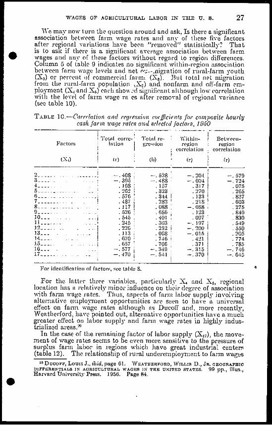

~
I l5
TADLB l1-Signijicant correlations betwren compos1te hourly cash farm wage rate and selected factors 1950
Fnetorsns~oclated with Fllctors assoclntcd with the supplr or rarm blhor the demand ror rarm
tljlabor
Popuilltion chmgcq NonlIgrlculluTIII elll Extent or opermiddot COlllpo~ltc ployment atlons ~
honrlyEconom Ie regions wugc
TIlle Percentllgc Perccntlgc Percentage ~ lotllinet Agc~ 15middotlU I Rcplilcemiddot nongrlmiddot operators Econ IPercentage I-migration net mlgrn ment Tlltlo enlturnl w100+ CiBSS I rarms with I-tlon or men ngcd employmiddot dnys olTshy I [ rarms tractors 01
25-69 ment rlmn work ~01
Correlation coelficiwuCent ~ United Stntcs bullbullbull __ ~bull_bullbullbullbullbull 52
VIII Southenst Constal Plllln __ 35 -~ 500 _ ~~ ~ _ 584 492 _ __ ____ ___ _ Jl VII 43 __ __ bull bull ~g 4211 bull2Ill
X sect~~tfth~~~e~~rS~Yt~~~~tmiddotLiill 44 __ __ bullbull bullbull ~ bullbullbullbullbull ~ -424 _ 381 740 ~ IV Upper Oreul Lnkes bullbullbull__ ~ __bullbullbull__ ____ 44 740 700 - tlSO bull 855 bull SGtmiddot ___ -005- l L Atlantic Filltwoods ltd dnH COllsL _ 48 bullbullbull_ ~ bullbull __ -800 542 _ _ If Ellslern Grellt ]Ilkes nnd Northeast Uplnnd 53 __ bull ~ ~ ~_ HO ~ V North Cenler (Corn Belt) ____ 53 _bullbullbull __ 294
III Lower Oroot Lllkcs M _~_ ~ -452 -62 _ _ _ ~ 515- 686 o VI Centml Phlns 60 _ w _~ ~ _-lt __ ~ _~_ ~ ~_ - ~ _~ ~ _~~~~ ___ -yen __ gt1 __ ~
I Atlnntic Mctropolltan nelL 61 ~ _~ ~ -72nmiddotmiddot 50- ~ ~ 1))5 XI Hocky Monntaln and Intcrmollntllin ~ ~ tH -444 ____ ~ __ -450 44 gt xu Pllclnc Northll(middotst bull ____ ~ _~ ~ bullbull __ ~ 81 __ ~ ~ __ __
xur Pllcillc SOllthwcst ~ 81 -806 ~ __ _ _bullbull
Only stntistiCIIlly ~lgnlncanL corrclllUons lIf(l I~tcd -slgnlficnnt lit lhe 001 level -significant lit the 01 level -slgnillcllllt lit the 051evcl I bull bull
bull bull
TABLE ll-Significant correlations between composite hourly cash farm wage mte and selectecl factors 1950-Continued ~ o lj mFnctors BSSoclntcd with the demnnd for farm Inhor
Farmmiddotoperntor fumll level-ofmiddot o living Indexes l
Abllltymiddotlomiddotpay JImiddot~poundtockCompositeEconomic regions hourly
~ cwago Percontnge Avemge
rote commercial size of farms arm Vlne VIIIIIO Valne )crcon ttlge Percellt
land nnd products livestock livestock 1l4O IUSO chllnge buildings sold per fllrm Is of sales 1040-1050
Correolion coelicienlJOel1U United Statcs bull___bullbullbull 52
Vln Southcast Coastal Plllln __ 15 VII Centml BOd Eastern Upland 41 =~~~~ ~~=~~ ==1== l~i~i ~~~ ~~~ =~~~
tllX Soutb Center and Southwest Plnlns ____ bull 44 728 lJ(l(l 420 bull [() 55l 846 821l -700 oIV Upper Oreat Lukes___ bullbullbullbullbullbull 44 DC Atllwtlc Flutwoods Ilnd Gnlf Const 48 II Eastern Orent Lllkcs and N orthetlst Upland 53 ~~~ 1~~~~~ -~~I~~~~ ~~~~ ~=~~~ ~~ c V N ortb Ccnter (Corn Delt)__ ___ il ----- -- --_- - ~ ---- ~ 1- - - -_ ~ Z~ ~ ~~ ~
III Lower Orent Lnkes __ 54 __ _______ h8 551 _ bull71 GII 11l7 -011 VI Centrnl Plnlns (10 _ ___ ___ _ ____ 3i2- _ __ __ _ _ _ __ ~ ~ 56-1 5ramiddotmiddotmiddot _
I Atlantic MetropolltBII Dell 01 ___________ - itUmiddot 510middot n04middotmiddot _ _ ___ _ _ 810middot i45middot -001middotmiddotmiddot XI Rocky rfonntnln nnd Intermouutllln 04 ~ XII Pncillc Northwestbullbullbullbullbullbull___ 81
XUI Pacillc SouUmmiddotest_ __ 81 ~ ~~~~ ~~~I-~~- ~
Only statistically slgnlllcnnt correlations are listed middot-slgnlficullt at the 001 level -slgnIIlCIIllt at tbe 01 level -Slb111flCIIllt nt the 05 level l
~ ~
------
--
Co)TABLE 12-Regr(ssioll cnlttJicirnts oj (olnpo8poundlr hourly c(1sharln W(1C rate~ on sliertedJactrmjor 13 economic regions1 1950 ~
-E-RO-e~-li-~~l-liC-r ~2 I X3 XI XI X6 middotx ~R Xu i Xlo Xli X I2 T~l rI~-r~~~-r~-l-~- ~ ------_-~----J~I----2-I-s --81~i--l-U~5~-~~----1--8-~17i-1~~-5-J-n-5 5I()j -21(1----0-0-31--r-5-1
-shyL __________ _
1 ImiddotW - GnO - 1 Olfi ~ [L ~---r----ou~ 252---ilJ~2G2i--~55~()Ul-~2I(r~-5()-I---12r - 0771=1 middotJJl~-7middotIU--- - middot155 amp070 -077 tlt---1------ - --------~-- ------------ ---_-----------
toIII_ --- __ -~3l-middot6If 058- 088i middotI~ii 2Gul IllS 7501 ii20-30001 aI)I-a12 711 middot S(nl - J38 - IJ5S
~middot--middot=middotrl22ii-middot-Gi--~72Imiddot-----S2ur=-middot~72= 5uol- 5l(ii~middot~~75i=middot(07-1 ]-251-1 1101- S571- 5l5 -715 (3lt] - nlill E Y--- _ ___1- 223--Oi2j-osuj-GU1r-0621--1middot16 --006-- 0221 o5-i-- llltf-1111-middot 1121--228 23G -23U -OJI
VI ___ --li5l-lll-2261-177j-1middoti31 -026 = 0I2-~ izl OSt~middot12Grmiddot- 12i1-~10al-m 553 -1()5 -1(S Z
_1Y-r-I------1----170j-~-2-fi-ll--middot2-0-si~-I-1S(--2~5t~-07-5 =- OS~~~-S-5-2- 2 i--2Ii --middot~-22-al--l(jlj--2-5-0 223 -067 -14l -1
15jVHT__ -_- 1)68- 2~ ~l 101_middot_middot~~1 ~_~i-lI~~- 1~8~~1 1001 573 middot j3a -OSU -154 IX --1-170-073 middot12 7J5i OmiddotI- 0l21- 001 105 laGI ])1 00L 0551 80J middot aso -285 -611
rIl
- t) r ~--middot-I-----~--I-~--~-l--~(-i---- middot1 ) 1------I I -2gt11 - a12X ____ bull _ o~o_~~__~~~r~_~~(_~~-~~ 1 ~)1_1_ 30~~_ 8n~ t1
d middot XL _ __ 1- nO3l 1371 3middot1 q ll- 2-171 1lG 020- 111 -2151-280 -210- llii 134 1 -00middot1 -1Jl o I------i---------I---I------ ------- --middot~i--- middot tjXII __1-20~- 31~1 0--1) 001-0141-002 (ll2 01) 0~Sbull 03) w6S 0~SI 11 l -118 -oa6
middot o 1 - middot 375 -1 oun -087 lX~~I~___-J~ ~3ISl--middot-1Rj--1- 2721~~ a121-307-- 524= ()~l3- 262 5001 - 70(ii-middot_-l~I ___~~~i---
gt
-+--~-~-~- - - - ~ shy 8For idcntificnbioll of fH~tor li tnble S ~
~ tltl
bull bull
35 WAGES OF AGRICULTURAL LABOR IN THE U s
these perquisites arc not included in the computation of the composite hourly wage Tute (Sec Appendix B)
bull The Atlantic ~Ietropolitan Belt (Economic Region I) runks next to
the Lower GTeat Lnkes region in the proportion of rw-ul-farm popushylation engaged in nonagricult urnl or off-farm work Thile the proshyportion of commercial farms here is low the proportion of Economic Class I I1nd II farms is high Farming operntiolls in this region consist largely of dall- truck or mixed fn Iming n nel capitn1 im-estshyment and yalue of production nrc rclnth-cly high Among the rurnlshyfnrm population 1940-50 net migllltioll and 1950-60 replacement ratios -ere rclntiYely low (fig ~) But fnrm -nges showed a tendency to decline with increnses in the 1950-GO replnecment rnLio for alCn ngecl 25-69 and (0 rise with incrcnses in the proportion of nonngrishy(uiturnl employnlPnt Ynges n1so tended (0 be higher where the proportion of Economic Clnss I I1nd II fnrlllS wns high and where the ynIue of lnud nncI buildings tlw ynlue of ploduds sold nnd fO1I11shyoperator fUTni1 leY(~l-of-liying indexes were high On the other hand there wns 11 st ronger inyerse 1(]11ionship between fnrm wflges nncl size of furm (in aercs) in this region (table 11) Dniry fl1rms makQ up u subslantial pnrt of the large aerenges in this region nut t1uel fnrms dominnte the medium- nnd smnll-size groups The reliltiYely low monthly (1sh wa~e rut(s on dnir- fntms tend to pull down the ayernge wnge on the lnrgel fnrllls while the smnlier truck farms usunllr p1~- the rell1th-ely high picce nnd homl- Inles
Regions V nBc VI hilye the highcst proportion of (onl1l1(r(ial fnrl1ls of nny purt of lhe eountry Hegion V the North (enter Corn Belt is noted for the ptodudion of feed grnins and liyesloek llegion 1 the Centrul Plains produces most of the nnlions whent nncI slllull grains (fig 2) FnIming in these regions is done on It lnrgc scnle -illl high (apitnI iIlY(stn1Cnt ilnd hi~h aYClnge -olue of plmiddotodtHtioll Xonshyngriculturnl alld off-fnrm employment umong the 1urnl-fnrm popushylation is locl ]1(re thun n11-wh0re in the countlY Net migrntion from the rurnl-fnrJll population nntI Lite leplnC(IJllent lntio for lIlen nged 25-09 -erc low in the Corn Belt III the Centrnl PIn ins toUd net migml ion fOm the rUlnl-fiuJ1l populn lion alld the lCplnCclIl(llt mtio for men nged 25-(j) en hi~h hut IIct oUi-Jnigrntion of the 15-19 nge group wus low
In Economic Regions nl1d Y1 fllrllling opernliolls nrc fnidshyuniform tluoughoul tIll Stntc e(onomic illens In the COlll BrIt fnIm wages tended to be]tighel wli(re the proportion of farms haying t1ncil)1s wns high In Lhe (eltml PInins wnges -pre highrl where YIIlue of hmd and huildings wns high nnd -here [he fnrm-opcrnfol fnmily level-of-li-illg ilHlcx ns hi~h Thlse -cre the onL) slnt islishyraly significant Ielntiollships obsclTed ill thrse I(gions I)((ren the level of wages and the selrcted suppl- und demnnd foetols find of these only the nssocintion between wngr rntes find the fnllIl-opellltor family level-of-Iiying index in the Ccn(rnl ])Ininsleuthcd the OOlley(1 of significance (table ll)
The Rocky ~rolin tnin and In tcrmoulltain Region XI is the princi pnl livestock rnnge in the countJmiddoty with some irlignt(d Hens producing special crops including cotton cgetnblrs nnd sugnr brcts H(le
bull arc found the largpst farms and needkss to sny the highest TtlhlCs of liVestoek pel fnl1I1 Cnpitul ir1Yestmcnt nnd nlue of production
wTABLE 13-Region means in composite howmiddotty cash fann weLge rates amd other selected factors 361 State economic areas ~
1950 gt-3
Economic regions Variable Unit of All
measure Ie- ~ gions I II III IV V VI VII IVIII IX X XI XII Xl] I C gtt
CenL________XI Composite hourly wage 52 61 f4middot 54 4middot1 53 60 43 35 48 44 64 81 8 tlj cjrate
X2 Rate of net out-migra- Percent- _____ 29 21 20 20 28 26 34 29 35 33 45 30 18 16 tion from the total ~
gt-3rural-farm population1940-50 ~
X3 Rate of net out-migra- Perccnt ______ 58 45 47 51 54 46 50 58 61 56 68 50 50 36 tion from the 1940 -Irural-farm population -I
aged 15-19 1940-50 X Percent of rural-farm PercenL _____ 29 17 42 48 22 18 12 35 28 34 22 21 -10 2 9 c
population employed in nonagricultural inshy ~ dustries 1950 11Percent______Xs Percent of farm oper- 25 33 34 37 20 14 13 2n 22 34 22 27 38 31 tl
stors reporting 100 or ~ more days of off-farm work in 1949 o
XI Average value of land Thousand 158 168 9 6 119 96 22 5 260 6 9 5 4 170 10 7 274 23 4 42 5 J
and buildings per dollars gt Glfarm 1950 0PercentX7 Percent of farms report- ______ 51 54 56 62 71 75 80 26 21 32 37 56 60 54
ing tractors 1950 Percent ______Xe Percent commercial 68 64 63 60 79 87 89 51 62 52 67 72 58 71
falms comprised of all ifarms 1950 0PercenL _____ 20 2 19 16 26 tlXli Percent Economic Class 11 18 11 6 4 17 2 9 7 I and II farms comshyprised of all farms 1950
bull bull
bull bull XI Average value of proshy
ducts sold per farm 1950
X11 Average size of farm in acres 1950
Xn Average value of liveshystock per farm 1950
XI3 Percent livestock and livestock products are of all products sold 1950
X l4 Farm-operator family level-of-livingindeCl940
XIS Farm-operator family level-of-living index1950
X l6 Percentage change in farm-operator family level-of-living indexes 1940-50
Xu Replacement ratio for rural-farm men in working age group25-69 1950-60
T bousand 49 6 5 45 3 2 34 6 4 dollars
~res ________A 240 88 137 96 139 188
T bousand 2 8 18 23 17 2 8 34 dollars3rcent______P 57 64 77 68 84 70
u S Mean= 83 115 109 109 97 117 100
u S Mean = 124 153 151 142 138 160 100
P 3rccnt______ 68 38 38 31 46 39
lrcenL _____P 134 114 118 117 119 118
--~-----
78
876
5 5
53
92
141
56
142
17
102
12
68
51
90
96
137
17
98
7
30
37
76
116
176
53
269
2 5
36
52
103
104
152
a I
172
16
37
44
87
124
137
79
1332
9 0
67
95
185
43
143
5 iI
269
19
48
114
153
34
98
14 i
5lii
4 1
38
137
182
3a
117
~ ~ o j
shy~
~ o d t
~ ltI gt t
~ ~ ltI
rz ~ tj
~ YJ
C) -t
38 TECHNICAL BULLETIN 1177 U S DEPT OF AGRICULTURE
arc also relatively high Nonagricultural employment is relatively low but there is a high proportion of farm operators who work 100 or more ditys off the farm As in the Central Plains total net outmiddot migrntion from the llual-fann populntion and the replacement ratio bull for men in the working age group ere high but net migmtion of the 15-19 age group was low (fig 3) Here however the farm wage level appears to be significantly associlLtecl with the leyd of total net migrntion being lorer in State economic areas bere out-migration is highcr lhele wns a slight tendency for farlll wages to be higher whclC the plOporticn of tractor ownership Vas high 1he relationship behctn the composite wage rnte and most of the otlwr labor demand 1ncLors vas negfttiyo LOer farm wage rates were associated with hig-ber proportions of Economic Olass I and II farms higher yahlCs of It1i1cl and buildings higher yalues of products sold larger farms and higher valne of licstock per farm The liLrge stod ranches appear to hae 10cr aye rage wage rates tlLan the slllaller Ycgetable sugar bect and gClltrnl farms in the region But llono of these associations reached the 00l1tYcl of statistical signific~Ulce (table ll)
In the higlHmiddotnge Paciiic Northwest region no signiiicant associashytions between the composite rage rate ancl any of the other factors (rc ohserved lfuch of thc tcrritory in this region is nonfarm area sp((inliz(cl wheat growing arc a is in the northern part of the region and tlHre nlso are some dnirr poultr and mixed farming areas and some of fruit nnd mixed farming rJw proportion of eomnwTcial farms is smnll but the proportion of Eeonomic Class I and II farms is largp Fnrming is done Oil a llrge scnJp with hig acrengps high capital irrveshncnt and high lLlllO of proc1uetion Among thc rumlshyfnrm population 1l01lngrieultu1nl (rnplonn(nt wns relatiyely high Rntps of net olll-migmtion lnd rpplnCellltnt of mpn aged 25-69 wore rompnmtiwly low (fig 3)
The Pacific Southwest is noted for its fruit truCk and mixed flIJlling areas 1gtu t it also contains SOJ11( arcns that spccilllizc in small grains irrigntlCl eotton clairing and (xtensiYe litnge livcstock opeLntions ict out-mignttioLl and replneement rntios Hre very 10 alllong the rural-fnrl1l population in this region KonagrieulLuml employmrnt was neftI the nntionnl average and 11 eompamtiycly Inrgc numbcl 01 fnllll OWIators did 100 or more days of off-farm work Fuming is clolH Oll it laqp seah with litrge fftlms high capital inshyvcstmcrlt and high alue of production
] n this high age region farm wages yore lligher when the 1950-60 replacemcnt mtio for mPH ag(cl 25-09 was 10 among th( rural-farm population Vng(s wore loer in Stte economic areas haying high nvcrngt vnhws of livestock per farm and ages wele 10c] OIl 1mge 1n Ims as in tIle Rocky) fountain and IutpllllolllltlLin l(lgion
CONCLUSIONS AND IMPLICATIONS
This aJHtlysis has d(mOJlsLnLt(cl lhe II ide regional disparity in cash farm wng( riLLes and the eompkxity of faelors tlwt influence these differences Not oilly do fiLllll mg(s yary glCaUy fro111 one 10culiLy to another ItS has been iJldiclLLed U)T wage statistics for maDY years bu t it is evident that shltrp vnrintions (xist in tbe chnmcLeristics of fl1dmiddotors und(dying these loeal und l(gioJlltl diiieLCJl tinls In some bull
WAGES OF AGRICULTURAL LABOR IN THE U s 39
areas population variables and other clements of labor supply wcre
bull founel to be closely associated with villiations in cash farm wage rates In others aspects of the demand for fmm labor appeared to be molC closely linked to the level of falm wl1gc ratcs In some of the ccoshynomic rcgions studied nonc 01 vcry few of the scleetcd variables appel1lccl to be signifieantJy ldated to variations in (ash farm wage rates Whether the lack of slalisUcnl I1ssoCialion ill these e(onomic regions CUll be nttributed to locnl peculil1rities stntisticnl variatioJl or other reasons is not clear Perhn])s thr SN1SOJlltl varinLion which I1ccollnted for abou t hl11f of the incrcase ill fnrm wages bttecn the spring of 1950 and tbe fall of ] 954 has con trilgtlI teel su bstan tinlly to the regiollal pnHem of signiflC[Ult llssocilLtiOJIS JllOclueecl by the analysis As W( 1)11v( s((n the fnJI flllIll wllgt picture vl1li(s regionally from the spring wage pattCrn An al1nlysis of the nlntionship bebreen fall rates and fudols of Inhor demand and supply might provide widely clifiel(ll t re3ulls
Since the casb age rnL(s reported foJ April largelY represent wngcs of rpgular allet rclativel)-long-tCrm farm workers lhe chances arc good that the long-run dfpets of rural mlglation and tUlclelemploym(llL have grcater influence on April than on faU ntge rates The fnU rates reflect [he wagts of J1llU1Y sbort-tcrm scasollnl farm workers as con trusted yiib those of rogular long-limE -olko1s ill A])lil III April 1954 f((I than a fifth of nll farm -olk(ls we]( nOllfarm lcsidenis22 y( call assume that the figure ould be much higher during th( fall hillvest SlUSOll 1 [ost of thesc -o1kPls am )-ouths housewives alld cldcJly ])(r50J1S who 11( dmwll i))io Hw hbol force only during periods of heny dCnllulCl fol InboJ It is likely that tllC wages of seasonal farm olkels anclrlglllaJ farm workers arc influeJl(NI by a common sd ofittetors of lahor cl(tlulJld such as seale of op(rutions and valuc of products solel Yd it is plo]Hlhle (bat in ppriods of p(ak dClllal1d fol farm lahor (omlitiollS or labol supply in nonfarm lahor 11uukcis-thc sou ref of 11111(11 sNlSOllnl farm bbor-oycrshnclow the effects of UJ(leICmplo)-n1(nt altclllathc job opporhUlitips and othor aspects of lIra] labor SlII)ply on the ]PYel of fnlm wage rates
Tllis study Ilns shown that lhe moYemfnls of farm wagc riLles Hlld ext011 L of aHernatiHI employmell t opportunities g()1ellllly coincide througbout tbe country D(spito the suhstanlial gains in farm wagc levels during Tecen t years farm wage ratcs are not cOll1petiti-c with industrial wage s([lles YlHll industrial jobs are nyailable nenrllY rural residents arc l1ttrnctrd nay from farlll johs and pounde-er lIonfarm residc)) ts arc likc]y to seck farm (mploYllleJ1 L
The Jlature of the relationship bcLwecn far111 wnge rates and rural unccrcwploymclI t appears to yar~- ngionally In a rN1S dose to nonfarm 80urCes of clllployment farm wagc rates arc muCli morc sensitiye to changes in the supp- of fnrm lahor thall they are jn preclominnntly ruml ill(llS Hoe-cl this relationship is sOllwlimEs modified by special conc1i lions of labor d(ll111nd III regions in which the lcquirclUcmts for hirecllnbor rise steeply for r(la tinl~- short pcriods fatm wage 1n(es also nrc sPllsitiyo to chmlgps ill the leyei of rural undercll1ploymon t
bull n Computed from data in FAn~r PO l UITlOX Neries CenlIs-AiIR P-~7
No 20 1)51 ancl from ANNUM REiPOHl ON TllE [Anon FOnGI) Ifl54 Bureau of the Census Current Population Series P-50 No 59
40 TECHNICAL BULLE~lN lI7i U S DEPT OF AGRICULTURE
There can he no doubt that hired farm workers as a group are neaf the bottom of the income pyramid in the Ulilted States It is far less clear wbat can and should be done about it The character of Amerishycan agriculture particularly in the South is undergoing swift and bull dramatic change Policies that apPC1U to offer solutions to todays problems may be ineffectual under tomollOWS conditions The marginal character of a substantial part of the hired farm work force makes it particularly difficult to shape a clear-cut policy with reshyspect to farm labor Strikingly different are the problems of tbe displaced sharecropper for example from those of the high school student working on a farm (humiddotjng summer vacation
The establishment of the Rurnl Development Program alld othor concerted efforts Lo raise rural levels of Jiv-ing are evidellce of the growing concern over the problcm of low farm incomes Farm wages are another aspect of the problem that deservcs the attention of all those concerned with the imprOYCmlllt of the agricnltull1l economy and rural li-ing
TABLE 14-Compo~ite houriy cash jann wage Tates alul number oj hired jarm workers by economic lcgion8 States and State economic area8 1950 and 1954
I 19-0 1954)
--_ Composite Number Composite Number
hourly of hired hourly of hired wage rate workers wage rate workers
rell~ Thollsand~ Genis IThollsandsl-nited States________________ _I 52 ]525 79 2730Economic regions I
I Atlantic Metropolitall I iBelt________________ _
I GO 117 84 157
II Eastern Great Lak(gts and 1 N orthenstern cpl1nd __ 53 83 167
I 881In Lower Grent Lakes_____ _ 57 57 84 103IV cpper Great Lakes _____ _ II 43 49 I 75 76 V North Center (Corn Belt)_ t 52 168 81 2]4
VI Gentml Plail1S __________ 1 G1 76 I 87 I 157 VII Central and Eastern Upshyland _________________1 41 138 16061 tVnI Southeast Coastal Plain__ 33 242 49 432 IX Atlantic Flatwoods and
Gulf Coast__________ l 154 64 13348 j X South Ceuter and South- I wcst Plains ___________ 1 41 Hil 60 578
XI Rocky IVfountaiu and I Intermountain________ I 62 I 69 78 Wl
XII Pacific Northlest _______1 82 40 108 i 76XnI Pacific SouthwesL______ bull 84 171 3161 100 1States and State economic areas Alabama ____________ bull _____ 32 3-( I 48 G9Area L _______________ 29 6 40 14Area 2 ________________ 1 37 2 50 9
Areas 3 and A ________ _ 41 i 2 i 60 G
bull
41 WAGES OF AGRICULTURAL LABOR IN lHE U s
TABLE 14-Composite hou1ly cash farm wage rates and number of
bull hired farm 11)0rkers by economic regions States and State economic areas 1950 and 1954--Contilluecl
1950 1954 i ____--____--------_
Area Iii Composite I Xumber Composite Xumber
hourly I of hired I hourly of hired wage rate workers I wage rlte workers
------------- ------Btates and State economic
arens-Continued Alabama-Continued Cents Thollsands Cents IThousands
~Ireas 4 ltnd 13______ 29 2 43 3Area 5______ bull __ bull ___ -_ 31 5 43 I 9 Area 6 and C _______ 30 9 40 I 11Area 7a __ __________ 29 7 47( 13Area 7b _____ bull _ __ bull 41 1 48 1Arens 8 and D ________ _ 47 3 64 3
Arizona_______ bull __ ____ 68 10 79 48Area 1____ _ __ _ __ __ 61 1 83 1 Area A ___ ____ __ 70 8middot 81 14 Area 2a _____ _ 5 I68 76 25 Area 2b ___ bull ___ _ 64 2 i 79 8
Arkansas ______ ___ bull _ 38 43 55 149Area la ___ _ ______ __ 51 2 66 1Area 1b ___ ________ _ 44 1 01 1Area 2____ - ____ ____ ~_middot 13 I 1 63 3 Areas 3 and A ____ __ 41 3 61 5Area 4__ ________ _ 50 t 66 1Area 5 ____________ bull 34 31 50 5Area 6 _____________ _ 40 I 60 I 5 Area 7lL___________ __ 38 I 59 47Area 7b ______ __ ~ 1141 53 7Area 8abullbull______ _ _ 36 15 50 58Area 8b _____________ bull 35 I 5 51 16
California ____________ S6 161 102 278Area 1 __________ ___ __ 91 2 115 4 Area 2_____ __ _ bull 88 4 103 10 Areas A and 13 _____ _ 91 15 103 35Area 3_______________ 82 14 101 17 Areas ~ and C____ _ __ i 89 13 113 26 Areas () and D ________ _ 9U 18 107 38 Areas6audE___ __ j 83 39 101 80 Areas 7 F G and H ___ 92 34 106 43Area 8 ________________ 74 19 90 21Area 9______________ __ 79 3 103 4Colorado_________________ bull 54 19 87 36 Area 1_______ - - ---i 56 2 86 3Area 2a_______________ 61 2 86 6Area 2b ____________ _ 58 2 86 10Area3______ bull ________ 68 5 89 6 Areas 4 and A____ __1 92 5Area 5______ bull ____ __ 60 77 6
Connecticut_____ 73 11
71 971 13Areas 1 and A__ 70 3 89 2 Areas 13 and C ___ _ 79 5 99 8Area 2___ _ 69 3 i 98 3
Delaware__ 59 I 84 64 Areas 1 and iL 59 I 41 84 6
bull
42 rECHNICAL BULLETLlt 11 i i J U S DEPT OF AORICULlURE
TABLE l4-00mposite hourly cash jarm wage rates and number oj hired jarm workers by economic 1egions States wnd State economic areas 1950 and 1954-Contillued
1950 1954I bull1-----shy 1----1 1AreH Composite I Number IComposite IXumber hourly of hired I hourl of hiredj wage mt( orkers i wag( rilte workers
------------i 1 --- shy
otates and Btate economic i I areas-Continued Cents Thousandsl Cellis ThousandsFloridlL__________ _ 57 j6 74 48Area L __ _ 42 1 G5 2Areas 2 and A__ _ j GO 4 77 2Area 3 _________ _ 35 15 51 10Area 4 ___ _ 67 4 81 4--JAreas 5 and B___ 64 21 80 16Areas 6 and C__ _ 62 21 81 14Georgia_________ 32 03 48 63Areas 1 and A__ _ 30 gt 56 4Area 2____ _ _ -In 62 1 Areas 3 and B 43 ~ I 4AJ-eIL 4a_____ _ 32 7
62 I 7Area 4b____ _ 36 middot1 ~r I 4
Areas 5 C and D __ 31 1 4 348 IArea 6_____ _ _ _ 30 I 7 43 I 10AreIL 7a ____ _ 25 6 37 8Area 7b_____ _ 30 13 42 12Area 8____ 32 13 46 9Arem 9 and E __ _ j1 3 59 1
Idaho __ 73 12 102 29real ___ _ G5 2 3Area 2 ____ _ G7 1 19~ I 1Area 3a ____ _ 73 3 I 95 7Area 3b ___ _ 3 71 99 j 6Aree 1 ___ _ 79 3 12108Illi nois __ _ 53 49 t 82 1 54Areai 1 A and B __ 5G 5 I 86 71rCllR 2 und C__ _ 7 G6 l2 8Arell 3 __ _ 50 6 83 7Area -1 _____ _ 49 5 j 74 5ArCH 5 __ _ gt 56 l6 3 reuR 6a D and E 55 81 6Area 6b ___ _ 51 gl 81 9Areas 7 [uld F_ 46 74 3Area 8___ _ 50 rI 72 1Arell 9 __ _ 47 2 68 2Area 10____ _ 50 1 72 1Area 1 L ____ - 46 2 65 2
IndianlL_____ __shy 53 27 81 37 Arens I A and B ___ 64 83 3Area 2a________ bull _ _ 05 3 90 4Area 2b_____ ___ _ 52 4 84 6Arens 3 and C__ _ 51 872 3Aren 4__ bull ________ 0 59 3 85 5Areas 5 and D____ _ 51 5 80 6Areas 6 and E __ 51 4 72Area 7 ______ bull __ 45 I 72
5 3
Areas 8 and F_ 44 2 70 2
bull
WACES OF ACRlCGLfURAL LABOR L~ THE U s 43
TABLE l4-Composite hourly cash fann wage mtesand number of
bull hiled farm workers by economic regions States amd State economic areas 1950 and 1954-Continued
1950 1954
Area CompOHite IKumber IComposite Ii ~ulllberI hourly of hired I hourl of hired I wage ritte _ worken wage rate I workerI I____ ____
I States and State economic i
areas-Continued Cellts IIwusundsl Gellts ITholl~ands Iowa__________ _ 53 39 82 48
Area la_________ -- o-lt) 4 i 83 i 5 Areas Ib A und B_ 56 6 1 83 6 Area 2a______ - __ _ 50 2 81 3 Areas 2b and C___ _ 5li 6 85 8 Area 3a____ _ 51 2 84 3 Area 3b_____ 51 2 2
74Area 4___ _ 50 6 77 8 Area 5____ 54 5 86 6 Arells 6 and D_ 53 6 84 7
Kansu(______ __ 62 18 1 01 j 27 Area L ____ 67 3 90 4 _~rea 2a~_ _ t 65 3 97 5
97 Area 2L ___ _ 67 1 2 Areas 3a and A 64 2 92 3 Area 3b____ _ 71 1 92 1j
Area 4___ _ 56 1 90 2 Area 5___ _ 62 2 85 3 Areas 6 and 13 ____ _ 56 3 89 4 Area 711 _____ 1 85 258 Arell 7b____ _ 57 1 82 I 1
Ken tucky __ bull 39 43 62 bull 58 ArCti L__ 39 2 68 4 Area 2 ___ _ 36 51 I 2 Area 3a____ _ 33 53 i 3 Area 3b ___ _ 31 3~I Area 4___ bull 30 5 i ~~ I i Area 5bull 33 4 5 Arel~ 6 A and 13_ I 13 G740 471 20 Area 7bullbull __ 54 7 75 10 Areas 8 and C __ _ 38 3 54 5 Ar~t 9 ___ _ 44 2 1
56 ILouisiantl 38 ~12 55 108 Arefl~ 1 und A__ 34 5 53 19 )rea2___ _ 35 6 47 27
lt)-Area 3 __ 37 1 3 I 56 0 Arro 4 __ __ 3G 1 71 5 Areas 5 11IIeI 13 ___ ) 58 6 Area u_ 5037 1 ]3 55 16 Area 7___ _ 42 4 62 8 Area 8_ __ 1 66 240 I[aine__ _ 67 9 93 46 Area L __ _ 75 I 4 111 35 Area 2 ___ _ 59 I 2 85 5 Area 3___ _ 61 1 Ul 2 Areas 4 and A 62 2 4I 84 1
[arylancL___ 49 i 21 73 22 Area L __ _ 47 (I) 74 I 1 Area 2__ _ 46 (j 69 t
1 L(S8 Lim n 500bullbull 6
44 TECHNICAL BULLETL 1177 U S DBPT OF AGRICULTURE
45 WAGES OF AGRICULTURAL LABOR IN THE U~ s
TABLE 14--0ornposite hourly cash farm wage ates and number oj
bull hired farm workers by economic 1egions Stales and State economi( areas 1950 and 1954-Continued
1950 HJ54
Area compositel Kumber Composite
hourly of hired I hourly wage riite workers I wage rnte
- -lt--_----------
States and State economic areas-Continued
JIissouri-ConLinued CenlN Tholls(lndbullbull (enlbull Area 1___ 3 I 73 Area 5bull middotHi GO Arens 0 and B lt16 i 4 72
IArea 7__ 411 1 3 G7 Area 8___ middotIG 1 03jArea 9a __ _ 38 I 2 51 Area 9b 3U i
I 5 i 57 IontamL _ 00
j 12 84 Area la___ 1 61 i 1 H2 Area 1IL ___ 02 3 82 Are 2nbull_ 50 2 87 Area 2IL_ _ middot -1 (j2 3 87 - Area 31 ___ -- - 03 I 78 Area 3IL ___
~
745l 2IXebraslm_
50 10 SO-- ---Area L ____ ~)2 3 80 Area 2_bull
- bullbull middot1 G3 2 00 Aret 311 ___ 55 82 Area aIL ____ 51 2middot 70~==I
Area 4___ (i2 J 2 80 Area 5_ (iij 89 Area (j ___ ijO i 78 Arets 7 A nlld -13~=--- Ii) ~ SOxevada_____ __ Ga ~ so Area 1____ G3 3 SO
Xc IIamphire ( 5 SG ArelL ] ____ 51 2 J 87 Arets 2 and A G7 3 8(j
Xew Tersey____ bull I (i7 23 86 Areas I A B und C GS 12 III Areas 2 D E 11l11 F Gij 11 83
X(w Jexieo __ __ li2 12 1 G7 Area Itl __ GO 1 71 Area lb____ -J 1
iJ~ GlArea 2____ - )3 3 70Area 3~ ____ __ 50 7 1 62
New York__ ____ ~ r 55 52 87 Arens I A nud 13 __ (3 7 80 Area 2____ _ -middot1 4 stAren 311_____ 411 3 87 Area 3b_____ 5middot1 3 HO Areas 4 nnd C _ 51 5 t 85Areas 5 nnd D _____ 4ii 3 I 71 ArelLs 0 and E _ 46 5 j 65 Arel1 7 ____ (j 7448 Arens 8 nne I ii2 3 77 ArCiL 0_____ )7 m s I
bull Area G SO 5 104
Kumber of hired workers
I I t Thou~a1ds I I
1
3 2 1 (l
2) 17
1 4 3 5 2 2
20 4 G 4
2I 3
2 2 a a 3 5 2 3
35 15 20 3G 2 2 0
26 94 21
9 9 0 7 4 4 7 3
15j 9
46 TECHNICAL BULLETlK 1177 U S DEPT OF AGRICULTURE
TABLE l4-Composite hou1ly cash farm wage rateB and number oj hired farm workers by economic regions States and State economic areas 1950 ancl1954-Continucd
-----------------~----~-----
1950 195middot bull Area
States and lltate ecollolllic areas-Continued
North Carolina Areas 1 and A Area Z_ bull _ Areas 3 Band C Area 4abullbull _ Area 4bbull_ Areas 5 and D __ bull Areas 6 and E__ _ Area 7__ _ _ Area 8 __ Area 9 _bullbullbull __ _ Area 10 ____ Area 11__ bull ___ _
Xorth Dakota_ __ Area L___ Area 23_____ _ Area 21gt ___ _ Area 3ll ____ Area 3b __ _ Area 3( bull __ Area L ___ _
Ohio ____ _ Arcus 1 and A Area Z Aren~ 3 B C lWei D Areu 4a and R Area 4b ____ Areas 5 F G and II Area 6a______ Areas 6b and J _ Area~ 7 and JL Area SIt and L_ Area Sb __
Oklahoma bullbullbullbull Area L Area 2 bullbull Arell5 3 and AArea 4 ____ bull Area 5 and B Area 6 __ Area 7a Area 7b __ Area 8a Area 8b _ _ Area g __
Oregoll Area 1a Area Ihbull _ Areas 2a a Illi ~
i Composite i Number I houri of hiredwage rute orkers
((Jl(~
40 middotW middot1 65 1 -l7 oj 37 1 -)v_ 2 39 4 3D ) 31 6 34 S 35 4 42 3 38 l 56 1 54 2 67 1 1
50 1 56 Z 4J 2 J7 64 2 55 33 )[1 3 56 3 )4 l 74 3 47 2 fil 4 53 2 43 2 4R 3 44 2 43 2 gt5 ]8 67 2 6n 2 i6 ~
61 il 57 3 43 1 48 1 41 ]
4Z 1 39 1 42 1 79 20 77 1 82 2 SO S
CompOHitehourly
wage rilte
(tlliN
56 60 73 63 61 64 57 54 53 57
50 56 53 87 73 89 75 77 73 72 I
102 86 12 87 87 12 76 n3 SI 78 82 64 62 78 II 92 70 81 80 02 76 00 58 64 58
105 105 100 102
Number of hired workers
Thollsa IrL~ )l
3 1 6 2
4 13 18 16
8 -
14 33
3 Z 2 6 4 2
14 48
6 4
11 4 3 7 3 3 3 2 2
63 5 middot1 4
28 6 2 3 4 4
(1) 3
38 2 2
20 Les than 500 bull I
47 WAGES OF AGRICULTURAL LABOR IN THE U s
TABLE a-Oomposite Murly cash farm wage rates and number of
bull hired farm workers by economic regions States and State economic areas 1950 and 1954-Continued
1950
Area Composite Number Composite Number
hourly of hired hourly of hired wage rate workers wage rate workers
iStates and State economic
areas-Continued Oregon-Continued Crnts IThou~and~ Clnl~ ThousfLndsArea 2b _______ _ 84 2 103 4Area 3 _______ 76 2 103 2Area 4 ________ _ 78 5 ]07 8Pennsylvania________ _ )2 16 7n 72
Areas la A and B 53 3 87 7Area lb________ _ H) 2 87 3Area 2 _________ _ 42 4 72 5Area 3________ bull ____ 45 ] 71 1Area ___________ 69 2 Areas 4b and E__ _ 67 3Areas 5 and F _____ 19 I ~ 44 4 68 5 Areas 6 G and C __ 48 4 72 8Areas 7 and H ____ _ 50 I 4 77 9Area D___________ 50 I 3 80 4Areas J and K ______ I 4J I 5 80 8 Areas L 1II and N_ 60 1 ]3 87 17
Rhode Island_____ __ _ 68 1 2 97 IAreas] and A___ _ 68 1 2 97 1
South Carolina __ _ 30 1 14 43 58Area L ____ _ middot16 ] 51 1Area 2____ _ 41 I 5 48 4Area 3___ _ 33 2 44 2Area 4_______ _ 30 3 42 3 Areas 5 A and B bullbull 32 4 60 3Area 6____ 24 17 37 29Area 7____ 26 (i 38 ] 1 Areas 8 and C__ _ 35 6 52 5
Souih Dakota__ 5] 11 79 18Area L __ _ 54 3 75 4Area 2a _____ _ 53 ] 76 2 Area 2b_ __ 56 2 82 4Area 3a ___ _ 52 1 74 1 Area 3b __ 52 1 81 2Area 4a____ _ 50 1 82 2 Area 4b __ _ 55 2 80 3
Tennes~ee____ _ 33 45 liZ 100Arens 1 and A __ _ 3 13 49 57Aren 2 ___ _ 36 I 2 61 11 Area 3_____ __ bull 36 2 51 4Area 4_____ _ 37 3 50 3 Arens 5 and B___ 31 9 44 7Area 6__________ 30 3 47 5Area 7_______ _ 37 1 55 2 Arens 8a C and D_ 40 5 55 5Area 8b________ 30 7 46 6TeAas ____ ______ 44 146 62 346 Areas la and A __ 46 7 54 35Area lb____ 42 4 )4 j
bull Area 2 _____ 57 4 70 Ii
48 TECHNICAL BULLETIN 1177 U S DEPT OF AGRICULTURE
TABLE 14-00mposite hourly cash farm wage rates and number of hired farm workers by economic regions States and State economic areas 1950 ancl1954-Continued
Ul50 1954 bull_______~-------i-------~-----Area Composite I Number I Composite Number
I hourly of hired hourly of hired Iage rate I___middoto_rk_e_r_s_ wage rate workers
-------------- ---------~I--------Rtates and Slate economic
areas-Contin ued Texas-Continued Cents Thollsands Cents Thollsands
Area 3____ ___ __ - 40 10 51 9Area 4____ ___ _ 61 5 81 20Area 5____ _bullbull 52 7 73 54Area Gu ___ _ 56 9 74 42Area 6b ____ ] 8059 2Area 7a_____ 59 2 73 3AreaR 7b and B ___ 58 1 3 76 6Area 7e ____________ _ 52 I 2 71 2 Areas 8 CJ D and E 11 19 57 73Area L ________ _ 38 I 5 57 14Area] 0_________ 15 3 58 6Areas] 1 and 1__ _ 47 1 59 9Area ]2_____ bull __ - __ 10 2245 I 111 62Area 13____________ 48 i 1 70 4 Areal 14 G and J1__ 54 i 10 72 17Area 15______ 32 33 47 17CtaIL _______ 76 7 93 ]4Area L___ __ 75 I 3 )4 3 AreaR 2 and A_ i7 2 88 7Area 3__ ______ __ H 2 )n 4(rmont ________ ____ _ 47 8 75 10Area 1 _______________ 1 43 3 65 4 bull
Aca 2______ _ 50 5 83 6 1Ig1ll11l _____ __ __ 43 I 44 50 5)Area L _________ _ 3fi 2 45 2
_rea 2 ___ bull ___ 38 I 5 48 4 reas 3 and A__ _ bullG 3 63 3 Area 4____ bull 47 5 fi8 8Area 5 and B__ 441 8 fiO 8 rea 6 aud C __ ) 62 741 IArea 7 __- 42 584 6Areas 8 und n___ __ 53 3 70 3Area 10___ __ 35 544 10 Areas 11 and D _ 5 58 8WUhington ______ bull __ 47183 23 117 42Area 1__ _____ _ 82 1 123 1Area 2_______ 70 2 102 4 Areas 3 A lnd B_ __ 83 3 114 5 Areas 4 and C____ 81 1 104 2Area 5a_______ ____ bull 85 3 116 10Area 5b__________ bull __ bull 7) () )7 1Area 6____________ __ _ 85 8 ]08 12Area 711______ _ 86 2 1]3 3Areas 7b and D ______ _ 7) 3 108 4
rest Virginia____________ l 45 12 63 12Areas 1 and A _______ _ 47 1 60 1Areas 2a and B_______ _j 2 156441Area 2b_______ bullbull __ _ 40 2 2 61
Less than 500 bull
49 WAGES OF AGRICULTURAL LABOR IN lHE U s
TABLE 14-Composite hourly cash farm wage rates and number of
bull hired farm workers by economic regions States and State economic areas 1950 and 1954-Continued
1l50 1l54
Area IComposite Number I Composite II Kumber hourly of hired hourly of hired------------1 wage rate __o_rk_e_r_s_I wage rate __o_rk_c_rs_
States and State economic i I are~-Continned I
West Virginia-Continued l Ce111s Thousands Cents ThollsandsArea 3 __________ __ j 47 1 64 1Areas 4 and C______ __ 56 1 70Area 5 ______________ 1 44 3 61 3Area 6 ____________ bull __ _ 47 2 71 4Wisconsin ____________ ___ _ 41 37 73 51Areas 1 and A__ _____ _ 52 2 93 TArea 2a_____ __ ___ bull 38 4 62 5 Area 2b _____ _ 37 3 66 3Area 3_______ bull _ _ bull 39 3 64 3 Area 4_____ - ____ - _-1 36 3 79 7Area 5 _______________ 38 2 73 3Area 6 ________________ 1 37 3 6l 4
__ -- --I 6Area 7______ bull --- 3l 5 62 Areas 8 and B_ _ I 44 10 6l 10 Areas land C_____ ___ 54 2 89 3
Wyoming_________ bull _ 60 7 7l 8Area 1__________ bull ____ 01 3 72 2Area 211_______ bullbull __ _ 62 2 85 3Area 2b _______ ____ 57 2 l 70 3
1 I 1 Less than 500 Number of hired workers from Cen1uses of Agriculture In50 and 1954 Compo-ite hourly wage rate5 computed by Agricult1lral Marketing Service from
data in Censuses of Agriculture 105f) and 1 l54
APPENDIX A COMPARISON OF FARM WAGE EXPENDITURE AND WAGE RATE DATA IN THE CENSUSES OF AGRICULTURE FOR 1940 1945 1950 AND 1954 AND WAGE RATE DATA IN THE AMS FARM WAGE SERIES Information on farm wage expenditures in the Censuses of Agriculshy
ture for 1940 1945 1050 aDd 1954 farm -age rate data in the Censuses of A~Ticulture for 1950 and 1954 and the farm wage series of the Agricultural Marketing Selyice difler in scyeml D1ajvr respects The dtfinitioll of hired farm labor the method of reporting wage inshyformation the geographic area for which wage information is reported size of sample and method of enumemtion and the date to which the data relate
The 1940 and 1945 Censuses of Agriculture define hired farm workers as persOns 14 years of age and oyer who worked two or more days at farm wage work during specified weeks which closely approximated
bull the beginning of the enumeration
50 TECHNICAL BULLETIN 1177 U S DEPT OF AGRICULTURE
The 1950 and 1954 Censuses of AOriculture and the l1gricultural Shrketing Service define hired farm 1abor as aIL persons doing 1 or more hours of farm work Oi chores for pay during the survey week ~1embers of the operators family doing farm work for cash wages are bull counted as hired workers Croppers arc considered family workers when working on their own crops but hired workers when doing farm work for payoff their own tracts If a pprson is emplo~ed both as a family worker and a hired worker during the survey week on the same farm he is counled as a hired worker In lhe A~1S farm labor series wage rates are reported quarterly by the same sample of farm operators that reports em ploymcnt The fanner is asked lo rrpolt average wage rates being paiel teat this time ill his 10tality teAt this time on the anrage probably represents the second or third dar before the pnd of the month
III 1940 the Census of Agriculture reported Lhe numbrr of workers b- the b1sis on which the~- err hired during the specified week(a) By the month (b) by the day or week or (c) other (including pieceshywork and contmct labor) lh(l 1945 census reported only total number of hired farm workrrs during the specified week In both 1940 and 1945 lhe ClnSllSrS published the aggregate cash wage bill in thl pnvious year III addition number of farllls was reported by a bllukdown of total wage bill per farm in the previous year
In 1950 and 1954 tile Census of Agriculture reported hired farm workers by basis of pnymlnt (monthly Heldy daily hourly pieceshywork) anrage wage per month week day or hour and average hours I)(r month week or clu~ In 1950 there was fill additional breakdown of number of farms by P(l(l uisitCs furnished worker paid on a monthly ((ldy or daily basis which mlS not obtained in the Census of ~gricultur( for 1954 This still varies somewhat from the A~IS Farm Lnbor series 11ic11 r(ports average rates being paid to hired farm labor in the locality on a monthly eekl~ daily or hourly bnsis yith and without board nnd room or house
Gross farm mge rxpenditulls were reported for counties States nnd geogmphic divisions in the 1940 1945 1950 and 1954 agricultural censuses The 1950 nnll 1954 censuses reported fann wage rate data by State e(onomie anas States and geographic divisions The AMS farm nlampe rate data is leportlcl for States and geographic divisions
Agrieulluml IIarketing Service rstimatEs nrc based on mailrd qUlstionllairEs received each month from 20000 to 25000 farmers who rlport the llumber of ptrSOl1S working on their farms during the last (Omplele ealendar -((k Cnding at lcast one day before the end of the 111011 th Yage Ta les arc reporlrd quarterly by the same sample of farm operators The furmer is askrd to report average wage ral(s bcmiddoting paid lIut this tjme in his loenlity The Censlls of Agriculture is based 011 a sHmple of 20 percent or more of all farm operators
For the 1940 Census of AgriCuliur( the specified reporting weeks (rc )1arch 24-30 in 1940 with census date of April 1 and the week pnding January 6 IJl 1945 wilh census date of January 1 (The Ilvemgc date of enumeration in 1945 was March 16-31)
For 1950 the Census of Agriculture wage rates and numbers elllshyployed related to the week prrceding the enullleration For 43 States the ayeruge date of enumeration was April 15-28 for the reshymaining 5 Slatrs l11r IlY(IIlge dntr wns April 1-14 For 1954 tIw bull
51 WAGES OF AGRICULTURAL LABOR IN poundHE U s
Oensus of Agriculture wage rates and numbers employed related to a
bull specific week For 33 States the week was September 26-0ctober 2 while for the other 15 States the week was October 24-30
APPENDIX B METHOD OF COMPUTATION OF THE COMPOSITE HOURLY CASH FARM WAGE RATES
Tile 1950 and 1954 Oensuses of Agriculture Vol I Oounties and State Economic Areas Parts 1 to 33 list for each State economic area in the United States the following information on hired farm workers by 1lt~sis of payment Paid on a monthly basis-persons Paid on a daily basis-persons
average hours worked per month average hours worked per day average wage per month (dollars) average wage per day (dollars)
Paid on a weekly basis-persons Paid on an hourly basis-persons average hours worked per week average wage per hour (dollars) ayerage wage per week (dollars) Paid on a piece-work basis-persons
The composite hourly wage rate was computed as follows 1 age rates other than hourly rates were converted to an hourly equivalent
by dividing total wages in basis of payment group by the average hours worked 2 These hourly-equivalent rates were then weighted by the number of workerR
in the corresponding basis of payment groups giving the gross hourly wage bill for each group The average hourly rate was weighted by the number of pieceshyrate workers as well as hourly workers to obtain an estimated wage bill for piece workers
3 These products were then totaled according to the ares for which a composite wage rate was desired For one State economic area the gross hourly wage bills for all the different bases of payment were summed and then divided by the total number of workers in the area to obtain the composite hourly wage rate The gums of these products for all State economic areas were added together and then divided by the total number of workers in a State to obtain the composite rate for each State The same procedure was used to obtain composite hourly wage rates for each economic region
The composite hourly wage rates computed in this manner represhysent cash payments only and do not include the vnlue of perquisites furnished in addition to cash wages
APPENDIX C DEFINITIONS AND EXPLANATIONS OF SELECTED FACTORS COMPARED WITH COMPOSITE HOURLY CASH FARM WAGE RATES All of the quantities 01 values involved in the selected economic
and demographic factors that were compared with composite hourly cash fann wage rates were computed for State economic areas State economic aren indexes of actual values of these factors were grouped or averaged to obtain the broader geographic area averages
X 2 Rate of net out-migration from the total lulal1al1n l)opulation 1940-50
The estimates of net out-migration of persons from the rural-farm population between 1940 and 1950 relate to persons alive in both 1940 and 1950 and do not include estimates of migration of those born or dying during the decade Net migration is expressed as a percentage
bull of the e-pectecl survivors to 1950 of persons living on rural farms in
52 TECENICAL BULLEiIN 1177 U S DEP1 OJ AGRICULTURE
1940 (See BOWLES GLADYS K FARM POPULATION-NET MIGRATION FROM THE RURAL-FARM POPULATION 1940-50 Statistical Bulletin No 176 U S Dept Agr 1956) Oensus forward survival ratios were applied to 1940 sex-age-color groups of 1940 rural-farm popula- bull tion obtnined by summing appropriate county dnta from the 1940 Oensus of Populntion to obtl1in the population e1gt-pected to be alive in 1950 The difference between these estimates of expected survivors and the actual rurnl-farm population aged 10 and over residing in each State economic area in 1950 was obtained These lesults were the estimates of net migration which were then related to the expected population
X3 Rate oj net out-migration jrom the 1940 1Ural-jwm population aged 15-19 1940-50
The estimates of net out-migrntion of persons nged15-19 from the nUal-farm population betwerll 1940 and 1950 relnte to persons nged 15-19 in 1940 alive in both 1940 nud 1950 and do not include estishymatIS of migll1tion of persons aged 15-19 in 1940 rho died during the drcacLc Net migration of persons aged 15-19 is e1gt-pressed as a pershycentage of persons nged 15-19 living on rUInl farms in 1940 expected to survive fmd reach ages 25-29 in 1950 The method of computashytion is the samc itS that used to obtain total net migration in item X 2 bull
X 4 Percent oj 1UTClZ-jalJn p01J1llation employed in nonagriculi1tral inshy(hlstrie8 1950
Number of persons in the lUlnl-larm population emplored in nonshyagricultural industries in 1950 expressed as a percentage of totnl emshyployed nm1l-furm population For State economic nreas in 44 States this percentage middota8 computed from unpublished data in the 1950 Oensus of Population on employment by industry groups among the rurnl-farm population 14 years old and over by counties For 8tate economic areas in Alabama Iowa Louisi[1))a and Virginia data were used from Vol II Ohap B Tnble 49 of the 1950 Oensus of Populashytiol1 showing employment by major occupation groups
X5 Percent oj farm operators reporting 100 or more days oj oif-ja1m worlc in 1949
Farm operators report-iug 100 or more clays off-farm work ill 1949 expressed as a percentage of tOt1 farm operators in 1950 Off-farm work means either nOllagricultlUal employment or work on a farm other than the oprrators o-n for cash wages (1950 Oensus of Agrishyeultmc Vol T Oounties and State Economic Alens Economic Alea Table 1 line 7 Farm opemtors working off their farms 100 days or more divided by line 1 Number of farms)
Xa Average value oj land and bulclings per jarm 1950 Total value of land und buildings divided by the total number of
farms (1950 Oensus of Agricultme Vol I Oounties and State Economic Areas Economic Area Table 5 (Part 1 of 2) line 12)
bull
53 WAGES OF AGRlCULTURAL LABOR IN THE U s
X 7 Percent oj jarms reporting tractors 1950 Number of faTms having tractors expressed as a percelltage of the
bull total IitIllber oHarms (1950 Oensus of Agriculture Vol I Oounties and State Economic Meas Economic Area Table 5 (Part 2 of 2) line 16 divided by line l)
X g Percent commercial jarrns comprised oj all jarms 1950 Nmnber of commercial farms e)-pressed as S) percentage of the total
number of farms Commercial farms are all farms vith a yalue of sales of farm products amounting to $1200 and farms witb a yalue of sales of $250 io $1199 if tbe farm operator worked off the farm less than 100 days and the income whirh the farm operator and memshybers of his fmllily received from nonfarm SOLuces was less than the total alue of alr farm producls sold (H150 Census of Agriculture Vol I Coun ties and SULte EeonoIuic Areas Economic Area Table S (Part 1 of 2) lille 1 TotaL commereial farms dhidecl by Total aU farms)
Xo Percent Economic Class I and II farms comprised oj all jarms 1950
Number of farms havin~ value of prQ(Lucts sold of $10000 or more -pressed as a percellla~e of the lotal number of farms (1950 Censhysus of Agricultme Yo1 I COlLies and SlaLe Economic Arcas Ecoshynomic ALCa Table 8 (Part 1 of 2) liM 1 Class I plus Class II diTidecl by Total all fnrms)
XO Average value oj Jr()dllct~ 80ld pOfa rill 1[J50 rotnl Yillue of farm products sol(1 diided hJ~ tolal lHlllllwl of farms
(1950 Census of Agrieultull Yol 1 COllnli(s alld Slnte Economic Areas Economic AlCtl TallIe 9 lillP 3 (li-id(d by Eeollomic 1rta Tnblc 1 line 1 for the South Economic Aren TabLe 9 lill( 34 diyided by line 1 Economic ArN1 Table 1 for other Stat(s)
Xli Average size rdfarm ill ([erN 1tJ50 ToLal number of ncn ill fnrms dividld h-lhe totalllLunbeJ of fllrm~
0950 C(l)SUS of Agriclillnlo Yo1 I COlmties find Rtllie Economic Arens Economic ArCll Tul)Itl G (Pnrl 1 of 2 lille 9)
12 Avemge vahle ojliN8IocklJCljarm 1750 ToLlll vulur of speciii((l classes of Jiwslock (horsCs llwles cHLlie
hogs shCep chickens and turke)s) cliYidpcl h)- Lotllinumher of farms (1950 Census of Agriculture Yo1 1 Counties nJld Stftt( Economi( Areas CounLy Table 4 (Part 1 of 2) liJ1e 1 wns gr()u)rd into Stale economic nreas and divided by Economic Area Tuble 1 Lille 1)
X 13 Percent livestock and livestocle p7Oduct8 are of alll)ro(1lcts 8old 1950 Value of livestork nml lin-sloek products sold ()l)ressed fiS a
pcrceltage of total v111ue of brm products sold (1950 Census of Agricultme VoL I Counties and Slotl Eco1lomic Anas Ecollomie Area Table 9 Line lt1l cliided b)T liDO 8ii for till Routh lil1l 40 c1iic1lcl hy line 84 for olher RtoJrs)
bull
54 TECHNICAL BULLETIN 1177 U S DEPT O AGRICULTURE
X a 15 Fcmn-opelator jamily level-oj-living indexes 1940 and 1950 Level-oi-living indexes for farm operator families by counties an
based on the following items (1) Percentage of farms with electricity (2) percentage of farms wi til telephones (3) percentage of farms bull with automobiles and (4) average value of products sold or traded ill the preceding calendar year (adjusted for chnnges in purchasing power of the farmers dollar) Indexes for ~tate economic areas are simple arithmetic a-eragcs of lIte iUdexes for the counties in the State economic meas The County and State economic area level-of-living indexes used ill this stud and 1 desceiption of their computation arc IOlmd in HAGOOD lAHGAHEr JAIUrAX FAHlIf-OPEHATOH PAULY LEYEL-OF-LIYTNG- INDXES Fon COGNlIES OF Trff~ UNrrElD STArJS 1930 1940 1945 AND 1950 Bureau of Agticulturnl Economics U S DeptAgr WashiJJgtoll 1952
XI6 Percentage chal1ge in farm-operator faliiily lad-of-living indofs 1940-50
Diffcrence betwctll 1940 1IJld 1950 lcV(J-of-lijllg iJl(Iltxes (~pl(ss(das a l)crccntage of thc 1940 indtx
XI Replacement ratio ful rUlaliarm litelt in 1vorkillg age group f5-69 1950-60
rlhis latio indicates the IlumbN of young llWU 15-24 ill the nuul-farm population in 1950 dJO will be cntCring the -oJkiug age group Ior evlY 100 older men who will die or retire b(tween 1950 and 1960 Tto higber this replacement ratio the greater is tht cxcess of men entering the -orking age group o-cr the mUllbe ne(ckd to replace those moring out of this group (BOWLES GLADYS K Bnd TABrnmt COXHAD HUHAL-FAHM MAfJES EX1EHTXr AXD JJ~AYIXG WOHKIXr AGES 1940-50 AXD 1950-60 -HgPLACEJ~Xl RATWS AXD HATES lodes Census-A~D (P-21) ~o 22 Gil pp Ynsldngton 195G)
U GOVERNNEfIT RlNtINltO 1JFrICE IHO bull
bull
t I

bull bull
TABLE ll-Significant correlations between composite hourly cash farm wage mte and selectecl factors 1950-Continued ~ o lj mFnctors BSSoclntcd with the demnnd for farm Inhor
Farmmiddotoperntor fumll level-ofmiddot o living Indexes l
Abllltymiddotlomiddotpay JImiddot~poundtockCompositeEconomic regions hourly
~ cwago Percontnge Avemge
rote commercial size of farms arm Vlne VIIIIIO Valne )crcon ttlge Percellt
land nnd products livestock livestock 1l4O IUSO chllnge buildings sold per fllrm Is of sales 1040-1050
Correolion coelicienlJOel1U United Statcs bull___bullbullbull 52
Vln Southcast Coastal Plllln __ 15 VII Centml BOd Eastern Upland 41 =~~~~ ~~=~~ ==1== l~i~i ~~~ ~~~ =~~~
tllX Soutb Center and Southwest Plnlns ____ bull 44 728 lJ(l(l 420 bull [() 55l 846 821l -700 oIV Upper Oreat Lukes___ bullbullbullbullbullbull 44 DC Atllwtlc Flutwoods Ilnd Gnlf Const 48 II Eastern Orent Lllkcs and N orthetlst Upland 53 ~~~ 1~~~~~ -~~I~~~~ ~~~~ ~=~~~ ~~ c V N ortb Ccnter (Corn Delt)__ ___ il ----- -- --_- - ~ ---- ~ 1- - - -_ ~ Z~ ~ ~~ ~
III Lower Orent Lnkes __ 54 __ _______ h8 551 _ bull71 GII 11l7 -011 VI Centrnl Plnlns (10 _ ___ ___ _ ____ 3i2- _ __ __ _ _ _ __ ~ ~ 56-1 5ramiddotmiddotmiddot _
I Atlantic MetropolltBII Dell 01 ___________ - itUmiddot 510middot n04middotmiddot _ _ ___ _ _ 810middot i45middot -001middotmiddotmiddot XI Rocky rfonntnln nnd Intermouutllln 04 ~ XII Pncillc Northwestbullbullbullbullbullbull___ 81
XUI Pacillc SouUmmiddotest_ __ 81 ~ ~~~~ ~~~I-~~- ~
Only statistically slgnlllcnnt correlations are listed middot-slgnlficullt at the 001 level -slgnIIlCIIllt at tbe 01 level -Slb111flCIIllt nt the 05 level l
~ ~
------
--
Co)TABLE 12-Regr(ssioll cnlttJicirnts oj (olnpo8poundlr hourly c(1sharln W(1C rate~ on sliertedJactrmjor 13 economic regions1 1950 ~
-E-RO-e~-li-~~l-liC-r ~2 I X3 XI XI X6 middotx ~R Xu i Xlo Xli X I2 T~l rI~-r~~~-r~-l-~- ~ ------_-~----J~I----2-I-s --81~i--l-U~5~-~~----1--8-~17i-1~~-5-J-n-5 5I()j -21(1----0-0-31--r-5-1
-shyL __________ _
1 ImiddotW - GnO - 1 Olfi ~ [L ~---r----ou~ 252---ilJ~2G2i--~55~()Ul-~2I(r~-5()-I---12r - 0771=1 middotJJl~-7middotIU--- - middot155 amp070 -077 tlt---1------ - --------~-- ------------ ---_-----------
toIII_ --- __ -~3l-middot6If 058- 088i middotI~ii 2Gul IllS 7501 ii20-30001 aI)I-a12 711 middot S(nl - J38 - IJ5S
~middot--middot=middotrl22ii-middot-Gi--~72Imiddot-----S2ur=-middot~72= 5uol- 5l(ii~middot~~75i=middot(07-1 ]-251-1 1101- S571- 5l5 -715 (3lt] - nlill E Y--- _ ___1- 223--Oi2j-osuj-GU1r-0621--1middot16 --006-- 0221 o5-i-- llltf-1111-middot 1121--228 23G -23U -OJI
VI ___ --li5l-lll-2261-177j-1middoti31 -026 = 0I2-~ izl OSt~middot12Grmiddot- 12i1-~10al-m 553 -1()5 -1(S Z
_1Y-r-I------1----170j-~-2-fi-ll--middot2-0-si~-I-1S(--2~5t~-07-5 =- OS~~~-S-5-2- 2 i--2Ii --middot~-22-al--l(jlj--2-5-0 223 -067 -14l -1
15jVHT__ -_- 1)68- 2~ ~l 101_middot_middot~~1 ~_~i-lI~~- 1~8~~1 1001 573 middot j3a -OSU -154 IX --1-170-073 middot12 7J5i OmiddotI- 0l21- 001 105 laGI ])1 00L 0551 80J middot aso -285 -611
rIl
- t) r ~--middot-I-----~--I-~--~-l--~(-i---- middot1 ) 1------I I -2gt11 - a12X ____ bull _ o~o_~~__~~~r~_~~(_~~-~~ 1 ~)1_1_ 30~~_ 8n~ t1
d middot XL _ __ 1- nO3l 1371 3middot1 q ll- 2-171 1lG 020- 111 -2151-280 -210- llii 134 1 -00middot1 -1Jl o I------i---------I---I------ ------- --middot~i--- middot tjXII __1-20~- 31~1 0--1) 001-0141-002 (ll2 01) 0~Sbull 03) w6S 0~SI 11 l -118 -oa6
middot o 1 - middot 375 -1 oun -087 lX~~I~___-J~ ~3ISl--middot-1Rj--1- 2721~~ a121-307-- 524= ()~l3- 262 5001 - 70(ii-middot_-l~I ___~~~i---
gt
-+--~-~-~- - - - ~ shy 8For idcntificnbioll of fH~tor li tnble S ~
~ tltl
bull bull
35 WAGES OF AGRICULTURAL LABOR IN THE U s
these perquisites arc not included in the computation of the composite hourly wage Tute (Sec Appendix B)
bull The Atlantic ~Ietropolitan Belt (Economic Region I) runks next to
the Lower GTeat Lnkes region in the proportion of rw-ul-farm popushylation engaged in nonagricult urnl or off-farm work Thile the proshyportion of commercial farms here is low the proportion of Economic Class I I1nd II farms is high Farming operntiolls in this region consist largely of dall- truck or mixed fn Iming n nel capitn1 im-estshyment and yalue of production nrc rclnth-cly high Among the rurnlshyfnrm population 1940-50 net migllltioll and 1950-60 replacement ratios -ere rclntiYely low (fig ~) But fnrm -nges showed a tendency to decline with increnses in the 1950-GO replnecment rnLio for alCn ngecl 25-69 and (0 rise with incrcnses in the proportion of nonngrishy(uiturnl employnlPnt Ynges n1so tended (0 be higher where the proportion of Economic Clnss I I1nd II fnrlllS wns high and where the ynIue of lnud nncI buildings tlw ynlue of ploduds sold nnd fO1I11shyoperator fUTni1 leY(~l-of-liying indexes were high On the other hand there wns 11 st ronger inyerse 1(]11ionship between fnrm wflges nncl size of furm (in aercs) in this region (table 11) Dniry fl1rms makQ up u subslantial pnrt of the large aerenges in this region nut t1uel fnrms dominnte the medium- nnd smnll-size groups The reliltiYely low monthly (1sh wa~e rut(s on dnir- fntms tend to pull down the ayernge wnge on the lnrgel fnrllls while the smnlier truck farms usunllr p1~- the rell1th-ely high picce nnd homl- Inles
Regions V nBc VI hilye the highcst proportion of (onl1l1(r(ial fnrl1ls of nny purt of lhe eountry Hegion V the North (enter Corn Belt is noted for the ptodudion of feed grnins and liyesloek llegion 1 the Centrul Plains produces most of the nnlions whent nncI slllull grains (fig 2) FnIming in these regions is done on It lnrgc scnle -illl high (apitnI iIlY(stn1Cnt ilnd hi~h aYClnge -olue of plmiddotodtHtioll Xonshyngriculturnl alld off-fnrm employment umong the 1urnl-fnrm popushylation is locl ]1(re thun n11-wh0re in the countlY Net migrntion from the rurnl-fnrJll population nntI Lite leplnC(IJllent lntio for lIlen nged 25-09 -erc low in the Corn Belt III the Centrnl PIn ins toUd net migml ion fOm the rUlnl-fiuJ1l populn lion alld the lCplnCclIl(llt mtio for men nged 25-(j) en hi~h hut IIct oUi-Jnigrntion of the 15-19 nge group wus low
In Economic Regions nl1d Y1 fllrllling opernliolls nrc fnidshyuniform tluoughoul tIll Stntc e(onomic illens In the COlll BrIt fnIm wages tended to be]tighel wli(re the proportion of farms haying t1ncil)1s wns high In Lhe (eltml PInins wnges -pre highrl where YIIlue of hmd and huildings wns high nnd -here [he fnrm-opcrnfol fnmily level-of-li-illg ilHlcx ns hi~h Thlse -cre the onL) slnt islishyraly significant Ielntiollships obsclTed ill thrse I(gions I)((ren the level of wages and the selrcted suppl- und demnnd foetols find of these only the nssocintion between wngr rntes find the fnllIl-opellltor family level-of-Iiying index in the Ccn(rnl ])Ininsleuthcd the OOlley(1 of significance (table ll)
The Rocky ~rolin tnin and In tcrmoulltain Region XI is the princi pnl livestock rnnge in the countJmiddoty with some irlignt(d Hens producing special crops including cotton cgetnblrs nnd sugnr brcts H(le
bull arc found the largpst farms and needkss to sny the highest TtlhlCs of liVestoek pel fnl1I1 Cnpitul ir1Yestmcnt nnd nlue of production
wTABLE 13-Region means in composite howmiddotty cash fann weLge rates amd other selected factors 361 State economic areas ~
1950 gt-3
Economic regions Variable Unit of All
measure Ie- ~ gions I II III IV V VI VII IVIII IX X XI XII Xl] I C gtt
CenL________XI Composite hourly wage 52 61 f4middot 54 4middot1 53 60 43 35 48 44 64 81 8 tlj cjrate
X2 Rate of net out-migra- Percent- _____ 29 21 20 20 28 26 34 29 35 33 45 30 18 16 tion from the total ~
gt-3rural-farm population1940-50 ~
X3 Rate of net out-migra- Perccnt ______ 58 45 47 51 54 46 50 58 61 56 68 50 50 36 tion from the 1940 -Irural-farm population -I
aged 15-19 1940-50 X Percent of rural-farm PercenL _____ 29 17 42 48 22 18 12 35 28 34 22 21 -10 2 9 c
population employed in nonagricultural inshy ~ dustries 1950 11Percent______Xs Percent of farm oper- 25 33 34 37 20 14 13 2n 22 34 22 27 38 31 tl
stors reporting 100 or ~ more days of off-farm work in 1949 o
XI Average value of land Thousand 158 168 9 6 119 96 22 5 260 6 9 5 4 170 10 7 274 23 4 42 5 J
and buildings per dollars gt Glfarm 1950 0PercentX7 Percent of farms report- ______ 51 54 56 62 71 75 80 26 21 32 37 56 60 54
ing tractors 1950 Percent ______Xe Percent commercial 68 64 63 60 79 87 89 51 62 52 67 72 58 71
falms comprised of all ifarms 1950 0PercenL _____ 20 2 19 16 26 tlXli Percent Economic Class 11 18 11 6 4 17 2 9 7 I and II farms comshyprised of all farms 1950
bull bull
bull bull XI Average value of proshy
ducts sold per farm 1950
X11 Average size of farm in acres 1950
Xn Average value of liveshystock per farm 1950
XI3 Percent livestock and livestock products are of all products sold 1950
X l4 Farm-operator family level-of-livingindeCl940
XIS Farm-operator family level-of-living index1950
X l6 Percentage change in farm-operator family level-of-living indexes 1940-50
Xu Replacement ratio for rural-farm men in working age group25-69 1950-60
T bousand 49 6 5 45 3 2 34 6 4 dollars
~res ________A 240 88 137 96 139 188
T bousand 2 8 18 23 17 2 8 34 dollars3rcent______P 57 64 77 68 84 70
u S Mean= 83 115 109 109 97 117 100
u S Mean = 124 153 151 142 138 160 100
P 3rccnt______ 68 38 38 31 46 39
lrcenL _____P 134 114 118 117 119 118
--~-----
78
876
5 5
53
92
141
56
142
17
102
12
68
51
90
96
137
17
98
7
30
37
76
116
176
53
269
2 5
36
52
103
104
152
a I
172
16
37
44
87
124
137
79
1332
9 0
67
95
185
43
143
5 iI
269
19
48
114
153
34
98
14 i
5lii
4 1
38
137
182
3a
117
~ ~ o j
shy~
~ o d t
~ ltI gt t
~ ~ ltI
rz ~ tj
~ YJ
C) -t
38 TECHNICAL BULLETIN 1177 U S DEPT OF AGRICULTURE
arc also relatively high Nonagricultural employment is relatively low but there is a high proportion of farm operators who work 100 or more ditys off the farm As in the Central Plains total net outmiddot migrntion from the llual-fann populntion and the replacement ratio bull for men in the working age group ere high but net migmtion of the 15-19 age group was low (fig 3) Here however the farm wage level appears to be significantly associlLtecl with the leyd of total net migrntion being lorer in State economic areas bere out-migration is highcr lhele wns a slight tendency for farlll wages to be higher whclC the plOporticn of tractor ownership Vas high 1he relationship behctn the composite wage rnte and most of the otlwr labor demand 1ncLors vas negfttiyo LOer farm wage rates were associated with hig-ber proportions of Economic Olass I and II farms higher yahlCs of It1i1cl and buildings higher yalues of products sold larger farms and higher valne of licstock per farm The liLrge stod ranches appear to hae 10cr aye rage wage rates tlLan the slllaller Ycgetable sugar bect and gClltrnl farms in the region But llono of these associations reached the 00l1tYcl of statistical signific~Ulce (table ll)
In the higlHmiddotnge Paciiic Northwest region no signiiicant associashytions between the composite rage rate ancl any of the other factors (rc ohserved lfuch of thc tcrritory in this region is nonfarm area sp((inliz(cl wheat growing arc a is in the northern part of the region and tlHre nlso are some dnirr poultr and mixed farming areas and some of fruit nnd mixed farming rJw proportion of eomnwTcial farms is smnll but the proportion of Eeonomic Class I and II farms is largp Fnrming is done Oil a llrge scnJp with hig acrengps high capital irrveshncnt and high lLlllO of proc1uetion Among thc rumlshyfnrm population 1l01lngrieultu1nl (rnplonn(nt wns relatiyely high Rntps of net olll-migmtion lnd rpplnCellltnt of mpn aged 25-69 wore rompnmtiwly low (fig 3)
The Pacific Southwest is noted for its fruit truCk and mixed flIJlling areas 1gtu t it also contains SOJ11( arcns that spccilllizc in small grains irrigntlCl eotton clairing and (xtensiYe litnge livcstock opeLntions ict out-mignttioLl and replneement rntios Hre very 10 alllong the rural-fnrl1l population in this region KonagrieulLuml employmrnt was neftI the nntionnl average and 11 eompamtiycly Inrgc numbcl 01 fnllll OWIators did 100 or more days of off-farm work Fuming is clolH Oll it laqp seah with litrge fftlms high capital inshyvcstmcrlt and high alue of production
] n this high age region farm wages yore lligher when the 1950-60 replacemcnt mtio for mPH ag(cl 25-09 was 10 among th( rural-farm population Vng(s wore loer in Stte economic areas haying high nvcrngt vnhws of livestock per farm and ages wele 10c] OIl 1mge 1n Ims as in tIle Rocky) fountain and IutpllllolllltlLin l(lgion
CONCLUSIONS AND IMPLICATIONS
This aJHtlysis has d(mOJlsLnLt(cl lhe II ide regional disparity in cash farm wng( riLLes and the eompkxity of faelors tlwt influence these differences Not oilly do fiLllll mg(s yary glCaUy fro111 one 10culiLy to another ItS has been iJldiclLLed U)T wage statistics for maDY years bu t it is evident that shltrp vnrintions (xist in tbe chnmcLeristics of fl1dmiddotors und(dying these loeal und l(gioJlltl diiieLCJl tinls In some bull
WAGES OF AGRICULTURAL LABOR IN THE U s 39
areas population variables and other clements of labor supply wcre
bull founel to be closely associated with villiations in cash farm wage rates In others aspects of the demand for fmm labor appeared to be molC closely linked to the level of falm wl1gc ratcs In some of the ccoshynomic rcgions studied nonc 01 vcry few of the scleetcd variables appel1lccl to be signifieantJy ldated to variations in (ash farm wage rates Whether the lack of slalisUcnl I1ssoCialion ill these e(onomic regions CUll be nttributed to locnl peculil1rities stntisticnl variatioJl or other reasons is not clear Perhn])s thr SN1SOJlltl varinLion which I1ccollnted for abou t hl11f of the incrcase ill fnrm wages bttecn the spring of 1950 and tbe fall of ] 954 has con trilgtlI teel su bstan tinlly to the regiollal pnHem of signiflC[Ult llssocilLtiOJIS JllOclueecl by the analysis As W( 1)11v( s((n the fnJI flllIll wllgt picture vl1li(s regionally from the spring wage pattCrn An al1nlysis of the nlntionship bebreen fall rates and fudols of Inhor demand and supply might provide widely clifiel(ll t re3ulls
Since the casb age rnL(s reported foJ April largelY represent wngcs of rpgular allet rclativel)-long-tCrm farm workers lhe chances arc good that the long-run dfpets of rural mlglation and tUlclelemploym(llL have grcater influence on April than on faU ntge rates The fnU rates reflect [he wagts of J1llU1Y sbort-tcrm scasollnl farm workers as con trusted yiib those of rogular long-limE -olko1s ill A])lil III April 1954 f((I than a fifth of nll farm -olk(ls we]( nOllfarm lcsidenis22 y( call assume that the figure ould be much higher during th( fall hillvest SlUSOll 1 [ost of thesc -o1kPls am )-ouths housewives alld cldcJly ])(r50J1S who 11( dmwll i))io Hw hbol force only during periods of heny dCnllulCl fol InboJ It is likely that tllC wages of seasonal farm olkels anclrlglllaJ farm workers arc influeJl(NI by a common sd ofittetors of lahor cl(tlulJld such as seale of op(rutions and valuc of products solel Yd it is plo]Hlhle (bat in ppriods of p(ak dClllal1d fol farm lahor (omlitiollS or labol supply in nonfarm lahor 11uukcis-thc sou ref of 11111(11 sNlSOllnl farm bbor-oycrshnclow the effects of UJ(leICmplo)-n1(nt altclllathc job opporhUlitips and othor aspects of lIra] labor SlII)ply on the ]PYel of fnlm wage rates
Tllis study Ilns shown that lhe moYemfnls of farm wagc riLles Hlld ext011 L of aHernatiHI employmell t opportunities g()1ellllly coincide througbout tbe country D(spito the suhstanlial gains in farm wagc levels during Tecen t years farm wage ratcs are not cOll1petiti-c with industrial wage s([lles YlHll industrial jobs are nyailable nenrllY rural residents arc l1ttrnctrd nay from farlll johs and pounde-er lIonfarm residc)) ts arc likc]y to seck farm (mploYllleJ1 L
The Jlature of the relationship bcLwecn far111 wnge rates and rural unccrcwploymclI t appears to yar~- ngionally In a rN1S dose to nonfarm 80urCes of clllployment farm wagc rates arc muCli morc sensitiye to changes in the supp- of fnrm lahor thall they are jn preclominnntly ruml ill(llS Hoe-cl this relationship is sOllwlimEs modified by special conc1i lions of labor d(ll111nd III regions in which the lcquirclUcmts for hirecllnbor rise steeply for r(la tinl~- short pcriods fatm wage 1n(es also nrc sPllsitiyo to chmlgps ill the leyei of rural undercll1ploymon t
bull n Computed from data in FAn~r PO l UITlOX Neries CenlIs-AiIR P-~7
No 20 1)51 ancl from ANNUM REiPOHl ON TllE [Anon FOnGI) Ifl54 Bureau of the Census Current Population Series P-50 No 59
40 TECHNICAL BULLE~lN lI7i U S DEPT OF AGRICULTURE
There can he no doubt that hired farm workers as a group are neaf the bottom of the income pyramid in the Ulilted States It is far less clear wbat can and should be done about it The character of Amerishycan agriculture particularly in the South is undergoing swift and bull dramatic change Policies that apPC1U to offer solutions to todays problems may be ineffectual under tomollOWS conditions The marginal character of a substantial part of the hired farm work force makes it particularly difficult to shape a clear-cut policy with reshyspect to farm labor Strikingly different are the problems of tbe displaced sharecropper for example from those of the high school student working on a farm (humiddotjng summer vacation
The establishment of the Rurnl Development Program alld othor concerted efforts Lo raise rural levels of Jiv-ing are evidellce of the growing concern over the problcm of low farm incomes Farm wages are another aspect of the problem that deservcs the attention of all those concerned with the imprOYCmlllt of the agricnltull1l economy and rural li-ing
TABLE 14-Compo~ite houriy cash jann wage Tates alul number oj hired jarm workers by economic lcgion8 States and State economic area8 1950 and 1954
I 19-0 1954)
--_ Composite Number Composite Number
hourly of hired hourly of hired wage rate workers wage rate workers
rell~ Thollsand~ Genis IThollsandsl-nited States________________ _I 52 ]525 79 2730Economic regions I
I Atlantic Metropolitall I iBelt________________ _
I GO 117 84 157
II Eastern Great Lak(gts and 1 N orthenstern cpl1nd __ 53 83 167
I 881In Lower Grent Lakes_____ _ 57 57 84 103IV cpper Great Lakes _____ _ II 43 49 I 75 76 V North Center (Corn Belt)_ t 52 168 81 2]4
VI Gentml Plail1S __________ 1 G1 76 I 87 I 157 VII Central and Eastern Upshyland _________________1 41 138 16061 tVnI Southeast Coastal Plain__ 33 242 49 432 IX Atlantic Flatwoods and
Gulf Coast__________ l 154 64 13348 j X South Ceuter and South- I wcst Plains ___________ 1 41 Hil 60 578
XI Rocky IVfountaiu and I Intermountain________ I 62 I 69 78 Wl
XII Pacific Northlest _______1 82 40 108 i 76XnI Pacific SouthwesL______ bull 84 171 3161 100 1States and State economic areas Alabama ____________ bull _____ 32 3-( I 48 G9Area L _______________ 29 6 40 14Area 2 ________________ 1 37 2 50 9
Areas 3 and A ________ _ 41 i 2 i 60 G
bull
41 WAGES OF AGRICULTURAL LABOR IN lHE U s
TABLE 14-Composite hou1ly cash farm wage rates and number of
bull hired farm 11)0rkers by economic regions States and State economic areas 1950 and 1954--Contilluecl
1950 1954 i ____--____--------_
Area Iii Composite I Xumber Composite Xumber
hourly I of hired I hourly of hired wage rate workers I wage rlte workers
------------- ------Btates and State economic
arens-Continued Alabama-Continued Cents Thollsands Cents IThousands
~Ireas 4 ltnd 13______ 29 2 43 3Area 5______ bull __ bull ___ -_ 31 5 43 I 9 Area 6 and C _______ 30 9 40 I 11Area 7a __ __________ 29 7 47( 13Area 7b _____ bull _ __ bull 41 1 48 1Arens 8 and D ________ _ 47 3 64 3
Arizona_______ bull __ ____ 68 10 79 48Area 1____ _ __ _ __ __ 61 1 83 1 Area A ___ ____ __ 70 8middot 81 14 Area 2a _____ _ 5 I68 76 25 Area 2b ___ bull ___ _ 64 2 i 79 8
Arkansas ______ ___ bull _ 38 43 55 149Area la ___ _ ______ __ 51 2 66 1Area 1b ___ ________ _ 44 1 01 1Area 2____ - ____ ____ ~_middot 13 I 1 63 3 Areas 3 and A ____ __ 41 3 61 5Area 4__ ________ _ 50 t 66 1Area 5 ____________ bull 34 31 50 5Area 6 _____________ _ 40 I 60 I 5 Area 7lL___________ __ 38 I 59 47Area 7b ______ __ ~ 1141 53 7Area 8abullbull______ _ _ 36 15 50 58Area 8b _____________ bull 35 I 5 51 16
California ____________ S6 161 102 278Area 1 __________ ___ __ 91 2 115 4 Area 2_____ __ _ bull 88 4 103 10 Areas A and 13 _____ _ 91 15 103 35Area 3_______________ 82 14 101 17 Areas ~ and C____ _ __ i 89 13 113 26 Areas () and D ________ _ 9U 18 107 38 Areas6audE___ __ j 83 39 101 80 Areas 7 F G and H ___ 92 34 106 43Area 8 ________________ 74 19 90 21Area 9______________ __ 79 3 103 4Colorado_________________ bull 54 19 87 36 Area 1_______ - - ---i 56 2 86 3Area 2a_______________ 61 2 86 6Area 2b ____________ _ 58 2 86 10Area3______ bull ________ 68 5 89 6 Areas 4 and A____ __1 92 5Area 5______ bull ____ __ 60 77 6
Connecticut_____ 73 11
71 971 13Areas 1 and A__ 70 3 89 2 Areas 13 and C ___ _ 79 5 99 8Area 2___ _ 69 3 i 98 3
Delaware__ 59 I 84 64 Areas 1 and iL 59 I 41 84 6
bull
42 rECHNICAL BULLETLlt 11 i i J U S DEPT OF AORICULlURE
TABLE l4-00mposite hourly cash jarm wage rates and number oj hired jarm workers by economic 1egions States wnd State economic areas 1950 and 1954-Contillued
1950 1954I bull1-----shy 1----1 1AreH Composite I Number IComposite IXumber hourly of hired I hourl of hiredj wage mt( orkers i wag( rilte workers
------------i 1 --- shy
otates and Btate economic i I areas-Continued Cents Thousandsl Cellis ThousandsFloridlL__________ _ 57 j6 74 48Area L __ _ 42 1 G5 2Areas 2 and A__ _ j GO 4 77 2Area 3 _________ _ 35 15 51 10Area 4 ___ _ 67 4 81 4--JAreas 5 and B___ 64 21 80 16Areas 6 and C__ _ 62 21 81 14Georgia_________ 32 03 48 63Areas 1 and A__ _ 30 gt 56 4Area 2____ _ _ -In 62 1 Areas 3 and B 43 ~ I 4AJ-eIL 4a_____ _ 32 7
62 I 7Area 4b____ _ 36 middot1 ~r I 4
Areas 5 C and D __ 31 1 4 348 IArea 6_____ _ _ _ 30 I 7 43 I 10AreIL 7a ____ _ 25 6 37 8Area 7b_____ _ 30 13 42 12Area 8____ 32 13 46 9Arem 9 and E __ _ j1 3 59 1
Idaho __ 73 12 102 29real ___ _ G5 2 3Area 2 ____ _ G7 1 19~ I 1Area 3a ____ _ 73 3 I 95 7Area 3b ___ _ 3 71 99 j 6Aree 1 ___ _ 79 3 12108Illi nois __ _ 53 49 t 82 1 54Areai 1 A and B __ 5G 5 I 86 71rCllR 2 und C__ _ 7 G6 l2 8Arell 3 __ _ 50 6 83 7Area -1 _____ _ 49 5 j 74 5ArCH 5 __ _ gt 56 l6 3 reuR 6a D and E 55 81 6Area 6b ___ _ 51 gl 81 9Areas 7 [uld F_ 46 74 3Area 8___ _ 50 rI 72 1Arell 9 __ _ 47 2 68 2Area 10____ _ 50 1 72 1Area 1 L ____ - 46 2 65 2
IndianlL_____ __shy 53 27 81 37 Arens I A and B ___ 64 83 3Area 2a________ bull _ _ 05 3 90 4Area 2b_____ ___ _ 52 4 84 6Arens 3 and C__ _ 51 872 3Aren 4__ bull ________ 0 59 3 85 5Areas 5 and D____ _ 51 5 80 6Areas 6 and E __ 51 4 72Area 7 ______ bull __ 45 I 72
5 3
Areas 8 and F_ 44 2 70 2
bull
WACES OF ACRlCGLfURAL LABOR L~ THE U s 43
TABLE l4-Composite hourly cash fann wage mtesand number of
bull hiled farm workers by economic regions States amd State economic areas 1950 and 1954-Continued
1950 1954
Area CompOHite IKumber IComposite Ii ~ulllberI hourly of hired I hourl of hired I wage ritte _ worken wage rate I workerI I____ ____
I States and State economic i
areas-Continued Cellts IIwusundsl Gellts ITholl~ands Iowa__________ _ 53 39 82 48
Area la_________ -- o-lt) 4 i 83 i 5 Areas Ib A und B_ 56 6 1 83 6 Area 2a______ - __ _ 50 2 81 3 Areas 2b and C___ _ 5li 6 85 8 Area 3a____ _ 51 2 84 3 Area 3b_____ 51 2 2
74Area 4___ _ 50 6 77 8 Area 5____ 54 5 86 6 Arells 6 and D_ 53 6 84 7
Kansu(______ __ 62 18 1 01 j 27 Area L ____ 67 3 90 4 _~rea 2a~_ _ t 65 3 97 5
97 Area 2L ___ _ 67 1 2 Areas 3a and A 64 2 92 3 Area 3b____ _ 71 1 92 1j
Area 4___ _ 56 1 90 2 Area 5___ _ 62 2 85 3 Areas 6 and 13 ____ _ 56 3 89 4 Area 711 _____ 1 85 258 Arell 7b____ _ 57 1 82 I 1
Ken tucky __ bull 39 43 62 bull 58 ArCti L__ 39 2 68 4 Area 2 ___ _ 36 51 I 2 Area 3a____ _ 33 53 i 3 Area 3b ___ _ 31 3~I Area 4___ bull 30 5 i ~~ I i Area 5bull 33 4 5 Arel~ 6 A and 13_ I 13 G740 471 20 Area 7bullbull __ 54 7 75 10 Areas 8 and C __ _ 38 3 54 5 Ar~t 9 ___ _ 44 2 1
56 ILouisiantl 38 ~12 55 108 Arefl~ 1 und A__ 34 5 53 19 )rea2___ _ 35 6 47 27
lt)-Area 3 __ 37 1 3 I 56 0 Arro 4 __ __ 3G 1 71 5 Areas 5 11IIeI 13 ___ ) 58 6 Area u_ 5037 1 ]3 55 16 Area 7___ _ 42 4 62 8 Area 8_ __ 1 66 240 I[aine__ _ 67 9 93 46 Area L __ _ 75 I 4 111 35 Area 2 ___ _ 59 I 2 85 5 Area 3___ _ 61 1 Ul 2 Areas 4 and A 62 2 4I 84 1
[arylancL___ 49 i 21 73 22 Area L __ _ 47 (I) 74 I 1 Area 2__ _ 46 (j 69 t
1 L(S8 Lim n 500bullbull 6
44 TECHNICAL BULLETL 1177 U S DBPT OF AGRICULTURE
45 WAGES OF AGRICULTURAL LABOR IN THE U~ s
TABLE 14--0ornposite hourly cash farm wage ates and number oj
bull hired farm workers by economic 1egions Stales and State economi( areas 1950 and 1954-Continued
1950 HJ54
Area compositel Kumber Composite
hourly of hired I hourly wage riite workers I wage rnte
- -lt--_----------
States and State economic areas-Continued
JIissouri-ConLinued CenlN Tholls(lndbullbull (enlbull Area 1___ 3 I 73 Area 5bull middotHi GO Arens 0 and B lt16 i 4 72
IArea 7__ 411 1 3 G7 Area 8___ middotIG 1 03jArea 9a __ _ 38 I 2 51 Area 9b 3U i
I 5 i 57 IontamL _ 00
j 12 84 Area la___ 1 61 i 1 H2 Area 1IL ___ 02 3 82 Are 2nbull_ 50 2 87 Area 2IL_ _ middot -1 (j2 3 87 - Area 31 ___ -- - 03 I 78 Area 3IL ___
~
745l 2IXebraslm_
50 10 SO-- ---Area L ____ ~)2 3 80 Area 2_bull
- bullbull middot1 G3 2 00 Aret 311 ___ 55 82 Area aIL ____ 51 2middot 70~==I
Area 4___ (i2 J 2 80 Area 5_ (iij 89 Area (j ___ ijO i 78 Arets 7 A nlld -13~=--- Ii) ~ SOxevada_____ __ Ga ~ so Area 1____ G3 3 SO
Xc IIamphire ( 5 SG ArelL ] ____ 51 2 J 87 Arets 2 and A G7 3 8(j
Xew Tersey____ bull I (i7 23 86 Areas I A B und C GS 12 III Areas 2 D E 11l11 F Gij 11 83
X(w Jexieo __ __ li2 12 1 G7 Area Itl __ GO 1 71 Area lb____ -J 1
iJ~ GlArea 2____ - )3 3 70Area 3~ ____ __ 50 7 1 62
New York__ ____ ~ r 55 52 87 Arens I A nud 13 __ (3 7 80 Area 2____ _ -middot1 4 stAren 311_____ 411 3 87 Area 3b_____ 5middot1 3 HO Areas 4 nnd C _ 51 5 t 85Areas 5 nnd D _____ 4ii 3 I 71 ArelLs 0 and E _ 46 5 j 65 Arel1 7 ____ (j 7448 Arens 8 nne I ii2 3 77 ArCiL 0_____ )7 m s I
bull Area G SO 5 104
Kumber of hired workers
I I t Thou~a1ds I I
1
3 2 1 (l
2) 17
1 4 3 5 2 2
20 4 G 4
2I 3
2 2 a a 3 5 2 3
35 15 20 3G 2 2 0
26 94 21
9 9 0 7 4 4 7 3
15j 9
46 TECHNICAL BULLETlK 1177 U S DEPT OF AGRICULTURE
TABLE l4-Composite hou1ly cash farm wage rateB and number oj hired farm workers by economic regions States and State economic areas 1950 ancl1954-Continucd
-----------------~----~-----
1950 195middot bull Area
States and lltate ecollolllic areas-Continued
North Carolina Areas 1 and A Area Z_ bull _ Areas 3 Band C Area 4abullbull _ Area 4bbull_ Areas 5 and D __ bull Areas 6 and E__ _ Area 7__ _ _ Area 8 __ Area 9 _bullbullbull __ _ Area 10 ____ Area 11__ bull ___ _
Xorth Dakota_ __ Area L___ Area 23_____ _ Area 21gt ___ _ Area 3ll ____ Area 3b __ _ Area 3( bull __ Area L ___ _
Ohio ____ _ Arcus 1 and A Area Z Aren~ 3 B C lWei D Areu 4a and R Area 4b ____ Areas 5 F G and II Area 6a______ Areas 6b and J _ Area~ 7 and JL Area SIt and L_ Area Sb __
Oklahoma bullbullbullbull Area L Area 2 bullbull Arell5 3 and AArea 4 ____ bull Area 5 and B Area 6 __ Area 7a Area 7b __ Area 8a Area 8b _ _ Area g __
Oregoll Area 1a Area Ihbull _ Areas 2a a Illi ~
i Composite i Number I houri of hiredwage rute orkers
((Jl(~
40 middotW middot1 65 1 -l7 oj 37 1 -)v_ 2 39 4 3D ) 31 6 34 S 35 4 42 3 38 l 56 1 54 2 67 1 1
50 1 56 Z 4J 2 J7 64 2 55 33 )[1 3 56 3 )4 l 74 3 47 2 fil 4 53 2 43 2 4R 3 44 2 43 2 gt5 ]8 67 2 6n 2 i6 ~
61 il 57 3 43 1 48 1 41 ]
4Z 1 39 1 42 1 79 20 77 1 82 2 SO S
CompOHitehourly
wage rilte
(tlliN
56 60 73 63 61 64 57 54 53 57
50 56 53 87 73 89 75 77 73 72 I
102 86 12 87 87 12 76 n3 SI 78 82 64 62 78 II 92 70 81 80 02 76 00 58 64 58
105 105 100 102
Number of hired workers
Thollsa IrL~ )l
3 1 6 2
4 13 18 16
8 -
14 33
3 Z 2 6 4 2
14 48
6 4
11 4 3 7 3 3 3 2 2
63 5 middot1 4
28 6 2 3 4 4
(1) 3
38 2 2
20 Les than 500 bull I
47 WAGES OF AGRICULTURAL LABOR IN THE U s
TABLE a-Oomposite Murly cash farm wage rates and number of
bull hired farm workers by economic regions States and State economic areas 1950 and 1954-Continued
1950
Area Composite Number Composite Number
hourly of hired hourly of hired wage rate workers wage rate workers
iStates and State economic
areas-Continued Oregon-Continued Crnts IThou~and~ Clnl~ ThousfLndsArea 2b _______ _ 84 2 103 4Area 3 _______ 76 2 103 2Area 4 ________ _ 78 5 ]07 8Pennsylvania________ _ )2 16 7n 72
Areas la A and B 53 3 87 7Area lb________ _ H) 2 87 3Area 2 _________ _ 42 4 72 5Area 3________ bull ____ 45 ] 71 1Area ___________ 69 2 Areas 4b and E__ _ 67 3Areas 5 and F _____ 19 I ~ 44 4 68 5 Areas 6 G and C __ 48 4 72 8Areas 7 and H ____ _ 50 I 4 77 9Area D___________ 50 I 3 80 4Areas J and K ______ I 4J I 5 80 8 Areas L 1II and N_ 60 1 ]3 87 17
Rhode Island_____ __ _ 68 1 2 97 IAreas] and A___ _ 68 1 2 97 1
South Carolina __ _ 30 1 14 43 58Area L ____ _ middot16 ] 51 1Area 2____ _ 41 I 5 48 4Area 3___ _ 33 2 44 2Area 4_______ _ 30 3 42 3 Areas 5 A and B bullbull 32 4 60 3Area 6____ 24 17 37 29Area 7____ 26 (i 38 ] 1 Areas 8 and C__ _ 35 6 52 5
Souih Dakota__ 5] 11 79 18Area L __ _ 54 3 75 4Area 2a _____ _ 53 ] 76 2 Area 2b_ __ 56 2 82 4Area 3a ___ _ 52 1 74 1 Area 3b __ 52 1 81 2Area 4a____ _ 50 1 82 2 Area 4b __ _ 55 2 80 3
Tennes~ee____ _ 33 45 liZ 100Arens 1 and A __ _ 3 13 49 57Aren 2 ___ _ 36 I 2 61 11 Area 3_____ __ bull 36 2 51 4Area 4_____ _ 37 3 50 3 Arens 5 and B___ 31 9 44 7Area 6__________ 30 3 47 5Area 7_______ _ 37 1 55 2 Arens 8a C and D_ 40 5 55 5Area 8b________ 30 7 46 6TeAas ____ ______ 44 146 62 346 Areas la and A __ 46 7 54 35Area lb____ 42 4 )4 j
bull Area 2 _____ 57 4 70 Ii
48 TECHNICAL BULLETIN 1177 U S DEPT OF AGRICULTURE
TABLE 14-00mposite hourly cash farm wage rates and number of hired farm workers by economic regions States and State economic areas 1950 ancl1954-Continued
Ul50 1954 bull_______~-------i-------~-----Area Composite I Number I Composite Number
I hourly of hired hourly of hired Iage rate I___middoto_rk_e_r_s_ wage rate workers
-------------- ---------~I--------Rtates and Slate economic
areas-Contin ued Texas-Continued Cents Thollsands Cents Thollsands
Area 3____ ___ __ - 40 10 51 9Area 4____ ___ _ 61 5 81 20Area 5____ _bullbull 52 7 73 54Area Gu ___ _ 56 9 74 42Area 6b ____ ] 8059 2Area 7a_____ 59 2 73 3AreaR 7b and B ___ 58 1 3 76 6Area 7e ____________ _ 52 I 2 71 2 Areas 8 CJ D and E 11 19 57 73Area L ________ _ 38 I 5 57 14Area] 0_________ 15 3 58 6Areas] 1 and 1__ _ 47 1 59 9Area ]2_____ bull __ - __ 10 2245 I 111 62Area 13____________ 48 i 1 70 4 Areal 14 G and J1__ 54 i 10 72 17Area 15______ 32 33 47 17CtaIL _______ 76 7 93 ]4Area L___ __ 75 I 3 )4 3 AreaR 2 and A_ i7 2 88 7Area 3__ ______ __ H 2 )n 4(rmont ________ ____ _ 47 8 75 10Area 1 _______________ 1 43 3 65 4 bull
Aca 2______ _ 50 5 83 6 1Ig1ll11l _____ __ __ 43 I 44 50 5)Area L _________ _ 3fi 2 45 2
_rea 2 ___ bull ___ 38 I 5 48 4 reas 3 and A__ _ bullG 3 63 3 Area 4____ bull 47 5 fi8 8Area 5 and B__ 441 8 fiO 8 rea 6 aud C __ ) 62 741 IArea 7 __- 42 584 6Areas 8 und n___ __ 53 3 70 3Area 10___ __ 35 544 10 Areas 11 and D _ 5 58 8WUhington ______ bull __ 47183 23 117 42Area 1__ _____ _ 82 1 123 1Area 2_______ 70 2 102 4 Areas 3 A lnd B_ __ 83 3 114 5 Areas 4 and C____ 81 1 104 2Area 5a_______ ____ bull 85 3 116 10Area 5b__________ bull __ bull 7) () )7 1Area 6____________ __ _ 85 8 ]08 12Area 711______ _ 86 2 1]3 3Areas 7b and D ______ _ 7) 3 108 4
rest Virginia____________ l 45 12 63 12Areas 1 and A _______ _ 47 1 60 1Areas 2a and B_______ _j 2 156441Area 2b_______ bullbull __ _ 40 2 2 61
Less than 500 bull
49 WAGES OF AGRICULTURAL LABOR IN lHE U s
TABLE 14-Composite hourly cash farm wage rates and number of
bull hired farm workers by economic regions States and State economic areas 1950 and 1954-Continued
1l50 1l54
Area IComposite Number I Composite II Kumber hourly of hired hourly of hired------------1 wage rate __o_rk_e_r_s_I wage rate __o_rk_c_rs_
States and State economic i I are~-Continned I
West Virginia-Continued l Ce111s Thousands Cents ThollsandsArea 3 __________ __ j 47 1 64 1Areas 4 and C______ __ 56 1 70Area 5 ______________ 1 44 3 61 3Area 6 ____________ bull __ _ 47 2 71 4Wisconsin ____________ ___ _ 41 37 73 51Areas 1 and A__ _____ _ 52 2 93 TArea 2a_____ __ ___ bull 38 4 62 5 Area 2b _____ _ 37 3 66 3Area 3_______ bull _ _ bull 39 3 64 3 Area 4_____ - ____ - _-1 36 3 79 7Area 5 _______________ 38 2 73 3Area 6 ________________ 1 37 3 6l 4
__ -- --I 6Area 7______ bull --- 3l 5 62 Areas 8 and B_ _ I 44 10 6l 10 Areas land C_____ ___ 54 2 89 3
Wyoming_________ bull _ 60 7 7l 8Area 1__________ bull ____ 01 3 72 2Area 211_______ bullbull __ _ 62 2 85 3Area 2b _______ ____ 57 2 l 70 3
1 I 1 Less than 500 Number of hired workers from Cen1uses of Agriculture In50 and 1954 Compo-ite hourly wage rate5 computed by Agricult1lral Marketing Service from
data in Censuses of Agriculture 105f) and 1 l54
APPENDIX A COMPARISON OF FARM WAGE EXPENDITURE AND WAGE RATE DATA IN THE CENSUSES OF AGRICULTURE FOR 1940 1945 1950 AND 1954 AND WAGE RATE DATA IN THE AMS FARM WAGE SERIES Information on farm wage expenditures in the Censuses of Agriculshy
ture for 1940 1945 1050 aDd 1954 farm -age rate data in the Censuses of A~Ticulture for 1950 and 1954 and the farm wage series of the Agricultural Marketing Selyice difler in scyeml D1ajvr respects The dtfinitioll of hired farm labor the method of reporting wage inshyformation the geographic area for which wage information is reported size of sample and method of enumemtion and the date to which the data relate
The 1940 and 1945 Censuses of Agriculture define hired farm workers as persOns 14 years of age and oyer who worked two or more days at farm wage work during specified weeks which closely approximated
bull the beginning of the enumeration
50 TECHNICAL BULLETIN 1177 U S DEPT OF AGRICULTURE
The 1950 and 1954 Censuses of AOriculture and the l1gricultural Shrketing Service define hired farm 1abor as aIL persons doing 1 or more hours of farm work Oi chores for pay during the survey week ~1embers of the operators family doing farm work for cash wages are bull counted as hired workers Croppers arc considered family workers when working on their own crops but hired workers when doing farm work for payoff their own tracts If a pprson is emplo~ed both as a family worker and a hired worker during the survey week on the same farm he is counled as a hired worker In lhe A~1S farm labor series wage rates are reported quarterly by the same sample of farm operators that reports em ploymcnt The fanner is asked lo rrpolt average wage rates being paiel teat this time ill his 10tality teAt this time on the anrage probably represents the second or third dar before the pnd of the month
III 1940 the Census of Agriculture reported Lhe numbrr of workers b- the b1sis on which the~- err hired during the specified week(a) By the month (b) by the day or week or (c) other (including pieceshywork and contmct labor) lh(l 1945 census reported only total number of hired farm workrrs during the specified week In both 1940 and 1945 lhe ClnSllSrS published the aggregate cash wage bill in thl pnvious year III addition number of farllls was reported by a bllukdown of total wage bill per farm in the previous year
In 1950 and 1954 tile Census of Agriculture reported hired farm workers by basis of pnymlnt (monthly Heldy daily hourly pieceshywork) anrage wage per month week day or hour and average hours I)(r month week or clu~ In 1950 there was fill additional breakdown of number of farms by P(l(l uisitCs furnished worker paid on a monthly ((ldy or daily basis which mlS not obtained in the Census of ~gricultur( for 1954 This still varies somewhat from the A~IS Farm Lnbor series 11ic11 r(ports average rates being paid to hired farm labor in the locality on a monthly eekl~ daily or hourly bnsis yith and without board nnd room or house
Gross farm mge rxpenditulls were reported for counties States nnd geogmphic divisions in the 1940 1945 1950 and 1954 agricultural censuses The 1950 nnll 1954 censuses reported fann wage rate data by State e(onomie anas States and geographic divisions The AMS farm nlampe rate data is leportlcl for States and geographic divisions
Agrieulluml IIarketing Service rstimatEs nrc based on mailrd qUlstionllairEs received each month from 20000 to 25000 farmers who rlport the llumber of ptrSOl1S working on their farms during the last (Omplele ealendar -((k Cnding at lcast one day before the end of the 111011 th Yage Ta les arc reporlrd quarterly by the same sample of farm operators The furmer is askrd to report average wage ral(s bcmiddoting paid lIut this tjme in his loenlity The Censlls of Agriculture is based 011 a sHmple of 20 percent or more of all farm operators
For the 1940 Census of AgriCuliur( the specified reporting weeks (rc )1arch 24-30 in 1940 with census date of April 1 and the week pnding January 6 IJl 1945 wilh census date of January 1 (The Ilvemgc date of enumeration in 1945 was March 16-31)
For 1950 the Census of Agriculture wage rates and numbers elllshyployed related to the week prrceding the enullleration For 43 States the ayeruge date of enumeration was April 15-28 for the reshymaining 5 Slatrs l11r IlY(IIlge dntr wns April 1-14 For 1954 tIw bull
51 WAGES OF AGRICULTURAL LABOR IN poundHE U s
Oensus of Agriculture wage rates and numbers employed related to a
bull specific week For 33 States the week was September 26-0ctober 2 while for the other 15 States the week was October 24-30
APPENDIX B METHOD OF COMPUTATION OF THE COMPOSITE HOURLY CASH FARM WAGE RATES
Tile 1950 and 1954 Oensuses of Agriculture Vol I Oounties and State Economic Areas Parts 1 to 33 list for each State economic area in the United States the following information on hired farm workers by 1lt~sis of payment Paid on a monthly basis-persons Paid on a daily basis-persons
average hours worked per month average hours worked per day average wage per month (dollars) average wage per day (dollars)
Paid on a weekly basis-persons Paid on an hourly basis-persons average hours worked per week average wage per hour (dollars) ayerage wage per week (dollars) Paid on a piece-work basis-persons
The composite hourly wage rate was computed as follows 1 age rates other than hourly rates were converted to an hourly equivalent
by dividing total wages in basis of payment group by the average hours worked 2 These hourly-equivalent rates were then weighted by the number of workerR
in the corresponding basis of payment groups giving the gross hourly wage bill for each group The average hourly rate was weighted by the number of pieceshyrate workers as well as hourly workers to obtain an estimated wage bill for piece workers
3 These products were then totaled according to the ares for which a composite wage rate was desired For one State economic area the gross hourly wage bills for all the different bases of payment were summed and then divided by the total number of workers in the area to obtain the composite hourly wage rate The gums of these products for all State economic areas were added together and then divided by the total number of workers in a State to obtain the composite rate for each State The same procedure was used to obtain composite hourly wage rates for each economic region
The composite hourly wage rates computed in this manner represhysent cash payments only and do not include the vnlue of perquisites furnished in addition to cash wages
APPENDIX C DEFINITIONS AND EXPLANATIONS OF SELECTED FACTORS COMPARED WITH COMPOSITE HOURLY CASH FARM WAGE RATES All of the quantities 01 values involved in the selected economic
and demographic factors that were compared with composite hourly cash fann wage rates were computed for State economic areas State economic aren indexes of actual values of these factors were grouped or averaged to obtain the broader geographic area averages
X 2 Rate of net out-migration from the total lulal1al1n l)opulation 1940-50
The estimates of net out-migration of persons from the rural-farm population between 1940 and 1950 relate to persons alive in both 1940 and 1950 and do not include estimates of migration of those born or dying during the decade Net migration is expressed as a percentage
bull of the e-pectecl survivors to 1950 of persons living on rural farms in
52 TECENICAL BULLEiIN 1177 U S DEP1 OJ AGRICULTURE
1940 (See BOWLES GLADYS K FARM POPULATION-NET MIGRATION FROM THE RURAL-FARM POPULATION 1940-50 Statistical Bulletin No 176 U S Dept Agr 1956) Oensus forward survival ratios were applied to 1940 sex-age-color groups of 1940 rural-farm popula- bull tion obtnined by summing appropriate county dnta from the 1940 Oensus of Populntion to obtl1in the population e1gt-pected to be alive in 1950 The difference between these estimates of expected survivors and the actual rurnl-farm population aged 10 and over residing in each State economic area in 1950 was obtained These lesults were the estimates of net migration which were then related to the expected population
X3 Rate oj net out-migration jrom the 1940 1Ural-jwm population aged 15-19 1940-50
The estimates of net out-migrntion of persons nged15-19 from the nUal-farm population betwerll 1940 and 1950 relnte to persons nged 15-19 in 1940 alive in both 1940 nud 1950 and do not include estishymatIS of migll1tion of persons aged 15-19 in 1940 rho died during the drcacLc Net migration of persons aged 15-19 is e1gt-pressed as a pershycentage of persons nged 15-19 living on rUInl farms in 1940 expected to survive fmd reach ages 25-29 in 1950 The method of computashytion is the samc itS that used to obtain total net migration in item X 2 bull
X 4 Percent oj 1UTClZ-jalJn p01J1llation employed in nonagriculi1tral inshy(hlstrie8 1950
Number of persons in the lUlnl-larm population emplored in nonshyagricultural industries in 1950 expressed as a percentage of totnl emshyployed nm1l-furm population For State economic nreas in 44 States this percentage middota8 computed from unpublished data in the 1950 Oensus of Population on employment by industry groups among the rurnl-farm population 14 years old and over by counties For 8tate economic areas in Alabama Iowa Louisi[1))a and Virginia data were used from Vol II Ohap B Tnble 49 of the 1950 Oensus of Populashytiol1 showing employment by major occupation groups
X5 Percent oj farm operators reporting 100 or more days oj oif-ja1m worlc in 1949
Farm operators report-iug 100 or more clays off-farm work ill 1949 expressed as a percentage of tOt1 farm operators in 1950 Off-farm work means either nOllagricultlUal employment or work on a farm other than the oprrators o-n for cash wages (1950 Oensus of Agrishyeultmc Vol T Oounties and State Economic Alens Economic Alea Table 1 line 7 Farm opemtors working off their farms 100 days or more divided by line 1 Number of farms)
Xa Average value oj land and bulclings per jarm 1950 Total value of land und buildings divided by the total number of
farms (1950 Oensus of Agricultme Vol I Oounties and State Economic Areas Economic Area Table 5 (Part 1 of 2) line 12)
bull
53 WAGES OF AGRlCULTURAL LABOR IN THE U s
X 7 Percent oj jarms reporting tractors 1950 Number of faTms having tractors expressed as a percelltage of the
bull total IitIllber oHarms (1950 Oensus of Agriculture Vol I Oounties and State Economic Meas Economic Area Table 5 (Part 2 of 2) line 16 divided by line l)
X g Percent commercial jarrns comprised oj all jarms 1950 Nmnber of commercial farms e)-pressed as S) percentage of the total
number of farms Commercial farms are all farms vith a yalue of sales of farm products amounting to $1200 and farms witb a yalue of sales of $250 io $1199 if tbe farm operator worked off the farm less than 100 days and the income whirh the farm operator and memshybers of his fmllily received from nonfarm SOLuces was less than the total alue of alr farm producls sold (H150 Census of Agriculture Vol I Coun ties and SULte EeonoIuic Areas Economic Area Table S (Part 1 of 2) lille 1 TotaL commereial farms dhidecl by Total aU farms)
Xo Percent Economic Class I and II farms comprised oj all jarms 1950
Number of farms havin~ value of prQ(Lucts sold of $10000 or more -pressed as a percellla~e of the lotal number of farms (1950 Censhysus of Agricultme Yo1 I COlLies and SlaLe Economic Arcas Ecoshynomic ALCa Table 8 (Part 1 of 2) liM 1 Class I plus Class II diTidecl by Total all fnrms)
XO Average value oj Jr()dllct~ 80ld pOfa rill 1[J50 rotnl Yillue of farm products sol(1 diided hJ~ tolal lHlllllwl of farms
(1950 Census of Agrieultull Yol 1 COllnli(s alld Slnte Economic Areas Economic AlCtl TallIe 9 lillP 3 (li-id(d by Eeollomic 1rta Tnblc 1 line 1 for the South Economic Aren TabLe 9 lill( 34 diyided by line 1 Economic ArN1 Table 1 for other Stat(s)
Xli Average size rdfarm ill ([erN 1tJ50 ToLal number of ncn ill fnrms dividld h-lhe totalllLunbeJ of fllrm~
0950 C(l)SUS of Agriclillnlo Yo1 I COlmties find Rtllie Economic Arens Economic ArCll Tul)Itl G (Pnrl 1 of 2 lille 9)
12 Avemge vahle ojliN8IocklJCljarm 1750 ToLlll vulur of speciii((l classes of Jiwslock (horsCs llwles cHLlie
hogs shCep chickens and turke)s) cliYidpcl h)- Lotllinumher of farms (1950 Census of Agriculture Yo1 1 Counties nJld Stftt( Economi( Areas CounLy Table 4 (Part 1 of 2) liJ1e 1 wns gr()u)rd into Stale economic nreas and divided by Economic Area Tuble 1 Lille 1)
X 13 Percent livestock and livestocle p7Oduct8 are of alll)ro(1lcts 8old 1950 Value of livestork nml lin-sloek products sold ()l)ressed fiS a
pcrceltage of total v111ue of brm products sold (1950 Census of Agricultme VoL I Counties and Slotl Eco1lomic Anas Ecollomie Area Table 9 Line lt1l cliided b)T liDO 8ii for till Routh lil1l 40 c1iic1lcl hy line 84 for olher RtoJrs)
bull
54 TECHNICAL BULLETIN 1177 U S DEPT O AGRICULTURE
X a 15 Fcmn-opelator jamily level-oj-living indexes 1940 and 1950 Level-oi-living indexes for farm operator families by counties an
based on the following items (1) Percentage of farms with electricity (2) percentage of farms wi til telephones (3) percentage of farms bull with automobiles and (4) average value of products sold or traded ill the preceding calendar year (adjusted for chnnges in purchasing power of the farmers dollar) Indexes for ~tate economic areas are simple arithmetic a-eragcs of lIte iUdexes for the counties in the State economic meas The County and State economic area level-of-living indexes used ill this stud and 1 desceiption of their computation arc IOlmd in HAGOOD lAHGAHEr JAIUrAX FAHlIf-OPEHATOH PAULY LEYEL-OF-LIYTNG- INDXES Fon COGNlIES OF Trff~ UNrrElD STArJS 1930 1940 1945 AND 1950 Bureau of Agticulturnl Economics U S DeptAgr WashiJJgtoll 1952
XI6 Percentage chal1ge in farm-operator faliiily lad-of-living indofs 1940-50
Diffcrence betwctll 1940 1IJld 1950 lcV(J-of-lijllg iJl(Iltxes (~pl(ss(das a l)crccntage of thc 1940 indtx
XI Replacement ratio ful rUlaliarm litelt in 1vorkillg age group f5-69 1950-60
rlhis latio indicates the IlumbN of young llWU 15-24 ill the nuul-farm population in 1950 dJO will be cntCring the -oJkiug age group Ior evlY 100 older men who will die or retire b(tween 1950 and 1960 Tto higber this replacement ratio the greater is tht cxcess of men entering the -orking age group o-cr the mUllbe ne(ckd to replace those moring out of this group (BOWLES GLADYS K Bnd TABrnmt COXHAD HUHAL-FAHM MAfJES EX1EHTXr AXD JJ~AYIXG WOHKIXr AGES 1940-50 AXD 1950-60 -HgPLACEJ~Xl RATWS AXD HATES lodes Census-A~D (P-21) ~o 22 Gil pp Ynsldngton 195G)
U GOVERNNEfIT RlNtINltO 1JFrICE IHO bull
bull
t I
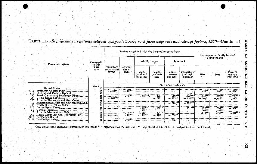
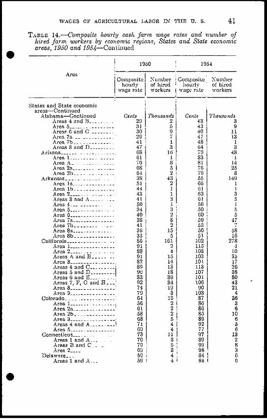
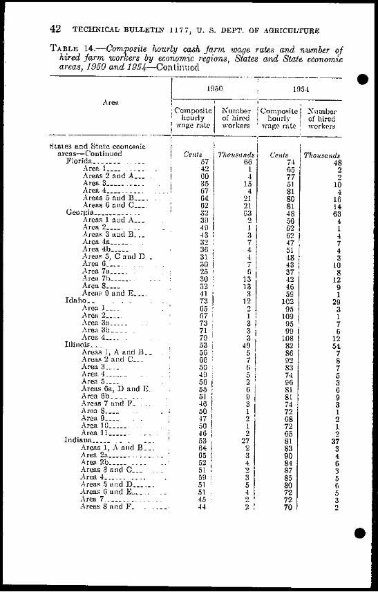

bull
t I