Area Coverage with Unmanned Aerial Vehicles

Using Reinforcement Learning

Research Report

By

Charles Zhang

25 May - 31 July, 2020

Contents

Abstract 2

1 Introduction 2

2 Implementation of Hexagonal Tessellation 2

3 Single Agent Area Coverage 33.1 Overview . . . . . . . . . . . . . . . . . . . . . . . . . . . . . . . . . . . . . . . . . . . . . . . . . . . . 33.2 NMDP Tabular Q Learning . . . . . . . . . . . . . . . . . . . . . . . . . . . . . . . . . . . . . . . . . . 33.3 Graph Based MDP Q Learning . . . . . . . . . . . . . . . . . . . . . . . . . . . . . . . . . . . . . . . . 5

4 Dual Agents Area Coverage 84.1 Overview . . . . . . . . . . . . . . . . . . . . . . . . . . . . . . . . . . . . . . . . . . . . . . . . . . . . 84.2 Multi-Agents Q Learning . . . . . . . . . . . . . . . . . . . . . . . . . . . . . . . . . . . . . . . . . . . 84.3 Actor Critic using Kronecker-Factored Trust Region(ACKTR) . . . . . . . . . . . . . . . . . . . . . . 10

5 Conclusion and Future Work 12

Acknowledgement 12

References 13

1

Abstract

In this summer research, I work with professor Esra Kadioglu-Urtis, and students Aaron Gould, Elisabeth Land-gren, and Fan Zhang at Macalester College. In this project, we first implement the hexagonal tessellation areacoverage approach which Esra previously published. Secondly, we develop and implement Q learning reinforce-ment learning algorithms in a non-Markov Decision Process(NMDP) and Markov Decision Process(MDP) for thearea coverage where, instead of mathematically generating a route, the drone itself will learn an efficient path tocover an entire given area and return back to its launch position. We successfully generate the shortest paths thatcover a large regular or irregular field in terms of the limited drone’s battery life, and finally extend the problemto include multiple drones to considerably widen the coverage area, using the Q learning and Actor Critic usingKronecker-Factored Trust Region (ACKTR) deep reinforcement learning method, built in the Gym environmentin Python or by graph. My code is available at https://github.com/zcczhang/UAV Coverage.

1 Introduction

The coverage path planning(CPP) for Unmanned Aerial Vehicles (a.k.a drones) are increasingly being used formany applications such as search/rescue, agriculture, package delivery, inspection, etc.[1][2][3]. Using UAVs for thecoverage provides several benefits, and UAVs with a high degree of mobility needs to cooperatively work as a teamto provide effective coverage in a relative large are, in consideration of the limited battery life for drones[4].

Many existed work have already addressed the coverage problem by both theoretically methods or learning-based algorithms[5][6][7]. However, drones in those methods are either static for coverage in terms of drones’ fieldof view(FOV), or only complete one-way coverage paths where the cost for the drones’ recovery is not under theconsideration. Therefore, in this work, we not only consider how to generate the shortest coverage paths, but alsoinclude letting the UAV return back to the launch position, which will be addressed in this work using reinforcementlearning algorithms illustrated in detail in the overview sections in this report.

The main contribution of this work is to demonstrate approaches to the reinforcement learning algorithms,named Q-learning and Actor Critic using Kronecker-Factored Trust Region (ACKTR) deep reinforcement learning,to perform the CPP of an regular or irregular environment with known obstacles, visiting only once each center ofthe FOV and returning(for single drone so far), resulting in an optimized path.

2 Implementation of Hexagonal Tessellation

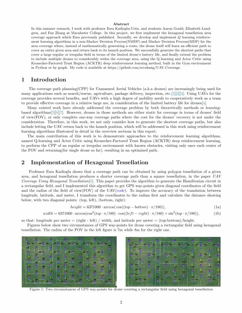
Professor Esra Kadioglu shows that a coverage path can be obtained by using polygon tessellation of a givenarea, and hexagonal tessellation produces a shorter coverage path than a square tessellation, in the paper UAVCoverage Using Hexagonal Tessellation[6]. This paper provides the algorithm to generate the Hamiltonian circuit ina rectangular field, and I implemented this algorithm to get GPS way-points given diagonal coordinates of the fieldand the radius of the field of view(FOV) of the UAV(code). To improve the accuracy of the translation betweenlongitude, latitude, and meter, I transform the coordinates to the radian first and calculate the distance showingbelow, with two diagonal points: (top, left), (bottom, right):

height = 6371000 · arccos( cos((top− bottom) · π/180)), (1a)

width = 6371000 · arccos(cos2(top · π/180) · cos((left− right) · π/180) + sin2(top · π/180)), (1b)

so that: longitude per meter = (right - left) / width, and latitude per meter = (top-bottom)/height.Figures below show two circumstances of GPS way-points for drone covering a rectangular field using hexagonal

tessellation. The radius of the FOV in the left figure is 7m while 8m for the right one.

Figure 1: Two circumstances of GPS way-points for drone covering a rectangular field using hexagonal tessellation

2

3 Single Agent Area Coverage

3.1 Overview

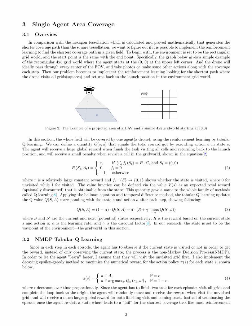
In comparison with the hexagon tessellation which is calculated and proved mathematically that generates theshorter coverage path than the square tessellation, we want to figure out if it is possible to implement the reinforcementlearning to find the shortest coverage path in a given field. To begin with, the environment is set to be the rectangulargrid world, and the start point is the same with the end point. Specifically, the graph below gives a simple exampleof the rectangular 4x5 grid world where the agent starts at the (0, 0) at the upper left corner. And the drone willideally pass through every center of the FOV, and take photos or make some other actions along with the coverageeach step. Then our problem becomes to implement the reinforcement learning looking for the shortest path wherethe drone visits all grids(squares) and returns back to the launch position in the environment grid world.

Figure 2: The example of a projected area of a UAV and a simple 4x5 gridworld starting at (0,0)

In this section, the whole field will be covered by one agent(a drone), using the reinforcement learning by tabularQ learning. We can define a quantity Q(s, a) that equals the total reward got by executing action a in state s.The agent will receive a huge global reward when finish the task visiting all cells and returning back to the launchposition, and will receive a small penalty when revisit a cell in the gridworld, shown in the equation(2).

R (St, At) =

r, if∑i fi (St) = R · C, and St = (0, 0)

0, fi = 0−1, otherwise

(2)

where r is a relatively large constant reward and fi : {S} → {0, 1} shows whether the state is visited, where 0 forunvisited while 1 for visited. The value function can be defined via the value V (s) as an expected total reward(optionally discounted) that is obtainable from the state. This quantity gave a name to the whole family of methodscalled Q-learning[8]. Applying the bellman equation and temporal difference method, the tabular Q learning updatesthe Q value Q(S,A) corresponding with the state s and action a after each step, showing following:

Q(S,A) = (1− α) ·Q(S,A) + α · (R+ γ ·maxa

Q(S′, a)) (3)

where S and S′ are the current and next (potential) states respectively; R is the reward based on the current states and action a; α is the learning rate; and γ is the discount factor[8]. In our research, the state is set to be thewaypoint of the environment—the gridworld in this section.

3.2 NMDP Tabular Q Learning

Since in each step in each episode, the agent has to observe if the current state is visited or not in order to getthe reward, instead of only observing the current state, the process is the non-Markov Decision Process(NMDP).In order to let the agent ”learn” faster, I assume that they will visit the unvisited grid first. I also implement thedecaying epsilon-greedy method to maximize the numerical reward for the action policy π(s) for each state s, shownbelow,

π(s) =

{a ∈ A, P = εa ∈ arg maxa′Qk (sk, a′) , P = 1− ε (4)

where ε decreases over time proportionally. Since the agent has to finish two task for each episode: visit all grids andcomplete the loop back to the origin, the agent will randomly move and receive the reward when visit the unvisitedgrid, and will receive a much larger global reward for both finishing visit and coming back. Instead of terminating theepisode once the agent re-visit a state where leads to a ”fail” for the shortest coverage task like most reinforcement

3

learning algorithms, my algorithm allows the repetition of visits but the agent will receive a negative reward for thepenalty, in order to make the agent ”learn” and distinguish faster both from the good decisions and bad decisions[9].The algorithm below shows the tabular Q learning for one agent looking for the optimal path.

Algorithm 1 NMDP Tabular Q Learning for Area Coverage

1: Initialize the environment R× C board2: Initialize state space S = {(0, 0), . . . , (ROWS − 1, COLS − 1)}3: Initialize action space A = {′up′,′ down′,′ left′,′ right′}, prefer to visit unvisited

grid first4: Reward function R : S ×A → R5: Initialize Q table Q : S ×A → R arbitrarily6: while not reach the number of episodes do7: S ← random S ∈ S8: while not reach END and not visit all do9: set S as visited

10: choose A ∈ A using policy π(S) [4]11: take A, observe S′ whether it is visited, and get R12: Q(S,A)← (1− α) ·Q(S,A) + α · (R+ γ ·maxaQ(S′, a))13: S ← S′

14: decay ε proportionally15: end16: end

where S and S′ are the current and next states respectively; R is the reward based on the action a referring to S,which is dependant on whether the agent visit unvisited states, and finish the coverage task as well as flying back; αis the learning rate; and γ is the discount factor.

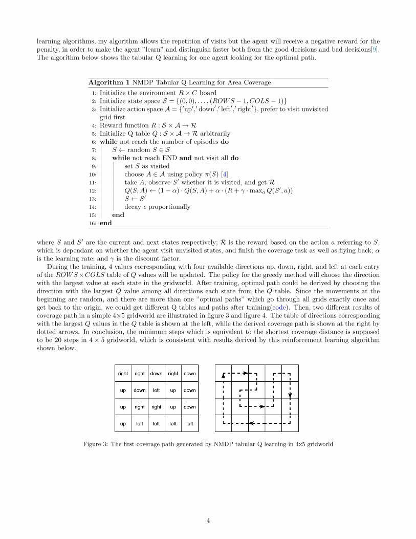
During the training, 4 values corresponding with four available directions up, down, right, and left at each entryof the ROWS×COLS table of Q values will be updated. The policy for the greedy method will choose the directionwith the largest value at each state in the gridworld. After training, optimal path could be derived by choosing thedirection with the largest Q value among all directions each state from the Q table. Since the movements at thebeginning are random, and there are more than one ”optimal paths” which go through all grids exactly once andget back to the origin, we could get different Q tables and paths after training(code). Then, two different results ofcoverage path in a simple 4×5 gridworld are illustrated in figure 3 and figure 4. The table of directions correspondingwith the largest Q values in the Q table is shown at the left, while the derived coverage path is shown at the right bydotted arrows. In conclusion, the minimum steps which is equivalent to the shortest coverage distance is supposedto be 20 steps in 4 × 5 gridworld, which is consistent with results derived by this reinforcement learning algorithmshown below.

Figure 3: The first coverage path generated by NMDP tabular Q learning in 4x5 gridworld

4

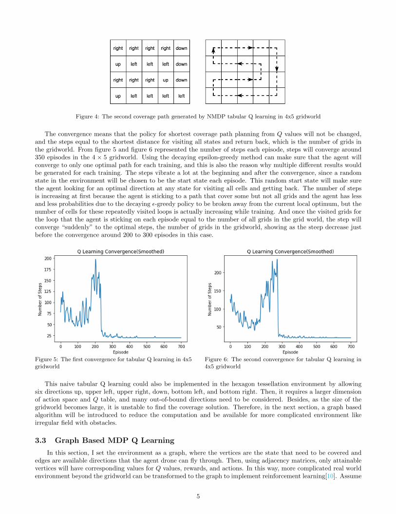
Figure 4: The second coverage path generated by NMDP tabular Q learning in 4x5 gridworld

The convergence means that the policy for shortest coverage path planning from Q values will not be changed,and the steps equal to the shortest distance for visiting all states and return back, which is the number of grids inthe gridworld. From figure 5 and figure 6 represented the number of steps each episode, steps will converge around350 episodes in the 4 × 5 gridworld. Using the decaying epsilon-greedy method can make sure that the agent willconverge to only one optimal path for each training, and this is also the reason why multiple different results wouldbe generated for each training. The steps vibrate a lot at the beginning and after the convergence, since a randomstate in the environment will be chosen to be the start state each episode. This random start state will make surethe agent looking for an optimal direction at any state for visiting all cells and getting back. The number of stepsis increasing at first because the agent is sticking to a path that cover some but not all grids and the agent has lessand less probabilities due to the decaying ε-greedy policy to be broken away from the current local optimum, but thenumber of cells for these repeatedly visited loops is actually increasing while training. And once the visited grids forthe loop that the agent is sticking on each episode equal to the number of all grids in the grid world, the step willconverge “suddenly” to the optimal steps, the number of grids in the gridworld, showing as the steep decrease justbefore the convergence around 200 to 300 episodes in this case.

Figure 5: The first convergence for tabular Q learning in 4x5gridworld

Figure 6: The second convergence for tabular Q learning in4x5 gridworld

This naive tabular Q learning could also be implemented in the hexagon tessellation environment by allowingsix directions up, upper left, upper right, down, bottom left, and bottom right. Then, it requires a larger dimensionof action space and Q table, and many out-of-bound directions need to be considered. Besides, as the size of thegridworld becomes large, it is unstable to find the coverage solution. Therefore, in the next section, a graph basedalgorithm will be introduced to reduce the computation and be available for more complicated environment likeirregular field with obstacles.

3.3 Graph Based MDP Q Learning

In this section, I set the environment as a graph, where the vertices are the state that need to be covered andedges are available directions that the agent drone can fly through. Then, using adjacency matrices, only attainablevertices will have corresponding values for Q values, rewards, and actions. In this way, more complicated real worldenvironment beyond the gridworld can be transformed to the graph to implement reinforcement learning[10]. Assume

5

the environment has V vertices, then R and Q are V × V matrices. Specifically, R is an adjacency matrix exceptR[i, j] where j is the end(start) state and i, j are connected. In this way, each step of exploration will get a smallreward except reaching the end state with a much larger reward. Unlike the NMDP naive Q learning in the previoussection, the agent will first find shortest paths from any state in the environment to the launch position, and thenstore the Q values in Q matrix. This process is MDP, and is straightforward to implement the Q learning. As actionsfor the agent in this MDP are fully random without greedy move, the simple bellman equation is better to use toupdate Q values recursively[11].

Q(S, a) = R(S, a) + α ·maxa

Q(S′, a′) (5)

To get the solution for coverage path planning, I consider that if the agent is supposed to to cover all grids, orin other words visit more states, it is equivalent to avoid the shortest path and minimize the overlapping states, bychoosing the minimum Q value for the policy. The algorithm of this Q learning with graph-based state representationis shown below,

Algorithm 2 Graph-Based State Q Learning for Area Coverage

1: Initialize state space S = {1, . . . , V }2: Initialize action space and reward matrix R: R[S, a], ∀S, a3: Initialize Q table Q: Q[S, a] = null, ∀S, a4: while not reach the number of episodes do5: S ← random S ∈ S6: while S 6= END do7: a← random a valid in the S8: S′ ← a9: Q[S, a]← R[S, a] + α ·maxaQ[S′, a′]

10: S ← S′

11: end12: end13: S = START14: Path is an empty list for the shortest path15: while length(Path) < V do16: add S to Path17: S′ ← S18: S ← argmin(Q[S, ])19: Q[S′, ]← null20: Q[ , S′]← null21: end

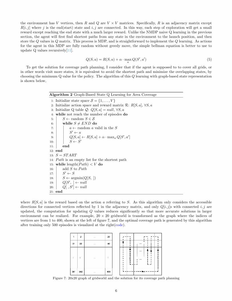
where R[S, a] is the reward based on the action a referring to S. As this algorithm only considers the accessibledirections for connected vertices reflected by 1 in the adjacency matrix, and only Q[i, j]s with connected i, j areupdated, the computation for updating Q values reduces significantly so that more accurate solutions in largerenvironment can be realized. For example, 20 × 20 gridworld is transformed as the graph where the indices ofvertices are from 1 to 400, shown at the left of figure 7, and the optimal coverage path is generated by this algorithmafter training only 500 episodes is visualized at the right(code).

Figure 7: 20x20 graph of gridworld and the solution for its coverage path planning

6

The pattern of the output path for the other sizes of gridworld generated by algorithm 2 are all supposed to bethe zigzag path, similar with 20× 20 gridworld visualized above. It is perspicuous to prove that this is the shortestcoverage path as well as Hamiltonian cycle for the squared tessellation in the gridworld: the shortest coverage pathis the number of vertices times the distance between two centers of two adjacent squares, which is consistent withthe zigzag coverage path generated by Q Learning with Graph-Based State Representations.

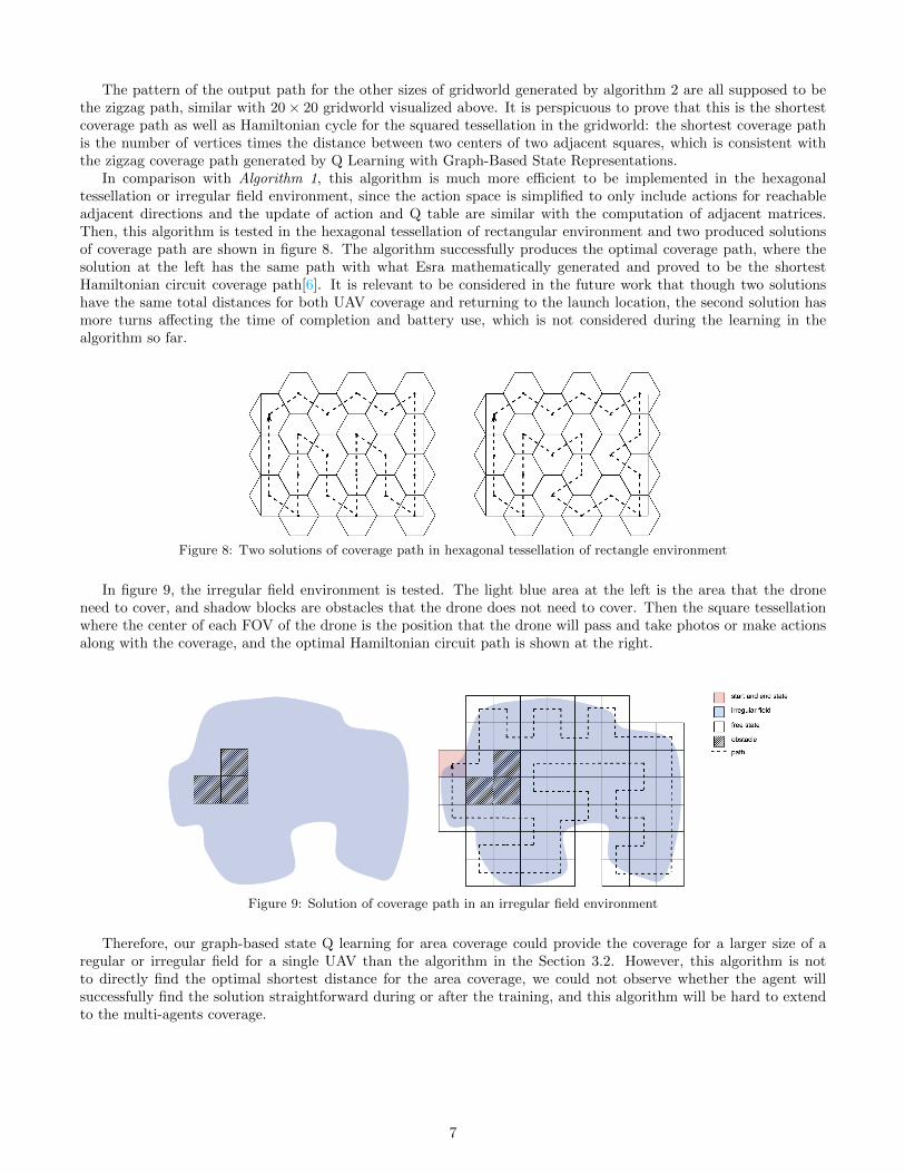
In comparison with Algorithm 1, this algorithm is much more efficient to be implemented in the hexagonaltessellation or irregular field environment, since the action space is simplified to only include actions for reachableadjacent directions and the update of action and Q table are similar with the computation of adjacent matrices.Then, this algorithm is tested in the hexagonal tessellation of rectangular environment and two produced solutionsof coverage path are shown in figure 8. The algorithm successfully produces the optimal coverage path, where thesolution at the left has the same path with what Esra mathematically generated and proved to be the shortestHamiltonian circuit coverage path[6]. It is relevant to be considered in the future work that though two solutionshave the same total distances for both UAV coverage and returning to the launch location, the second solution hasmore turns affecting the time of completion and battery use, which is not considered during the learning in thealgorithm so far.

Figure 8: Two solutions of coverage path in hexagonal tessellation of rectangle environment

In figure 9, the irregular field environment is tested. The light blue area at the left is the area that the droneneed to cover, and shadow blocks are obstacles that the drone does not need to cover. Then the square tessellationwhere the center of each FOV of the drone is the position that the drone will pass and take photos or make actionsalong with the coverage, and the optimal Hamiltonian circuit path is shown at the right.

Figure 9: Solution of coverage path in an irregular field environment

Therefore, our graph-based state Q learning for area coverage could provide the coverage for a larger size of aregular or irregular field for a single UAV than the algorithm in the Section 3.2. However, this algorithm is notto directly find the optimal shortest distance for the area coverage, we could not observe whether the agent willsuccessfully find the solution straightforward during or after the training, and this algorithm will be hard to extendto the multi-agents coverage.

7

4 Dual Agents Area Coverage

4.1 Overview

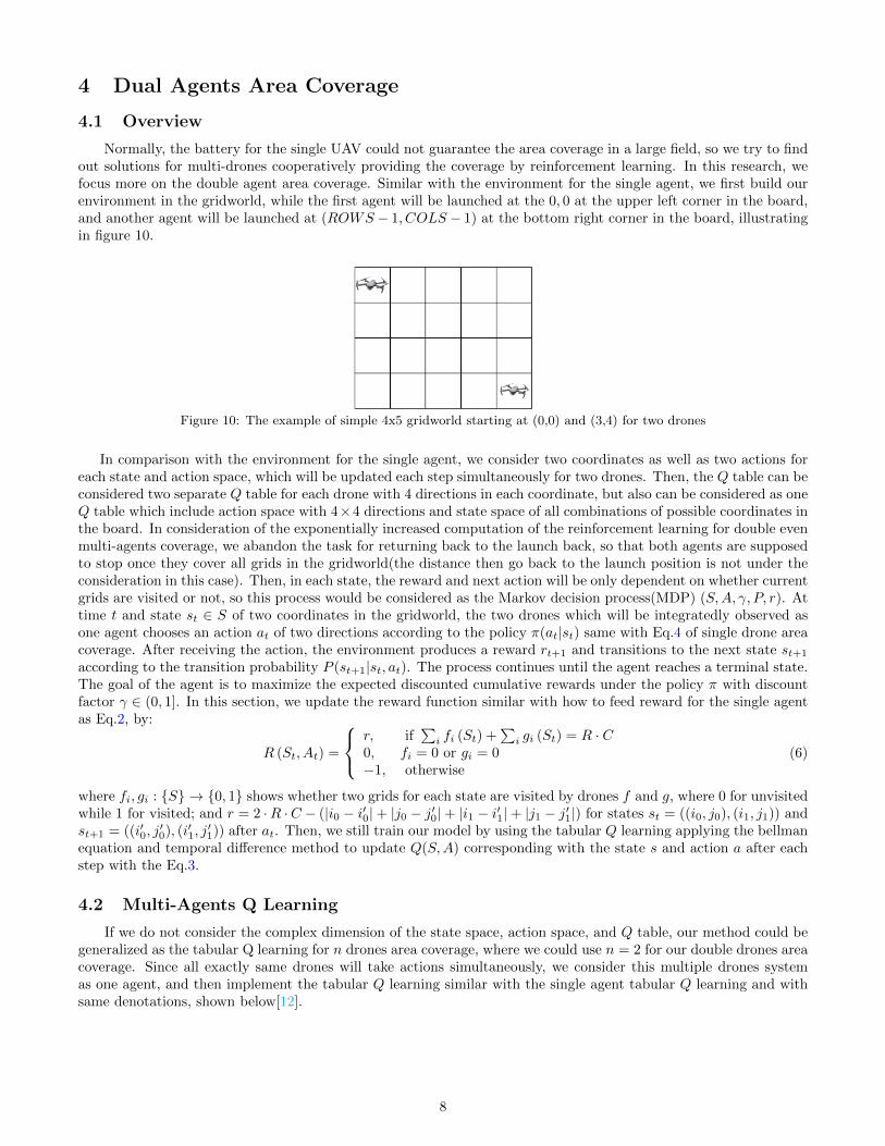
Normally, the battery for the single UAV could not guarantee the area coverage in a large field, so we try to findout solutions for multi-drones cooperatively providing the coverage by reinforcement learning. In this research, wefocus more on the double agent area coverage. Similar with the environment for the single agent, we first build ourenvironment in the gridworld, while the first agent will be launched at the 0, 0 at the upper left corner in the board,and another agent will be launched at (ROWS − 1, COLS − 1) at the bottom right corner in the board, illustratingin figure 10.

Figure 10: The example of simple 4x5 gridworld starting at (0,0) and (3,4) for two drones

In comparison with the environment for the single agent, we consider two coordinates as well as two actions foreach state and action space, which will be updated each step simultaneously for two drones. Then, the Q table can beconsidered two separate Q table for each drone with 4 directions in each coordinate, but also can be considered as oneQ table which include action space with 4×4 directions and state space of all combinations of possible coordinates inthe board. In consideration of the exponentially increased computation of the reinforcement learning for double evenmulti-agents coverage, we abandon the task for returning back to the launch back, so that both agents are supposedto stop once they cover all grids in the gridworld(the distance then go back to the launch position is not under theconsideration in this case). Then, in each state, the reward and next action will be only dependent on whether currentgrids are visited or not, so this process would be considered as the Markov decision process(MDP) (S,A, γ, P, r). Attime t and state st ∈ S of two coordinates in the gridworld, the two drones which will be integratedly observed asone agent chooses an action at of two directions according to the policy π(at|st) same with Eq.4 of single drone areacoverage. After receiving the action, the environment produces a reward rt+1 and transitions to the next state st+1

according to the transition probability P (st+1|st, at). The process continues until the agent reaches a terminal state.The goal of the agent is to maximize the expected discounted cumulative rewards under the policy π with discountfactor γ ∈ (0, 1]. In this section, we update the reward function similar with how to feed reward for the single agentas Eq.2, by:

R (St, At) =

r, if∑i fi (St) +

∑i gi (St) = R · C

0, fi = 0 or gi = 0−1, otherwise

(6)

where fi, gi : {S} → {0, 1} shows whether two grids for each state are visited by drones f and g, where 0 for unvisitedwhile 1 for visited; and r = 2 ·R ·C − (|i0 − i′0|+ |j0 − j′0|+ |i1 − i′1|+ |j1 − j′1|) for states st = ((i0, j0), (i1, j1)) andst+1 = ((i′0, j

′0), (i′1, j

′1)) after at. Then, we still train our model by using the tabular Q learning applying the bellman

equation and temporal difference method to update Q(S,A) corresponding with the state s and action a after eachstep with the Eq.3.

4.2 Multi-Agents Q Learning

If we do not consider the complex dimension of the state space, action space, and Q table, our method could begeneralized as the tabular Q learning for n drones area coverage, where we could use n = 2 for our double drones areacoverage. Since all exactly same drones will take actions simultaneously, we consider this multiple drones systemas one agent, and then implement the tabular Q learning similar with the single agent tabular Q learning and withsame denotations, shown below[12].

8

Algorithm 3 Multi-Drones tabular Q Learning for Area Coverage

1: Initialize the environment R× C board and n agents2: Initialize S = (s0, s1, ..., sn), si ∈ {(0, 0), . . . , (R− 1, C − 1)}, 0 ≤ i ≤ n3: Initialize A = (a0, a1, ..., an), ai ∈ {′up′,′ down′,′ left′,′ right′}, 0 ≤ i ≤ n4: Reward function R : S ×A → R5: Initialize Q table Q : S ×A → R arbitrarily6: while not reach the number of episodes do7: reset S = (s0, s1, ..., sn) to their initial positions8: while not cover all in board do9: set s0, s1, ..., sn in S as visited in board

10: choose A = (a0, a1, ..., an) using policy [4] for each ai, 0 ≤ i ≤ n11: S′ = (s′0, s

′1, ..., s

′n)

12: observe s′i, 0 ≤ i ≤ n whether it is visited, and get R13: Q(S,A)← (1− α) ·Q(S,A) + α · (R+ γ ·maxaQ(S′, a))14: S ← S′

15: end16: end

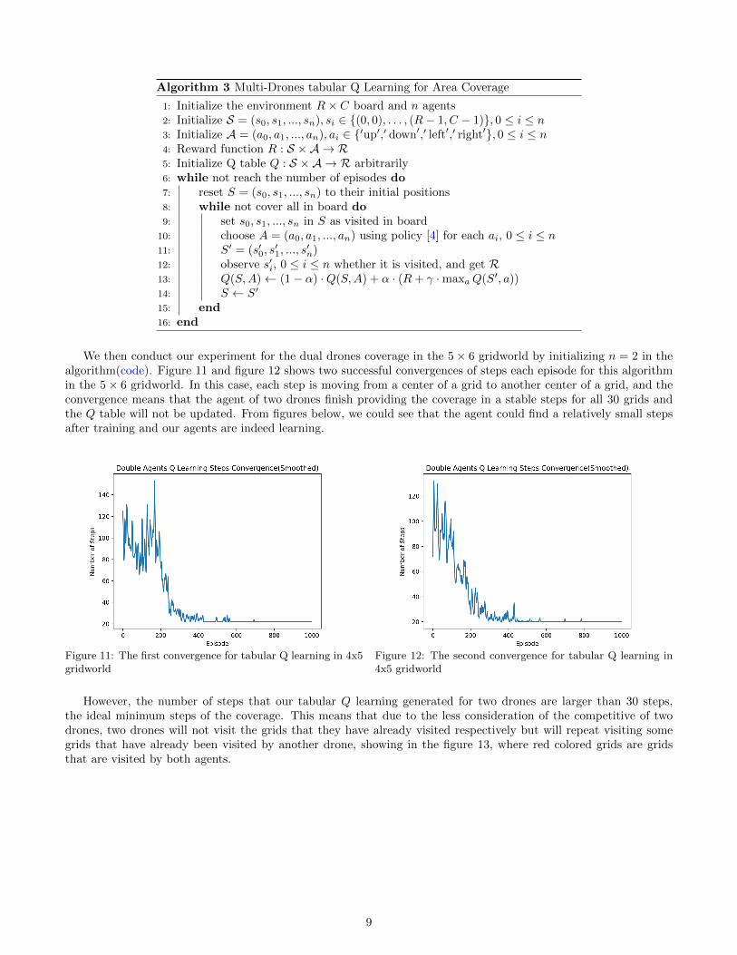
We then conduct our experiment for the dual drones coverage in the 5× 6 gridworld by initializing n = 2 in thealgorithm(code). Figure 11 and figure 12 shows two successful convergences of steps each episode for this algorithmin the 5× 6 gridworld. In this case, each step is moving from a center of a grid to another center of a grid, and theconvergence means that the agent of two drones finish providing the coverage in a stable steps for all 30 grids andthe Q table will not be updated. From figures below, we could see that the agent could find a relatively small stepsafter training and our agents are indeed learning.

Figure 11: The first convergence for tabular Q learning in 4x5gridworld

Figure 12: The second convergence for tabular Q learning in4x5 gridworld

However, the number of steps that our tabular Q learning generated for two drones are larger than 30 steps,the ideal minimum steps of the coverage. This means that due to the less consideration of the competitive of twodrones, two drones will not visit the grids that they have already visited respectively but will repeat visiting somegrids that have already been visited by another drone, showing in the figure 13, where red colored grids are gridsthat are visited by both agents.

9

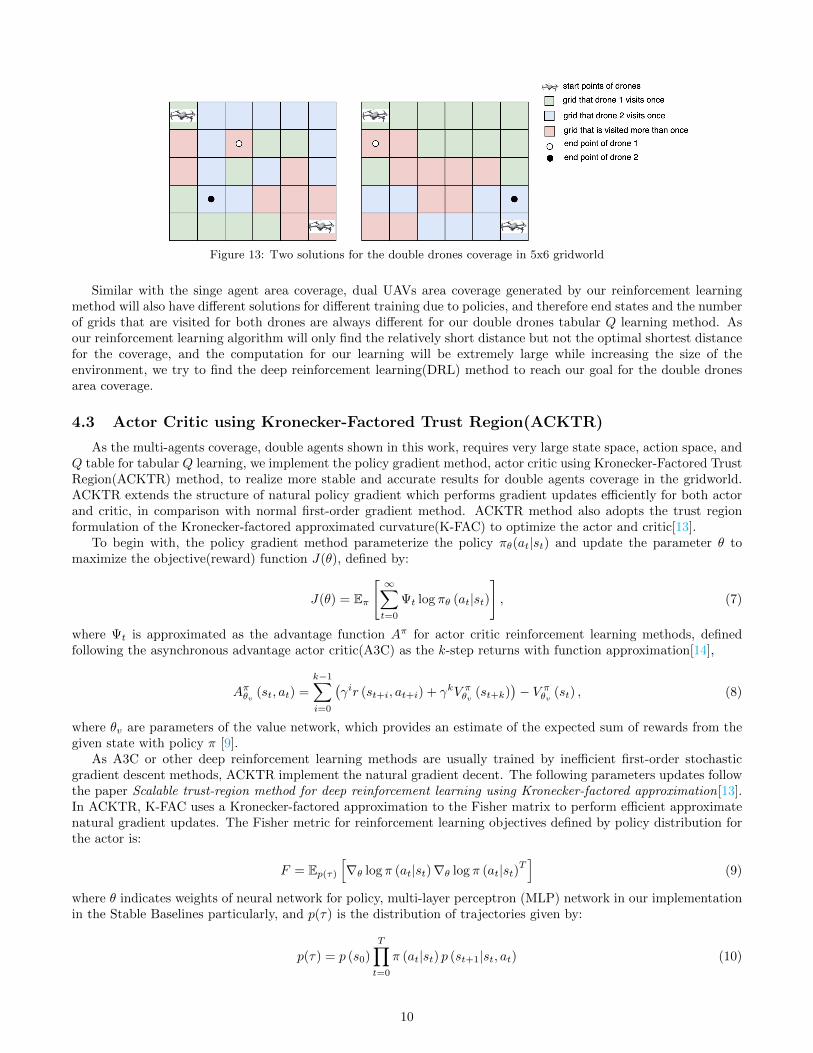
Figure 13: Two solutions for the double drones coverage in 5x6 gridworld

Similar with the singe agent area coverage, dual UAVs area coverage generated by our reinforcement learningmethod will also have different solutions for different training due to policies, and therefore end states and the numberof grids that are visited for both drones are always different for our double drones tabular Q learning method. Asour reinforcement learning algorithm will only find the relatively short distance but not the optimal shortest distancefor the coverage, and the computation for our learning will be extremely large while increasing the size of theenvironment, we try to find the deep reinforcement learning(DRL) method to reach our goal for the double dronesarea coverage.

4.3 Actor Critic using Kronecker-Factored Trust Region(ACKTR)

As the multi-agents coverage, double agents shown in this work, requires very large state space, action space, andQ table for tabular Q learning, we implement the policy gradient method, actor critic using Kronecker-Factored TrustRegion(ACKTR) method, to realize more stable and accurate results for double agents coverage in the gridworld.ACKTR extends the structure of natural policy gradient which performs gradient updates efficiently for both actorand critic, in comparison with normal first-order gradient method. ACKTR method also adopts the trust regionformulation of the Kronecker-factored approximated curvature(K-FAC) to optimize the actor and critic[13].

To begin with, the policy gradient method parameterize the policy πθ(at|st) and update the parameter θ tomaximize the objective(reward) function J(θ), defined by:

J(θ) = Eπ

[ ∞∑t=0

Ψt log πθ (at|st)

], (7)

where Ψt is approximated as the advantage function Aπ for actor critic reinforcement learning methods, definedfollowing the asynchronous advantage actor critic(A3C) as the k-step returns with function approximation[14],

Aπθv (st, at) =

k−1∑i=0

(γir (st+i, at+i) + γkV πθv (st+k)

)− V πθv (st) , (8)

where θv are parameters of the value network, which provides an estimate of the expected sum of rewards from thegiven state with policy π [9].

As A3C or other deep reinforcement learning methods are usually trained by inefficient first-order stochasticgradient descent methods, ACKTR implement the natural gradient decent. The following parameters updates followthe paper Scalable trust-region method for deep reinforcement learning using Kronecker-factored approximation[13].In ACKTR, K-FAC uses a Kronecker-factored approximation to the Fisher matrix to perform efficient approximatenatural gradient updates. The Fisher metric for reinforcement learning objectives defined by policy distribution forthe actor is:

F = Ep(τ)[∇θ log π (at|st)∇θ log π (at|st)T

](9)

where θ indicates weights of neural network for policy, multi-layer perceptron (MLP) network in our implementationin the Stable Baselines particularly, and p(τ) is the distribution of trajectories given by:

p(τ) = p (s0)

T∏t=0

π (at|st) p (st+1|st, at) (10)

10

As in ACKTR the output of the critic v is defined to be a Gaussian distribution as p(a, v|s) = π(a|s)p(v|s), andwhen actor and critic share lower-layer representations, ACKTR applies K-FAC to approximate the Fisher matrixto perform updates simultaneously.

F = Ep(τ)[∇θ log p(a, v|s)∇θ log p(a, v|s)T

](11)

Then, ACKTR applies trust region formulation of K-FAC, with the following updates of effective step size η forthe natural gradient:

η = min(ηmax,

√2δ

∆θTF̂∆θ) (12a)

θ ← θ − ηF−1∇θL (12b)

where ηmax is the learning rate and δ is the trust region radius. ACKTR is the first scalable trust region naturalgradient method for actor-critic DRL, and improves the sample efficiency of current methods significantly[13]. Wewill use this method to train our agents for the double agents coverage in the gridworld. We conduct our experimentfor double UAVs coverage in a 10× 10 gridworld, where the start positions for drones are the upper left and bottomright of the board respectively, and the end points are undecided to make sure that the training process is MDP. Wesuccessfully find solutions for double agents area coverage using ACKTR(code). Figure 14 shows two solutions forthe coverage path planning after training 200,000 time-steps, using ACKTR implemented in the Stable Baselines inPython(simulation code).

Figure 14: solutions for double agents coverage path planning in 10x10 gridworld

Figure 15 and 16 below represent the learning curve indicating the rewards the agent received each episode. Therewards received each episode are increasing overall and become stable around 70 after 150,000 time-steps. Thereward feeding are typically follows Eq.6, and figure 15 and 16 illustrate how ACKTR method maximize the rewardsby updating parameters of layers each time-step while training. Two figures below are learning curves indicatingrewards for solutions illustrated in figure 14. The rewards are showing increasing overall and becoming stable afteraround 150,000 time-steps. Therefore, we could conclude that it is realizable to use ACKTR deep reinforcementlearning method to complete the area coverage path planning for two agents.

11

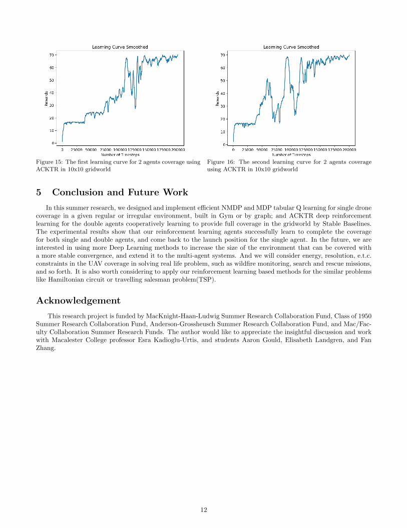
Figure 15: The first learning curve for 2 agents coverage usingACKTR in 10x10 gridworld

Figure 16: The second learning curve for 2 agents coverageusing ACKTR in 10x10 gridworld

5 Conclusion and Future Work

In this summer research, we designed and implement efficient NMDP and MDP tabular Q learning for single dronecoverage in a given regular or irregular environment, built in Gym or by graph; and ACKTR deep reinforcementlearning for the double agents cooperatively learning to provide full coverage in the gridworld by Stable Baselines.The experimental results show that our reinforcement learning agents successfully learn to complete the coveragefor both single and double agents, and come back to the launch position for the single agent. In the future, we areinterested in using more Deep Learning methods to increase the size of the environment that can be covered witha more stable convergence, and extend it to the multi-agent systems. And we will consider energy, resolution, e.t.c.constraints in the UAV coverage in solving real life problem, such as wildfire monitoring, search and rescue missions,and so forth. It is also worth considering to apply our reinforcement learning based methods for the similar problemslike Hamiltonian circuit or travelling salesman problem(TSP).

Acknowledgement

This research project is funded by MacKnight-Haan-Ludwig Summer Research Collaboration Fund, Class of 1950Summer Research Collaboration Fund, Anderson-Grossheusch Summer Research Collaboration Fund, and Mac/Fac-ulty Collaboration Summer Research Funds. The author would like to appreciate the insightful discussion and workwith Macalester College professor Esra Kadioglu-Urtis, and students Aaron Gould, Elisabeth Landgren, and FanZhang.

12

References

[1] E. Semsch, M. Jakob, D. P. ıcek, and M. Pechoucek, “Autonomous uav surveillance in complex urban environ-ments,” Proceedings of the 2009 IEEE/WIC/ACM International Conference on Intelligent Agent Technology,IAT 2009, Milan, Italy, 15-18, 2009.

[2] M. Silvagni, A. Tonoli, E. Zenerino, and M. Chiaberg, “Multipurpose uav for search and rescue operations inmountain avalanche events,” Geomatics, Natural Hazards and Risk, pp. 1–16, 2016.

[3] T. Oksanen and A. Visala, “Coverage path planning algorithms for agricultural field machines,” J. Field Robotics,vol. 26, pp. 651–668, 2009.

[4] Liu, C. Harold, Z. Chen, J. Tang, J. Xu, and C. Piao., “Energy-efficient uav control for effective and faircommunication coverage: A deep reinforcement learning approach,” IEEE Journal on Selected Areas in Com-munications 36, no. 9, 2018.

[5] T. M. Cabreira, L. B. Brisolara, and P. R. F. Jr, “Esurvey on coverage path planning with unmanned aerialvehicles,” Drones, 3(1), 4., 2019.

[6] E. Kadioglu, C. Urtis, and N. Papanikolopoulos, “UAV Coverage Using Hexagonal Tessellation,” 2019 27th

Mediterranean Conference on Control and Automation (MED), IEEE, 2019.

[7] Panov, A. I., K. S. Yakovlev, and R. Suvorov, “Grid path planning with deep reinforcement learning: Preliminaryresults,” Procedia computer science 123, 2018.

[8] Lapan and Maxim, Deep Q-Networks. Deep Reinforcement Learning Hands-On: Apply modern RL methods,with deep Q-networks, value iteration, policy gradients, TRPO, AlphaGo Zero and more. Chapter 6. Page 130.Packt Publishing Ltd, 2018.

[9] R. S. Sutton and A. G. Barto, Reinforcement learning: An introduction. MIT press, 2018.

[10] Piardi, Luis, J. Lima, A. I. Pereira, and P. Costa, “Coverage path planning optimization based on q-learningalgorithm,” AIP Conference Proceedings. Vol. 2116. No. 1. AIP Publishing LLC, 2019.

[11] Lapan and Maxim, Tabular Learning and the Bellman Equation. Deep Reinforcement Learning Hands-On: Applymodern RL methods, with deep Q-networks, value iteration, policy gradients, TRPO, AlphaGo Zero and more.Chapter 5. Page 113. Packt Publishing Ltd, 2018.

[12] PGreenwald, Amy, K. Hall, and R. Serrano, “Correlated q-learning,” ICML. Vol. 20. No. 1, 2003.

[13] Y. Wu, E. Mansimov, R. B. Grosse, S. Liao, and J. Ba, “Scalable trust-region method for deep reinforcementlearning using kronecker-factored approximation,” In Advances in neural information processing systems, pp.5279-5288, 2017.

[14] Mnih, Volodymyr, A. P. Badia, M. Mirza, A. Graves, T. Lillicrap, T. Harley, D. Silver, and K. Kavukcuoglu,“Asynchronous methods for deep reinforcement learning.,” International conference on machine learning. pp.1928-1937, 2016.

13