Are Environmentally Related Taxes Effective?

Sebastián J. Miller Mauricio A. Vela

Department of Research and Chief Economist

IDB-WP-467IDB WORKING PAPER SERIES No.

Inter-American Development Bank

November 2013

Are Environmentally Related Taxes Effective?

Sebastián J. Miller Mauricio A. Vela

Inter-American Development Bank

2013

Inter-American Development Bank

http://www.iadb.org The opinions expressed in this publication are those of the authors and do not necessarily reflect the views of the Inter-American Development Bank, its Board of Directors, or the countries they represent.

The unauthorized commercial use of Bank documents is prohibited and may be punishable under the

Bank's policies and/or applicable laws.

Copyright © Inter-American Development Bank. This working paper may be reproduced for any non-commercial purpose. It may also be reproduced in any academic journal indexed by the American Economic Association's EconLit, with previous consent by the Inter-American Development Bank (IDB), provided that the IDB is credited and that the author(s) receive no income from the publication.

Cataloging-in-Publication data provided by the Inter-American Development Bank Felipe Herrera Library Miller, Sebastián J. Are Environmentally Related Taxes Effective / Sebastián J. Miller, Mauricio A. Vela. p. cm. — (IDB Working Paper Series ; 467) Includes bibliographical references. 1. Environmental impact charges. 2. Pollution. 3. Environmental quality. 4. Tax revenue estimating. I. Vela, Mauricio A. II. Inter-American Development Bank. Research Dept. III. Title. IV. Series. IDB-WP-467

2013

Are environmentally related taxes effective?

Sebastian J. Miller∗and Mauricio A. Vela†

∗Research Department, Inter-American Development Bank†Research Department, Inter-American Development Bank

Abstract

This paper focuses on the question of whether the magnitude of long-established en-vironmentally related taxes (ERT) is related to countries environmental performance.While environmental taxes efficiencies have previously been discussed, those taxescontribution to reducing pollution and improving environmental quality has not beenfully explored. This paper therefore analyzes the effectiveness of environmental taxesby examining the environmental performance of 50 countries from all regions in asso-ciation with the amount of revenues from environmentally related taxes each countrycollects. Using a cross-section regression and a panel dynamic regression, the paperfinds that countries with higher revenues from these types of taxes also exhibit higherreductions in CO2 emission, PM10 emissions, and energy consumption and produc-tion from fossil sources.

JEL classification: H23, Q58, Q530.Keywords: Environmental Tax; Environmental Policy; Pollution.

1 Introduction

In the economic literature, environmental taxes have been proposed as one of the main instrumentsfor the mitigation of environmental problems such as pollution and climate change (e.g., Pigou ,1920). Such instruments are classified as incentive-based mechanisms, as it is argued that taxescreate the right incentives for agents to refrain from polluting above the socially “accepted level”,internalizing the external costs. They can also be more efficient than so called command-and-control mechanisms, and their administration costs tend to be low (Baumol and Oates , 1988).Pollution is an example of a negative externality that needs to be corrected, and taxes, fees andcharges can induce polluters to internalize the cost of pollution they are imposing on the rest ofsociety.

However, in the real world the debate is much more complicated. It is not easy to achievea socially optimal outcome, and there is not a clear formula to establish the most efficient tax rate(e.g., Parry and Small , 2004, Newberry , 2004). Besides, as different studies have shown, environ-mental taxes may have some negative consequences. Wier et al. (2005), for example, concludesthat environmental taxes in Denmark have undesirable consequences in terms of distributionaleffects, as those taxes are shown to be regressive. Similar results are found by Brannlund andNordstrom (2004), West and Williams III (2004) for Sweden and the United States. These impli-cations enhance the importance of compensatory mechanisms that should come with the adaptationof such measures.

Environmental taxes clearly have political costs that complicate their implementation. Nonethe-less, countries have employed taxes that, despite not being established for environmental reasons,perform similarly to an environmental tax. Some of the best-known and most frequently imple-mented environmentally related taxes (ERTs) are taxes on the use of fossil fuels such as petrol(gasoline) and diesel, the widespread adoption of which is explained by their ability to raise largefiscal revenues. The efficiency and distributional consequences of those taxes have been examinedin many studies. Beyond these considerations, however, environmental taxes have been continuallyconstraining agents in the economy, possibly affecting the consumption of fossil fuels and otherpollution-intensive goods. Relatively few studies have considered the effectiveness of those taxesin this regard.

The rates and number of ERTs varies considerably from country to country. While somecountries may impose higher taxes as part of their environmental policy, others may grant hugesubsidies for fossil fuel consumption or the use of other pollution inputs. These differences maybe easily perceived when comparing levels of ERT revenues. In this paper, revenue from ERTswill be used as a proxy of the level and magnitude of ERTs. The majority of these revenuescome from fuel and transport activities, and these fuel taxes have had the aim of raising revenuerather than reducing fuel use. Although ERTs were not originally established as an environmentalpolicy instrument, they could perform well in dealing with some environmental problems, and it istherefore essential to determine the extent of such side effects.

Studies analyzing the short and long-run demand elasticities of fossil fuels have shown thattheir demand is not very price sensitive. However, in the long run fuel taxes can lead to a negativetime trend in price elasticity, mainly driven by responses in fuel efficiency and mileage per carfor the case of gasoline (Brons et al. , 2008). In this study we will focus on long-run impacts,and our proxy for ERTs may have the advantage of considering the general impact of different taxrates rather than of only one particular tax rate. Therefore, the idea of this work is to shed light

2

on the association between the revenues from environmentally related taxes and the performanceof some environmental variables. This work uses data from the OECD for 50 countries, mainlyOECD countries but also including some countries from Latin America and Eastern Europe, aswell as China and South Africa. The evidence here does not show any causal relationship or provethe efficiency of each environmental tax, but it does suggest that the magnitude and quantity ofthese taxes may affect environmental quality. In other words, countries that differ in revenuesfrom environmental taxes experience different results in pollution abatement and environmentalconservation.

Given global concern about climate change and pollution costs, market-based instrumentsmay have the potential to mitigate those problems. Market-based instruments have been less usedthan command-and-control standards, 1 but some experiences have shown that, with a correctdesign and in the correct circumstances, these instruments can be appropriate for dealing withenvironmental problems.

Section 2 describes some of the literature on environmentally related taxes and their inci-dence. It is followed by Section 3, in which ERTs are defined and explained. This section alsodescribes other variables taken into account. Section 5 shows the benchmark estimations usinga cross-section approach, while Section 6 estimates a dynamic panel model using GMM. Finally,conclusions are presented in Section 7.

2 Literature ReviewOne main branch of the literature on the effects of environmentally related taxes on environmentalperformance focuses on carbon taxes, which are levied on fossil fuels and other products accordingto their carbon content in order to reduce CO2 emissions. For example, Gerlagh and van der Zwaan(2006) use a top-down energy demand model to analyze various instruments including carbon

taxes. The authors find that a portfolio standard for carbon dioxide emission intensity by recyclingcarbon taxes as subsidies to non-fossil energy is the cheapest option for mitigating climate changein comparison to subsidies for non-fossil energy production and to carbon and fossil fuel taxes.

Bruvoll and Larsen (2004), using an applied general equilibrium simulation, analyze theeffect of carbon taxes on emissions change in Norway. They found that carbon taxes had a modesteffect on the reduction of CO2, contributing to a 2% decrease. The reduction in emissions perunit of GDP is significant, however, and the main effect was the reduction on energy intensity andprocess emissions. The main argument shared by some studies is the null effects of environmentaltaxes on CO2 emissions if they are accompanied by tax exemptions on energy-intensive industriesand if they are applied to sectors with high inelastic demands. Liang et al. (2007) arrive at thesame conclusion after using a CGE model to evaluate the impact of different carbon tax scenariosfor China. In a scenario where energy and trade-intensive sectors are fully exempted and whereall un-exempted sectors are subsidized, mitigation effects are very weak and exempted sector CO2emissions rise. On the other hand, in this scenario the negative impacts of carbon taxes on GDP,employment and consumption are reduced, and output and exports in the trade-intensive sector arenot affected.

In a forecast study on the effect of energy and carbon taxes on the energy system in Japan,Nakata and Lamont (2001) support the idea that these taxes are a suitable instrument for reducing

1 typically known as regulations or standards that impose strict restrictions on activity or use of inputs

3

CO2 emissions. Wissema and Dellink (2007) studies the Irish case and finds that a reduction of25% relative to the 1998 level of CO2 can be achieved with a carbon tax of 10 to 15 euros perton of CO2. Di Cosmo and Hyland (2011), also taking into account the Irish case, use differenttax scenarios to look at impacts on energy demand and carbon dioxide emissions. With a scenarioof carbon tax increase from 21.5 euros in 2012 to 41 euros in 2025, the authors find that CO2emissions will be reduced by 861,000 tons relative to a zero carbon tax scenario.

Some experiences with ERTs have been adversely affected by incorrect tax exemptionsand poorly planned refund systems. Vehmas (2005) analyzes the experience of Finland withenvironmentally-based energy taxation and concludes that fiscally motivated deviations from theideal environmental tax have undermined the real purpose of the tax.

Certain authors highlight the importance of fossil fuel taxes. For example, Sterner (2007)show the positive long-run effect of fossil fuel taxes in Europe in terms of reducing fuel demandand reducing carbon emissions. The author explains that carbon emissions are cut more than halfby introducing high fuel taxes and the carbon content of the atmosphere is reduced by more than1 ppm. In the same line, Yan and Crookes (2009) explain the importance of a scenario with fossilfuel taxes in order to deal with the rapid growth of vehicles and energy demand in China. Thisscenario leads to a potential reduction of 16.3% in energy demand, 18.5% in petroleum demandand 16.2% in GHG emissions by 2030 compared to the business as usual scenario.

Concrete empirical evidence has shown the effectiveness of some environmentally relatedtaxes. Convery et al. (2007) underscore the effectiveness of the plastic bag levy in Ireland whichstarted in 2002. One main result is that consumption of plastic bags in retail outlets fall by morethan 90% and the annual revenues from this tax are around 13 million euros. Deyle and Bretschnei-der (1995) analyze waste taxes in United States, in particular taxes on land disposal, and find thathigher taxes reduce wastes sent to landfills in comparison to other form of management.

Other works look at the effect of carbon taxes on emissions. Lin and Li (2011) use a dif-ference in differences approach to analyze the effect of carbon taxes on per capita CO2 emissions.The authors find some significant effect in reducing CO2 emissions in Finland and a negative butnot significant coefficient for the Netherlands, Denmark and Sweden. For Norway the effect wasthe opposite, an increase in CO2 emissions per capita, explained by the growth of energy products.

2.1 HypothesisAs seen above, the introduction of environmental taxes can be effective in controlling pollution.When taxing energy or any pollution-intensive good, firms producing that good will internalize thesocial cost of pollution, which in the before-tax situation did not appear in the final price of thatgood. The price of these goods will thus increase with the tax and, therefore, the production ofthat good will decrease. Additionally, the resources freed up will help increase the production ofenvironmentally friendly goods. Nonetheless, the effect of introducing these types of taxes couldonly be seen in long-term periods. Firms need time to substitute their inputs and production, andhigh demand inelasticity of energy goods will make also the environmental tax less effective inthe short run. For this reason, we will initially consider periods of 15 years in the cross-sectionalresults and periods of at least two years in the dynamic GMM results when analyzing the impactof ERTs on pollution and pollution-intensive goods.

The hypothesis tested here is that countries that establish higher ERTs will have lower lev-els of pollution and less future production and consumption of non-renewable energy. A set of

4

outcome variables for environmental pollution and fossil-related energy production and consump-tion is used. Environmental taxes will trigger agents in an economy to follow a diminishing pathof energy consumption and pollution emission. Therefore, we expect a greater reduction in thesevariables in countries with higher initial ERTs. Initially, we will use the longest available period ofthe dataset, 15 years, by using a cross-sectional regression. To take advantage of the panel structureof the data and have more power for our regressions results, however, we will also use a dynamicsystem GMM to analyze the two or four-year change in our variables of interest. Using a GMMsystem allows us to deal with small sample bias, given that the number of time periods is small,with high persistence of variables.

3 Data Description4 Environmentally Related TaxesEnvironmentally related taxes are defined by the OECD as every payment to the general govern-ment levied on tax bases that have any environmental relevance2. Taxes are unrequited in the sensethat benefits provided by government to taxpayers are not in proportion to their payments. There-fore, this definition takes into account the effect on relevant price elasticity and also implies thatnot every ERT was implemented with a specific environmental goal but does have, at least theoret-ically, a final positive impact on the environment. The main feature of ERTs is consequently thatthey incorporate the cost of pollution into final prices and thus create incentives for producers andconsumers to change their behavior toward less environmental damage. The ERTs data analyzedin this paper were obtained from OECD, Eurostat and IEA3.

Environmentally related taxes have been established in many countries and in differentperiods of time. The early 1990s witnessed increasing interest in environmental policy and theintroduction of many “green” reforms; at that time Nordic countries were among the pioneers inimplementing ERTs with a primarily environmental focus. Of these taxes, taxes on fuels are themost common type and generate the largest amount of revenues. Figure 1 shows that for mostcountries energy taxes are more important than pollution, resource and transport taxes.

2 Value added taxes (VAT) are excluded.3 Information about environmentally related taxes and some data description can be found athttp://www2.oecd.org/ecoinst/queries/

5

Figure 1. Revenue from Environmentally Related Taxes as Percentage of GDP in 2010

0 1 2 3 4Revenue from envrionmentally related tax % of gdp in 2010

ESPISL

FRASVKLTUROUBEL

DEUAUT

IRLLUXCZEGRCLVAPRTITA

POLNORGBR

HUNSWEFIN

BGRCYPEST

MLTSVNNLDDNK

ERT’s − energy taxes ERT’s − transport taxes

ERT’s − pollution/resources taxes

Source: OECD, Eurostats.

The variation in the level and timing of carbon taxes illustrates the overall divergenceamong countries’ ERTs. Finland was the first to introduce a carbon tax in 1990 with a rate of$30 per metric ton of CO2, and Sweden adopted a carbon tax in 1991 with a rate of $105 per met-ric ton of CO2, while in the U.S. state of California a carbon tax was only introduced in 2008, witha rate of only $0.045 per metric ton CO2 (Summer et al. , 2009). It is important to note, however,that environmentally related taxes are not the only environmental instrument used and not alwaysthe most efficient one (O′Ryan et al. , 2003). In fact, this instrument has always been accompaniedby command-and-control policies such as environmental standard regulations.

In this paper, revenues from ERTs as a percentage of GDP will be used as a proxy forERTs. Information from OECD and the Eurostat database of 50 countries is available, mostlyOECD countries but also including some countries of Latin America and Eastern Europe, as wellas China and South Africa. Table A.5 in the Appendix shows all the countries and the average ofsome variables for the period of analysis between 1995 and 2010.

Higher revenues from ERTs will not necessarily be linked to higher tax rates, as a scenariowith high consumption of lightly taxed goods is possible. Additionally, a more effective tax maydiminish the base of the environmental tax, thereby reducing total revenue from ERTs. Neverthe-less, this situation is not common, and countries with higher revenues from ERTs generally havehigher tax rates (OECD , 2006). Most of the revenues from ERTs comes from taxes on motor

6

fuels4 and have existed for a long time. Furthermore, demand inelasticity from these goods is suchthat these taxes do not cause reductions in the base of the tax, and actually, these taxes are farfrom consistent with the environmental damage generated by motor fuel consumption (O′Brienand Vourc’h. , 2002, Albrecht , 2006). In contrast, taxes explicitly created to achieve environ-mental goals, better known as green taxes, have been in place for a relatively short time, and theirrevenues still represent only a small portion of total ERT revenues. The bulk of the growing taxbase is still provided by energy use and transport activities, and most of these taxes are designed toraise revenue. Table A.3 in the Appendix extends this analysis and estimates several regressionsto show the significant and positive correlation of revenues from ERTs with different fuel energytax rates.

An interesting of ERT revenues is their very high persistence over time5. Figure 2 showsthe correlation of ERTs in 1995 and those in 2008. For most countries the revenues from ERTshave not greatly changed over time.

Figure 2. Correlation of ERTs between 1995 and 2008

01

23

4R

even

ue

ER

T i

n 2

008

(% g

dp

)

−2 0 2 4Revenue ERT in 1995 (% gdp)

ERT1995 Fitted values

Source: OECD, Eurostats.

4 More than 70% of the revenues from ERTs for the majority of countries comes from motor fuel taxes5 The correlation of ERTs between 1995 and 2009 is 0.59

7

4.1 Environmental and Energy VariablesThe change in nine environmental or energy variables will be analyzed. Non-renewable energysources are an important pollution input that needs to be considered, including fossil fuels thatremain the primary source for energy. All variables are obtained from the World Bank or theInternational Energy Agency and include the following: CO2 emissions per capita, forest areaas percentage of land area, energy use per capita in kilograms of oil equivalent per US$1,000GDP, fossil fuel energy consumption as a percentage of total energy consumption, electric powerproduction from fossil fuel sources in kWh per capita, electric power production from renewablesources in kWh per capita, PM10 in micrograms per cubic meter, organic water pollutant emissionsin kg per day and electric power consumption in kWh per capita6

Figure 3 shows the wide range of CO2 per capita percentage change among countries.Some countries such as China have increased their level of per capita CO2 emissions by almost100%, while many othersespecially in Europehave achieved reductions7.

Figure 3. Per Capita CO2 Emissions Change

−50 0 50 100Percentage change in CO2 per capita

CHNURYCHLPER

NORARGTURKORCRI

GTMBRACYPEST

GRCSVNMEXESP

DOMAUSIRL

AUTNZLLUX

CANFINPRTLTUJPNLIE

HRVZAF

ISLITA

CHEHUNBGRNLDPOLCOLUSACZEFRABEL

SWEGBRDEULVASVKMLTDNKROU

ISR

Source: World Bank

Source: World Bank

Figures 4 and 5 show the scatter plot of the percentage change between 1995 and 2010 ofeight of the environmental or energy variables and the revenue from ERTs as percentage of GDP

6 A list of all the variables, the summary statistics and the sources can be seen in Section A of the Appendix.7 See Table A.2 in the Appendix for the summary statistics of the growth of all variables during the period 1995 to2010.

8

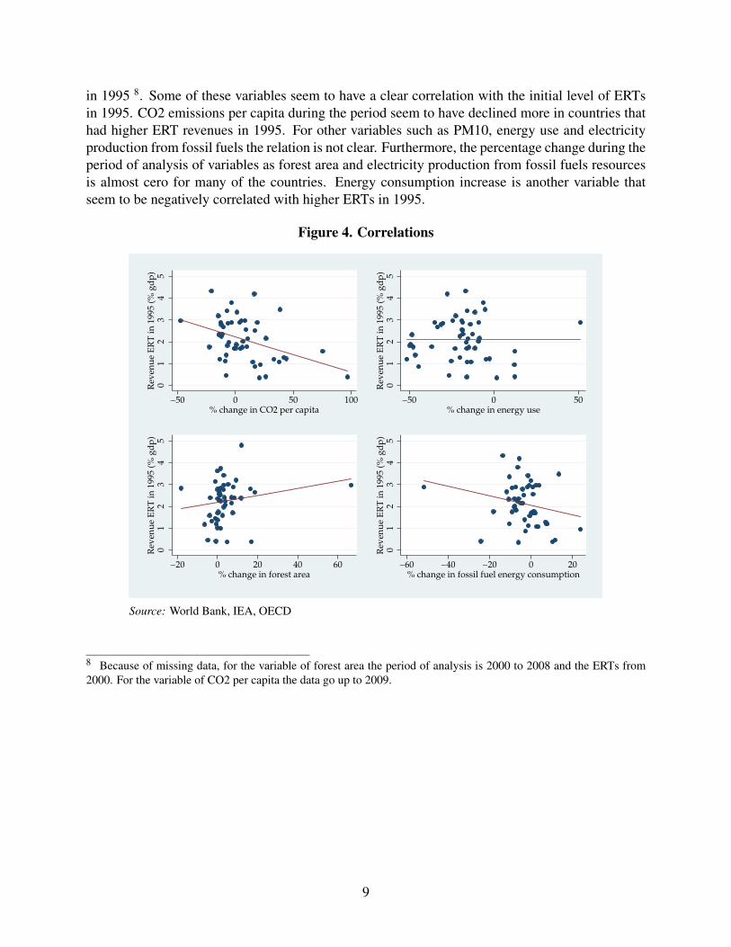
in 1995 8. Some of these variables seem to have a clear correlation with the initial level of ERTsin 1995. CO2 emissions per capita during the period seem to have declined more in countries thathad higher ERT revenues in 1995. For other variables such as PM10, energy use and electricityproduction from fossil fuels the relation is not clear. Furthermore, the percentage change during theperiod of analysis of variables as forest area and electricity production from fossil fuels resourcesis almost cero for many of the countries. Energy consumption increase is another variable thatseem to be negatively correlated with higher ERTs in 1995.

Figure 4. Correlations

01

23

45

Rev

enu

e E

RT

in

199

5 (%

gd

p)

−50 0 50 100% change in CO2 per capita

01

23

45

Rev

enu

e E

RT

in

199

5 (%

gd

p)

−50 0 50% change in energy use

01

23

45

Rev

enu

e E

RT

in

199

5 (%

gd

p)

−20 0 20 40 60% change in forest area

01

23

45

Rev

enu

e E

RT

in

199

5 (%

gd

p)

−60 −40 −20 0 20% change in fossil fuel energy consumption

Source: World Bank, IEA, OECD

8 Because of missing data, for the variable of forest area the period of analysis is 2000 to 2008 and the ERTs from2000. For the variable of CO2 per capita the data go up to 2009.

9

Figure 5. Correlations (cont)

01

23

4R

even

ue

ER

T i

n 1

995

(% g

dp

)

−60 −40 −20 0% change in PM10

01

23

4R

even

ue

ER

T i

n 1

995

(% g

dp

)

−200 0 200 400 600% change in electricity prod. from fossil fuels

01

23

4R

even

ue

ER

T i

n 1

995

(% g

dp

)

0 5000 10000 15000 20000 25000% change in electricity prod. from renewable sources

01

23

4R

even

ue

ER

T i

n 1

995

(% g

dp

)

0 50 100 150 200% change in electric power consumption

Source: World Bank, IEA, OECD

4.2 Other VariablesSeveral authors have analyzed different variables that may affect the change in pollution. The firstvariable that may impact the change in environmental variables is the level of GDP per capita inPPP constant prices. This variable measures the level of wealth and has been used in various em-pirical studies (Jobert et al. , 2002, Martin , 2008, e.g.,). Industrial intensity is also used as a proxyof the weight of polluting sectors in the economy. Economic growth, measured by GDP growth,has also been found to affect the level of pollution. As analyzed by Lin and Li (2011), the level ofurbanization (percentage of population in urban areas) will be used. Finally, to include a level ofenvironmental stringency, a dummy for countries with high regulatory stringency for the pollutantsfrom automobiles9.

5 Cross-Sectional Regressions5.1 MethodologyThe aim of the following empirical section is analyze the correlation of the change in differentenvironmental or energy variables with the initial level of ERT. The achievement in environmentalprotection coming from environmental policies is determined mainly by its effects on the devel-opment and spread of new technologies (Kneese and Schultze , 1975). In this way, it is necessary

9 The index was constructed by Perkins and Neumayer (2012) is used, and it is coded on a scale from 0 to 5. In thiscase it was transformed into a dummy for countries with regulation above 3.

10

to consider longer periods when looking for the effects of ERT. In particular, this first regressionconsiders a period of 15 years for most of the variables. Different models of regressions will beused to analyze these relationships. At first, the following model is estimated:

ln

(EV2010EV1995

)= α + βEV1995 + γERT1995 + δX + ε (1)

where EV is one of the nine environmental variables mentioned above. Therefore, nine regres-sions are estimated to determine the change during the period between 1995 and 2010 10. Theinitial level of the environmental variable will be included in the regressors; the reason will beexplained in further detail in the next section. The main variable of interest will be ERTs in theinitial year. Finally, X includes all the control variables. In this first part, only GDP per capita in1995, GDP growth, and the percentage of urban population will be used 11 and ε the error term.

5.2 ResultsTable 1 shows the nine estimations for each variable measuring environmental performance. Mostof the signs of the coefficients of the ERTs variable show that revenue from ERTs is correlatedwith better environmental performance. Higher levels of revenue from environmentally relatedtaxes are associated with a decrease in the level of CO2 emissions per capita, energy consumption,fossil fuel energy consumption, water pollutants and PM10. At the same time, greater revenuesfrom ERTs in the initial year are positively correlated with increase in forest area and electricityproduction from renewable sources. The coefficients of revenue from ERTs in 1995 are statisticallydifferent from zero when using the percentage change of CO2 emissions per capita and PM10 asdependent variables12.

10 Because of missing data, the period of analysis for the estimation using the variable of forest area is from 2000 to2010; when using water pollutants the period goes from 1995 to 2002; data on CO2 emissions per capita go from 1995to 2009.11 Robustness checks including as variables environmental stringency, environmental concern, energy use, industrialintensity and a dummy for Western European countries were also estimated.12 Regressions are robust when changing some of the controls.

11

Table 1. Regressions Using Percentage Change of the Variables

(1) (2) (3) (4) (5) (6) (7) (8) (9)VARIABLES CO2pc PM10 Water pol Energy Electricity F Fuel Fossil El Renew. El Forest

ERT95 -0.0730** -0.0414* -0.0462 -0.0194 0.0440 -0.0231 0.00710 13.88 0.000862(0.0334) (0.0235) (0.0523) (0.0261) (0.0702) (0.0196) (0.131) (13.18) (0.0122)

Dependent variable95 -0.0164 0.000709 -4.78e-09 -0.000299 4.88e-06 0.00144 -2.05e-05 -0.0283*** -0.00172(0.0102) (0.000515) (3.23e-08) (0.000617) (2.66e-05) (0.00174) (5.54e-05) (0.0103) (0.00108)

lnGDPpercap95 0.00730 0.0516 -0.0553 -0.0373 -0.387* -0.0326 -0.730* -10.03 0.0360(0.0957) (0.0481) (0.0868) (0.0444) (0.221) (0.0306) (0.412) (22.18) (0.0233)

GDP growth 0.0249 -0.191** -0.0301 -0.317** 0.369 -0.0783 0.0325 76.49* 0.110***(0.124) (0.0939) (0.131) (0.147) (0.252) (0.0601) (0.509) (41.03) (0.0379)

Urban population -0.105 -0.119 0.201 0.115 0.619 -0.0675 2.428 22.03 0.0401(0.355) (0.191) (0.309) (0.259) (0.560) (0.141) (1.878) (36.21) (0.127)

Constant 0.337 -0.631 0.498 0.327 3.434* 0.303 5.540* 50.69 -0.315(0.855) (0.489) (0.979) (0.390) (1.791) (0.367) (3.105) (192.0) (0.254)

Observations 50 49 40 50 50 50 49 49 50R-squared 0.255 0.207 0.070 0.311 0.266 0.149 0.204 0.189 0.164

Robust standard errors in parentheses*** p<0.01, ** p<0.05, * p<0.1

The coefficients suggest that revenue from ERTs is a good proxy of the level of taxes, dis-couraging the consumption of pollution inputs and reducing emissions of CO2 and PM10. Movinga country from the first to the fifth quintile of the distribution of revenues from ERTs in 1995 im-plies on average a decrease in the growth rate of CO2 emissions per capita and PM10 by 12.2% and6.9% points, respectively, over the 15-year sample period. With respect to the variables of energyand fossil fuel consumption, the lower growth rate is 3.2% points and 3.8% points, respectively.On the other hand, the results would imply an increase in the growth rate of forest area, electric-ity production from renewable sources, electricity power consumption, and electricity productionfrom fossil sources of 0.1, 23.3, 7.3 and 0.1 percentage points, respectively 13.

5.3 Disaggregation of ERTTaking into account the variety of taxes, Table 2 disaggregates revenue from ERTs into threemain taxes: energy taxes, transport taxes and pollution taxes. The information is available forthe period of analysis for only one set of countries, all European14. Energy taxes include taxeson energy products for transport purposes such as petrol, diesel, natural gas and others, and taxeson energy products for stationary purposes (coal, biofuels, heavy fuel oil, electricity consumptionand production, and district heat consumption and production, among others). Transport taxesinclude taxes on motor vehicles, road use, congestion taxes, flights, use of motor vehicles andother means of transport. Finally, pollution taxes include taxes for emissions in the air (NOx,SO2 contents, etc.), for ozone-depleting substances, for effluents to water, water pollution, waterpollution and noise. The other classification of taxes includes resource taxes, in particular taxes onwater abstraction, timber, fishing, extraction of raw materials and other resource extraction. Thisfinal classification was computed together with pollution taxes.

13 In A of the Appendix the same regression is estimated as in Table A.4 but using a Seemly Unrelated Regression(SUR) model. The reason for estimating a SUR is the possible existence of correlated errors across the equations andtherefore the efficiency of the estimator could be increased. The sample period for this regression is 1995 to 2008because of missing years in the variables for forest area and water pollutants.14 Data from Eurostat

12

The results using the change in CO2 emissions per capita are presented in Table 2. Thesame variable controls were included as in Table 1 but, given that this disaggregation of revenue isnot available for all countries, there are fewer observations than in the previous estimates. Higherrevenue from energy taxes is negatively correlated with the increase of CO2 emissions per capitaand significant, and the same occurs with revenues from pollution taxes. On the other hand, thecoefficient is positive for transport taxes, but the null hypothesis of being zero is not rejected.

Table 2. Regression with Disaggregated Taxes Using CO2 Emissions Per Capita as DependentVariable

(1) (2) (3) (4)VARIABLES

energy tax95 -0.0643* -0.0502(0.0357) (0.0456)

transport tax95 0.0477 0.0192(0.0403) (0.0434)

pollution tax95 -0.157 -0.202(0.108) (0.122)

Observations 28 28 25 25R-squared 0.449 0.456 0.429 0.466

Robust standard errors in parentheses*** p<0.01, ** p<0.05, * p<0.1

Including all Controls

6 GMM System Regressions6.1 MethodologyThe aim of this section is to estimate a dynamic panel model and to avoid inconsistent estima-tors once the lagged regressor is introduced. For this purpose Generalized Methods of Moments(GMM), proposed by Blundell and Bond (1998) and based on the Arellano-Bond method, areused. A two-step estimator is applied, using the level equation and the first difference regressionequation, where the first order difference variables and the lagged variables are employed as in-strument variables for the level and first difference equation, respectively 15. As explained above,the effects of environmental policy should be long term and it is therefore preferable to considerperiods longer than a year. For this panel, periods of two and four years will be used 16.

The following model will be estimated to capture the effect of the growth of each environ-mental or energy variable during the last two or four years:

15 The assumption of E(yi,s∆εi,t) = 0 and of E(∆yi,tεi,s) = 0 for s ≥ t − d are necessary, where d is the intervallagged periods used in the regression.16 Regressions for a three-period interval was also estimated and showed similar results.

13

ln

(EVtEVt−d

)= α− blnEVt−d + γERTt−d + ηlnGDPt−d + δXt + θt + εit where d = 2, 4 (2)

b = 1− e−β where β captures the speed of convergence. X represents the control variables includ-ing GDP growth during the last 2 or 4 years, industrial intensity, urban population and a dummy forhigh regulation in pollutants from automobiles as a proxy of environmental regulatory stringency.θ captures time fixed effects.

6.2 ResultsTables 3 and 4 show the GMM estimations using a period lag of two and four years17. Thep values from the AR test show that the second order residuals are not correlated and thereforethe estimators are consistent. Likewise, the p value from the Hansen test implies validity of theinstruments as the instruments appear to be exogenous for all regressions.

The main findings for the first table can be summarized as follows. The growth rates of CO2emissions per capita, energy consumption, fossil fuel consumption, PM10, electricity productionfrom fossil sources and water pollution are negatively correlated with the lagged level of revenuefrom ERT. On the other hand, the growth rates of electricity consumption and electricity productionfrom renewable sources are positively correlated. Coefficients are significant with a 95% level ofconfidence when using CO2 emissions per capita, PM10, electricity production from fossil sourcesand electricity production renewable sources as dependent variables 18. For an average country, anincrease of revenue from ERTs as percentage of GDP by 1% point implies a reduction in 5.4%points in the growth rate of CO2 emissions during the two next years.

In Table 4, the growth of CO2 emissions per capita, energy use and electricity productionfrom fossil sources continue to present negative correlation with the variable of ERT19. Contraryto previous estimations, the coefficient of the lagged revenue from ERTs and the growth rate offossil fuel consumption and PM10 are now positive. For the former, the coefficient is significantlydifferent from zero, but in the latter the coefficient is not statistically different from zero. Onaverage, an increase of one percentage point of revenue from ERTs as a percentage of GDP isassociated with an increase in electricity production from renewable sources in 33% points. Incontrast, the same increase implies a reduction in 16% and 14% points in the growth rate of CO2emissions per capita and energy consumption, respectively.

17 For the variable of forest area the GMM estimation was not made because there are only two or three observationsper country (for the years 2000, 2005 and 2010).18 Estimations are robust when modifying controls and excluding time fixed effects.19 Because of many missing years for the variable for water pollutant, the regression using an interval period of fouryears was not estimated.

14

Table 3. Panel GMM Estimation Using Interval Periods of Two Years

(1) (2) (3) (4) (5) (6) (7) (8)VARIABLES CO2pc PM10 Water pol Energy Electricity F Fuel Fossil El Renew. El

ERT−2 -0.0542** -0.0804*** -0.0614 -0.0206 0.00823 -0.00605 -0.214* 0.296**(0.0261) (0.0271) (0.0449) (0.0197) (0.0228) (0.00747) (0.125) (0.137)

Dependent variable−2 -0.289*** -0.0399 0.0159 -0.128** -0.183*** 0.0711 0.0610 -0.511***(0.104) (0.0679) (0.0312) (0.0480) (0.0483) (0.0578) (0.0461) (0.114)

lnGDPpercap−2 0.280*** 0.0480 0.0286 0.0121 0.200*** 0.00741 0.205 0.287(0.0976) (0.0438) (0.0485) (0.0182) (0.0687) (0.00734) (0.126) (0.419)

GDP growth 1.087*** 0.0975 0.543 -0.210 0.778*** 0.178*** 1.908* -4.159(0.186) (0.171) (0.371) (0.144) (0.117) (0.0474) (1.081) (2.486)

Observations -2.147*** -0.165 -0.359 0.519 -0.631** -0.379 -3.248* 6.586*(0.787) (0.606) (0.710) (0.358) (0.280) (0.263) (1.718) (3.571)

Observations 275 269 172 303 275 303 296 276Number of country id 48 47 37 48 48 48 48 47AR(2) 0.00124 0.00655 0.0373 0.000487 0.0374 0.00140 0.00358 0.0590AR(4) 0.341 0.670 0.329 0.816 0.486 0.190 0.0245 0.289Hansen Test 0.914 0.671 0.678 0.862 0.763 0.991 0.897 0.990

Robust standard errors in parentheses*** p<0.01, ** p<0.05, * p<0.1

Controls: Industrial intensity, urban population, high regulation dummy. Including constant and time fixed effects

Table 4. Panel GMM Estimation Using Interval Periods of Four Years

(1) (2) (3) (4) (5) (6) (7)VARIABLES CO2pc PM10 Energy Electricity F Fuel Fossil El Renew. El

ERT−4 -0.162*** 0.0114 -0.143** 0.0661 0.0314* -0.111 0.336(0.0587) (0.0231) (0.0538) (0.0572) (0.0174) (0.257) (0.307)

Dependent variable−4 -0.0921 0.215** -0.0326 -0.0770 0.417*** 0.224** -0.462**(0.138) (0.0808) (0.137) (0.198) (0.133) (0.104) (0.190)

lnGDPpercap−4 0.200 0.118** 0.109** 0.0127 -0.00836 0.0159 0.115(0.139) (0.0555) (0.0456) (0.256) (0.0278) (0.275) (0.516)

GDP growth 0.746** 0.237 -0.306 0.296 0.131 0.330 -2.449(0.310) (0.234) (0.269) (0.364) (0.130) (1.167) (2.749)

Observations 123 120 123 123 123 120 108Number of country id 48 47 48 48 48 47 46AR(4) 0.221 0.00372 0.102 0.185 0.00753 0.109 0.0760AR(8) 0.646 0.879 0.653 0.482 0.800 0.930 0.347Hansen Test 0.517 0.526 0.295 0.701 0.380 0.734 0.682

Robust standard errors in parentheses*** p<0.01, ** p<0.05, * p<0.1

Controls: Industrial intensity, urban population, high regulation dummy. Including constant and time fixed effects

7 ConclusionTable 5 summarizes all the previous estimations according to each environmental or energy vari-able and includes the coefficient signs of the estimators. The most notable result from all estima-tions is the effect of ERTs on the growth of CO2 emissions per capita: all estimations show a clearnegative relation between revenue from ERTs and the growth of this variable. As CO2 emissionsare driven by a variety of economic activities, it is therefore not surprising to find that this variable

15

is the one most affected by the level of total ERTs. It could be useful for future analysis to study theeffect of ERTs on each economic activity on the CO2 emissions generated by that specific activity.

The results from energy use as a dependent variable are also very robust and significantfor some estimations. PM10, with the exception of the last estimation, also shows also a negativeand significant correlation. Higher revenue from ERTs is also associated with lower electricityproduction from fossil sources but higher production from renewable sources. On the other hand,electricity consumption seems to have grown more in countries with higher revenues from ERT.

Table 5. Effects of ERTs Using Different Estimations

Dependent Variable(% change)

CrossSection

Regression

SURestimation

GMM 2lags

estimation

GMM 4lags

estimationCO2 emissions percapita

− ∗ ∗ −∗ − ∗ ∗ − ∗ ∗∗

Energy use − − − − ∗ ∗PM10 −∗ − − ∗ ∗∗ +Electricity productionfossil sources

+ − −∗ −

Water pollutant − −Fossil fuel energy con-sumption

− − − +∗

Electric power con-sumption

+ + + +

Electricity prod. fromrenewable sources

+ + + ∗ ∗ +

Forest area +*** p<0.01, ** p<0.05, * p<0.1

Countries with higher revenues from ERTs seem to perform better in the environmental do-main. This means lower emissions, including CO2 and PM10 levels, decreasing water pollutants,and reducing energy consumption and production, especially from fossil fuel sources. Revenuesfrom ERTs come mainly from fuel taxes, and most of these taxes were introduced to increase rev-enues rather than reduce fuel consumption or improve environmental quality. These results suggestthat, while fuel taxes may not be as effective or efficient as the literature had argued, they did havesome impact on environmental quality. For example, higher fuel taxes can lead to higher fuel effi-ciency, and it seems to do so when long-run impacts are analyzed, as this study does. Additionally,the effects on pollution can be at a local level, as shown with PM10, or at a more national levelas occurs with CO2 emissions. Although previous studies have questioned the effectiveness ofERTs and highlighted their inefficiencies, the results from this work show that, despite all, ERTsare effective. Therefore, this market-based instrument has considerable potential for dealing withenvironmental problems.

16

ReferencesAlbrecht, J. 2006. “ The Use of Consumption Taxes to Re-Launch Green Tax Reforms.” Interna-

tional Review of Law and Economics 87(1): 115-143.

Baumol, W.J., and W.E. Oates. 1988. The Theory of Environmental Policy. Cambridge, UnitedKingdom: Cambridge University Press.

Blundell, R., and S. Bond. 1998. “Initial Conditions and Moment Restrictions in Dynamic PanelData Models.” Journal of Econometrics 87(1): 115-143.

Brannlund, R., and J. Nordstrom. 2004. “Carbon Tax Simulations Using a Household DemandModel.” European Economic Review 48(1): 311-333.

Brannlund, R., and T. Lundgren. 2010. “Environmental Policy and Profitability: Evidence fromSwedish Industry.” Environmental Economics and Policy Studies 12: 59-78.

Brons, M. et al. 2008. “A Meta-Analysis of the Price Elasticity of Gasoline Demand: A SURApproach.” Energy Economics 30(5): 2105-2122.

Bruvoll, A., and B.M. Larsen. 2004. “Greenhouse Gas Emissions in Norway: Do Carbon TaxesWork?” Energy Policy 32(4): 493-505.

Convery, F., S. McDonnell and S. Ferreira. 2007. “The Most Popular Tax in Europe? Lessonsfrom the Irish Plastic Bags Levy.” European Association of Environmental and ResourceEconomists 38(1): 1-11.

Deyle, R.E., and S.I. Bretschneider. 1995. “Spillovers of State Policy Innovations: New York′sHazardous Waste Regulatory Initiatives.” Policy Analysis and Management 14(1): 79-106.

Di Cosmo, V., and M. Hyland. 2011. “Carbon Tax Scenarios and their Effects on the Irish EnergySector.” Working Paper 407. Dublin, Ireland: Economic and Social Research Institute.

Gerlagh, R., and B. van der Zwaan. 2006. “Options and Instruments for a Deep Cut in CO2 Emis-sions: Carbon Dioxide Capture or Renewables, Taxes or Subsidies?” Energy Journal 27(3): 25-48.

Goulder, L. H. 1995. “Environmental Taxation and the Double Dividend: A Reader′s Guide.”International Tax and Public Finance 2: 157-184.

Jaffe A. B., Newell, R. G., and R.N. Stavins. 2002. “Environmental Policy and TechnologicalChange.” Environmental and Resource Economics 22(2): 41-69.

Jobert, T., F. Karanfil and A. Tykhonenko. 2010. “Convergence of Per Capita Carbon Dioxide inthe EU: Legend or Reality?.” Energy Economics 32(6): 1364-1373.

Kneese, A., and C. Schultze. 1975. “Pollution, Prices, and Public Policy.” Washington, DC, UnitedStates: Brookings Insititution.

Levinson, A. 2003. “Environmental Regulatory Competition: A Status Report and Some NewEvidence.” National Tax Journal 56(1): 91-106.

17

Liang, Q.M., Y. Fan and Y.M. Wei. 2007. “Carbon Taxation Policy in China: How to ProtectEnergy-and Trade-Intensive Sectors?” Journal of Policy Modeling 29(2): 311-333.

Lin, B., and X. Li. 2011. “The Effect of Carbon Tax on Per Capita CO2 Emissions.” Energy Policy39 (9): 5137-5146.

Martin, W. 2008. “The Carbon Kuznets Curve: A Cloudy Picture Emitted by Bad Econometrics?”Resource and Energy Economics 30(3): 388-408.

Nakata, T., and A. Lamont. 2001. “Analysis of the Impacts of Carbon Taxes on Energy Systems inJapan.” Energy Policy 29(2): 159-166.

Newberry, D.M. 2004. “Road User and Congestion Charges.” In: S. Cnossen, (ed.), Theory andPractice of Excise Taxation. Oxford, United Kingdom: Oxford University Press.

O′Brien, P., and A. Vourc’h. 2002. “Encouraging Environmentally Sustainable Growth: Experi-ence in OECD Countries.” Empirica 29(2):93-111.

O′Ryan, R., S. Miller and C. de Miguel. 2003. “A CGE Framework to Evaluate Policy Optionsfor Reducing Air Pollution Emissions in Chile.” Environment and Development Economics8(2):285-309.

OECD. 2001.Environmentally Related Taxes in the OECD Countries: Issues and Strategies. Paris,France: Organisation for Economic Co-operation and Development.

OECD. 2006. The Political Economy of Environmentally Related Taxes. Paris, France: Organisa-tion for Economic Co-operation and Development.

Parry, I., and K. Small. 2004. “Does Britain or the United States Have the Right Gasoline Tax?”Discussion Paper 0212 rev. Washington, DC, United States: Resources for the Future.

Perkins, R., and E. Neumayer. 2012. “Does the California Effect Operate across Borders? Trading-and Investing-up in Automobile Emission Standards.” Journal of European Public Policy19 (2): 1350-1763.

Pigou, A. 1920. The Economics of Welfare. London, United Kingdom: Macmillan.

Porter, M.E. 1991. “America’s Green Strategy.” Scientic American 268(4):168.

Sigman, H. 2003. “Taxing Hazardous Waste: The U.S. Experience.” Public Finance Management3(1): 12-33.

Sumner, J., L. Bird and H. Smith. 2009. “Carbon Taxes: A Review of Experience and PolicyDesign Considerations.” Technical Report NREL/TP-6A2-47312. Golden, United States:National Renewable Energy Laboratory.

Sterner, T. 2007. “Fuel Taxes: An Important Instrument for Climate Policy.” Energy Policy 35(6):3194-3202

18

Vehmas, J. 2005. “Energy Related Taxation as an Environmental Policy Tool: The Finnish Experi-ence 1990-2003.” Energy Policy 33(17): 2175-2182.

West, S.E., and R.C. Williams III. 2004. “Estimates from a Consumer Demand System: Implica-tions for the Incidence of Environmental Taxes.” Journal of Environmental Economics andManagement 47(3): 535-558.

Wier, M. et al. 2005. “Are CO2 Taxes Regressive? Evidence from the Danish Experience.” Eco-logical Economics 52(2): 239-251.

Wissema, W., and R. Dellink. 2007. “AGE Analysis of the Impact of a Carbon Energy Tax on theIrish Economy.” Ecological Economics 61(4): 671-683.

Yan, X.Y., and R.J. Crookes. 2009. “Reduction Potentials of Energy Demand and GHG Emissionsin Chinas Road Transport Sector.” Energy Policy 37(2): 658-668.

A Appendix Tables

Appendix Table A.1. List of variables

Variable Meaning Mean SD Sourceert pgdp Revenues from ERT’s as perc.

of GDP2.4 0.8 OECD, Eurostat

CO2 pc CO2 emissions (metric tonsper capita)

7.6 4.4 World Bank

Forest Forest area (perc. of landarea)

32.6 18.2 World Bank

Energy Energy use (kg of oil eq.) per1000 GDP (const. 2005 PPP)

170 73.8 IEA

combustible renewable Combustible renewables andwaste (perc. of total energy)

8.6 9.6 IEA

F Fuel Fossil fuel energy consump-tion (perc. of total)

76.4 16.8 IEA

Electricity Electric power consumption(kWh per capita)

6,387.2 5,764.6 IEA

Water pol Organic water pollutant(BOD) emissions (kg perday)

334,294.8 942,027.2 World Bank

PM10 PM10, country level (micro-grams per cubic meter)

34.6 25.6 IEA

Fossil El Electricity production fromoil and coal sources (kWh percapita)

2179.9 2159.8 IEA

Renew. El Electricity prod. from renew-able sources(kWh per capita)

364.2 1171.4 IEA

gdp growth GDP growth (annual perc.) 3.8 3 World Bankln gdp per cap ln GDP per capita, PPP (const

2005 int.)9.77 0.66 World Bank

Urban population Percentage of urban popula-tion

0.71 0.15 World Bank

industrial intensity Industrial value / gdp 2.7% 6.3% World BankRD Research and development

expenditure (per. of gdp)1.4 1 World Bank

environmenta concern Per. of population thatstrongly agree to give parttheir income and accept an in-crease in taxes for the envi-ronment

9.5% 5.2% World Value Survey

ESI2002 Environmental sustainabilityindex in 2002

62.4 15.2 World Economic Fo-rum, Yale Center forEnvironmental Lawand Policy, and CIESIN

High regulation Dummy for countries about 3in the scale from 0 to 5 ofregulation stringency for au-tomobile pollutants

0.49 0.50 Perkins and Neumayer(2012)

Source: OECD, Eurostat, World Bank, IEA

20

Appendix Table A.2. Environmental Variables: Percentage Change between 1995 and 2010

Variable Mean SD Min MaxGrowth of CO2 emis-sions per capita

7.1 24.7 -47.3 96.8

Growth of energy use -19.3 15.5 -57.7 32.5Growth of fossil fuelconsumption

-2.2 9.4 -44.1 17.6

Growth of PM10 -31.2 12.3 -56.3 -9.1Growth of electricityproduction from fossilsources

30.5 71.9 -98.9 120.6

Growth of electricityproduction from renew-able sources

919.6 154.3 -42.1 6530.1

Growth of electricityconsumption

41.6 45.0 -3.9 187.8

Source: World Bank, IEA

Appendix Table A.3. Regressions Using Revenue from ERTs (as percentage of GDP) againstEnergy Taxes (constant US dollars, using PPP, per unit)

Revenue from ERTsERT varible Coefficient Std. ErrorLight Fuel Oil 0.0015 0.0001***Diesel 1.83 0.114***Premium Leaded 2.07 0.151***Unleaded Gasoline 1.83 0.098***High Sulfur Oil 0.01 0.001***Natural Gas 0.19 0.018***Steam Coal 0.003 0.003Coking Coal 0.03 0.006***Electricity 0.01 0.004***

Robust standard errors in parentheses*** p<0.01, ** p<0.05, * p<0.1

Note: All estimations include time and country fixed ef-fects. Units: sulfur fuel oil, steam coal and coking coalin tons; light fuel oil in thousand liters; diesel, unleadedand leaded gasoline in liters; natural gas and electricity inMWh.

21

Appendix Table A.4. SUR using percentage change of the variables

(1) (2) (3) (4) (5) (6) (7)VARIABLES CO2pc PM10 Energy Electricity F Fuel Fossil El Renew. El

ERT95 -0.0673* -0.0363 -0.0169 0.0492 -0.0145 -0.0132 9.685(0.0400) (0.0247) (0.0271) (0.0756) (0.0186) (0.199) (6.166)

Dependent variable95 -0.0106 0.000281 -0.000201 -5.51e-06 .000425 -2.38e-05 -0.0131(0.00863) (0.00102) (0.000380) (2.32e-05) (0.000981) (8.36e-05) (0.0180)

lnGDPpercap95 -0.0490 0.0395 -0.0348 -0.324 -0.0471** -0.940* -5.181(0.101) (0.0480) (0.0421) (0.200) (0.0233) (0.537) (10.54)

GDP growth 0.0292 -0.157** -0.301*** 0.266 -0.0727 -0.619 52.40***(0.140) (0.0707) (0.0753) (0.231) (0.0455) (0.500) (18.06)

Urban population -0.0430 -0.0583 0.174 0.644 -0.0468 3.515 15.28(0.364) (0.167) (0.226) (0.565) (0.126) (2.420) (23.81)

Constant 0.781 -0.516 0.237 2.920* 0.499** 7.294* 13.57(0.877) (0.471) (0.373) (1.721) (0.233) (3.987) (93.91)

Observations 48 48 48 48 48 48 48R-squared 0.260 0.227 0.423 0.215 0.197 0.220 0.288

Standard errors in parentheses*** p<0.01, ** p<0.05, * p<0.1

Robust Standard errors

22

Appendix Table A.5. Countries

country MeanERTs % Revenue ERTs % GDP CO2 emissions (metric tons per cap) GDP per capita

Argentina 5.2% 1.3% 4.0 10564Australia 8.0% 2.3% 17.7 30201Austria 5.9% 2.5% 8.2 31890Belgium 5.1% 2.3% 10.8 30448Brazil 5.7% 1.9% 1.9 8218Bulgaria 2.5% 6.2 8322Canada 4.0% 1.4% 16.6 32474Chile 7.0% 1.4% 3.8 11684China 4.5% 0.7% 3.5 3306Colombia 2.2% 0.3% 1.5 7070Costa Rica 7.8% 1.6% 1.5 8460Cyprus 3.1% 7.3 23041Czech Republic 7.6% 2.7% 12.0 19027Denmark 9.6% 4.7% 9.9 31613Dominican Republic 15.0% 2.1% 2.2 5937Estonia 5.7% 1.7% 12.6 13333Finland 6.9% 3.1% 11.4 27964France 4.9% 2.1% 6.2 28123Germany 6.6% 2.4% 10.3 30444Greece 7.0% 2.3% 8.4 21768Guatemala 6.9% 0.9% 0.9 3983Hungary 7.7% 3.0% 5.7 14722Iceland 7.6% 2.8% 7.5 30970Ireland 8.6% 2.6% 10.3 37514Israel 8.2% 3.0% 9.1 22655Italy 7.5% 3.1% 7.8 27489Japan 6.4% 1.7% 9.6 29502Korea, Rep. 11.8% 2.7% 9.3 20130Latvia 2.3% 3.2 10364Lithuania 2.3% 4.1 11581Luxembourg 7.5% 2.8% 20.9 61486Malta 3.5% 6.6 20230Mexico 5.6% 0.9% 3.9 11601Netherlands 9.4% 3.7% 10.8 33515New Zealand 4.6% 1.6% 8.1 23169Norway 7.2% 3.0% 8.8 44526Peru 5.9% 0.9% 1.2 6025Poland 5.6% 1.9% 8.3 12358Portugal 9.8% 3.0% 5.8 20586Romania 2.4% 4.6 8320Slovak Republic 6.5% 2.2% 7.4 14447Slovenia 7.2% 3.2% 7.8 21019South Africa 10.1% 2.7% 8.6 8132Spain 6.0% 2.1% 7.3 25338Sweden 5.8% 2.8% 5.9 29772Switzerland 7.1% 2.0% 5.6 34747Turkey 12.2% 2.9% 3.4 10318United Kingdom 7.8% 2.7% 9.2 29790United States 3.5% 1.0% 19.2 39547Uruguay 6.4% 1.4% 1.7 9564Total 7.1% 2.4% 7.6 21028

Source: OECD, Eurostat, World Bank, IEA

23