Embed Size (px)
Citation preview
Are Consumers Affected by Durable Goods Makers’ Financial Distress?
The Case of Auto Manufacturers+∗
Ali Hortaçsu Department of Economics, University of
Chicago and NBER [email protected]
Gregor Matvos University of Chicago Booth School of
Business [email protected]
Chad Syverson University of Chicago Booth School of
Business and NBER [email protected]
Sriram Venkataraman Goizueta Business School, Emory
University [email protected]
Abstract Theory suggests the financial decisions of durable goods makers can impose spillovers on their consumers. Namely, the consumption stream that durable goods provide frequently depends on services provided by the manufacturer itself (e.g., warranties, spare parts availability, maintenance and upgrades). Manufacturer bankruptcy, or even the possibility thereof, threatens this service provision and as a result can substantially reduce the value of its products to their current owners. We test whether this hypothesis holds in one of the largest durable goods markets, automobiles. We use data on prices of millions of used cars sold at wholesale auctions around the U.S. during 2006-8. We find that an increase in an auto manufacturer’s financial distress (as measured by an increase in its CDS spread) does result in a contemporaneous drop in the prices of its cars at auction, controlling for a host of other influences on price. The estimated effects are statistically and economically significant. Furthermore, cars with longer expected service lives (those within manufacturer warranty, having lower mileage, or in better condition) see larger price declines than those with shorter remaining lives. These patterns do not seem to be driven solely by reduced demand from auto dealers affiliated with the troubled manufacturers or by contemporaneous or future declines in new car prices or high frequency demand shocks. Our estimates also imply a potentially large indirect cost of financial distress on car manufacturers. + We thank Jonathan Berk, Judith Chevalier, Alessandro Gavazza, Antoinette Schoar and the participants of the Chicago Booth finance seminar, the NBER Industrial Organization and Corporate Finance meetings and the WFA meetings for comments and feedback. ∗ Contact information: Hortaçsu: Department of Economics, University of Chicago, 1126 E. 59th St., Chicago, IL 60637.; Matvos and Syverson: University of Chicago Booth School of Business, 5807 S. Woodlawn Ave., Chicago, IL 60637; Venkataraman: Goizueta Business School, Emory University, 1300 Clifton Road NE, Atlanta, Georgia 30322.

1
1. Introduction
Firms’ financial decisions have potential spillovers on consumers of durable goods. The
consumption stream that durable goods provide frequently depends on product warranties, the
availability of spare parts, maintenance, and upgrades. For example, a car owner relies on
warranties to cover malfunctions early in the car’s life, on car parts to be available when the car
breaks down, and on the presence of a dealer who can service the car.
As is the case in the car industry, the provision of these and similar services is frequently
vertically integrated into the manufacturer.1 If a car manufacturer were to go bankrupt, it may not
honor the warranties or provide parts and services in the future, reducing the consumption of the
durable goods owner.2
Even though these spillovers are potentially important and large, we have little empirical
evidence on the relationship between firms’ financial distress and the value of durable goods. It
is important to understand this relationship because durable goods represent a significant fraction
of household wealth. Automobiles, the subject of our study, account for about 5 percent of
consumption in the U.S. and are the nonfinancial asset most commonly held by households.
They represented roughly 3 percent of U.S. household wealth in 2007 (Bucks et al. (2009)). Any
variation in the value of these assets can expose households to wealth and consumption shocks.
In fact, the mere expectation of probable bankruptcy may reduce the
expected value of durable goods to a forward-looking consumer. Therefore, as firms experience
financial distress, they impose potentially large spillovers on those who own their goods.
Knowing how firms’ financial distress affects owners of durable goods is also critical to
understanding firms’ financial decisions. Forward-looking consumers understand that financial
distress decreases the probability that future warranties will be honored and parts and services for
their car will be available. This reduces demand for the cars of troubled manufacturers. In a 2006
survey, 23 percent of consumers who avoided the “Big 3” (more recently referred to as the 1 Provision of car warranties is generally vertically integrated into the manufacturer, who bundles the warranty with the car. Vertical integration may be natural in this case; it solves the asymmetric information problem present because car manufacturers are best informed about likely future claims on the cars they make. Furthermore, it effectively makes manufacturers the residual claimants on the effort expended toward increasing car durability. 2 In bankruptcy, warranties are general unsecured claims, in priority after secured claims and other priority claims. An example of this was seen in the marine engine industry with the Chapter 11 bankruptcy of former industry stalwart Outboard Marine Corp. in 2000. According to an article on the case (http://my.boatus.com/consumer/OMCBankruptcy.asp), the federal trustee assigned to the case said she had “never seen funds set aside in other bankruptcy cases for possible warranty claims in the future” and that while consumers with currently outstanding warranty claims would be able to file proof of claim forms with the court, even they would probably not be paid in full. Further, the article notes that companies that buy assets sold in bankruptcy auctions are not legally obligated to assume warranty liability for products made by the predecessor company.

2
“Detroit 3”) brands listed those companies’ financial conditions as a reason for avoidance (J.D.
Power (2006)). Because of these indirect costs of financial distress, firms may curb the amount
of debt used in financing despite the large tax advantages of debt financing.3
While the literature since Titman (1984) frequently appeals to indirect costs of financial
distress to explain why firms use little debt, there is little direct evidence of such indirect costs in
general or in durable goods demand in particular (Hotchkiss et al. (2008)). Measuring the effects
of financial distress on the demand for goods is empirically challenging because causality can
also operate in the opposite direction: negative demand shocks affect firms’ cash flows and
therefore can induce financial distress. This generic problem has plagued the literature on the
effects of financial distress and indirect costs of bankruptcy, whether these indirect cost are from
the consumer, supplier, or employee side.
4
Our study, besides focusing on an inherently interesting set of products and firms, can avoid
many of these identification issues. We study the impact of financial distress on the prices of
used cars in car auctions conducted by a major car auction house in the United States from
January 1, 2006 to November 14, 2008. We compare shifts in the prices of a manufacturer’s cars
to a measure of that manufacturer’s likelihood of bankruptcy. As we discuss below, we believe
our data is rich enough to provide sources of identification of the links between cars’ values and
their manufacturer’s financial distress that are unlikely to be driven by reverse causation, where
price drops lead to distress rather than vice versa.
Looking for such effects in used car auctions holds several advantages over new car markets.
Wholesale car markets are very liquid; prices can rapidly adjust to changes in the economic
environment. Their participants are knowledgeable about the product and the final demand
environment. Their decentralized nature makes them less exposed to strategic pricing.
To measure firms’ financial distress levels, we use credit default swaps (CDS) spreads. These
are securities whose payoffs are conditional on the firm defaulting on its debt, so their price
3 See Titman (1984) for an early discussion of indirect cost of financial distress. Graham (2000) explores the size of debt’s tax benefits. 4 Despite the lack of evidence, the U.S. Treasury Department certainly believed such indirect cost of financial distress have a large impact on car manufacturers, and through warranties in particular. On March 30, 2009, they announced the Warranty Commitment Program, which guaranteed warranties of new General Motors and Chrysler cars were the manufacturers to go bankrupt. They started the program to “help provide much needed certainty to consumers, and a boost to the auto industry, during the restructuring period.” We evaluate this assertion in this paper.
3
reflects the expected probability that a firm enters bankruptcy. Because they are much more
liquid than the bonds of the respective companies, they provide the most current measure of
companies’ financial distress.
We use several sources of variation to address the identification issues plaguing efforts to
measure the effect of financial distress on product demand. Our core specification estimates the
car price-CDS spread relationship using variation within detailed model-by-region-by-week
categories. For instance, we compare the price difference between a 2005 Ford Focus ST sold at
an Atlanta auction on Monday and a 2005 Ford Focus ST sold in Ft. Lauderdale later that same
week to the change in Ford’s CDS spread during the intervening days. Using high-frequency
variation makes it less likely that shifts in consumers’ views of a particular manufacturer, which
presumably operate at a lower frequency, create simultaneous price shifts and financial distress.
That said, we observe the negative correlation between a manufacturer’s CDS spread and its
used car prices at lower frequencies as well. Our basic specification indicates that a 1000-point
increase in a manufacturer’s CDS spread (a large change, but some firms experience even larger
ones in the data) drops the average price of its used cars by $68, or about 0.5 percent.
A further testable prediction of our setting is that financial distress should not affect all cars
to the same degree. Cars with longer expected remaining service lives should expectedly see a
greater price drop when a manufacturer risks bankruptcy, as their flow of lost services would be
greater. Further, if car owners worry that their warranties will not be honored upon bankruptcy,
then the value of these warranties (capitalized into the price of the car) will fluctuate with
manufacturers’ financial distress. These effects will imply that value of cars that are still covered
under manufacturer warranty or cars with lower mileage should be more affected by financial
distress. We find these patterns in the data. The interaction between a car’s mileage and its
manufacturer’s CDS spread is broadly negative, measured in several ways. We directly test for
warranty effects and find the CDS effect is significantly larger for cars in warranty.
It is, of course, possible that changes in manufacturer CDS spreads could affect the supply of
used cars. In their analysis of a similar used car auction data set to identify how fluctuations in
gasoline prices are reflected in the prices and market shares of cars, Busse, Knittel, and
Zettelmeyer (2010) point out that both the demand and supply of used cars with different fuel
efficiencies may respond differentially to such shocks. Our specifications therefore include
controls for supply-side movements. In particular, we show that the effect is not driven by

4
manufacturers’ fire sales of new cars, by the expectation of fire sales of new cars, or by the
financial distress of the dealers. We also explicitly incorporate proxies for high-frequency
demand shocks, and find our results to be robust.
We use our estimates to approximate the effect that financial distress has on manufacturers
through a decrease in demand for new cars. Using GM as a example, we find the potential size of
the effect substantial: even the most conservative estimates yield an 6 percent in GM car
margins, or alternatively, a 10 percent drop in value of the General Motors North America
vehicles division for a 3000 CDS point increase relative to Ford, which is what we observe in the
data.
1.1 Related Literature
Our paper touches on the previous literature in two distinct ways. First, it directly contributes
to the literature on firm capital structure and the indirect cost of financial distress. Since Titman
(1984), indirect costs have been used to rationalize the reluctance of firms to use debt financing
despite large tax benefits of debt. While we do not provide direct evidence that firms take
indirect costs of financial distress into account when choosing capital structure, our study
provides evidence regarding the existence and magnitude of indirect costs of financial distress. In
their classic paper, Andrade and Kaplan (1998) study thirty one leverage transactions to try to
identify the impact of financial distress on firm value. They estimate financial distress cost to be
from 10 to 20 percent of firm value. Our paper is closest to Chevalier (1995a, 1995b) and
Chevalier and Scharfstein (1996). They also use transaction-level data to study the interaction
between financial distress and market outcomes. Their focus is the relationship between
supermarkets’ financial structures and the pricing decisions in the industry, and in particular the
strategic effects of financial distress on entry and markups.
Second, the paper delves into the nature of durable goods markets. Most of the literature on
these markets has focused on the interaction between the market for new and used goods, trying
to understand the competition a monopolist faces from used goods she sold in the past.5
5 See Coase (1972), Bulow (1982), and Stokey (1981) for early work on the Coase conjecture.
Our
paper instead highlights the fact that much of the consumption stream from durable goods
depends on future commitments from the manufacturer and other providers of complementary
5
services. To understand the behavior of durable goods suppliers and consumers, we have to
understand the complex structure of services that accompany the consumption of durable goods.
The paper is structured as follows. In Section 2, we describe the market for used cars and
how it is organized though wholesale auctions. We then describe the data we are using and
provide descriptive statistics. In Section 3, we discuss our empirical specification. Section 4
presents and discusses our estimates. In Section 5, we discuss the implications of our estimates
for the indirect cost of financial distress on the case of GM. Section 6 concludes.
2. Institutional Background and Data
Each year, consumers in the United States buy close to 40 million used vehicles, three times
the number of new cars sold. In 2008, for example, there were 36.5 million used vehicle sales
(~$292 billion in revenues) and 13.2 million new vehicle sales (~$351 billion in revenues).
While a small fraction of the used vehicles are traded via private party transactions, the lion’s
share of the used car sales is transacted via the dealer networks. Of the 80,000 auto dealerships in
the U.S., nearly 60,000 sell only used cars, while the remaining dealers trade both new and old
cars.
These dealers acquire the bulk of their used car inventory via weekly used car auctions
conducted at various locations. The auctions are typically wholesale buyers only—they exclude
the end consumer.6
The top five auctioneers cumulatively command approximately an 80 percent market share in
the U.S. While each auctioneer varies in terms of regional distribution and size of operations at
each location, physical auction sites managed by major auctioneers are quite large. Each can
have between 10 and 100 lanes where automobiles are wheeled through as auctions take place.
In general, these transactions occur between purchasing dealers and other
firms that are car suppliers. Sellers include other dealers, auto manufacturers, rental car agencies,
and corporate fleet resellers. Dealers often rely on such auctions to adjust their used car
portfolios to changing local market conditions. Manufacturers use these auctions sell fleet and
program cars. Car rental agencies use these auctions to trade-in their used cars before they get
out of factory warranty. Sellers may also be financial institutions who use the wholesale auction
to reduce their inventory of program and repossessed cars.
6 Only licensed buyers and sellers who register with the auctioneer can participate in the auction.

6
Our wholesale auction data comes from a large multinational auctioneer. The firm is the
world’s largest provider of vehicle remarketing services and is one of the largest wholesale
automobile auctioneers in the U.S., operating eighty-three geographically dispersed auction sites.
We use data on over 6 million successfully completed transactions from January 1, 2006 through
November 14, 2008. The total value of these sales was about $89 billion, with an average
transaction price of $13,000 per car. The auctioneer runs one or two auction sessions per week at
each site, each lasting approximately five hours. Our auctioneer’s sites are quite large (see Figure
2a). Table 3 lists select sites and their respective traded volumes. They vary in size from one
dozen to several dozen lanes and in their volume of successful transactions.
On average, about 3000 cars sell at each auction location in a given day. Buyers can inspect
the car the parking lot prior to the auction session. Each car is provided with a car condition
report issued by the auctioneer. This and other vehicle details are prominently displayed in the
windshield of each vehicle. Professional auctioneers lead the bidding process, often in the
presence of the seller representative (see Figure 2b). When bidding ends, the auctioneer consults
the seller’s representative or some previously communicated reservation price to determine
whether the winning bid is accepted or rejected. Sold or not, the car is then wheeled out and a
new vehicle is wheeled in. The entire process takes about thirty seconds per car. Sometimes cars
that aren’t sold are wheeled back in later in the day. Others are re-auctioned on a future date or
even transferred to another site. We observe in the data how many times a car was wheeled in at
any auction location before it is sold, as well as sequence in which it was wheeled in (i.e., its run
number).
For buyers and sellers who cannot travel to the physical auction site, the firm also uses a
proprietary web-based technology that enables both sides of the market to participate in the live
physical auctions via real-time audio and video (Figure 2c). Physical auction lanes are equipped
with video cameras that allow online users to view the vehicle as it gets wheeled in, observe the
physical bidding activity and place their bids via the web. Online users’ bids are displayed on the
screen located in the physical lane. Large seller consignors like manufacturers and financial
institutions can also chose to sell their vehicles via an “upstream” channel that is operated and
managed by our market maker. This service gives sellers the ability to remarket their inventory
earlier in the remarketing cycle than physical auction lanes. Buyers save on time and travel
expenses with desktop access to “Bid or Buy Now” from the largest nationwide selection of

7
wholesale inventory available. Any unsold cars are moved to the physical auction site and sold
through the original process.
In our data, we know whether the winning bid was placed by an online bidder or in-lane
bidder or if the car was purchased in the upstream channel. As can be seen in Table 3,
approximately 82 percent of the transacted cars were sold to in-lane bidders, 15 percent via the
upstream channel, and the remaining to online bidders. Sometimes consignors restrict their sales
to select buyers only, referred to as “closed” sales. Closed marketplaces often serve to benefit a
manufacturer’s franchise dealer network. Unrestricted or open auctions attempt to allow for
maximum buyer participation. 76 percent of the transacted cars in our data were sold in
unrestricted auctions (Table 3).
67 percent of the completed transactions are fleet/lease sales, 28 percent factory owned sales,
and 5 percent are dealer-to-dealer sales (Table 3). Each automobile is identified by a
manufacturer issued unique vehicle information number (VIN). For each VIN we collected
information on a large set of vehicle characteristics including car make (Ford, Toyota, Honda,
etc.), model (Taurus, Explorer, Altima, etc.), body style (SUV V6, Midsize 4dr V6, 1500 Pickup
V12, etc.), and model year. Our data also include the odometer mileage reading and quality
condition of each vehicle as certified by the market maker. See Table 2 for details on the quality
rating scale.
We obtain the daily time-series of credit default swap spreads with five year maturity (CDS)
from Thompson Financial DataStream for all publicly traded automobile manufacturers during
the corresponding time period as our auctions data. Figure 3 plots the CDS time series for four
manufacturers: General Motors, Ford, Honda, and Toyota. The prices are in basis points, which
can be interpreted under risk neutrality as default probability. For example, a CDS of 1000 basis
points corresponds to 10 percent default probability.
We then match the appropriate CDS series to the auction transaction data using the
manufacturer identities in the auction database.7
7 This yields CDS series for the vast majority of brands in our data, including Acura, Audi, BMW, Buick, Cadillac, Chevrolet, Chrysler, Daewoo, Dodge, Ford, Geo, GMC, Honda, Hummer, Hyundai, Infiniti, Isuzu, Jaguar, Jeep, Land Rover, Lexus, Lincoln, Mazda, Mercedes Benz, Mercury, Mini, Mitsubishi, Nissan, Oldsmobile, Plymouth, Pontiac, Porsche, Saab, Saturn, Scion, Suzuki, Toyota and Volkswagen.
The matching of CDS data and transactions
yields a matched database containing 6,188,759 auto sales. Table 4 contains the descriptive
statistics of select variables for our final matched data. The data reflect significant variation in

8
price (mean = $13,062, median = $12,300, and s.d. = $7560) and CDS (mean = 643.1 and s.d. =
856.1). The cars vary by mileage, age, and quality condition—from relatively pristine to useful
only for salvage. Table 5 describes the price and CDS variation by quality condition (with 0
being salvage ready and 5 being very good), while Table 6 contains descriptive statistics by
mileage tiers.8
As expected, transacted prices fall with quality and age. Note, however, that
significant variation exists in the cross-conditions of these two variables; there is significant
mileage variation within quality tiers and quality variation within mileage tiers.
3. Empirical Specification
Our core specification to measure the effect of financial distress on used cars’ values is the
following:
𝑝𝑖𝑗𝑘𝑙𝑡 = 𝛽𝐶𝐷𝑆𝑖𝑡 + 𝑋𝑖𝑗𝑘𝑙𝑡𝛤 + 𝑎𝑖𝑗𝑘𝑇 + 𝜀𝑖𝑗𝑘𝑙𝑡,
where i indexes manufacturer; j indexes car model, trim, and model year (we will refer to any
unique combination of i and j as a “car type”); k indexes auction location (which in most
specifications will be one of eight regions in the U.S.), l indexes the specific auction at which the
car is sold, t indexes day, and T indexes week. Our dependent variable is the transaction price of
the car at auction pijklt, though we will also estimate specifications below that use a normalized
price that divides the transaction price by the average sales price of the car type throughout the
entire sample. CDSit is the manufacturer credit default swap spread in period t, and β is the
coefficient of interest—the estimate of the effect of manufacturer CDS on the price of used cars.
The vector Xijklt contains other controls describing the car and auction characteristics. aijkT is a car
type-region-week fixed effect.
The car-type-region-week fixed effects control for a great number of potentially confounding
influences on car prices that might be spuriously correlated with CDS spreads or reflect the
impact of reverse causation. This includes fundamental heterogeneity across car types, region-
specific demand and supply shocks for particular vehicles or types of vehicles, and aggregate
movements over time. Hence the specification estimates the relationship between car prices and
8 We use each car’s odometer reading to place it into one of twenty non-overlapping mileage bins. The bins divide the sample into equal-sized parts and as such their breakpoints reflect the empirical mileage distribution. We use these bins in some of the specifications below.

9
CDS changes only from changes in the auction prices of a given (detailed) type of car within a
given region and week.
Intuitively, the regression compares within region-week price differences in cars of
manufacturers undergoing financial distress (reflected as an increase in their CDSit) with
contemporaneous price changes of cars sold in the same region that are made by more financially
stable firms. (Of course, stability per se is not necessary for identification of β; all that is
required is differential changes in spreads across manufacturers.) The regression estimate of β
simply correlates the differential changes in models’ auction prices with the differential changes
in the respective manufacturers’ CDS spreads, controlling for any fixed or variable effects on
prices as captured in aijkT or Xijklt.
Our choice to limit our identifying CDS price variation to within-week movements may in
some ways be overly restrictive, especially if the effects of changes in financial distress take
some time to diffuse into wholesale markets. However, restricting ourselves to high-frequency
variation in CDS spreads and prices increases the likelihood that we capture the causal impact
we seek to measure. It eliminates the possibility that lower-frequency shifts in consumers’ views
toward a particular manufacturer that both reduce the manufacturer’s used car prices and raise its
likelihood of bankruptcy are driving our results.
We conduct several additional tests for distress-driven price effects. The first test, described
in more detail in Section 4.2, is to use an instrumental variable strategy to isolate the variation in
CDS due to shifts in the firm’s financial condition that are (plausibly) excluded from the demand
for the car being auctioned. As the first instruments for the manufacturer’s CDS, we use gasoline
prices interacted with a measure of the fuel-efficiency of the manufacturer’s current product
portfolio. While the gasoline price would affect the demand for a particular car (and is controlled
for in our IV regressions), the interacted variable is a shifter of the manufacturer’s overall
profitability and thus its financial health, but not a factor in determining demand for a particular
car. Similarly, we use Euro-Yen-U.S. Dollar exchange rates as instruments as shifters of the
profitability of, e.g., European manufacturers vs. U.S. manufacturers when the Euro-U.S.
exchange rate changes, leading to changes in the relative CDS spreads of European vs. U.S.
manufacturers.

10
The second set of tests involve a series of specifications that interact the CDS effect with
measures that plausibly reflect the extent to which an owner could expect future flows of
bundled services. That is, they have the following canonical form:
𝑝𝑖𝑗𝑘𝑙𝑡 = 𝛽𝐶𝐷𝑆𝑖𝑡 + γ𝑍𝑖𝑗𝑘𝑙𝑡 + δ�𝑍𝑖𝑗𝑘𝑙𝑡 ∗ 𝐶𝐷𝑆𝑖𝑡� + 𝑋𝑖𝑗𝑘𝑙𝑡𝛤 + 𝑎𝑖𝑗𝑘𝑇 + 𝜀𝑖𝑗𝑘𝑙𝑡 ,
where Zijklt is a car-specific measure of the expected future flows of services. If increased
financial distress decreases the expected availability of these services, financial distress should
have a larger effect on cars with greater remaining service lives. If service life is positively
correlated with Zijklt, this would imply δ < 0.
We use multiple measures for Zijklt. We include measures of cars’ odometer readings that
allow us to flexibly capture the differential impact of financial distress across cars of various
mileage levels. Another measure of Zijklt that we use is the set of indicators for the auction
house’s condition rating for cars that were described in Table 2. Low values for the rating
indicate cars in poorer conditions, and as such those with shorter expected service lives than
other cars of the same make, model, trim level, and model year. Two more Zijklt measures focus
on the provision of warranty services in particular (we have gathered data on the coverage period
of the cars’ original factory warranties). One is an indicator for cars under warranty. This is equal
to one if a car meets both its warranty’s mileage and age requirements at the time of the auction
(e.g., it has under 36,000 miles and is less than 3 years old) and zero otherwise. Specifications
estimated using this indicator reflect the average difference in CDS effects on prices for cars that
are in and out of warranty. Another warranty variable measures the fraction of the original
warranty remains on the car. This is computed as the minimum of two ratios: the difference
between the warranty mileage limit and the car’s current mileage, divided by the mileage limit;
and the difference between the warranty age limit and the car’s current age, divided by the age
limit. Each of the ratios is defined to be zero if the car’s current mileage (age) is greater than the
warranty limit. This specification imposes an effect of financial distress on prices that linearly
changes as a car gets closer to the expiration of its warranty.
Because our CDS measures do not vary across cars made by the same manufacturer and may
also be serially correlated, we cluster all standard errors reported below by manufacturer-month.
This allows an arbitrary error correlation structure across cars made by the same manufacturer as
well as intertemporally within months.
11
4. Results
A first glance at the data suggests that there may in fact be a link between increases in a
manufacturer’s financial distress and the value of its used cars. The two panels of Figure 1
compare relative bankruptcy risks and wholesale prices of two manufacturers that experienced
considerable financial distress during our sample: Ford and GM. The top panel shows two time
series for Ford Motors, both constructed from our data. The solid line shows Ford’s CDS spread,
which we use to measure its financial distress. The dashed line is the price residual of all Ford
used cars sold at auction in our sample.9
These results are only expository—indeed, our core specifications below don’t even use the
aggregate, lower-frequency movements shown in the figure to identify the links between distress
and used car values—but they serve to motivate the possibility that such links exist.
As is apparent in the figure, during 2008 in particular,
as Ford’s financial condition worsened, the values of its used cars dropped as well. There is also
some indication that as Ford’s relative financial condition was improving in late 2006, its
vehicles were also rising in relative value. The bottom panel repeats the exercise but replaces
Ford with GM, another manufacturer with obvious financial difficulties toward the end of the
sample. Again, we see the clear negative correlation in relative prices and financial strength in
2008, but the patterns are less clear prior to that year.
4.1. Baseline Specification
The patterns seen in Figure 1 suggest that there are negative correlations between
manufacturers’ CDS spreads and the values of their used cars. However, to try to eliminate as
many confounding factors as possible, we will focus below on our more saturated specification
that looks at differences within car type-region-week cells.
The results from the first specification of this type are shown in Table 7, Column (1). Not
surprisingly, given the extent of our included controls, our model does very well explaining the
substantial variation in car prices in our sample. The adjusted R2 is 0.986. The coefficient on
manufacturer CDS is -0.068, with a standard error of 0.021. The coefficient implies that a 1000
9 We obtain cars’ price residuals from a regression that controls for a number of factors that are expectedly invariant to financial conditions. We filter this series through a 12-week moving average in order to reduce statistical noise. In order to remove common movements in price and CDS spreads across manufacturers over the sample, the plotted series are actually the difference between Ford and Honda’s respective values. We chose Honda for no special reason other than it was a reasonably financially stable company throughout the sample.

12
basis point increase in CDS spread leads to a drop in a car’s value of $68. That is roughly a 0.5
percent drop in value off the average $13,062 price of a used car in our sample.
Note that besides the fixed effects, the specification controls for a number of other possibly
confounding factors in the data. We include a set of dummies for mileage bins to flexibly capture
the effect of mileage on prices. Not surprisingly, average prices decline in mileage. In fact, prices
monotonically decrease as one moves from low to high mileage bins. We include dummies for
the auction format the car was sold under (this does vary within a day at specific auction
locations) and the number of times the car was wheeled through the auction lane, which could be
a function of demand or supply factors affecting car price.
One potential worry with our estimation strategy is that car owners adjust the supply of cars
in these auctions when they are affected by the same shocks as the manufacturer. For instance,
perhaps rental car companies that have close ties with a particular manufacturer suffer financial
shocks that are correlated with those of the manufacturer and are forced to respond by liquidating
inventory. This would induce a negative correlation between CDS spreads and prices arising not
simply from the manufacturer’s financial distress but from supply effects as well. We control for
such supply effects using two different measures. The first supply control is the number of cars
of the same model, trim, and model year being sold on that day in the particular auction location.
The second measures how many cars of same model, trim, and model year had been sold up to
this point in the sample at the same location.
The specification in Table 7, Column (1) uses the car’s auction price as a dependent variable.
This imposes that the effect of CDS movements has the same absolute size across all cars.
However, it is possible that the absolute effect could be related to the price level of the car rather
than independent of it. To account for this possibility, we also run the same specification using as
the dependent variable the car’s auction price normalized by the average price of its car type
(make, model, trim, and model year) throughout the entire sample. In this case, the coefficient on
CDS can be interpreted as the size of the effect of financial distress in proportion to the average
price level of a car’s type.
The results from this specification are shown in Table 7, Column (2). Here, the coefficient on
manufacturer CDS is -6.07 x 10⁻⁶ (s.e. = 1.30 x 10⁻⁶). This implies that for each 1000 basis point
increase in CDS spreads, a car’s price falls by roughly 0.6 percent. This is essentially the same as

13
the implied percentage change in price from the previous specification using dollar-valued
prices. Thus our basic estimated effects are consistent across price measurements.
4.2. Instrumental variables
Perhaps the most important remaining concern with our baseline specifications is that our
week fixed effects strategy might not necessarily account for high-frequency shifts in demand
that are also reflected in CDS prices. Our first approach is to address this concern head-on and
explicitly search for sources of variation that we can use as instruments for within-week CDS
variation. We collect several variables that are likely to be excluded from consumers’ demand
for the cars on auction but that plausibly affect the (expected) profitability of the firm and
therefore its CDS spread. The first instrumental variable we utilize is the (NY harbor spot)
gasoline price interacted with the average fuel efficiency of the manufacturer’s current product
portfolio (as reported to the National Highway Traffic Safety Administration, NHTSA, to
comply with CAFE standards). While a spike in gas prices will affect the profitability of a
manufacturer producing fuel-inefficient cars, and thus that manufacturer’s CDS spread, the
demand for a particular used car, after controlling explicitly for the gasoline price, should not be
affected. We emphasize that it is the interaction of the CAFE index of the manufacturer with the
gas price rather than the gas price itself that should be excluded from the demand for a particular
used car and as such serves as the instrumental variable.
The second set of instruments we utilize are Euro-Yen-U.S. Dollar exchange rates. These
are motivated by Goldberg and Verboven’s (2005) finding that the pass-through of exchange rate
shocks to (new automobile) prices is typically very low. Thus, the profitability of, say, European
manufacturers is affected differentially relative to U.S. manufacturers when the Euro-Dollar
exchange rate changes. This leads to changes in the relative CDS spreads of European vs. U.S.
manufacturers, while the stability of nominal prices in the face of exchange rate shocks leaves
demand essentially unaffected by the shocks.
We implement the instrumental variable regressions using the control function approach,
adding the residuals of a first stage regression of CDS spreads on the instruments as additional
controls in the second stage used car price regression. While the control function and standard
two-stage least squares approaches are equivalent in simplest linear IV setting, we use the
control function approach for two reasons. First, it correctly accounts for the fact that the
14
instrument variation is at the manufacturer, not transaction, level. Second, the two-stage least
squares approach does not lend itself well to specifications where the endogenous variable is
interacted with other variables, while the control function approach remains valid (Imbens and
Wooldridge (2007)).
Table 8 reports the results of our instrumented specifications, using different subsets of
the instrumental variables (the CAFE fuel-efficiency index interacted with gasoline prices as
well as exchange rates interacted with manufacturer dummies). While the use of instrumental
variables necessarily leads to a loss of power in these regressions, we see our point estimates for
the (instrumented) manufacturer CDS variable are always negative, and especially throughout
columns (2) through (6) are similar in magnitude to the OLS estimate in Table 7, Column (1).
The loss of power is not surprising, as we are controlling for week fixed effects, which forces the
IVs to capture within-week variation in CDS spreads.
We should also note that the control function explicitly estimates the unobserved (to the
econometrician) demand shocks at the manufacturer level. As we can see, the coefficients on the
control function are all insignificant, suggesting that unobserved demand shocks may not in fact
play a significant role after we control for week fixed effects.
4.3. Interactions with Expected Service Lives
An additional prediction of the financial distress/bundled services link is that the impact of
financial distress should vary across cars with different remaining service lives. For example,
cars with lower mileage have warranties, and within cars with warranties, have more coverage
remaining. They also have longer expected service lives even outside of warranty, so the value of
bundled services that their manufacturer provides is also greater. This would suggest that owners
of cars with lower mileage should be more exposed to the fluctuations in manufacturers’
financial distress.
4.3.1. Interactions with Mileage
As discussed previously, we test for these service life effects in several ways. One is to
include interact manufacturer CDS spreads with our set of twenty mileage quantile indicators.
Table 7, Column (3) shows the results of this exercise. We also present the implied relationship
between the effect of CDS and car mileage graphically in Figure 4. We can see that, with the
15
exception of the first mileage bin (the excluded category and thus reflected in the main CDS
coefficient), the estimated total effects of the interactions are significantly negative for the lowest
14 mileage bins (this corresponds to cars with no more than 50,035 miles). The point estimates
initially become more negative (i.e., larger in magnitude) as mileage increases, but after reaching
an interacted effect of -0.154 in the 9th bin (implying a $154 dollar price drop for a 1000-point
rise in CDS spreads; cars in this bin have 28,215 miles on average), they begin to become more
positive. They continue to rise throughout the rest of the mileage bins, and actually become
significantly positive by the 17th bin and remain so after.
These results are echoed when we use normalized prices instead of price levels, as seen in
Table 7, Column (4). There are negative and significant impacts of CDS on cars in the first 15
mileage bins (applying a test for the base effect plus interaction coefficients, the 2nd and 3rd bins
are only significant at the 10 percent level). The largest price impact is seen for the 9th bin, as in
the price levels specification, after which the interaction becomes more positive. Also in line
with the results above, the maximum estimated impact is a one percent price drop per 1000 point
CDS increase; the estimated $154 effect from the levels specification is about 1.2 percent of the
average price in the sample. Further, as above, cars in the highest mileage bin see significant
price gains when their manufacturer’s CDS rise.
While it is reassuring that the CDS coefficient is negative only for cars that have below
50,000 miles, one may expect the prices of cars with lower mileage, and thus higher warranty-
coverage to drop more in response to an increase in the manufacturer’s CDS than cars with
higher mileage. However, we find that the effect of CDS is less for cars in the smallest mileage
bins than for cars with higher mileage.
One possible reason for this observed non-monotonicity is simple discounting. We can think
about the value of a car as a discounted utility flow the consumer obtains from the car. Suppose
that if the consumer were to need a warranty, she will need it only after 20,000 miles, which in
expectation will be two years in the future. The price of a two-year-old car therefore varies with
the expected value of the warranty. The value of a brand new car, on the other hand, is the value
of the utility flow of the car for the first two years plus the value of the two-year-old car
discounted by two years. This discounting applies to the utility flow from the used car as well as
to the effect of warranties, which—in the case of a brand new car—we consume only two years
from now. Thus, compared to a two-year-old car, the effect of CDS on car value for a brand new

16
car may be less. It is possible the applicable discount rate is quite high in this case; car
manufacturer bankruptcy is likely to be highly correlated with aggregate risk.
Beyond economic reasons, it also appears that the non-monotonicity is somewhat dependent
on how we select the mileage bins. For example, if we instead use flexible polynomials in
mileage to account for the nonlinear effect CDS-mileage response (Table 10), the non-
monotonicity only becomes evident in specifications including 5th or higher polynomial terms
(as shown in Figure 5). Based on this, we investigated the source of the non-monotonicity
further. It turns out that the small estimated CDS effect in the lowest mileage bin (up to 4,818
miles) is driven by cars with fewer than 1000 miles. It is possible that used cars with fewer than
1000 miles might exhibit a very different selection pattern into the wholesale market than those
with more typical mileage levels. One possible story is that these cars are considered essentially
perfect substitutes for new cars, and because new car prices do not respond to CDS movements,
the prices of these very low mileage cars do not vary with CDS that much either.
4.3.2 Interactions with Warranty Status
We obtain perhaps the most convincing results by focusing on the role of warranties in
two specifications. In one, we define an indicator variable denoting if a car is still under original
factory warranty. To be defined as such, it must meet both the mileage and age requirements of
the warranty. We then test whether the price effects of CDS increases are in fact larger in
magnitude (i.e., more negative) for cars under warranty than those out of warranty. In the second
warranty check, we compute the fraction of the warranty remaining for a car. (The minimum
fraction between the mileage and age limits is used; cars out of warranty receive a value of zero.)
We interact this variable with CDS to see if cars with different degrees of remaining warranties
see different price effects.
The results using the dichotomous in-warranty indicator are in Table 9, Column (1). The
main effect of CDS, and therefore the average impact for cars that are out of warranty, has a
coefficient of -0.006 (s.e. = 0.025). Thus, the specification implies a negative but insignificant
impact on these cars’ prices. The interaction, however, has a negative and significant coefficient.
The full implied effect of CDS has a coefficient of -0.062 (s.e. = 0.020). This is roughly the size
of the main effect estimated above. This is consistent with the threat of the loss of warranty
coverage being an important driver of the CDS price effect.

17
The second warranty specification, which interacts a measure of the fraction of the factory
warranty that remains on the car with the CDS spread, is in Table 9, Column (2). The estimated
coefficient on the CDS main effect again represents the average impact for cars that are out of
warranty and is a statistically insignificant -0.010. The coefficient on the interaction of CDS and
the fraction of warranty remaining, however, is -0.129, and is significant at the 10 percent level.
The fully interacted effect of CDS is -0.139 (s.e. = 0.050), which is significant at the 1 percent
level. This result implies that a car with its full factory warranty remaining (i.e., its fraction is
one) would see a price hit of $139 per 1000 point CDS change, and this then linearly declines
until the warranty expires at an insignificant $10 per 1000 point change. This result therefore has
the intuitive property that the effect of CDS on prices falls the shorter the remaining period over
which the warranty applies and during which the car will be operational is.
If we linearly extrapolate our warranty estimates for a 10,000 point change in CDS spread,
that is, from no chance of bankruptcy to certain bankruptcy, we obtain an approximate valuation
of a full warranty in the used car market of $1390.10 It is useful to compare this value to the
accounting accruals of warranties in the auto industry, which are between $400 and $2015 per
vehicle.11
While these accruals reflect the approximate cost to the manufacturer, and do not take
into account the margins charged on the warranties, nor the consumer surplus from the insurance
value of warranties, the fact that they are the same order of magnitude suggest our estimates are
sensible, even when crudely extrapolated.
4.3.3. Interactions with Physical Condition
We also interact CDS with a measure of the car’s physical quality. As mentioned above, the
auction house grades cars’ conditions on a six-point scale, ranging from 0 (useful for salvage
only) to 5 (no or minor defects). This specification tests whether financial distress has different
impacts across cars of varying quality by interacting our CDS spread measures with both the
car’s condition score and its mileage band. The results are presented in Table 9, Column (3). The
main CDS effect, which corresponds to the impact on cars in condition category 0 (salvage only)
is actually positive and significant. This is consistent with these cars, as a store of available
replacement parts, actually becoming more valuable when the manufacturer faces financial 10 This assumes no recovery on warranties in bankruptcy. 11 http://www.warrantyweek.com/archive/ww20090723.html

18
distress. However, the size of the coefficient, 0.463, implies what is probably an implausibly
large point estimate of a $463 price gain when CDS spreads rise by 1000 basis points. Such cars
represent less than 0.3 percent of the sample, however. Category 1 (poor condition) cars also
have a positive total effect of CDS, but this has a more modest (and realistic) coefficient of
0.121. The interactions between categories and CDS continue to fall monotonically as the car’s
condition improves, as would be expected if better condition cars have longer expected service
lives. Those in the best 3 condition categories (3, 4, and 5) all experience significantly negative
price effects when CDS rises, on the order of $56 to $78 price drops per 1000 point CDS
increase.
4.3.4. Discussion of Expected Service Life Interactions
The results from each of these alternative specifications are consistent with the notion that
the negative impact of a manufacturer’s financial distress is larger for cars with longer expected
remaining service lives, and therefore greater expected future flows of bundled services. There
seems to be a special role for warranty coverage in explaining these effects.
We have also conducted several robustness checks that we do not report in the paper. The
interaction results above are robust to excluding the data after September 15, 2008 (the Lehman
Brothers bankruptcy), including car type-auction location-week dummies instead of the car type-
region-week dummies, and estimating the specifications separately for SUV and non-SUV
vehicles.
These results also help address the alternative hypothesis that time-varying perceptions of a
manufacturer’s car quality drive both the manufacturer’s CDS spreads and car prices
simultaneously. For this alternative story to be true, these innovations in quality perceptions
would have to disproportionally affect lower mileage cars, in particular cars that are under their
warranty thresholds, and cars that are in better physical condition. In other words, people’s
perceptions of the quality of, say, a 2003 Ford Focus with 20,000 miles would have to change
very frequently and be highly correlated with Ford’s financial condition, while at the same time,
there would be virtually no quality updating for a 2003 Ford Focus with 90,000 miles.
4.4. Robustness Checks
19
While it is difficult to imagine an omitted factor that would generate the results above, in
particular those regarding expected remaining service life (interactions with mileage, warranty
status, and quality), we present further tests to probe the robustness of our results.
4.4.1 A “Placebo” Test
To see if, despite all of our controls, our results reflect a spurious correlation between a
manufacturer’s CDS spread and its used car prices, we conduct a “placebo”-type test. That is, we
run our basic specification after having randomly reassigned manufacturers’ CDS series among
one another. In particular, Ford and GM, which experienced CDS growth in 2008 far beyond that
of other companies, are assigned the CDS series of Mitsubishi and Toyota. Of course, two more
stable manufacturers, Hyundai and Mitsubishi, had, respectively, Ford and GM’s CDS values
reassigned to them. This placebo specification therefore compares the auction prices of a
manufacturer’s cars to the CDS prices of another manufacturer. Since reassignment should
expectedly destroy any causal link, the coefficient on CDS in this specification should be
informative.
The results of this exercise (using the same set of controls as in Table 7, Column (1)) are
shown in Table 11, Column (1). The coefficient on CDS is now positive and insignificant. Hence
it appears that the CDS-price correlations we observed above were tied to within-manufacturer
relationships of product values and financial distress.
4.4.2 Dealers’ Financial Distress
Our next robustness check investigates whether dealers’ (i.e., auto retailers’) financial
distress, not the preferences of final demanders for bundled services, actually drives the
relationship between used car prices and manufacturers’ CDS spreads. Namely, if dealers
become more concerned about their own business prospects when the manufacturer with whom
they are affiliated experiences financial distress, this may reduce their demand for used autos.
Moreover, since dealers disproportionately purchase used cars of the same makes that their
affiliated manufacturer produces, this could lead to a decline in the prices of that manufacturer’s
used cars. While one might imagine this is another way a manufacturer’s financial decisions can
have external effects, it is not the consumer-driven bundled-services channel that is of interest to
us here.

20
To see whether this dealer based-mechanism is driving our results, we take advantage of the
fact that our data contains the full name of the winner of every auction. These are nearly always
car dealerships, as perusal of the names makes clear. Since dealerships that are affiliated with
manufacturers (i.e., those that sell new cars, not just used ones) almost invariantly have the name
of the make(s) that they sell new in their name, we can tell when, say, a Ford (or Mercury,
Lincoln, or Mazda—all makes that Ford owns partially or outright) dealer buys a used car. If the
dealer-based mechanism just described is driving our results, we should expect that Ford-
affiliated dealers are less likely to buy Ford cars when Ford’s CDS rises. We test whether or not
this is true for dealers affiliated with the two companies that experienced, by some distance, the
greatest amount of financial distress during our sample: Ford and GM.12
We do so by estimating a similar specification to our benchmark regression above, with a
few exceptions. First, most obviously, the dependent variable is now an indicator equal to one if
a Ford dealer (or a GM dealer, in the GM regression) buys the car. Second, we restrict the
sample to only cars with a Ford (GM) make. We keep the saturated fixed effect structure from
before. Therefore we are testing whether Ford-affiliated (GM-affiliated) dealers are less likely to
buy a used car with a Ford (GM) make when Ford’s (GM’s) CDSs are high, controlling for the
average probability across all sales of a particular car type in a region-week. If the dealer-based
mechanism is important, we should find a negative and significant coefficient on CDS in this
linear probability model.
The results of this estimation are in Table 11, Columns (2) and (3). The coefficient in the GM
equation is positive and significant: GM dealers are, if anything, more likely to buy GM- make
used cars when GM’s CDS rises. Any such effect is small, however. The coefficient implies that
a 1000-point increase in CDS raises the probability that a GM dealer wins an auction for a GM
car by 1.55 percentage points. In the entire sample, 31.6 percent of GM cars are won by a GM-
affiliated dealer (most of the rest are won by used-car specialists, though it is not uncommon for
new car dealers to purchase across makes when buying used). Thus even a large CDS change
doesn’t move the probability of purchase far from the baseline. The coefficient in the Ford
equation is negative, which is more consistent with a dealer-based mechanism being at work.
12 Chrysler was of course having serious troubles during much of our sample. However, they were sold to the private equity firm Cerberus in early 2007, well before the financial crisis began and CDS spreads began to rise. There were no Cerberus CDSs in the market, so we have no way to correlate the manufacturer of Chrysler’s financial condition with the prices of its used cars. Thus we dropped all Chrysler cars from our sample from 2007 on.

21
However, the estimate is marginally statistically significant and is again small in magnitude. A
1000-point increase in Ford’s CDS reduces the probability that a Ford-affiliated dealer wins an
auction for a Ford-make used car by 1.79 percentage points. On average, however, 38.1 percent
of Ford cars are bought by Ford dealers. Thus the likelihood of purchase drops only about 4
percent. It is difficult to know the implied price effect of this reduction without knowing more
about the supply of other bidders and their valuations, but this does not seem to be a clear driver
of our results above, particularly in light of the GM results.
4.4.3 “Fire Sale” Pricing of New Cars
Our next robustness check addresses the possibility that the relationship between CDS and
used car prices is driven by “fire sale” pricing of new cars by car manufacturers. If
manufacturers drop prices precipitously as CDS increases, this could spill over into prices of
used cars as well. Since our identification comes from within-week price variation, this effect is
unlikely, since the pricing of new cars would have to be responsive to high frequency variation
of CDS. We nevertheless test for this possibility by including the average retail new car price in
the region on the day of the sale as a control. The retail price in our new car sales data is
computed to reflect the rebates and incentives consumers obtain as well as taking into account
the trade in value of the used car. The results are presented in Table 12. The coefficient on new
car price is negative, but economically and statistically insignificant. More importantly, we
replicate our basic specification and our warranty specifications and find that the results are
quantitatively similar after including the new car price. The standard errors are higher and are
probably caused by the decreased sample size resulting from matching the used car transaction
sample with new car prices.
It is also possible that the CDS reflects the fact manufacturer will lower prices in the future,
and thus we should be controlling for expectations of new car prices, rather than the current new
car prices in our regressions. If consumers have rational expectations, however, we can use
realized “future” new car prices as unbiased proxies for consumer expectations. In Table 13, we
run a number of additional specifications which control for future new car prices. We include
future new car prices at 7-, 30-, and 60-day lead windows to account for stickiness in new car
prices. We also experimented with a host of specifications including lags in case the price
formation process was autoregressive and found no differences. Our results are largely

22
unchanged compared to Table 12, where we only controlled for the contemporaneous new car
prices. In particular, our warranty interaction specifications (the second and third specification in
each panel) still show that the CDS changes impact most cars under warranty, which is what
theory suggests.
4.4.4 Other Possible Sources of High-Frequency Demand Fluctuations
Our final robustness check is to explicitly control for changes in consumer perceptions of car
quality or reliability that are changing with high frequency. To perform this check, we collected
two sources of data on information flows that may affect consumer demand for a particular
manufacturer’s cars. In particular, we obtained daily data from the US National Highway Traffic
Safety Administration (NHTSA) regarding recall filings by auto manufacturers. Tables 14, and
A1-A3 use the NHTSA data in various specifications to control for contemporaneous (Table 14),
lagged (Table A1), and future (Table A2) recall notices in our main econometric specifications.
Moreover, Table A3 introduces NHTSA recall registrations into our main specifications using a
3-day moving average.
Second, we collect data from Associated Press on daily news mentions of manufacturers in
the press and, alternatively, in the headline of the article. We also separately measure if the
manufacturer was mentioned in an article that also mentioned recalls or bankruptcy and distress.
We present these results in Table 15. All of these specifications uphold our main results, with
very minor changes to the size and significance of our estimated coefficients. These
specifications therefore reassure us further that our results are not driven by unobserved high
frequency shifts in demand due to changing perceptions of quality/reliability of the cars.
5. Discussion
The results above indicate that auto owners do see a drop in the value of their vehicles when
those vehicles’ manufacturers are in financial distress. In this section, we do some simple
calculations to gauge what our estimates imply about the indirect costs of financial distress that
such effects impose back on the car manufacturers themselves. These profit effects act through
reduced sale prices for the manufacturers’ new cars, which are of course substitutes for the used
cars.

23
To approximate the drop in demand for new cars from our used car estimates above, we
conservatively assume that the valuation hit taken by new cars is the same as the estimated drop
in the valuation of an (almost-new) used car under full warranty. (This essentially assumes away
any “drive off the lot” depreciation that might reduce the size of the effect on used cars.) The
estimated drop in valuation for a used car with a full factory warranty remaining is in Table 9,
Column (2): every 1000 basis point increase in the manufacturer’s CDS spread leads to a $139
loss in value. For simplicity, and because it is a reasonable approximation to reality, we assume
that manufacturers’ short-run supply curves are inelastic, so this $139 drop in value is reflected
completely in reduced sales prices rather than fewer sales, which would dampen the effect.
Thus we estimate a car manufacturer can expect a reduction in price per car of $139 per 1000
point increase in its CDS spread. However, a manufacturer’s expected warranty costs also
decline as it falls deeper into financial distress, as it becomes less likely it will need to actually
honor warranties. Warranty costs are not directly observed in the data, but industry trade press
estimates suggest that dealers charge up to 50 percent markup on extended warranties (which
does not include the markup of the actual warranty provider).13 Additionally, GM reported
warranty claims of around three percent of sales over 2003 to 2008.14
To put this magnitude into perspective, we use GM as an example. Between 2006 and 2009,
the largest accounting margin that GM earned on its vehicles was 7 percent.
Given our estimate above
that consumers value the warranty on a new car at about $1400, and supposing an average
wholesale (i.e., to-dealer) price of $25,000 per car, this also implies a warranty margin of just
under 50 percent. Hence we approximate a manufacturer loses an average of about $70 of margin
per car for every 1000 point increase in its CDS spread.
15 Since estimates of
margins in the car industry differ widely, we’ll also consider potential margins of 2 and 15
percent.16
13 http://www.edmunds.com/auto-warranty/how-to-get-the-best-price-on-an-extended-car-warranty.html
Again, suppose an average new car price of $25,000. At a 2 percent gross margin rate,
14 http://www.warrantyweek.com/archive/ww20081113.html 15 We calculate the accounting margin as (automotive sales/automotive cost of sales) – 1, where the figures are taken from Motors Liquidation Co. 10-K; March 5, 2009. 16 15 percent is at the lower end of markups estimated by a number of empirical studies of the auto industry using discrete choice demand models. For example, Berry, Levinsohn, and Pakes (1995) find, using 1990 data, an average markup of 23.9 percent, and Goldberg (1995) reports an average markup of 38 percent. Using micromoments, Petrin (2002) estimates markups between 15 and 16.7 percent, and the Berry, Levinsohn, and Pakes (2004) study with “second-choices” data reports a mean price elasticity of -3.94, implying a markup of 25.4 percent.

24
a manufacturer’s per car margin is $500; at 7 percent, it is $1750; and at 15 percent, it is $3750.
A 1000 point increase in CDS spread therefore wipes out 14 percent of the per car margin if the
margin rate is at our lowest assumed value, 4 percent of the per car margin at the rate observed in
GM’s data, and just under 2 percent at the highest margin rate we consider. GM’s CDS spread
had increased to 8000 points by the end of 2008, and exceeded Ford's spread by 3000 points.
Even if we assume only the difference between GM and Ford is caused by GM’s financial
decisions (that is, we let Ford’s CDS increase proxy for common factors), the most conservative
assumptions imply that GM lost 5.6 percent of its gross margin as an indirect feedback effect of
its financial distress. At the margin rate observed in GM’s data, the loss is 12 percent of gross
margins.
Alternatively, we can approximate the present value of cash flows lost to the vehicles
division of GM North America because of financial distress, and compare it to our estimate of
the enterprise value of the division. GM sold 4.65 million vehicles in North America in 2006.
Every 1000 point CDS increase therefore translates in lost margin of $325.5 million (= 4.65
million x $70) per year. At a cost of capital of 10 percent, this implies a loss of $3.26 billion in
value. To approximate the enterprise value of the vehicles division of GM North America in
2006, we would ideally add the market value of debt and equity of the division, and subtract its
cash holdings. However, we can only obtain the equity valuation and book value of debt for GM
as a whole, and the book value of debt at this point in time was a poor proxy for its market value.
So we instead first assume that GM’s book value of assets, which was $186.3 billion at the time,
was the market value of the firm. (Given that the firm was headed toward bankruptcy, this likely
overestimates its value.) We then assume that the vehicle divisions are valued in proportion to
their share of cars in GM’s overall world production. This will again inflate the value of auto
divisions, since it ignores the value of other parts of GM. In 2006 GM sold approximately half of
its cars in North America.17
This procedure gives an approximate value for GM’s North America auto division at $93.2
billion. Combining this with the $3.26 billion estimated loss in valuation for every 1000 point
CDS increase from above implies that a 3000 point increase would have cost GM North America
17 GM sold 4.65 million vehicles in North America and 9.18 million vehicles worldwide in 2008. (Motors Liquidation Co. 10-K, March 05 2009.)

25
10 percent (= 9.78/93.2) of its value. Interestingly, these magnitudes are not far off from those
obtained by Andrade and Kaplan (1998) in their work on highly leveraged transactions.
Our assumptions in these calculations are conservative and probably underestimate the
impact of financial distress. They also make many simplifications, such as ignoring strategic
pricing behaviors and production and financing decisions. Nevertheless, they serve as a useful
benchmark in evaluating some of the implications of our estimates.
6. Conclusions
We have shown that durable goods manufacturers’ financial decisions can impose spillovers
on their consumers. Firms’ financial decisions therefore can impact real outcomes, in this case
the consumption of durable goods, and are not neutral in the spirit of the Modigliani-Miller
(1958). The proposed channel through which financial distress of manufacturers imposes
spillovers is that default can threaten the stream of complementary services (e.g., warranties,
spare parts availability, maintenance and upgrades) that the manufacturer provides. As a result,
shifts in financial health can impact the value of the manufacturer’s products to their current
owners.
We find evidence that this does in fact hold true for auto manufacturers. Using wholesale
auction price data for millions of used cars sold in the U.S. during 2006-8, we show that an
increase in an auto manufacturer’s financial distress (as measured by an increase in its CDS
spread) results in a contemporaneous drop in the prices of its cars at auction, controlling for a
host of other influences on price. The estimated effects are statistically and economically
significant. A one-point increase in CDS spread results in a 6.8 cent drop in prices. This implies
that a 1000 basis point movement in CDS spreads causes a price reduction of $68, about 0.5
percent of the average sales price in the sample.
Furthermore, cars with longer expected service lives (under manufacturer warranty, lower
mileage, or better condition cars) see larger price declines than those with shorter remaining
lives. This is consistent with manufacturers’ provision of bundled services being an important
component of the value of a durable good. There seems to be in particular an important role of
warranties in this regard. Additionally, there is some evidence that parts availability might also
move prices. High-mileage and low-quality cars actually see price increases when their

26
manufacturer experiences financial distress, and these vehicles might actually be net suppliers of
parts rather than net demanders.
We show that these results are robust across a number of specifications with various
measurement strategies. They also do not appear to reflect the reduced demand from dealers
affiliated with manufacturers experiencing financial distress or a decrease in new car prices
driven by manufacturer “fire sales,” but rather from the impact on final consumers of the
potential loss of a flow of bundled services.
This drop in car demand from financial distress also implies potentially large cost of indirect
cost of financial distress for car manufacturers. We hope that our results will motivate future
research into the effect of financial distress on new car sales, which has been the topic of much
discussion recently given the policy environment, and was explicitly the motivation behind the
U.S. Treasury’s Warranty Commitment Program.
27
References
Andrade, Gregor and Kaplan, Steven N., 1998, How Costly Is Financial (Not Economic)
Distress? Evidence from Highly Leveraged Transactions That Became Distressed, The
Journal of Finance, Vol. 53, No. 5, 1443-1493.
Bertrand, Marianne, Duflo, Esther and Mullainathan, Sendhil, 2004, How Much Should We
Trust Differences-in-Differences Estimates? Quarterly Journal of Economics, Vol. 119,
No. 1, 249-275.
Berry, Steven, Levinsohn, James, Pakes, Ariel, 1995, Automobile Prices in Market Equilibrium,
Econometrica, Vol. 63, No. 4, pp. 841-890.
Berry, Steven, Levinsohn, James, Pakes, Ariel, 2004, Estimating Differentiated Product Demand
Systems from a Combination of Micro and Macro Data: The Market for New Vehicles,
Journal of Political Economy, vol. 112, no. 1,1, pp. 68-105.
Bucks, Brian K., Kennickell, Arthur B., Mach, Traci L. and Moore, Kevin B., 2009, Changes in
U.S. Family Finances from 2004 to 2007: Evidence from the Survey of Consumer
Finances, Federal Reserve Bulletin, vol. 95, A1-A55.
Bulow, Jeremy I., 1982, Durable-Goods Monopolists, The Journal of Political Economy, Vol.
90, No. 2, 314-332.
Busse, Meghan R., Knittel, Christopher R., Zettelmeyer, Florian, 2009, Pain at the Pump: The
Differential Effect of Gasoline Prices on New and Used Automobile Markets, NBER
working paper #15590.
Chevalier, Judith A., 1995a, Do LBO Supermarkets Charge More? An Empirical Analysis of the
Effects of LBOs on Supermarket Pricing, The Journal of Finance, Vol. 50, No. 4, 1095-
1112.

28
Chevalier, Judith A., 1995b, Capital Structure and Product-Market Competition: Empirical
Evidence from the Supermarket Industry, The American Economic Review, Vol. 85, No.
3, 415-435.
Chevalier, Judith A., Scharfstein, David S., 1996, Capital-Market Imperfections and
Countercyclical Markups: Theory and Evidence, The American Economic Review, Vol.
86, No. 4, pp. 703-725.
Coase, Ronald H., 1972, Durability and Monopoly, Journal of Law and Economics, Vol. 15, No.
1 , 143-149.
Graham, John R., 2000, How big are the tax benefits of debt?, Journal of Finance, Vol 55,1901-
1941.
Goldberg, Pinelopi K., 1995, Product Differentiation and Oligopoly in International Markets:
The Case of the U.S. Automobile Industry, Econometrica, Vol. 63, No. 4, pp. 891-951.
Hotchkiss, Edith S., John, Kose, Mooradia, Robert M, and Thorburn, Karin S., 2008, Bankruptcy
and The Resolution of Financial Distress, Handbook of Corporate Finance Empirical
Corporate Finance, Vol 2.
Imbens, Guido, Wooldridge, Jeffrey M, 2007, www.nber.org/WNE/lect_6_controlfuncs.pdf
J.D. Power and Associates, 2006, Domestic Vehicle Avoider Study, 2006 Detroit News,
December 11.
Modigliani, Franco, Miller, Merton, 1958, The Cost of Capital, Corporation Finance and the
Theory of Investment, American Economic Review, Vol. 48, No. 3, 261–297.
Petrin, Amil, 2002, Quantifying the Benefits of New Products: The Case of the Minivan, Journal
of Political Economy, Vol. 110, No. 4, pp. 705-729.
Stokey, Nancy L., 1981, Rational Expectations and Durable Goods Pricing, The Bell Journal of
Economics, Vol. 12, No. 1, 112-128.

29
Titman, Sheridan, 1984, The effect of capital structure on a firm's liquidation decision, Journal of
Financial Economics 13, 137-151.

Table 1Most Common Car Characteristics
The table presents the most common car characteristics by different variables in our sample. The % of Obs refers to the% share of the category among observations for which information was available.
Brands Models
Rank Car Make # of Obs. % of Obs. Rank Car Make # of Obs. % of Obs.
1 FORD 1,387,982 22.43 1 TAURUS 227,158 3.672 CHEVROLET 982,143 15.87 2 EXPLORER 4WD V6 123,892 2.003 NISSAN 351,425 5.68 3 IMPALA 118,306 1.914 TOYOTA 313,965 5.07 4 ALTIMA 112,353 1.825 PONTIAC 285,381 4.61 5 GRAND PRIX 108,419 1.756 JEEP 255,400 4.13 6 FOCUS 99,004 1.607 DODGE 216,632 3.50 7 F150 PICKUP 4WD V8 97,916 1.588 HONDA 199,190 3.22 8 MALIBU V6 66,717 1.089 B M W 170,190 2.75 9 F150 PICKUP 2WD V8 65,494 1.06
10 HYUNDAI 162,162 2.62 10 MUSTANG V6 64,639 1.04
Model Year Category
Rank Year # of Obs. % of Obs. Rank Category # of Obs. % of Obs.
1 2006 1,278,944 20.67 1 SUV 1,839,362 29.732 2005 1,225,995 19.81 2 MIDSIZE CAR 1,486,014 24.023 2004 833,631 13.47 3 LUXURY CAR 759,971 12.284 2007 815,163 13.17 4 COMPACT CAR 706,807 11.435 2003 660,975 10.68 5 PICKUP 593,749 9.606 2002 385,805 6.23 6 VAN 464,510 7.517 2008 250,785 4.05 7 SPORTS CAR 184,297 2.988 2001 247,052 3.99 8 FULLSIZE CAR 124,620 2.019 2000 183,006 2.96 9 EXCLUDED 27,080 0.44
10 1999 124,512 2.01
Car Condition
Rank Condition # of Obs. % of Obs.
1 3 3,622,619 58.542 4 1,310,341 21.173 2 918,274 14.844 1 174,978 2.835 5 141,234 2.286 0 21,313 0.34
Table 2Car Condition Levels
The table provides information on how the different car condition codes are constructed.
Grade 0 1 2 3 4 5
Paint & Body Good for partsonly
Sustained majorcollision dam-age, but may bedrivable
Dents,scratchesand body pan-els requirereplacement
Conventionalbody and paintwork needed
Minor conven-tional body andpaint work
No or minor de-fects
May be cost pro-hibitive to ex-tensively recon-dition this vehi-cle by industrystandards
Parts brokenand missing
Requires parts Small dents thathave not brokenthe paint
Missing or dis-connected me-chanical parts
Multiple prior re-pairs performedof substandardlevels
Sustained cos-metic/light col-lision damageand repairedto industrystandards
High-qualityconventionalrepairs of cos-metic/lightcollision dam-age
Operable, butnear the end ofits useful life
Repaired orunrepaired colli-sion damage
Windshield maybe damaged
Minor pitting ofglass
Interior Mechanical andbody parts maybe inoperable,disconnected,damaged ormissing
Operability ofaccessories isdoubtful
Signs of excesswear
Signs of normalwear and usage
Minimal wearand minor miss-ing or brokenparts
Shows no signsof wear
Burns, cuts,tears and non-removablestains
Requires repairor replacementof parts
No odors
Frame/Unibody Repaired or un-repaired framestructure orframe damage
No repairs or al-terations
No repairs or al-terations
No repairs or al-terations
Mechanical Mechanicaldamage thatprohibits opera-tion properly
Mechanicallysound
Sound and op-erable
Mechanicallysound
Engine and ortransmission inpoor condition
Requires main-tenance or mi-nor repair of ac-cessories
Fluids may re-quire service
Accessories areoperable
Operability ofaccessories isquestionable
Fluid levelslow or requirereplacement
Fluid levels fulland clean
Tires Worn or mis-matched
Average or bet-ter
Identical Identical
Match by sizeand style
Good or bettercondition
Near new condi-tion
Table 3Auction Characteristics
Summary statistics of auction characteristics in our sample. The table contains information on the most commonauction locations, whether auctions were closed to non-franchised dealers, the way purchases were transacted, and thesource of the used vehicles.
Auction Open/Closed Transaction Type Vehicle Source
Closed? # of Obs. % of Obs. Type # of Obs. % of Obs. Source # of Obs. % of Obs.
N 4,723,193 76.32 Lane 5,110,836 82.58 Fleet/Lease 4,140,882 66.91Y 1,465,566 23.68 Upstream 953,435 15.41 Factory 1,741,028 28.13
Online 124,488 2.01 Dealer 306,849 4.96
Top 10 Auction Locations
Rank Auction Location # of Obs. % of Obs.
1 Pennsylvania 474,288 7.662 Orlando 269,173 4.353 Riverside 225,562 3.644 Nashville 207,583 3.355 Dallas 203,371 3.296 Southern California 179,224 2.907 Chicago 165,734 2.688 New Jersey 157,914 2.559 Georgia 155,448 2.51
10 Milwaukee 154,819 2.50
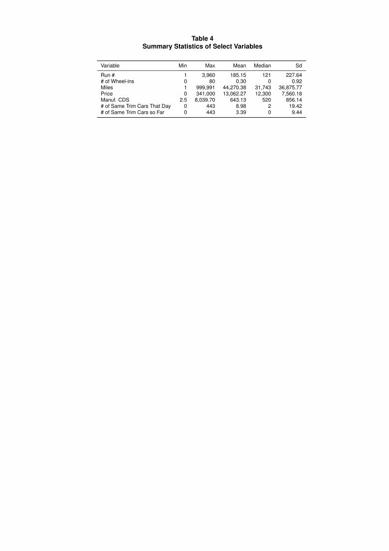
Table 4Summary Statistics of Select Variables
Variable Min Max Mean Median Sd
Run # 1 3,960 185.15 121 227.64# of Wheel-ins 0 80 0.30 0 0.92Miles 1 999,991 44,270.38 31,743 36,875.77Price 0 341,000 13,062.27 12,300 7,560.18Manuf. CDS 2.5 8,039.70 643.13 520 856.14# of Same Trim Cars That Day 0 443 8.98 2 19.42# of Same Trim Cars so Far 0 443 3.39 0 9.44

Table 5Car Prices and Manufacturer CDS by Car Condition
Condition Avg. Price Avg. Manuf. CDS
0 3,743.25 834.061 6,753.09 894.282 8,681.25 635.183 13,111.68 640.044 16,340.73 640.995 19,085.67 453.94

Table 6Car Prices and Manufacturer CDS by Mileage Bands
Mileage Band Avg. Mileage Avg. Price Avg. Manuf. CDS
1 4,818.98 19,823.08 614.322 10,244.34 17,936.70 649.723 13,244.71 17,111.88 625.504 15,880.88 16,573.01 609.785 18,459.50 16,143.92 603.336 20,856.87 15,730.07 616.697 23,214.74 15,149.07 627.938 25,765.59 14,497.46 638.189 28,215.15 13,917.72 701.23
10 30,416.64 13,901.36 691.4011 33,417.61 14,193.16 644.3612 37,167.25 14,303.58 591.9913 41,836.43 13,882.19 570.2914 47,083.13 13,417.75 553.9815 53,753.09 11,985.07 578.4516 62,320.51 10,172.16 616.9417 73,232.08 8,152.84 678.4418 87,090.39 6,365.74 719.1719 106,344.00 4,744.05 747.3920 152,056.50 3,242.93 783.55

Table 7Effect of Auto Manufacturers’ CDS Spread on Used Car Prices,
Baseline Specification
The dependent variable is the (raw or normalized) transacted price of the used cars in thesample. Manuf. CDS refers to the credit-default swap (CDS) spread (in basis points) of themanufacturers of the used cars. Manuf. CDS × Band 2-Band 20 denotes the interactionsof Manuf. CDS with a set of dummy variables indicating to which of the 20 mileage bandsa car belongs. Other controls not reported in the table include dummies for the auctionformat the car was sold under, the number of times the car was wheeled through the auctionlane, and the number of cars of the same model, trim and model year being sold on thesame day in the particular auction location. Columns (1) and (3) also include car conditioncontrols. All regressions include car type-region-week fixed effects. Reported standard errorsare clustered on car manufacturers×month, and are reported in parentheses (*** denotessignificance at the 1% level, ** at the 5% level, and * at the 10% level.)
(1) (2) (3) (4)
Dependent. Var: Price Normalized price Price Normalized price
Manuf. CDS -0.0679*** -6.07e-06*** -0.00514 -4.80e-06**(0.0214) (1.30e-06) (0.0340) (2.30e-06)
Manuf. CDS × Band 2 -0.0419* -4.19e-08(0.0233) (1.48e-06)
Manuf. CDS × Band 3 -0.0608** -5.68e-07(0.0250) (1.51e-06)
Manuf. CDS × Band 4 -0.0854*** -2.01e-06(0.0296) (1.71e-06)
Manuf. CDS × Band 5 -0.105*** -2.85e-06*(0.0322) (1.68e-06)
Manuf. CDS × Band 6 -0.119*** -3.44e-06*(0.0350) (1.83e-06)
Manuf. CDS × Band 7 -0.128*** -3.79e-06**(0.0338) (1.60e-06)
Manuf. CDS × Band 8 -0.143*** -4.65e-06**(0.0382) (1.90e-06)
Manuf. CDS × Band 9 -0.149*** -5.42e-06***(0.0360) (1.77e-06)
Manuf. CDS × Band 10 -0.147*** -5.33e-06***(0.0381) (1.56e-06)
Manuf. CDS Band 11 -0.120*** -4.10e-06***(0.0333) (1.38e-06)
Manuf. CDS × Band 12 -0.132*** -5.40e-06***(0.0296) (1.47e-06)
Manuf. CDS × Band 13 -0.108*** -6.15e-06***(0.0324) (1.96e-06)
Manuf. CDS × Band 14 -0.0811** -6.93e-06***(0.0350) (2.55e-06)
Manuf. CDS × Band 15 -0.00877 -5.60e-06(0.0427) (3.90e-06)
Manuf. CDS × Band 16 0.0429 -3.29e-06(0.0420) (5.35e-06)
Manuf. CDS × Band 17 0.107** 3.58e-06(0.0450) (6.23e-06)
Manuf. CDS × Band 18 0.151*** 1.31e-05*(0.0466) (7.28e-06)
Manuf. CDS × Band 19 0.158*** 1.93e-05**(0.0482) (9.48e-06)
Manuf. CDS × Band 20 0.173*** 3.30e-05***(0.0469) (1.23e-05)
Constant 10,768*** 1.198*** 10,720*** 1.197***(142.5) (0.00317) (135.3) (0.00354)
Observations 6188759 6188725 6188759 6188725R-squared 0.986 0.883 0.986 0.883

Table 8Effect of Auto Manufacturers’ CDS Spread on Used Car Prices,
Instrumental Variables for CDS
The dependent variable is the transacted price of the used cars in the sample. Manuf. CDS refers tothe credit-default swap (CDS) spread (in basis points) of the manufacturers of the used cars. CDS isinstrumented using the interaction of CAFE standards with NY gas price in Column 1, firm dummiesinteracted with NY gas price in Column 2, exchange rate for euro and yen in Columns 3 and 4, euroand yen simultaneously in Column 5 and euro yen and NY gas price in Column 6. NY gas prices arefrom the New York Harbor Conventional Gasoline Regular Spot Price FOB (Dollars per Gallon) (datafrom the U.S. Energy Information Administration (EIA)). Exchange rates are given as unit of foreigncurrency per dollar (data from the Economic Research Division at the Federal Reserve Bank at St.Louis). Other controls not reported in the table include dummies for the auction format the car wassold under, the number of times the car was wheeled through the auction lane, and the number of carsof the same model, trim and model year being sold on the same day in the particular auction location.Instrumental variable implemented using control function. Reported standard errors are clustered oncar manufacturers×month, and are reported in parentheses (*** denotes significance at the 1% level,** at the 5% level, and * at the 10% level.)
(1) (2) (3) (4) (5) (6)
Dependent. var: Price Price Price Price Price Price
Manuf. CDS -1.210 -0.0861 -0.0299 -0.225 -0.161 -0.0945(4.806) (0.161) (0.305) (0.230) (0.175) (0.142)
Control: CAFE 1.113(4.815)
Control: Gas NY -0.0102(0.178)
Gas NY -63.61 31.07 36.17(370.2) (68.63) (60.30)
Control: Euro -0.0826(0.323)
Euro 152.3 807.7 653.0(1325) (1060) (1201)
Control: Yen 0.110(0.255)
Yen -8.673 -7.612 -1.127(7.355) (6.714) (6.757)
Control: Euro/Yen 0.0354(0.212)
Control: Euro/Yen/GasNY -0.00916(0.183)
Constant 16349*** 15416*** 15362*** 16581*** 15825*** 15057***(3903) (251.6) (822.4) (953.3) (726.2) (1083)
Observations 4,013,475 4,003,544 6,162,182 6,162,182 6,162,182 4,003,544R-squared 0.986 0.986 0.984 0.984 0.984 0.986
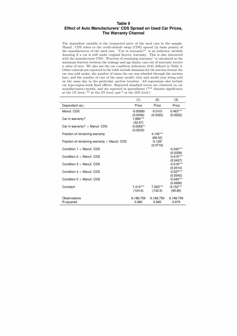
Table 9Effect of Auto Manufacturers’ CDS Spread on Used Car Prices,
The Warranty Channel
The dependent variable is the transacted price of the used cars in the sample.Manuf. CDS refers to the credit-default swap (CDS) spread (in basis points) ofthe manufacturers of the used cars. “Car in warranty?” is an indicator variabledenoting if a car is still under original factory warranty. This is also interactedwith the manufacturer CDS. “Fraction of remaining warranty” is calculated as theminimum fraction between the mileage and age limits; cars out of warranty receivea value of zero. We also use the car condition indicators (0-6) defined in Table 2.Other controls not reported in the table include dummies for the auction format thecar was sold under, the number of times the car was wheeled through the auctionlane, and the number of cars of the same model, trim and model year being soldon the same day in the particular auction location. All regressions also includecar type-region-week fixed effects. Reported standard errors are clustered on carmanufacturers×month, and are reported in parentheses (*** denotes significanceat the 1% level, ** at the 5% level, and * at the 10% level.)
(1) (2) (3)
Dependent var.: Price Price Price
Manuf. CDS -0.00580 -0.0101 0.463***(0.0246) (0.0322) (0.0522)
Car in warranty? 1,890***(32.67)
Car in warranty? × Manuf. CDS -0.0565**(0.0233)
Fraction of remaining warranty 4,145***(89.42)
Fraction of remaining warranty × Manuf. CDS -0.129*(0.0716)
Condition 1 × Manuf. CDS -0.342***(0.0358)
Condition 2 × Manuf. CDS -0.415***(0.0437)
Condition 3 × Manuf. CDS -0.518***(0.0510)
Condition 4 × Manuf. CDS -0.527***(0.0542)
Condition 5 × Manuf. CDS -0.540***(0.0690)
Constant 7,414*** 7,283*** 8,152***(124.9) (132.5) (99.80)
Observations 6,188,759 6,188,759 6,188,759R-squared 0.982 0.982 0.979

Table 10Effect of Auto Manufacturers’ CDS Spread on Used Car Prices: Parametric Mileage
(1) (2) (3) (4) (5)
Dependent var.: Price Price Price Price Price
Manuf. CDS -0.206*** -0.162*** -0.0997*** -0.0352 0.0487(0.0368) (0.0319) (0.0305) (0.0284) (0.0321)
Mileage × Manuf. CDS 0.0383*** 0.0211* -0.0197 -0.0725*** -0.154***(0.0123) (0.0109) (0.0140) (0.0195) (0.0314)
Mileage2× Manuf. CDS -0.000389 0.000881 0.00689*** 0.0175*** 0.0388***(0.000664) (0.000628) (0.00155) (0.00337) (0.00738)
Mileage3× Manuf. CDS -2.85e-05*** -0.000283*** -0.000977*** -0.00300***(1.09e-05) (6.28e-05) (0.000197) (0.000623)
Mileage4× Manuf. CDS 2.58e-06*** 1.78e-05*** 9.47e-05***(6.35e-07) (3.83e-06) (2.14e-05)
Mileage5× Manuf. CDS -1.01e-07*** -1.25e-06***(2.37e-08) (2.99e-07)
Mileage6× Manuf. CDS 5.79e-09***(1.45e-09)
Constant 11327*** 11535*** 11506*** 11350*** 11119***(143.5) (143.6) (145.1) (146.2) (145.0)
Observations 6188759 6188759 6188759 6188759 6188759R-squared 0.986 0.986 0.986 0.986 0.986
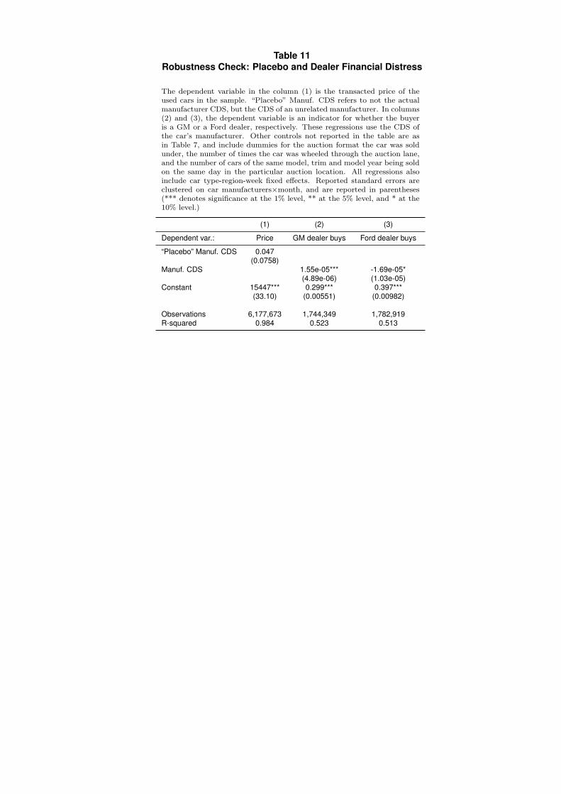
Table 11Robustness Check: Placebo and Dealer Financial Distress
The dependent variable in the column (1) is the transacted price of theused cars in the sample. “Placebo” Manuf. CDS refers to not the actualmanufacturer CDS, but the CDS of an unrelated manufacturer. In columns(2) and (3), the dependent variable is an indicator for whether the buyeris a GM or a Ford dealer, respectively. These regressions use the CDS ofthe car’s manufacturer. Other controls not reported in the table are asin Table 7, and include dummies for the auction format the car was soldunder, the number of times the car was wheeled through the auction lane,and the number of cars of the same model, trim and model year being soldon the same day in the particular auction location. All regressions alsoinclude car type-region-week fixed effects. Reported standard errors areclustered on car manufacturers×month, and are reported in parentheses(*** denotes significance at the 1% level, ** at the 5% level, and * at the10% level.)
(1) (2) (3)
Dependent var.: Price GM dealer buys Ford dealer buys
“Placebo” Manuf. CDS 0.047(0.0758)
Manuf. CDS 1.55e-05*** -1.69e-05*(4.89e-06) (1.03e-05)
Constant 15447*** 0.299*** 0.397***(33.10) (0.00551) (0.00982)
Observations 6,177,673 1,744,349 1,782,919R-squared 0.984 0.523 0.513

Table 12Robustness Check: Controlling for New Car Prices
Columns (2) and (3) of this table replicate Columns (1) and (2) of Table 9, butcontrolling for the new car price on the day of the auction (note that sample sizeis much smaller as we could not find new car transaction data for many auctiondays). Column (1) estimates the main effect of manufacturer CDS. As in Table 9,the dependent variable is the transacted price of the used cars in the sample.Manuf. CDS refers to the credit-default swap (CDS) spread (in basis points) ofthe manufacturers of the used cars. “Car in warranty?” is an indicator variabledenoting if a car is still under original factory warranty. This is also interactedwith the manufacturer CDS. “Fraction of remaining warranty” is calculated asthe minimum fraction between the mileage and age limits; cars out of warrantyreceive a value of zero. Other controls not reported in the table include dummiesfor the auction format the car was sold under, the number of times the car waswheeled through the auction lane, and the number of cars of the same model, trimand model year being sold on the same day in the particular auction location.All regressions also include car type-region-week fixed effects. Reported standarderrors are clustered on car manufacturers×month, and are reported in parentheses(*** denotes significance at the 1% level, ** at the 5% level, and * at the 10%level.)
(1) (2) (3)
Dependent var.: Price Price Price
Manuf. CDS -0.0775 0.0843 0.0677(0.0599) (0.0647) (0.0572)
Car in warranty? 2038***(50.28)
Car in warranty? × Manuf. CDS -0.135***(0.0326)
Fraction of remaining warranty 4721***(134.6)
Fraction of remaining warranty × Manuf. CDS -0.333**(0.152)
New car price -0.0019 -0.0023 -0.0018(0.0032) (0.0033) (0.0033)
Constant 17,102*** 13,337*** 13,333***(88.47) (83.34) (78.52)
Observations 1,007,990 1,007,990 1,007,990R-squared 0.980 0.975 0.977
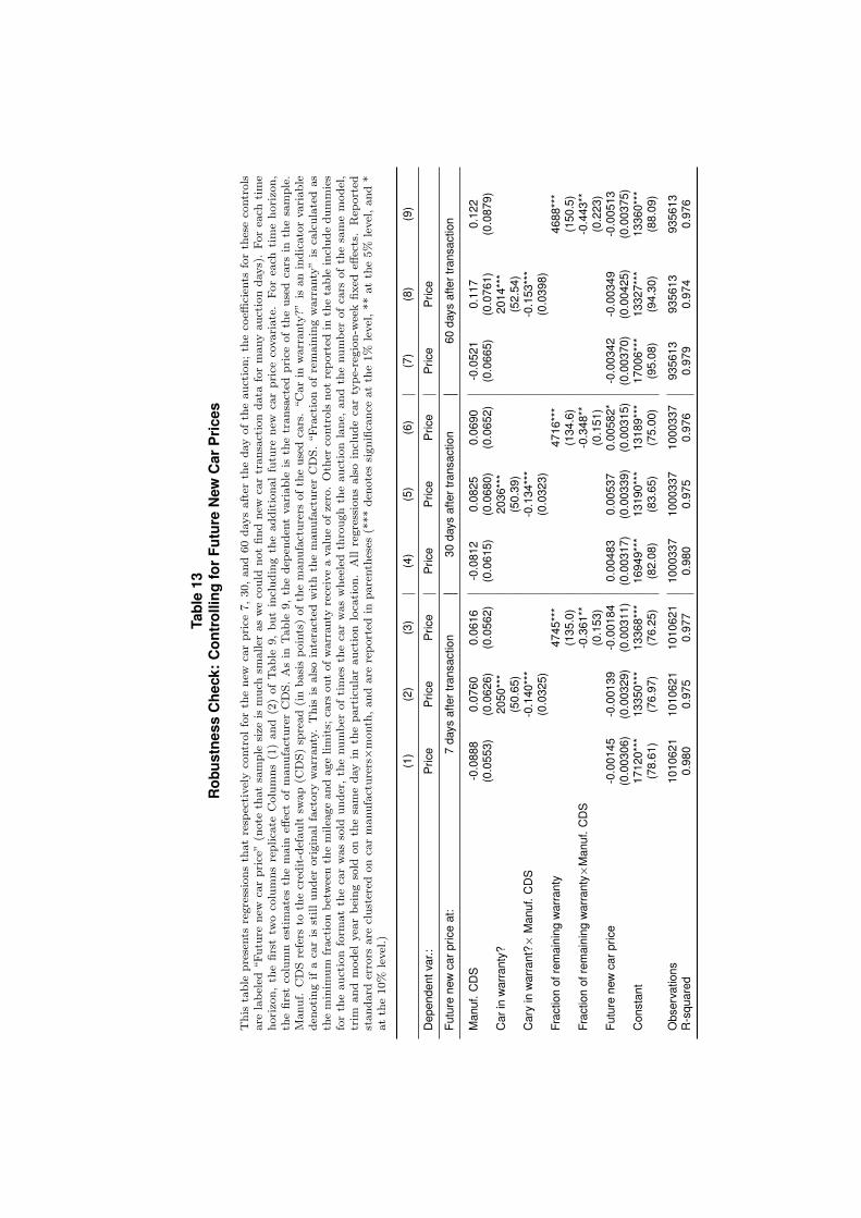
Tabl
e13
Rob
ustn
ess
Che
ck:
Con
trol
ling
for
Futu
reN
ewC
arP
rice
s
This
table
presents
regressionsth
atresp
ectivelyco
ntrolforth
enew
carprice
7,30,and60daysafter
thedayofth
eauction;th
eco
efficien
tsforth
eseco
ntrols
are
labeled
“Futu
renew
carprice”(n
ote
thatsample
size
ismuch
smaller
asweco
uld
notfindnew
cartransactiondata
formanyauctiondays).Forea
chtime
horizo
n,th
efirsttw
oco
lumnsreplica
teColumns(1)and
(2)ofTable
9,butincludingth
eadditionalfutu
renew
carprice
covariate.Forea
chtimehorizo
n,
thefirstco
lumnestimatesth
emain
effectofmanufacturerCDS.Asin
Table
9,th
edep
enden
tvariable
isth
etransacted
price
ofth
eusedca
rsin
thesample.
Manuf.
CDSrefers
toth
ecred
it-default
swap(C
DS)sp
read(inbasispoints)ofth
emanufacturers
ofth
eusedca
rs.“Carin
warranty?”is
anindicatorvariable
den
otingifaca
ris
stillunder
originalfactory
warranty.This
isalsointeracted
withth
emanufacturerCDS.“Fractionofremainingwarranty”is
calculatedas
theminim
um
fractionbetweenth
emilea
geandagelimits;
cars
outofwarranty
receiveavalueofzero.Oth
erco
ntrols
notreported
inth
etable
includedummies
forth
eauctionform
atth
eca
rwassold
under,th
enumber
oftimes
theca
rwaswheeledth
roughth
eauctionlane,
andth
enumber
ofca
rsofth
esamemodel,
trim
and
model
yea
rbeingsold
on
thesamedayin
theparticularauction
loca
tion.All
regressionsalsoincludeca
rtype-region-w
eekfixed
effects.Rep
orted
standard
errors
are
clustered
onca
rmanufacturers×month
,andare
reported
inparenth
eses
(***den
otessignifica
nce
atth
e1%
level,**atth
e5%
level,and*
atth
e10%
level.)
(1)
(2)
(3)
(4)
(5)
(6)
(7)
(8)
(9)
Dep
ende
ntva
r.:P
rice
Pric
eP
rice
Pric
eP
rice
Pric
eP
rice
Pric
e
Futu
rene
wca
rpric
eat
:7
days
afte
rtra
nsac
tion
30da
ysaf
tert
rans
actio
n60
days
afte
rtra
nsac
tion
Man
uf.
CD
S-0
.088
80.
0760
0.06
16-0
.081
20.
0825
0.06
90-0
.052
10.
117
0.12
2(0
.055
3)(0
.062
6)(0
.056
2)(0
.061
5)(0
.068
0)(0
.065
2)(0
.066
5)(0
.076
1)(0
.087
9)C
arin
war
rant
y?20
50**
*20
36**
*20
14**
*(5
0.65
)(5
0.39
)(5
2.54
)C
ary
inw
arra
nt?×
Man
uf.
CD
S-0
.140
***
-0.1
34**
*-0
.153
***
(0.0
325)
(0.0
323)
(0.0
398)
Frac
tion
ofre
mai
ning
war
rant
y47
45**
*47
16**
*46
88**
*(1
35.0
)(1
34.6
)(1
50.5
)Fr
actio
nof
rem
aini
ngw
arra
nty×
Man
uf.
CD
S-0
.361
**-0
.348
**-0
.443
**(0
.153
)(0
.151
)(0
.223
)Fu
ture
new
carp
rice
-0.0
0145
-0.0
0139
-0.0
0184
0.00
483
0.00
537
0.00
582*
-0.0
0342
-0.0
0349
-0.0
0513
(0.0
0306
)(0
.003
29)
(0.0
0311
)(0
.003
17)
(0.0
0339
)(0
.003
15)
(0.0
0370
)(0
.004
25)
(0.0
0375
)C
onst
ant
1712
0***
1335
0***
1336
8***
1694
9***
1319
0***
1318
9***
1700
6***
1332
7***
1336
0***
(78.
61)
(76.
97)
(76.
25)
(82.
08)
(83.
65)
(75.
00)
(95.
08)
(94.
30)
(88.
09)
Obs
erva
tions
1010
621
1010
621
1010
621
1000
337
1000
337
1000
337
9356
1393
5613
9356
13R
-squ
ared
0.98
00.
975
0.97
70.
980
0.97
50.
976
0.97
90.
974
0.97
6

Table 14Robustness Check: Controlling for Recalls
The dependent variable is the transacted price of the used cars in the sample.Manuf. CDS refers to the credit-default swap (CDS) spread (in basis points) ofthe manufacturers of the used cars. Recalls is the number of recalls of cars madeby each manufacturer on the transaction day. Car in warranty? is an indicatorvariable denoting if a car is still under original factory warranty. This is also in-teracted with the manufacturer CDS. Fraction of remaining warranty is calculatedas the minimum fraction between the mileage and age limits; cars out of warrantyreceive a value of zero. Other controls not reported in the table include dummiesfor the auction format the car was sold under, the number of times the car waswheeled through the auction lane, and the number of cars of the same model, trimand model year being sold on the same day in the particular auction location.All regressions also include car type-region-week fixed effects. Reported standarderrors are clustered on car manufacturers×month, and are reported in parentheses(*** denotes significance at the 1% level, ** at the 5% level, and * at the 10%level.)
(1) (2) (3)
Dependent var.: Price Price Price
Manuf. CDS -0.0736*** -0.00880 -0.0149(0.0210) (0.0269) (0.0323)
Car in warranty? 1954***(32.49)
Car in warrany? × Manuf. CDS -0.0563**(0.0252)
Recalls 4.28e-05 7.91e-05 5.23e-05(4.66e-05) (6.65e-05) (7.79e-05)
Fraction of remaining warranty 4236***(92.76)
Fraction of remaining warranty × Manuf. CDS -0.132*(0.0767)
Constant 15501*** 11868*** 11969***(35.88) (23.88) (28.81)
Observations 6188759 6188759 6188759R-squared 0.984 0.980 0.980

Tabl
e15
Rob
ustn
ess
Che
ck:
Con
trol
ling
for
Man
ufac
ture
rN
ews
Men
tion
Thedep
enden
tvariable
isth
etransacted
price
ofth
eusedca
rsin
thesample.Manuf.
CDSrefers
toth
ecred
it-default
swap(C
DS)sp
read(inbasispoints)ofth
emanufacturers
ofth
eused
cars.New
smen
tionsis
avariable
withmea
ningssp
ecificto
each
regressionset.
Allresu
lts((1),
(2),
(3))
counts
allarticlesth
atmen
tionagiven
automaker.Hea
dline((4),
(5),
(6))
counts
articlesth
atmen
tion
an
automaker
inth
ehea
dline.
Bankru
ptdistress((7),
(8),
(9))
counts
articlesth
atmen
tion
theautomaker
and
eith
er”bankru
pt”
(or”bankru
ptcy”)and
”distress”.
Recall((10),
(11),
(12))
counts
articlesth
atmen
tionth
eautomaker
and”reca
ll”.Carin
warranty?is
anindicatorvariable
den
otingifaca
ris
stillunder
originalfactory
warranty.This
isalso
interacted
withth
emanufacturerCDS.Fractionofremainingwarranty
isca
lculatedasth
eminim
um
fractionbetweenth
emilea
geandagelimits;
cars
outofwarranty
receiveavalueofzero.
Oth
erco
ntrols
notreported
inth
etable
includedummiesforth
eauctionform
atth
eca
rwassold
under,th
enumber
oftimes
theca
rwaswheeledth
roughth
eauctionlane,
andth
enumber
of
cars
ofth
esamemodel,trim
andmodel
yea
rbeingsold
onth
esamedayin
theparticularauctionloca
tion.Allregressionsalsoincludeca
rtype-region-w
eekfixed
effects.Allregressionsalso
includeca
rtype-region-w
eekfixed
effects.Rep
orted
standard
errors
are
clustered
onca
rmanufacturers×month
,andare
reported
inparenth
eses
(***den
otessignifica
nce
atth
e1%
level,**
atth
e5%
level,and*atth
e10%
level.)
(1)
(2)
(3)
(4)
(5)
(6)
(7)
(8)
(9)
(10)
(11)
(12)
Dep
ende
ntva
r.:P
rice
Pric
eP
rice
Pric
eP
rice
Pric
eP
rice
Pric
eP
rice
Pric
eP
rice
Pric
e
All
Res
ults
Hea
dlin
eB
ankr
uptd
istre
ssR
ecal
ls
Man
uf.
CD
S-0
.074
5***
-0.0
0621
-0.0
117
-0.0
738*
**-0
.006
46-0
.011
9-0
.078
8***
-0.0
105
-0.0
151
-0.0
740*
**-0
.006
88-0
.012
5(0
.021
4)(0
.027
4)(0
.033
3)(0
.021
2)(0
.027
2)(0
.033
2)(0
.020
3)(0
.027
0)(0
.033
6)(0
.021
1)(0
.027
1)(0
.033
0)C
arin
war
rant
y?19
59**
*19
59**
*19
59**
*19
59**
*(3
3.37
)(3
3.36
)(3
3.36
)(3
3.37
)C
arin
war
rant
y?×
Man
uf.
CD
S-0
.059
9**
-0.0
599*
*-0
.059
9**
-0.0
599*
*(0
.025
4)(0
.025
4)(0
.025
4)(0
.025
4)N
ews
Men
tions
-0.2
620.
132
0.08
53-0
.137
-0.7
63-0
.356
-3.2
17*
-2.5
83-2
.039
0.85
02.
374
3.84
2(0
.417
)(0
.433
)(0
.414
)(1
.579
)(1
.593
)(1
.619
)(1
.866
)(2
.256
)(2
.650
)(4
.429
)(4
.616
)(5
.107
)Fr
actio
nof
rem
aini
ngw
arra
nty
4254
***
4254
***
4254
***
4254
***
(96.
50)
(96.
50)
(96.
50)
(96.
49)
Frac
tion
ofre
mai
ning
war
rant
y×
Man
uf.
CD
S-0
.143
*-0
.143
*-0
.143
*-0
.143
*(0
.080
1)(0
.080
1)(0
.080
1)(0
.080
1)C
onst
ant
1567
6***
1201
0***
1213
4***
1567
3***
1201
3***
1213
5***
1567
8***
1201
6***
1213
8***
1567
3***
1201
1***
1213
4***
(37.
55)
(24.
98)
(30.
10)
(37.
75)
(24.
46)
(29.
58)
(37.
67)
(24.
36)
(29.
67)
(37.
67)
(24.
30)
(29.
24)
Obs
erva
tions
5926
446
5926
446
5926
446
5926
446
5926
446
5926
446
5926
446
5926
446
5926
446
5926
446
5926
446
5926
446
R-s
quar
ed0.
984
0.98
00.
980
0.98
40.
980
0.98
00.
984
0.98
00.
980
0.98
40.
980
0.98
0

Figure 1The panels compare the relative average used car prices and CDS series for Ford (top) and GM (bottom). Each series shows
the difference between the appropriate Ford (GM) series and the corresponding series for Honda. The price series are
constructed by taking the residual from a regression of cars’ auction prices on detailed car type fixed effects, sets of dummies
for mileage quantiles, auction location fixed effects, and week-of-year fixed effects. These residuals are averaged by week for
every manufacturer, and the difference between Ford’s (GM’s) and Honda’s price series is shown, after smoothing using a
12-week moving average, in the figure. The CDS series are computed by taking the car-weighted average CDS value for each
manufacturer and subtracting Honda’s series from Ford’s (GM’s). The log of this difference is shown in the figure to make
visualization easier.
!"#$%&
!"#$&
!"#"%&
"&
"#"%&
"#$&
"&
$&
'&
(&
)&
%&
*&
+&
,&
-&
$& *& $$& $*& '$& '*& ($& (*& )$& )*& %$& %*& *$& **& +$& +*& ,$& ,*& -$& -*&$"$&$"*&$$$&$$*&$'$&$'*&$($&$(*&$)$&$)*&!""#$%!""#$&'$()$*+,-+./$01123$
!"#$%&
!"#$&
!"#"%&
"&
"#"%&
"#$&
"&
$&
'&
(&
)&
%&
*&
+&
,&
-&
$& *& $$& $*& '$& '*& ($& (*& )$& )*& %$& %*& *$& **& +$& +*& ,$& ,*& -$& -*&$"$&$"*&$$$&$$*&$'$&$'*&$($&$(*&$)$&$)*&!""#$%!""#$&'$()$*+,-+./$01123$
(a) Ford
!"#$%&
!"#$&
!"#"'&
!"#"(&
!"#")&
!"#"%&
"&
"#"%&
"#")&
"#"(&
"#"'&
"&
$&
%&
*&
)&
+&
(&
,&
'&
-&
$"&
$& +& -& $*& $,& %$& %+& %-& **& *,& )$& )+& )-& +*& +,& ($& (+& (-& ,*& ,,& '$& '+& '-& -*& -,&$"$&$"+&$"-&$$*&$$,&$%$&$%+&$%-&$**&$*,&$)$&$)+&$)-&
!""#$%!""#$&'$()$*+,-+./$01123$
!"#$%&
!"#$&
!"#"'&
!"#"(&
!"#")&
!"#"%&
"&
"#"%&
"#")&
"#"(&
"#"'&
"&
$&
%&
*&
)&
+&
(&
,&
'&
-&
$"&
$& +& -& $*& $,& %$& %+& %-& **& *,& )$& )+& )-& +*& +,& ($& (+& (-& ,*& ,,& '$& '+& '-& -*& -,&$"$&$"+&$"-&$$*&$$,&$%$&$%+&$%-&$**&$*,&$)$&$)+&$)-&
!""#$%!""#$&'$()$*+,-+./$01123$
(b) GM

Figure 2Illustrative Figures of Used Car Auctions
(a) Auction Site (b) Inside an Auction
(c) The Auction Online

Figure 3Auto Manufacturer CDS Spreads
020
0040
0060
0080
00M
anuf
actu
rer
CD
S S
prea
d
01jan2006
01jan2007
01jan2008
01jan2009
Date
General Motors Corporation
010
0020
0030
0040
0050
00M
anuf
actu
rer
CD
S S
prea
d
01jan2006
01jan2007
01jan2008
01jan2009
Date
Ford Motor Company0
5010
015
0M
anuf
actu
rer
CD
S S
prea
d
01jan2006
01jan2007
01jan2008
01jan2009
Date
Toyota Motor Corporation
050
100
150
Man
ufac
ture
r C
DS
Spr
ead
01jan2006
01jan2007
01jan2008
01jan2009
Date
Honda Motor Company

Figure 4Plot of Mileage Interaction Coefficients from Column (3) of Table 7
Main effect
−.2
−.1
0.1
.2E
ffect
of m
anuf
. CD
S o
n us
ed c
ar p
rices
0 50000 100000 150000Mean car mileage within mileage band
Main effect + Mileage interactions 95% Confidence region

Figure 5Predicted CDS Effect on Price
−.2
−.1
0.1
.2.3
CD
S_2
0 50000 100000 150000Miles
−.2
−.1
0.1
.2.3
CD
S_3
0 50000 100000 150000Miles
−.1
0.1
.2.3
CD
S_4
0 50000 100000 150000Miles
−.1
0.1
.2.3
CD
S_5
0 50000 100000 150000Miles
−.1
0.1
.2.3
CD
S_6
0 50000 100000 150000Miles

Tabl
eA
1R
obus
tnes
sC
heck
:C
ontr
ollin
gfo
rLa
gged
Rec
alls
Thedep
enden
tvariable
isth
etransacted
price
ofth
eusedca
rsin
thesample.Manuf.
CDSrefers
toth
ecred
it-default
swap(C
DS)sp
read(inbasispoints)ofth
emanufacturers
ofth
eused
cars.Lagged
reca
llsis
thenumber
ofreca
llsofca
rsmadebyea
chmanufacturer1,7,30,and60daysbefore
thetransactionday,
resp
ectively.
Carin
warranty?is
anindicatorvariable
den
oting
ifaca
ris
stillunder
originalfactory
warranty.This
isalsointeracted
withth
emanufacturerCDS.Fractionofremainingwarranty
isca
lculatedasth
eminim
um
fractionbetweenth
emilea
ge
andagelimits;
cars
outofwarranty
receiveavalueofzero.Oth
erco
ntrols
notreported
inth
etable
includedummiesforth
eauctionform
atth
eca
rwassold
under,th
enumber
oftimes
the
carwaswheeledth
roughth
eauctionlane,
andth
enumber
ofca
rsofth
esamemodel,trim
andmodel
yea
rbeingsold
onth
esamedayin
theparticularauctionloca
tion.Allregressionsalso
includeca
rtype-region-w
eekfixed
effects.Rep
orted
standard
errors
are
clustered
onca
rmanufacturers×month
,andare
reported
inparenth
eses
(***den
otessignifica
nce
atth
e1%
level,**
atth
e5%
level,and*atth
e10%
level.)
(1)
(2)
(3)
(4)
(5)
(6)
(7)
(8)
(9)
(10)
(11)
(12)
Dep
eden
tvar
.:P
rice
Pric
eP
rice
Pric
eP
rice
Pric
eP
rice
Pric
eP
rice
Pric
eP
rice
Pric
e
1da
ybe
fore
trans
actio
n7
days
befo
retra
nsac
tion
30da
ysbe
fore
trans
actio
n60
days
befo
retra
nsac
tion
Man
uf.
CD
S-0
.073
8***
-0.0
0930
-0.0
152
-0.0
740*
**-0
.009
76-0
.015
6-0
.074
2***
-0.0
111
-0.0
174
-0.0
908*
**-0
.020
2-0
.026
4(0
.021
2)(0
.026
9)(0
.032
4)-0
.021
2-0
.026
9-0
.032
3-0
.021
2-0
.026
8-0
.031
5-0
.032
4-0
.030
8-0
.034
7C
arin
war
rant
y?19
54**
*19
53**
*19
51**
*19
47**
*(3
2.49
)-3
2.52
-33.
01-3
3.7
Car
inw
arra
nty?
×M
anuf
.C
DS
-0.0
563*
*-0
.055
5**
-0.0
543*
*-0
.052
1**
(0.0
252)
-0.0
253
-0.0
255
-0.0
258
Lagg
edR
ecal
ls8.
64e-
05*
5.98
e-05
7.00
e-05
-4.9
2E-0
5-9
.69E
-06
-1.0
2E-0
5-5
.15E
-05
-3.3
9E-0
5-4
.59E
-05
-5.2
7E-0
5-2
.41E
-05
-2.3
6E-0
5(4
.56e
-05)
(6.9
3e-0
5)(5
.48e
-05)
-0.0
0011
-8.0
6E-0
5-8
.76E
-05
-9.8
4E-0
5-0
.000
1-9
.98E
-05
-4.4
7E-0
5-3
.47E
-05
-3.7
2E-0
5Fr
actio
nof
rem
aini
ngw
arra
nty
4236
***
4236
***
4248
***
4260
***
(92.
76)
-92.
88-9
4.09
-96.
23Fr
actio
nof
rem
aini
ngw
arra
nty×
Man
uf.
CD
S-0
.132
*-0
.129
*-0
.126
*-0
.122
*(0
.076
7)-0
.075
5-0
.073
3-0
.070
9C
onst
ant
1550
1***
1186
8***
1196
9***
1550
3***
1187
0***
1197
0***
1552
7***
1188
6***
1198
1***
1555
9***
1190
5***
1199
4***
(35.
95)
(23.
88)
(28.
79)
-36
-23.
89-2
8.84
-36.
35-2
4.1
-29.
03-3
9.56
-26.
44-3
1.02
Obs
erva
tions
6188
759
6188
759
6188
759
6153
996
6153
996
6153
996
5998
937
5998
937
5998
937
5768
892
5768
892
5768
892
R-s
quar
ed0.
984
0.98
00.
980
0.98
40.
980.
980.
984
0.98
0.98
0.98
40.
980.
98

Tabl
eA
2R
obus
tnes
sC
heck
:C
ontr
ollin
gfo
rFu
ture
Rec
alls
Thedep
enden
tvariable
isth
etransacted
price
ofth
eusedca
rsin
thesample.Manuf.
CDSrefers
toth
ecred
it-default
swap(C
DS)sp
read(inbasispoints)ofth
emanufacturers
ofth
eused
cars.Futu
rereca
llsis
thenumber
ofreca
llsofca
rsmadebyea
chmanufactureron
1,7,30,and
60daysafter
thetransaction
day,
resp
ectively.
Carin
warranty?is
an
indicatorvariable
den
otingif
aca
ris
stillunder
originalfactory
warranty.This
isalsointeracted
withth
emanufacturerCDS.Fractionofremainingwarranty
isca
lculatedasth
eminim
um
fractionbetween
themilea
geandagelimits;
cars
outofwarranty
receiveavalueofzero.Oth
erco
ntrols
notreported
inth
etable
includedummiesforth
eauctionform
atth
eca
rwassold
under,th
enumber
oftimes
theca
rwaswheeledth
roughth
eauctionlane,
andth
enumber
ofca
rsofth
esamemodel,trim
andmodel
yea
rbeingsold
onth
esamedayin
theparticularauctionloca
tion.All
regressionsalsoincludeca
rtype-region-w
eekfixed
effects.Allregressionsalsoincludeca
rtype-region-w
eekfixed
effects.Rep
orted
standard
errors
are
clustered
onca
rmanufacturers×month
,andare
reported
inparenth
eses
(***den
otessignifica
nce
atth
e1%
level,**atth
e5%
level,and*atth
e10%
level.)
(1)
(2)
(3)
(4)
(5)
(6)
(7)
(8)
(9)
(10)
(11)
(12)
Dep
ende
ntva
r.:P
rice
Pric
eP
rice
Pric
eP
rice
Pric
eP
rice
Pric
eP
rice
Pric
eP
rice
Pric
e
1da
yaf
tert
rans
actio
n7
days
afte
rtra
nsac
tion
30da
ysaf
tert
rans
actio
n60
days
afte
rtra
nsac
tion
Man
uf.
CD
S-0
.073
6***
-0.0
0947
-0.0
154
-0.0
738*
**-0
.009
21-0
.015
2-0
.073
9***
-0.0
0933
-0.0
152
-0.0
819*
*-0
.008
25-0
.008
33(0
.021
0)(0
.026
9)(0
.032
4)(0
.021
2)(0
.026
9)(0
.032
4)(0
.021
2)(0
.026
9)(0
.032
4)(0
.033
6)(0
.039
4)(0
.049
0)C
arin
war
rant
y?19
54**
*19
54**
*19
54**
*19
57**
*(3
2.49
)(3
2.49
)(3
2.49
)(3
4.75
)C
arin
war
rant
y?×
Man
uf.
CD
S-0
.056
3**
-0.0
563*
*-0
.056
3**
-0.0
618*
(0.0
252)
(0.0
252)
(0.0
252)
(0.0
317)
Futu
reR
ecal
ls2.
14e-
05-1
.67e
-05
-1.8
7e-0
54.
53e-
057.
06e-
052.
60e-
05-1
.44e
-05
-1.3
7e-0
5-1
.93e
-06
5.83
e-05
5.07
e-05
2.20
e-05
(2.5
6e-0
5)(3
.35e
-05)
(2.7
0e-0
5)(7
.66e
-05)
(6.1
9e-0
5)(6
.78e
-05)
(2.5
3e-0
5)(2
.76e
-05)
(3.0
4e-0
5)(4
.39e
-05)
(3.5
4e-0
5)(3
.99e
-05)
Frac
tion
ofre
mai
ning
war
rant
y42
36**
*42
36**
*42
36**
*42
58**
*(9
2.76
)(9
2.76
)(9
2.76
)(1
04.3
)Fr
actio
nof
rem
aini
ngw
arra
nty×
Man
uf.
CD
S-0
.132
*-0
.132
*-0
.132
*-0
.184
(0.0
767)
(0.0
767)
(0.0
767)
(0.1
20)
Con
stan
t15
501*
**11
869*
**11
970*
**15
501*
**11
868*
**11
969*
**15
501*
**11
869*
**11
970*
**15
518*
**11
884*
**11
984*
**(3
5.89
)(2
3.85
)(2
8.79
)(3
6.02
)(2
3.88
)(2
8.82
)(3
5.93
)(2
3.88
)(2
8.80
)(3
9.42
)(2
8.74
)(3
4.81
)
Obs
erva
tions
6188
759
6188
759
6188
759
6188
759
6188
759
6188
759
6188
759
6188
759
6188
759
6103
801
6103
801
6103
801
R-s
quar
ed0.
984
0.98
00.
980
0.98
40.
980
0.98
00.
984
0.98
00.
980
0.98
40.
980
0.98
0

Table A3Robustness Check: Controlling for 3 Day Moving Average Recalls
The dependent variable is the transacted price of the used cars in the sample.Manuf. CDS refers to the credit-default swap (CDS) spread (in basis points) ofthe manufacturers of the used cars. Recalls 3DMA is a three day moving averagearound the transaction day of the number of recalls of cars made by each manu-facturer. Car in warranty? is an indicator variable denoting if a car is still underoriginal factory warranty. This is also interacted with the manufacturer CDS.Fraction of remaining warranty is calculated as the minimum fraction between themileage and age limits; cars out of warranty receive a value of zero. Other controlsnot reported in the table include dummies for the auction format the car was soldunder, the number of times the car was wheeled through the auction lane, and thenumber of cars of the same model, trim and model year being sold on the same dayin the particular auction location. All regressions also include car type-region-weekfixed effects. Reported standard errors are clustered on car manufacturers×month,and are reported in parentheses (*** denotes significance at the 1% level, ** at the5% level, and * at the 10% level.)
(1) (2) (3)Dependent var.: Price Price Price
Manuf. CDS -0.0729*** -0.00877 -0.0148(0.0208) (0.0270) (0.0325)
Car in warranty? 1954***(32.49)
Car in warranty? × Manuf. CDS -0.0563**(0.0252)
Recalls 3DMA 0.000173* 0.000102 8.45e-05(9.98e-05) (0.000114) (0.000104)
Fraction of warranty remaining 4236***(92.76)
Fraction of remaining warranty × Manuf. CDS -0.132*(0.0767)
Constant 15500*** 11868*** 11969***(35.90) (23.92) (28.87)
Observations 6188759 6188759 6188759R-squared 0.984 0.980 0.980