Embed Size (px)
Citation preview

ARCube: supporting ranking aggregate queries in partially materialized data cubes
SIGMOD 2008Tianyi Wu1 Dong Xin2 Jiawei Han1 1University of Illinois, Urbana-Champaign, Urbana, IL, USA 2Microsoft Research, Redmond, WA, USA
Presenter : Chun Kit Chui (Kit)Supervisor : Dr. Ben Kao

Outline
Introduction Traditional top-k queries Aggregate queries
What is AR-cube? The basic query execution framework using AR-cube Optimizations
Chunking Scheduling
Supporting general ranking functions SUM, MIN, MAX, STDEV, VAR, MAD, AVG
Experimental results
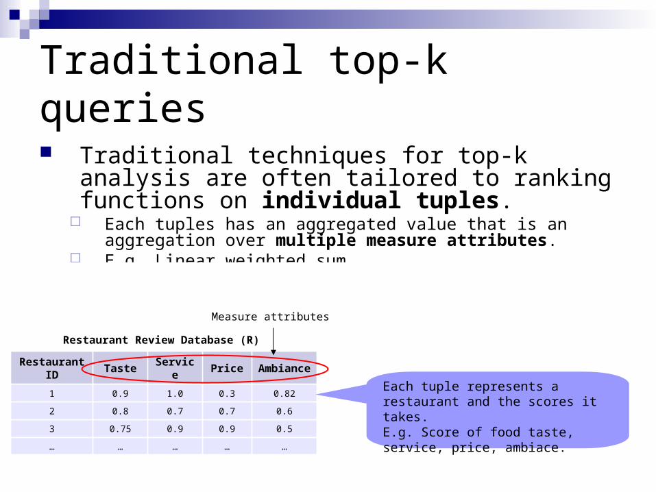
Traditional top-k queries
Traditional techniques for top-k analysis are often tailored to ranking functions on individual tuples.
Each tuples has an aggregated value that is an aggregation over multiple measure attributes.
E.g. Linear weighted sum
Restaurant ID
Taste Service Price AmbianceRanking function
1 0.9 1.0 0.3 0.82 0.73
2 0.8 0.7 0.7 0.6 0.664
3 0.75 0.9 0.9 0.5 0.81
… … … … … …
Restaurant Review Database (R)
Measure attributes
Each tuple represents a restaurant and the scores it takes.E.g. Score of food taste, service, price, ambiace.

Traditional top-k queries
Traditional techniques for top-k analysis are often tailored to ranking functions on individual tuples.
Each tuples has an aggregated value that is an aggregation over multiple measure attributes.
Example top-k query: To find the top rated restaurant according to a user specified ranking function.
Ranking function : Linear weighted sum
Restaurant ID
Taste Service Price AmbianceRanking function
1 0.9 1.0 0.3 0.82 0.73
2 0.8 0.7 0.7 0.6 0.664
3 0.75 0.9 0.9 0.5 0.81
… … … … … …
Example Top-k Query
SELECT *
FROM R
ORDER BY
Taste*0.6+Service*0.1+Price*0.3 desc
LIMIT 1
Restaurant Review Database (R)
Ranking function
The top-k parameter
Each tuple has its own ranking score. The top ranked tuple is returned to user.

Aggregate queries
ID Time Location Type Sales
1 2007 Chicago Sedan 13
2 2007 Chicago Pickup 12
3 2007 Vancouver SUV 10
4 2008 Vancouver Sedan 37
5 2008 Vancouver SUV 20
… … … … …
Car sales database (S) Dimension attributes Measure attribute
Each tuple shows the number of car sales of a particular time, location, and car type.
E.g. 13 Sedan cars were sold in Chicago in year 2007.

Aggregate queries
An aggregate query consist of 2 core parts Group by
Define on the dimension attributes Determine the dimension of the returned result (cuboid) Define the grouping of tuples : tuples that share the same values in those dimension
attributes are grouped together. Aggregate measure
Define on measure attributes Apply to the measure attributes of the records in each group. E.g. SUM,MIN,MAX,AVG, STDEV…etc
ID Time Location Type Sales
1 2007 Chicago Sedan 13
2 2007 Chicago Pickup 12
3 2007 Vancouver SUV 10
4 2008 Vancouver Sedan 37
5 2008 Vancouver SUV 20
… … … … …
Car sales database (S) Dimension attributes Measure attribute
Example Aggregate Query
SELECT Time, Location, SUMSUM(Sales)
FROM S
GROUP BY Time, Location
ORDER BY SUMSUM(Sales) desc
LIMIT 2We want to group the tuples according to the Time and Location attributes.
Time Location
Query result (2D cuboid)
Since there are two dimension attributes, the resulting cuboid is a 2-Dimensional summary.

Aggregate queries
An aggregate query consist of 2 core parts Group by
Define on the dimension attributes Determine the number of cells in the returned result (cuboid) Define the grouping of tuples : tuples that share the same values in those dimension
attributes are grouped together. Aggregate measure
Define on measure attributes Apply to the measure attributes of the records in each group. E.g. SUM,MIN,MAX,AVG, STDEV…etc
ID Time Location Type Sales
1 2007 Chicago Sedan 13
2 2007 Chicago Pickup 12
3 2007 Vancouver SUV 10
4 2008 Vancouver Sedan 37
5 2008 Vancouver SUV 20
… … … … …
Car sales database (S) Dimension attributes Measure attribute
Example Aggregate Query
SELECT Time, Location, SUMSUM(Sales)
FROM S
GROUP BY Time, Location
ORDER BY SUMSUM(Sales) desc
LIMIT 2
Time Location Tuples Sales
2007 Chicago 1,2 13+12=25
2007 Vancouver 3 10
2008 Vancouver 4,5 37+20=57
2008 Chicago ... …
… … …
Query result (2D cuboid)
If we consider the time from year 2000 to 2009 and 30 locations, then there will be 10*30=300 cells. The number of cells in the cuboid is exponential to the number of dimensions of the cuboid.

Aggregate queries
An aggregate query consist of 2 core parts Group by
Define on the dimension attributes Determine the number of cells in the returned result (cuboid) Define the grouping of tuples : tuples that share the same values in those dimension
attributes are grouped together. Aggregate measure
Define on measure attributes Apply to the measure attributes of the records in each group. E.g. SUM,MIN,MAX,AVG, STDEV…etc
ID Time Location Type Sales
1 2007 Chicago Sedan 13
2 2007 Chicago Pickup 12
3 2007 Vancouver SUV 10
4 2008 Vancouver Sedan 37
5 2008 Vancouver SUV 20
… … … … …
Car sales database (S) Dimension attributes Measure attribute
Example Aggregate Query
SELECT Time, Location, SUMSUM(Sales)
FROM S
GROUP BY Time, Location
ORDER BY SUMSUM(Sales) desc
LIMIT 2
Time Location Tuples Sales
2007 Chicago 1,2 13+12=25
2007 Vancouver 3 10
2008 Vancouver 4,5 37+20=57
2008 Chicago ... …
… … …
Query result (2D cuboid)

Aggregate queries
An aggregate query consist of 2 core parts Group by
Define on the dimension attributes Determine the number of cells in the returned result (cuboid) Define the grouping of tuples : tuples that share the same values in those dimension
attributes are grouped together. Aggregate measure
Define on measure attributes Apply to the measure attributes of the tuples in each group. E.g. SUM,MIN,MAX,AVG, STDEV…etc
ID Time Location Type Sales
1 2007 Chicago Sedan 13
2 2007 Chicago Pickup 12
3 2007 Vancouver SUV 10
4 2008 Vancouver Sedan 37
5 2008 Vancouver SUV 20
… … … … …
Car sales database (S) Dimension attributes Measure attribute
Example Aggregate Query
SELECT Time, Location, SUMSUM(Sales)
FROM S
GROUP BY Time, Location
ORDER BY SUMSUM(Sales) desc
LIMIT 2
Time Location Tuples SUM(Sale)
2007 Chicago 1,2 13+12=25
2007 Vancouver 3 10
2008 Vancouver 4,5 37+20=57
2008 Chicago ... …
… … …
Query result (2D cuboid)
The SUM aggregate measure is defined on the Sales attribute

Aggregate queries
ID Time Location Type Sales
1 2007 Chicago Sedan 13
2 2007 Chicago Pickup 12
3 2007 Vancouver SUV 10
4 2008 Vancouver Sedan 37
5 2008 Vancouver SUV 20
… … … … …
Car sales database (S) Dimension attributes Measure attribute
Example Aggregate Query
SELECT Time, Location, SUMSUM(Sales)
FROM S
GROUP BY Time, Location
ORDER BY SUMSUM(Sales) desc
LIMIT 2
Time Location Tuples SUM(Sale)
2007 Chicago 1,2 13+12=25
2007 Vancouver 3 10
2008 Vancouver 4,5 37+20=57
2008 Chicago ... …
… … …
Query result (2D cuboid)
The number of cuboid cells is exponential to the number of dimension attributes. When the dimensionality is high, the returned cuboid is often
gigantic (i.e. may cuboid cells) Inefficient to compute the full cuboid.

Aggregate queriesExample Top K Aggregate Query
SELECT Time, Location, SUMSUM(Sales)
FROM S
GROUP BY Time, Location
ORDER BY SUMSUM(Sales) desc
LIMIT 1
Time Location Tuples SUM(Sale)
2007 Chicago 1,2 13+12=25
2007 Vancouver 3 10
2008 Vancouver 4,5 37+20=57
2008 Chicago ... …
… … …
Query result (cuboid)
Top-k aggregate queries Return only the top-k ranked cells The presentation will be more comprehensible Computation is potentially more efficient
E.g. Instead of knowing the total number of car sales in each year and in each location, the manager would like to find in which year and in which location having the most number of car sales.

Contributions
Study the problem of Top-k aggregate queries processing.
Propose the Aggregate Ranking cube (AR-Cube) for supporting Top-k aggregate queries Novel partial cube Unified structure for supporting various aggregate measures
(e.g. SUM, MAX, MIN, AVG, RANGE, STDEV, VAR, MAD) Basic query execution algorithm
Thresholding technique I/O optimizations

Aggregate Ranking Cube (AR-cube)

Intuition Query: Find the Top-1 populated city in US. Naive approach : Find out the populations of all US cities, and then
sort them in descending order of their populations, and return the first city in the list.
The evaluation can be better if we have some more information to guide our search.
If the state population (i.e. higher level statistics) is known, then we can use the state population as a guide to our search for the top-1 populated city.
Basic intuition : We should search the city in the most populated states first.

Intuition By checking the cities in the top states, we found out that…
NYC: 8M LA: 4M Chicago: 3M
Since the state population is the maximal possible population of their cities, cities in the 39 states (in red) can be pruned because all cities in these states cannot have population over 8M (current top-1). California 36M Virginia 7M
Texas 23M Washington 6M
New York 19M Massachusetts 6M
Florida 18M Indiana 6M
Illinois 12M Arizona 6M
Pennsylvania 12M Tennessee 6M
Ohio 11M Missouri 5M
Michigan 10M Maryland 5M
Georgia 9M Wisconsin 5M
N. Carolina 9M Minnesota 5M
New Jersey 8M 29 more… <5M
PRUNED

Intuition
California 36M Virginia 7M
Texas 23M Washington 6M
New York 19M Massachusetts 6M
Florida 18M Indiana 6M
Illinois 12M Arizona 6M
Pennsylvania 12M Tennessee 6M
Ohio 11M Missouri 5M
Michigan 10M Maryland 5M
Georgia 9M Wisconsin 5M
N. Carolina 9M Minnesota 5M
New Jersey 8M 29 more… <5M
PRUNED
This example demonstrates that Some high level statistics can guide our search for
top-k results. Also, the current top-k values can help us to eliminate
a lot of candidates.

Aggregate-Ranking Cube (AR-Cube) AR-cube consists of
Guiding cuboids Store high-level statistics to guide the search of promising candidate
cells. Supporting cuboids
Verify the true aggregate values of the cuboid cells. It contains inverted index to support efficient online aggregation
Unified structure to support various aggregate measures Monotonic: SUM, COUNT, MAX, etc. Non-monotonic: AVG, STDDEV, RANGE, etc.

Guiding cuboid Tid A B C Score
T1 a1 b1 c3 63
T2 a1 b2 c1 10
T3 a1 b2 c3 50
T4 a2 b1 c3 16
T5 a2 b2 c1 52
T6 a3 b1 c1 35
T7 a3 b1 c2 40
T8 a3 b2 c1 45
A SUM
a1 123
a2 68
a3 120
Cgd(A,SUM)
Guiding measureGroup-by dimension attribute
Guiding cuboids store high-level statistics to guide the search of promising candidate cells.
To define a guiding cuboid, we need to specify:
Group by Defined on dimension attributes Determine the grouping of tuples.
Guiding measure Define on measure attribute Apply on the tuples in each group.
Database (S)
Since the group by is on attribute A, and there are 3 distinct values in attribute A, there are 3 cells in total.
The guiding measure is applied on the tuples in each group. T1, t2, t3 are in cell a1, so their scores are sum up and stored in this cell

Guiding cuboid Tid A B C Score
T1 a1 b1 c3 63
T2 a1 b2 c1 10
T3 a1 b2 c3 50
T4 a2 b1 c3 16
T5 a2 b2 c1 52
T6 a3 b1 c1 35
T7 a3 b1 c2 40
T8 a3 b2 c1 45
A SUM
a1 123
a2 68
a3 120
Cgd(A,SUM)
Guiding measureGroup-by dimension attribute
B SUM
b1 154
b2 157
Cgd(B,SUM)AB SUM
a1, b1 63
a1, b2 60
a2, b1 16
a2, b2 52
a3, b1 75
a3, b2 45
Cgd(AB,SUM)
Guiding cuboids store high-level statistics to guide the search of promising candidate cells
To define a guiding cuboid, we need to specify:
Group by Defined on dimension attributes Determine the grouping of tuples.
Guiding measure Define on measure attribute Apply on the tuples in each group.
Database (S)

Supporting cuboid Tid A B C Score
T1 a1 b1 c3 63
T2 a1 b2 c1 10
T3 a1 b2 c3 50
T4 a2 b1 c3 16
T5 a2 b2 c1 52
T6 a3 b1 c1 35
T7 a3 b1 c2 40
T8 a3 b2 c1 45
Database (S)
A Inverted index
a1 (t1,63), (t2, 10), (t3, 50)
a2 (t4, 16), (t5, 52)
a3 (t6, 35), (t7, 40), (t8, 45)
Csp(A)
B Inverted index
b1 (t1,63), (t4, 16), (t6, 35), (t7, 40)
b2 (t2, 10), (t3, 50), (t5, 52), (t8, 45)
Csp(B)
Supporting cuboids help verify the true aggregate values of the cuboid cells.
To define a supporting cuboid, we need to specify : Group by
Define on dimension attribute Determine the grouping of tuples.
Stores the raw values of the measure attribute. Each cuboid cell g contains the inverted index
of g.
Group-by dimension attribute

AR-cube
Given a set of group-by’s, A1,...,AD ,and a set of aggregate measures M
An AR-cube, C(A1,…,AD ; M) consists of D guiding cuboids Cgd(Ai,M), 1<=i<=D, and D supporting cuboids Csp(Ai).
A SUM
a1 123
a2 68
a3 120
Cgd(A,SUM)
B SUM
b1 154
b2 157
Cgd(B,SUM)
A Inverted index
a1 (t1,63), (t2, 10), (t3, 50)
a2 (t4, 16), (t5, 52)
a3 (t6, 35), (t7, 40), (t8, 45)
Csp(A)
B Inverted index
b1 (t1,63), (t4, 16), (t6, 35), (t7, 40)
b2 (t2, 10), (t3, 50), (t5, 52), (t8, 45)
Csp(B)
C (A,B;SUM)
Guiding cuboids Supporting cuboidsAR-cube

Query Execution Models

Motivating example
Query Top-1 cell Group-by (A,B) Aggregate measure: SUM
If Cgd(AB,SUM) is materialized, the answer can be returned very quickly.
Otherwise, we have to compute the result with the help of materialized guiding and supporting cuboids.
AB SUM
a1, b1 63
a1, b2 60
a2, b1 16
a2, b2 52
a3, b1 75
a3, b2 45
Cgd(AB,SUM)
Tid A B C Score
T1 a1 b1 c3 63
T2 a1 b2 c1 10
T3 a1 b2 c3 50
T4 a2 b1 c3 16
T5 a2 b2 c1 52
T6 a3 b1 c1 35
T7 a3 b1 c2 40
T8 a3 b2 c1 45
Database (S)

Motivating example
Query Top-1 cell Group-by (A,B) Aggregate measure: SUM
If Cgd(AB,SUM) is materialized, the answer can be returned very quickly.
Otherwise, we have to compute the result with the help of materialized guiding and supporting cuboids.
To compute the query with A,B as dimension attributes and SUM aggregate measure, we need the guiding cuboids with dimension attribute A and B and SUM guiding measure.A SUM
a1 123
a2 68
a3 120
Cgd(A,SUM)B SUM
b1 154
b2 157
Cgd(B,SUM)
Tid A B C Score
T1 a1 b1 c3 63
T2 a1 b2 c1 10
T3 a1 b2 c3 50
T4 a2 b1 c3 16
T5 a2 b2 c1 52
T6 a3 b1 c1 35
T7 a3 b1 c2 40
T8 a3 b2 c1 45
Database (S)

Query execution model
A SUM
a1 123
a2 68
a3 120
Cgd(A,SUM)B SUM
b1 154
b2 157
Cgd(B,SUM)
A candidate generation and verification framework Candidate generation
The most promising candidate is generated by considering the high level statistics (guiding cuboids).
Verification The true aggregate measure of the candidate is verified (supporting
cuboids). Update and pruning
Knowing the true aggregate measure of a candidate help us to refine the upper bound of other candidates
Sorted lists initialization
Sorted lists initialization
Candidategeneration
Candidategeneration VerificationVerification Update sorted lists
and pruning
Update sorted lists and pruning

Query execution model
A SUM
a1 123
a2 68
a3 120
Cgd(A,SUM)B SUM
b1 154
b2 157
Cgd(B,SUM)
Candidategeneration
Candidategeneration VerificationVerification Update sorted lists
and pruning
Update sorted lists and pruning
Step 1. Sorted lists initialization In this step, we initialize one sorted list for each guiding cuboid. The sorted lists tells
Largest aggregate a combined candidate cell could achieve (i.e., the aggregate bound of the cuboid cells)
e.g. a1=123 means that the aggregate measures of the unseen cells, with a1 as their value in attribute A, are upper bounded by 123.
Sorted lists initialization
Sorted lists initialization
A Bound
a1 123
a3 120
a2 68
B Bound
b2 157
b1 154
Sorted list A Sorted list B
Guiding cellsSince the aggregate bounds store in the cells of the sorted list will guide our search for the top-k candidates, we call the cells guiding cells.

Sorted lists initialization
Sorted lists initialization
Query execution model
A SUM
a1 123
a2 68
a3 120
Cgd(A,SUM)B SUM
b1 154
b2 157
Cgd(B,SUM)
VerificationVerification Update sorted lists and pruning
Update sorted lists and pruning
Step 2. Candidate generation Intuition of candidate generation: to generate the cell
that likely to have large aggregate value. Generate the cell according to the top entry of the
sorted lists. In this case, (a1,b2) is generated as the next promising
candidate cell.
A Bound
a1 123
a3 120
a2 68
B Bound
b2 157
b1 154
Sorted list A Sorted list B
Candidategeneration
Candidategeneration
b2
b1
a1 a2 a3

Sorted lists initialization
Sorted lists initialization
Query execution modelUpdate sorted lists
and pruning
Update sorted lists and pruning
Step 3. Verify the true aggregate value of the candidate cell We need to consult the supporting cuboids and fetch
the corresponding inverted-indices. Perform list intersection
We now know the true aggregate value of the cell (a1, b2) is 60. (a1,b2)=60 is the current top-1 aggregate measure.
A Bound
a1 123
a3 120
a2 68
B Bound
b2 157
b1 154
Sorted list A Sorted list B
Candidategeneration
Candidategeneration VerificationVerification
A Inverted index
a1 (t1,63), (t2, 10), (t3, 50)
a2 (t4, 16), (t5, 52)
a3 (t6, 35), (t7, 40), (t8, 45)
Csp(A)B Inverted index
b1 (t1,63), (t4, 16), (t6, 35), (t7, 40)
b2 (t2, 10), (t3, 50), (t5, 52), (t8, 45)
Csp(B)
60b2
b1
a1 a2 a3

Sorted lists initialization
Sorted lists initialization
Query execution model
Step 4. Update the sorted lists Since we now know that (a1,b2) = 60, we can refine the
aggregate bound of the unseen cells with a1 as their values in attribute A i.e. (a1, *) as 123-60 = 63.
Similarly we update the aggregate bound of the the sorted list B.
A Bound
a1 123-60
a3 120
a2 68
B Bound
b2 157-60
b1 154
Sorted list A Sorted list B
Candidategeneration
Candidategeneration VerificationVerification Update sorted lists
and pruning
Update sorted lists and pruning
A Bound
a3 120
a2 68
a1 63
B Bound
b1 154
b2 97
Sorted list A Sorted list B
Update
60b2
b1
a1 a2 a3
After the update, the order of entries in the sorted list is also updated

Sorted lists initialization
Sorted lists initialization
Query execution model
With the upper bound refined, we may use the current top-k threshold to prune some candidates Pruning conditions:
If the value of a cell in the sorted list is smaller than the threshold, then all combined candidates cannot have aggregate measure larger than the threshold and can be pruned.
If an entry in the sorted list is pruned, all the subsequent entries in the list can be pruned.
Candidategeneration
Candidategeneration VerificationVerification Update sorted lists
and pruning
Update sorted lists and pruning
A Bound
a3 120
a2 68
a1 63
B Bound
b1 154
b2 97
Sorted list A Sorted list B
60b2
b1
a1 a2 a3
In this case, none of the cells have value below 60, no cells can be pruned.

Update sorted lists and pruning
Update sorted lists and pruning
Sorted lists initialization
Sorted lists initialization
Query execution modelVerificationVerification
A Bound
a3 120
a2 68
a1 63
B Bound
b1 154
b2 97
Sorted list A Sorted list B
60b2
b1
a1 a2 a3
Candidategeneration
Candidategeneration
Generate the next promising candidate cell according to the first entry of the sorted lists. i.e. (a3, b1)

Update sorted lists and pruning
Update sorted lists and pruning
Sorted lists initialization
Sorted lists initialization
Query execution model
A Bound
a3 120
a2 68
a1 63
B Bound
b1 154
b2 97
Sorted list A Sorted list B
60
75
b2
b1
a1 a2 a3
Candidategeneration
Candidategeneration
A Inverted index
a1 (t1,63), (t2, 10), (t3, 50)
a2 (t4, 16), (t5, 52)
a3 (t6, 35), (t7, 40), (t8, 45)
Csp(A)B Inverted index
b1 (t1,63), (t4, 16), (t6, 35), (t7, 40)
b2 (t2, 10), (t3, 50), (t5, 52), (t8, 45)
Csp(B)
VerificationVerification
Retrieve the corresponding inverted indices from supporting cuboids and verify the true aggregate value of the candidate cell.

Sorted lists initialization
Sorted lists initialization
Query execution model
A Bound
a3 120-75
a2 68
a1 63
B Bound
b1 154-75
b2 97
Sorted list A Sorted list B
60
75
b2
b1
a1 a2 a3
Candidategeneration
Candidategeneration
A Inverted index
a1 (t1,63), (t2, 10), (t3, 50)
a2 (t4, 16), (t5, 52)
a3 (t6, 35), (t7, 40), (t8, 45)
Csp(A)B Inverted index
b1 (t1,63), (t4, 16), (t6, 35), (t7, 40)
b2 (t2, 10), (t3, 50), (t5, 52), (t8, 45)
Csp(B)
VerificationVerification Update sorted lists and pruning
Update sorted lists and pruning
A Bound
a2 68
a1 63
a3 45
B Bound
b2 97
b1 79
Sorted list A Sorted list B
Update
Refine the aggregate bounds.

Sorted lists initialization
Sorted lists initialization
Query execution model
A Bound
a3 120-75
a2 68
a1 63
B Bound
b1 154-75
b2 97
Sorted list A Sorted list B
60
75
b2
b1
a1 a2 a3
Candidategeneration
Candidategeneration
A Inverted index
a1 (t1,63), (t2, 10), (t3, 50)
a2 (t4, 16), (t5, 52)
a3 (t6, 35), (t7, 40), (t8, 45)
Csp(A)B Inverted index
b1 (t1,63), (t4, 16), (t6, 35), (t7, 40)
b2 (t2, 10), (t3, 50), (t5, 52), (t8, 45)
Csp(B)
VerificationVerification Update sorted lists and pruning
Update sorted lists and pruning
A Bound
a2 68
a1 63
a3 45
B Bound
b2 97
b1 79
Sorted list A Sorted list B
Update
Pruned
Since the aggregate bounds in sorted list A are smaller than the current top-k threshold 75, the corresponding candidates generated will not have aggregate measure larger than 75, therefore they can be pruned.

Sorted lists initialization
Sorted lists initialization
Query execution model
A Bound
a3 120-75
a2 68
a1 63
B Bound
b1 154-75
b2 97
Sorted list A Sorted list B
60
75
b2
b1
a1 a2 a3
Candidategeneration
Candidategeneration
A Inverted index
a1 (t1,63), (t2, 10), (t3, 50)
a2 (t4, 16), (t5, 52)
a3 (t6, 35), (t7, 40), (t8, 45)
Csp(A)B Inverted index
b1 (t1,63), (t4, 16), (t6, 35), (t7, 40)
b2 (t2, 10), (t3, 50), (t5, 52), (t8, 45)
Csp(B)
VerificationVerification Update sorted lists and pruning
Update sorted lists and pruning
A Bound
a2 68
a1 63
a3 45
B Bound
b2 97
b1 79
Sorted list A Sorted list B
Update
Pruned
Since list A is empty, no more candidates can be generated, we can conclude that (a3,b1)=75 is the top-1 aggregate.The algorithm terminates.

Optimization

I/O optimization
Motivation Verifying candidates one by one is low-efficient. For example, consider two consecutive candidate
cells (a1, b1, c1, d1) and (a1, b1, c2, d1) If the two cells are individually evaluated, 8 random accesses have to
be performed to access the disk-resident inverted-lists (4 per cell) The inverted indices of a1, b1, and d1 are repeatedly accessed in the
evaluation of the two cells. Idea
Temporarily stores the fetched inverted-lists in an in-memory buffer so that repeat accesses of a list do not require extra random disk accesses.
To enhance list reuse, they propose Chunking technique (bulk processing) for intra-chunk list reuse. Chunk scheduling to facilitate inter-chunk list reuse.

ChunkingCandidategeneration
Candidategeneration VerificationVerification Update sorted lists
and pruning
Update sorted lists and pruning
a6 a12 a8 a1 a10 … a2 a7 a3 b7
b3
b4
b6
b5
b9
…
A Bound
a6 150
a12 115
a8 90
a1 84
a10 79
… …
a2 18
a7 18
a3 13
B Bound
b7 120
b3 95
b4 85
b6 82
… …
b5 26
b9 22
Candidate space
Sorted lists initialization
Sorted lists initialization
Basic idea: Instead of verifying the candidates one by one, a chunk of candidate cells are processed at a time.
How to define the size of a chunk? Defined according to the buffer size B. Adopt an equi-depth partition method and partition each sorted list into some
sublists, and the total size of the inverted indices corresponding to each sublist must not
exceed B/N, N is the number of sorted listsSorted list A Sorted list B

ChunkingCandidategeneration
Candidategeneration VerificationVerification Update sorted lists
and pruning
Update sorted lists and pruning
Sorted lists initialization
Sorted lists initialization
Basic idea: Instead of verifying the candidates one by one, a chunk of candidate cells are processed at a time.
How to define the size of a chunk? Defined according to the buffer size B. Adopt an equi-depth partition method and partition each sorted list into some
sublists, and the total size of the inverted indices corresponding to each sublist must not
exceed B/N, N is the number of sorted lists.
a6 a12 a8 a1 a10 … a2 a7 a3 b7
b3
b4
b6
b5
b9
…
Candidate spaceA Bound
a6 150
a12 115
a8 90
a1 84
a10 79
… …
a2 18
a7 18
a3 13
B Bound
b7 120
b3 95
b4 85
b6 82
… …
b5 26
b9 22
Sorted list A Sorted list B
Sublist A1
Sublist A2
Chunk space

Chunking facilitates Intra-chunk buffer reuse:To compute the 4 cells in this chunk, we need to fetch the inverted index of a6,a12, b7, b3 to buffer, which requires 4 random accesses only (compare to 8 random accesses w/o chunking)
ChunkingCandidategeneration
Candidategeneration VerificationVerification Update sorted lists
and pruning
Update sorted lists and pruning
Sorted lists initialization
Sorted lists initialization
Basic idea: Instead of verifying the candidates one by one, a chunk of candidate cells are processed at a time.
How to define the size of a chunk? Defined according to the buffer size B. Adopt an equi-depth partition method and partition each sorted list into some
sublists, and the total size of the inverted indices corresponding to each sublist must not
exceed B/N, N is the number of sorted lists.
a6 a12 a8 a1 a10 … a2 a7 a3 b7
b3
b4
b6
b5
b9
…
Candidate spaceA Bound
a6 150
a12 115
a8 90
a1 84
a10 79
… …
a2 18
a7 18
a3 13
B Bound
b7 120
b3 95
b4 85
b6 82
… …
b5 26
b9 22
Sorted list A Sorted list B

ChunkingCandidategeneration
Candidategeneration VerificationVerification Update sorted lists
and pruning
Update sorted lists and pruning
Sorted lists initialization
Sorted lists initialization
To facilitate chunk pruning, we need an aggregate bound associate with each chunk that represents the upper bound of the cell aggregates.
For example Aggregate bound of red chunk: min{ max{a6,a12} , max {b7,b3} } = min {150, 120} = 120
a6 a12 a8 a1 a10 … a2 a7 a3 b7
b3
b4
b6
b5
b9
…
Candidate spaceA Bound
a6 150
a12 115
a8 90
a1 84
a10 79
… …
a2 18
a7 18
a3 13
B Bound
b7 120
b3 95
b4 85
b6 82
… …
b5 26
b9 22
Sorted list A Sorted list B
First, for each of the N sub-lists that form the chunk, obtain the maximum of the aggregate bounds in each sub-list.
Then the aggregate bound can be obtained by getting the minimum of those maximum values.

Inter-chunk list reuse
To facilitate inter-chunk list reuse, we have to consider the order of chunk visit.
To maximize the inter-chunk list reuse, we have to visit the chunks in axis order (Buffer-guided scheduling) Adv : Inter-chunk list reuse is maximized. Dis : The axis order does not prioritize the chunk with largest
aggregate-bound (i.e. not visiting the most promising cells)Candidate space
a6 a12 a8 a1 a10 … a2 a7 a3 b7
b3
b4
b6
b5
b9
…
The inverted indices of b3, b7 is reused in the blue chunk.

Chunk Scheduling Methods
Method 1: Prioritize the chunk with largest aggregate-bound and generate promising candidates Goal #1 aim for cell pruinng
Method 2: Traverse the space in axis order Goal #2 maximize list reuse
Method 3: Contiguous chunks often share the same aggregate-bound (Goal#1#2).

Hybrid scheduling
Basic ideaContiguous chunks often share the same
aggregate-bounds.Based on the priority queue in top-k guided
scheduling, further group together chunks with the same aggregate-bound and use buffer-guided scheduling to schedule the chunks within a group.

Supporting various aggregate measures
AVG, MAX, MIN, STDEV, VAR, MAD, SUM

General Measures
The AR-cube structure is able to support other aggregate measures E.g. AVG, STDDEV, RANGE, MAD, etc. The query execution model is the same for all these aggregate
measures. The only difference is the initialization and update of the aggregate
bounds.
Aggregate measure in the
query
Guiding measure required
The aggregate bound (value in the sorted lists)
For example, the mean absolute deviation MAD of a set of values is always upper bounded by half of the range of the values.

Example
Given a query with aggregate measure as MAD We can use the guiding cuboids with MIN and MAX
guiding measures to guide the computation.
A SUM COUNT MAX MIN
a1 123 3 63 10
a2 68 2 45 35
a3 120 3 52 16
Cgd(A,SUM,COUNT,MAX,MIN)A Aggregate
bound of MAD
a1 (63-10)/2 = 26.5
a3 (52-16)/2 = 18
a2 (45-35)/2 = 5
Sorted list A
Sorted lists initialization
Sorted lists initialization
Candidategeneration
Candidategeneration VerificationVerification Update sorted lists
and pruning
Update sorted lists and pruning
Only the guiding cuboids with guiding measures MAX, MIN are needed to support efficient processing
The aggregate bounds are computed by (MAX-MIN) /2, e.g. a1 = 26.5, which mean that any unseen cells with a1 as the value of attribute A has aggregate measure (MAD) no greater than 26.5.

General Query Execution
The query execution framework is the same except Aggregate-bound computation Updating
SUM, COUNT: subtraction MAX, MIN: using inverted index Guaranteed to be monotonically
decreasing
A Aggregate bound of MIN
a1 50 => 5
a2 52
a3 45
B Aggregate bound of
MIN
b1 63
b2 50 => 45
Sorted list A Sorted list BA Inverted index
a1 (t1,5), (t2, 10), (t3, 50)
a2 (t4, 16), (t5, 52)
a3 (t6, 35), (t7, 40), (t8, 45)
Csp(A)
B Inverted index
b1 (t1,63), (t4, 16), (t6, 35), (t7, 40)
b2 (t2, 10), (t3, 50), (t5, 41), (t8, 45)
Csp(B)
Suppose we have computed (a1,b2) and have to update the aggregate bound of MIN.
Because t2, t3 are already known to be a member of the cell (a1,b2), so the aggregate bound can be refined to exclude the measure value of the t2, t3.

Experiments

Experimental setup
Compare four different query execution algorithms Tablescan : sequentially scans the data file and computes top-k. The chunk-based query execution approaches HYBRID, BUFFER, TOPK, which
use the hybrid, buffer-guided, and top-k-guided scheduling methods Implementation
Platform : Pentium CPU 3Ghz with 1G RAM. OS : Window XP Coding : JAVA
Synthetic data and query

Vary KWhen k=1000, tablescan is faster than all algorithms, since the pruning power of the top-k threshold is no longer large.
In k=1, 10, 100, chunk based algorithm consistently outperform tablescan in terms of both disk access and execution time.
Compare the three chunk based algorithms, HYBRID consumes less I/Os and is faster than the other two.

Vary k
BUFFER needs more disk accesses than TOPK in general since its traversal path does not give particular preference to promising candidates. It may visit chunks that could have been pruned by TOPK and HYBRID.

Performance w.r.t. query measures
HYBRID is better than the other methods. The number of I/O is 1/15 of tablescan for AVG1/27 for MAX, and1/9 for VAR.The values hinges upon pruning effectiveness, in another words, tightness of the aggregate bounds, a tighter bound will have a larger ratio. Tightness is MAX > AVG > VAR.

Performance w.r.t. query measures
MAX is the tightest aggregate bound because A candidate’s MAX value can be
directly computed from its guiding cells’s MAX value.
This favor TOP-K and HYBRID algorithms that schedule to visit the most promising cells first.
Tid A B C Score
T1 a1 b1 c3 63
T2 a1 b2 c1 10
T3 a1 b2 c3 50
T4 a2 b1 c3 16
T5 a2 b2 c1 52
T6 a3 b1 c1 35
T7 a3 b1 c2 40
T8 a3 b2 c1 45
Database (S)
A MAX
a1 63
a2 52
a3 45
Cgd(A,MAX)B MAX
b1 63
b2 52
Cgd(B,MAX)A Bound
a1 63
a2 52
a3 45
B Bound
b1 63
b2 52
Sorted list A Sorted list B
We don’t need to access the supporting cuboids, top-1 cell with MAX aggregate measure must be (a1,b1)

Performance w.r.t. N
N denotes the number of guiding cuboids to answer a query.
N=3 N=4

Performance w.r.t. N
N=3 N=4
For k<1,000, if the top-k threshold is reasonably large, may guiding cells(sublists) can be pruned and thus the total number of chunks to be verified is not very sensitive to N.
On the contrary, the top-k threshold is small (because k is large), the total number of chunks to be verified would grow exponentially.

Varying data characteristics
When alpha is large, different cells are likely to have skewed aggregate scores and,
Conversely, when alpha approaches 0, different cells are likely to have more uniform aggregate scores.
HYBRID favors more skewed score distributions. It is because when the distribution is skewed, it becomes easier for the top-k threshold to prune more guiding cells at the tail of the sorted lists

Varying data characteristics

TPC-H Benchmark
Use the dbgen module to generate a database ad ten extract the largest relation lineitem.tbl
2M tuples 15 attributes One measure attribute “extededprice” 14 dimension attributes
6 attributes have cardinality below 10 2 attributes have cardinality between 2400~2600 The rest have cardinality above 10000

Experiments on TPC-H Benchmark

Experiments on TPC-H Benchmark

Conclusion
Proposed a novel cube structure ARCube for supporting efficient ranking aggregate query processing. Guiding cuboids Supporting cuboids
A query execution framework has been developed based on the ARCube
I/O Optimization techniques are presented. The efficiency of the proposed techniques are
verified.

END

Experiments
Synthetic (k = 1, 10, 100, 1000) SUM queries

Experiments
Insensitive to the original dimensionality Sensitive to the number of guiding cuboids
Candidate space explosion

Pruning power (TPC-H)
High to low MAX: tight AVG: linear aggregate-
bound VAR: quadratic
aggregate-bound SUM: worse due to
containment relationship of parent-children cells

The AR-cube structure
Introduce the motivating exampleThe database
Dimension attributes Measuring attributes
The AR cube structure Guiding cuboid Supporting cuboid

Running Example
Illustrate the query execution framework Explain the chunk based execution

Illustration of the Cube Structure
The guiding and supporting cuboids form a lattice
Partial materialization approach
Cube lattice
Low-levelbase table
High-level
Middle-level: combinatorial explosion
Ranking queries can be guided by high-level cuboids
Not materialized

Comparison of Techniques
Partial materialization approachApproach Online Offline
Full cube Very fast Curse of dimensionality
No pre-computation
Aggregation is costly
Index on group-by’s (rankagg)
AR-Cube Efficient aggregation and
pruning
Much smaller than a full cube

Applications
Data warehousing and OLAP Dimensionality: each group-by produces a lot of cells, hard for
users to digest Top-ranked answers are interesting to data analysts Example
Finding the locations having top sales; Returning the population groups with the largest standard deviation
of income. Efficiency is particularly important in OLAP environment Explorative data analysis
Generate interesting results for users Short response time


![Meta Paths and Meta Structures: Analysing Large ...oDefinition [Sun et al. VLDB 2011] 20 Yizhou Sun, Jiawei Han, Xifeng Yan, Philip S. Yu, Tianyi Wu. PathSim: Meta Path-Based Top-K](https://img.pdfslide.us/doc/110x75/5f21d1f2d92bbf02be393064/meta-paths-and-meta-structures-analysing-large-odefinition-sun-et-al-vldb.jpg)