Embed Size (px)
Citation preview
Architecturesand Algorithmsfor Self-Healing
AutonomousSpacecraft
Laurence E. LaForge
Phase I Report CP98-02NASA Institute for Advanced Concepts
The Right Stuff of Tahoe, Incorporated
9-Jan-2000Revised 28-Feb-2000
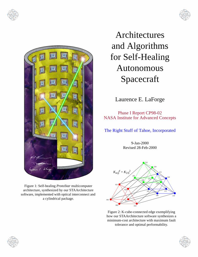
Figure 1: Self-healing ProtoStar multicomputerarchitecture, synthesized by our STAArchitecture
software, implemented with optical interconnect and a cylindrical package.
Figure 2: K-cube-connected edge exemplifying how our STAArchitecture software synthesizes a minimum-cost architecture with maximum fault
tolerance and optimal performability.
Km⋅jd = K2⋅3
2
000
001
020
021
010
011
100
101
110
111
120
121
200
201
220
221
210
211
Cover background from [Milky Way 1999]. Cover design by Derek Carlson.
Architectures and Algorithms for Self-Healing Autonomous Spacecraft
Table of Contents
1. Executive Summary ……………………………………………………………………………… 3
2. Starships Require Revolutionary Autonomy, Survivability, and Performance……………………… 4
3. Starchart Genesis: Enabling Characteristics of Starship Software and Avionics ………………… 7
3.1 Autonomous Intelligence: Roving Astronomers-on-a-Computer …………………………… 8
3.2 Avionics: The Best Supporting Actor for Self-Adapting Software ………………………… 8
3.3 Autonomous Intelligence: Demands for More Computing Power (More’s Law) …………… 8
3.4 Autonomous Intelligence: Experimentally Substantiated Workloads ……………………… 8
3.5 Autonomous Intelligence: From Science to Self-Healing Architectures and Algorithms …… 9
3.6 Self-Healing Architectures: Survivable in the Presence of a High Proportion of Faults …… 10
3.7 Self-Healing Algorithms: Autonomous Configuration of Healthy Quorums ……………… 12
3.8 Self-Healing Algorithms: Identification of Faults via Mutual Test and Diagnosis ………… 12
3.9 Self-Healing Architectures: Switching and Routing Governed Locally …………………… 13
3.10 Avionics: Switch Technologies Biased Against Stuck-Closed Faults ……………………… 13
3.11 Avionics: Interconnection Three-Space is Free Space ……………………………………… 13
3.12 Avionics: Shielding and Hardening to 104 Mrad(Si)………………………………………… 14
3.13 Avionics and Software: Reused Components Must Meet Requirements …………………… 15
3.14 Design Tools and Processes: Resistance is Futile – Embrace the Next Generation ………… 15
3.15 Design Tools and Processes: High Yield Enhances Reliability……………………………… 18
3.16 Design Tools and Processes: Measure Those Software Failures and Faults! ……………… 18
3.17 Design Processes: Programmatic Support Bolsters Breakthroughs ………………………… 20
4. Advances in Self-Healing Architectures and Algorithms ………………………………………… 21
4.1 Configuration: STAArchitecture Connects the Dots ………………………………………… 22
4.2 Performability: STAArchitecture Applies Knowledge About Distance……………………… 26
4.3 Performability: STAArchitecture Reflects New Results About Quorums from C-Cubes…… 35
4.4 Performability: High Fidelity Results for Quorum Radius and Diameter …………………… 43
4.5 Performability of Large Scale Architectures ……………………………………………… 48
4.6 Diagnosis and Configuration: STAArchitecture Simulates Distributed Algorithms ………… 51
5. Starchart For a ProtoStar Multicomputer ………………………………………………………… 54
Appendix A. References ……………………………………………………………………………… 55
The Right Stuff of Tahoe, Inc.The Right Place
3341 Adler CourtReno, NV 89503-1263
Phase I Report CP98-02NASA Institute for Advanced Concepts
Copyright © 2000
Laurence E. LaForge
Tel: (775) 322-5186Fax: (775) 322-5182
Self-Healing Autonomous Spacecraft Table of Contents
NASA Institute for Advanced Concepts 2 Phase I Report, Revision 30-Jan-2000
This revision reflects clarifications and corrections to versions issued 9, 12, and 30-Jan-2000.
Accompanying software. This report is accompanied by version 0.5 of STAArchitecture, a 32-bit Win-dows program described in Section 4. For operational and licensing information about STAArchitecture,refer to the readme.txt bundled with the online or CD ROM distribution kit. Also included in the distribu-tion kit: astronomical-proportions.xls, a Microsoft Excel 97 spreadsheet that contains many of the calcula-tions and charts featured herein. "STAArchitecture" and "Astronomical Proportions" are trademarks ofThe Right Stuff of Tahoe, Incorporated.a
Acknowledgments. At The Right Stuff of Tahoe, my co-investigators, Kirk F. Korver andDerek D. Carlson, wrote the STAArchitecture software, managed our office and accounts, performed liter-ature searches, checked out mathematical models, and assisted with the production of this report. MyronHecht of SoHAR elaborated ideas for self-healing software. Christopher R. Cassellb of Lockheed Martinlent his expert guidance in our calculations for Figure 5. Also of Lockheed Martin, Joe Marshall and DavidMeyer generously explained state-of-the-art radiation-hardened microcircuits, while Homayoun Malekprovided insight into differences and similarities between starship applications and the Theater High-Alti-tude Area Defense program (Thaad) [Lewis and Postol 1997], [Stein and Little 1997]. For the Hertzs-prung-Russell diagram of Figure 3, Roger A. Freedman of the University of California at Santa Barbaragraciously secured permission from W. H. Freeman and Company to reproduce Figure 19-13 of Universe[Kaufmann and Freedman 1999], the wonderful astronomy text he wrote with William J. Kaufmann III.
I am particularly indebted to Sarah A. Gavit for sharing the results of her team's work on the JPL Interstel-lar Probe. Her colleagues at NASA facilities – Ames Research Center, Glenn Research Center, the Jet Pro-pulsion Laboratory, Kennedy Space Center, Langley Research Center, Marshall Space Flight Center, andWashington Headquarters – provided additional valuable material, both written and spoken. Though gen-erally credited among the references of Appendix A, I would like to reiterate my appreciation to:Leon Alkalai, John R. Anderson, Robert C. Barry, Douglas E. Bernard, N. Talbot Brady, W. H. Bryant,Savio N. Chau, John Cole, James M. Dumoulin, Daniel L. Dvorak, David J Eisenman, Daniel B. Eldred,Daniel E. Erickson, Martin S. Feather, Dwight A. Geer, Peter R. Glück, Daniel S. Goldin,Cecilia N. Guiar, Keith D. Goodfellow, Donald J. Hunter, Sanford M. Krasner, Vincent R. Lalli,David H. Lehman, Michael R. Lowry, Marc G. Millis, David Morrison, Brian K. Muirhead,Allen P. Nikora, Peter Norvig, John C. Peterson, Robert D. Rasmussen, Allan L. Sacks, Joseph L. Savino,Francis L. Schneider, Greg Schmidt, Burton C. Sigal, Carl N. Steiner, Samuel L. Venneri, andDavid F. Woerner.
I would also like to express my appreciation to colleagues at Embry-Riddle Aeronautical University. In theCollege of Career Education: Dr. William Getter, Dean of Academics. At the Hunt Memorial Library: AnnCash, Ellen Dewkett, Kathleen Chumley, Maria O' Brien, and Christine Poucher.
Thank you, one and all!
a. The logo in the corners of these pages is also a trademark of The Right Stuff of Tahoe, Incorporated. It depicts thesecond smallest member of a class of graphs, discovered in the early 1990’s to be almost surely diagnosable at con-stant test redundancy [LaForge et al 1993].
b. Representing himself.
Self-Healing Autonomous Spacecraft 1. Executive Summary
NASA Institute for Advanced Concepts 3 Phase I Report, Revision 30-Jan-2000
1. Executive Summary
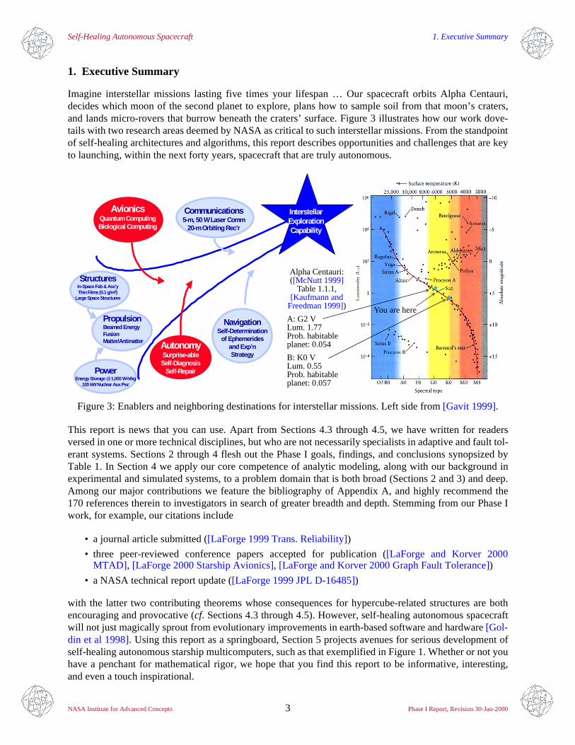
Imagine interstellar missions lasting five times your lifespan … Our spacecraft orbits Alpha Centauri,decides which moon of the second planet to explore, plans how to sample soil from that moon’s craters,and lands micro-rovers that burrow beneath the craters’ surface. Figure 3 illustrates how our work dove-tails with two research areas deemed by NASA as critical to such interstellar missions. From the standpointof self-healing architectures and algorithms, this report describes opportunities and challenges that are keyto launching, within the next forty years, spacecraft that are truly autonomous.
This report is news that you can use. Apart from Sections 4.3 through 4.5, we have written for readersversed in one or more technical disciplines, but who are not necessarily specialists in adaptive and fault tol-erant systems. Sections 2 through 4 flesh out the Phase I goals, findings, and conclusions synopsized byTable 1. In Section 4 we apply our core competence of analytic modeling, along with our background inexperimental and simulated systems, to a problem domain that is both broad (Sections 2 and 3) and deep.Among our major contributions we feature the bibliography of Appendix A, and highly recommend the170 references therein to investigators in search of greater breadth and depth. Stemming from our Phase Iwork, for example, our citations include
• a journal article submitted ([LaForge 1999 Trans. Reliability])
• three peer-reviewed conference papers accepted for publication ([LaForge and Korver 2000MTAD] , [LaForge 2000 Starship Avionics], [LaForge and Korver 2000 Graph Fault Tolerance])
• a NASA technical report update ([LaForge 1999 JPL D-16485])
with the latter two contributing theorems whose consequences for hypercube-related structures are bothencouraging and provocative (cf. Sections 4.3 through 4.5). However, self-healing autonomous spacecraftwill not just magically sprout from evolutionary improvements in earth-based software and hardware [Gol-din et al 1998]. Using this report as a springboard, Section 5 projects avenues for serious development ofself-healing autonomous starship multicomputers, such as that exemplified in Figure 1. Whether or not youhave a penchant for mathematical rigor, we hope that you find this report to be informative, interesting,and even a touch inspirational.
Figure 3: Enablers and neighboring destinations for interstellar missions. Left side from [Gavit 1999].
AvionicsQuantum ComputingBiological Computing
AutonomySurprise-ableSelf-Diagnosis
Self-Repair
Communications5-m, 50 W Laser Comm
20-m Orbiting Rec’r
InterstellarExplorationCapability
PropulsionBeamed EnergyFusionMatter/Antimatter
StructuresIn-Space Fab & Ass’yThin Films (0.1 g/m 2)
Large Space Structures
PowerEnergy Storage @ 1,000 W-h/kg
100 kW Nuclear Aux Pwr
NavigationSelf-Determination
of Ephemeridesand Exp’nStrategy
Alpha Centauri:([McNutt 1999]
Table 1.1.1, [Kaufmann and
Freedman 1999])
A: G2 VLum. 1.77Prob. habitable planet: 0.054
B: K0 VLum. 0.55Prob. habitable planet: 0.057
You are here
Self-Healing Autonomous Spacecraft 2. Starships Require Revolutionary Autonomy, Survivability, and Performance
NASA Institute for Advanced Concepts 4 Phase I Report, Revision 30-Jan-2000
2. Starships Require Revolutionary Autonomy, Survivability, and Performance
Perhaps more than any other factor, distance provides the impetus for spacecraft autonomy ([Goldsmith1999], Chap. 9). Our knowledge of a spacecraft’s environment diminishes with increasing distance fromearth (but this makes the mission more interesting). Distance dictates communication latency: to arrive at aprobe near Pluto,1 for example, a radio signal travels for more than five hours – entirely too long for earth-bound controllers to tactically adapt the spacecraft to changes in environment.
Distance also dominates properties of self-healing avionics and software. Most prominently, the time for aprobe to complete its mission is bounded from below by the length of the journey divided by the speed pro-vided by our best propulsion. For either hardware or software, the cumulative probability of failureincreases with the time of operation.2 Mission duration is therefore a major challenge for continuouslyavailable avionics and software. These observations underscore why revolutions in self-healing autonomyare most needed, and why they are most likely to be devised, for long distance missions of long duration.
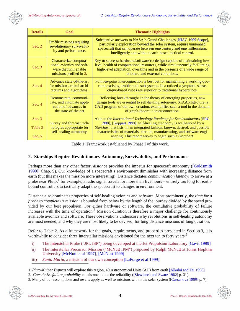
Refer to Table 2. As a framework for the goals, requirements, and properties presented in Section 3, it isworthwhile to consider three interstellar missions envisioned for the next ten to forty years:3
i) The Interstellar Probe ("JPL ISP") being developed at the Jet Propulsion Laboratory [Gavit 1999]ii) The Interstellar Precursor Mission ("McNutt IPM") proposed by Ralph McNutt at Johns Hopkins
University [McNutt et al 1997], [McNutt 1999]iii) Santa Maria, a mission of our own conception [LaForge et al 1999]
Details Goal Thematic Highlights
Sec. 2Profile missions requiring revolutionary survivabil-
ity and performance.
Substantive answers to NASA’s Grand Challenges [NIAC 1999 Scope], particularly exploration beyond the solar system, require unmanned
spacecraft that can operate between one century and one millennium, intelligently and without earth-based tactical control.
Sec. 3
Characterize computa-tional avionics and soft-
ware that will enable missions profiled in 2.
Key to success: hardware/software co-design capable of maintaining low-level health of computational resources, while simultaneously facilitating high-level adaptation, over time and in the presence of a wide range of
onboard and external conditions.
Sec. 4Advance state-of-the-art for mission-critical archi-tectures and algorithms.
Point-to-point interconnection is best bet for maintaining a working quo-rum, excising problematic subsystems. In a ratioed asymptotic sense,
clique-based cubes are superior to traditional hypercubes.
Sec. 4
Demonstrate, communi-cate, and automate appli-
cation of advances inthe state-of-the-art
Reflecting breakthroughs in the theory of emerging properties, new design tools are essential to self-healing autonomy. STAArchitecture, a
CAD program of our own creation, exemplifies such a tool in the domain of graph-theoretic interconnection.
Sec. 3
Table 3
Sec. 5
Survey and forecast tech-nologies appropriate for self-healing autonomy.
Akin to the International Technology Roadmap for Semiconductors [SRC 1998], [Geppert 1999], self-healing autonomy is well-served by a
Starchart that lists, in an integrated fashion, known, desired, and possible characteristics of materials, circuits, manufacturing, and software engi-
neering. This report serves to begin such a Starchart.
Table 1: Framework established by Phase I of this work.
1. Pluto-Kuiper Express will explore this region, 40 Astronomical Units (AU) from earth [Alkalai and Tai 1998].2. Cumulative failure probability equals one minus the reliability ([Siewiorek and Swarz 1982] p. 31).3. Many of our assumptions and results apply as well to missions within the solar system ([Cassanova 1999] p. 7).
Self-Healing Autonomous Spacecraft 2. Starships Require Revolutionary Autonomy, Survivability, and Performance
NASA Institute for Advanced Concepts 5 Phase I Report, Revision 30-Jan-2000
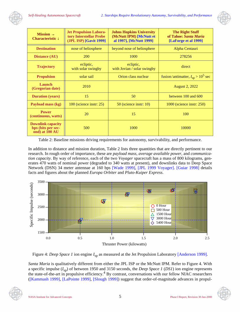
In addition to distance and mission duration, Table 2 lists three quantities that are directly pertinent to ourresearch. In rough order of importance, these are payload mass, average available power, and communica-tion capacity. By way of reference, each of the two Voyager spacecraft has a mass of 800 kilograms, gen-erates 470 watts of nominal power (degraded to 340 watts at present), and downlinks data to Deep SpaceNetwork (DSN) 34 meter antennae at 160 bps [Wade 1999], [JPL 1999 Voyager]. [Guiar 1998] detailsfacts and figures about the planned Europa Orbiter and Pluto-Kuiper Express.
Santa Maria is qualitatively different from either the JPL ISP or the McNutt IPM. Refer to Figure 4. Witha specific impulse (Isp) of between 1950 and 3150 seconds, the Deep Space 1 (DS1) ion engine representsthe state-of-the-art in propulsive efficiency.4 By contrast, conversations with our fellow NIAC researchers([Kammash 1999], [LaPointe 1999], [Slough 1999]) suggest that order-of-magnitude advances in propul-
Mission →→Characteristic ↓↓
Jet Propulsion Labora-tory Interstellar Probe (JPL ISP) [Gavit 1999]
Johns Hopkins University (McNutt IPM) [McNutt et
al 1997], [McNutt 1999]
The Right Stuffof Tahoe: Santa Maria[LaForge et al 1999]
Destination nose of heliosphere beyond nose of heliosphere Alpha Centauri
Distance (AU) 200 1000 278256
Trajectory ecliptic,with solar swingby
ecliptic, with Jovian / solar swingby direct
Propulsion solar sail Orion class nuclear fusion/antimatter, Isp > 105 sec
Launch(Gregorian date) 2010 August 2, 2022
Duration (years) 15 50 between 100 and 600
Payload mass (kg) 100 (science instr: 25) 50 (science instr: 10) 1000 (science instr: 250)
Power(continuous, watts) 20 15 100
Downlink capacity bps (bits per sec-ond) at 100 AU
500 1000 10000
Table 2: Baseline missions driving requirements for autonomy, survivability, and performance.
Figure 4: Deep Space 1 ion engine Isp as measured at the Jet Propulsion Laboratory [Anderson 1999].
2.52.01.51.00.50.0
Thruster Power (kilowatts)
3500
3000
2500
2000
1500
Spec
ific
Im
puls
e (s
econ
ds)
0 Hour 500 Hour 1500 Hour 3000 Hour 5400 Hour
Self-Healing Autonomous Spacecraft 2. Starships Require Revolutionary Autonomy, Survivability, and Performance
NASA Institute for Advanced Concepts 6 Phase I Report, Revision 30-Jan-2000
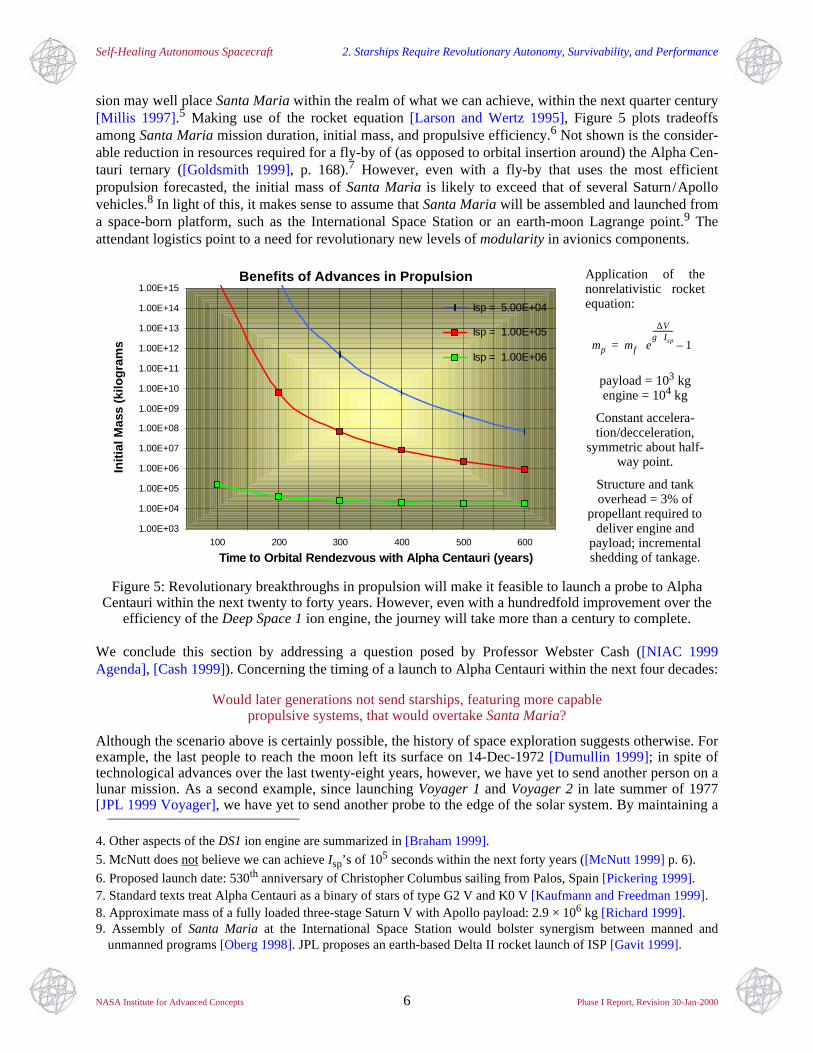
sion may well place Santa Maria within the realm of what we can achieve, within the next quarter century[Millis 1997].5 Making use of the rocket equation [Larson and Wertz 1995], Figure 5 plots tradeoffsamong Santa Maria mission duration, initial mass, and propulsive efficiency.6 Not shown is the consider-able reduction in resources required for a fly-by of (as opposed to orbital insertion around) the Alpha Cen-tauri ternary ([Goldsmith 1999], p. 168).7 However, even with a fly-by that uses the most efficientpropulsion forecasted, the initial mass of Santa Maria is likely to exceed that of several Saturn/Apollovehicles.8 In light of this, it makes sense to assume that Santa Maria will be assembled and launched froma space-born platform, such as the International Space Station or an earth-moon Lagrange point.9 Theattendant logistics point to a need for revolutionary new levels of modularity in avionics components.
We conclude this section by addressing a question posed by Professor Webster Cash ([NIAC 1999Agenda], [Cash 1999]). Concerning the timing of a launch to Alpha Centauri within the next four decades:
Would later generations not send starships, featuring more capablepropulsive systems, that would overtake Santa Maria?
Although the scenario above is certainly possible, the history of space exploration suggests otherwise. Forexample, the last people to reach the moon left its surface on 14-Dec-1972 [Dumullin 1999]; in spite oftechnological advances over the last twenty-eight years, however, we have yet to send another person on alunar mission. As a second example, since launching Voyager 1 and Voyager 2 in late summer of 1977[JPL 1999 Voyager], we have yet to send another probe to the edge of the solar system. By maintaining a
4. Other aspects of the DS1 ion engine are summarized in [Braham 1999].
5. McNutt does not believe we can achieve Isp’s of 105 seconds within the next forty years ([McNutt 1999] p. 6).
6. Proposed launch date: 530th anniversary of Christopher Columbus sailing from Palos, Spain [Pickering 1999].7. Standard texts treat Alpha Centauri as a binary of stars of type G2 V and K0 V [Kaufmann and Freedman 1999].8. Approximate mass of a fully loaded three-stage Saturn V with Apollo payload: 2.9 × 10⁶ kg [Richard 1999].9. Assembly of Santa Maria at the International Space Station would bolster synergism between manned and
unmanned programs [Oberg 1998]. JPL proposes an earth-based Delta II rocket launch of ISP [Gavit 1999].
Figure 5: Revolutionary breakthroughs in propulsion will make it feasible to launch a probe to Alpha Centauri within the next twenty to forty years. However, even with a hundredfold improvement over the
efficiency of the Deep Space 1 ion engine, the journey will take more than a century to complete.
Benefits of Advances in Propulsion
1.00E+03
1.00E+04
1.00E+05
1.00E+06
1.00E+07
1.00E+08
1.00E+09
1.00E+10
1.00E+11
1.00E+12
1.00E+13
1.00E+14
1.00E+15
100 200 300 400 500 600
Time to Orbital Rendezvous with Alpha Centauri (years)
Init
ial M
ass
(kilo
gra
ms)
Isp = 5.00E+04
Isp = 1.00E+05
Isp = 1.00E+06
Application of thenonrelativistic rocketequation:
payload = 103 kgengine = 104 kg
Constant accelera-tion/decceleration,
symmetric about half-way point.
Structure and tank overhead = 3% of
propellant required to deliver engine and
payload; incremental shedding of tankage.
mp mf e
∆Vg I⋅ sp
-------------
1–
=
3. Genesis of a Starchart for Software and Avionics Enabling Characteristics at a Glance
Self-Healing Autonomous Spacecraft 7 NIAC Phase I Report, Revision 28-Feb-2000
wait-and-see strategy for improvements in propulsion, moreover, we might never launch a mission toAlpha Centauri. Consistent with NIAC objectives [NIAC 1999 Scope], this report presumes, and further-more advocates, charting a course for Alpha Centauri at the earliest feasible opportunity. The remainingsections chart a course of feasible opportunities for self-healing computational avionics and software.
Goa
l/R
equi
rem
ent/
Pro
pert
y
Priorities for Success: Stars of the Main Sequence
Section 3 at a Glance
In-depth Research, Phase I:
STAArchitecture CAD Tool, Phase I:
Emphasis
Avi
onic
s
Aut
onom
ous
Inte
llige
nce
Sel
f-H
ealin
g A
rchs
. & A
lgs.
CA
D T
ools
Des
ign
Pro
cess
es
3.1 Payload: roving astronomer-on-a-computer.
3.2 Avionics targeted to support software that can learn and adapt on its own,occasionally guided via communication (albeit highly latent) with earth.
3.3 More’s Law:12 Autonomous Intelligence (AI) demands more computing power.
3.4Experimentally verified models quantify relations among processing power, low-
level tasks, and AI. 1015 ops/sec-kg provisional performance objective.
3.5 Four domains of knowledge and control: a) scientific; b) communication;c) navigation; d) self-healing starship control and maintenance.
3.6 Tolerance to a constant proportion of faulty computational nodes.
3.7 Self-configuring, uniform computational nodes maintain connectivityamong healthy nodes, disconnect healthy from faulty nodes.
3.8 Computational nodes identify faults via MTAD: mutual test and diagnosis.
3.9 Computational nodes govern their own switches for connecting to other nodes.
3.10 Switch technologies biased against stuck-closed faults.
3.11 Computational nodes connected by three-dimensional technology that mitigates, in order of priority: a) short circuits, b) mass, and c) signal delay.
3.12 Shielding and hardening to 104 Mrad(Si)
3.13 Reuse only components that match design requirements.
3.14 Teams embrace and exploit a new generation of CAD tools and processes.
3.15 Avionics and software designed for high yield as well as high reliability.
3.16 Instrument and measure software failures and faultsat quantifiable levels commensurate with physical measurements of avionics.
3.17 Administrators and managers actively promote, and participate in, development.
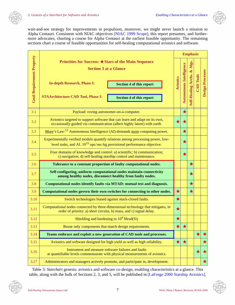
Table 3: Starchart genesis: avionics and software co-design, enabling characteristics at a glance. This table, along with the bulk of Sections 2, 3, and 5, will be published in [LaForge 2000 Starship Avionics].
Section 4 of this report
Section 4 of this report
3.1 – 3.5. Enabling Characteristics of Autonomous Intelligence Roving Astronomers-on-a-Computer
Self-Healing Autonomous Spacecraft 8 NIAC Phase I Report, Revision 28-Feb-2000
3. Starchart Genesis: Enabling Characteristics of Starship Software and Avionics
From the perspective of architectures and algorithms, Table 3 proffers priorities about what we shouldbuild and, furthermore, how we should go about building it. Though by no means exhaustive, characteris-tics 3.1 through 3.17 embrace the space of software/hardware co-design for self-healing autonomous star-ships. With respect to this design space, the descriptions, examples, and references cited in this sectionestablish a central role for self-healing architectures and algorithms (requirements 3.6 through 3.9,Section 4) as well as related tools (requirement3.14, Section 4) for computer aided design (CAD). Webegin with a position put forth by Dr. Daniel Dvorak and Dr. Richard Doyle at JPL [Dvorak and Doyle1998], and by Professor Sandra M. Faber of the University of California at Santa Cruz [Milky Way 1999]:
3.1 Starship payloads will be autonomous, intelligent, robots: roving astronomers-on-a-computer.10
As basic as 3.1 may be, it sets the stage for the computational tasks that avionics and software must per-form. While press reports may have exaggerated the success of the Deep Space 1 Remote Agent ([JPLDS1 Press Release], [Foust 1999]), real starship autonomy is within the twenty-year horizon of softwareengineering. JPL's X2000 Mission Data System is being built of Goal Achieving Modules (GAMS), anevolutionary successor to the Remote Agent [Dvorak 1998]. By any stretch of the imagination, therefore,starship avionics must provide the raw computational horsepower for successors to the Remote Agent.
Software is the only thing that we can add to a payload, once our starship has ventured into deep space;software provides a final degree of freedom in starship design and implementation. From this simpleobservation we see that a very real opportunity (and perhaps the best opportunity) for maximizing auton-omy is to ensure the starship software does not spend the time to destination spinning in an idle loop, butrather "grows up", in a fashion not unlike the way hominoids mature to adulthood:
3.2 Starship avionics will support software that can learn and adapt on its own,occasionally guided via communication (albeit highly latent) with earth.
As with other high-end applications, More's Law applies:
3.3 Autonomous intelligence (AI)11 will always demand more computing power,more memory, and more communications capacity.12
For any given level of AI, we can ask how much computing power will be needed to satisfyrequirements3.2 and 3.3. The open-ended nature of this requirement (what does it mean for software tolearn and adapt on its own?) renders such an assessment difficult. Refer to Figure 6. Our Phase I technicalproposal targeted a machine capable of retiring 1015 operations per second [LaForge 1999 NIAC Phase IProposal], and this appears to be achievable. Largely due to the dearth of models and experiments for char-acterizing AI workloads [Dvorak 1999], however, we really do not know if such performance is too little,too much, or about right. Section 5 identifies a number of tasks critical to workload characterization, at alevel of fidelity that will facilitate the design of self-healing architectures and algorithms. In the interim:
3.4 Successful design of self-healing autonomy will require experimentally verified models that quantify the relations among processing power, low-level tasks, and AI.13
1015 operations per second per kilogram is a provisional performance objective.
10. Even optimists doubt the feasibility of human interstellar exploration within the next forty years [Nordley 1998].11. AI = autonomous (not artificial) intelligence: intentional coining of new words for an old, artificial acronym.12. Requirement 3.3 articulates More’s Law. Moore's Law states that our capacity for packing circuit devices orinformation storage increases exponentially (alternatively, the price per circuit function or bit of storage decreasesexponentially), at between 2% and 4% per month [Schaller 1997], [Economist 1997], [Hamilton 1999].13. One possible application for experimentally quantifying such a workload: IVHM, an AI system for self-diagnosisof remote agents, spaceliners, and rotorcraft; under development at NASA Ames Research Center [Norvig 1999].
3.1 – 3.5. Enabling Characteristics of Autonomous Intelligence Roving Astronomers-on-a-Computer
Self-Healing Autonomous Spacecraft 9 NIAC Phase I Report, Revision 28-Feb-2000
Notwithstanding our inability to quantify the computational demands imposed by an autonomously intelli-gent workload, we can qualify some of the salient characteristics of such a system. For example, what kindof knowledge will our starship need to possess, and what kinds of things will it have to do in response to itsenvironment? Broadly speaking:
3.5 The combination of knowledge and control of actions (based on knowledge and input) can be divided into four domains: a) scientific; b) communication; c) navigation;14 d) starship control and mainte-nance, with the latter including self-healing architectures and algorithms for computational resources.
From a strategic perspective, science is the raison d’être for a starship: the navigation, communication, andinstrument control serve as means for conducting and reporting the outcome of science experiments. Froma tactical point of view, the order of priority is reversed: the starship’s computational health is necessary tosuccessfully determine location, trajectory, and control; accurate navigation is necessary to positioningspacecraft to carry out science experiments; the value of these experiments hinges on the starship’s abilityto communicate their outcomes to us. While our Phase I effort focuses on 3.5d, a comprehensive design ofhardware and software will take full account of 3.5a, b, and c. These domains are traditionally addressedby formulating specifications for onboard instrumentation. Refer to Table 4. While both the JPL ISP andthe McNutt IPM feature manifests for onboard scientific instruments ([Gavit 1999], [McNutt 1999]), nei-ther of these missions appears to have developed an analogous list for navigation and communication.15
The genesis of starship instrumentation may well result from a combination of evolution and revolution.For example, new discoveries of planets outside the solar system,16 perhaps with the aid of x-ray interfer-ometers like that proposed by Professor Webster Cash [Cash 1999 X-File], could shift our investigativepriorities to questions about astrobiology [Morrison and Schmidt 1999]. In the case of Santa Maria, it isbeyond our Phase I scope to draft a list of instruments – scientific, navigational, communication, or other-wise. However, Section 5 identifies collaborative tasks for composing, at an operational level of fidelity, amanifest for the Santa Maria payload. We anticipate a diverse yet coordinated suite of instruments, reflect-ing contributions from specialists in academia, industry, and government.
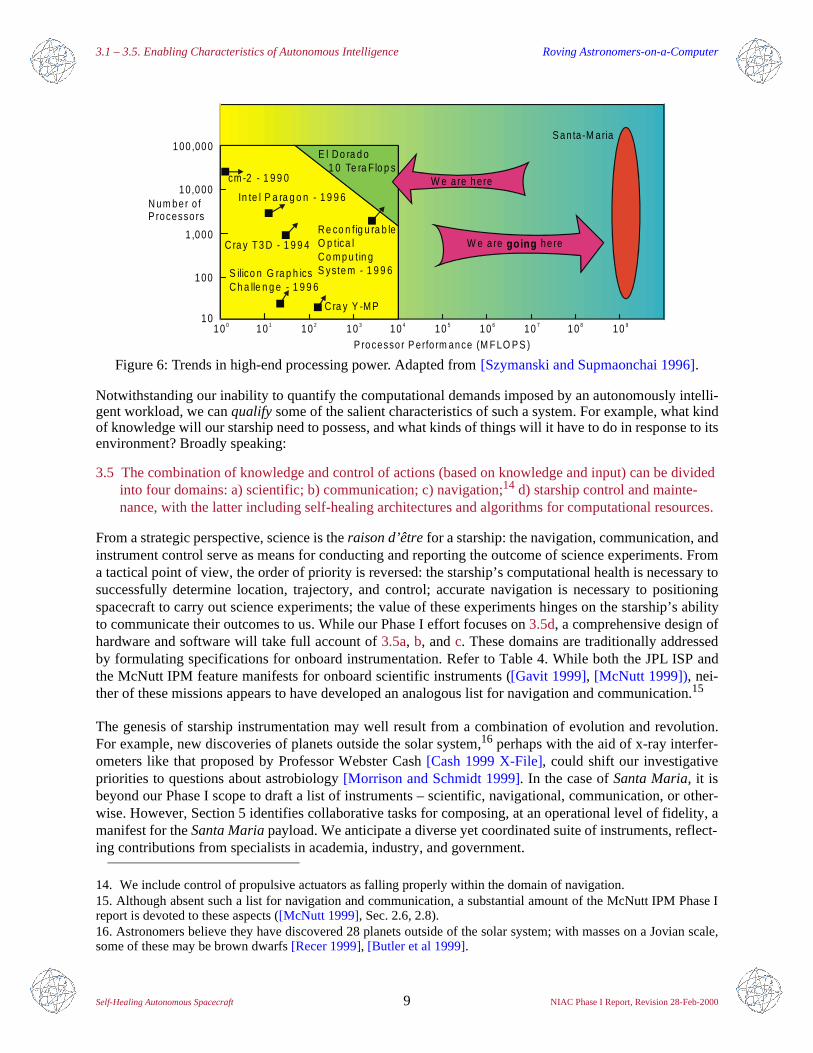
Figure 6: Trends in high-end processing power. Adapted from [Szymanski and Supmaonchai 1996].
14. We include control of propulsive actuators as falling properly within the domain of navigation.15. Although absent such a list for navigation and communication, a substantial amount of the McNutt IPM Phase Ireport is devoted to these aspects ([McNutt 1999], Sec. 2.6, 2.8).16. Astronomers believe they have discovered 28 planets outside of the solar system; with masses on a Jovian scale,some of these may be brown dwarfs [Recer 1999], [Butler et al 1999].
cm -2 - 1 9 9 0
In te l P a ra g o n - 1 9 9 6
C ra y T3 D - 1 9 9 4
S ilico n G ra p h icsC h a lle n g e - 1 9 9 6
C ra y Y -M P
E l D o ra d o1 0 Te ra F lo p s
iR e co n fig u ra b leO p t ca lC o m p u tin gS yste m - 1 9 9 6
100 ,000
10,000
1 ,000
100
1010 0 10 1 10 910 810 710 610 510 410 310 2
N um ber o fP rocesso rs
P rocesso r P erfo rm ance (M F LO P S )
W e a re here
W e a re he regoing
S an ta-M aria
Enabling Characteristics of Self-Healing Architectures 3.6. Tolerance to a Constant Proportion of Faults
Self-Healing Autonomous Spacecraft 10 NIAC Phase I Report, Revision 28-Feb-2000
Despite gaps in our understanding of the implications of the more strategic domains of 3.5, we can charac-terize many facets of computational avionics and software for interstellar missions. In particular, hardwaredependability is at least as important as computational power, and in this respect we can bracket both whatis required and what is possible. Contemporary spacecraft avionics are specified to tolerate one fault, per-haps two, and this limited tolerance is mandated without regard to either the component failure probabilityor the number of components [Barry 1998], [Guiar 1998]. On the other hand, estimates for the mean timeto failure (MTTF) of discrete components range from 100 to 1000 years [Avizienis 1999], [Virgras], [Har-ris]. In light of this, and taking into account burgeoning levels of system complexity:
3.6 Self-healing autonomous starships will tolerate a constant proportion of faulty computational nodes.17
Reflecting the needs generated by century-long interstellar missions, Professor Algirdas Avizienis of theUniversity of California at Los Angeles has outlined both the past and the future of fault tolerant computa-tional avionics [Avizienis 1999]. As to the latter, starships face three categories of threats: i) latent designfaults that remain onboard; ii) components wearing out; iii) transient faults, single or burst. To this list wewould like to add iv) permanent faults that arise during the mission, regardless of source (e.g., radiation,thermal cycling, metal migration, latchup)18.
JPL ISP Science instrument McNutt IPM
Yes Magnetometer 3.0 kg 0.5 watts
Yes Plasma wave / radio detector1.5 kg 2.5 watts
Yes Dust sensor
Yes Detector for cosmic rays, hydrogen, helium, electrons and positrons
1.0 kg 1.5 wattsYes Galactic cosmic ray composition analyzer
Yes Solar wind / interstellar plasma / electron sensor
Yes Pickup and interstellar ion composition analyzer
Yes Interstellar neutrals detector
2.0 kg 2.0 wattsYes Suprathermal ion / electron sensor
Yes Energetic neutral atom imager
Yes Infrared imager 1.5 kg 1.5 watts
Yes Ultraviolet photometer No
No Lyman-α imager 1.0 kg 2.0 watts
25 kg 20 watts All Science Instruments 10 kg 10 watts
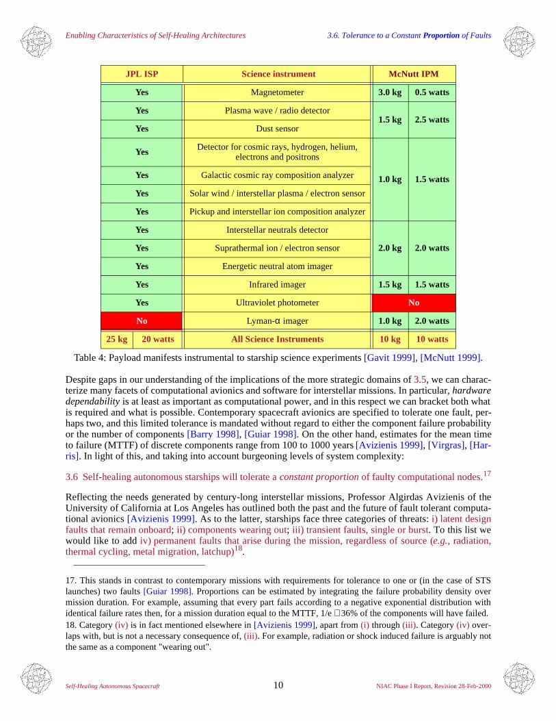
Table 4: Payload manifests instrumental to starship science experiments [Gavit 1999], [McNutt 1999].
17. This stands in contrast to contemporary missions with requirements for tolerance to one or (in the case of STSlaunches) two faults [Guiar 1998]. Proportions can be estimated by integrating the failure probability density overmission duration. For example, assuming that every part fails according to a negative exponential distribution withidentical failure rates then, for a mission duration equal to the MTTF, 1/e ≅ 36% of the components will have failed.18. Category (iv) is in fact mentioned elsewhere in [Avizienis 1999], apart from (i) through (iii) . Category (iv) over-laps with, but is not a necessary consequence of, (iii) . For example, radiation or shock induced failure is arguably notthe same as a component "wearing out".
Enabling Characteristics of Self-Healing Architectures 3.6. Tolerance to a Constant Proportion of Faults
Self-Healing Autonomous Spacecraft 11 NIAC Phase I Report, Revision 28-Feb-2000
The immune system paradigm proposed by [Avizienis 1999], and independently set forth by SoHaR Presi-dent Myron Hecht [LaForge et al 1999], appears to be a promising approach for addressing threats (i)through (iv). With all respect, however, the DiSTARS implementation advocated by Avizienis is not themost prudent use of redundancy. In particular, static, hardware-level distinction of computational nodes (asmaster, controlling, or defensive) is contrary to much of what we have learned in the three decades sincethe JPL STAR computer was designed [Avizienis 1967], [Hecht and Fiorentino 1988].
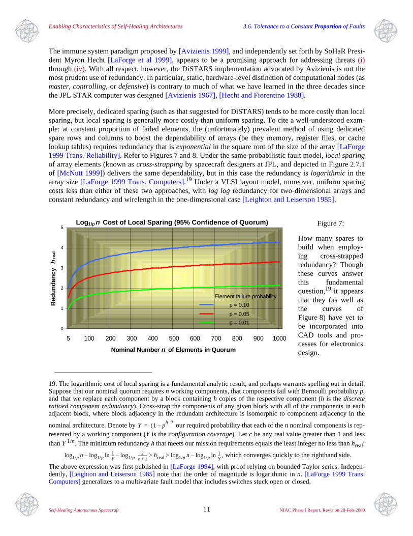
More precisely, dedicated sparing (such as that suggested for DiSTARS) tends to be more costly than localsparing, but local sparing is generally more costly than uniform sparing. To cite a well-understood exam-ple: at constant proportion of failed elements, the (unfortunately) prevalent method of using dedicatedspare rows and columns to boost the dependability of arrays (be they memory, register files, or cachelookup tables) requires redundancy that is exponential in the square root of the size of the array [LaForge1999 Trans. Reliability]. Refer to Figures 7 and 8. Under the same probabilistic fault model, local sparingof array elements (known as cross-strapping by spacecraft designers at JPL, and depicted in Figure 2.7.1of [McNutt 1999]) delivers the same dependability, but in this case the redundancy is logarithmic in thearray size [LaForge 1999 Trans. Computers].19 Under a VLSI layout model, moreover, uniform sparingcosts less than either of these two approaches, with log log redundancy for two-dimensional arrays andconstant redundancy and wirelength in the one-dimensional case [Leighton and Leiserson 1985].
19. The logarithmic cost of local sparing is a fundamental analytic result, and perhaps warrants spelling out in detail.Suppose that our nominal quorum requires n working components, that components fail with Bernoulli probability p,and that we replace each component by a block containing h copies of the respective component (h is the discreteratioed component redundancy). Cross-strap the components of any given block with all of the components in eachadjacent block, where block adjacency in the redundant architecture is isomorphic to component adjacency in the
nominal architecture. Denote by our required probability that each of the n nominal components is rep-resented by a working component (Y is the configuration coverage). Let c be any real value greater than 1 and lessthan Y 1 /n. The minimum redundancy h that meets our mission requirements equals the least integer no less than hreal:
, which converges quickly to the righthand side.
The above expression was first published in [LaForge 1994], with proof relying on bounded Taylor series. Indepen-dently, [Leighton and Leiserson 1985] note that the order of magnitude is logarithmic in n. [LaForge 1999 Trans.Computers] generalizes to a multivariate fault model that includes switches stuck open or closed.
Y 1 ph
–( )n
=
log1/p n log1/p ln 1Y---– log1/p 2
c 1+------------– hreal log1/p n log1/p ln 1
Y---–> >
Figure 7:
How many spares tobuild when employ-ing cross-strappedredundancy? Thoughthese curves answerthis fundamentalquestion,19 it appearsthat they (as well asthe curves ofFigure 8) have yet tobe incorporated intoCAD tools and pro-cesses for electronicsdesign.
Log1/p n Cost of Local Sparing (95% Confidence of Quorum)
0
1
2
3
4
5
5 100 200 300 400 500 600 700 800 900 1000
Nominal Number n of Elements in Quorum
Red
un
dan
cy
hre
al
Element failure probability
p = 0.10
p = 0.05
p = 0.01
3.7, 3.8. Enabling Characteristics of Architectures and Algorithms Self-Diagnosing, Self-Configuring Quorums
Self-Healing Autonomous Spacecraft 12 NIAC Phase I Report, Revision 28-Feb-2000
More generally, by relaxing constraints on the shape of our target architecture (e.g., not insisting on anarray), while at the same time maintaining uniformity among computational nodes, we can achieve highlysurvivable systems whose redundancy is (a best possible) constant. For illustration refer toFigures 1 and 2. Reflecting this, and by contrast to recent FAT-tree experiments with the Teramac super-computer [Clark 1998], [Culbertson et al 1997], [Culbertson et al 1996], Section 5 outlines tasks for creat-ing a family of optimally redundant starship multi-computer whose design devolves from a simplerequirement:
3.7 Computational starship avionics will consist of self-configuring, uniform computational nodes thatmaintain connectivity among healthy nodes, and that disconnect healthy from faulty nodes.
Such a collection of healthy nodes constitutes a quorum.20 Since cooperative computation requires thathealthy nodes communicate (and furthermore that they restrict communication with faulty nodes), 3.7 is afundamental criterion for self-healing autonomy. We may (and generally will) augment 3.7 with perfor-mance requirements for minimizing latency or maximizing throughput. Resurgent interest in combiningdependability with computational speed has sparked a relatively new area of research: performability[Haverkort and Niemegeers 1996]. Section 4 explains our Phase I contributions to performability theory,with novel emphasis on structure instead of traditional Markov chains [Nabli and Sericola 1996].
Consistent with requirements set forth by [Avizienis 1999]:
3.8 Computational nodes aboard starships will identify faults via MTAD: mutual test and diagnosis.
The need for distributed MTAD algorithms follows by observing that every node is subject to failure.Figure 9 depicts the relation between 3.7 and 3.8. As is the case with requirement 3.7, MTAD is essentialto self-healing autonomy [LaForge and Korver 2000 MTAD]. However, MTAD represents a radical depar-ture from traditional, centralized spacecraft fault protection ([Chau 1998 PDR], [LaForge 1999 JPL D-16485] pp. 58-70), and considerable experimental work remains to be done in order to best implementMTAD. In [LaForge and Korver 2000 MTAD] we describe how to go about performing these experiments.
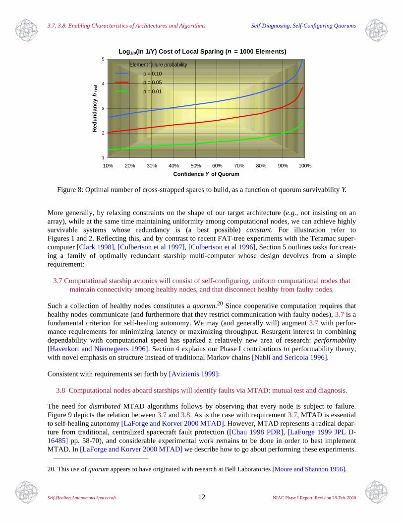
Figure 8: Optimal number of cross-strapped spares to build, as a function of quorum survivability Y.
20. This use of quorum appears to have originated with research at Bell Laboratories [Moore and Shannon 1956].
Log1/p(ln 1/Y) Cost of Local Sparing (n = 1000 Elements)
1
2
3
4
5
10% 20% 30% 40% 50% 60% 70% 80% 90% 100%
Confidence Y of Quorum
Red
un
dan
cy h
real
Element failure probability
p = 0.10
p = 0.05
p = 0.01
3.9 – 3.11. Enabling Characteristics of Switches and Interconnect Localized Control: Three-Space is Free Space
Self-Healing Autonomous Spacecraft 13 NIAC Phase I Report, Revision 28-Feb-2000
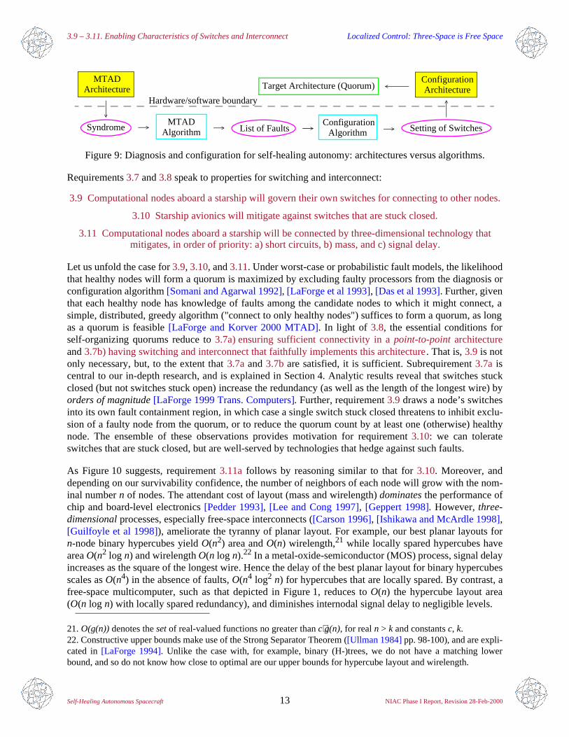
Requirements 3.7 and 3.8 speak to properties for switching and interconnect:
3.9 Computational nodes aboard a starship will govern their own switches for connecting to other nodes.
3.10 Starship avionics will mitigate against switches that are stuck closed.
3.11 Computational nodes aboard a starship will be connected by three-dimensional technology thatmitigates, in order of priority: a) short circuits, b) mass, and c) signal delay.
Let us unfold the case for 3.9, 3.10, and 3.11. Under worst-case or probabilistic fault models, the likelihoodthat healthy nodes will form a quorum is maximized by excluding faulty processors from the diagnosis orconfiguration algorithm [Somani and Agarwal 1992], [LaForge et al 1993], [Das et al 1993]. Further, giventhat each healthy node has knowledge of faults among the candidate nodes to which it might connect, asimple, distributed, greedy algorithm ("connect to only healthy nodes") suffices to form a quorum, as longas a quorum is feasible [LaForge and Korver 2000 MTAD]. In light of 3.8, the essential conditions forself-organizing quorums reduce to 3.7a) ensuring sufficient connectivity in a point-to-point architectureand 3.7b) having switching and interconnect that faithfully implements this architecture. That is, 3.9 is notonly necessary, but, to the extent that 3.7a and 3.7b are satisfied, it is sufficient. Subrequirement 3.7a iscentral to our in-depth research, and is explained in Section 4. Analytic results reveal that switches stuckclosed (but not switches stuck open) increase the redundancy (as well as the length of the longest wire) byorders of magnitude [LaForge 1999 Trans. Computers]. Further, requirement 3.9 draws a node’s switchesinto its own fault containment region, in which case a single switch stuck closed threatens to inhibit exclu-sion of a faulty node from the quorum, or to reduce the quorum count by at least one (otherwise) healthynode. The ensemble of these observations provides motivation for requirement 3.10: we can tolerateswitches that are stuck closed, but are well-served by technologies that hedge against such faults.
As Figure 10 suggests, requirement 3.11a follows by reasoning similar to that for 3.10. Moreover, anddepending on our survivability confidence, the number of neighbors of each node will grow with the nom-inal number n of nodes. The attendant cost of layout (mass and wirelength) dominates the performance ofchip and board-level electronics [Pedder 1993], [Lee and Cong 1997], [Geppert 1998]. However, three-dimensional processes, especially free-space interconnects ([Carson 1996], [Ishikawa and McArdle 1998],[Guilfoyle et al 1998]), ameliorate the tyranny of planar layout. For example, our best planar layouts forn-node binary hypercubes yield O(n2) area and O(n) wirelength,21 while locally spared hypercubes havearea O(n2 log n) and wirelength O(n log n).22 In a metal-oxide-semiconductor (MOS) process, signal delayincreases as the square of the longest wire. Hence the delay of the best planar layout for binary hypercubesscales as O(n4) in the absence of faults, O(n4 log2 n) for hypercubes that are locally spared. By contrast, afree-space multicomputer, such as that depicted in Figure 1, reduces to O(n) the hypercube layout area(O(n log n) with locally spared redundancy), and diminishes internodal signal delay to negligible levels.
Figure 9: Diagnosis and configuration for self-healing autonomy: architectures versus algorithms.
21. O(g(n)) denotes the set of real-valued functions no greater than c⋅g(n), for real n > k and constants c, k.22. Constructive upper bounds make use of the Strong Separator Theorem ([Ullman 1984] pp. 98-100), and are expli-cated in [LaForge 1994]. Unlike the case with, for example, binary (H-)trees, we do not have a matching lowerbound, and so do not know how close to optimal are our upper bounds for hypercube layout and wirelength.
Setting of Switches
Hardware/software boundary
MTAD
Setting of SwitchesList of Faults
Target Architecture (Quorum)Architecture
ConfigurationAlgorithm
ConfigurationArchitecture
MTADAlgorithmSyndrome
3.12. Radiation Resistant Avionics Shielding and Hardening to 104 Mrad(Si)
Self-Healing Autonomous Spacecraft 14 NIAC Phase I Report, Revision 28-Feb-2000
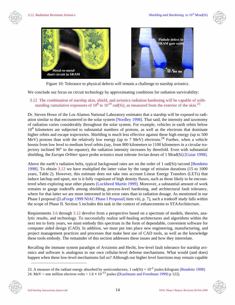
We conclude our focus on circuit technology by approximating conditions for radiation survivability:
3.12 The combination of starship skin, shield, and avionics radiation hardening will be capable of with-standing cumulative exposures of 108 to 1010 rad(Si), as measured from the exterior of the skin.23
Dr. Steven Howe of the Los Alamos National Laboratory estimates that a starship will be exposed to radi-ation similar to that encountered in the solar system [Nordley 1998]. That said, the intensity and taxonomyof radiation varies considerably throughout the solar system. For example, vehicles in earth orbits below104 kilometers are subjected to substantial numbers of protons, as well as the electrons that dominatehigher orbits and escape trajectories. Shielding is much less effective against these high energy (up to 500MeV) protons than with the relatively low energy (up to 7 MeV) electrons.24 Further, when a vehicleboosts from low level to medium level orbits (say, from 800 kilometers to 1100 kilometers in a circular tra-jectory inclined 90° to the equator), the radiation intensity increases by threefold. Even with substantialshielding, the Europa Orbiter space probe avionics must tolerate Jovian doses of 1 Mrad(Si) [Guiar 1998].
Above the earth’s radiation belts, typical background rates are on the order of 1 rad(Si)/second [Bendetto1998]. To obtain 3.12 we have multiplied the latter value by the range of mission durations (15 to 1000years, Table 2). However, this estimate does not take into account Linear Energy Transfers (LETs) thatinduce latchup and upset, nor is it fully cognizant of high density fluxes, such as those likely to be encoun-tered when exploring near other planets [Lockheed Martin 1999]. Moreover, a substantial amount of workremains to gauge tradeoffs among shielding, process-level hardening, and architectural fault tolerance,where for that latter we are more interested in bit error rates than in radiation dosage. As mentioned in ourPhase I proposal ([LaForge 1999 NIAC Phase I Proposal] item viii, p. 7), such a tradeoff study falls withinthe scope of Phase II. Section 5 includes this task in the context of enhancements to STAArchitecture.
Requirements 3.6 through 3.12 devolve from a perspective based on a spectrum of models, theories, ana-lytic results, and technology. To successfully realize self-healing architectures and algorithms within thenext ten to forty years, we must embody this spectrum in the form of dependable, convenient software forcomputer aided design (CAD). In addition, we must put into place new engineering, manufacturing, andproject management practices and processes that make best use of CAD tools, as well as the knowledgethese tools embody. The remainder of this section addresses these issues and how they interrelate.
Recalling the immune system paradigm of Avizienis and Hecht, low-level fault tolerance for starship avi-onics and software is analogous to our own cellular-level defense mechanisms. What would (and does)happen when these low-level mechanisms fail us? Although our higher level functions may remain capable
Figure 10: Tolerance to physical defects will remain a challenge to starship avionics.
23. A measure of the radiant energy absorbed by semiconductors, 1 rad(Si) = 10-2 joules/kilogram [Bendetto 1998].24. MeV = one million electron volts = 1.6 × 10⁻¹³ joules ([Kaufmann and Freedman 1999] p 122).
Metal-to-metalshort circuit in SRAM
Pinhole defect inDRAM gate oxide
Enabling Characteristics of Starship Software and Avionics 3.13. Reused Components Must Meet Requirements
Self-Healing Autonomous Spacecraft 15 NIAC Phase I Report, Revision 28-Feb-2000
of defending us against macro-level threats (such as rush-hour drivers), we run the risk of succumbing to acommon cold. Under conditions other than those for which they were originally designed, electronics andsoftware components rarely exhibit effective defenses [Zorian et al 1999], [Lowry 1998]. Unbridled reuseof such components risks our system succumbing to the bit-level analogy of a common cold. This pertainsin particular to commercial, off-the-shelf components (COTS):
3.13 Unbridled reuse of software or hardware components, with or without wrappers,impedes self-healing starship autonomy. This applies to COTS in particular.
[Avizienis 1997] articulates the case for considered, conservative application of COTS, a position ampli-fied by York University Professor John McDermid [McDermid and Talbert 1998]:
… It would worry me if people in aerospace and nuclear power industries started using a COTSsolution without a clear demonstration that it fits all requirements … A major drawback to wrappers… is that you may need to make them extremely complex to interact with the COTS component.
On the other hand, a component need not be of strictly commercial origin in order to be reused –or misused. Perhaps the most dramatic misuse of previously constructed components is the explosive fail-ure of Ariane 5. The fault that led to this failure was a consequence of plugging Ariane 4 flight softwareinto successor spacecraft, without taking full account of the behavior of the reused component viz. varia-tions in launch sequence [Aviation Week 1997], [Jezequel and Meyer 1997]. Moreover, such malpracticeis not the exclusive province of the European Space Agency. We underscore this point with two of our ownNASA spacecraft design experiences – one software, one hardware.
Deep Space 1 inherited much of its software from Mars Pathfinder. Unlike Pathfinder, however, DS1 car-ried no planetary rover. Recognizing the Ariane lesson, the DS1 flight software team attempted to excisePathfinder code pertaining to the Sojourner rover. However, removing the code rendered the DS1 flightsoftware incapable of being compiled and linked. DS1 and Pathfinder team members expended at leastthree calendar weeks rectifying this problem. During that time, concurrent development on flight softwarewas substantially impeded [Eldred 1997], [Dornheim 1998]. This example exemplifies the cost of reuse:usually hidden, frequently exorbitant.
As to hardware, the original X2000 design prescribed 1394 Firewire Bus controllers based on COTS intel-lectual property ("IP", expressed in Verilog or VHDL design languages). Firewire is not designed to toler-ate faulty nodes, and the boot sequence forbids cycles in the point-to-point connectivity. Projectrequirements necessitated redundant wiring paths [Guiar 1998], thus introducing cycles. In consequence,the 1394 IP was subjected to conditions other than those for which it was originally designed. Properaccommodation of these conditions warranted modifying and testing the IP hardware. Instead, these modi-fications were relegated to software. Although feasible to some extent, this approach exposed the avionicsto a number of debilitating low-level hardware faults [LaForge 1999 JPL D-16485].25 This example illus-trates a common reluctance to "pry open the black box"; when such reluctance prevails, "ticking box" ismore apt. How we come to so readily accept such ticking boxes brings to light to a broader issue:
3.14 Starship design teams must embrace a new generation of CAD tools and attendant processes.
Reflecting on our examples with DiSTARS and X2000 Firewire, we should expect sub-optimal,shoot-from-the-hip avionics and software whenever engineers are forced to produce designs outside oftheir respective specialties. To some extent this a downside of contemporary emphasis on cheaper space-craft [Woerner and Lehman 1995], [Broad 1999]. However, the point of the examples extends to all areas
25. Among other advances initially planned, 1394 Firewire was eventually descoped from X2000 [Chau 1999].37
Computer Aided Design: Tools and Processes 3.14. Resistance is Futile – Embrace the Next Generation
Self-Healing Autonomous Spacecraft 16 NIAC Phase I Report, Revision 28-Feb-2000
of software/hardware co-design. The cost of applying expert knowledge can be managed, and evenreduced, by employing processes that make judicious use of Computer Aided Design (CAD) [Bryant et al1989]. Epitomizing this approach, the semiconductor industry has very effectively ameliorated the need forlarge numbers of specialists by using CAD tools that, conveniently and dependably, incorporate the rigorand knowledge of experts. In the domain of spacecraft avionics and software, the outlook for requirement3.14 appears promising. Spearheading research in the integration of CAD tools and processes, for example,NASA’s Langley Research Center has partnered with the University of Virginia in creating the IntelligentSynthesis Environment (ISE) [Goldin et al 1998]. At the Jet Propulsion Laboratory, Mike Dickerson headsthe recently-formed Design Center, whose charter mirrors that of ISE [Chau 1999].
The promising outlook for 3.14 is bolstered by emerging levels of accessibility and capability for individ-ual CAD tools. For example, automated theorem proving can be used to rigorously establish the correct-ness of software. Once thought to be an academic exercise, this technique is now a practical reality[Neumann 1996]. By way of illustration, the Automated Software Engineering group at NASA’s AmesResearch Center has created Amphion, a tool that mechanizes system-level verification in the face ofevolving changes in application software; Amphion has been applied to problems in fluid dynamics andspace shuttle navigation [Lowry 1998], and was used to find flaws in the DS1 Remote Agent not uncov-ered through testing [Feather 1999]. At the Jet Propulsion Laboratory, researchers have repaired Cassiniflight software by employing SPIN, a verification tool akin to Amphion [Schneider 1999 E1].26
Recent advances in architectural CAD tools combine computer software with classical hardware domains,such as power engineering. At Penn State University, for example, Mary Jane Irwin and VijaykrishnanNarayanan have developed a tool that enables the designer to predict electrical power consumption basedon software instruction mix [Irwin and Narayanan 1999]. At the level of system reliability, designers arenow able to conveniently manipulate graphical interfaces that detail the dynamics of architectures sub-jected to faults. This capability is demonstrated by tools such as Relex®, developed by Relex SoftwareCorporation [Relex 1998], and MEADEP, developed by SoHaR [Tang et al 1998]. With respect to archi-tectural requirements 3.6, 3.7, and 3.8, our own STAArchitecture program allows the user to synthesizeand analyze computational avionics. As described in Section 4, STAArchitecture maximizes the probabil-ity of diagnosing and configuring a healthy quorum, while simultaneously minimizing cost and latency.27
To be sure, there remain gaps between what CAD tools are capable of doing and what they should do.Dependability analyzers, such as Relex® and MEADEP, tend to be very good at revealing behavior of agiven design ("what is the probability of 100 nodes surviving and computing together for 50 years?"), butfall short when it comes to computing optimal allocations of resources, such as redundancy ("what is theminimally redundant way of connecting nodes so that at least 100 survive and compute together for 50years?") Refer to Figures 7 and 8. Even the simplest techniques for organizing redundancy, such as localsparing, seem to be have been overlooked. Tools such as STAArchitecture serve to bridge these gaps.
Much more serious than gaps in CAD tool functionality: organizations frequently starve the adoption ofnew tools and processes, through either shear inertia or by active resistance. Economies of scale mayaccount for some starvation: by comparison with semiconductor products, spacecraft design is a relativelysmall niche. Nevertheless, we would be remiss to understate the importance and difficulty of integratingbreakthrough CAD tools and processes into spacecraft development teams. Figure 11 illustrates this wide-spread problem, one which severely impedes the advent of self-healing avionics and software.
26. Amphion is based on process algebra; SPIN uses model checking [Schneider 1999 E2].27. Cf. Figures 15 through 20. It is beyond our scope to attempt a comprehensive survey of CAD tools forsoftware/hardware co-design; such a task is being undertaken by JPL’s Design Center [Chau 1999]. Rather, ourobjective is to indicate the importance and benefits of architectural-level CAD to self-healing autonomous starships.
Computer Aided Design: Tools and Processes 3.14. Resistance is Futile – Embrace the Next Generation
Self-Healing Autonomous Spacecraft 17 NIAC Phase I Report, Revision 28-Feb-2000
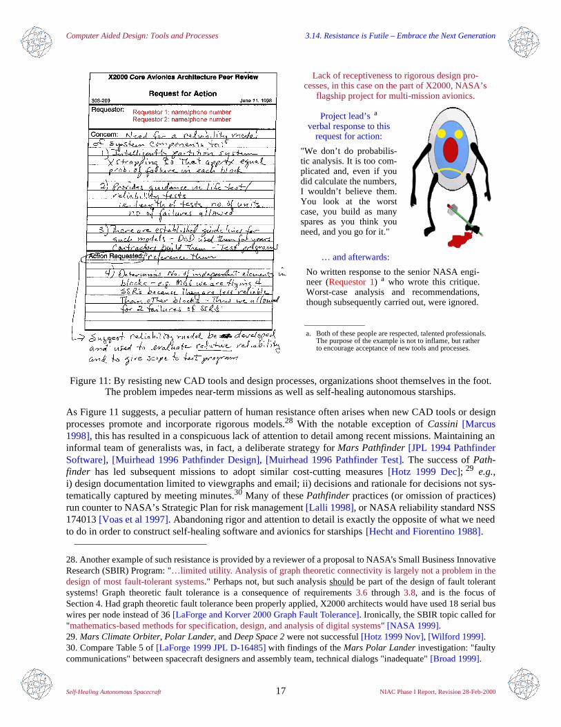
As Figure 11 suggests, a peculiar pattern of human resistance often arises when new CAD tools or designprocesses promote and incorporate rigorous models.28 With the notable exception of Cassini [Marcus1998], this has resulted in a conspicuous lack of attention to detail among recent missions. Maintaining aninformal team of generalists was, in fact, a deliberate strategy for Mars Pathfinder [JPL 1994 PathfinderSoftware], [Muirhead 1996 Pathfinder Design], [Muirhead 1996 Pathfinder Test]. The success of Path-finder has led subsequent missions to adopt similar cost-cutting measures [Hotz 1999 Dec]; 29 e.g.,i) design documentation limited to viewgraphs and email; ii) decisions and rationale for decisions not sys-tematically captured by meeting minutes.30 Many of these Pathfinder practices (or omission of practices)run counter to NASA’s Strategic Plan for risk management [Lalli 1998], or NASA reliability standard NSS174013 [Voas et al 1997]. Abandoning rigor and attention to detail is exactly the opposite of what we needto do in order to construct self-healing software and avionics for starships [Hecht and Fiorentino 1988].
Figure 11: By resisting new CAD tools and design processes, organizations shoot themselves in the foot. The problem impedes near-term missions as well as self-healing autonomous starships.
28. Another example of such resistance is provided by a reviewer of a proposal to NASA’s Small Business InnovativeResearch (SBIR) Program: "…limited utility. Analysis of graph theoretic connectivity is largely not a problem in thedesign of most fault-tolerant systems." Perhaps not, but such analysis should be part of the design of fault tolerantsystems! Graph theoretic fault tolerance is a consequence of requirements 3.6 through 3.8, and is the focus ofSection 4. Had graph theoretic fault tolerance been properly applied, X2000 architects would have used 18 serial buswires per node instead of 36 [LaForge and Korver 2000 Graph Fault Tolerance]. Ironically, the SBIR topic called for"mathematics-based methods for specification, design, and analysis of digital systems" [NASA 1999].29. Mars Climate Orbiter, Polar Lander, and Deep Space 2 were not successful [Hotz 1999 Nov], [Wilford 1999].30. Compare Table 5 of [LaForge 1999 JPL D-16485] with findings of the Mars Polar Lander investigation: "faultycommunications" between spacecraft designers and assembly team, technical dialogs "inadequate" [Broad 1999].
Pinhole defect inDRAM gate oxide
Project lead’sa
verbal response to this request for action:
"We don’t do probabilis-tic analysis. It is too com-plicated and, even if youdid calculate the numbers,I wouldn’t believe them.You look at the worstcase, you build as manyspares as you think youneed, and you go for it."
… and afterwards:
No written response to the senior NASA engi-neer (Requestor 1) a who wrote this critique.Worst-case analysis and recommendations,though subsequently carried out, were ignored.
Lack of receptiveness to rigorous design pro-cesses, in this case on the part of X2000, NASA’s
flagship project for multi-mission avionics.
a. Both of these people are respected, talented professionals.The purpose of the example is not to inflame, but ratherto encourage acceptance of new tools and processes.
Enabling Characteristics of Starship Software and Avionics 3.15. High Yield Enhances Reliability
Self-Healing Autonomous Spacecraft 18 NIAC Phase I Report, Revision 28-Feb-2000
Unless and until design teams embrace the new generation of CAD tools and processes, we remaindeprived of the full benefit of software such as MEADEP, Relex®, SPIN, Amphion, and STAArchitecture.Conversely, embracing such tools, and the processes they embody, will enable spacecraft that are moredependable and more capable. This pertains especially in the case of self-healing starship autonomy.
Having examined requirements for starship software and avionics from the standpoint of computer aideddesign, let us consider three key issues rooted chiefly in process. We begin by observing that traditionaldesign of software and avionics for long duration missions places heavy emphasis on operational reliabil-ity, and this is proper. What is not proper, however, is the extent to which we tend to underemphasize theneed for making the software and avionics work in the first place.31 Frequently, and mistakenly, we down-play the importance of manufacturable yield. As is the case with CAD tools, spacecraft design teams woulddo well to draw on a lesson long since learned by the semiconductor industry:32
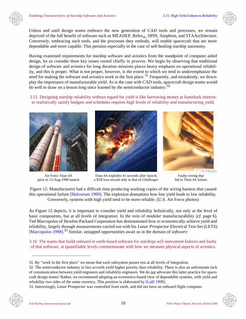
3.15 Designing starship reliability without regard for yield is like borrowing money at loanshark interest:to realistically satisfy budgets and schedules requires high levels of reliability and manufacturing yield.
As Figure 12 depicts, it is important to consider yield and reliability holistically, not only at the level ofbasic components, but at all levels of integration. In the vein of modular manufacturability (cf. page 6),Ted Marcopolus of Hewlett-Packard Corporation has demonstrated how to economically achieve yield andreliability, largely through measurements carried out with his Lunar Prospector Electrical Test-Set (LETS)[Marcopulos 1998].33 Similar, untapped opportunities await us in the domain of software:
3.16 The teams that build onboard or earth-based software for starships will instrument failures and faults of that software, at quantifiable levels commensurate with how we measure physical aspects of avionics.
31. By "work in the first place" we mean that each subsystem passes test at all levels of integration.32. The semiconductor industry in fact accords yield higher priority than reliability. There is also an unfortunate lackof communication between yield engineers and reliability engineers. We do not advocate this latter practice for space-craft design teams! Rather, we recommend adopting an economics-based view of dependable systems, with yield andreliability two sides of the same currency. This position is elaborated by [Lalli 1998].
Figure 12: Manufacturers had a difficult time producing working copies of the wiring harness that caused this operational failure [Halvorson 1999]. The explosion dramatizes how low yield leads to low reliability.
Conversely, systems with high yield tend to be more reliable. (U.S. Air Force photos)
33. Interestingly, Lunar Prospector was controlled from earth, and did not have an onboard flight computer.
Metal-to-metalshort circuit in SRAM
Pinhole defect inDRAM gate oxide
Air Force Titan 4A Titan 4A explodes 41 seconds after launch, Faulty wiring thatled to Titan 4A failureprior to 12-Aug-1998 launch a $1B loss second only to that of Challenger
Enabling Characteristics of Starship Software 3.16. Measure Those Failures and Faults!
Self-Healing Autonomous Spacecraft 19 NIAC Phase I Report, Revision 28-Feb-2000
As with hardware, software systems tend to be more reliable if they begin their operational life with fewerfaults ([Koshgoftaar et al 1998] p. 71). Avoidance is, and will remain, the most economical approach tohandling software faults ([Siewiorek and Swarz 1982], Chap. 3).34 Furthermore, a great deal – perhapsmost – of the complexity of a starship will be encompassed by its onboard and earth-based software. Forelectronics we measure, in excruciating detail, quantities such as current leakage, doping concentrations,and variations in oxide thickness [Bendetto 1998], [Runyon 1999], [Taur 1999], [Zorian 1999]. Thesequantities guide changes to our development processes – changes which converge on hardware that is suit-able for operation. In the case of software, however, we have yet to deploy instrumentation that quantifiesthe relation between failures and faults, faults and their root causes [Glass 1997].35 The viability of star-ship software depends on possessing, and taking advantage of, such instrumentation [Meyer 1999].
For illustration, suppose that we observe 100 mission-critical failures in the software module responsiblefor sending science data to earth. Further suppose that, over the same development cycle, we observe 10mission-critical failures in the software module that manages the distribution of spacecraft power. At firstblush, the order of magnitude difference in module failure rates suggests that we better spend more projectdollars testing communication software. But wait! This line of reasoning is based on the tacit assumptionthat the two modules are of comparable complexity, and that they have been subjected to testing at approx-imately the same level of intensity. If these assumptions do not hold, then uncovering, say, 95% of mis-sion-critical faults in communication software could cost much less than uncovering 95% of mission-critical faults in the power distribution software. In this case, we would do better to spend more projectdollars testing power distribution software. To effect a decision that accounts for all of these factors, weneed a predictive model that tells us how to minimize the test intensity (cost), while maintaining, say, 95%fault coverage (benefit), as a function of application complexity (independent variable). Alternatively,such a relation can help us predict the fault coverage, as a function of application complexity and testintensity. The benefit of such a predictive model is born out in the avoidance of software design faults.
To develop such a predictive model, we need to instrument the software development process in order to1) trace failures from the point at which they are observed to the point at which the underlying fault(s)were inserted into the system; 2) measure the evolving complexity of the application software; 3) quantify
34. It is in general much more expensive to tolerate latent software faults that manifest in situ.35. An unmanned NASA mission may have as many as three separate problem reporting and tracking systems; e.g.,software only (PFR), mission level (PR), and "institutional" (FR). As intimated by the caption to Figure 13, such sys-tems do not at present satisfy requirements for quantitatively instrumenting software failures and faults.
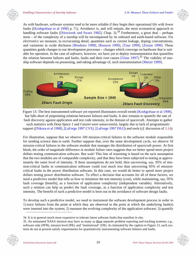
Figure 13: The best instrumented software yet reported illuminates overall trends [Koshgoftaar et al 1998], but falls short of pinpointing relations between failures and faults. It also remains to quantify the rate of
fault discovery against application and test code intensity, in the domain of spacecraft. Attempts to gather such statistics with Deep Space 1 and Cassini were unsuccessful, largely due to lack of programmatic
support ([Nikora et al 1998], [LaForge 1997 CVS], [LaForge 1997 DS1]) and tools (cf. discussion of 3.14).
Sam ple Size = 1940
A rchitec tu re5% D esign
27%
C oding68%
JStars Fault Orig in
D esign1%
C ode/test2% O ther
5%
In tegration69%
A cceptance23%
JStars Fault D iscovery
Enabling Characteristics of Starship Software and Avionics 3.17. Programmatic Support Bolsters Breakthroughs
Self-Healing Autonomous Spacecraft 20 NIAC Phase I Report, Revision 28-Feb-2000
the rate, type, and severity of faults; and 4) quantify test intensity and the way it changes over time [Mun-son and Werries 1996]. Patterns between failures, faults, program structure, and test intensity will emerge,and the fidelity of our model will continually improve [Nikora et al 1998]. At a tactical level, such workwill enable engineers and managers to answer questions such as: How many faults are there? In what mod-ules are the faults? How quickly are they being removed? Where should fault removal efforts be applied,and to what extent? Refer to Figure 13. The Army/Air Force Joint Surveillance Target Attack Radar Sys-tem (JStars) appears to be the only project for which a significant volume of such data, coarse-grained as itis, has been reported ([Koshgoftaar et al 1998], [Voas et al 1997] "data elusive"). Development of aninstrumented software model, and its application to work we propose for Phase II, would synergisticallybenefit starship autonomy.
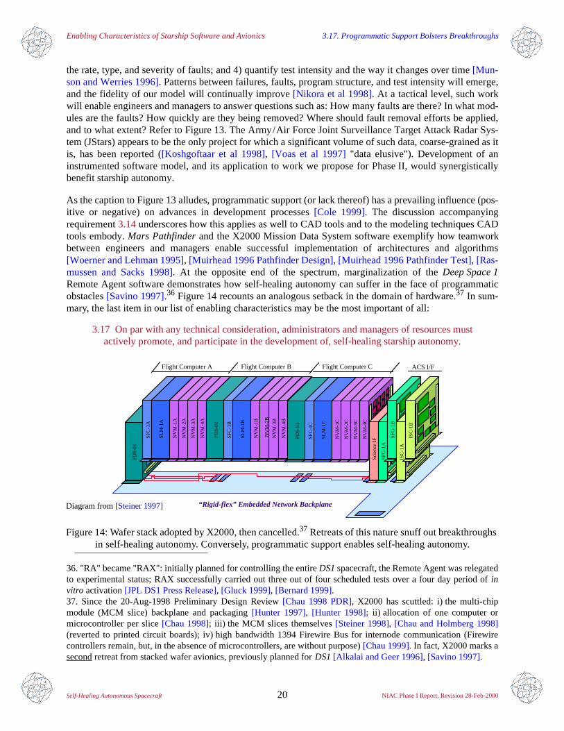
As the caption to Figure 13 alludes, programmatic support (or lack thereof) has a prevailing influence (pos-itive or negative) on advances in development processes [Cole 1999]. The discussion accompanyingrequirement 3.14 underscores how this applies as well to CAD tools and to the modeling techniques CADtools embody. Mars Pathfinder and the X2000 Mission Data System software exemplify how teamworkbetween engineers and managers enable successful implementation of architectures and algorithms[Woerner and Lehman 1995], [Muirhead 1996 Pathfinder Design], [Muirhead 1996 Pathfinder Test], [Ras-mussen and Sacks 1998]. At the opposite end of the spectrum, marginalization of the Deep Space 1Remote Agent software demonstrates how self-healing autonomy can suffer in the face of programmaticobstacles [Savino 1997].36 Figure 14 recounts an analogous setback in the domain of hardware.37 In sum-mary, the last item in our list of enabling characteristics may be the most important of all:
3.17 On par with any technical consideration, administrators and managers of resources mustactively promote, and participate in the development of, self-healing starship autonomy.
36. "RA" became "RAX": initially planned for controlling the entire DS1 spacecraft, the Remote Agent was relegatedto experimental status; RAX successfully carried out three out of four scheduled tests over a four day period of invitro activation [JPL DS1 Press Release], [Gluck 1999], [Bernard 1999].37. Since the 20-Aug-1998 Preliminary Design Review [Chau 1998 PDR], X2000 has scuttled: i) the multi-chipmodule (MCM slice) backplane and packaging [Hunter 1997], [Hunter 1998]; ii) allocation of one computer ormicrocontroller per slice [Chau 1998]; iii) the MCM slices themselves [Steiner 1998], [Chau and Holmberg 1998](reverted to printed circuit boards); iv) high bandwidth 1394 Firewire Bus for internode communication (Firewirecontrollers remain, but, in the absence of microcontrollers, are without purpose) [Chau 1999]. In fact, X2000 marks asecond retreat from stacked wafer avionics, previously planned for DS1 [Alkalai and Geer 1996], [Savino 1997].
Figure 14: Wafer stack adopted by X2000, then cancelled.37 Retreats of this nature snuff out breakthroughs in self-healing autonomy. Conversely, programmatic support enables self-healing autonomy.
“Rigid-flex” Embedded Network Backplane
PD
S-0
1
SF
C-1
A
I/f lo
gic
SL
M-1
A
NV
M-1
A
NV
M-2
A
NV
M-3
A
NV
M-4
A
Flight Computer A
PD
S-0
2
SF
C-1
B
I/f lo
gic
SL
M-1
B
NV
M-1
B
NV
M-2
B
NV
M-3
B
NV
M-4
B
Flight Computer B
PD
S-0
3
SF
C-1
C
I/f lo
gic
SL
M-1
C
NV
M-1
C
NV
M-2
C
NV
M-3
C
NV
M-4
CFlight Computer C
Sci
en
ce I
F
SF
G-1
A
SF
G-1
B
ISC
-1A
ISC
-1B
ACS I/F
Diagram from [Steiner 1997]
4. Advances in Self-Healing Architectures and Algorithms Highlights of Findings and Results
Self-Healing Autonomous Spacecraft 21 NIAC Phase I Report, Revision 28-Feb-2000
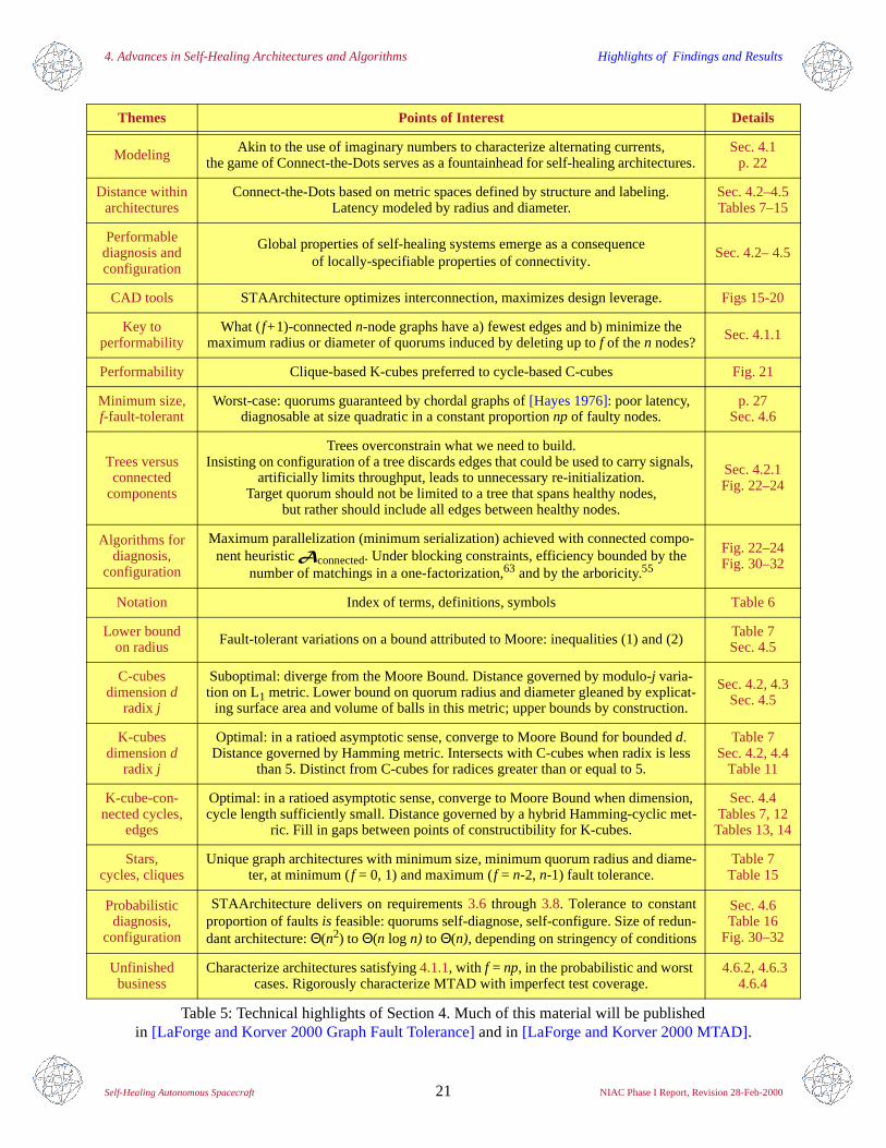
Themes Points of Interest Details
Modeling Akin to the use of imaginary numbers to characterize alternating currents,the game of Connect-the-Dots serves as a fountainhead for self-healing architectures.
Sec. 4.1p. 22
Distance withinarchitectures
Connect-the-Dots based on metric spaces defined by structure and labeling.Latency modeled by radius and diameter.
Sec. 4.2–4.5Tables 7–15
Performablediagnosis and configuration
Global properties of self-healing systems emerge as a consequenceof locally-specifiable properties of connectivity.
Sec. 4.2– 4.5
CAD tools STAArchitecture optimizes interconnection, maximizes design leverage. Figs 15-20
Key toperformability
What (f+1)-connected n-node graphs have a) fewest edges and b) minimize the maximum radius or diameter of quorums induced by deleting up to f of the n nodes? Sec. 4.1.1
Performability Clique-based K-cubes preferred to cycle-based C-cubes Fig. 21
Minimum size,f-fault-tolerant
Worst-case: quorums guaranteed by chordal graphs of [Hayes 1976]: poor latency, diagnosable at size quadratic in a constant proportion np of faulty nodes.
p. 27Sec. 4.6
Trees versusconnected
components
Trees overconstrain what we need to build.Insisting on configuration of a tree discards edges that could be used to carry signals,
artificially limits throughput, leads to unnecessary re-initialization.Target quorum should not be limited to a tree that spans healthy nodes,
but rather should include all edges between healthy nodes.
Sec. 4.2.1Fig. 22–24
Algorithms fordiagnosis,
configuration
Maximum parallelization (minimum serialization) achieved with connected compo-nent heuristic $connected. Under blocking constraints, efficiency bounded by the
number of matchings in a one-factorization,63 and by the arboricity.55
Fig. 22–24Fig. 30–32
Notation Index of terms, definitions, symbols Table 6
Lower boundon radius Fault-tolerant variations on a bound attributed to Moore: inequalities (1) and (2) Table 7
Sec. 4.5
C-cubesdimension d
radix j
Suboptimal: diverge from the Moore Bound. Distance governed by modulo-j varia-tion on L1 metric. Lower bound on quorum radius and diameter gleaned by explicat-
ing surface area and volume of balls in this metric; upper bounds by construction.
Sec. 4.2, 4.3Sec. 4.5
K-cubesdimension d
radix j
Optimal: in a ratioed asymptotic sense, converge to Moore Bound for bounded d. Distance governed by Hamming metric. Intersects with C-cubes when radix is less
than 5. Distinct from C-cubes for radices greater than or equal to 5.
Table 7Sec. 4.2, 4.4
Table 11
K-cube-con-nected cycles,
edges
Optimal: in a ratioed asymptotic sense, converge to Moore Bound when dimension, cycle length sufficiently small. Distance governed by a hybrid Hamming-cyclic met-
ric. Fill in gaps between points of constructibility for K-cubes.
Sec. 4.4Tables 7, 12Tables 13, 14
Stars,cycles, cliques
Unique graph architectures with minimum size, minimum quorum radius and diame-ter, at minimum (f = 0, 1) and maximum (f = n-2, n-1) fault tolerance.
Table 7Table 15
Probabilistic diagnosis,
configuration
STAArchitecture delivers on requirements 3.6 through 3.8. Tolerance to constantproportion of faults is feasible: quorums self-diagnose, self-configure. Size of redun-dant architecture: Θ(n2) to Θ(n log n) to Θ(n), depending on stringency of conditions
Sec. 4.6Table 16
Fig. 30–32
Unfinishedbusiness
Characterize architectures satisfying 4.1.1, with f = np, in the probabilistic and worst cases. Rigorously characterize MTAD with imperfect test coverage.
4.6.2, 4.6.34.6.4
Table 5: Technical highlights of Section 4. Much of this material will be publishedin [LaForge and Korver 2000 Graph Fault Tolerance] and in [LaForge and Korver 2000 MTAD].
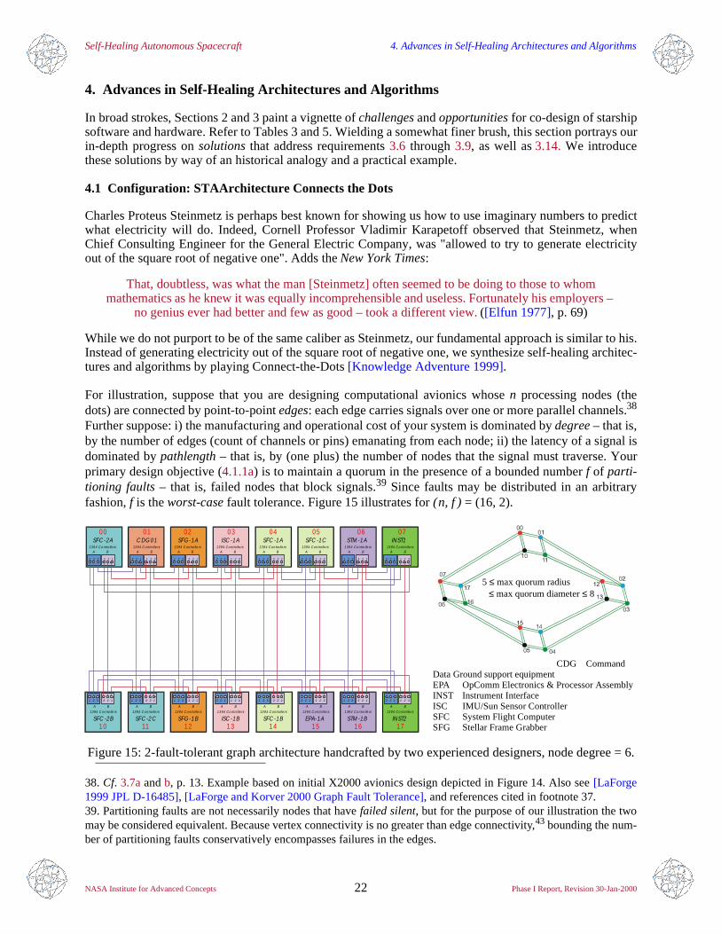
Self-Healing Autonomous Spacecraft 4. Advances in Self-Healing Architectures and Algorithms
NASA Institute for Advanced Concepts 22 Phase I Report, Revision 30-Jan-2000
4. Advances in Self-Healing Architectures and Algorithms
In broad strokes, Sections 2 and 3 paint a vignette of challenges and opportunities for co-design of starshipsoftware and hardware. Refer to Tables 3 and 5. Wielding a somewhat finer brush, this section portrays ourin-depth progress on solutions that address requirements 3.6 through 3.9, as well as3.14. We introducethese solutions by way of an historical analogy and a practical example.
4.1 Configuration: STAArchitecture Connects the Dots
Charles Proteus Steinmetz is perhaps best known for showing us how to use imaginary numbers to predictwhat electricity will do. Indeed, Cornell Professor Vladimir Karapetoff observed that Steinmetz, whenChief Consulting Engineer for the General Electric Company, was "allowed to try to generate electricityout of the square root of negative one". Adds the New York Times:
That, doubtless, was what the man [Steinmetz] often seemed to be doing to those to whommathematics as he knew it was equally incomprehensible and useless. Fortunately his employers –
no genius ever had better and few as good – took a different view. ([Elfun 1977], p. 69)
While we do not purport to be of the same caliber as Steinmetz, our fundamental approach is similar to his.Instead of generating electricity out of the square root of negative one, we synthesize self-healing architec-tures and algorithms by playing Connect-the-Dots [Knowledge Adventure 1999].
For illustration, suppose that you are designing computational avionics whose n processing nodes (thedots) are connected by point-to-point edges: each edge carries signals over one or more parallel channels.38
Further suppose: i) the manufacturing and operational cost of your system is dominated by degree – that is,by the number of edges (count of channels or pins) emanating from each node; ii) the latency of a signal isdominated by pathlength – that is, by (one plus) the number of nodes that the signal must traverse. Yourprimary design objective (4.1.1a) is to maintain a quorum in the presence of a bounded number f of parti-tioning faults – that is, failed nodes that block signals.39 Since faults may be distributed in an arbitraryfashion, f is the worst-case fault tolerance. Figure15 illustrates for (n, f ) = (16, 2).
38. Cf. 3.7a and b, p. 13. Example based on initial X2000 avionics design depicted in Figure 14. Also see [LaForge1999 JPL D-16485], [LaForge and Korver 2000 Graph Fault Tolerance], and references cited in footnote 37.39. Partitioning faults are not necessarily nodes that have failed silent, but for the purpose of our illustration the twomay be considered equivalent. Because vertex connectivity is no greater than edge connectivity,43 bounding the num-ber of partitioning faults conservatively encompasses failures in the edges.
Figure 15: 2-fault-tolerant graph architecture handcrafted by two experienced designers, node degree = 6.
SFC -1A
1 2 3
STM -1A
1 2 3
SFC -1C
3 2 1
INST1
3 2 1
SFG -1A
1 2 3
ISC -1A
3 2 1
C DG 01
3 2 1
SFC -1B
1 2 3
STM -1B
1 2 3
EPA-1A
3 2 1
INST2
3 2 1
SFG -1 B
1 2 3
ISC -1B
3 2 1
SFC -2A
1 2 3
SFC -2B
1 2 3
SFC -2 C
1 2 3
1394 C o ntro lle rsA B
1394 C on tro lle rsA B
1394 C on tro lle rsA B
1394 C o ntro lle rsA B
1394 C on tro lle rsA B
1394 C on tro lle rsA B
1394 C o ntro lle rsA B
1394 C o n tro lle rsA B
1394 C on tro lle rsA B
1394 C on tro lle rsA B
1394 C on tro lle rsA B
1394 C o ntro lle rsA B
1394 C on tro lle rsA B
1394 C on tro lle rsA B
1394 C o ntro lle rsA B
1394 C o n tro lle rsA B
3 2 1 3 2 11 2 3 1 2 33 2 1 1 2 31 2 3
3 2 1 3 2 11 2 3 1 2 33 2 1 1 2 3
3 2 1
3 2 1 3 2 1
00 01 02 03 04 05 06 07
10 11 12 13 14 15 16 17
CDG Command Data Ground support equipmentEPA OpComm Electronics & Processor AssemblyINST Instrument InterfaceISC IMU/Sun Sensor ControllerSFC System Flight ComputerSFG Stellar Frame Grabber
≤ max quorum diameter≤ 8 5 ≤ max quorum radius
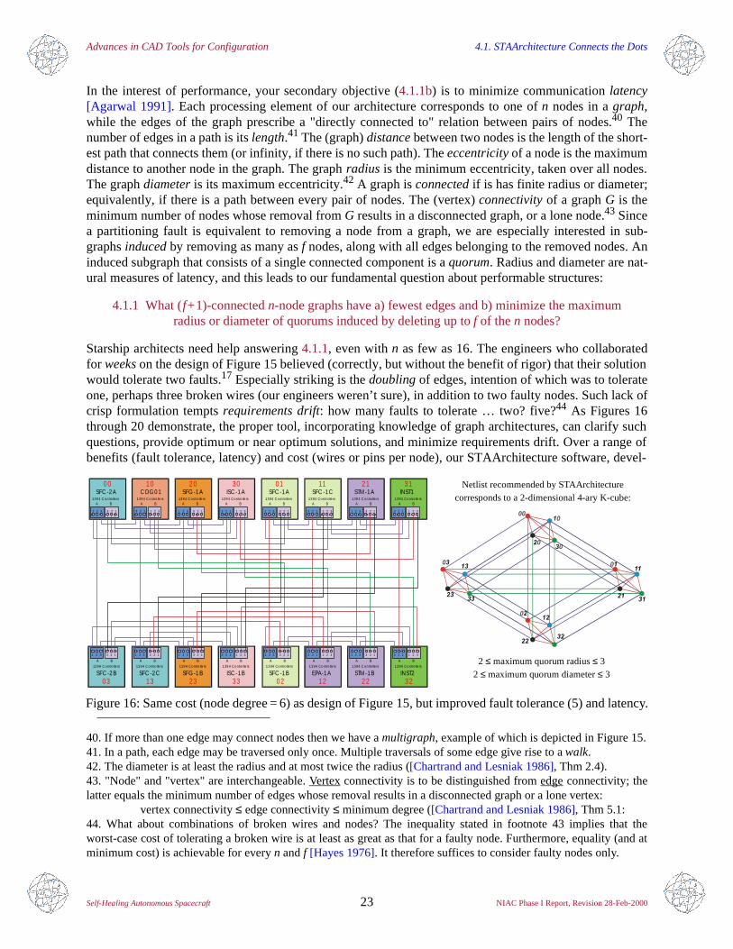
Advances in CAD Tools for Configuration 4.1. STAArchitecture Connects the Dots
Self-Healing Autonomous Spacecraft 23 NIAC Phase I Report, Revision 28-Feb-2000
In the interest of performance, your secondary objective (4.1.1b) is to minimize communication latency[Agarwal 1991]. Each processing element of our architecture corresponds to one of n nodes in a graph,while the edges of the graph prescribe a "directly connected to" relation between pairs of nodes.40 Thenumber of edges in a path is its length.41 The (graph) distance between two nodes is the length of the short-est path that connects them (or infinity, if there is no such path). The eccentricity of a node is the maximumdistance to another node in the graph. The graph radius is the minimum eccentricity, taken over all nodes.The graph diameter is its maximum eccentricity.42 A graph is connected if is has finite radius or diameter;equivalently, if there is a path between every pair of nodes. The (vertex) connectivity of a graph G is theminimum number of nodes whose removal from G results in a disconnected graph, or a lone node.43 Sincea partitioning fault is equivalent to removing a node from a graph, we are especially interested in sub-graphs induced by removing as many as f nodes, along with all edges belonging to the removed nodes. Aninduced subgraph that consists of a single connected component is a quorum. Radius and diameter are nat-ural measures of latency, and this leads to our fundamental question about performable structures:
4.1.1 What (f+1)-connected n-node graphs have a) fewest edges and b) minimize the maximumradius or diameter of quorums induced by deleting up to f of the n nodes?
Starship architects need help answering 4.1.1, even with n as few as 16. The engineers who collaboratedfor weeks on the design of Figure 15 believed (correctly, but without the benefit of rigor) that their solutionwould tolerate two faults.17 Especially striking is the doubling of edges, intention of which was to tolerateone, perhaps three broken wires (our engineers weren’t sure), in addition to two faulty nodes. Such lack ofcrisp formulation tempts requirements drift: how many faults to tolerate … two? five?44 As Figures 16through 20 demonstrate, the proper tool, incorporating knowledge of graph architectures, can clarify suchquestions, provide optimum or near optimum solutions, and minimize requirements drift. Over a range ofbenefits (fault tolerance, latency) and cost (wires or pins per node), our STAArchitecture software, devel-
40. If more than one edge may connect nodes then we have a multigraph, example of which is depicted in Figure 15.41. In a path, each edge may be traversed only once. Multiple traversals of some edge give rise to a walk.42. The diameter is at least the radius and at most twice the radius ([Chartrand and Lesniak 1986], Thm 2.4).43. "Node" and "vertex" are interchangeable. Vertex connectivity is to be distinguished from edge connectivity; thelatter equals the minimum number of edges whose removal results in a disconnected graph or a lone vertex:
vertex connectivity ≤ edge connectivity ≤ minimum degree ([Chartrand and Lesniak 1986], Thm 5.1:44. What about combinations of broken wires and nodes? The inequality stated in footnote 43 implies that theworst-case cost of tolerating a broken wire is at least as great as that for a faulty node. Furthermore, equality (and atminimum cost) is achievable for every n and f [Hayes 1976]. It therefore suffices to consider faulty nodes only.
Figure 16: Same cost (node degree = 6) as design of Figure 15, but improved fault tolerance (5) and latency.
SFC -1A
1 2 3
STM -1A
1 2 3
SFC -1C
3 2 1
INST1
3 2 1
SFG -1A
1 2 3
ISC -1 A
3 2 1
C DG 0 1
3 2 1
SFC -1B
1 2 3
STM -1B
1 2 3
EPA-1A
3 2 1
INST2
3 2 1
SFG -1 B
1 2 3
ISC -1B
3 2 1
SFC -2A
1 2 3
SFC -2 B
1 2 3
SFC -2C
1 2 3
1394 C o ntro lle rsA B
1394 C on tro lle rsA B
1394 C on tro lle rsA B
1394 C on tro lle rsA B
1394 C o ntro lle rsA B
1394 C o ntro lle rsA B
1394 C o ntro lle rsA B
1394 C o n tro lle rsA B
1394 C on tro lle rs
A B
1394 C on tro lle rs
A B
1394 C on tro lle rs
A B
1394 C on tro lle rs
A B
1394 C o ntro lle rs
A B
1394 C o ntro lle rs
A B
1394 C o ntro lle rs
A B
1394 C o n tro lle rs
A B
3 2 1 3 2 11 2 3 1 2 33 2 1 1 2 31 2 3
3 2 1 3 2 11 2 3 1 2 33 2 1 1 2 3
3 2 1
3 2 1 3 2 1
00 10 20 30 01 11 21 31
02 12 22 3203 13 23 33
Netlist recommended by STAArchitecturecorresponds to a 2-dimensional 4-ary K-cube:
2 ≤ maximum quorum radius≤ 3 2 ≤ maximum quorum diameter≤ 3
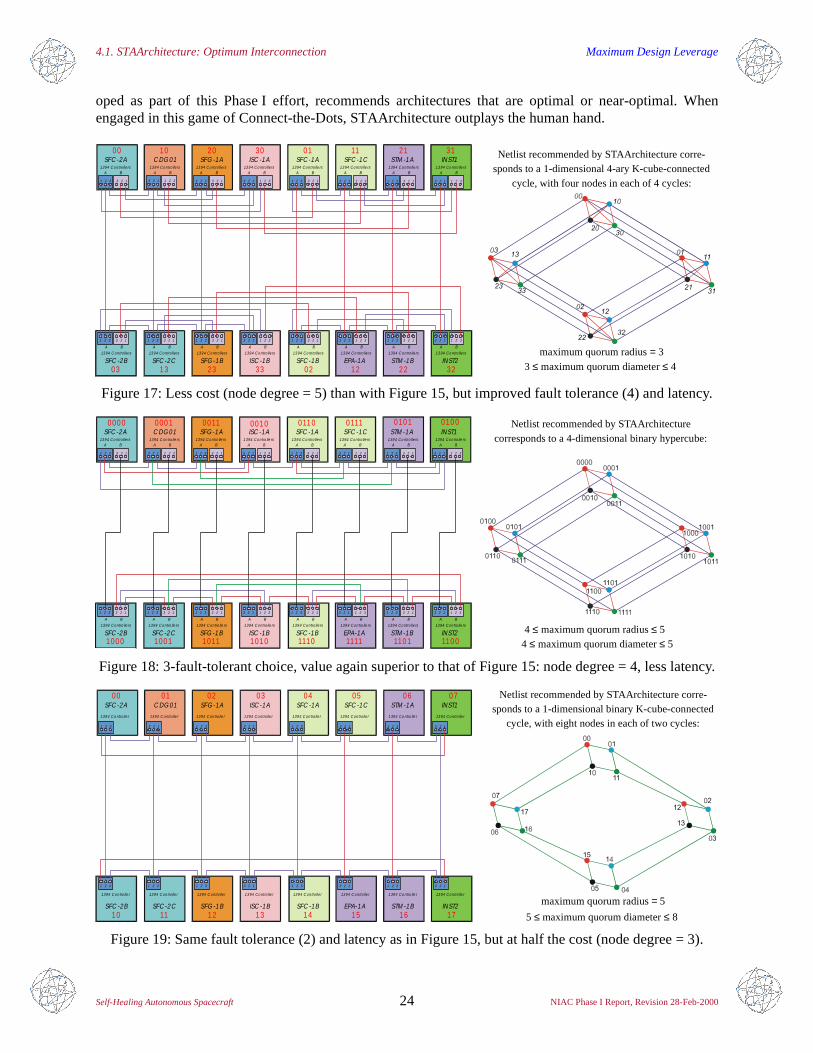
4.1. STAArchitecture: Optimum Interconnection Maximum Design Leverage
Self-Healing Autonomous Spacecraft 24 NIAC Phase I Report, Revision 28-Feb-2000
oped as part of this Phase I effort, recommends architectures that are optimal or near-optimal. Whenengaged in this game of Connect-the-Dots, STAArchitecture outplays the human hand.
Figure 17: Less cost (node degree = 5) than with Figure 15, but improved fault tolerance (4) and latency.
Figure 18: 3-fault-tolerant choice, value again superior to that of Figure 15: node degree = 4, less latency.
Figure 19: Same fault tolerance (2) and latency as in Figure 15, but at half the cost (node degree = 3).
SFC -1A
1 2 3
STM -1 A
1 2 3
SFC -1C
3 2 1
INST1
3 2 1
SFG -1A
1 2 3
ISC -1A
3 2 1
C DG 01
3 2 1
SFC -1B
1 2 3
STM -1B
1 2 3
EPA-1A
3 2 1
INST2
3 2 1
SFG -1B
1 2 3
ISC -1B
3 2 1
SFC -2A
1 2 3
SFC -2B
1 2 3
SFC -2C
1 2 3
1394 C o ntro lle rsA B
1394 C on tro lle rsA B
1394 C on tro lle rsA B
1394 C on tro lle rsA B
1394 C o ntro lle rsA B
1394 C o ntro lle rsA B
1394 C o ntro lle rsA B
1394 C o n tro lle rsA B
1394 C on tro lle rsA B
1394 C on tro lle rsA B
1394 C on tro lle rsA B
1394 C on tro lle rsA B
1394 C o ntro lle rsA B
1394 C o ntro lle rsA B
1394 C o ntro lle rsA B
1394 C o n tro lle rsA B
3 2 1 3 2 11 2 3 1 2 33 2 1 1 2 31 2 3
3 2 1 3 2 11 2 3 1 2 33 2 1 1 2 3
3 2 1
3 2 1 3 2 1
00 10 20 30 01 11 21 31
02 12 22 3203 13 23 33
Netlist recommended by STAArchitecture corre-sponds to a 1-dimensional 4-ary K-cube-connected
cycle, with four nodes in each of 4 cycles:
maximum quorum radius= 33 ≤ maximum quorum diameter≤ 4
4 ≤ maximum quorum radius≤ 5
Netlist recommended by STAArchitecturecorresponds to a 4-dimensional binary hypercube:
SFC -1A
1 2 3
STM -1A
1 2 3
SFC -1C
3 2 1
INST1
3 2 1
SFG -1A
1 2 3
ISC -1A
3 2 1
C DG 01
3 2 1
SFC -1B
1 2 3
STM -1B
1 2 3
EPA-1A
3 2 1
INST2
3 2 1
SFG -1 B
1 2 3
ISC -1B
3 2 1
SFC -2A
1 2 3
SFC -2B
1 2 3
SFC -2 C
1 2 3
1394 C o ntro lle rsA B
1394 C on tro lle rsA B
1394 C on tro lle rsA B
1394 C o ntro lle rsA B
1394 C on tro lle rsA B
1394 C on tro lle rsA B
1394 C o ntro lle rsA B
1394 C o n tro lle rsA B
1394 C on tro lle rsA B
1394 C on tro lle rsA B
1394 C on tro lle rsA B
1394 C o ntro lle rsA B
1394 C on tro lle rsA B
1394 C on tro lle rsA B
1394 C o ntro lle rsA B
1394 C o n tro lle rsA B
3 2 1 3 2 11 2 3 1 2 33 2 1 1 2 31 2 3
3 2 1 3 2 11 2 3 1 2 33 2 1 1 2 3
3 2 1
3 2 1 3 2 1
000 0 000 1 001 00011 010 0010 1011 0 0111
100 0 100 1 101 01011 110 0110 11110 1111 4 ≤ maximum quorum diameter≤ 5
5 ≤ maximum quorum diameter≤ 8
SFC -1A
1 2 3
STM -1A
1 2 3
SFC -1C
3 2 1
INST1
3 2 1
SFG -1A
1 2 3
ISC -1A
3 2 1
C DG 01
3 2 1
SFC -1B
1 2 3
STM -1B
1 2 3
EPA-1A
3 2 1
INST2
3 2 1
SFG -1 B
1 2 3
ISC -1B
3 2 1
SFC -2A
1 2 3
SFC -2B
1 2 3
SFC -2 C
1 2 3
1394 C o ntro lle r 1394 C on tro lle r 1394 C on tro lle r 1394 C o ntro lle r 1394 C on tro lle r 1394 C on tro lle r 1394 C o ntro lle r 1394 C o n tro lle r
1394 C on tro lle r 1394 C on tro lle r 1394 C on tro lle r 1394 C o ntro lle r 1394 C on tro lle r 1394 C on tro lle r 1394 C o ntro lle r 1394 C o n tro lle r
00 01 02 03 04 05 06 07
10 11 12 13 14 15 16 17
Netlist recommended by STAArchitecture corre-sponds to a 1-dimensional binary K-cube-connected
cycle, with eight nodes in each of two cycles:
maximum quorum radius= 5
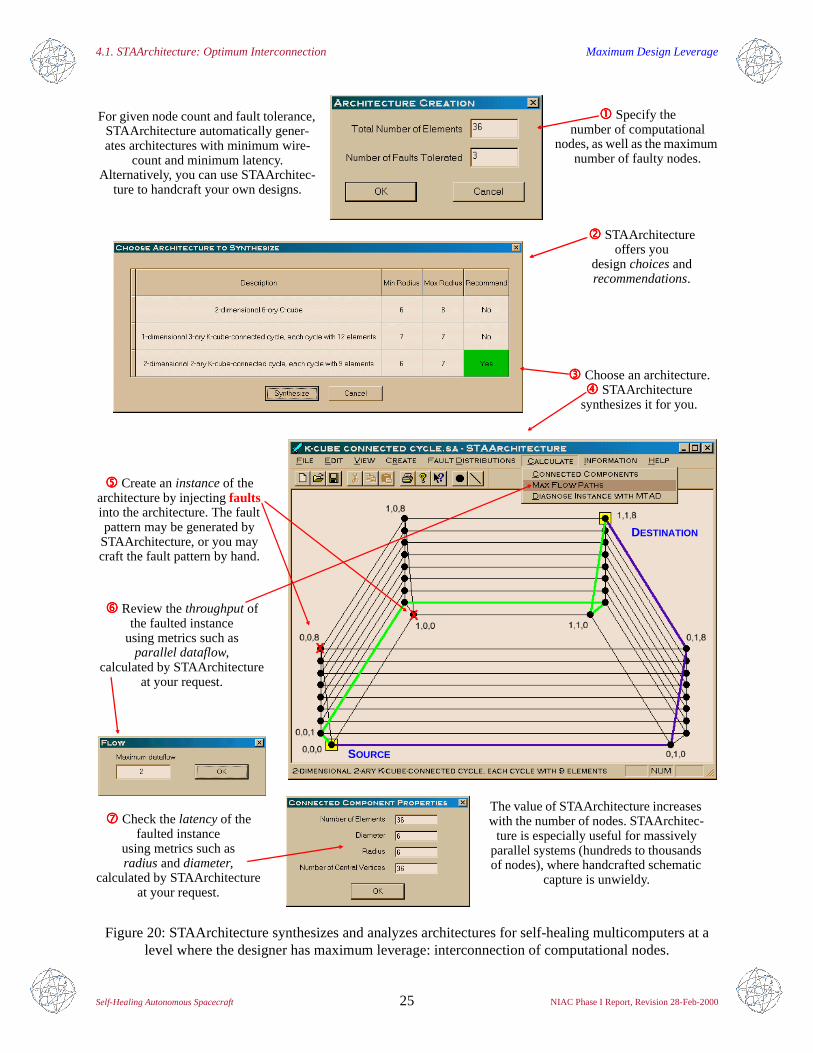
4.1. STAArchitecture: Optimum Interconnection Maximum Design Leverage
Self-Healing Autonomous Spacecraft 25 NIAC Phase I Report, Revision 28-Feb-2000
Figure 20: STAArchitecture synthesizes and analyzes architectures for self-healing multicomputers at a level where the designer has maximum leverage: interconnection of computational nodes.
cccc Specify thenumber of computational
nodes, as well as the maximum number of faulty nodes.
dddd STAArchitectureoffers you
design choices andrecommendations.
hhhh Review the throughput of the faulted instance
using metrics such asparallel dataflow,
calculated by STAArchitectureat your request.
iiii Check the latency of the faulted instance
using metrics such asradius and diameter,
calculated by STAArchitectureat your request.
eeee Choose an architecture.ffff STAArchitecture
synthesizes it for you.
For given node count and fault tolerance, STAArchitecture automatically gener-ates architectures with minimum wire-
count and minimum latency. Alternatively, you can use STAArchitec-
ture to handcraft your own designs.
gggg Create an instance of the architecture by injecting faults into the architecture. The fault pattern may be generated by STAArchitecture, or you may craft the fault pattern by hand.
The value of STAArchitecture increases with the number of nodes. STAArchitec-
ture is especially useful for massively parallel systems (hundreds to thousands of nodes), where handcrafted schematic
capture is unwieldy.
SOURCE
DESTINATION
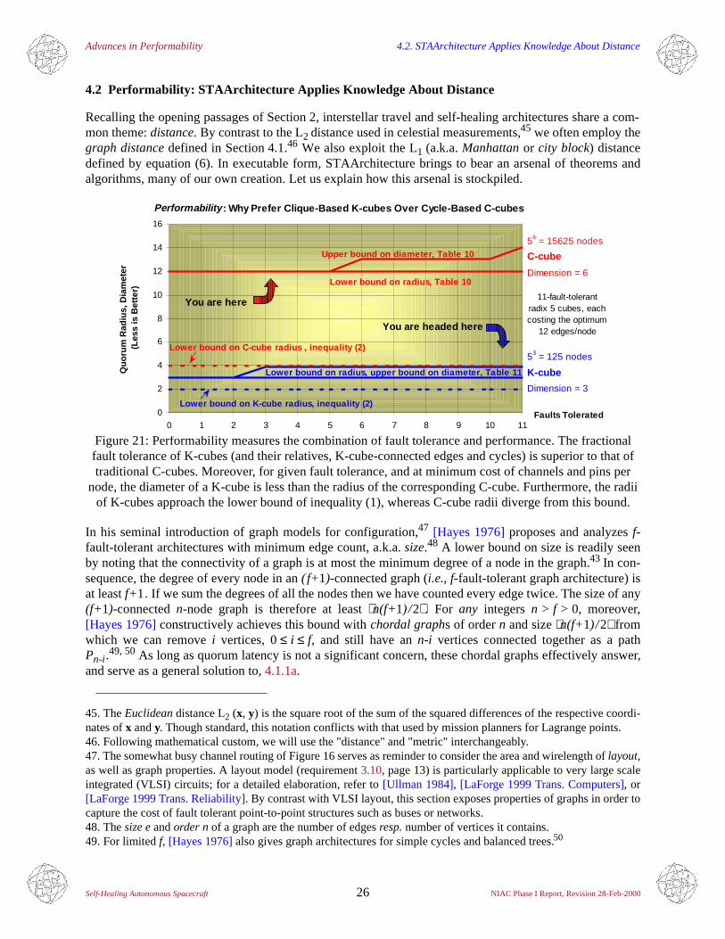
Advances in Performability 4.2. STAArchitecture Applies Knowledge About Distance
Self-Healing Autonomous Spacecraft 26 NIAC Phase I Report, Revision 28-Feb-2000
4.2 Performability: STAArchitecture Applies Knowledge About Distance
Recalling the opening passages of Section 2, interstellar travel and self-healing architectures share a com-mon theme: distance. By contrast to the L2 distance used in celestial measurements,45 we often employ thegraph distance defined in Section 4.1.46 We also exploit the L1 (a.k.a. Manhattan or city block) distancedefined by equation (6). In executable form, STAArchitecture brings to bear an arsenal of theorems andalgorithms, many of our own creation. Let us explain how this arsenal is stockpiled.
In his seminal introduction of graph models for configuration,47 [Hayes 1976] proposes and analyzes f-fault-tolerant architectures with minimum edge count, a.k.a. size.48 A lower bound on size is readily seenby noting that the connectivity of a graph is at most the minimum degree of a node in the graph.43 In con-sequence, the degree of every node in an ( f+1)-connected graph (i.e., f-fault-tolerant graph architecture) isat least f+1. If we sum the degrees of all the nodes then we have counted every edge twice. The size of any(f+1)-connected n-node graph is therefore at least n(f+1) /2 . For any integers n > f > 0, moreover,[Hayes 1976] constructively achieves this bound with chordal graphs of order n and size n(f+1)/2 fromwhich we can remove i vertices, 0≤ i ≤ f, and still have an n-i vertices connected together as a pathPn-i.
49, 50 As long as quorum latency is not a significant concern, these chordal graphs effectively answer,and serve as a general solution to, 4.1.1a.
45. The Euclidean distance L2 (x, y) is the square root of the sum of the squared differences of the respective coordi-nates of x and y. Though standard, this notation conflicts with that used by mission planners for Lagrange points.46. Following mathematical custom, we will use the "distance" and "metric" interchangeably.
Figure 21: Performability measures the combination of fault tolerance and performance. The fractional fault tolerance of K-cubes (and their relatives, K-cube-connected edges and cycles) is superior to that of traditional C-cubes. Moreover, for given fault tolerance, and at minimum cost of channels and pins per
node, the diameter of a K-cube is less than the radius of the corresponding C-cube. Furthermore, the radii of K-cubes approach the lower bound of inequality (1), whereas C-cube radii diverge from this bound.
47. The somewhat busy channel routing of Figure 16 serves as reminder to consider the area and wirelength of layout,as well as graph properties. A layout model (requirement 3.10, page 13) is particularly applicable to very large scaleintegrated (VLSI) circuits; for a detailed elaboration, refer to [Ullman 1984], [LaForge 1999 Trans. Computers], or[LaForge 1999 Trans. Reliability]. By contrast with VLSI layout, this section exposes properties of graphs in order tocapture the cost of fault tolerant point-to-point structures such as buses or networks.48. The size e and order n of a graph are the number of edges resp. number of vertices it contains.49. For limited f, [Hayes 1976] also gives graph architectures for simple cycles and balanced trees.50
Performability : Why Prefer Clique-Based K-cubes Over Cycle-Based C-cubes
0
2
4
6
8
10
12
14
16
0 1 2 3 4 5 6 7 8 9 10 11Faults Tolerated
Quo
rum
Rad
ius,
Dia
met
er(L
ess
is B
ette
r)
K-cube
You are here
C-cube
Dimension = 6
Dimension = 3
Upper bound on diameter, Table 1056 = 15625 nodes
53 = 125 nodes
Lower bound on radius, upper bound on diameter, Table 11
Lower bound on C-cube radius , ine qualit y (2)
Lower bound on K-cube radius, inequality (2)
You are headed here
11-fault-tolerant radix 5 cubes, each costing the optimum
12 edges/node
Lower bound on radius, Table 10
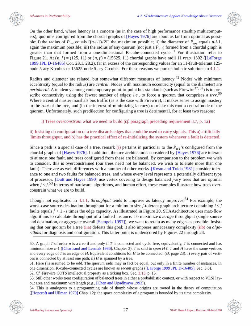
Advances in Performability 4.2. STAArchitecture Applies Knowledge About Distance
Self-Healing Autonomous Spacecraft 27 NIAC Phase I Report, Revision 28-Feb-2000
On the other hand, where latency is a concern (as in the case of high performance starship multicomput-ers), quorums configured from the chordal graphs of [Hayes 1976] are about as far from optimal as possi-ble: i) the radius of Pn-i equals (n-i-1)/2 , the maximum possible; ii) the diameter of Pn-i equals n-i-1,again the maximum possible; iii) the radius of any quorum (not just a Pn-i) formed from a chordal graph isgreater than that formed from a one-dimensional K-cube-connected cycle.51 For illustration refer toFigure 21. At (n, f ) = (125, 11) or (n, f ) = (15625, 11) chordal graphs have radii 11 resp. 1302 ([LaForge1999 JPL D-16485] Cor. 28.1, 28.2), far in excess of the corresponding values for an 11-fault-tolerant 125-node 5-ary K-cubes or 15625-node 5-ary C-cubes. For these reasons we pursue holistic solutions to 4.1.1.
Radius and diameter are related, but somewhat different measures of latency.42 Nodes with minimumeccentricity (equal to the radius) are central. Nodes with maximum eccentricity (equal to the diameter) areperipheral. A tendency among contemporary point-to-point bus standards (such as Firewire37, 52) is to pre-scribe connectivity using the fewest number of edges; i.e., to force a quorum that comprises a tree.50
Where a central master marshals bus traffic (as is the case with Firewire), it makes sense to assign masteryto the root of the tree, and (in the interest of minimizing latency) to make this root a central node of thequorum. Unfortunately, such predilection for configuring a tree is detrimental, for at least two reasons:
i) Trees overconstrain what we need to build (cf. paragraph preceding requirement 3.7, p. 12)
ii) Insisting on configuration of a tree discards edges that could be used to carry signals. This a) artificially limits throughput, and b) has the practical effect of re-initializing the system whenever a fault is detected.
Since a path is a special case of a tree, remark (i) pertains in particular to the Pn-i ’s configured from thechordal graphs of [Hayes 1976]. In addition, the tree architectures considered by [Hayes 1976] are tolerantto at most one fault, and trees configured from these are balanced. By comparison to the problem we wishto consider, this is overconstrained (our trees need not be balanced, we wish to tolerate more than onefault). There are as well differences with a number of other works. [Kwan and Toida 1981] consider toler-ance to one and two faults for balanced trees, and whose every level represents a potentially different typeof processor. [Dutt and Hayes 1990] use vertex covering to design balanced j-ary trees that are optimalwhen f < j .53 In terms of hardware, algorithms, and human effort, these examples illustrate how trees over-constrain what we are to build.
Though not explicated in 4.1.1, throughput tends to improve as latency improves.54 For example, theworst-case source-destination throughput for a minimum size f-tolerant graph architecture containing i ≤ ffaults equals f + 1 - i times the edge capacity. As illustrated in Figure 20, STAArchitecture uses max-flowalgorithms to calculate throughput of a faulted instance. To maximize average throughput (single sourceand destination, or aggregate overall [Sampels 1997]), we want to retain as many edges as possible. Insist-ing that our quorum be a tree (iia) defeats this goal; it also imposes unnecessary complexity (iib) on algo-rithms for diagnosis and configuration. This latter point is underscored by Figures 22 through 24.
50. A graph T of order n is a tree if and only if T is connected and cycle-free; equivalently, T is connected and hasminimum size n-1 ([Chartrand and Lesniak 1986], Chapter 3). T is said to span H if T and H have the same verticesand every edge of T is an edge of H. Equivalent conditions for H to be connected: (cf. page 23): i) every pair of verti-ces is connected by at least one path; ii)H is spanned by a tree.51. Here f is assumed to be odd. The quorum radii may in fact be equal, but only in a finite number of instances. Inone dimension, K-cube-connected cycles are known as secant graphs ([LaForge 1999 JPL D-16485], Sec. 3.6).52. Cf. Firewire COTS intellectual property as a ticking box, Sec. 3.13, p. 15.53. Still other works treat configuration of balanced trees in either a probabilistic context, or with respect to VLSI lay-out area and maximum wirelength (e.g., [Chen and Upadhyaya 1993]).54. This is analogous to a programming rule of thumb whose origins are rooted in the theory of computation([Hopcroft and Ullman 1979] Chap. 12): the space complexity of a program is bounded by its time complexity.
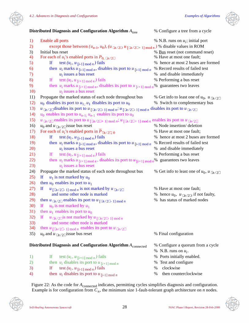
4.2. Advances in Diagnosis and Configuration Examples of Algorithms
Self-Healing Autonomous Spacecraft 28 NIAC Phase I Report, Revision 28-Feb-2000
Distributed Diagnosis and Configuration Algorithm Atree % Configure a tree from a cycle
1) Enable all ports % N.B. runs on ui ; initial port2) except those between (un-1, u0), (u n /2, u [n /2 + 1] mod n ) % disable values in ROM3) Initial bus reset % Bus reset (not command reset)4) For each of ui’s enabled ports in P0, n /2 % Have at most one fault;5) If test (ui , u [i-1] mod n ) fails % hence at most 2 buses are formed6) then ui marks u [i-1] mod n, disables its port to u [i-1] mod n % Record results of failed test7) ui issues a bus reset % and disable immediately8) If test (ui , u [i+ 1] mod n) fails % Performing a bus reset9) then ui marks u [i+ 1] mod n, disables its port to u [i+ 1] mod n% guarantees two leaves10) ui issues a bus reset11) Propagate the marked status of each node throughout bus % Get info to least one of u0, u n /212) u0 disables its port to u1; u1 disables its port to u0 % Switch to complementary bus13) u n / 2 disables its port to u [n /2 - 1] mod n; u [n /2 - 1] mod n disables its port to u n /214) u0 enables its port to un-1; un-1 enables its port to u015) u n /2 enables its port to u [n /2 + 1] mod n; u [n /2 + 1] mod n enables its port to u n /216) u0 and u n /2 issue bus reset % Node insertion/ deletion17) For each of ui’s enabled ports in Pn /2, 0 % Have at most one fault;18) If test (ui , u [i-1] mod n ) fails % hence at most 2 buses are formed19) then ui marks u [i-1] mod n, disables its port to u [i-1] mod n % Record results of failed test20) ui issues a bus reset % and disable immediately21) If test (ui , u [i+ 1] mod n) fails % Performing a bus reset22) then ui marks u [i+ 1] mod n , disables its port to u [i+ 1] mod n% guarantees two leaves23) ui issues a bus reset24) Propagate the marked status of each node throughout bus % Get info to least one of u0, u n /225) If u1 is not marked by u026) thenu0 enables its port to u127) If u [n /2 - 1] mod n is not marked by u n /2 % Have at most one fault;28) and some other node is marked % hence u0, u n /2, if not faulty,29) thenu n /2 enables its port to u [n /2 - 1] mod n % has status of marked nodes30) If u0 is not marked by u131) thenu1 enables its port to u032) If u n /2 is not marked by u [n /2 - 1] mod n33) and some other node is marked34) thenu [n /2 - 1] mod n enables its port to u n /235) u0 and u n /2 issue bus reset % Final configuration
Distributed Diagnosis and Configuration Algorithm Aconnected % Configure a quorum from a cycle% N.B. runs on ui .
1) If test (ui , u [i+1] mod n ) fails % Ports initially enabled.2) then ui disables its port to u [i+ 1] mod n % Test and configure3) If test (ui , u [i-1] mod n ) fails % clockwise4) then ui disables its port to u [i-1] mod n % then counterclockwise
Figure 22: As the code for Aconnected indicates, permitting cycles simplifies diagnosis and configuration. Example is for configuration from Cn, the minimum size 1-fault-tolerant graph architecture on n nodes.
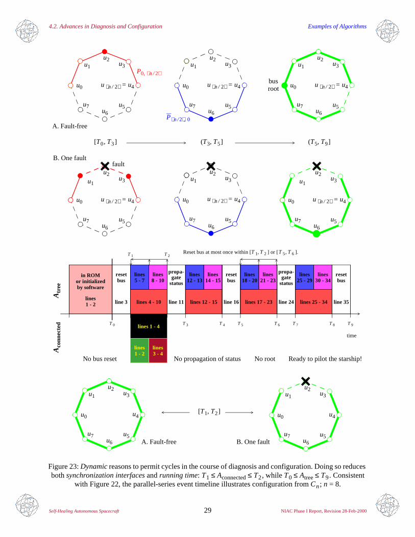
4.2. Advances in Diagnosis and Configuration Examples of Algorithms
Self-Healing Autonomous Spacecraft 29 NIAC Phase I Report, Revision 28-Feb-2000
Figure 23: Dynamic reasons to permit cycles in the course of diagnosis and configuration. Doing so reduces both synchronization interfaces and running time: T1 ≤ Aconnected≤ T2, while T0 ≤ Atree≤ T9. Consistent
with Figure 22, the parallel-series event timeline illustrates configuration from Cn; n = 8.
lines 1 - 4
Ready to pilot the starship!
lines lines3 - 41 - 2
linesline 3
lines lines8 - 105 - 7
lines 4 - 101 - 2 line 11
lines lines14 - 1512 - 13
lines 12 - 15 line 16
lines lines21 - 2318 - 20
lines 17 - 23 line 24
lines lines30 - 3425 - 29
lines 25 - 34 line 35
T 0
T 1 T 2
T 3 T 4 T 5 T 6 T 7 T 8 T 9
in ROMor initializedby software
time
resetbus
resetbus
resetbusgate
status
propa-gate
status
propa-
Reset bus at most once within [T 1, T 2 ] or [T 5, T 6 ].
Aco
nnec
ted
Atr
ee
No bus reset
P0, n /2
Pn /2, 0
bus u n / 2 = u4u0
u3u1
u2
u5u6
u7
u n / 2 = u4u0
u3u1
u2
u5u6
u7
u n / 2 = u4u0
u3u1
u2
u5u6
u7
u n / 2 = u4u0
u3u1
u2
u5u6
u7
u n / 2 = u4u0
u3u1
u2
u5u6
u7
u n / 2 = u4u0
u3u1
u2
u5u6
u7
fault
A. Fault-free
[T0, T3]
root
(T3, T5] (T5, T9]
B. One fault
u4u0
u3u1
u2
u5u6
u7
u4u0
u3u1
u2
u5u6
u7A. Fault-free
No root
B. One fault
[T1, T2]
No propagation of status
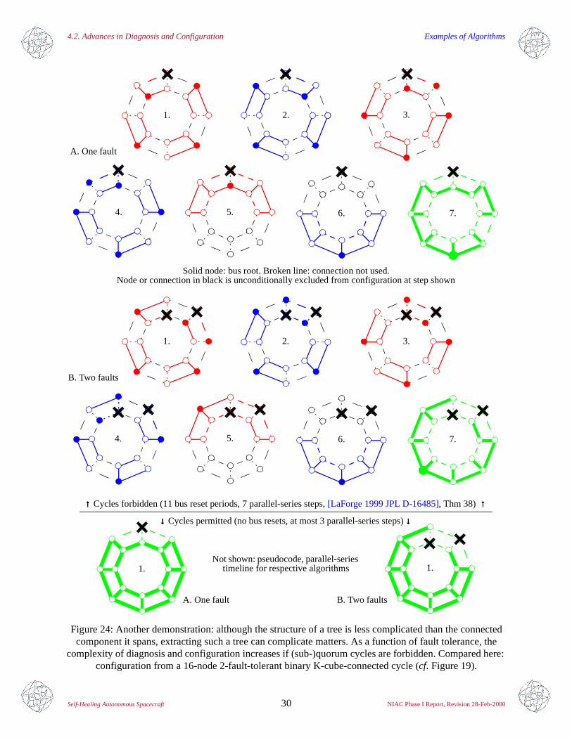
4.2. Advances in Diagnosis and Configuration Examples of Algorithms
Self-Healing Autonomous Spacecraft 30 NIAC Phase I Report, Revision 28-Feb-2000
Figure 24: Another demonstration: although the structure of a tree is less complicated than the connected component it spans, extracting such a tree can complicate matters. As a function of fault tolerance, the
complexity of diagnosis and configuration increases if (sub-)quorum cycles are forbidden. Compared here: configuration from a 16-node 2-fault-tolerant binary K-cube-connected cycle (cf. Figure 19).
1. 2. 3.
4. 5. 6. 7.
Solid node: bus root. Broken line: connection not used.Node or connection in black is unconditionally excluded from configuration at step shown
A. One fault
1. 2. 3.
B. Two faults
1. 1.
A. One fault B. Two faults
↑↑↑↑ Cycles forbidden (11 bus reset periods, 7 parallel-series steps, [LaForge 1999 JPL D-16485], Thm 38) ↑↑↑↑
↓↓↓↓ Cycles permitted (no bus resets, at most 3 parallel-series steps) ↓↓↓↓
4. 6. 7.5.
Not shown: pseudocode, parallel-series timeline for respective algorithms
4.2. Advances in Diagnosis and Configuration Quorums Should Include All Edges Between Healthy Nodes
Self-Healing Autonomous Spacecraft 31 NIAC Phase I Report, Revision 28-Feb-2000
Continuing from page 27, our pronounced elaboration of points (i) and (ii) is in part directed at stemmingthe cultural tide of trees as desiderata for quorums.55 While it is true that trees foster simplification of rout-ing algorithms,56 unbridled application of this fact undercuts performability. In summary:
4.2.1 The target quorum for self-healing architectures should not be limited to a tree that spanshealthy nodes, but rather should include all edges between healthy nodes.
Contrasting trees with connected components, we are now in a position to distinguish radius and diameter.Denote by H an arbitrary quorum induced by deleting i nodes of an n-node (f + 1)-connected graph G. If0 ≤ i ≤ f then this quorum is guaranteed to be connected, and therefore possesses one or more spanningtrees.50 Any tree has at most two central vertices, and they (it) always lie(s) at the intersection of maximumlength path(s). An immediate corollary is that the diameter of a tree is either twice its radius, or twice itsradius minus one ([LaForge 1999 JPL D-16485] Thm 1, Cor. 1.1). The power of this observation is bol-stered by a theorem of [Ore 1962]: for every node u of a connected graph H, there exists a spanning tree ofH that is distance-preserving from u. Moreover, we can compute, on a Turing machine equivalent and intime O(n(n+e)), a spanning tree having minimum radius ([LaForge 1999 JPL D-16485] Thm 36).48 Takentogether, these results imply that a there is a spanning tree of H whose radius is identical to that of H … thebest we could hope for. On the other hand, the diameter of this tree is equal to, or one less than, twice theradius … i.e., the worst-case latency is about as bad as it gets.42 By contrast, and as depicted in Figure 21,the quorum itself may have a diameter much smaller than twice the radius, even approaching the value ofthe radius itself. The highly performable structures synthesized by STAArchitecture exhibit this feature.For these reasons our analysis emphasizes radius.
Through the end of Section 4.5 we assume: i) faults have been correctly diagnosed; ii) the outcome of thisdiagnosis is passed to a configuration algorithm (which may be distributed, cf. Figures 22 through 24);iii) nodes (but not edges) may be faulty (i.e., deleted). Since edge connectivity is no less than vertex con-nectivity, item (iii) does not materially affect our analysis; however, allowing the deletion of edges canchange the sharpness of our results for radius and diameter.44 Refer Table 7. STAArchitecture’s candidatesfor configuration architectures are members of the set *+
n,f,k of minimum size (f+1)-connected graphs oforder n whose quorums, induced by deletion of up to f vertices, have radii at most k. For given n and f, wenaturally wish to assure that k is the exact minimum, in which case we write * n,f , perhaps with an extrasubscript k. We denote the corresponding radius by ρ(n, f ). Although the general solution to this problemappears to be unknown,57 we can enumerate * n,0,k=2, * n,1,k=n/2, and * n,n-2,k=2; that is, ρ(n, 0) = 2,ρ(n, 1) = n/2 , and ρ(n, n-2) = 1. For other values of f, we provide upper and lower bounds on ρ(n, f ),and give sets *+
n,f,k whose induced quorums have O(log n) radii.
55. The complexity illustrated by Figures 22 through 24 goes deeper than first appears. If one insists that each sub-quorum used to form a tree be cycle-free, then to cover all edges of the embedding architecture (i.e., test every possi-ble pairwise connection), we must factor the corresponding graph into forests of trees. The union of these forestscomprises the embedding architecture, and pairs of forests are edgewise disjoint. Under the constraint of cycle-freeconfiguration, the extent to which diagnosis and configuration can be parallelized is at least the minimum number offorests in any such factorization. This number is known as the aboricity of the graph, and can be calculated (albeitsomewhat awkwardly) by applying a result of Nash-Williams: Let em be the maximum size of any subgraph of order
m; the arboricity is the largest value of ([Bollabás, 1978], Thm 5.8). By contrast, a generalization
of our connected component algorithm (Figure 22) executes in a number of serial steps that is at most the maximumdegree of a node in the graph architecture. [LaForge 1994] illustrates application of matching and Hamiltonian cyclesto parallel scheduling of tests among nodes in locally spared arrays.56. As long as everything works properly, the simplification exploits the following property (which is, in fact, anequivalent definition of a tree): between any two nodes there is a unique path (cf. [Anderson 1998] Chap 13-17).
max1 m n≤ ≤em
m 1–-------------
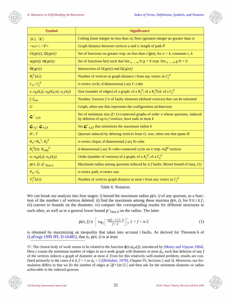
4. Advances in Self-Healing Architectures Index of Terms, Definitions, Symbols, and Notation
Self-Healing Autonomous Spacecraft 32 NIAC Phase I Report, Revision 28-Feb-2000
We can break our analysis into four stages: i) bound the maximum radius ρ(n, i) of any quorum, as a func-tion of the number i of vertices deleted; ii) find the maximum among these maxima ρ(n, i), for 0≤ i ≤ f ;iii) convert to bounds on the diameter; iv) compare the corresponding results for different structures toeach other, as well as to a general lower bound ρ–
Thm 6 on the radius. The latter
ρ(n, f) ≥ , 1 < f < n-2 (1)
is obtained by maximizing an inequality that takes into account i faults. As derived for Theorem 6 of[LaForge 1999 JPL D-16485], that is, ρ(n, i) is at least
57. The closest body of work seems to be related to the function ϕ(n,d0,d,f), introduced by [Murty and Vijayan 1964].Here j counts the minimum number of edges in an n-node graph with diameter at most d0, such that deletion of any fof the vertices induces a graph of diameter at most d. Even for this relatively well-studied problem, results are con-fined primarily to the cases d ≤ 4, f = 1 or d0 = 2 ([Bollabás, 1978], Chapter IV, Sections 2 and 3). Moreover, our for-mulation differs in that we fix the number of edges at (f+1)n/2 , and then ask for the minimum diameter or radiusachievable in the induced quorum.
Symbol Significance
x ; x Ceiling (least integer no less than x); floor (greatest integer no greater than x)
<u,v>; <P> Graph distance between vertices u and v; length of path P
O(g(n)); Ω(g(n)) Set of functions no greater resp. no less than c⋅g(n), for n > k, constants c, k
o(g(n)); ω(g(n)) Set of functions h(n) such that lim n → ∞ h/g = 0 resp. lim n → ∞ g/h = 0
Θ(g(n)) Intersection of O(g(n)) and Ω(g(n))
BjC(d,i) Number of vertices at graph distance i from any vertex in Cj
d
Cn; Cjd n-vertex cycle; d-dimensional j-ary C-cube
e, eK(d,j); eK(d,j,n); eC(d,j) Size (number of edges) of a graph; of a Kjd; of a Kj
d(n); of a Cjd
f, ffrac Number, fraction f /n of faulty elements (deleted vertices) that can be tolerated
G Graph, often one that represents the configuration architecture
* +n,f,k
Set of minimum size (f+1)-connected graphs of order n whose quorums, inducedby deletion of up to f vertices, have radii at most k
* n,f , * n,f,k Set *+n,f,k that minimizes the maximum radius k
H ; T Quorum induced by deleting vertices from G; tree, often one that spans H
Kn=Kn1; Kj
d n-vertex clique; d-dimensional j-ary K-cube
Kjd(n); KmÞj
d d-dimensional j-ary K-cube-connected cycle on n resp. m⋅j d vertices
n; nK(d,j); nC(d,j) Order (number of vertices) of a graph; of a Kjd; of a Cj
d
ρ(n, f); ρ–Thm 6 Maximum radius among quorums induced by ≤ f faults; Moore bound of ineq. (1)
Pn; Sn n-vertex path; n-vertex star
VjC(d,i) Number of vertices graph distance at most i from any vertex in Cj
d
Table 6: Notation.
logfn f 1–( ) 3+
f 2+----------------------------
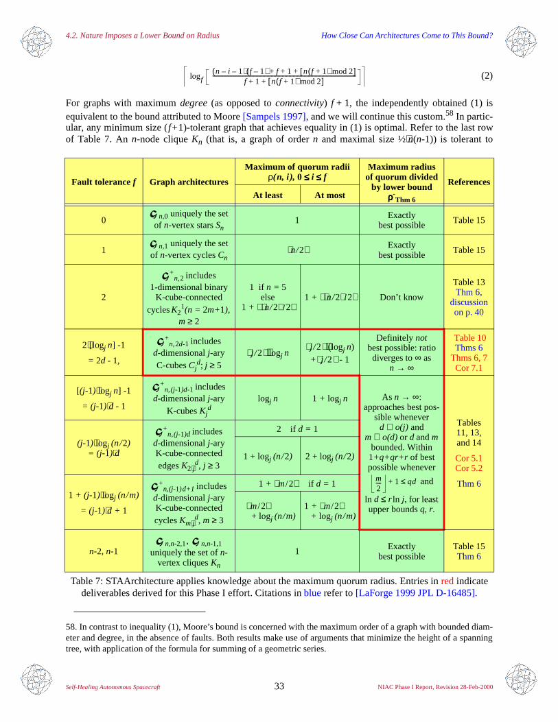
4.2. Nature Imposes a Lower Bound on Radius How Close Can Architectures Come to This Bound?
Self-Healing Autonomous Spacecraft 33 NIAC Phase I Report, Revision 28-Feb-2000
(2)
For graphs with maximum degree (as opposed to connectivity) f + 1, the independently obtained (1) isequivalent to the bound attributed to Moore [Sampels 1997], and we will continue this custom.58 In partic-ular, any minimum size (f+1)-tolerant graph that achieves equality in (1) is optimal. Refer to the last rowof Table 7. An n-node clique Kn (that is, a graph of order n and maximal size ½⋅n(n-1)) is tolerant to
58. In contrast to inequality (1), Moore’s bound is concerned with the maximum order of a graph with bounded diam-eter and degree, in the absence of faults. Both results make use of arguments that minimize the height of a spanningtree, with application of the formula for summing of a geometric series.
Fault tolerance f Graph architectures
Maximum of quorum radii ρ(n, i), 0 ≤≤≤≤ i ≤≤≤≤ f
Maximum radiusof quorum divided
by lower boundρρρρ-
Thm 6
References
At least At most
0* n,0 uniquely the set of n-vertex stars Sn
1 Exactlybest possible Table 15
1* n,1 uniquely the set of n-vertex cycles Cn
n/2 Exactlybest possible Table 15
2
*+n,2 includes
1-dimensional binary K-cube-connected
cycles K21(n = 2m+1), m ≥ 2
1 if n = 5else
1 + n/2 /21 + n/2 /2 Don’t know
Table 13 Thm 6,
discussionon p. 40
2⋅[logj n] -1
= 2d - 1,
*+n,2d-1 includes
d-dimensional j-aryC-cubes Cj
d; j ≥ 5 j / 2⋅logj n
j / 2⋅(logj n)
+ j / 2 - 1
Definitely notbest possible: ratiodiverges to ∞ as
n → ∞
Table 10 Thms 6
Thms 6, 7 Cor 7.1
[(j-1)⋅logj n] -1
= (j-1)⋅d - 1
*+n,(j-1)d-1 includes
d-dimensional j-aryK-cubes Kj
dlogj n 1 + logj n As n → ∞:
approaches best pos-sible whenever
d ∈ o(j) and m ∈ o(d) or d and m
bounded. Within 1+q+qr+r of best possible whenever
and
ln d ≤ r ln j, for least upper bounds q, r.
Tables11, 13,and 14
Cor 5.1Cor 5.2
Thm 6
(j-1)⋅logj (n/2)= (j- 1)⋅d
*+n,(j-1)d includes
d-dimensional j-aryK-cube-connected edges K2⋅j
d, j ≥ 3
2 if d = 1
1 + logj (n/2) 2 + logj (n/2)
1 + (j- 1)⋅logj (n/m)
= (j-1)⋅d + 1
*+n,(j-1)d+1 includes
d-dimensional j-aryK-cube-connected cycles Km⋅j
d, m ≥ 3
1 + m/2 if d = 1
m/2+ logj (n/m)
1 + m/2 + logj (n/m)
n-2, n-1*
n,n-2,1, * n,n-1,1
uniquely the set of n-vertex cliques Kn
1 Exactlybest possible
Table 15Thm 6
Table 7: STAArchitecture applies knowledge about the maximum quorum radius. Entries in red indicate deliverables derived for this Phase I effort. Citations in blue refer to [LaForge 1999 JPL D-16485].
logfn i– 1–( ) f 1–( ) f 1 n f 1+( ) mod 2[ ]+ + +
f 1 n f 1+( ) mod 2[ ]+ +---------------------------------------------------------------------------------------------------------
m2---- 1+ qd≤
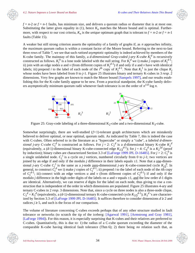
4.2. Nature Imposes a Lower Bound on Radius K-cubes and Their Relatives Attain This Bound
Self-Healing Autonomous Spacecraft 34 NIAC Phase I Report, Revision 28-Feb-2000
f = n-2 or f = n-1 faults, has minimum size, and delivers a quorum radius or diameter that is at most one.Substituting the latter gives equality in (1), hence Kn matches the Moore bound and is optimal. Further-more, with respect to our cost criteria, Kn is the unique optimum graph that is tolerant to f = n-2 or f = n-1faults (Table 15).
A weaker but still strong criterion asserts the optimality of a family of graphs if, as n approaches infinity,the maximum quorum radius is within a constant factor of the Moore bound. Referring to the next-to-lastthree rows of Table 7, we see that such ratioed asymptotic optimality is indeed achieved by members of theK-cube family. The mainstay of this family, a d-dimensional Gray-coded j-ary K-cube Kj
d is recursivelyconstructed as follows. Kj
0 is a lone node labeled with the null string. For Kjd we i) make j copies of Kj
d-1;ii) join with an edge nodes u and v (from different copies of Kj
d-1) if and only if u and v have with identicallabels; iii) prepend i to the label of each node of the ith copy of Kj
d-1. Note that Kj1 is just the clique Kj
whose nodes have been labeled from 0 to j-1. Figure 25 illustrates binary and ternary K-cubes in 3resp. 2dimensions. Very few graphs are known to match the Moore bound [Sampels 1997], and our results estab-lishing this for the K-cube family appear to be new. From a practical standpoint, the K-cube family deliv-ers asymptotically minimum quorum radii whenever fault tolerance is on the order of n1/d log n.
Somewhat surprisingly, there are well-studied (f+1)-tolerant graph architectures which are mistakenlybelieved to deliver optimal, or near optimal, quorum radii. As indicated by Table 7, this is indeed the casewith C-cubes. Often referred to in the literature as a "hypercube" or simply a "cube", a labeled d-dimen-sional j-ary C-cube Cj
d is constructed as follows. For j = 2: C2d is a d-dimensional binary K-cube K2
d
(equivalently, a (d-1)-dimensional binary K-cube-connected edge K2⋅2d-1); for j = 4: C4
d is a K22d (proof
by induction); binary cubes are characterized Section 3.3 of [LaForge 1999 JPL D-16485]. For j > 2: Cj0 is
a single unlabeled node. Cj1 is a cycle on j vertices, numbered circularly from 0 to j-1; two vertices are
joined by an edge if and only if the modulo j difference in their labels equals ±1. Note that a one-dimen-sional j-ary C-cube Cj
1 is the same as a j-node zero-dimensional j-ary K-cube-connected cycle Kj⋅j0. In
general, to construct Cjd we i) make j copies of Cj
d-1; ii) prepend i to the label of each node of the ith copyof Cj
d-1; iii) connect with an edge vertices u and v (from different copies of Cjd-1) if and only if the
moduloj difference in the high order digits of the labels on u and v equals ±1, and the low order d-1 digitsare identical. Alternatively, we can reserve d digits for the label on each node, thus giving to rise a con-struction that is independent of the order in which dimensions are populated. Figure 25 illustrates 4-ary andternary C-cubes in 2 resp. 3 dimensions. Note that, since a cycle on three nodes is also a three-node clique,C3
d = K3d (equivalently, a (d-1)-dimensional ternary K-cube-connected cycle K3⋅3
d-1); K3d ’s are character-
ized by Section 3.3 of [LaForge 1999 JPL D-16485]. It suffices therefore to consider dimensions d ≥ 2 andradices j ≥ 5, and such is the focus of our comparison.
The volume of literature concerning C-cubes exceeds perhaps that of any other structure studied in faulttolerance or networks (to scratch the tip of the iceberg: [Agarwal 1991], [Armstrong and Gray 1981],[LaForge 1994]). For this reason, it is especially surprising that K-cubes and their relatives are preferred toC-cubes. Quantitatively, this is due to: 1) the radius of a C-cube quorum exceeding the diameter of thecomparable K-cube having identical fault tolerance (Thm 6); 2) there being no relation such that, as
Figure 25: Gray-code labeling of a three-dimensional K2-cube and a two-dimensional K3-cube.02
00
01
12
10
11
22
20
21
K32K2
3
000 001
010 011
100 101
110 111
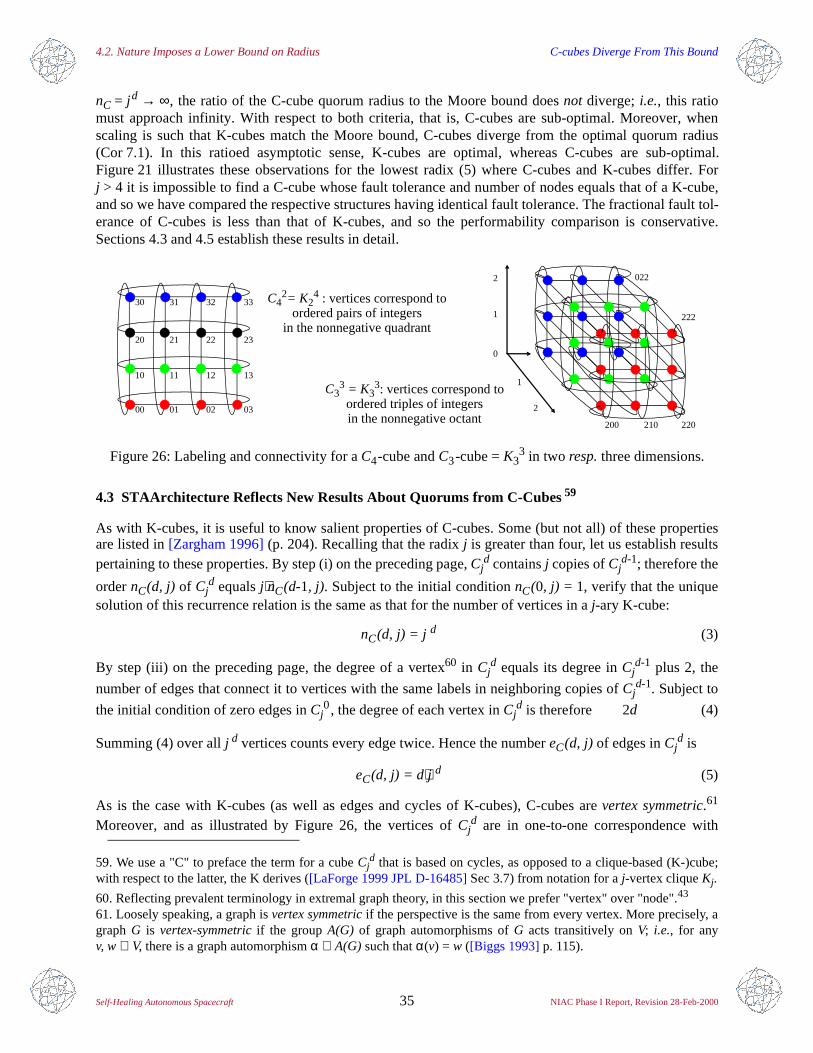
4.2. Nature Imposes a Lower Bound on Radius C-cubes Diverge From This Bound
Self-Healing Autonomous Spacecraft 35 NIAC Phase I Report, Revision 28-Feb-2000
nC = j d → ∞, the ratio of the C-cube quorum radius to the Moore bound does not diverge; i.e., this ratiomust approach infinity. With respect to both criteria, that is, C-cubes are sub-optimal. Moreover, whenscaling is such that K-cubes match the Moore bound, C-cubes diverge from the optimal quorum radius(Cor 7.1). In this ratioed asymptotic sense, K-cubes are optimal, whereas C-cubes are sub-optimal.Figure 21 illustrates these observations for the lowest radix (5) where C-cubes and K-cubes differ. Forj > 4 it is impossible to find a C-cube whose fault tolerance and number of nodes equals that of a K-cube,and so we have compared the respective structures having identical fault tolerance. The fractional fault tol-erance of C-cubes is less than that of K-cubes, and so the performability comparison is conservative.Sections 4.3 and 4.5 establish these results in detail.
4.3 STAArchitecture Reflects New Results About Quorums from C-Cubes59
As with K-cubes, it is useful to know salient properties of C-cubes. Some (but not all) of these propertiesare listed in [Zargham 1996] (p. 204). Recalling that the radix j is greater than four, let us establish resultspertaining to these properties. By step (i) on the preceding page, Cj
d contains j copies of Cjd-1; therefore the
order nC(d, j) of Cjd equals j⋅nC(d-1, j). Subject to the initial condition nC(0, j) = 1, verify that the unique
solution of this recurrence relation is the same as that for the number of vertices in a j-ary K-cube:
nC(d, j) = j d (3)
By step (iii) on the preceding page, the degree of a vertex60 in Cjd equals its degree in Cj
d-1 plus 2, the
number of edges that connect it to vertices with the same labels in neighboring copies of Cjd-1. Subject to
the initial condition of zero edges in Cj0, the degree of each vertex in Cj
d is therefore 2d (4)
Summing (4) over all j d vertices counts every edge twice. Hence the number eC(d, j) of edges in Cjd is
eC(d, j) = d⋅j d (5)
As is the case with K-cubes (as well as edges and cycles of K-cubes), C-cubes are vertex symmetric.61
Moreover, and as illustrated by Figure 26, the vertices of Cjd are in one-to-one correspondence with
Figure 26: Labeling and connectivity for a C4-cube and C3-cube =K33 in two resp. three dimensions.
59. We use a "C" to preface the term for a cube Cjd that is based on cycles, as opposed to a clique-based (K-)cube;
with respect to the latter, the K derives ([LaForge 1999 JPL D-16485] Sec 3.7) from notation for a j-vertex clique Kj.
60. Reflecting prevalent terminology in extremal graph theory, in this section we prefer "vertex" over "node".43
61. Loosely speaking, a graph is vertex symmetric if the perspective is the same from every vertex. More precisely, agraph G is vertex-symmetric if the group A(G) of graph automorphisms of G acts transitively on V; i.e., for anyv, w∈ V, there is a graph automorphism α ∈ A(G) such that α(v) = w ([Biggs 1993] p. 115).
03
C42= K2
4 : vertices correspond toordered pairs of integers
C33 = K3
3: vertices correspond toordered triples of integers
in the nonnegative quadrant
in the nonnegative octant
13
23
33
02
12
22
32
01
11
21
31
00
10
20
30
2
1
0
1
2
220210200
222
022
Advances in Self-Healing Architectures 4.3. STAArchitecture Reflects New Results About Quorums from C-cubes
Self-Healing Autonomous Spacecraft 36 NIAC Phase I Report, Revision 28-Feb-2000
ordered d-tuples, each of whose coordinates is a nonnegative integer. This suggests that, if two verticesu = (ud-1, … , u0) and v = (vd-1, … , v0) are sufficiently close, their distance should be given by the L1
metric (also known as the city block, or Manhattan metric): (6)
This tendency is born out by the L1 "modulo j" metric of (7). If u and v are vertices of Kjd, Gray-code
labeled according to steps (i) – (iii) on page 34, then <u, v> equals the number of digits where the respec-tive labels for u and v are different ([LaForge 1999 JPL D-16485] Thm 7). The analog for C-cubes:
Theorem 1. If u and v are vertices of Cjd, labeled according to steps (i) – (iii) on page 34, then
(7)
Proof. Regard arbitrary vertices u and v in Cjd. Since Cj
d is vertex symmetric, we can assume without lossof generality that u = (0, … , 0) = 0. By step (iii) on page 34, we must traverse at least min(vk, j-vk) edges
along the ith axis. Thus the distance from 0 to v is at least (7). Further, and again by the construction onpage 34, this bound is achieved by traversing vk edges in the positive direction of the ith axis (ifvk ≤ j-vk) or
(if vk > j-vk) by traversing j-vk edges in the negative direction of the ith axis.
Equation (7) is maximized when the respective terms in the summation are maximized. That is, whenvk = j / 2 , for all k ranging between 0 and d - 1. It immediately follows:
Corollary 1.1. The radius and diameter of Cjd are identically d⋅ j / 2 .
Corollary 1.1 addresses the case of a Cjd without faults. To derive a lower bound on radius, consider the
number BjC(d, i) of integer lattice points on the surface of, as well as the total number Vj
C(d, i) in, a closed
ball of L1 modulo j radius i. By Corollary 1.1 and equation (7), we know thatVjC(d,d⋅ j / 2) = j d (8)
For the sake of visualization assume that j is odd; translate the labels of Cjd so that the point ( (j-1)/2, … ,
(j-1)/2) becomes the origin. By (7), any point v in the ball of interest belongs to an L1 ball centered at thenew origin, as long as all of the (translated) coordinates of v satisfy vk ≤ (j-1)/2. Let us establish the vol-ume and surface area of such a ball. If the radius i equals 0 then the ball contains just the origin, which isalso on the surface in the sense that it is the number of points exact distance 0 from the center. Adopting thelatter definition:
BjC(0, 0) = Vj
C(d, 0) = 1 (9)
At the outset it is not clear what meaning we should accord the surface area of zero-dimensional ball withpositive radius. However, if we hold strictly to the definition used for (9) then the surface area of a zero-dimensonal ball equals zero whenever i > 0:
BjC(0, i > 0) = 0 (10)
whence VjC(0, i) = 1 (11)
Refer to Figure 27. Equations (9), (10), and (11) are consistent with the one-dimensional case BjC(0, i) = 2
and VjC(0, i) = 2i+ 1 (which could have served as boundary conditions) as well as with the respective
recurrences:
BjC(d,i) = Bj
C(d-1,i) + 2 ∑k ≤ 0 ≤ i-1 BjC(d-1,k) = Bj
C(d-1,i) + BjC(d-1,i-1) + Bj
C(d,i-1) (12)
<u v>1, uk vk–k 0=
d 1–
∑=
<u v>mod j, min uk vk– j uk vk––,( )k 0=
d 1–
∑=
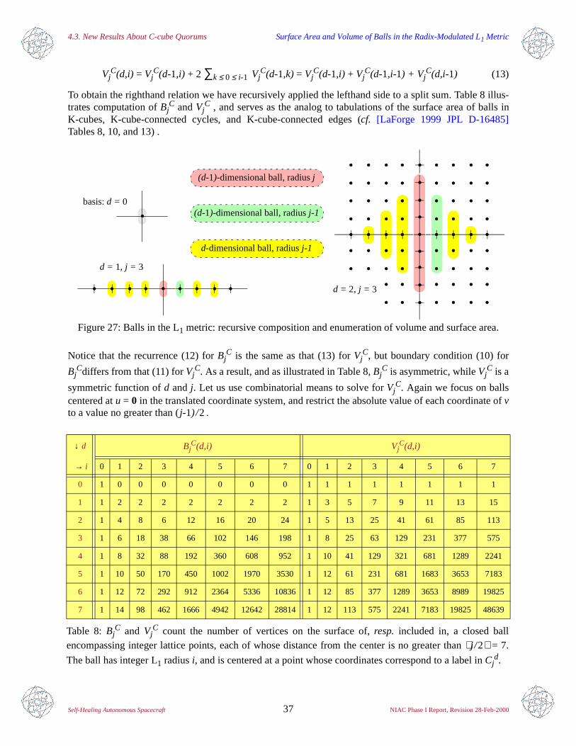
4.3. New Results About C-cube Quorums Surface Area and Volume of Balls in the Radix-Modulated L1 Metric
Self-Healing Autonomous Spacecraft 37 NIAC Phase I Report, Revision 28-Feb-2000
VjC(d,i) = Vj
C(d-1,i) + 2 ∑k ≤ 0 ≤ i-1 VjC(d-1,k) = Vj
C(d-1,i) + VjC(d-1,i-1) + Vj
C(d,i-1) (13)
To obtain the righthand relation we have recursively applied the lefthand side to a split sum. Table 8 illus-trates computation of Bj
C and VjC , and serves as the analog to tabulations of the surface area of balls in
K-cubes, K-cube-connected cycles, and K-cube-connected edges (cf. [LaForge 1999 JPL D-16485]Tables 8, 10, and 13) .
Notice that the recurrence (12) for BjC is the same as that (13) for Vj
C, but boundary condition (10) for
BjCdiffers from that (11) for Vj
C. As a result, and as illustrated in Table 8, BjC is asymmetric, while Vj
C is a
symmetric function of d and j. Let us use combinatorial means to solve for VjC. Again we focus on balls
centered at u = 0 in the translated coordinate system, and restrict the absolute value of each coordinate of vto a value no greater than (j-1) /2 .
Figure 27: Balls in the L1 metric: recursive composition and enumeration of volume and surface area.
↓ d BjC(d,i) Vj
C(d,i)
→ i 0 1 2 3 4 5 6 7 0 1 2 3 4 5 6 7
0 1 0 0 0 0 0 0 0 1 1 1 1 1 1 1 1
1 1 2 2 2 2 2 2 2 1 3 5 7 9 11 13 15
2 1 4 8 6 12 16 20 24 1 5 13 25 41 61 85 113
3 1 6 18 38 66 102 146 198 1 8 25 63 129 231 377 575
4 1 8 32 88 192 360 608 952 1 10 41 129 321 681 1289 2241
5 1 10 50 170 450 1002 1970 3530 1 12 61 231 681 1683 3653 7183
6 1 12 72 292 912 2364 5336 10836 1 12 85 377 1289 3653 8989 19825
7 1 14 98 462 1666 4942 12642 28814 1 12 113 575 2241 7183 19825 48639
Table 8: BjC and Vj
C count the number of vertices on the surface of, resp. included in, a closed ballencompassing integer lattice points, each of whose distance from the center is no greater than j / 2 = 7.
The ball has integer L1 radiusi, and is centered at a point whose coordinates correspond to a label in Cjd.
d = 2, j = 3
basis: d = 0
d = 1, j = 3
(d-1)-dimensional ball, radius j-1
(d-1)-dimensional ball, radius j
d-dimensional ball, radius j-1
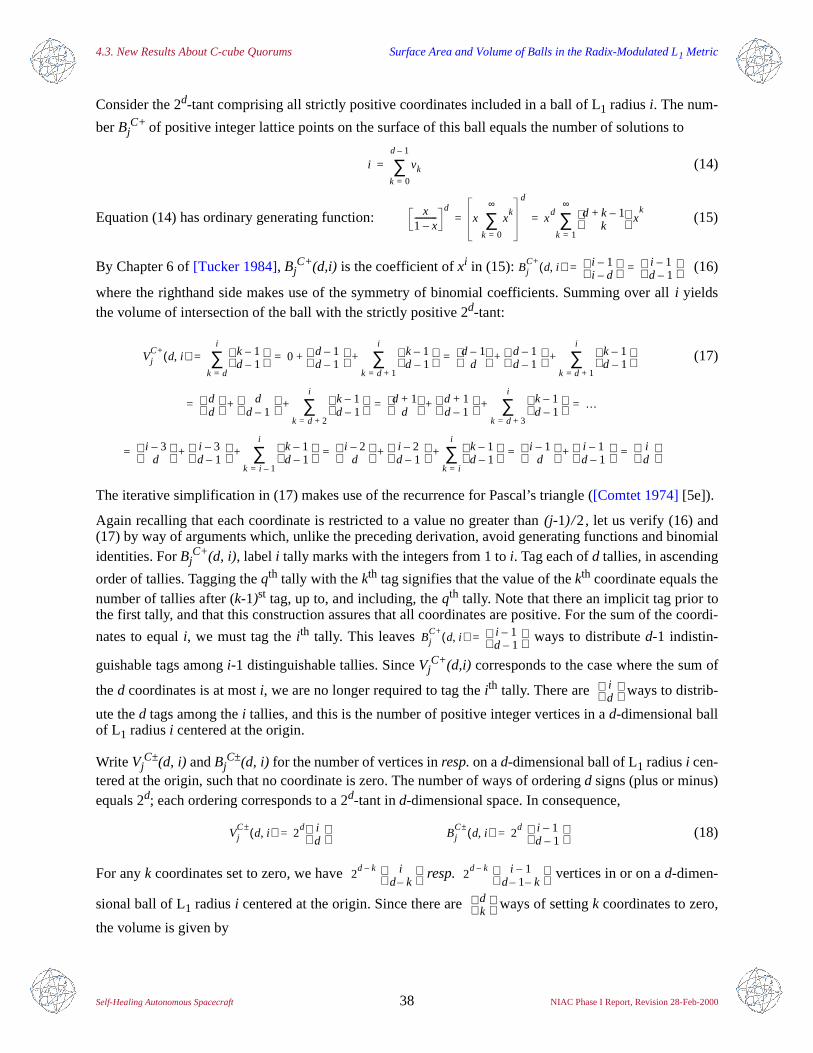
4.3. New Results About C-cube Quorums Surface Area and Volume of Balls in the Radix-Modulated L1 Metric
Self-Healing Autonomous Spacecraft 38 NIAC Phase I Report, Revision 28-Feb-2000
Consider the 2d-tant comprising all strictly positive coordinates included in a ball of L1 radius i. The num-
ber BjC+ of positive integer lattice points on the surface of this ball equals the number of solutions to
(14)
Equation (14) has ordinary generating function: (15)
By Chapter 6 of [Tucker 1984], BjC+(d,i) is the coefficient of xi in (15): (16)
where the righthand side makes use of the symmetry of binomial coefficients. Summing over all i yieldsthe volume of intersection of the ball with the strictly positive 2d-tant:
(17)
The iterative simplification in (17) makes use of the recurrence for Pascal’s triangle ([Comtet 1974] [5e]).
Again recalling that each coordinate is restricted to a value no greater than (j-1)/2, let us verify (16) and(17) by way of arguments which, unlike the preceding derivation, avoid generating functions and binomialidentities. For Bj
C+(d, i), label i tally marks with the integers from 1 to i. Tag each of d tallies, in ascending
order of tallies. Tagging the qth tally with the kth tag signifies that the value of the kth coordinate equals thenumber of tallies after (k-1)st tag, up to, and including, the qth tally. Note that there an implicit tag prior tothe first tally, and that this construction assures that all coordinates are positive. For the sum of the coordi-
nates to equal i, we must tag the ith tally. This leaves ways to distribute d-1 indistin-
guishable tags among i-1 distinguishable tallies. Since VjC+(d,i) corresponds to the case where the sum of
the d coordinates is at most i, we are no longer required to tag the ith tally. There are ways to distrib-
ute the d tags among the i tallies, and this is the number of positive integer vertices in a d-dimensional ballof L1 radius i centered at the origin.
Write VjC±(d, i) and Bj
C±(d, i) for the number of vertices in resp. on a d-dimensional ball of L1 radius i cen-tered at the origin, such that no coordinate is zero. The number of ways of ordering d signs (plus or minus)equals 2d; each ordering corresponds to a 2d-tant in d-dimensional space. In consequence,
(18)
For any k coordinates set to zero, we have resp. vertices in or on a d-dimen-
sional ball of L1 radius i centered at the origin. Since there are ways of setting k coordinates to zero,
the volume is given by
i vkk 0=
d 1–
∑=
x1 x–-----------
dx x
k
k 0=
∞
∑d
xd d k 1–+
k x
k
k 1=
∞
∑= =
BjC+
d i,( ) i 1–i d–
i 1–d 1–
= =
VjC+
d i,( ) k 1–d 1–
k d=
i
∑ 0 d 1–d 1–
k 1–d 1–
k d 1+=
i
∑+ + d 1–d
d 1–d 1–
k 1–d 1–
k d 1+=
i
∑+ +
dd
dd 1–
k 1–d 1–
k d 2+=
i
∑+ + d 1+d
d 1+d 1–
k 1–d 1–
k d 3+=
i
∑+ + …
i 3–d
i 3–d 1–
k 1–d 1–
k i 1–=
i
∑+ + i 2–d
i 2–d 1–
k 1–d 1–
k i=
i
∑+ + i 1–d
i 1–d 1–
+ id
= = =
= = =
= = = =
BjC+
d i,( ) i 1–d 1–
=
id
VjC±
d i,( ) 2d i
d = Bj
C±d i,( ) 2
d i 1–d 1–
=
2d k– i
d k– 2
d k– i 1–d 1 k––
dk
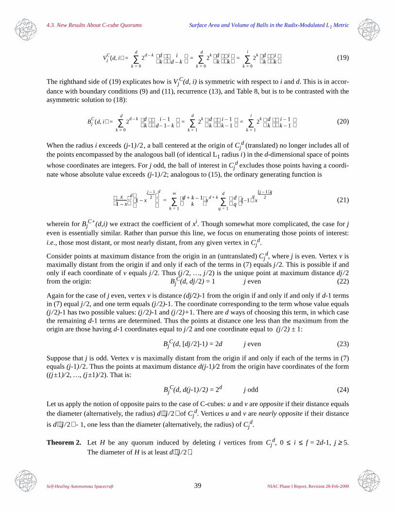
4.3. New Results About C-cube Quorums Surface Area and Volume of Balls in the Radix-Modulated L1 Metric
Self-Healing Autonomous Spacecraft 39 NIAC Phase I Report, Revision 28-Feb-2000
(19)
The righthand side of (19) explicates how is VjC(d, i) is symmetric with respect to i and d. This is in accor-
dance with boundary conditions (9) and (11), recurrence (13), and Table 8, but is to be contrasted with theasymmetric solution to (18):
(20)
When the radius i exceeds (j-1) /2, a ball centered at the origin of Cjd (translated) no longer includes all of
the points encompassed by the analogous ball (of identical L1 radius i ) in the d-dimensional space of points
whose coordinates are integers. For j odd, the ball of interest in Cjd excludes those points having a coordi-
nate whose absolute value exceeds (j-1)/2; analogous to (15), the ordinary generating function is
(21)
wherein for BjC+(d,i) we extract the coefficient of xi. Though somewhat more complicated, the case for j
even is essentially similar. Rather than pursue this line, we focus on enumerating those points of interest:i.e., those most distant, or most nearly distant, from any given vertex in Cj
d.
Consider points at maximum distance from the origin in an (untranslated) Cjd, where j is even. Vertex v is
maximally distant from the origin if and only if each of the terms in (7) equals j / 2. This is possible if andonly if each coordinate of v equals j / 2. Thus (j / 2, …, j/2) is the unique point at maximum distance dj/2from the origin: Bj
C(d, dj/2) = 1 j even (22)
Again for the case of j even, vertex v is distance (dj/2)-1 from the origin if and only if and only if d-1 termsin (7) equal j / 2, and one term equals (j /2)-1. The coordinate corresponding to the term whose value equals(j / 2)-1 has two possible values: (j / 2)-1 and (j / 2)+1. There are d ways of choosing this term, in which casethe remaining d-1 terms are determined. Thus the points at distance one less than the maximum from theorigin are those having d-1 coordinates equal to j / 2 and one coordinate equal to (j / 2) ± 1:
BjC(d, [dj/2]-1) = 2d j even (23)
Suppose that j is odd. Vertex v is maximally distant from the origin if and only if each of the terms in (7)equals (j-1)/2. Thus the points at maximum distance d(j-1)/2 from the origin have coordinates of the form((j ±1)/2, …, (j±1)/2). That is:
BjC(d, d(j-1)/2) = 2d j odd (24)
Let us apply the notion of opposite pairs to the case of C-cubes: u and v are opposite if their distance equalsthe diameter (alternatively, the radius) d⋅ j / 2 of Cj
d. Vertices u and v are nearly opposite if their distance
is d⋅ j / 2 - 1, one less than the diameter (alternatively, the radius) of Cjd.
Theorem 2. Let H be any quorum induced by deleting i vertices from Cjd, 0 ≤ i ≤ f = 2d-1, j ≥ 5.
The diameter of H is at least d⋅ j / 2 .
VjC
d i,( ) 2d k– d
k i
d k–
k 0=
d
∑ 2k d
k i
k
k 0=
d
∑ 2k d
k i
k
k 0=
i
∑= = =
BjC
d i,( ) 2d k– d
k i 1–
d 1 k––
k 0=
d
∑ 2k d
k i 1–
k 1–
k 1=
d
∑ 2k d
k i 1–
k 1–
k 1=
i
∑= = =
x1 x–-----------
d1 x
j 1–2
----------
–
d
d k 1–+k
xd k+ d
q 1–( )
qx
j 1–( )q2
------------------
q 1=
d
∑k 1=
∞
∑=
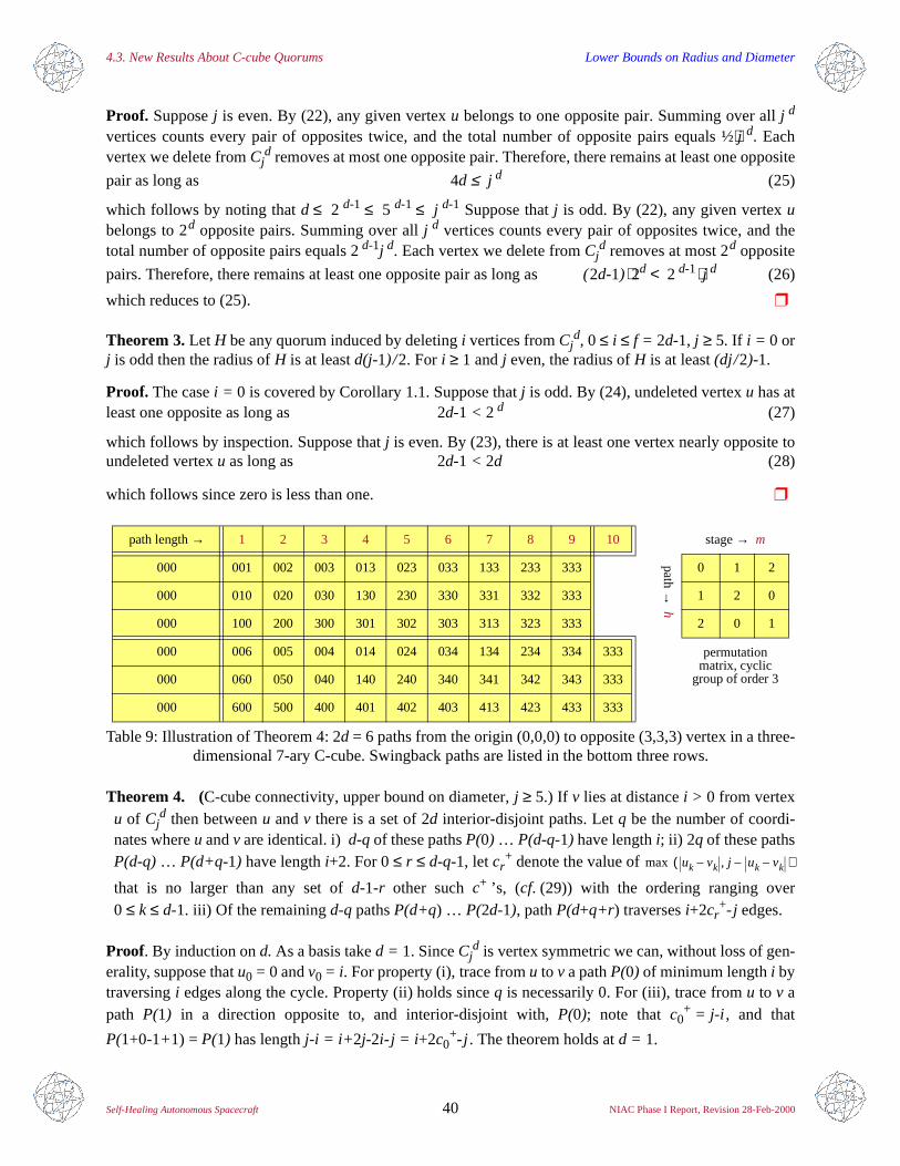
4.3. New Results About C-cube Quorums Lower Bounds on Radius and Diameter
Self-Healing Autonomous Spacecraft 40 NIAC Phase I Report, Revision 28-Feb-2000
Proof. Suppose j is even. By (22), any given vertex u belongs to one opposite pair. Summing over all j d
vertices counts every pair of opposites twice, and the total number of opposite pairs equals ½⋅j d. Eachvertex we delete from Cj
d removes at most one opposite pair. Therefore, there remains at least one opposite
pair as long as 4d ≤ j d (25)
which follows by noting that d ≤ 2 d-1 ≤ 5 d-1 ≤ j d-1 Suppose that j is odd. By (22), any given vertex ubelongs to 2d opposite pairs. Summing over all j d vertices counts every pair of opposites twice, and thetotal number of opposite pairs equals 2 d-1j d. Each vertex we delete from Cj
d removes at most 2d opposite
pairs. Therefore, there remains at least one opposite pair as long as (2d-1) ⋅2d < 2 d-1⋅ j d (26)
which reduces to (25).
Theorem 3. Let H be any quorum induced by deleting i vertices from Cjd, 0 ≤ i ≤ f = 2d-1, j ≥ 5. If i = 0 or
j is odd then the radius of H is at least d(j-1)/2. For i ≥ 1 and j even, the radius of H is at least (dj/2)-1.
Proof. The case i = 0 is covered by Corollary 1.1. Suppose that j is odd. By (24), undeleted vertex u has atleast one opposite as long as 2d-1 < 2 d (27)
which follows by inspection. Suppose that j is even. By (23), there is at least one vertex nearly opposite toundeleted vertex u as long as 2d-1 < 2d (28)
which follows since zero is less than one.
Theorem 4. (C-cube connectivity, upper bound on diameter, j ≥ 5.) If v lies at distance i > 0 from vertexu of Cj
d then between u and v there is a set of 2d interior-disjoint paths. Let q be the number of coordi-nates where u and v are identical. i) d-q of these paths P(0) … P(d-q-1) have length i; ii) 2q of these pathsP(d-q) … P(d+q-1) have length i+2. For 0≤ r ≤ d-q-1, let cr
+ denote the value of
that is no larger than any set of d-1-r other such c+ ’s, (cf. (29)) with the ordering ranging over0 ≤ k ≤ d-1. iii) Of the remaining d-q paths P(d+q) … P(2d-1), path P(d+q+r) traverses i+2cr
+- j edges.
Proof. By induction on d. As a basis take d = 1. Since Cjd is vertex symmetric we can, without loss of gen-
erality, suppose that u0 = 0 and v0 = i. For property (i), trace from u to v a path P(0) of minimum length i bytraversing i edges along the cycle. Property (ii) holds since q is necessarily 0. For (iii), trace from u to v apath P(1) in a direction opposite to, and interior-disjoint with, P(0); note that c0
+ = j-i , and that
P(1+0-1+1) = P(1) has length j-i = i+ 2j-2i- j = i +2c0+- j . The theorem holds at d = 1.
path length → 1 2 3 4 5 6 7 8 9 10 path → h
stage → m
000 001 002 003 013 023 033 133 233 333 0 1 2
000 010 020 030 130 230 330 331 332 333 1 2 0
000 100 200 300 301 302 303 313 323 333 2 0 1
000 006 005 004 014 024 034 134 234 334 333 permutation matrix, cyclic
group of order 3000 060 050 040 140 240 340 341 342 343 333
000 600 500 400 401 402 403 413 423 433 333
Table 9: Illustration of Theorem 4: 2d = 6 paths from the origin (0,0,0) to opposite (3,3,3) vertex in a three-dimensional 7-ary C-cube. Swingback paths are listed in the bottom three rows.
max uk vk– j uk vk––,( )
4.3. New Results About C-cube Quorums Constructive Upper Bounds on Diameter
Self-Healing Autonomous Spacecraft 41 NIAC Phase I Report, Revision 28-Feb-2000
Assume that the theorem holds in 0, … (d-1) dimensions, and regard arbitrary vertices u and v in Cjd,
d > 1, j ≥ 4. Suppose that q = 0; i.e., the coordinates of u and v differ in all d dimensions.
i) For the 0th coordinate, trace a shortest path P ′(0), of length min(|u0-v0|, j-|u0-v0| ), from u to
(ud-1, … , v0). By induction, the Cjd-1 prescribed by setting the 0th coordinate to v0 contains a path P ″(0)
from (ud-1, … , v0) to v, and this path traverses i-min(|u0-v0|, j-|u0-v0| ) edges. Catenating P ′(0) with P ″(0)gives an i-edge path P(0) from u to v. For h = 1, …d-1, iterate this process to synthesize path P(h): at thestart of the hth iteration rotate each coordinate value by adding it to h, and converting the sum to its princi-pal value mod d. As illustrated by the righthand side of Table 9, this completes a symmetric permutationmatrix for the cyclic group of order d [Artin 1975] (VII:1.4). At h = 2, for example, coordinates along thepath change in the order 2, …,d-1, 0, 1. With respect to any vertex along a path, define the stage to be thenumber m of different coordinates that have changed; q = 0 implies 0≤ m ≤ d-1. Entry (h, m) of the permu-tation matrix equals (h+m) mod d. Consider any two paths P(h1) and P(h2), for any stage m < d-1. Sinceentries 0 through m of any row map to successive elements of the cyclic group of order d, at least one of thevalues in columns 0 through m of row h1 (resp. h2) must not be in columns 0 through m of row h2 (resp.h2). But this means that, through stage m, the set of coordinates of P(h1) that are unchanged from theiroriginal values in u differ from the coordinates of P(h2) that are unchanged from their original values in u.Thus, the only possible intersection of P(h1) and P(h2) is at stage d-1. But this is also impossible: the
(h1 + d-1 modd-1)th coordinate in P(h1) increments, in a monotone fashion modulo d-1, toward the coor-dinate value of v in that dimension, while the remaining paths have already attained the coordinate value ofv in that dimension. Therefore, any path so constructed is interior-disjoint with any other.
iii) Continuing the case for q = 0, construct an additional d paths by substituting a swingback at the 0th
stage of the preceding procedure. For stages 0 through d-1, that is, begin by tracing a path P ′(d-1+h) oflength max( |uh-vh|, j-|uh-vh| ) from u to (ud-1, … , vh±1 mod j, … , u0); if max(|uh-vh|, j-|uh-vh|) = j-|uh-vh|then the zeroth stage path stops at vh +1 mod j; otherwise it stops at vh -1 mod j.
This construction results in a swingback path P(h) passing through a neighbor of v, with the hth coordinateequal to vh±1. As illustrated by the bottom three rows of Table 9, the final step in the path traverses an edgeto v. Note that the total length of P(h) is i+j- 2|uh-vh| if min( |uh-vh|, j-|uh-vh|) = |uh-vh|; otherwise,min(|uh-vh|, j-|uh-vh|) = j-|uh-vh| and the path length is i-j+ 2|uh-vh|. In any case, sorting the swingback
paths by their lengths yields a set of d-q = d-0 = d paths P(d) … P(2d-1), with P(d+r) traversing i+2cr+- j
edges, and 0≤ r ≤ d-q-1 = d-1.
By an argument similar to that pertaining to paths without swingback, any path with swingback intersectsno other path (with or without swingback), at least up to the next-to-last edge in the path. As remarked pre-viously, the next-to-last edge advances to a unique neighbor of v (i.e., one which has not been traversed byany other path, with or without swingback). For q = 0, that is, any two paths constructed in steps (i) or (iii)are interior-disjoint.
Now suppose that the integer q is positive. With u as source and v as destination, inductively apply the pre-ceding procedure for q = 0 to the d-q coordinates not shared by u and v. i) The Cj
d-1 prescribed by the qcoordinates whose values are the same in u and v contains 2(d-q) pairwise interior-disjoint u-v paths, d-q ofwhich traverse i edges.
ii) Construct 2q bypass paths as follows. If k is the index of a coordinate such that uk = vk, then traverse to
a neighbor of u by crossing one edge in the kth dimension; i.e., by incrementing or decrementing uk. From
this neighbor construct a path to the neighbor of v obtained by incrementing resp. decrementing the kth
coordinate of v. From u’s neighbor to v’s neighbor, a single path of length i is guaranteed by applying theprocedure for q = 0 to the d-q coordinates not shared by u and v. Traversing from v’s neighbor to v com-
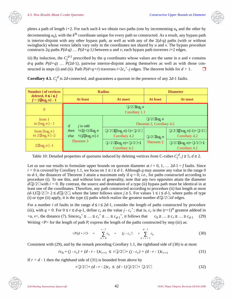
4.3. New Results About C-cube Quorums Constructive Upper Bounds on Diameter
Self-Healing Autonomous Spacecraft 42 NIAC Phase I Report, Revision 28-Feb-2000
pletes a path of length i+ 2. For each such k we obtain two paths (one by incrementing uk and the other by
decrementing uk), with the kth coordinate unique for every path so constructed. As a result, any bypass pathis interior-disjoint with any other bypass path, as well as with any of the 2(d-q) paths (with or withoutswingback) whose vertex labels vary only in the coordinates not shared by u and v. The bypass procedureconstructs 2q paths P(d-q) … P(d+q-1) between u and v; each bypass path traverses i+2 edges.
iii) By induction, the Cjd-1 prescribed by the q coordinates whose values are the same in u and v contains
d-q paths P(d+q) … P(2d-1), pairwise interior-disjoint among themselves as well as with those con-structed in steps (i) and (ii). Path P(d+q+r) traverses i+2cr
+- j edges. The theorem holds for d > 1.
Corollary 4.1. Cjd is 2d-connected, and guarantees a quorum in the presence of any 2d-1 faults.
Let us use our results to formulate upper bounds on quorum diameter at i = 0, 1, … 2d-1 = f faults. Sincei = 0 is covered by Corollary 1.1, we focus on 1≤ i ≤ d-1. Although q may assume any value in the range 0to d-1, the distances of Theorem 3 attain a maximum only if q = 0; i.e., for paths constructed according toprocedure (i). To see this, and without loss of generality, note that any two opposites attain the diameterd⋅ j / 2 with i = 0. By contrast, the source and destination of a type (ii) bypass path must be identical in atleast one of the coordinates. Therefore, any path constructed according to procedure (ii) has length at most(d-1)⋅ j / 2 + 2 ≤ d⋅ j / 2 , where the latter follows since j ≥ 5. For values 1≤ i ≤ d-1, where paths of type(i) or type (ii) apply, it is the type (i) paths which realize the greatest number d⋅ j / 2 of edges.
For a number i of faults in the range d ≤ i ≤ 2d-1, consider the length of paths constructed by procedure(iii), with q = 0. For 0≤ r ≤ d-q-1, define cr as the value j - cr
+; that is, cr is the (r+1)st greatest addend in
<u, v>, the distance (7). Sincec0+ ≤ … ≤ cr
+ ≤ … ≤ cd-1+, it follows that c0 ≥ … ≥ cr ≥ … ≥ cd-1 (29)
Writing <P> for the length of path P, express the length of the paths constructed by step (iii) as:
(30)
Consistent with (29), and by the remark preceding Corollary 1.1, the righthand side of (30) is at most
rc0 + ( j - cr) + (d - r - 1)cr+ 1 ≤ r j / 2 + ( j - cr ) + (d - r - 1)cr+ 1 (31)
If r < d - 1 then the righthand side of (31) is bounded from above by
r j / 2 + (d - r - 2)cr ≤ (d - 1) j /2 + j /2 (32)
Number i of vertices deleted, 0≤≤≤≤ i ≤≤≤≤ ff = 2⋅⋅⋅⋅[logj n] - 1
Radius Diameter
At least At most At least At most
0 j / 2⋅logj n
Corollary 1.1
from 1to [logj n ] - 1
if j is oddthen ½⋅( j-1)⋅logj n
else ½⋅j ⋅[logj n]-1 Theorem 3
j / 2⋅logj nTheorem 2, Corollary 4.2
from [logj n ]to 2⋅[logj n ] -2
j / 2⋅([logj n]-1)+ j / 2 Corollary 4.2 j / 2⋅logj n
Theorem 2
j / 2⋅([logj n]-1)+ j / 2 Corollary 4.2
2⋅[logj n ] -1 j / 2⋅(logj n)+ j / 2−1
Corollary 4.2 j / 2⋅(logj n)+ j / 2−1
Corollary 4.2
Table 10: Detailed properties of quorums induced by deleting vertices from C-cubes Cjd, j ≥ 5, d ≥ 2.
<P d r+( )> ckk 0=
r 1–
∑ j cr–( ) ckk r 1+=
d 1–
∑+ +=
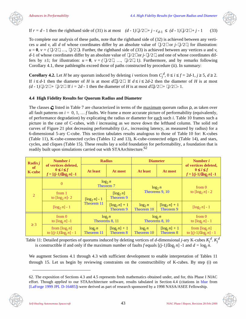
Advances in Performability 4.4. High Fidelity Results for Quorum Radius and Diameter
Self-Healing Autonomous Spacecraft 43 NIAC Phase I Report, Revision 28-Feb-2000
If r = d - 1 then the righthand side of (31) is at most(d - 1) j / 2 + j - cd-1 ≤ (d - 1) j / 2 + j - 1 (33)
To complete our analysis of these paths, note that the righthand side of (32) is achieved between any verti-ces u and v, all d of whose coordinates differ by an absolute value of j / 2 or j- j / 2 ; for illustration:u = 0, v = ( j / 2 , …, j / 2). Further, the righthand side of (33) is achieved between any vertices u and v,d-1 of whose coordinates differ by an absolute value of j / 2 or j- j / 2 , and one of whose coordinates dif-fers by ±1; for illustration: u = 0, v = ( j / 2 , …, j / 2 , 1). Furthermore, and by remarks followingCorollary 4.1, these pathlengths exceed those of paths constructed by procedure (ii). In summary:
Corollary 4.2. Let H be any quorum induced by deleting i vertices from Cjd, 0 ≤ i ≤ f = 2d-1, j ≥ 5, d ≥ 2.
If i ≤ d-1 then the diameter of H is at most d⋅ j / 2 . If d ≤ i ≤ 2d-2 then the diameter of H is at most(d - 1) j / 2 + j / 2. If i = 2d - 1 then the diameter of H is at most d⋅ j / 2 + j / 2 - 1.
4.4 High Fidelity Results for Quorum Radius and Diameter
The classes * listed in Table 7 are characterized in terms of the maximum quorum radius ρ, as taken overall fault patterns on i = 0, 1, … f faults. We frame a more accurate picture of performability (equivalently,of performance degradation) by explicating the radius or diameter for each such i. Table 10 frames such apicture in the case of C-cubes, with i increasing as we move down the lefthand column. The solid redcurves of Figure 21 plot decreasing performability (i.e., increasing latency, as measured by radius) for a6-dimensional 5-ary C-cube. This section tabulates results analogous to those of Table 10 for: K-cubes(Table 11), K-cube-connected cycles (Tables 12 and 13), K-cube-connected edges (Table 14), and stars,cycles, and cliques (Table 15). These results lay a solid foundation for performability, a foundation that isreadily built upon simulations carried out with STAArchitecture.62
We augment Sections 4.1 through 4.3 with sufficient development to enable interpretation of Tables 11through 15. Let us begin by reviewing constraints on the constructibility of K-cubes. By step (i) on
Radix j of
K-cube
Number i of vertices deleted,
0 ≤≤≤≤ i ≤≤≤≤ ff = [(j-1)⋅⋅⋅⋅logj n] -1
Radius Diameter Number i of vertices deleted,
0 ≤≤≤≤ i ≤≤≤≤ ff = [(j-1)⋅⋅⋅⋅logj n] -1
At least At most At least At most
2
0 log2 nTheorem 7 log2 n
Theorems 9, 10from 0
to [log2 n] - 2from 1to [log2 n]- 2 [log2 n] - 1
Theorem 11
[log2 n]Theorem 9
[log2 n] - 1 [log2 n] + 1Theorem 9
log2 nTheorem 10
[log2 n] + 1Theorem 9 [log2 n] - 1
≥ 3
from 0to [logj n] -1
logj nTheorems 8, 11
logj nTheorems 8, 10
from 0to [logj n] - 1
from [logj n]to [(j-1)⋅logj n] - 1
logj nTheorem 11
[logj n] + 1Theorem 8
logj nTheorem 10
[logj n] + 1Theorem 8
from [logj n]to [(j-1)⋅logj n] - 1
Table 11: Detailed properties of quorums induced by deleting vertices of d-dimensional j-ary K-cubes Kjd. Kj
d is constructible if and only if the maximum number of faults f equals [(j-1)⋅logj n] -1 and d = logj n.
62. The exposition of Sections 4.3 and 4.5 represents fresh mathematics obtained under, and for, this Phase I NIACeffort. Though applied to our STAArchitecture software, results tabulated in Section 4.4 (citations in blue from[LaForge 1999 JPL D-16485]) were derived as part of research sponsored by a 1998 NASA/ASEE Fellowship.
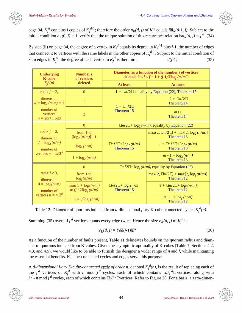
High-Fidelity Results for K-cubes 4.4. Constructibility, Quorum Radius and Diameter
Self-Healing Autonomous Spacecraft 44 NIAC Phase I Report, Revision 28-Feb-2000
page 34, Kjd contains j copies of Kj
d-1; therefore the order nK(d, j) of Kjd equals j⋅nK(d-1, j). Subject to the
initial condition nK(0, j) = 1, verify that the unique solution of this recurrence relation isnK(d, j) = j d (34)
By step (ii) on page 34, the degree of a vertex in Kjd equals its degree in Kj
d-1 plus j-1, the number of edges
that connect it to vertices with the same labels in the other copies of Kjd-1. Subject to the initial condition of
zero edges in Kj0, the degree of each vertex in Kj
d is therefore d(j-1) (35)
Summing (35) over all j d vertices counts every edge twice. Hence the size eK(d, j) of Kjd is
eK(d, j) = ½⋅d(j-1)⋅j d (36)
As a function of the number of faults present, Table 11 delineates bounds on the quorum radius and diam-eter of quorums induced from K-cubes. Given the asymptotic optimality of K-cubes (Table 7, Sections 4.2,4.3, and 4.5), we would like to be able to furnish the designer a wider range of n and f, while maintainingthe essential benefits. K-cube-connected cycles and edges serve this purpose.
A d-dimensional j-ary K-cube-connected cycle of order n, denoted Kjd(n), is the result of replacing each of
the j d vertices of Kjd with n mod j d cycles, each of which contains n/j d vertices, along with
j d - n mod j d cycles, each of which contains n/j d vertices. Refer to Figure 28. For a basis, a zero-dimen-
UnderlyingK-cubeKj
d(n)
Number i of vertices
deleted
Diameter, as a function of the number i of verticesdeleted, 0≤ i ≤ f = 1 + (j-1)⋅logj (n/m)
At least At most
radix j = 2,
dimensiond = log2 (n/m) = 1
number ofvertices
n = 2m+1 odd
0 1 + m/2 , equality by Equation (22), Theorem 15
11 + m/2
Theorem 15
2 + m/2Theorem 14
2m+1
Theorem 14
radix j = 2,
dimensiond = log2 (n/m)
number ofvertices n = m⋅2d
0 m/2 + log2 (n/m), equality by Equation (22)
from 1 to[log2 (n/m)] - 1
m/2 + log2 (n/m)Theorem 15
max(2, m/2 ) + max[2, log2 (n/m)]Theorem 13
log2 (n/m) 1 + m/2 + log2 (n/m)Theorem 13
1 + log2 (n/m)m -1 + log2 (n/m)
Theorem 13
radix j ≥ 3,
dimensiond = logj (n/m)
number ofvertices n = m⋅j d
0 m/2 + logj (n/m), equality by Equation (22)
from 1 tologj (n/m)
m/2 + logj (n/m)Theorem 15
max(2, m/2 ) + max[2, logj (n/m)]Theorem 12
from 1+ logj (n/m)to (j-1)⋅logj (n/m)
1 + m/2 + logj (n/m)Theorem 12
1 + (j- 1)⋅logj (n/m)m - 1 + logj (n/m)
Theorem 12
Table 12: Diameter of quorums induced from d-dimensional j-ary K-cube-connected cycles Kjd(n).
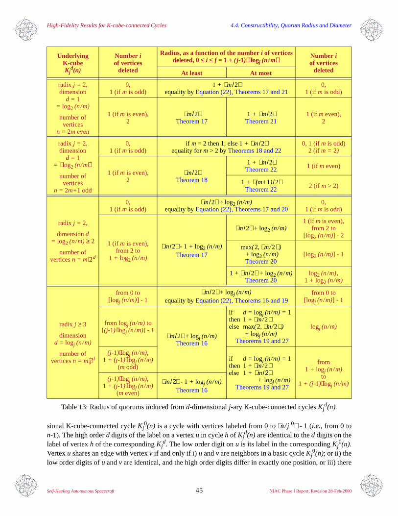
High-Fidelity Results for K-cube-connected Cycles 4.4. Constructibility, Quorum Radius and Diameter
Self-Healing Autonomous Spacecraft 45 NIAC Phase I Report, Revision 28-Feb-2000
sional K-cube-connected cycle Kj0(n) is a cycle with vertices labeled from 0 to n/j 0 - 1 (i.e., from 0 to
n-1). The high order d digits of the label on a vertex u in cycle h of Kjd(n) are identical to the d digits on the
label of vertex h of the corresponding Kjd. The low order digit on u is its label in the corresponding Kj
0(n).Vertex u shares an edge with vertex v if and only if i)u and v are neighbors in a basic cycle Kj
0(n); or ii) thelow order digits of u and v are identical, and the high order digits differ in exactly one position, or iii) there
UnderlyingK-cubeKj
d(n)
Number i of vertices
deleted
Radius, as a function of the number i of verticesdeleted, 0≤ i ≤ f = 1 + (j-1)⋅logj (n/m)
Number i of vertices
deletedAt least At most
radix j = 2,dimension
d = 1= log2 (n/m)
number ofvertices
n = 2m even
0,1 (if m is odd)
1 + m/2equality by Equation (22), Theorems 17 and 21
0,1 (if m is odd)
1 (if m is even),2
m/2Theorem 17
1 + m/2Theorem 21
1 (if m even),2
radix j = 2,dimension
d = 1= log2 (n/m)
number ofvertices
n = 2m+1 odd
0,1 (if m is odd)
if m = 2 then 1; else 1+ m/2equality for m > 2 by Theorems 18 and 22
0, 1 (if m is odd)2 (if m = 2)
1 (if m is even),2
m/2Theorem 18
1 + m/2Theorem 22 1 (if m even)
1 + (m+1)/2Theorem 22 2 (if m > 2)
radix j = 2,
dimension d= log2 (n/m)≥ 2
number ofvertices n = m⋅2d
0,1 (if m is odd)
m/2 + log2 (n/m)equality by Equation (22), Theorems 17 and 20
0,1 (if m is odd)
1 (if m is even),from 2 to
1 + log2 (n/m)
m/2 - 1 + log2 (n/m)Theorem 17
m/2 + log2 (n/m)1 (if m is even),
from 2 to[log2 (n/m)] - 2
max(2, m/2 )+ log2 (n/m)Theorem 20
[log2 (n/m)] - 1
1 + m/2 + log2 (n/m)Theorem 20
log2 (n/m),1 + log2 (n/m)
radix j ≥ 3
dimensiond = logj (n/m)
number ofvertices n = m⋅j d
from 0 to[logj (n/m)] - 1
m/2 + logj (n/m)equality by Equation (22), Theorems 16 and 19
from 0 to[logj (n/m)] - 1
from logj (n/m) to[(j-1)⋅logj (n/m)] - 1
m/2 + logj (n/m)Theorem 16
if d = logj (n/m) = 1then 1+ m/2else max(2, m/2 )
+ logj (n/m) Theorems 19 and 27
logj (n/m)
(j-1)⋅logj (n/m),1 + (j- 1)⋅logj (n/m)
(m odd)if d = logj (n/m) = 1then 1+ m/2else 1+ m/2
+ logj (n/m) Theorems 19 and 27
from1 + logj (n/m)
to1 + (j- 1)⋅logj (n/m)
(j-1)⋅logj (n/m),1 + (j- 1)⋅logj (n/m)
(m even)
m/2 - 1 + logj (n/m)Theorem 16
Table 13: Radius of quorums induced from d-dimensional j-ary K-cube-connected cycles Kjd(n).
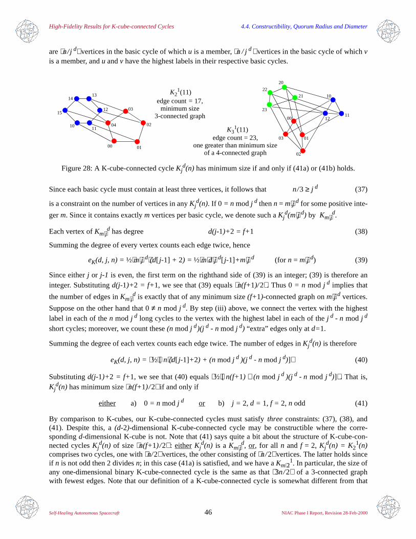
High-Fidelity Results for K-cube-connected Cycles 4.4. Constructibility, Quorum Radius and Diameter
Self-Healing Autonomous Spacecraft 46 NIAC Phase I Report, Revision 28-Feb-2000
are n/j d vertices in the basic cycle of which u is a member, n / j d vertices in the basic cycle of which vis a member, and u and v have the highest labels in their respective basic cycles.
Since each basic cycle must contain at least three vertices, it follows that n/3 ≥ j d (37)
is a constraint on the number of vertices in any Kjd(n). If 0 = n mod j d then n = m⋅j d for some positive inte-
ger m. Since it contains exactly m vertices per basic cycle, we denote such a Kjd(m⋅j d) by Km⋅j
d.
Each vertex of Km⋅jd has degree d(j-1)+2 = f+1 (38)
Summing the degree of every vertex counts each edge twice, hence
eK(d, j, n) = ½⋅m⋅j d⋅(d[ j-1] + 2) = ½⋅m⋅d⋅j d[ j-1]+m⋅j d (for n = m⋅j d) (39)
Since either j or j-1 is even, the first term on the righthand side of (39) is an integer; (39) is therefore aninteger. Substituting d(j-1)+2 = f+1, we see that (39) equals n(f+1)/2. Thus 0 = n mod j d implies that
the number of edges in Km⋅jd is exactly that of any minimum size (f+1)-connected graph on m⋅j d vertices.
Suppose on the other hand that 0 ≠ n mod j d. By step (iii) above, we connect the vertex with the highestlabel in each of the n mod j d long cycles to the vertex with the highest label in each of the j d - n mod j d
short cycles; moreover, we count these (n mod j d)(j d - n mod j d) “extra” edges only at d=1.
Summing the degree of each vertex counts each edge twice. The number of edges in Kjd(n) is therefore
eK(d, j, n) = ½⋅[ n⋅(d[ j-1]+2) + (n mod j d )(j d - n mod j d)] (40)
Substituting d(j-1)+2 = f+1, we see that (40) equals ½⋅[ n(f+1) + (n mod j d )(j d - n mod j d)] . That is,Kj
d(n) has minimum size n(f+1)/2 if and only if
either a) 0 = n mod j d or b) j = 2, d = 1, f = 2, n odd (41)
By comparison to K-cubes, our K-cube-connected cycles must satisfy three constraints: (37), (38), and(41). Despite this, a (d-2)-dimensional K-cube-connected cycle may be constructible where the corre-sponding d-dimensional K-cube is not. Note that (41) says quite a bit about the structure of K-cube-con-nected cycles Kj
d(n) of size n(f+1) /2 : either Kjd(n) is a Km⋅j
d, or, for all n and f = 2, Kjd(n) = K2
1(n)comprises two cycles, one with n/2 vertices, the other consisting ofn/2 vertices. The latter holds sinceif n is not odd then 2 divides n; in this case (41a) is satisfied, and we have a Km⋅2
1. In particular, the size ofany one-dimensional binary K-cube-connected cycle is the same as that 3n/2 of a 3-connected graphwith fewest edges. Note that our definition of a K-cube-connected cycle is somewhat different from that
Figure 28: A K-cube-connected cycle Kjd(n) has minimum size if and only if (41a) or (41b) holds.
01
00
03
12
10
11
22
20
21
K31(11)
K21(11)
02
edge count = 17,minimum size
10
0315
01
1314
11
00
12
0204
23
edge count = 23,one greater than minimum size
3-connected graph
of a 4-connected graph
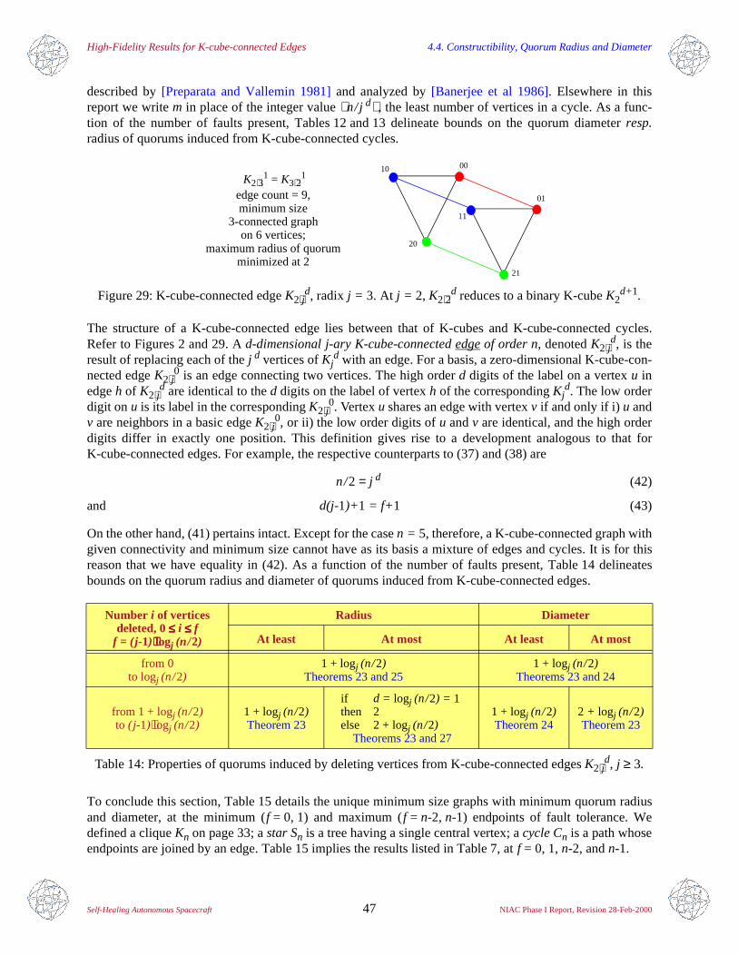
High-Fidelity Results for K-cube-connected Edges 4.4. Constructibility, Quorum Radius and Diameter
Self-Healing Autonomous Spacecraft 47 NIAC Phase I Report, Revision 28-Feb-2000
described by [Preparata and Vallemin 1981] and analyzed by [Banerjee et al 1986]. Elsewhere in thisreport we write m in place of the integer value n/j d , the least number of vertices in a cycle. As a func-tion of the number of faults present, Tables 12 and 13 delineate bounds on the quorum diameter resp.radius of quorums induced from K-cube-connected cycles.
The structure of a K-cube-connected edge lies between that of K-cubes and K-cube-connected cycles.Refer to Figures 2 and 29. A d-dimensional j-ary K-cube-connected edge of order n, denoted K2⋅j
d, is theresult of replacing each of the j d vertices of Kj
d with an edge. For a basis, a zero-dimensional K-cube-con-nected edge K2⋅j
0 is an edge connecting two vertices. The high order d digits of the label on a vertex u inedge h of K2⋅j
d are identical to the d digits on the label of vertex h of the corresponding Kjd. The low order
digit on u is its label in the corresponding K2⋅j0. Vertex u shares an edge with vertex v if and only if i)u and
v are neighbors in a basic edge K2⋅j0, or ii) the low order digits of u and v are identical, and the high order
digits differ in exactly one position. This definition gives rise to a development analogous to that forK-cube-connected edges. For example, the respective counterparts to (37) and (38) are
n/2 = j d (42)
and d(j-1)+1 = f+1 (43)
On the other hand, (41) pertains intact. Except for the case n = 5, therefore, a K-cube-connected graph withgiven connectivity and minimum size cannot have as its basis a mixture of edges and cycles. It is for thisreason that we have equality in (42). As a function of the number of faults present, Table 14 delineatesbounds on the quorum radius and diameter of quorums induced from K-cube-connected edges.
To conclude this section, Table 15 details the unique minimum size graphs with minimum quorum radiusand diameter, at the minimum (f = 0, 1) and maximum (f = n-2, n-1) endpoints of fault tolerance. Wedefined a clique Kn on page 33; a star Sn is a tree having a single central vertex; a cycle Cn is a path whoseendpoints are joined by an edge. Table 15 implies the results listed in Table 7, at f = 0, 1,n-2, andn-1.
Figure 29: K-cube-connected edge K2⋅jd, radix j = 3. At j = 2, K2⋅2
d reduces to a binary K-cube K2d+1.
Number i of vertices deleted, 0≤≤≤≤ i ≤≤≤≤ f
f = (j-1)⋅⋅⋅⋅logj (n/2)
Radius Diameter
At least At most At least At most
from 0to logj (n/2)
1 + logj (n/2)Theorems 23 and 25
1 + logj (n/2)Theorems 23 and 24
from 1 + logj (n/2)to (j-1)⋅logj (n/2)
1 + logj (n/2)Theorem 23
if d = logj (n/2) = 1then 2else 2 + logj (n/2) Theorems 23 and 27
1 + logj (n/2)Theorem 24
2 + logj (n/2)Theorem 23
Table 14: Properties of quorums induced by deleting vertices from K-cube-connected edges K2⋅jd, j ≥ 3.
K2⋅31 = K3⋅2
1
edge count = 9,minimum size
10 00
20
3-connected graph 11
01
21
on 6 vertices;maximum radius of quorum
minimized at 2
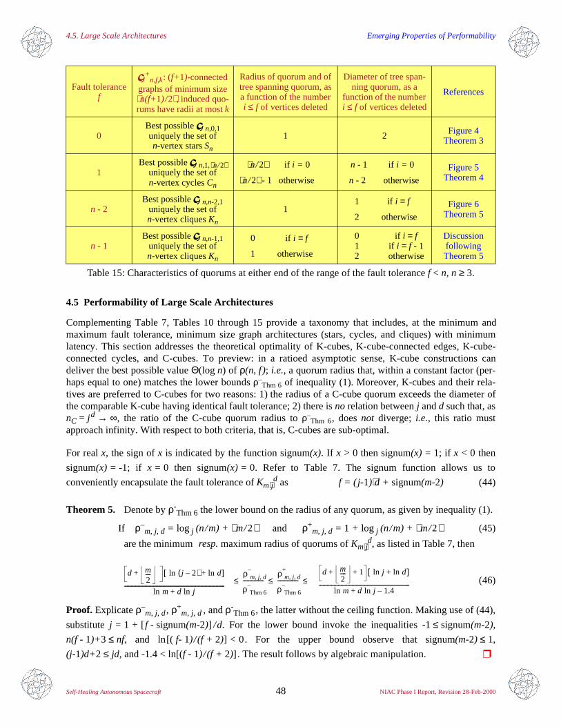
4.5. Large Scale Architectures Emerging Properties of Performability
Self-Healing Autonomous Spacecraft 48 NIAC Phase I Report, Revision 28-Feb-2000
4.5 Performability of Large Scale Architectures
Complementing Table 7, Tables 10 through 15 provide a taxonomy that includes, at the minimum andmaximum fault tolerance, minimum size graph architectures (stars, cycles, and cliques) with minimumlatency. This section addresses the theoretical optimality of K-cubes, K-cube-connected edges, K-cube-connected cycles, and C-cubes. To preview: in a ratioed asymptotic sense, K-cube constructions candeliver the best possible value Θ(log n) of ρ(n, f); i.e., a quorum radius that, within a constant factor (per-haps equal to one) matches the lower bounds ρ–
Thm 6 of inequality (1). Moreover, K-cubes and their rela-tives are preferred to C-cubes for two reasons: 1) the radius of a C-cube quorum exceeds the diameter ofthe comparable K-cube having identical fault tolerance; 2) there is no relation between j and d such that, asnC = j d → ∞, the ratio of the C-cube quorum radius to ρ–
Thm 6, does not diverge; i.e., this ratio mustapproach infinity. With respect to both criteria, that is, C-cubes are sub-optimal.
For real x, the sign of x is indicated by the function signum(x). If x > 0 then signum(x) = 1; if x < 0 then
signum(x) = -1; if x = 0 then signum(x) = 0. Refer to Table 7. The signum function allows us to
conveniently encapsulate the fault tolerance of Km⋅jd as f = ( j-1)⋅d + signum(m-2) (44)
Theorem 5. Denote by ρ-Thm 6 the lower bound on the radius of any quorum, as given by inequality (1).
If ρ–m, j, d= log j (n/m) + m/2 and ρ+
m, j, d= 1 + log j (n/m) + m/2 (45)
are the minimum resp. maximum radius of quorums of Km⋅jd, as listed in Table 7, then
(46)
Proof. Explicate ρ–m, j, d, ρ+
m, j, d, and ρ-Thm 6, the latter without the ceiling function. Making use of (44),
substitute j = 1 + [ f - signum(m-2)] /d. For the lower bound invoke the inequalities -1≤ signum(m-2),
n(f - 1)+3 ≤ nf, and ln[(f- 1)/(f + 2)] < 0. For the upper bound observe that signum(m-2) ≤ 1,
(j-1)d+2 ≤ jd, and -1.4 < ln[(f - 1)/(f + 2)] . The result follows by algebraic manipulation.
Fault tolerancef
*+n,f,k: (f+1)-connected
graphs of minimum size n(f+1)/2, induced quo-rums have radii at most k
Radius of quorum and of tree spanning quorum, as a function of the number i ≤ f of vertices deleted
Diameter of tree span-ning quorum, as a
function of the number i ≤ f of vertices deleted
References
0Best possible *
n,0,1uniquely the set ofn-vertex stars Sn
1 2 Figure 4Theorem 3
1Best possible *
n,1,n/2uniquely the set ofn-vertex cycles Cn
n/2 if i = 0
n/2 - 1 otherwise
n - 1 if i = 0
n - 2 otherwise
Figure 5Theorem 4
n - 2Best possible *
n,n-2,1 uniquely the set ofn-vertex cliques Kn
11 if i = f
2 otherwise
Figure 6Theorem 5
n - 1Best possible *
n,n-1,1 uniquely the set ofn-vertex cliques Kn
0 if i = f
1 otherwise
0 if i = f1 if i = f - 12 otherwise
DiscussionfollowingTheorem 5
Table 15: Characteristics of quorums at either end of the range of the fault tolerance f < n, n≥ 3.
d m2----+ ln j 2–( ) ln d+[ ]
ln m d+ ln j-------------------------------------------------------------------------
ρ m j d, ,–
ρ Thm 6–
---------------ρ m j d, ,
+
ρ Thm 6–
---------------d m
2---- 1+ + ln j ln d+[ ]
ln m d+ ln j 1.4–------------------------------------------------------------------≤ ≤ ≤
4.5. Large Scale Architectures Members of the K-cube Family Converge to the Moore Bound
Self-Healing Autonomous Spacecraft 49 NIAC Phase I Report, Revision 28-Feb-2000
It is interesting to note that, in the large, the fault tolerance (44) of Km⋅jd is dominated by j and d, and grows
in a fashion that is independent of m. By contrast, the radius of Km⋅jd is dominated by m and d, and is inde-
pendent of j. Our conclusions about the optimality of the quorum radius of Km⋅jd depend on how m, j, and d
tend to infinity. If the left and right sides of (46) tend to some limit λ then, in the large, ρ–m, j, d, ρ+
m, j, d,
and ρ–Thm 6 are within a factor λ of ρ(m⋅j d, (j-1)⋅d + signum[m-2] ), the minimum value (over all graphs)
of the maximum quorum radius. Abbreviating the latter quantity as ρ m, j, d, we obtain the following result.
Corollary 5.1. For all nK = m⋅j d ≥ k, if q and r are least upper bounds
such that and , then .
Under the conditions of Corollary 5.1, that is, the maximum quorum radius of Km⋅jd approaches a value
that is within a factor 1+ q + qr + r of the minimum. Several special cases of Corollary 5.1 are of particu-lar interest: a) d ∈ o(j); b) m ∈ o(d); c) both (a) and (b). In this instance the maximum radius of quorumsinduced from Km⋅j
d is asymptotically within a factor a) 1 +q, b) 1 + r , or c) 1 of ρ m, j, d.
If both m and d are bounded then the only way for the number of vertices to approach infinity is for theradix j to increase. In this case we can improve Corollary 5.1 to best possible.
Corollary 5.2. If d, m ∈ Θ(1) then .
In the ratioed asymptotic sense of Corollaries 5.1 and 5.2, both the lower bounds ρ–Thm 6 of inequality (1)
and the quorum radius of Km⋅jd are best possible. In other cases it may be that one of these bounds is best
possible, but this remains to be proved. We also stress that ρ+m, j, d / ρ-
Thm 6 and ρ-m, j, d / ρ−
Thm 6 approachone quite slowly. The reason for this appears to be the lnj factors in the expressions of (46). The 125-node
K-cube of Figure 21 illustrates a case where ρ+m, j, d / ρ-
Thm 6 equals 2. As computed by STAArchitecture,for example, at (n, f) = (121, 19) and (n, f) = (512, 20) we have (m, j, d)= (1, 11, 2) and
(m, j, d)= (1, 8, 3); the corresponding ratios ρ+m, j, d / ρ-
Thm 6 are 3/2 and 4/3.
Before presenting the last two theorems of this section, let us review our terminology. Refer to the twomiddle columns of Table 7. By the maximum radius ρ(n, f) we mean the largest radius of any quoruminduced by f or fewer faults. Thus, for example, to obtain a lower bound on the maximum radius of aK-cube (resp. C-cube), we take the largest of the lower bounds on radii as listed in Table 11 (resp.Table 10); for an upper bound on the maximum radius of a K-cube or C-cube quorum, we take the largestof the upper bounds on radii as listed in Table 11 resp. Table 10. Similarly, introduce the maximum diame-ter ∆(n, f) as the largest diameter of any quorum induced by f or fewer faults. Thus, for example, to obtaina lower bound on the maximum diameter of a K-cube (resp. C-cube) quorum, we take the largest of thelower bounds on diameter as listed in Table 11 (resp. Table 10); for an upper bound on the maximum diam-eter of a K-cube or C-cube, we take the largest of the upper bounds on diameter as listed in Table 11 resp.Table 10. Finally, note that if f is the worst-case fault tolerance of an n-vertex graph architecture, then thefractional fault (worst-case) tolerance is simply ffrac = f / n. With these notions in hand, we can quantifyrelative merit of K-cubes and C-cubes.
Theorem 6. If the worst-case fault tolerance f of Kjd equals that of CJ
D then, for j, J ≥ 5, d, D ≥ 2:
The maximum diameter ∆K of Kjd is less than the maximum radius ρC of CJ
D:∆K < ρC (47)
The order nK(j,d) of Kjd is less than the order nC(J,D) of CJ
D: nK < nC (48)
m2---- 1+ qd≤ ln d r ln j≤ ρ m j d, ,
+ ρ m j d, ,( ) 1 q qr r+ + +( )⋅≤
lim nK ∞→ρ m j d, ,
+
ρ m j d, ,---------------
ρ m j d, ,-
ρ m j d, ,--------------- 1= =
4.5. Large Scale Architectures C-cubes Diverge from the Moore Bound
Self-Healing Autonomous Spacecraft 50 NIAC Phase I Report, Revision 28-Feb-2000
Proof. By hypothesis and Corollary 4.1: f + 1 = d(j - 1) = 2D (49)By Table 11: ∆K ≤ d + 1 (50)
By Table 10, and by inequalities (49) and (50): ½⋅D(J - 1) = ¼⋅d(j - 1)(J - 1) ≤ ρC (51)
For (47) it therefore suffices to show d + 1 < ¼⋅d( j - 1)(J - 1) (52)But (52) holds since j, J ≥ 5, d, D ≥ 2, and 1 + 1/d ≤ 2 < 4≤ j - 1 (53)
Now note that, for integers r > q ≥ 5, we have r / q < 6 / 5 < 1.7 < 2 < 5½. Hence 5½⋅(q-1) /q < 5½⋅(r-1) /r and
the value of j / 5½⋅(j-1) decreases strictly with increasing integer j ≥ 5. In particular, since 5 < 52 = 25, and
since J ≥ 5, d ≥ 2, we can make use of (49): nK = j d < 5½⋅d(j-1) ≤ J ½⋅d(j-1) = J D = nC (54)
Thus, (47) and (48) hold.
Inequality (47) of Theorem 6 says that, for given fault tolerance, the maximum diameter of K-cube quo-rums is less than the maximum radius of C-cube quorums. Moreover, (48) establishes that the worst-casefractional fault tolerance of K-cubes is superior to that of C-cubes. Theorem 6 focuses on radices greaterthan 4 and dimensions greater than 1 since, for j ≤ 4 or d = 1, C-cubes are isomorphic to K-cubes orK-cube-connected cycles. But in how many cases can the fault tolerance of a C-cube equal that of aK-cube? That is, for what constructions is the degree of each vertex in a K-cube equal to that f+1 of anyvertex in a C-cube? By inspection of (49), such a construction is realized if and only the degree of everyvertex of the K-cube is an even integer no less than eight. In other words, for j > 4 and d > 1, Theorem 6applies to all C-cubes; moreover, Theorem 6 applies to a subset of K-cubes (loosely speaking, "half" ofthem) that map many-to-one onto the set of C-cubes.
Despite Theorem 6’s quantitative preference for K-cubes over C-cubes, it seems plausible that, whendivided by ρ−
Thm 6, the maximum radius of C-cube quorums attains a limit, akin to that expressed by Cor-ollaries 5.1 and 5.2. That is, we still do not know whether, for some scaling of j and d, the maximum radiusof quorums induced from Cj
d is asymptotically within a constant factor of ρ−Thm 6. Alas, such scalability is
impossible, as the next theorem shows.
Theorem 7. As nC(j, d) = j d tends to infinity, the ratio ρC(j d, 2d-1) /ρ−Thm 6 grows without bound.
Proof. Suppose to the contrary that ρC /ρ−Thm 6∈ Θ(1). Then for some j, d, and k corresponding to all
nC (j, d) ≥ k, the ratio is bounded from above by a least constant b ≥ 1. As with Theorem 5, we employ
simplifying substitutions to consider (55)
for such sufficiently large nC (j, d) ≥ k. The scaling condition n → ∞ implies that (j-1)⋅ln d → ∞ . Hence,for the upper bound b to exist, the denominator on the lefthand side of (55) must approach infinity:ln j → ∞. But this means that j → ∞. As j → ∞ , (j-1)/ ln j grows without bound; hence there can be no k
such that, for all nC (j, d) ≥ k, (55) is satisfied. That is, ρC(j d, 2d) /ρ−Thm 6 grows without bound.
Theorem 7 says that lower bounds ρ–Thm 6 of inequality (1) (a variant on the Moore bound mentioned on
page 33) cannot be achieved by C-cubes, even in the sense of asymptotic ratios. This is not the same as awholesale assertion about the ratio of C-cube quorum radii to the optimum value of the maximum radiusρ(n, f), and we are not in a position to advance such a claim. However, for scaling trends that enableK-cubes to come within a constant factor of ρ(n, f), we can be certain that the ratio ρC /ρ(nC, f) diverges.More precisely:
j 1–( ) ln dln j
------------------------- 2
j2--- d ln d
d ln j---------------------------≤
2ρC–
ρ Thm 6–
--------------- 2b≤=
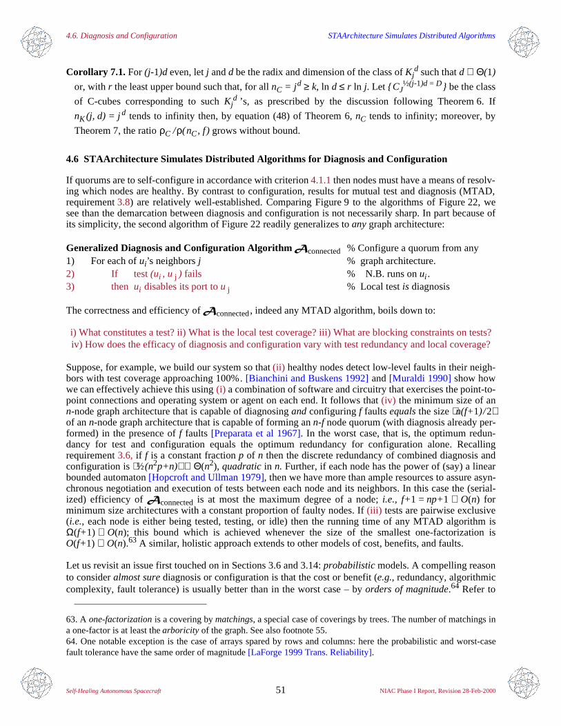
4.6. Diagnosis and Configuration STAArchitecture Simulates Distributed Algorithms
Self-Healing Autonomous Spacecraft 51 NIAC Phase I Report, Revision 28-Feb-2000
Corollary 7.1. For (j-1)d even, let j and d be the radix and dimension of the class of Kjd such that d ∈ Θ(1)
or, with r the least upper bound such that, for all nC = j d ≥ k, ln d ≤ r ln j. Let CJ½(j-1)d = D be the class
of C-cubes corresponding to such Kjd ’s, as prescribed by the discussion following Theorem 6. If
nK (j, d) = j d tends to infinity then, by equation (48) of Theorem 6, nC tends to infinity; moreover, by
Theorem 7, the ratio ρC /ρ(nC, f) grows without bound.
4.6 STAArchitecture Simulates Distributed Algorithms for Diagnosis and Configuration
If quorums are to self-configure in accordance with criterion 4.1.1 then nodes must have a means of resolv-ing which nodes are healthy. By contrast to configuration, results for mutual test and diagnosis (MTAD,requirement3.8) are relatively well-established. Comparing Figure 9 to the algorithms of Figure 22, wesee than the demarcation between diagnosis and configuration is not necessarily sharp. In part because ofits simplicity, the second algorithm of Figure 22 readily generalizes to any graph architecture:
Generalized Diagnosis and Configuration Algorithm $connected % Configure a quorum from any1) For each of ui’s neighbors j % graph architecture. 2) If test (ui , u j ) fails % N.B. runs on ui .3) then ui disables its port to u j % Local test is diagnosis
The correctness and efficiency of $connected, indeed any MTAD algorithm, boils down to:
i) What constitutes a test? ii) What is the local test coverage? iii) What are blocking constraints on tests?iv) How does the efficacy of diagnosis and configuration vary with test redundancy and local coverage?
Suppose, for example, we build our system so that (ii) healthy nodes detect low-level faults in their neigh-bors with test coverage approaching 100%. [Bianchini and Buskens 1992] and [Muraldi 1990] show howwe can effectively achieve this using (i) a combination of software and circuitry that exercises the point-to-point connections and operating system or agent on each end. It follows that (iv) the minimum size of ann-node graph architecture that is capable of diagnosing and configuring f faults equals the size n(f+1)/2of an n-node graph architecture that is capable of forming an n-f node quorum (with diagnosis already per-formed) in the presence of f faults [Preparata et al 1967]. In the worst case, that is, the optimum redun-dancy for test and configuration equals the optimum redundancy for configuration alone. Recallingrequirement 3.6, if f is a constant fraction p of n then the discrete redundancy of combined diagnosis andconfiguration is ½(n2p+n) ∈ Θ(n2), quadratic in n. Further, if each node has the power of (say) a linearbounded automaton [Hopcroft and Ullman 1979], then we have more than ample resources to assure asyn-chronous negotiation and execution of tests between each node and its neighbors. In this case the (serial-ized) efficiency of $connected is at most the maximum degree of a node; i.e., f+1 = np+1 ∈ O(n) forminimum size architectures with a constant proportion of faulty nodes. If (iii) tests are pairwise exclusive(i.e., each node is either being tested, testing, or idle) then the running time of any MTAD algorithm isΩ(f+1) ∈ O(n); this bound which is achieved whenever the size of the smallest one-factorization isO(f+1) ∈ O(n).63 A similar, holistic approach extends to other models of cost, benefits, and faults.
Let us revisit an issue first touched on in Sections 3.6 and 3.14: probabilistic models. A compelling reasonto consider almost sure diagnosis or configuration is that the cost or benefit (e.g., redundancy, algorithmiccomplexity, fault tolerance) is usually better than in the worst case – by orders of magnitude.64 Refer to
63. A one-factorization is a covering by matchings, a special case of coverings by trees. The number of matchings ina one-factor is at least the arboricity of the graph. See also footnote 55.64. One notable exception is the case of arrays spared by rows and columns: here the probabilistic and worst-casefault tolerance have the same order of magnitude [LaForge 1999 Trans. Reliability].
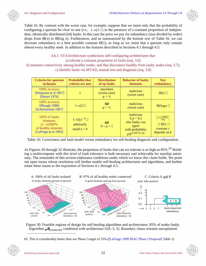
4.6. Diagnosis and Configuration STAArchitecture Delivers on Requirements 3.6 Through 3.8
Self-Healing Autonomous Spacecraft 52 NIAC Phase I Report, Revision 28-Feb-2000
Table 16. By contrast with the worst case, for example, suppose that we insist only that the probability ofconfiguring a quorum be close to one (i.e., ) in the presence of a constant proportion of indepen-dent, identically distributed (iid) faults. In this case the price we pay for redundancy (size divided by order)drops from Θ(n) to Θ(log n). Furthermore, and as summarized by the bottom row of Table 16, we candecrease redundancy to a best possible constant Θ(1), as long as we insist that a quorum only containalmost every healthy node. In addition to the features described in Sections 4.1 through 4.5:
4.6.1 STAArchitecture synthesizes self-configuring architectures thata) tolerate a constant proportion of faults (req. 3.6)
b) maintain connectivity among healthy nodes, and that disconnect healthy from faulty nodes (req. 3.7);c) identify faults via MTAD, mutual test and diagnosis (req. 3.8)
As Figures 30 through 32 illustrate, the proportion of faults that can we tolerate is as high as 85%.65 Build-ing a multicomputer with this level of fault tolerance is both necessary and achievable for starship auton-omy. The remainder of this section elaborates conditions under which we know this claim holds. We pointout open issues whose resolution will further enable self-healing architectures and algorithms, and furtherrelate these issues to the exposition of Sections 4.1 through 4.5.
Criteria for quorum inclusion
Probability that criteria are met
Distributionof np faults
Behavior of faulty elements
Testredundancy
100% accuracy [Preparata et al 1967]
[Hayes 1976]1
anywhere(worst case)
p < ½
malicious(worst case)
100% accuracy[Blough 1988]
[Scheinerman 1987]
iidp < ½
malicious(worst case)
100% of faultyelements;
(1 - ε)⋅100%of healthy elements[LaForge et al 1993]
arbitrarily
small ε > 0
iid0 < p < 1
maliciousif p < 0.5
else faulty can agree
with probabilityp⋅e-0.847/(1-p)
constant c
depends on ε
Table 16: Correctness and fault model versus redundancy for self-healing diagnosis and configuration.
65. This is considerably better than our Phase I target of 33% ([LaForge 1999 NIAC Phase I Proposal] Table 1)
Figure 30: Feasible regions of design for self-healing algorithms and architectures. 85% of nodes faulty.Algorithm $connected combined with architecture G(h; 5, 5). Boundary chaos remains unexplained.
1 o– 1( )
Θ n( )
1 o– 1( ) Θ nlog( )
1 O– n 1–( )c 3.4044+
pln–-------------------------
Θ∈ 1( )
A. 100% of all faults isolated B. 97% of all healthy nodes connected C. Criteria A and B% good elements missing from quorum
interconnectionredundancy / 4h
prob. falsepositive
020
4060
80
100
135791113151719210.00.1
0.20.3
% faulty elements present in quorum
interconnectionredundancy / 4h
prob. falsepositive
020
4060
80
100
135791113151719
210.0
0.10.2
0.3
0.2
0.1
0.0
interconnectionredundancy
3 5 71
prob. false positive
A ∩ B
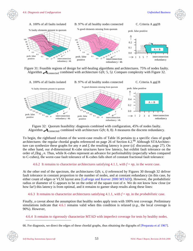
4.6. Diagnosis and Configuration Unfinished Business
Self-Healing Autonomous Spacecraft 53 NIAC Phase I Report, Revision 28-Feb-2000
To begin, the righthand column of the worst-case results of Table 16 pertains to a specific class of grapharchitectures: the regular chordal graphs referenced on page 26 of Section 4.2.66 Although STAArchitec-ture can synthesize these graphs for any n and f, the resulting latency is poor (cf. discussion, page 27). Onthe other hand, our d-dimensional K-cube structures have low latency, but exhibit fault tolerance on theorder of j⋅log j n. Thus, while K-cubes represent an advance for performability (especially when comparedto C-cubes), the worst-case fault tolerance of K-cubes falls short of constant fractional fault tolerance:
4.6.2 It remains to characterize architectures satisfying 4.1.1, with f = np, in the worst case.
At the other end of the spectrum, the architectures G(h; s, t) referenced by Figures 30 through 32 deliverfault tolerance in constant proportion to the number of nodes, and at constant redundancy (in this case, byeither count of edges or VLSI layout area [LaForge and Korver 2000 MTAD]). However, the probabilisticradius or diameter of G appears to be on the order of the square root of n. We do not know how close (orhow far!) this latency is from optimal, and it remains to garner sharp results along these lines:
4.6.3 It remains to characterize architectures satisfying 4.1.1, with f = np, in the probabilistic case.
Finally, a caveat about the assumption that healthy nodes apply tests with 100% test coverage. Preliminarysimulations indicate that 4.6.1 remains valid when this condition is relaxed (e.g., the local coverage is90%). However,
4.6.4 It remains to rigorously characterize MTAD with imperfect coverage for tests by healthy nodes.
Figure 31: Feasible regions of design for self-healing algorithms and architectures. 75% of nodes faulty.Algorithm $connected combined with architecture G(h; 5, 5). Compare complexity with Figure 32.
Figure 32: Quorum feasibility: diagnosis combined with configuration, 45% of nodes faulty.Algorithm $connected combined with architecture G(h; 8, 8). h measures the discrete redundancy.
66. For diagnosis, we direct the edges of these chordal graphs, thus obtaining the digraphs of [Preparata et al 1967].
A. 100% of all faults isolated B. 97% of all healthy nodes connected C. Criteria A and B
% good elements missing from quorum
interconnectionredundancy / 4h
prob. falsepositive
020
4060
80
100
135
79
1113
15170.0
0.10.2
0.3
interconnectionredundancy / 4h
% faulty elements present in quorum
prob. falsepositive
020
4060
80
100
13
57
911
1315
170.00.1
0.20.3
0.2
0.1A ∩ B
0.0
interconnectionredundancy
3 5 71
prob. false positive
interconnectionredundancy / 4h
% faulty elements present in quorum
prob. falsepositive 40.0
010
12
30.1
0.20.3
0.40.5
3040
5060
20
% good elements missing from quorum
interconnectionredundancy / 4h
prob. falsepositive
010
2030
4050
60
1
2
3
40.00.1
0.20.3
0.40.5
interconnectionredundancy
0.4
0.2
prob. false positive
0.0
A ∩ B
21 43
A. 100% of all faults isolated B. 97% of all healthy nodes connected C. Criteria A and B
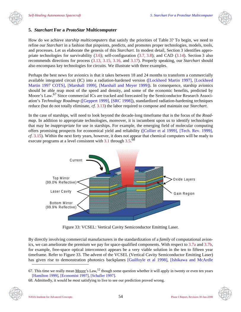
Self-Healing Autonomous Spacecraft 5. Starchart For a ProtoStar Multicomputer
NASA Institute for Advanced Concepts 54 Phase I Report, Revision 30-Jan-2000
5. Starchart For a ProtoStar Multicomputer
How do we achieve starship multicomputers that satisfy the priorities of Table 3? To begin, we need torefine our Starchart in a fashion that pinpoints, predicts, and promotes proper technologies, models, tools,and processes. Let us elaborate the genesis of this Starchart. In modest detail, Section 3 identifies appro-priate technologies for survivability (3.6); self-configuration (3.7, 3.8); and CAD (3.14). Section 3 alsorecommends directions for process (3.13, 3.15, 3.16, and 3.17). Properly speaking, our Starchart shouldalso encompass key technologies for circuits. We illustrate with three examples.
Perhaps the best news for avionics is that it takes between 18 and 24 months to transform a commerciallyavailable integrated circuit (IC) into a radiation-hardened version ([Lockheed Martin 1997], [LockheedMartin 1997 COTS], [Marshall 1999], [Marshall and Meyer 1999]). In consequence, starship avionicsshould be able reap most of the speed and density, and some of the economic benefits, predicted byMoore’s Law.67 Since commercial ICs are tracked and forecasted by the Semiconductor Research Associ-ation’s Technology Roadmap ([Geppert 1999], [SRC 1998]), standardized radiation-hardening techniquesreduce (but do not totally eliminate, cf. 3.13) the labor required to compose and maintain our Starchart.
In the case of starships, will need to look beyond the decade-long timeframe that is the focus of the Road-map. In addition to appropriate technologies, moreover, it is incumbent upon us to identify technologiesthat may be inappropriate for use in starships. For example, the emerging field of molecular computingoffers promising prospects for economical yield and reliability ([Collier et al 1999], [Tech. Rev. 1999],cf. 3.15). Within the next forty years, however, it does not appear that chemical computers will be ready toexecute programs at a level consistent with 3.1 through3.5.68
By directly involving commercial manufacturers in the standardization of a family of computational avion-ics, we can ameliorate the premium we pay for space-qualified components. With respect to 3.7a and 3.7b,for example, free-space optical interconnect appears be a very viable solution in the ten to fifteen yeartimeframe. Refer to Figure 33. The advent of the VCSEL (Vertical Cavity Semiconductor Emitting Laser)has given rise to demonstration photonics backplanes [Guilfoyle et al 1998], [Ishikawa and McArdle
67. This time we really mean Moore’s Law,12 though some question whether it will apply in twenty or even ten years[Hamilton 1999], [Economist 1997], [Schaller 1997].
Figure 33: VCSEL: Vertical Cavity Semiconductor Emitting Laser.
68. Admittedly, it would be most satisfying to live to see our prediction proved wrong.
C urren t
Top M irro r(99 .0% R e flec tive )
Laser C av ity
B o ttom M irro r(99 .9% R e flec tive )
O xide Layers
G a in R eg ion
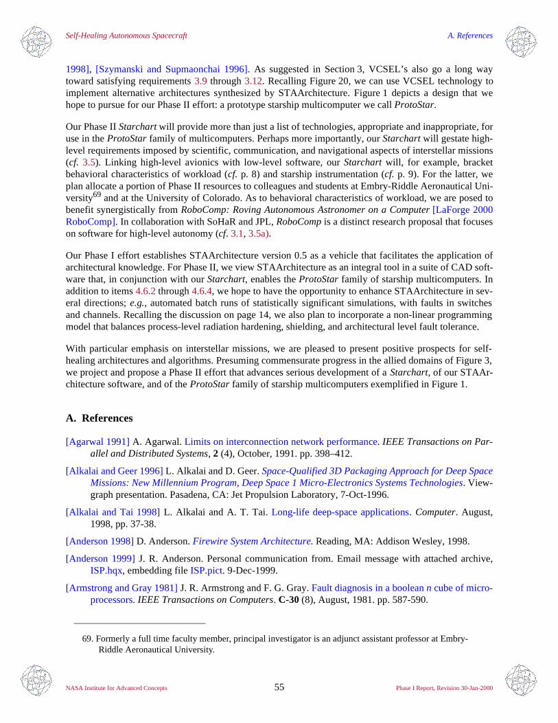
Self-Healing Autonomous Spacecraft A. References
NASA Institute for Advanced Concepts 55 Phase I Report, Revision 30-Jan-2000
1998], [Szymanski and Supmaonchai 1996]. As suggested in Section 3, VCSEL’s also go a long waytoward satisfying requirements 3.9 through 3.12. Recalling Figure 20, we can use VCSEL technology toimplement alternative architectures synthesized by STAArchitecture. Figure 1 depicts a design that wehope to pursue for our Phase II effort: a prototype starship multicomputer we call ProtoStar.
Our Phase II Starchart will provide more than just a list of technologies, appropriate and inappropriate, foruse in the ProtoStar family of multicomputers. Perhaps more importantly, our Starchart will gestate high-level requirements imposed by scientific, communication, and navigational aspects of interstellar missions(cf. 3.5). Linking high-level avionics with low-level software, our Starchart will, for example, bracketbehavioral characteristics of workload (cf. p. 8) and starship instrumentation (cf. p. 9). For the latter, weplan allocate a portion of Phase II resources to colleagues and students at Embry-Riddle Aeronautical Uni-versity69 and at the University of Colorado. As to behavioral characteristics of workload, we are posed tobenefit synergistically from RoboComp: Roving Autonomous Astronomer on a Computer [LaForge 2000RoboComp]. In collaboration with SoHaR and JPL, RoboComp is a distinct research proposal that focuseson software for high-level autonomy (cf. 3.1, 3.5a).
Our Phase I effort establishes STAArchitecture version 0.5 as a vehicle that facilitates the application ofarchitectural knowledge. For Phase II, we view STAArchitecture as an integral tool in a suite of CAD soft-ware that, in conjunction with our Starchart, enables the ProtoStar family of starship multicomputers. Inaddition to items 4.6.2 through 4.6.4, we hope to have the opportunity to enhance STAArchitecture in sev-eral directions; e.g., automated batch runs of statistically significant simulations, with faults in switchesand channels. Recalling the discussion on page 14, we also plan to incorporate a non-linear programmingmodel that balances process-level radiation hardening, shielding, and architectural level fault tolerance.
With particular emphasis on interstellar missions, we are pleased to present positive prospects for self-healing architectures and algorithms. Presuming commensurate progress in the allied domains of Figure 3,we project and propose a Phase II effort that advances serious development of a Starchart, of our STAAr-chitecture software, and of the ProtoStar family of starship multicomputers exemplified in Figure 1.
A. References
[Agarwal 1991] A. Agarwal. Limits on interconnection network performance. IEEE Transactions on Par-allel and Distributed Systems, 2 (4), October, 1991. pp. 398–412.
[Alkalai and Geer 1996] L. Alkalai and D. Geer. Space-Qualified 3D Packaging Approach for Deep SpaceMissions: New Millennium Program, Deep Space 1 Micro-Electronics Systems Technologies. View-graph presentation. Pasadena, CA: Jet Propulsion Laboratory, 7-Oct-1996.
[Alkalai and Tai 1998] L. Alkalai and A. T. Tai. Long-life deep-space applications. Computer. August,1998, pp. 37-38.
[Anderson 1998] D. Anderson. Firewire System Architecture. Reading, MA: Addison Wesley, 1998.
[Anderson 1999] J. R. Anderson. Personal communication from. Email message with attached archive,ISP.hqx, embedding file ISP.pict. 9-Dec-1999.
[Armstrong and Gray 1981] J. R. Armstrong and F. G. Gray. Fault diagnosis in a boolean n cube of micro-processors. IEEE Transactions on Computers. C-30 (8), August, 1981. pp. 587-590.
69. Formerly a full time faculty member, principal investigator is an adjunct assistant professor at Embry-Riddle Aeronautical University.
Self-Healing Autonomous Spacecraft A. References
NASA Institute for Advanced Concepts 56 Phase I Report, Revision 30-Jan-2000
[Artin 1975] M. Artin. Linear Algebra and Group Theory. Massachusetts Institute of Technology: notesfor course 18.701, 1975.
[Aviation Week 1997] Ariane 5 report details software design errors. Aviation Week and Space Technol-ogy. 9-Sep-1997. pp. 79-81.
[Avizienis 1967] A. Avizienis. Design of fault-tolerant computers. 1967 Fall Joint Computer Conference,AFIPS Conference Proceedings, 31. Washington, D.C.: Thompson-Brooks, 1967. pp. 733-743.
[Avizienis 1997] A. Avizienis. Toward systematic design of fault-tolerant systems. Computer. April, 1997.pp. 51-58.
[Avizienis 1999] A. Avizienis. The hundred year spacecraft. Proceedings, First NASA/DOD Workshop onEvolvable Hardware. Pasadena, CA: Jet Propulsion Laboratory, 19, 20, 21-July-1999. pp. 233-239.
[Banerjee et al 1986] P. Banerjee, S-Y Kuo, and W. K. Fuchs. Reconfigurable cube-connected cyclesarchitectures. Proceedings, 16th International Symposium on Fault Tolerant Computing. July, 1986,pp. 286-291.
[Barry 1998] R. C. Barry. X2000 Fault Protection Approach, Plan. Viewgraph presentation. Pasadena,CA: Jet Propulsion Laboratory, 26-Feb-1998.
[Bendetto 1998] J. M. Bendetto. Economy-class ion-defying ICs in orbit. IEEE Spectrum. March, 1998.pp. 36-41.
[Bernard 1999] D. E. Bernard. RAX Update and Schedule. Email message. 24-May-1999.
[Bianchini and Buskens 1992] R. P. Bianchini, Jr. and R. W. Buskens. Implementation of on-line distrib-uted systems-level diagnosis theory. IEEE Transactions on Computers, 41 (5), May, 1992.
[Biggs 1993] N. Biggs. Algebraic Graph Theory. New York: Cambridge University Press, 1993. 2nd ed.
[Blough 1988] D. M. Blough. Fault Detection and Diagnosis in Multiprocessor Systems. Ph.D. disserta-tion. Baltimore: Johns Hopkins University, 1988.
[Bollabás, 1978] B. Bollabás. Extremal Graph Theory. London: Academic Press, 1978.
[Braham 1999] R. Braham. Space: the wheel turns. In Technology 1999 analysis and forecast: aerospaceand military, IEEE Spectrum. January, 1999. pp. 73-78.
[Bryant et al 1989] W. H. Bryant, R. K. Iyer, J. B. Dugan, W. L. Heimerdinger, J. Lala, J. Peterson, B.Randell. Computer-aided design of dependable mission critical systems. Report of a panel discus-sion, in Digest of Papers: 19th Symposium on Fault-Tolerant Computing Systems. Los Alamitos,CA: IEEE Computer Society Press, 1989. pp. 416-420.
[Broad 1999] W. J. Broad. Experts warn of Mars on the cheap. New York Times. 8-Dec-1999. p. A15.
[Butler et al 1999] R. P. Butler, G. W. Marcy, D. A. Fischer, T. W. Brown, A. R. Contos, S. G. Korzennik,P. Nisenson, and R. W. Noyes. Evidence for multiple companions to Upsilon Andromedae. Astro-physical Journal. Submitted, 1999. Online at http://cfa-www.harvard.edu/afoe/ and athttp://www.physics.sfsu.edu/~garcy/planetsearch/upsand/upsand.html.
[Carson 1996] J. Carson. The emergence of stacked 3D silicon and its impact on microelectronics systemintegration. Proceedings, IEEE International Conference on Innovative Systems in Silicon.S. Tewksbury and G. Chapman, eds. IEEE Press, 1996. pp. 1-8.
[Cash 1999] W. Cash, personal communication with. NASA Institute for Advanced Concepts FellowsMeeting. 9-Nov-1999.
[Cash 1999 X-File] W. Cash. X-Ray Interferometry: The Future of X-Ray Astronomy. Viewgraph presenta-
Self-Healing Autonomous Spacecraft A. References
NASA Institute for Advanced Concepts 57 Phase I Report, Revision 30-Jan-2000
tion. Atlanta: NASA Institute for Advanced Concepts Fellows Meeting, 8, 9-Nov-1999. Online athttp://peaches.niac.usra.edu/library/nov99_mtng/cash_nov99.pdf.
[Cassanova 1999] R. Cassanova. Opening Remarks. Viewgraph presentation. Atlanta: NASA Institute forAdvanced Concepts Fellows Meeting, 8, 9-Nov-1999. Online athttp://peaches.niac.usra.edu/library/nov99_mtng/cassanova_nov99.pdf.
[Chartrand and Lesniak 1986] G. Chartrand and L. Lesniak. Graphs and Digraphs. Belmont, CA: Wad-sworth, Inc, 1986. 2nd ed.
[Chau 1998] S. Chau. X2000 Core Avionics Peer Review: Characteristics of a Reliable Bus. Viewgraphpresentation. Pasadena, CA: Jet Propulsion Laboratory, 17-Apr-1998. Online at http://knowl-edge.jpl.nasa.gov/adssdlib/.
[Chau 1998 PDR] S. Chau. Backup: Upstream Connection Failure. Viewgraph presentation, X2000 Pre-liminary Design Review. Pasadena, CA: Jet Propulsion Laboratory, 18, 19, 20-Aug-1998.
[Chau 1999] S. Chau. Personal communication. 10-Dec-1999.
[Chau and Holmberg 1998] S. Chau and E. Holmberg. X2000 Core Avionics Peer Review: CDH SlicesDescription. Viewgraph presentation. Pasadena, CA: Jet Propulsion Laboratory, 17-Apr-1998.Online at http://knowledge.jpl.nasa.gov/adssdlib/.
[Chen and Upadhyaya 1993] Y-Y Chen and S. J. Upadhyaya. Reliability, reconfiguration, and spare allo-cated issues in binary tree architectures based on multiple-level redundancy. IEEE Transactions onComputers, 42 (6), June, 1993. pp. 713–723.
[Clark 1998] D. Clark. Defect-tolerant computer. Computer. August, 1998. p. 27.
[Cole 1999] J. Cole. Personal communication. Atlanta: NASA Institute for Advanced Concepts FellowsMeeting, 8-Nov-1999.
[Collier et al 1999] C. P. Collier, E. W. Wong, M. Belohradsky, F. M. Raymo, J. F. Stoddart, P. J. Kuekes,R. S. Williams, J. R. Heath. Electronically configurable molecular-based logic gates. Science, 285.16-Jul-1999. pp. 391–394.
[Comtet 1974] L. Comtet. Advanced Combinatorics. Dordrecht, Holland: R. Reidel Publishing, 1974. 2nded.
[Culbertson et al 1996] B. Culbertson, R. Amerson, R. Carter, P Kuekes, and G. Snider. The Teramac cus-tom computer: extending the limits with defect tolerance. Proceedings, 1996 IEEE InternationalSymposium on Defect and Fault Tolerance in VLSI Systems.
[Culbertson et al 1997] B. Culbertson, R. Amerson, R. Carter, P Kuekes, and G. Snider. Defect toleranceon the Teramac custom computer. Proceedings, 1997 IEEE Symposium on FPGA’s for CustomComputing Machines. pp. 116-123.
[Das et al 1993] A. Das, K. Thulasiraman, V. K. Agarwal, K. B. Lakshmanan. Multiprocessor fault diagno-sis under local constraints. IEEE Transactions on Computers, 42 (8), August 1993. pp. 984-988.
[Dornheim 1998] M. A. Dornheim. Deep Space 1 launch slips three months. Aviation Week and SpaceTechnology. 27-Apr-1998. p. 39.
[Dumullin 1999] J. Dumullin. Apollo 17 (33). Kennedy Space Center Historical Archives. 23-Jun-1999.Online at http://www.ksc.nasa.gov/history/apollo/apollo-17/apollo-17.html.
[Dutt and Hayes 1990] S. Dutt and J. P. Hayes. On designing and reconfiguring k-fault-tolerant tree archi-tectures. IEEE Transactions on Computers, 39 (4), April, 1990. pp. 490–503.
Self-Healing Autonomous Spacecraft A. References
NASA Institute for Advanced Concepts 58 Phase I Report, Revision 30-Jan-2000
[Dvorak 1998] D. L. Dvorak. Revisions for MDS prototype. Pasadena, CA: Jet Propulsion Laboratoryinternal document, 7-Jul-1998.
[Dvorak 1999] D. L. Dvorak, personal communication with. 30-Nov-1999.
[Dvorak and Doyle 1998] D. L. Dvorak and R. J. Doyle. Robo-Scientist. Pasadena, CA: Memorandum toJet Propulsion Laboratory Chief Scientist Moustafa Chahine, 11-Jun-1998.
[Economist 1997] Not Moore's Law. The Economist. 12-Jul-1997. p. 72.
[Eldred 1997] D. B. Eldred. DS1 Flight Software Integration: Causes for Schedule Slip. Viewgraph pre-sentation, Pasadena, CA: Jet Propulsion Laboratory, 26-Feb-1997, revised 9-Aug-1997.
[Elfun 1977] Schenectady Elfun Society. The General Electric Story, A Photo History, Volume 2: TheSteinmetz Era, 1892–1923. Schenectady, NY: Elfun Hall of History Publications, 1977.
[Feather 1999] M. Feather. Personal communication from. Email message. 14-Feb-1999.
[Foust 1999] J. Foust. E.T. – don't call home: a spacecraft thinks for itself. Technology Review.September / October, 1999. p 36.
[Gavit 1999] S. A. Gavit. Interstellar Probe. Viewgraph presentation8_991ISPSummary_PublicPackage.ppt, Pasadena, CA: Jet Propulsion Laboratory, 26-Aug-1999.
[Geppert 1998] L. Geppert. The age of copper. In Technology 1998 analysis and forecast: solid state, IEEESpectrum. January, 1998. pp. 23-28.
[Geppert 1999] L. Geppert. The 100-million transistor IC. IEEE Spectrum. July, 1999, pp. 23-24.
[Glass 1997] R. Glass. Telling good numbers from bad ones. IEEE Software. July/Aug-1997. pp. 15-19.
[Gluck 1999] P. R. Glück. Remote Agent Operational (2 Day Test). Email message. 17-May-1999.
[Goldin et al 1998] D. S. Goldin, S. L. Venneri, and A. K. Voor. Beyond incremental change. Computer.October, 1998. pp. 31-40.
[Goldsmith 1999] D. Goldsmith. Voyage to the Milky Way: The Future of Space Exploration. New York:TV Books, 1999.
[Guiar 1998] C. N. Guiar. X2000 High Level Driving Technical Requirements/Constraints. Viewgraphpresentation, Core Avionics Peer Review. Pasadena, CA: Jet Propulsion Laboratory, 11-Jun-1998.
[Guilfoyle et al 1998] P. S. Guilfoyle, J. M. Hessenbruch, and R. V. Stone. Free-space interconnects forhigh-performance optoelectric switching. Computer. February, 1998. pp. 69-75.
[Halvorson 1999] T. Halvorson. Faulty wire harness brought down Titan 4a rocket. Florida Today, SpaceOnline: http://www.flatoday.com/space/explore/stories/1999/011699f.htm. 16-Jan-1999.
[Haverkort and Niemegeers 1996] B. R. Haverkort and I. G. Niemegeers. Performability modelling toolsand techniques. Performance Evaluation, 25. 1996. pp. 17-40.
[Hecht and Fiorentino 1988] M. Hecht and E. Fiorentino. Causes and effects of spacecraft failures. Qualityand Reliability Engineering International, 4 (11), August, 1988. pp. 12-19.
[Hamilton 1999] S. Hamilton. Taking Moore’s Law into the next century. Computer. January, 1999.pp. 43-48.
[Harris] Harris Semiconductor Quality and Reliability Manual. Intersil Corporation (formerly HarrisSemiconductor) reliability white paper. Online at http://rel.semi.harris.com/docs/rel/.
[Hayes 1976] J. P. Hayes. A graph model for fault tolerant computing systems. IEEE Transactions on
Self-Healing Autonomous Spacecraft A. References
NASA Institute for Advanced Concepts 59 Phase I Report, Revision 30-Jan-2000
Computers, C-25 (9), September, 1976. pp. 875-884.
[Hopcroft and Ullman 1979] J. E. Hopcroft and J. D. Ullman. Introduction to Automata Theory, Lan-guages, and Computation. Reading, MA: Addison-Wesley, 1979.
[Hotz 1999 Nov] R. L. Hotz. String of missteps doomed orbiter; JPL found at fault. Los Angeles Times.11-Nov-1999. p. A1.
[Hotz 1999 Dec] R. L. Hotz. Are failed Mars probes price of cost-cutting? Los Angeles Times online,http://www.latimes.com/news/science/science/19991226/t000117877.html. 26-Dec-1999.
[Hunter 1997] D. J. Hunter. X2000 Design, Implementation, and Cost Review: First Delivery Project:Electronic Packaging. Viewgraph presentation. Pasadena, CA: Jet Propulsion Laboratory,11-through 13-Mar-1997. Online at http://knowledge.jpl.nasa.gov/adssdlib/.
[Hunter 1998] D. J. Hunter. X2000 Peer Review: Horizontal Mounted Cube (HMC) and Integrated Avion-ics System (IAS), Electronic Packaging Architecture. Viewgraph presentation. Pasadena, CA: JetPropulsion Laboratory, 16-Jul-1998.
[Irwin and Narayanan 1999] M. J. Irwin and V. Narayanan. A transition sensitive, architectural levelpower analysis approach. IEEE Computer Society Technical Committee on VLSI, Technical Bulletin.Summer 1999. pp. 6-11.
[Ishikawa and McArdle 1998] M. Ishikawa and N. McArdle. Optically interconnected parallel computingsystems. Computer. February, 1998. pp. 61-68.
[Jezequel and Meyer 1997] J.-M. Jezequel and B. Meyer. Design by contract: the lessons of Ariane. Com-puter. January, 1997. pp. 129-130.
[JPL 1994 Pathfinder Software] Mars Pathfinder AIM Flight Software. Pasadena, CA: Jet Propulsion Lab-oratory internal design document, 28-Nov-1994.
[JPL DS1 Press Release] Computer Program Assumes Spacecraft Command. Pasadena, CA: Jet Propul-sion Laboratory, Media Relations Office press release. 17-May-1999.
[JPL 1999 Voyager] Voyager Home Page. Pasadena, CA: Jet Propulsion Laboratory documentation,online at http://vraptor.jpl.nasa.gov/voyager/vimdesc.html. August, 1999.
[Kammash 1999] T. Kammash. Anti-proton Driven Magnetically Insulated Inertial Fusion PropulsionSystem. Viewgraph presentation. Atlanta: NASA Institute for Advanced Concepts Fellows Meeting,8, 9-Nov-1999. Online at http://peaches.niac.usra.edu/library/nov99_mtng/kammash_nov99.pdf.
[Kaufmann and Freedman 1999] W. J. Kaufmann III and R. A. Freedman. Universe. New York: W. H.Freeman and Company, 1999. Fifth edition.
[Knowledge Adventure 1999] Knowledge Adventure. Connect the dots. Online at http://www.kid-space.com/kids/connect_dots.
[Koshgoftaar et al 1998] T. M. Koshgoftaar, E. B. Allen, R. Halstead, G. P. Trio, R. M. Flass. Using pro-cess history to predict software quality. Computer. April, 1998. pp. 66-72.
[Kwan and Toida 1981] C.-L. Kwan and S. Toida. Optimal fault-tolerant realizations of some classes ofhierarchical tree systems. 11th Annual Symposium on Fault-Tolerant Computing. 24-26 June, 1981.New York: IEEE Press. pp. 176-178.
[LaForge 1994] L. E. LaForge. What designers of wafer scale systems should know about local sparing.Proceedings, Sixth Annual IEEE International Conference on Wafer Scale Integration. Piscataway,N.J.: IEEE Press, 1994. pp 106-131.
Self-Healing Autonomous Spacecraft A. References
NASA Institute for Advanced Concepts 60 Phase I Report, Revision 30-Jan-2000
[LaForge 1997 CVS] L. E. LaForge. Deep Space 1: flight software CVS logging and tagging.Pasadena, CA: Jet Propulsion Laboratory internal specification, 26-Sep-1997.
[LaForge 1997 DS1] L. E. LaForge. Tracking and Analysis of Soft Failures and Faults for Deep Space 1.Viewgraph presentation. Pasadena, CA: Jet Propulsion Laboratory, 26-Sep-1997.
[LaForge 1999 NIAC Phase I Proposal] L. E. LaForge. Architectures and Algorithms for Self-HealingAutonomous Spacecraft. NASA Institute for Advanced Concepts Phase I Proposal. 31-Jan-1999.
[LaForge 1999 JPL D-16485] L. E. LaForge. Fault tolerant physical interconnection of X2000 computa-tional avionics. Pasadena, CA: Jet Propulsion Laboratory, document number JPL D-16485.28-Aug-1998, revised 18-Oct-1999. Online at http://knowledge.jpl.nasa.gov/adssdlib/ and athttp://www.ec.erau.edu/cce/centers/faculty/laforgel/Current-and-Recent-Research/NASA-ASEE/.
[LaForge 1999 Trans. Computers] L. E. LaForge. Configuration of locally spared arrays in the presence ofmultiple fault types. IEEE Transactions on Computers, 48 (4). April, 1999. pp. 398-416.
[LaForge 1999 Trans. Reliability] L. E. LaForge. What designers of microelectronic systems should knowabout arrays spared by rows and columns. IEEE Transactions on Reliability. Submitted November,1999.
[LaForge 2000 RoboComp] L. E. LaForge. RoboComp: Roving Autonomous Astronomer on a Computer.Notice of intent to propose. Advanced Cross-Enterprise Technology Development for NASA Mis-sions. NRA 99-OSS-05, Topic A.5, Thinking Space Systems. 5-Jan-2000.
[LaForge 2000 Starship Avionics] L. E. LaForge. Self-healing avionics for starships. 2000 IEEE Aero-space Conference. 18-Mar-2000.
[LaForge and Korver 2000 Graph Fault Tolerance] L. E. LaForge and K. F. Korver. Graph-theoretic faulttolerance for spacecraft bus avionics. 2000 IEEE Aerospace Conference. 18-Mar-2000
[LaForge and Korver 2000 MTAD] L. E. LaForge and K. F. Korver. Mutual test and diagnosis: architec-tures and algorithms for spacecraft avionics. 2000 IEEE Aerospace Conference. 18-Mar-2000.
[LaForge et al 1993] L. E. LaForge, K. Huang, and V. K. Agarwal. Almost sure diagnosis of almost everygood element. IEEE Transactions on Computers, 43 (3). March, 1994. pp. 295-305.
[LaForge et al 1999] L. E. LaForge, C. Cassell, M. Hecht, K. F. Korver, D. D. Carlson. Avionics and Soft-ware for a Starship to Alpha Centauri. Viewgraph presentation Avionics-and-Software-for-a-Mis-sion-to-Alpha-Centauri.ppt. Pasadena, CA: Jet Propulsion Laboratory, 25-Aug-1999.
[Lalli 1998] V. R. Lalli. Space-system reliability: a historical perspective. IEEE Transactions on Reliabil-ity, 47 (3). September, 1998. pp. 355-360.
[LaPointe 1999] M. R. LaPointe. Primary Propulsion for Piloted Deep Space Exploration. Viewgraph pre-sentation. Atlanta: NASA Institute for Advanced Concepts Fellows Meeting, 8, 9-Nov-1999. Onlineat http://peaches.niac.usra.edu/library/nov99_mtng/lapointe_nov99.pdf.
[Larson and Wertz 1995] W. J. Larson and J. R. Wertz. Space Mission Analysis and Design. Boston: Klu-wer Academic Publishers, 1995.
[Leighton and Leiserson 1985] T. Leighton and C. E. Leiserson. Wafer-scale integration of systolic arrays.IEEE Transactions on Computers, 34 (5). May, 1985. pp. 448-461.
[Lee and Cong 1997] T-C Lee and J. Cong. The new line in IC design. IEEE Spectrum. March, 1997. pp.52-58.
[Lewis and Postol 1997] G. N. Lewis and T. A. Postol. Future challenges to ballistic missile defense. IEEESpectrum. September, 1997. pp. 60-68.
Self-Healing Autonomous Spacecraft A. References
NASA Institute for Advanced Concepts 61 Phase I Report, Revision 30-Jan-2000
[Lockheed Martin 1997] The RAD6000 Flight Computer. Technical product description. Lockheed MartinCorporation. 29-Aug-1997.
[Lockheed Martin 1997 COTS] Radiation Hardened COST-based 32-bit Microprocessor. Technical prod-uct description. Lockheed Martin Corporation. 1997.
[Lockheed Martin 1999] Rad-Lite Product Discussion. Viewgraph presentation B5346.ppt. LockheedMartin Corporation. January, 1999.
[Lowry 1998] M. R. Lowry. Component-based reconfigurable systems. Computer. April, 1998. pp. 44-45.
[Marcopulos 1998] T. Marcopulos. Faster, better, cheaper space exploration. IEEE Spectrum. August,1998. pp. 68-74.
[Marcus 1998] S. J. Marcus. Grand illusion: the risks of Cassini. IEEE Spectrum. March, 1998. pp. 58-65.
[Marshall 1999] J. Marshall. Personal communication. 8-Oct-1999.
[Marshall and Meyer 1999] J. Marshall and D. Meyer. Personal communication. 12-Dec-1999.
[McDermid and Talbert 1998] J. McDermid and N. Talbert. The cost of COTS. Computer. June, 1998.pp. 46-52.
[McNutt et al 1997] R. L. McNutt, Jr, R. E. Gold, E. C. Roelof, L. J. Zanetti, E. L. Reynolds,R. W. Farquhar, D. A. Gurnett, and W. S. Kurth. A SOLE/AD ASTRA: from the sun to the stars.Journal of the British Interplanetary Society, 50. 1997. pp. 463-474.
[McNutt 1999] R. L. McNutt, Jr. A Realistic Interstellar Explorer. NASA Institute for Advanced ConceptsPhase I final report, May, 1999. Online at www.niac.usra.edu/studies/9801/9801Final/McNuttFi-nal.pdf.
[Meyer 1999] B. Meyer. Every little bit counts: toward more reliable software. Computer. November,1999. pp. 131-133.
[Milky Way 1999] Voyage to the Milky Way. Video documentary, Thomas Lucas Productions, 1999.
[Millis 1997] M. G. Millis. The challenge to create the space drive. Journal of Propulsion and Power.13 (5), September / October, 1997. pp. 577 - 682. Online athttp://www.lerc.nasa.gov/www/bpp/TM-107289.htm.
[Moore and Shannon 1956] E. F. Moore and C. E. Shannon. Reliable circuits using less reliable relays,part I. Journal of the Franklin Institute, 262. September, 1956. pp. 191-208.
[Morrison and Schmidt 1999] D. Morrison and G. K. Schmidt, editors. Astrobiology Roadmap. NASAAmes Research Center document. 4-Jan-1999. Online at http://astrobiology.arc.nasa.gov/roadmap/.
[Muirhead 1996 Pathfinder Design] B. K. Muirhead. Mars Pathfinder flight system design and implemen-tation. Proceedings, 1996 IEEE Aerospace Conference, 4. Snowmass at Aspen: 1-8 Feb 1996.pp. 191-205.
[Muirhead 1996 Pathfinder Test] B. K. Muirhead. Mars Pathfinder flight system integration and test. Pro-ceedings, 1996 IEEE Aerospace Conference, 4. Snowmass at Aspen: 1-8 Feb 1996.
[Munson and Werries 1996] J. C. Munson and D. S. Werries. Measuring software evolution. Proceedings,1996 IEEE International Software Metrics Symposium. IEEE Computer Society Press. pp. 41-51.
[Muraldi 1990] F. Muraldi. A New Procedure for Weighted Random Built-in Self Test. Ph.D. dissertation,Montreal: Department of Electrical Engineering, McGill University, March, 1990.
[Murty and Vijayan 1964] U. S. R. Murty and K. Vijayan. On accessibility in graphs. Sakhya Ser. A, Vol
Self-Healing Autonomous Spacecraft A. References
NASA Institute for Advanced Concepts 62 Phase I Report, Revision 30-Jan-2000
26, 1964. pp. 299 - 302.
[Nabli and Sericola 1996] H. Nabli and B. Sericola. Performability analysis: a new algorithm. IEEE Trans-actions on Computers, 45 (4). April, 1996. pp. 491-494.
[NASA 1999] High integrity systems and algorithms. Topic 1.04, in SBIR: Small Business InnovationResearch, 1999 Program Solicitation. National Aeronautics and Space Administration. Openingdate: 24-Apr-1999.
[Neumann 1996] P. G. Neumann. Using formal methods to reduce risk. Communications of the ACM,39 (7). July, 1996. p. 114.
[NIAC 1999 Agenda] NASA Institute for Advanced Concepts. NIAC Fellows Meeting Agenda.8, 9-Nov-1999. Online at http://www.niac.usra.edu/library/nov99_mtng/nov99_agenda.pdf.
[NIAC 1999 Scope] NASA Institute for Advanced Concepts. Scope of NIAC Call for Proposals. Online athttp://peaches.niac.usra.edu/library/challenges/challenges-final.pdf.
[Nikora et al 1998] A. P. Nikora, N. F. Schneidewind, and J. C. Munson. IV&V issues in achieving highreliability and safety in critical control system software, final report. Pasadena, CA: Jet PropulsionLaboratory, document number D-15740, 19-Jan-1998.
[Nordley 1998] G. Nordley. Don’t rule out interstellar probes. SETI League Publications. 28-Feb-1998.Online at http://seti1.setileague.org/articles/probes.htm.
[Norvig 1999] P. Norvig. Personal communication. 2-Aug-1999.
[Oberg 1998] J. Oberg. Shuttle-Mir’s lessons for the International Space Station. IEEE Spectrum. June,1998. pp. 28-37.
[Ore 1962] O. Ore. Theory of Graphs. Providence: American Mathematical Society Publications, 1962.
[Pedder 1993] D. J. Pedder. Interconnection technologies for multichip assemblies (ITMA) – a UK infor-mation technology engineering directorate hybrid wafer scale project. Proceedings, Fifth Annual IEEEInternational Conference on Wafer Scale Integration. Piscataway, N.J.: IEEE Press, 1993. pp. 95-106.
[Pickering 1999] K. A. Pickering. A Christopher Columbus Timeline. 12-Oct-1999. Online atwww1.minn.net/~keithp/cctl.htm.
[Preparata et al 1967] F. Preparata, G. Metze, and R. Chien. On the connection assignment problem ofdiagnosable systems. IEEE Transactions on Computers, EC-16 (6), December, 1967. pp. 848-854.
[Preparata and Vallemin 1981] F. P. Preparata and J. Vallemin. The cube-connected cycles, a versatile net-work for parallel computation. Communications of the ACM, May 1981. pp. 30-39.
[Rasmussen and Sacks 1998] R. Rasmussen and A. Sacks. First Delivery DICR: Mission Data System(MDS). Viewgraph presentation. Pasadena, CA: Jet Propulsion Laboratory, 2-Mar-1998.
[Recer 1999] P. Recer. Astronomers find six new planets. Los Angeles Times online:http.www.latimes.com. 30-Nov-1999.
[Relex 1998] Advertisement for Relex® reliability software. Relex Software Corporation. IEEE ReliabilitySociety Newsletter. April, 1998. p 7.
[Richard 1999] E. D. Richard. Saturn V rocket. In Bridger’s Space Archives. Online at http://www.geoci-ties.com/CapeCanaveral/3877/saturn.htm.
[Runyon 1999] S. Runyon. Testing big chips becomes an internal affair. IEEE Spectrum. April, 1999.pp. 49-55.
Self-Healing Autonomous Spacecraft A. References
NASA Institute for Advanced Concepts 63 Phase I Report, Revision 30-Jan-2000
[Sampels 1997] M. Sampels. Large networks with small diameter. In Graph-Theoretic Concepts in Com-puter Science, 23rd International Workshop. Berlin: 1997. R. H. Möhring, editor. pp. 288-302.
[Savino 1997] J. L. Savino. DS1 Lessons Learned – DS1 /Autonomy FSW. Pasadena, CA: Jet PropulsionLaboratory internal memorandum. 14-May-1997.
[Schaller 1997] R. R. Schaller. Moore’s Law: past, present, and future. IEEE Spectrum. June, 1997.pp. 53-59.
[Scheinerman 1987] E. R. Scheinerman. Almost sure fault tolerance in random graphs. SIAM Journal ofComputing, 16 (6), December, 1987. pp. 1124-1134.
[Schneider 1999 E1] F. L. Schneider. Personal communication from. Email message. 15-Feb-1999.
[Schneider 1999 E2] F. L. Schneider. Personal communication from. Email message. 21-Feb-1999.
[Siewiorek and Swarz 1982] D. P. Siewiorek and R. S. Swarz. The Theory and Practice of ReliableDesign. Bedford, MA: Digital Press, 1982.
[Slough 1999] J. R. Slough. Propagating Magnetic Wave Accelerator for Manned Deep Space Missions.Viewgraph presentation. Atlanta: NASA Institute for Advanced Concepts Fellows Meeting,8, 9-Nov-1999. Online at http://peaches.niac.usra.edu/library/nov99_mtng/slough_nov99.pdf.
[Somani and Agarwal 1992] A. K. Somani and V. K. Agarwal. Distributed diagnosis algorithms for regu-lar interconnected structures. IEEE Transactions on Computers, 41 (7). July, 1992. pp. 899-906.
[SRC 1998] International Technology Roadmap for Semiconductors: 1998 Update. SemiconductorResearch Corporation. 1-Jun-1999. Online at http://www.itrs.net/ntrs/PublN-TRS.nsf/lookup/98Update/$file/Update.htm.
[Stapper 1992] C. H. Stapper. Development of IBM’s 16MBit Dynamic Random Access Memory Chip.Address to the Department of Electrical Engineering and Computer Science, University of Vermont,Burlington, VT, April, 1992.
[Stein and Little 1997] R. M. Stein and J. Little. ‘Future challenges to ballistic missile defense’ paintswrong picture. IEEE Spectrum. November, 1997. pp. 70-72.
[Steiner 1997] C. Steiner. X2000 Design, Implementation, and Cost Review: First Delivery Project: Avion-ics System Engineering. Viewgraph presentation. Pasadena, CA: Jet Propulsion Laboratory,11-through 13-Mar-1997. Online at http://knowledge.jpl.nasa.gov/adssdlib/.
[Steiner 1998] C. Steiner. X2000 Core Avionics Peer Review: Avionics Overview. Viewgraph presentation.Jet Propulsion Laboratory, Pasadena, CA, 17-Apr-1998. Online at http://knowl-edge.jpl.nasa.gov/adssdlib/.
[Szymanski and Supmaonchai 1996] T. H. Szymanski and B. Supmaonchai. Reconfigurable computingwith optical backplanes - an economic argument for optical interconnects. In Proceedings, ThirdInternational Conference on Massively Parallel Processing Using Optical Interconnects (MPPOI'96). Maui, HW: 27, 28, 29-Oct-1996. pp. 321-328.
[Tang et al 1998] D. Tang, M. Hecht, J. Miller, and J. Handal. MEADEP: a dependability evaluation toolfor engineers. IEEE Transactions on Reliability, 47 (4). December, 1998. pp. 443-450.
[Taur 1999] Y. Taur. The incredible shrinking transistor. IEEE Spectrum. July, 1999. pp. 25-34.
[Tech. Rev. 1999] Computing after silicon. Technology Review. September / October, 1999. pp. 93–96.
[Tucker 1984] Alan Tucker. Applied Combinatorics. New York: John Wiley and Sons, 1984.
Self-Healing Autonomous Spacecraft A. References
NASA Institute for Advanced Concepts 64 Phase I Report, Revision 30-Jan-2000
[Ullman 1984] J. D. Ullman. Computational Aspects of VLSI. Rockville, MD: Computer Science Press,1984.
[Virgras] W. J. Virgras. Calculation of Semiconductor Failure Rates. Intersil Corporation (formerly HarrisSemiconductor) reliability white paper. Online at http://rel.semi.harris.com/docs/rel/.
[Voas et al 1997] J. Voas, G. McGraw, L. Kassab, L. Voas. A ‘crystal ball’ for software liability. Com-puter. June, 1997. pp. 29-36.
[Wade 1999] M. Wade. Voyager. In Encyclopedia Aeronautica. Online athttp://solar.rtd.utk.edu/~mwade/project/voyager.htm. 11-Jan-1999.
[Wilford 1999] J. N. Wilford. NASA vows stiff rethinking of Mars exploration program. New York Times.8-Dec-1999. p. A15.
[Woerner and Lehman 1995] D. F. Woerner and D. H. Lehman. ‘Faster, better, cheaper’ technologies usedin the attitude and information subsystem for the Mars Pathfinder mission. Proceedings, 1995 IEEEAerospace Applications Conference.
[Zargham 1996] M. R. Zargham. Computer Architecture: Single and Parallel Systems. Upper SaddleRiver, NJ: Prentice-Hall, 1996.
[Zorian 1999] Y. Zorian. Testing the monster chip. IEEE Spectrum. July, 1999. pp. 54-60.
[Zorian et al 1999] Y. Zorian, E. J. Marinissen, and S. Dey. Testing embedded-core-based system chips.Computer. June, 1999. pp. 52-60.