Model-based developmentand test of device drivers

Stefan Ferstl

Arbeitsberichte

Working Papers

Kompetenz schafft Zukunft

Creating competence for the future

F a c h h o c h s c h u l e

I n g o l s t a d t

U n i v e r s i t y o f App l i ed Sc iences

Arbeitsberichte Working Papers

Model-based development and test of device drivers

Stefan Ferstl

Heft Nr. 13 aus der Reihe "Arbeitsberichte - Working Papers"

ISSN 1612-6483

Ingolstadt, im Januar 2007

Abstract

The development of device drivers in the automotive industry is often confronted with the problem of not yet available hardware, which can be used for testing. This paper describes how to build up a test environment in Simulink, which contains a model of the physical and logical behavior of an intelligent smart power switch that is used to control multiple bulbs in a car. To get a closed-loop simulation, a bulb model was developed, which calculates the current depending on voltage and temperature for diagnostic purposes. By using this configurable environment, it was possible to develop and test a driver with TargetLink, although the device, which it has to control, was not yet available. In order to get experience in HIL tests using the interface between CANoe and Simulink, this approach was analyzed in detail.

1

1 Introduction The software development for electronic control units in automotive applications

was affected by a rapidly rising deadline pressure in the last years. More and

more functions should be implemented in less time. This causes a decreasing

testing time, since it is hard to shorten the time that is needed to program new

features. Today, the effectiveness of the development- and quality assurance

processes becomes a decisive factor for the capability of the product [1].

A new method, which is able to shorten both, implementation and testing time,

is the model-based software development. It affects all parts of the software

development process, i.e. the requirement management, software design,

implementation and testing. This method should help to reduce the complexity

of the software by using a more abstract view. It is even possible to reduce size

and runtime by using code optimization modules for certain microcontrollers.

One of the aims of model-based development is to get an executable model of

the functionality at an early stage. It is possible, for example, that the logical

behavior of a component is completely described in a model, so that a

specification sheet with all its ambiguities is not needed any longer. This model

can be used as basis for the stepwise refinement of the interface description in

the software design process. If the model meets all the requirements, it is

possible to generate C-code for a specific target microcontroller automatically.

Another advantage is that the model can be tested with simulations of the real

hardware. This reduces the test equipment needed, e.g. if an electric motor can

be replaced with a correct model of its physical behavior. At the same time

there is a rising variety of the test cases, because parameters, which are not

constant over the life-span of the product, can easily be changed in the

simulation. For this reason, it is possible to test whether the software can

handle these variable parameters.

Even if the software has to control semiconductors, like the Smart Corner Light

Switch (SCLS), a lot of possible faults can be avoided if all the material

tolerances (dependencies on temperature, silicon, etc.) can be set to their

maximal and minimal values.

2

2 Development of a model of the SCLS 2.1 Description of the SCLS Modern cars contain about 50 to 80 electronic control units (ECUs). One of

them is the body computer module. This device is used for applications with

high current consumption, like wiper, seat heater and lighting. Previously, these

loads were switched with relays.

The next step of development was the invention of Smart Power Switches,

which consisted of MOSFETs that were able to carry high current. Nowadays,

these semiconductors are able to protect themselves against various faults and

to inform the microcontroller about their state.

The disadvantage of these devices is that the analysis of this information takes

a lot of the microcontroller resources. Furthermore, a malfunction of the CPU

would cause a failure of the complete lighting.

Because of this, Continental Temic and a manufacturer of semiconductors

develop a new generation of high side power switches, the Smart Corner Light

Switch. This ASIC contains five internal MOSFETs and a gate driver for one

external MOSFET. Therefore, one SCLS can control all bulbs in one corner of

the car:

Output SCLS front SCLS rear

Out1 Parking light Tail light Out2 Low beam License light Out3 High beam Rear drive light Out4 Fog light Stop light Out5 Indicator Rear indicator FETout Spare Rear fog light

Table 1: Typical loads

A mirror of the current through the bulbs is routed to the microcontroller. The

desired output can be selected via the SPI interface. Control and diagnostic

features are done via SPI, too. In normal case, the SCLS can produce pulse

width modulation (PWM) for all outputs. If a fault was detected (e.g. a

microcontroller chrash), it is possible to control the most important functions

(emergency and hazard light) by external inputs.

3

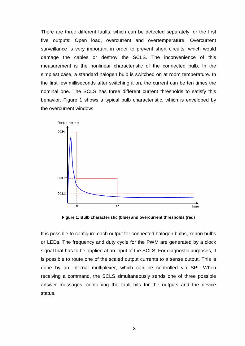
There are three different faults, which can be detected separately for the first

five outputs: Open load, overcurrent and overtemperature. Overcurrent

surveillance is very important in order to prevent short circuits, which would

damage the cables or destroy the SCLS. The inconvenience of this

measurement is the nonlinear characteristic of the connected bulb. In the

simplest case, a standard halogen bulb is switched on at room temperature. In

the first few milliseconds after switching it on, the current can be ten times the

nominal one. The SCLS has three different current thresholds to satisfy this

behavior. Figure 1 shows a typical bulb characteristic, which is enveloped by

the overcurrent window:

Figure 1: Bulb characteristic (blue) and overcurren t thresholds (red)

It is possible to configure each output for connected halogen bulbs, xenon bulbs

or LEDs. The frequency and duty cycle for the PWM are generated by a clock

signal that has to be applied at an input of the SCLS. For diagnostic purposes, it

is possible to route one of the scaled output currents to a sense output. This is

done by an internal multiplexer, which can be controlled via SPI. When

receiving a command, the SCLS simultaneously sends one of three possible

answer messages, containing the fault bits for the outputs and the device

status.

4

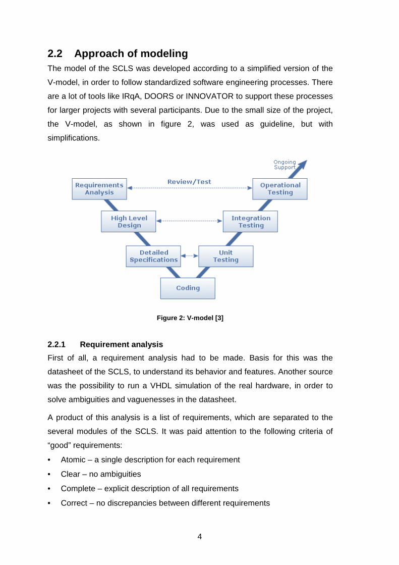
2.2 Approach of modeling The model of the SCLS was developed according to a simplified version of the

V-model, in order to follow standardized software engineering processes. There

are a lot of tools like IRqA, DOORS or INNOVATOR to support these processes

for larger projects with several participants. Due to the small size of the project,

the V-model, as shown in figure 2, was used as guideline, but with

simplifications.

Figure 2: V-model [3]

2.2.1 Requirement analysis

First of all, a requirement analysis had to be made. Basis for this was the

datasheet of the SCLS, to understand its behavior and features. Another source

was the possibility to run a VHDL simulation of the real hardware, in order to

solve ambiguities and vaguenesses in the datasheet.

A product of this analysis is a list of requirements, which are separated to the

several modules of the SCLS. It was paid attention to the following criteria of

“good” requirements:

• Atomic – a single description for each requirement

• Clear – no ambiguities

• Complete – explicit description of all requirements

• Correct – no discrepancies between different requirements

5

• Numbered – a unique identification for each requirement

• Testable – at least one test case per requirement

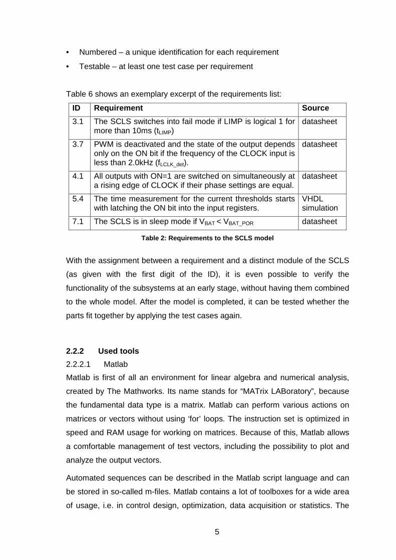
Table 6 shows an exemplary excerpt of the requirements list:

ID Requirement Source

3.1 The SCLS switches into fail mode if LIMP is logical 1 for more than 10ms (tLIMP)

datasheet

3.7 PWM is deactivated and the state of the output depends only on the ON bit if the frequency of the CLOCK input is less than 2.0kHz (fLCLK_det).

datasheet

4.1 All outputs with ON=1 are switched on simultaneously at a rising edge of CLOCK if their phase settings are equal.

datasheet

5.4 The time measurement for the current thresholds starts with latching the ON bit into the input registers.

VHDL simulation

7.1 The SCLS is in sleep mode if VBAT < VBAT_POR datasheet

Table 2: Requirements to the SCLS model

With the assignment between a requirement and a distinct module of the SCLS

(as given with the first digit of the ID), it is even possible to verify the

functionality of the subsystems at an early stage, without having them combined

to the whole model. After the model is completed, it can be tested whether the

parts fit together by applying the test cases again.

2.2.2 Used tools

2.2.2.1 Matlab

Matlab is first of all an environment for linear algebra and numerical analysis,

created by The Mathworks. Its name stands for “MATrix LABoratory”, because

the fundamental data type is a matrix. Matlab can perform various actions on

matrices or vectors without using ‘for’ loops. The instruction set is optimized in

speed and RAM usage for working on matrices. Because of this, Matlab allows

a comfortable management of test vectors, including the possibility to plot and

analyze the output vectors.

Automated sequences can be described in the Matlab script language and can

be stored in so-called m-files. Matlab contains a lot of toolboxes for a wide area

of usage, i.e. in control design, optimization, data acquisition or statistics. The

6

most famous add-on is the Simulink toolbox, which will be described in the

following chapter.

2.2.2.2 Simulink

Matlab is a useful tool for preparing and analyzing test cases, but the modeling

and the simulation are done in Simulink. This toolbox provides a graphical

interface for “visual programming” of the information flow. It consists of a set of

block libraries for various applications, such as for example signal processing,

fuzzy logic or neural networks.

A block is the basic object in Simulink. Its attributes can be configured as

constants or as variables from the Matlab workspace. Several blocks that are

used for one task can be combined to a subsystem that has input and output

ports. Thereby, it is possible to segment a model by building a hierarchy of

subsystems. The Simulink solver is able to work with a variable- or fixed-step

sample time. For discrete systems and code generation it is recommended to

use a fixed sample rate with a discrete solver. Only this allows a sensible

creation of test vectors, because every time step has a defined value.

2.2.2.3 TargetLink

TargetLink is a production-quality code generator created by dSpace, which is

completely integrated in Matlab/Simulink. It mainly consists of special blocks,

similar to the standard Simulink ones, but with additional settings for scaling,

logging and overflow detection. Another important block is the TargetLink Main

Dialog, which offers a lot of adjustments for the code generator. Subsystems

that should be regarded for code generation have to be contained in a special

TargetLink subsystem, which acts as interface to the remaining model in the

different kinds of simulation.

TargetLink works with three different simulation modes:

• In model-in-the-loop (MIL) simulation, all calculations are done by using 64-

bit floating-point variables. The model runs completely in Simulink, without

regarding the scalings. This produces a reference for the following modes. It

is also possible to detect overflows if limitations are correctly set.

7

• After the code generation and build process, it is possible to run a software-

in-the-loop (SIL) simulation. This means that the blocks in the TargetLink

subsystem are replaced by a Simulink s-function, which contains the

generated code. In this mode, all effects of fixed-point arithmetic take place.

The results can be compared with the reference from the MIL simulation in

order to control whether the loss of accuracy can be accepted or not.

• In processor-in-the-loop (PIL) simulation, it is even possible to compile the

code and execute it on an evaluation board that is connected to the

development environment. In addition to the normal logging features, it is

possible to measure the runtime and the stack-size needed.

These features allow that the development of algorithms (often done in

Simulink) and the implementation and coding (normally done by hand) can be

accomplished without changing the toolchain.

2.2.3 Development environment

The model of the SCLS is placed in a development environment for the high-

level driver shown in figure 3. It contains the HLD itself, the SCLS model and

instances of the bulb model for the six outputs.

Figure 3: Development environment for the HLD

inputs

outputs high-level driver

Smart Corner Light Switch

connected loads

8

The green blocks on the left are stimulating the HLD with the test vectors of the

Matlab workspace. They simulate the requests and instructions, which are

normally sent by the application software. Fault bits and sense values are

normally returned to the application. In the development environment, these

values are saved to variables in the workspace. This is done by the red block on

the lower left.

There is one closed loop between HLD that transmits the SPI messages and

SCLS, which feeds back the answers. Another one is between SCLS and the

bulb model, which calculates the current depending on voltage and temperature

and returns these values to the SCLS.

2.2.4 Verification of the SCLS model

The quality of the SCLS model plays a very important role for the development

of the driver, because the model-based approach is only sensible if the modeled

system is free of faults. Otherwise, it could be possible that the driver works

perfectly in the simulation, but not with the real hardware. Therefore, the model

has to take a wide set of tests.

2.2.4.1 Creation of test cases

All developed test cases are directly derived from the list of requirements. It is

documented which test case covers which requirement and vice versa. A test

case describes the principle procedure of the test. These are the test steps and

the expected results.

The real SCLS is tested with an automatic test rack. Some test cases are

adopted from this automatic test specification, in order to have a possibility to

compare between simulation and reality.

2.2.4.2 Explanation of the test environment

Matlab and Simulink are of course not able to work with this description in

natural language. Therefore, every test case has to be converted into test

vectors that have a defined value for each time step and for each input. For the

9

decision whether a test was correct or has failed, it is important to have vectors

with the expected output values, too. Since the SCLS model has 42 inputs and

37 outputs, it is hard not to loose the overview.

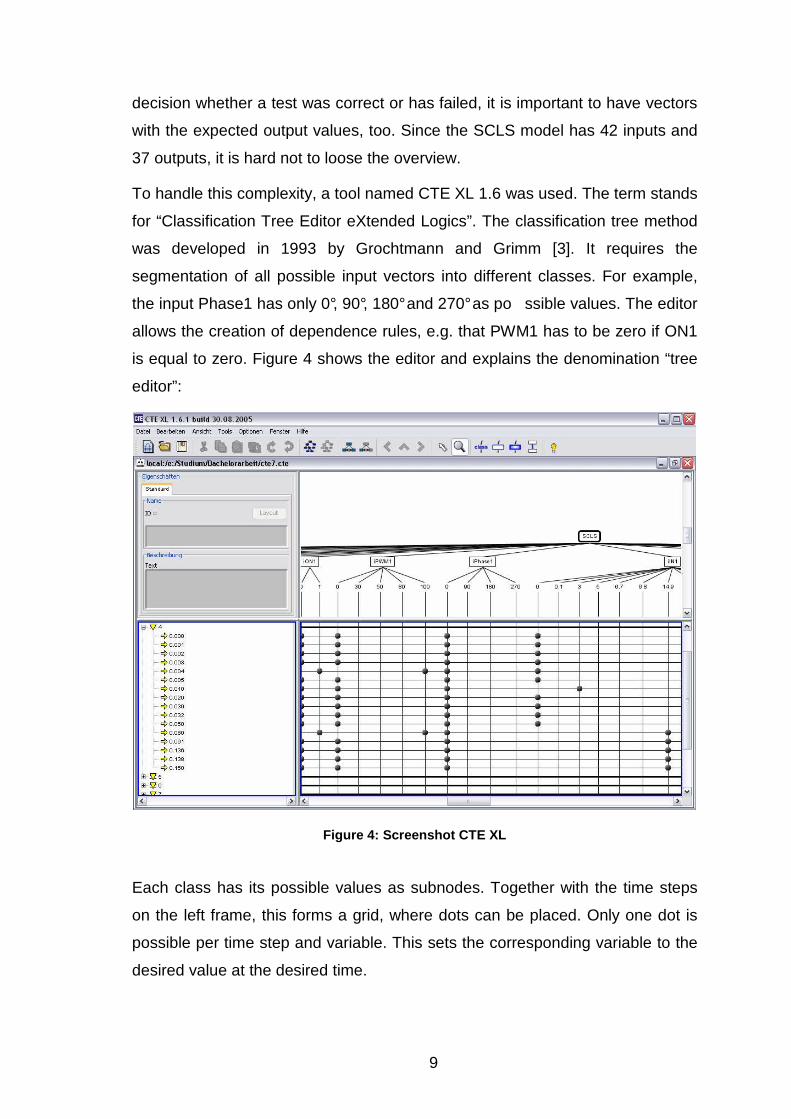
To handle this complexity, a tool named CTE XL 1.6 was used. The term stands

for “Classification Tree Editor eXtended Logics”. The classification tree method

was developed in 1993 by Grochtmann and Grimm [3]. It requires the

segmentation of all possible input vectors into different classes. For example,

the input Phase1 has only 0°, 90°, 180° and 270° as po ssible values. The editor

allows the creation of dependence rules, e.g. that PWM1 has to be zero if ON1

is equal to zero. Figure 4 shows the editor and explains the denomination “tree

editor”:

Figure 4: Screenshot CTE XL

Each class has its possible values as subnodes. Together with the time steps

on the left frame, this forms a grid, where dots can be placed. Only one dot is

possible per time step and variable. This sets the corresponding variable to the

desired value at the desired time.

10

CTE XL allows the export of data to many different file formats. The export to

Matlab generates an m-file that creates a structure in the Matlab workspace.

This structure can be analyzed and segmented to the different test vectors with

the help of a simple script.

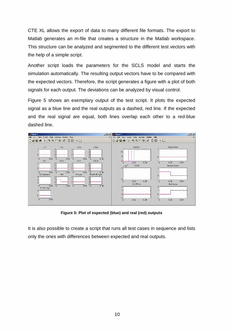
Another script loads the parameters for the SCLS model and starts the

simulation automatically. The resulting output vectors have to be compared with

the expected vectors. Therefore, the script generates a figure with a plot of both

signals for each output. The deviations can be analyzed by visual control.

Figure 5 shows an exemplary output of the test script. It plots the expected

signal as a blue line and the real outputs as a dashed, red line. If the expected

and the real signal are equal, both lines overlap each other to a red-blue

dashed line.

Figure 5: Plot of expected (blue) and real (red) ou tputs

It is also possible to create a script that runs all test cases in sequence and lists

only the ones with differences between expected and real outputs.

11

3 Explanation of the bulb model 3.1 Reasons for using a bulb model Normally, a bulb is regarded as a simple resistor, which is true as a first

approximation. Its filament is made up of metal (tungsten) and Ohm’s law is

valid. But on closer examination, it can be seen that its resistance is not

constant, but depends on the temperature. Halogen lamps heat up to about

2700K [4], which causes a huge difference between the resistance at room

temperature and operating temperature. The effect to the current through the

bulb is shown in figure 1. It can rise to about ten times the nominal current

shortly after switching on the voltage. This is quite normal and must not be

treated as short circuit. To validate the behavior of the software in this case, all

tests in the development of body controllers are done with original loads and not

with ohmic resistors.

For the modeling in Simulink, these original loads have to be replaced by a bulb

model. This offers a wider range of feasible tests. For example, it is possible to

simulate the switching of a lamp at an ambient temperature of -40°C – simply by

changing a parameter.

Another decisive factor for the current curve is the duty cycle. If a bulb is driven

with a very low duty cycle at low temperature, it might perhaps not heat up fast

enough to have a current, which is below the third overcurrent threshold

(OCLO). The ECU software has to avoid that by heating the bulb with higher

duty cycle in the first milliseconds and setting the lower duty cycle afterward.

The model of the SCLS needs a feedback of the output current, because it only

computes the voltage and the current depends on the connected load. Of

course, the values of the current inputs can be defined in the test vectors. But it

is easier and closer to reality if the values are calculated by a bulb model. Real

short circuit and open load conditions can thereby be simulated by routing back

either the bulb current, no current or an extremely high current.

This method of reconnecting the outputs to the inputs is called closed-loop

simulation, because the feedback is done in the model itself and is not

determined by external input vectors.

12

3.2 Physical basics Behind the bulb model are a few formulas of thermodynamics and electrical

engineering. They are based on three simplifications:

(1) All electrical energy is converted to heat. Normally, about 5% of the whole

energy is emitted as light.

(2) There is no additional heating by the other bulbs in the headlights. All heat

comes from the own electrical power.

(3) The only mass that is heated up is the tungsten filament in the lamp. It is

assumed that the proximate environment (e.g. the glass of the bulb) is not

heated up.

The aim of the calculations is to get a current depending on voltage,

temperature and time. First of all, current depends on voltage and resistance

according to Ohm’s law:

R

UI = (3.1)

The resistance of a metal varies with changing temperature as shown in the

following equation where R20 is the resistance at 20°C and α is the temperature

coefficient of the material. The temperature of the filament in °C is the

variableϑ .

( )[ ]CRR °−⋅+⋅= 20120 ϑα (3.2)

By considering the different forms of energy, it is possible to get a correlation

between power and temperature. According to the first law of thermodynamics,

the energy flowing into a system is equal to the sum of the increase in the

internal energy of the system and the work done by the system. This is valid

under consideration of simplifications (1) and (2) and leads to equation (3.3):

outheatel QQW += (3.3)

13

The electrical energy in a resistive load is determined by voltage, current and

time:

tIUtPW elel ⋅⋅=⋅= (3.4)

The increase of internal energy, which heats the filament, can be described as

follows:

TcmQheat ∆⋅⋅= (3.5)

Variables of this equation are the mass m of the filament, the specific heat

capacity c of tungsten and the difference ∆T between the initial temperature and

the temperature of the hot filament.

A part of the energy is emitted as heat. Its magnitude depends on the thermal

resistance Rth between bulb and ambience. Since the initial temperature of the

filament is equal to the ambient temperature, ∆T in equation (3.5) is the same

as in equation (3.6).

tR

TQ

thout ⋅∆= (3.6)

Applying this to equation (3.3) leads to:

tR

TTcmtP

thel ⋅∆+∆⋅⋅=⋅ (3.7)

It is possible to get a first-order differential equation after division by an infinitely

small time step ∆t:

TR

Tdt

dcmP

thel ∆⋅+∆⋅⋅= 1

(3.8)

14

By application of the Laplace transform and setting all initial conditions to zero,

a transfer function can be set up:

thRscm

sH1

1

PL

TL)(

el +⋅⋅=∆= (3.9)

Since the simulation is a discrete system, a Z-transform of this continuous

function has to be used. This can for example be done with the Tustin

approximation (also called bilinear transform):

1

12

+−⋅=

z

z

Ts

sample (3.10)

Inserting this in equation (3.9) leads to the final discrete transfer function used

in the bulb model:

( )

⋅⋅−+

⋅⋅+⋅

+=

samplethsampleth T

cm

RT

cm

Rz

zzH

2121

1 (3.11)

Since it is known that the temperature of the filament is approximately 2700K in

steady state [4], it is possible to determine the thermal resistance. This can be

calculated by setting the derivative of the temperature difference ∆T in equation

(3.8) to zero, which leads to the following formula:

W

K

W

K

P

TR

elth 50

55

2700 ≈=∆= (3.12)

The following list gives an overview of the used constants:

Temperature coefficient of tungsten: K

1108.4 3−⋅=α [5]

Specific heat capacity of tungsten: Kkg

Jc

⋅= 143 [5]

Mass of the filament: mgm 35≈ (estimated)

15

Thermal resistance (bulb to ambience): W

KRth 50≈ (calculated)

R20 of a 55W halogen bulb (H7): Ω≈ 24.020R (measured)

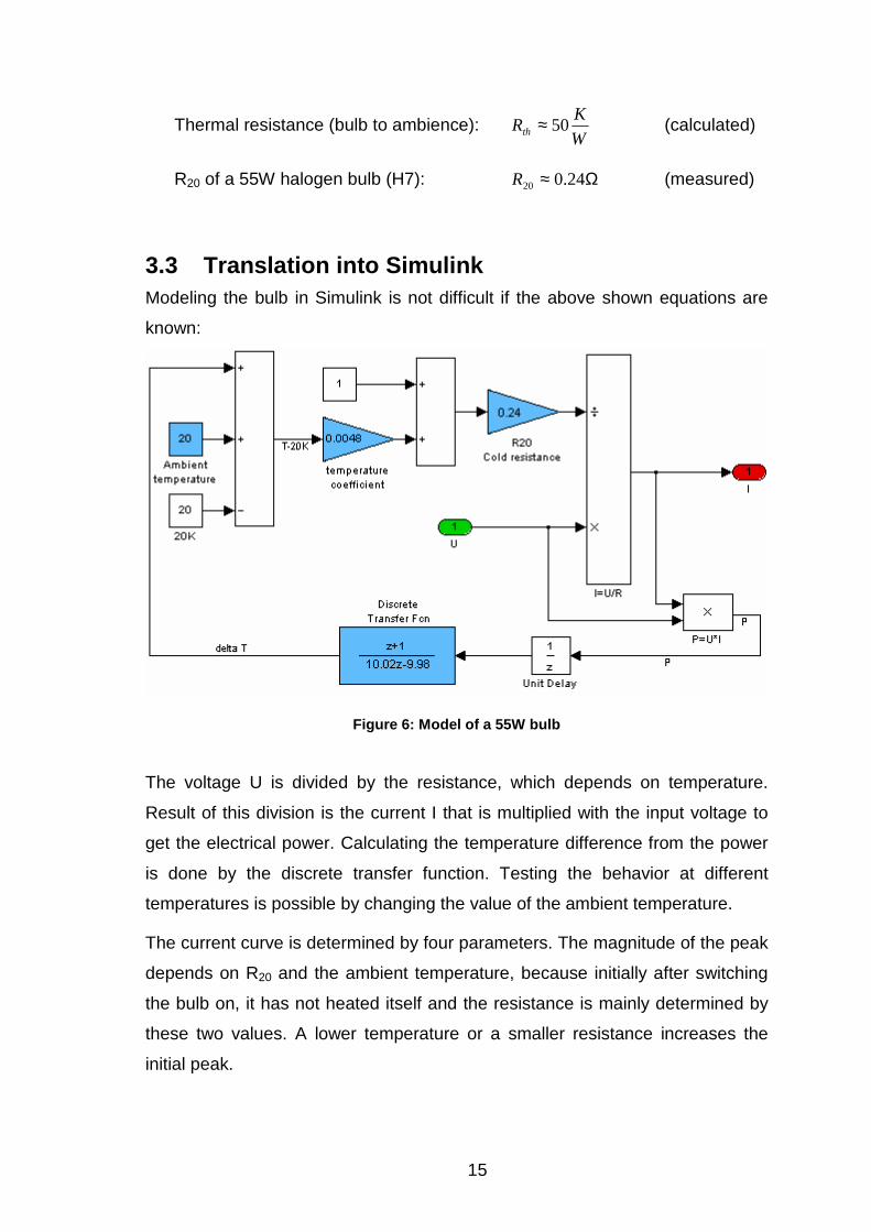
3.3 Translation into Simulink Modeling the bulb in Simulink is not difficult if the above shown equations are

known:

Figure 6: Model of a 55W bulb

The voltage U is divided by the resistance, which depends on temperature.

Result of this division is the current I that is multiplied with the input voltage to

get the electrical power. Calculating the temperature difference from the power

is done by the discrete transfer function. Testing the behavior at different

temperatures is possible by changing the value of the ambient temperature.

The current curve is determined by four parameters. The magnitude of the peak

depends on R20 and the ambient temperature, because initially after switching

the bulb on, it has not heated itself and the resistance is mainly determined by

these two values. A lower temperature or a smaller resistance increases the

initial peak.

16

Decisive for the time, until a steady state is reached, is the value of sampleT

cm ⋅⋅2 in

the transfer function. A higher mass extends this time, because more energy is

necessary to get the same operating temperature. The used value of 10J/Ks

with a sample time of 0.001s leads to a mass of the filament of 35mg. This

estimated value is confirmed by the technical support of the bulb manufacturer

OSRAM. Typical values for the filament’s mass in halogen bulbs are between

23mg and 35mg.

If the steady state is reached, the derivation of the temperature in equation (3.8)

becomes zero. This causes a linear correlation between electrical power and

temperature, determined by the thermal resistance Rth as described in equation

(3.12). The model uses a value of 50K/W. Increasing it leads to less current in

steady state, because the temperature (and thus the electrical resistance) rises,

since the transfer of heat is hampered.

Knowing the effects of these parameters allows testing the SCLS driver e.g.

with bulbs that need a longer time to reach the steady state.

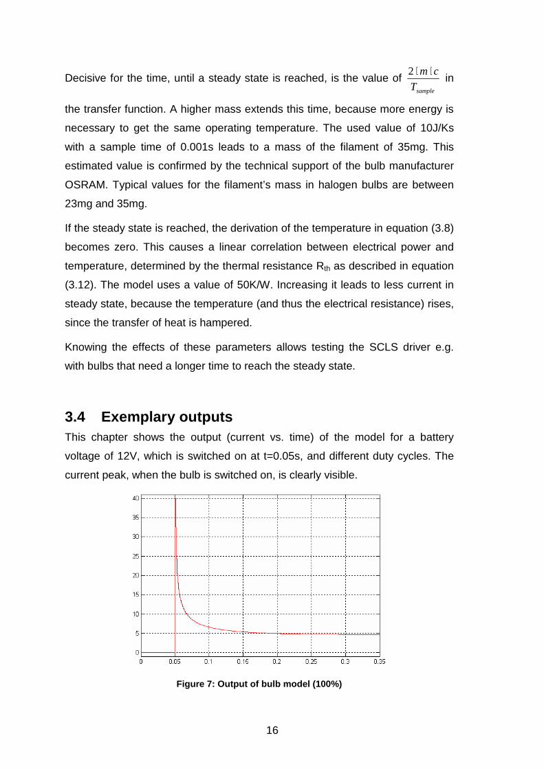
3.4 Exemplary outputs This chapter shows the output (current vs. time) of the model for a battery

voltage of 12V, which is switched on at t=0.05s, and different duty cycles. The

current peak, when the bulb is switched on, is clearly visible.

Figure 7: Output of bulb model (100%)

17

If the voltage is pulse width modulated, the filament cools down in the off-time of

PWM. This can be seen in figure 8, where the current at the beginning of one

pulse is higher than at the end of the pulse before, if the temperature has

reached its operational value.

Figure 8: Output of bulb model (50%)

More detailed diagrams and a comparison to real bulb currents are given in

chapter 5.

4 Driver description 4.1 Task system Controlling the SCLS requires four functions that have to be called in defined

time intervals:

• The high-level driver itself, which prepares the data to send.

• The SPI driver, which manages the transmission to e.g. four Corner Light

ICs by using daisy chain.

• The AD converter that reads the current sense value.

• The application, which controls the HLD.

The SPI driver can not be called from the HLD, because the HLD function is

only written to control one device. In contrast, the SPI driver has to wait until all

four HLDs have set up their commands. Since the SCLS resets its fault

18

registers after sending their content to the microcontroller, and buffering the

data requires a lot of memory, it was determined to call the SPI driver exactly

once between two calls of the HLDs. Hence, a loss of data is avoided.

This method even works in an OSEK system, if both functions are invoked in

one task. The application and the AD conversion run independent of the drivers.

Realistic values are an interval of 5ms between the driver calls and an

execution of the application every 20ms. Timing of the AD conversion depends

on the sampling method.

Another problem is multiplexing the current sense. To save the few AD

channels of the microcontroller, all current sense outputs are connected to the

same pin of the microcontroller. Therefore, it has to be ensured that only one

SCLS delivers its sense current at any given time. Since the HLD function is

only an instance that doesn’t know about the other ones, a superior logic is

necessary to determine, which instance is able to route one of its outputs to the

processor.

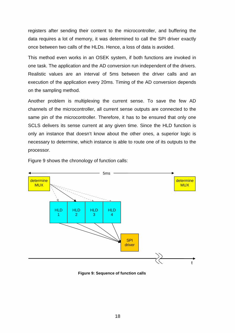
Figure 9 shows the chronology of function calls:

Figure 9: Sequence of function calls

HLD

1

HLD

2

HLD

3

HLD

4

SPI driver

determine MUX

determine MUX

5ms

t

19

4.2 Initialization and reset After switching on its supply voltage, the SCLS needs a defined initialization

procedure:

• Waking the device by setting the reset pin (RSTB) to high level and applying

the clock signal.

• Sending an initialization message with WD=1 to trigger the watchdog and

SOA=2 to clear an eventually set Clock-fail flag. This message also contains

the XenonB bit.

• Sending a message to configure the outputs as LED or bulb.

Since the driver has outputs for RSTB, Clock and message address that are

only calculated once in one step, it is not possible to change them frequently

within one function call. For example, the SIA can only have exactly one value

in each simulation step, because it is only one output of the model. It is not

possible to assign SIA=0 (Initialization message) and SIA=1 (Config OL

message) in one function call. Thus, the driver needs to be called three times to

perform the complete initialization procedure.

If the microcontroller switches into sleep mode, the SCLS has to sleep, too.

Otherwise it would recognize fail mode (because the SPI watchdog is no longer

triggered) and activate the emergency light. Therefore, the driver has to take

care that the RSTB pin is pulled to low level in this case.

To satisfy these requirements, the driver provides two inputs, called

AppActivateSCLS and AppResetSCLS. The former named is the more

important. If it is zero, the SCLS is set to sleep mode. A transition from zero to

one starts the initialization. As long as it does not return to zero, the driver is

ready for use. This is accomplished by holding a state counter that is increased

in each initialization step and remains constant if the normal operational mode

is reached. If using just the activateSCLS bit, the application can perform a

reset of the SCLS (e.g. after detecting a fault) only by resetting it to zero and

increasing it to one in the next cycle, which would be approximately 20ms later.

This is the typical use case for the resetSCLS bit: Setting it to one resets the

state counter and thereby the SCLS. Thus, the re-initialization of the device can

20

start with the next call of the HLD, i.e. 5ms later. In this case, activateSCLS

stays at logical one for the whole time and resetSCLS is set back to zero within

the following execution of the application. Since the integrator is only reset after

a positive edge, it is no problem that the value of resetSCLS remains one until

the next application call.

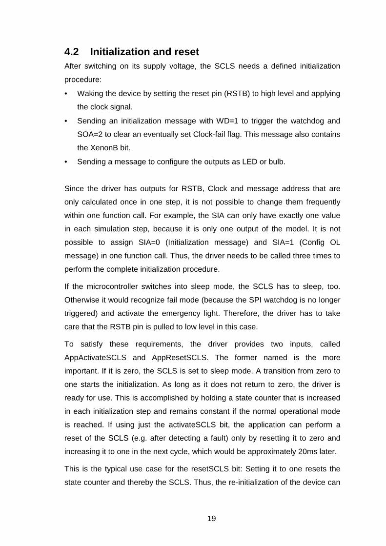
Figure 10: State machine

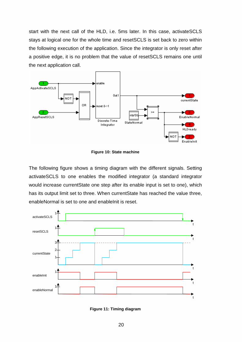
The following figure shows a timing diagram with the different signals. Setting

activateSCLS to one enables the modified integrator (a standard integrator

would increase currentState one step after its enable input is set to one), which

has its output limit set to three. When currentState has reached the value three,

enableNormal is set to one and enableInit is reset.

Figure 11: Timing diagram

t

t

t

t

t

activateSCLS

resetSCLS

currentState

enableNormal

enableInit 1

3

1

1

1

1

2

21

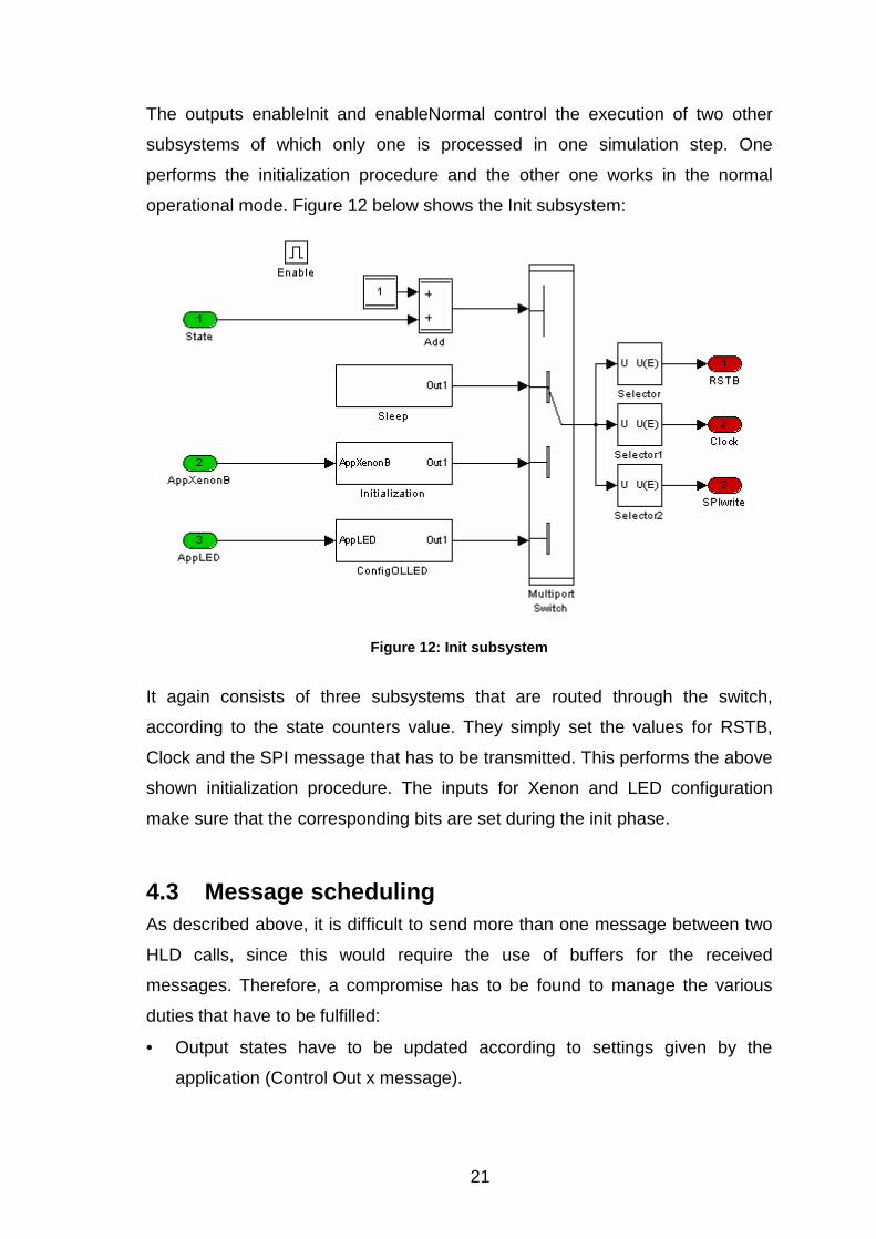
The outputs enableInit and enableNormal control the execution of two other

subsystems of which only one is processed in one simulation step. One

performs the initialization procedure and the other one works in the normal

operational mode. Figure 12 below shows the Init subsystem:

Figure 12: Init subsystem

It again consists of three subsystems that are routed through the switch,

according to the state counters value. They simply set the values for RSTB,

Clock and the SPI message that has to be transmitted. This performs the above

shown initialization procedure. The inputs for Xenon and LED configuration

make sure that the corresponding bits are set during the init phase.

4.3 Message scheduling As described above, it is difficult to send more than one message between two

HLD calls, since this would require the use of buffers for the received

messages. Therefore, a compromise has to be found to manage the various

duties that have to be fulfilled:

• Output states have to be updated according to settings given by the

application (Control Out x message).

22

• Alternating requests for the three different answer messages have to be

made (Initiaization message).

• The channel of the internal multiplexer must be changed after a time that

was long enough to sample the complete signal of one output (Initialization

message).

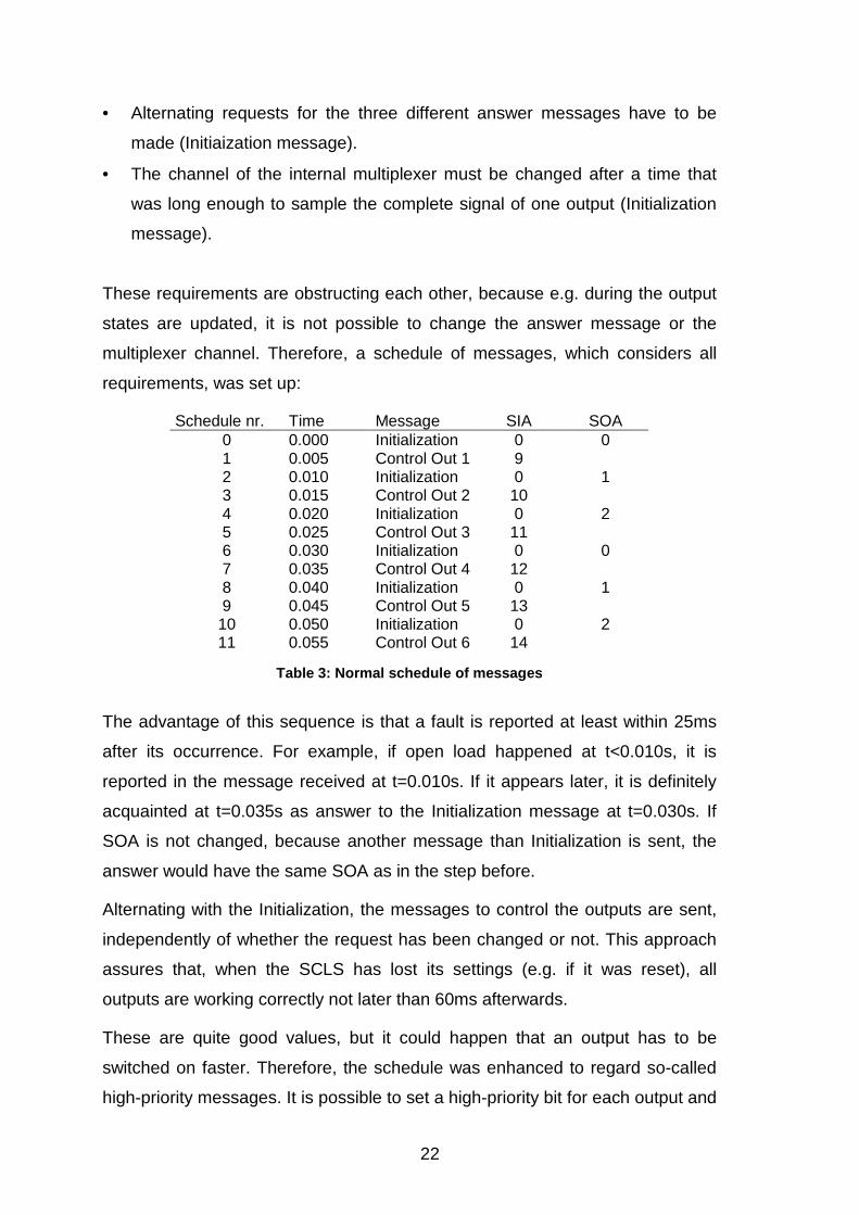
These requirements are obstructing each other, because e.g. during the output

states are updated, it is not possible to change the answer message or the

multiplexer channel. Therefore, a schedule of messages, which considers all

requirements, was set up:

Schedule nr. Time Message SIA SOA 0 0.000 Initialization 0 0 1 0.005 Control Out 1 9 2 0.010 Initialization 0 1 3 0.015 Control Out 2 10 4 0.020 Initialization 0 2 5 0.025 Control Out 3 11 6 0.030 Initialization 0 0 7 0.035 Control Out 4 12 8 0.040 Initialization 0 1 9 0.045 Control Out 5 13 10 0.050 Initialization 0 2 11 0.055 Control Out 6 14

Table 3: Normal schedule of messages

The advantage of this sequence is that a fault is reported at least within 25ms

after its occurrence. For example, if open load happened at t<0.010s, it is

reported in the message received at t=0.010s. If it appears later, it is definitely

acquainted at t=0.035s as answer to the Initialization message at t=0.030s. If

SOA is not changed, because another message than Initialization is sent, the

answer would have the same SOA as in the step before.

Alternating with the Initialization, the messages to control the outputs are sent,

independently of whether the request has been changed or not. This approach

assures that, when the SCLS has lost its settings (e.g. if it was reset), all

outputs are working correctly not later than 60ms afterwards.

These are quite good values, but it could happen that an output has to be

switched on faster. Therefore, the schedule was enhanced to regard so-called

high-priority messages. It is possible to set a high-priority bit for each output and

23

for Initialization, which discontinues the normal sequence to send a distinct

message.

To prevent the other messages from starving out, only three high-priority

messages can be sent between two regular Initialization messages. Three

conditions need to be fulfilled, to interrupt the schedule: The high-priority bit of a

message is set, less than two high-priority messages were sent since the last

regular Initialization message and the settings of the addressed output have to

be unequal to those already sent.

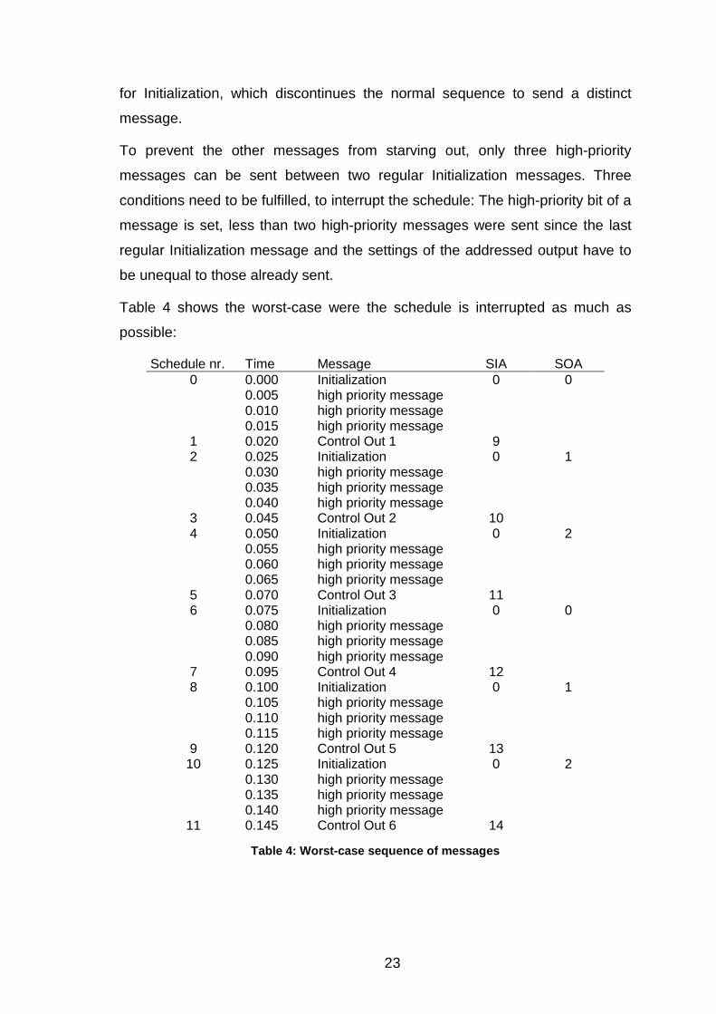
Table 4 shows the worst-case were the schedule is interrupted as much as

possible:

Schedule nr. Time Message SIA SOA 0 0.000 Initialization 0 0 0.005 high priority message 0.010 high priority message 0.015 high priority message 1 0.020 Control Out 1 9 2 0.025 Initialization 0 1 0.030 high priority message 0.035 high priority message 0.040 high priority message 3 0.045 Control Out 2 10 4 0.050 Initialization 0 2 0.055 high priority message 0.060 high priority message 0.065 high priority message 5 0.070 Control Out 3 11 6 0.075 Initialization 0 0 0.080 high priority message 0.085 high priority message 0.090 high priority message 7 0.095 Control Out 4 12 8 0.100 Initialization 0 1 0.105 high priority message 0.110 high priority message 0.115 high priority message 9 0.120 Control Out 5 13

10 0.125 Initialization 0 2 0.130 high priority message 0.135 high priority message 0.140 high priority message

11 0.145 Control Out 6 14

Table 4: Worst-case sequence of messages

24

This could only happen if the settings for the duty cycles are changed in every

application call. Considering the timing, it is shown that a fault is acquainted at

the latest after 55ms. This is short enough for diagnosis, because the main

protection is done in the SCLS. The time after which all outputs are surely

updated is 150ms. Through the possibility to set the high-priority bits for more

time-critical outputs, this should be short enough, too.

There is no explicit high-priority bit for the ‘Config OL’ message, because it is

internally set to one. Since this message does not appear in the schedule, LED

configuration is always handled as high prioritized task.

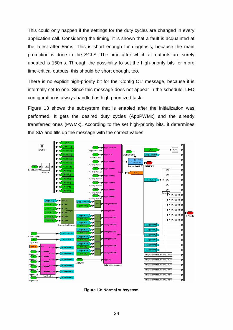
Figure 13 shows the subsystem that is enabled after the initialization was

performed. It gets the desired duty cycles (AppPWMx) and the already

transferred ones (PWMx). According to the set high-priority bits, it determines

the SIA and fills up the message with the correct values.

Figure 13: Normal subsystem

25

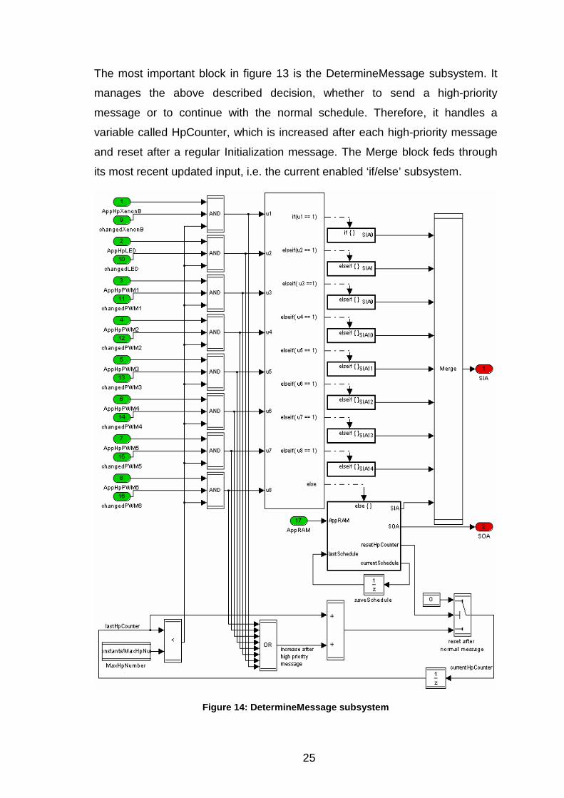
The most important block in figure 13 is the DetermineMessage subsystem. It

manages the above described decision, whether to send a high-priority

message or to continue with the normal schedule. Therefore, it handles a

variable called HpCounter, which is increased after each high-priority message

and reset after a regular Initialization message. The Merge block feds through

its most recent updated input, i.e. the current enabled ‘if/else’ subsystem.

Figure 14: DetermineMessage subsystem

26

If there are more high-priority messages at the same time, the order of

execution is defined by the positions in the ‘If’ subsystem. Anyway, only one

message per simulation step is possible and the others have to wait until the

next step (perhaps even until the next regular Initialization message was sent).

The ‘If’ block enables the first subsystem, whose condition is true. All the other

blocks are then disabled in this step, even if their condition is fulfilled, too. For

example, if the inputs ‘u2’ and ‘u5’ are both logical true, the ‘elseif’ block for ‘u2’

will be enabled first.

In theory, it is possible that some lower positioned messages will never be

transferred. But this could only happen if there are more messages with

permanentely changing values. This case is very unlikely and if it happens

nevertheless, the corresponding output will be at least updated within the

regular schedule. This is guaranteed by the schedule, shown in table 4, where

every message is sent at least once within 150ms, even in worst-case.

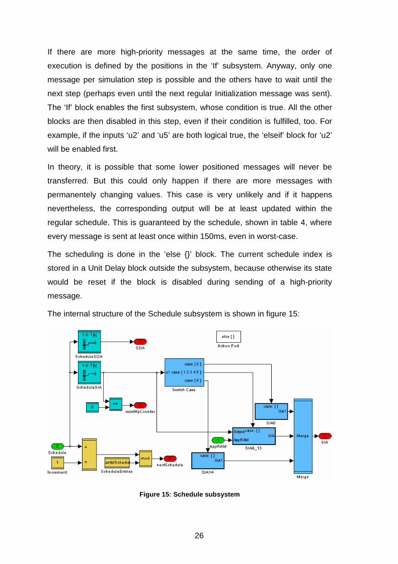
The scheduling is done in the ‘else ’ block. The current schedule index is

stored in a Unit Delay block outside the subsystem, because otherwise its state

would be reset if the block is disabled during sending of a high-priority

message.

The internal structure of the Schedule subsystem is shown in figure 15:

Figure 15: Schedule subsystem

27

It is mainly divided into three parts. The yellow part on the lower left increases

the index of the schedule and resets it when the maximum value is reached.

The green part determines the current SIA and SOA, according to the schedule

index. Furthermore, it decides whether the high-priority counter should be reset.

To do this, it uses discrete look-up tables. A normal Simulink look-up table

would cause a huge overhead in the generated code, because special search

and interpolation functions will be inserted, although they are not needed for

these integer variables. A discrete look-up table, in contrast, generates an

array, which is accessed by the schedule index.

Another way could be the calculation of SIA and SOA out of the index by using

integer divisions and modulo operations. This would decrease the amount of

ROM needed, since the entries of the tables need not to be stored. A

disadvantage is, modifying the schedule would cause a complete exchange of

the calculation procedures. Therefore, the usage of the look-up table was

considered to be more comfortable.

A reset of the HpCounter is performed after a regular Initialization message

(SIA=0).

The blue part on the right side of figure 15 avoids retries on outputs that were

shut down. Therefore, it eventually replaces the calculated SIA.

28

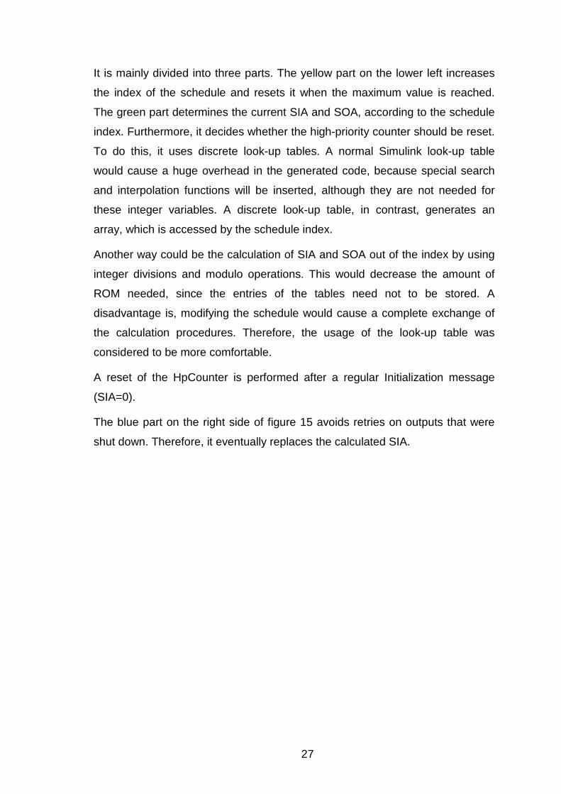
5 Hardware-in-the-loop tests with CANoe 5.1 Reasons for HIL tests Until now, all tests were accomplished by using models of the real hardware. In

order to eliminate failures in the models, it is useful to test the developed

system with real hardware, too. In the present test environment, the SCLS and

the bulbs are simulated. Therefore, it would be the optimal way to test the HLD

with a real SCLS and a real bulb by setting the border between HLD and SCLS

as shown below.

Figure 16: Method 1 for HIL tests

This would mean that the Simulink model has to control the SCLS via a real SPI

interface between PC and SCLS. The interface needs to be able to transmit the

data and receive the answer simultaneously within one simulation step. One

possible solution, which exists at Continental Temic, is a microcontroller board

that is connected to the PC via USB. Furthermore, it has an SPI interface to

control an SCLS. This means that a message would have to be transferred first

of all via USB and then via SPI. After that, the answer would have to be

returned in reverse order.

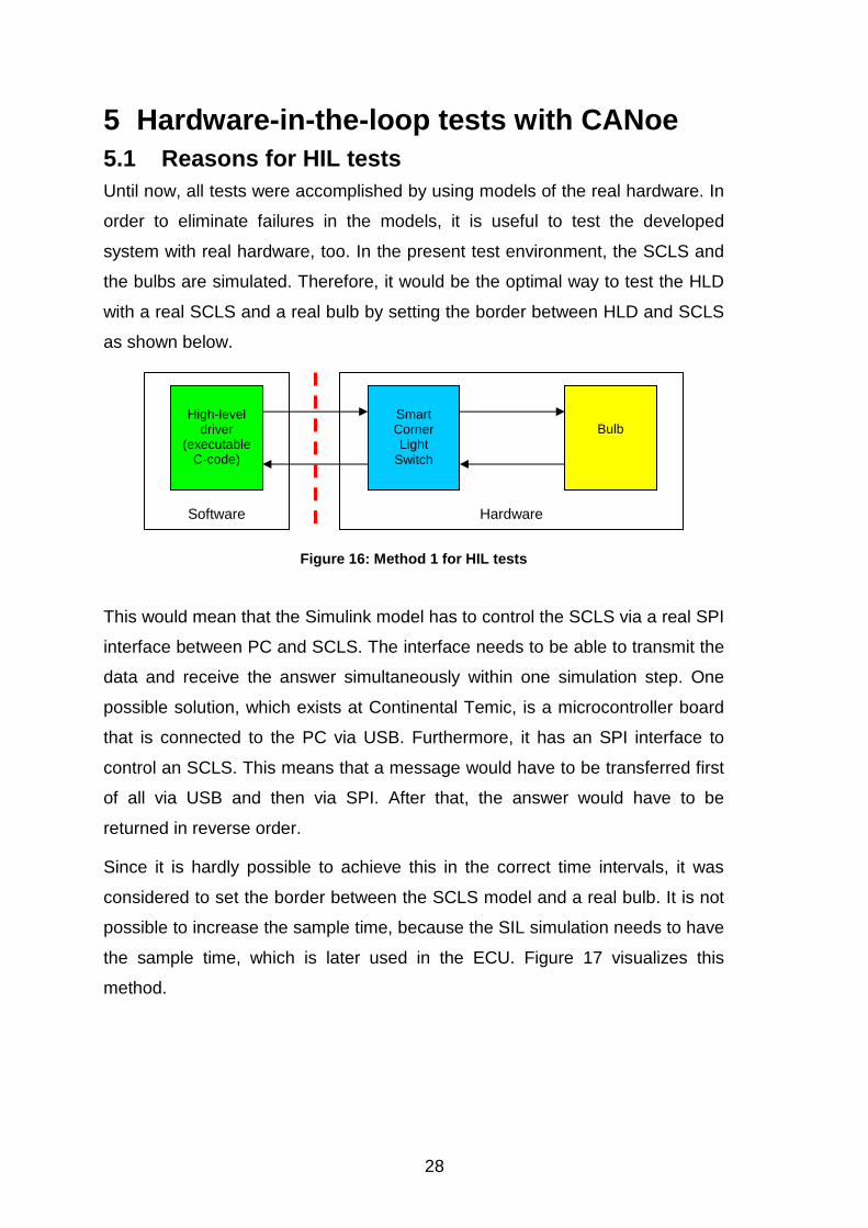
Since it is hardly possible to achieve this in the correct time intervals, it was

considered to set the border between the SCLS model and a real bulb. It is not

possible to increase the sample time, because the SIL simulation needs to have

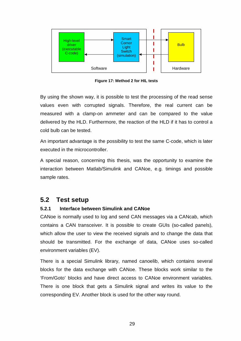
the sample time, which is later used in the ECU. Figure 17 visualizes this

method.

Software

High-level

driver (executable

C-code)

Smart Corner Light

Switch

Bulb

Hardware

29

Figure 17: Method 2 for HIL tests

By using the shown way, it is possible to test the processing of the read sense

values even with corrupted signals. Therefore, the real current can be

measured with a clamp-on ammeter and can be compared to the value

delivered by the HLD. Furthermore, the reaction of the HLD if it has to control a

cold bulb can be tested.

An important advantage is the possibility to test the same C-code, which is later

executed in the microcontroller.

A special reason, concerning this thesis, was the opportunity to examine the

interaction between Matlab/Simulink and CANoe, e.g. timings and possible

sample rates.

5.2 Test setup 5.2.1 Interface between Simulink and CANoe

CANoe is normally used to log and send CAN messages via a CANcab, which

contains a CAN transceiver. It is possible to create GUIs (so-called panels),

which allow the user to view the received signals and to change the data that

should be transmitted. For the exchange of data, CANoe uses so-called

environment variables (EV).

There is a special Simulink library, named canoelib, which contains several

blocks for the data exchange with CANoe. These blocks work similar to the

‘From/Goto’ blocks and have direct access to CANoe environment variables.

There is one block that gets a Simulink signal and writes its value to the

corresponding EV. Another block is used for the other way round.

Software

High-level

driver (executable

C-code)

Smart Corner Light

Switch (simulation)

Bulb

Hardware

30

5.2.2 Interface between CANoe and IOcab

Instead of the CANcab, it is possible to use an IOcab, which has several digital

and analog in-/outputs. This device is controlled via environment variables, too.

The IOcab contains:

• 8 digital inputs or 4 digital outputs (two ports are combined to one output)

• 4 analog inputs or outputs (each port’s direction is configurable)

• a PWM module or a capture/compare unit

It is configured in the Port Link Configuration menu of CANoe. The mapping

between the EVs and the ports has to be done there, too. To control the PWM

and CAPCOM module, two EVs are needed: One for frequency and the other

one for duty cycle. The frequency is set to a constant value, while the duty cycle

depends on the current state of the SCLS.

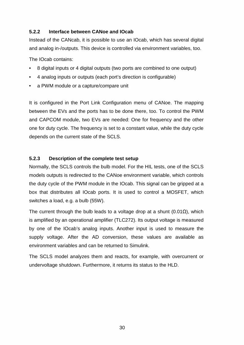
5.2.3 Description of the complete test setup

Normally, the SCLS controls the bulb model. For the HIL tests, one of the SCLS

models outputs is redirected to the CANoe environment variable, which controls

the duty cycle of the PWM module in the IOcab. This signal can be gripped at a

box that distributes all IOcab ports. It is used to control a MOSFET, which

switches a load, e.g. a bulb (55W).

The current through the bulb leads to a voltage drop at a shunt (0.01Ω), which

is amplified by an operational amplifier (TLC272). Its output voltage is measured

by one of the IOcab’s analog inputs. Another input is used to measure the

supply voltage. After the AD conversion, these values are available as

environment variables and can be returned to Simulink.

The SCLS model analyzes them and reacts, for example, with overcurrent or

undervoltage shutdown. Furthermore, it returns its status to the HLD.

31

Figure 18: HIL test setup

In TargetLink, the simulation mode of the HLD is set to SIL. This means that this

setup can test how the real C-code of the HLD works with real loads in real-

time, including all possible fixed-point faults and quantization errors. The

calculation of the SCLS model is done in floating-point arithmetic, since it is still

a normal Simulink subsystem.

The real-time behavior can be achieved by inserting a ‘real-time’ block of an

additional library named rtlib. This increases the priority of the Simulink process

in Windows. It is even possible to connect digital inputs of the IOcab to the

LIMP, FLASHER and IGN inputs of the SCLS. This allows activating fail mode

and switching on emergency light.

Figure 19 shows the real test setup at the workstation. The oscilloscope is used

to compare the real voltages to those returned from CANoe. Since the power

supply is not capable to deliver more than 50A, a battery was connected in

parallel, in order to buffer the current in the moment of switching the bulb on.

32

Between laptop and oscilloscope, the IOcab and the box, which distributes its

signals, can be seen.

Figure 19: Real HIL test setup

Both, distribution box and power module were built up at Continental Temic.

The power module, where the bulb is connected to, is shown in detail in figure

20. It was designed specially for these HIL tests and contains two amplifier

circuits, in order to deliver the current in two different measuring ranges. Since

the analog inputs are capable to measure voltages up to 8V and the typical

currents were estimated to be about 70A (when switching the bulb on) and 5A

(in normal operational mode), it was considered to have one range from 0A to

8A and another one from 0A to 80A.

By removing the bridge between bulb and shunt, it is possible to simulate open

load or to connect e.g. a LED or an electronic load.

Figure 20: Power module for HIL tests

distribution box

IOcab

power module

33

5.3 Test results 5.3.1 Accuracy of the current measurement

First of all, it is important that the current is measured correctly. To verify this, a

clamp-on ammeter was used to get a reference, to which the results of the

shunt measurement can be compared.

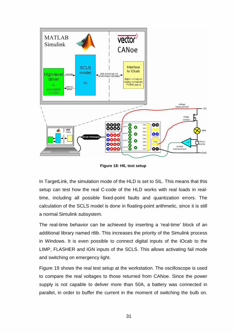
The clamp-on ammeter was inserted at the bridge between bulb and shunt and

connected to channel 4 of the oscilloscope. The voltage at the amplifier with the

higher range was measured at channel 1. Results can be seen in the figure

below, where the left plot shows the current at 100% duty cycle and the right

one at 50%.

Figure 21: Comparison between shunt (ch. 1) and cla mp-on ammeter (ch. 4)

It can be seen that both channels approximately show the same curve. The

peaks in the right picture are supposedly caused by the operational amplifier,

but can be neglected, since they are too short to be acquired by the ADC.

Unfortunately, the IOcab works very inexactly in this frequency range. To get

the above shown frequency of about 100Hz, the corresponding environment

variable has to be set to 140Hz. Even with this value, the frequency dithers

between 90Hz and 110Hz.

The next possible source of error is the AD conversion in the IOcab. Therefore,

its results have to be compared with the real current, as shown in figure 22. The

course of both signals is nearly the same. Only the peak value differs from

54.2A (real) to about 46A (measured by IOcab). This is due to the sampling

frequency of the IOcab, which is 3kHz. This makes a period of more than

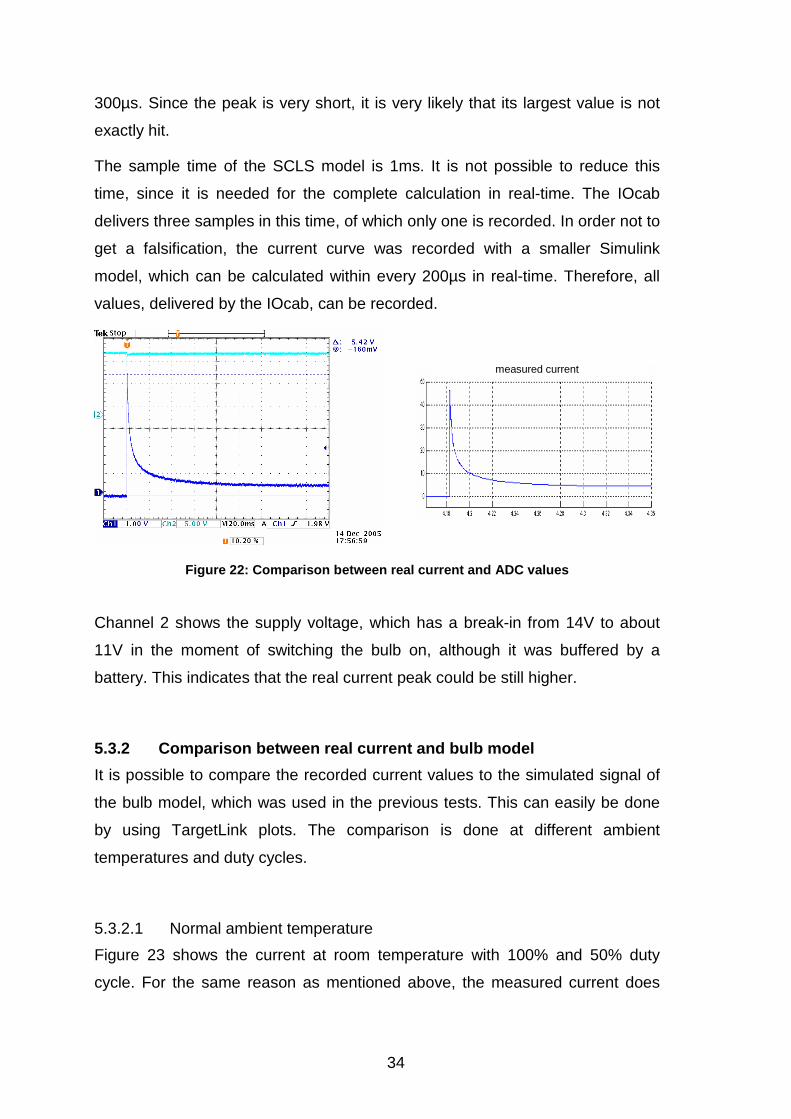
34

300µs. Since the peak is very short, it is very likely that its largest value is not

exactly hit.

The sample time of the SCLS model is 1ms. It is not possible to reduce this

time, since it is needed for the complete calculation in real-time. The IOcab

delivers three samples in this time, of which only one is recorded. In order not to

get a falsification, the current curve was recorded with a smaller Simulink

model, which can be calculated within every 200µs in real-time. Therefore, all

values, delivered by the IOcab, can be recorded.

Figure 22: Comparison between real current and ADC values

Channel 2 shows the supply voltage, which has a break-in from 14V to about

11V in the moment of switching the bulb on, although it was buffered by a

battery. This indicates that the real current peak could be still higher.

5.3.2 Comparison between real current and bulb mode l

It is possible to compare the recorded current values to the simulated signal of

the bulb model, which was used in the previous tests. This can easily be done

by using TargetLink plots. The comparison is done at different ambient

temperatures and duty cycles.

5.3.2.1 Normal ambient temperature

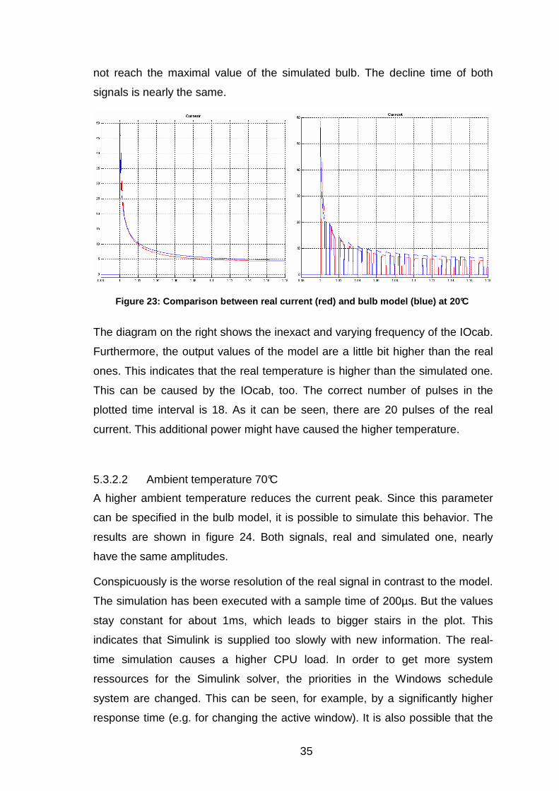
Figure 23 shows the current at room temperature with 100% and 50% duty

cycle. For the same reason as mentioned above, the measured current does

measured current

35

not reach the maximal value of the simulated bulb. The decline time of both

signals is nearly the same.

Figure 23: Comparison between real current (red) an d bulb model (blue) at 20°C

The diagram on the right shows the inexact and varying frequency of the IOcab.

Furthermore, the output values of the model are a little bit higher than the real

ones. This indicates that the real temperature is higher than the simulated one.

This can be caused by the IOcab, too. The correct number of pulses in the

plotted time interval is 18. As it can be seen, there are 20 pulses of the real

current. This additional power might have caused the higher temperature.

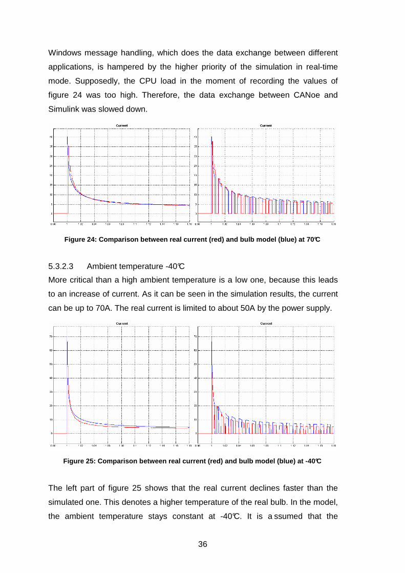
5.3.2.2 Ambient temperature 70°C

A higher ambient temperature reduces the current peak. Since this parameter

can be specified in the bulb model, it is possible to simulate this behavior. The

results are shown in figure 24. Both signals, real and simulated one, nearly

have the same amplitudes.

Conspicuously is the worse resolution of the real signal in contrast to the model.

The simulation has been executed with a sample time of 200µs. But the values

stay constant for about 1ms, which leads to bigger stairs in the plot. This

indicates that Simulink is supplied too slowly with new information. The real-

time simulation causes a higher CPU load. In order to get more system

ressources for the Simulink solver, the priorities in the Windows schedule

system are changed. This can be seen, for example, by a significantly higher

response time (e.g. for changing the active window). It is also possible that the

36

Windows message handling, which does the data exchange between different

applications, is hampered by the higher priority of the simulation in real-time

mode. Supposedly, the CPU load in the moment of recording the values of

figure 24 was too high. Therefore, the data exchange between CANoe and

Simulink was slowed down.

Figure 24: Comparison between real current (red) an d bulb model (blue) at 70°C

5.3.2.3 Ambient temperature -40°C

More critical than a high ambient temperature is a low one, because this leads

to an increase of current. As it can be seen in the simulation results, the current

can be up to 70A. The real current is limited to about 50A by the power supply.

Figure 25: Comparison between real current (red) an d bulb model (blue) at -40°C

The left part of figure 25 shows that the real current declines faster than the

simulated one. This denotes a higher temperature of the real bulb. In the model,

the ambient temperature stays constant at -40°C. It is a ssumed that the

37

ambience is not heated up by the emitted energy. In reality, the glowing bulb is

going to heat its immediate environment. For example, the glass of the bulb has

a temperature of at least 600°C in steady state. To si mulate this, the bulb model

would require a second transfer function, which describes how the glass is

heated by the emitted energy of the filament. Furthermore, the hot glass again

emits energy to the ambience. These details are not modeled in the simulation,

since the currently used model is accurate enough for testing purposes.

In reality, the hot glass reduces the temperature difference between filament

and ambience and therefore the transfer of heat. When the filament has

reached a higher temperature, the discrepancy between model and reality is

less significant and both currents are nearly the same.

Finally, it can be seen that the bulb model is useful as a first approximation to

the real behavior, even in different temperature ranges.

5.3.3 Measurement of delays

In order to measure the delay time, after which the output of the IOcab’s PWM

module is updated after a changing value in Simulink, the time between a

logical one at LIMP and the activation of emergency light was examined.

Furthermore, the behavior of the SCLS model in fail mode can be tested, too.

Therefore, the IGN input is permanently set to logical one, by connecting the

supply voltage to a digital input of the IOcab. To start the test and activate

emergency light, the LIMP input is connected to supply voltage, too.

Normally, 10ms after a positive edge at LIMP, the SCLS should switch on

emergency light, as shown in figure 26, where the following signals are

recorded:

• The LIMP input of the SCLS model in Simulink (diagram on the upper left).

• The current calculated by the bulb model (diagram on the lower left).

• The voltage at the digital input of the IOcab (channel 2 of the oscilloscope).

• The current measured by the shunt (channel 1 of the oscilloscope).

38

Figure 26: Measurement of the delay time

As it can be seen on the oscilloscope plot on the right, the time to activate the

real bulb was 16.3ms. Normally, the complete time should be equal to the

debounce time (i.e. 10ms), as shown in the left diagram. The measured time

leads to a delay time of 6.3ms caused by reading in the input, transferring the

environment variables from CANoe to Simulink and back and updating the duty

cycle of the IOcab.

This delay time varies from 2ms up to 11.8ms. One reason for these high and

differing times may be the Windows message handling. Furthermore, it is

possible that the IOcab’s PWM module works similar to the one of the SCLS

and uses a timer, which determines the switch-on time. This would mean that it

can take one period of this timer until the new value is valid.

6 Considerations for future projects To conclude this paper, some steps, which could simplify or shorten similar

projects in the future, should be mentioned. For this purpose, the most time-

consuming stages are examined in detail. These are the development of the

SCLS model and the tests of all models.

Since a specification sheet of the SCLS existed at least a year before starting

the development of the HLD, it would have been possible to model the SCLS

much earlier. Perhaps, it would even be possible, to let such models develop by

student-trainees that got an introduction to Matlab/Simulink. Since the

debounce time debounce time delay time

complete time

complete time

39

development can start much earlier, it would not matter if it is slightly delayed

due to the lack of skills of the trainee.

Another problem concerns the different simulation modes in TargetLink. A

comparison between MIL and SIL simulation is only a verification of the fixed-

point arithmetic. It is not verified whether the model itself works according to the

specification. For these tests, it is necessary, to include additional blocks, which

have to be removed for the SIL tests. Therefore, both methods require different

files, which can lead to inconsistencies.

Testing is a big problem due to the huge complexity of the model’s interfaces

and the test vectors. Tools like CTE try to simplify the handling of this

complexity. Nevertheless, even in CTE it is hard not to loose the overview if the

model grows larger. Conventional tests specify signals that have to be changed

at distinct points of time. Model-based test cases require the value of every

signal at every time step. A tool, which could generate test vectors out of normal

test sequences, would be a great advantage. The tool has to consider special,

programmable rules, e.g. that the watchdog bit has to be toggled every 75ms,

even if the interval between two instructions in the test specification is longer.

Hence, it would be possible e.g. to switch a bulb on at a defined point of time

and switch it off after one minute, without specifying the time steps for toggling

the watchdog bit. This would lead to an enormous simplification in the creation

of test vectors.

Due to the growing importance of model-based development, it can be

expected that such tools will be developed in the future.

40

Bibliography

[1] H. Schlingloff, M. Conrad, H. Dörr, C. Sühl, “Modellbasierte

Steuergerätesoftwareentwicklung für den Automobilbereich”, GI-

Tagung "Automotive Safety and Security 2004 - Sicherheit und

Zuverlässigkeit für automobile Informationstechnik", Stuttgart,

October 2004

[2] UK Software House Ltd.,

http://www.uksh.com/about/software-development-life-cycle.php,

2 February 2006

[3] M. Kückens, S. Kersten, “Die Klassifikationsbaummethode zum

funktionalen Test technischer Systeme”, January 2004

[4] Hera GmbH & Co. KG,

http://www.hera-online.de/uk/fachliches/fachliches.php,

2 February 2006

[5] G. Brechmann et al., “Elektrotechnik Tabellen Energieelektronik”,

5. Auflage, Westermann Schulbuchverlag GmbH, 2004

Author biography

Stefan Ferstl works as software development engineer

at Continental Automotive Systems since 2006.

Ferstl was born in 1982 in Regensburg. After his final

secondary-school examinations at Donau-Gymnasium

Kelheim (final thesis: “Programming of a self-learning

computer game”), he studied Electrical Engineering

and Information Technology with area of concentration

in Automotive Electronics at Fachhochschule Ingol-

stadt. Within a scholarship program, he simultaneously

worked as student-trainee in the development of body

controllers at Continental. There, he wrote his bache-

lor’s thesis about “Model-based software development

of a high-level driver for a Smart Corner Light Switch

using Matlab/Simulink and TargetLink”, which served

as base of this paper.

Contact: stefan.ferstl@contiautomotive.com

Impressum Herausgeber Der Präsident der Fachhochschule Ingolstadt Esplanade 10 85049 Ingolstadt Telefon: 08 41 / 93 48 - 0 Fax: 08 41 / 93 48 - 200 E-Mail: info@fh-ingolstadt.de Druck Hausdruck Die Beiträge aus der FH-Reihe "Arbeitsberichte/ Working Papers" erscheinen in unregelmäßigen Abständen. Alle Rechte, insbesondere das Recht der Vervielfältigung und Verbreitung sowie der Übersetzung vorbehalten. Nachdruck, auch auszugsweise, ist gegen Quellenangabe gestattet, Belegexemplar erbeten. Internet Dieses Thema können Sie, ebenso wie die früheren Veröffentlichungen aus der FH-Reihe "Arbeitsberichte - Working Papers", unter der Adresse www.fh-ingolstadt.de nachlesen. ISSN 1612-6483