Approximations to Stochastic Dynamic Programsvia Information Relaxation Duality

Santiago R. Balseiro and David B. Brown

Fuqua School of BusinessDuke University

srb43@duke.edu, dbbrown@duke.edu

January 18, 2016

Abstract

In the analysis of complex stochastic dynamic programs (DPs), we often seek strong theoreticalguarantees on the suboptimality of heuristic policies: a common technique for obtaining such guaranteesis perfect information analysis. This approach provides bounds on the performance of an optimal policyby considering a decision maker who has access to the outcomes of all future uncertainties before makingdecisions, i.e., fully relaxed non-anticipativity constraints. A limitation of this approach is that in manyproblems perfect information conveys excessive power to the decision maker, which leads to weak bounds.In this paper we leverage the information relaxation duality approach of Brown, Smith, and Sun (2010) toshow that by including a penalty that punishes violations of these non-anticipativity constraints, we canderive stronger bounds and analytically characterize the suboptimality of heuristic policies in stochasticdynamic programs that are too difficult to solve. We study three challenging problems: stochasticscheduling on parallel machines, a stochastic knapsack problem, and a stochastic project completionproblem. For each problem, we use this approach to derive analytical bounds on the suboptimality gapof a simple policy. In each case, these bounds imply asymptotic optimality of the policy for a particularscaling that renders the problem increasingly difficult to solve. As we discuss, the penalty is crucial forobtaining good bounds, and must be chosen carefully in order to link the bounds to the performance ofthe policy in question. Finally, for the stochastic knapsack and stochastic project completion problems,we find in numerical examples that this approach performs strikingly well.

Subject classifications: Dynamic programming, information relaxation duality, asymptotic optimality,stochastic scheduling, stochastic knapsack problems, stochastic project completion.

1 Introduction

Dynamic programming (DP) is a powerful and widely used framework for studying sequential decision-

making in the face of uncertainty. Unfortunately, stochastic dynamic programs are often far too difficult to

solve, as the number of states that need to be considered typically grows exponentially with the problem

size. As a result, we are often relegated to consider suboptimal, heuristic policies. In specific problem

instances, a variety of methods, often employing Monte Carlo simulation, may be used to assess the quality

of heuristic policies. More broadly, we may also seek strong analytical guarantees on the performance of

heuristic policies. Ideally, this analysis will allow us to conclude that a heuristic policy provides a good

approximation to the optimal policy on all instances, or at least allow us to understand on what types of

instances the heuristic policy will perform well.

A common technique in the analysis of heuristic policies is “perfect information analysis.” This approach

provides bounds by considering a decision maker who has advance access to the outcomes of all future

uncertainties, i.e., a problem with fully relaxed non-anticipativity constraints. We refer to this as the perfect

information problem. For each sample path, the decision maker then solves a deterministic optimization

problem, which is often easier to analyze than the original, stochastic DP. The typical analysis compares

the expected performance of the heuristic policy under consideration with the expected performance of the

perfect information problem, or the perfect information bound. This approach has been used successfully

in the analysis of heuristic policies in a number of applications; we survey a few in Section 1.1. In many

problems, however, perfect information may convey excessive power to the decision maker and lead to weak

bounds as a result: this limits the applicability of this approach.

Can we improve the quality of these bounds while retaining their amenability to theoretical analysis? In

this paper we provide a positive answer to this - in the context of three challenging DPs - by leveraging the

approach of Brown, Smith and Sun (2010) (BSS hereafter). The framework in BSS involves “information

relaxations” in which some (i.e., imperfect information) or all (i.e., perfect information) of the uncertainties

are revealed in advance, as well as a penalty that punishes violations of the non-anticipativity constraints.

BSS show both weak duality and strong duality: weak duality ensures that any penalty that is dual feasible

- in that it does not impose a positive, expected penalty on any non-anticipative policy - leads to an upper

bound on the expected reward with any policy, including an optimal policy. Strong duality ensures the

existence of a dual feasible penalty (albeit one that may be hard to compute) such that the upper bound

equals the expected reward with an optimal policy. Thus by including a dual feasible penalty we may be

able to improve the perfect information bounds. When we include a penalty, we refer to the optimization

problem in which we relax the non-anticipativity constraints as the penalized perfect information problem,

1

and the associated bound as the penalized perfect information bound.

To our knowledge, the use of information relaxations with penalties heretofore has been exclusively as a

computational method for evaluating heuristic policies in applications. Our objective in this paper is differ-

ent: we wish to use the approach to derive theoretical guarantees on the performance of heuristic policies

in complex DPs. Although our results provide analytical bounds that hold for all problem instances, we are

especially interested in identifying asymptotic regimes for which the heuristic policies in consideration ap-

proach optimality. We illustrate the approach in a study of three specific problems: (i) stochastic scheduling

on parallel machines, (ii) a stochastic knapsack problem, and (iii) a stochastic project completion problem.

In order to obtain theoretical guarantees, we consider simple heuristic policies that are amenable to analysis

and show that these simple policies approach optimality in a particular asymptotic regime. We study:

(i) Stochastic scheduling on parallel machines. This is the problem of scheduling a set of jobs on identical

parallel machines when no preemptions are allowed. Job processing times are stochastic and inde-

pendently distributed, and the processing times of each job are known only after a job is completed.

The goal is to minimize the total expected weighted completion time. We study the performance of

a greedy policy that schedules jobs in a fixed order based on weights and expected processing times,

and show that this policy is asymptotically optimal as the number of jobs grows large relative to the

number of machines. Although the result we derive is already known from Mohring et al. (1999) (and

a similar result is in Weiss (1990)), we provide an alternate and novel proof using a penalized perfect

information bound that allows us to exploit well-known results from deterministic scheduling.

(ii) Stochastic knapsack. In this problem (due to Dean et al., 2008), there is a set of items available to

be inserted to a knapsack of finite capacity. Each item has a deterministic value and a stochastic size

that is independently distributed. The actual size of an item is unknown until insertion of that item is

attempted. The decision maker repeatedly selects items for insertion until the capacity overflows, and,

at that moment, the problem ends. The goal is to maximize the expected value of all items successfully

inserted into the knapsack. We study the performance of a greedy policy that orders items based on

their values and expected sizes, and show that this policy is asymptotically optimal when the number

items grows and capacity is commensurately scaled.

(iii) Stochastic project completion. We consider a model of a firm working on a project that, upon comple-

tion, generates reward for the firm. A motivating example is a firm developing a new product, with

the reward being the expected NPV from launching the product. The firm is concurrently working on

different alternatives, and finishing any of these alternatives completes the project. In each period, the

firm can choose to accelerate one of the alternatives, at a cost. The goal is to maximize the total ex-

pected discounted reward over an infinite horizon. We consider static policies that commit exclusively

to accelerating the same alternative in every period, and show that these policies are asymptotically

optimal as the number of initial steps to completion grows large.

2

As we demonstrate in all three problems, the penalty is essential for obtaining a good bound. In each

problem, we provide a simple example that is easy to solve in closed form, but the perfect information bound

performs quite poorly. For example, in the stochastic knapsack problem, the perfect information problem

involves revealing all item sizes prior to any item selection decisions. When the decision maker knows the

realizations of all sizes in advance, she can avoid inserting potentially large items, which can result in weak

bounds. In Section 3 we reproduce a convincing example from Dean et al. (2008) for which these bounds

can be arbitrarily weak. With the inclusion of the penalty we consider, however, we recover a tight bound.

In each problem, we choose penalties carefully in order that they be: (a) dual feasible, so that we obtain

a bound; (b) simple enough so that we can analyze the bound; and (c) somehow connected to the heuristic

policy so that we can relate the bound to the performance of the heuristic policy. In all three problems, the

penalties cancel out information “locally” for each possible action at any point in time. For example, in the

stochastic knapsack problem, if we select an item in the penalized perfect information problem, we deduct a

penalty that is proportional to the difference between the expected size of the item and the realized size of

the item. This tilts incentives in the perfect information problem towards selecting items with large realized

sizes, which, absent the penalty, would be better to avoid in the perfect information problem. Such a penalty

does not completely counteract the benefit of perfect information, but by properly tuning the constants of

proportionality on the penalty, we can characterize the gap between the penalized perfect information bound

and the greedy policy and show that the greedy policy approaches optimality as the number of items (and

capacity) is scaled.

Finally, although our original goal in this paper was to develop these techniques for the sake of theoretical

analysis, we were surprised to also discover that the use of these “simple” penalties often led to strikingly

good performance in numerical examples. Specifically, we compute the bounds on many randomly generated

examples for the stochastic knapsack problem and the stochastic project completion problem and find small

gaps, particularly in comparison to other state-of-the-art approaches.

The rest of the paper is organized as follows. Section 1.1 reviews some related papers. Section 2

demonstrates the use of the approach on the stochastic scheduling problem, Section 3 discusses the stochastic

knapsack problem, and Section 4 discusses the stochastic project completion problem. These sections are

self-contained: in each section we begin by describing the problem and the perfect information bound, and

we then discuss the penalized perfect information bound and present our performance analysis. We conclude

Sections 3 and 4 with some numerical experiments that demonstrate the bounds. Section 5 concludes with

some guidance on how to apply these ideas to other problems. All proofs are available in Appendix B.

3

1.1 Literature review

In this section we discuss the connection of our work to several streams of literature. First, our paper

naturally relates to the literature on information relaxations. BSS draw inspiration from a stream of papers on

“martingale duality methods” aimed at calculating upper bounds on the price of high-dimensional, American

options, tracing back to independent developments by Haugh and Kogan (2004) and Rogers (2002). Rogers

(2007) independently developed similar ideas as in BSS for perfect information relaxations of MDPs using

change of measure techniques. In Appendix A we provide a review of the key definitions and results of

information relaxation duality.

In terms of applications of information relaxations, there are many other applications to options pricing

problems (Andersen and Broadie, 2004; BSS; Desai et al., 2012); inventory management problems (BSS;

Brown and Smith, 2014); valuation of natural gas storage (Lai et al., 2010; Nadarajah et al., 2015); inte-

grated models of procurement, processing, and commodity trading (Devalkar et al., 2011); dynamic portfolio

optimization (Brown and Smith, 2011; Haugh et al., 2014); linear-quadratic control with constraints (Haugh

and Lim, 2012); network revenue management problems (Brown and Smith, 2014); and multiclass queueing

systems (Brown and Haugh, 2014). Of central concern in these papers is computational tractability: the goal

is to use an information relaxation and penalty that render the upper bounds sufficiently easy to compute.

A recurring theme in these papers is that relatively easy-to-compute policies are often nearly optimal, and

the bounds computed from information relaxations are essential in showing this. Again, this line of work

focuses on numerically computing bounds for specific problem instances, while our objective in this paper is

to derive analytical guarantees on the performance of heuristic policies for a large class of problem instances.

Perfect information bounds (without penalty) have been successfully used in theoretically analyzing

heuristic policies in several applications in operations research and computer science, and are often referred

to as “hindsight bounds” or “offline optimal bounds.” Talluri and van Ryzin (1998) show that static bid-price

policies are asymptotically optimal in network revenue management when capacities and the length of the

horizon are large; they provide various upper bounds on the performance of the optimal policy, including

perfect information bounds. Feldman et al. (2010) study the online stochastic packing problem in the setting

where the underlying probabilistic model is unknown and show that a training based primal-dual heuristic is

asymptotically optimal when the number of items and capacities are large; they use the perfect information

bound as a benchmark. Manshadi et al. (2012) study the same problem when the underlying probability

distributions are known by the decision maker and present an algorithm that achieves at least 0.702 of the

perfect information bound. Garg et al. (2008) study the stochastic Steiner tree problem where each demand

vertex is drawn independently from some distribution and show that greedy policy is nearly optimal relative

4

to the perfect information bound. Similarly, Grandoni et al. (2008) study stochastic variants of set cover

and facility locations problems, and show that suitably defined greedy policies perform well with respect to

the expected cost with perfect information. Finally, in computer science there is a large body of work on

competitive analysis, which revolves around studying the performance of online algorithms relative to the

performance of an optimal “offline” algorithm that knows the entire input in advance. In this line of work

there is no underlying probabilistic model for the inputs and instead performance is measured relative to

the offline optimum in the worst-case (see, e.g., Borodin and El-Yaniv (1998) for a comprehensive review).

Stochastic scheduling is a fundamental problem in operations research with a vast literature, which we

do not attempt to review here; see Pinedo (2012) for a comprehensive review. In a key paper, Weiss (1990)

originally established the optimality gap of the WSEPT (Weighted Shortest Expected Processing Time first)

policy for scheduling on parallel machines and proved that this policy is asymptotically optimal under mild

conditions. Mohring et al. (1999) study polyhedral relaxations of the performance space of stochastic parallel

machine scheduling, and provide new sharp bounds on the performance of the WSEPT policy. We provide

an alternative and novel proof of the result in Mohring et al. (1999) using penalized perfect information

bounds. We carefully choose the penalty in a way that allows us to use the work of Hall et al. (1997) on

valid inequalities for deterministic scheduling.

The version of the stochastic knapsack problem we study was introduced in the influential paper by

Dean et al. (2008), although variants of this problem have been studied earlier. For example, Papstavrou

et al. (1996) study a version in which items arrive stochastically and in “take-it-or-leave-it” fashion; Dean

et al. (2008) provide an overview of earlier work. Dean et al. (2008) study both nonadaptive policies and

adaptive policies for the problem, and show that the loss for restricting attention to nonadaptive policies

is at most a factor of four. In addition, they provide sophisticated linear programming bounds based on

polymatroid optimization. The nonadaptive policy they consider is a greedy policy that inserts item in

decreasing order of the ratio of value to expected size. When item sizes are small relative to capacity, Dean

et al. (2008) show that the greedy policy performs within a factor of two of the optimal policy. Derman et al.

(1978) show that the greedy policy is optimal in the case of exponentially distributed sizes. Blado et al.

(2015) develop approximate dynamic programming style bounds for this problem and in extensive numerical

experiments find that the greedy policy often performs well, especially for examples with many items. In

this paper we show that the greedy policy approaches optimality as the number of items grows and capacity

is commensurately scaled.

Finally, the stochastic project completion is a new problem we developed and is motivated by a basic

tension faced by firms considering multiple alternatives in product development: how should firms optimally

invest in these alternatives, balancing costs with the pressure to develop a viable product quickly? This basic

5

tradeoff can arise in R&D settings in a host of industries (e.g., pharmaceutical, manufacturing, high tech,

etc.). Other papers have studied similar models. Childs and Triantis (1999) study dynamic R&D investment

policies with a variety of alternatives that may be accelerated or abandoned. Ding and Eliashberg (2002)

study decision tree models for a “pipeline problem” faced, e.g., by pharmaceutical companies. Santiago and

Vakili (2005) study firm R&D investment in which a single project can be managed “actively” (accelerated

to more favorable states through costly investment) or “passively” (continued in a baseline fashion). The

model we study involves a firm managing a potentially large number of alternatives over an infinite horizon.

This problem bears some resemblance to a restless bandit problem (Whittle, 1988) in that the states of

each alternative may change in each period, but differs in that the problem ends upon completion of any

alternative. The resulting DP can be quite challenging, but by using penalized perfect information analysis

we show that a static policy approaches optimality when the number of steps to completion grows large.

2 Illustrative example: stochastic scheduling on parallel machines

In this section, we demonstrate the use of the approach on a stochastic scheduling problem. Although the

main result in this section is already known from Mohring et al. (1999), we provide an alternative and novel

proof that uses penalized perfect information bounds.

Consider the problem of scheduling a set of jobs on identical parallel machines with the objective of

minimizing the total weighted completion time when no preemptions are allowed. Job processing times

are stochastic and the processing times of each job are known only after a job is completed. Formally, let

N = 1, . . . , n denote a set of jobs to be scheduled on m identical parallel machines. The processing time of

job i ∈ N is independent of the machine and given by the random variable pi. Processing times are assumed

to be independently distributed (but not necessarily identical) with finite second moments. Let Ci be the

completion time of job i ∈ N , that is, the sum of the waiting time until service and the processing time

pi. Each job has a weight wi and the objective is to minimize the expected total weighted completion time

E[∑ni=1 wiCi]. Using “Graham’s notation,” the problem can be written as PM//E[

∑i wiCi] (see Pinedo,

2012).

We let Π denote the set of non-anticipative, adaptive policies. A policy π ∈ Π is a mapping 2N×2N×Rn →

N that determines the next job to be processed, denoted by π(W,P, s), given the set of waiting jobs W ⊆ N ,

the set of jobs P ∈ N currently in process, and the amount of work done s ∈ Rn on each job in process. In this

model time is continuous and decision epochs correspond to the time when a job is completed and a machine

becomes available. We let Wπt ⊆ N denote the subset of jobs waiting for service at time t and Pπt ⊆ N denote

the subset of jobs under process at time t under policy π. Denoting the time when all jobs are completed

6

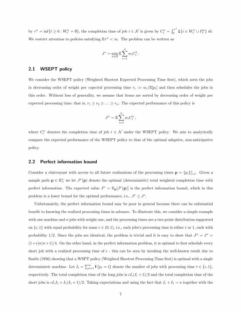
by τπ = inft ≥ 0 : Wπt = ∅, the completion time of job i ∈ N is given by Cπi =

∫ τπ0

1i ∈ Wπt ∪ Pπt dt.

We restrict attention to policies satisfying Eτπ <∞. The problem can be written as

J∗ = minπ∈Π

En∑i=1

wiCπi .

2.1 WSEPT policy

We consider the WSEPT policy (Weighted Shortest Expected Processing Time first), which sorts the jobs

in decreasing order of weight per expected processing time ri := wi/E[pi] and then schedules the jobs in

this order. Without loss of generality, we assume that items are sorted by decreasing order of weight per

expected processing time; that is, r1 ≥ r2 ≥ . . . ≥ rn. The expected performance of this policy is

JG = En∑i=1

wiCG

i ,

where CGi denotes the completion time of job i ∈ N under the WSEPT policy. We aim to analytically

compare the expected performance of the WSEPT policy to that of the optimal adaptive, non-anticipative

policy.

2.2 Perfect information bound

Consider a clairvoyant with access to all future realizations of the processing times p = pini=1. Given a

sample path p ∈ Rn+ we let JP(p) denote the optimal (deterministic) total weighted completion time with

perfect information. The expected value JP = Ep[JP(p)] is the perfect information bound, which in this

problem is a lower bound for the optimal performance, i.e., JP ≤ J∗.

Unfortunately, the perfect information bound may be poor in general because there can be substantial

benefit to knowing the realized processing times in advance. To illustrate this, we consider a simple example

with one machine and n jobs with weight one, and the processing times are a two-point distribution supported

on ε, 1 with equal probability for some ε ∈ (0, 1), i.e., each jobs’s processing time is either ε or 1, each with

probability 1/2. Since the jobs are identical, the problem is trivial and it is easy to show that JG = J∗ =

(1+ε)n(n+1)/4. On the other hand, in the perfect information problem, it is optimal to first schedule every

short job with a realized processing time of ε - this can be seen by invoking the well-known result due to

Smith (1956) showing that a WSPT policy (Weighted Shortest Processing Time first) is optimal with a single

deterministic machine. Let It =∑ni=1 1pi = t denote the number of jobs with processing time t ∈ ε, 1,

respectively. The total completion time of the long jobs is εIε(Iε + 1)/2 and the total completion time of the

short jobs is εIεI1 + I1(I1 + 1)/2. Taking expectations and using the fact that Iε + I1 = n together with the

7

fact that I1 is binomially distributed with n trials and success probability 1/2 since jobs are independent,

leads us to the poor lower bound of JP = n(n+ 3 + ε(3n+ 1))/8. Note that for n large, this lower bound is

off from J∗ by nearly a factor of two.

2.3 Penalized perfect information bound

Given a constant vector z = (zi)ni=1 ∈ Rn, we consider the integral Mπ

t =∫ t

0

∑i∈Wπ

szi(pi − E[pi]) ds. We

will use Mπτπ as a penalty. We claim Mπ

τπ is dual feasible in the sense of BSS, that is, Mπτπ does not penalize

in expectation any non-anticipative policy π ∈ Π:

E [Mπτπ ] = 0 . (1)

Condition (1) follows because, for every non-anticipative policy π ∈ Π, τπ is a stopping time and Mπτπ is a

martingale with respect to the natural filtration (i.e., the filtration that describes the decision maker’s state

of information at the beginning of the decision period). Hence the Optional Stopping Theorem implies that

E [Mπτπ ] = Mπ

0 = 0 because Eτπ <∞. We can express Mπτπ in terms of completion times as

Mπτπ =

n∑i=1

zi(pi − E[pi])Cπi − pizi(pi − E[pi]) ,

by adding and subtracting∫ τπ

0

∑i∈Pπs

zi(pi − E[pi]) ds and using the fact that pi =∫ τπ

01i ∈ Pπs ds.

Including the penalty, the scheduling problem becomes

J∗z = minπ∈Π

E

n∑i=1

(wi + zi(pi − E[pi]))Cπi

− E

n∑i=1

pizi(pi − E[pi]) ,

where we remove the terms that are independent of the scheduling policy from the minimization.

With perfect information and a given sample path p ∈ Rn+, let JPz (p) be the optimal total weighted

completion time including the penalty. We claim that JPz = Ep[JP

z (p)] is a lower bound on J∗. To see this,

for any π ∈ Π, we denote by Jπ and Jπz the expected weighted completion time of π with and without the

penalty, respectively; we then have

Jπ = Jπz ≥ JP

z ,

where the equality follows from (1) since the penalty is zero mean for any π ∈ Π and the inequality follows

from the fact that π is feasible for the problem with perfect information. This inequality holds for all π ∈ Π,

8

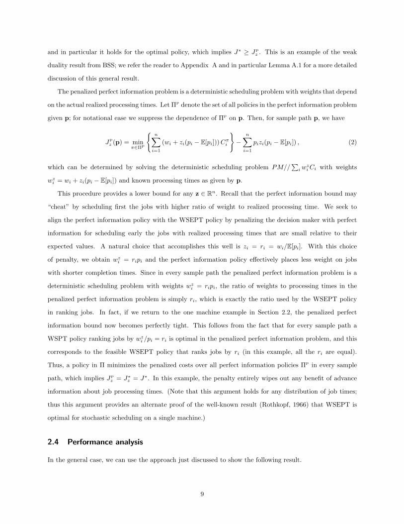
and in particular it holds for the optimal policy, which implies J∗ ≥ JPz . This is an example of the weak

duality result from BSS; we refer the reader to Appendix A and in particular Lemma A.1 for a more detailed

discussion of this general result.

The penalized perfect information problem is a deterministic scheduling problem with weights that depend

on the actual realized processing times. Let ΠP denote the set of all policies in the perfect information problem

given p; for notational ease we suppress the dependence of ΠP on p. Then, for sample path p, we have

JP

z (p) = minπ∈ΠP

n∑i=1

(wi + zi(pi − E[pi]))Cπi

−

n∑i=1

pizi(pi − E[pi]) , (2)

which can be determined by solving the deterministic scheduling problem PM//∑i w

ziCi with weights

wzi = wi + zi(pi − E[pi]) and known processing times as given by p.

This procedure provides a lower bound for any z ∈ Rn. Recall that the perfect information bound may

“cheat” by scheduling first the jobs with higher ratio of weight to realized processing time. We seek to

align the perfect information policy with the WSEPT policy by penalizing the decision maker with perfect

information for scheduling early the jobs with realized processing times that are small relative to their

expected values. A natural choice that accomplishes this well is zi = ri = wi/E[pi]. With this choice

of penalty, we obtain wzi = ripi and the perfect information policy effectively places less weight on jobs

with shorter completion times. Since in every sample path the penalized perfect information problem is a

deterministic scheduling problem with weights wzi = ripi, the ratio of weights to processing times in the

penalized perfect information problem is simply ri, which is exactly the ratio used by the WSEPT policy

in ranking jobs. In fact, if we return to the one machine example in Section 2.2, the penalized perfect

information bound now becomes perfectly tight. This follows from the fact that for every sample path a

WSPT policy ranking jobs by wzi /pi = ri is optimal in the penalized perfect information problem, and this

corresponds to the feasible WSEPT policy that ranks jobs by ri (in this example, all the ri are equal).

Thus, a policy in Π minimizes the penalized costs over all perfect information policies ΠP in every sample

path, which implies JPz = J∗z = J∗. In this example, the penalty entirely wipes out any benefit of advance

information about job processing times. (Note that this argument holds for any distribution of job times;

thus this argument provides an alternate proof of the well-known result (Rothkopf, 1966) that WSEPT is

optimal for stochastic scheduling on a single machine.)

2.4 Performance analysis

In the general case, we can use the approach just discussed to show the following result.

9

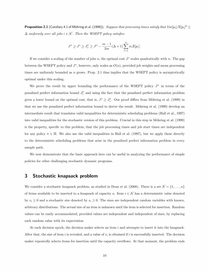
Proposition 2.1 (Corollary 4.1 of Mohring et al. (1999)). Suppose that processing times satisfy that Var[pi]/E[pi]2 ≤

∆ uniformly over all jobs i ∈ N . Then the WSEPT policy satisfies

JG ≥ J∗ ≥ JP

z ≥ JG − m− 1

2m(∆ + 1)

n∑i=1

wiE[pi] .

If we consider a scaling of the number of jobs n, the optimal cost J∗ scales quadratically with n. The gap

between the WSEPT policy and J∗, however, only scales as O(n), provided job weights and mean processing

times are uniformly bounded as n grows. Prop. 2.1 thus implies that the WSEPT policy is asymptotically

optimal under this scaling.

We prove the result by upper bounding the performance of the WSEPT policy JG in terms of the

penalized perfect information bound JPz and using the fact that the penalized perfect information problem

gives a lower bound on the optimal cost, that is, J∗ ≥ JPz . Our proof differs from Mohring et al. (1999) in

that we use the penalized perfect information bound to derive the result. Mohring et al. (1999) develop an

intermediate result that translates valid inequalities for deterministic scheduling problems (Hall et al., 1997)

into valid inequalities for the stochastic version of this problem. Crucial in this step in Mohring et al. (1999)

is the property, specific to this problem, that the job processing times and job start times are independent

for any policy π ∈ Π. We also use the valid inequalities in Hall et al. (1997), but we apply these directly

to the deterministic scheduling problems that arise in the penalized perfect information problem in every

sample path.

We now demonstrate that the basic approach here can be useful in analyzing the performance of simple

policies for other challenging stochastic dynamic programs.

3 Stochastic knapsack problem

We consider a stochastic knapsack problem, as studied in Dean et al. (2008). There is a set N = 1, . . . , n

of items available to be inserted to a knapsack of capacity κ. Item i ∈ N has a deterministic value denoted

by vi ≥ 0 and a stochastic size denoted by si ≥ 0. The sizes are independent random variables with known,

arbitrary distributions. The actual size of an item is unknown until the item is selected for insertion. Random

values can be easily accommodated, provided values are independent and independent of sizes, by replacing

each random value with its expectation.

At each decision epoch, the decision maker selects an item i and attempts to insert it into the knapsack.

After that, the size of item i is revealed, and a value of vi is obtained if i is successfully inserted. The decision

maker repeatedly selects items for insertion until the capacity overflows. At that moment, the problem ends

10

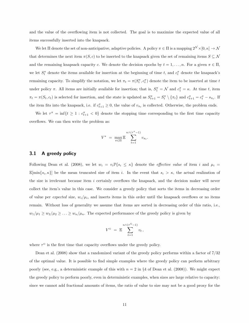
and the value of the overflowing item is not collected. The goal is to maximize the expected value of all

items successfully inserted into the knapsack.

We let Π denote the set of non-anticipative, adaptive policies. A policy π ∈ Π is a mapping 2N×[0, κ]→ N

that determines the next item π(S, c) to be inserted to the knapsack given the set of remaining items S ⊆ N

and the remaining knapsack capacity c. We denote the decision epochs by t = 1, . . . , n. For a given π ∈ Π,

we let Sπt denote the items available for insertion at the beginning of time t, and cπt denote the knapsack’s

remaining capacity. To simplify the notation, we let πt = π(Sπt , cπt ) denote the item to be inserted at time t

under policy π. All items are initially available for insertion; that is, Sπ1 = N and cπ1 = κ. At time t, item

πt = π(St, ct) is selected for insertion, and the state is updated as Sπt+1 = Sπt \ πt and cπt+1 = cπt − sπt . If

the item fits into the knapsack, i.e. if cπt+1 ≥ 0, the value of vπt is collected. Otherwise, the problem ends.

We let τπ = inft ≥ 1 : cπt+1 < 0 denote the stopping time corresponding to the first time capacity

overflows. We can then write the problem as:

V ∗ = maxπ∈Π

En∧(τπ−1)∑

t=1

vπt .

3.1 A greedy policy

Following Dean et al. (2008), we let wi = viPsi ≤ κ denote the effective value of item i and µi =

E[minsi, κ] be the mean truncated size of item i. In the event that si > κ, the actual realization of

the size is irrelevant because item i certainly overflows the knapsack, and the decision maker will never

collect the item’s value in this case. We consider a greedy policy that sorts the items in decreasing order

of value per expected size, wi/µi, and inserts items in this order until the knapsack overflows or no items

remain. Without loss of generality we assume that items are sorted in decreasing order of this ratio, i.e.,

w1/µ1 ≥ w2/µ2 ≥ . . . ≥ wn/µn. The expected performance of the greedy policy is given by

V G = En∧(τG−1)∑

t=1

vt ,

where τG is the first time that capacity overflows under the greedy policy.

Dean et al. (2008) show that a randomized variant of the greedy policy performs within a factor of 7/32

of the optimal value. It is possible to find simple examples where the greedy policy can perform arbitrary

poorly (see, e.g., a deterministic example of this with n = 2 in §4 of Dean et al. (2008)). We might expect

the greedy policy to perform poorly, even in deterministic examples, when sizes are large relative to capacity:

since we cannot add fractional amounts of items, the ratio of value to size may not be a good proxy for the

11

marginal value of adding an item.

There are, however, positive results for the greedy policy. Derman et al. (1978) show that the greedy

policy is optimal in the case of exponentially distributed sizes. Blado et al. (2015) conduct extensive numerical

experiments and find the greedy policy often performs well, especially for examples with many items. We

might expect the greedy policy to perform well when sizes are small relative to capacity: with many small

items, the problem “smoothes” in a certain sense. We can glean intuition for this from the deterministic case

by considering the LP relaxation of the problem that allows the decision maker to insert fractional items.

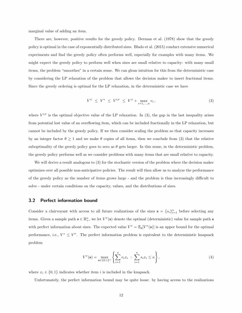
Since the greedy ordering is optimal for the LP relaxation, in the deterministic case we have

V G ≤ V ∗ ≤ V LP ≤ V G + maxi=1,...,n

vi , (3)

where V LP is the optimal objective value of the LP relaxation. In (3), the gap in the last inequality arises

from potential lost value of an overflowing item, which can be included fractionally in the LP relaxation, but

cannot be included by the greedy policy. If we then consider scaling the problem so that capacity increases

by an integer factor θ ≥ 1 and we make θ copies of all items, then we conclude from (3) that the relative

suboptimality of the greedy policy goes to zero as θ gets larger. In this sense, in the deterministic problem,

the greedy policy performs well as we consider problems with many items that are small relative to capacity.

We will derive a result analogous to (3) for the stochastic version of the problem where the decision maker

optimizes over all possible non-anticipative policies. The result will then allow us to analyze the performance

of the greedy policy as the number of items grows large - and the problem is thus increasingly difficult to

solve - under certain conditions on the capacity, values, and the distributions of sizes.

3.2 Perfect information bound

Consider a clairvoyant with access to all future realizations of the sizes s = sini=1 before selecting any

items. Given a sample path s ∈ Rn+, we let V P(s) denote the optimal (deterministic) value for sample path s

with perfect information about sizes. The expected value V P = Es[VP(s)] is an upper bound for the optimal

performance, i.e., V ∗ ≤ V P. The perfect information problem is equivalent to the deterministic knapsack

problem

V P(s) = maxx∈0,1n

n∑i=1

vixi :

n∑i=1

sixi ≤ κ

, (4)

where xi ∈ 0, 1 indicates whether item i is included in the knapsack.

Unfortunately, the perfect information bound may be quite loose: by having access to the realizations

12

of all sizes in advance, we can avoid inserting potentially large items. Dean et al. (2008) demonstrate this

convincingly with the following example: consider the case when all items are symmetric with value one,

and the sizes are a Bernoulli random variable with probability 1/2 scaled by κ+ ε for some ε > 0, i.e., each

item’s size is either 0 or κ+ ε with equal probability. Since the items are symmetric, the problem is trivial

and it is easy to show that V G = V ∗ = 1 − (1/2)n ≤ 1. On the other hand, in the perfect information

problem, it is optimal to select every item with a realized size of zero. Since this occurs with probability 1/2

for each item, and items are independent, this leads us to the very poor upper bound of V P = n/2.

3.3 Penalized perfect information bound

To improve the upper bound, we must impose a penalty that punishes violations of the non-anticipativity

constraints. Before proceeding, we first discuss a variation of the problem that will be helpful. Specifically,

the greedy policy ranks items using their effective values, so it will be useful for us to work with a variation

of the problem in which the values vi are replaced by the effective value wi. In this variation, we also need

to include the value of the overflowing item. This leads us to the formulation

W ∗ = maxπ∈Π

En∧τπ∑t=1

wπt ,

where the set of policies Π and the stopping time τπ are defined as before. We first show that this formulation

provides an upper bound.

Proposition 3.1. V ∗ ≤W ∗.

We now return to the penalty, which we apply to this effective value formulation. We use a vector of

weights z = (zi)ni=1 ∈ Rn and consider the partial sum Mπ

j =∑jt=1 zπt(sπt − µπt), where si = minsi, κ

and πt is the item to be inserted by the policy in consideration at time t. We use Mπτπ∧n as a penalty;

this is dual feasible in the sense of BSS in that it does not penalize, in expectation, any non-anticipative

policy. Dual feasibility follows because, for every non-anticipative policy π ∈ Π, τπ is a stopping time and

Mπt is a martingale with respect to the natural filtration. Thus the Optional Stopping Theorem implies that

E [Mπτπ∧n] = Mπ

0 = 0, since the stopping time τπ ∧ n is bounded.

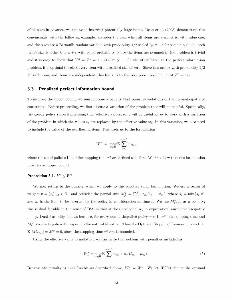
Using the effective value formulation, we can write the problem with penalties included as

W ∗z = maxπ∈Π

En∧τπ∑t=1

wπt + zπt(sπt − µπt) . (5)

Because the penalty is dual feasible as described above, W ∗z = W ∗. We let W Pz (s) denote the optimal

13

(deterministic) value of the penalized perfect information problem for sample path s ∈ Rn+. Since the set of

perfect information policies includes the set Π of non-anticipative policies, and the penalty is dual feasible, we

obtain an upper bound W ∗ ≤W Pz , where W P

z = Es[WPz (s)] denotes the penalized perfect information bound.

In Section C.1 we discuss how to calculate W Pz (s) by solving an integer program that includes additional

variables representing which item, if any, overflows the knapsack.

With this procedure, any z ∈ Rn provides an upper bound on W ∗, and hence by Proposition 3.1, on V ∗.

How should we choose z to get a good bound? Recall that the perfect information policy may “cheat” by

selecting items with relatively low realized sizes. The penalty we use seeks to align the perfect information

policy with the greedy policy by creating incentives for the decision maker with perfect information to resist

selecting items with realized sizes that are small relative to their expected sizes. In our analysis, we will use

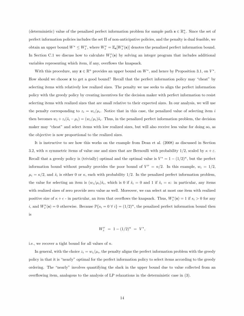
the penalty corresponding to zi = wi/µi. Notice that in this case, the penalized value of selecting item i

then becomes wi + zi(si−µi) = (wi/µi)si. Thus, in the penalized perfect information problem, the decision

maker may “cheat” and select items with low realized sizes, but will also receive less value for doing so, as

the objective is now proportional to the realized sizes.

It is instructive to see how this works on the example from Dean et al. (2008) as discussed in Section

3.2, with n symmetric items of value one and sizes that are Bernoulli with probability 1/2, scaled by κ+ ε.

Recall that a greedy policy is (trivially) optimal and the optimal value is V ∗ = 1 − (1/2)n, but the perfect

information bound without penalty provides the poor bound of V P = n/2. In this example, wi = 1/2,

µi = κ/2, and si is either 0 or κ, each with probability 1/2. In the penalized perfect information problem,

the value for selecting an item is (wi/µi)si, which is 0 if si = 0 and 1 if si = κ: in particular, any items

with realized sizes of zero provide zero value as well. Moreover, we can select at most one item with realized

positive size of κ+ ε - in particular, an item that overflows the knapsack. Thus, W Pz (s) = 1 if si > 0 for any

i, and W Pz (s) = 0 otherwise. Because Psi = 0 ∀ i = (1/2)n, the penalized perfect information bound then

is

W P

z = 1− (1/2)n = V ∗,

i.e., we recover a tight bound for all values of n.

In general, with the choice zi = wi/µi, the penalty aligns the perfect information problem with the greedy

policy in that it is “nearly” optimal for the perfect information policy to select items according to the greedy

ordering. The “nearly” involves quantifying the slack in the upper bound due to value collected from an

overflowing item, analogous to the analysis of LP relaxations in the deterministic case in (3).

14

3.4 Performance analysis

We now formalize the above discussion in the general case. We show that the greedy policy incurs a small

loss in value compared to the optimal policy when the scale of the problem increases, and in particular, that

the greedy policy is asymptotically optimal under conditions that we make precise.

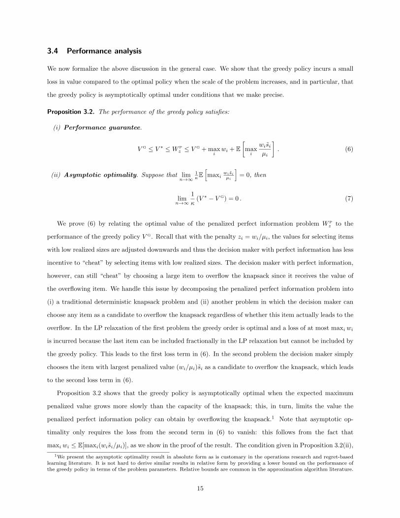
Proposition 3.2. The performance of the greedy policy satisfies:

(i) Performance guarantee.

V G ≤ V ∗ ≤W P

z ≤ V G + maxiwi + E

[maxi

wisiµi

]. (6)

(ii) Asymptotic optimality. Suppose that limn→∞

1κE[maxi

wisiµi

]= 0, then

limn→∞

1

κ(V ∗ − V G) = 0 . (7)

We prove (6) by relating the optimal value of the penalized perfect information problem W Pz to the

performance of the greedy policy V G. Recall that with the penalty zi = wi/µi, the values for selecting items

with low realized sizes are adjusted downwards and thus the decision maker with perfect information has less

incentive to “cheat” by selecting items with low realized sizes. The decision maker with perfect information,

however, can still “cheat” by choosing a large item to overflow the knapsack since it receives the value of

the overflowing item. We handle this issue by decomposing the penalized perfect information problem into

(i) a traditional deterministic knapsack problem and (ii) another problem in which the decision maker can

choose any item as a candidate to overflow the knapsack regardless of whether this item actually leads to the

overflow. In the LP relaxation of the first problem the greedy order is optimal and a loss of at most maxi wi

is incurred because the last item can be included fractionally in the LP relaxation but cannot be included by

the greedy policy. This leads to the first loss term in (6). In the second problem the decision maker simply

chooses the item with largest penalized value (wi/µi)si as a candidate to overflow the knapsack, which leads

to the second loss term in (6).

Proposition 3.2 shows that the greedy policy is asymptotically optimal when the expected maximum

penalized value grows more slowly than the capacity of the knapsack; this, in turn, limits the value the

penalized perfect information policy can obtain by overflowing the knapsack.1 Note that asymptotic op-

timality only requires the loss from the second term in (6) to vanish: this follows from the fact that

maxi wi ≤ E[maxi(wisi/µi)], as we show in the proof of the result. The condition given in Proposition 3.2(ii),

1We present the asymptotic optimality result in absolute form as is customary in the operations research and regret-basedlearning literature. It is not hard to derive similar results in relative form by providing a lower bound on the performance ofthe greedy policy in terms of the problem parameters. Relative bounds are common in the approximation algorithm literature.

15

while general, may be difficult to verify directly. The next result provides sufficient conditions that are easy

to check and are not very restrictive in order for asymptotic optimality to hold. We say an is little omega of

bn or an = ω(bn) if limn=∞ an/bn =∞, that is, an grows asymptotically faster than bn.

Corollary 3.3. Suppose that the ratios of value-to-size are uniformly bounded, that is, wi/µi ≤ r for some

r <∞ independent of the number of items n. Then (7) holds if:

(a) Sizes are uniformly bounded, that is, si ≤ s <∞, and capacity scales as κ = ω(1).

(b) Sizes have uniformly bounded means and variances, that is, E[si] ≤ m < ∞ and Var(si) ≤ σ2 < ∞,

and capacity scales as κ = ω(√n).

(c) Sizes are normally distributed with mean mi ≤ m < ∞ and standard deviation σi ≤ σ < ∞, and

capacity scales as ω(√

log n).

(d) Sizes are Pareto distributed with scale mi ≤ m < ∞ shape αi ≥ α > 0, and capacity scales as

κ = ω(n1/α).

Intuitively, the growth of the maximum penalized value maxi(wisi)/µi is governed to a large extent by the

tails of the distributions of sizes. When items are symmetric, roughly speaking, we have that E[maxi si] ≈

F−1(n/(n+ 1)) where F is the cumulative distribution function of sizes, and thus we need capacity to grow

at least as F−1(n/(n+ 1)) for (7) to hold. The previous result makes this intuition precise and provides the

necessary growth rate of capacity for different families of distributions. When sizes are uniformly bounded

(e.g., uniform or Bernoulli), the penalized values are trivially bounded and it suffices that capacity grow

unbounded at any rate. When sizes are normally distributed (an example of a light-tailed distribution), it

suffices that capacity grow at a logarithmic rate. Similar conditions can be verified as sufficient for sub-

gaussian distributions. When sizes are Pareto distributed (an example of a heavy-tailed distribution), it

suffices that capacity grow at a power-law rate.

3.5 Alternative bounds

In the performance analysis above, it was convenient to work with the effective value formulation, which

provides an upper bound on V ∗, as a starting point. This is helpful because it links to the greedy policy,

which uses effective values wi and mean truncated sizes µi. Although this suffices in our theoretical analysis,

in specific examples, the upper bound W ∗ itself may have some slack due to the fact that this formulation

receives full value for an item that overflows the knapsack.

We can also apply a penalty directly to the original formulation of the problem (i.e., with values and sizes

not adjusted, and no value received for an overflowing item). We use the same form of penalty as above,

16

except different values for the vector z. Including this penalty, the problem is

Vz = maxπ∈Π

E

n∧(τπ−1)∑t=1

vπt +

n∧τπ∑t=1

zπt(sπt − E[sπt ])

.As above, the penalty is mean zero for any feasible policy, so Vz = V ∗. The only differences between this

formulation and (5) are: (a) we use actual values and sizes rather than effective values and truncated sizes;

and (b) values can only be collected prior to overflow, as in the original statement of the problem. Note that

despite point (b), we must still include the penalty terms until τπ, i.e., until it is known that an overflow

has occurred. This is required to ensure dual feasibility of the penalty: for any feasible policy π ∈ Π, τπ is

a stopping time, but τπ − 1 is not.

With this approach, we now choose zi = vi/E[si], which is analogous to the choice above, except with

non-adjusted values and sizes. The optimal value with perfect information V Pz (s) for a given sample path

s can again be calculated as an integer program, very similar in form to that for W Pz (s) but with different

objective coefficients. This is discussed in Section C.2. We have found in our numerical examples that we

often get a stronger bound from V Pz = Es[V

Pz (s)] than W P

z ; although this need not always be true, this is

often the case due to the fact that V Pz (s) credits an overflowing item somewhat differently. (We can also use

the bound V Pz to derive a result similar to Prop. 3.2, but comparing to a greedy policy that ranks items by

vi/E[si]. Such a greedy policy, however, does not appear to be standard in the literature on this problem.)

In our examples, we also compare to upper bounds derived in Dean et al. (2008). Specifically, we also

calculate:

V DGV = max

n∑i=1

wixi :∑i∈S

µixi ≤ 2κ

(1−

∏i∈S

(1− µi)

)∀ S ⊆ N , 0 ≤ xi ≤ 1, ∀ i ∈ N

. (8)

Dean et al. (2008) show that V DGV ≥ V ∗ and that V DGV involves optimization over a polymatroid and can

thus be done easily following the greedy ordering; they also show that V DGV is a strengthening of an upper

bound from a deterministic LP relaxation that replaces sizes with their mean truncated sizes and allows the

knapsack to have double capacity (i.e., 2κ). The goals of the analysis in Dean et al. (2008) are somewhat

different than ours in that they seek constant factor approximation guarantees across all problem instances.

Dean et al. (2008) show that V DGV ≤ 4V ∗, a result that is useful in obtaining constant factor guarantees,

and also provide examples where this factor of 4 is nearly attained. Thus, we should not necessarily expect

V DGV to provide an especially good bound on a specific problem instance, but it does provide a benchmark

upper bound that is easy to compute.

Blado et al. (2015) provide sophisticated bounds based on approximate dynamic programming and find

17

that these bounds perform well in examples. These bounds, however, are somewhat involved to implement

(e.g., requiring column generation) and may be computationally challenging (e.g., Blado et al. (2015) report

runtimes of several hours on examples with n = 100). For these reasons, we did not attempt to calculate

these bounds.

3.6 Numerical examples

We demonstrate the upper bounds on a set of randomly generated examples. We consider n = 50, 100, 500,

and 1000. We generate values as vi ∼ U[0, 1] and mean sizes as E[si] ∼ U[0, 1], all i.i.d. Thus the mean value

of the expected sizes is 1/2, and we let κ = θn/2, where θ ∈ 1/8, 1/4, 1/2. The case θ = 1/8 corresponds

to tight capacity relative to the case θ = 1/2 (or, equivalently, relatively larger sizes in the θ = 1/8 case).

For each value of n and each value of θ, we randomly generate 20 sets of values and sizes as described above,

and for each set, we consider an instance with:

(i) Exponential sizes, with rate 1/E[si] for each item;

(ii) Bernoulli sizes, with probability 1/2, supported on 0, 2E[si] for each item; and

(iii) Uniform sizes, supported on [0, 2E[si]] for each item.

Note that, for consistency across the distributions, we are using the same values and mean sizes for each item

for a given instance. For each n, we have 20 instances for 3 different θ values and 3 different distributions,

or 180 total instances for each n.

For each instance, we calculate the lower bound V G corresponding to the greedy policy, and the upper

bounds corresponding to: (a) V Pz the perfect information bound with penalty as discussed in Section 3.5; (b)

W Pz the perfect information bound with penalty, using the effective value formulation; (c) V P, the perfect

information bound without penalty; and (d) the upper bound V DGV from Dean et al. (2008). All bounds

(other than V DGV, which does not require simulation) are estimated with 100 sample paths; this led to low

mean standard errors in the results. All calculations were done using Matlab on a desktop computer; we

used the MOSEK Optimization Toolbox for solving the integer programs in the upper bound calculations.

We note that for instances with n = 500 and n = 1000, we solved the LP relaxations for the integer programs

corresponding to W Pz and V P

z . This is of course sufficient to obtain upper bounds and had small impact on

the results while significantly reduces the runtime for these large instances. These bounds can be computed

efficiently in practice: for example, in instances with n = 1000 the calculation of V Pz , W P

z , and V P typically

took around 20 seconds per sample without much code optimization.

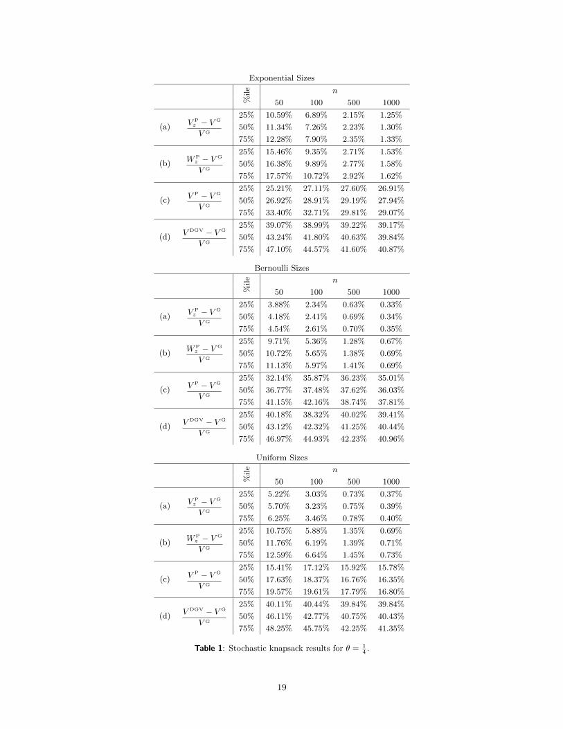
Table 1 summarizes the results for the intermediate value of θ = 1/4; the other results are similar and

in Section E of the appendix. Table 1 shows the 25th, 50th, and 75th percentiles of the gaps relative to the

18

Exponential Sizes

%ile n

50 100 500 1000

(a)V Pz − V G

V G

25% 10.59% 6.89% 2.15% 1.25%

50% 11.34% 7.26% 2.23% 1.30%

75% 12.28% 7.90% 2.35% 1.33%

(b)WP

z − V G

V G

25% 15.46% 9.35% 2.71% 1.53%

50% 16.38% 9.89% 2.77% 1.58%

75% 17.57% 10.72% 2.92% 1.62%

(c)V P − V G

V G

25% 25.21% 27.11% 27.60% 26.91%

50% 26.92% 28.91% 29.19% 27.94%

75% 33.40% 32.71% 29.81% 29.07%

(d)V DGV − V G

V G

25% 39.07% 38.99% 39.22% 39.17%

50% 43.24% 41.80% 40.63% 39.84%

75% 47.10% 44.57% 41.60% 40.87%

Bernoulli Sizes

%ile n

50 100 500 1000

(a)V Pz − V G

V G

25% 3.88% 2.34% 0.63% 0.33%

50% 4.18% 2.41% 0.69% 0.34%

75% 4.54% 2.61% 0.70% 0.35%

(b)WP

z − V G

V G

25% 9.71% 5.36% 1.28% 0.67%

50% 10.72% 5.65% 1.38% 0.69%

75% 11.13% 5.97% 1.41% 0.69%

(c)V P − V G

V G

25% 32.14% 35.87% 36.23% 35.01%

50% 36.77% 37.48% 37.62% 36.03%

75% 41.15% 42.16% 38.74% 37.81%

(d)V DGV − V G

V G

25% 40.18% 38.32% 40.02% 39.41%

50% 43.12% 42.32% 41.25% 40.44%

75% 46.97% 44.93% 42.23% 40.96%

Uniform Sizes

%ile n

50 100 500 1000

(a)V Pz − V G

V G

25% 5.22% 3.03% 0.73% 0.37%

50% 5.70% 3.23% 0.75% 0.39%

75% 6.25% 3.46% 0.78% 0.40%

(b)WP

z − V G

V G

25% 10.75% 5.88% 1.35% 0.69%

50% 11.76% 6.19% 1.39% 0.71%

75% 12.59% 6.64% 1.45% 0.73%

(c)V P − V G

V G

25% 15.41% 17.12% 15.92% 15.78%

50% 17.63% 18.37% 16.76% 16.35%

75% 19.57% 19.61% 17.79% 16.80%

(d)V DGV − V G

V G

25% 40.11% 40.44% 39.84% 39.84%

50% 46.11% 42.77% 40.75% 40.43%

75% 48.25% 45.75% 42.25% 41.35%

Table 1: Stochastic knapsack results for θ = 14.

19

greedy policy, across the 20 instances in each case. We report percentiles, rather than expected values, to

provide a better sense of the spread of the gaps. The bound V DGV (rows (d)) consistently leads to a gap of

around 40%. The perfect information bound without penalty V P (rows (c)) is also poor, although somewhat

better (e.g., gaps around 15 − 20% in the case of uniform sizes). These bounds alone shed no light on the

asymptotic optimality of the greedy policy for large n. The penalized perfect information bounds V Pz and

W Pz (rows (a) and (b), respectively) perform much better and clearly convey the asymptotic optimality of

the greedy policy. Typically, V Pz provides a stronger bound than W P

z , although the difference diminishes as

n grows. The gaps are somewhat larger with exponential sizes, as the distributions have heavier tails than

in the other cases; note that we know from existing results that greedy is optimal with exponential sizes, so

the gaps in examples with exponential sizes are solely due to the upper bounds. Tables 3 and 4 show similar

results, with somewhat larger (smaller) gaps with relatively tighter (looser) capacity, i.e., θ = 1/8 (θ = 1/2).

Although the theory tells us the penalized perfect information bounds must converge, we were surprised

by the performance of these bounds on these specific examples.

4 Stochastic project completion

We consider a model of a firm working on a project that, upon completion, generates reward for the firm.

A motivating example is a firm developing a new product, with the reward being the expected NPV from

launching the product. The firm is concurrently working on n different alternatives, and finishing any of these

alternatives completes the project. The firm faces uncertainty in completing these alternatives, and needs to

optimally balance development costs with the pressure to quickly complete the project. Although the model

we discuss is stylized, at a high level the model captures a problem faced by firms in a variety of industries,

where different alternatives are being considered towards some desired end goal, e.g. a pharmaceutical

company studying the efficacy of various compounds when developing a new cancer treatment, or a tech

company exploring the viability of different designs for a new smart phone.

Associated with each alternative i a state variable xi, which represents the number of steps remaining

to complete alternative i. In each period prior to the completion, the firm incurs a baseline cost of c0 ≥ 0,

which is the cost of concurrently working on all of the alternatives. Upon the first completion of any of the

n alternatives, i.e., when xi = 0 for any i, the firm generates a reward (i.e., an expected net present value of

future profits) of R = r/(1− δ), where r ≥ 0 and δ is the discount factor, and the problem ends.

Prior to completion, the state of each alternative evolves randomly and independently (over both time and

alternatives) according to a discrete-time Bernoulli process. Under baseline development, each alternative

transitions from xi to xi − 1 with probability qi or remains at xi with probability 1 − qi. If the state of

20

alternative i changes from xi to xi − 1, we say that alternative i improves. In each period, the firm can also

devote additional resources in an effort to accelerate the completion of an alternative. If the firm accelerates

alternative i in a given period, the cost of working in that period is ci ≥ c0, and alternative i improves with

probability pi ≥ qi; all other alternatives j 6= i improve with probability qj as in baseline development. We

assume the firm can accelerate at most one alternative per period. The goal is to maximize the expected

discounted reward over an infinite horizon.

This problem resembles a restless bandit problem in that the firm can either work “actively” (accelerate)

or “passively” (not accelerate) on alternatives in each period, and the states of alternatives evolve stochasti-

cally whether or not alternatives are accelerated. Distinguishing this problem from a restless bandit problem,

however, is a coupled termination condition: the problem ends upon completion of any alternative.

We can write this problem as a stochastic dynamic program with state variable x := (x1, . . . , xn). Prior

to completion, i.e., when xi > 0 for all i, the value function is

V (x) = maxi=0,...,n

−ci + δEV (x− di)

, (9)

and V (x) = R whenever xi = 0 for some i. In (9), the expectation is over di ∈ 0, 1n, which is a vector of

independent Bernoulli random variables such that dii = 1 with probability pi, and dij = 1 with probability

qj for all j 6= i. The random vector di captures the improvements across all alternatives when accelerating

alternative i. Note that because pi ≥ qi for all i, we can restrict to three outcomes for each alternative in

each period: (i) the alternative improves only if it is accelerated; (ii) the alternative improves regardless

of decision (i.e., under baseline development and if accelerated); and (iii) the alternative does not improve

regardless of decision. In (9), the index 0 represents the option of accelerating no alternative. Finally, we

let x0 denote the initial state, which we assume is known.

It will be convenient to write the expected reward of a given, feasible policy π, which maps from states

x to an action in 0, . . . , n. We denote this expected reward by V π and can write this as

V π = E

[δτ

π

R−τπ−1∑t=0

δtcπ(xt)

]= R− E

τπ−1∑t=0

δt(r + cπ(xt)

),

where τπ = inft : xπt,i = 0 for some i = 1, . . . , n denotes the stopping (completion) time of the policy, xπt

denotes the state process of the policy, and to simplify the notation we dropped the dependence on the initial

state x0. Thus, this problem is equivalent to a stochastic shortest path problem with discounting and costs

given by αi = r + ci when alternative i is accelerated. We let Π denote the set of feasible, non-anticipative

21

policies, and we can equivalently define the optimal reward as

V ∗ = R−minπ∈Π

Eτπ−1∑t=0

δtαπ(xt). (10)

From the principle of dynamic programming it follows that V ∗ = V (x0). Following (10), it will sometimes

be convenient to focus simply on the expected discounted costs until completion, and we will use J in place

of V accordingly, with the understanding that Jπ = R− V π.

We will assume that the acceleration costs are sufficiently small: specifically, we assume

ci − c0r + c0

≤ δ(pi − qi) , (11)

for i = 1, . . . , n. Although (11) does somewhat restrict our study of this problem, given that the firm views

the project as attractive to develop, we may expect acceleration costs would be small relative to rewards.

Note that (11) requires ci − c0 = 0 for any alternatives i such that pi = qi, which is intuitive: the marginal

cost of accelerating an alternative should be zero if accelerating the alternative provides no benefit. It can

also be shown that, in the simple case with n = 1 alternative in isolation and with one step to completion

remaining, (11) implies that acceleration is optimal.

4.1 Static policies

Solving for an optimal policy may be very difficult, as the number of states is exponential in n; if there

are many alternatives or several alternatives with many uncompleted steps, many possible states must be

considered in the recursion in (9). Intuitively, however, we may expect policies that accelerate alternatives

that appear most promising - as in, closest (or cheapest) to completion - to perform well. Motivated by this

intuition, we will study the quality of static policies, which commit to accelerating a fixed alternative (or

no alternative) in every state prior to completion. We can write the expected reward V Si of the ith static

policy, which accelerates alternative i in every period, as

V Si = R− αiEτSi−1∑t=0

δt = R− αi1− δ

· E[1− δτSi

]︸ ︷︷ ︸:=JSi

.

Analogous to above, τ Si denotes the stopping time of the ith static policy, which can be written as

τ Si = minY i1 , . . . , Y

in

, (12)

22

where Y ij is a negative binomial distribution supported on x0,j , x0,j + 1, . . . with x0,j successes and success

probability qj if j 6= i (or pj if j = i).2 Although calculating the exact distribution of τ i is difficult, we can

easily estimate V Si by evaluating (12) using Monte Carlo simulation. We then select the best static policy,

which has expected reward V S = maxi=0,...,n

V Si .

If the alternatives can never improve without acceleration, i.e., if qi = 0 for all i = 1, . . . , n, then a static

policy is optimal. This follows from the observation that in this case, if it is optimal to accelerate alternative

i in a given state, then it will also be optimal to accelerate i in the ensuing state: either the state of i

improves or it does not, and the states of all other alternatives do not change in this case. If qi > 0 for some

alternatives, however, a static policy will not be optimal in general: alternatives that are not accelerated in a

given period can nonetheless improve, and in later periods it may be optimal to accelerate such alternatives

if they become close enough to completion.

Although static policies are not generally optimal, we would expect the best static policy to perform well

in states close to completion. For example, when x0,i = 1 for all i, then it is straightforward to argue that

a static policy is optimal: in the next period, the firm will either complete some alternative or not. If not,

the state remains unchanged (x0,i = 1 for all i since no alternative was completed). Thus, there is only one

state to consider and a static policy is trivially optimal.

We will show that static policies perform well in the other extreme: namely, we will show that static

policies are asymptotically optimal in states far from completion. The asymptotic analysis that we consider

will focus on the case when the horizon effectively becomes very large, i.e., δ → 1, and the initial state

x0,i grows commensurately as O ((1− δ)−1). One interpretation of this scaling is that number of steps to

complete alternatives grows at the same rate as the length of the horizon (1− δ)−1, which is reminiscent of

the fluid scalings used in revenue management (see, e.g., Gallego and van Ryzin (1994)).

4.2 Perfect information bound

As a starting point for our analysis, we first consider the perfect information upper bound, which is given

by the expected reward of a firm that knows the future state transitions for all alternatives in advance. We

can write the optimal expected reward with perfect information V P as

V P = R− Ed minπ∈ΠP

τπ−1∑t=0

δtαπ, (13)

2We define a negative binomial distribution supported on x, x+1, . . . with x ∈ N successes and success probability p ∈ (0, 1](or NB(x, p) for short) as the total number of trials needed to get x successes when the probability of each individual successis p. The probability generating function is given by E

[zNB(x,p)

]= (zp/(1− (1− p)z))x for |z| ≤ 1/(1− p).

23

where the expectation is over the sample path d := (d0t , . . . ,d

nt )t≥0 describing alternative state transitions

in each period for each possible action (the sample path d is independent of the policy), and ΠP denotes the

set of all policies with perfect information on the particular sample path. It is clear that V P is an upper

bound on V ∗, since all non-anticipative, feasible policies are contained in ΠP.

In Appendix D.1 we show that the perfect information problem can be efficiently solved via Monte Carlo

simulation by using two observations. First, for every sample path d, the perfect information problem is

separable in the alternatives: that is, it suffices to find the policy that completes each alternative in isolation

with least cost and then take the associated alternative with the minimum cost. Second, we show that under

assumption (11) the optimal policy to complete alternative i in isolation has a simple structure: namely,

accelerate alternative i only in periods when the alternative requires acceleration to improve. (Note that if

(11) does not hold, the analysis is more complicated because always accelerating i in such periods need not

be optimal. For example, if the cost of acceleration is large, the perfect information policy may not accelerate

alternative i when this alternative can be improved shortly thereafter without acceleration. Thus, if (11)

does not hold, the optimal action in each period could depend on the remainder of the sample path.) Thus

the perfect information policy can “cheat” and save acceleration costs in time periods when an alternative

will improve without acceleration, as well as in time periods when the alternative will not improve even if

accelerated.

To illustrate the performance of the perfect information bound, we consider a simple example with n = 1

alternative, and the values r = 4, c0 = 0, c1 = 2δ, p1 = 1/2, and q1 = 0. These parameters satisfy assumption

(11) with equality. Since q1 = 0, the firm can never complete the alternative without accelerating it, and the

static policy that always accelerates this alternative is in fact optimal. The expected reward of this policy is

V S = R− α1

1− δ· E[1− δτ ] =

1

1− δ((4 + 2δ)Eδτ − 2δ) ,

where τ has a negative binomial distribution with parameters x1 and p1 = 1/2.

In the perfect information problem in this example, the firm observes d = (d0t , d

1t )t≥0 before making

acceleration decisions. Since q1 = 0, we have d0t = 0 in every period; that is, the alternative never improves

without acceleration. Also, with probability p1 = 1/2, d1t equals 1 in a given period, which corresponds to an

improvement of the alternative if the firm accelerates the alternative in period t. Conversely, with probability

1− p1 = 1/2, d1t = 0, which corresponds to no improvement of the alternative in period t, regardless of the

firm’s decision. It is clear that the optimal policy in the perfect information problem is, in all periods up

to completion, to accelerate the alternative (at cost r + c1) in periods when dt1 = 1 and to not accelerate

the alternative (at cost r) in periods when d1t = 0. Using this policy in (13), we can show that the optimal

24

expected reward with perfect information is

V P = R− (1− p1)r + p1(r + c1)

1− δ· E[1− δτ ] =

1

1− δ((4 + δ)Eδτ − δ) ,

where the first equality follows from a basic martingale argument (see Lemma B.3). The relative subopti-

mality gap then scales, when x1 = dx/(1− δ)e for some x > 0, as

(1− δ)(V P − V S) = δ (1− Eδτ ) −−−→δ→1

1− e−2x,

where the limiting expression follows from using the probability generating function for a negative binomial

random variable and taking limits. (The factor of 1 − δ normalizes the reward difference to be in units of

average reward per period and facilitates comparisons between different discount factors.)

This analysis on its own may lead one to conclude that, in the limit as the number of states grows to be

very large, static policies are suboptimal, perhaps significantly so, sacrificing an average per period reward

up to a constant factor of 1 − e−2x. This conclusion is false: as argued above, a static policy is optimal

for this problem. The gap in this analysis is arising from slack in the perfect information bound. In this

problem, there is substantial value to the information about the future state transitions of the alternatives,

and we require a penalty to compensate for this information and obtain a better upper bound.

4.3 Penalized perfect information bound

The perfect information problem does not provide a tight upper bound because, with advance knowledge

about state transitions, the firm can complete the project cheaply. In the example above, the firm can save

acceleration costs in time periods when d1t = 0, as the alternative will not improve in these periods even

with acceleration, whereas in the static (and optimal in that example) policy, the firm incurs acceleration

costs in every period prior to completion. We will attempt to improve the perfect information bound by

incorporating a penalty.

We will consider penalties that depend on the selected action in every period and d. The penalty in a

given time period t prior to completion when alternative i is accelerated is denoted zi(dt), where dt is the

period t component of d, i.e., dt = (d0t , . . . ,d

nt ) and the total discounted penalty is

∑τπ−1t=0 δtzπ(dt) when

the policy is π. Following BSS, in order to obtain an upper bound on V ∗, we require a dual feasible penalty:

Ed

[τπ−1∑t=0

δtzπ(dt)

]≤ 0 for all π ∈ Π. (14)

25

A sufficient condition for (14) is Edt [zi(dt)] ≤ 0 for each fixed action i since τπ − 1 is a stopping time. For

a given penalty z, we denote the optimal reward with perfect information by V Pz , which satisfies

V P

z = R− Ed minπ∈ΠP

τπ−1∑t=0

δt(απ + zπ(dt)).

Our goal is to find a penalty that (i) is dual feasible according to (14), and (ii) leads to an upper bound that

we can relate to the reward of the static policy. We first provide an intermediate result along these lines. In

the following, we denote by JPz = R− V P

z the penalized cost until completion with perfect information.

Proposition 4.1. There exists a dual feasible penalty z such that

JP

z =1

1− δEd min

i=1,...,n

τ i−1∑t=0

δt(αi + zi(dt)), (15)

where τ i is the completion time of alternative i when the firm accelerates i in every time period and, in

addition, Edt [αi + zi(dt)] ≥ (JS/JSi)αi for all i ∈ 1, . . . , n.

Proposition 4.1 states that we can find a dual feasible penalty and associated perfect information lower

bound (on costs) that is no smaller than the expected value of the best (penalized) static cost in every

sample path. This alone does not show that the static policy performs well, because the expectation in (15)

is outside the minimization; however, Proposition 4.1 also adds that the expected per stage penalized costs

are sufficiently large relative to the expected completion costs associated with the static policy. This latter

fact will be essential in using (15) to provide a bound on the performance of the static policy. The proof

of Proposition 4.1 describes explicitly a penalty that satisfies the desired properties. Before proceeding, we

provide some intuition for how this penalty works.

Recall that the perfect information policy can potentially “cheat” (incur no acceleration costs) in time

periods when alternatives will improve without acceleration (or not improve even with acceleration). The

penalty partially aligns the perfect information policy with the best static policy that aims to complete

alternative i by creating incentives for the decision maker with perfect information to accelerate i in every

period. The penalty accomplishes this by effectively reducing the acceleration costs for i in periods when

i will improve (or not) regardless of whether i is accelerated, but increasing the cost of accelerating i in

periods when i can only improve if accelerated. The proposed penalty carefully balances these cost changes

to ensure that the perfect information policy accelerates alternative i in all periods, and also to ensure that

the dual feasibility condition (14) holds, so that the procedure leads to an upper bound on V ∗.

26

4.4 Performance analysis

Proposition 4.1 leads us to our main result for this problem.

Proposition 4.2. Suppose (1 − δ)x0,i ≤ x for i = 1, . . . , n for some x independent of δ, and all other

parameters are held constant. Then the expected reward of the static policy satisfies:

(i) Performance guarantee. For some β independent of δ,

V S ≤ V ∗ ≤ V P

z ≤ V S +β√

1− δ.

(ii) Asymptotic optimality.

limδ→1

(1− δ) (V ∗ − V S) = 0.

Part (i) of Prop. 4.2 provides a uniform bound on the suboptimality of the static policy, and the proof of

this result in Appendix B.6 provides the constant β. Part (ii) of Prop. 4.2 is a straightforward consequence

of part (i) and states that the expected reward of the static policy approaches that of the optimal policy as

the number of states grow and δ approaches one. Note that part (i) characterizes the rate of convergence of

this asymptotic optimality.

What is the intuition for this result? We can imagine partitioning the state space into regions where

accelerating each alternative is the best action under the optimal policy. If it is ever optimal to accelerate

a particular alternative i, then it should be optimal to accelerate i when alternative i is much closer to

completion relative to all other alternatives. The static policy commits upfront to the alternative that, in

terms of costs, appears “closest” in the initial state. If this initial state is far from a boundary state where

the optimal policy would switch between accelerating alternatives, then, it is unlikely the alternative states

will ever evolve so as to reach this boundary. If the initial state is, on the other hand, close to one of these

boundary states, then it is relatively inconsequential which alternative is accelerated, as both are nearly

optimal. Either way, the difference in completion costs relative to the static policy will tend to be small as

the number of steps to completion grows.

4.5 Bounds from approximate dynamic programming

As a benchmark for the upper bounds described above, we also consider a bound based on the linear

programming approach to approximate dynamic programming (ADP). It is well-known that the optimal

value function can be calculated by formulating the DP (9) as a linear program with decision variables

corresponding to the value function in every possible state and constraints that impose Bellman optimality

27

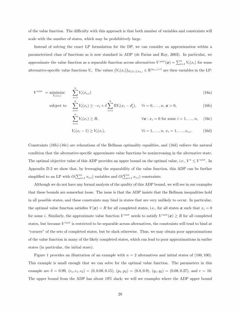
of the value function. The difficulty with this approach is that both number of variables and constraints will

scale with the number of states, which may be prohibitively large.

Instead of solving the exact LP formulation for the DP, we can consider an approximation within a

parameterized class of functions as is now standard in ADP (de Farias and Roy, 2003). In particular, we

approximate the value function as a separable function across alternatives V ADP(x) =∑ni=1 Vi(xi) for some

alternative-specific value functions Vi. The values Vi(xi)0≤xi≤x0,i∈ R|x0,i|+1 are then variables in the LP:

V ADP = minimizeVi(xi)

n∑i=1

Vi(x0,i) (16a)

subject to

n∑i=1

Vi(xi) ≥ −ci + δ

n∑i=1

EVi(xi − dij), ∀i = 0, . . . , n, x > 0, (16b)

n∑i=1

Vi(xi) ≥ R, ∀x : xi = 0 for some i = 1, . . . , n, (16c)

Vi(xi − 1) ≥ Vi(xi), ∀i = 1, . . . , n, xi = 1, . . . , x0,i. (16d)

Constraints (16b)-(16c) are relaxations of the Bellman optimality equalities, and (16d) enforce the natural

condition that the alternative-specific approximate value functions be nonincreasing in the alternative state.

The optimal objective value of this ADP provides an upper bound on the optimal value, i.e., V ∗ ≤ V ADP. In

Appendix D.2 we show that, by leveraging the separability of the value function, this ADP can be further

simplified to an LP with O(∑ni=1 x0,i) variables and O(

∑ni=1 x0,i) constraints.

Although we do not have any formal analysis of the quality of this ADP bound, we will see in our examples

that these bounds are somewhat loose. The issue is that the ADP insists that the Bellman inequalities hold

in all possible states, and these constraints may bind in states that are very unlikely to occur. In particular,

the optimal value function satisfies V (x) = R for all completed states, i.e., for all states x such that xi = 0

for some i. Similarly, the approximate value function V ADP needs to satisfy V ADP(x) ≥ R for all completed

states, but because V ADP is restricted to be separable across alternatives, the constraints will tend to bind at

“corners” of the sets of completed states, but be slack otherwise. Thus, we may obtain poor approximations

of the value function in many of the likely completed states, which can lead to poor approximations in earlier

states (in particular, the initial state).

Figure 1 provides an illustration of an example with n = 2 alternatives and initial states of (100, 100).

This example is small enough that we can solve for the optimal value function. The parameters in this

example are δ = 0.99, (c0, c1, c2) = (0, 0.08, 0.15), (p1, p2) = (0.8, 0.9), (q1, q2) = (0.08, 0.27), and r = 10.

The upper bound from the ADP has about 19% slack; we will see examples where the ADP upper bound

28

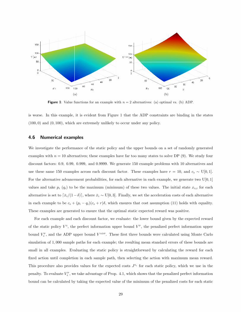
(a) (b)

Figure 1: Value functions for an example with n = 2 alternatives: (a) optimal vs. (b) ADP.

is worse. In this example, it is evident from Figure 1 that the ADP constraints are binding in the states

(100, 0) and (0, 100), which are extremely unlikely to occur under any policy.

4.6 Numerical examples

We investigate the performance of the static policy and the upper bounds on a set of randomly generated

examples with n = 10 alternatives; these examples have far too many states to solve DP (9). We study four

discount factors: 0.9, 0.99, 0.999, and 0.9999. We generate 150 example problems with 10 alternatives and

use these same 150 examples across each discount factor. These examples have r = 10, and c0 ∼ U[0, 1].

For the alternative advancement probabilities, for each alternative in each example, we generate two U[0, 1]

values and take pi (qi) to be the maximum (minimum) of these two values. The initial state x0,i for each

alternative is set to dxi/(1− δ)e, where xi ∼ U[0, 3]. Finally, we set the acceleration costs of each alternative

in each example to be c0 + (pi − qi)(c0 + r)δ, which ensures that cost assumption (11) holds with equality.

These examples are generated to ensure that the optimal static expected reward was positive.

For each example and each discount factor, we evaluate: the lower bound given by the expected reward

of the static policy V S, the perfect information upper bound V P, the penalized perfect information upper

bound V Pz , and the ADP upper bound V ADP. These first three bounds were calculated using Monte Carlo

simulation of 1, 000 sample paths for each example; the resulting mean standard errors of these bounds are

small in all examples. Evaluating the static policy is straightforward by calculating the reward for each

fixed action until completion in each sample path, then selecting the action with maximum mean reward.

This procedure also provides values for the expected costs JSi for each static policy, which we use in the

penalty. To evaluate V Pz , we take advantage of Prop. 4.1, which shows that the penalized perfect information

bound can be calculated by taking the expected value of the minimum of the penalized costs for each static

29

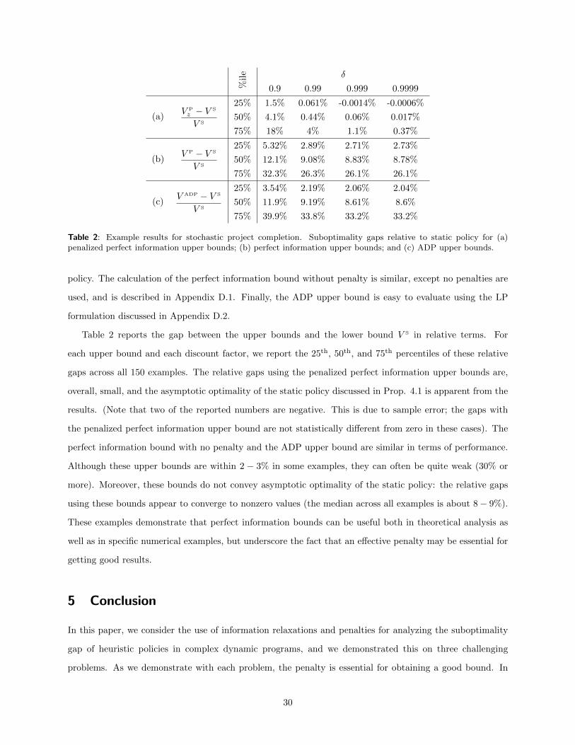
%il

e δ

0.9 0.99 0.999 0.9999

(a)V Pz − V S

V S

25% 1.5% 0.061% -0.0014% -0.0006%

50% 4.1% 0.44% 0.06% 0.017%

75% 18% 4% 1.1% 0.37%

(b)V P − V S

V S

25% 5.32% 2.89% 2.71% 2.73%

50% 12.1% 9.08% 8.83% 8.78%

75% 32.3% 26.3% 26.1% 26.1%

(c)V ADP − V S

V S

25% 3.54% 2.19% 2.06% 2.04%

50% 11.9% 9.19% 8.61% 8.6%

75% 39.9% 33.8% 33.2% 33.2%

Table 2: Example results for stochastic project completion. Suboptimality gaps relative to static policy for (a)penalized perfect information upper bounds; (b) perfect information upper bounds; and (c) ADP upper bounds.

policy. The calculation of the perfect information bound without penalty is similar, except no penalties are

used, and is described in Appendix D.1. Finally, the ADP upper bound is easy to evaluate using the LP

formulation discussed in Appendix D.2.

Table 2 reports the gap between the upper bounds and the lower bound V S in relative terms. For

each upper bound and each discount factor, we report the 25th, 50th, and 75th percentiles of these relative

gaps across all 150 examples. The relative gaps using the penalized perfect information upper bounds are,

overall, small, and the asymptotic optimality of the static policy discussed in Prop. 4.1 is apparent from the

results. (Note that two of the reported numbers are negative. This is due to sample error; the gaps with

the penalized perfect information upper bound are not statistically different from zero in these cases). The

perfect information bound with no penalty and the ADP upper bound are similar in terms of performance.

Although these upper bounds are within 2 − 3% in some examples, they can often be quite weak (30% or

more). Moreover, these bounds do not convey asymptotic optimality of the static policy: the relative gaps

using these bounds appear to converge to nonzero values (the median across all examples is about 8− 9%).

These examples demonstrate that perfect information bounds can be useful both in theoretical analysis as

well as in specific numerical examples, but underscore the fact that an effective penalty may be essential for

getting good results.

5 Conclusion

In this paper, we consider the use of information relaxations and penalties for analyzing the suboptimality

gap of heuristic policies in complex dynamic programs, and we demonstrated this on three challenging

problems. As we demonstrate with each problem, the penalty is essential for obtaining a good bound. In

30

each problem, we provide a simple example where the perfect information bound performs quite poorly, but

with the inclusion of a penalty we recover a tight bound.

We are hopeful that this technique can be applied successfully in many other problems, but the key is

finding a good penalty in the analysis. Although there is no general recipe to analyze the suboptimality of

heuristic policies in stochastic DPs, at a high level the steps involved in our approach are as follows. First, we

identify a heuristic policy and design a dual feasible penalty that somehow “aligns” the perfect information

policy with the heuristic policy in consideration. Second, we analyze the penalized perfect information

problem for each sample path using some problem specific technique. Finally, we take expectations of the

penalized perfect information problem over all sample paths and connect this upper bound (or lower bound

if costs) with the expected performance of the heuristic policy.

As was the case with the three problems we study here, what penalties will be effective depends on

the specifics of the problem. It may be helpful to summarize the intuition for why the penalties worked in

each of these three problems. First, in the stochastic scheduling problem we penalize the decision maker

with perfect information for scheduling early the jobs with realized processing times that are small relative

to their expected values. This tilts incentives in the perfect information problem towards scheduling early

jobs with long realized processing times, which, absent the penalty, would be scheduled later. We choose

the constants of proportionality on the penalty to make the ratio of weights to processing times in the

penalized perfect information problem exactly equal to the ratio used by the WSEPT policy in ranking

jobs. Second, in the stochastic knapsack problem, we deduct a penalty that is proportional to the difference

between the expected size of the item and the realized size of the item. Again this tilts incentives in the

perfect information problem towards selecting items with large realized sizes, which, absent the penalty,

would be better to avoid in the perfect information problem. We choose the constants of proportionality

on this penalty to make the ratio of value to size in the penalized perfect information bound exactly equal

to the ratio used by the greedy policy to select items. Third, in the stochastic project completion problem

the penalty increases the cost of acceleration in periods when an alternative can only be improved through

acceleration, and lowers costs otherwise. We choose these cost changes induced by the penalty to ensure that

it is optimal with perfect information to follow a policy that always accelerates one particular alternative in

every period until completion. Although the optimal such alternative varies across each sample path, this is

enough to align the perfect information policy with the best static policy that accelerates a fixed alternative.

Although penalized perfect information analysis weaves a common thread in our study of these problems,

we must acknowledge that problem specific battles in each problem remained in order to connect the penalized

perfect information bound with the expected performance of the heuristic policy. In the stochastic scheduling

problem, we use existing valid inequalities from deterministic scheduling and bound the penalized perfect

31

information problem via polymatroid optimization. In the stochastic knapsack problem, we cast the penalized

perfect information problem as a integer program and then apply LP relaxation bounds. In the stochastic

project completion problem, we decompose the penalized perfect information problem across the alternatives

and provide a bound on that decomposition. We believe that penalized perfect information analysis can be

effective in other problems, but we do not expect that problem-specific insights can be avoided.

Moving forward, it would be interesting to consider other problems with more complicated structure and

the need for more sophisticated policies and penalties. The policies we study here are all inherently non-

adaptive, and in many problems adaptivity may be essential for getting good performance. As for the penalty,

in each problem we study, the penalty punishes “local” violations of the non-anticipativity constraint, in

that at every point in time the penalty punishes the decision maker for actions viewed in isolation but does

not use the “global” system state. In other problems it might be necessary to consider more sophisticated

penalties that punish global violations of the non-anticipativity constraint, i.e., penalties that have explicit

state dependance.

32

A Review of Information Relaxation Duality

In this appendix we provide a review of information relaxation duality. The treatment here closely followsBSS. As in BSS, we consider the case where time is discrete and the horizon is finite; similar results can bederived for continuous time problems or infinite horizon problems.

A.1 The Primal Problem

Uncertainty in the DP is described by a probability space (Ω,F ,P) where Ω is the set of possible outcomesor scenarios ω, F is a σ-algebra that describes the set of possible events, and P is a probability measuredescribing the likelihood of each event.

Time is discrete and indexed by t = 0, . . . , T . The DM’s state of information evolves over time and isdescribed by a filtration F = (F0, . . . ,FT ) where the σ-algebra Ft describes the DM’s state of informationat the beginning of period t; we will refer to F as the natural filtration. The filtrations must satisfy Ft ⊆Ft+1 ⊆ F for all t < T so the DM does not forget what she once knew.

The DM must choose an action at in period t from a set At; we let A(ω) ⊆ A0 × · · · ×AT denote the setof all feasible action sequences a = (a0, . . . , aT ) given scenario ω. The DM’s choice of actions is describedby a policy π that selects a sequence of actions a in A for each scenario ω in Ω (i.e., π : Ω→ A). To ensurethe DM knows the feasible set when choosing actions in period t, we assume that the set of actions availablein period t depends on the prior actions (a0, . . . , at-1) and is Ft-measurable for each set of prior actions. Welet Π denote the set of all feasible policies, i.e., those that ensure that π(ω) is in A(ω).

In the primal problem, we require the DM’s choices to be nonanticipative in that the choice of action atin period t depends only on what is known at the beginning of period t; that is, we require policies to beadapted to the natural filtration F in that a policy’s selection of action at in period t must be measurablewith respect to Ft. We let ΠF be the set of feasible policies that are nonanticipative.

The DM’s goal is to select a feasible nonanticipative policy to maximize the expected total reward.The rewards are defined by a F-adapted sequence of reward functions (r0, . . . , rT ) where the reward rt inperiod t depends on the first t+1 actions (a0, . . . , at) of the action sequence a and the scenario ω. We let

r(a, ω) =∑Tt=0 rt(a, ω) denote the total reward. The primal DP is then:

supπ∈ΠF

E[ r(π) ] . (17)

Here E[ r(π) ] could be written more explicitly as E[ r(π(ω), ω) ] where policy π selects an action sequencethat depends on the random scenario ω and the rewards r depend on the action sequence selected by π andthe scenario ω. We suppress the dependence on ω and interpret r(π) as a random variable representing thetotal reward generated under policy π.

It will be helpful to rewrite the primal DP (17) as a Bellman-style recursion in terms of the optimal valuefunctions Vt. We let at = (a0, . . . , at) denote the sequence of actions up to and including period t. Sincethe period-t reward rt depends only on the first t+1 actions (a0, . . . , at), we will write rt(a) as rt(at) withthe understanding that the actions are selected from the full sequence of actions a; we will use a similarconvention for Vt. For t > 0, let At(at-1) be the subset of period-t actions At that are feasible given theprior choice of actions at-1: rt and At are both implicitly functions of the scenario ω. We take the terminalvalue function VT+1(aT ) = 0 and, for t = 0, . . . , T , we define

Vt(at-1) = supat∈At(at-1)

rt(at-1, at) + E[Vt+1(at-1, at) | Ft ]

. (18)

Here both sides are random variables (and therefore implicitly functions of the scenario ω) and we select anoptimal action at for each scenario ω.

A.2 Duality Results

In the dual problem, we relax the requirement that the policies be nonanticipative and impose penaltiesthat punish violations of these constraints. We define relaxations of the nonanticipativity constraints by

33

considering alternative information structures. We say that a filtration G = (G0, . . . ,GT ) is a relaxation ofthe natural filtration F = (F0, . . . ,FT ) if, for each t, Ft ⊆ Gt; we abbreviate this by writing F ⊆ G. G beinga relaxation of F means that the DM knows more in every period under G than she knows under F. Forexample, the perfect information relaxation is given by taking Gt = F for all t. We let ΠG denote the setof feasible policies that are adapted to G. For any relaxation G of F, we have ΠF ⊆ ΠG; thus, as we relaxthe filtration, we expand the set of feasible policies. In this paper, we will focus on the perfect informationrelaxation, where the set of relaxed policies is the set of all policies Π and actions are selected with fullknowledge of the scenario ω.

The set of penalties Z is the set of functions z that, like the total rewards, depend on actions a and thescenario ω. As with rewards, we will typically write the penalties as an action-dependent random variablez(a) (= π(a, ω)) or a policy-dependent random variable z(π) (= z(π(ω), ω)), suppressing the dependence onthe scenario ω. We define the set ZF of dual feasible penalties to be those that do not penalize nonanticipativepolicies in expectation, that is

ZF = z ∈ Z : E[ z(π) ] ≤ 0 for all π in ZF . (19)

Policies that do not satisfy the nonanticipativity constraints (and thus are not feasible to implement) mayhave positive expected penalties.

We can obtain an upper bound on the expected reward associated with any nonanticipative policy byrelaxing the nonanticipativity constraint on policies and imposing a dual feasible penalty, as stated in thefollowing weak duality lemma. BSS show that this result holds for any information relaxation G of F. Westate a simpler result for the perfect information relaxation.

Lemma A.1 (Weak Duality). If πF and z are primal and dual feasible respectively (i.e., πF ∈ ΠF and z ∈ ZF),then

E[ r(πF) ] ≤ supπ∈Π

E[ r(π)− z(π) ] = E

[sup

a∈A(ω)

r(a, ω)− π(a, ω)

]. (20)

Proof. With z and πF as defined in the lemma, we have

E[ r(πF) ] ≤ E[ r(πF)− z(πF) ] ≤ supπ∈Π

E[ r(π)− z(π) ] .

The first inequality holds because z ∈ ZF (thus E[ z(πF) ] ≤ 0) and the second because πF ∈ ΠF andΠF ⊆ Π.

Thus any dual feasible penalty will provide an upper bound on the expected reward generated by anyprimal feasible policy. If we minimize over the dual feasible penalties in (20), we obtain the dual of theprimal DP (17):

infz∈ZF

supπ∈Π

E[ r(π)− z(π) ]

. (21)

The following result shows that in principle, we could determine the maximal expected reward in the primalDP (17) by solving the dual problem (21). This result is analogous to the strong duality theorem of linearprogramming. We refer the reader to BSS for a proof of this result.

Theorem A.2 (Strong Duality). We have

supπ∈ΠF

E[ r(π) ] = infz∈ZF

supπ∈Π

E[ r(π)− z(π) ]

.

Furthermore, if the primal problem on the left is bounded, the dual problem on the right has an optimalsolution z? ∈ ZF that achieves this bound.

34

A.3 Penalties

BSS provides a general approach for constructing “good” penalties, based on a set of generating functions.We will show that we can, in principle, generate an optimal penalty using this approach.

Proposition A.3 (Constructing Good Penalties). Let (w0, . . . , wT ) be a sequence of generating functions definedon A × Ω where each wt depends only on the first t+1 actions (a0, . . . , at) of a. Define zt(a) = wt(a) −E[wt(a) | Ft ] and z(a) =

∑Tt=0 zt(a). Then, for all πF in ΠF, we have E[ zt(πF) | Ft ] = 0 for all t, and

E[ z(πF) ] = 0.

The result implies that the penalties z generated in this way will be dual feasible (i.e., E[ z(πF) ] ≤ 0 for πF

in ΠF), but is stronger in that it implies the inequality defining dual feasibility (19) holds with equality: i.e.,E[ z(π) ] = 0 for all π in ΠF. In this case, we say the penalty has no slack. A penalty that has slack cancertainly be improved by eliminating the slack. Good penalties are thus, by construction, dual feasible withno slack. We refer the reader to BSS for a proof and further discussion of this result.

Considering a sequence of generating functions (w0, . . . , wT ), we can write the dual problem recursivelyas follows. Take the terminal dual value function to be VT+1(aT ) = 0. For t = 0, . . . , T , we have

Vt(at-1) = supat∈At(at-1)

rt(at-1, at)− wt(at-1, at) + E[wt(at-1, at) | Ft ] + Vt+1(at-1, at)

. (22)

The expected initial value, E[V0

], provides an upper bound on the primal DP (17).

We can construct an optimal penalty using Proposition A.3 by taking the generating functions to be basedon the optimal DP value function given by (18). Specifically, if we take generating functions wt(a) = Vt+1(at),we obtain an optimal penalty of the form:

z?(a) =

T∑t=0

Vt+1(at)− E[Vt+1(at) | Ft ] . (23)

It is easy to show by induction that the dual value functions are equal to the corresponding primal valuefunctions, i.e., Vt = Vt. This is trivially true for the terminal values (both are zero). If we assume inductivelythat Vt+1 = Vt+1, terms cancel and (22) reduces to the expression for Vt given in equation (18). Thus, withthis choice of generating function, we obtain an optimal penalty that we refer to as the ideal penalty : theinner problem is equal to V0 in every scenario and, moreover, the primal and dual problems will have thesame sets of optimal policies.

Of course, in practice, we will not know the true value function and cannot construct this ideal penalty.The key to obtaining a good bound is to find a penalty that approximates the differences in the value functiongiven in (23).

B Proofs

B.1 Proof of Proposition 2.1

We prove the following chain of inequalities

JP

z ≤ J∗ ≤ JG ≤ JP

z +m− 1

2m(∆ + 1)

n∑i=1

wiE[pi] ,

where the penalty is given by zi = ri = wi/E[pi]. The first two inequalities in the chain follow trivially. Inthe remainder of the proof we prove the last inequality, that is, we aim to upper bound the performance ofthe WSEPT policy using the penalized perfect information policy. We prove the result in three steps. First,we upper bound the performance of the WSEPT policy. Second, we lower bound the objective value of thepenalized perfect information problem for a fixed realization of processing times. Finally, we combine theprevious bounds to bound the performance of the WSEPT policy in terms of the expected penalized perfectinformation bound.

35

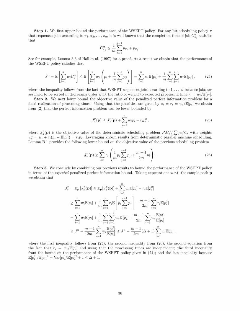
Step 1. We first upper bound the performance of the WSEPT policy. For any list scheduling policy πthat sequences jobs according to π1, π2, . . . , πn, it is well known that the completion time of job Cππj satisfiesthat

Cππj ≤1

m

j−1∑`=1

pπ` + pπj .

See for example, Lemma 3.3 of Hall et al. (1997) for a proof. As a result we obtain that the performance ofthe WSEPT policy satisfies that

JG = E

[n∑i=1

wiCG

i

]≤ E

n∑i=1

wi

pi +1

m

i−1∑j=1

pj

=

n∑i=1

wiE [pi] +1

m

n∑i=1

i−1∑j=1

wiE [pj ] , (24)

where the inequality follows from the fact that WSEPT sequences jobs according to 1, . . . , n because jobs areassumed to be sorted in decreasing order w.r.t the ratio of weight to expected processing time ri = wi/E[pi].

Step 2. We next lower bound the objective value of the penalized perfect information problem for afixed realization of processing times. Using that the penalties are given by zi = ri = wi/E[pi] we obtainfrom (2) that the perfect information problem can be lower bounded by

JP

z (p) ≥ JP

z (p) +

n∑i=1

wipi − rip2i , (25)

where JP

z (p) is the objective value of the deterministic scheduling problem PM//∑i w

ziCi with weights

wzi = wi + zi(pi − E[pi]) = ripi. Leveraging known results from deterministic parallel machine scheduling,Lemma B.1 provides the following lower bound on the objective value of the previous scheduling problem

JP

z (p) ≥n∑i=1

ri

1

mpi

i−1∑j=1

pj +m+ 1

2mp2i

. (26)

Step 3. We conclude by combining our previous results to bound the performance of the WSEPT policyin terms of the expected penalized perfect information bound. Taking expectations w.r.t. the sample path pwe obtain that

JP

z = Ep [JP

z (p)] ≥ Ep[JP

z (p)] +

n∑i=1

wiE[pi]− riE[p2i ]

≥n∑i=1

wiE[pi] +1

m

n∑i=1

riE

pi i−1∑j=1

pj

− m− 1

2m

n∑i=1

riE[p2i ]

=

n∑i=1

wiE[pi] +1

m

n∑i=1

i−1∑j=1

wiE [pj ]−m− 1

2m

n∑i=1

wiE[p2

i ]

E[pi]

≥ JG − m− 1

2m

n∑i=1

wiE[p2

i ]

E[pi]≥ JG − m− 1

2m(∆ + 1)

n∑i=1

wiE[pi] ,

where the first inequality follows from (25); the second inequality from (26); the second equation fromthe fact that ri = wi/E[pi] and using that the processing times are independent; the third inequalityfrom the bound on the performance of the WSEPT policy given in (24); and the last inequality becauseE[p2

i ]/E[pi]2 = Var[pi]/E[pi]

2 + 1 ≤ ∆ + 1.

36

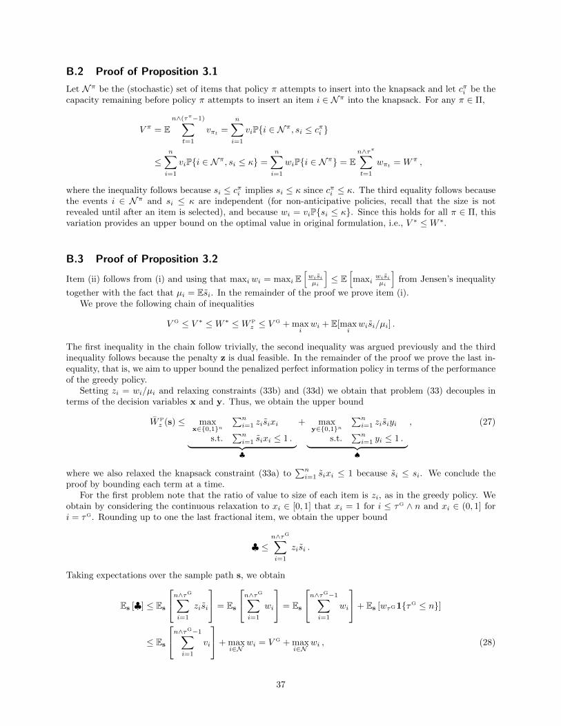
B.2 Proof of Proposition 3.1

Let N π be the (stochastic) set of items that policy π attempts to insert into the knapsack and let cπi be thecapacity remaining before policy π attempts to insert an item i ∈ N π into the knapsack. For any π ∈ Π,

V π = En∧(τπ−1)∑

t=1

vπt =

n∑i=1

viPi ∈ N π, si ≤ cπi

≤n∑i=1

viPi ∈ N π, si ≤ κ =

n∑i=1

wiPi ∈ N π = En∧τπ∑t=1

wπt = Wπ ,

where the inequality follows because si ≤ cπi implies si ≤ κ since cπi ≤ κ. The third equality follows becausethe events i ∈ N π and si ≤ κ are independent (for non-anticipative policies, recall that the size is notrevealed until after an item is selected), and because wi = viPsi ≤ κ. Since this holds for all π ∈ Π, thisvariation provides an upper bound on the optimal value in original formulation, i.e., V ∗ ≤W ∗.

B.3 Proof of Proposition 3.2

Item (ii) follows from (i) and using that maxi wi = maxi E[wisiµi

]≤ E

[maxi

wisiµi

]from Jensen’s inequality

together with the fact that µi = Esi. In the remainder of the proof we prove item (i).We prove the following chain of inequalities

V G ≤ V ∗ ≤W ∗ ≤W P

z ≤ V G + maxiwi + E[max

iwisi/µi] .

The first inequality in the chain follow trivially, the second inequality was argued previously and the thirdinequality follows because the penalty z is dual feasible. In the remainder of the proof we prove the last in-equality, that is, we aim to upper bound the penalized perfect information policy in terms of the performanceof the greedy policy.

Setting zi = wi/µi and relaxing constraints (33b) and (33d) we obtain that problem (33) decouples interms of the decision variables x and y. Thus, we obtain the upper bound

W P

z (s) ≤ maxx∈0,1n

∑ni=1 zisixi

s.t.∑ni=1 sixi ≤ 1 .︸ ︷︷ ︸♣

+ maxy∈0,1n

∑ni=1 zisiyi

s.t.∑ni=1 yi ≤ 1 .︸ ︷︷ ︸♠

, (27)

where we also relaxed the knapsack constraint (33a) to∑ni=1 sixi ≤ 1 because si ≤ si. We conclude the

proof by bounding each term at a time.For the first problem note that the ratio of value to size of each item is zi, as in the greedy policy. We

obtain by considering the continuous relaxation to xi ∈ [0, 1] that xi = 1 for i ≤ τG ∧ n and xi ∈ (0, 1] fori = τG. Rounding up to one the last fractional item, we obtain the upper bound

♣ ≤n∧τG∑i=1

zisi .

Taking expectations over the sample path s, we obtain

Es [♣] ≤ Es

n∧τG∑i=1

zisi

= Es

n∧τG∑i=1

wi

= Es

n∧τG−1∑i=1

wi

+ Es [wτG1τG ≤ n]

≤ Es

n∧τG−1∑i=1

vi

+ maxi∈N

wi = V G + maxi∈N

wi , (28)

37

where the first equality follows from considering the martingale Rt =∑ti=1 zisi−wi and using the Optional

Stopping Theorem to obtain that Es [Rn∧τG ] = 0; the second equality from excluding the overflowing item;the second inequality follows from the facts that wi = viPsi ≤ κ ≤ vi and wτG ≤ maxi∈N wi.

For the second problem note that the optimal solution selects the item with maximum objective and thus

♠ = maxi∈N

zisi . (29)

Taking expectations in equation (27) and using the bounds in (28) and (29) we obtain that

W P

z ≤ Es

[W P

z (s)]

= V G + maxi∈N

wi + E[maxi∈N

zisi] ,

as required because zi = wi/µi.

B.4 Proof of Corollary 3.3

Because the value-to-size ratios are bounded is suffices to show that En = 1κE [maxi=1,...,n minsi, κ] → 0

as n→∞. We prove each case at a time.

Case (a). This case follows trivially because En ≤ s/κ and κ = ω(1).

Case (b). Using minsi, κ ≤ si together with Theorem B.2 we obtain

En ≤1

κE[maxisi

]≤ 1

κmaxi

Esi +1

κ

√n− 1

n

∑i

Var(si) ≤m

κ+

√n

κσ ,

which converges to zero because κ = ω(√n).

Case (c). Some definitions are in order. We denote by x ≤sd y if random variable x is first-order stochasti-cally dominated by y, that is, Px ≤ z ≥ Py ≤ z for all z. Because si ∼ N (mi, σ

2i ) we have si ≤sd ti where

ti ∼ maxN (m, σ2), m. From extreme value theory we have that (maxi=1,...,n ti − an)/bn converges in dis-

tribution to a Gumbel random variable where an = m+ σ√

2 log(n)− σ log logn+log 4π2√

2 lognand bn = σ/

√2 log(n)

because the limit distribution is not sensitive to left truncation (Arnold et al., 2008, p.215). Lemma B.5implies that En → 0 as n→∞ when κ = ω

(max(an, bn)

)= ω

(√log(n)

).

Case (d). Because si is Pareto distributed with scale mi and shape αi we have si ≤sd ti where ti is Paretodistributed with scale m and shape α. From extreme value theory we have that (maxi=1,...,n ti − an)/bnconverges in distribution to a Frechet random variable where an = 0 and bn = n1/α (Arnold et al., 2008,p.215). Lemma B.5 implies that En → 0 as n→∞ when κ = ω

(max(an, bn)

)= ω

(n1/α

).

B.5 Proof of Proposition 4.1

We let ΠPi denote the set of perfect information policies that incur costs until (and do not garner rewards

until) alternative i is completed, and we use πi to denote a policy in ΠPi , with associated completion time

τ i. We first observe that, for any z such that αi + zi ≥ 0 for all i, and any sample path d,

minπ∈ΠP

τπ−1∑t=0

δt(απ + zπ(dt)) = mini=1,...,n

minπi∈ΠP

i

τ i−1∑t=0

δt(απi + zπi(dt)). (30)

To see this, let π? be a minimizer of the left-hand side; by the definition of τπ, the policy π? completes somealternative i?. Then π? ∈ ΠP

i? , and the costs on the right-hand side of (30) with πi? = π? will equal those onthe left-hand side. By minimizing over i, we can do no worse on the right-hand side. Conversely, let i? andπi? be a minimizer of the left-hand side. The policy πi? is feasible for the problem on the left-hand side andwill complete alternative i? in time τ i

?

, and perhaps some other alternative earlier. Since απ + zπ(·) ≥ 0 by

38

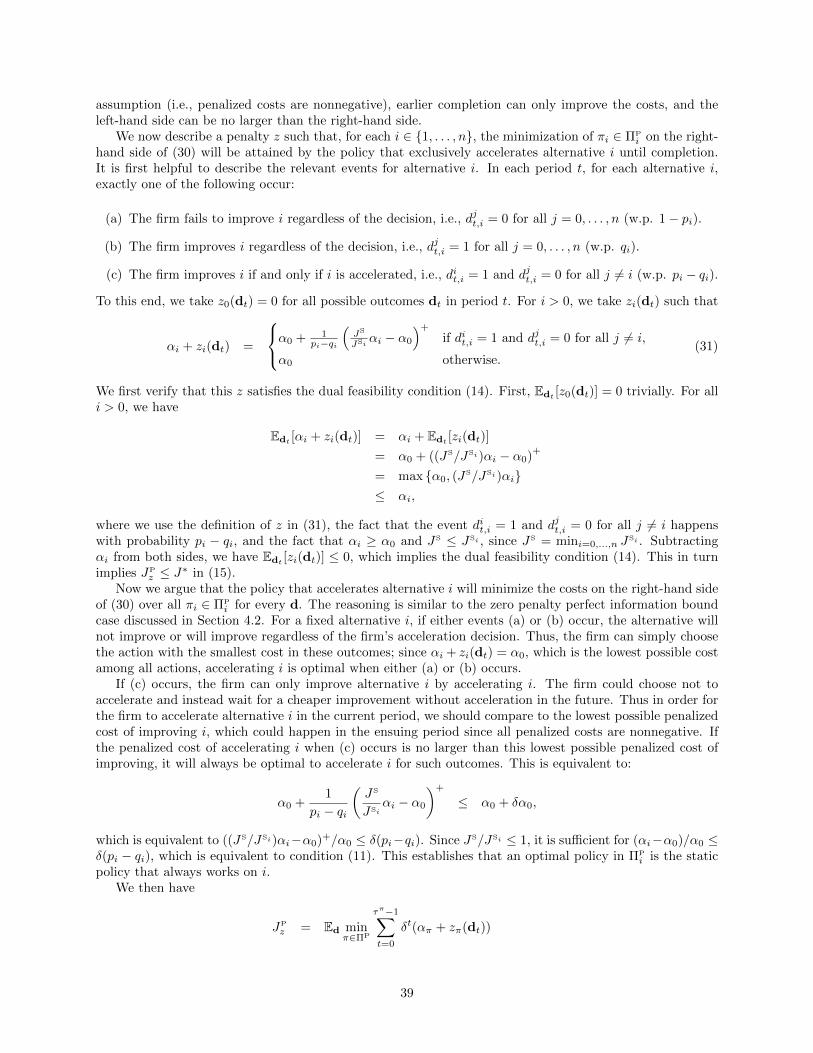
assumption (i.e., penalized costs are nonnegative), earlier completion can only improve the costs, and theleft-hand side can be no larger than the right-hand side.

We now describe a penalty z such that, for each i ∈ 1, . . . , n, the minimization of πi ∈ ΠPi on the right-

hand side of (30) will be attained by the policy that exclusively accelerates alternative i until completion.It is first helpful to describe the relevant events for alternative i. In each period t, for each alternative i,exactly one of the following occur:

(a) The firm fails to improve i regardless of the decision, i.e., djt,i = 0 for all j = 0, . . . , n (w.p. 1− pi).

(b) The firm improves i regardless of the decision, i.e., djt,i = 1 for all j = 0, . . . , n (w.p. qi).

(c) The firm improves i if and only if i is accelerated, i.e., dit,i = 1 and djt,i = 0 for all j 6= i (w.p. pi − qi).

To this end, we take z0(dt) = 0 for all possible outcomes dt in period t. For i > 0, we take zi(dt) such that

αi + zi(dt) =

α0 + 1pi−qi

(JS

JSiαi − α0

)+

if dit,i = 1 and djt,i = 0 for all j 6= i,

α0 otherwise.(31)

We first verify that this z satisfies the dual feasibility condition (14). First, Edt [z0(dt)] = 0 trivially. For alli > 0, we have

Edt [αi + zi(dt)] = αi + Edt [zi(dt)]

= α0 + ((JS/JSi)αi − α0)+

= max α0, (JS/JSi)αi

≤ αi,

where we use the definition of z in (31), the fact that the event dit,i = 1 and djt,i = 0 for all j 6= i happenswith probability pi − qi, and the fact that αi ≥ α0 and JS ≤ JSi , since JS = mini=0,...,n J

Si . Subtractingαi from both sides, we have Edt [zi(dt)] ≤ 0, which implies the dual feasibility condition (14). This in turnimplies JP

z ≤ J∗ in (15).Now we argue that the policy that accelerates alternative i will minimize the costs on the right-hand side

of (30) over all πi ∈ ΠPi for every d. The reasoning is similar to the zero penalty perfect information bound

case discussed in Section 4.2. For a fixed alternative i, if either events (a) or (b) occur, the alternative willnot improve or will improve regardless of the firm’s acceleration decision. Thus, the firm can simply choosethe action with the smallest cost in these outcomes; since αi + zi(dt) = α0, which is the lowest possible costamong all actions, accelerating i is optimal when either (a) or (b) occurs.

If (c) occurs, the firm can only improve alternative i by accelerating i. The firm could choose not toaccelerate and instead wait for a cheaper improvement without acceleration in the future. Thus in order forthe firm to accelerate alternative i in the current period, we should compare to the lowest possible penalizedcost of improving i, which could happen in the ensuing period since all penalized costs are nonnegative. Ifthe penalized cost of accelerating i when (c) occurs is no larger than this lowest possible penalized cost ofimproving, it will always be optimal to accelerate i for such outcomes. This is equivalent to:

α0 +1

pi − qi

(JS

JSiαi − α0

)+

≤ α0 + δα0,

which is equivalent to ((JS/JSi)αi−α0)+/α0 ≤ δ(pi−qi). Since JS/JSi ≤ 1, it is sufficient for (αi−α0)/α0 ≤δ(pi − qi), which is equivalent to condition (11). This establishes that an optimal policy in ΠP

i is the staticpolicy that always works on i.

We then have

JP

z = Ed minπ∈ΠP

τπ−1∑t=0

δt(απ + zπ(dt))

39

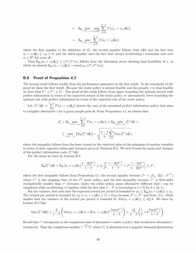
= Ed mini=1,...,n

minπi∈ΠP

i

τ i−1∑t=0

δt(απi + zπi(dt))

= Ed mini=1,...,n

τ i−1∑t=0

δt(αi + zi(dt))

where the first equality is the definition of JPz , the second equality follows from (30) and the fact that

αi + zi(dt) ≥ α0 ≥ 0, and the third equality uses the fact that always accelerating i minimizes cost overπi ∈ ΠP for every d.

That Edt [αi + zi(dt)] ≥ (JS/JSi)αi follows from the discussion above showing dual feasibility of z, inwhich we showed Edt [αi + zi(dt)] = maxα0, (J

S/JSi)αi.

B.6 Proof of Proposition 4.2

The second result follows readily from the performance guarantee in the first result. In the remainder of theproof we show the first result. Because the static policy is primal feasible and the penalty z is dual feasiblewe have that V S ≤ V ∗ ≤ V P

z . The proof of the result follows from upper bounding the optimal reward withperfect information in terms of the expected reward of the static policy, or alternatively lower bounding theoptimal cost with perfect information in terms of the expected cost of the static policy.

Let JP,iz (d) :=

τ i−1∑t=0

δt(αi + zi(dt)) denote the cost of the penalized perfect information policy that aims

to complete alternative i for a given sample path d. From Proposition 4.1 we obtain that

JP

z = Ed mini=1,...,n

τ i−1∑t=0

δt(αi + zi(dt)) = Ed mini=1,...,n

JP,iz (d) =

≥ mini=1,...,n

EdJ

P,iz (d)

−

√√√√n− 1

n

n∑i=1

Var(JP,iz (d)) ,

where the inequality follows from the lower bound on the expected value of the minimum of random variablesin terms of their expected values and variances given in Theorem B.2. We next bound the mean and varianceof the perfect information costs JP,i

z (d).For the mean we have by Lemma B.3

EdJP,iz (d) = Edt [αi + zi(dt)]

1− E[δτi

]

1− δ≥ αi

JS

JSi

1− E[δτi

]

1− δ= JS

1− E[δτi

]

1− E[δτSi ]≥ JS ,

where the first inequality follows from Proposition 4.1, the second equality because JSi = αi1−δ · E[1 − δτSi ]

where τ Si is the stopping time of the ith static policy, and the last inequality because τ Si is first-orderstochastically smaller than τ i (because, under the static policy, some alternative different that i can becompleted while accelerating i) together with the fact that 1− δt is increasing in t ∈ N for δ ∈ (0, 1).

For the variance, first note that the expected reward per period is bounded by α0 ≤ Edt [αi+zi(dt)] ≤ αi.The reward per period is bounded by α0 ≤ αi + zi(dt) ≤ (1 + δ)α0 because JS ≤ JSi and from (11), whichimplies that the variance of the reward per period is bounded by Var(αi + zi(dt)) ≤ α2

0/4. We have byLemma B.3 that

Var(JP,iz (d)) ≤ 2

1− δ

(Var(αi + zi(dt)) + E[αi + zi(dt)]

2 Var(δτi

)

1− δ

)≤ α2

0

1− δ

(1

2+ 8

Var(δτi

)

1− δ

).

Recall that τ i corresponds to the completion time of alternative i under a policy that accelerates alternative i

exclusively. Thus the completion satisfies τ i(d)= Y ii where Y ii is distributed as a negative binomial distribution

40

supported on x0,i, x0,j + 1, . . . with x0,j successes and success probability pi. Because (1 − δ)x0,i ≤ x,Lemma B.4 implies that

Var(δτi

) ≤ 2xai1− pipi

exp

(2x(ai − 1)

1− pipi

)︸ ︷︷ ︸

:=γi

(1− δ),

where ai = (4 + pi)/(2pi). Putting everything together, we obtain

JP

z ≥ JS − β√1− δ

,

where

β := α0

√√√√n− 1

n

n∑i=1

(1

2+ 8γi

),

and the first result follows.

B.7 Auxiliary results

The following result is a strengthened version of Lemma 3.2 from Hall et al. (1997) and provides a lowerbound on the objective value of the deterministic scheduling problem PM//

∑i ripiCi. We reproduce the

result for the sake of completeness.

Lemma B.1. The objective value of the deterministic scheduling problem PM//∑i ripiCi, denoted by JP

z (p),is lower bounded by

JP

z (p) ≥n∑i=1

ri

1

mpi

i−1∑j=1

pj +m+ 1

2mp2i

.

Proof. A lower bound on the objective value can be obtained from the observation that for any feasibleschedule on m machines the completion times should satisfy the following inequalities

∑i∈A

piCi ≥1

2m

(∑i∈A

pi

)2

+1

2

∑i∈A

p2i ,

for every subset A ∈ N (see, e.g., Hall et al. (1997)). Lemma 3.2 from Hall et al. (1997) proves a similarresult under a weaker class of valid inequalities.

Optimizing over the completion times we obtain that the latter deterministic scheduling problem can belower bounded by the following linear program

JP

z (p) ≥ minC∈Rn

n∑i=1

ripiCi

s.t.∑i∈A

piCi ≥ f(A) , ∀A ⊆ N , (32)

Ci ≥ 0 ,

where the set function f : 2N → R is given by f(A) = 12mp(A)2+ 1

2p2(A), where we denote by p(A) =

∑i∈A pi

and p2(A) =∑i∈A p

2i . It is not hard to see that the set function is super-modular, that is, for every j, k 6∈ A

we have that

f(A+ j) + f(A+ k) = f(A) + f(A+ j + k)− 2pjpk ≤ f(A) + f(A+ j + k) .

41

Setting yi = piCi we obtain that the feasible set of problem (32) is a polymatroid. Because the objectiveis linear in yi, we can apply the greedy algorithm of Edmonds to characterize its optimal solution. Sincethe objective’s coefficients satisfy r1 ≥ r2 ≥ . . . ≥ rn, we obtain that the optimal solution is given byy∗i = f(1, . . . , i)− f(1, . . . , i− 1), or equivalently that

y∗i = f(1, . . . , i)− f(1, . . . , i− 1)

=1

2m(p(1, . . . , i− 1) + pi)

2 − 1

2mp(1, . . . , i− 1)2 +

1

2p2i

=1

mpip(1, . . . , i− 1) +

m+ 1

2mp2i .

As a result the objective value is given by∑ni=1 riy

∗i , implying that

JP

z (p) ≥n∑i=1

riy∗i =

n∑i=1

ri

1

mpi

i−1∑j=1

pj +m+ 1

2mp2i

.

The following result provides an lower bound on the expected value of the minimum of random variables interms of their expected values and variances.

Theorem B.2 (Aven (1985)). For any sequence of random variables Xini=1 we have that E[miniXi] ≥mini EXi −

√n−1n

∑i Var(Xi) and E[maxiXi] ≤ mini EXi +

√n−1n

∑i Var(Xi).

We next provide bounds for moments of stopped discounted partial sums. Some definitions are in order. Let(yi)i≥1 ∈ N∞ be i.i.d. random variables and consider the partial sum Sn =

∑ni=1 yi. Let τ be the stopping

time corresponding to the first time that the partial sum hits a target X ∈ N, that is, τ = infn ≥ 1 : Sn =X. Let (zi)i≥1 ∈ N∞ be i.i.d. random variables with bounded support. We aim to bound the mean andvariance of the stopped discounted partial sum

C =

τ∑i=1

δi−1zi .

Here the process (zi)i≥1 need not be independent of the process (yi)i≥1.

Lemma B.3. Suppose that the stopping time τ is integrable and the increments zi have bounded support.

(i) Expected value. The expected value of the stopped discounted partial sum is given by:

E[C] = E[z1]1− E [δτ ]

1− δ.

(ii) Variance. The variance of the stopped discounted partial sum is bounded by:

Var (C) ≤ 2

1− δ

(Var(z1) + E[z1]2

Var(δτ )

1− δ

).

Proof. We first prove the result for the expected value and then prove the result for the variance.

Expected value. Consider the martingale Mn =∑ni=1 δ

i−1(zi −E[z1]) with M0 = 0. Because the stoppingtime τ is integrable and the increments zi have bounded support, we conclude by the Optional Stopping

42

Theorem that E[Mτ ] = 0. By construction we have that Mτ = C−E[z1]∑τi=1 δ

i−1. As a result the expectedvalue of the stopped partial sum is given by:

E[C] = E[z1]E

[τ∑i=1

δi−1

]= E[z1]

1− E [δτ ]

1− δ.

Variance. Consider the quadratic martingale Rn = M2n −Var(z1)

∑ni=1(δ2)i−1. Another application of the

Optional Stopping Theorem yields that E [Rτ ] = 0, which implies that E[M2τ

]= Var(z1)E

[∑τi=1(δ2)i−1

]=

Var(z1)(1− E[δ2τ])/(1− δ2) where Mτ = C − E[z1]

∑τi=1 δ

i−1. We can bound the variance as follows

√Var (C) = ‖C − E[C]‖2 ≤

∥∥∥∥∥C − E[z1]

τ∑i=1

δi−1

∥∥∥∥∥2

+

∥∥∥∥∥E[z1]

τ∑i=1

δi−1 − E[C]

∥∥∥∥∥2

= ‖Mτ‖2 +E[z1]

1− δ‖δτ − E [δτ ] ‖2

=

√Var(z1)

1− E [δ2τ ]

1− δ2+

E[z1]

1− δ√

Var(δτ )

where the first equation follows the definition of variance and denoting the L2 norm of X as ‖X‖2 =√

E[X2],and the first inequality follows from Minkowski’s inequality. From the AM-GM inequality we have that(√

a+√b)2

≤ 2(a+ b) for a, b > 0. Therefore

Var (C) ≤ 2Var(z1)1− E

[δ2τ]

1− δ2+ 2

E[z1]2

(1− δ)2Var(δτ )

≤ 2

1− δ

(Var(z1) + E[z1]2

Var(δτ )

1− δ

)where the second inequality follows from 1− δ2 ≥ 1− δ and 0 ≤ E

[δ2τ]

because τ ≥ 1 and δ ∈ (0, 1).

The next result bounds the variance of the random variable δτ , where τ captures the time to complete analternative when working exclusively on it.

Lemma B.4. Suppose τ is distributed as a negative binomial random variable supported on x, x + 1, . . .with x ∈ N successes and success probability p ∈ (0, 1). Then for δ ∈ (0, 1) we have:

Var(δτ ) ≤ zaez(a−1)(1− δ) ,

where z = 2x(1− δ) 1−pp and a = (4+p)

2p .

Proof. Using the probability generating function of the negative binomial random variable (see footnote 2)we obtain that the variance can be written as

Var(δτ ) = E[(δ2)τ]− E [δτ ]

2= δ2x

[(p

1− (1− p)δ2

)x︸ ︷︷ ︸

♣

−(

p

1− (1− p)δ

)2x

︸ ︷︷ ︸♠

].

The factor δ2x is trivially bounded as δ2x ≤ 1 because δ ∈ (0, 1) and x ≥ 0. In the remainder of the proofwe bound the terms in the parenthesis.

For the second term we have

♠ = exp

(2x log

(p

1− (1− p)δ

))≥ exp

(2x

(1− 1− (1− p)δ

p

))

43

= exp

(− 2x(1− δ)1− p

p

)= exp(−z) ,

where the first inequality follows because log x ≥ 1− 1x for x ≥ 0 and the last from setting z = 2x(1− δ) 1−p

p .For the first term we have

♣ = exp

(x log

(p

1− (1− p)δ2

))≤ exp

(x

(p

1− (1− p)δ2− 1

))= exp

(−x (1− p)(1− δ2)

1− (1− p)δ2

)= exp

(−z p(1 + δ)

2 (pδ2 + 1− δ2)

),

where the first inequality follows because log x ≤ x− 1 for x ≥ 0 and the last equality from the definition ofz and using that 1− δ2 = (1 + δ)(1− δ). The second factor in the exponential can be lower bounded as

p(1 + δ)

2 (pδ2 + 1− δ2)≥ p(1 + δ)

2 (p+ 2(1− δ))= 1− (4 + p)(1− δ)

2 (p+ 2(1− δ))≥ 1− (4 + p)

2p(1− δ) = 1− a(1− δ) ,

where the first inequality follows because δ ≤ 1 and (1− δ) = (1 + δ)(1− δ) ≤ 2(1− δ), the second inequality

from using that 1− δ ≥ 0 in the denominator, and the last equality from setting a = (4+p)2p .

Putting everything together, we obtain

Var(δτ ) ≤ ♣−♠ ≤ e−z(eza(1−δ) − 1

)≤ zaez(a−1)(1− δ) ,

where the inequality follows because ec(1−δ) − 1 ≤ cec(1− δ) for c ≥ 0 and δ ∈ (0, 1).

The following result bounds the growth of the expected value of the maximum of a sequence of randomvariables when the appropriately normalized maximum of this same sequence converges in distribution.

Lemma B.5. Let (si)∞i=1 be a sequence of non-negative i.i.d. random variables such that (maxi=1,...,n si −

an)/bn converges in distribution to some random variable Z where (an)∞n=1 and (bn)∞n=1 are deterministicsequences with bn ≥ 0. Let

En =1

κnE[

maxi=1,...,n

minsi, κn].

Suppose that the sequence (κn)∞n=1 satisfies κn = ω(

max(an, bn)), then

limn=∞

En = 0 .

Proof. Let Mn = maxi=1,...,n si be the maximum among the first n random variables. The expression in

consideration can be written as En = E[min

Mn

κn, 1]

, where we used the fact that maximum and minimum

are commutative. Note thatMn

κn=bnκn

Mn − anbn

+anκn

.

By assumption we have that bn/κn → 0 and an/κn → 0 as n→∞, while (Mn− an)/bn ⇒ Z as n→∞. By

Slutsky’s Theorem we conclude that Mn/κn ⇒ 0, which implies that Mn/κnp−→ 0 in probability because the

limit is constant. Because the function minx, 1 is continuous in x we obtain by the continuous mapping

theorem that minMn/κn, 1p−→ 0. Because 0 ≤ minMn/κn, 1 ≤ 1 the sequence is uniformly integrable

and we conclude that En → 0 as required.

44

C Computing bounds for stochastic knapsack

In this section we explain how to solve the penalized perfect information problem for the stochastic knapsackproblem.

C.1 Integer programming formulation for W Pz (s)

To calculate W Pz (s), because the item that overflows the knapsack now counts towards the objective, we

need to explicitly account for the overflowing item, whenever it exists. We obtain an upper bound on thepenalized perfect information problem for a fixed sample path s by solving the integer programming problem

W P

z (s) := maxx,y∈0,1n

n∑i=1

(wi + zi(si − µi))(xi + yi)

s.t.

n∑i=1

sixi ≤ κ , (33a)

xi + yi ≤ 1 , ∀i ∈ N , (33b)n∑i=1

yi ≤ 1 , (33c)

n∑i=1

si(xi + yi) ≥ κ(1− xi) , ∀i ∈ N . (33d)

where xi ∈ 0, 1 indicates whether the item is selected and fits the knapsack, and yi ∈ 0, 1 indicates ifthe item overflows the knapsack. Constraint (33b) imposes that an item either fits the knapsack or overflowsit. Constraint (33c) guarantees that there is at most one overflowing item. Constraint (33d) requiresthe overflowing item, if one exists, causes the selected capacity to exceed the capacity of knapsack. Thisconstraint is vacuous when all items fit the knapsack, i.e., if there is no overflow. Note that we can only besure that W P

z (s) ≤ W Pz (s), because the “overflowing” item yi can be chosen to exactly match the capacity of

the knapsack. In order for item yi to actually overflow the knapsack we need to make inequality (33d) strict.When the distribution of item sizes are absolutely continuous or lattice (i.e., there exists some h > 0 suchthat P

si ∈ 0, h, 2h, . . .

= 1 for all i ∈ N ), replacing constraint (33d) by

∑ni=1 si(xi+yi) ≥ (κ+ε)(1−xi)

for some ε > 0 in problem (33) gives that W Pz (s) = W P

z (s). The bound given by W Pz (s), however, suffices for

our analysis.

C.2 Integer programming formulation for V Pz (s)

The calculation of V Pz (s) is similar to that of W P

z (s). We can obtain an upper bound on V Pz (s) for a fixed

sample path s by solving the integer programming problem

V P

z (s) := maxx,y∈0,1n

n∑i=1

(vi + zi(si − E[si]))xi +

n∑i=1

zi(si − E[si])yi

s.t.

n∑i=1

sixi ≤ κ , (34a)

xi + yi ≤ 1 , ∀i ∈ N , (34b)n∑i=1

yi ≤ 1 , (34c)

n∑i=1

si(xi + yi) ≥ κ(1− xi) , ∀i ∈ N . (34d)

45

Formulation (34) is essentially identical to (33), with the difference that we use values instead of effectivevalues, sizes instead of truncated sizes, and we do not receive value for the overflowing item (though theoverflowing item does affect the objective through the penalty in the terms involving yi). Again, as withW Pz (s), if the distribution of sizes is continuous or lattice, we could exactly obtain V P

z (s) by replacing theconstraints (34d) with

∑ni=1 si(xi + yi) ≥ (κ+ ε)(1−xi) for some ε > 0, but we nonetheless obtain an upper

bound with the integer program (34).

D Computing bounds for stochastic project completion

In this section we explain how to efficiently solve the perfect information problem and the approximatedynamic programming bound for the stochastic project completion problem.

D.1 Perfect information problem

In the perfect information problem, the firm observes the sample path d = (d0t , . . . ,d

nt )t≥0 before making

acceleration decisions, where dit,j ∈ 0, 1 indicates whether or not the alternative j improves in period twhen the firm accelerates alternative i. We let ΠP

i denote the set of perfect information policies that incurcosts until (and do not garner rewards until) alternative i is completed, and we use πi to denote a policy inΠPi , with associated completion time τ i. Following the steps of the proof of Proposition 4.1 we first observe

that for every sample path d,

minπ∈ΠP

τπ−1∑t=0

δtαπ = mini=1,...,n

minπi∈ΠP

i

τ i−1∑t=0

δtαπi . (35)

This implies that the perfect information problem is separable in the alternatives; that is, it suffices to findthe best policy that aims to complete each alternative in isolation and then take the alternative with theminimum cost.

In order to solve each inner minimization problem in the right-hand side of (35) it is first helpful todescribe the relevant events for alternative i. In each period t, for each alternative i, exactly one of thefollowing occur:

(a) The firm fails to improve i regardless of the decision, i.e., djt,i = 0 for all j = 0, . . . , n (w.p. 1− pi).

(b) The firm improves i regardless of the decision, i.e., djt,i = 1 for all j = 0, . . . , n (w.p. qi).

(c) The firm improves i if and only if i is accelerated, i.e., dit,i = 1 and djt,i = 0 for all j 6= i (w.p. pi − qi).

Because policy πi is only concerned about the previous three outcomes we can consider the alternative samplepath (d0

t,i, d1t,i)t≥0 with three outcomes generated independently over time with the following distribution:

(d0t,i, d

1t,i) =

(0, 0) (fail regardless), w.p. 1− pi,(1, 1) (improve regardless), w.p. qi,

(0, 1) (improve only if accelerated), w.p. pi − qi.

For a given sample path (d0t,i, d

1t,i)t≥0, the objective is to minimize the discounted costs until completion of

alternative i. If the outcome in a given period is improve (not improve) regardless, the optimal action in theperfect information problem is to not accelerate, since the alternative will improve (not improve) whetheror not the alternative is accelerated in that period.

Thus, the only case to consider is what the optimal action should be when (d0t,i, d

1t,i) = (0, 1), i.e., the

alternative will improve in a given period if and only if accelerated. For such outcomes, we claim it is alwaysoptimal to accelerate the alternative. If the firm were to not accelerate the alternative for such outcomes, atbest the firm could improve the alternative in the ensuing period at discounted cost δα0 = δ(r + c), which

46

occurs when an “improve regardless” outcome of (1, 1) occurs at t+ 1. Thus, for it to be optimal to always

accelerate when (d0t,i, d

1t,i) = (0, 1), it is sufficient that

αi︸︷︷︸cost of advancing at t

≤ α0 + δα0︸ ︷︷ ︸lowest possible cost of advancing at t+ 1 but not t

or, equivalently, (ci − c)/(r + c) ≤ δ, which is implied by (11).Thus, the optimal perfect information policy for alternative i is to accelerate in each period t prior to

completion if and only if (d0t,i, d

1t,i) = (0, 1). Since the alternative is improved in each period with probability

qi + pi − qi = pi, the completion time τ i of the perfect information policy satisfies is distributed as negativebinomial random variable supported on x0, x0 + 1, . . . with x0 successes and success probability pi. Thusthe optimal cost of completing alternative i in isolation is

minπi∈ΠP

i

τ i−1∑t=0

δtαπi =

τ i−1∑t=0

δt(α0 + 1(d0t,i,d1t,i)=(0,1) · (αi − α0)

)and the optimal perfect information expected reward is given by

V P = R− Ed mini=1,...,n

τ i−1∑t=0

δt(α0 + 1(d0t,i,d1t,i)=(0,1) · (αi − α0)

).

The latter bound can be efficiently computed via Monte Carlo simulation.

D.2 Approximate dynamic programming

Here we present a linear programming formulation for the ADP given in Section 4.5 with O(∑ni=1 x0,i)

variables and O(∑ni=1 x0,i) constraints. Using the separability of the value function under the alternative-

specific approximation we obtain that for i 6= 0 the constraints (16b) can be written as

ci ≥ [δpi (Vi(xi − 1)− Vi(xi))− (1− δ)Vi(xi)] +∑j 6=i

[δqj (Vj(xj − 1)− Vj(xj))− (1− δ)Vj(xi)] .

This constraint can be handled by introducing auxiliary variables zi and yi, and imposing instead thatci ≥ zi +

∑j 6=i yi together with

zi ≥ δpi (Vi(xi − 1)− Vi(xi))− (1− δ)Vi(xi) ,yi ≥ δqi (Vi(xi − 1)− Vi(xi))− (1− δ)Vi(xi) ,

for all i = 1 . . . n and xi = 1 . . . x0,i. Similarly for i = 0 we can write this constraint as c0 ≥∑nj=1 yj . Because

the value functions are non-increasing in the state, we can write the boundary constraints (16c) involving Rfor each i as

Vi(0) +

n∑j 6=i

Vj(x0,j) ≥ R ,

since Vj(xj) ≥ Vj(x0,j). Putting everything together we obtain the following LP:

V ADP = minVi(xi),zi,yi

n∑i=1

Vi(x0,i)

s.t. zi ≥ δpi (Vi(xi − 1)− Vi(xi))− (1− δ)Vi(xi) , ∀i = 1 . . . n, xi = 1 . . . x0,i ,

yi ≥ δqi (Vi(xi − 1)− Vi(xi))− (1− δ)Vi(xi) , ∀i = 1 . . . n, xi = 1 . . . x0,i ,

ci ≥ zi +∑j 6=i

yj , ∀i = 1 . . . n ,

47

c0 ≥n∑j=1

yj ,

Vi(0) +

n∑j 6=i

Vj(x0,j) ≥ R , ∀i = 1 . . . n ,

Vi(xi − 1) ≥ Vi(xi) , ∀i = 1 . . . n, xi = 1 . . . x0,i .

E Additional numerical results for stochastic knapsack

In this section we present additional numerical results for the stochastic knapsack problem for the caseswhen the load factor is θ = 1/8 (tight capacity) and when the load factor is θ = 1/2 (moderate capacity).

48

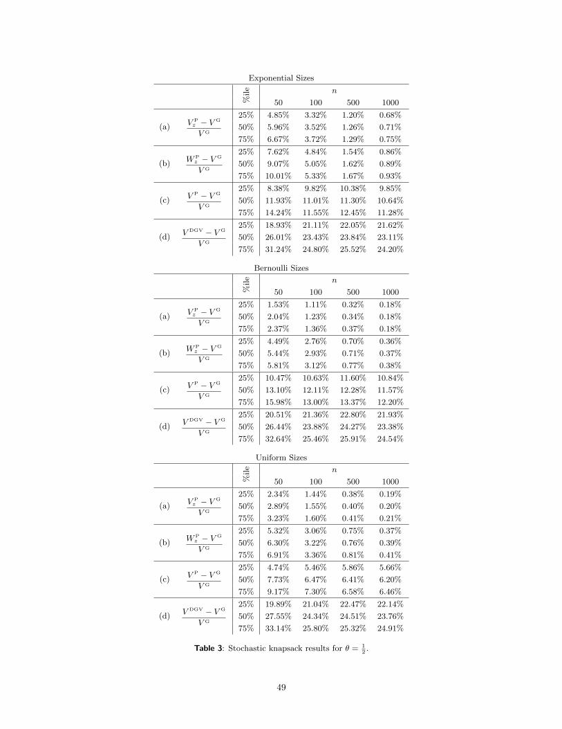
Exponential Sizes

%ile n

50 100 500 1000

(a)V Pz − V G

V G

25% 4.85% 3.32% 1.20% 0.68%

50% 5.96% 3.52% 1.26% 0.71%

75% 6.67% 3.72% 1.29% 0.75%

(b)WP

z − V G

V G

25% 7.62% 4.84% 1.54% 0.86%

50% 9.07% 5.05% 1.62% 0.89%

75% 10.01% 5.33% 1.67% 0.93%

(c)V P − V G

V G

25% 8.38% 9.82% 10.38% 9.85%

50% 11.93% 11.01% 11.30% 10.64%

75% 14.24% 11.55% 12.45% 11.28%

(d)V DGV − V G

V G

25% 18.93% 21.11% 22.05% 21.62%

50% 26.01% 23.43% 23.84% 23.11%

75% 31.24% 24.80% 25.52% 24.20%

Bernoulli Sizes

%ile n

50 100 500 1000

(a)V Pz − V G

V G

25% 1.53% 1.11% 0.32% 0.18%

50% 2.04% 1.23% 0.34% 0.18%

75% 2.37% 1.36% 0.37% 0.18%

(b)WP

z − V G

V G

25% 4.49% 2.76% 0.70% 0.36%

50% 5.44% 2.93% 0.71% 0.37%

75% 5.81% 3.12% 0.77% 0.38%

(c)V P − V G

V G

25% 10.47% 10.63% 11.60% 10.84%

50% 13.10% 12.11% 12.28% 11.57%

75% 15.98% 13.00% 13.37% 12.20%

(d)V DGV − V G

V G

25% 20.51% 21.36% 22.80% 21.93%

50% 26.44% 23.88% 24.27% 23.38%

75% 32.64% 25.46% 25.91% 24.54%

Uniform Sizes

%ile n

50 100 500 1000

(a)V Pz − V G

V G

25% 2.34% 1.44% 0.38% 0.19%

50% 2.89% 1.55% 0.40% 0.20%

75% 3.23% 1.60% 0.41% 0.21%

(b)WP

z − V G

V G

25% 5.32% 3.06% 0.75% 0.37%

50% 6.30% 3.22% 0.76% 0.39%

75% 6.91% 3.36% 0.81% 0.41%

(c)V P − V G

V G

25% 4.74% 5.46% 5.86% 5.66%

50% 7.73% 6.47% 6.41% 6.20%

75% 9.17% 7.30% 6.58% 6.46%

(d)V DGV − V G

V G

25% 19.89% 21.04% 22.47% 22.14%

50% 27.55% 24.34% 24.51% 23.76%

75% 33.14% 25.80% 25.32% 24.91%

Table 3: Stochastic knapsack results for θ = 12.

49

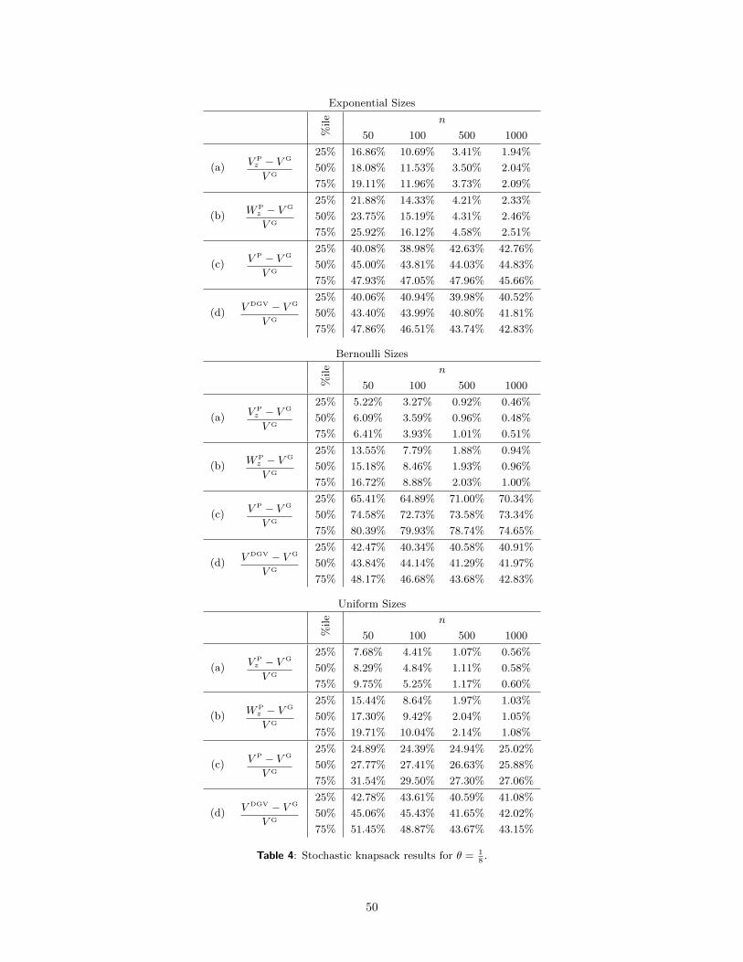
Exponential Sizes

%ile n

50 100 500 1000

(a)V Pz − V G

V G

25% 16.86% 10.69% 3.41% 1.94%

50% 18.08% 11.53% 3.50% 2.04%

75% 19.11% 11.96% 3.73% 2.09%

(b)WP

z − V G

V G

25% 21.88% 14.33% 4.21% 2.33%

50% 23.75% 15.19% 4.31% 2.46%

75% 25.92% 16.12% 4.58% 2.51%

(c)V P − V G

V G

25% 40.08% 38.98% 42.63% 42.76%

50% 45.00% 43.81% 44.03% 44.83%

75% 47.93% 47.05% 47.96% 45.66%

(d)V DGV − V G

V G

25% 40.06% 40.94% 39.98% 40.52%

50% 43.40% 43.99% 40.80% 41.81%

75% 47.86% 46.51% 43.74% 42.83%

Bernoulli Sizes

%ile n

50 100 500 1000

(a)V Pz − V G

V G

25% 5.22% 3.27% 0.92% 0.46%

50% 6.09% 3.59% 0.96% 0.48%

75% 6.41% 3.93% 1.01% 0.51%

(b)WP

z − V G

V G

25% 13.55% 7.79% 1.88% 0.94%

50% 15.18% 8.46% 1.93% 0.96%

75% 16.72% 8.88% 2.03% 1.00%

(c)V P − V G

V G

25% 65.41% 64.89% 71.00% 70.34%

50% 74.58% 72.73% 73.58% 73.34%

75% 80.39% 79.93% 78.74% 74.65%

(d)V DGV − V G

V G

25% 42.47% 40.34% 40.58% 40.91%

50% 43.84% 44.14% 41.29% 41.97%

75% 48.17% 46.68% 43.68% 42.83%

Uniform Sizes

%ile n

50 100 500 1000

(a)V Pz − V G

V G

25% 7.68% 4.41% 1.07% 0.56%

50% 8.29% 4.84% 1.11% 0.58%

75% 9.75% 5.25% 1.17% 0.60%

(b)WP

z − V G

V G

25% 15.44% 8.64% 1.97% 1.03%

50% 17.30% 9.42% 2.04% 1.05%

75% 19.71% 10.04% 2.14% 1.08%

(c)V P − V G

V G

25% 24.89% 24.39% 24.94% 25.02%

50% 27.77% 27.41% 26.63% 25.88%

75% 31.54% 29.50% 27.30% 27.06%

(d)V DGV − V G

V G

25% 42.78% 43.61% 40.59% 41.08%

50% 45.06% 45.43% 41.65% 42.02%

75% 51.45% 48.87% 43.67% 43.15%

Table 4: Stochastic knapsack results for θ = 18.

50

References

Andersen, L. M. and Broadie, M. (2004), ‘Primal-dual simulation algorithm for pricing multidimensionalamerican options’, Management Science 50, 1222–1234.

Arnold, B., Balakrishnan, N. and Nagaraja, H. (2008), A First Course in Order Statistics, Society forIndustrial and Applied Mathematics.

Aven, T. (1985), ‘Upper (lower) bounds on the mean of the maximum (minimum) of a number of randomvariables’, Journal of Applied Probability 22(3), 723–728.

Blado, D., Hu, W. and Toriello, A. (2015), Semi-infinite relaxations for the dynamic knapsack problem withstochastic item sizes. Working Paper.

Borodin, A. and El-Yaniv, R. (1998), Online Computation and Competitive Analysis, Cambridge UniversityPress, New York, NY, USA.

Brown, D. B. and Haugh, M. B. (2014), Information relaxation bounds for infinite horizon markov decisionprocesses. Working Paper.

Brown, D. B. and Smith, J. E. (2011), ‘Dynamic portfolio optimization with transaction costs: Heuristicsand dual bounds’, Management Science 57(10), 1752–1770.

Brown, D. B. and Smith, J. E. (2014), ‘Information relaxations, duality, and convex stochastic dynamicprograms’, Operations Research 62(6), 1394–1415.

Brown, D. B., Smith, J. E. and Sun, P. (2010), ‘Information relaxations and duality in stochastic dynamicprograms’, Operations Research 58(4-part-1), 785–801.

Childs, P. D. and Triantis, A. J. (1999), ‘Dynamic r&d investment policies’, Management Science45(10), 1359–1377.

de Farias, D. P. and Roy, B. V. (2003), ‘The linear programming approach to approximate dynamic pro-gramming’, Operations Research 51(6), 850–865.

Dean, B. C., Goemans, M. X. and Vondrak, J. (2008), ‘Approximating the stochastic knapsack problem:The benefit of adaptivity’, Mathematics of Operations Research 33(4), 945–964.

Derman, C., Lieberman, C. and Ross, S. (1978), ‘A renewal decision problem’, Management Science24(5), 554–561.

Desai, V., Farias, V. F. and Moallemi, C. C. (2012), ‘Pathwise optimization for optimal stopping problems’,Management Science 58, 2292–2308.

Devalkar, S., Anupindi, R. and Sinha, A. (2011), ‘Integrated optimization of procurement, processing, andtrade of commodities’, Operations Research 59, 1369–1381.

Ding, M. and Eliashberg, J. (2002), ‘Structuring the new product development pipeline’, Management Science48(3), 343–363.

Feldman, J., Henzinger, M., Korula, N., Mirrokni, V. S. and Stein, C. (2010), Online stochastic packingapplied to display ad allocation, in ‘Proceedings of the 18th annual European conference on Algorithms:Part I’, ESA’10, Springer-Verlag, pp. 182–194.

Gallego, G. and van Ryzin, G. (1994), ‘Optimal dynamic pricing of inventories with stochastic demand overfinite horizons’, Management Science 40(8), 999–1020.

Garg, N., Gupta, A., Leonardi, S. and Sankowski, P. (2008), Stochastic analyses for online combinatorialoptimization problems, in ‘Proceedings of the Nineteenth Annual ACM-SIAM Symposium on DiscreteAlgorithms’, SODA ’08, Society for Industrial and Applied Mathematics, pp. 942–951.

51

Grandoni, F., Gupta, A., Leonardi, S., Miettinen, P., Sankowski, P. and Singh, M. (2008), Set coveringwith our eyes closed, in ‘Foundations of Computer Science, 2008. FOCS ’08. IEEE 49th Annual IEEESymposium on’, pp. 347–356.

Hall, L. A., Schulz, A. S., Shmoys, D. B. and Wein, J. (1997), ‘Scheduling to minimize average completiontime: Off-line and on-line approximation algorithms’, Mathematics of Operations Research 22(3), 513–544.

Haugh, M. B., Iyengar, G. and Wang, C. (2014), Tax-aware dynamic asset allocation. Working Paper.

Haugh, M. B. and Kogan, L. (2004), ‘Pricing american options: A duality approach’, Operations Research52, 258–270.

Haugh, M. B. and Lim, A. E. (2012), ‘Linear-quadratic control and information relaxations’, OperationsResearch Letters 40(6), 521–528.

Lai, G., Margot, F. and Secomandi, N. (2010), ‘An approximate dynamic programming approach to bench-mark practice-based heuristics for natural gas storage valuation’, Operations Research 58, 564–582.

Manshadi, V. H., Gharan, S. O. and Saberi, A. (2012), ‘Online stochastic matching: Online actions basedon offline statistics’, Mathematics of Operations Research 37(4), 559–573.

Mohring, R. H., Schulz, A. S. and Uetz, M. (1999), ‘Approximation in stochastic scheduling: The power oflp-based priority policies’, J. ACM 46(6), 924–942.

Nadarajah, S., Margot, F. and Secomandi, N. (2015), ‘Relaxations of approximate linear programs for thereal option management of commodity storage’, Management Science (Articles in Advance) .

Papstavrou, J. D., Rajagopalan, S. and Kleywegt, A. J. (1996), ‘The dynamic and stochastic knapsackproblem with deadlines’, Management Science 42(12), 1706–1718.

Pinedo, M. L. (2012), Scheduling, Springer US.

Rogers, L. (2002), ‘Monte carlo valuation of american options’, Mathematical Finance 12, 271–286.

Rogers, L. (2007), ‘Pathwise stochastic optimal control’, SIAM Journal on Control and Optimization46, 1116–1132.

Rothkopf, M. (1966), ‘Scheduling with random service times’, Management Science 12, 703–713.

Santiago, L. and Vakili, P. (2005), ‘On the value of flexibility in r&d projects’, Management Science51(8), 1206–1218.

Smith, W. (1956), ‘Various optimizers for single-stage production’, Nav. Res. Log. Quarterly 3, 59–66.

Talluri, K. and van Ryzin, G. (1998), ‘An analysis of bid-price controls for network revenue management’,Management Science 44(11), 1577–1593.

Weiss, G. (1990), ‘Approximation results in parallel machines stochastic scheduling’, Annals of OperationsResearch 26(1), 195–242.

Whittle, P. (1988), ‘Restless bandits: Activity allocation in a changing world’, Journal of Applied Probability25, 287–298.

52