PDE Boundary Control for Flexible Articulated

Aircraft Wings

Aditya A. Paranjape�, Soon-Jo Chungy, and Miroslav Krsticz

The paper considers a boundary control formulation for PDEs with a system outputgiven by a spatial integral of weighted functions of the state. This formulation is directlyapplicable to the control of an aircraft with articulated exible wings, in which case theoutput of interest is a net aerodynamic force or moment. Flexible wings can be controlledvia actuation at the root or the tip. The problem of beam twist is analysed in detail toillustrate the formulation, and it shown that the control law ensures that the error betweenthe desired output signal and the actual output signal decreases exponentially to an uniformultimate bound. Stability of the closed loop system is proved by Lyapunov techniques. Theformulation is demonstrated by simulations.

Nomenclature

c wing chord length

E; G elastic modulus and shear modulus of the wing material

g gravitational constant

Iyy; J second moment of area of the airfoil and torsion constant

m; Ip mass per unit length of the wing, airfoil second moment of inertia

V ight speed

xa; xe non-dimensional distance of aerodynamic center and airfoil center of mass

from shear center

�R; �R bending slope (dihedral) and incidence angle at the wing root

� Kelvin-Voigt damping coe�cient

� twist angle

� bending displacemnt

Notation

t; y time and spanwise spatial variable

vt; vy@v

@tand

@v

@y

vtyy@3v

@t@y2(and so on)

_v time derivative of a variable v(t)

I. Introduction

A new concept for controlling micro aerial vehicles, based on wing articulation, was introduced in Refs. [1,2]. The concept lends itself readily to aeroelastic tailoring. Aeroelastic tailoring is seen as an asset in the

�Doctoral candidate, Department of Aerospace Engineering, Univ. of Illinois at Urbana-Champaign (UIUC), Urbana, IL.Email: paranja2@illinois.edu; Student Member, AIAA.yAssistant Professor, Department of Aerospace Engineering, University of Illinois at Urbana-Champaign Email:

sjchung@illinois.edu; Senior Member, AIAA.zDaniel L. Alspach Professor of Dynamic Systems and Control, Dept. of Mechanical and Aerospace Engineering, Univ. of

California, San Diego, La Jolla, CA 92903. Email: krstic@ucsd.edu.

1 of 15

American Institute of Aeronautics and Astronautics

AIAA Guidance, Navigation, and Control Conference08 - 11 August 2011, Portland, Oregon

AIAA 2011-6486

Copyright © 2011 by Aditya A. Paranjape, Soon-Jo Chung and Miroslav Krstic. Published by the American Institute of Aeronautics and Astronautics, Inc., with permission.

Dow

nloa

ded

by U

NIV

ER

SIT

Y O

F IL

LIN

OIS

on

Mar

ch 2

0, 2

013

| http

://ar

c.ai

aa.o

rg |

DO

I: 1

0.25

14/6

.201

1-64

86

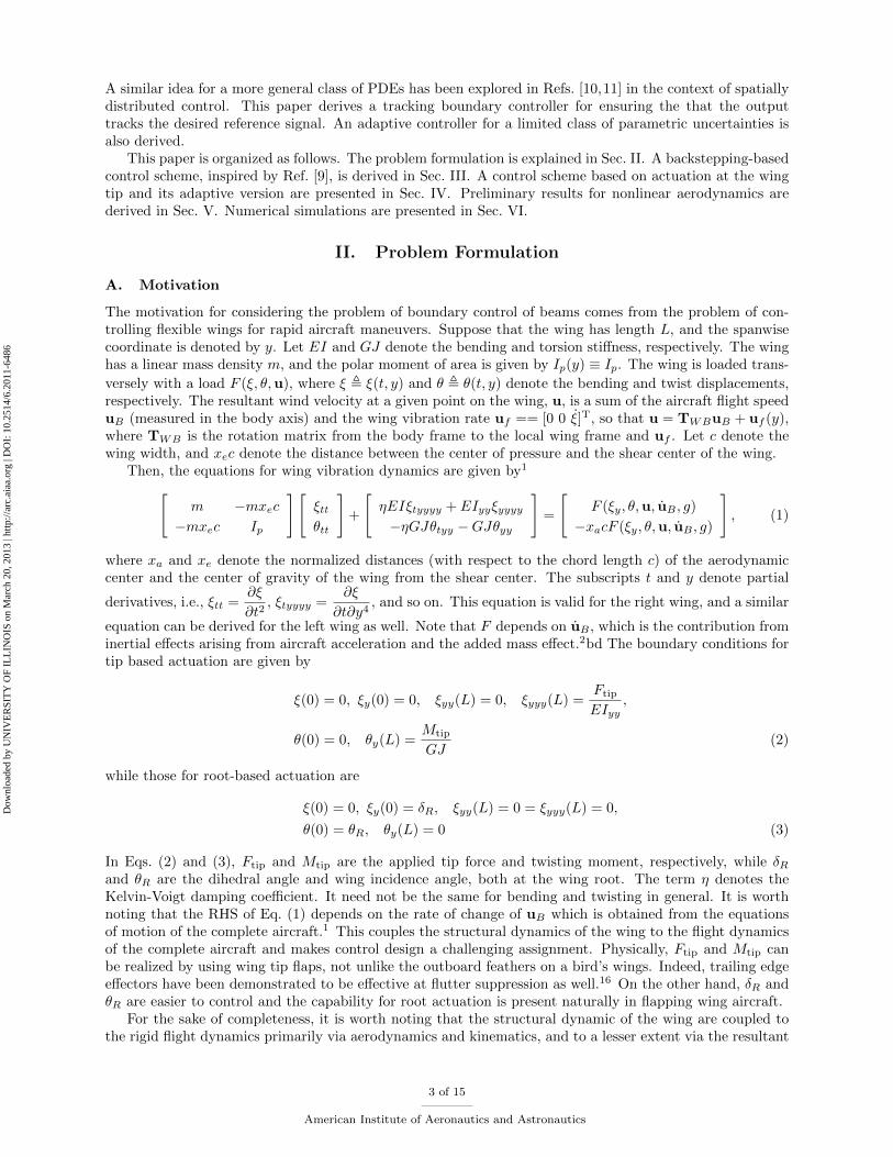
(a) Root actuation (b) Tip actuation

Figure 1. A schematic showing an MAV with highly exible wings controlled at the wing root and wing tip,respectively.

development of agile micro aerial vehicles.1,3{5 Wing exibility not only improves aircraft performance andstability passively, but can also be actuated actively for control.1,3, 6 Figure 1 shows a conceptual MAV withhighly exible wings whose deformation can be controlled actively by actuators located at the wing rootand/or the wing tip.

Broadly speaking, continuous systems such as wings can be controlled in two ways: distributed control andboundary control. The former approach relies on a series or a network of actuators and sensors distributedover the system. The latter approach relies on actuators deployed only on the boundary of the system underconsideration. For practical engineering applications, the most important bene�t of boundary control is thereduction in the number of actuators. Consider, for example, a exible wing mounted on a miniature aircraft.This example is illustrative of the reverse engineering of bird ight. Whereas feathers distributed all overthe wing are known to play an active role in ight control, installing such a distributed scheme would incursubstantial penalties in weight as well as costs. The bene�ts of distributed actuation can be made up, in part,by a combination of good design and sound boundary control. This paper presents a boundary control (BC)problem for wing twist which could be extended to a wider class of hyperbolic partial di�erential equations(PDEs).

There is a substantial amount of literature on boundary control theory of PDEs (see Ref. [7{12] formaterial pertinent to this paper and the references cited therein). There are two sets of methods for boundarycontrol of PDEs. The �rst approach involves converting the PDEs into ordinary di�erential equations usingapproximation methods such as those of Galerkin or Rayleigh-Ritz.11,13 This renders the problem amenableto control by any of a large number of linear and nonlinear methods for control of systems described byODEs.13 The second approach involves keeping the PDEs intact, and using a \model-following" approachas described in a recent book by Krstic and Smyshlyaev.9 In particular, this approach seeks to achieve an apriori prescribed deformation. This is indeed the objective of problems such as maneuvering robotic arms9,14

or suppressing vibrations in a exible beam.15 On the other hand, in problems such as those involving exibleaircraft wings where the control objective would be to achieve a net aerodynamic force or moment, therecould be several candidate deformations. Prescribing one particular candidate deformation places a greaterdemand on the control system.

It is worth noting that if a PDE is approximated by Galerkin’s method, the problem of achieving an inte-gral objective reduces to a standard output control problem. Whereas solutions to output control problemsin an ODE setting are abundantly known, an ODE-based approximation to PDEs usually results in systemshaving large orders. It is not very easy to incorporate a time-varying boundary condition into the basis func-tions which results in the possibility that the control design process becomes tedious and the control lawsnon-intuitive. Ref. [10] also points out that a �nite-state approximation may wrongly render fundamentalsystem theoretic properties like controllability and observability to be functions of the approximation.

In this paper, the control objective is restricted to achieving the net aerodynamic force or moment, anabstraction of which is ensuring that some weighted integral of the deformation equals the prescribed value.

2 of 15

American Institute of Aeronautics and Astronautics

Dow

nloa

ded

by U

NIV

ER

SIT

Y O

F IL

LIN

OIS

on

Mar

ch 2

0, 2

013

| http

://ar

c.ai

aa.o

rg |

DO

I: 1

0.25

14/6

.201

1-64

86

A similar idea for a more general class of PDEs has been explored in Refs. [10,11] in the context of spatiallydistributed control. This paper derives a tracking boundary controller for ensuring the that the outputtracks the desired reference signal. An adaptive controller for a limited class of parametric uncertainties isalso derived.

This paper is organized as follows. The problem formulation is explained in Sec. II. A backstepping-basedcontrol scheme, inspired by Ref. [9], is derived in Sec. III. A control scheme based on actuation at the wingtip and its adaptive version are presented in Sec. IV. Preliminary results for nonlinear aerodynamics arederived in Sec. V. Numerical simulations are presented in Sec. VI.

II. Problem Formulation

A. Motivation

The motivation for considering the problem of boundary control of beams comes from the problem of con-trolling exible wings for rapid aircraft maneuvers. Suppose that the wing has length L, and the spanwisecoordinate is denoted by y. Let EI and GJ denote the bending and torsion sti�ness, respectively. The winghas a linear mass density m, and the polar moment of area is given by Ip(y) � Ip. The wing is loaded trans-

versely with a load F (�; �;u), where � , �(t; y) and � , �(t; y) denote the bending and twist displacements,respectively. The resultant wind velocity at a given point on the wing, u, is a sum of the aircraft ight speeduB (measured in the body axis) and the wing vibration rate uf == [0 0 _�]T, so that u = TWBuB + uf (y),where TWB is the rotation matrix from the body frame to the local wing frame and uf . Let c denote thewing width, and xec denote the distance between the center of pressure and the shear center of the wing.

Then, the equations for wing vibration dynamics are given by1"m �mxec

�mxec Ip

#"�tt

�tt

#+

"�EI�tyyyy + EIyy�yyyy

��GJ�tyy �GJ�yy

#=

"F (�y; �;u; _uB ; g)

�xacF (�y; �;u; _uB ; g)

#; (1)

where xa and xe denote the normalized distances (with respect to the chord length c) of the aerodynamiccenter and the center of gravity of the wing from the shear center. The subscripts t and y denote partial

derivatives, i.e., �tt =@�

@t2, �tyyyy =

@�

@t@y4, and so on. This equation is valid for the right wing, and a similar

equation can be derived for the left wing as well. Note that F depends on _uB , which is the contribution frominertial e�ects arising from aircraft acceleration and the added mass e�ect.2bd The boundary conditions fortip based actuation are given by

�(0) = 0; �y(0) = 0; �yy(L) = 0; �yyy(L) =Ftip

EIyy;

�(0) = 0; �y(L) =Mtip

GJ(2)

while those for root-based actuation are

�(0) = 0; �y(0) = �R; �yy(L) = 0 = �yyy(L) = 0;

�(0) = �R; �y(L) = 0 (3)

In Eqs. (2) and (3), Ftip and Mtip are the applied tip force and twisting moment, respectively, while �Rand �R are the dihedral angle and wing incidence angle, both at the wing root. The term � denotes theKelvin-Voigt damping coe�cient. It need not be the same for bending and twisting in general. It is worthnoting that the RHS of Eq. (1) depends on the rate of change of uB which is obtained from the equationsof motion of the complete aircraft.1 This couples the structural dynamics of the wing to the ight dynamicsof the complete aircraft and makes control design a challenging assignment. Physically, Ftip and Mtip canbe realized by using wing tip aps, not unlike the outboard feathers on a bird’s wings. Indeed, trailing edgee�ectors have been demonstrated to be e�ective at utter suppression as well.16 On the other hand, �R and�R are easier to control and the capability for root actuation is present naturally in apping wing aircraft.

For the sake of completeness, it is worth noting that the structural dynamic of the wing are coupled tothe rigid ight dynamics primarily via aerodynamics and kinematics, and to a lesser extent via the resultant

3 of 15

American Institute of Aeronautics and Astronautics

Dow

nloa

ded

by U

NIV

ER

SIT

Y O

F IL

LIN

OIS

on

Mar

ch 2

0, 2

013

| http

://ar

c.ai

aa.o

rg |

DO

I: 1

0.25

14/6

.201

1-64

86

variation in mass distribution. The coupled equations of motion have the following structure:

m( _uB + S(!B)uB) + ~m

Zw

( _uf + S(!B)uf )dy = Fnet

J _!B + S(!B)J!B +

Zw

(Ip(y) _!f + S(!B)Ip(y)!f )) dy = Mnet

where:Rw

denotes integration over the wing, and Fnet and Mnet represent the net external (aerodynamic +

gravitational) force and moment on the aircraft. Furthermore, !B and !f = [0 _� 0]T are vector representa-tions of the aircraft angular velocity and the twist rate of the wing, with components in the aircraft bodyaxes. The reader is referred to Ref. [1] for a detailed and more general derivation of the equations of motion.

B. Problem Considered in this Paper

Control methodology in this paper is developed systematically for a simple linear case with just the twistdegree of freedom. Therefore, only the second equation in Eq. (1) is relevant to this paper. This is aconsiderable simpli�cation, but it provides most of the necessary ingredients to design a controller for thecomplete system. The control objective is to ensure that

limt!1

Z L

0

�(t; y)dy �H(t)

!= 0 (4)

where H(t) is a su�ciently smooth time-varying signal. Physically, the left hand side could be taken tocommand, for example, a desired value of the lift. In a linear setting, the net lift produced by the wing

is given byR L0

0:5�V 2cCl;��, where � is the air density and Cl;� is the lift curve slope (measured per unitspan of the wing). Depending on the aerodynamic theory, the left hand side of the above equation may bea nonlinear function of �. It is almost always a function of y, and a solution to this case is presented later inthe paper. It may be possible to treat the aircraft speed and angular rates as disturbances while designinga controller for the wing structural dynamics, but this point needs further investigation.

III. Boundary Control of Twisting Motion: Root Control

Consider the case where the exible wing needs to be controlled from the wing root, i.e., the PDE forwing twist is given by

�tt � b�tyy � a�yy = M�;

�y(L) = 0; �(0) = U(t) : : :wing tip free, root displacement controlled (5)

where a = GJ=Ip, b = �a, and M� = �xacF=Ip in Eq. (1). The net force, F , has been assumed to be linearin �. It is easy to check that the system has an in�nite relative degree with respect to the output in Eq. (4).Thus, one needs to approach this problem in two steps. In the �rst step, the desired steady state responseis determined. In the second step, the error dynamics between the system behavior and the desired steadystate are stabilized using backstepping.9 Therefore, the control U(t) may be decomposed into two parts

U(t) = Ud(t) + u(t); (6)

where Ud is the desired boundary condition at the wing root for which the integral objective, Eq. (4), issatis�ed, while u(t) is the stabilizing controller obtained from backstepping.

A. Boundary Condition for the Desired Dynamics

If the desired behavior is an equilibrium (i.e., H(t) � H), then the steady state PDE is given by

�d;yy + �2�d = 0; �d;y(L) = 0; �d(0) = Ud (7)

where �2 = M=a and the subscript, d, denotes the desired (also, in this case, steady) state. The followingcontrol law, Ud, ensures that the condition Eq. (4) is satis�ed.

Ud =�H

tan(�L)(8)

4 of 15

American Institute of Aeronautics and Astronautics

Dow

nloa

ded

by U

NIV

ER

SIT

Y O

F IL

LIN

OIS

on

Mar

ch 2

0, 2

013

| http

://ar

c.ai

aa.o

rg |

DO

I: 1

0.25

14/6

.201

1-64

86

Alternatively, the desired behavior may be time varying in which case the boundary condition prescribedat the root needs to be determined separately. The boundary condition at the wing tip, on the other hand,is relatively easy to choose because, as shown in Sec. IV, the system has a relative degree of 2 for the outputin Eq. (4) and the wing tip moment as the control input.

B. Backstepping

Backstepping is carried out in two steps: (a) Target dynamics are identi�ed, and (b) a backstepping trans-formation converts the system dynamics (in this case, the error dynamics) into the target dynamics and theu(t) is obtained in the process. The method described by Krstic and Smyshlyaev9 is used here. Let z denotethe error between the system state and the desired steady state value.

Next, consider the target dynamics given by

vtt � bvtyy � avyy = (M � ap)v � bpvt;v(0) = vy(L) = 0 (9)

Using the method of separation of variables, it is easy to check that the eigenvalues of this system are thesolutions of

�2 + b(�2 + p)�+ (a(�2 + p)�M) = 0

where � =2n+ 1

2

�

L; n = 0; ; 1; 2; : : : (10)

The target dynamics are stable if and only if the control design parameter, p, satis�es

p >M

a� �2

4L2(11)

A dummy spatial variable x is introduced and the backstepping transformation between z = � � �d (theerror between the actual dynamics and the desired steady state in Eq. (9)) and v (the target dynamics forthe error state) is given by

v(t; y) = z(t; y)�Z y

L

k(y; x)z(t; x)dx (12)

It is helpful to recall that the z dynamics are given by

ztt � bztyy � azyy = Mz; z(0) = u; zy(L) = 0 (13)

In order to solve for k(x; y), substitute Eqs. (12) and (13) into Eq. (9). Next, isolating the coe�cients of vand vt, the following Klein - Gordon PDE for k(y; x) is derived9

kxx(y; x)� kyy(y; x) = �pk(y; x)

k(y; y) =p

2(L� y); kx(y; L) = 0 (14)

The control input is given by

u(t) = z(t; 0) = �Z L

0

k(0; x)z(x)dx (15)

It remains to explain the derivation of k(x; y). First, we derive expressions for vtt and vyy.

vtt = ztt �Z y

L

k(y; x)ztt(x)dx

= bztyy + azyy +Mz �Z y

L

k(y; x) (bztxx + azxx +Mz) dx

= bztyy + azyy +Mz �Z y

L

k(y; x)Mzdx�Z y

L

kxx(y; x) (bzt(x) + az(x)) dx

�k(y; y)(bzty(y) + azy(y)) + kx(y; y)(bzt(y) + az(y))� kx(y; L)(bzt(L) + az(L)) (16)

5 of 15

American Institute of Aeronautics and Astronautics

Dow

nloa

ded

by U

NIV

ER

SIT

Y O

F IL

LIN

OIS

on

Mar

ch 2

0, 2

013

| http

://ar

c.ai

aa.o

rg |

DO

I: 1

0.25

14/6

.201

1-64

86

The expression for vyy can be derived as follows:

vy = zy(y)� k(y; y)z(y)�Z y

L

ky(y; x)z(x)dx

vyy = zyy(y)� 2ky(y; y)z(y)� kx(y; y)z(y)� k(y; y)zy(y)�Z y

L

kyy(y; x)z(x)dx (17)

The expression for vtyy is similar to that for vyy. Substitute Eqs. (16) and (17) into Eq. (9) and isolate thecoe�cients of z, zy, and z and zy in the integrand. This yields the PDE kxx � kyy = �pk and one of the

two boundary conditions, viz., kx(y; L) = 0. It also yields the condition k(y; y) =p

2y + constant. From the

�rst equation of (17), it follows that k(L;L) = 0 since zy(L) = vy(L) = 0. Therefore, k(y; y) =p

2(L � y),

which is the second boundary condition.One can solve for k(y; x) using successive approximations, as described in Ref.9 Alternately, under the

transformation of coordinates x 7! L�x and y 7! L�y, the BVP in Eq. (14) is identical to the one describedby Krstic and Smyshlyaev.9 The solution is given in terms of the modi�ed Bessel function I1:

k(y; x) = �p2

(L� y)I1(pp((L� y)2 � (L� x)2))pp((L� y)2 � (L� x)2))

(18)

In summary, the control signal, U(t), is given by Eqs. (6), (15) and (18).

C. Discussion

A few observations are worth noting here.

1. The procedure described in the previous subsection is called backstepping because the Volterra operatorin Eq. (12) has a lower triangular structure similar to backstepping transforms for ordinary di�erentialequations. It is a continuum analogue of the backstepping transformations in ODEs and allows thecontroller acting at the boundary to compensate for the undesired (unmatched) dynamics.

2. If the wing is reasonably sti�

�MIpGJ

=M

a<

�2

4L2

�, i.e., GJ > 4L2MIp=�

2, the system can be stabi-

lized with p = 0, i.e., with no additional control input.

3. For stability, it is essential that b > 0, and the Kelvin-Voigt damping coe�cient is always positive. Anegative damping could be introduced due to aerodynamics, but it can be compensated by the termbpvt and wing utter can be prevented. The compensation in damping imposes an additional constrainton p.

4. The controller in Eq. (15) requires that the twist angle at all points on the wing be known. Thisdi�culty can be circumvented by designing a PDE-based observer9 or, practically, using a series ofdistributed sensors and �tting their output with an a priori designed spline.

Recall the observation that for a \su�ciently" sti� wing, no additional stabilizing controller is required.As an illustration, consider the wing of a micro aerial vehicle (MAV). For such wings, a � O(E) > O(107),where E is the Young’s modulus. Furthermore, M � 0:06V 2c2=Ip, where Ip � 10�3�c4 is the second momentof area of the cross section whose thickness is assumed to be 1% of the chord length (a very conservative

estimate). In such cases, M � O(5�105). Therefore,M

a� O(0:05). On the other hand, with L2 � 0:16 (an

aspect ratio of 8, too generous for most MAV!),�2

4L2� 12. Therefore, a typical MAV wing is sti� enough

to be stable in the open loop. On the other hand, one would expect large wings ying at high speeds toexperience loss of stability in the open loop - a phenomenon called wing divergence.

IV. Boundary Control of Twisting Motion: Wing Tip Control

Although backstepping can be employed when the twisting moment at the wing tip is used as the controlinput, it turns out that there is a simpler alternative, as described in this section. It relies on the fact thatthe output has a �nite relative degree with respect to the twisting moment.

6 of 15

American Institute of Aeronautics and Astronautics

Dow

nloa

ded

by U

NIV

ER

SIT

Y O

F IL

LIN

OIS

on

Mar

ch 2

0, 2

013

| http

://ar

c.ai

aa.o

rg |

DO

I: 1

0.25

14/6

.201

1-64

86

A. Tip Boundary Control when All Parameters are Known

As in the previous section, one can design a backstepping controller for the case where a control moment isapplied to the free end (y = L) of the wing while the other end (y = 0) is clamped. In fact, the procedure inboth cases is identical, although the �nal expressions for the control law di�er slightly. Alternately, insofaras MAV are concerned, one may do without a stabilizing controller. The \tracking half" of the controller(Ud(t) in Eq. (6)) may be designed using the output measurements. This method is useful for adaptivedesigns as well. We consider the wing model

�tt � b�tyy � a�yy = M�; a > 0; (19)

where the control input is a moment applied at the wing tip, u(t) = �y(L; t), and b = �a = �GJ=Ip. Thecontrol objective could be assumed to be linear in � because it is usually the total aerodynamic force ormoment produced by the wing. It reduces to the formZ L

0

�(t; y)dy = H(t): (20)

The problem will be solved using a linear control approach. Let e(t) =R L0�(t; y)dy � H(t) denote the

error which needs to be regulated. Then,

�e =

Z L

0

�tt(t; y)dy � �H(t)

=

Z L

0

(a�yy + b�tyy +M�) dy � �H(t)

= a�y(L)� a�y(0) + b�ty(L)� b�ty(0) +Me(t)� �H(t) +MH(t)

= b _u(t) + au(t)� a�y(0)� b�ty(0) +Me(t)� �H(t) +MH(t) (21)

A dynamic controller of the form

b _u(t) + au(t) = �H(t)�MH(t)� (M + k)e(t)� kc _e(t) + a�y(0) + b�ty(0) (22)

renders the system into the spring-mass form

�e(t) + kc _e(t) + ke(t) = 0: (23)

The control law in Eq. (22) is similar to internal model-based controllers and so much would be expectedgiven that it does not rely on full state feedback. In fact, it suggests that � need not be monitored ormeasured at all locations on the wing. Instead, only �y(0) needs to be measured or estimated. The referencesignal H(t) is known. It may be di�cult to inject damping, _e(t). This is because _e(t) is the rate of changeof the lift and in practice, would require di�erentiating noisy acceleration signals.

Another interesting observation is that although the PDE system had an in�nite relative degree whenthe root twist was chosen as the control input, the relative degree is 2 when twisting moment at the wing tipis considered as the input. This facilitates the control law design in this section considerably. The controllaw design described is this section lends itself readily to adaptation should a and/or M be unknown. In thecontrol law (22), a and M could be readily replaced by the corresponding estimated values obtained from apassive estimator.

Finally, if �(0) as well as �y(L) can be controlled, it may be possible to ensure that the wing deformationproduces the desired net lift as well as moment. This control scheme is physically realizable in MAVs. Forexample, apping wing MAVs such as the robotic bat described in Ref. [17] has a twist angle actuator atthe root. A small ap at the wing tip, not unlike the outboard feathers in a bird wing, can provide twistingmoment at the tip.

B. Adaptive Control

Adaptive control is a useful method when system dynamics and/or parameters are unknown. The elasticproperties of a linearly elastic structure can be characterized experimentally. The aerodynamic force and mo-ment distribution would be usually hard to characterize or if characterized at all, would show a considerably

7 of 15

American Institute of Aeronautics and Astronautics

Dow

nloa

ded

by U

NIV

ER

SIT

Y O

F IL

LIN

OIS

on

Mar

ch 2

0, 2

013

| http

://ar

c.ai

aa.o

rg |

DO

I: 1

0.25

14/6

.201

1-64

86

nonlinear spatial distribution. For example, a simple rectangular wing has an elliptic lift distribution undernominal ight conditions.18 Nonlinearities would be considered in a later section of this paper. Consider thecase where M is constant, but unknown. This is not a very realistic model, but provides a sound foundationto design an adaptive controller.

Consider the dynamics in Eq. (19) with the objective in Eq. (20). The control law in (22) is modi�ed sothat

b _u(t) + au(t) = �H(t)� M̂(t)(H(t) + e(t))� ke(t)� kc _e(t) + a�y(0) + b�ty(0) (24)

where M̂(t) is the estimated value of M . The error dynamics are given by

�e(t) + kc _e(t) + ke(t) = � ~M(t)(H(t) + e(t)); (25)

where ~M(t) = M̂(t)�M(t). An adaptive law must be designed for M̂(t) to ensure that the error, e(t), goesto zero asymptotically.

For notational convenience, de�ne x = [e(t); _e(t)]T and A =

"0 1

�k �kc

#. Since A is Hurwitz, it follows

that there exists a positive de�nite symmetric matrix P = PT > 0 satisfying the Lyapunov equation

PA+ATP = �I; (26)

where I is the 2 � 2 identity matrix. We assume that jM(t)j is bounded above by B1 and j _M(t)j by B2,where B1 and B2 are constants.

Consider the Lyapunov function

V (t) = xT(t)Px(t) +1

~M(t)2; (27)

where > 0 is the adaptive gain. Di�erentiating both sides with respect to t, we get

_V (t) = �xT(t)x(t) +2

~M(t)

_̂M(t)� xTP

"0

1

#(e(t) +H)� _M(t)

!(28)

With the adaptive law

_̂M(t) = Proj

M̂(t); xTP

"0

1

#(e(t) +H)

!(29)

it follows that

_V (t) � �xT(t)x(t)� 2

~M(t) _M(t) � �1

�max(P )

�xTPx+

1

~M(t)2

�+

4B21

�max(P )+

4B1B2

(30)

The projection law can be chosen so that jM̂(t)j < B1 (the same bound as that on M(t)). Therefore, itfollows that

_V (t) � �1

�max(P )(1� �b)V (t) 8 V (t) >

4�max(P )B1B2 + 4B21

�b ; �b 2 (0; 1) (31)

and hence, the solution is uniformly ultimately bounded with some T � 0 and with the ultimate boundgiven by

kx(t)k1 � kx(t)k2 �

s4�max(P )B1B2 + 4B2

1

�min(P )�b 8 t � T (32)

where �b 2 (0; 1). Note that the bound on kx(t)k1 can be made arbitarily small by choosing a large . Thesteady state beam shape of the wing depends on the steady state value of the error ~M(t). Finally, it is worthnoting that although a and b were assumed to be known, the aforementioned analysis can be repeated toaccommodate an unknown a and b as well.

8 of 15

American Institute of Aeronautics and Astronautics

Dow

nloa

ded

by U

NIV

ER

SIT

Y O

F IL

LIN

OIS

on

Mar

ch 2

0, 2

013

| http

://ar

c.ai

aa.o

rg |

DO

I: 1

0.25

14/6

.201

1-64

86

V. Nonlinearities

Two cases are presented in this section. The �rst case concerns a nonlinear twisting moment function.This problem is addressed via linearization. The second case considers a twisting moment which is linear inthe twist angle, but with a spatially varying coe�cient. The second problem is addressed using backstepping.

For brevity, only root actuation has been considered in this section. The analysis can be extended toactuation at the wing tip with minimal e�ort.

A. Local Linear Analysis

A nonlinear problem which is of interest to the present discussion would be to regulate a PDE of the form

�tt � b�tyy � a�yy = �xacF (�; �t); �y(L) = 0; �(0) = U(t) (33)

where xa is the normalized (with respect to the chord length c) distance between the shear center and theaerodynamic center of the wing. The nonlinearity on the RHS arises from the inclusion of �t in the local ow velocity, and is widely used, for e.g., in utter prediction.13 As in the earlier part of the paper, considerthe error dynamics between the actual system and the steady state.

Desired: �tt � b�tyy � a�yy = �xacF (�; �t); �y(L) = 0; �(0) = Ud(t)

Error Dynamics: ett � betyy � aeyy = �xacF (�; �t)�M(�ss; 0); ey(L) = 0; e(0) = u(t) (34)

where the subscript ‘ss’ has been used to denote the steady state. Notice that, on this occasion, we have nosimple expression for Ud. Instead, it must be calculated on a case-by-case basis for di�erent nonlinearitieson the right hand side. The nonlinear term can be approximated to the �rst order to get

ett � betyy � aeyy = M2et +M1e; ey(L) = 0; e(0) = u(t) (35)

where the coe�cients M1 = �xac@F (�; �t)

@�and M2 = �xac

@F (�; �t)

@�tdepend on the steady state �.

Consider the following target dynamics for backstepping:

vtt � bvtyy � avyy = M2vt +M1v � apv � bpvt;v(0) = vy(L) = 0 (36)

The characteristic equation is given by

�2 + (b�2 + bp�M2)�+ (a(�2 + p)�M1) = 0 (37)

where �2 =�2

4L2. The target dynamics are stable if and only if

p > max

��M1

a� �2

�;

�M2

b� �2

��(38)

The rest of the backstepping transformation is identical to that described in Section III-B.

B. Lyapunov-based Analysis for Spatially-Varying M(y)

In this section, we show that backstepping, described in Section III-B, can be used to control nonlinearsystems of the form

�tt(t; y)� b�tyy � a�yy = M(y)�; �y(L) = 0; �(0) = U(t) = u(t) (39)

where M(y) > 0 represents the moment distribution on the wing and is a function of the wing geometry.Physically, it captures the e�ect of downwash on a �nite wing.18 There is no loss of generality, as one mayinfer from the analysis in Sec. III-B, in setting Ud(t) = 0, which implies that U(t) = u(t). The problem oftracking reduces to one of regulation. Stability analysis is completed in three steps:

9 of 15

American Institute of Aeronautics and Astronautics

Dow

nloa

ded

by U

NIV

ER

SIT

Y O

F IL

LIN

OIS

on

Mar

ch 2

0, 2

013

| http

://ar

c.ai

aa.o

rg |

DO

I: 1

0.25

14/6

.201

1-64

86

1. First, the backstepping transformation in Eqs. (12) and (14) is invoked to transform the system dy-namics into \target" dynamics (see Eq. (40)).

2. The target dynamics are decomposed into \nominal" dynamics and a vanishing perturbation.

3. The nominal dynamics are shown to be exponentially stable, which implies that there exists a class offunctions M(y) for which the target system is exponentially stable.

The �rst step is to identify the target dynamics. Using the backstepping transformation (12), (14) and(18), i.e.,

v(t; y) = �(t; y)�Z y

L

k(y; x)�(t; x)dx;

k(y; x) = �p2

(L� y)I1(pp((L� y)2 � (L� x)2))pp((L� y)2 � (L� x)2))

;

we obtain the target dynamics

vtt(y)� bvtyy � avyy � (M(y)� ap)v + bpvt = M(y)

Z y

L

k(y; x)�(x)dx�Z y

L

k(y; x)M(x)�(x)dx;

=

Z y

L

M 0(x)

Z x

L

k(y; z)�(z)dzdx , �(x)

v(0) = v0(L) = 0; p > maxy

M(y)

a(40)

The RHS of Eq. (40) may be viewed as a perturbation. The bound on the RHS is calculated as follows:

�(y) �

maxy

Z L

0

jk(y; z)�(z)jdz

! Z L

0

jM 0(x)jdx

!

�

Z L

0

jM 0(x)jdx

!0@maxy

sZ L

0

k(y; z)2dz

1A0@sZ L

0

�(z)2dz

1A = K1k�k (41)

where the constantK1 is a (known) bound on�R L

0jM 0(x)jdx

��maxy

qR L0k(y; z)2dz

�and k�k =

qR L0�(z)2dz

(the norm of �). Furthermore, as shown in Ref. [9], there exists a bounded function l(x; y) such that

�(t; y) = v(t; y)�Z y

L

l(y; x)v(t; x)dx;

=) k�k � K2kvk; (42)

where K2 is another known constant. Hence, from Eqs. (41) and (42), it follows that

�(x) � K1K2kvk (43)

Hence, the perturbation on the RHS of Eq. (40) is vanishing in v.Next, we prove the exponential stability of the nominal dynamics given by

vtt(y)� bvtyy � avyy = (M(y)� ap)v � bpvt; v(0) = v0(L) = 0; p > maxy

M(y)

a(44)

In order to show stability, consider the Lyapunov function

V (t) =

Z L

0

v2t2

+av2y2

+ (ap�M(y))v2

2+ �vvt

!dy (45)

10 of 15

American Institute of Aeronautics and Astronautics

Dow

nloa

ded

by U

NIV

ER

SIT

Y O

F IL

LIN

OIS

on

Mar

ch 2

0, 2

013

| http

://ar

c.ai

aa.o

rg |

DO

I: 1

0.25

14/6

.201

1-64

86

The above Lyapunov function is positive de�nite for a large enough p > maxyM(y)

aand small enough � > 0.

A bound for � will be derived presently. Di�erentiating V (t) with respect to t yields

_V (t) =

Z L

0

�vtvtt + avyvty + (ap�M(y))vvt + �v2t + �vvtt

�(46)

The �rst term in the integrand can be expanded, followed by integration by parts, so thatZ L

0

vtvttdy =

Z L

0

�bvtyyvt + avyyvt � (ap�M(y))vvt � bpv2t

�dy

=

Z L

0

��bv2ty � avyvty � (ap�M(y))vvt � bpv2t

�dy (47)

A similar expression can be calculated forR L0�vvttdy. Substituting Eq. (47) into (46), it follows that

_V (t) =

Z L

0

�(�bp+ �)v2t � bv2ty � a�v2y � (ap�M(y))�v2

�dy +

Z L

0

(�bvvtyy � �bpvvt) dy

Since v(0) = vy(L) = 0, it follows that

_V (t) =

Z L

0

�(�bp+ �)v2t � bv2ty � a�v2y � (ap�M(y))�v2

�dy +

Z L

0

(��bvyvty � �bpvvt) dy (48)

Using Young’s and Cauchy-Schwarz inequalities, it follows thatZ L

0

(��bvyvty � �bpvvt) dy ��b

2

Z L

0

�v2y +

v2ty�

!dy +

�bp

2

Z L

0

��v2 +

v2t�

�dy (49)

Therefore,

_V (t) �Z L

0

���bp+ � +

pb

2

�v2t �

b

2v2ty � (a� 0:5�b)�v2y �

�ap�M(y)� �pb

2

��v2�dy

If � is chosen such that

� < min

�1;

(b� 2�)p

2;

2(ap�M(y)� �p)bp

�8 y � L (50)

where � is another small number such that � < min (a�M(y)=p; b) 8y � L, then it follows that

_V � ���2V (51)

This proves exponential stability and limt!1 v = 0. Note that the condition p > maxyM(y)

a+� is stronger

than the condition obtained for linear systems. Increasing p allows us to choose a larger �, subject to theconstraint arising from b, to improve the guaranteed rate of convergence. Furthermore, since � does notappear in the control law, it does not have any bearing on the performance and stability of the actualsystem.

The nominal system has been shown to be exponentially stable. Furthermore, the perturbation on theRHS of Eq. (40) is vanishing in v, as shown in Eq. (43). Hence, it follows that the nominal system is robust

to su�ciently small perturbations. In particular, it is exponentially stable for su�ciently smallR L0jM 0(y)jdy

(e.g., see Lemma 9.1 in Khalil19 for an ODE analogue), i.e., for a su�ciently small K1 in Eq. (41).A theoretical bound on K1 can be calculated by noting that, had we retained the perturbation term

�(y) ,R yLM 0(x)

R xLk(y; z)�(z)dzdx, it would have entered _V (t) via terms involving vtt in Eq. (48). Using

the Cauchy-Schwarz inequality, it can be shown that the change in _V (t) arising from the inclusion of �(y)is given by

� _V (t) � 2K1K2

�1 +

�pap�Mmax

�| {z }

K3

V = K1K2K3V (52)

11 of 15

American Institute of Aeronautics and Astronautics

Dow

nloa

ded

by U

NIV

ER

SIT

Y O

F IL

LIN

OIS

on

Mar

ch 2

0, 2

013

| http

://ar

c.ai

aa.o

rg |

DO

I: 1

0.25

14/6

.201

1-64

86

Thus, if K1 <�� � 2�

2K2K3, where 2� < ��, then the system continues to remain exponentially stable with a

guaranteed convergence rate of � for V .

Remark: Stability could have been proved even with � = 0. In that case, _V (t) =R L0

��bpv2t � bv2ty

�dy which

is negative semi-de�nite. Clearly, the dynamics would converge to a steady state given by avyy = (M(y)�ap)vand v(0) = vy(L) = 0. This BVP has the trivial solution v � 0 as the only solution for almost all M(y).The constant p has to be chosen to prevent the existence of multiple solutions.

VI. Simulations

Simulations are carried out in Matlab using a Galerkin-based approach to convert the PDE system intoODEs. The Galerkin truncation is not used as a basis for control law design, so no danger of a \spilloverinstability" arises. The twist �(t; y) is expressed as a weighted sum of basis functions �i(y), i = 1; 2; : : : ; nand (y):

�(t; y) = s(t) (y) +

nX1

�i(t)�i(y)

�i(0) = �0i(L) = 0; (0) = 0; 0(L) = 1 (53)

where s(t) is the boundary control input for tip control. If boundary control has to be applied at the wingroot, then (y) has to be chosen to satisfy 0(L) = 0 and (0) = 1.

The PDE in Eq. (19) can be rewritten as

(y)�s(t) +

nX1

��i(t)�i(y)�nX1

�00i (y) (b _�i(t) + a�i(t))� 00(y)(b _s+ as)

= M

(y)s+

nX1

�i(t)�i(y)

!(54)

Using Galerkin’s method, Eq. (54) is converted to a set of ODEs given by

c(�s(t)�Ms(t)) + d(b _s+ as(t)) + [A](��(t)�M�(t)) + [B](b _�(t) + a�(t)) = 0 (55)

where

c =

Z L

0

(y)�(y); d = �Z L

0

00(y)�(y);

[A] =

Z L

0

��T dy; [B] = �Z L

0

�(�00)T dy (56)

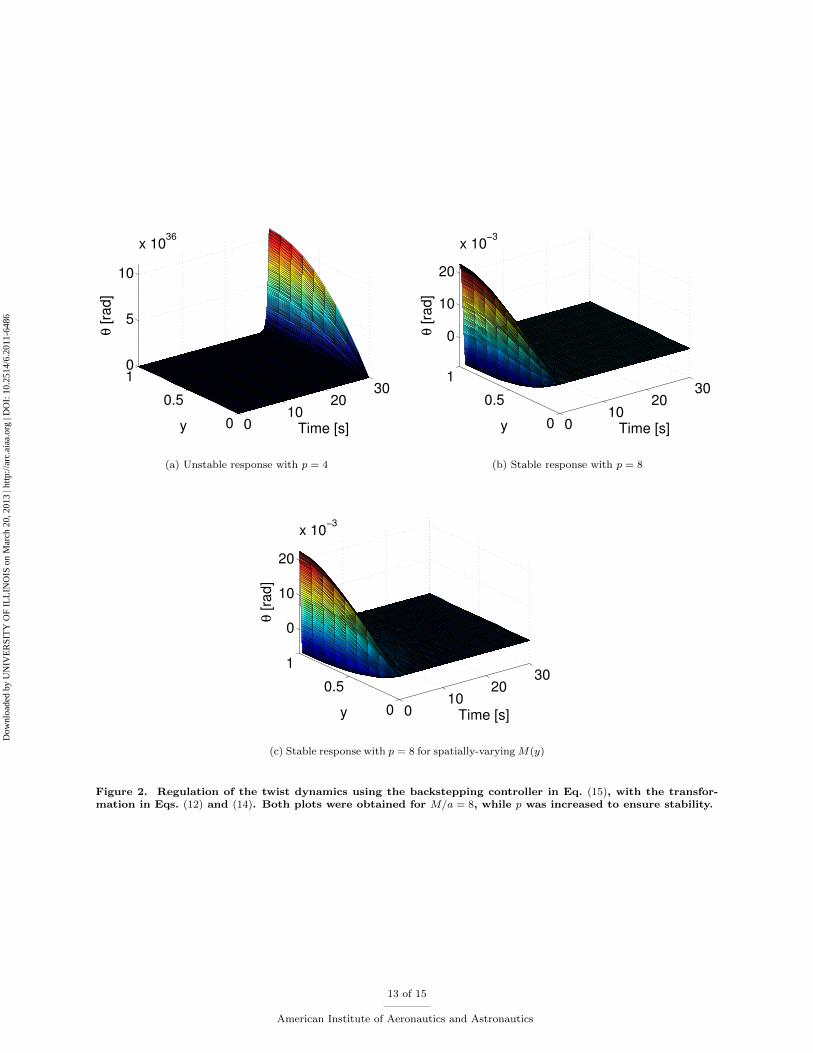
The reader will recall that is a scalar, and � = [�1 �2 : : : �n]T is a vector. The control s(t) is expressedsimilarly in terms of �, and � to obtain a set of ODEs which are simulated to approximate the responseof a twisting beam with boundary control. Figure 2 demonstrates the regulation of twist dynamics usingthe backstepping controller derived in Eq. (15), with the transformation in Eqs. (12) and (14). The valueof M=a was set to 8, where a = GJ=Ip. A value of p = 4 yielded an unstable response, while the responsewas stable for p = 8. Recall the following condition for stability with L = 1: p > M=a � �2=4 � 2:53. Thebackstepping controller works even when M(y) = M(1� y2) is used (to mimic an elliptical lift distributionover the wing) instead of a constant M(y) � M . The backstepping controller can be added on top of atracking controller.

Figure 3 shows the simulation of a wing actuated by tip control. The value of M=a was chosen so thatstability is assured without the need for a dedicated stabilizing controller. The �rst plot was obtained for acontroller designed assuming that all system parameters were known, whereas the right hand plot in the �rstrow was obtained for a system where the aerodynamics were assumed to be linear but unknown. The thirdplot (bottom row) was obtained for the case where the aerodynamics were assumed to be a�ne in �, with anunknown spatially varying coe�cient M(y). In all cases, the twist amplitude converges to the steady statevalue with satifactory transients. The error metric Eq. (4) is also seen to be very small.

12 of 15

American Institute of Aeronautics and Astronautics

Dow

nloa

ded

by U

NIV

ER

SIT

Y O

F IL

LIN

OIS

on

Mar

ch 2

0, 2

013

| http

://ar

c.ai

aa.o

rg |

DO

I: 1

0.25

14/6

.201

1-64

86

010

2030

0

0.5

10

5

10

x 1036

Time [s]y

θ [

rad

]

(a) Unstable response with p = 4

010

2030

0

0.5

1

0

10

20

x 10−3

Time [s]yθ [

rad

]

(b) Stable response with p = 8

010

2030

0

0.5

1

0

10

20

x 10−3

Time [s]y

θ [

rad

]

(c) Stable response with p = 8 for spatially-varying M(y)

Figure 2. Regulation of the twist dynamics using the backstepping controller in Eq. (15), with the transfor-mation in Eqs. (12) and (14). Both plots were obtained for M=a = 8, while p was increased to ensure stability.

13 of 15

American Institute of Aeronautics and Astronautics

Dow

nloa

ded

by U

NIV

ER

SIT

Y O

F IL

LIN

OIS

on

Mar

ch 2

0, 2

013

| http

://ar

c.ai

aa.o

rg |

DO

I: 1

0.25

14/6

.201

1-64

86

0

10

20

0

0.5

10

0.1

0.2

Time [s]y

θ [

rad

]

(a) All parameters known

0

10

20

0

0.5

10

0.1

0.2

Time [s]y

θ [

rad

]

(b) Aerodynamics unknown

0

10

20

0

0.5

10

0.1

0.2

Time [s]y

θ [

rad

]

(c) Spatially varying, unknown M(y)

-0.03

-0.02

-0.01

0

0.01

0.02

0 5 10 15 20 25 30

e

Time [s]

(d) Time history of e(t)

Figure 3. Twist pro�le of the wing as a function of time when the the adaptive controller in Eq. (24) is appliedat the wing tip. Three cases have been considered here. In the �rst case, the system dynamics are assumed tobe known. In the second case, the aerodynamics are assumed to be linear but unknown. In the third case, theaerodynamic moment is known to be of the form M(y)�, where M(y) is spatially varying and unknown. The

fourth plot shows the time history of e(t) =R 10 �dy �H, where H = 0:05.

14 of 15

American Institute of Aeronautics and Astronautics

Dow

nloa

ded

by U

NIV

ER

SIT

Y O

F IL

LIN

OIS

on

Mar

ch 2

0, 2

013

| http

://ar

c.ai

aa.o

rg |

DO

I: 1

0.25

14/6

.201

1-64

86

VII. Conclusions

This paper introduced a boundary control formulation for PDEs for the system output of a spatialintegral of the state. This output function closely resembles the spatial distribution of an aerodynamic force,i.e., lift, that can be properly shaped as a function of time to control the rigid motions of the aircraft. Inother words, the proposed boundary PDE control can signi�cantly simplify the control of exible aircraftby decoupling the force/torque control of the rigid body from the control of exible wings to output therequired force/torque input. In particular, the problem of beam twist was analysed in detail to illustratethe formulation. When the root twist angle was controlled, the output was seen to have an in�nite relativedegree with respect to the control input, and backstepping was employed for stabilization and tracking.Control laws based on this formulation ensure that the error between the reference output signal and theactual output decreases exponentially to zero when the system is fully known. When moment at the wing tipwas controlled, it was seen that the output had a relative degree of 2 with respect to the control input. Thisfacilitated the design of an adaptive controller along classical lines to ensure tracking. Both formulationswere demonstrated by simulations. Future work would focus on two fronts: (a) extending the proposedapproach to a wider class of nonlinearities, and (b) generalizing the method to the case of coupled bendingand twist.

Acknowledgment

This project was supported in part by the Air Force O�ce of Scienti�c Research (AFOSR) under theYoung Investigator Award Program (Grant No. FA95500910089) and the U.S. Army Research O�ce (ARO)under Award No W911NF-10-1-0296. The original problem of articulated wing aircraft was posed by Dr.Gregg Abate (AFRL).

References

1Paranjape, A. A., Chung, S.-J., Chakravarthy, A., and Hilton, H. H., \Dynamics and Performance of a Tailless MAVwith Flexible Articulated Wings," AIAA Journal, in review.

2Paranjape, A. A., Chung, S.-J., and Selig, M. S., \Flight Mechanics of a Tailless Articulated Wing Aircraft," Bioinspi-ration & Biomimetics, Vol. 6, No. 2, 2011.

3Tran, D. T., and Lind, R., \Parameterizing Stability Derivatives and Flight Dynamics with Wing Deformation," AIAAAtmospheric Flight Mechanics Conference 2010, AIAA Paper 2010-8227.

4Ifju, P.G., Jenkins, D. A., Ettinger, S., Yongsheng L., Shyy, W., and Waszak, M. R., \Flexible-wing-based micro airvehicles," AIAA 2002 - 0705.

5Shyy, W., et al., \Recent Progress in Flapping Wing Aerodynamics and Aeroelasticity," Progress in Aerospace Sciences,Vol. 46, No. 7, 2010, pp.284-327.

6Abdulrahim, M., Garcia, H., and Lind, R., \Flight Characteristics of Shaping the Membrane Wing of a Micro AirVehicle," Journal of Aircraft, Vol. 42, No. 1, 2005, pp.131 - 137.

7Russell D. L., \Controllability and Stabilizability Theory for Linear Partial Di�erential Equations: Recent Progress andOpen Questions," Siam Review, Vol. 20, No. 4, 1978, pp. 639 739.

8Krstic M., and Smyshlyaev A., \Adaptive Control of PDEs," Ann. Rev. in Control, Vol. 32, No. 2, 2008, pp. 149 - 160.9Krstic, M., and Smyshlyaev, A., Boundary Control of PDEs: A Course on Backstepping Designs, Ch. 7, pp. 79-88,

Advances in Design and Control, SIAM, 2008.10Christo�des, P. D., and Daoutidis, P., \Feedback control of hyperbolic PDE systems," AIChE Journal, Vol. 42, No. 11,

1996, pp. 3063 - 3086.11Christo�des P. D., and Daoutidis, P., \Finite-Dimensional Control of Parabolic PDE Systems Using Approximate Inertial

Manifolds," Proceedings of the 36th IEEE Conference on Decision and Control, 1997, pp. 1068 - 1073.12Lohmiller, W., and Slotine, J.-J. E., \Contraction Analysis of Nonlinear Distributed Systems," International Journal of

Control, Vol. 78, No. 9, 2005, pp. 678-688.13Hodges, D. H., and Pierce, G. A., Introduction to Structural Dynamics and Aeroelasticity, Cambridge Aerospace Series

(No. 15), Cambridge University Press, 2002, Ch. 2, pp. 59 - 66.14De Queiroz, M., Dawson, D. M., Agarwal, M., and Zhang, F., \Adaptive Nonlinear Boundary Control of a Flexible Link

Robotic Arm," IEEE Trans. Robotics and Automation, Vol. 15, No. 4, 1999, pp. 779 - 787.15He, W., Ge, S. S., How, B. V. E., Choo, Y. S., and Hong, K.-S., \Robust Adaptive Boundary Control of a Flexible

Marine Riser with Vessel Dynamics," Automatica, Vol. 47, 2011, pp. 722 - 732.16Bieniawski, S., and Kroo, I. M., \Flutter Suppression Using Micro-Trailing Edge E�ectors," 44th

AIAA/ASME/ASCE/AHS Structures, Structural Dynamics, and Materials Conference, AIAA 2003 - 1941.17Chung, S.-J., and Dorothy, M., \Neurobiologically Inspired Control of Engineered Flapping Flight," Journal of Guidance,

Control and Dynamics, Vol. 33, No. 2, 2010, pp. 440 - 453.18McCormick, B. W., Aerodynamics, Aeronautics and Flight Mechanics, Wiley, 2nd Ed., 1994.19Khalil, H. K., Nonlinear Systems, 3rd Ed., Pearson Education, Upper Saddle, NJ, 2000, pp. 340-345.

15 of 15

American Institute of Aeronautics and Astronautics

Dow

nloa

ded

by U

NIV

ER

SIT

Y O

F IL

LIN

OIS

on

Mar

ch 2

0, 2

013

| http

://ar

c.ai

aa.o

rg |

DO

I: 1

0.25

14/6

.201

1-64

86