Approximation of stationary statistical properties of

dissipative dynamical systems: time discretization

Xiaoming Wang∗

Department of Mathematics, Florida State University, Tallahassee, FL32306

September 11, 2008

Abstract

We consider temporal approximation of stationary statistical properties of dissipa-tive complex dynamical systems. We demonstrate that stationary statistical propertiesof the time discrete approximations (numerical scheme) converge to those of the un-derlying continuous dissipative complex dynamical system under three very naturalassumptions as the time step approaches zero. The three conditions that are sufficientfor the convergence of the stationary statistical properties are: (1) uniform dissipativityof the scheme (in the sense of pre-compactness of the union of the global attractors forthe numerical approximations); (2) uniform (with respect to initial data from the unionof the global attractors) convergence of the solutions of the numerical scheme to thesolution of the continuous system on the unit time interval [0, 1]; and (3) the uniform(with respect to initial data from the union of the global attractors) continuity of thesolutions to the continuous dynamical system on the unit time interval [0, 1]. The con-vergence of the global attractors is established under weaker assumptions. Applicationto the infinite Prandtl number model for convection is discussed.

keywords: stationary statistical property, invariant measure, global attractor, dissipa-tive system, time discretization, uniformly dissipative scheme, infinite Prandtl number modelfor convection, Nusselt number

1 Introduction

Many dissipative dynamical systems arising in physical applications possess very complex be-havior with abundant instability and sensitive dependence on initial data and parameters[29].It is well-known that statistical properties of these kind of systems are much more important,physically relevant and stable than single trajectories [11, 18, 20, 22, 23, 32].

∗wxm@math.fsu.edu, 65P99, 37M25, 65M12, 37L40, 76F35, 76F20, 37L30, 37N10, 35Q35,

1

For a given abstract autonomous continuous in time dynamical system determined by asemi-group S(t), t ≥ 0 on a separable Banach space H , we recall that if the system reachesa statistical equilibrium in the sense that the statistics are time independent (stationary sta-tistical properties), the probability measure µ on H that describes the stationary uncertainty(stationary statistical properties) can be characterized via either the strong (pull-back) orweak (push-forward) formulation [11, 20, 22, 32, 33].

Definition 1 (Invariant Measure (Stationary Statistical Solution)). Let S(t), t ≥ 0 be acontinuous semi-group on a Banach space H which generates a dynamical system on H. ABorel probability measure µ on H is called an Invariant Measure(Stationary StatisticalSolution) of the dynamical system if

µ(E) = µ(S−1(t)(E)), ∀t ≥ 0, ∀E ∈ B(H) (1)

where B(H) represents the σ-algebra of all Borel sets on H. Equivalently, the invariant mea-sure µ can be characterized through the following push-forward weak invariance formulation

∫

H

Φ(u) dµ(u) =

∫

H

Φ(S(t)u) dµ(u), ∀t ≥ 0 (2)

for all bounded continuous test functionals Φ.Invariant measure (stationary statistical solution) for a discrete dynamical system gen-

erated by a map Sdiscrete on a Banach space H is defined in a similar fashion with thecontinuous time t replaced by discrete time n = 0, 1, 2, · · ·.

Another popular object utilized below associated with long time behavior of a dynamicalsystem is the global attractor which we recall for convenience [11, 13, 29].

Definition 2 (Global Attractor and Dissipative System). Let S(t), t ≥ 0 be a continuoussemi-group on a Banach space H which generates a continuous dynamical system on H.A set A ⊂ H is called the global attractor of the dynamical system if the following threeconditions are satisfied.

1. A is compact in H.

2. A is invariant under the flow, i.e.

S(t)A = A, for all t ≥ 0. (3)

3. A attracts all bounded sets in H, i.e., for every bounded set B in H,

limt→∞

distH(S(t)B,A) = 0. (4)

2

Here, distH denotes the Hausdorff semi-distance in H between two subsets which is definedas

distH(A,B) = supa∈A

infb∈B

‖a− b‖H (5)

where ‖ · ‖H = ‖ · ‖ denotes the norm on H.The global attractor for a discrete dynamical system induced by a map Sdiscrete on a

Banach space H is defined in a similar fashion with the continuous time t replaced by discretetime n = 0, 1, 2, · · ·.

A dynamical system is called dissipative if it possesses a global attractor.

It is easy to see, thanks to the invariance and the attracting property, that the globalattractor, when it exists, is unique [13, 29]. We also caution the reader that our definitionof dissipativity may be slightly different from the traditional notation [13, 29].

We are usually interested in∫

HΦ(u) dµ(u) (statistical average) for various test functionals

Φ (observable). Since we normally do not know the invariant measure µ a priori, one of thecommonly used methods in calculating the statistical quantity is to substitute spatial averageby long time average under Boltzmann’s assumption of ergodicity ([11, 20, 22, 33])

∫

H

Φ(u) dµ(u) = limt→∞

1

t

∫ t

0

Φ(S(s)u) ds.

Although this formulation may not make sense all the time since the long time averagemay not exist, one can always replace the long time limit by Banach (generalized) limitwhich are bounded linear functionals on the space of bounded functions that agrees with theusual long time limit on those functions whenever the long time limit exists [21]. One mayshow via the so-called Bogliubov-Krylov argument that these generalized long time averageover trajectory leads to invariant measure (may depend on the chosen Banach limit andinitial datum u) of the system for appropriate dissipative dynamical systems such as the twodimensional incompressible Navier-Stokes system and the infinite Prandtl number model forconvection system discussed below [11, 32, 36].

Due to the presumed complexity of the dynamics, it is foreseeable that physically inter-esting stationary statistical properties need to be calculated using numerical methods. Evenunder the ergodicity assumption, it is not at all clear that classical numerical schemes whichprovide accurate approximation on finite time interval will remain meaningful for stationarystatistical properties (long time properties) since small error will be amplified and accumu-lated over long time except in the case that the underlying dynamics is asymptotically stable[12, 14, 19] where statistical approach is not necessary since there is no chaos. Therefore, itis of great importance and a challenge to search for numerical methods that are able to cap-ture stationary statistical properties of infinite dimensional complex dynamical system. Wewill focus on dissipative system and time discretization here since long time approximationseems to be the key issue involved.

As we shall demonstrate below that if the system and the scheme possess three verynatural properties (1) uniform dissipativity in the sense that the scheme possesses global

3

attractor for small enough time step and the union of these global attractors (for differenttime steps) is pre-compact in the phase space; (2) uniform convergence of the numericalscheme for data from the support of the invariant measures on the unit time interval [0, 1]modulo initial layer; and (3) the continuous dynamical system is uniformly continuous (fordata from the support of the invariant measures) on the unit time interval [0, 1], then thestationary statistical properties of the scheme will converge to stationary statistical propertiesof the continuous dynamical system. Our result will be presented in an abstract fashion inorder to clarify the central issues and to provide well-organized means for discussing theproblems. We also hope that our work will stimulate further work on accurate and efficientnumerical schemes for stationary statistical properties of infinite dimensional dissipativesystems.

It is easy to see that the assumptions are natural. Since the underlying dynamical systemis dissipative, it is natural to require that the numerical scheme inherit the dissipativityof the continuous in time system so that the scheme is uniformly dissipative (for smalltime steps). The uniform convergence of the numerical scheme for initial data from theglobal attractor on the unit time interval is also expected from most reasonable numericalschemes. The strong continuity of the underlying dynamical system on the unit time intervaluniform with respect to initial data from the union of the global attractors is natural formost continuous dissipative dynamical systems. Once the desired natural conditions arediscovered, the proof of the main result is relatively straightforward although verifying thesethree sufficient conditions for each application may be highly non-trivial (see section 3 for arelatively easy application to the infinite Prandtl number model for convection with a linearsemi-implicit scheme).

Although we are not aware of any work on the convergence of stationary statisticalproperties of numerical schemes for chaotic PDEs except our previous work [3, 4] (see [5] forthe case of map on the unit interval), there have been a lot of work on temporal approximationof dissipative dynamical systems such as the two dimensional incompressible Navier-Stokessystem and the one-dimensional Kuramoto-Sivashinsky equation (see [12, 15, 17, 25, 26,30, 9, 10] among others). These authors were mostly interested in the long time stabilityof the scheme in the sense of deriving uniform in time bounds on the scheme (sometimesbound in the phase space H only which is not sufficient for uniform dissipativity although itmay be sufficient for the convergence of the global attractors), and none of them discussedstatistical properties. Our result on the convergence of stationary statistical properties maybe viewed as an abstraction and generalization of [3, 4]. See [8] for the heat bath approachto computing invariant measure for finite dimensional systems.

A by-product of the convergence analysis of the invariant measures presented here isthe convergence of the global attractors of the scheme to that of the underlying system.This is also within expectation since the global attractors carry the support of the invari-ant measures. The convergence of the global attractors under time discretization has beendiscussed for the two dimensional Navier-Stokes system, reaction-diffusion equation, andfor finite-dimensional dynamical systems [25, 27, 15] among others. Therefore our resulton the convergence of global attractors may be viewed as a generalization and abstraction

4

of these results. However, we would like to point out that the convergence of the globalattractors can be established under much weaker assumption. One only needs the uniformboundedness of the union of the global attractors K, instead of the pre-compactness (plusfinite time uniform convergence for data from K). Because of this important distinction, itis possible to have schemes that are able to capture the global attractor asymptotically butnot necessarily the stationary statistical properties (invariant measures). There are also in-teresting works on persistence under approximation of various invariant sets (such as steadystate, time periodic orbit, inertial manifold etc) both for PDEs and ODEs under appropriateassumptions (such as spectral gap condition that is usually associated with inertial manifoldtheory, see [27, 16, 28, 29] and the references therein). We would also like to point out thatthe convergence of invariant sets and the convergence of stationary statistical properties aretwo related but very different issues associated with the long time behavior. It is easy toconstruct two dynamical systems with exactly the same global attractor or inertial manifoldbut with totally different dynamics or stationary statistical properties.

The rest of the manuscript is organized as follows: in section 2 we prove the main results,namely the convergence of stationary statistical properties and the global attractors underthe three natural hypotheses; in section 3 we discuss an application of the main results tothe infinite Prandtl number model for convection. The choice of application is both for itsphysical significance and mathematical simplicity so that an essentially self-contained shortexposition is possible and we believe that our main abstract theorem applies to many otherdissipative systems and schemes. We then provide conclusion and remarks in the fourth/lastsection.

2 Main results: abstract formulation

Here we show our main results, namely, uniform dissipativity plus finite time uniform conver-gence of the time discrete approximation together with the finite time uniform continuity ofthe underlying dynamical system imply convergence of the stationary statistical properties/ invariant measures.

Throughout this section, all semigroups are assumed to be continuous in the sense thatS(t), t ≥ 0 and Sk are continuous operators on H .

Theorem 1 (Convergence of Stationary Statistical Properties). Let S(t), t ≥ 0 be a con-tinuous semi-group on a separable Hilbert space H which generates a continuous dissipativedynamical system (in the sense of possessing a compact global attractor A) on H. LetSk, 0 < k ≤ k0 be a family of continuous maps on H which generates a family of discretedissipative dynamical system (with global attractor Ak) on H. Suppose that the followingthree conditions are satisfied.

H1: [ Uniform dissipativity] There exists a k1 ∈ (0, k0) such that Sk, 0 < k ≤ k1 isuniformly dissipative in the sense that

K =⋃

0<k≤k1

Ak (6)

5

is pre-compact in H.

H2: [ Uniform convergence on the unit time interval] Sk uniformly converges to S on theunit time interval (modulo an initial layer) and uniformly for initial data from theglobal attractor of Sk in the sense that for any t0 ∈ (0, 1)

limk→0

supu∈Ak ,nk∈[t0,1]

‖Snk u− S(nk)u‖ = 0. (7)

H3: [ Uniform continuity of the continuous system] S(t), t ≥ 0 is uniformly continuouson K on the unit time interval in the sense that for any T ∗ ∈ [0, 1]

limt→T ∗

supu∈K

‖S(t)u− S(T ∗)u‖ = 0. (8)

Then the invariant measures of the discrete dynamical system Sk, 0 < k ≤ k0 converge toinvariant measures of the continuous dynamical system S. More precisely, let µk ∈ IMk

where IMk denotes the set of all invariant measures of Sk. There must exist a subsequence,still denoted µk, and µ ∈ IM (an invariant measure of S(t)), such that µk weakly con-verges to µ, i.e.,

µk µ, as k → 0. (9)

Moreover, extremal statistics converge in upper-semi-continuous fashion in the sense thatfor any bounded continuous functional Φ on the phase space H, there exist ergodic invariantmeasures µk ∈ IMk and an ergodic invariant measure µ ∈ IM, such that

supu0∈H

lim supN→∞

1

N

N∑

n=1

Φ(Snk (u0)) =

∫

H

Φ(u) dµk(u), ∀k, (10)

supu0∈H

lim supT ∗→∞

1

T ∗

∫ T ∗

0

Φ(S(t)u0) dt =

∫

H

Φ(u) dµ(u), (11)

lim supk→0

supu0∈H

lim supN→∞

1

N

N∑

n=1

Φ(Snk (u0)) ≤ sup

u0∈H

lim supT ∗→∞

1

T ∗

∫ T ∗

0

Φ(S(t)u0) dt. (12)

Proof: Since K =⋃

0<k≤k1Ak is pre-compact in H and since all invariant measures are

supported on the global attractor [11, 36] and µk ∈ IMk, we see that µk is tight in thespace of all Borel probability measures on H thanks to Prokhorov’s theorem [1, 21, 11].Hence it must contain a weakly convergent subsequence (still denoted µk) which weaklyconverges to a Borel probability measure µ on H , i.e.

∫

H

ϕ(u) dµk(u) →∫

H

ϕ(u) dµ(u), as k → 0.

Our goal is to show that µ is invariant under S(t).

6

Now we fix a T ∗ ∈ (0, 1] and let nk = ⌊T ∗

k⌋ be the floor of T ∗

k(the largest integer

dominated by T ∗

k), and let ϕ be any smooth (C1) test functional (observable) with compact

support.Since µk ∈ IMk, we have by the weak invariance of µk under Sk and weak convergence

∫

H

ϕ(Snk

k u) dµk(u) =

∫

H

ϕ(u) dµk(u) →∫

H

ϕ(u) dµ(u), as k → 0.

On the other hand,∫

H

ϕ(Snk

k u) dµk(u)

=

∫

H

ϕ(S(T ∗)u) dµk(u) +

∫

H

(ϕ(S(nkk)u) − ϕ(S(T ∗)u)) dµk(u) +

∫

H

(ϕ(Snk

k u) − ϕ(S(nkk)u)) dµk(u)

For the first term, since S(t) is continuous, ϕ(S(T ∗)u) is bounded and continuous in u.Hence we have

∫

H

ϕ(S(T ∗)u) dµk(u) →∫

H

ϕ(S(T ∗)u) dµ(u), as k → 0.

We also have, thanks to the uniform convergence assumption, the mean value theorem, theuniform boundedness of the derivative of the smooth (C1) test functional (observable) withcompact support, for u ∈ Ak,

|ϕ(Snk

k u) − ϕ(S(nkk)u)| ≤ supu∈H

‖ϕ′(u)‖ supu∈Ak

‖Snk

k u− S(nkk)u‖

≤ supu∈H

‖ϕ′(u)‖ supu∈Ak ,nk∈[ T∗

2,T ∗]

‖Snk u− S(nk)u‖

→ 0, as k → 0,

1 and hence, since the support of invariant measure µk is included in the global attractorAk, [11, 36]

∫

H

(ϕ(Snk

k u) − ϕ(S(nkk)u)) dµk(u) → 0, as k → 0.

Moreover,

|ϕ(S(nkk)u) − ϕ(S(T ∗)u)| ≤ supu∈H

‖ϕ′(u)‖ supu∈Ak

‖S(nkk)u − S(T ∗)u‖ → 0, as k → 0

by the uniform continuity of S(t) at t = T ∗ and u ∈ K since nkk = ⌊T ∗

k⌋k → T ∗ as k → 0.

This further implies,∫

H

(ϕ(S(nkk)u) − ϕ(S(T ∗)u)) dµk(u) → 0, as k → 0.

1We only need limk→0 supu∈Ak

supT∗− 1

k≤nk≤T∗ ‖Sn

ku − S(nk)u‖ = 0, ∀T ∗ ∈ (0, 1].

7

Combining the estimates above, we have

∫

H

ϕ(Snk

k u) dµk(u) →∫

H

ϕ(S(T ∗)u) dµ(u), as k → 0.

Therefore∫

H

ϕ(S(T ∗)u) dµ(u) =

∫

H

ϕ(u) dµ(u)

which is exactly the weak invariance (2) for the smooth (C1) test functional (observable)with compact support and T ∗ ∈ (0, 1].

For a general bounded continuous test functional ϕ, we can first approximate it by finitedimensional test functional of the form ϕPm where Pm is the orthogonal projection onto them-dimensional subspace spanned by the first m elements of a given (fixed) orthonormal basisof H (this is where we need H to be a separable Hilbert space). We can then approximateϕPm by smooth test functionals with compact support using mollifiers and truncation sinceonly the value of ϕPm on the compact global attractor is relevant for statistics. This provesshort time weak invariance (2) for any bounded continuous test functional φ and T ∗ ∈ (0, 1].

Now for a general T ∗∗ > 1, we exists a unique positive integer n and T∗ ∈ (0, 1] such thatT ∗∗ = n+ T∗. Hence

∫

H

ϕ(S(T ∗∗)u) dµ(u) =

∫

H

ϕ(Sn(1)S(T∗)u) dµ(u)

=

∫

H

ϕ(S(T∗)u) dµ(u)

=

∫

H

ϕ(u) dµ(u)

where we have utilized the semi-group property of S(t), the strong continuity of S(t) andthe short time weak invariance that we proved above with T ∗ = 1 n times and T ∗ = T∗ onetime.

This ends the proof of the convergence of the invariant measures.As for the extremal statistics, it is easy to see that due to the uniform dissipativity, for any

given bounded continuous test functional Φ, there exist ergodic invariant measures µk andµ such that the extreme of temporal averages are equivalent to spatial averages with respectto these ergodic invariant measures [36, 11, 33], as stated in (10, 11). This is a manifestationof the fact that the extremal points of the set of invariant measures must be ergodic. Asfor the upper semi-convergence of the extremal statistics stated in (12), we have, thanks tothe uniform dissipativity and Prokhorov’s theorem, there exists a subsequence (still denotedµk) and ν ∈ IM such that

µk → ν, as k → 0,

lim supk→0

supu0∈H

lim supN→∞

1

N

N∑

n=1

Φ(Snk (u0)) = lim sup

k→0

∫

H

Φ(u) dµk.

8

Since IM is compact in the space of Borel probability measures on H , there exists anergodic invariant measure νmax ∈ IM such that supµ∈IM

∫

HΦ(u) dµ =

∫

HΦ(u) dνmax [36].

Therefore

lim supk→0

supu0∈H

lim supN→∞

1

N

N∑

n=1

Φ(Snk (u0)) = lim sup

k→0

∫

H

Φ(u) dµk

=

∫

H

Φ(u) dν

≤ supµ∈IM

∫

H

Φ(u) dµ

=

∫

H

Φ(u) dνmax

= limT ∗→∞

1

T ∗

∫ T ∗

0

Φ(S(t)u0) dt

≤ supu0∈H

lim supT ∗→∞

1

T ∗

∫ T ∗

0

Φ(S(t)u0) dt.

This completes the proof of the theorem.

Next, we show the convergence of the global attractors under weaker assumptions, namelythe uniform boundedness of K (the union of the global attractors), and uniform convergenceon finite time interval (modulo an arbitrary initial layer).

Proposition 1 (Convergence of Global Attractors). Let S(t), t ≥ 0 be a continuous semi-group on a Banach space H which generates a dissipative dynamical system (in the senseof possessing a compact global attractor A) on H. Let Sk, 0 < k ≤ k0 be a family ofcontinuous maps on H which generates a family of discrete dissipative dynamical system(with global attractor Ak) on H. Suppose that the following two conditions are satisfied.

H4: [ Uniform boundedness] There exists a k1 ∈ (0, k0] such that Sk, 0 < k ≤ k1 isuniformly bounded in the sense that

K =⋃

0<k≤k1

Ak (13)

is bounded in H.

H5: [ Finite time uniform convergence] Sk uniformly converges to S on any finite time in-terval (modulo any initial layer) and uniformly for initial data from the global attractorof the scheme in the sense that there exists t0 > 0 such that for any T ∗ > t0 > 0

limk→0

supu∈Ak ,nk∈[t0,T ∗]

‖Snk u− S(nk)u‖ = 0. (14)

9

Then the global attractors converge in the sense of Hausdorff semi-distance, i.e.

limk→0

distH(Ak,A) = 0. (15)

Proof: Since K is bounded, for any given ǫ > 0, there exists a Tǫ > t0 > 0 such that

distH(S(t)K,A) <ǫ

2, ∀t ≥ Tǫ

because the global attractor A attracts all bounded set, in particular K.Now let uk ∈ Ak. Since the global attractor Ak is invariant under Sk, there exists a

vk ∈ Ak such that uk = Snk

k vk where nk = ⌊Tǫ+1k

⌋.Thanks to the uniform convergence on [Tǫ, Tǫ+1] and u ∈ K, we have, there exists kǫ > 0

such that‖uk − S(nkk)vk‖ = ‖Snk

k vk − S(nkk)vk‖ <ǫ

2, k ≤ kǫ.

This implies that

distH(Ak,A) = supuk∈Ak

dist(uk,A)

≤ supuk∈Ak

(‖uk − S(nkk)vk‖ + dist(S(nkk)vk,A))

≤ ǫ, k ≤ kǫ.

This completes the proof for the convergence of the global attractors.

We would like to reiterate the point that the uniform boundedness assumption H4 ismuch weaker that the uniform dissipativity assumption H1 for infinite dimensional systemsalthough they are equivalent for finite dimensional systems. This is an important differenceand hence it is theoretically possible to have schemes that are able to capture the globalattractor asymptotically but not the invariant measures necessarily. Conditions H5 and H2are roughly equivalent in some sense. They are usually valid for reasonable numerical schemes(see below for an example on the infinite Prandtl number model). Therefore convergenceof the global attractors is usually easier to establish than the convergence of the invariantmeasures (stationary statistical properties).

In application, the discrete dynamical systems Sk are usually generated by one timestep discretization (numerical scheme) with time step k. In another word, un+1 = Sk(u

n)is the solution to the numerical scheme. The uniform dissipativity of the numerical schemeis customary established via the existence of a uniform (in time step) absorbing ball inanother separable Hilbert space V which is compactly imbedded in H in the case of stronglydissipative system (see the next section for an example). However, this may not be feasiblefor weakly dissipative systems such as the Darcy-Boussinesq system for convection in fluidsaturated porous media, or weakly damped driven Schrodinger equation. The finite timeuniform convergence comes with classical numerical analysis for reasonable schemes (seenext section for an example). The uniform continuity of the underlying continuous dynamicalsystem is also easily verified for reasonable systems.

10

3 Application to the infinite Prandtl number model for

convection

Here we illustrate an application of the main result to the following infinite Prandtl numberfor convection [2, 31, 6, 34, 7]

∇p = ∆u +RakT, ∇ · u = 0, u|z=0,1 = 0, (16)

∂T

∂t+ u · ∇T = ∆T, T |z=0 = 1, T |z=1 = 0 (17)

where u is the Eulerian velocity of the fluid, p represents the kinematic pressure of the fluid,T is the temperature of the fluid, k is a unit vector in the z direction, Ra is the Rayleighnumber measuring the ratio of differential heating over overall dissipation, and we assumethat the fluids occupy the (non-dimensionalized) region Ω = [0, Lx] × [0, Ly] × [0, 1] withperiodicity imposed in the horizontal directions for simplicity.

The choice of this example is both for its physical significance and for its mathematicalsimplicity so that we may have an essentially self-contained short exposition. It is well-knownthat this system possesses turbulent behavior at large Rayleigh number [2, 6, 18, 31]. Theconvergence of the stationary statistical properties for another class of semi-implicit schemeswas discussed in [3, 4] utilizing Liouville type equation approach. The scheme that we studyhere has an added advantage over the schemes that we investigated earlier in the sense thatthe discretization is independent of any ad-hoc background temperature profile τ (to beintroduced in (22)).

One of the most important statistical quantities in convection is the Nusselt number[2, 6, 7, 18, 35] quantifying the heat transport in the vertical direction which is the statisticscorresponding to the functional

Φ(θ) = Ra

∫

Ω

A−1(kθ)3θ dx =

∫

Ω

u3θ dx

where A denotes the Stokes operator with the associated boundary conditions and viscosityone, and A−1(kθ)3 represents the third component (vertical velocity) of A−1(kθ). In anotherword, u = A−1f solves the following Stokes system

−∆u + ∇p = f , ∇ · u = 0,

u|z=0,1 = 0, u periodic in x, y.

Although this Φ is not bounded, for any pre-compact set K (in particular the union of theglobal attractors of the scheme), we can easily replace it by a bounded continuous functionalΦ which agrees with Φ on K and hence the statistical averages of Φ and Φ are the samesince the support of all interested invariant measures is included in K. The replacement ispossible due to the pre-compactness of K (presumed, to be verified below). Our result onthe convergence of the Nusselt number, i.e. (12) with the Φ given above, complements thewell-known variational approach [6] since our result indicates that the numerics will providean asymptotic lower bound for the maximal Nusselt number while the variational approachprovides a rigorous upper bound.

11

3.1 A semi-implicit scheme

Notice that the infinite Prandtl number model can be written as a non-local non-linearadvection diffusion equation for the temperature field

∂T

∂t+Ra A−1(kT ) · ∇T = ∆T, T |z=0 = 1, T |z=1 = 0 (18)

where A denotes the Stokes operator with the associated boundary conditions and viscosityone.

We then propose the following semi-implicit scheme for the infinite Prandtl number model

T n+1k − T n

k

k+RaA−1(kT n

k ) · ∇T n+1k = ∆T n+1

k (19)

where T nk denotes the approximate solution at time kn with k being the time step.

Our goal now is to show that the stationary statistical properties of this scheme convergeto those of the infinite Prandtl number model as the time step k approaches zero.

In order to accomplish this goal utilizing our main result proved in the previous section,we rewrite the scheme in the perturbative variable θ as usual so that the phase space is theHilbert space H = L2(Ω)

θn+1k − θn

k

k+RaA−1(kθn

k ) · ∇θn+1k +RaA−1(kθn

k )3τ′(z) = ∆θn+1

k + τ ′′(z) (20)

where θnk = T n

k − τ with τ(z) being an add-hoc background temperature profile (to bespecified below) which satisfies the non-homogeneous Dirichlet boundary condition of T n

k ,and we are searching for solution in the spaceH1

0,per (the subspace ofH1 with zero trace/valueat z = 0, 1 and periodic in the horizontal directions). Here A−1(kθ)3 represents the thirdcomponent (vertical velocity) of A−1(kθ).

The infinite Prandtl number model (18) can be written in the perturbative variable θ aswell

∂θ

∂t+RaA−1(kθ) · ∇θ +RaA−1(kθ)3τ

′(z) = ∆θ + τ ′′(z). (21)

Following [6], we set the background temperature profile τ to be a locally smoothed(mollified) version of the following piecewise linear function

τ(z) =

1 − zδ, 0 ≤ z ≤ δ,

0, δ ≤ z ≤ 1.(22)

The choice of the parameter δ will be specified later in (26).We remark that the scheme (20) is different from the scheme that we investigated earlier

[3, 4] where the schemeθn+1

k−θn

k

k+RaA−1(kθn

k )·∇θn+1k +RaA−1(kθn+1

k )3τ′(z) = ∆θn+1

k +τ ′′(z)was studied. The new scheme (20) has the advantage that it is independent of the ad-hoc

12

background profile τ since it can be written in terms of the temperature field T only as isclear in (19).

It is easy to see that the well-posedness of the scheme (20) follows from the weak formu-lation∫

Ω

(1

kθn+1

k +RaA−1(kθnk )·∇θn+1

k )ψ+

∫

Ω

∇θn+1k ·∇ψ =

∫

Ω

(1

kθn

k+τ ′′−RaA−1(kθnk )3τ

′(z))ψ, ∀ψ ∈ H10,per,

(23)the identity

∫

ΩA−1(kθn

k ) · ∇θn+1k θn+1

k = 0, ∀θn+1k ∈ H1

0,per, θnk ∈ L2, and the Lax-Milgram

theorem [21]. Therefore, we have a discrete dynamical system Sk defined on the Hilbertspace

H = L2(Ω) (24)

given bySk(θ

nk ) = θn+1

k . (25)

We notice that Sk in fact maps H into H10,per which is a direct consequence of the weak

formulation.In order to apply the main result proved in the previous theorem to the current situation,

we will verify the three conditions postulated in the main theorem. These will be the goalof the next three subsections.

3.2 Uniform dissipativity

Here we demonstrate the uniform dissipativity, i.e., H1, of the scheme (20) with appropriatechoice of δ.

Here and below, the cjs denote generic constants independent of k, n and the initialdata unless otherwise stated (but which may depend on the Rayleigh number). Here and

elsewhere ‖θ‖ =√

∫

Ω|θ|2 denotes the spatial L2 norm of θ, and ‖θ‖∞ = esssupΩ|θ| denotes

the spatial L∞ norm of θ.We first derive a uniform bound in the L2 space. For this purpose we take the inner

product of the scheme (20) with ψ = θn+1k and utilize the identity (a− b, a) = 1

2(|a|2 − |b|2 +

|a− b|2), and we have

1

2k(‖θn+1

k ‖2 − ‖θnk‖2 + ‖θn+1

k − θnk‖2) + ‖∇θn+1

k ‖2

≤ ‖τ ′‖‖∇θn+1k ‖ +Ra|

∫

Ω

τ ′(z)(A−1(kθnk ))3θ

n+1k |

≤ ‖τ ′‖2 +1

4‖∇θn+1

k ‖2 +Ra|∫

Ω

τ ′(z)(A−1(kθnk ))3θ

n+1k |

where we have used the identity∫

ΩA−1(kθn

k ) · ∇θn+1k θn+1

k = 0 one more time.

13

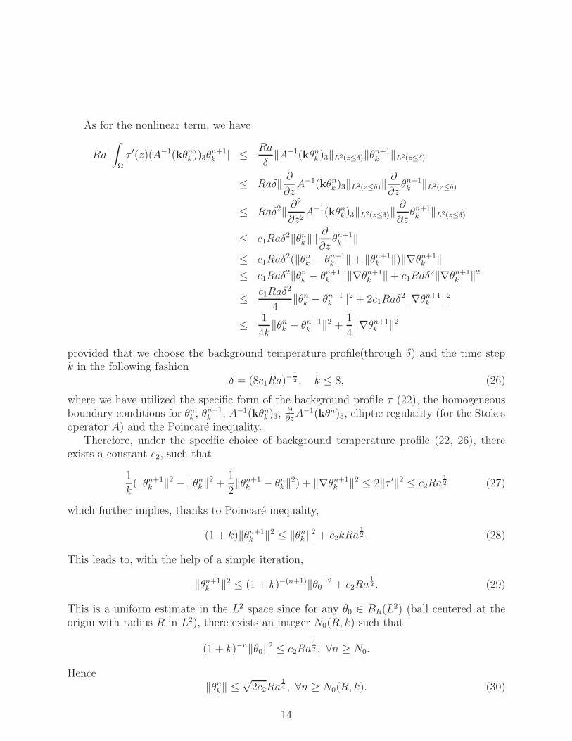
As for the nonlinear term, we have

Ra|∫

Ω

τ ′(z)(A−1(kθnk ))3θ

n+1k | ≤ Ra

δ‖A−1(kθn

k )3‖L2(z≤δ)‖θn+1k ‖L2(z≤δ)

≤ Raδ‖ ∂∂zA−1(kθn

k )3‖L2(z≤δ)‖∂

∂zθn+1

k ‖L2(z≤δ)

≤ Raδ2‖ ∂2

∂z2A−1(kθn

k )3‖L2(z≤δ)‖∂

∂zθn+1

k ‖L2(z≤δ)

≤ c1Raδ2‖θn

k‖‖∂

∂zθn+1

k ‖≤ c1Raδ

2(‖θnk − θn+1

k ‖ + ‖θn+1k ‖)‖∇θn+1

k ‖≤ c1Raδ

2‖θnk − θn+1

k ‖‖∇θn+1k ‖ + c1Raδ

2‖∇θn+1k ‖2

≤ c1Raδ2

4‖θn

k − θn+1k ‖2 + 2c1Raδ

2‖∇θn+1k ‖2

≤ 1

4k‖θn

k − θn+1k ‖2 +

1

4‖∇θn+1

k ‖2

provided that we choose the background temperature profile(through δ) and the time stepk in the following fashion

δ = (8c1Ra)− 1

2 , k ≤ 8, (26)

where we have utilized the specific form of the background profile τ (22), the homogeneousboundary conditions for θn

k , θn+1k , A−1(kθn

k )3,∂∂zA−1(kθn)3, elliptic regularity (for the Stokes

operator A) and the Poincare inequality.Therefore, under the specific choice of background temperature profile (22, 26), there

exists a constant c2, such that

1

k(‖θn+1

k ‖2 − ‖θnk‖2 +

1

2‖θn+1

k − θnk‖2) + ‖∇θn+1

k ‖2 ≤ 2‖τ ′‖2 ≤ c2Ra1

2 (27)

which further implies, thanks to Poincare inequality,

(1 + k)‖θn+1k ‖2 ≤ ‖θn

k‖2 + c2kRa1

2 . (28)

This leads to, with the help of a simple iteration,

‖θn+1k ‖2 ≤ (1 + k)−(n+1)‖θ0‖2 + c2Ra

1

2 . (29)

This is a uniform estimate in the L2 space since for any θ0 ∈ BR(L2) (ball centered at theorigin with radius R in L2), there exists an integer N0(R, k) such that

(1 + k)−n‖θ0‖2 ≤ c2Ra1

2 , ∀n ≥ N0.

Hence‖θn

k‖ ≤√

2c2Ra1

4 , ∀n ≥ N0(R, k). (30)

14

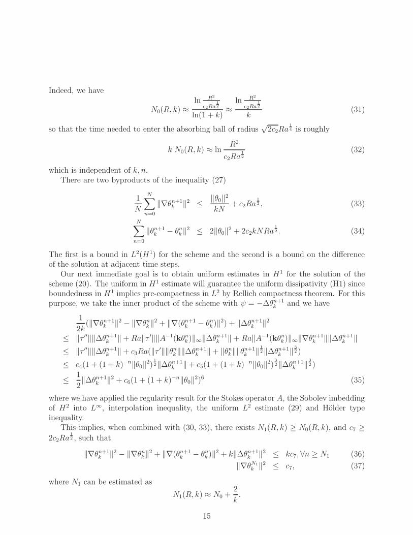
Indeed, we have

N0(R, k) ≈ln R2

c2Ra12

ln(1 + k)≈

ln R2

c2Ra12

k(31)

so that the time needed to enter the absorbing ball of radius√

2c2Ra1

4 is roughly

k N0(R, k) ≈ lnR2

c2Ra1

2

(32)

which is independent of k, n.There are two byproducts of the inequality (27)

1

N

N∑

n=0

‖∇θn+1k ‖2 ≤ ‖θ0‖2

kN+ c2Ra

1

2 , (33)

N∑

n=0

‖θn+1k − θn

k‖2 ≤ 2‖θ0‖2 + 2c2kNRa1

2 . (34)

The first is a bound in L2(H1) for the scheme and the second is a bound on the differenceof the solution at adjacent time steps.

Our next immediate goal is to obtain uniform estimates in H1 for the solution of thescheme (20). The uniform in H1 estimate will guarantee the uniform dissipativity (H1) sinceboundedness in H1 implies pre-compactness in L2 by Rellich compactness theorem. For thispurpose, we take the inner product of the scheme with ψ = −∆θn+1

k and we have

1

2k(‖∇θn+1

k ‖2 − ‖∇θnk‖2 + ‖∇(θn+1

k − θnk )‖2) + ‖∆θn+1

k ‖2

≤ ‖τ ′′‖‖∆θn+1k ‖ +Ra‖τ ′‖‖A−1(kθn

k )‖∞‖∆θn+1k ‖ +Ra‖A−1(kθn

k )‖∞‖∇θn+1k ‖‖∆θn+1

k ‖≤ ‖τ ′′‖‖∆θn+1

k ‖ + c3Ra(‖τ ′‖‖θnk‖‖∆θn+1

k ‖ + ‖θnk‖‖θn+1

k ‖ 1

2‖∆θn+1k ‖ 3

2 )

≤ c4(1 + (1 + k)−n‖θ0‖2)1

2‖∆θn+1k ‖ + c5(1 + (1 + k)−n‖θ0‖2)

3

2‖∆θn+1k ‖ 3

2 )

≤ 1

2‖∆θn+1

k ‖2 + c6(1 + (1 + k)−n‖θ0‖2)6 (35)

where we have applied the regularity result for the Stokes operator A, the Sobolev imbeddingof H2 into L∞, interpolation inequality, the uniform L2 estimate (29) and Holder typeinequality.

This implies, when combined with (30, 33), there exists N1(R, k) ≥ N0(R, k), and c7 ≥2c2Ra

1

2 , such that

‖∇θn+1k ‖2 − ‖∇θn

k‖2 + ‖∇(θn+1k − θn

k )‖2 + k‖∆θn+1k ‖2 ≤ kc7, ∀n ≥ N1 (36)

‖∇θN1

k ‖2 ≤ c7, (37)

where N1 can be estimated as

N1(R, k) ≈ N0 +2

k.

15

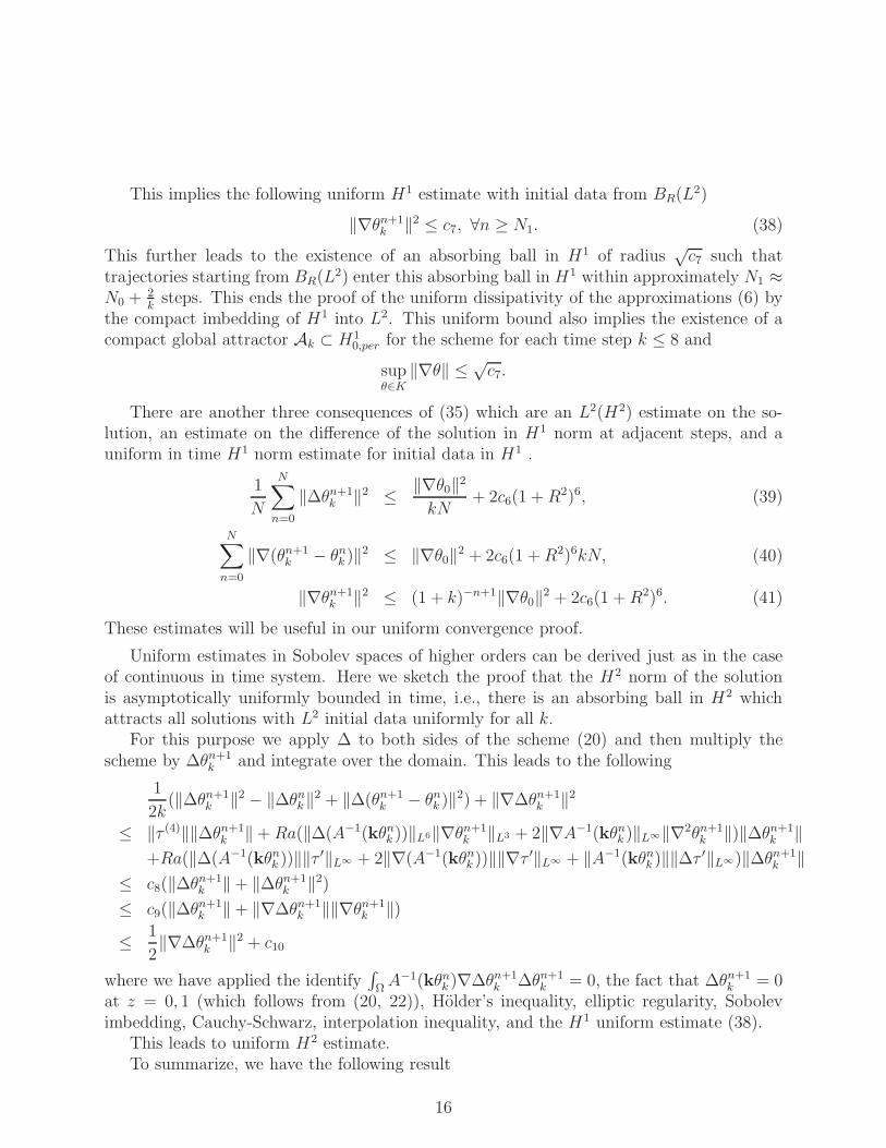
This implies the following uniform H1 estimate with initial data from BR(L2)

‖∇θn+1k ‖2 ≤ c7, ∀n ≥ N1. (38)

This further leads to the existence of an absorbing ball in H1 of radius√c7 such that

trajectories starting from BR(L2) enter this absorbing ball in H1 within approximately N1 ≈N0 + 2

ksteps. This ends the proof of the uniform dissipativity of the approximations (6) by

the compact imbedding of H1 into L2. This uniform bound also implies the existence of acompact global attractor Ak ⊂ H1

0,per for the scheme for each time step k ≤ 8 and

supθ∈K

‖∇θ‖ ≤ √c7.

There are another three consequences of (35) which are an L2(H2) estimate on the so-lution, an estimate on the difference of the solution in H1 norm at adjacent steps, and auniform in time H1 norm estimate for initial data in H1 .

1

N

N∑

n=0

‖∆θn+1k ‖2 ≤ ‖∇θ0‖2

kN+ 2c6(1 +R2)6, (39)

N∑

n=0

‖∇(θn+1k − θn

k )‖2 ≤ ‖∇θ0‖2 + 2c6(1 +R2)6kN, (40)

‖∇θn+1k ‖2 ≤ (1 + k)−n+1‖∇θ0‖2 + 2c6(1 +R2)6. (41)

These estimates will be useful in our uniform convergence proof.

Uniform estimates in Sobolev spaces of higher orders can be derived just as in the caseof continuous in time system. Here we sketch the proof that the H2 norm of the solutionis asymptotically uniformly bounded in time, i.e., there is an absorbing ball in H2 whichattracts all solutions with L2 initial data uniformly for all k.

For this purpose we apply ∆ to both sides of the scheme (20) and then multiply thescheme by ∆θn+1

k and integrate over the domain. This leads to the following

1

2k(‖∆θn+1

k ‖2 − ‖∆θnk‖2 + ‖∆(θn+1

k − θnk )‖2) + ‖∇∆θn+1

k ‖2

≤ ‖τ (4)‖‖∆θn+1k ‖ +Ra(‖∆(A−1(kθn

k ))‖L6‖∇θn+1k ‖L3 + 2‖∇A−1(kθn

k )‖L∞‖∇2θn+1k ‖)‖∆θn+1

k ‖+Ra(‖∆(A−1(kθn

k ))‖‖τ ′‖L∞ + 2‖∇(A−1(kθnk ))‖‖∇τ ′‖L∞ + ‖A−1(kθn

k )‖‖∆τ ′‖L∞)‖∆θn+1k ‖

≤ c8(‖∆θn+1k ‖ + ‖∆θn+1

k ‖2)

≤ c9(‖∆θn+1k ‖ + ‖∇∆θn+1

k ‖‖∇θn+1k ‖)

≤ 1

2‖∇∆θn+1

k ‖2 + c10

where we have applied the identify∫

ΩA−1(kθn

k )∇∆θn+1k ∆θn+1

k = 0, the fact that ∆θn+1k = 0

at z = 0, 1 (which follows from (20, 22)), Holder’s inequality, elliptic regularity, Sobolevimbedding, Cauchy-Schwarz, interpolation inequality, and the H1 uniform estimate (38).

This leads to uniform H2 estimate.To summarize, we have the following result

16

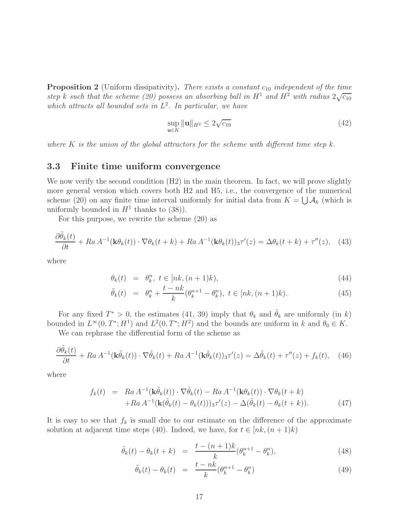
Proposition 2 (Uniform dissipativity). There exists a constant c10 independent of the timestep k such that the scheme (20) possess an absorbing ball in H1 and H2 with radius 2

√c10

which attracts all bounded sets in L2. In particular, we have

supu∈K

‖u‖H2 ≤ 2√c10 (42)

where K is the union of the global attractors for the scheme with different time step k.

3.3 Finite time uniform convergence

We now verify the second condition (H2) in the main theorem. In fact, we will prove slightlymore general version which covers both H2 and H5, i.e., the convergence of the numericalscheme (20) on any finite time interval uniformly for initial data from K =

⋃

Ak (which isuniformly bounded in H1 thanks to (38)).

For this purpose, we rewrite the scheme (20) as

∂θk(t)

∂t+RaA−1(kθk(t)) · ∇θk(t+ k) +RaA−1(kθk(t))3τ

′(z) = ∆θk(t+ k) + τ ′′(z), (43)

where

θk(t) = θnk , t ∈ [nk, (n + 1)k), (44)

θk(t) = θnk +

t− nk

k(θn+1

k − θnk ), t ∈ [nk, (n+ 1)k). (45)

For any fixed T ∗ > 0, the estimates (41, 39) imply that θk and θk are uniformly (in k)bounded in L∞(0, T ∗;H1) and L2(0, T ∗;H2) and the bounds are uniform in k and θ0 ∈ K.

We can rephrase the differential form of the scheme as

∂θk(t)

∂t+RaA−1(kθk(t)) · ∇θk(t) +RaA−1(kθk(t))3τ

′(z) = ∆θk(t) + τ ′′(z) + fk(t), (46)

where

fk(t) = RaA−1(kθk(t)) · ∇θk(t) − RaA−1(kθk(t)) · ∇θk(t+ k)

+RaA−1(k(θk(t) − θk(t)))3τ′(z) − ∆(θk(t) − θk(t+ k)). (47)

It is easy to see that fk is small due to our estimate on the difference of the approximatesolution at adjacent time steps (40). Indeed, we have, for t ∈ [nk, (n + 1)k)

θk(t) − θk(t+ k) =t− (n + 1)k

k(θn+1

k − θnk ), (48)

θk(t) − θk(t) =t− nk

k(θn+1

k − θnk ) (49)

17

and therefore, for θ0 ∈ K,

Ra‖A−1(kθk(t)) · ∇(θk(t) − θk(t+ k))‖H−1 ≤ Ra‖A−1(kθk(t))‖L∞‖θn+1k − θn

k‖≤ c11‖θn+1

k − θnk‖,

Ra‖A−1(k(θk(t) − θk(t))) · ∇θk(t+ k))‖H−1 ≤ Ra‖A−1(k(θk(t) − θk(t)))‖L∞‖θk(t+ k)‖≤ c12‖θn+1

k − θnk‖,

Ra‖A−1(k(θk(t) − θk(t))3τ′‖H−1 ≤ c13‖θn+1

k − θnk‖,

‖∆(θk(t) − θk(t+ k))‖H−1 ≤ c14‖∇(θn+1k − θn

k )‖,which further leads to

‖fk(t)‖H−1 ≤ c15‖∇(θn+1k − θn

k )‖, t ∈ [nk, (n+ 1)k) (50)

and hence, when combined with the estimate on time difference estimate (40)

‖fk‖L2(0,T ∗;H−1) ≤ c15

√

√

√

√

√

T∗

k∑

n=0

k‖∇(θn+1k − θn

k )‖2 ≤ c16√k. (51)

Taking the difference of the infinite Prandtl number model (21) and the differential formof the scheme (46), denoting ξk(t) = θ(t) − θk(t), we have

∂ξk(t)

∂t+RaA−1(kθ(t))·∇ξk(t)+RaA−1(kξk(t))·∇θk(t)+RaA

−1(kξk(t))3τ′(z) = ∆ξk(t)−fk(t).

(52)Multiplying this equation by ξk and integrating over Ω we have

1

2

d

dt‖ξk(t)‖2 + ‖∇ξk(t)‖2

≤ Ra‖A−1(kξk(t))‖L∞‖∇θk(t)‖‖ξk(t)‖ +Ra‖A−1(kξk(t))3‖L∞‖τ ′‖‖ξk(t)‖ + ‖fk(t)‖H−1‖∇ξk(t)‖

≤ c17‖ξk(t)‖2 +1

2‖fk(t)‖2

H−1 +1

2‖∇ξk(t)‖2.

Therefore we haved

dt‖ξk(t)‖2 ≤ 2c17‖ξk(t)‖2 + ‖fk(t)‖2

H−1, ‖ξk(0)‖ = 0, (53)

which leads to

‖θ − θk‖L∞(0,T ∗;L2) = ‖ξk‖L∞(0,T ∗;L2) ≤ c18‖fk‖L2(0,T ∗;H−1) ≤ c19√k → 0 (54)

uniformly for θ0 ∈ K.This ends the proof of the finite time uniform convergence which further implies H2 and

H5. To summarize, we have the following result

Proposition 3 (Finite time uniform convergence). For any T ∗ > 0, there exists a constantc19 independent of the time step k such that

‖θ(nk) − θnk‖ ≤ c19

√k, ∀θ0 ∈ K, ∀nk ≤ T ∗, (55)

i.e., assumptions H2 (7) and H5 (14) are valid for the scheme (20) with t0 = 0.

18

3.4 Finite time uniform continuity

Now we verify the finite time uniform continuity of the infinite Prandtl number model forinitial data starting from K, the union of the global attractors of the scheme with differentstep size k.

It is easy to check that the L2 norm of the infinite Prandtl number model (21) is uniformlybounded for θ0 belonging to a bounded set in L2 (see for instance [7], and the discrete version(29)). A uniform H1 norm estimate can be also derived (see (38) for the discrete version).Indeed, multiplying the infinite Prandtl number model (21) by −∆θ, integrating over Ω wededuce, for θ0 ∈ K,

1

2

d

dt‖∇θ(t)‖2 + ‖∆θ(t)‖2

≤ ‖τ”‖‖∆θ(t)‖ +Ra‖A−1(kθ(t))‖L∞‖∇θ(t)‖‖∆θ(t)‖ +Ra‖A−1(kθ(t))3‖L∞‖τ ′‖‖∆θ(t)‖≤ c20(1 + ‖θ(t)‖ + ‖θ(t)‖‖∇θ(t)‖)‖∆θ(t)‖

≤ 1

2‖∆θ(t)‖2 + c21(1 + ‖∇θ(t)‖2).

This leads to the following estimates

‖θ‖L∞(0,T ∗;H1) ≤ c22, (56)

‖θ‖L2(0,T ∗;H2) ≤ c22. (57)

Now, integrating the infinite Prandtl number model (21) in time from t to T ∗ we have,for θ0 ∈ K,

‖S(t)θ0 − S(T ∗)θ0‖

≤ |∫ T ∗

t

(‖∆θ(s)‖ +Ra‖A−1(kθ(s))‖L∞‖∇θ(s)‖ +Ra‖A−1(kθ(s))3‖L∞‖τ ′‖ + ‖τ ′′‖) ds|

≤ |∫ T ∗

t

(‖∆θ(s)‖ + c23(1 + ‖θ(s)‖‖∇θ(s)‖ + ‖θ(s)‖)) ds|

≤ |∫ T ∗

t

(‖∆θ(s)‖ + c24) ds|

≤ c25√

|T ∗ − t| (58)

where we have used elliptic regularity, the uniform H1 estimate, and the L2(H2) estimate.This completes the proof of the uniform continuity of the infinite Prandtl number model,

i.e., H3. To summarize, we have the following result

Proposition 4 (Finite time uniform continuity). For any T ∗ > 0, the infinite Prandtlnumber model (21) is continuous on the time interval [0, T ∗] uniformly for initial data fromthe union of the global attractors K defined in (6).

19

4 Conclusions and Remarks

We have presented a general/abstract result on the convergence of stationary statisticalproperties of time approximation of infinite dimensional dissipative dynamical systems. Thethree natural conditions that guarantee the convergence of the stationary statistical prop-erties of the time approximation to those of the underlying continuous in time dynamicalsystem are uniform dissipativity of the scheme for small enough time step; the convergenceof the solution to the scheme to the continuous dynamical system on the unit time interval[0, 1] uniformly for initial data from the union of the global attractors of the scheme (fordifferent time steps); and the uniform (for initial data from the union of the global attractorsof the scheme) continuity of the underlying continuous dynamical system on the unit timeinterval [0, 1]. We hope that this work will stimulate further work on numerical schemesthat are able to capture stationary statistical properties of infinite dimensional dissipativesystems.

The convergence of global attractors can be derived under the weaker assumption ofhaving a bounded union of the global attractors for the scheme. This indicates that theremight exist numerical schemes that are able to capture the global attractor asymptoticallybut not necessarily the stationary statistical properties.

We have also illustrated the application of our main result to the infinite Prandtl num-ber model for convection and we believe that the abstract main result presented here isapplicable to many other dissipative systems and associated schemes. Fully discretized ap-proximation can be studied similarly for Galerkin type spatial approximation that enjoysthe three properties postulated (see [25, 26, 10] for fully discrete long time stable schemesfor other equations). Numerical implementation in physically relevant regimes is non-trivial.Although the numerical scheme that we proposed here is linear which is advantageous overnonlinear schemes such as the one induced by the fully implicit Euler scheme proposed bymany authors, the linear equation (the matrix in the fully discretized case) changes at eachtime step due to the presence of the convection term RaA−1(kθn

k ) · ∇θn+1k . This together

with the need for long time simulation combined with the presence of physically expectedsmall spatial scales of the order of Ra−

1

3 or Ra−1

2 [2, 6, 18] which needs to be resolved makesit a challenge to simulate the physically interesting large Rayleigh number regime. One ofthe immediately goal is to design more efficient numerical scheme than the one presentedhere. We will report this and our numerical result elsewhere.

Acknowledgement

The author acknowledges helpful conversation with Andrew Majda, Jie Shen and Joe Tribbia.This work is supported in part by the National Science Foundation through DMS0606671.

20

References

[1] Billingsley, P., Weak convergence of measures: applications in probability. SIAM,Philadelphia, 1971.

[2] Chandrasekhar, S.; Hydrodynamic and hydro-magnetic stability. Oxford, ClarendonPress, 1961.

[3] Cheng, W.; Wang, X.; A Uniformly Dissipative Scheme for Stationary Statistical Prop-erties of the Infinite Prandtl Number Model, Applied Mathematics Letters, inpress. doi:10.1016/j.aml.2007.07.036

[4] Cheng, W.; Wang, X.; A semi-implicit scheme for stationary statistical properties of theinfinite Prandtl number model, SIAM J. Num. Anal., accepted July 2008.

[5] Chiu, C.; Du, Q.; Li, T.Y., Error estimates of the Markov finite approx-

imation of the Frobenius-Perron operator. Nonlinear Anal. 19(1992), no.4,291–308.

[6] Constantin, P.; Doering, C.R.; Infinite Prandtl number convection, J. Stat. Phys. 94(1999), no. 1-2, 159–172.

[7] Doering, C.R.; Otto, F.; Reznikoff, M.G., Bounds on vertical heat transport for infinitePrandtl number Rayleigh-Benard convection, J. Fluid Mech. (2006), vol. 560, pp.229-241.

[8] E, W; D. Li, The Andersen thermostat in molecular dynamics, Preprint, 2007.

[9] Foias, C., Jolly, M., Kevrekidis, I.G. and Titi,E.S., Dissipativity of numerical schemes,Nonlinearity 4 (1991), 591–613

[10] Foias, C., Jolly, M., Kevrekidis, I.G. and Titi,E.S., On some dissipative fully discretenonlinear Galerkin schemes for the Kuramoto-Sivashinsky equation, Phys. Lett. A 186

(1994), 87–96.

[11] Foias, C.; Manley, O.; Rosa, R.; Temam, R.; Navier-Stokes equations and turbulence.Encyclopedia of Mathematics and its Applications, 83. Cambridge University Press,Cambridge, 2001.

[12] Geveci, T., On the convergence of a time discretization scheme for the Navier–Stokesequations, Math. Comp., 53 (1989), pp. 43–53.

[13] Hale, J. K., Asymptotic behavior of dissipative systems, Providence, R.I. : AmericanMathematical Society, c1988.

21

[14] Heywood, J. G.; Rannacher, R.; Finite element approximation of the nonstationaryNavier-Stokes problem. II. Stability of solutions and error estimates uniform in time.SIAM J. Numer. Anal. 23 (1986), no. 4, 750–777.

[15] Hill, A.T.; Suli, E., Approximation of the global attractor for the incompressible Navier-Stokes equations, IMA J. Numer. Anal., 20 (2000), 663-667.

[16] Jones, D.A.; Stuart, A.M.; Titi, E.S., Persistence of Invariant Sets for DissipativeEvolution Equations, J. Math. Anal. Appl., 219, 479-502 (1998).

[17] Ju, N., On the global stability of a temporal discretization scheme for the Navier-Stokesequations, IMA J. Numer. Anal., 22 (2002), pp. 577–597.

[18] Kadanoff, L.P., Turbulent heat flow: structures and scaling, Physics Today, 54, no. 8,pp.34-39, 2001.

[19] Larsson, S., The long-time behavior of finite-element approximations of solutions tosemilinear parabolic problems. SIAM J. Numer. Anal. 26 (1989), no. 2, 348–365.

[20] Lasota, A.; Mackey, M.C., Chaos, Fractals, and Noise, Stochastic Aspects of Dynamics,2nd, ed. New York, Springer-Verlag, 1994.

[21] Lax, P.D., Functional Analysis, New York : Wiley, c2002.

[22] Majda, A.J.; Wang, X., Nonlinear Dynamics and Statistical Theory for Basic Geophys-ical Flows, Cambridge University Press, Cambridge, England, (2006).

[23] Monin, A.S.; Yaglom, A.M., Statistical fluid mechanics; mechanics of turbulence, En-glish ed. updated, augmented and rev. by the authors. MIT Press, Cambridge, Mass.,1975.

[24] Raugel, G., Global attractors in partial differential equations. Handbook of dynamicalsystems, Vol. 2, 885–982, North-Holland, Amsterdam, 2002.

[25] Shen, J., Convergence of approximate attractors for a fully discrete system for reaction-diffusion equations, Numer. Funct. Anal. and Optimiz., 10(11& 12) pp. 1213-1234(1989).

[26] Shen, J., Long time stabilities and convergences for the fully discrete nonlinear Galerkinmethods, Appl. Anal., 38 (1990), pp. 201–229.

[27] Stuart, A.M.; Humphries, A.R., Dynamical Systems and Numerical Analysis. Cam-bridge University Press, 1996.

[28] Temam, R.M.; Navier-Stokes Equations and Nonlinear Functional Analysis, 2nd edition,CBMS-SIAM, SIAM, 1995.

22

[29] Temam, R.M.; Infinite Dimensional Dynamical Systems in Mechanics and Physics, 2nded. Springer-Verlag, New York, 1997.

[30] Tone, F.; Wirosoetisno, D., On the long-time stability of the implicit Euler scheme forthe two-dimensional Navier-Stokes equations. SIAM J. Num. Anal. 44 (2006), no. 1,29–40

[31] Tritton, D.J.; Physical Fluid Dynamics. Oxford Science Publishing, 1988.

[32] Vishik, M.I.; Fursikov, A.V., Mathematical Problems of Statistical Hydromechanics.Kluwer Acad. Publishers, Dordrecht/Boston/London, 1988.

[33] Walters, P., An introduction to ergodic theory. Springer-Verlag, New York, 2000.

[34] Wang, X.; Infinite Prandtl Number Limit of Rayleigh-Benard Convection. Comm. Pure

and Appl. Math., vol 57, issue 10, (2004), 1265-1282.

[35] Wang, X.; Stationary statistical properties of Rayleigh-Benard convection at largePrandtl number. Comm. Pure and Appl. Math., 61 (2008), no. 6, 789–815. DOI:10.1002/cpa.20214.

[36] Wang, X.; Upper Semi-Continuity of Stationary Statistical Properties of DissipativeSystems. Dedicated to Prof. Li Ta-Tsien on the occasion of his 70th birthday. Discrete

and Continuous Dynamical Systems, A. Accepted May 2008. To appear.

23