Method of statistical spline functions for solving problems of data approximation and prediction of objects state

Serhiy Babak1[0000-0001-8805-1184], Vitaliy Babak2[0000-0002-9066-4307], Artur Zaporozhets2[0000-0002-0704-4116], Anastasia Sverdlova2[0000-0001-8222-1357]

1 University of Emerging Technologies, Kyiv, Ukraine 2 Institute of Engineering Thermophysics of NAS of Ukraine, Kyiv, Ukraine

a.o.zaporozhets@nas.gov.ua

Abstract. The method of statistical spline functions is considered for problems of predicting the state of complex technical objects using the example of power transmission lines. The choice of parameters of spline fragments for building an adequate mathematical model is analyzed. Based on the experimental data, a short-term spline forecast of heating of overhead power lines has been created.

Keywords: spline functions, mathematical model, overhead power lines, pre-diction, technical state, diagnostics

1 Introduction

The basic idea of using the mathematical apparatus of statistical spline functions for processing the spatial characteristics of a field is that some numerical characteristics of physical processes change during the observation process (meteorological fields, airspace in the vicinity of energy facilities, navigation space, etc.) for any circum-stances [1, 2, 3].

Regular observations of the history of gradual changes in these parameters over time provide an opportunity to obtain information on the trends of further changes in the studied parameters and to predict the behavior of the field at certain points [4]. For example, using the spline function algorithm, it can monitor and predict the tempera-ture at a particular point in the airspace [5]. Such a problem arises during temperature control equipment of overhead power lines (OPL) using thermal imaging equipment installed on the unmanned aerial vehicles (UAV) [6, 7].

Using the spline functions, the problem of predict ting electrical equipment failures is also solved. In this case, the main idea of predicting failures is that some numerical characteristics of physical processes occurring in certain nodes of electrical equip-ment change during the occurrence or development of faults and defects, which al-lows to identify them [8, 9]. Observations of their gradual change in time provide information on the development trends of the defect and provide a prediction of the possible moment of failure [10, 11].

In work the forecasting of values of temperature in certain points of an arrange-ment of the equipment of the OPL will be considered. Due to a significant tempera-

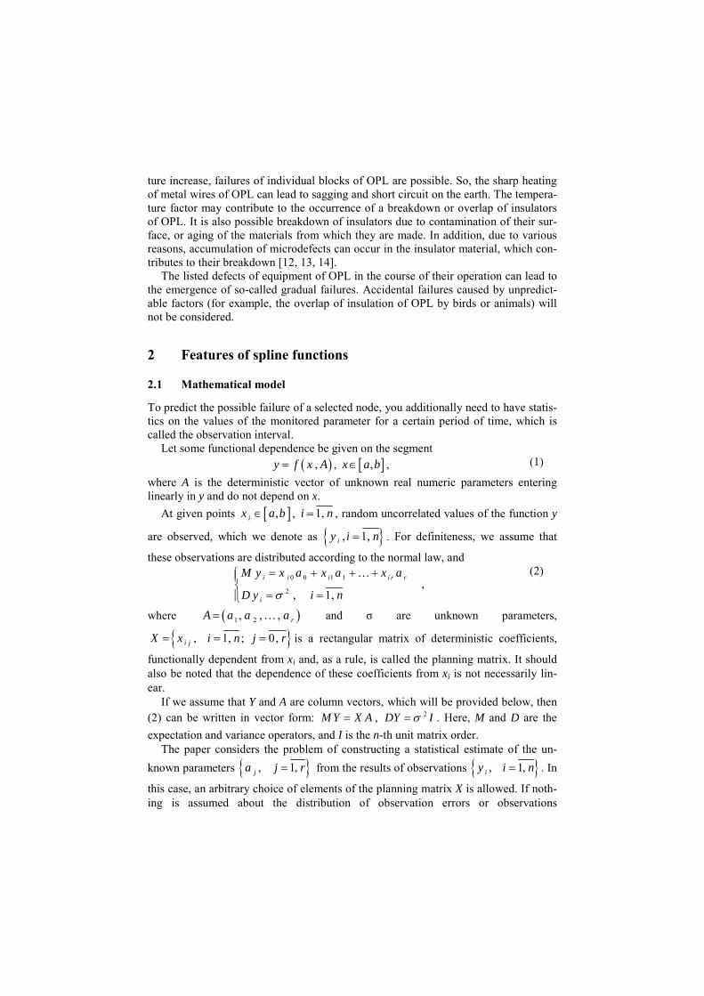
ture increase, failures of individual blocks of OPL are possible. So, the sharp heating of metal wires of OPL can lead to sagging and short circuit on the earth. The tempera-ture factor may contribute to the occurrence of a breakdown or overlap of insulators of OPL. It is also possible breakdown of insulators due to contamination of their sur-face, or aging of the materials from which they are made. In addition, due to various reasons, accumulation of microdefects can occur in the insulator material, which con-tributes to their breakdown [12, 13, 14].

The listed defects of equipment of OPL in the course of their operation can lead to the emergence of so-called gradual failures. Accidental failures caused by unpredict-able factors (for example, the overlap of insulation of OPL by birds or animals) will not be considered.

2 Features of spline functions

2.1 Mathematical model

To predict the possible failure of a selected node, you additionally need to have statis-tics on the values of the monitored parameter for a certain period of time, which is called the observation interval.

Let some functional dependence be given on the segment

,y f x A , ,x a b , (1)

where A is the deterministic vector of unknown real numeric parameters entering linearly in y and do not depend on x.

At given points ,ix a b , 1,i n , random uncorrelated values of the function y

are observed, which we denote as , 1,iy i n . For definiteness, we assume that

these observations are distributed according to the normal law, and

0 0 1 1

2,

, 1,

i i i i r r

i

M y x a x a x a

D y i n

(2)

where 1 2, , , rA a a a and σ are unknown parameters,

, 1, ; 0,i jX x i n j r is a rectangular matrix of deterministic coefficients,

functionally dependent from xi and, as a rule, is called the planning matrix. It should also be noted that the dependence of these coefficients from xi is not necessarily lin-ear.

If we assume that Y and A are column vectors, which will be provided below, then (2) can be written in vector form: M Y X A , 2DY I . Here, M and D are the

expectation and variance operators, and I is the n-th unit matrix order. The paper considers the problem of constructing a statistical estimate of the un-

known parameters , 1,ja j r from the results of observations , 1,iy i n . In

this case, an arbitrary choice of elements of the planning matrix X is allowed. If noth-ing is assumed about the distribution of observation errors or observations

, 1,iy i n , then as a result of solving this problem the largest, what can we ex-

pect, is the construction of point estimates for elements A. Under the assumption that the distribution law of observations is normal, we can obtain a confidence interval for the estimated parameters.

Considering that in the task set the question of introducing the planning matrix is solved in an arbitrary way, we specify this task by refining the choice of the planning matrix X. At the same time, we construct statistical estimates of the A parameters using the least squares method, which in the case of normally distributed yi leads to the same result as maximum likelihood estimation.

Concretization in the choice of the planning matrix, first of all, is connected with the choice of the upcoming functions. The task was traditionally solved in the class of polynomials. But polynomial approximations have several disadvantages, the most significant of which is that the sequence of interpolation polynomials does not always converge to the interpolated function. Therefore, in many problems, the more natural and convenient approximation apparatus turned out to be splines, with the help of which we will solve the problem posed.

Splines are functions that are “glued together” from pieces of various functions in a specific pattern. Polynomial splines “stick together” from pieces of various polynomi-als in such a way as to ensure the necessary smoothness of the resulting spline. The simplest example of a polynomial spline is a broken line.

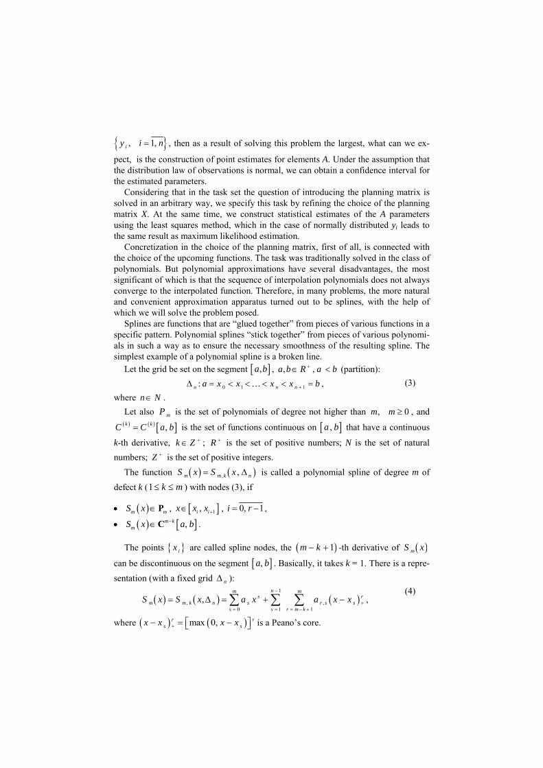
Let the grid be set on the segment ,a b , , ,a b R a b (partition):

0 1 1:n n na x x x x b , (3)

where n N .

Let also mP is the set of polynomials of degree not higher than , 0m m , and ,k kC C a b is the set of functions continuous on ,a b that have a continuous

k-th derivative, k Z ; R is the set of positive numbers; N is the set of natural

numbers; Z is the set of positive integers.

The function , ,m m k nS x S x is called a polynomial spline of degree m of

defect k (1 k m ) with nodes (3), if

m mS x P , 1,i ix x x , 0, 1i r ,

,m kmS x a bC .

The points ix are called spline nodes, the 1m k -th derivative of mS x

can be discontinuous on the segment ,a b . Basically, it takes k = 1. There is a repre-

sentation (with a fixed grid n ):

1

, ,0 1 1

,nm m

s rm m k n s r s s

s s r m k

S x S x a x a x x

, (4)

where max 0,r rs sx x x x is a Peano’s core.

The coefficients sa and ,r sa can take arbitrary values from R; the set

, ,m k nS x with a fixed n is linear with dimension 1m nk . Therefore, for an

unambiguous definition of a spline, it is necessary to specify 1m nk independent

conditions. For a linear spline this is 2n , that is, for the statistics obtained, the

number of parameters that need to be estimated is found from condition 2r n .

Thus, under the conditions of the formulated problem, it is necessary on the seg-

ment ,a b for given r to find a grid rjx such that the spline

1 ,kkS x a b C , 0,1, ,k constructed on the grid r provides the minimum

(in terms of standard quadratic deviations) statistical estimate of the vector A, that is, we assume that

1 1 11

r

i i r k ij

x a x S x

, 1,i n . (5)

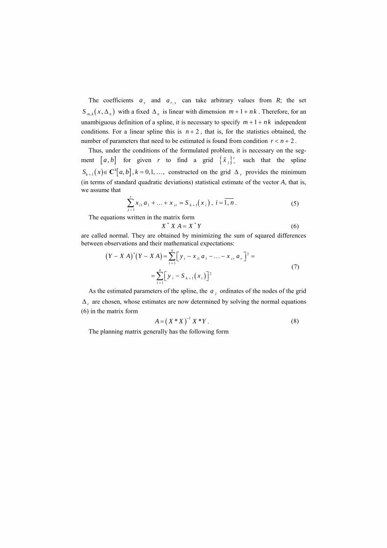
The equations written in the matrix form * *X X A X Y (6)

are called normal. They are obtained by minimizing the sum of squared differences between observations and their mathematical expectations:

* 21 1

1

21

1

n

i i i r ri

n

i k ii

Y X A Y X A y x a x a

y S x

(7)

As the estimated parameters of the spline, the ja ordinates of the nodes of the grid

r are chosen, whose estimates are now determined by solving the normal equations

(6) in the matrix form

1* *A X X X Y

. (8)

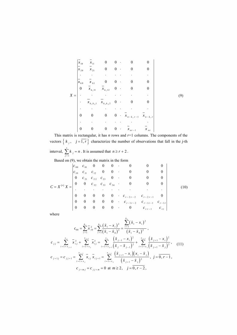
The planning matrix generally has the following form

1 1

1 2 1 2

10 11

20 21

0 1

11 12

1 2

1

1

0 0 0 0

0 0 0 0

0 0 0 0

0 0 0 0

0 0 0

0 0 0 0

0 0 0 0

r r

k k

k k

k k k k

n k r n k r

n r n r

x x

x x

x x

x x

X

x x

x x

x x

(9)

This matrix is rectangular, it has n rows and r+1 columns. The components of the

vectors , 1,jk j r characterize the number of observations that fall in the j-th

interval, 1

r

jj

k n

. It is assumed that 2n r .

Based on (9), we obtain the matrix in the form

00 01

10 11 12

21 2 2 23

32 33 34

2 2 2 1

1 2 1 1 1

1

0 0 0 0 0 0

0 0 0 0 0

0 0 0 0 0

0 0 0 0 0

0 0 0 0 0 0

0 0 0 0 0

0 0 0 0 0 0

r r r r

r r r r r r

r r r r

c c

c c c

c c c

c c cC X X

c c

c c c

c c

(10)

where

1

1 1

212

11200 0 2 2

1 1 1 0 1 0

k

ik kii

ii i

x xx x

c xx x x x

,

1 1

1 1

2 21 12 2

2 21 1 1 11 1

j jj j

j j j j

s ss sj i j i

j j i j i ji s i s i s i sj j j j

x x x xc x x

x x x x

,

1 11

1 1 1 21 1 1

j j

j j

s sj i i j

j j j j i j i ji s i s j j

x x x xc c x x

x x

, 0, 1j r ,

0j m j j j mc c at 2, 0, 2m j r ,

(11)

212

21 1 1r r

n nr i

r r i ri n k i n k r r

x xc x

x x

,

and ix are the elements of the source data (experimental points), 1

j

j mm

S k

,

1 ,j r , 0 0, rs s n . The matrix C is rectangular 1 1r r .

The above relations are obtained by directly multiplying the matrices X and X

with (9) taken into account. Let us briefly discuss some properties of the matrix C.

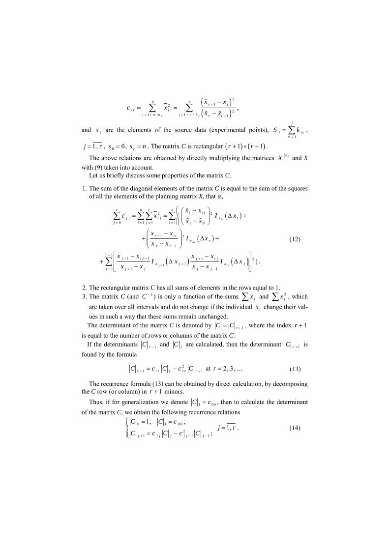
1. The sum of the diagonal elements of the matrix C is equal to the sum of the squares of all the elements of the planning matrix X, that is,

1

1

1 12 21

0 1 1 1 1 0

1 2

1

11 1 1 2

11 1 1

}.

i

ii r

i j i j

r n r ni

j j i j xj i j i

r i rx r

r r

rj i j j i j

x j x jj j j j j

x xc x I x

x x

x xI x

x x

x x x xI x I x

x x x x

(12)

2. The rectangular matrix C has all sums of elements in the rows equal to 1. 3. The matrix C (and 1C ) is only a function of the sums ix and 2

ix , which

are taken over all intervals and do not change if the individual ix change their val-

ues in such a way that these sums remain unchanged. The determinant of the matrix C is denoted by 1rC C , where the index 1r

is equal to the number of rows or columns of the matrix C. If the determinants 1rC and rC are calculated, then the determinant 1rC is

found by the formula

21 1r r r r r r rC c C c C at 2, 3,r (13)

The recurrence formula (13) can be obtained by direct calculation, by decomposing the C row (or column) in 1r minors.

Thus, if for generalization we denote 1 00C c , then to calculate the determinant

of the matrix C, we obtain the following recurrence relations

0 1 00

21 1 1

1; ;

;j j j j j j j

C C c

C c C c C

1,j r . (14)

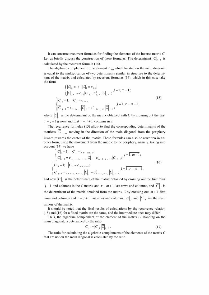
It can construct recurrent formulas for finding the elements of the inverse matrix C. Let us briefly discuss the construction of these formulas. The determinant 1rC is

calculated by the recurrent formula (14). The algebraic complement of the element minc which located on the main diagonal

is equal to the multiplication of two determinants similar in structure to the determi-nant of the matrix and calculated by recurrent formulas (14), which in this case take the form

0 1 00

21 1 1

1; ;

;j j j j j j j

C C c

C c C c C

1, 1j m ;

0 1

21 1 1

1; ;

;

r r

j r j r j j r j r j j

C C c

C c C c C

1 , 1 ,j r m

(15)

where jC is the determinant of the matrix obtained with C by crossing out the first

1r j g rows and first 1r j columns in it.

The recurrence formulas (15) allow to find the corresponding determinants of the

matrices r mC moving in the direction of the main diagonal from the periphery

inward towards the center of the matrix. These formulas can also be rewritten in an-other form, using the movement from the middle to the periphery, namely, taking into account (14) we have

0 1 1 1

21 1 1 1 1

1; ;

;

m m

j m j m j j m j m j j

C C c

C c C c C

1, 1j m ;

0 1 1 1

21 1 1 1 1

1; ;

;

m m

j m j m j j m j m j j

C C c

C c C c C

1 , 1 ,j r m

(16)

and now jC is the determinant of the matrix obtained by crossing out the first rows

1j and columns in the C matrix and 1r m last rows and columns, and jC is

the determinant of the matrix obtained from the matrix C by crossing out 1m first

rows and columns and 1r j last rows and columns, jC and jC are the main

minors of the matrix. It should be noted that the final results of calculations by the recurrence relation

(15) and (16) for a fixed matrix are the same, and the intermediate ones may differ. Thus, the algebraic complement of the element of the matrix C, standing on the

main diagonal, is determined by the ratio

1j j j rC C C . (17)

The ratio for calculating the algebraic complements of the elements of the matrix C that are not on the main diagonal is calculated by the ratio

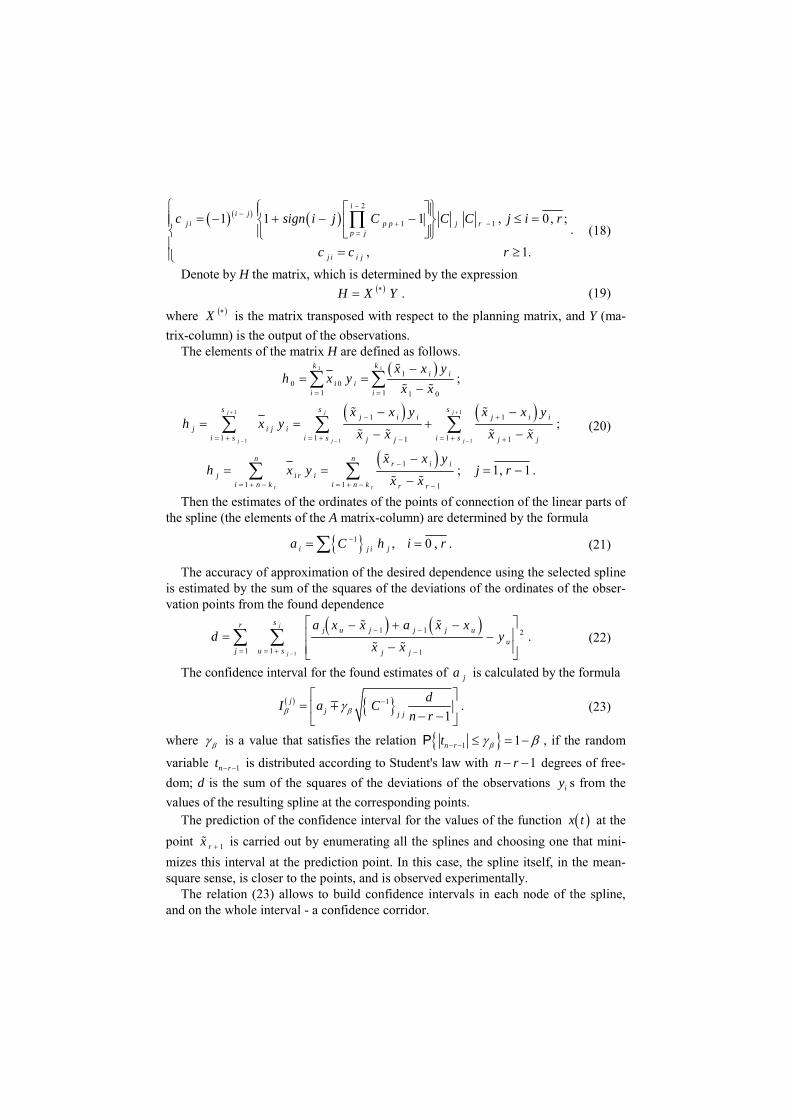
2

1 11 1 1 , 0, ;

, 1.

ii j

j i p p j rp j

j i i j

c sign i j C C C j i r

c c r

. (18)

Denote by H the matrix, which is determined by the expression H X Y . (19)

where X is the matrix transposed with respect to the planning matrix, and Y (ma-

trix-column) is the output of the observations. The elements of the matrix H are defined as follows.

1 11

0 01 1 1 0

k ki i

i ii i

x x yh x y

x x

;

1 1

1 1 1

1 1

1 1 11 1

j jj

j j j

s ssj i i j i i

j i j ii s i s i sj j j j

x x y x x yh x y

x x x x

;

1

1 1 1

; 1, 1r r

n nr i i

j i r ii n k i n k r r

x x yh x y j r

x x

.

(20)

Then the estimates of the ordinates of the points of connection of the linear parts of the spline (the elements of the A matrix-column) are determined by the formula

1 , 0 ,i j i ja C h i r . (21)

The accuracy of approximation of the desired dependence using the selected spline is estimated by the sum of the squares of the deviations of the ordinates of the obser-vation points from the found dependence

1

1 1 2

1 1 1

j

j

srj u j j j u

uj u s j j

a x x a x xd y

x x

. (22)

The confidence interval for the found estimates of ja is calculated by the formula

11

jj j j

dI a C

n r

. (23)

where is a value that satisfies the relation 1 1n rt P , if the random

variable 1n rt is distributed according to Student's law with 1n r degrees of free-

dom; d is the sum of the squares of the deviations of the observations iy s from the

values of the resulting spline at the corresponding points. The prediction of the confidence interval for the values of the function x t at the

point 1rx is carried out by enumerating all the splines and choosing one that mini-

mizes this interval at the prediction point. In this case, the spline itself, in the mean-square sense, is closer to the points, and is observed experimentally.

The relation (23) allows to build confidence intervals in each node of the spline, and on the whole interval - a confidence corridor.

To obtain a forecast using a statistical spline, an additional node is introduced to the set of nodes of the spline, the abscissa of which corresponds to the forecast inter-val. Using a computer search method, a grid is selected that satisfies equation (8) and at the same time minimizes it on the set of possible non-uniform grids and the width of the confidence interval in the forecast node.

As a result, the expected value and the confidence interval for the selected con-trolled parameter at the end of the forecast interval will be obtained. The boundaries of the confidence corridor are formed by linear interpolation of the upper and lower boundaries of the confidence intervals in all nodes of the resulting spline, including the forecast node.

2.2 Experimental results

Based on the considered spline forecast method, algorithms are built and a com-puter program is developed that implements this method. It is a computer program that is the main part of the proposed method, which makes it possible to carry out a short-term forecast for determining the time interval in which the temperature of the OPL can reach critical values. All the basic information about this program, practical issues of its application are set out in the work, as well as in special documentation.

The application of the proposed method for constructing a forecast will be consid-ered on a specific example.

For the implementation of such a forecast, it was necessary, first of all, to obtain experimental statistical data on the temperature state of the wires of OPL. In addition, the initial data for the program are:

the number of temperature measurements 11n (in our case);

the number of hours of the forecast 3forn ;

the number of intervals, interpolates spline 5r ;

the number of intervals of the time interval, on which the temperature is measured (the breakdown is performed in order to find the optimal interpolation spline),

10breakn ;

confidence probability of estimating the prediction of the length of the time inter-val to reach the critical temperature of the power lines, 0.95P .

As a result of the calculation of the program we obtain the data that are presented in Table 1 and in Fig. 1.

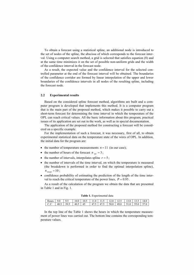
Table 1. Experimental data

Hours 9.0 9.5 10.0 10.5 11.0 11.5 12.0 12.5 13.0 13.5 14.0 to, C 40.5 39.5 40.5 45 47.5 47.5 50.0 49.0 51.0 55.0 57.0

In the top line of the Table 1 shows the hours in which the temperature measure-

ment of power lines was carried out. The bottom line contains the corresponding tem-perature values.

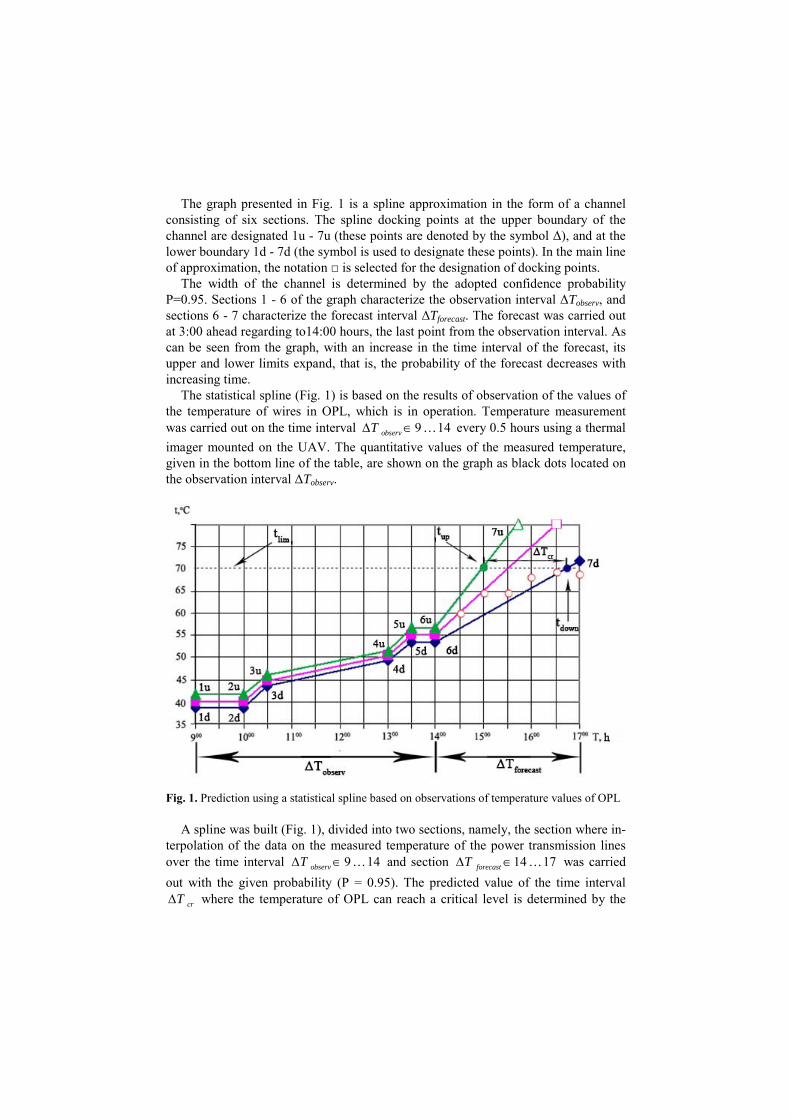
The graph presented in Fig. 1 is a spline approximation in the form of a channel consisting of six sections. The spline docking points at the upper boundary of the channel are designated 1u - 7u (these points are denoted by the symbol Δ), and at the lower boundary 1d - 7d (the symbol is used to designate these points). In the main line of approximation, the notation □ is selected for the designation of docking points.

The width of the channel is determined by the adopted confidence probability P=0.95. Sections 1 - 6 of the graph characterize the observation interval ΔTobserv, and sections 6 - 7 characterize the forecast interval ΔTforecast. The forecast was carried out at 3:00 ahead regarding to14:00 hours, the last point from the observation interval. As can be seen from the graph, with an increase in the time interval of the forecast, its upper and lower limits expand, that is, the probability of the forecast decreases with increasing time.

The statistical spline (Fig. 1) is based on the results of observation of the values of the temperature of wires in OPL, which is in operation. Temperature measurement was carried out on the time interval 9 14observT every 0.5 hours using a thermal

imager mounted on the UAV. The quantitative values of the measured temperature, given in the bottom line of the table, are shown on the graph as black dots located on the observation interval ΔTobserv.

Fig. 1. Prediction using a statistical spline based on observations of temperature values of OPL

A spline was built (Fig. 1), divided into two sections, namely, the section where in-terpolation of the data on the measured temperature of the power transmission lines over the time interval 9 14observT and section 14 17forecastT was carried

out with the given probability (P = 0.95). The predicted value of the time interval

crT where the temperature of OPL can reach a critical level is determined by the

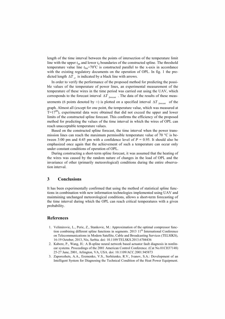
length of the time interval between the points of intersection of the temperature limit line with the upper tup and lower td boundaries of the constructed spline. The threshold temperature value line tlim=70oC is constructed parallel to the x-axis in accordance with the existing regulatory documents on the operation of OPL. In fig. 1 the pre-dicted length crT is indicated by a black line with arrows.

In order to verify the performance of the proposed method for predicting the possi-ble values of the temperature of power lines, an experimental measurement of the temperature of these wires in the time period was carried out using the UAV, which corresponds to the forecast interval forecastT . The data of the results of these meas-

urements (6 points denoted by ○) is plotted on a specified interval forecastT of the

graph. Almost all (except for one point, the temperature value, which was measured at T=1700), experimental data were obtained that did not exceed the upper and lower limits of the constructed spline forecast. This confirms the efficiency of the proposed method for predicting the values of the time interval in which the wires of OPL can reach unacceptable temperature values.

Based on the constructed spline forecast, the time interval when the power trans-mission lines can reach the maximum permissible temperature value of 70 °C is be-tween 3:00 pm and 4:45 pm with a confidence level of P = 0.95. It should also be emphasized once again that the achievement of such a temperature can occur only under constant conditions of operation of OPL.

During constructing a short-term spline forecast, it was assumed that the heating of the wires was caused by the random nature of changes in the load of OPL and the invariance of other (primarily meteorological) conditions during the entire observa-tion interval.

3 Conclusions

It has been experimentally confirmed that using the method of statistical spline func-tions in combination with new information technologies implemented using UAV and maintaining unchanged meteorological conditions, allows a short-term forecasting of the time interval during which the OPL can reach critical temperatures with a given probability.

References

1. Velimirovic, L., Peric, Z., Stankovic, M.: Approximation of the optimal compressor func-tion combining different spline functions in segments. 2013 11th International Conference on Telecommunications in Modern Satellite, Cable and Broadcasting Services (TELSIKS), 16-19 October, 2013, Nis, Serbia. doi: 10.1109/TELSKS.2013.6704436

2. Kabore, P., Wang, H.: A B-spline neural network based actuator fault diagnosis in nonlin-ear systems. Proceedings of the 2001 American Control Conference. (Cat No.01CH37148) 25-27 June, 2001, Arlington, VA, USA. doi: 10.1109/ACC.2001.945873

3. Zaporozhets, A.A., Eremenko, V.S., Serhiienko, R.V., Ivanov, S.A.: Development of an Intelligent System for Diagnosing the Technical Condition of the Heat Power Equipment.

2018 IEEE 13th International Scientific and Technical Conference on Computer Sciences and Information Technologies (CSIT), 11-14 September, 2018, Lviv, Ukraine. doi: 10.1109/STC-CSIT.2018.8526742

4. Zaporozhets, A., Redko, O., Babak, V., Eremenko, V., Mokiychuk, V.: Method of indirect measurement of oxygen concentration in the air. Naukovyi Visnyk Natsionalnoho Hirny-choho Universytetu, 2018, №5, pp. 105-114. doi: 10.29202/nvngu/2018-5/14

5. Yao, L., Guan, Y.: Minimum entropy fault diagnosis and fault tolerant control for the non-Gaussian stochastic system. 2016 American Control Conference (ACC). 6-8 July, 2016, Boston, MA, USA. doi: 10.1109/ACC.2016.7526753

6. Peng, X., Qian, G., Li, X., Gao, F.: Intelligent trip-out fault diagnosis of overhead trans-mission line. High Voltage Engineering, 2012, Vol. 38, Issue 8, pp. 1965-1972.

7. Li, P., Li, Q., Cao, M., Gao, S., Huang, H.: Time series prediction for icing process of overhead power transmissions line based on BP neural networks. Proceedings of the 30th Chinese Control Conference. 22-24 July, 2011, Yantai, China.

8. Kuts, Y., Eremenko, V., Monchenko, E., Protasov, A.: Ultrasound method of multi-layer material thickness measurement. AIP Conference Proceedings 1096, 2009, Vol. 1115. doi: 10.1063/1.3114079

9. Zaporozhets, A., Eremenko, V., Serhiienko, R., Ivanov, S.: Methods and Hardware for Dianosing Thermal Power Equipment Based on Smart Grid Technology, Advances in Intelligent Systems and Computing III, 2019, Vol. 871, pp. 476-492. doi: 10.1007/978-3-030-01069-0_34

10. Babak., V., Mokiychuk, V., Zaporozhets, A., Redko, O.: Improving the efficiency of fuel combustion with regard to the uncertainty of measuring oxygen concentration. Eastern-European Journal of Enterprise Technologies, 2016, Vol. 6, №8, pp. 54-59. doi: 10.15587/1729-4061.2016.85408

11. Klevtsov, S.: Identification of the state of technical objects based on analyzing a limited set of parameters. 2016 International Siberian Conference on Control and Communications (SIBCON), 12-14 May, 2016, Moscow, Russia. doi: 10.1109/SIBCON.2016.7491752

12. Manusov, V.Z., Orlov, D.V., Frolova, V.V.: Diagnostic of Technical State of Modern Transformer Equipment Using the Analytical Hierarchy Process. 2018 IEEE International Conference on Environment and Electrical Engineering and 2018 IEEE Industrial and Commercial Power Systems Europe (EEEIC / I&CPS Europe), 12-15 June, 2018, Palermo, Italy. doi: 10.1109/EEEIC.2018.8493904

13. Ming, J., Zhang, L., Sun, J., Zhang, Y.: Analysis models of technical and economic data of mining enterprises based on big data analysis. 2018 IEEE 3rd International Conference on Cloud Computing and Big Data Analysis (ICCCBDA), 20-22 April, 2018, Chengdu, China. doi: 10.1109/ICCCBDA.2018.8386516

14. Dmitriev, S., Manusov, V., Ahyoev, J.: Diagnosing of the current technical condition of electric equipment on the basis of expert models with fuzzy logic. 2016 57th International Scientific Conference on Power and Electrical Engineering of Riga Technical University (RTUCON), 13-14 October, 2016, Riga, Latvia. doi: 10.1109/RTUCON.2016.7763126