Approximation Algorithms for Developable

Surfaces

Helmut Pottmann and Johannes WallnerInstitut fur Geometrie, Technische Universitat WienWiedner Hauptstraße 8–10, A–1040 Wien, Austria

Abstract

By its dual representation, a developable surface can be viewed as a curve

of dual projective 3-space. After introducing an appropriate metric in the

dual space and restricting ourselves to special parametrizations of the sur-

faces involved, we derive linear approximation algorithms for developable

NURBS surfaces, including multiscale approximations. Special attention

is paid to controlling the curve of regression.

Keywords: computer aided geometric design, surface approximation, de-

velopable surface, dual representation, NURBS

1 Introduction

A developable surface is a surface which can be unfolded (developed) into a planewithout stretching or tearing. Mathematically speaking, there is a mapping ofthe surface into the Euclidean plane which is isometric, at least locally. Becauseof this property, developable surfaces possess a variety of applications in man-ufacturing with materials that are not amenable to stretching. These includethe formation of aircraft skins, ship hulls, ducts and automobile parts such asupholstery, body panels and windshields (see e.g. [8]).

Since current CAD/CAM systems are using rational B-splines (NURBS) asstandard for curve and surface representations [7, 18], there is a demand forefficient computing with developable NURBS surfaces. There are basically twoapproaches to dealing with rational developable surfaces. On the one hand, onecan express such a surface as a tensor product surface of degree (1, n) and solvethe nonlinear side conditions expressing the developability [1, 2, 5, 14]. On theother hand, we can view the surface as envelope of its one parameter set of tangentplanes and thus treat it as a curve in dual projective space [3, 4, 11, 12, 19, 20].Based on the latter approach, some interpolation and approximation algorithms

1

as well as initial solutions to special applications have been presented recently[11, 12, 13, 20, 22, 24]

In the present paper we develop further the use of the dual representation forthe solution of fundamental approximation problems with developable surfaces.The new algorithms are based on appropriate metrics in dual space as well as onlimitation to special surface classes. Thus most of them are of a linear nature.Only pushing out the line of regression from the area of interest requires thesolution of convex programming problem.

2 The dual representation of developable sur-

faces

Developable surfaces can be isometrically mapped (developed) into the plane, atleast locally. When sufficient differentiability is assumed, they are characterizedby the vanishing of their Gaussian curvature. A non-flat developable surface isthe envelope of its one parameter family of tangent planes. Such a developablesurface locally is either a conical surface, a cylindrical surface, or the tangentsurface of a twisted curve. Globally, of course, it can be a rather complicatedcomposition of these three surface types. Thus, developable surfaces are ruledsurfaces, but with the special property that they possess the same tangent planeat all points of the same generator (=ruling).

We will do our calculations in the projective extension P 3 of real Euclidean3-space E3 and use homogeneous Cartesian coordinates (x0, x1, x2, x3) for points.For points not at infinity, i.e., x0 6= 0, the corresponding inhomogeneous Cartesiancoordinates will be denoted by

x =x1

x0

, y =x2

x0

, z =x3

x0

;

we write X = (x, y, z).A plane with equation u0x0 + u1x1 + u2x2 + u3x3 = 0, or, equivalently, u0 +

u1x + u2y + u3z = 0 can be represented by its homogeneous plane coordinatesU = (u0, u1, u2, u3).

Because in all points of a generator line the tangent plane is the same, wecan identify a developable surface with the one-parameter family of its tangentplanes U(t), or in other words, with a certain curve in dual projective space. Ifthis curve is a NURBS curve

U(t) =n∑

i=0

UiNki (t), (1)

we call the original surface a developable NURBS surface. Here the N ki denote

normalized B-spline basis functions of degree k over a given knot vector. The

2

word ‘normalized’ means that the sum of the basis functions is the constantfunction 1. The symbol Ui denotes a coordinate quadruple of the i-th controlplane Ui. Of course the coordinate quadruple contains more information thanjust the plane as a point set, but for simplicity we just speak of the coordinatesof the plane.

There is no mathematical reason why we restrict ourselves to the B-splines.They have, however, a lot of properties which make them easy to deal with. Atheorem is easily verified to hold for developable surfaces which are modeled bya different spline space as well, if this spline space enjoys all properties of theB-spline space which are used in the proof of this theorem.

It is well known that the plane U(t) touches the envelope of the family U(t)along the generator line

U(t) ∩ U(t).

In particular, the rulings which correspond to parameter values which are (k+1)-fold knots (usually t0 and tn), can easily be expressed in terms of the controlplanes.

The cuspoidal edge or line of regression of the surface is obtained as theintersection

U(t) ∩ U(t) ∩ U(t).

In general it is a rational B-spline curve of degree 3k − 6.Recently, algorithms for the computation with the dual representation, the

conversion to the standard tensor product representation and the solution of in-terpolation and some approximation algorithms have been developed [11, 12, 20].In this paper we explore further approximation of and with developable surfaces.This is not a straightforward application of duality, as might be expected, sinceduality does not extend to the Euclidean metric and, moreover, Euclidean geom-etry does not contain deviation measures between planes that would be useful inthe present context.

3 A special class of developable NURBS sur-

faces

3.1 Definitions and elementary properties

For the approximation algorithms discussed in this paper, we will restrict theclass of developable surfaces we are working with: We only consider surfaceswhose family of tangent planes is of the form

U(t) = (u0(t), u1(t), u2(t),−1). (2)

For NURBS surfaces this is equivalent to the choice of control planes Ui = (u0,i,u1,i, u2,i, u3,i) such that always u3,i = −1. This means that for all possible planes

3

U we no longer allow to choose an arbitrary coordinate quadruple describing U ,but we restrict ourselves to the unique one whose last coordinate equals −1. Thisis not possible if the last coordinate is zero, so we have to exclude all surfaceswith tangent planes parallel to the z-axis. In most cases this requirement is easilyfulfilled by choosing an appropriate coordinate system.

We can also use other basis functions (instead of the normalized B-splines),which do not sum up to 1. The only difference is that we have to set u3(t) to −1and to ignore the third coordinate of planes when computing ui(t). This makesthe formulae more clumsy, but is no essential restriction.

Dual projective space with the bundle of planes (u0, u1, u2, 0) removed is anaffine space and (u0, u1, u2), describing the plane (u0, u1, u2,−1), are affine coor-dinates in it. The surfaces (2) become ordinary piecewise polynomial B-splinecurves.

For most applications it is convenient to restrict the class of surfaces evenfurther by prescribing the parametrization:

U(t) = (u0(t), u1(t), t,−1). (3)

Its generators g(t) lie in the first derivative planes, which now have the form

U(t) = (u0, u1, 1, 0) (4)

As it was with the surfaces of type (2), it does not matter whether or not thespline space contains the identity function t 7→ t. The set of parametrizations(u0(t), u1(t), t,−1) with u0 and u1 from our spline space still is a well-defined setof functions whose properties can be studied, and which metrics of an ambientspace can be restricted to (see later).

The next lemma shows some limitations of the class (3):

Lemma 1 The surfaces (3) do not possess inflection generators and generatorsparallel to the plane x = 0.

Proof: The generator g(t0) is an inflection generator if and only if U(t) has asingularity as a curve in projective space. For surfaces of type (2) this happensif and only if U(t) = 0, and it never happens for surfaces of type (3).

Further, direct calculation gives the intersection point of the three planesU(t), U(t) and x = 0, which never is situated at infinity. 2

Because inflection generators are singularities in dual space, they need a spe-cial treatment anyway. In approximation problems we will have to cut the surfacewhich we want to approximate into pieces which do not contain inflection gen-erators. For a detailed study of inflection generators of developable surfaces inconnection with applications in manufacturing, we refer the reader to [6].

For more insight into the geometry of the special developable surfaces of type(3), let us intersect the surface with the plane x = c.

4

Lemma 2 The intersection curve Cc of a NURBS surface (3) with the planex = c is a polynomial B-spline curve of degree k and knot multiplicities onegreater than the knot multiplicities of (3).

Proof: The curve Cc is the envelope of the lines z = u0 + cu1 + ty. Thus thegeometric meaning of the parameter t is the tangent slope of the intersectioncurves Cc. An elementary calculation gives the parametric representation of Cc:

x = c, y = −hc(t), z = hc(t) − thc(t), with hc(t) := u0(t) + cu1(t). (5)

We see that these are polynomial B-spline curves. The function thc is of polyno-mial degree less or equal k and its differentiability class at the knot values is oneless then the differentiability class of the ui. This implies the statement aboutthe multiplicities. 2

Corollary 3 A developable NURBS surface (3) can also be written as a polyno-mial tensor product B-spline surface of degree (1, k),

S = (1 − u)Ca(t) + uCb(t),

where Ca and Cb are the intersection curves in planes x = a and x = b.

Developable tensor product B-spline surfaces with boundary curves in parallelplanes have been investigated in several papers [1, 2, 5], but the computationalsimplicity of our special subclass (3) remained unobserved so far.

4 Approximation algorithms

Our treatment of approximation problems is based on two ingredients. First, weare limiting our candidate surfaces which we would like to use for approximationto special subclasses discussed in the previous section. Second, we are usingappropriate error measures, which will be discussed now.

4.1 Distance functions between planes

In order to approximate a given set of planes by another one, it is necessaryto introduce an appropriate distance between two planes. Euclidean geometrydoes not directly provide such a distance function. All invariants are expressedin terms of the angle between planes and are inappropriate for our purposes,because we are only interested in the distances of points of the two planes whichare near some region of interest, and this distance can become arbitrarily largewith the angle getting arbitrarily close to zero at the same time.

In order to keep certain algorithms linear, we approach the problem in thefollowing way. When designing a developable surface, we do it in pieces for which

5

there exists a vector e ∈ R3 such that the angle between the surface normals and

e does not exceed some angle γ0 < π/2. Then, e is taken as third unit vectorof a Cartesian coordinate system. Now all tangent planes of the surface can bewritten as graph of a linear function in x and y as z = u0 + u1x + u2y.

For a positive measure µ in R2 we define the distance dµ between planes

Ui = (u0,i, u1,i, u2,i,−1) as

dµ(U1, U2) = ‖(u0,1 − u0,2) + (u1,1 − u1,2)x + (u2,1 − u2,2)y‖L2(µ), (6)

i.e., the L2(µ)-distance of the linear functions whose graphs are U1 and U2. This,of course, makes sense only if the linear function which represents the differencebetween the two planes is in L2(µ). We will always assume that the measure µis such that all linear and quadratic functions possess finite integral.

A useful choice for µ is Lebesgue measure dxdy times the characteristic func-tion of a region of interest. If µ = dxdyχD, we have

dµ(U1, U2)2 =

∫

D

((u0,1 − u0,2) + (u1,1 − u1,2)x + (u2,1 − u2,2)y)2dxdy. (7)

We write dD(U1, U2) instead of dµ(U1, U2).Another possibility is that µ equals the sum of several point masses at points

(xi, yi), see [11]. In this case we have

dµ(U1, U2)2 =

∑

j

((u0,1 − u0,2) + (u1,1 − u1,2)xj + (u2,1 − u2,2)yj)2. (8)

Lemma 4 The distance dµ defines a Euclidean metric in the set of planes of type(2), if and only if µ is not concentrated in a straight line.

Proof: The coefficients of the planes enter (7) in a bilinear way. Symmetry andpositive semi-definiteness follow from the respective properties of the L2 scalarproduct. The positive definiteness is also seen easily:

Suppose the zero set of the nonzero linear function f(x, y) the line g. µ isnot concentrated on g, so there is a measurable set E with µ(E \ g) > 0. LetAn = {P ∈ R

2|2−(n+1) ≤ Pg < 2−n}. Then µ(E \ g) =∑

n∈Zµ(E ∩An), so there

is an i such that µ(E ∩Ai) > 0. In Ai the function f 2 is bounded from below byc > 0, so ‖f‖2

L2(µ) ≥ µ(Ai ∩ E) · c > 0 and the metric is positive definite. Theconverse is obvious. 2

Because the space of symmetric bilinear forms in R3 is six-dimensional, the

variety of distance functions between planes is not as great as it may seem. Forexample, the problem, given a metric, to determine three points such that (8)reproduces this metric up to a scalar factor, is quadratic in the six unknowncoordinates.

6

4.2 Approximation of tangent planes

Consider the following approximation problem. Given m planes V1, . . . , Vm andcorresponding parameter values vi, approximate these planes by a developablesurface U(t), such that U(vi) is close to the given plane Vi within an associatedarea of interest, where i ranges from 1 to m.

The meaning of ‘close’ is the following: There is a Cartesian coordinate systemfixed in space such that all planes are graphs of linear functions of the xy-plane.Its third unit vector may be found as solution of a regression problem to thegiven plane normals. For all i there is a region of interest Di, or, more generally,a measure µi, in the xy-plane. We want to minimize

F1 :=m∑

i=1

dµi(Vi, U(vi))

2, (9)

for an unknown developable surface U(t). If U(t) is a NURBS surface of type(2), F1 is a quadratic function in the unknown coordinates of the control planesUi. These can then be found by solving a linear system of equations.

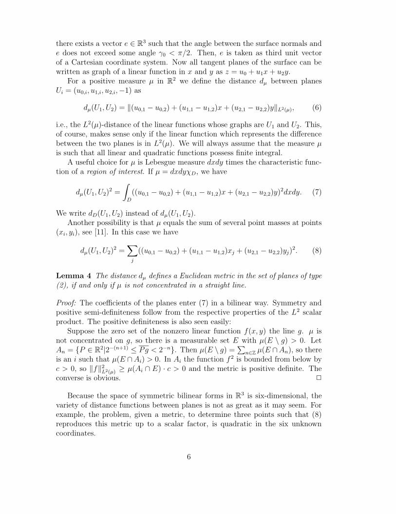
Figure 1: Approximation of a set of planes by a developable surface

A good choice for µi would be wiχDidxdy. An example of this can be seen in

Fig. 1. The positive weights wi can be used to assign more or less importanceto the single parameter values vi. It would also be possible to choose different

7

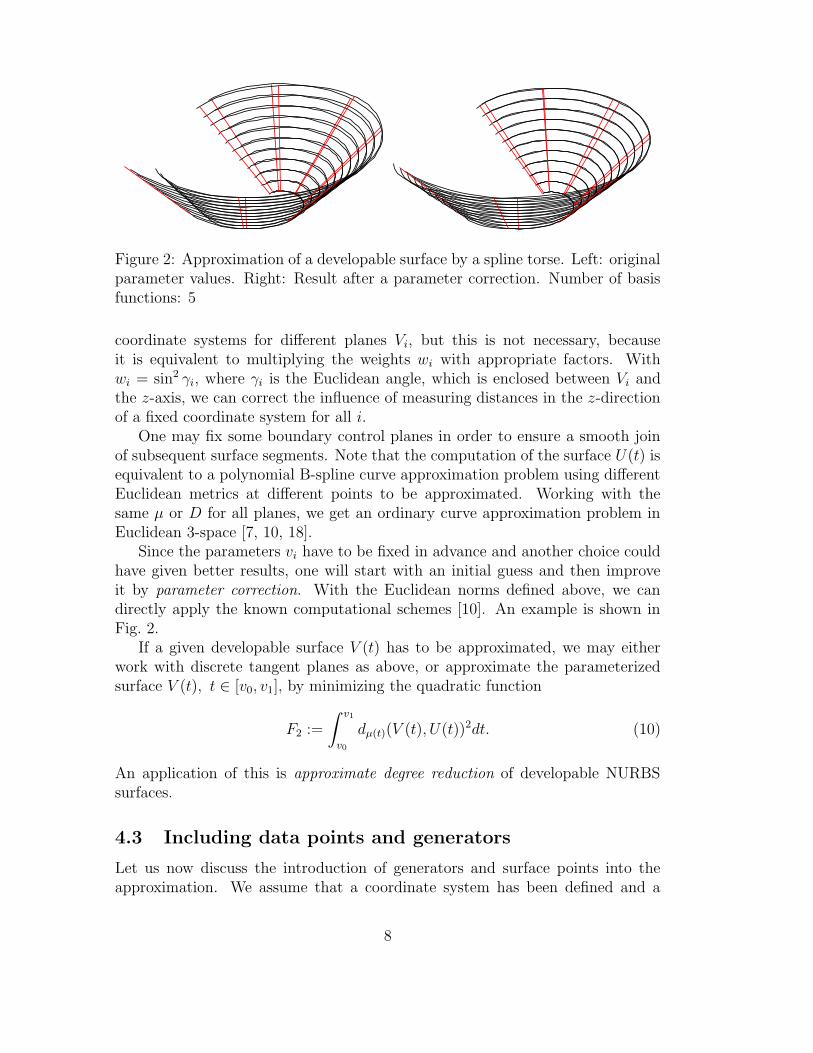
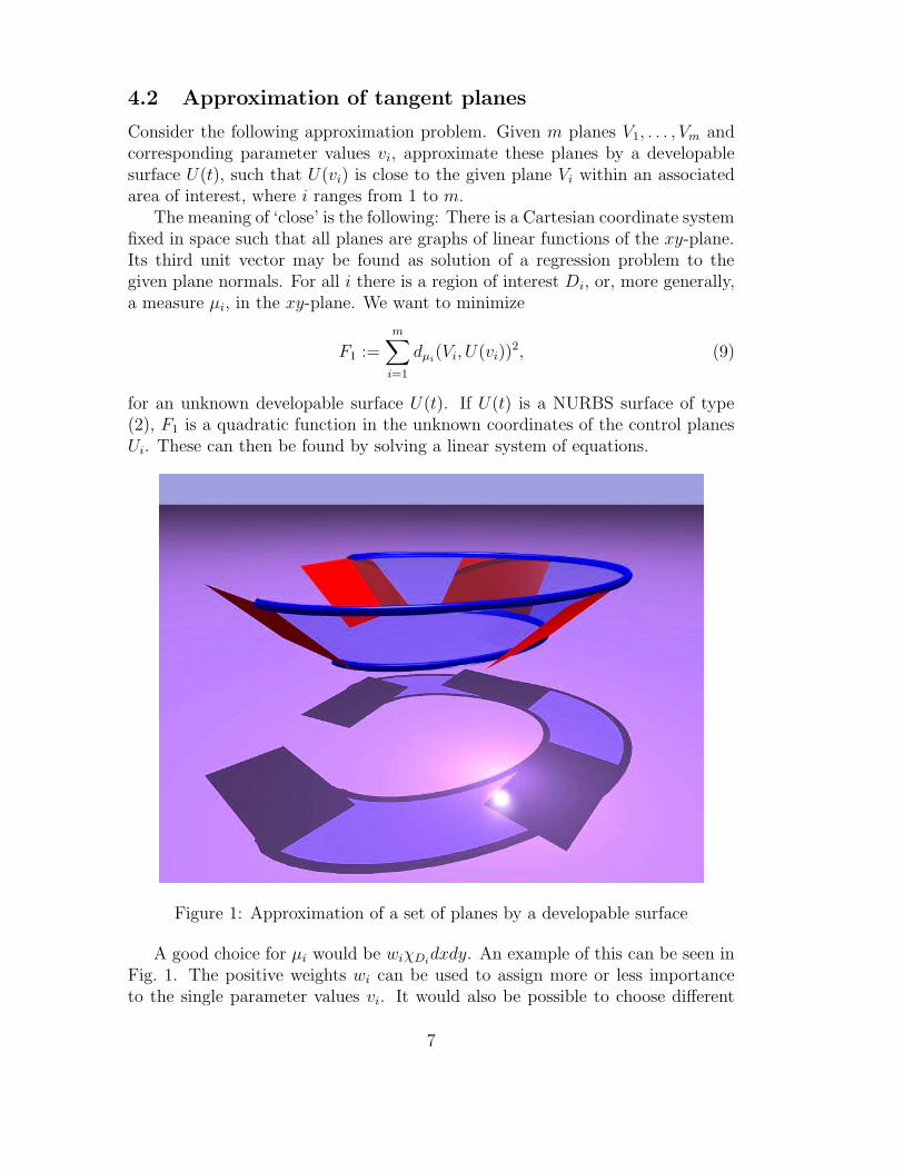
Figure 2: Approximation of a developable surface by a spline torse. Left: originalparameter values. Right: Result after a parameter correction. Number of basisfunctions: 5

coordinate systems for different planes Vi, but this is not necessary, becauseit is equivalent to multiplying the weights wi with appropriate factors. Withwi = sin2 γi, where γi is the Euclidean angle, which is enclosed between Vi andthe z-axis, we can correct the influence of measuring distances in the z-directionof a fixed coordinate system for all i.

One may fix some boundary control planes in order to ensure a smooth joinof subsequent surface segments. Note that the computation of the surface U(t) isequivalent to a polynomial B-spline curve approximation problem using differentEuclidean metrics at different points to be approximated. Working with thesame µ or D for all planes, we get an ordinary curve approximation problem inEuclidean 3-space [7, 10, 18].

Since the parameters vi have to be fixed in advance and another choice couldhave given better results, one will start with an initial guess and then improveit by parameter correction. With the Euclidean norms defined above, we candirectly apply the known computational schemes [10]. An example is shown inFig. 2.

If a given developable surface V (t) has to be approximated, we may eitherwork with discrete tangent planes as above, or approximate the parameterizedsurface V (t), t ∈ [v0, v1], by minimizing the quadratic function

F2 :=

∫ v1

v0

dµ(t)(V (t), U(t))2dt. (10)

An application of this is approximate degree reduction of developable NURBSsurfaces.

4.3 Including data points and generators

Let us now discuss the introduction of generators and surface points into theapproximation. We assume that a coordinate system has been defined and a

8

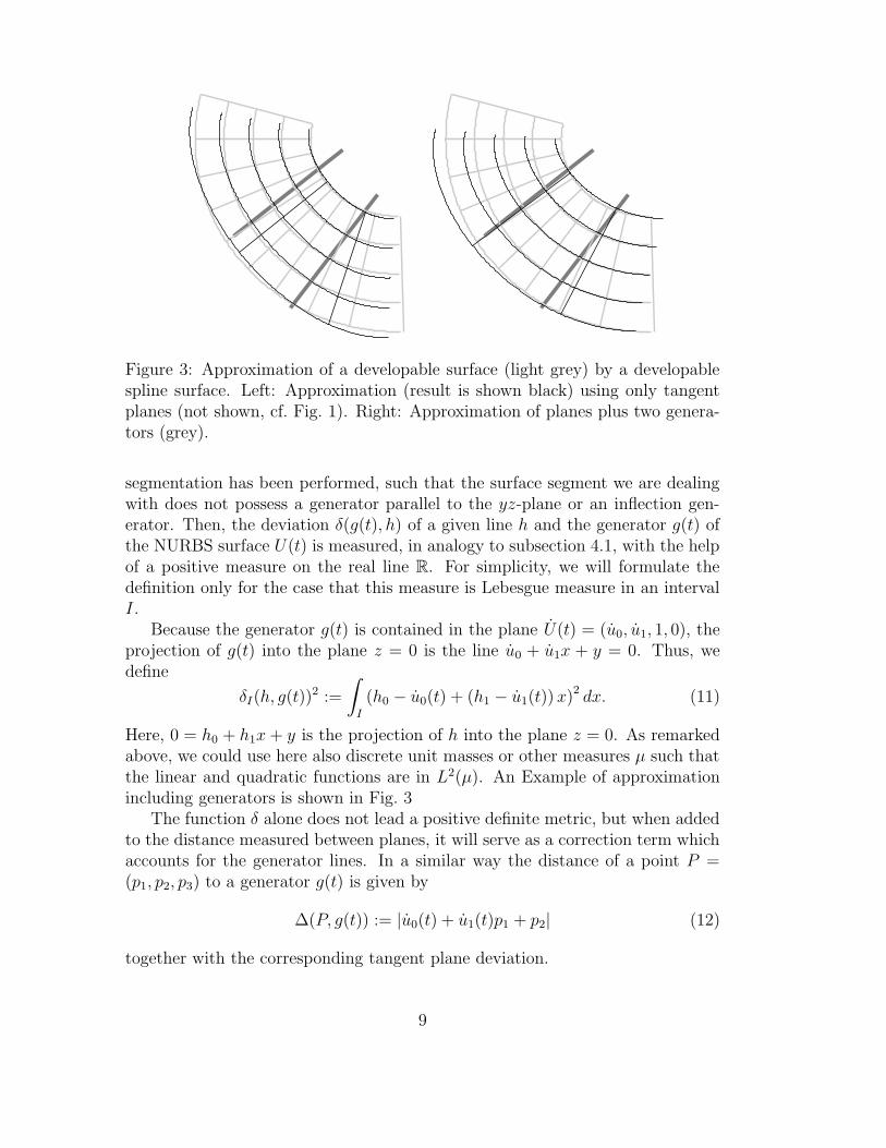
Figure 3: Approximation of a developable surface (light grey) by a developablespline surface. Left: Approximation (result is shown black) using only tangentplanes (not shown, cf. Fig. 1). Right: Approximation of planes plus two genera-tors (grey).

segmentation has been performed, such that the surface segment we are dealingwith does not possess a generator parallel to the yz-plane or an inflection gen-erator. Then, the deviation δ(g(t), h) of a given line h and the generator g(t) ofthe NURBS surface U(t) is measured, in analogy to subsection 4.1, with the helpof a positive measure on the real line R. For simplicity, we will formulate thedefinition only for the case that this measure is Lebesgue measure in an intervalI.

Because the generator g(t) is contained in the plane U(t) = (u0, u1, 1, 0), theprojection of g(t) into the plane z = 0 is the line u0 + u1x + y = 0. Thus, wedefine

δI(h, g(t))2 :=

∫

I

(h0 − u0(t) + (h1 − u1(t)) x)2 dx. (11)

Here, 0 = h0 + h1x + y is the projection of h into the plane z = 0. As remarkedabove, we could use here also discrete unit masses or other measures µ such thatthe linear and quadratic functions are in L2(µ). An Example of approximationincluding generators is shown in Fig. 3

The function δ alone does not lead a positive definite metric, but when addedto the distance measured between planes, it will serve as a correction term whichaccounts for the generator lines. In a similar way the distance of a point P =(p1, p2, p3) to a generator g(t) is given by

∆(P, g(t)) := |u0(t) + u1(t)p1 + p2| (12)

together with the corresponding tangent plane deviation.

9

Given m tangent planes Vi plus generators gi, we can approximate these databy a NURBS surface of the form (3) as follows. After an appropriate segmen-tation (see the discussion above) and the choice of local coordinate systems, theplane coordinates Vi = (. . . , vi,−1) with vi 6= vj if i 6= j, already determinethe parameters vi which have to be used in formulas like (9). Then, with themeasures µi from (9) and intervals Ii from (11), we define the quadratic function

F3 :=m∑

i=1

(dµi

(Vi, U(vi))2 + αiδIi

(gi, g(vi))2). (13)

Again, weights αi can be used to correct error measurement directions or givemore importance to certain indices i. The surface U(t) then is found as the linearcombination of the basis functions which minimizes F3.

Analogously, we can incorporate data points into the approximation. If datapoints or generators are given without tangent planes, the latter must be esti-mated before this method can be applied. There is no problem in setting up thecounterpart to (10) for the approximation of a given developable surface.

4.4 Controlling the curve of regression

Since its line of regression is a singularity of a developable surface, it is desirablethat it should lie outside some pre-defined area of interest. To achieve this whenapproximating tangent planes and generators like in the previous subsection, wecan do the following:

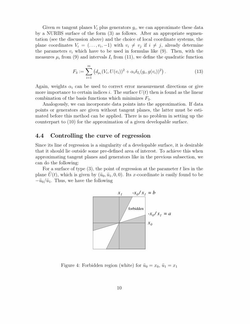
For a surface of type (3), the point of regression at the parameter t lies in theplane U(t), which is given by (u0, u1, 0, 0). Its x-coordinate is easily found to be−u0/u1. Thus, we have the following

x 0

x 1

forbidden

-x / x = b 0 1

-x / x = a 0 1

Figure 4: Forbidden region (white) for u0 = x0, u1 = x1

10

Lemma 5 In order to keep the point of regression outside the area a ≤ x ≤ b,the surface U(t) of type (3) must satisfy −u0/u1 6∈ [a, b], or, equivalently,

∣∣∣∣u0(t)

u1(t)+ c

∣∣∣∣ > r, (14)

with c = (b + a)/2 and r = (b − a)/2.

The forbidden area can be seen in Fig. 4.If the spline space which contains the functions u0(t) and u1(t) has the prop-

erty that the second derivatives of its members are contained in the spline spacewhich enjoys the two-dimensional convex hull property, it is easy to formulate acondition on the control points of the curve (u0, u1):

Lemma 6 In the situation mentioned above, if all control points of the curve(u0(t), u1(t)), are situated in one of the two connected components of the greyarea indicated in Fig. 4, then the line of regression is outside the area a ≤ x ≤ b.

Proof: This follows immediately from the convex hull property of the spline space,because then the curve (u0, u1) is entirely contained in one of the two grey regionsabove. 2

Note that ‘outside the area a ≤ x ≤ b’ does not mean ‘on one of the two sidesof the area a ≤ x ≤ b’. The curve of regression can have points at infinity andchange from one side to the other. The two regions in Fig. 4 do not correspondto the two sides of the region a ≤ x ≤ b.

We should also remark that we tacitly also excluded the case (u0, u1) = (0, 0)as ‘forbidden’, because the corresponding point of regression is a point at infinitywhich is contained in the projective extension of all regions of the form a ≤ x ≤ b.This however does not matter very much because it does not occur in the genericcase anyway, and if it does, we could apply a coordinate transformation.

It is well known that the second derivatives of B-spline functions are B-splinefunctions of a lower degree, so the lemma is applicable in this case.

Example: If ui(t) are B-spline functions of order two, their second derivatives arepiecewise constant and it is very easy to test whether or not the line of regressionmeets the region a ≤ x ≤ b.

Example: If ui(t) are B-spline functions of order three, their second derivativesare piecewise linear and lemma 6 is sharp, which means, that the line of regressionavoids the region a ≤ x ≤ b if and only if the control points of the curve (u0, u1)are contained in one of the two convex regions of Fig. 4.

We are going to describe an algorithm how to find the developable surfacecontained in a given spline space which is closest to a given developable surfacein some sense which was previously defined.

11

Choose one of the two grey convex unbounded polytopes of Fig. 4 and callit K. The spline space which contains u0 and u1 shall have basis functionsf1, . . . , fn. The second derivatives f0, . . . , fn are contained in a spline space withbasis functions g1, . . . , gm and can therefore be written as

fi(t) =∑

j

rijgj(t).

The rij are either well known or can be found numerically by differentiating thefi twice and then approximating this function by a linear combination of the gj .

Thus there is a linear mapping L which maps the sequence of control points ofthe curve (u0(t), u1(t)) to the sequence of control points of (u0(t), u1(t)). Now thesequence of control points of the second derivative curve is contained in K×. . .×Kif and only if the sequence of control points of the curve (u0, u1) is contained inthe convex polytope

K = L−1(K × . . . × K).

The equations of K are very simple, therefore so are the equations of the m-foldproduct of K with itself. The equations of its L-preimage are easily found bysolving a linear system.

Now we are able to reformulate the problem as follows: Given a convex poly-hedron K in R

r together with a scalar product and a point o. Find the pointp ∈ K which is closest to o in the sense of the metric which is defined by thescalar product. This problem is well known and there is an extensive literatureabout it.

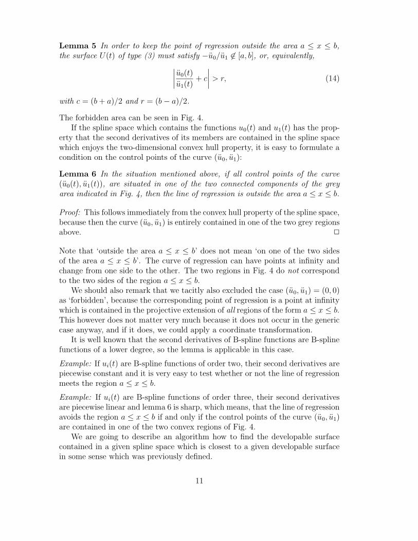
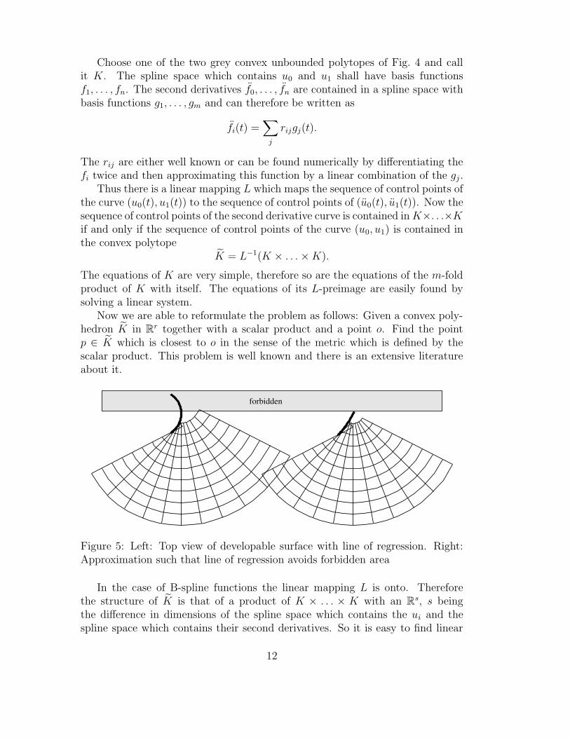
forbidden

Figure 5: Left: Top view of developable surface with line of regression. Right:Approximation such that line of regression avoids forbidden area

In the case of B-spline functions the linear mapping L is onto. Thereforethe structure of K is that of a product of K × . . . × K with an R

s, s beingthe difference in dimensions of the spline space which contains the ui and thespline space which contains their second derivatives. So it is easy to find linear

12

x

y

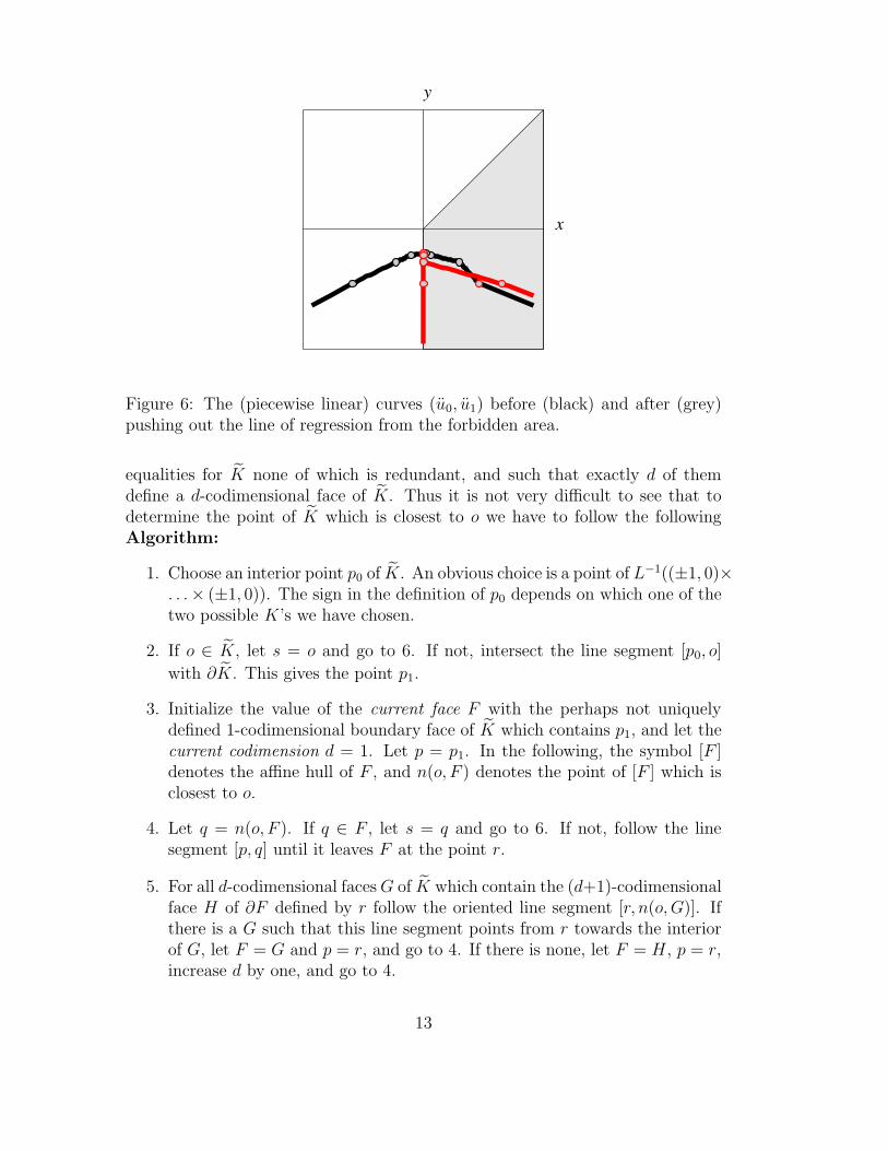
Figure 6: The (piecewise linear) curves (u0, u1) before (black) and after (grey)pushing out the line of regression from the forbidden area.

equalities for K none of which is redundant, and such that exactly d of themdefine a d-codimensional face of K. Thus it is not very difficult to see that todetermine the point of K which is closest to o we have to follow the followingAlgorithm:

1. Choose an interior point p0 of K. An obvious choice is a point of L−1((±1, 0)×. . .× (±1, 0)). The sign in the definition of p0 depends on which one of thetwo possible K’s we have chosen.

2. If o ∈ K, let s = o and go to 6. If not, intersect the line segment [p0, o]

with ∂K. This gives the point p1.

3. Initialize the value of the current face F with the perhaps not uniquelydefined 1-codimensional boundary face of K which contains p1, and let thecurrent codimension d = 1. Let p = p1. In the following, the symbol [F ]denotes the affine hull of F , and n(o, F ) denotes the point of [F ] which isclosest to o.

4. Let q = n(o, F ). If q ∈ F , let s = q and go to 6. If not, follow the linesegment [p, q] until it leaves F at the point r.

5. For all d-codimensional faces G of K which contain the (d+1)-codimensionalface H of ∂F defined by r follow the oriented line segment [r, n(o,G)]. Ifthere is a G such that this line segment points from r towards the interiorof G, let F = G and p = r, and go to 4. If there is none, let F = H, p = r,increase d by one, and go to 4.

13

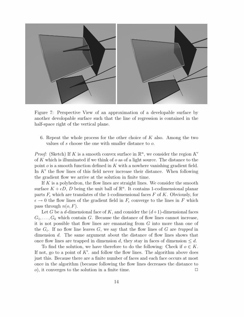
Figure 7: Perspective View of an approximation of a developable surface byanother devolopable surface such that the line of regression is contained in thehalf-space right of the vertical plane.

6. Repeat the whole process for the other choice of K also. Among the twovalues of s choose the one with smaller distance to o.

Proof: (Sketch) If K is a smooth convex surface in Rn, we consider the region K ′

of K which is illuminated if we think of o as of a light source. The distance to thepoint o is a smooth function defined in K with a nowhere vanishing gradient field.In K ′ the flow lines of this field never increase their distance. When followingthe gradient flow we arrive at the solution in finite time.

If K is a polyhedron, the flow lines are straight lines. We consider the smoothsurface K + εD, D being the unit ball of R

n. It contains 1-codimensional planarparts Fε which are translates of the 1-codimensional faces F of K. Obviously, forε → 0 the flow lines of the gradient field in Fε converge to the lines in F whichpass through n(o, F ).

Let G be a d-dimensional face of K, and consider the (d+1)-dimensional facesG1, . . . , Gk which contain G. Because the distance of flow lines cannot increase,it is not possible that flow lines are emanating from G into more than one ofthe Gi. If no flow line leaves G, we say that the flow lines of G are trapped indimension d. The same argument about the distance of flow lines shows thatonce flow lines are trapped in dimension d, they stay in faces of dimension ≤ d.

To find the solution, we have therefore to do the following: Check if o ∈ K.If not, go to a point of K ′. and follow the flow lines. The algorithm above doesjust this. Because there are a finite number of faces and each face occurs at mostonce in the algorithm (because following the flow lines decreases the distance too), it converges to the solution in a finite time. 2

14

Figures 5, 6 and 7 show examples. Of course other standard methods of con-vex programming can be employed also, for instance a barrier-generated path-following method. Such a method is more recommended when the structure ofthe polyhedron is not completely known [17]. We chose this algorithm, and we de-scribed it at length despited the fact that many algorithms for quadratic/convexoptimatization problems can be found in the literature, because our polyhedronhas such a simple structure that the most simple and obvious geometric algorithm,i.e., following the gradient lines on the polyhedron, does not lead to numericaldifficulties.

4.5 Approximation via multiresolution analysis

There are several ways to apply the concept of multiresolution analysis to devel-opable surfaces. One is, of course, to treat the surface of type (2) or type (3)as a curve in affine R

3 or R2, respectively. This is nothing but multiresolution

analysis for curves, and leads likewise to efficient filter bank decomposition andstorage of developable surfaces.

A different problem is the following. Just like a planar curve can be approxi-mated by an arc spline, i.e., a curve which consists of circular arcs, we may askfor an approximation of a developable surface by a surface consisting of certainquadratic cones. We could use cones of revolution, or we could use cones all ofwhose intersection curves with horizontal planes are circles. The latter will turnout to lead to the planar arc spline approximation problem.

In [25] the support functions of (locally) convex curves have been approxi-mated by trigonometric spline functions and analyzed by a generalized multires-olution analysis which was introduced in [15]. Here we are interested only in thepart of the developable surface which lies between two parallel planes. Withoutloss of generality we assume that these planes are z = 0 and z = 1. Then thesurface has intersection curves c0 and c1 with these two planes. When we approx-imate both c0 and c1 by arc splines, the unique developable surface determinedby the arc splines will be an approximant to the original surface. In order todiminish the number of lines of curvature disconinuity in the approximant evenfurther, we choose the same spline space for approximation of c0 and c1. Anexample can be seen in Fig. 9.

To accomplish this, we have to define a distance between two such surfaces.First we define a distance between planes whose contour lines are parallel. It willbe a positive definite quadratic form of the oriented distances h0 and h1 of thecontour lines in z = 0 and z = 1, respectively. One obvious possibility is

q(h0, h1) = h20 + h2

1. (15)

Another one is

q(h0, h1) =

∫ 1

0

h(z)2dz =1

3(h2

0 + h0h1 + h21), (16)

15

z=0

z=1

h > 0 0

h < 0 1

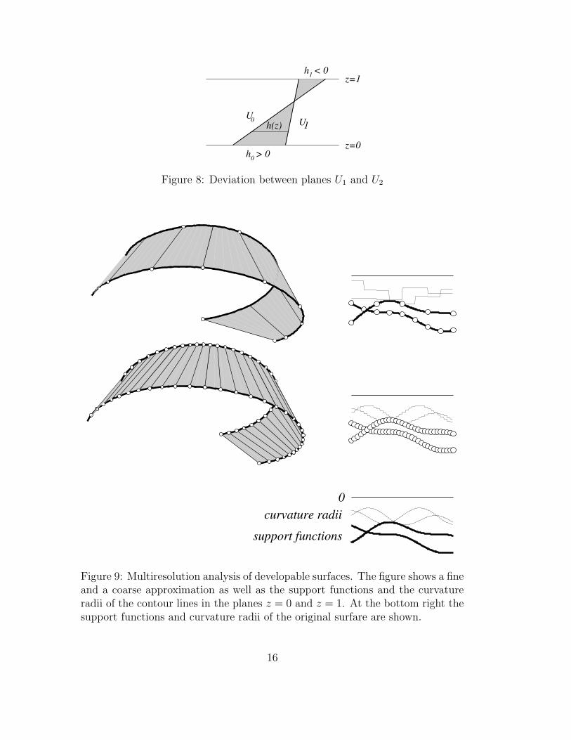
U 0 U 1h(z)

Figure 8: Deviation between planes U1 and U2

0curvature radii

support functions

Figure 9: Multiresolution analysis of developable surfaces. The figure shows a fineand a coarse approximation as well as the support functions and the curvatureradii of the contour lines in the planes z = 0 and z = 1. At the bottom right thesupport functions and curvature radii of the original surfare are shown.

16

where h(z) = zh1 + (1 − z)h0.Now suppose that fi(ϕ) and gi(ϕ) are the support functions of the intersection

curves of two developable surfaces Φ and Ψ with planes z = i, i = 0, 1. For givenϕ, the distance between the tangent planes to Φ and Ψ which belong to the angleϕ, can be expressed in terms of h0(ϕ) = f0(ϕ)−g0(ϕ) and h1(ϕ) = f1(ϕ)−g1(ϕ).Thus we define

dµ(Φ, Ψ) =

∫q(f0(ϕ) − g0(ϕ), f1(ϕ) − g1(ϕ))dµ(ϕ), (17)

with an appropriate positive measure µ. Typically this will be Lebesgue measurein an interval. We further let

β((u0, u1), (v0, v1)) =1

2(q(u0 + v0, u1 + v1) − q(u0, u1) − q(v0, v1)), (18)

which is the unique symmetric bilinear form whose restriction to the diagonalgives q. Then the distance (17) is induced by the following scalar product onL2(µ) ⊕ L2(µ):

ιµ((f0, f1), (g0, g1)) =

∫β((f0(ϕ), f1(ϕ)), (g0(ϕ), g1(ϕ)))dµ(ϕ) (19)

Lemma 7 The scalar product (19) is positive definite in L2(µ) ⊕ L2(µ).

Proof: Clearly∫

q(f0, f1)dµ(ϕ) = 0 implies q(f0, f1) = 0 almost everywhere (a.e.),so f0 = 0 a.e. and f1 = 0 a.e., by positive definiteness of β. 2

Suppose we already have a generalized multiresolution analysis in L2(µ), givenby the sequence

V0 ⊆ V1 ⊆ . . .

Vi+1 = Vi ⊕ Wi and Wi ⊥ Vi

L2(µ) =⋃

Vi = V0 ⊕ W0 ⊕ W1 ⊕ . . .

(20)

Then we have the following

Theorem 8 The scalar product (19) is compatible with the direct sum topologyof L2(µ) ⊕ L2(µ). If we let

Vi = Vi ⊕ Vi ⊂ L2(µ) ⊕ L2(µ) and Wi = Wi ⊕ Wi, (21)

then the following is a generalized multiresolution analysis:

V0 ⊆ V1 ⊆ . . .

Vi+1 = Vi ⊕ Wi and Wi ⊥ι Vi

L2(µ) ⊕ L2(µ) =⋃

Vi = V0 ⊕ W0 ⊕ W1 ⊕ . . .

(22)

17

Proof: Clearly⋃

Vi is dense in L2(µ) ⊕ L2(µ) because⋃

Vi is dense in L2(µ).Let (aij) be the coordinate (2 × 2)-matrix of β. If f0, f1 ∈ Wi and g0, g1 ∈ Vi,then ι((f0, f1), (g0, g1)) =

∫ ∑aijfi(ϕ)gj(ϕ)dµ(ϕ) = 0 because Vi ⊥ Wi. This

implies Vi ⊥ι Wi and the orthogonal direct sum decomposition L2(µ) ⊕ L2(µ) =

V0 ⊕ W0 ⊕ Wi . . .Let πi denote the orthogonal projection L2(µ) → Vi and πi denote the ortho-

gonal projection onto Vi. It is now clear that πi(f0, f1) = (πi(f0), πi(f1)). Wehave (f0n, f1n) → (f0, f1) ⇐⇒ f0n → f0 and f1n → f1, so the topology definedby ι coincides with the topology of the direct sum. 2

Corollary 9 Approximation of a developable surface in the sense that the supportfunctions of both contour lines are chosen from the spline space Vi of trigonometricspline functions such that (17) is minimal, is done by approximating each of thesupport functions of the contour lines separately in the sense of L2(µ).

Proof: The proof of the previous theorem shows that the ι-orthogonal projectionπi onto Vi coincides with (πi, πi), where πi is the orthogonal projection onto Vi.2

Acknowledgements

This work has been supported in part by grant No. P12252-MAT of the AustrianScience Foundation. The approximation and multiresolution algorithms havebeen implemented by M. Pfeifer and N. Pomaroli.

References

[1] G. Aumann, G., Interpolation with developable Bezier patches, Comput.Aided Geom. Design 8 (1991) , 409–420.

[2] G. Aumann, A closer look at developable Bezier surfaces, J. of TheoreticalGraphics and Computing 7 (1994) , 12–26.

[3] R.M.C. Bodduluri, B. Ravani, Geometric design and fabrication of devel-opable surfaces, ASME Adv. Design Autom. 2 (1992) , 243–250.

[4] R.M.C. Bodduluri, R.M.C., B. Ravani, Design of developable surfaces usingduality between plane and point geometries, Computer-Aided Design 25

(1993) , 621–632.

[5] J. Chalfant, T. Maekawa, Design for manufacturing using B-spline devel-opable surfaces, preprint, MIT 1997.

18

[6] J. Chalfant, T. Maekawa, Computation of inflection lines and geodesics ondevelopable surfaces, preprint, MIT 1997.

[7] G. Farin, Curves and Surfaces for Computer Aided Geometric design, Aca-demic Press, Boston 1992.

[8] W.H. Frey, D. Bindschadler, Computer aided design of a class of developableBezier surfaces, General Motors R&D Publication 8057 (1993) .

[9] J. Hoschek, Dual Bezier curves and surfaces, in: Surfaces in Computer AidedGeometric Design, R.E. Barnhill and W. Boehm, eds., North Holland, 1983,pp. 147–156.

[10] J. Hoschek, D. Lasser, Fundamentals of Computer Aided Geometric Design,A. K. Peters, Wellesley, Mass. 1993.

[11] J. Hoschek, H. Pottmann, Interpolation and approximation with developableB–spline surfaces, in Mathematical Methods for Curves and Surfaces, M.Dæhlen, T. Lyche and L.L. Schumaker, eds., Vanderbilt University Press,Nashville 1995, pp. 255–264.

[12] J. Hoschek, M. Schneider, Interpolation and approximation with devel-opable surfaces, in: Curves and Surfaces with Applications in CAGD, A. LeMehaute, C. Rabut and L.L. Schumaker, eds., Vanderbilt University Press,Nashville 1997, pp. 185–202.

[13] J. Hoschek, U. Schwanecke, Interpolationand approximation with ruled sur-faces, in: The Mathematics of Surfaces VIII, R. Cripps Ed., InformationGeometers, 1998, pp. 213–231.

[14] J. Lang, O. Roschel, Developable (1, n)-Bezier surfaces, Comput. AidedGeom. Design 9 (1992) , 291–298.

[15] T. Lyche, L.L. Schumaker, L-Spline Wavelets, in: Wavelets: Theory, Algo-rithms, and Applications C. Chui, L. Montefusco and L. Puccio Eds., Aca-demic Press, 1994, pp. 197–212.

[16] M. Neamtu, H. Pottmann, L.L. Schumaker, Dual focal splines and ratio-nal curves with rational offsets, Mathematical Engineering in Industry, toappear.

[17] Yu. Nesterov, A. Nemirovskii, Interior-Point Polynomial Algorithms in Con-vex Programming, SIAM, 1994.

[18] L. Piegl, W. Tiller, The NURBS book, Springer, 1995.

19

[19] H. Pottmann, Studying NURBS curves and surfaces with classical geometry,in Mathematical Methods for Curves and Surfaces, M. Dæhlen, T. Lyche andL. L. Schumaker, eds., Vanderbilt University Press, Nashville 1995, pp. 413–438.

[20] H. Pottmann, G. Farin, Developable rational Bezier and B–spline surfaces,Comput. Aided Geom. Design 12 (1995) , 513–531.

[21] T. Randrup, Approximation by cylinder surfaces. Technical Report No. 41,Institut fur Geometrie, Vienna University of Technology 1997.

[22] M. Schneider, Approximation von Blechhalterflachen mit Torsen in B–SplineDarstellung, Diplomarbeit, TH Darmstadt 1996.

[23] E. Stollnitz, T. DeRose, H. Salesin, Wavelets for Computer Graphics, Mor-gan Kaufmann Publishers, San Francisco 1996

[24] R. Vatter, Approximation von Datenpunkten mit Torsen in B–SplineDarstellung, Diplomarbeit, TH Darmstadt 1996.

[25] J. Wallner, Generalized multiresolution analysis for arc splines, in: Math-ematical Methods for Curves and Surfaces II, M. Dæhlen, T. Lyche, L. L.Schumaker (eds.), Nashville University Press, 1998. pp. 537–544

20