1 Improved Approximation Algorithms for Matroid and ...cswamy/papers/mmed-journ.pdf · Improved Approximation Algorithms for Matroid and Knapsack ... Improved Approximation Algorithms

1

Improved Approximation Algorithms for Matroid and KnapsackMedian Problems and Applications

CHAITANYA SWAMY, University of Waterloo

We consider the matroid median problem [Krishnaswamy et al. 2011], wherein we are given a set of facilitieswith opening costs and a matroid on the facility-set, and clients with demands and connection costs, and weseek to open an independent set of facilities and assign clients to open facilities so as to minimize thesum of the facility-opening and client-connection costs. We give a simple 8-approximation algorithm for thisproblem based on LP-rounding, which improves upon the 16-approximation in [Krishnaswamy et al. 2011].We illustrate the power and versatility of our techniques by deriving: (a) an 8-approximation for the two-matroid median problem, a generalization of matroid median that we introduce involving two matroids;and (b) a 24-approximation algorithm for matroid median with penalties, which is a vast improvementover the 360-approximation obtained in [Krishnaswamy et al. 2011]. We show that a variety of seeminglydisparate facility-location problems considered in the literature—data placement problem, mobile facilitylocation, k-median forest, metric uniform minimum-latency UFL—in fact reduce to the matroid median ortwo-matroid median problems, and thus obtain improved approximation guarantees for all these problems.Our techniques also yield an improvement for the knapsack median problem.

Categories and Subject Descriptors: F.2.2 [Analysis of Algorithms and Problem Complexity]: Non-numerical Algorithms and Problems—computations on discrete structures; G.2 [Discrete Mathematics]:Miscellaneous; G.1.6 [Numerical Analysis]: Optimization

General Terms: Algorithms, Theory

Additional Key Words and Phrases: Approximation algorithms, Linear programming and LP rounding, Fa-cility location k-median and matroid median, Submodular and matroid polyhedra, Knapsack constraints

ACM Reference Format:Chaitanya Swamy. 2016. Improved Approximation Algorithms for Matroid and Knapsack Median Problemsand Applications. ACM Trans. Algor. V, N, Article 1 (January 2016), 23 pages.DOI: http://dx.doi.org/10.1145/2790133

1. INTRODUCTIONWe investigate facility location problems wherein the set of open facilities have to sat-isfy some matroid independence constraints or knapsack constraints. Specifically, weconsider the matroid median problem, which is defined as follows. As in the uncapaci-tated facility location problem, we are given a set of facilities F and a set of clients D.Each facility i has an opening cost of fi. Each client j ∈ D has demand dj and assigningclient j to facility i incurs an assignment cost of djcij proportional to the distance be-tween i and j. Further, we are given a matroid M = (F , I) on the set of facilities. Thegoal is to choose a set F ∈ I of facilities to open that forms an independent set in M ,and assign each client j to a facility i(j) ∈ F so as to minimize the total facility-opening

A preliminary version [Swamy 2014] appeared in the Proceedings of the 17th APPROX, 2014.Research supported in part by NSERC grant 327620-09, an NSERC Discovery Accelerator SupplementAward, and an Ontario Early Researcher Award. Author’s address: Chaitanya Swamy, Dept. of Combina-torics & Optimization, University of Waterloo, 200 University Avenue West, Waterloo, ON N2L 3G1, Canada.Email: [email protected] to make digital or hard copies of all or part of this work for personal or classroom use is grantedwithout fee provided that copies are not made or distributed for profit or commercial advantage and thatcopies bear this notice and the full citation on the first page. Copyrights for components of this work ownedby others than the author(s) must be honored. Abstracting with credit is permitted. To copy otherwise, orrepublish, to post on servers or to redistribute to lists, requires prior specific permission and/or a fee. Requestpermissions from [email protected]© 2016 Copyright held by the owner/author(s). Publication rights licensed to ACM. 1549-6325/2016/01-

ART1 $15.00DOI: http://dx.doi.org/10.1145/2790133

ACM Transactions on Algorithms, Vol. V, No. N, Article 1, Publication date: January 2016.

1:2 C. Swamy

and client-assignment costs, that is,∑i∈F fi +

∑j∈D djci(j)j . We assume that the fa-

cilities and clients are located in a common metric space, so the distances cij form ametric.

The matroid median problem is a generalization of the metric k-median problem,which is the special case where M is a uniform matroid (and there are no facility-opening costs), and is thus, NP-hard. The matroid median problem without facility-opening costs was introduced recently by Krishnaswamy et al. [Krishnaswamy et al.2011], who gave a 16-approximation algorithm for this problem.

Our contributions are threefold.• We devise an improved 8-approximation algorithm for the matroid-median problem

(Section 3). Moreover, notably, our algorithm is significantly simpler and cleanerthan the one in [Krishnaswamy et al. 2011], and satisfies the stronger propertythat it is a Lagrangian-multiplier-preserving 8-approximation algorithm (see Re-mark 3.9). The effectiveness and versatility of our simpler approach for matroidmedian is further highlighted when we consider some natural extensions of matroidmedian in Section 4. We leverage the techniques underlying our simpler and cleaneralgorithm for matroid median to devise: (a) an 8-approximation algorithm for thetwo-matroid median problem (Section 4.1), which is an extension that we introduceinvolving two matroids that captures some interesting facility-location problemsconsidered in the literature; and (b) a 24-approximation algorithm (Section 4.2) forthe matroid median problem with penalties, wherein we are allowed to leave clientunassigned and incur a penalty for each unassigned client; this constitutes a vastimprovement over the approximation ratio of 360 obtained by Krishnaswamy etal. [Krishnaswamy et al. 2011].• We show that the matroid median and two-matroid median problem turn out to be

rather fundamental problems by showing in Section 5 that a variety of facility loca-tion problems that have been considered in the literature can be cast as instancesof matroid median or two-matroid median. These include the data placement prob-lem [Baev and Rajaraman 2001; Baev et al. 2008], mobile facility location [Friggstadand Salavatipour 2011; Ahmadian et al. 2013], k-median forest [Gørtz and Nagara-jan 2011], and metric uniform minimum-latency UFL [Chakrabarty and Swamy2011]. This not only gives a unified framework for viewing these seemingly dis-parate problems, but also our approximation guarantee of 8 yields improved, and insome cases, the first, approximation guarantees for all these problems.• We adapt our techniques to also obtain an improvement for the knapsack median

problem [Krishnaswamy et al. 2011; Kumar 2012] (Section 6).Our improvement for matroid median comes from an improved, simpler round-

ing procedure for a natural LP relaxation of the problem also considered in [Krish-naswamy et al. 2011]. We show that a clustering step introduced in [Charikar et al.2002] for the k-median problem coupled with two applications of the integrality of theintersection of two submodular (or matroid) polyhedra—one to obtain a half-integralsolution, and another to obtain an integral solution—suffices to obtain the desired ap-proximation ratio. In contrast, the algorithm in [Krishnaswamy et al. 2011] starts offwith the clustering step in [Charikar et al. 2002], but then further dovetails the round-ing procedure of [Charikar et al. 2002] creating trees, then stars, and then applies theintegrality of the intersection of two submodular polyhedra.

There is great deal of similarity between the the rounding algorithm of [Krish-naswamy et al. 2011] for matroid median and the rounding algorithm of Baev andRajaraman [Baev and Rajaraman 2001] for the data placement problem, who also per-form the initial clustering step in [Charikar et al. 2002] and then create trees and then


Improved Approximation Algorithms for Matroid and Knapsack Median Problems 1:3

stars and use these to obtain an integral solution. In contrast, our simpler, improvedrounding algorithm is similar to the rounding algorithm in [Baev et al. 2008] for dataplacement, who use the initial clustering step of [Charikar et al. 2002] coupled withtwo min-cost flow computations—one to obtain a half-integral solution and anotherto obtain an integral solution—to obtain the final solution. These similarities are notsurprising since, as mentioned above, we show in Section 5 that the data-placementproblem is a special case of the matroid median problem. In fact, our improvementsare analogous to those obtained for the data-placement problem by Baev, Rajaraman,and Swamy [Baev et al. 2008] over the guarantees in [Baev and Rajaraman 2001], andstem from similar insights.

A common theme to emerge from our work and [Baev et al. 2008] is that in varioussettings, the initial clustering step introduced by [Charikar et al. 2002] imparts suffi-cient structure to the fractional solution so that one can then round it using two appli-cations of suitable integrality-results from combinatorial optimization. First, this ini-tial clustering can be used to derive a half-integral solution. This was observed explic-itly in [Baev and Rajaraman 2001] and is implicit in [Krishnaswamy et al. 2011], andmaking this explicit yields significant dividends. Second, and this is the oft-overlookedinsight (in [Baev and Rajaraman 2001; Krishnaswamy et al. 2011]), a half-integral so-lution can be easily rounded, and in a better way, without resorting to creating treesand then stars etc. as in the algorithm of [Charikar et al. 2002]. This is due to thefact that a half-integral solution is already “filtered”: if client j is assigned to facilityi fractionally, then one can bound cij in terms of the assignment cost paid by the frac-tional solution for j (see Section 3). This enables one to use a standard facility-locationclustering step to set up a suitable combinatorial-optimization problem possessing anintegrality property, and hence, round the half-integral solution. The resulting algo-rithm is typically both simpler and has a better approximation ratio than what onewould obtain by mimicking the steps of [Charikar et al. 2002] involving creating trees,stars etc.

Recently, Charikar and Li [Charikar and Li 2012] obtained a 9-approximation al-gorithm for the matroid-median problem; our results were obtained independently.1While there is some similarity between our ideas and those in [Charikar and Li 2012],we feel that our algorithm and analysis provides a more illuminating explanation ofwhy matroid median and some of its extensions (e.g., two-matroid median, matroid me-dian with penalties; see Section 4) are “easy” to approximate, whereas other variantssuch as matroid-intersection median (Section 4) are inapproximable. It remains to beseen if our ideas coupled with the dependent-rounding procedure used in [Charikarand Li 2012] for the k-median problem leads to further improvements for the matroidmedian problem; we leave this as future work.

2. AN LP RELAXATION FOR MATROID MEDIANWe can express the matroid median problem as an integer program and relax theintegrality constraints to get a linear program (LP). Throughout we use i to indexfacilities in F , and j to index clients in D. Let r denote the rank function of the matroidM = (F , I).

1A manuscript containing the 8-approximation for matroid median was circulated privately in 2012; thecurrent version was posted on the arXiv in Nov. 2013.


1:4 C. Swamy

min∑i

fiyi +∑j

∑i

djcijxij (P)

s.t.∑i

xij ≥ 1 ∀j (1)∑i∈S

yi ≤ r(S) ∀S ⊆ F (2)

0 ≤ xij ≤ yi ∀i, j. (3)

Variable yi indicates if facility i is open, and xij indicates if client j is assigned tofacility i. The first and third constraints say that each client must be assigned to anopen facility. The second constraint encodes the matroid independence constraint. Aninteger solution corresponds exactly to a solution to our problem. We note that (P) canbe solved in polytime since (for example) a polytime algorithm for submodular-functionminimization yields an efficient separation oracle.

3. A SIMPLE 8-APPROXIMATION ALGORITHM VIA LP-ROUNDINGLet (x, y) denote an optimal solution to (P) and OPT be its value. We first describe asimple algorithm to round (x, y) to an integer solution losing a factor of at most 10.In Section 3.4, we use some additional insights to improve the approximation ratioto 8. We use the terms connection cost and assignment cost interchangeably. We mayassume that

∑i xij = 1 for every client j.

3.1. Overview of the algorithmWe first give a high level description of the algorithm. Suppose for a moment that theoptimal solution (x, y) satisfies the following property:

for every facility i, there is at most one client j such that xij > 0. (∗)Let Fj = {i : xij > 0}. Notice that the Fj sets are disjoint. We may assume that fori ∈ Fj , we have yi = xij , so the objective function is a linear function of only the yivariables. We can then set up the following matroid intersection problem. The firstmatroid is M restricted to

⋃j Fj . The second matroid M ′ (on the same ground set⋃

j Fj) is the partition matroid defined by the Fj sets; that is, a set is independentin M ′ if it contains at most one facility from each Fj . Notice the yi-variables yield afractional point in the intersection of the matroid polyhedron of M and the matroid-base polyhedron of M ′. Since the intersection of these two polyhedra is known to beintegral (see, e.g., [Cook et al. 1998]), this means that we can round (x, y) to an integersolution of no greater cost. Of course, the LP solution need not have property (∗) so ourgoal will be to transform (x, y) to a solution that has this property without increasingthe cost by much.

Roughly speaking we want to do the following: cluster the clients inD around certain‘centers’ (also clients) such that (a) every client k is assigned to a “nearby” cluster cen-ter j whose LP assignment cost is less than that of k, and (b) the facilities serving thecluster centers in the fractional solution (x, y) are disjoint. So, the modified instancewhere the demand of a client is moved to the center of its cluster has a fractional solu-tion, namely the solution induced by (x, y), that satisfies (∗) and has cost at most OPT .Furthermore, given a solution to the modified instance we can obtain a solution to theoriginal instance losing a small additive factor. One option is to use the decompositionmethod of Shmoys et al. [Shmoys et al. 1997] for uncapacitated facility location (UFL)that produces precisely such a clustering. The problem however is that [Shmoys et al.1997] uses filtering which involves blowing up the xij and yi values, thus violating the



matroid-rank packing constraints. Chudak and Shmoys [Chudak and Shmoys 2003]use the same clustering idea but without filtering, using the dual solution to boundthe cost. The difficulty here with this approach is that there are terms with negativecoefficients in the dual objective function that correspond to the primal matroid-rankconstraints. Although [Swamy and Shmoys 2008] showed that it is possible to over-come this difficulty in certain cases, the situation here looks more complicated and itis not clear how to use their techniques.

Instead, we use the clustering technique of Charikar et al. [Charikar et al. 2002]to cluster clients and first obtain a half-integral solution (x, y), that is, every xij , yi ∈{

0, 12 , 1}

, to the modified instance with cluster centers, losing a factor of 3. Further, anysolution here will give a solution to the original instance while increasing the cost byat most 4 ·OPT . Now we use the clustering method of [Shmoys et al. 1997] without anyfiltering, since the half-integral solution (x, y) is essentially already filtered; if client jis assigned to i and i′ in x, then cij , ci′j ≤ 2(cij xij + ci′j xi′j). This final step causes usto lose an additive factor equal to the cost of (x, y), so overall we get an approximationratio of 4+3+3 = 10. In Section 3.4, we show that by further exploiting the structure ofthe half-integral solution, we can give a better bound on the cost of the integer solutionand thus obtain an 8-approximation.

We now describe each of these steps in detail. Let Cj =∑i cijxij denote the cost

incurred by the LP solution to assign one unit of demand of client j. Given a vectorv ∈ RF and a set S ⊆ F , we use v(S) to denote

∑i∈S vi.

3.2. OBTAINING A HALF-INTEGRAL SOLUTION (x, y)

Step I: Consolidating demands around centers. We first consolidate (or cluster) thedemand of clients at certain clients, that we call cluster centers. We do not modify thefractional solution (x, y) but only modify the demands so that for some clients k, thedemand dk is “moved” to a “nearby” center j. We assume every client has non-zerodemand (we can simply get rid of zero-demand clients).

Set d′j ← 0 for every j. Consider the clients in increasing order of Cj . For each clientk encountered, if there exists a client j such that d′j > 0 and cjk ≤ 4 max(Cj , Ck) = 4Ck,set d′j ← d′j + dk, otherwise set d′k ← dk. Let D = {j ∈ D : d′j > 0}. Each client in D isa cluster center. Let OPT ′ =

∑i fiyi +

∑j∈D,i d

′jcijxij denote the cost of (x, y) for the

modified instance consisting of the cluster centers.

LEMMA 3.1. (i) If j, k ∈ D, then cjk ≥ 4 max(Cj , Ck), (ii) OPT ′ ≤ OPT , and (iii) anysolution (x′, y′) to the modified instance can be converted to a solution to the originalinstance incurring an additional cost of at most 4 ·OPT .

PROOF. Suppose k was considered after j. Then d′j > 0 at this time, otherwise d′jwould remain at 0 and j would not be in D. So if cjk < 4 max(Cj , Ck) then d′k wouldremain at 0, giving a contradiction. It is clear that if we move the demand of client kto client j, then Cj ≤ Ck and cjk ≤ 4Ck. So the assignment cost for the new instance,∑j d′jCj , only decreases and the facility-opening cost

∑i fiyi does not change, hence

OPT ′ ≤ OPT . Given a solution (x′, y′) to the modified instance, if the demand of kwas moved to j the extra cost incurred in assigning k to the same facility(ies) as in x′

is at most dkcjk ≤ 4dkCk by the triangle inequality, so the total extra cost is at most4 ·OPT .

From now on we focus on the modified instance with client set D and modified de-mands d′j . At the very end we will use the above lemma to translate an integer solutionto the modified instance to an integer solution to the original instance.


1:6 C. Swamy

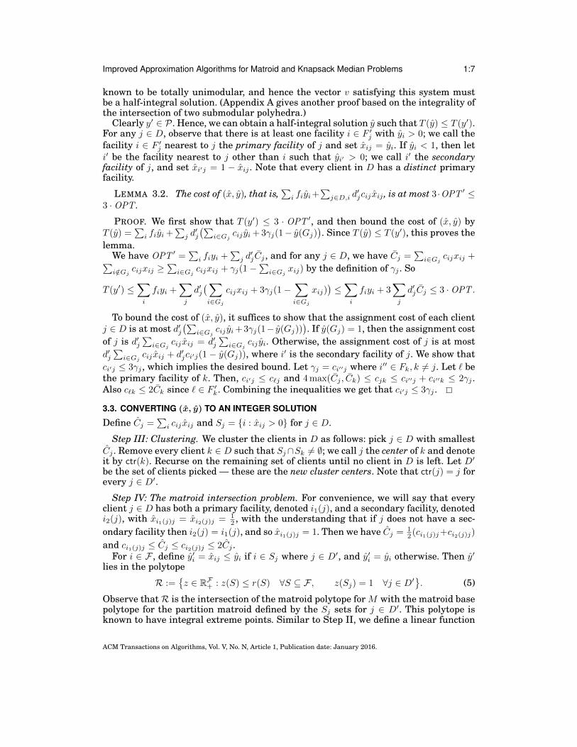
Step II: Transforming to a half-integral solution. We define the cluster of a clientj ∈ D to be the set Fj of all facilities i such that j is the center in D closest to i, thatis, Fj = {i : cij = mink∈D cik}, with ties broken arbitrarily. Let F ′j ⊆ Fj = {i ∈ Fj : cij ≤2Cj}. Define γj := mini/∈Fj cij , and let Gj = {i ∈ Fj : cij ≤ γj}; see Fig. 1. By property(i) of Lemma 3.1, we have that Fj contains all the facilities i such that cij ≤ 2Cj . Soγj ≥ 2Cj , F ′j ⊆ Gj , and

∑i∈F ′

jxij =

∑i:cij≤2Cj

xij ≥ 12 by Markov’s inequality. Clearly

the sets Fj for j ∈ D are disjoint.

Fj

F ′j

Gj

γj = cij

i

j

Fks

F ′ks

Fig. 1. Illustrating the sets Fj , F ′j , Gj , and the quantity γj . Facility i is the facility nearest to j notin Fj .

To obtain the half-integral solution, we define a suitable vector y′ that lies in a poly-tope with half-integral extreme points and construct a linear function T (.) such thatT (y′) bounds the cost of a fractional solution. We show that T (y′) ≤ 3 ·OPT ′. This im-plies that one can obtain a “better” half-integral vector y, which we then argue yieldsa half-integral solution (x, y) to the modified instance of cost at most T (y) ≤ T (y′).

To motivate the definition of T (.) and the polytope, first define y′ ∈ RF+ as follows:set y′i = xi` ≤ yi if i ∈ G`, and y′i = 0 otherwise. Clearly, y′(F`) = y′(G`) ≤ 1 forevery ` ∈ D. Consider some client j ∈ D. Suppose γj = cij , where i ∈ Fk, k 6= j. Itis not hard to show that ci′j ≤ 3γj for every facility i′ ∈ F ′k (see Lemma 3.2), and so∑i∈Gj cijy

′i+3γj

(1−y′(Gj)

)≤ 3Cj . We use the above linear function of y′ as a proxy for

j’s per-unit-demand assignment cost, and define T (v) =∑i fivi +

∑j d′j

(∑i∈Gj cijvi +

3γj(1−∑i∈Gj vi)

)for v ∈ RF+. Note that if v ∈ RF+ satisfies v(F ′`) ≥ 0.5, v(G`) ≤ 1 for all

` ∈ D, then dj(∑

i∈Gj cijvi + 3γj(1 − v(Gj)))

is an upper bound on j’s assignment costunder v (since 1− v(Gj) ≤ 0.5 ≤ v(F ′k)). Hence, we define our polytope to be

P :={v ∈ RF+ : v(S) ≤ r(S) ∀S ⊆ F , v(F ′j) ≥ 1

2 , v(Gj) ≤ 1 ∀j ∈ D}. (4)

We claim that P has half-integral extreme points. The easiest way to see this is tonote that any extreme point of P is defined by a linearly independent system of tightconstraints comprising some v(S) = r(S) equalities corresponding to a laminar set sys-tem, and some v(F ′j) = 1

2 and v(Gj) = 1 equalities. The constraint matrix of this systemthus corresponds to equations coming from two laminar set systems; such a matrix is



known to be totally unimodular, and hence the vector v satisfying this system mustbe a half-integral solution. (Appendix A gives another proof based on the integrality ofthe intersection of two submodular polyhedra.)

Clearly y′ ∈ P. Hence, we can obtain a half-integral solution y such that T (y) ≤ T (y′).For any j ∈ D, observe that there is at least one facility i ∈ F ′j with yi > 0; we call thefacility i ∈ F ′j nearest to j the primary facility of j and set xij = yi. If yi < 1, then leti′ be the facility nearest to j other than i such that yi′ > 0; we call i′ the secondaryfacility of j, and set xi′j = 1 − xij . Note that every client in D has a distinct primaryfacility.

LEMMA 3.2. The cost of (x, y), that is,∑i fiyi+

∑j∈D,i d

′jcij xij , is at most 3 ·OPT ′ ≤

3 ·OPT .

PROOF. We first show that T (y′) ≤ 3 · OPT ′, and then bound the cost of (x, y) byT (y) =

∑i fiyi +

∑j d′j

(∑i∈Gj cij yi + 3γj(1− y(Gj)

). Since T (y) ≤ T (y′), this proves the

lemma.We have OPT ′ =

∑i fiyi +

∑j d′jCj , and for any j ∈ D, we have Cj =

∑i∈Gj cijxij +∑

i/∈Gj cijxij ≥∑i∈Gj cijxij + γj(1−

∑i∈Gj xij) by the definition of γj . So

T (y′) ≤∑i

fiyi +∑j

d′j(∑i∈Gj

cijxij + 3γj(1−∑i∈Gj

xij))≤∑i

fiyi + 3∑j

d′jCj ≤ 3 ·OPT .

To bound the cost of (x, y), it suffices to show that the assignment cost of each clientj ∈ D is at most d′j

(∑i∈Gj cij yi+3γj(1− y(Gj))

). If y(Gj) = 1, then the assignment cost

of j is d′j∑i∈Gj cij xij = d′j

∑i∈Gj cij yi. Otherwise, the assignment cost of j is at most

d′j∑i∈Gj cij xij + d′jci′j(1− y(Gj)), where i′ is the secondary facility of j. We show that

ci′j ≤ 3γj , which implies the desired bound. Let γj = ci′′j where i′′ ∈ Fk, k 6= j. Let ` bethe primary facility of k. Then, ci′j ≤ c`j and 4 max(Cj , Ck) ≤ cjk ≤ ci′′j + ci′′k ≤ 2γj .Also c`k ≤ 2Ck since ` ∈ F ′k. Combining the inequalities we get that ci′j ≤ 3γj .

3.3. CONVERTING (x, y) TO AN INTEGER SOLUTION

Define Cj =∑i cij xij and Sj = {i : xij > 0} for j ∈ D.

Step III: Clustering. We cluster the clients in D as follows: pick j ∈ D with smallestCj . Remove every client k ∈ D such that Sj∩Sk 6= ∅; we call j the center of k and denoteit by ctr(k). Recurse on the remaining set of clients until no client in D is left. Let D′be the set of clients picked — these are the new cluster centers. Note that ctr(j) = j forevery j ∈ D′.

Step IV: The matroid intersection problem. For convenience, we will say that everyclient j ∈ D has both a primary facility, denoted i1(j), and a secondary facility, denotedi2(j), with xi1(j)j = xi2(j)j = 1

2 , with the understanding that if j does not have a sec-ondary facility then i2(j) = i1(j), and so xi1(j)j = 1. Then we have Cj = 1

2 (ci1(j)j+ci2(j)j)

and ci1(j)j ≤ Cj ≤ ci2(j)j ≤ 2Cj .For i ∈ F , define y′i = xij ≤ yi if i ∈ Sj where j ∈ D′, and y′i = yi otherwise. Then y′

lies in the polytope

R :={z ∈ RF+ : z(S) ≤ r(S) ∀S ⊆ F , z(Sj) = 1 ∀j ∈ D′

}. (5)

Observe thatR is the intersection of the matroid polytope for M with the matroid basepolytope for the partition matroid defined by the Sj sets for j ∈ D′. This polytope isknown to have integral extreme points. Similar to Step II, we define a linear function


1:8 C. Swamy

H(z) =∑i fizi +

∑k∈D Ak(z), where

Ak(z) =

{∑i∈Sctr(k)

d′kcikzi if i1(k) ∈ Sctr(k)∑i∈Sctr(k)

d′kcikzi + d′k(ci1(k)k − ci2(k)k

)zi1(k) otherwise.

Here, Ak(z) is a proxy for k’s assignment cost chosen suitably so that: (a) for an inte-ger y ∈ R, Ak(y) yields an upper bound on k’s assignment cost (see Lemma 3.3); and(b) Ak(y′) is at most 2d′kCk (see Lemma 3.4). Since R is integral, we can find an inte-ger point y ∈ R such that H(y) ≤ H(y′). This yields an integer solution (x, y) to theinstance with client set D, where we assign each client j ∈ D′ to the unique facilityopened from Sj , and each client k ∈ D \D′ either to i1(k) if it is open (i.e., yi1(k) = 1), orto the facility opened from Sctr(k). In Lemma 3.3 we prove that the cost of this integersolution is at most H(y), and in Lemma 3.4 we show that H(y′) is at most twice thecost of (x, y) and hence, at most 6 · OPT (by Lemma 3.2). Combined with Lemma 3.1,this yields Theorem 3.5.

LEMMA 3.3. The cost of (x, y) is at most H(y) ≤ H(y′).

PROOF. Clearly, the facility opening cost is∑i fiyi, and the assignment cost of a

client j ∈ D′ is∑i∈Sj d

′jcij yi, which is exactly Aj(y). Consider a client k ∈ D \D′ with

ctr(k) = j. If yi1(k) = 0, then the assignment cost of k is d′k∑i∈Sj cikyi which is equal

to Ak(y). If yi1(k) = 1, then the assignment cost of k is d′kci1(k)k. If i1(k) ∈ Sj , thenAk(y) = d′k

∑i∈Sj cikyi ≥ d′kci1(k)k, and otherwise Ak(y) = d′k

(∑i∈Sj cikyi + ci1(k)k −

ci2(k)k

)≥ d′kci1(k)k since i2(k) is the second-nearest facility to k, so every facility in Sj

is at least as far away from k as i2(k).

LEMMA 3.4. H(y′) is at most twice the cost of (x, y).

PROOF. Clearly∑i fiy

′i ≤

∑i fiyi. For j ∈ D′, we have Aj(y

′) =∑i∈Sj d

′jcij xij .

Consider k ∈ D \D′ with ctr(k) = j. Let i′ = i1(j) and i′′ = i2(j), so Cj = 12 (ci′j + ci′′j) ≤

Ck.If i1(k) ∈ Sj , then the (at most one) facility i ∈ Sj \ {i1(k)} satisfies cik ≤ ci′j + ci′′j +

ci1(k)k ≤ 2Ck + ci′′k. So Ak(y′) ≤ d′k2

(2ci1(k)k + 2Ck

)≤ 2d′kCk.

If i1(k) /∈ Sj then i2(k) ∈ Sj , so ci′k + ci′′k ≤ 2ci2(k)k + ci′j + ci′′j ≤ 2ci2(k)k + 2Ck. SoAk(y′) is at most d′k

2

(2ci2(k)k + 2Ck + ci1(k)k − ci2(k)k

)= 2d′kCk.

THEOREM 3.5. The integer solution (x, y) translates to an integer solution to theoriginal instance of cost at most 10 ·OPT .

PROOF. By Lemmas 3.3 and 3.4, the cost of (x, y) (for the modified instance) is atmost twice the cost of (x, y), and hence, at most 6 · OPT by Lemma 3.2. Applying part(ii) of Lemma 3.1 yields the theorem.

3.4. Improvement to 8-approximationThe procedure described in Section 3.3 shows that any half-integral solution can berounded to an integral one losing a factor of 2 in the cost. We obtain an improved ap-proximation ratio of 8 by exploiting the structure leading to the half-integral solutionobtained in Section 3.2. The key to the improvement comes from the following obser-vation (in various flavors). Consider a non-cluster-center k ∈ D′ \ D with ctr(k) = j.Let i be a facility serving both j and k. Suppose i is not the primary facility of k.Without any further information, we can only say that cjk ≤ cij + cik ≤ 3γj + 3γk.However, if we define our half-integral solution by setting the secondary facility of



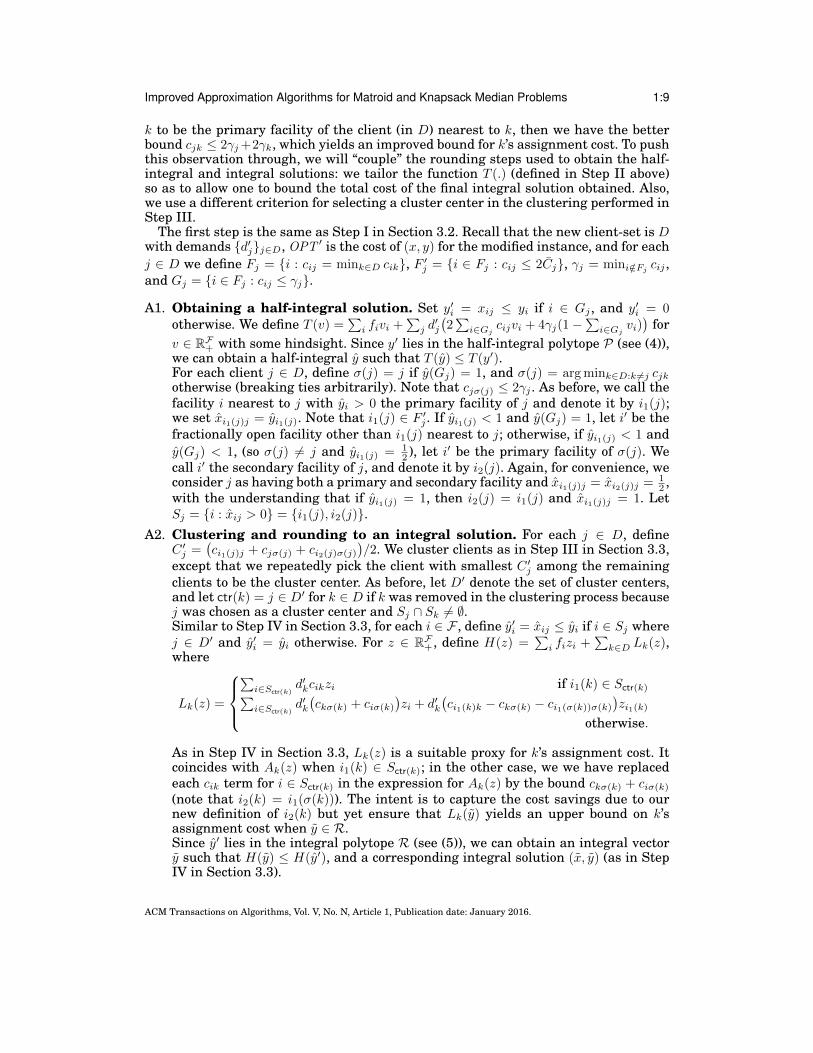
k to be the primary facility of the client (in D) nearest to k, then we have the betterbound cjk ≤ 2γj+2γk, which yields an improved bound for k’s assignment cost. To pushthis observation through, we will “couple” the rounding steps used to obtain the half-integral and integral solutions: we tailor the function T (.) (defined in Step II above)so as to allow one to bound the total cost of the final integral solution obtained. Also,we use a different criterion for selecting a cluster center in the clustering performed inStep III.

The first step is the same as Step I in Section 3.2. Recall that the new client-set is Dwith demands {d′j}j∈D, OPT ′ is the cost of (x, y) for the modified instance, and for eachj ∈ D we define Fj = {i : cij = mink∈D cik}, F ′j = {i ∈ Fj : cij ≤ 2Cj}, γj = mini/∈Fj cij ,and Gj = {i ∈ Fj : cij ≤ γj}.

A1. Obtaining a half-integral solution. Set y′i = xij ≤ yi if i ∈ Gj , and y′i = 0otherwise. We define T (v) =

∑i fivi +

∑j d′j

(2∑i∈Gj cijvi + 4γj(1−

∑i∈Gj vi)

)for

v ∈ RF+ with some hindsight. Since y′ lies in the half-integral polytope P (see (4)),we can obtain a half-integral y such that T (y) ≤ T (y′).For each client j ∈ D, define σ(j) = j if y(Gj) = 1, and σ(j) = arg mink∈D:k 6=j cjkotherwise (breaking ties arbitrarily). Note that cjσ(j) ≤ 2γj . As before, we call thefacility i nearest to j with yi > 0 the primary facility of j and denote it by i1(j);we set xi1(j)j = yi1(j). Note that i1(j) ∈ F ′j . If yi1(j) < 1 and y(Gj) = 1, let i′ be thefractionally open facility other than i1(j) nearest to j; otherwise, if yi1(j) < 1 andy(Gj) < 1, (so σ(j) 6= j and yi1(j) = 1

2 ), let i′ be the primary facility of σ(j). Wecall i′ the secondary facility of j, and denote it by i2(j). Again, for convenience, weconsider j as having both a primary and secondary facility and xi1(j)j = xi2(j)j = 1

2 ,with the understanding that if yi1(j) = 1, then i2(j) = i1(j) and xi1(j)j = 1. LetSj = {i : xij > 0} = {i1(j), i2(j)}.

A2. Clustering and rounding to an integral solution. For each j ∈ D, defineC ′j =

(ci1(j)j + cjσ(j) + ci2(j)σ(j)

)/2. We cluster clients as in Step III in Section 3.3,

except that we repeatedly pick the client with smallest C ′j among the remainingclients to be the cluster center. As before, let D′ denote the set of cluster centers,and let ctr(k) = j ∈ D′ for k ∈ D if k was removed in the clustering process becausej was chosen as a cluster center and Sj ∩ Sk 6= ∅.Similar to Step IV in Section 3.3, for each i ∈ F , define y′i = xij ≤ yi if i ∈ Sj wherej ∈ D′ and y′i = yi otherwise. For z ∈ RF+, define H(z) =

∑i fizi +

∑k∈D Lk(z),

where

Lk(z) =

∑i∈Sctr(k)

d′kcikzi if i1(k) ∈ Sctr(k)∑i∈Sctr(k)

d′k(ckσ(k) + ciσ(k)

)zi + d′k

(ci1(k)k − ckσ(k) − ci1(σ(k))σ(k)

)zi1(k)

otherwise.

As in Step IV in Section 3.3, Lk(z) is a suitable proxy for k’s assignment cost. Itcoincides with Ak(z) when i1(k) ∈ Sctr(k); in the other case, we we have replacedeach cik term for i ∈ Sctr(k) in the expression for Ak(z) by the bound ckσ(k) + ciσ(k)

(note that i2(k) = i1(σ(k))). The intent is to capture the cost savings due to ournew definition of i2(k) but yet ensure that Lk(y) yields an upper bound on k’sassignment cost when y ∈ R.Since y′ lies in the integral polytope R (see (5)), we can obtain an integral vectory such that H(y) ≤ H(y′), and a corresponding integral solution (x, y) (as in StepIV in Section 3.3).


1:10 C. Swamy

Analysis. By mimicking the proof of Lemma 3.2, we easily obtain that T (y′) ≤ 4 ·OPT ′. Hence, we have T (y) ≤ T (y′) ≤ 4 · OPT ′ ≤ 4 · OPT . Lemma 3.6 shows that thecost of (x, y) is at most H(y) ≤ H(y′), and Lemma 3.7 proves that H(y′) ≤ T (y). Thisshows that the cost of (x, y) is at most 4 ·OPT . Combined with Lemma 3.1, this yieldsthe 8-approximation guarantee (Theorem 3.8).

LEMMA 3.6. The cost of (x, y) is at most H(y) ≤ H(y′).

PROOF. The facility opening cost is∑i fiyi. The assignment cost of a client j ∈ D′

is∑i∈Sj d

′jcij yi = Lj(y). Consider a client k ∈ D \D′ with ctr(k) = j. Let i′ = i1(j), i′′ =

i2(j). If yi1(k) = 0 or i1(k) ∈ Sj , then Lk(y) is at least d′k∑i∈Sj cikyi, which is the

assignment cost of k. So suppose yi1(k) = 1 and i1(k) /∈ Sj . Then the assignment cost of kis d′kci1(k)k, and since ciσ(k) ≥ ci1(σ(k))σ(k) for every i ∈ Sj , we have Lk(y) ≥ d′kci1(k)k.

LEMMA 3.7. We have H(y′) ≤ T (y).

PROOF. Define Bj(y) := d′j(2∑i∈Gj cij yi + 4γj(1 − y(Gj))

). So T (y) =

∑i fiyi +∑

j∈D Bj(y). Clearly∑i fiy

′i ≤

∑i fiyi. We show that Lj(y′) ≤ Bj(y) for every j ∈ D,

which will complete the proof.We first argue that d′jC ′j ≤ Bj(y) for every j ∈ D. If y(Gj) = 1, then d′jC

′j =∑

i∈Gj d′jcij yi ≤ Bj(y). Otherwise, y(Gj) = 1

2 , and cjσ(j) + ci1(σ(j))σ(j) ≤ 3γj ; sod′jC

′j ≤ d′j

(∑i∈Gj cij yi + 3γj(1− y(Gj))

)≤ Bj(y).

For a client j ∈ D′, we have Lj(y′) = d′j

(ci1(j)j + ci2(j)j

)/2 ≤ d′jC

′j ≤ Bj(y). Now

consider a client k ∈ D \D′. Let j = ctr(k), and i′ = i1(j), i′′ = i2(j). Note that C ′j ≤ C ′k.We consider two cases.1. i1(k) ∈ Sj . This means that i1(k) = i′′ 6= i′ and k = σ(j). So

Lk(y′) =d′k2·(ci′′k + ci′k

)≤ d′k

2·(ci′j + cjk + ci′′k

)= d′kC

′j ≤ d′kC ′k ≤ Bk(y).

2. i1(k) /∈ Sj . This implies that y(Gk) = yi1(k) = 12 . Let ` = σ(k) (which is the same as j

if i2(k) = i1(j)). We have Lk(y′) =d′k2 ·(2ck`+ ci′`+ ci′′`+ ci1(k)k− ck`− ci1(`)`

). If ` = j,

then Lk(y′) =d′k2 ·(ci1(k)k + cjk + ci′′j

). Notice that ci′′j ≤ 2C ′j− ci′j . So we obtain that

Lk(y′) ≤ d′k2·(ci1(k)k+cjk+2C ′j−ci′j

)≤ d′k

2·(ci1(k)k+cjk+2C ′k−ci′j

)= d′k

(ci1(k)k+cjk

).

If ` 6= j, then i2(j) = i′′ = i2(k) = i1(`), so ` = σ(j), and ci′j + cj`+ ci′′` = 2C ′j ≤ 2C ′k =

ci1(k)k + ck` + ci′′`. So Lk(y′) ≤ d′k2 ·(ci1(k)k + ck` + cj` + ci′j

)≤ d′k(ci1(k)k + ck`). In both

cases,

Lk(y′) ≤ d′k(ci1(k)k + ckσ(k)

)≤ d′k

(2∑i∈Gk

cikyi + 4γk(1− y(Gk)

))= Bk(y).

THEOREM 3.8. The integer solution (x, y) translates to an integer solution to theoriginal instance of cost at most 8 ·OPT .

Remark 3.9. It is easy to modify the above algorithm to obtain a so-calledLagrangian-multiplier preserving (LMP) 8-approximation algorithm, that is, wherethe solution (x, y) returned satisfies 8

∑i fiyi +

∑j∈D,i djcij xij ≤ 8 · OPT . To obtain



this, the only change is that we redefine

T (v) = 8∑i

fivi+∑j

d′j(2∑i∈Gj

cijvi+ 4γj(1−∑i∈Gj

vi)), H(z) = 8

∑i

fizi+∑k∈D

Lk(z).

We now have T (y) ≤ T (y′) ≤ 8∑i fiyi + 4

∑j∈D d

′jCj , and 8

∑i fiyi +

∑j∈D,i d

′jcij xij ≤

H(y) ≤ H(y′). Also, as before, we have H(y′) ≤ T (y). Thus, we have

8∑i

fiyi +∑j∈D,i

djcij xij ≤ 8∑i

fiyi +∑j∈D,i

d′jcij xij +∑

j∈D\D

4djCj

≤ 8∑i

fiyi + 4∑j∈D

djCj + 8∑

j∈D\D

djCj ≤ 8 ·OPT .

4. EXTENSIONS4.1. Matroid median with two matroidsA natural extension of matroid median is the matroid-intersection median problem,wherein are given two matroids on the facility-set F , and we require the set of openfacilities to be an independent set in both matroids. This problem turns out to be in-approximable to within any multiplicative factor in polytime since, as we show in Ap-pendix B, it is NP-complete to determine if there is a zero-cost solution; this holds evenif one of the matroids is a partition matroid.

We consider two extensions of matroid median that are essentially special casesof matroid-intersection median and can be used to model some interesting problems(see Section 5). The techniques developed in Section 3 readily extend and yield an 8-approximation algorithm (in fact, an LMP 8-approximation) for both problems. Theseextensions may be viewed in some sense as the most-general special cases of matroid-intersection median that one can hope to approximately solve in polytime. Technically,the key distinction between (general) matroid-intersection median and the extensionswe consider, which enables one to achieve polytime multiplicative approximation guar-antees for these problems, is the following. In both our extensions, one can definepolytopes analogous to P and R in the earlier rounding procedure (see (4) and (5)respectively) that encode information from the clustering performed in Steps I and IIIrespectively and whose extreme points are defined by equations coming from two lam-inar systems. In contrast, for matroid-intersection median, the extreme points of theanalogous polytopes are defined by equations coming from three laminar systems (oneeach from the two matroids, and one that encodes information about the clusteringstep), which creates an insurmountable obstacle.

The setup in both extensions is similar. We have a matroidM = (F , I) on the facility-set (and clients with demands and assignment costs). F is partitioned into F1∪F2 andclients may only be assigned to facilities in F1; this can be encoded by setting cij = ∞for all i ∈ F2 and j ∈ D. We also have lower and upper bounds (lb1 , ub1 ), (lb2 , ub2 ), and(lb, ub) on the number of facilities that may be opened from F1, F2, and F respectively.As before, we need to open a feasible set of facilities and assign every client to anopen facility so as to minimize the total facility-opening and client-assignment cost.A set F ⊆ F of facilities is said to be feasible if: (i) F ∈ I; (ii) lb1 ≤ |F ∩ F1| ≤ ub1 ,lb2 ≤ |F∩F2| ≤ ub2 , lb ≤ |F | ≤ ub; and (iii) F∩F2 satisfies problem-specific constraints.While the role of F2 may seem unclear, notice that a non-trivial lower bound on thenumber of F2-facilities imposes restrictions on the facilities that may be opened fromF1 due to the matroid M (see, e.g., k-median forest in Section 5).

Two-matroid median (2MMed). In addition to the above setup, we have another ma-troid M2 = (F2, I2) on F2 with rank function r2. A set F of facilities is feasible if it


1:12 C. Swamy

satisfies (i) and (ii) above, and (iii) F ∩F2 ∈ I2. We may modify the matroids M and M2

to incorporate the upper bounds ub and ub2 respectively in their definition; we assumethat this has been done in the sequel. The LP-relaxation for 2MMed is quite similar to(P). We augment (P) with the constraints:

y(S) ≤ r2(S) ∀S ⊆ F2, lb1 ≤ y(F1) ≤ ub1 , lb2 ≤ y(F2), lb ≤ y(F).

Let (x, y) denote an optimal solution to this LP, and OPT denote its cost. The roundingprocedure dovetails the one in Section 3. The first step is again Step I in Section 3.2.Let D be the new client-set with demands {d′j}j∈D, OPT ′ be the new cost of (x, y), andfor each j ∈ D, we define Fj , F ′j , γj , and Gj as before. Note that Fj ⊆ F1 for all j ∈ D.

A slight technicality arises in mimicking Step A1 in Section 3.4: setting y′i = xij forsome facility i ∈ Gj need not satisfy the lower-bound constraints. To deal with this,for every j ∈ D and i ∈ Gj with 0 < xij < yi, we replace facility i with two co-located“clones” i1 and i2. We set fi1 = fi2 = fi, yi1 = xij = xi1j , yi2 = yi − yi1 , xi2j = 0, andfor every client k ∈ D, k 6= j, we arbitrarily split xik into xi1k ≤ yi1 and xi2k ≤ yi2 sothat xi1k+xi2k = xik. We define a new set G′j consisting of the new facilities i for whichcij = mink∈D cik, cij ≤ γj and xij = yi > 0 (that is, G′j consists of the new i1-clones andthe old facilities i ∈ Gj with xij = yi > 0). We continue to let F ′j denote the facilities iwith cij = mink∈D cik and cij ≤ 2Cj . Let F ′1 denote the new F1-set after these changes,and F ′ = F ′1 ∪ F2; the bounds lb1 , ub1 , lb, ub are unchanged. Set h(i) = {i1, i2} ifi is cloned into i1, i2, and h(i) = {i} otherwise. We update the rank function r to r′

(over 2F′) in the obvious way: r′(S) = r

({i ∈ F : h(i) ∩ S 6= ∅}

). Note that r′ defines a

matroid on F ′. Clearly, a solution to the modified translates to a solution to the originalinstance and vice versa.

We continue with steps A1, A2 in Section 3.4, replacing Gj with G′j , and using suit-able polytopes in place of P and R to obtain the half-integral and integral solutions.To obtain a half-integral solution, we define

P ′ :=

{v ∈ RF ′

+ : v(S) ≤ r′(S) ∀S ⊆ F ′, v(S) ≤ r2(S) ∀S ⊆ F2, lb ≤ v(F ′)

lb1 ≤ v(F ′1) ≤ ub1 , lb2 ≤ v(F2), v(F ′j) ≥ 12 , v(G′j) ≤ 1 ∀j ∈ D

}. (6)

Clearly (the new vector) y lies in P ′. The key observation is that an extreme point of P ′is again defined by a linearly independent system of tight constraints coming from twolaminar systems: one consisting of some tight v(S) ≤ r′(S) and lb ≤ v(F ′) ≤ ub con-straints; the other consisting of some tight v(S) ≤ r2(S) and lb1 ≤ v(F ′1) ≤ ub1 , lb2 ≤v(F2) ≤ ub2 constraints, and some tight v(F ′j) ≤ 1

2 and v(G′j) ≥ 1 constraints. Thus,P ′ has half-integral extreme points, and so we can find a half-integral y such thatT (y) ≤ T (y) (where T (.) is as defined in Section 3.4), and a corresponding solution(x, y) as in step A1.

We round (x, y) to an integral solution as in step A2. Recall that Sj = {i : xij > 0}.We define C ′j and cluster clients in D as in step A2 (again using G′j instead of Gj) toobtain the set D′ of cluster centers. A useful observation is that if |Sj | = 1 then wemay assume that j ∈ D′. This is because for any k ∈ D with Sk ∩ Sj 6= ∅, we haveσ(k) = j and therefore C ′k ≥

(cjk + ci1(j)j

)/2 ≥ ci1(j)j = C ′j . Thus, if j ∈ D′, then xij = yi

for all i ∈ Sj : this is clearly true if |Sj | = 1; otherwise, we have that |Sσ(j)| = 2 (since



σ(j) /∈ D′) and so yi1(σ(j)) = 12 . The polytope used to round y is

R′ :=

{z ∈ RF

′

+ : z(S) ≤ r′(S) ∀S ⊆ F ′, z(S) ≤ r2(S) ∀S ⊆ F2,

lb1 ≤ z(F ′1) ≤ ub1 , lb2 ≤ z(F2), lb ≤ z(F ′), z(Sj) = 1 ∀j ∈ D′} (7)

which has integral extreme points. So we obtain an integral vector y such that H(y) ≤H(y) (were H(.) is as defined in in Section 3.4), and hence an integer solution (x, y).Mimicking the analysis in Section 3.4, we obtain that T (y) ≤ T (y) ≤ 4 ·OPT ′, and thecost of (x, y) is at most H(y) ≤ H(y) ≤ T (y). Thus, we obtain the following theorem.

THEOREM 4.1. The integer solution (x, y) yields an integer solution to 2MMed of costat most 8 ·OPT .

Laminarity-constrained matroid median (LCMMed). In LCMMed, in addition to thecommon setup, we have a laminar family L on F2 and bounds 0 ≤ `S ≤ uS for everyset S ∈ L; a set F of facilities is feasible if it satisfies (i) and (ii) above, and (iii) `S ≤|F ∩ S| ≤ uS for all S ∈ L,

The approach used for 2MMed also works for LCMMed. The only (obvious) changesare that the LP-relaxation, as well as the definition of the polytopes P ′ and R′ (in (6)and (7)) now include the laminarity constraints in place of the rank constraints for thesecond matroid. All other steps and arguments proceed identically, and so we obtainan 8-approximation algorithm for laminarity-constrained matroid median.

4.2. Matroid median with penaltiesThis is the generalization of matroid median where are allowed to leave some clientsunassigned at the expense of incurring a penalty djπj for each unassigned client j.This changes the LP-relaxation (P) as follows. We use a variable zj for each clientj ∈ D to denote if we incur the penalty for client j, and modify the assignmentconstraint for client j to

∑i xij + zj ≥ 1; also the objective is now to minimize∑

i fiyi +∑j dj(∑

i cijxij + πjzj). Let (x, y, z) denote an optimal solution to this LP

and OPT be its value.Krishnaswamy et al. [Krishnaswamy et al. 2011] showed that (x, y, z) can be

rounded to an integer solution losing a factor of 360. We show that our roundingapproach for matroid median can be adapted to yield a substantially improved 24-approximation algorithm. The rounding procedure is similar to the one described inSection 3 for matroid median, except that we now need to deal with the complicationthat a client need be assigned fractionally to an extent of 1.

Let Xj =∑i xij , Cj =

∑i cijxij/Xj , and LPj =

∑i cijxij + πjzj = CjXj + πjzj . We

may assume that Xj + zj = 1 for every client j and that if xij > 0 then cij ≤ πj , so wehave Cj ≤ LPj ≤ πj .

Step 0. First, we set zj = 1 and incur the penalty for each client j for which πj ≤ 2LPj .In the sequel, we work with the remaining set D′ = {j ∈ D : 2LPj < πj} of clients. Notethat Xj >

12 for every j ∈ D′. Let OPT ′′ =

∑i fiyi +

∑j∈D′ dj

(∑i cijxij + πjzj

).

Step I: Consolidating demands. We consolidate demands around centers in a man-ner similar to Step I of the rounding procedure in Section 3. The difference is that if kis consolidated with client j, then we cannot simply add dk to j’s demand and replicatej’s assignment for k (since πk could be much larger than πj so that CjXj + πk(1 −Xj)need not be bounded in terms of LPk). Instead, we treat k as being co-located with jand recompute k’s assignment.


1:14 C. Swamy

Let L be a list of clients in D′ arranged in increasing order of LPj . Let D = ∅. Wecompute a new assignment (x′, z′) for the clients as follows. Set x′ij = z′j = 0 for all i, j.Remove the first client j ∈ L and add it to D. Set x′ij = xij for all facilities i and z′j = zj ;also set nbr(j) = j. For every client k in L with cjk ≤ 4LPk, we remove k from L, andset nbr(k) = j. We consider k to be co-located with j and re-optimize k’s assignment.So we set x′ik = yi starting from the facility nearest to j and continuing until k iscompletely assigned or until the last facility i such that cij ≤ πk, in which case we setz′k = 1−

∑i x′ik. Note that

∑i cijx

′ik + πkz

′k ≤

∑i cijxik + πkzk ≤ 4LPk + LPk.

We call each client in D a cluster center. Let {c′ij} denote the assignment costs of theclients with respect to their new locations. Let OPT ′ =

∑i fiyi +

∑j∈D′ dj

(∑i c′ijx′ij +

πjz′j

)denote the cost of the modified solution for the modified instance. The following

lemma is immediate.

LEMMA 4.2. The following hold: (i) if j, k ∈ D′ are not co-located, then cjk ≥4 max(LPj , LPk), (ii) OPT ′ ≤ 5 · OPT ′′, and (iii) any solution to the modified instancecan be converted to a solution to the original instance involving client-set D′ incurringan additional cost of at most 4 ·OPT ′′.

Step II: Obtaining a half-integral solution. As in Step II of Section 3, we define a suit-able vector y′ that lies in a polytope with half-integral extreme points and construct alinear function T (.) with T (y′) = O(OPT ′) bounding the cost of a fractional solution.We can then obtain a “better” half-integral vector y, which yields a half-integral so-lution. In Step III, we round y to an integral solution whose cost we argue is at mostT (y) ≤ T (y′).

Consider a client j ∈ D. Let Fj = {i : cij = mink∈D cik}, F ′j = {i ∈ Fj : cij ≤ 2LPj},γj = mini/∈Fj cij , and Gj = {i ∈ Fj : cij ≤ γj}. Note that

∑i∈F ′

jx′ij =

∑i:cij≤2LPj

x′ij >12

since LPj ≥∑i:cij>2LPj

cijx′ij+πjz

′j (and πj > 2LPj) implies that

∑i:cij>2LPj

x′ij+z′j <12 .

Consider the facilities in Gj in increasing order of their distance from j. For everyfacility i ∈ Gj , we set y′i = min{yi, 1 −

∑i′∈Gj :i′ comes before i y

′i′}. We set y′i = 0 for all

other i ∈ Fj . Note that y′(F ′j) = min{

1, y(F ′j)}≥ 1

2 . Clearly, y′(Fj) = y′(Gj) ≤ 1 and ify(Gj) ≤ 1, then y′i = yi for all i ∈ Gj .

Given v ∈ RF+, for a client k ∈ D′ with nbr(k) = j, we define Bk(v) =

dk(∑

i∈Gj :c′ik≤πk2c′ikvi + min{2πk, 4γj}(1 −

∑i∈Gj :c′ik≤πk

vi)). Now set T (v) =

∑i fivi +∑

j∈D′ Bj(v). Clearly y′ ≤ y, so y′ lies in the polytope P (see (4)), which has half-integralextreme points. So we can obtain a half-integral point y ∈ P ′ such that T (y) ≤ T (y′).

We now obtain a half-integral assignment for the clients in D′ as follows. Consider aclient k and let j = nbr(k). (Note that we could have k = j.) Set σ(j) to be j if y(Gj) = 1,and arg min`∈D: 6=j cj` otherwise (as in Section 3.4). Call the facility i ∈ F ′j nearest toj the primary facility of k, and set xik = yi. If yi < 1, then define i′ to be the facilitynearest to j other than i with yi′ > 0 if y(Gj) = 1, and the primary facility of σ(j)otherwise. If y

({i′′ ∈ Gj : ci′′j ≤ πk}

)= 1

2 and πk ≤ 2γj , we set zk = 12 = 1 − xik.

Otherwise, we set xi′k = 12 = 1− xik and call i′ the secondary facility of k.

Step III: Rounding (x, y) to an integer solution. This step is quite straightforward.We incur the penalty for all clients j ∈ D′ with zj = 1

2 . Note that all the remainingclients k with nbr(k) = j are (co-located and) assigned identically and completely in(x, y, z). Viewing this as an instance with demand consolidated at the cluster centers,we use the rounding procedure in step A2 of Section 3.4 to convert the half-integral so-lution of these remaining clients into an integral one. Let (x, y, z) denote the resultinginteger solution.



LEMMA 4.3. We have T (y) ≤ T (y′) ≤ 4 ·OPT ′.

PROOF. It suffices to show that for every client k, we have Bk(y′) ≤ 4dk(∑

i c′ikx′ik +

πkz′k

). Let j = nbr(k). Consider the facilities in Gj in increasing order of their distance

from j. If πk < γj , then (we may assume that) k uses the facilities in Gj with c′ik =cij ≤ πk fully (i.e., x′ik = yi) until either it is completely assigned (and the last facilityused by k may be partially used) or we exhaust the facilities in Gj with cij ≤ πk. Inboth cases, we have x′ik = y′i for all i ∈ Gj with c′ik ≤ πk and z′k = 1 −


y′i,and so

∑i c′ikx′ik + πkz

′k =


c′iky′i + πk

(1 −


y′i). If πk ≥ γj , then∑

i c′ikx′ik + πkz

′k ≥

∑i∈Gj c

′ikx′ik + γj

(1 −

∑i∈Gj x

′ik

); also, x′ik = y′i for all i ∈ Gj since

πk ≥ c′ik. So in every case, we have Bk(y′) ≤ 4dk(∑

i c′ikx′ik + πkz

′k

).

LEMMA 4.4. The cost of (x, y, z) for the modified instance is at most T (y).

PROOF. Consider a client k and let j = nbr(k). If zk = 1 then Bk(y) ≥ πk, since zk = 12

implies that y(Nk) = 12 , where Nk = {i ∈ Gj : cij ≤ πk}, and πk < 2γj . If zk = 0 then we

claim that Bk(y) = dk(2∑i∈Gj cij yi + 4γj(1 − y(Gj))

). If y(Nk) = 1

2 , then this followssince we must have πk > 2γj for zk to be 0; otherwise, y(Nk) = 1 = y(Gj) and again theequality holds.

The proof of Lemma 3.6 now shows that∑i fiyi +

∑k:zk=0 c

′ikxik ≤ H(y) ≤

∑i fiyi +∑

k:zk=0Bk(y), where H(.) is the function defined in step A2 of Section 3.4 for theinstance where each cluster center j has demand d′j :=

∑k:nbr(k)=jzk=0

dk. Hence, the total

cost of (x, y, z) for the modified instance is at most T (y).

Combined with parts (ii) and (iii) of Lemma 4.2, we obtain a solution to the originalinstance involving client-set D′ of cost at most 24 · OPT ′′. Adding in the penalties ofthe clients in D \D′ (recall that πj ≤ 2LPj for each j ∈ D \D′), we obtain that the totalcost is at most 24 ·OPT .

THEOREM 4.5. One can round (x, y, z) to an integer solution of cost at most 24·OPT .

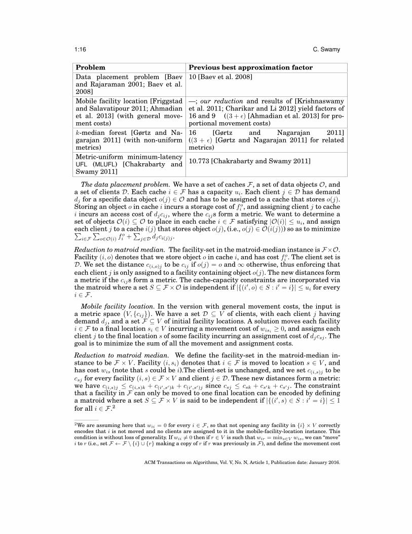
5. APPLICATIONSWe now show that the various facility location problems listed below can be cast asspecial cases of matroid median or the extensions considered in Section 4.1. Thus,our 8-approximation algorithms for matroid median and these extensions immediatelyyield improved approximation guarantees for all these problems.


1:16 C. Swamy

Problem Previous best approximation factorData placement problem [Baevand Rajaraman 2001; Baev et al.2008]

10 [Baev et al. 2008]

Mobile facility location [Friggstadand Salavatipour 2011; Ahmadianet al. 2013] (with general move-ment costs)

—; our reduction and results of [Krishnaswamyet al. 2011; Charikar and Li 2012] yield factors of16 and 9 ((3 + ε) [Ahmadian et al. 2013] for pro-portional movement costs)

k-median forest [Gørtz and Na-garajan 2011] (with non-uniformmetrics)

16 [Gørtz and Nagarajan 2011]((3 + ε) [Gørtz and Nagarajan 2011] for relatedmetrics)

Metric-uniform minimum-latencyUFL (MLUFL) [Chakrabarty andSwamy 2011]

10.773 [Chakrabarty and Swamy 2011]

The data placement problem. We have a set of caches F , a set of data objects O, anda set of clients D. Each cache i ∈ F has a capacity ui. Each client j ∈ D has demanddj for a specific data object o(j) ∈ O and has to be assigned to a cache that stores o(j).Storing an object o in cache i incurs a storage cost of foi , and assigning client j to cachei incurs an access cost of djcij , where the cijs form a metric. We want to determine aset of objects O(i) ⊆ O to place in each cache i ∈ F satisfying |O(i)| ≤ ui, and assigneach client j to a cache i(j) that stores object o(j), (i.e., o(j) ∈ O(i(j))) so as to minimize∑i∈F

∑o∈O(i) f

oi +

∑j∈D djci(j)j .

Reduction to matroid median. The facility-set in the matroid-median instance is F×O.Facility (i, o) denotes that we store object o in cache i, and has cost foi . The client set isD. We set the distance c(i,o)j to be cij if o(j) = o and ∞ otherwise, thus enforcing thateach client j is only assigned to a facility containing object o(j). The new distances forma metric if the cijs form a metric. The cache-capacity constraints are incorporated viathe matroid where a set S ⊆ F ×O is independent if |{(i′, o) ∈ S : i′ = i}| ≤ ui for everyi ∈ F .

Mobile facility location. In the version with general movement costs, the input isa metric space

(V, {cij}

). We have a set D ⊆ V of clients, with each client j having

demand dj , and a set F ⊆ V of initial facility locations. A solution moves each facilityi ∈ F to a final location si ∈ V incurring a movement cost of wisi ≥ 0, and assigns eachclient j to the final location s of some facility incurring an assignment cost of djcsj . Thegoal is to minimize the sum of all the movement and assignment costs.

Reduction to matroid median. We define the facility-set in the matroid-median in-stance to be F × V . Facility (i, si) denotes that i ∈ F is moved to location s ∈ V , andhas cost wis (note that s could be i).The client-set is unchanged, and we set c(i,s)j to becsj for every facility (i, s) ∈ F ×V and client j ∈ D. These new distances form a metric:we have c(i,s)j ≤ c(i,s)k + c(i′,s′)k + c(i′,s′)j since csj ≤ csk + cs′k + cs′j . The constraintthat a facility in F can only be moved to one final location can be encoded by defininga matroid where a set S ⊆ F × V is said to be independent if |{(i′, s) ∈ S : i′ = i}| ≤ 1for all i ∈ F .2

2We are assuming here that wii = 0 for every i ∈ F , so that not opening any facility in {i} × V correctlyencodes that i is not moved and no clients are assigned to it in the mobile-facility-location instance. Thiscondition is without loss of generality. If wii 6= 0 then if r ∈ V is such that wir = mins∈V wis, we can “move”i to r (i.e., set F ← F \ {i} ∪ {r} making a copy of r if r was previously in F ), and define the movement cost



k-median forest. In the non-uniform version, we have two metric spaces(V, {cuv}

)and

(V, {duv}

). The goal is to find S ⊆ V with |S| ≤ k and assign every node j ∈ V to

i(j) ∈ S so as to minimize∑j ci(j)j + d

(MST(V/S)

), where MST(V/S) is a minimum

spanning forest where each component contains a node of S.

Reduction to 2MMed (or LCMMed). We actually reduce a generalization, where there isan “opening cost” fi ≥ 0 incurred for including i in S; the resulting instance is alsoan LCMMed instance. We add a root r to V . The facility-set F is the edge-set of thecomplete graph on V ∪ {r}. The client-set is D := V . Selecting a facility (r, i) denotesthat i ∈ S, and selecting a facility (u, v), where u, v 6= r, denotes that (u, v) is part ofMST(V/S). We let F1 be the edges incident to r, and F2 be the remaining edges. Thecost of a facility (r, i) ∈ F1 is fi; the cost of a facility (u, v) ∈ F2 is duv. The client-facilitydistances are given by c(r,i)j = cij and cej = ∞ for every e ∈ F2. Note that these {cej}distances form a metric. We let M be the graphic matroid of the complete graph onV ∪{r}. We impose a lower bound of |V | on the number of facilities opened from F , andan upper bound of k on the number of facilities opened from F1. The matroid M2 on F2

is the vacuous one where every set is independent.A feasible solution to the 2MMed instance corresponds to a spanning tree on V ∪ {r}

where r has degree at most k. This yields a solution to k-median forest of no-greatercost, where the set S is the set of nodes adjacent to r in this edge-set. Conversely, it iseasy to see that a solution S to the k-median forest instance yields a 2MMed solution ofno-greater cost.

Metric uniform MLUFL. We have a set F of facilities with opening costs {fi}i∈F , anda set D of clients with assignment costs {cij}j∈D,i∈F , where the cijs form a metric.Also, we have a monotone latency-cost function λ : Z+ 7→ R+. The goal is to choose aset F ⊆ F of facilities to open, assign each open facility i ∈ F a distinct time-indexti ∈ {1, . . . , |F|}, and assign each client j to an open facility i(j) ∈ F so as to minimize∑i∈F fi +

∑j∈D

(ci(j)j + λ(ti(j))

).

Reduction to matroid median. We define the facility-set to be F × {1, . . . , |F|} and thematroid on this set to encode that a set S is independent if |{(i, t′) ∈ S : t′ = t}| ≤ 1 forall t ∈ {1, . . . , |F|}. We set f(i,t) = fi and c(i,t),j = cij + λ(t); note that these distancesform a metric. It is easy to see that we can convert any matroid-median solution to onewhere we open at most one (i, t) facility for any given i without increasing the cost, andhence, the matroid-median instance correctly encodes metric uniform MLUFL.

6. KNAPSACK MEDIANWe now consider the knapsack median problem [Krishnaswamy et al. 2011; Kumar2012], wherein instead of a matroid on the facility-set, we have a knapsack constrainton the facility-set. Kumar [Kumar 2012] obtained the first constant-factor approxi-mation algorithm for this problem, and [Charikar and Li 2012] obtained an improved34-approximation algorithm. We consider a somewhat more-general version of knap-sack median, wherein each facility i has a facility-opening cost fi and a weight wi,and we have a knapsack constraint

∑i∈F wi ≤ B constraining the total weight of open

facilities. We leverage the ideas from our simpler improved rounding procedure for ma-troid median to obtain an improved 32-approximation algorithm for this (generalized)knapsack-median problem. We show that one can obtain a nearly half-integral solu-tion whose cost is within a constant-factor of the optimum. It then turns out to be easy

of r to be w′rs = wis − wir for all s ∈ V . It is easy to see that a ρ-approximate solution to the new instance

translates to a ρ-approximate solution to the original instance.


1:18 C. Swamy

to round this to an integral solution. The resulting algorithm and analysis is simplerthan that in [Kumar 2012; Charikar and Li 2012]. We defer the details to Appendix C.

APPENDIXA. ALTERNATE PROOF OF HALF-INTEGRALITY OF THE POLYTOPE P DEFINED BY (4)We give an alternate proof of half-integrality of P based on the integrality of the inter-section of two submodular polyhedra. Observe that by setting zi = 2vi for i ∈ F , andintroducing slack variables sj for every j ∈ D, the system defining P is equivalent to

0 ≤ z(S) ≤ 2r(S) ∀S ⊆ F , z(Gj) + sj = 2, z(Gj \ F ′j) + sj ≤ 1, sj ≥ 0 ∀j ∈ D. (8)

This in turn is equivalent to

z(S) + s(A) ≤ h1(S ]A) ∀S ⊆ F , A ⊆ D (9)z(S) + s(A) ≤ h2(S ]A) ∀S ⊆ F , A ⊆ D (10)

z, s ≥ 0 (11)z(Gj) + sj = 2 ∀j ∈ D (12)

where h1 and h2 are submodular functions defined over F ] D given by h1(S ] A) :=2r(S)+|A| and h2(S]A) := 2|{j : F ′j∩S 6= ∅}|+|{j : F ′j∩S = ∅ and (j ∈ A or Gj∩S 6= ∅)}|.(To see the equivalence, it is clear that constraints (9)–(12) include (8). Conversely, (9)follows by adding the constraints z(S) ≤ 2r(S) and sj ≤ 1 for all j ∈ A; (10) is impliedby the sum of constraints z(Gj)+sj = 2 for all j such that F ′j∩S 6= ∅, and z(Gj)+sj ≤ 1for all other j such that j ∈ A or Gj ∩ S 6= ∅.) Let Q be the polytope defined by (9)–(11). Since h1 and h2 are integer submodular functions, Q is the intersection of thesubmodular polyhedra for h1 and h2, which is known to be integral. Also, constraints(9)–(12) define a face of Q. Now it is easy to see that an extreme point v of P, maps toan extreme point (2v, s), for a suitably defined s, of this face (which must be integral).Hence, P has half-integral extreme points.

B. INAPPROXIMABILITY OF MATROID-INTERSECTION MEDIANWe show that the problem of deciding if an instance of matroid-intersection medianhas a zero-cost solution is NP-complete. This implies that no multiplicative approxi-mation factor is achievable in polytime for this problem unless P=NP. The reductionis from the NP-complete directed Hamiltonian path problem, wherein we are given adirected graph D = (N,A), and two nodes s, t, and we need to determine if there isa simple (directed) s ; t path spanning all the nodes. The facility-set in the matroid-intersection median problem is the arc-set A, and every node except t is a client. Oneof the matroids M is the graphic matroid on the undirected version of D, that is, anarc-set is independent if it is acyclic when we ignore the edge directions. The secondmatroid M2 is a partition matroid that enforces that every node other than s has atmost one incoming arc. All facility-costs are 0. We set cij = 0 if i is an outgoing arc of j,and∞ otherwise. Notice that this forms a metric since the sets {i : cij = 0} are disjointfor different clients.

It is easy to see that an s ; t Hamiltonian path translates to a zero-cost solution tothe matroid-intersection median problem. Conversely, if we have a zero-cost solutionto matroid-intersection median, then it must open |N |−1 facilities, one for each client.Hence, the resulting edges must form a (spanning) arborescence rooted at s, and more-over, every node other than t must have an outgoing arc. Thus, the resulting edgesyield an s; t Hamiltonian path.



C. KNAPSACK MEDIAN: ALGORITHM DETAILS AND ANALYSISRecall that we consider a more general version of knapsack median than that consid-ered in [Krishnaswamy et al. 2011; Kumar 2012; Charikar and Li 2012]. Each facilityi has a facility-opening cost fi and a weight wi, and we have a knapsack constraint∑i∈F wi ≤ B constraining the total weight of open facilities. The goal is to minimize

the sum of the facility-opening and client-connection costs while satisfying the knap-sack constraint on the set of open facilities. We may assume that we know the max-imum facility-opening cost fopt of a facility opened by an optimal solution, so in thesequel we assume that fi ≤ fopt , wi ≤ B for all facilities i ∈ F .

Krishnaswamy et al. [Krishnaswamy et al. 2011] showed that the natural LP-relaxation for knapsack median has a bad integrality gap; this holds even after aug-menting the natural LP with knapsack-cover inequalities. To circumvent this diffi-culty, Kumar [Kumar 2012] proposed the following lower bound, which we also use.Suppose that we have an estimate Copt within a (1 + ε)-factor of the connection cost ofan optimal solution (which we can obtain by enumerating all powers of (1 + ε)). Then,defining Uj := arg max{z :

∑k dk max{0, z − cjk} ≤ Copt}, Kumar argued that the con-

straint xij = 0 if cij > Uj is valid for the knapsack median instance. We augment thenatural LP-relaxation with these constraints to obtain the following LP (K-P).

min∑i

fiyi +∑j

∑i

djcijxij (K-P)

s.t.∑i

xij ≥ 1 ∀j

xij ≤ yi ∀i, j∑i

wiyi ≤ B

xij , yi ≥ 0 ∀i, j; xij = 0 if cij > Uj .

Let (x, y) be an optimal solution to (K-P) and OPT be its value. Let Cj =∑i cijxij .

Note that if our estimate Copt is correct, then OPT is at most the optimal value optfor the knapsack median instance. We show that (x, y) can be rounded to an integersolution of cost fopt + 4Copt + 28 · OPT . Thus, if consider all possible choices for Copt

in powers of (1 + ε) and pick the solution returned with least cost, we obtain a solutionof cost at most (32 + ε) times the optimum. The rounding procedure is as follows.

K1. Consolidating demands. We start by consolidating demands as in Step I inSection 3.2. We now work with the client set D and the demands {d′j}j∈D. Forj ∈ D, we use Mj ⊆ D to denote the set of clients (including j) whose demandswere moved to j. Note that the Mjs partition D. Let OPT ′ denote the cost of (x, y)for this modified instance. As before, for each j ∈ D we define Fj = {i : cij =mink∈D cik}, F ′j = {i ∈ Fj : cij ≤ 2Cj}, γj = mini/∈Fj cij , and Gj = {i ∈ Fj : cij ≤ γj}.

K2. Obtaining a nearly half-integral solution. Set y′i = xij ≤ yi if i ∈ Gj , andy′i = 0 otherwise. Let F ′ =

⋃j∈D Gj . In the sequel, we will only consider facilities

in F ′. Consider the following polytope:

K :={v ∈ RF

′

+ : v(F ′j) ≥ 12 , v(Gj) ≤ 1 ∀j ∈ D,

∑i

wivi ≤ B}. (13)

Define K(v) =∑i 2fivi +

∑j d′j

(2∑i∈Gj cijvi + 8γj(1 − v(Gj))

)for v ∈ RF ′

+ . Sincey′ ∈ K, we can efficiently obtain an extreme point y of K such that K(y) ≤ K(y′),the support of y is a subset of the support of y′, and all constraints that are tight


1:20 C. Swamy

under y′ remain tight under y.3 Thus, if i ∈ Gj and yi > 0, then y′i > 0 and socij ≤ Uj . Also, if y(Gj) < 1 then y′(Gj) < 1, and so γj ≤ Uj . We show in Lemma C.1that there is at most one client, which we call the special client and denote by s,such that Gs contains a facility i with yi /∈

{0, 1

2 , 1}

.As in Section 3.4, for each client j ∈ D, define σ(j) = j if y(Gj) = 1, and σ(j) =arg mink∈D:k 6=j cjk otherwise (breaking ties arbitrarily). Note that cjσ(j) ≤ 2γj . Wenow define the primary and secondary facilities of each client j ∈ D, which wedenote by i1(j) and i2(j) respectively. If j is not the special client s, then i1(j)is the facility i nearest to j with yi > 0; otherwise, i1(j) = arg mini∈F ′

j :yi>0 wi(breaking ties arbitrarily). If yi1(j) = 1, then we set i2(j) = i1(j). If y(Gj) < 1, weset i2(j) = i1(σ(j)). If yi1(j) < y(Gj) = 1, we set i2(j) to: the half-integral facilityin Gj other than i1(j) that is nearest to j if j 6= s; and the facility with smallestweight among the facilities i ∈ Gj with yi > 0 (which could be the same as i1(j)) ifj = s. Define Sj = {i1(j), i2(j)}.To gain some intuition, observe that the facilities i1(j) and i2(j) naturally yielda half-integral solution, where these facilities are open to an extent of 1

2 and j isassigned to them to an extent of 1

2 ; as before, if i1(j) = i2(j), then this means thati1(j) is open to an extent of 1 and j is assigned completely to i1(j). The choice ofthe primary and secondary facilities ensures that this solution is feasible. (We donot however modify y as indicated above.)

K3. Clustering and rounding to an integral solution. This step is quite straight-forward. We define C ′j for j ∈ D, and cluster clients in D exactly as in step A2in Section 3.4, and we open the facility with smallest weight within each cluster.Finally, we assign each client to the nearest open facility. Let (x, y) denote the re-sulting solution. Recall that D′ is the set of cluster centers, and for k ∈ D, ctr(k)denotes the client in D due to which k was removed in the clustering process (soctr(j) = j for j ∈ D′).

Analysis. We call a facility i half-integral (with respect to the vector y obtained instep K2) if yi ∈ {0, 1

2 , 1} and fractional otherwise.

LEMMA C.1. The extreme point y of K obtained in step K2 is such that there isat most one client, called the special client and denoted by s, such that Gs containsfractional facilities. Moreover, if 1

2 < y(Gs) < 1, then there is one exactly one facilityi ∈ F ′s such that yi > 0.

PROOF. Since y is an extreme point, it is well known that the submatrix A′ of theconstraint matrix whose columns correspond to the non-zero yis and rows correspondto the tight constraints under y has full column-rank. The rows and columns of A′ maybe accounted for as follows. Each client j ∈ D contributes: (i) a non-empty disjoint setof columns corresponding to the positive yis in Gj ; and (ii) a possibly-empty disjointset of at most two rows corresponding to the tight constraints y(F ′j) = 1

2 and y(Gj) = 1.This accounts for all columns of A′. There is at most one remaining row of A′, whichcorresponds to the tight constraint

∑i wiyi = B.

3We can obtain y as follows. Let Av ≤ b, v ≥ 0 denote the constraints of K. Recall that z is an extreme pointof K iff the submatrix A′ of A corresponding to the non-zero variables and the tight constraints has fullcolumn rank. So if y′ is not an extreme point, then letting F ′′ = {i : y′i > 0}, we can find some d′ ∈ RF′′

such that A′d = 0. So letting di = d′i if i ∈ F ′′ and 0 otherwise, we can find some ε > 0 such that both y′+εdand y′− εd are feasible and all constraints that were tight under y′ remain tight. So moving in the directionthat does not increase the K(.)-value until some non-zero y′i drops down to 0 or some new constraint goestight, and repeating, we obtain the desired extreme point y.



Let pj and qj denote respectively the number of columns and rows contributed byj ∈ D. First, note that pj ≥ qj for all j ∈ D. This is clearly true if qj ≤ 1; if qj = 2, theny(F ′j) = 1

2 , y(Gj) = 1, so both F ′j and Gj must have at least one positive yi. Also, notethat if pj = qj , then Gj contains only half-integral facilities. Since

∑j pj ≤

∑j qj + 1,

there can be at most one client such that pj > qj ; we let this be our special client s.Note that we must have ps = qs + 1.

If 12 < y(Gs) < 1 then: (i) qs = 0, so ps = 1; or (ii) qs = 1, so ps = 2, and since

y(F ′s) = 12 < y(Gs), both F ′s and Gs contain exactly one positive yi.

It is easy to adapt the proof of Lemma 3.2, and obtain thatK(y) ≤ K(y′) ≤ 8·OPT ′ ≤8 ·OPT . Next, we prove our main result: the integer solution (x, y) computed is feasibleand its cost for the modified instance is at most K(y) + fopt + 4Copt + 16 ·OPT . Thus,“moving” the consolidated demands back to their original locations yields a solution ofcost at most (32 + ε) · opt for the correct guess of fopt and Copt . The following claimswill be useful.

CLAIM C.2. If y(Gj) = 1 for some j ∈ D, then (we may assume that) j is a clustercenter.

PROOF. Let i′ = i1(j), i′′ = i2(j). Let k ∈ D be such that Sk ∩ Sj 6= ∅. Then σ(k) = j.So 2(C ′k − C ′j) = ci1(k)k + cjk − ci2(j)j ≥ ci1(k)j − ci2(j)j ≥ 0 since i2(k) /∈ Gj .

CLAIM C.3. For any client j ∈ D, we have d′jUj ≤ Copt + 4 ·OPT .

PROOF. By definition,∑k dk max{0, Uj − cjk} ≤ Copt . So d′jUj =

∑k∈Mj

dkUj , whichequals ∑

k∈Mj

dk(Uj − cjk) +∑k∈Mj

dkcjk ≤ Copt +∑k∈Mj

4dkCk ≤ Copt + 4 ·OPT .

THEOREM C.4. The solution (x, y) computed in step K3 for the modified instance isfeasible and has cost at most K(y) + fopt + 4Copt + 16 ·OPT .

PROOF. Let Bj(v) = d′j(2∑i∈Gj cijvi + 8γj(1 − v(Gj)) for v ∈ RF ′

+ . So K(y) =

2∑i fiyi +

∑j Bj(y). Recall that Sj = {i1(j), i2(j)} for every j ∈ D.

We first prove feasibility and bound the total facility-opening cost. Consider a clustercentered at j. Let i′ = i1(j), i′′ = i2(j). Let i be the facility opened from Sj . If y(Sj) = 1,then wi ≤

∑i∈Sj wiyi. Otherwise, either j = s or σ(j) = s. If j = σ(j) = s, then i is

the least-weight facility in Gj . Otherwise, if j = s then i is the least-weight facilityin F ′j ∪ {i2(j)} and y(F ′j) + yi2(j) ≥ 1; finally, if j 6= σ(j) = s then i is the least-weightfacility in {i1(j)} ∪ F ′σ(j) and yi1(j) + y(F ′σ(j)) ≥ 1. Since Sj ⊆ Gj ∪ Gσ(j), in every case,we have wi ≤

∑i∈Gj∪Gσ(j) wiyi.

If all facilities in Sj are half-integral, then fi ≤ 2∑i∈Sj fiyi ≤ 2

∑i∈Gj∪Gσ(j) fiyi.

Otherwise, we have j = s or σ(j) = s, and we bound fi by fopt .Note that if k ∈ D′ is some other cluster center, then Gj ∪ Gσ(j) is disjoint from

Gk ∪Gσ(k). If not, then we must have σ(j) = k or σ(k) = j or σ(j) = σ(k), which yieldsthe contradiction that Sj ∩ Sk 6= ∅. So summing over all clusters, we obtain that thetotal weight of open facilities is at most

∑j∈D′

∑i∈Gj∪Gσ(j) wiyi ≤

∑i wiyi ≤ B, and

the facility opening cost is at most 2∑i fiyi + fopt .


1:22 C. Swamy

We now bound the total client-assignment cost. Fix a client j ∈ D′. The assignmentcost of j is at most d′jci2(j)j . Note that ci2(j)j ≤ 3Uj . If j 6= s, then Bj(y) ≥ d′jci2(j)j : thisholds if y(Gj) = 1 since yi2(j) ≥ 1

2 ; otherwise, Bj(y) ≥ 4d′jγj ≥ d′jci2(j)j . If j = s, then itsassignment cost is at most 3d′jUj ≤ 3Copt + 12 ·OPT (Claim C.3).

Now consider k ∈ D \ D′. Let j = ctr(k), and i′ = i1(j), i′′ = i2(j). We consider twocases.1. i1(k) ∈ Sj . Then k = σ(j) and k’s assignment cost is at most d′kci2(k)k. As above, this

is bounded by Bk(y) if k 6= s, and by 3Copt + 12 ·OPT otherwise.2. i1(k) /∈ Sj . Let ` = σ(k). We claim that the assignment cost of k is at most d′k

(ci1(k)k+

4γk). To see this, first suppose ` 6= j, and so ` = σ(j). Then, k’s assignment cost is

at most d′k(ck` + c`j + ci′j

)≤ d′k

(2ck` + ci1(k)k

)≤ d′k

(ci1(k)k + 4γk

), where the first

inequality follows since C ′j ≤ C ′k. If ` = j, then i2(k) = i1(j) = i′ and k’s assignmentcost is at most d′k

(cjk + cjσ(j) + ci2(j)σ(j)

)≤ d′k

(ci1(k) + 2cjk

)≤ d′k

(ci1(k)k + 4γk

), where

the first inequality again follows from C ′j ≤ C ′k.Since k /∈ D′, we have y(Gk) < 1 (by Claim C.2). So y′(Gk) < 1 and γk ≤ Uk.If k 6= s, then Bk(y) ≥ d′k

(ci1(k)k + 4γk

). If k = s and y(Gk) = 1

2 , then Bk(y) ≥4d′kγk and d′kci1(k)k ≤ d′kUk. Otherwise, by Lemma C.1, we have yi1(k) >

12 , and so

Bk(y) ≥ d′kci1(k)k and 4d′kγk ≤ 4d′kUk. Taking all cases into account, we can bound k’sassignment cost by Bk(y) if k 6= s, and by Bk(y) + 4d′kUk ≤ Bk(y) + 4Copt + 16 ·OPTif k = s.

Putting everything together, the total cost of (x, y) is at most 2∑i fiyi +

∑j Bj(y) +

fopt + 4Copt + 16 ·OPT = K(y) + fopt + 4Copt + 16 ·OPT .

COROLLARY C.5. There is a (32 + ε)-approximation algorithm for the knapsackmedian problem.

ACKNOWLEDGMENTS

I thank Deeparnab Chakrabarty for various stimulating discussions that eventually led to this work. I thankChandra Chekuri for some useful discussions regarding the matroid-intersection median problem.

REFERENCESS. Ahmadian, Z. Friggstad, and C. Swamy. 2013. Local-search based approximation algorithms for mobile

facility location problems. In Proceedings of the 24th Annual ACM-SIAM Symposium on Discrete Algo-rithms (SODA). 1607–1621.

I. Baev and R. Rajaraman. 2001. Approximation algorithms for data placement in arbitrary networks.(2001), 661–670.

I. Baev, R. Rajaraman, and C. Swamy. 2008. Approximation algorithms for data placement problems. SIAMJ. Comput. 38, 4 (2008), 1411–1429.

D. Chakrabarty and C. Swamy. 2011. Facility location with client latencies: linear-programming based tech-niques for minimum latency problems. In Proceedings of the 15th International Conference on IntegerProgramming and Combinatorial Optimization (IPCO). 92–103.

M. Charikar, S. Guha, E. Tardos, and D. B. Shmoys. 2002. A constant-factor approximation algorithm forthe k-median problem. J. Comput. System Sci. 65, 1 (2002), 129–149.

M. Charikar and S. Li. 2012. A dependent LP-rounding approach for the k-median problem. In Proceedingsof the 39th International colloquium on Automata, Languages and Programming ICALP. 194–205.

F. Chudak and D. Shmoys. 2003. Improved approximation algorithms for the uncapacitated facility locationproblem. SIAM J. Comput. 33 (2003), 1–25.

W. Cook, W. Cunningham, W. Pulleyblank, and A. Schrijver. 1998. Combinatorial Optimization. John Wileyand Sons, Inc., New York.



Z. Friggstad and M. Salavatipour. 2011. Minimizing movement in mobile facility location problems. ACMTransactions on Algorithms 7, 3, Article 28 (2011), 22 pages.

I. Gørtz and V. Nagarajan. 2011. Locating depots for capacitated vehicle routing. In Proceedings of the 14thInternational Workshop on Approximation Algorithms for Combinatorial Optimization APPROX. 230–241.

R. Krishnaswamy, A. Kumar, V. Nagarajan, Y. Sabharwal, and B. Saha. 2011. The matroid median problem.In Proceedings of the 22nd Annual ACM-SIAM Symposium on Discrete Algorithms (SODA). 1117–1130.

A. Kumar. 2012. Constant-factor approximation algorithm for the knapsack median problem. In Proceedingsof the 23rd Annual ACM-SIAM Symposium on Discrete Algorithms (SODA). 824–832.

D. B. Shmoys, E. Tardos, and K. I. Aardal. 1997. Approximation algorithms for facility location problems. InProceedings of the 29th Annual ACM Symposium on Theory of Computing (STOC). 265–274.

C. Swamy. 2014. Improved approximation algorithms for matroid and knapsack median problems and ap-plications. In Proceedings of the 17th International Workshop on Approximation Algorithms for Combi-natorial Optimization (APPROX). 403–418.

C. Swamy and D. B. Shmoys. 2008. Fault-tolerant facility location. ACM Transactions on Algorithms 4, 4,Article 51 (2008), 27 pages.


Documents

1 Improved Approximation Algorithms for Matroid and ...cswamy/papers/mmed-journ.pdf · Improved Approximation Algorithms for Matroid and Knapsack ... Improved Approximation Algorithms