Embed Size (px)
Citation preview
COMBINATORICABolyai Society – Springer-Verlag
COMBINATORICA 18 (2) (1998) 151–171
APPROXIMATING PROBABILITY DISTRIBUTIONS USING SMALLSAMPLE SPACES
YOSSI AZAR*, RAJEEV MOTWANI† and JOSEPH (SEFFI) NAOR‡
Received September 22, 1990
First revision November 11, 1990; last revision November 10, 1997
Dedicated to the memory of Paul Erdos
We formulate the notion of a “good approximation” to a probability distribution over afinite abelian group G. The quality of the approximating distribution is characterized by aparameter ε which is a bound on the difference between corresponding Fourier coefficients ofthe two distributions. It is also required that the sample space of the approximating distributionbe of size polynomial in log |G| and 1/ε. Such approximations are useful in reducing or eliminatingthe use of randomness in certain randomized algorithms.
We demonstrate the existence of such good approximations to arbitrary distributions. In thecase of n random variables distributed uniformly and independently over the range 0, . . . ,d−1,we provide an efficient construction of a good approximation. The approximation constructed hasthe property that any linear combination of the random variables (modulo d) has essentially thesame behavior under the approximating distribution as it does under the uniform distribution over0, . . . ,d−1. Our analysis is based on Weil’s character sum estimates. We apply this result tothe construction of a non-binary linear code where the alphabet symbols appear almost uniformlyin each non-zero code-word.
1. Introduction
Recently a family of techniques has emerged to reduce or eliminate the use of ran-dom bits by randomized algorithms [2, 7, 8, 18, 21, 22, 23, 25]. Typically, thesetechniques involve substituting independent random variables by a collection of de-pendent random variables which can be generated using fewer truly independent
Mathematics Subject Classification (1991): 60C05, 60E15, 68Q22, 68Q25, 68R10, 94C12
* Part of this work was done while the author was at the Computer Science Department,
Stanford University and supported by a Weizmann fellowship and Contract ONR N00014-88-K-0166.† Supported by an Alfred P. Sloan Research Fellowship, an IBM Faculty Development Award,
grants from Mitsubishi Electric Laboratories and OTL, NSF Grant CCR-9010517, and NSF Young
Investigator Award CCR-9357849, with matching funds from IBM, Schlumberger Foundation,Shell Foundation, and Xerox Corporation.‡ Part of this work was done while the author was visiting the Computer Science Department,
Stanford University, and supported by Contract ONR N00014-88-K-0166, and by Grant No. 92-00225 from the United States-Israel Binational Science Foundation (BSF), Jerusalem, Israel.
0209–9683/98/$6.00 c©1998 Janos Bolyai Mathematical Society
152 YOSSI AZAR, RAJEEV MOTWANI, JOSEPH (SEFFI) NAOR
random bits. Motivated by this work, we formulate the notion of a good approxi-mation to a joint probability distribution of a collection of random variables.
We consider probability distributions over a finite abelian group G and, in par-ticular, over Znd for any positive integers d and n. We measure the distance betweentwo distributions over G by the distance, in the maximum norm, of their Fouriertransforms over G. Given an arbitrary distribution D over G, a good approxima-tion D is a distribution with a small distance to D, which is concentrated on a smallsubset of the sample space. Sampling from the approximating distribution requiressignificantly fewer random bits than sampling from the original distribution.
Before describing our work in detail, we briefly review some related work. Alon,Babai, and Itai [2] and Luby [21] observed that certain algorithms perform as wellusing pairwise independent random bits, as on mutually independent bits. It turnsout that n uniform k-wise independent bits can be generated using sample spaces ofsize O(nbk/2c); a lower bound of
( nbk/2c
)on the minimum size of such a sample space
is also known [2, 9]. Thus, these algorithms could be derandomized for constantk by an exhaustive search of the (polynomial-size) sample space. Unfortunately,this degree of independence is very restrictive and limits the applicability of theapproach. Berger and Rompel [7] and Motwani, Naor, and Naor [23] showedthat several interesting algorithms perform reasonably well with only (logn)-wiseindependence. The resulting sample space, while of super-polynomial size, couldbe efficiently searched via the method of conditional probabilities, due to Erdos andSelfridge [12] (cf. [3, Chapter 15]), in time logarithmic in the size of the samplespace. This led to the derandomization of a large class of parallel algorithms [7,23].
An alternate approach was proposed by Naor and Naor [25] based on the notionof the bias of a distribution due to Vazirani [28].
Definition 1.1. Let X1, . . . ,Xn be 0,1 random variables. The bias of a subset S ofthe random variables is defined to be
∣∣Pr[∑
i∈SXi=0]−Pr
[∑i∈SXi=1
]∣∣, wherethe sum is taken modulo 2.
For mutually independent and uniform random variables, the bias of each non-empty subset is zero. It is not hard to show that the converse holds as well. Inan ε-biased probability distribution, each subset of the random variables has biasat most ε. Naor and Naor [25] showed how to construct such a distribution, forany ε > 0, such that the size of the sample space is polynomial in n and 1/ε.The ε-biased distribution can be viewed as an almost (logn)-wise independentdistribution. A result due to Peralta [26] implies a different construction of ε-biased probability distribution using the properties of quadratic residues; this andtwo additional constructions of two-valued ε-biased random variables are reportedby Alon, Goldreich, Hastad, and Peralta [1].
We formulate and study the notion of a “good approximation” to a joint prob-ability distribution of (possibly multi-valued) random variables. Let D be any jointdistribution of n random variables over the range 0, . . . ,d−1. Informally, a goodapproximation D to D satisfies the following properties: there is a uniform bound
APPROXIMATING PROBABILITY DISTRIBUTIONS USING SMALL SAMPLE SPACES 153
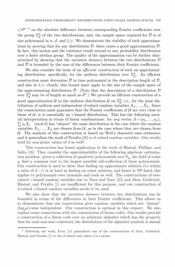
ε/dn−1 on the absolute difference between corresponding Fourier coefficients overthe group Znd of the two distributions; and, the sample space required for D is ofsize polynomial in n, d, and 1/ε. We demonstrate the viability of such approxima-tions by proving that for any distribution D, there exists a good approximation D.In fact, this notion and the existence result extend to any probability distributionover a finite abelian group. The quality of the approximation can be further char-acterized by showing that the variation distance between the two distributions Dand D is bounded by the sum of the differences between their Fourier coefficients.
We also consider the issue of an efficient construction of such an approximat-ing distribution; specifically, for the uniform distribution over Znd . An efficientconstruction must determine D in time polynomial in the description length of D,and also in 1/ε; clearly, this bound must apply to the size of the sample space ofthe approximating distribution D. (Note that the description of a distribution Dover Znd may be of length as much as dn.) We provide an efficient construction of agood approximation U to the uniform distribution U on Znd , i.e., for the joint dis-tribution of uniform and independent d-valued random variables X1, . . . ,Xn. Sincethe construction must guarantee that the Fourier coefficients of U are very close tothose of U , it is essentially an ε-biased distribution. This has the following natu-ral interpretation in terms of linear combinations: for any vector A= (a1, . . . ,an),∑aiXi (mod d) has “almost” the same distribution in the case where the random
variables X1, . . . ,Xn are chosen from U , as in the case where they are chosen fromU . The analysis of this construction is based on Weil’s character sum estimates,and it generalizes the work of Peralta [26] to d-valued random variables. Our resultshold for non-prime values of d as well1.
This construction has found application in the work of Hastad, Phillips, andSafra [16]. They consider the approximability of the following algebraic optimiza-tion problem: given a collection of quadratic polynomials over Fq, the field of orderq, find a common root to the largest possible sub-collection of these polynomials.Our construction is used to show that finding an approximate solution (to withina ratio of d−ε) is as hard as finding an exact solution, and hence is NP-hard; thisapplies to polynomials over rationals and reals as well. The constructions of two-valued ε-biased random variables due to Naor and Naor [25] and Alon, Goldreich,Hastad, and Peralta [1] are insufficient for this purpose, and our construction ofd-valued ε-biased random variables needs to be used.
We also show that the variation distance between two distributions can bebounded in terms of the differences in their Fourier coefficients. This allows usto demonstrate that our construction gives random variables which are “almost”(logdn)-wise independent. Our construction is optimal in this respect. We alsoexplore some connections with the construction of linear codes. Our results providea construction of a linear code over an arbitrary alphabet which has the propertythat for each non-zero codeword, the distribution of the alphabet symbols is almost
1 Following our work, Even [15] generalized one of the constructions of Alon, Goldreich,
Hastad, and Peralta [1] to the d-valued case when d is a prime.
154 YOSSI AZAR, RAJEEV MOTWANI, JOSEPH (SEFFI) NAOR
uniform, and that the length of the codeword is polynomial (quadratic) in thedimension of the code. Previously, such codes were known only over F2.
The remaining sections are organized as follows: Section 2 provides somemathematical preliminaries; the existence of a good approximation to an arbitrarydistribution and bounds on the variation distance are shown in Section 3; Section 4studies the notions of bias and k-wise independence. Section 5 gives a constructionof an ε-biased distribution; Section 6 studies the parameters of the construction;finally, in Section 7 our construction is applied to linear codes.
2. Preliminaries
2.1. Characters of Finite Abelian Groups
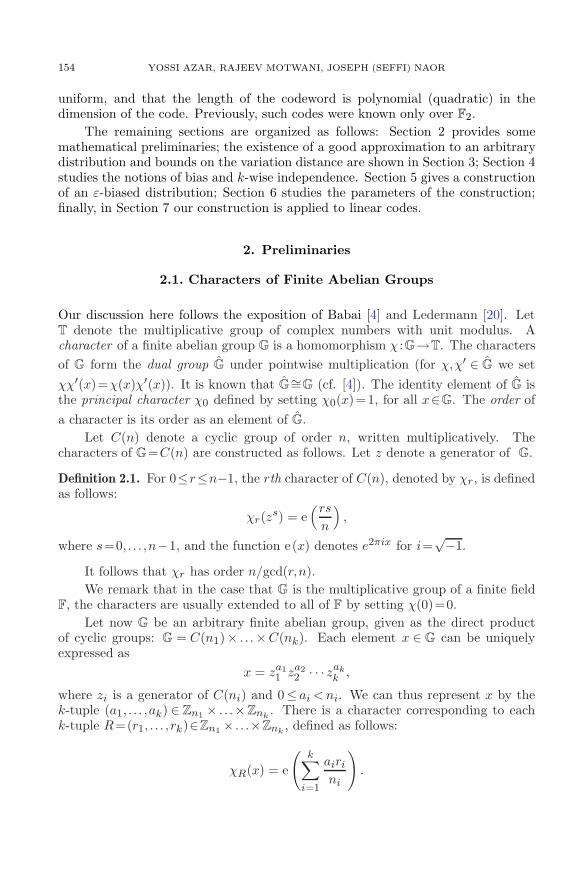
Our discussion here follows the exposition of Babai [4] and Ledermann [20]. LetT denote the multiplicative group of complex numbers with unit modulus. Acharacter of a finite abelian group G is a homomorphism χ :G→T. The charactersof G form the dual group G under pointwise multiplication (for χ,χ′ ∈ G we setχχ′(x)=χ(x)χ′(x)). It is known that G∼=G (cf. [4]). The identity element of G isthe principal character χ0 defined by setting χ0(x)=1, for all x∈G. The order ofa character is its order as an element of G.
Let C(n) denote a cyclic group of order n, written multiplicatively. Thecharacters of G=C(n) are constructed as follows. Let z denote a generator of G.
Definition 2.1. For 0≤r≤n−1, the rth character of C(n), denoted by χr, is definedas follows:
χr(zs) = e(rsn
),
where s=0, . . . ,n−1, and the function e(x) denotes e2πix for i=√−1.
It follows that χr has order n/gcd(r,n).We remark that in the case that G is the multiplicative group of a finite field
F, the characters are usually extended to all of F by setting χ(0)=0.Let now G be an arbitrary finite abelian group, given as the direct product
of cyclic groups: G = C(n1)× . . .×C(nk). Each element x ∈ G can be uniquelyexpressed as
x = za11 za2
2 · · · zakk ,
where zi is a generator of C(ni) and 0≤ ai<ni. We can thus represent x by thek-tuple (a1, . . . ,ak) ∈ Zn1 × . . .×Znk . There is a character corresponding to eachk-tuple R=(r1, . . . ,rk)∈Zn1× . . .×Znk , defined as follows:
χR(x) = e
(k∑i=1
airini
).
APPROXIMATING PROBABILITY DISTRIBUTIONS USING SMALL SAMPLE SPACES 155
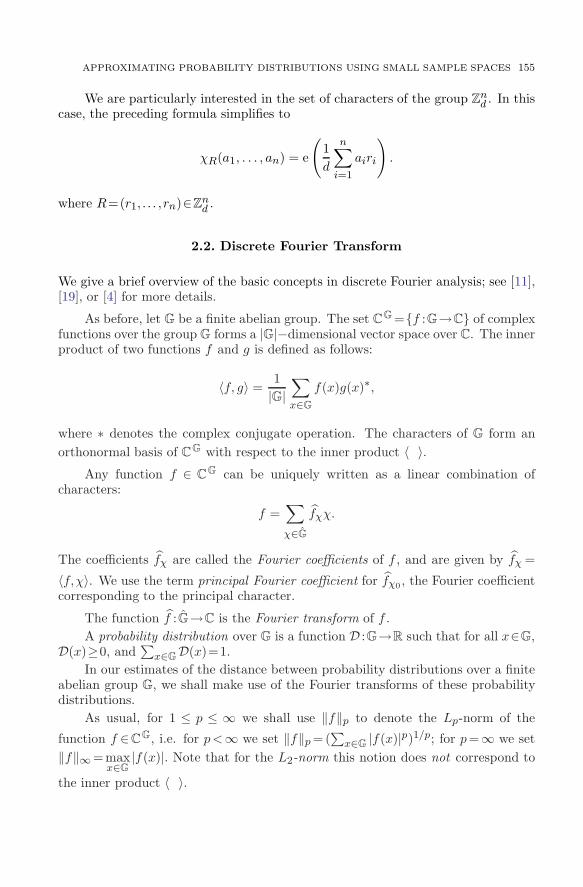
We are particularly interested in the set of characters of the group Znd . In thiscase, the preceding formula simplifies to
χR(a1, . . . , an) = e
(1d
n∑i=1
airi
).
where R=(r1, . . . ,rn)∈Znd .
2.2. Discrete Fourier Transform
We give a brief overview of the basic concepts in discrete Fourier analysis; see [11],[19], or [4] for more details.
As before, let G be a finite abelian group. The set CG=f :G→C of complexfunctions over the groupG forms a |G|−dimensional vector space over C. The innerproduct of two functions f and g is defined as follows:
〈f, g〉 =1|G|
∑x∈G
f(x)g(x)∗,
where ∗ denotes the complex conjugate operation. The characters of G form anorthonormal basis of CG with respect to the inner product 〈 〉.
Any function f ∈ CG can be uniquely written as a linear combination ofcharacters:
f =∑χ∈G
fχχ.
The coefficients fχ are called the Fourier coefficients of f , and are given by fχ =
〈f,χ〉. We use the term principal Fourier coefficient for fχ0 , the Fourier coefficientcorresponding to the principal character.
The function f :G→C is the Fourier transform of f .A probability distribution over G is a function D :G→R such that for all x∈G,
D(x)≥0, and∑x∈GD(x)=1.
In our estimates of the distance between probability distributions over a finiteabelian group G, we shall make use of the Fourier transforms of these probabilitydistributions.
As usual, for 1 ≤ p ≤ ∞ we shall use ‖f‖p to denote the Lp-norm of the
function f ∈CG, i.e. for p<∞ we set ‖f‖p= (∑x∈G |f(x)|p)1/p; for p=∞ we set
‖f‖∞= maxx∈G|f(x)|. Note that for the L2-norm this notion does not correspond to
the inner product 〈 〉.
156 YOSSI AZAR, RAJEEV MOTWANI, JOSEPH (SEFFI) NAOR
3. Approximating arbitrary distributions
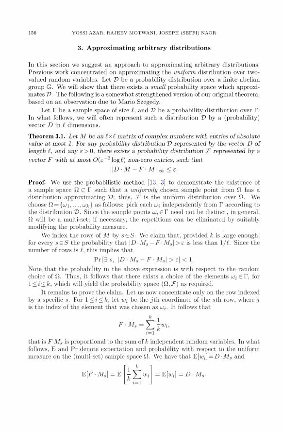
In this section we suggest an approach to approximating arbitrary distributions.Previous work concentrated on approximating the uniform distribution over two-valued random variables. Let D be a probability distribution over a finite abeliangroup G. We will show that there exists a small probability space which approxi-mates D. The following is a somewhat strengthened version of our original theorem,based on an observation due to Mario Szegedy.
Let Γ be a sample space of size `, and D be a probability distribution over Γ.In what follows, we will often represent such a distribution D by a (probability)vector D in ` dimensions.
Theorem 3.1. Let M be an `×` matrix of complex numbers with entries of absolutevalue at most 1. For any probability distribution D represented by the vector D oflength `, and any ε> 0, there exists a probability distribution F represented by a
vector F with at most O(ε−2 log`) non-zero entries, such that
||D ·M − F ·M ||∞ ≤ ε.
Proof. We use the probabilistic method [13, 3] to demonstrate the existence ofa sample space Ω ⊂ Γ such that a uniformly chosen sample point from Ω has adistribution approximating D; thus, F is the uniform distribution over Ω. Wechoose Ω=ω1, . . . ,ωk as follows: pick each ωi independently from Γ according tothe distribution D. Since the sample points ωi∈Γ need not be distinct, in general,Ω will be a multi-set; if necessary, the repetitions can be eliminated by suitablymodifying the probability measure.
We index the rows of M by s∈S. We claim that, provided k is large enough,for every s∈S the probability that |D ·Ms−F ·Ms|>ε is less than 1/`. Since thenumber of rows is `, this implies that
Pr [∃ s, |D ·Ms − F ·Ms| > ε] < 1.Note that the probability in the above expression is with respect to the randomchoice of Ω. Thus, it follows that there exists a choice of the elements ωi ∈Γ, for1≤ i≤k, which will yield the probability space (Ω,F) as required.
It remains to prove the claim. Let us now concentrate only on the row indexedby a specific s. For 1≤ i≤k, let wi be the jth coordinate of the sth row, where jis the index of the element that was chosen as ωi. It follows that
F ·Ms =k∑i=1
1kwi,
that is F ·Ms is proportional to the sum of k independent random variables. In whatfollows, E and Pr denote expectation and probability with respect to the uniformmeasure on the (multi-set) sample space Ω. We have that E[wi]=D ·Ms and
E[F ·Ms] = E
[1k
k∑i=1
wi
]= E[wi] = D ·Ms.
APPROXIMATING PROBABILITY DISTRIBUTIONS USING SMALL SAMPLE SPACES 157
To complete the proof we show that the sum of the wi does not differ fromits expected value by more than εk. Let S be sum of n independent variables,each of which has an absolute value of at most 1. By a version of the Chernoffbound [3, p.240], for any h≥0,
Pr[|S − E[S]| ≥ h] ≤ 2e−Ω(h2/n).
This bound implies that
Pr
[∣∣∣∣∣k∑i=1
wi − kD ·Ms
∣∣∣∣∣ > δ
]≤ 2e−Ω(δ2/k).
In our case, the bound on the allowed deviation from the expected value is δ=εk.We need to choose k such that e−Ω(δ2/k) < 1/2`. This is clearly true for k =Θ(ε−2log `).
The following theorem shows the existence of a good approximation (Ω,F) tothe distribution D such that the sample space Ω is small.
Theorem 3.2. For any probability distribution D defined over a finite abelian groupG and any ε∈ [0,1], there exists a probability space (Ω,F), such that:
1. ‖F −D‖∞≤ε/|G|,2. the size of the probability space Ω is at most O(ε−2log |G|).
Proof. The proof is an immediate consequence of Theorem 3.1. We choose M tobe the character table of the group G, i.e., the rows are indexed by the characters,the columns by the elements of G, and Msx=χs(x).
The following Corollary shows the existence of a good approximation to theuniform distribution over Znd .
Corollary 3.3. There exists a probability distribution F over Znd of sizeO(ε−2n logd)such that the value of all of its Fourier coefficients (except for the principal coeffi-cient) is at most ε/dn.
We now discuss the significance of Theorem 3.2.
Definition 3.4. Let D1 and D2 be two probability distributions over a finite abeliangroup G. We define the variation distance between these two distributions as‖D1−D2‖1.
The next theorem bounds the variation distance between D and F in terms oftheir Fourier coefficients.
Theorem 3.5. Let the probability distributions D and F be defined over a finiteabelian group G. Then,
‖D − F‖1 ≤ |G| · ‖D − F‖2 ≤ |G| · ‖D − F‖1.
158 YOSSI AZAR, RAJEEV MOTWANI, JOSEPH (SEFFI) NAOR
Proof. The right inequality is immediate. Let H = D−F . Using the Cauchy–Schwarz Inequality and Parseval’s Equality, we conclude that
‖H‖1 ≤√|G| · ‖H‖2 = |G| · ‖H‖2.
Let X1, . . . ,Xn be random variables taking values from Zd. Let D : Znd → Rdenote their joint probability distribution. Let S ⊆ 1, . . .n be of cardinality k.For any x∈ Znd , let x|S denote the projection of the vector x specified by S. Wedefine DS , the restriction of D to S, by setting
DS(XS = y) =∑
x∈Znd,x|S=y
D(x)
for all y∈Zkd.We first observe the following relation between the Fourier coefficients of D
and DS . Let A⊂Znd denote the set of elements (a1, . . . ,an) in Znd for which ai=0for all i 6∈S.
Lemma 3.6. For all A∈A,
dn−k · u = v
where u is the Fourier coefficient of D corresponding to A, and v is the Fouriercoefficient of DS corresponding to A|S .
Proof. The proof follows directly by substituting appropriate values into thedefinition of Fourier coefficients.
Corollary 3.7. Let D and F be probability distributions defined over Znd such that
‖D−F‖∞≤ε/dn for some 0≤ε≤1. Then, for any subset S of cardinality k of therandom variables,
‖DS −FS‖1 ≤ εdk.
Proof. Applying Theorem 3.5 and Lemma 3.6, we conclude that
‖DS −FS‖1 ≤ dk · ‖DS − FS‖1≤ d2k · ‖DS − FS‖∞≤ d2k · dn−k · ‖D − F‖∞
≤ dn+k · εdn
= εdk,
which completes the proof.
If ε is chosen to be polynomially small, then Corollary 3.7 implies that: for anydistribution D, there exists a distribution F over a polynomial size sample spacesuch that any subset S of the random variables is distributed in F “almost” as inD, provided that |S|=O(logdn).

APPROXIMATING PROBABILITY DISTRIBUTIONS USING SMALL SAMPLE SPACES 159
4. Bias and k-wise near-independence
In this section we define the notion of a ε-biased distribution. (This distribution hasbeen studied earlier [25, 1] for the case d= 2). Generalized ε-biased distributionsrepresent a convenient formalization of the concept of “good” approximation tothe uniform distribution. Our main result here is a theorem that bounds theFourier coefficients of a probability distribution over Znd in terms of the bias ofthe distribution. We also give a bound on the variation distance of a distributionfrom the uniform distribution in terms of the Fourier coefficients.
We first generalize the definition of ε-biased distributions to the case of multi-valued random variables. Let X = (X1, . . . ,Xn) be a random variable over a setΩ⊆Znd . We define the bias of X with respect to any A∈Znd as follows.
Definition 4.1. Let A=(a1, . . . ,an) be any vector in Znd and let g=gcd(a1, . . . ,an,d).The bias of A is defined to be
bias (A) =1g
max0≤k< d
g
∣∣∣∣∣Pr
[n∑i=1
aiXi ≡ kg (mod d)
]− g
d
∣∣∣∣∣ .We introduce g in this definition because, regardless of the distribution of the
random variables, the only values that∑ni=1aiXi (mod d) can take are multiples
of g.
Definition 4.2. Let 0≤ε≤1 and let Ω⊆Znd . A probability space (Ω,P) is said to beε-biased if the corresponding random variable X = (X1, . . . ,Xn) has the followingproperties.
1. For 1≤ i≤n, Xi is uniformly distributed over Zd.2. For all vectors A∈Znd , bias(A)≤ε.
We first note that Theorem 3.1 implies that an ε-biased probability space ofsmall size exists. In Section 5 we provide an explicit construction which is somewhatweaker.
Corollary 4.3. There exists a probability distribution F over Znd of sizeO(ε−2n logd)such that for all A=(a1, . . . ,an)∈Znd , bias(A)≤ε.
Proof. The proof follows immediately from Theorem 3.1 by the following choice ofmatrix M . Let the columns of M correspond to the elements of Znd , and the rowsof M correspond to all pairs (A,k) such that A = (a1, . . . ,an) ∈ Znd , 0 ≤ k < d/g,where g=gcd(a1, . . . ,an,d). Let X=(X1, . . . ,Xn)∈Znd . We define:
M((A, k), X) =
1 if
n∑i=1
aiXi ≡ kg (mod d)
0 otherwise.
160 YOSSI AZAR, RAJEEV MOTWANI, JOSEPH (SEFFI) NAOR
In order to apply Theorem 3.1, we transform matrix M into a square matrix byadding zero rows.
Let D be an ε-biased distribution. We now relate the bias and the Fouriercoefficient for any A∈Znd as follows.
Lemma 4.4. For all non-zero A=(a1, . . . ,an)∈Znd , we have that
|DA| ≤bias (A)dn−1
.
Proof. Let g=gcd(a1, . . . ,an,d). By the definition of a Fourier coefficient,
DA = 〈D, χA〉
=1dn
∑x
D(x)χA(x)∗
=1dn
∑x
D(x)
(e
(1d
n∑i=1
aixi
))∗
=1dn
∑x
D(x)e
(−1d
n∑i=1
aixi
).
Taking absolute values, we have that
|DA| =1dn
∣∣∣∣∣∑x
D(x)e(−1d
∑aixi
)∣∣∣∣∣=
1dn
∣∣∣∣∣∣∣dg−1∑k=0
e(−kgd
)Pr[∑
aixi ≡ kg (mod d)]∣∣∣∣∣∣∣ .
The probability is with respect to a random choice of x∈Znd with the distributionD. Define Pkg=Pr[
∑aixi≡kg (mod d)]. Then,
|DA| =1dn
∣∣∣∣∣∣∣dg−1∑k=0
e(−kgd
)Pkg
∣∣∣∣∣∣∣=
1dn
∣∣∣∣∣∣∣g
d
dg−1∑k=0
e(−kgd
)+
dg−1∑k=0
e(−kgd
)(Pkg −
g
d
)∣∣∣∣∣∣∣

APPROXIMATING PROBABILITY DISTRIBUTIONS USING SMALL SAMPLE SPACES 161
Note that∑
e(−kgd
)= 0 since the (d/g)th roots of unity sum to zero. We then
conclude that
|DA| =1dn
∣∣∣∣∣∣∣dg−1∑k=0
e(−kgd
)(Pkg −
g
d
)∣∣∣∣∣∣∣≤ 1dn
dg−1∑k=0
∣∣∣∣e(−kgd)∣∣∣∣ ∣∣∣Pkg − g
d
∣∣∣≤ 1dn· dg· (g · bias (A))
=bias (A)dn−1
,
where the last inequality follows from the definition of the bias as well as the factthat |e(−kg/d)|=1.
The following theorem is a generalization of a result due to Vazirani [28]. Itrelates the biases of an arbitrary distribution to its variation distance from theuniform distribution.
Theorem 4.5. Let D be an arbitrary probability distribution defined on Znd , and let
U denote the uniform distribution on Znd . Then,
||D − U||1 ≤ d∑A
bias (A),
where the bias is defined with respect to the distribution D.
Proof. We first evaluate D~0,
D(~0) = 〈D, χ~0〉 =∑x∈Zdn
D(x)dn
=1dn.
The variation distance is,
||D − U||1 =∑x∈Zdn
∣∣∣∣D(x) − 1dn
∣∣∣∣ =∑x∈Zdn
∣∣∣∣∣∑A
DAχA(x) − 1dn
∣∣∣∣∣ .
162 YOSSI AZAR, RAJEEV MOTWANI, JOSEPH (SEFFI) NAOR
Since D~0 = 1dn ,
∑x∈Zdn
∣∣∣∣∣∑A
DAχA(x)− 1dn
∣∣∣∣∣ =∑x∈Zdn
∣∣∣∣∣∣∑A 6=~0
DAχA(x)
∣∣∣∣∣∣≤∑x∈Zdn
∑A 6=~0
∣∣∣DA∣∣∣ |χA(x)|
= dn∑A 6=~0
∣∣∣DA∣∣∣≤ dn
∑A
d
dnbias (A),
where the last inequality follows from Lemma 4.4. Thus,
||D − U||1 ≤ d∑A 6=~0
bias (A).
Corollary 4.6. For ε = 0, an ε-biased distribution is the same as the uniformdistribution.
The following definition is similar to that of Naor and Naor [25] and Ben-Nathan [6].
Definition 4.7. Let X1, . . . ,Xn be random variables taking values from Zd. LetD : Znd → R denote their joint probability distribution. For any x ∈ Znd , let x|Sdenote the projection of the vector x specified by S. Let DS denote the restrictionof D to S, by setting
DS(XS = y) =∑
x∈Znd,x|S=y
D(x)
for all y∈Zkd . We say that the variables X1, . . ., Xn are k-wise δ-dependent if forall subsets S such that |S|≤k,
||D(S)− U(S)||1 ≤ δ,
where U denotes the uniform distribution.
The next Corollary follows from Theorem 4.5 and Corollary 3.7.
Corollary 4.8. If the random variables X1, . . . ,Xn taking values from Zd are ε-
biased, then they are also k-wise δ-dependent, for δ= εdk. In particular, they are(logdn)-wise (1/poly(n))-dependent with a polynomially small ε.
APPROXIMATING PROBABILITY DISTRIBUTIONS USING SMALL SAMPLE SPACES 163
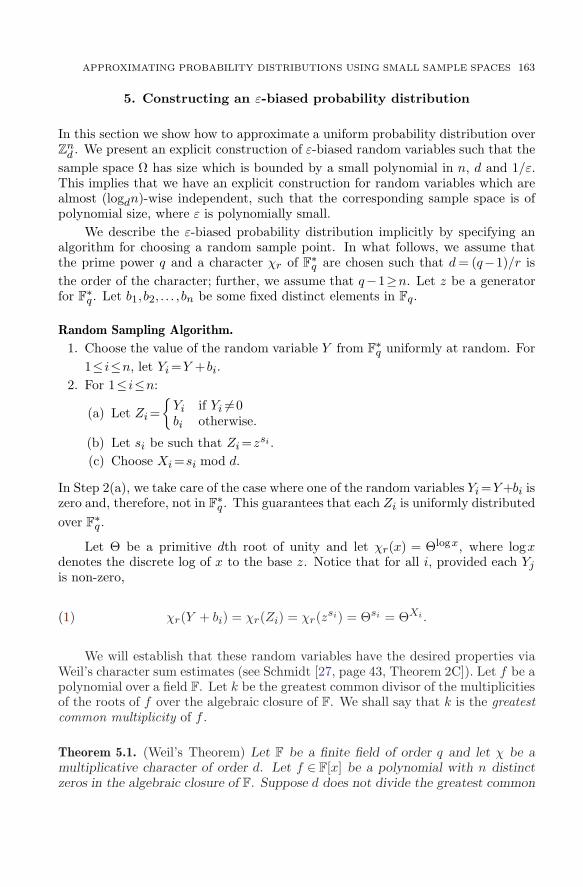
5. Constructing an ε-biased probability distribution
In this section we show how to approximate a uniform probability distribution overZnd . We present an explicit construction of ε-biased random variables such that thesample space Ω has size which is bounded by a small polynomial in n, d and 1/ε.This implies that we have an explicit construction for random variables which arealmost (logdn)-wise independent, such that the corresponding sample space is ofpolynomial size, where ε is polynomially small.
We describe the ε-biased probability distribution implicitly by specifying analgorithm for choosing a random sample point. In what follows, we assume thatthe prime power q and a character χr of F∗q are chosen such that d= (q−1)/r isthe order of the character; further, we assume that q−1≥n. Let z be a generatorfor F∗q . Let b1, b2, . . . , bn be some fixed distinct elements in Fq.
Random Sampling Algorithm.
1. Choose the value of the random variable Y from F∗q uniformly at random. For1≤ i≤n, let Yi=Y +bi.
2. For 1≤ i≤n:
(a) Let Zi=Yi if Yi 6=0bi otherwise.
(b) Let si be such that Zi=zsi .(c) Choose Xi=si mod d.
In Step 2(a), we take care of the case where one of the random variables Yi=Y+bi iszero and, therefore, not in F∗q . This guarantees that each Zi is uniformly distributedover F∗q .
Let Θ be a primitive dth root of unity and let χr(x) = Θlogx, where logxdenotes the discrete log of x to the base z. Notice that for all i, provided each Yjis non-zero,
(1) χr(Y + bi) = χr(Zi) = χr(zsi) = Θsi = ΘXi .
We will establish that these random variables have the desired properties viaWeil’s character sum estimates (see Schmidt [27, page 43, Theorem 2C]). Let f be apolynomial over a field F. Let k be the greatest common divisor of the multiplicitiesof the roots of f over the algebraic closure of F. We shall say that k is the greatestcommon multiplicity of f .
Theorem 5.1. (Weil’s Theorem) Let F be a finite field of order q and let χ be amultiplicative character of order d. Let f ∈ F[x] be a polynomial with n distinctzeros in the algebraic closure of F. Suppose d does not divide the greatest common

164 YOSSI AZAR, RAJEEV MOTWANI, JOSEPH (SEFFI) NAOR
multiplicity of f . Then ∣∣∣∣∣∣∑x∈F
χ(f(x))
∣∣∣∣∣∣ ≤ (n− 1)√q.
To analyze the properties of our construction, we need the following corollary.
Corollary 5.2. Let F be a finite field of order q and let Θ be a primitive dth rootof unity. Let f ∈F[x] be a polynomial with n distinct roots in the algebraic closureof F. Assume that the greatest common multiplicity of f is relatively prime to d.
Define rk to be the number of solutions x∈F to the equation χ(f(x))=Θk. Then,∣∣∣rk − q
d
∣∣∣ ≤ (n− 1)√q.
Proof. The definition of rj implies that for 0≤`≤d−1,
(2)∑x∈F
(χ(f(x)))` =d−1∑j=0
rjΘ`j .
(Here for `=0 we set 0`=0.) Denoting the number of distinct roots of f in F by ν(ν≤n), it follows that
q − ν +d−1∑`=1
∑x∈F
(χ(f(x)))` =d−1∑`=0
∑x∈F
(χ(f(x)))`
=d−1∑`=0
d−1∑j=0
rjΘ`j
= dr0 +d−1∑j=1
rj
d−1∑`=0
Θj`
= dr0.
Hence,
|dr0 − q| ≤ ν +
∣∣∣∣∣∣d−1∑`=1
∑x∈F
(χ(f(x)))`
∣∣∣∣∣∣ ≤ ν +d−1∑`=1
∣∣∣∣∣∣∑x∈F
(χ(f(x)))`
∣∣∣∣∣∣ .The order of the character χ` is d′=d/gcd(d,`) which is greater than 1 for 0<`<dand it is relatively prime to the greatest common multiplicity of f , hence we mayapply Theorem 5.1 to each term on the right hand side. We obtain
|dr0 − q| ≤ ν +d−1∑`=1
(n− 1)√q ≤ ν + (d− 1)(n− 1)
√q < d(n− 1)
√q.
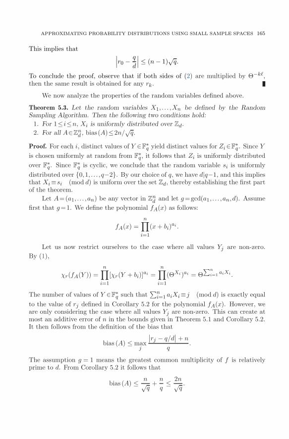
APPROXIMATING PROBABILITY DISTRIBUTIONS USING SMALL SAMPLE SPACES 165
This implies that ∣∣∣r0 − q
d
∣∣∣ ≤ (n− 1)√q.
To conclude the proof, observe that if both sides of (2) are multiplied by Θ−k`,then the same result is obtained for any rk.
We now analyze the properties of the random variables defined above.
Theorem 5.3. Let the random variables X1, . . . ,Xn be defined by the RandomSampling Algorithm. Then the following two conditions hold:
1. For 1≤ i≤n, Xi is uniformly distributed over Zd.2. For all A∈Znd , bias(A)≤2n/
√q.
Proof. For each i, distinct values of Y ∈F∗q yield distinct values for Zi∈F∗q . Since Yis chosen uniformly at random from F∗q , it follows that Zi is uniformly distributedover F∗q . Since F∗q is cyclic, we conclude that the random variable si is uniformlydistributed over 0,1, . . . ,q−2. By our choice of q, we have d|q−1, and this impliesthat Xi≡si (mod d) is uniform over the set Zd, thereby establishing the first partof the theorem.
Let A=(a1, . . . ,an) be any vector in Znd and let g=gcd(a1, . . . ,an,d). Assumefirst that g=1. We define the polynomial fA(x) as follows:
fA(x) =n∏i=1
(x+ bi)ai .
Let us now restrict ourselves to the case where all values Yj are non-zero.By (1),
χr(fA(Y )) =n∏i=1
[χr(Y + bi)]ai =n∏i=1
(ΘXi)ai = Θ∑n
i=1aiXi .
The number of values of Y ∈F∗q such that∑ni=1 aiXi≡j (mod d) is exactly equal
to the value of rj defined in Corollary 5.2 for the polynomial fA(x). However, weare only considering the case where all values Yj are non-zero. This can create atmost an additive error of n in the bounds given in Theorem 5.1 and Corollary 5.2.It then follows from the definition of the bias that
bias (A) ≤ maxj
∣∣rj − q/d∣∣+ n
q.
The assumption g = 1 means the greatest common multiplicity of f is relativelyprime to d. From Corollary 5.2 it follows that
bias (A) ≤ n√q
+n
q≤ 2n√q.

166 YOSSI AZAR, RAJEEV MOTWANI, JOSEPH (SEFFI) NAOR
Consider now the case g > 1, and let βi = ai/g. Let g′ = gcd(a1, . . . ,an) andci = ai/g
′. By the preceding argument, the bias of the vector C = (c1, . . . , cn) isbounded by 2n/
√q. For 0≤ j≤ d/g−1, the number of vectors X that satisfy the
equationn∑i=1
aiXi ≡ jg (mod d).
is equal to the number of vectors X that satisfy
n∑i=1
ciXi ≡ j +dl
g(mod d),
where 0≤ l≤g−1. Since g′/g is relatively prime to d/g, the number of such vectorsis also equal to the number of vectors X that satisfy
n∑i=1
ciXi ≡ j′ +dl′
g(mod d)
where j≡j′(g′/g) (mod d/g). By Definition 4.3,
bias (A) =1d· d · bias (G) = bias (G),
which establishes the second part of the theorem.
The parameters of our construction are described in the following theorem.Let q(d,k) denote the smallest prime power such that d|q−1 and d≥k.
Theorem 5.4. For any ε>0, n≥2, and d≥2, the probability space (Ω,P) definedby the Random Sampling Algorithm generates n random variables over Zd which
are ε-biased, and the size of the sample space is |Ω|=q(d,4n2ε−2)−1.
Proof. Generating the random variables X only requires choosing Y ∈F∗q uniformlyat random. Hence the sample space is Ω=F∗q where q is a prime such that d|q−1
and q≥4n2ε−2. Choose the smallest prime power satisfying these constraints.
6. Estimates for q(d,k)
In this section we review results from number theory relevant to estimating q(d,k).Let p(d,k) denote the smallest prime such that d|p−1 and d≥k. Clearly q(d,k)≤p(d,k).
For any d and k, the quantity p(d,k) can be estimated using Linnik’s Theoremestablishing the existence of small primes in arithmetic progressions: among the

APPROXIMATING PROBABILITY DISTRIBUTIONS USING SMALL SAMPLE SPACES 167
integers ≡ t (modm) (where gcd(m,t) = 1) there exists a prime p = O(mC ).Heath-Brown [17] proves C ≤ 11/2. Note that this result does not depend on anyhypothesis. Under the Extended Riemann Hypothesis, Bach and Sorenson [5] provethat p can be chosen to be ≤2(m lnm)2, hence C≤2+o(1).
Let now p(d) denote the smallest prime such that d|p−1. Let further m(d,k)be the smallest integer m such that d|m and m≥k. Note that m(d,k)<d+k. Notefurther that p(d,k)≤p(m(d,k)). Summarizing, there exist absolute constants c andC such that
(3) p(d, k) < c(d+ k)C .
Here C is the exponent in Linnik’s Theorem discussed above.The exponent C can be reduced to 1 if d is small compared to k. For fixed d
we have
(4) p(d, k) < (1 + o(1))k.
Moreover, for any constant c>0 and for any d≤ logc k we have
(5) p(d, k) < c1k,
where the constant c1 depends only on c. These bounds follow from results that inthis range, the primes are nearly uniformly distributed among the mod d residueclasses which are relatively prime to d (prime number theorem for arithmeticprogressions, cf. [10, pp. 132-133]).
In conclusion we summarize the bounds obtained for the size of the samplespace.
Theorem 6.1. For any ε > 0, n ≥ 2, and d ≥ 2, the probability space (Ω,P)defined by the Random Sampling Algorithm generates n random variables over
Zd which are ε-biased, and the size of the sample space is |Ω| < c0(d+n2ε−2)C
where C is the constant in Linnik’s Theorem. Moreover, if d≤ logc(n2ε−2) then
we have |Ω| < c1n2ε−2 where c1 depends on c only. For constant d we have
|Ω|<(1+o(1))n2ε−2.
Note that the bounds obtained in the above theorem are not the best possible,compare with Corollary 4.3. Theorem 6.1 together with Corollary 4.8 imply that wecan construct (logdn)-wise (1/poly(n))-dependent random variables over Znd using apolynomially large sample space. Also, Theorem 6.1 together with Lemma 4.4 implythat we can approximate the Fourier coefficients of the uniform distribution on Zndwithin ε/dn with a sample space of size O(ε−2n2d2) for small d. This constructionmay not be the best possible since Corollary 3.3 guarantees the existence of anapproximating sample space whose size is O(ε−2n logd).
168 YOSSI AZAR, RAJEEV MOTWANI, JOSEPH (SEFFI) NAOR
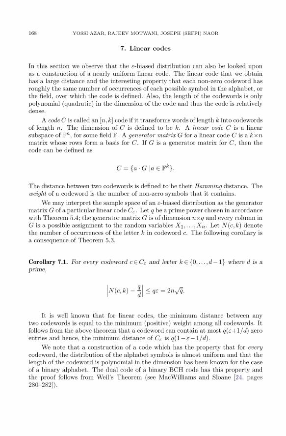
7. Linear codes
In this section we observe that the ε-biased distribution can also be looked uponas a construction of a nearly uniform linear code. The linear code that we obtainhas a large distance and the interesting property that each non-zero codeword hasroughly the same number of occurrences of each possible symbol in the alphabet, orthe field, over which the code is defined. Also, the length of the codewords is onlypolynomial (quadratic) in the dimension of the code and thus the code is relativelydense.
A code C is called an [n,k] code if it transforms words of length k into codewordsof length n. The dimension of C is defined to be k. A linear code C is a linearsubspace of Fn, for some field F. A generator matrix G for a linear code C is a k×nmatrix whose rows form a basis for C. If G is a generator matrix for C, then thecode can be defined as
C = a ·G |a ∈ Fk.
The distance between two codewords is defined to be their Hamming distance. Theweight of a codeword is the number of non-zero symbols that it contains.
We may interpret the sample space of an ε-biased distribution as the generatormatrixG of a particular linear code Cε. Let q be a prime power chosen in accordancewith Theorem 5.4; the generator matrix G is of dimension n×q and every column inG is a possible assignment to the random variables X1, . . . ,Xn. Let N(c,k) denotethe number of occurrences of the letter k in codeword c. The following corollary isa consequence of Theorem 5.3.
Corollary 7.1. For every codeword c∈Cε and letter k ∈0, . . . ,d−1 where d is aprime,
∣∣∣N(c, k)− q
d
∣∣∣ ≤ qε = 2n√q.
It is well known that for linear codes, the minimum distance between anytwo codewords is equal to the minimum (positive) weight among all codewords. Itfollows from the above theorem that a codeword can contain at most q(ε+1/d) zeroentries and hence, the minimum distance of Cε is q(1−ε−1/d).
We note that a construction of a code which has the property that for everycodeword, the distribution of the alphabet symbols is almost uniform and that thelength of the codeword is polynomial in the dimension has been known for the caseof a binary alphabet. The dual code of a binary BCH code has this property andthe proof follows from Weil’s Theorem (see MacWilliams and Sloane [24, pages280–282]).
APPROXIMATING PROBABILITY DISTRIBUTIONS USING SMALL SAMPLE SPACES 169
8. Open Problems
An important direction for further work is to efficiently construct (in time polyno-mial in the number of random variables n) probability distributions that approx-imate special types of joint distributions. In particular, can we construct in timepolynomial in n a good approximation to the joint distribution where each randomvariable independently takes value 1 with probability p and 0 with probability 1−p?Note that this is only known for the case where p=1/2.
It is also not clear that our construction of an ε-biased distribution on n d-valued random variables is the best possible. Theorem 3.2 guarantees the existenceof such a distribution using a smaller sample space (by a factor of n). Can this beachieved constructively?
Acknowledgements. The authors would like to thank Noga Alon and Moni Naor forseveral helpful discussions. We are also grateful to Laci Babai for simplifying theproof of Corollary 5.2 and to Mario Szegedy for his remarks concerning Theorem3.1. Special thanks go to the anonymous referees and the editor Laci Babai forefforts above and beyond the call of duty towards improving the quality of thisarticle.
References
[1] N. Alon, O. Goldreich, J. Hastad, and R. Peralta: Simple Constructions of
Almost k-wise Independent Random Variables, Random Structures and Algo-
rithms, 3 (1992), 289–304.
[2] N. Alon, L. Babai, and A. Itai: A fast and simple randomized parallel algorithm
for the maximal independent set problem, Journal of Algorithms, 7 (1986), 567–
583.
[3] N. Alon and J. Spencer: The Probabilistic Method, John Wiley, 1992.
[4] L. Babai: Fourier Transforms and Equations over Finite Abelian Groups, Lecture
Notes, University of Chicago, 1989.
[5] E. Bach and J. Sorenson: Explicit Bounds for Primes in Residue Classes, Mathe-
matics of Computation, 65 (1996), 1717–1735.
[6] R. Ben-Nathan: On dependent random variables over small sample spaces,
M.Sc. Thesis, Hebrew University, Jerusalem, Israel (1990).
[7] B. Berger and J. Rompel: Simulating (logcn)-wise independence in NC, Journal
of the ACM, 38 (1991), 1026–1046.
[8] B. Chor and O. Goldreich: On the power of two-point based sampling, Journal
of Complexity, 5 (1989), 96–106.
[9] B. Chor, O. Goldreich, J. Hastad, J. Friedman, S. Rudich, and R. Smolen-
sky: t-Resilient functions, In Proceedings of the 26th Annual Symposium on the
Foundations of Computer Science (1985), 396–407.
[10] H. Davenport: Multiplicative Number Theory, 2nd Edition, Springer Verlag, 1980.
170 YOSSI AZAR, RAJEEV MOTWANI, JOSEPH (SEFFI) NAOR
[11] H. Dym and H. P. McKean: Fourier Series and Integrals, Academic Press, 1972.
[12] P. Erdos and J. Selfridge: On a combinatorial game, J. Combinatorial Theory,
Ser. B, 14 (1973), 298–301.
[13] P. Erdos and J. Spencer: Probabilistic Methods in Combinatorics, Akademiai
Kiado, Budapest, 1974.
[14] T. Estermann: Introduction to Modern Prime Number Theory, Cambridge Univer-
sity Press, 1969.
[15] G. Even: Construction of small probability spaces for deterministic simulation,
M.Sc. Thesis, Technion, Haifa, Israel (1991).
[16] J. Hastad, S. Phillips, and S. Safra: A Well Characterized Approximation
Problem, In Proceedings of the 2nd Israel Symposium on Theory and Computing
Systems (1993), 261–265.
[17] D. R. Heath-Brown: Zero-Free Regions for Dirichlet L-Functions and the Least
Prime in an Arithmetic Progression, Proc. London Math. Soc. 64 (1991), 265–
338.
[18] R. M. Karp and A. Wigderson: A Fast Parallel Algorithm for the Maximal
Independent Set Problem, Journal of the ACM, 32 (1985), 762–773.
[19] T. W. Korner: Fourier Analysis, Cambridge University Press (1988).
[20] W. Ledermann: Introduction to Group Characters, Cambridge University Press
(1987, 2nd edition).
[21] M. Luby: A simple parallel algorithm for the maximal independent set, SIAM
Journal on Computing, 15 (1986), 1036–1053.
[22] M. Luby: Removing randomness in parallel computation without a processor
penalty, In Proceedings of the 29th Annual Symposium on Foundations of Com-
puter Science (1988), 162–173.
[23] R. Motwani, J. Naor, and M. Naor: The probabilistic method yields deterministic
parallel algorithms, Journal of Computer and System Sciences, 49 (1994), 478-
516.
[24] F. J. MacWilliams and N. J. A. Sloane: The Theory of Error Correcting Codes,
North-Holland (1977).
[25] J. Naor and M. Naor: Small-bias probability spaces: efficient constructions and
applications, SIAM Journal on Computing, 22 (1993), 838–856.
[26] R. Peralta: On the randomness complexity of algorithms, CS Research Report TR
90-1, University of Wisconsin, Milwaukee (1990).
[27] W. M. Schmidt: Equations over Finite Fields: An Elementary Approach, Lecture
Notes in Mathematics, v. 536, Springer-Verlag (1976).
APPROXIMATING PROBABILITY DISTRIBUTIONS USING SMALL SAMPLE SPACES 171
[28] U. Vazirani: Randomness, Adversaries and Computation, Ph.D. Thesis, University
of California, Berkeley (1986).
Yossi Azar
Computer Science Department
Tel Aviv University
Tel Aviv 69978, Israel
Rajeev Motwani
Computer Science Department
Stanford University
Stanford, CA 94305
Joseph (Seffi) Naor
Computer Science Department
Technion
Haifa 32000, Israel