Embed Size (px)
Citation preview

Approximating Minimum Power Degree and Connectivity Problems
Zeev NutovThe Open University of Israel
Joint Work with: Guy Kortsarz
Vahab Mirrokni
Elena Tsanko

2
Talk Outline
• Min-Power Problems - Motivation • Defining the Problems • Relations Between the Problems• Our Results• O(log n)-Approximation Algorithm for
Min-Power Edge-Multi-Cover (MPEMC)• 3/2-Approximation Algorithm for
Min-Power Edge-Cover (MPEC)

3
The Cost Measure-Wired Networks:connecting every two nodes incurs a cost.
• Nodes in the network correspond to transmitters.
• More power larger transmission range.
• Transmission range = usually (but not always)
disk centered at the node.
The Power Measure-Wireless Networks:every node connects to all nodes in its “range”.
The Power Measure-Motivation
Goal: Find min-power range assignment so that
the resulting communication network satisfies
some prescribed property.
4
b
a
c
d
g
f
e
a
b
d
g
f
e
c
Range assignment Communication network
Example
5
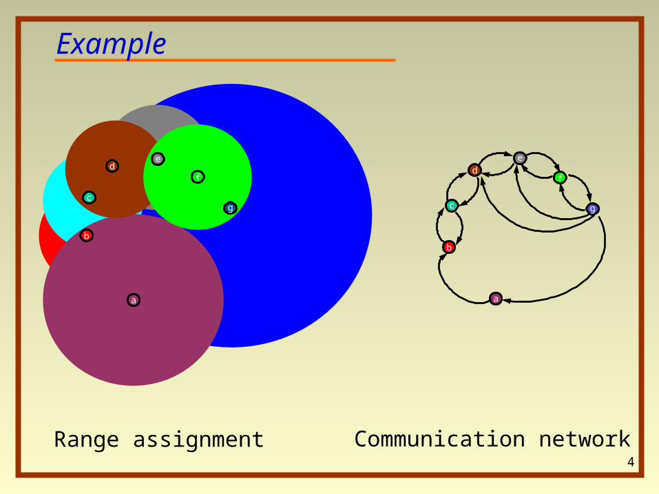
Relating powers and costs:
Directed: c(H)/Δ(H) ≤ p(H) ≤ c(H) (Δ(H)=max-outdegree)
Undirected: c(H)/√|F|/2 ≤ p(H) ≤ 2c(H)
c(H) ≤ p(H) ≤ 2c(H) if H is a forest
c(H) = n-1
p(H) = n
c(H) = n-1
p(H) = 1
directed undirected
Power vs Cost
Definition: Let H=(V,F) be a graph with edge-costs {c(e):eF}power of v in H: pF(v) = max{c(e):eF(v)} = maximum cost of an edge leaving vThe power of H: p(H) = pF(V)= ∑vV pF(v)
−−−
6
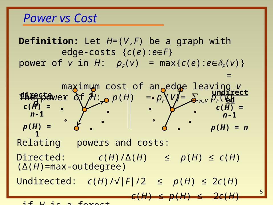
Minimum Power Edge-Multi-Cover (MPEMC)Instance: A graph G = (V,E) with edge costs {c(e):e E}, and degree requirements {r(v):v V}.
Objective: Find a minimum power subgraph H of G so that H is an r-edge-cover.
Defining the ProblemsDefinition: Given a degree requirement function r on V, an edge set F on V is an r-edge-cover if degF(v) ≥ r(v) for all v V
Minimum Power k-Connected Subgraph (MPkCS)Instance: A graph G = (V,E) with edge costs {c(e):e E}, and an integer k. Objective: Find a minimum power k-connected spanning
subgraph H of G.
7
k-1k-clique
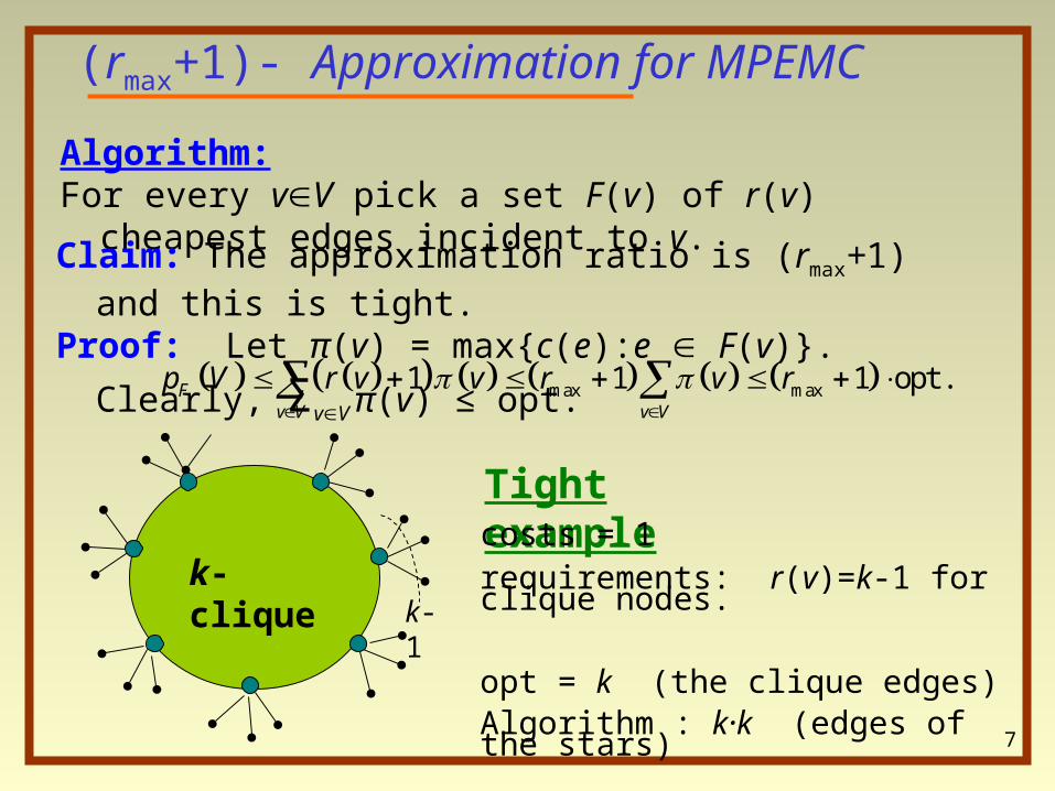
(rmax+1)- Approximation for
MPEMC Algorithm: For every vV pick a set F(v) of r(v) cheapest edges incident to v.
Tight examplecosts = 1requirements: r(v)=k-1 for clique nodes.
opt = k (the clique edges)Algorithm : k·k (edges of the stars)
max max1 1 1 opt .Fv V v V
p V r v v r v r
Claim: The approximation ratio is (rmax+1) and this is tight.
Proof: Let π(v) = max{c(e):e F(v)}. Clearly, ΣvV π(v) ≤ opt.
8
Relating Approximation Ratios
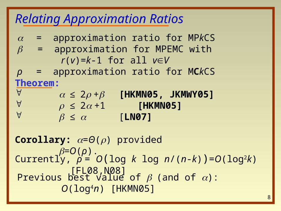
= approximation ratio for MPkCS = approximation for MPEMC with r(v)=k-1 for all vV ρ = approximation ratio for MCkCS
Currently, ρ = O(log k log n/(n-k))=O(log2k) [FL08,N08]
Corollary: =Θ() provided =O(ρ).
Theorem: ≤ 2 + [HKMN05, JKMWY05] ≤ 2 +1 [HKMN05] ≤ [LN07]
Previous best value of (and of ): O(log4n) [HKMN05]

9
Our Result
Theorem 1MPEMC admits an O(log n)-approximation algorithm.Thus MPkCS admits an approximation algorithm with ratio O(log n + log k log n/(n-k)) = O(log n log n/(n-k)).
Previous ratio for MPEMC, MPkCS: O(log4n) [HKMN05].
What about MPEC, when we have 0,1 requirements?
Previous ratio for MPEC: 2.
Theorem 2MPEC admits a 3/2-approximation algorithm.
10
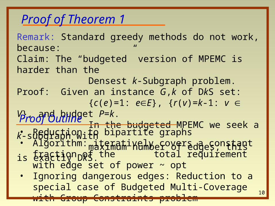
Proof of Theorem 1
• Reduction to bipartite graphs • Algorithm: iteratively covers a constant fraction of the
total requirement with edge set of power ~ opt• Ignoring dangerous edges: Reduction to a special case of
Budgeted Multi-Coverage with Group Constraints problem
Remark: Standard greedy methods do not work, because:Claim: The “budgeted” version of MPEMC is harder than the Densest k-Subgraph problem.Proof: Given an instance G,k of DkS set: {c(e)=1: eE}, {r(v)=k-1: v V}, and budget P=k. In the budgeted MPEMC we seek a k-subgraph with maximum number of edges; this is exactly DkS.
Proof Outline
11
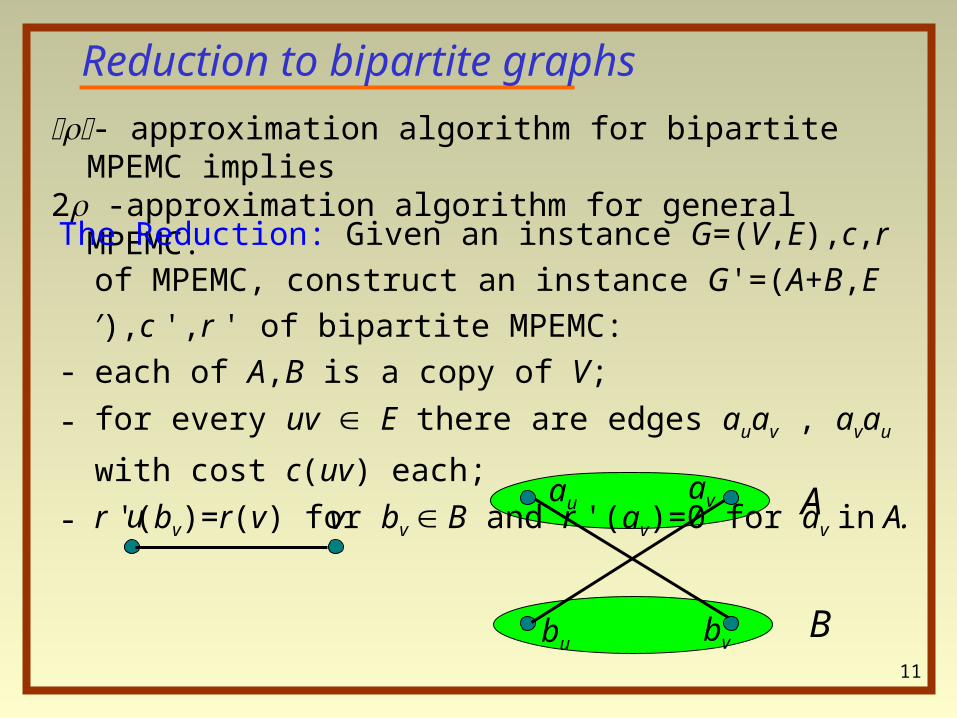
Reduction to bipartite graphs
- approximation algorithm for bipartite MPEMC implies2 -approximation algorithm for general MPEMC.
auav
bvbu
A
B
u v
The Reduction: Given an instance G=(V,E),c,r of MPEMC,
construct an instance G'=(A+B,E′),c ',r ' of bipartite MPEMC:- each of A,B is a copy of V;
- for every uv E there are edges auav , avau with cost c(uv) each;
- r '(bv)=r(v) for bv B and r '(av)=0 for av in A.
12
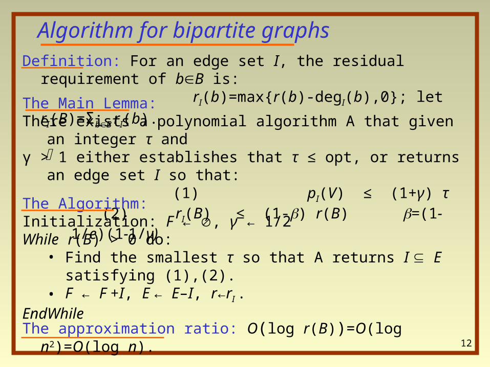
Algorithm for bipartite graphs
The Main Lemma: There exists a polynomial algorithm A that given an integer τ andγ > 1 either establishes that τ ≤ opt, or returns an edge set I so that:
(1) pI(V) ≤ (1+γ) τ (2) rI(B) ≤ (1-) r(B) =(1-1/e)(1-1/γ)
Definition: For an edge set I, the residual requirement of bB is: rI(b)=max{r(b)-degI(b),0}; let rI(B)=ΣbB rI(b).
The Algorithm: Initialization: F ← , γ ← 1/2While r(B) > 0 do:
• Find the smallest τ so that A returns I E satisfying (1),(2).• F ← F +I, E ← E–I, r←rI .
EndWhile
The approximation ratio: O(log r(B))=O(log n2)=O(log n).
13
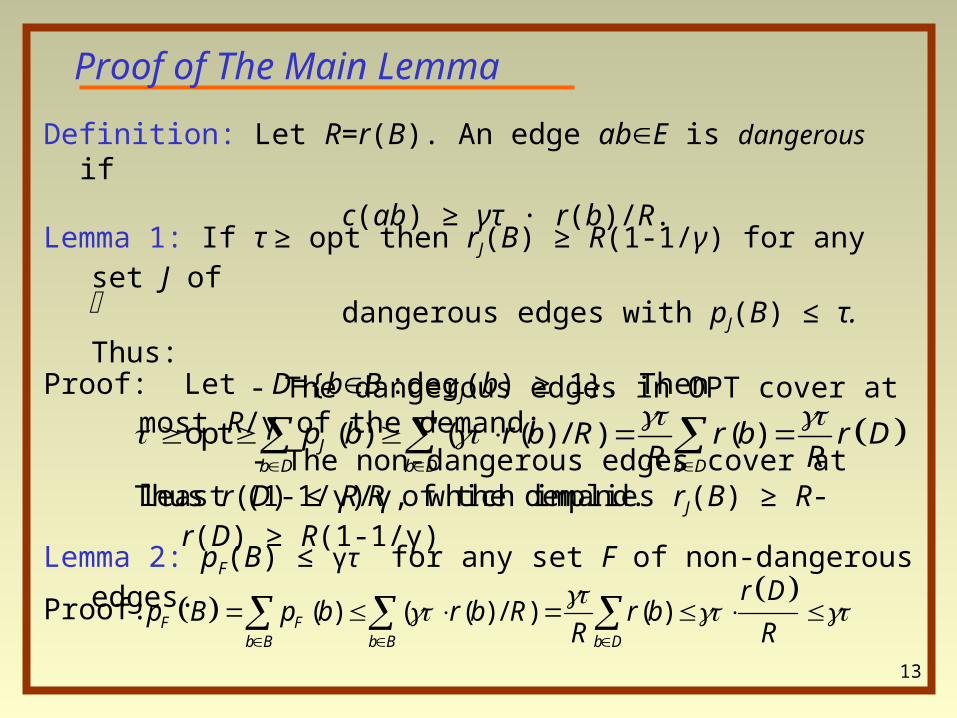
Proof of The Main Lemma
opt ( ) ( ( ) / ) ( )Jb D b D b D
p b r b R r b r DR R
Lemma 1: If τ ≥ opt then rJ(B) ≥ R(1-1/γ) for any set J of dangerous edges with pJ(B) ≤ τ. Thus:
- The dangerous edges in OPT cover at most R/γ of the demand; - The non-dangerous edges cover at least (1-1/γ)R of the demand.
Definition: Let R=r(B). An edge abE is dangerous if
c(ab) ≥ γτ · r(b)/R.
Proof: Let D={bB :degJ(b) ≥ 1}. Then
Lemma 2: pF(B) ≤ γτ for any set F of non-dangerous edges.
( ) ( ( ) / ) ( )F F
b B b B b D
r Dp B p b r b R r b
R R
Proof:
Thus r(D) ≤ R/γ, which implies rJ(B) ≥ R-r(D) ≥ R(1-1/γ)
14
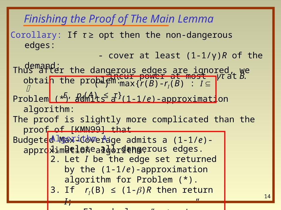
Finishing the Proof of The Main LemmaCorollary: If τ ≥ opt then the non-dangerous edges: - cover at least (1-1/γ)R of the demand; - incur power at most γτ at B.
Thus after the dangerous edges are ignored, we obtain the problem:
Problem (*) admits a (1-1/e)-approximation algorithm:The proof is slightly more complicated than the proof of [KMN99] that Budgeted Max-Coverage admits a (1-1/e)-approximation algorithm.
Algorithm A:1. Delete all dangerous edges.2. Let I be the edge set returned by the (1-1/e)-
approximation algorithm for Problem (*).3. If rI(B) ≤ (1-)R then return I; Else declare “τ ≤ opt”.
(*) max{r(B)-rI(B) : I E, pI(A) ≤ τ}
15
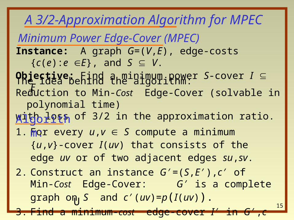
A 3/2-Approximation Algorithm for MPEC
Minimum Power Edge-Cover (MPEC)
The idea behind the algorithm: Reduction to Min-Cost Edge-Cover (solvable in polynomial time) with loss of 3/2 in the approximation ratio.
1. For every u,v S compute a minimum {u,v}-cover I(uv) that consists of the edge uv or of two adjacent edges su,sv.
2. Construct an instance G′=(S,E′),c′ of Min-Cost Edge-Cover: G′ is a complete graph on S and c′(uv)=p(I(uv)).
3. Find a minimum-cost edge-cover I′ in G′,c′.
4. Return I = {I(uv) : uv I′}.
Instance: A graph G=(V,E), edge-costs {c(e):e E}, and S V.Objective: Find a minimum power S-cover I E.
U
Algorithm:
16
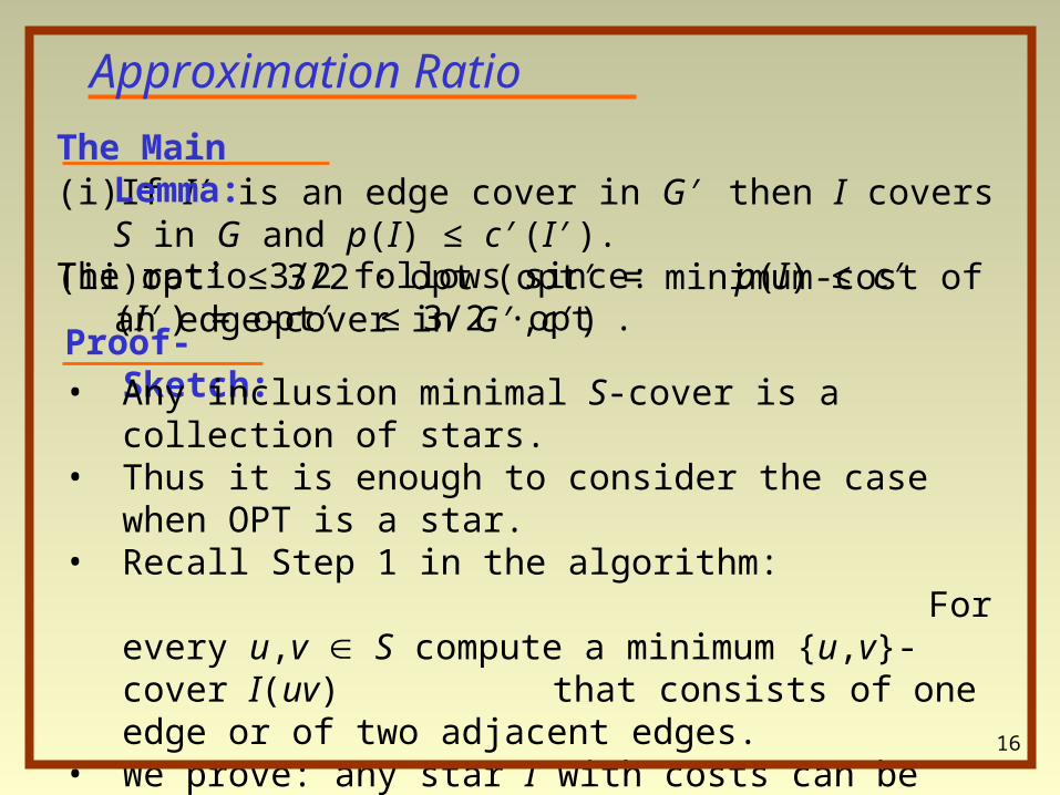
Proof-Sketch: • Any inclusion minimal S-cover is a collection of stars.• Thus it is enough to consider the case when OPT is a star.• Recall Step 1 in the algorithm:
For every u,v S compute a minimum {u,v}-cover I(uv) that consists of one edge or of two adjacent edges.
• We prove: any star I with costs can be decompose into 2-stars and single edges (with at least one edge) so that: The sum of the powers of 2-stars and edges ≤ 3/2·p(I)
(i) If I′ is an edge cover in G′ then I covers S in G and p(I) ≤ c′(I′).
(ii) opt′ ≤ 3/2 · opt (opt′ = minimum-cost of an edge-cover in G′,c′)
The Main Lemma:
Approximation Ratio
The ratio 3/2 follows since: p(I) ≤ c′(I′) = opt′ ≤ 3/2 ·opt .
17
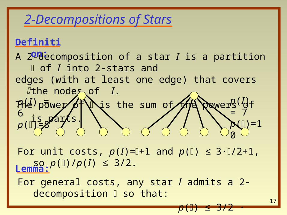
For unit costs, p(I)=+1 and p() ≤ 3·/2+1, so p()/p(I) ≤ 3/2.
2-Decompositions of Stars
A 2-decomposition of a star I is a partition of I into 2-stars and edges (with at least one edge) that covers the nodes of I.
The power of is the sum of the powers of is parts.
Definition:
p(I) = 6p()=8
p(I) = 7p()=10
Lemma:
For general costs, any star I admits a 2-decomposition so that:
p() ≤ 3/2 · p(I)

18
Summary and Open Questions
1. O(log n)-approximation for MPEMC.2. O(log n log n/(n-k))-approximation for MPkCS.3. 3/2-approximation for MPEC.
1. Constant ratio for MPEMC?2. (log n)-hardness for MPEMC?3. Approximation hardness of MPkCS/MCkCS…4. 4/3-approximation for MPEC?
Results:
Open Questions: