The minimum shift design problem

Luca Di Gaspero∗ Johannes Gartner† Guy Kortsarz‡ Nysret Musliu§

Andrea Schaerf¶ Wolfgang Slany‖

Abstract

The min-SHIFT DESIGN problem (MSD) is an important scheduling problem that needs tobe solved in many industrial contexts. The issue is to find a minimum number of shifts andthe number of employees to be assigned to these shifts in order to minimize the deviation fromworkforce requirements.

Our research considers both theoretical and practical aspects of the min-SHIFT DESIGN prob-lem. This problem is closely related to the minimum edge-cost flow problem (MECF ), a networkflow variant that has many applications beyond shift scheduling. We show that MSD reduces to aspecial case of MECF and, exploiting this reduction, we prove a logarithmic hardness of approx-imation lower bound for MSD . On the basis of these results, we propose a hybrid heuristic for theproblem which relies on a greedy heuristic with a min-cost max-flow subroutine based on the net-work flow analogy followed by a local search algorithm that makes use of multiple neighborhoodrelations.

An experimental analysis on structured random instances shows that the hybrid heuristicclearly outperforms our previous commercial implementation and highlights the respective meritsof the composing heuristics for different performance parameters.

Introduction

The typical process of planning and scheduling a workforce in an organization is inherently a multi-phase activity (Tien and Kamiyama, 1982). First, the production or the personnel management have todetermine the temporal staff requirements, i.e., the number of employees needed for each timeslot ofthe planning period. Afterwards, it is possible to proceed to determine the shifts and the total numberof employees needed to cover each shift. The final phase consists in the assignment of the shifts anddays-off to employees.

In the literature, there are mainly two approaches to solve the latter two phases (see Burke et al.,2004). The first approach consists of solving the shift assignment as one single optimization problem(e.g., Glover and McMillan, 1986; Jackson et al., 1997). A second approach, instead, proceeds instages by considering the design of shifts (or staffing) and the assignment as separate problems (Bal-akrishnan and Wong, 1990; Lau, 1996; Musliu et al., 2002). This is computationally easier, althoughthere is no guarantee that the optimal solution to the overall problem can be found.

∗l.digaspero@uniud.it, DIEGM, University of Udine – via delle Scienze 208, I-33100 Udine, Italy†gaertner@ximes.com, Ximes Inc – Schwedenplatz 2/26, A-1010 Wien, Austria‡guyk@camden.rutgers.edu, Computer Science Department, Rutgers University – Camden, NJ 08102, USA§musliu@dbai.tuwien.ac.at, Inst. for Information Systems, Vienna University of Technology, A-1040 Wien,

Austria¶schaerf@uniud.it, DIEGM, University of Udine – via delle Scienze 208, I-33100 Udine, Italy‖wsi@ist.tugraz.at, Inst. for Software Technology, Graz University of Technology – A-8010 Graz, Austria

1

In this work we follow the latter approach and focus on the problem of designing the shifts only.We propose the min-SHIFT DESIGN formulation where the issue is to construct a set of work shiftsto use, their number being minimal (hence the name), and to find the number of workers to assignto each shift in order to meet (or minimize the deviation from) pre-specified staff requirements. Theselection of shifts is subject to constraints on the possible start times and lengths of shifts. Our work ismotivated by practical considerations. It differs in particular from other literature dealing with similarproblems by the explicit constraint of minimizing the number of shifts. The existence of less shiftsleads to schedules that are easier to read, check, manage and administer.

The MSD problem arose in a project at Ximes Inc, a consulting and software development com-pany specializing in shift scheduling. The goal of this project was, among others, to produce a soft-ware end-product called OPA (short for ‘OPerating hours Assistant’). OPA was introduced mid 2001to the market and has since been successfully sold to end-users besides of being heavily used in the dayto day consulting work of Ximes Inc at customer sites (mainly European, but Ximes recently also wona contract with the US ministry of transportation). OPA has been optimized for “presentation”-styleuse where solutions to many variants of problem instances are expected to be more or less immedi-ately available for graphical exploration by the audience. Speed is of crucial importance to allow forimmediate discussion in working groups and refinement of requirements, especially if such a solveris used during a meeting with customers. Without quick answers, understanding of requirementsand consensus building would be much more difficult. OPA and the underlying heuristics have beendescribed in (Gartner et al., 2001; Musliu et al., 2004).

In this work we aim at giving a deeper insight into the problem. We first establish the complexityof the min-SHIFT DESIGN problem by means of a reduction to a network flow problem, namely thecyclic multi-commodity capacitated fixed-charge min-COST max-FLOW problem (Garey and Johnson,1979, Prob. ND32, page 214). As we will show, even a logarithmic approximation of the problem isNP-hard. However, if the issue of minimizing the number of shifts is neglected, the resulting problembecomes solvable in polynomial time.

Based on the above theoretical results, we propose an hybrid solver for the MSD problem, com-posed of two heuristics. The first is a greedy construction heuristic based on the min-COST max-FLOW

analogy. The second is a local search algorithm that makes use of the multi-neighborhood search ap-proach proposed by Di Gaspero and Schaerf (2003a).

We evaluate the performances of the proposed heuristics on different settings and we comparethem and the resulting hybrid solver with OPA. The outcome of the comparison shows that our heuris-tics significantly outperforms the previous approach.

1 Problem statement

The min-SHIFT DESIGN (MSD) consists in the selection of which work shifts to use and how manypeople to assign to each such shift in order to meet pre-specified workforce requirements.

The requirements are given for d planning days D = {1, . . . , d} (the so-called planning horizon),where a planning day can start at a certain time on a regular calendar day and ends 24 hours later,usually on the next calendar day. Each planning day j is split into n equal-size smaller intervalsti = [τi, τi+1), called timeslots, which have the same length h := ‖τi+1 − τi‖ ∈ N expressed inminutes. The time point τ1 on the first planning day represents the start of the planning horizon,whereas time point τn+1 on the last planning day is the end of the planning horizon. In this work wedeal with cyclic schedules, thus τn+1 of the last planning day coincides with τ1 of the first planningday of the next cycle, and the requirements are repeated in each cycle.

2

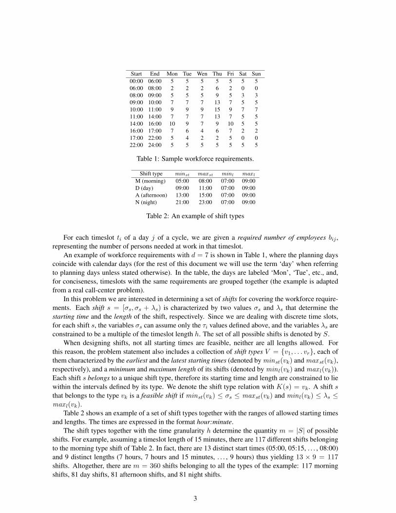
Start End Mon Tue Wen Thu Fri Sat Sun00:00 06:00 5 5 5 5 5 5 506:00 08:00 2 2 2 6 2 0 008:00 09:00 5 5 5 9 5 3 309:00 10:00 7 7 7 13 7 5 510:00 11:00 9 9 9 15 9 7 711:00 14:00 7 7 7 13 7 5 514:00 16:00 10 9 7 9 10 5 516:00 17:00 7 6 4 6 7 2 217:00 22:00 5 4 2 2 5 0 022:00 24:00 5 5 5 5 5 5 5

Table 1: Sample workforce requirements.

Shift type minst max st minl max l

M (morning) 05:00 08:00 07:00 09:00D (day) 09:00 11:00 07:00 09:00A (afternoon) 13:00 15:00 07:00 09:00N (night) 21:00 23:00 07:00 09:00

Table 2: An example of shift types

For each timeslot ti of a day j of a cycle, we are given a required number of employees bij ,representing the number of persons needed at work in that timeslot.

An example of workforce requirements with d = 7 is shown in Table 1, where the planning dayscoincide with calendar days (for the rest of this document we will use the term ‘day’ when referringto planning days unless stated otherwise). In the table, the days are labeled ‘Mon’, ‘Tue’, etc., and,for conciseness, timeslots with the same requirements are grouped together (the example is adaptedfrom a real call-center problem).

In this problem we are interested in determining a set of shifts for covering the workforce require-ments. Each shift s = [σs, σs + λs) is characterized by two values σs and λs that determine thestarting time and the length of the shift, respectively. Since we are dealing with discrete time slots,for each shift s, the variables σs can assume only the τi values defined above, and the variables λs areconstrained to be a multiple of the timeslot length h. The set of all possible shifts is denoted by S.

When designing shifts, not all starting times are feasible, neither are all lengths allowed. Forthis reason, the problem statement also includes a collection of shift types V = {v1, . . . vr}, each ofthem characterized by the earliest and the latest starting times (denoted by minst(vk) and max st(vk),respectively), and a minimum and maximum length of its shifts (denoted by min l(vk) and max l(vk)).Each shift s belongs to a unique shift type, therefore its starting time and length are constrained to liewithin the intervals defined by its type. We denote the shift type relation with K(s) = vk. A shift sthat belongs to the type vk is a feasible shift if minst(vk) ≤ σs ≤ max st(vk) and min l(vk) ≤ λs ≤max l(vk).

Table 2 shows an example of a set of shift types together with the ranges of allowed starting timesand lengths. The times are expressed in the format hour:minute.

The shift types together with the time granularity h determine the quantity m = |S| of possibleshifts. For example, assuming a timeslot length of 15 minutes, there are 117 different shifts belongingto the morning type shift of Table 2. In fact, there are 13 distinct start times (05:00, 05:15, . . . , 08:00)and 9 distinct lengths (7 hours, 7 hours and 15 minutes, . . . , 9 hours) thus yielding 13 × 9 = 117shifts. Altogether, there are m = 360 shifts belonging to all the types of the example: 117 morningshifts, 81 day shifts, 81 afternoon shifts, and 81 night shifts.

3

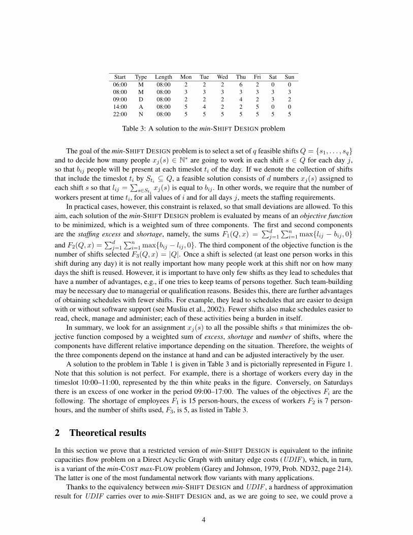
Start Type Length Mon Tue Wed Thu Fri Sat Sun06:00 M 08:00 2 2 2 6 2 0 008:00 M 08:00 3 3 3 3 3 3 309:00 D 08:00 2 2 2 4 2 3 214:00 A 08:00 5 4 2 2 5 0 022:00 N 08:00 5 5 5 5 5 5 5

Table 3: A solution to the min-SHIFT DESIGN problem

The goal of the min-SHIFT DESIGN problem is to select a set of q feasible shifts Q = {s1, . . . , sq}and to decide how many people xj(s) ∈ N∗ are going to work in each shift s ∈ Q for each day j,so that bij people will be present at each timeslot ti of the day. If we denote the collection of shiftsthat include the timeslot ti by Sti ⊆ Q, a feasible solution consists of d numbers xj(s) assigned toeach shift s so that lij =

∑s∈Sti

xj(s) is equal to bij . In other words, we require that the number ofworkers present at time ti, for all values of i and for all days j, meets the staffing requirements.

In practical cases, however, this constraint is relaxed, so that small deviations are allowed. To thisaim, each solution of the min-SHIFT DESIGN problem is evaluated by means of an objective functionto be minimized, which is a weighted sum of three components. The first and second componentsare the staffing excess and shortage, namely, the sums F1(Q, x) =

∑dj=1

∑ni=1 max{lij − bij , 0}

and F2(Q, x) =∑d

j=1

∑ni=1 max{bij − lij , 0}. The third component of the objective function is the

number of shifts selected F3(Q, x) = |Q|. Once a shift is selected (at least one person works in thisshift during any day) it is not really important how many people work at this shift nor on how manydays the shift is reused. However, it is important to have only few shifts as they lead to schedules thathave a number of advantages, e.g., if one tries to keep teams of persons together. Such team-buildingmay be necessary due to managerial or qualification reasons. Besides this, there are further advantagesof obtaining schedules with fewer shifts. For example, they lead to schedules that are easier to designwith or without software support (see Musliu et al., 2002). Fewer shifts also make schedules easier toread, check, manage and administer; each of these activities being a burden in itself.

In summary, we look for an assignment xj(s) to all the possible shifts s that minimizes the ob-jective function composed by a weighted sum of excess, shortage and number of shifts, where thecomponents have different relative importance depending on the situation. Therefore, the weights ofthe three components depend on the instance at hand and can be adjusted interactively by the user.

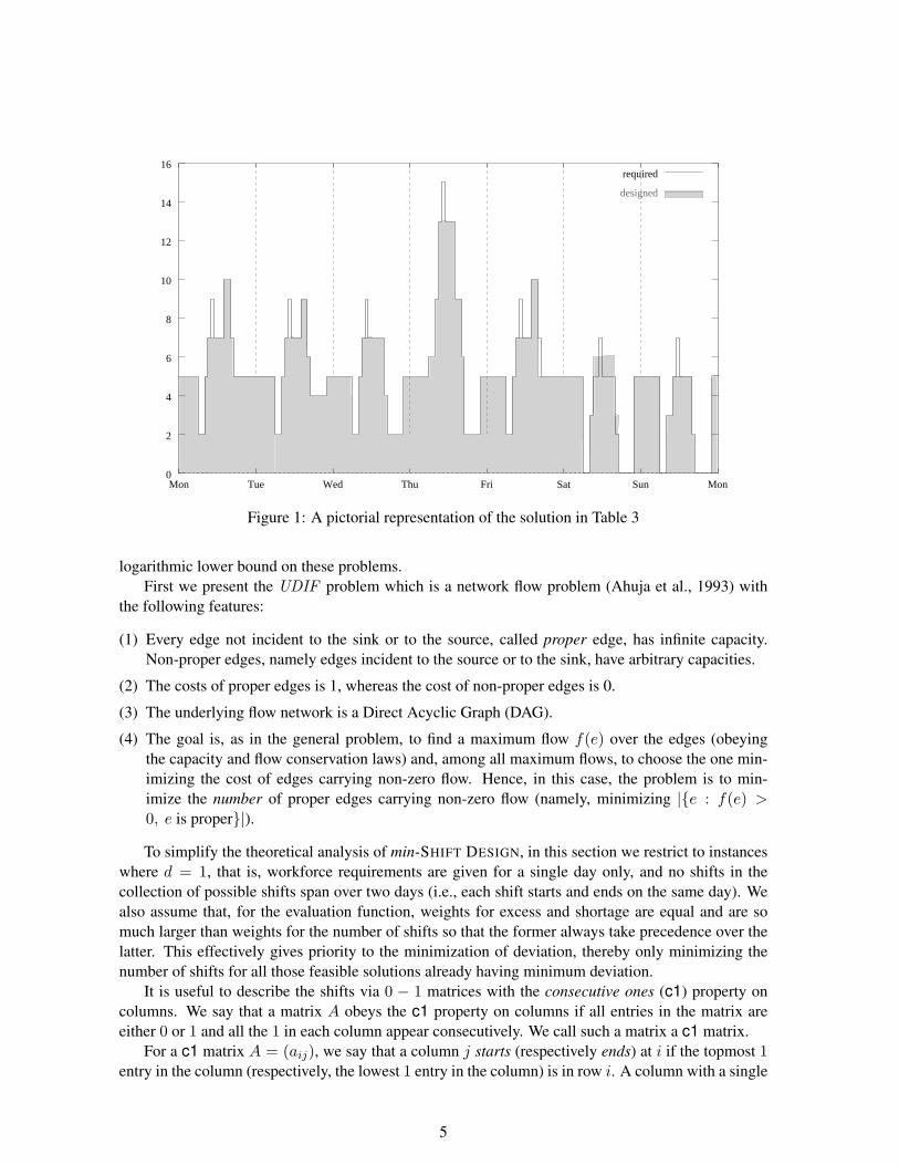
A solution to the problem in Table 1 is given in Table 3 and is pictorially represented in Figure 1.Note that this solution is not perfect. For example, there is a shortage of workers every day in thetimeslot 10:00–11:00, represented by the thin white peaks in the figure. Conversely, on Saturdaysthere is an excess of one worker in the period 09:00–17:00. The values of the objectives Fi are thefollowing. The shortage of employees F1 is 15 person-hours, the excess of workers F2 is 7 person-hours, and the number of shifts used, F3, is 5, as listed in Table 3.

2 Theoretical results

In this section we prove that a restricted version of min-SHIFT DESIGN is equivalent to the infinitecapacities flow problem on a Direct Acyclic Graph with unitary edge costs (UDIF ), which, in turn,is a variant of the min-COST max-FLOW problem (Garey and Johnson, 1979, Prob. ND32, page 214).The latter is one of the most fundamental network flow variants with many applications.

Thanks to the equivalency between min-SHIFT DESIGN and UDIF , a hardness of approximationresult for UDIF carries over to min-SHIFT DESIGN and, as we are going to see, we could prove a

4

0

required

Mon Tue Wed Thu Fri Sat Sun Mon

16

14

12

10

8

6

4

2

designed

Figure 1: A pictorial representation of the solution in Table 3

logarithmic lower bound on these problems.First we present the UDIF problem which is a network flow problem (Ahuja et al., 1993) with

the following features:

(1) Every edge not incident to the sink or to the source, called proper edge, has infinite capacity.Non-proper edges, namely edges incident to the source or to the sink, have arbitrary capacities.

(2) The costs of proper edges is 1, whereas the cost of non-proper edges is 0.

(3) The underlying flow network is a Direct Acyclic Graph (DAG).

(4) The goal is, as in the general problem, to find a maximum flow f(e) over the edges (obeyingthe capacity and flow conservation laws) and, among all maximum flows, to choose the one min-imizing the cost of edges carrying non-zero flow. Hence, in this case, the problem is to min-imize the number of proper edges carrying non-zero flow (namely, minimizing |{e : f(e) >0, e is proper}|).

To simplify the theoretical analysis of min-SHIFT DESIGN, in this section we restrict to instanceswhere d = 1, that is, workforce requirements are given for a single day only, and no shifts in thecollection of possible shifts span over two days (i.e., each shift starts and ends on the same day). Wealso assume that, for the evaluation function, weights for excess and shortage are equal and are somuch larger than weights for the number of shifts so that the former always take precedence over thelatter. This effectively gives priority to the minimization of deviation, thereby only minimizing thenumber of shifts for all those feasible solutions already having minimum deviation.

It is useful to describe the shifts via 0 − 1 matrices with the consecutive ones (c1) property oncolumns. We say that a matrix A obeys the c1 property on columns if all entries in the matrix areeither 0 or 1 and all the 1 in each column appear consecutively. We call such a matrix a c1 matrix.

For a c1 matrix A = (aij), we say that a column j starts (respectively ends) at i if the topmost 1entry in the column (respectively, the lowest 1 entry in the column) is in row i. A column with a single

5

1 entry in the ith place both starts and ends at i. The row in which a column j starts (respectively,ends) is denoted by βj (respectively ηj).

We give a formal description of min-SHIFT DESIGN via c1 matrices as follows. We are given ann×m matrix A in which each column corresponds to a possible shift. Each entry aij in the matrix iseither 1 if i is a valid timeslot for shift s = j or 0 otherwise. Since the set of valid timeslots for a givenshift type (and thus for a given shift belonging to a shift type) is made up of consecutive timeslots, Ais clearly a c1 matrix. Furthermore, we are given a vector b of length n of positive integers; each entrybi corresponds to the workforce requirement for the timeslot i. Within these settings, the min-SHIFT

DESIGN problem can be stated as a system of inequalities: Ax ≥ b with x ∈ Zn, x ≥ 0, where thevectors x correspond to the shift assignments.

The optimization criteria are represented as follows. Let Ai be the ith row in A, and ‖x‖1 denotethe L1 norm of x. We are looking for a vector x ≥ 0 with the following properties:

(1) The vector x minimizes ‖Ax− b‖1 (i.e., the deviation from the staffing requirements).

(2) Among all vectors minimizing ‖Ax − b‖1, x has the minimum number of non-zero entries (cor-responding to the number of selected shifts).

Claim 1 The restricted one-day noncyclic variant of min-SHIFT DESIGN where a zero deviationsolution exists (i.e., d = 1, all shifts start and finish on the same day, and Ax = b admits a solution),is equivalent to the UDIF problem.

The proof below is followed by an explanation of how shortage and excess can be handled bya small linear adaptation of the network flow problem. This effectively allows us to find the min-imum (weighted) deviation from the workforce requirements (without considering minimization ofthe number of shifts) by solving a min-COST max-FLOW (MCMF ) problem, an idea that will bereused in Section 3.1. It is well known that the problem of finding such a maximum flow minimizing∑

e p(e)f(e) is solvable in polynomial time (see, e.g., Papadimitriou and Steiglitz, 1982).

Proof. We are following here a path similar to the one by Hochbaum (2000) in order to get thisequivalence (see also, e.g., Ahuja et al., 1993).

First note that in the special case when Ax = b has a feasible solution, by the definition of MSDthe optimum x∗ satisfies Ax∗ = b.

Let T denote the matrix:

T =

1 −1 0 0 0 00 1 −1 0 0 · · · 00 0 1 −1 0 0

.... . .

...0 0 0 1 −1 00 0 0 · · · 0 1 −10 0 0 0 0 1

The matrix T is a n × n matrix which is regular. In fact, T −1 is the upper diagonal matrix with 1along the diagonal and above, whereas all other elements are equal to 0.

As T is regular, the two sets of feasible vectors for Ax = b and for T Ax = T b are equal. Thematrix F = T A is a matrix with at most two non-zero entries in each column: one being a 1 and theother being a −1. In fact, all columns j in A create a column in F = T A with exactly one −1 entry

6

and exactly one 1 entry except for columns j with 1 in the first row (namely, so that βj = 1). Thesecolumns leave one 1 entry in row ηj , namely, in the row where column j ends. We call these columnsthe special columns.

The matrix F can be interpreted as a flow matrix (see, e.g., Bar-Ilan et al., 2001). We start ourconstruction with a graph consisting of only two vertices s1 and t, representing the source and the sinkof the flow graph. Then we assign a vertex ui to each row i of the matrix and we add an extra vertexu0.

Each column j of the matrix F is represented by an edge ej . Each ej with Fij = 1 and Fkj = −1goes out of uk into ui. Note that the existence of this column in F implies the existence in A of acolumn of ones starting at row k + 1 (and not k) and ending at row j.

For all special columns j ending at ηj , we add an edge from u0 into uηj . In addition, we add anedge of capacity b1 from the source s to u0.

Let b = T b. This vector determines the way all vertices (except u0) are joined to the sink t andsource s. If bi > 0 then there is an edge from ui to t with capacity bi. Otherwise, if bi < 0, there isan edge from s to ui with capacity −bi. Vertices with bi = 0 are not joined to the source or sink. Alledges not incident to the source or sink have infinite capacity.

Note that the addition of the edge from s into u0 with capacity b1 makes the sum of capacities ofedges leaving the source equal to the sum of capacities of edges entering the sink. It is easy to seethat if there exists a saturating flow (namely a flow saturating all the edges entering the sink), then thefeasible vectors for the flow problem are exactly the feasible vectors for Fx = b. Hence, these are thesame vectors feasible for the original set of equations Ax = b.

As we assumed that Ax = b has a solution, there exists a saturating flow, namely, there is asolution saturating all the vertex-sink edges (and, in our case, all the edges leaving the source aresaturated as well). Therefore, the problem is transformed into the following question: Given a networkG constructed as above, find a maximum flow in G and among all maximum flows find the one thatminimizes the number of proper edges carrying non-zero flow.

The resulting flow problem is in fact a UDIF problem. Indeed, the network G is a DAG since alledges go from ui to uj with j > i. In addition, all capacities on edges which are not incident to thesink or source are infinite (see the above construction).

On the other hand, given a UDIF instance with a saturating flow it is possible to find an inversefunction that maps it to an MSD instance. The MSD instance is described as follows.

Assume that the vertices ui are ordered in increasing topological order. Given the DAG G, thecorresponding matrix F is defined by taking the edge-vertices incidence matrix of G. As it turns out,we can find a c1 matrix A so that T A = F . Indeed, for any column j with non-zeros in rows p, q withp < q, necessarily, Fpj = −1 and Fqj = 1 (if there is a column j that does not contain an Fpj = −1,let set p = 0). Hence, add to A the c1 column j′ with βj′ = p + 1 and ηj′ = q.

We note that the restriction of the existence of a flow saturating the flow along edges entering thesink t is not essential. It is easy to guarantee this as follows. Add a new vertex u to the network andan edge (s, u) of capacity

∑(v,t) c(v, t) − f∗ (where f∗ is the maximum flow value). By definition,

the edge (s, u) has cost 0. Add a directed edge from u to every source v. This makes a saturating flowpossible, at the increase of only 1 in the cost.

It follows that in the restricted case when Ax = b has feasible solutions the MSD problem isequivalent to UDIF .

In order to understand how this result can be employed to find solutions to MSD instances where1In this proof and in the following one the symbol s denotes the source of the flow graph instead of a generic shift.

7

no zero deviation solution exists, we need to explain how to find a vector x so that Ax ≥ b and‖Ax− b‖1 is minimum.

When Ax = b does not have a solution, we introduce n dummy variables yi. The ith inequalityis replaced by Aix − yi = bi, that is yi is set to the difference between Aix and bi (and yi ≥ 0). Let−I be the negative identity matrix, namely the matrix with all zeros except−1 in the diagonal entries.Let (A;−I) be the A matrix with −I to its right and let (x; y) be the column of x followed by they variables. The above system of inequalities is represented by (A;−I)(x; y) = b. Multiplying theinequality by T (where T is the matrix defined above) gives (F ;−T )(x; y) = T b = b.

The matrix (F ;−T ) is a flow matrix and its corresponding graph is the graph of F with theaddition of an infinite capacity edge from ui into ui−1 (i = 1, . . . , n). We call these edges the yedges, whereas the edges originally in G are called the x edges. The sum

∑i yi clearly represents the

excess L1 norm ‖Ax− b‖1. Hence, we give a cost C(e) = 1 to each edge corresponding to a yi. Welook for a maximum flow minimizing

∑i C(e)f(e), namely, a min-cost max-flow solution. As we

have assumed (without loss of generality) that all time intervals [ti, ti+1) (i = 1, . . . , n) have equallength, this gives the minimum possible excess. Shortage can be handled in a similar way.

We next show that unless P = NP , there is some constant 0 < c < 1 such that approximatingUDIF within a c lnn−ratio is NP-hard.

Since the case of zero excess MSD is equivalent to UDIF (see Claim 1), similar hardness resultsfollow for this problem as well.

Theorem 2.1 There is a constant c < 1 so that approximating the UDIF problem within c lnn isNP-hard.

Proof. We prove a hardness reduction for UDIF under the assumption P 6= NP using a reductionfrom Set-Cover. We need a somewhat different proof than the one reported in (Krumke et al., 1998)to account for the extra restriction imposed by UDIF . For our purposes it is convenient to formulatethe set cover problem as follows. The set cover instance is an undirected bipartite graph B(U1, U2, A)with edges only crossing between U1 and U2. We may assume that |U1| = |U2| = n. We look for aminimum sized set Q ⊆ U1 so that N(Q) = U2 (namely, every vertex in U2 has a neighbor in Q).If N(Q) = U2 we say that Q covers U2. We may assume that the given instance has a solution. Thefollowing result is proven in (Raz and Safra, 1997).

Theorem 2.2 There is a constant c < 1 so that approximating Set-Cover within c lnn is NP-hard.

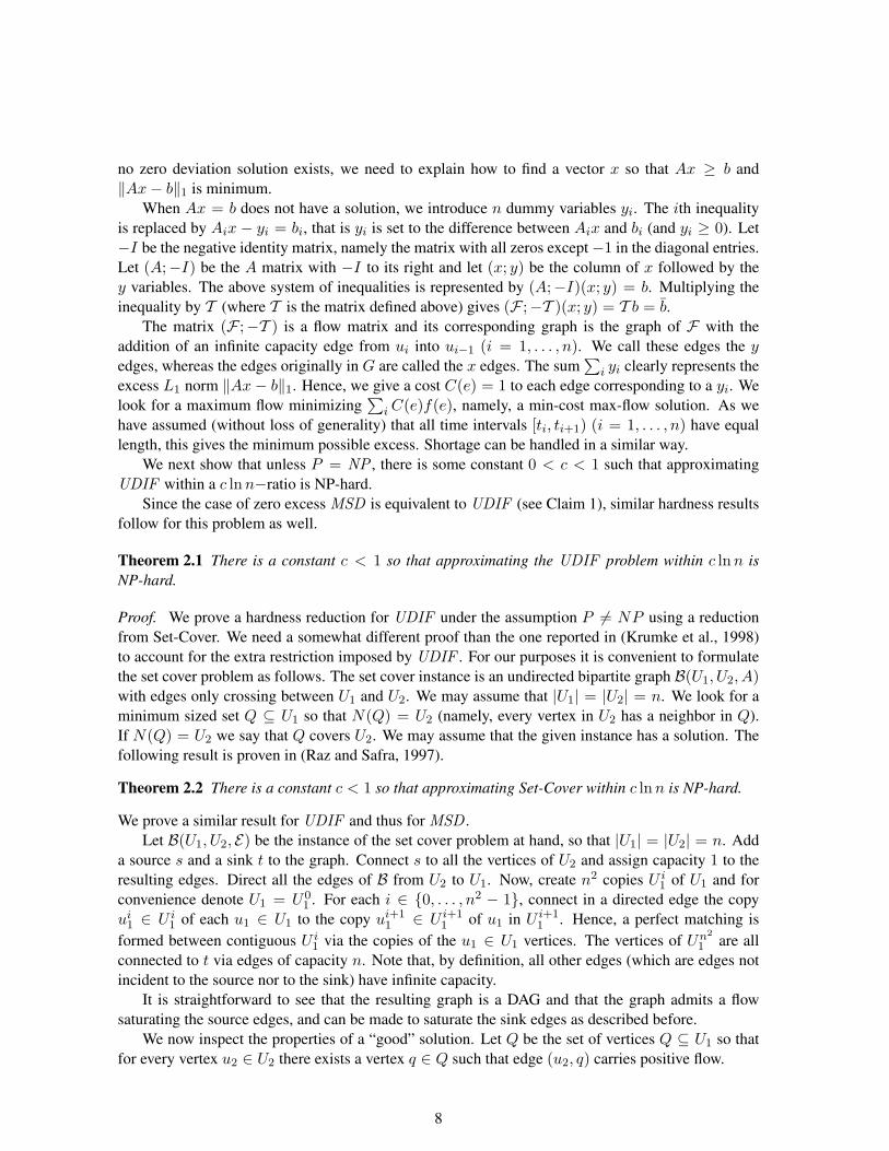
We prove a similar result for UDIF and thus for MSD .Let B(U1, U2, E) be the instance of the set cover problem at hand, so that |U1| = |U2| = n. Add

a source s and a sink t to the graph. Connect s to all the vertices of U2 and assign capacity 1 to theresulting edges. Direct all the edges of B from U2 to U1. Now, create n2 copies U i

1 of U1 and forconvenience denote U1 = U0

1 . For each i ∈ {0, . . . , n2 − 1}, connect in a directed edge the copyui

1 ∈ U i1 of each u1 ∈ U1 to the copy ui+1

1 ∈ U i+11 of u1 in U i+1

1 . Hence, a perfect matching isformed between contiguous U i

1 via the copies of the u1 ∈ U1 vertices. The vertices of Un2

1 are allconnected to t via edges of capacity n. Note that, by definition, all other edges (which are edges notincident to the source nor to the sink) have infinite capacity.

It is straightforward to see that the resulting graph is a DAG and that the graph admits a flowsaturating the source edges, and can be made to saturate the sink edges as described before.

We now inspect the properties of a “good” solution. Let Q be the set of vertices Q ⊆ U1 so thatfor every vertex u2 ∈ U2 there exists a vertex q ∈ Q such that edge (u2, q) carries positive flow.

8

n

U2 U10 U1

n2

Q1Q0 n2Q

s t

1

Figure 2: Schematic illustration of the reduction from the Set-Cover problem to the UDIF problem.

Note that for every u2 ∈ U2 there must be such an edge for otherwise the flow is not optimal.Further note that the flow units entering Q must be carried throughout the copies of Q in all of theU i

1 sets i ≥ 1 using the matching edges as this is the only way to deliver the flow into t. Hence, thenumber of proper edges in the solution is exactly n2 · |Q| + n. The n term comes from the n edgestouching the vertices of u2.

Further, note that Q must be a set cover of U2 in the original graph B. Indeed, every vertex u2

must have a neighbor in Q. Finally, note that it is indeed possible to get a solution with n2 · q∗ + nedges where q∗ is the size of the minimum set cover using an optimum set cover Q∗ as describedabove. Since all the matching edges have infinite capacities, it is possible to deliver to t the n units offlow regardless of how the cover Q is chosen. The following properties end the proof: The numberof vertices in the new graph is O(n3). In addition, the additive term n is negligible for large enoughn in comparison to n2 · |Q| where Q is the chosen set cover. Thus, for large enough n, |Q|n2 ≤c lnn3(|Q∗|n2 +n) would imply that |Q| ≤ 3c lnn(|Q∗|). However, as B was arbitrarely chosen thisstands in contradiction to Theorem 2.2 unless P = NP . Thus the result follows for c < 1/3, and thusalso for c < 1.

3 Practical heuristics

We present a hybrid solver which is divided into two stages, namely a greedy construction for theinitial solution followed by a tabu search procedure (Glover and Laguna, 1997) that iteratively im-proves it, which are described in the following subsections. In our experiments (Sect. 4) we evaluatethe behavior of each stage and of the resulting hybrid algorithm, in order to analyze the sensitivity ofthe tabu search procedure to the starting point used.

3.1 GreedyMCMF

On the basis of the equivalence of the (non-cyclic) min-SHIFT DESIGN problem to UDIF , and therelationship with the min-COST max-FLOW problem, we propose a new greedy heuristic GreedyM-

9

function GreedyMCMF(S,b): MSD Solution

/* 1. Preprocessing step: where to break cyclicity? */

t := FindBestSplitOffTime(S,b); // Search for a split-off on the 1st day of the cycle

/* 2. Greedy part with MCMF subroutine */

f∗ := MCMF(EncodeMSDToFlow(S,b,t)); // Compute best flow so far for MSD instanceσ := ShiftsAndWorkforceIn(f∗); // Shifts are edges with flow 6= 0; workforce is edge flowmin cost := MSD Eval(σ); // Cost of the best MSD solution found so farQ := ShiftsInUseIn(σ); // Shifts in the current solutionT := ∅; // Shifts already triedrepeat

s := UniformlyChooseAShiftFrom(Q \ T ); // Consider a shift s that is used but not tried yetf := MCMF(EncodeMSDToFlow(Q \ {s},b,t)); // Try to solve the problem without shift sσ := ShiftsAndWorkforceIn(f ); // Extract shifts and workforce from flow solutioncurrent cost := MSD Eval(σ); // Compute the cost of the current solutionif current cost < min cost then

min cost := current cost; // Solution with one shift less and lower costf∗ := f ; // Update the best solution found so farQ := ShiftsInUseIn(σ); // Could be less than Q \ {s}

endifT := T ∪ {s}; // Add s to shifts already tried

until Q \ T = ∅; // Cycle until no shift to try is left

/* 3. Postprocessing step to recover cyclicity, perform a local search with the ExchangeStaff move */

σ := SteepestDescent(ShiftsAndWorkforceIn(f∗), ExchangeStaff);return σ;

Figure 3: The Greedy min-COST max-FLOW (MCMF ) subroutine computes a solution for the min-SHIFT DESIGN (MSD) problem

CMF() that uses a polynomial min-COST max-FLOW subroutine (MCMF()). The pseudocode of thealgorithm is reported in Figure 3. The algorithm is based on the observation that the min-COST max-FLOW subroutine can easily compute the optimal staffing with minimum (weighted) deviation whenslack edges (the y edges of Section 2) have associated costs corresponding, respectively, to the weightsof shortage and excess. Note that, however, the algorithm is not able to simultaneously minimize thenumber of shifts that are used.

Since the MCMF() subroutine cannot consider cyclicity, we must first perform a preprocessingstep that determines a good split-off time at which the cycle of d days should be broken. This is doneheuristically by calling MCMF() with different starting times chosen between 5:00 and 8:00 on thefirst day of the cycle (in practice, we can observe that there is almost always a complete exchangeof workforce between 5:00 and 8:00 on Monday mornings). All possibilities in this interval are triedwhile eliminating all shifts that span the chosen starting point when translating from min-SHIFT DE-SIGN to the network flow instances. The number of possibilities depends on the length of the timeslotsof the instance (i.e., the time granularity). The starting point with the smallest cost as determined byMCMF() is used as the split-off time for the rest of the calls to MCMF() in GreedyMCMF. Thismethod has been shown to provide adequate results in practice.

In the main loop, the greedy heuristic then removes all shifts that did not contribute to the min-SHIFT DESIGN instance corresponding to the current flow computed with MCMF(). It randomlychooses one shift (without repetitions) and tests whether removal of this shift still allows the MCMF()

10

to find a solution with the same deviation. If this is the case, that shift is removed and not consideredanymore, otherwise it is left in the set of shifts used to build the network flow instances, but it will notbe considered for removal again.

Finally, when no shifts can be removed anymore without increasing the deviation, a final postpro-cessing step is made to restore cyclicity. It consists of a simple repair step performed by a fast steepestdescent runner that uses the ExchangeStaff neighborhood relation (see below). The runner selects ateach iteration the best neighbor, with a random tie-break in case of same cost. It stops as soon as itreaches a local minimum, i.e., when it does not find any improving move.

As our MCMF() subroutine, we use CS2 version 3.9 ( c© 1995 – 2001 IG Systems, Inc., http://www.avglab.com/andrew/soft.html), an efficient implementation of a scaling push-relabelalgorithm (Goldberg, 1997), slightly edited to be callable as a library.

3.2 Local search heuristic solver

The second stage of the proposed heuristic is based on the local search paradigm (Aarts and Lenstra,1997; Hoos and Stutzle, 2005) and relies on multiple neighborhood relations. In order to describe it,we first define the search space, then describe the set of neighborhood relations for the exploration ofthis search space, followed by the search strategies we employ.

3.2.1 Search space and initial solution

We consider as a state for min-SHIFT DESIGN a pair (Q,X) made up of a set of shifts Q = {s1, s2, . . .}and their staff assignment X = {x1, x2, . . .}. The shifts of a state are split into two categories:

• Active shifts: at least one employee is assigned to a shift of this type on at least one day.

• Inactive shifts: no employees are assigned to a shift of this type on any day. These shifts do notcontribute to the solution and to the objective function. Their role is explained later.

More formally, we say that a shift si ∈ Q is active (resp. inactive) if and only if∑d

j=1 xj(si) 6= 0(= 0).

For the purpose of analyzing the behavior of the local search heuristic alone, we provide also amean to generate a random initial solution for the local search algorithm. That is, we create a fixednumber of random distinct active and inactive shifts for each shift type. Afterwards, for the activeshifts, we assign a random number of employees for each day. The parameters needed to build asolution are the number of active and inactive shifts for each shift type and the range of the number ofemployees per day to be assigned to each random active shift.

For example, in the experimental session described in Section 4, we build a solution with fouractive and two inactive shifts per type, with one to three employees per day assigned to each activeshift. If the possible shifts for a given shift type are less than six, we reduce the generated shiftsaccordingly, giving precedence to the inactive ones.

3.2.2 Neighborhood exploration

Local search methods rely on the definition of neighborhood relation, which is the core feature for theexploration of the search space. The neighborhood of a solution Q is the set of solutions which areobtained applying a set of local perturbations, called moves, on Q.

11

In this work we consider three different neighborhood relations that are combined in the spirit ofthe multi-neighborhood search (Di Gaspero and Schaerf, 2003a). The way these relations are em-ployed during the search is thoroughly explained in Section 3.2.3. In the following, we formallydescribe each neighborhood relation by means of the attributes needed to identify a move, the pre-conditions for its applicability, the effects of the move and, where necessary, some rules for handlingspecial cases.

Given a state (Q,X) of the search space the types of moves considered in this work are thefollowing:

ChangeStaff (CS): The staff of a shift is increased or decreased by one employee

Attributes: 〈si, j, a〉, where si ∈ Q is a shift, j ∈ {1, . . . , d} is a day, a ∈ {↑, ↓}.Preconditions: wj(si) > 0 if and only if a =↓.Effects: if a =↑ then w′

j(si) := wj(si) + 1, else w′j(si) := wj(si)− 1

Special cases: if si is an inactive shift (and a =↑, by precondition), then si becomes active anda new randomly created inactive shift of type K(si) is inserted (distinct from the othershifts).

ExchangeStaff (ES): One employee in a given day is moved from one shift to another one of thesame type.

Attributes: 〈si1 , si2 , j〉, where si1 , si2 ∈ Q, and j ∈ {1, . . . , d}.Preconditions: wj(si1) > 0, K(si1) = K(si2).

Effects: w′j(si1) := wj(si1)− 1 and w′

j(si2) := wj(si2) + 1.

Special cases: If si2 is an inactive shift, si2 becomes active and a new random distinct inactiveshift of type K(si1) is inserted (if such a distinct shift exists). If the move makes si1

inactive then, in the new state, the shift si1 is removed from the set Q.

ResizeShift (RS): The length of the shift is increased or decreased by 1 time-slot, either on theleft-hand side or on the right-hand side.

Attributes: 〈si, l, p〉, where si = [σi, σi + λi) ∈ Q, l ∈ {↑, ↓}, and p ∈ {←,→}.Effects: We denote with δ the size modification to be applied to the shift si, that is δ = +1

when the shift is enlarged by one timeslot and δ = −1 when the shift is shrunk.If p =← the action identified by l is performed on the left-hand side of si, that is σ′

i :=σi + δh and λi does not change. Conversely, if p =→ the move takes place to the right-hand side, therefore σi remains unchanged and λ′i := λi + δh.

Preconditions: For this kind of move we require that the shift s′i, obtained from si by theapplication of the move must be feasible with respect to the shift type K(si).

In a previous work of some of us (Musliu et al., 2004), we define many neighborhood relationsfor this problem including CS, ES, and a variant of RS. In this paper, instead, we restrict ourselvesto the above three relations for the following two reasons.

CS and RS represent the most atomic changes, so that all other move types can be built as chainsof moves of these types. For example an ES move can be obtained by a pair of CS moves thatdecreases one employee from a shift and assigns him/her in the same day to the other shift.

12

Even though ES is not a basic move type, it turned out to be very effective for the search. Infact, the move that passes one employee from a shift to another one makes a very small change tothe current state, which represents a fine grain adjustments that could not be found by the other movetypes.

Inactive shifts are conceived to provide a single uniform way to move staff between shifts and tonew shifts. This approach limits the insertion of employees in new shifts only to the current inactiveones, rather than considering all possible shifts belonging to the shift types (which are many more).Obviously, we could also insert as many inactive shifts as compatible with the shift type, thus allowingto insert any possible shift. Preliminary experimental results, though, show that there is a trade-offbetween computational cost and search quality, which seems to have its best trade-off in having 2inactive shifts per type.

3.2.3 Search strategies

In a preliminary test phase, we experimented CS, ES, and RS neighborhoods driven by three differentmeta-heuristics, namely randomized hill climbing, tabu search and simulated annealing. The one thatgave best results is tabu search, and in this work we report only the results with tabu search.

A full description of tabu search is out of the scope of this paper and we refer to (Glover andLaguna, 1997) for a general introduction. We later in this section describe its specialization to ourproblem.

Differently from Musliu et al. (2004), that use tabu search as well, we employ the three neighbor-hood relations selectively in various phases of the search, rather than exploring the overall neighbor-hood at each iteration.

Our strategy is to combine the neighborhood relations CS, ES, and RS, according to the followingscheme made of compositions and interleaving. That is, our algorithm interleaves three different tabusearch runners using the following neighborhoods:

• the ES alone

• the RS alone

• the set-union of the two neighborhoods CS and RS

The runners are invoked sequentially and each one starts from the best state obtained from theprevious one. The overall process stops when a full round of all of them does not find any improve-ment. Each single runner stops when it does not improve the current best solution for a given numberof iterations (called idle iterations).

The reason for using limited neighborhood relations is not to improve the computational effi-ciency, which could be obtained in other ways, for example by a clever ordering of promising moves.The main reason, instead, is the introduction of a certain degree of diversification in the search. Infact, certain move types would be selected very rarely in a full-neighborhood exploration strategy,even though they could help to escape from local minima. For example, a runner that uses all threeneighborhood relations together would almost never perform a CS move that worsens the objectivefunction, simply because it can always find an ES move that worsen it by a smaller amount. On theother hand, the neglected CS move could lead to a more promising region of the search space. Thisintuition is supported by the experimental analysis that shows that our results are much better thanthose in (Musliu et al., 2004).

13

Parameter TS(ES) TS(RS) TS(CS∪RS)Tabu range 10-20 5-10 20-40 (CS)

5-10 (RS)Idle iterations 300 300 2000

Table 4: Tabu search parameter settings

This composite solver is further improved by performing a few changes on the final state of eachrunner, before handing it over as the initial state of the following runner. In details, we make thefollowing two adjustments:

• Identical shifts are merged into one. When the procedure applies RS moves, it is possible thattwo shifts become identical. This situation is not detected at each move, because it is a costlyoperation, and is therefore left to this inter-runner step.

• Inactive shifts are recreated. That is, the current inactive shifts are deleted, and new distinctones are created at random in the same quantity. This step, again, is meant to improve thediversification of the search algorithm.

Concerning the prohibition mechanism of tabu search, for all three runners, the size of the tabulist is kept dynamic by assigning to each move a number of tabu iterations randomly selected within agiven range. The ranges vary for the three runners, and they were selected experimentally. The rangesare roughly suggested by the cardinality of the different neighborhoods, in the sense that a largerneighborhood deserves a longer tabu tenure. According to the standard aspiration criterion defined in(Glover and Laguna, 1997), the tabu status of a move is dropped if it leads to a state better than thecurrent best.

As already mentioned, each runner stops when it has performed a fixed number of iterationswithout any improvement.

Tabu lengths and idle iterations are selected once for all, and the same values were used for allthe instances. The selection turned out to be robust enough for all tested instances. The selectedparameter values are reported in Table 4.

4 Experimental results

In this section, we describe the results obtained by our solvers on a set of benchmark instances. First,we introduce the instances used in this experimental analysis, then we illustrate the performanceparameters that we want to highlight and we present the outcomes of the experiments. We concludethe section with an analysis that aims at classifying the instances in terms of their computationalhardness.

4.1 Description of the instances

The benchmark consists of three different sets, each containing thirty randomly generated instances.Instances were generated in a structured way so as to ensure that they look as similar as possible toreal instances, while allowing for the construction of arbitrarily difficult cases.

Set 1 contains the 30 instances that were described and investigated in (Musliu et al., 2004).They vary in their complexity and we mainly include them to be able to compare the new heuristicswith the results reported in (Musliu et al., 2004) for the OPA implementation. These instances were

14

basically generated by first constructing a feasible solution, called the seed solution, and then takingthe resulting staffing numbers as workforce requirements. This implies that a solution with zerodeviation from workforce requirements is known in advance. In a few cases, our heuristics could findbetter solutions for some instances, so the seed solution may be non-optimal. In the following werefer to the best solutions we could come up with for these instances, either the seed solution or theimproved one, as ‘best known’ solutions.

Set 2 contains instances similar to Set 1, but here the best known solutions of instances 1 to 10were constructed to feature 12 shifts, those of instances 11 to 20 to feature 16 shifts, and those ofinstances 21 to 30 to feature 20 shifts. This allows us to study the relation between the number ofshifts in the best known solutions and the running times of the heuristics.

While knowing these best known solutions eases the evaluation of the proposed heuristics, italso might form a biased preselection toward instances where zero deviation solutions exist for sure,thereby letting all or some of the heuristics behave in ways that are unusual for instances for whichno such solution can be constructed. The Set 3 is therefore composed of instances where presumablysolutions without deviations do not exist. Instances of Set 3 were constructed with the same randominstance generator as the two previous sets but allowing the constructed solutions to contain invalidshifts that deviate from normal starting times and lengths by up to 4 timeslots. The number of shiftsis similar to those in Set 2, i.e., instances 1 to 10 feature 12 shifts (invalid and valid ones) etc. Thisconstruction ensures that it is unlikely that zero deviation solutions exist for these instances. It mightalso be of interest to see whether a significant difference in performance for some of the heuristicscan be recognized compared to Set 2, which would provide evidence that the way Sets 1 and 2 wereconstructed constituted a bias for the heuristics.

All sets of instances are available in self-describing text files from http://www.dbai.tuwien.

ac.at/proj/Rota/benchmarks.html. A detailed description of the random instance generatorused to construct them can be found in (Musliu et al., 2004).

4.2 Experimental setting

In this work we make two types of experiments, aiming at evaluating two different performance pa-rameters:

1. median time necessary to reach the best known solution,

2. average objective value obtained within a time bound.

The latter parameter consists of the weighted sum of the three components F1 (excess), F2 (short-age) and F3 (number of shifts) (see Section 1). The components F1 and F2 are measured in number ofworkers in excess/shortage per minute, whereas the component F3 is multiplied by 60 minutes. Thisway, the penalty of each shift is the same as one worker in excess/shortage for a whole hour.

Our experiments have been run on different machines. The local search solvers are implemented inC++ using the EASYLOCAL++ framework (Di Gaspero and Schaerf, 2003b) and they were compiledusing the GNU g++ compiler version 3.2.2 on a 1.5 GHz AMD Athlon PC running Linux kernel2.4.21. The greedy min-COST max-FLOW algorithm, instead, was coded in MS Visual Basic and runson a MS Windows NT 4.0 computer.

The running times have been normalized according to the DIMACS netflow benchmark2 to thetimes of the Linux PC (calibration timings on that machine for above benchmark: t1.wm:user

2ftp://dimacs.rutgers.edu/pub/netflow/benchmarks/c/

15

0.030 sec t2.wm:user 0.360 sec). Because of the normalization the reported running timesshould be taken as indicatory only.

Our experiments deal with the following three heuristic solvers:

LS The local search procedure repeated several times starting from different (random) initial solu-tions. The procedure is stopped when the time granted is elapsed or the best solution is reached.

GrMCMF GreedyMCMF() is called repeatedly until the stopping criterion is reached. Since theselection of the next shift to be removed in the main loop of GreedyMCMF() is done randomly,we call the basic heuristic repeatedly and use bootstrapping as described in (Johnson, 2002) tocompute expected values for the computational results (counting the preprocessing step onlyonce for each instance since it computes the same split-off time for all runs).

GrMCFC+LS The two solvers are combined using the solutions delivered by GrMCMF as initialstates for LS trials. In order to maintain diversification, we exploit the non-determinism ofGrMCMF to generate many different solutions. The initial state of each trial of LS is randomlyselected among those states.

4.3 Computational results

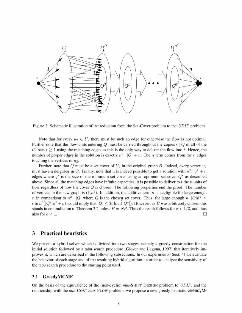
The first experiment evaluates the running times needed to reach the best known solution. We ran thesolvers on data Set 1 for 10 trials until they could reach the best known solution, and we recorded therunning times for each trial.

Table 5 shows the average times and their standard deviations (in parentheses) expressed in sec-onds, needed by our solvers to reach the best known solution. The first two columns show the instancenumber and the best known cost for that instance. The third column reports the cost of the best solu-tion found by OPA (Musliu et al., 2004). Bold numbers in the second column indicate that the bestknown solution for this instance was not found by OPA. Dash symbols denote that the best knownsolution could not be found in any of the 10 trials for those instances.

First, note that all three solvers in general produce better results than the commercial tool. In fact,LS always finds the best solution, GrMCMF in 20 cases and GrMCMF+LS in 29 cases out of 30instances. OPA, instead, could find the best solution only for 17 instances. However, looking at thetime performance on the whole set of instances, it is clear that LS is roughly 30 times slower thanGrMCMF and 1.5 times slower than the hybrid heuristic. GrMCMF+LS is significantly outperformedby LS only for some few instances for which GrMCMF could not find the best known solution, thusbiasing the local search part of the heuristic away from search space near the best known solution.

As a general remark, the LS algorithm proceeds by relatively sudden improvements, especially inthe early phases of the search, while the behavior of the GrMCMF+LS is much smoother (we omitgraphs showing this for brevity).

Starting local search from the solution provided by GrMCMF has also an additional benefit interms of the increase of robustness, roughly measured by the standard deviations of the running times.In fact, for this set of instances, while the standard deviation for LS is about 50% of the averagerunning time, this value decreases to 35% for GrMCMF+LS. The behavior of the GrMCMF solveris similar to the one of the hybrid heuristic and the standard deviation is about 35% of the averagerunning time.

16

OPAInstance BestMusliu et al. (2004)

GrMCMF LS GrMCMF+LS

1 480 480 0.07 (0.00) 5.87 (4.93) 1.06 (0.03)2 300 390 — (—) 16.41 (9.03) 40.22 (27.93)3 600 600 0.11 (0.01) 8.96 (5.44) 1.64 (0.05)4 450 1,170 — (—) 305.37 (397.71) 108.29 (75.32)5 480 480 0.20 (0.16) 5.03 (2.44) 1.75 (1.43)6 420 420 0.06 (0.01) 2.62 (0.99) 0.62 (0.02)7 270 570 1.13 (1.10) 10.25 (5.77) 6.95 (2.88)8 150 180 — (—) 18.98 (15.70) 10.64 (0.56)9 150 225 3.53 (2.63) 11.85 (2.28) 8.85 (1.56)

10 330 450 — (—) 66.05 (41.27) 84.11 (99.85)11 30 30 0.21 (0.00) 1.79 (0.37) 0.85 (0.02)12 90 90 0.25 (0.00) 6.10 (1.50) 3.84 (0.10)13 105 105 0.35 (0.13) 7.20 (2.30) 3.82 (0.09)14 195 390 — (—) 561.99 (404.33) 60.97 (51.08)15 180 180 0.04 (0.00) 0.89 (0.11) 0.40 (0.01)16 225 375 — (—) 198.50 (117.84) 151.78 (125.88)17 540 1,110 — (—) 380.72 (467.64) 288.42 (27.58)18 720 720 1.71 (1.30) 7.72 (2.89) 7.32 (3.79)19 180 195 — (—) 38.33 (20.72) 31.12 (17.99)20 540 540 0.11 (0.01) 15.24 (6.18) 1.69 (0.07)21 120 120 0.28 (0.00) 6.19 (1.32) 2.18 (0.11)22 75 75 0.65 (0.45) 3.67 (0.80) 3.80 (0.86)23 150 540 6.19 (2.91) 19.16 (10.92) 22.15 (15.34)24 480 480 0.11 (0.04) 2.85 (0.38) 1.44 (0.72)25 480 690 — (—) 503.40 (136.17) — (—)26 600 600 1.50 (1.14) 9.59 (6.80) 9.20 (6.20)27 480 480 0.07 (0.00) 4.02 (0.71) 2.34 (0.06)28 270 270 2.24 (0.94) 9.25 (7.67) 3.81 (0.62)29 360 390 — (—) 20.59 (17.20) 10.00 (4.92)30 75 75 0.26 (0.00) 2.78 (0.30) 1.95 (0.01)

Table 5: Times to reach the best known solution for Set 1. Data are averages and standard deviations(in parentheses) for 10 trials.

4.4 Time-limited experiments

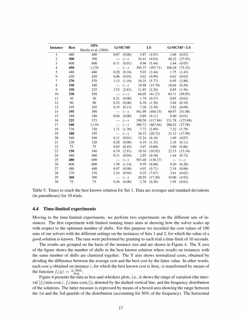
Moving to the time-limited experiments, we perform two experiments on the different sets of in-stances. The first experiment with limited running times aims at showing how the solver scales upwith respect to the optimum number of shifts. For this purpose we recorded the cost values of 100runs of our solvers with the different settings on the instances of Sets 1 and 2, for which the value of agood solution is known. The runs were performed by granting to each trial a time-limit of 10 seconds.

The results are grouped on the basis of the instance size and are shown in Figure 4. The X axisof the figure shows the number of shifts in the best known solution where results on instances withthe same number of shifts are clustered together. The Y axis shows normalized costs, obtained bydividing the difference between the average cost and the best cost by the latter value. In other words,each cost y obtained on instance i, for which the best known cost is besti, is transformed by means ofthe function fi(y) := y−besti

besti.

Figure 4 presents the data as box-and-whiskers plots, i.e., it shows the range of variation (the inter-val [fi(min-costi), fi(max-costi)]), denoted by the dashed vertical line, and the frequency distributionof the solutions. The latter measure is expressed by means of a boxed area showing the range betweenthe 1st and the 3rd quartile of the distribution (accounting for 50% of the frequency). The horizontal

17

GrMCMF+LS

00.

020.

040.

060.

080.

10.

120.

14

8 10 12 14 16 18 20

GreedyMCMFLS

Figure 4: Aggregated normalized costs for 10s time-limit on data Sets 1 and 2.

line within the box denotes the median of the distribution and the notches around the median indicatethe range for which the difference of medians is significant at a probability level of p < 0.05.

The figure shows that, for short runs, the hybrid solver is superior to GrMCMF and LS alone,both in terms of solution quality and robustness: the ranges of variation are shorter and the frequencyboxes are tinier.

Looking at these results from another point of view, it is worth noting that GrMCMF+LS is able tofind more low-cost (and even min-cost) solutions that are significantly better than those found by LSand GrMCMF. Furthermore, it is apparent that the hybrid heuristic scales better than its components,since the deterioration in the solution quality with respect to the number of shifts grows very slowlyand always remains under an acceptable level (7% on the worst case, and about 2% for 75% of theruns).

The second time-limited experiment aims at investigating the behavior of the solver when providedwith a very short running time on ‘unknown’ instances (we use here the term unknown by contrastwith the sets of instances constructed around the seed solution). We performed this experiment on theSet 3 and recorded the cost values found by our solver over 100 trials. Each trial was granted 1 secondof running time, in order to simulate a practical situation in which the user needs a fast feedback fromthe solver. As already mentioned in the introduction, for this problem, speed is extremely important,to allow for real-time refinement of requirements during a meeting with customers.

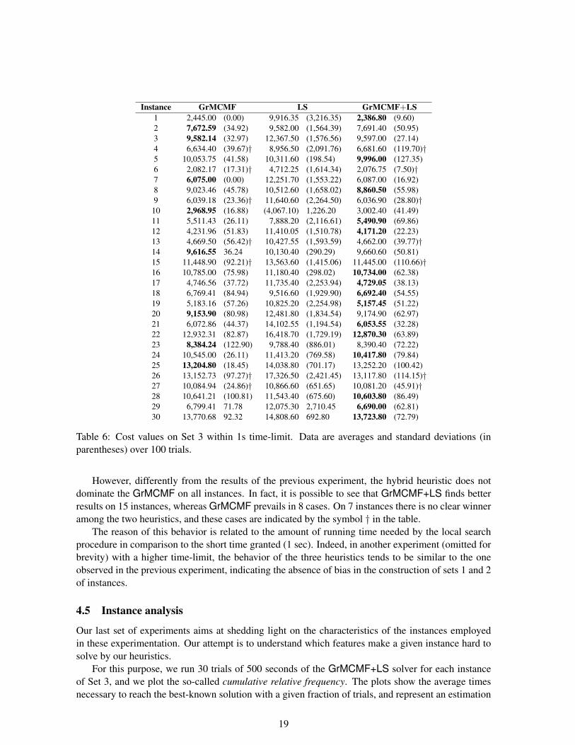
In Table 6 we report the average and the standard deviation (in parentheses) of the cost valuesfound by each heuristic. The best algorithm on each instance is highlighted in boldface. The symbol †denotes the cases for which the difference between the distribution of solutions was not statisticallysignificant (Mann-Whitney test with p < 0.01) and therefore there was no “clear winner”.

In this case the hybrid heuristic performs better than LS on all instances, and it shows a betterbehavior in terms of algorithm robustness (in fact, the standard deviation of GrMCMF+LS is usuallymore than an order of magnitude smaller than the one of LS). Moreover, even the GrMCMF achievesbetter results than the LS heuristic, due to the running time performance of the local search procedure.

18

Instance GrMCMF LS GrMCMF+LS1 2,445.00 (0.00) 9,916.35 (3,216.35) 2,386.80 (9.60)2 7,672.59 (34.92) 9,582.00 (1,564.39) 7,691.40 (50.95)3 9,582.14 (32.97) 12,367.50 (1,576.56) 9,597.00 (27.14)4 6,634.40 (39.67)† 8,956.50 (2,091.76) 6,681.60 (119.70)†5 10,053.75 (41.58) 10,311.60 (198.54) 9,996.00 (127.35)6 2,082.17 (17.31)† 4,712.25 (1,614.34) 2,076.75 (7.50)†7 6,075.00 (0.00) 12,251.70 (1,553.22) 6,087.00 (16.92)8 9,023.46 (45.78) 10,512.60 (1,658.02) 8,860.50 (55.98)9 6,039.18 (23.36)† 11,640.60 (2,264.50) 6,036.90 (28.80)†

10 2,968.95 (16.88) (4,067.10) 1,226.20 3,002.40 (41.49)11 5,511.43 (26.11) 7,888.20 (2,116.61) 5,490.90 (69.86)12 4,231.96 (51.83) 11,410.05 (1,510.78) 4,171.20 (22.23)13 4,669.50 (56.42)† 10,427.55 (1,593.59) 4,662.00 (39.77)†14 9,616.55 36.24 10,130.40 (290.29) 9,660.60 (50.81)15 11,448.90 (92.21)† 13,563.60 (1,415.06) 11,445.00 (110.66)†16 10,785.00 (75.98) 11,180.40 (298.02) 10,734.00 (62.38)17 4,746.56 (37.72) 11,735.40 (2,253.94) 4,729.05 (38.13)18 6,769.41 (84.94) 9,516.60 (1,929.90) 6,692.40 (54.55)19 5,183.16 (57.26) 10,825.20 (2,254.98) 5,157.45 (51.22)20 9,153.90 (80.98) 12,481.80 (1,834.54) 9,174.90 (62.97)21 6,072.86 (44.37) 14,102.55 (1,194.54) 6,053.55 (32.28)22 12,932.31 (82.87) 16,418.70 (1,729.19) 12,870.30 (63.89)23 8,384.24 (122.90) 9,788.40 (886.01) 8,390.40 (72.22)24 10,545.00 (26.11) 11,413.20 (769.58) 10,417.80 (79.84)25 13,204.80 (18.45) 14,038.80 (701.17) 13,252.20 (100.42)26 13,152.73 (97.27)† 17,326.50 (2,421.45) 13,117.80 (114.15)†27 10,084.94 (24.86)† 10,866.60 (651.65) 10,081.20 (45.91)†28 10,641.21 (100.81) 11,543.40 (675.60) 10,603.80 (86.49)29 6,799.41 71.78 12,075.30 2,710.45 6,690.00 (62.81)30 13,770.68 92.32 14,808.60 692.80 13,723.80 (72.79)

Table 6: Cost values on Set 3 within 1s time-limit. Data are averages and standard deviations (inparentheses) over 100 trials.

However, differently from the results of the previous experiment, the hybrid heuristic does notdominate the GrMCMF on all instances. In fact, it is possible to see that GrMCMF+LS finds betterresults on 15 instances, whereas GrMCMF prevails in 8 cases. On 7 instances there is no clear winneramong the two heuristics, and these cases are indicated by the symbol † in the table.

The reason of this behavior is related to the amount of running time needed by the local searchprocedure in comparison to the short time granted (1 sec). Indeed, in another experiment (omitted forbrevity) with a higher time-limit, the behavior of the three heuristics tends to be similar to the oneobserved in the previous experiment, indicating the absence of bias in the construction of sets 1 and 2of instances.

4.5 Instance analysis

Our last set of experiments aims at shedding light on the characteristics of the instances employedin these experimentation. Our attempt is to understand which features make a given instance hard tosolve by our heuristics.

For this purpose, we run 30 trials of 500 seconds of the GrMCMF+LS solver for each instanceof Set 3, and we plot the so-called cumulative relative frequency. The plots show the average timesnecessary to reach the best-known solution with a given fraction of trials, and represent an estimation

19

0 10 20 30 40 50 60

0.0

0.2

0.4

0.6

0.8

1.0

Instance 16

Time

Cum

ulat

ive

frequ

ency

(a) Easy instance

0 100 200 300 400 500

0.0

0.2

0.4

0.6

0.8

1.0

Instance 02

Time

Cum

ulat

ive

freq

uenc

y

(b) Hard instance

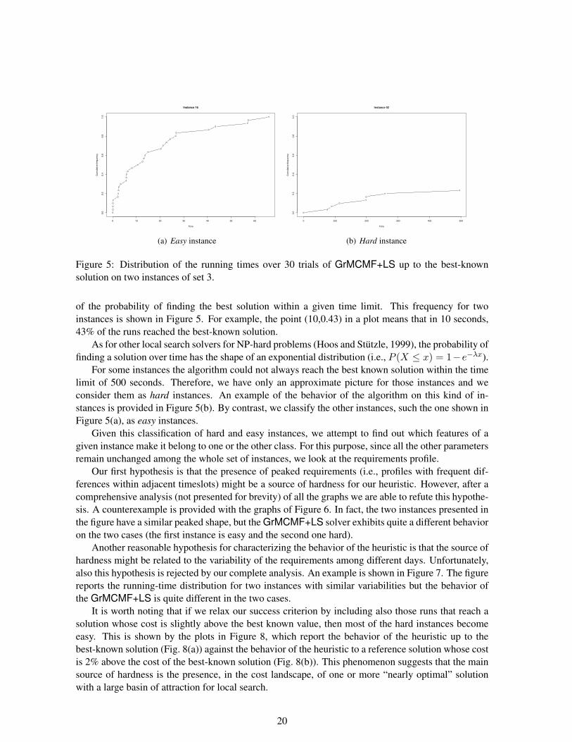
Figure 5: Distribution of the running times over 30 trials of GrMCMF+LS up to the best-knownsolution on two instances of set 3.

of the probability of finding the best solution within a given time limit. This frequency for twoinstances is shown in Figure 5. For example, the point (10,0.43) in a plot means that in 10 seconds,43% of the runs reached the best-known solution.

As for other local search solvers for NP-hard problems (Hoos and Stutzle, 1999), the probability offinding a solution over time has the shape of an exponential distribution (i.e., P (X ≤ x) = 1−e−λx).

For some instances the algorithm could not always reach the best known solution within the timelimit of 500 seconds. Therefore, we have only an approximate picture for those instances and weconsider them as hard instances. An example of the behavior of the algorithm on this kind of in-stances is provided in Figure 5(b). By contrast, we classify the other instances, such the one shown inFigure 5(a), as easy instances.

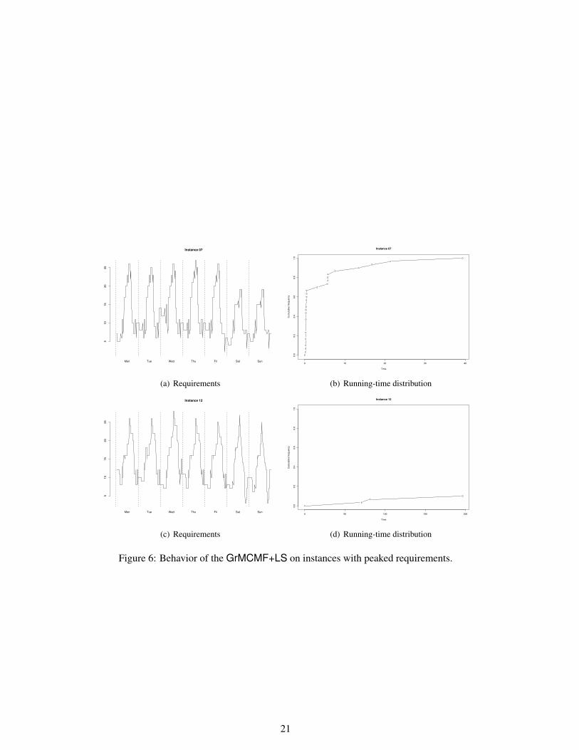
Given this classification of hard and easy instances, we attempt to find out which features of agiven instance make it belong to one or the other class. For this purpose, since all the other parametersremain unchanged among the whole set of instances, we look at the requirements profile.

Our first hypothesis is that the presence of peaked requirements (i.e., profiles with frequent dif-ferences within adjacent timeslots) might be a source of hardness for our heuristic. However, after acomprehensive analysis (not presented for brevity) of all the graphs we are able to refute this hypothe-sis. A counterexample is provided with the graphs of Figure 6. In fact, the two instances presented inthe figure have a similar peaked shape, but the GrMCMF+LS solver exhibits quite a different behavioron the two cases (the first instance is easy and the second one hard).

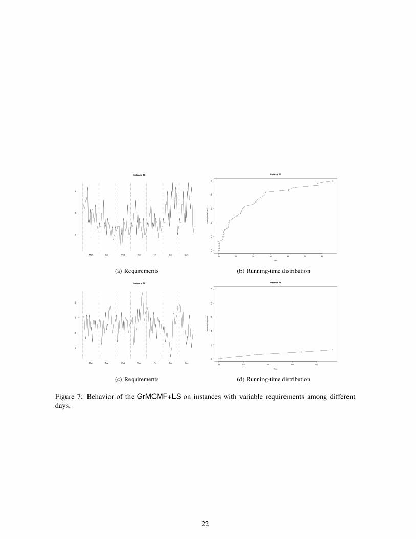
Another reasonable hypothesis for characterizing the behavior of the heuristic is that the source ofhardness might be related to the variability of the requirements among different days. Unfortunately,also this hypothesis is rejected by our complete analysis. An example is shown in Figure 7. The figurereports the running-time distribution for two instances with similar variabilities but the behavior ofthe GrMCMF+LS is quite different in the two cases.

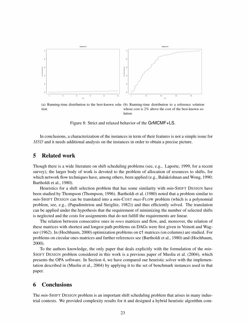
It is worth noting that if we relax our success criterion by including also those runs that reach asolution whose cost is slightly above the best known value, then most of the hard instances becomeeasy. This is shown by the plots in Figure 8, which report the behavior of the heuristic up to thebest-known solution (Fig. 8(a)) against the behavior of the heuristic to a reference solution whose costis 2% above the cost of the best-known solution (Fig. 8(b)). This phenomenon suggests that the mainsource of hardness is the presence, in the cost landscape, of one or more “nearly optimal” solutionwith a large basin of attraction for local search.

20

Mon Tue Wed Thu Fri Sat Sun

510

1520

25

Instance 07

(a) Requirements

0 10 20 30 40

0.0

0.2

0.4

0.6

0.8

1.0

Instance 07

Time

Cum

ulat

ive

frequ

ency

(b) Running-time distribution

Mon Tue Wed Thu Fri Sat Sun

510

1520

25

Instance 12

(c) Requirements

0 50 100 150 200

0.0

0.2

0.4

0.6

0.8

1.0

Instance 12

Time

Cum

ulat

ive

frequ

ency

(d) Running-time distribution

Figure 6: Behavior of the GrMCMF+LS on instances with peaked requirements.

21

Mon Tue Wed Thu Fri Sat Sun

1015

20

Instance 16

(a) Requirements

0 10 20 30 40 50 60

0.0

0.2

0.4

0.6

0.8

1.0

Instance 16

Time

Cum

ulat

ive

frequ

ency

(b) Running-time distribution

Mon Tue Wed Thu Fri Sat Sun

1015

2025

Instance 28

(c) Requirements

0 100 200 300 400

0.0

0.2

0.4

0.6

0.8

1.0

Instance 28

Time

Cum

ulat

ive

frequ

ency

(d) Running-time distribution

Figure 7: Behavior of the GrMCMF+LS on instances with variable requirements among differentdays.

22

0 20 40 60 80 100

0.0

0.2

0.4

0.6

0.8

1.0

Instance 19

Time

Cum

ulat

ive

frequ

ency

(a) Running-time distribution to the best-known solu-tion

0 100 200 300 400

0.0

0.2

0.4

0.6

0.8

1.0

Instance 19

Time

Cum

ulat

ive

frequ

ency

(b) Running-time distribution to a reference solutionwhose cost is 2% above the cost of the best-known so-lution

Figure 8: Strict and relaxed behavior of the GrMCMF+LS.

In conclusions, a characterization of the instances in term of their features is not a simple issue forMSD and it needs additional analysis on the instances in order to obtain a precise picture.

5 Related work

Though there is a wide literature on shift scheduling problems (see, e.g., Laporte, 1999, for a recentsurvey), the larger body of work is devoted to the problem of allocation of resources to shifts, forwhich network flow techniques have, among others, been applied (e.g., Balakrishnan and Wong, 1990;Bartholdi et al., 1980).

Heuristics for a shift selection problem that has some similarity with min-SHIFT DESIGN havebeen studied by Thompson (Thompson, 1996). Bartholdi et al. (1980) noted that a problem similar tomin-SHIFT DESIGN can be translated into a min-COST max-FLOW problem (which is a polynomialproblem, see, e.g., (Papadimitriou and Steiglitz, 1982)) and thus efficiently solved. The translationcan be applied under the hypothesis that the requirement of minimizing the number of selected shiftsis neglected and the costs for assignments that do not fulfill the requirements are linear.

The relation between consecutive ones in rows matrices and flow, and, moreover, the relation ofthese matrices with shortest and longest path problems on DAGs were first given in Veinott and Wag-ner (1962). In (Hochbaum, 2000) optimization problems on c1 matrices (on columns) are studied. Forproblems on circular ones matrices and further references see (Bartholdi et al., 1980) and (Hochbaum,2000).

To the authors knowledge, the only paper that deals explicitly with the formulation of the min-SHIFT DESIGN problem considered in this work is a previous paper of Musliu et al. (2004), whichpresents the OPA software. In Section 4, we have compared our heuristic solver with the implemen-tation described in (Musliu et al., 2004) by applying it to the set of benchmark instances used in thatpaper.

6 Conclusions

The min-SHIFT DESIGN problem is an important shift scheduling problem that arises in many indus-trial contexts. We provided complexity results for it and designed a hybrid heuristic algorithm com-

23

posed of a constructive heuristic (suggested by the complexity analysis) and a multi-neighborhoodtabu search procedure.

This problem appears to be quite difficult in practice, even for small instances, which is alsosupported by the theoretical results. An important source of hardness is related to the variability in thesize of the solution, since dropping this requirement makes the problem solvable in polynomial time.

In the experimental part, the hybrid heuristic and its underlying components have been evaluatedboth in terms of ability to reach good solutions and in quality of solutions reached in fast runs. Theoutcomes of the comparison show that the hybrid heuristic combines the good features of its compo-nents. Indeed, it obtained the best performances in terms of solution quality (thanks to the increasedthoroughness allowed by tabu search) but with a lower impact on the overall running time. Further-more, we compare our heuristics with the results obtained with a commercial software as reportedin (Musliu et al., 2004). Our hybrid heuristic clearly outperforms this commercial implementation,and thus can be considered as the best general-purpose solver among the other heuristics that werecompared to it.

In practice, a number of further optimization criteria clutters the problem, e.g., the average numberof working days per week. This number is an extremely good indicator with respect to how difficultit will be to develop a schedule and what quality that schedule will have. The average number ofduties thereby becomes the key criterion for working conditions and is sometimes even part of collec-tive agreements. Fortunately, this and most further criteria can easily be handled by straightforwardextensions of the heuristics described in this paper and add nothing to the complexity of MSD . Wetherefore concentrate on the three main criteria described in this paper.

7 Further ideas

The GreedyMCMF heuristic could be made even more efficient by noting that usually only veryfew edges change from one call to the next call of the MCMF() subroutine. We currently call theMCMF() subroutine each time from scratch. However, CS2 (Goldberg, 1997) supports a variant thatrecomputes an optimal flow more efficiently after a change in costs. It might thus prove worthwhileto track changes in the flow instance and recompute only those parts that are necessary, thus speedingup the MCMF() calls in the heuristics.

An idea for a promising heuristic might also be to integrate the MCMF() subroutine more directlyin the local search procedure instead of just calling them serially one after the other as in the thirdvariant of our heuristics.

Another simple heuristic that suggests itself might be to combine the MCMF() subroutine (to-gether with the postprocessing step described in Section 3.1 that reestablishes cyclicity) with a geneticalgorithm type of optimization heuristic. Indeed, the genetic code could consist merely of a bitvectorof all possible shifts, possibly ordered by their starting times. The phenotype would then consist ofthe shifts and number of staff as computed by the MCMF() subroutine followed by the postprocessingstep, applied only to the subset of shifts that have their bits set to 1. Optimization could then be donewith the usual crossover and mutation operators on populations of solution candidates, with selectionbeing based probabilistically on the scores of the phenotype solution candidates. Initial populationscould contain random bitvectors as well as shifts selected by single runs of the heuristics described inthis paper.

We also tried to apply PPRN3, a library for nonlinar network flow problems described in (Castroand Nabona, 1996) to our instances instead of calling MCMF but got only unsatisfactory results as

3http://www-eio.upc.es/∼jcastro/pprn.html

24

this package cannot correctly deal with fixed charge style nonlinearities. Other software specializingon MECF type problems or aiming at more general integer constraint problems might yield betterresults.

Acknowledgments: This work was supported by Austrian Science Fund Project No. Z29-N04 andby the Italian Ministry of Education, University and Research (MIUR) under the project PRIN 2003“Design and implementation of a solver based on local search for the execution of declarative speci-fications for combinatorial problems”.

References

Aarts, E. and Lenstra, J. K., editors (1997). Local Search in Combinatorial Optimization. John Wiley& Sons, New York (USA).

Ahuja, R., Magnanti, T., and Orlin, J. (1993). Network Flows. Prentice Hall, Englewood Cliffs (NJ,USA).

Balakrishnan, N. and Wong, R. (1990). A network model for the rotating workforce schedulingproblem. Networks, 20:25–42.

Bar-Ilan, J., Kortsarz, G., and Peleg, D. (2001). Generalized submodular cover problems and applica-tions. Theoretical Computer Science, 250(1–2):179–200.

Bartholdi, J., Orlin, J., and H.Ratliff (1980). Cyclic scheduling via integer programs with circularones. Operations Research, 28:110–118.

Burke, E. K., Causmaeker, P. D., Berghe, G. V., and Landeghem, H. V. (2004). The state of the art ofnurse rostering. Journal of Scheduling, 7:441–499.

Castro, J. and Nabona, N. (1996). An implementation of linear and nonlinear multicommodity net-work flows. European Journal of Operational Research, 92:37–53.

Di Gaspero, L. and Schaerf, A. (2003a). Multi-neighbourhood local search with application to coursetimetabling. In Burke, E. and Causmaecker, P. D., editors, Lecture Notes in Computer Science,number 2740 in Lecture Notes in Computer Science, pages 263–278. Springer-Verlag, Berlin-Heidelberg (Germany).

Di Gaspero, L. and Schaerf, A. (2003b). EASYLOCAL++: An object-oriented framework for flexibledesign of local search algorithms. Software Practice & Experience, 33(8):733–765.

Garey, M. R. and Johnson, D. S. (1979). Computers and Intractability—A guide to NP-completeness.W.H. Freeman and Company, San Francisco.

Gartner, J., Musliu, N., and Slany, W. (2001). Rota: a research project on algorithms for workforcescheduling and shift design optimization. AI Communications: The European Journal on ArtificialIntelligence, 14(2):83–92.

Glover, F. and Laguna, M. (1997). Tabu search. Kluwer Academic Publishers, Dordrecht (the Nether-lands).

25

Glover, F. and McMillan, C. (1986). The general employee scheduling problem: An integration ofMS and AI. Computers & Operations Research, 13(5):563–573.

Goldberg, A. (1997). An efficient implementation of a scaling minimum-cost flow algorithm. Journalof Algorithms, 22:1–29.

Hochbaum, D. (2000). Optimization over consecutive 1’s and circular 1’s constraints. Unpublishedmanuscript.

Hoos, H. H. and Stutzle, T. (1999). Towards a characterisation of the behaviour of stochastic localsearch algorithms for SAT. Artificial Intelligence, 112:213–232.

Hoos, H. H. and Stutzle, T. (2005). Stochastic Local Search: foundations and applications. MorganKaufmann, San Francisco (CA), USA.

Jackson, W., Havens, W., and Dollard, H. (1997). Staff scheduling: A simple approach that worked.Technical Report CMPT97-23, Intelligent Systems Lab, Centre for Systems Science, Simon FraserUniversity. Available at http://citeseer.nj.nec.com/101034.html.

Johnson, D. S. (2002). A theoretician’s guide to the experimental analysis of algorithms. In Gold-wasser, M. H., Johnson, D. S., and McGeoch, C. C., editors, Data Structures, Near NeighborSearches, and Methodology: Fifth and Sixth DIMACS Implementation Challenges, pages 215–250.American Mathematical Society.

Krumke, S., Noltemeier, H., Schwarz, S., Wirth, H.-C., and Ravi, R. (1998). Flow improvementand network flows with fixed costs. In Proceedings of the International Conference on OperationsResearch (OR-98), Zurich (Switzerland).

Laporte, G. (1999). The art and science of designing rotating schedules. Journal of the OperationalResearch Society, 50:1011–1017.

Lau, H. (1996). On the complexity of manpower scheduling. Computers & Operations Research,23(1):93–102.

Musliu, N., Gartner, J., and Slany, W. (2002). Efficient generation of rotating workforce schedules.Discrete Applied Mathematics, 118(1–2):85–98.

Musliu, N., Schaerf, A., and Slany, W. (2004). Local search for shift design. European Journal ofOperational Research, 153(1):51–64.

Papadimitriou, C. and Steiglitz, K. (1982). Combinatorial Optimization: Algorithms and Complexity.Prentice-Hall, Englewood Cliffs (NJ, USA).

Raz, R. and Safra, S. (1997). A sub constant error probability low degree test, and a sub constant errorprobability PCP characterization of NP. In Proceedings of the 29th ACM Symposium on Theory ofComputing, pages 475–484, El Paso (Texas, USA).

Thompson, G. (1996). A simulated-annealing heuristic for shift scheduling using non-continuouslyavailable employees. Computers & Operations Research, 23(3):275–278.

Tien, J. and Kamiyama, A. (1982). On manpower scheduling algorithms. SIAM Review, 24(3):275–287.

26

Veinott, A. and Wagner, H. (1962). Optimal capacity scheduling: Parts I and II. Operation Research,10:518–547.

27