Approximate Jacobian Matrices for Nonsmooth Continuous Maps and C 1 -Optimization

APPROXIMATE JACOBIAN MATRICES FOR NONSMOOTHCONTINUOUS MAPS AND C1-OPTIMIZATION∗

V. JEYAKUMAR† AND D. T. LUC‡

SIAM J. CONTROL OPTIM. c© 1998 Society for Industrial and Applied MathematicsVol. 36, No. 5, pp. 1815–1832, September 1998 013

Abstract. The notion of approximate Jacobian matrices is introduced for a continuous vector-valued map. It is shown, for instance, that the Clarke generalized Jacobian is an approximateJacobian for a locally Lipschitz map. The approach is based on the idea of convexificators of real-valued functions. Mean value conditions for continuous vector-valued maps and Taylor’s expansionsfor continuously Gateaux differentiable functions (i.e., C1-functions) are presented in terms of ap-proximate Jacobians and approximate Hessians, respectively. Second-order necessary and sufficientconditions for optimality and convexity of C1-functions are also given.

Key words. generalized Jacobians, nonsmooth analysis, mean value conditions, optimalityconditions

AMS subject classifications. 49A52, 90C30, 26A24

PII. S0363012996311745

1. Introduction. Over the past two decades, a great deal of research has focusedon the study of first- and second-order analysis of real-valued nonsmooth functions[2, 3, 4, 5, 11, 12, 14, 15, 21, 23, 24, 20, 25, 27, 28, 29, 30, 34, 35]. The results ofnonsmooth analysis of real-valued functions now provide basic tools of modern analysisin many branches of mathematics, such as mathematical programming, control, andmechanics. Indeed, the range of applications of nonsmooth calculus demonstrates itsbasic nature of nonsmooth phenomena in the mathematical and engineering sciences.

On the other hand, research in the area of nonsmooth analysis of vector-valuedmaps has been of substantial interest in recent years [2, 6, 7, 8, 9, 10, 18, 21, 22, 23,24, 29, 31]. In particular, it is known that the development and analysis of generalizedJacobian matrices for nonsmooth vector-valued maps are crucial from the viewpointof control problems and numerical methods of optimization. For instance, the Clarkegeneralized Jacobian matrices [2] of a locally Lipschitz map play an important role inthe Newton-based numerical methods for solving nonsmooth equations and optimiza-tion problems (see [26] and other references therein, and see also [17, 18, 19] for otherapplications). Warga [32, 33] examined derivative (unbounded derivative) containersin the context of local and global inverse function theorems as set-valued derivativesfor locally Lipschitz (continuous) vector-valued maps. Mordukhovich [21, 22] devel-oped generalized differential calculus for general nonsmooth vector-valued maps usingthe set-valued derivatives, called coderivatives [9, 21].

Our aim in this paper is to introduce a new concept of approximate Jacobianmatrices for continuous vector-valued maps that are not necessarily locally Lipschitz,develop certain calculus rules for approximate Jacobians, and apply the concept tooptimization problems involving continuously Gateaux differentiable functions. This

∗Received by the editors November 8, 1996; accepted for publication (in revised form) October 2,1997; published electronically July 9, 1998. This research was partially supported by a grant fromthe Australian Research Council.

http://www.siam.org/journals/sicon/36-5/31174.html†Department of Applied Mathematics, University of New South Wales, Sydney 2052, Australia

([email protected]). Some of the work of this author was carried out while visiting the Centrefor Experimental and Constructive Mathematics at the Simon Fraser University, Canada.‡Institute for Mathematics, Hanoi, Vietnam ([email protected]). Some of the work of this

author was done while visiting the University of New South Wales.

1815

Dow

nloa

ded

09/2

6/14

to 1

30.6

4.11

.153

. Red

istr

ibut

ion

subj

ect t

o SI

AM

lice

nse

or c

opyr

ight

; see

http

://w

ww

.sia

m.o

rg/jo

urna

ls/o

jsa.

php

1816 V. JEYAKUMAR AND D. T. LUC

concept is a generalization of the idea of convexificators of real-valued functions,studied recently in [4, 5, 13], to vector-valued maps. Convexificators provide two-sided convex approximations [30] for real-valued functions. Unlike the set-valuedgeneralized derivatives [9, 21, 22, 32, 33], mentioned above for vector-valued maps,the approximate Jacobian is defined as a closed subset of the space of (n×m) matricesfor a vector-valued map from Rn into Rm.

Approximate Jacobians not only extend the nonsmooth analysis of locally Lip-schitz maps to continuous maps but also unify and strengthen various results ofnonsmooth analysis. They also enjoy useful calculus, such as the generalized meanvalue property and chain rules. Moreover, approximate Jacobians allow us to presentsecond-order optimality conditions in easily verifiable forms in terms of approximateHessian matrices for C1-optimization problems, extending the corresponding resultsfor C1,1-problems [7].

The outline of the paper is as follows. In section 2, approximate Jacobian ma-trices are introduced, and it is shown that for a locally Lipschitz map the Clarkegeneralized Jacobian is an approximate Jacobian. Various examples of approximateJacobians are also given. Section 3 establishes mean value conditions for continuousvector-valued maps and provides necessary and sufficient conditions in terms of ap-proximate Jacobians for a continuous map to be locally Lipschitz. Various calculusrules for approximate Jacobians are given in section 4. Approximate Hessian matri-ces are introduced in section 5, and their connections to C1,1-functions are discussed.Section 6 presents generalizations of Taylor’s expansions for C1-functions. In section7, second-order necessary and sufficient conditions for optimality and convexity ofC1-functions are given.

2. Approximate Jacobians for continuous maps. This section contains no-tation, definitions, and preliminaries that will be used throughout the paper. LetF : Rn → Rm be a continuous function which has components (f1, . . . , fm). For eachv ∈ Rm, the composite function, (vF ) : Rn → R, is defined by

(vF )(x) = 〈v, F (x)〉 =m∑i=1

vifi(x).

The lower Dini directional derivative and the upper Dini directional derivative of vFat x in the direction u ∈ Rn are defined by

(vF )−(x, u) := lim inft↓0

(vF )(x+ tu)− (vF )(x)

t,

(vF )+(x, u) := lim supt↓0

(vF )(x+ tu)− (vF )(x)

t.

We denote by L(Rn,Rm) the space of all (n×m) matrices. The convex hull and theclosed convex hull of a set A in a topological vector space are denoted by co(A) andco(A), respectively.

Definition 2.1. The map F : Rn → Rm admits an approximate Jacobian∂∗F (x) at x ∈ Rn if ∂∗F (x) ⊆ L(Rn,Rm) is closed, and for each v ∈ Rm,

(2.1) (vF )−(x, u) ≤ supM∈∂∗F (x)

〈Mv, u〉 ∀u ∈ Rn.Dow

nloa

ded

09/2

6/14

to 1

30.6

4.11

.153

. Red

istr

ibut

ion

subj

ect t

o SI

AM

lice

nse

or c

opyr

ight

; see

http

://w

ww

.sia

m.o

rg/jo

urna

ls/o

jsa.

php

APPROXIMATE JACOBIANS AND OPTIMIZATION 1817

A matrix M of ∂∗F (x) is called an approximate Jacobian matrix of F at x. Notethat condition (2.1) is equivalent to the condition

(2.2) (vF )+(x, u) ≥ infM∈∂∗F (x)

〈Mv, u〉 ∀u ∈ Rn.

It is worth noting that the inequality (2.1) means that the set ∂∗F (x)v is an upperconvexificator [13, 16] of the function vF at x. Similarly, the inequality (2.2) statesthat ∂∗F (x)v is a lower convexificator of vF at x. In the case m = 1, the inequality(2.1) (or (2.2)) is equivalent to the condition

(2.3) F−(x, u) ≤ supx∗∈∂∗F (x)

〈x∗, u〉 and F+(x, u) ≥ infx∗∈∂∗F (x)

〈x∗, u〉;

thus, the set ∂∗F (x) is a convexificator of F at x. Also note that in the case m = 1,condition (2.3) is also equivalent to the condition that for each α ∈ R,

(2.4) (αF )−(x, u) ≤ supx∗∈∂∗F (x)

〈αx∗, u〉 ∀u ∈ Rn.

Similarly, the condition (2.3) is also equivalent to the condition that for each α ∈ R,

(2.5) (αF )+(x, u) ≥ infx∗∈∂∗F (x)

〈αx∗, u〉 ∀u ∈ Rn.

For applications of convexificators, see [5, 13, 16]. To clarify the definition, let usconsider some examples.

Example 2.2. If F : Rn → Rm is continuously differentiable at x, then any closedsubset Φ(x) of L(Rn,Rm) containing the Jacobian ∇F (x) is an approximate Jacobianof F at x. In this case, for each v ∈ Rm,

(vF )−(x, u) = 〈∇F (x)v, u〉 ≤ supM∈Φ(x)

〈Mv, u〉 ∀u ∈ Rn.

Observe from the definition of the approximate Jacobian that for any map F : Rn →Rm, the whole space L(Rn,Rm) serves as a trivial approximate Jacobian for F at anypoint in Rn. Let us now examine approximate Jacobians for locally Lipschitz maps.

Example 2.3. Suppose that F : Rn → Rm is locally Lipschitz at x. Then theClarke generalized Jacobian ∂CF (x) is an approximate Jacobian of F at x. Indeed,for each v ∈ Rm,

(2.6) ∂(vF )(x) = ∂CF (x)v.

Consequently, for each u ∈ Rn,

(vF )(x, u) = maxξ∈∂(vF )(x)

〈ξ, u〉 = maxM∈∂CF (x)

〈Mv, u〉,

where

∂CF (x) = co limn→∞∇F (xn)T : xn ∈ Ω, xn → x,

Ω is the set of points in Rn where F is differentiable, and the Clarke directionalderivative of vF is given by

(vF )(x, u) = lim supx′→xt↓0

〈v, F (x′ + tu)− F (x′)〉t

.

Dow

nloa

ded

09/2

6/14

to 1

30.6

4.11

.153

. Red

istr

ibut

ion

subj

ect t

o SI

AM

lice

nse

or c

opyr

ight

; see

http

://w

ww

.sia

m.o

rg/jo

urna

ls/o

jsa.

php


Since for each u ∈ Rn,

(vF )−(x, u) ≤ (vF )(x, u) ∀u ∈ Rn,

the set ∂CF (x) is an approximate Jacobian of F at x.For the locally Lipschitz map F : Rn → Rm, the set

∂BF (x) := limn→∞∇F (xn)T : xn ∈ Ω, xn → x

is also an approximate Jacobian of F at x. The set ∂BF (x) is known as the B-subdifferential of F at x, which plays a significant role in the development of nons-mooth Newton methods (see [26]). In passing, note that for each v ∈ Rm,

∂(vF )(x) = co(∂M (vF )(x)) = co(D∗F (x)(v)),

where the set-valued mapping D∗F (x) from Rm into Rn is the coderivative of F atx and ∂M (vF )(x) is the first-order subdifferential of vF at x in the sense of Mor-dukhovich [22]. However, for locally Lipschitz maps, the coderivative does not appearto have a representation of the form (2.6), which allowed us above to compare ap-proximate Jacobians with the Clarke generalized Jacobian. The reader is referred to[9, 21, 22, 29] for a more general definition and associated properties of coderivatives.A second-order analogue of the coderivative for vector-valued maps is given recentlyin [10].

Let us look at a numerical example of a locally Lipschitz map where the Clarkegeneralized Jacobian strictly contains an approximate Jacobian.

Example 2.4. Consider the function F : R2 → R2

F (x, y) = (|x|, |y|).

Then

∂∗F (0) =

(1 00 1

),

(1 00 −1

),

( −1 00 1

),

( −1 00 −1

)is an approximate Jacobian of F at 0. On the other hand, the Clarke generalizedJacobian

∂CF (0) =

(α 00 β

): α, β ∈ [−1, 1]

,

which is also an approximate Jacobian of F at 0 and contains ∂∗F (0).Observe in this example that ∂CF (0) is the convex hull of ∂∗F (0). However, this

is not always the case. The following example illustrates that even for the case wherem = 1, the convex hull of an approximate Jacobian of a locally Lipschitz map maybe strictly contained in the Clarke generalized Jacobian.

Example 2.5. Define F : R2 → R by

F (x, y) = |x| − |y|.

Then it can easily be verified that

∂∗1F (0) = (1, 1), (−1,−1) and ∂∗2F (0) = (1,−1), (−1, 1)

Dow

nloa

ded

09/2

6/14

to 1

30.6

4.11

.153

. Red

istr

ibut

ion

subj

ect t

o SI

AM

lice

nse

or c

opyr

ight

; see

http

://w

ww

.sia

m.o

rg/jo

urna

ls/o

jsa.

php


are approximate Jacobians of F at 0, whereas

∂BF (0) = (1, 1), (−1, 1), (1,−1), (−1,−1)and

∂CF (0) = co((1, 1), (−1, 1), (1,−1), (−1,−1)).It is also worth noting that

co(∂∗1F (0)) ⊂ co(∂MF (0)) = ∂CF (0).

Clearly, this example shows that certain results, such as mean value conditions andnecessary optimality conditions that are expressed in terms of ∂∗F (x), may providesharp conditions even for locally Lipschitz maps (see section 3).

Let us now present an example of a continuous map where the Clarke generalizedJacobian does not exist, whereas approximate Jacobians are quite easy to calculate.

Example 2.6. Define F : R2 → R2 by

F (x, y) = (√|x| sgn(x) + |y|,

√|y| sgn(y) + |y|),

where sgn(x) = 1 for x > 0, 0 for x = 0, and −1 for x < 0. Then F is not locallyLipschitz at (0, 0), and so the Clarke generalized Jacobian does not exist. However,for each c ∈ R, the set

∂∗F (0, 0) =

(α 10 β

),

(α −10 β

): α, β ≥ c

is an approximate Jacobian of F at (0, 0).

3. Generalized mean value theorems. In this section we derive mean valuetheorems for continuous maps in terms of approximate Jacobians and show how locallyLipschitz vector-valued maps can be characterized using approximate Jacobians.

Theorem 3.1. Let a, b ∈ Rn and F : Rn → Rm be continuous. Assume that foreach x ∈ [a, b], ∂∗F (x) is an approximate Jacobian of F at x. Then

F (b)− F (a) ∈ co(∂∗F ([a, b])(b− a)).

Proof. Let us first note that the right-hand side above is the closed convex hull ofall points of the form M(b− a), where M ∈ ∂∗F (ζ) for some ζ ∈ [a, b]. Let v ∈ Rmbearbitrary and fixed. Consider the real-valued function g : [0, 1]→ IR

g(t) = 〈v, F (a+ t(b− a))− F (a) + t(F (a)− F (b))〉.Then g is continuous on [0, 1] with g(0) = g(1). So g attains a minimum or a maximumat some t0 ∈ (0, 1). Suppose that t0 is a minimum point. Then, for each α ∈ R,g−(t0, α) ≥ 0. It now follows from direct calculations that

g−(t0, α) = (vF )−(a+ t0(b− a), α(b− a)) + α〈v, F (a)− F (b)〉.Hence, for each α ∈ R,

(vF )−(a+ t0(b− a), α(b− a)) ≥ α〈v, F (b)− F (a)〉.

Dow

nloa

ded

09/2

6/14

to 1

30.6

4.11

.153

. Red

istr

ibut

ion

subj

ect t

o SI

AM

lice

nse

or c

opyr

ight

; see

http

://w

ww

.sia

m.o

rg/jo

urna

ls/o

jsa.

php


Now, by taking α = 1 and α = −1, we obtain that

−(vF )−(a+ t0(b− a), a− b) ≤ 〈v, F (b)− F (a)〉 ≤ (vF )−(a+ t0(b− a), b− a)〉.

By (2.1), we get

infM∈∂∗F (a+t0(b−a))

〈Mv, b− a〉 ≤ 〈v, F (b)− F (a)〉 ≤ supM∈∂∗F (a+t0(b−a))

〈Mv, b− a〉.

Consequently,

〈v, F (b)− F (a)〉 ∈ co(∂∗F (a+ t0(b− a))v)(b− a),

and so

(3.1) 〈v, F (b)− F (a)〉 ∈ co(∂∗F ([a, b])v)(b− a).

Since this inclusion holds for each v ∈ Rm, we claim that

F (b)− F (a) ∈ co(∂∗F ([a, b])(b− a)).

If this is not so, then it follows from the separation theorem

〈p, F (b)− F (a)〉 − ε > supu∈co(∂∗F ([a,b])(b−a))

〈p, u〉

for some p ∈ Rm since co(∂∗F ([a, b])(b − a)) is a closed convex subset of Rm. Thisimplies

〈p, F (b)− F (a)〉 > supα : α ∈ co(∂∗F ([a, b])p)(b− a),

which contradicts (3.1).Similarly, if t0 is a maximum point, then g+(t0, α) ≤ 0 for each α ∈ R. Using the

same line of arguments as above, we arrive at the same conclusion, and so the proofis complete.

Corollary 3.2. Let a, b ∈ Rn and F : Rn → Rm be continuous. Assume that∂∗F (x) is a bounded approximate Jacobian of F at x for each x ∈ [a, b]. Then

(3.2) F (b)− F (a) ∈ co(∂∗F ([a, b])(b− a)).

Proof. Since for each x ∈ [a, b], ∂∗F (x) is compact, the set

co(∂∗F ([a, b])(b− a) = co∂∗F ([a, b])(b− a)

is closed, and so the conclusion follows from Theorem 3.1.In the following corollary we deduce the mean value theorem for locally Lipschitz

maps (see [1, 6]) as a special case of Theorem 3.1.Corollary 3.3. Let a, b ∈ Rn and F : Rn → Rm be locally Lipschitz on Rn.

Then

(3.3) F (b)− F (a) ∈ co(∂CF ([a, b])(b− a)).Dow

nloa

ded

09/2

6/14

to 1

30.6

4.11

.153

. Red

istr

ibut

ion

subj

ect t

o SI

AM

lice

nse

or c

opyr

ight

; see

http

://w

ww

.sia

m.o

rg/jo

urna

ls/o

jsa.

php


Proof. In this case the Clarke generalized Jacobian ∂CF (x) is a convex and com-pact approximate Jacobian of F at x. Hence, the conclusion follows from Corollary3.2.

Note that even for the case where F is locally Lipschitz, Corollary 3.2 provides astronger mean value condition than condition (3.3) of Corollary 3.3. To see this, letn = 2, m = 1, F (x, y) = |x| − |y|, a = (−1,−1), and b = (1, 1). Then condition (3.2)of Corollary 3.2 is verified by

∂∗F (0) = (1,−1), (−1, 1).

However, condition (3.3) holds for ∂CF (0), where

∂CF (0) = co((1, 1), (−1,−1), (1,−1), (−1, 1)) ⊃ ∂∗F (0).

As a special case of the above theorem, we see that if F is real-valued, then anasymptotic mean value equality is obtained. This was shown in [13].

Corollary 3.4. Let a, b ∈ X and F : Rn → R be continuous. Assume that,for each x ∈ [a, b], ∂∗F (x) is a convexificator of F . Then there exist c ∈ (a, b) and asequence x∗k ⊂ co(∂∗F (c)) such that

F (b)− F (a) = limk→∞

〈x∗k, b− a〉.

Proof. The conclusion follows from the proof of Theorem 3.1 by noting that aconvexificator ∂∗F (x) is an approximate Jacobian of F at x.

We now see how locally Lipschitz functions can be characterized using the abovemean value theorem. We say that a set-valued mapping G : Rn → L(Rn,Rm) is locallybounded at x if there exist a neighborhood U of x and a positive α such that ||A|| ≤ αfor each A ∈ G(U). Recall that the map G is said to be upper semicontinuous atx if for each open set V containing G(x) there is a neighborhood U of x such thatG(U) ⊂ V . Clearly, if G is upper semicontinuous at x and if G(x) is bounded, then Gis locally bounded at x.

Theorem 3.5. Let F : Rn → Rm be continuous. Then F has a locally boundedapproximate Jacobian map ∂∗F at x if and only if F is locally Lipschitz at x.

Proof. Assume that ∂∗F (y) is the approximate Jacobian of F for each y in aneighborhood U of x and that ∂∗F is locally bounded on U . Without loss of generality,we may assume that U is convex. Then there exists α > 0 such that ||A|| ≤ α foreach A ∈ ∂∗F (U). Let x, y ∈ U . Then [x, y] ⊂ U , and by the mean value theorem,

F (x)− F (y) ∈ co(∂∗F ([x, y])(x− y)) ⊂ co(∂∗F (U)(x− y)).

Hence,

‖F (x)− F (y)‖ ≤ ‖x− y‖max‖A‖ : A ∈ ∂∗F (U).

This gives us that

‖F (x)− F (y)‖ ≤ α‖x− y‖,

and so F is locally Lipschitz at x.Conversely, if F is locally Lipschitz at x, then the Clarke generalized Jacobian

can be chosen as an approximate Jacobian for F , which is locally bounded at x.

Dow

nloa

ded

09/2

6/14

to 1

30.6

4.11

.153

. Red

istr

ibut

ion

subj

ect t

o SI

AM

lice

nse

or c

opyr

ight

; see

http

://w

ww

.sia

m.o

rg/jo

urna

ls/o

jsa.

php


4. Calculus rules for approximate Jacobians. In this section, we presentsome basic calculus rules for approximate Jacobians. We begin by introducing thenotion of regular approximate Jacobians which are useful in some applications.

Definition 4.1. The map F : Rn → Rm admits a regular approximate Jacobian,∂∗F (x) at x ∈ Rn if ∂∗F (x) ⊆ L(Rn,Rm) is closed, and for each v ∈ Rm,

(4.1) (vF )+(x, u) = supM∈∂∗F (x)

〈Mv, u〉 ∀u ∈ Rn,

or equivalently,

(4.2) (vF )−(x, u) = infM∈∂∗F (x)

〈Mv, u〉 ∀u ∈ Rn.

Note that in the case m = 1, this definition collapses to the notion of the regularconvexificator studied in [13]. Thus, a closed set ∂∗h(x) ⊂ Rn is a regular convexifi-cator of the real-valued function h at x if for each u ∈ Rn,

h−(x, u) = infξ∈∂∗h(x)

〈ξ, u〉 and h+(x, u) = supξ∈∂∗h(x)

〈ξ, u〉.

It is evident that these equalities follow from (4.1) by taking F = h and v = −1 andv = 1, respectively.

It is immediate from the definition that if F is differentiable at x, then ∇f(x)is a regular approximate Jacobian of F at x. However, if F is locally Lipschitz at x,then the Clarke generalized Jacobian ∂CF (x) is not necessarily a regular approximateJacobian of F at x. It is also worth noting that if ∂∗1F (x) and ∂∗2F (x) are two regularapproximate Jacobians of F at x, then co(∂∗1F (x)) = co(∂∗2F (x)).

In passing, we note that if F is locally Lipschitz on a neighborhood U of x, thenthere exists a dense set K ⊂ U such that F admits a regular approximate Jacobianat each point of K. By Rademacher’s theorem, the dense subset can be chosen as theset where F is differentiable.

Theorem 4.2 (Rule 1). Let F and H be continuous maps from Rn to Rm.Assume that ∂∗F (x) is an approximate Jacobian of F at x and ∂∗H(x) is a regularapproximate Jacobian of H at x. Then the set ∂∗F (x) + ∂∗H(x) is an approximateJacobian of F +H at x.

Proof. Let v ∈ Rm, u ∈ Rn be arbitrary. By definition,

〈v, F +H〉−(x, u) = lim inft↓0

〈v, F (x+ tu)− F (x) +H(x+ tu)−H(x)〉t

.

Let tn be a sequence of positive numbers converging to 0 such that

〈v, F +H〉−(x, u) = limn→∞

〈v, F (x+ tnu)− F (x) +H(x+ tnu)−H(x)〉tn

.

Further, let sn be another sequence of positive numbers converging to 0 such that

〈v, F 〉−(x, u) = lim inft↓0

〈v, F (x+ tu)− F (x)〉t

= limn→∞

〈v, F (x+ snu)− F (x)〉sn

.

Then we have

limn→∞


≤ supM∈∂∗F (x)

〈Mv, u〉Dow

nloa

ded

09/2

6/14

to 1

30.6

4.11

.153

. Red

istr

ibut

ion

subj

ect t

o SI

AM

lice

nse

or c

opyr

ight

; see

http

://w

ww

.sia

m.o

rg/jo

urna

ls/o

jsa.

php


and

lim supn→∞

〈v,H(x+ snu)−H(x)〉sn

≤ 〈v,H〉+(x, u) = supM∈∂∗H(x)

〈Mv, u〉.

Consequently,

〈v, F +H〉−(x, u) ≤ limn→∞


+〈v,H(x+ snu)−H(x)〉

sn≤ supM∈∂∗F (x)

〈Mv, u〉+ supN∈∂∗H(x)

〈Nv, u〉

= supP∈∂∗F (x)+∂∗H(x)

〈Pv, u〉.

Since u and v are arbitrary, we conclude that ∂∗F (x) + ∂∗H(x) is an approximateJacobian of F +H at x.

Note that as in the case of convexificators of real-valued functions [18], the set∂∗F (x) + ∂∗H(x) is not necessarily regular at x.

Theorem 4.3 (Rule 2). Let F : Rn → Rm and H : IRm → Rl be continuousmaps. Assume that ∂∗F (x) is a bounded approximate Jacobian of F at x and ∂∗H(x)is a bounded approximate Jacobian of H at F (x). If the maps ∂∗F and ∂∗H are uppersemicontinuous at x and F (x), respectively, then ∂∗H(F (x))∂∗F (x) is an approximateJacobian of H F at x.

Proof. Let w ∈ Rl and u ∈ Rm be arbitrary. Consider the lower Dini directionalderivative of 〈w, H F 〉 at x:

〈w, H F 〉−(x, u) = lim inft↓0

〈w, H(F (x+ tu))−H(F (x))〉t

.

By applying the mean value theorem (see Theorem 3.1) to H and F , we obtain

F (x+ tu)− F (x) ∈ tco(∂∗F ([x, x+ tu])u),

H(F (x+ tu))−H(F (x)) ∈ co(∂∗H([F (x, ), F (x+ tu)])(F (x+ tu)− F (x)))

It now follows from the upper semicontinuity of ∂∗F and ∂∗H that for an arbitrarysmall positive ε we can find t0 > 0 such that for t ∈ (0, t0) we have

∂∗F ([x, x+ tu]) ⊆ ∂∗F (x) + εB1,

∂∗H([F (x), F (x+ tu)]) ⊆ ∂∗H(F (x)) + εB2,

where B1 and B2 are the unit balls in L(Rn,Rm) and L(Rm,Rl), respectively. Usingthese inclusions, we obtain

〈w, H(F (x+ tu))−H(F (x))〉t

∈ 〈w,A〉,where

A := co((∂∗H(F (x))∂∗F (x) + ε(∂∗H(F (x))B1 +B2∂∗F (x)) + ε2B2B1)u).

Since ∂∗H(F (x)) and ∂∗F (x) are bounded, we can find α > 0 such that ‖M‖ ≤ α forall M ∈ ∂∗H(F (x)) or M ∈ ∂∗F (x). Consequently,

〈w,H F 〉−(x, u) ≤ supM∈∂∗H(F (x))∂∗F (x)

〈Mw,u〉+ 2ε‖u‖+ ε2‖u|.

As ε is arbitrary, we conclude that ∂∗H(F (x))∂∗F (x) is an approximate Jacobian ofH F at x.

Dow

nloa

ded

09/2

6/14

to 1

30.6

4.11

.153

. Red

istr

ibut

ion

subj

ect t

o SI

AM

lice

nse

or c

opyr

ight

; see

http

://w

ww

.sia

m.o

rg/jo

urna

ls/o

jsa.

php


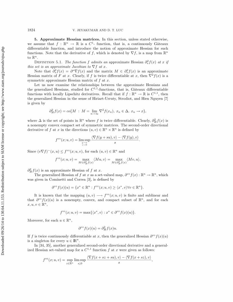
5. Approximate Hessian matrices. In this section, unless stated otherwise,we assume that f : Rn → R is a C1- function, that is, a continuously Gateauxdifferentiable function, and introduce the notion of approximate Hessian for suchfunctions. Note that the derivative of f , which is denoted by ∇f , is a map from Rnto Rn.

Definition 5.1. The function f admits an approximate Hessian ∂2∗f(x) at x if

this set is an approximate Jacobian to ∇f at x.Note that ∂2

∗f(x) = ∂∗∇f(x) and the matrix M ∈ ∂2∗f(x) is an approximate

Hessian matrix of F at x. Clearly, if f is twice differentiable at x, then ∇2f(x) is asymmetric approximate Hessian matrix of f at x.

Let us now examine the relationships between the approximate Hessians andthe generalized Hessians, studied for C1,1-functions, that is, Gateaux differentiablefunctions with locally Lipschitz derivatives. Recall that if f : Rn → R is C1,1, thenthe generalized Hessian in the sense of Hiriart-Urruty, Strodiot, and Hien Nguyen [7]is given by

∂2Hf(x) = coM : M = lim

n→∞∇2f(xn), xn ∈ ∆, xn → x,

where ∆ is the set of points in Rn where f is twice differentiable. Clearly, ∂2Hf(x) is

a nonempty convex compact set of symmetric matrices. The second-order directionalderivative of f at x in the directions (u, v) ∈ Rn × Rn is defined by

f(x;u, v) = lim supy→xs→0

〈∇f(y + su), v〉 − 〈∇f(y), v〉s

.

Since (v∇f)−(x, u) ≤ f(x;u, v), for each (u, v) ∈ Rn and

f(x;u, v) = maxM∈∂2

Hf(x)〈Mu, v〉 = max

M∈∂2Hf(x)〈Mv, u〉,

∂2Hf(x) is an approximate Hessian of f at x.

The generalized Hessian of f at x as a set-valued map, ∂f(x) : Rn → Rn, whichwas given in Cominetti and Correa [3], is defined by

∂f(x)(u) = x∗ ∈ Rn : f(x;u, v) ≥ 〈x∗, v〉∀v ∈ Rn.It is known that the mapping (u, v) −→ f(x;u, v) is finite and sublinear and

that ∂f(x)(u) is a nonempty, convex, and compact subset of Rn, and for eachx, u, v ∈ Rn,

f(x;u, v) = max〈x∗, v〉 : x∗ ∈ ∂f(x)(u).Moreover, for each u ∈ Rn,

∂f(x)(u) = ∂2Hf(x)u.

If f is twice continuously differentiable at x, then the generalized Hessian ∂f(x)(u)is a singleton for every u ∈ IRn.

In [34, 35], another generalized second-order directional derivative and a general-ized Hessian set-valued map for a C1,1 function f at x were given as follows:

f(x;u, v) = supz∈Rn

lim sups↓0

〈∇f(x+ sz + su), v〉 − 〈∇f(x+ sz), v〉s

,

Dow

nloa

ded

09/2

6/14

to 1

30.6

4.11

.153

. Red

istr

ibut

ion

subj

ect t

o SI

AM

lice

nse

or c

opyr

ight

; see

http

://w

ww

.sia

m.o

rg/jo

urna

ls/o

jsa.

php


∂f(x)(u) = x∗ ∈ X∗ : f(x;u, v) ≥ 〈x∗, v〉 ∀v ∈ X.It was shown that the mapping (u, v) −→ f(x;u, v) is finite and sublinear;

∂f(x)(u) is a nonempty, convex, and compact subset of Rn; and ∂f(x)(u) issingled-valued for each u ∈ IRn if and only if f is twice Gateaux differentiable at x.Further, for each u ∈ Rn, ∂f(x)(u) ⊂ ∂f(x)(u) = ∂2

Hf(x)u. If for each (u, v) ∈ Rnthe function y −→ f(y;u, v) is upper semicontinuous at x, then

∂f(x)(u) = ∂2Hf(x)u.

The following proposition gives us necessary and sufficient conditions in terms ofapproximate Hessians for a C1-function to be C1,1.

Proposition 5.2. Let f : Rn → R be a C1-function. Then f has a locallybounded approximate Hessian map ∂2

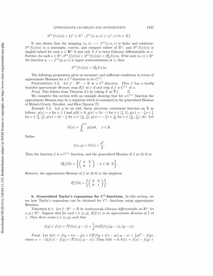
∗f at x if and only if f is C1,1 at x.Proof. This follows from Theorem 3.5 by taking F as ∇f .We complete this section with an example showing that for a C1,1 function the

approximate Hessian may be a singleton which is contained in the generalized Hessianof Hiriart-Urruty, Strodiot, and Hien Nguyen [7].

Example 5.3. Let g be an odd, linear piecewise continuous function on R asfollows. g(x) = x for x ≥ 1 and g(0) = 0; g(x) = 2x−1 for x ∈ [ 1

2 , 1]; g(x) = − 12x+ 1

4for x ∈ [ 1

6 ,12 ]; g(x) = 2x− 1

6 for x ∈ [ 112 ,

16 ]; g(x) = − 1

4x+ 148 for x ∈ [ 1

60 ,112 ], etc. Let

G(x) =

∫ |x|0

g(t)dt, x ∈ R.

Define

f(x, y) = G(x) +y2

2.

Then the function f is a C1,1 function, and the generalized Hessian of f at (0, 0) is

∂2Hf(0) =

(α 00 1

): α ∈ [0, 2]

.

However, the approximate Hessian of f at (0, 0) is the singleton

∂2∗f(0) =

(0 00 1

).

6. Generalized Taylor’s expansions for C1-functions. In this section, wesee how Taylor’s expansions can be obtained for C1- functions using approximateHessians.

Theorem 6.1. Let f : Rn → R be continuously Gateaux differentiable on Rn; letx, y ∈ Rn. Suppose that for each z ∈ [x, y], ∂2

∗f(z) is an approximate Hessian of f atz. Then there exists ζ ∈ (x, y) such that

f(y) ∈ f(x) + 〈∇f(x), y − x〉+1

2co〈∂2

∗f(ζ)(y − x), (y − x)〉.

Proof. Let h(t) = f(y + t(x − y)) + t〈∇f(y + t(x − y)), y − x〉 + 12at

2 − f(y),where a = −2(f(x) − f(y) + 〈∇f(x), y − x〉). Then h(0) = 0, h(1) = f(x) − f(y) +

Dow

nloa

ded

09/2

6/14

to 1

30.6

4.11

.153

. Red

istr

ibut

ion

subj

ect t

o SI

AM

lice

nse

or c

opyr

ight

; see

http

://w

ww

.sia

m.o

rg/jo

urna

ls/o

jsa.

php


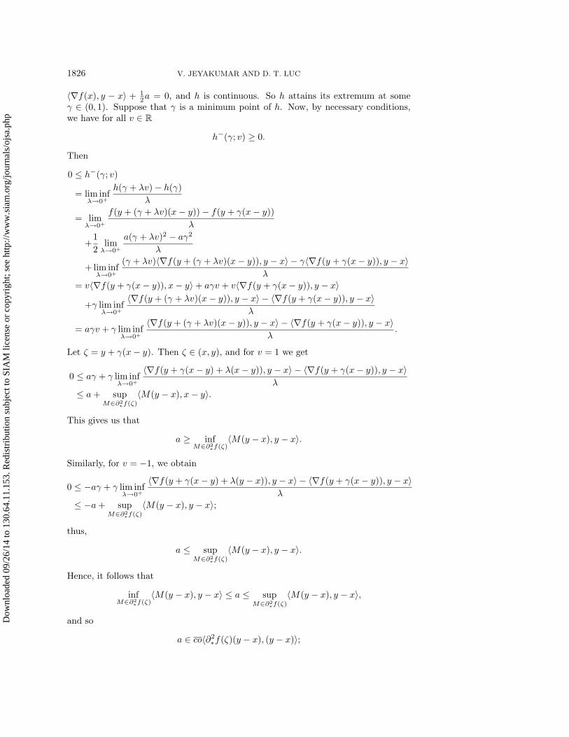
〈∇f(x), y − x〉 + 12a = 0, and h is continuous. So h attains its extremum at some

γ ∈ (0, 1). Suppose that γ is a minimum point of h. Now, by necessary conditions,we have for all v ∈ R

h−(γ; v) ≥ 0.

Then

0 ≤ h−(γ; v)

= lim infλ→0+

h(γ + λv)− h(γ)

λ

= limλ→0+

f(y + (γ + λv)(x− y))− f(y + γ(x− y))

λ

+1

2limλ→0+

a(γ + λv)2 − aγ2

λ

+ lim infλ→0+

(γ + λv)〈∇f(y + (γ + λv)(x− y)), y − x〉 − γ〈∇f(y + γ(x− y)), y − x〉λ

= v〈∇f(y + γ(x− y)), x− y〉+ aγv + v〈∇f(y + γ(x− y)), y − x〉+γ lim inf

λ→0+

〈∇f(y + (γ + λv)(x− y)), y − x〉 − 〈∇f(y + γ(x− y)), y − x〉λ

= aγv + γ lim infλ→0+

〈∇f(y + (γ + λv)(x− y)), y − x〉 − 〈∇f(y + γ(x− y)), y − x〉λ

.

Let ζ = y + γ(x− y). Then ζ ∈ (x, y), and for v = 1 we get

0 ≤ aγ + γ lim infλ→0+

〈∇f(y + γ(x− y) + λ(x− y)), y − x〉 − 〈∇f(y + γ(x− y)), y − x〉λ

≤ a+ supM∈∂2∗f(ζ)

〈M(y − x), x− y〉.

This gives us that

a ≥ infM∈∂2∗f(ζ)

〈M(y − x), y − x〉.

Similarly, for v = −1, we obtain

0 ≤ −aγ + γ lim infλ→0+

〈∇f(y + γ(x− y) + λ(y − x)), y − x〉 − 〈∇f(y + γ(x− y)), y − x〉λ

≤ −a+ supM∈∂2∗f(ζ)

〈M(y − x), y − x〉;

thus,

a ≤ supM∈∂2∗f(ζ)

〈M(y − x), y − x〉.

Hence, it follows that

infM∈∂2∗f(ζ)

〈M(y − x), y − x〉 ≤ a ≤ supM∈∂2∗f(ζ)

〈M(y − x), y − x〉,

and so

a ∈ co〈∂2∗f(ζ)(y − x), (y − x)〉;

Dow

nloa

ded

09/2

6/14

to 1

30.6

4.11

.153

. Red

istr

ibut

ion

subj

ect t

o SI

AM

lice

nse

or c

opyr

ight

; see

http

://w

ww

.sia

m.o

rg/jo

urna

ls/o

jsa.

php


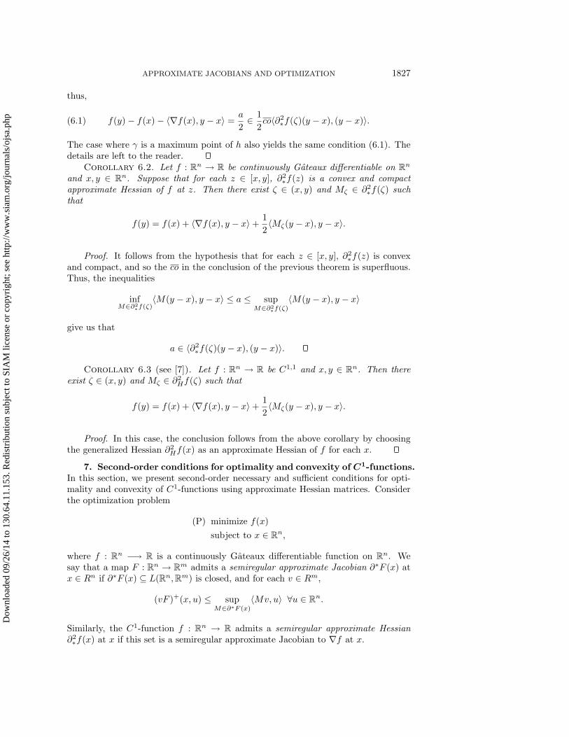
thus,

(6.1) f(y)− f(x)− 〈∇f(x), y − x〉 =a

2∈ 1

2co〈∂2

∗f(ζ)(y − x), (y − x)〉.

The case where γ is a maximum point of h also yields the same condition (6.1). Thedetails are left to the reader.

Corollary 6.2. Let f : Rn → R be continuously Gateaux differentiable on Rnand x, y ∈ Rn. Suppose that for each z ∈ [x, y], ∂2

∗f(z) is a convex and compactapproximate Hessian of f at z. Then there exist ζ ∈ (x, y) and Mζ ∈ ∂2

∗f(ζ) suchthat

f(y) = f(x) + 〈∇f(x), y − x〉+1

2〈Mζ(y − x), y − x〉.

Proof. It follows from the hypothesis that for each z ∈ [x, y], ∂2∗f(z) is convex

and compact, and so the co in the conclusion of the previous theorem is superfluous.Thus, the inequalities

infM∈∂2∗f(ζ)

〈M(y − x), y − x〉 ≤ a ≤ supM∈∂2∗f(ζ)

〈M(y − x), y − x〉

give us that

a ∈ 〈∂2∗f(ζ)(y − x), (y − x)〉.

Corollary 6.3 (see [7]). Let f : Rn → R be C1,1 and x, y ∈ Rn. Then thereexist ζ ∈ (x, y) and Mζ ∈ ∂2

Hf(ζ) such that

f(y) = f(x) + 〈∇f(x), y − x〉+1

2〈Mζ(y − x), y − x〉.

Proof. In this case, the conclusion follows from the above corollary by choosingthe generalized Hessian ∂2

Hf(x) as an approximate Hessian of f for each x.

7. Second-order conditions for optimality and convexity of C1-functions.In this section, we present second-order necessary and sufficient conditions for opti-mality and convexity of C1-functions using approximate Hessian matrices. Considerthe optimization problem

(P) minimize f(x)

subject to x ∈ Rn,

where f : Rn −→ R is a continuously Gateaux differentiable function on Rn. Wesay that a map F : Rn → Rm admits a semiregular approximate Jacobian ∂∗F (x) atx ∈ Rn if ∂∗F (x) ⊆ L(Rn,Rm) is closed, and for each v ∈ Rm,

(vF )+(x, u) ≤ supM∈∂∗F (x)

〈Mv, u〉 ∀u ∈ Rn.

Similarly, the C1-function f : Rn → R admits a semiregular approximate Hessian∂2∗f(x) at x if this set is a semiregular approximate Jacobian to ∇f at x.

Dow

nloa

ded

09/2

6/14

to 1

30.6

4.11

.153

. Red

istr

ibut

ion

subj

ect t

o SI

AM

lice

nse

or c

opyr

ight

; see

http

://w

ww

.sia

m.o

rg/jo

urna

ls/o

jsa.

php


Of course, every semiregular approximate Hessian to f at x is an approximateHessian at x. For a C1,1 function f : Rn → R, the generalized Hessian, ∂2

Hf(x), of fat x is a bounded semiregular approximate Hessian of f at x since

(v∇f)+(x, u) ≤ f(x;u, v) = maxM∈∂2

Hf(x)〈Mu, v〉 = max

M∈∂2Hf(x)〈Mv, u〉.

Theorem 7.1. For the problem (P), let x ∈ Rn. Assume that ∂2∗f(x) is a

semiregular approximate Hessian of f at x.(i) If x is a local minimum of (P), then ∇f(x) = 0, and for each u ∈ IRn,

supM∈∂2∗f(x)

〈Mu, u〉 ≥ 0.

(ii) If x is a local maximum of (P), then ∇f(x) = 0, and for each u ∈ Rn,

infM∈∂2∗f(x)

〈Mu, u〉 ≤ 0.

Proof. Let u ∈ Rn. Since x is a local minimum of (P), there exists δ > 0 suchthat for each s ∈ [0, δ],

f(x+ su) ≥ f(x).

Then, by the mean value theorem, for each s ∈ (0, δ], there exists 0 < t < s such that

〈∇f(x+ tu), u〉 ≥ 0.

So, there exists a positive sequence tn ↓ 0 such that 〈∇f(x+ tnu), u〉 ≥ 0. Now, as∇f(x) = 0, it follows that

(u∇f)+(x;u) = lim sups↓0

〈∇f(x+ su), u〉 − 〈∇f(x), u〉s

≥ 0.

Since ∂2∗f(x) is a semiregular approximate Hessian of f at x, we have

(u∇f)+(x;u) ≤ supM∈∂2∗f(x)

〈Mu, u〉,

and hence,

supM∈∂2∗f(x)

〈Mu, u〉 ≥ 0.

On the other hand, if f attains a local maximum at x, then it follows by thesimilar arguments as above that for each u ∈ Rn,

infM∈∂2∗f(x)

〈Mu, u〉 ≤ 0.

Note in this case that it is convenient to use the inequality

(u∇f)−(x, u) ≥ infM∈∂2∗f(x)

〈Mu, u〉.

Dow

nloa

ded

09/2

6/14

to 1

30.6

4.11

.153

. Red

istr

ibut

ion

subj

ect t

o SI

AM

lice

nse

or c

opyr

ight

; see

http

://w

ww

.sia

m.o

rg/jo

urna

ls/o

jsa.

php


Let us look at a numerical example to illustrate the significance of the optimalityconditions obtained in the previous theorem.

Example 7.2. Define f : R2 → R by

f(x, y) =2

3|x| 32 +

1

2y2.

Then f is C1 but is not C1,1 since the gradient

∇f(x, y) =(√|x| sgn(x), y

)is not locally Lipschitz at (0, 0). Evidently, (0, 0) is a minimum point of f , ∇f(0, 0) =(0, 0), and

∂2∗f(0) =

(α 00 1

): α ≥ 0

is a semiregular approximate Hessian of f at (0, 0). And for each u = (u1, u2) ∈ R2,

supM∈∂2∗f(0)

〈Mu, u〉 = supαu21 + u2

2 : α ≥ 0 ≥ 0.

Hence, the statement (i) of Theorem 7.1 is verified. However, the generalized Hessians[7] do not apply to this function.

Corollary 7.3. For the problem (P), let x ∈ Rn. Suppose that ∂2∗f(x) is a

bounded semiregular approximate Hessian of f at x.(i) If x is a local minimum of (P), then ∇f(x) = 0, and for each u ∈ Rn there

exists a matrix M ∈ ∂2∗f(x) such that 〈Mu, u〉 ≥ 0.

(ii) If x is a local maximum of (P), then ∇f(x) = 0, and for each u ∈ Rn thereexists a matrix M ∈ ∂2

∗f(x) such that 〈Mu, u〉 ≤ 0.Proof. Since ∂2

∗f(x) is closed and bounded, it follows from Theorem 7.1 that∇f(x) = 0, and for each u ∈ IRn,

maxM∈∂2∗f(x)

〈Mu, u〉 ≥ 0,

and so the first conclusion holds. The second conclusion similarly follows from Theo-rem 7.1.

We now see how optimality conditions for the problem (P ) where f is C1,1 followsfrom Corollary 7.3 (cf. [7]).

Corollary 7.4. For the problem (P), assume that the function f is C1,1 andx ∈ Rn.

(i) If x is a local minimum of (P), then ∇f(x) = 0, and for each u ∈ Rn thereexists a matrix M ∈ ∂2

Hf(x) such that 〈Mu, u〉 ≥ 0.(ii) If x is a local maximum of (P), then ∇f(x) = 0, and for each u ∈ Rn there

exists a matrix M ∈ ∂2Hf(x) such that 〈Mu, u〉 ≤ 0.

Proof. The conclusion follows from Corollary 7.3 by choosing ∂2Hf(x) as the

semiregular bounded approximate Hessian ∂2∗f(x) of f at x.

Clearly, the conditions of Theorem 7.1 are not sufficient for a local minimum,even for a C2-function f . The generalized Taylor’s expansion is now applied to obtaina version of second-order sufficient condition for a local minimum. For related results,see [34, 16].

Dow

nloa

ded

09/2

6/14

to 1

30.6

4.11

.153

. Red

istr

ibut

ion

subj

ect t

o SI

AM

lice

nse

or c

opyr

ight

; see

http

://w

ww

.sia

m.o

rg/jo

urna

ls/o

jsa.

php


Theorem 7.5. For the problem (P), let x ∈ Rn. Assume that for each x in aneighborhood of x, ∂2

∗f(x) is a bounded approximate Hessian of f at x. If ∇f(x) = 0and for 0 < α < 1, each u ∈ Rn satisfies u 6= 0; then the following holds:

(7.1) (∀M ∈ co(∂2∗f(x+ αu))), 〈Mu, u〉 ≥ 0.

Then x is a local minimum of (P).Proof. Suppose that x is not a local minimum of (P ). Then there exists a sequence

xn such that xn 6= x, xn −→ x as n −→ +∞, and f(xn) < f(x) for each n. Letxn = x + un, where un 6= 0. From the generalized Taylor expansion, Theorem 6.1,there exists 0 < αn < 1 such that

f(xn) ∈ f(x) + 〈∇f(x), xn − x〉+1

2co〈∂2

∗f(x+ αnun)(un), un〉.

Thus, there exists Mn ∈ co(∂2∗f(x + αnun)) such that f(xn) = f(x) + 〈Mnun, un〉,

and so 〈Mnun, un〉 < 0. This contradicts (7.1). Hence, x is a local minimum of(P).

The following theorem gives us second-order sufficient optimality conditions for astrict local minimum.

Theorem 7.6. For the problem (P), let x ∈ Rn. Assume that, for each x in aneighborhood of x, ∂2

∗f(x) is a bounded approximate Hessian of f at x. If ∇f(x) = 0and for 0 < α < 1, each u ∈ Rn satisfies u 6= 0, then the following holds:

(7.2) (∀M ∈ co(∂2∗f(x+ αu))), 〈Mu, u〉 > 0.

Then x is a strict local minimum of (P).Proof. The method of proof is similar to the one given above for Theorem 7.5

and so it is omitted.We now see how the mean value theorem of section 3 and approximate Hessians

can be used to characterize convexity of C1- functions.Theorem 7.7. Let f : Rn → R be a continuously Gateaux differentiable function.

Assume that ∂2∗f(x) is an approximate Hessian of f for each point x ∈ Rn. If the

matrices M ∈ ∂2∗f(x) are positive semidefinite for each x ∈ Rn, then f is convex.

Proof. Let x, u ∈ Rn. Then, by the mean value theorem,

∇f(x+ u)−∇f(x) ∈ co(∂2∗f([x, x+ u])u),

and so,

〈∇f(x+ u)−∇f(x), u〉 ∈ 〈co(∂2∗f([x, x+ u])u), u〉.

Thus, there exist z ∈ [x, x+ u] and M ∈ co(∂2∗f(z)) such that

〈∇f(x+ u)−∇f(x), u〉 = 〈Mu, u〉.It follows by the assumption that

〈∇f(x+ u)−∇f(x), u〉 ≥ 0.

Since x, u ∈ Rn are arbitrary, we get that ∇f is monotone in the sense that for eachx, u ∈ Rn,

〈∇f(x+ u)−∇f(x), u〉 ≥ 0.

Dow

nloa

ded

09/2

6/14

to 1

30.6

4.11

.153

. Red

istr

ibut

ion

subj

ect t

o SI

AM

lice

nse

or c

opyr

ight

; see

http

://w

ww

.sia

m.o

rg/jo

urna

ls/o

jsa.

php


The conclusion now follows from the standard result of convex analysis that f isconvex if and only if ∇f is monotone.

Corollary 7.8. Let f : Rn → R be C1,1. Then f is convex if and only if foreach x ∈ Rn, the matrices M ∈ ∂2

Hf(x) are positive semidefinite.Proof. Since f is C1,1 for each x ∈ Rn, ∂2

Hf(x) is an approximate Hessian of f atx. Hence, it follows from Theorem 7.7 that f is convex.

Conversely, assume that f is convex. Let ∆ be a set of points in Rn on which fis twice differentiable. Then, each matrix M of

limn→∞∇

2f(xn) : xn ⊂ ∆, xn → x

is positive semidefinite as it is a limit of a sequence of positive semidefinite matrices.Hence, each matrix M of

∂2Hf(x) = co lim

n→∞∇2f(xn) : xn ⊂ ∆, xn → x

is also positive semidefinite.

Acknowledgments. The authors are grateful to the referees for their detailedcomments and valuable suggestions which have contributed to the final preparation ofthe paper. The first author is grateful to Professor Jonathan Borwein for his helpfulcomments on the earlier version of the paper and for certain useful references. Thesecond author wishes to thank the first author for his kind invitation and hospitality.

REFERENCES

[1] F. H. Clarke, Necessary Conditions for Pproblems in Optimal Control and Calculus of Vari-ations, Ph.D. Thesis, University of Washington, Seattle, 1973.

[2] F. H. Clarke, Optimization and nonsmooth analysis, Wiley-Interscience, New York, 1983.[3] R. Cominetti and R. Correa, A generalized second-order derivative in nonsmooth optimiza-

tion, SIAM J. Control and Optim., 28 (1990), pp. 789–809.[4] V. F. Demyanov and V. Jeyakumar, Hunting for a smaller convex subdifferential, J. Global

Optim., 10 (1997), pp. 305–326.[5] V. F. Demyanov and A. M. Rubinov, Constructive Nonsmooth Analysis, Verlag Peter Lang,

Frankfurt am Main, 1995.[6] J. -B. Hiriart-Urruty, Mean value theorems for vector valued mappings in nonsmooth opti-

mization, Numer. Funct. Anal. Optim., 2 (1980), pp. 1–30.[7] J. B. Hiriart-Urruty, J. J. Strodiot, and V. Hien Nguyen, Generalized Hessian matrix

and second-order optimality conditions for problems with C1,1 data, Appl. Math. Optim.,11 (1984), pp. 43–56.

[8] A. D. Ioffe, Nonsmooth Analysis: differential calculus of nondifferential mappings, Trans.Amer. Math. Soc., 266 (1981), pp. 1–56.

[9] A. D. Ioffe, Approximate subdifferentials and applications I: The finite dimensional theory,Trans. Amer. Math. Soc., 281 (1984), pp. 389–416.

[10] A. D. Ioffe and J. -P. Penot, Limiting subhessians and limiting subjects and their calculus,Trans. Amer. Math. Soc., 349 (1997), pp. 789–808.

[11] V. Jeyakumar, On optimality conditions in nonsmooth inequality constrained minimization,Numer. Funct. Anal. Optim., 9 (1987), pp. 535–546.

[12] V. Jeyakumar, Composite nonsmooth programming with Gateaux differentiability, SIAM J.Optim., 1 (1991), pp. 30–41.

[13] V. Jeyakumar and D. T. Luc, Nonsmooth Calculus, Minimality and Monotonicity of Con-vexificators, Applied Mathematics Research Report AMR96/29, University of New SouthWales, Australia, 1996, submitted.

[14] V. Jeyakumar and X. Q. Yang, Convex composite multi-objective nonsmooth programming,Math. Progr., 59 (1993), pp. 325–343.

[15] V. Jeyakumar and X. Q. Yang, Convex composite minimization with C1,1 functions, J.Optim. Theory Appl., 86 (1995), pp. 631–648.

Dow

nloa

ded

09/2

6/14

to 1

30.6

4.11

.153

. Red

istr

ibut

ion

subj

ect t

o SI

AM

lice

nse

or c

opyr

ight

; see

http

://w

ww

.sia

m.o

rg/jo

urna

ls/o

jsa.

php


[16] V. Jeyakumar and X. Q. Yang, Approximate Generalized Hessians and Taylor’s Expansionsfor Continuously Gateaux Differentiable Functions, Applied Mathematics Research ReportAMR96/20, University of New South Wales, Australia, Nonlinear Anal., 1998, to appear.

[17] D. T. Luc, Taylor’s formula for Ck,1 functions, SIAM J. Optim., 5 (1995), pp. 659–669.[18] D. T. Luc and S. Schaible, On generalized monotone nonsmooth maps, J. Convex Anal., 3

(1996), pp. 195–205.[19] D. T. Luc and S. Swaminathan, A characterization of convex functions, Nonlinear Anal., 20

(1993), pp. 697–701.[20] P. Michel and J.-P. Penot, A generalized derivative for calm and stable functions, Differen-

tial Integral Equations, 5 (1992), pp. 433–454.[21] B. S. Mordukhovich, Metric approximations and necessary optimality conditions for general

classes of nonsmooth extremal problems, Soviet. Math. Dokl., 22 (1980), pp. 526–530.[22] B. S. Mordukhovich, Generalized differential calculus for nonsmooth and set-valued map-

pings, J. Math. Anal. Appl., 183 (1994), pp. 250–288.[23] B. S. Mordukhovich and Y. Shao, On nonconvex subdifferential calculus in Banach spaces,

J. Convex Anal., 2 (1995), pp. 211–228.[24] B. S. Mordukhovich and Y. Shao, Nonsmooth sequential analysis in Asplund spaces, Trans.

Amer. Math. Soc., 348 (1996), pp. 1235–1280.[25] Z. Pales and V. Zeidan, Generalized Hessian for C1,1 functions in infinite dimensional

normed spaces, Math. Programming, 74 (1996), pp. 59–78.[26] J. S. Pang and L. Qi, Nonsmooth equations: Motivation and algorithms, SIAM J. Optim., 3

(1993), pp. 443–465.[27] R. T. Rockafellar, Generalized directional derivatives and subgradient of nonconvex func-

tions, Canad. J. Math., 32 (1980), pp. 257–280.[28] R. T. Rockafellar, Second-order optimality conditions in nonlinear programming obtained

by way of epi-derivatives, Math. Oper. Res., 14 (1989), pp. 462–484.[29] R. T. Rockafellar and J. B. Wets, Variational Analysis, Springer-Verlag, Berlin, New

York, 1998, to appear.[30] M. Studniarski and V. Jeyakumar, A generalized mean-value theorem and optimality con-

ditions in composite nonsmooth minimization, Nonlinear Anal., 24 (1995), pp. 883–894.[31] L. Thibault, On generalized differentials and subdifferentials of Lipschitz vector valued func-

tions, Nonlinear Anal., 6 (1982), pp. 1037–1053.[32] J. Warga, Derivative containers, inverse functions and controllability, in Calculus of Varia-

tions and Control Theory, D.L. Russell, ed., Academic Press, New York, 1976.[33] J. Warga, Fat homeomorphisms and unbounded derivative containers, J. Math. Anal. Appl.,

81 (1981), pp. 545–560.[34] X. Q. Yang, Generalized Second-Order Directional Derivatives and Optimality Conditions,

Ph.D. thesis, University of New South Wales, Australia, 1994.[35] X. Q. Yang and V. Jeyakumar, Generalized second-order directional derivatives and opti-

mization with C1,1 functions, Optimization, 26 (1992), pp. 165–185.

Dow

nloa

ded

09/2

6/14

to 1

30.6

4.11

.153

. Red

istr

ibut

ion

subj

ect t

o SI

AM

lice

nse

or c

opyr

ight

; see

http

://w

ww

.sia

m.o

rg/jo

urna

ls/o

jsa.

php

Documents

Approximate Jacobian Matrices for Nonsmooth Continuous Maps and C 1 -Optimization