Embed Size (px)
Citation preview
Normalizing Flow Models
Stefano Ermon, Aditya Grover
Stanford University
Lecture 7
Stefano Ermon, Aditya Grover (AI Lab) Deep Generative Models Lecture 7 1 / 21
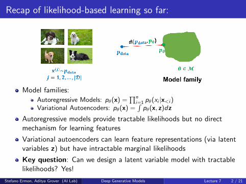
Recap of likelihood-based learning so far:
Model families:
Autoregressive Models: pθ(x) =∏n
i=1 pθ(xi |x<i )Variational Autoencoders: pθ(x) =
∫pθ(x, z)dz
Autoregressive models provide tractable likelihoods but no directmechanism for learning features
Variational autoencoders can learn feature representations (via latentvariables z) but have intractable marginal likelihoods
Key question: Can we design a latent variable model with tractablelikelihoods? Yes!
Stefano Ermon, Aditya Grover (AI Lab) Deep Generative Models Lecture 7 2 / 21
Simple Prior to Complex Data Distributions
Desirable properties of any model distribution:
Analytic densityEasy-to-sample
Many simple distributions satisfy the above properties e.g., Gaussian,uniform distributions
Unfortunately, data distributions could be much more complex(multi-modal)
Key idea: Map simple distributions (easy to sample and evaluatedensities) to complex distributions (learned via data) using change ofvariables.
Stefano Ermon, Aditya Grover (AI Lab) Deep Generative Models Lecture 7 3 / 21
Change of Variables formula
Let Z be a uniform random variable U [0, 2] with density pZ . What ispZ (1)? 1
2
Let X = 4Z , and let pX be its density. What is pX (4)?
pX (4) = p(X = 4) = p(4Z = 4) = p(Z = 1) = pZ (1) = 1/2 No
Clearly, X is uniform in [0, 8], so pX (4) = 1/8
Stefano Ermon, Aditya Grover (AI Lab) Deep Generative Models Lecture 7 4 / 21
Change of Variables formula
Change of variables (1D case): If X = f (Z ) and f (·) is monotonewith inverse Z = f −1(X ) = h(X ), then:
pX (x) = pZ (h(x))|h′(x)|
Previous example: If X = 4Z and Z ∼ U [0, 2], what is pX (4)?
Note that h(X ) = X/4
pX (4) = pZ (1)h′(4) = 1/2× 1/4 = 1/8
Stefano Ermon, Aditya Grover (AI Lab) Deep Generative Models Lecture 7 5 / 21
Geometry: Determinants and volumes
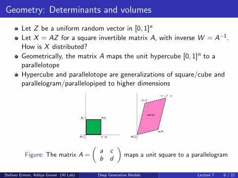
Let Z be a uniform random vector in [0, 1]n
Let X = AZ for a square invertible matrix A, with inverse W = A−1.How is X distributed?
Geometrically, the matrix A maps the unit hypercube [0, 1]n to aparallelotope
Hypercube and parallelotope are generalizations of square/cube andparallelogram/parallelopiped to higher dimensions
Figure: The matrix A =
(a cb d
)maps a unit square to a parallelogram
Stefano Ermon, Aditya Grover (AI Lab) Deep Generative Models Lecture 7 6 / 21
Geometry: Determinants and volumes
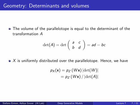
The volume of the parallelotope is equal to the determinant of thetransformation A
det(A) = det
(a cb d
)= ad − bc
X is uniformly distributed over the parallelotope. Hence, we have
pX (x) = pZ (W x) |det(W )|= pZ (W x) / |det(A)|
Stefano Ermon, Aditya Grover (AI Lab) Deep Generative Models Lecture 7 7 / 21
Generalized change of variables
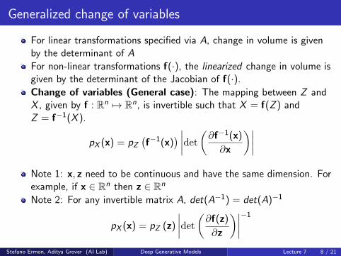
For linear transformations specified via A, change in volume is givenby the determinant of A
For non-linear transformations f(·), the linearized change in volume isgiven by the determinant of the Jacobian of f(·).
Change of variables (General case): The mapping between Z andX , given by f : Rn 7→ Rn, is invertible such that X = f(Z ) andZ = f−1(X ).
pX (x) = pZ(f−1(x)
) ∣∣∣∣det(∂f−1(x)
∂x
)∣∣∣∣Note 1: x, z need to be continuous and have the same dimension. Forexample, if x ∈ Rn then z ∈ Rn
Note 2: For any invertible matrix A, det(A−1) = det(A)−1
pX (x) = pZ (z)
∣∣∣∣det(∂f(z)
∂z
)∣∣∣∣−1Stefano Ermon, Aditya Grover (AI Lab) Deep Generative Models Lecture 7 8 / 21
Two Dimensional Example
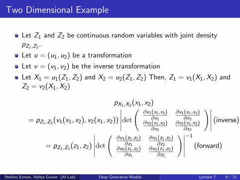
Let Z1 and Z2 be continuous random variables with joint densitypZ1,Z2 .
Let u = (u1, u2) be a transformation
Let v = (v1, v2) be the inverse transformation
Let X1 = u1(Z1,Z2) and X2 = u2(Z1,Z2) Then, Z1 = v1(X1,X2) andZ2 = v2(X1,X2)
pX1,X2(x1, x2)
= pZ1,Z2(v1(x1, x2), v2(x1, x2))
∣∣∣∣∣det(
∂v1(x1,x2)∂x1
∂v1(x1,x2)∂x2
∂v2(x1,x2)∂x1
∂v2(x1,x2)∂x2
)∣∣∣∣∣ (inverse)
= pZ1,Z2(z1, z2)
∣∣∣∣∣det(
∂u1(z1,z2)∂z1
∂u1(z1,z2)∂z2
∂u2(z1,z2)∂z1
∂u2(z1,z2)∂z2
)∣∣∣∣∣−1
(forward)
Stefano Ermon, Aditya Grover (AI Lab) Deep Generative Models Lecture 7 9 / 21
Normalizing flow models
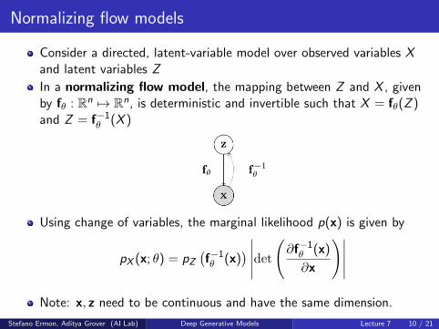
Consider a directed, latent-variable model over observed variables Xand latent variables Z
In a normalizing flow model, the mapping between Z and X , givenby fθ : Rn 7→ Rn, is deterministic and invertible such that X = fθ(Z )and Z = f−1θ (X )
Using change of variables, the marginal likelihood p(x) is given by
pX (x; θ) = pZ(f−1θ (x)
) ∣∣∣∣∣det(∂f−1θ (x)
∂x
)∣∣∣∣∣Note: x, z need to be continuous and have the same dimension.
Stefano Ermon, Aditya Grover (AI Lab) Deep Generative Models Lecture 7 10 / 21
A Flow of Transformations
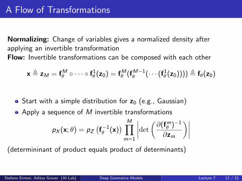
Normalizing: Change of variables gives a normalized density afterapplying an invertible transformationFlow: Invertible transformations can be composed with each other
x , zM = fMθ ◦ · · · ◦ f1θ (z0) = fMθ (fM−1θ (· · · (f1θ (z0)))) , fθ(z0)
Start with a simple distribution for z0 (e.g., Gaussian)
Apply a sequence of M invertible transformations
pX (x; θ) = pZ(f−1θ (x)
) M∏m=1
∣∣∣∣det(∂(fmθ )−1
∂zm
)∣∣∣∣(determininant of product equals product of determinants)
Stefano Ermon, Aditya Grover (AI Lab) Deep Generative Models Lecture 7 11 / 21
Planar flows
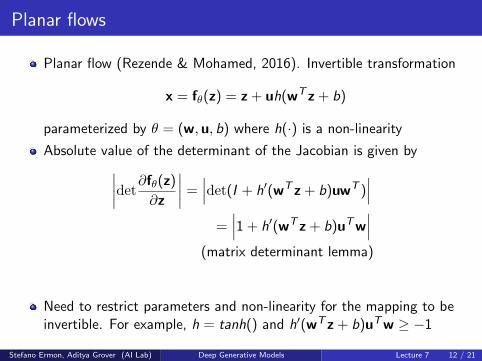
Planar flow (Rezende & Mohamed, 2016). Invertible transformation
x = fθ(z) = z + uh(wTz + b)
parameterized by θ = (w,u, b) where h(·) is a non-linearity
Absolute value of the determinant of the Jacobian is given by∣∣∣∣det∂fθ(z)
∂z
∣∣∣∣ =∣∣∣det(I + h′(wTz + b)uwT )
∣∣∣=∣∣∣1 + h′(wTz + b)uTw
∣∣∣(matrix determinant lemma)
Need to restrict parameters and non-linearity for the mapping to beinvertible. For example, h = tanh() and h′(wTz + b)uTw ≥ −1
Stefano Ermon, Aditya Grover (AI Lab) Deep Generative Models Lecture 7 12 / 21
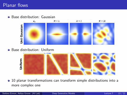
Planar flows
Base distribution: Gaussian
Base distribution: Uniform
10 planar transformations can transform simple distributions into amore complex one
Stefano Ermon, Aditya Grover (AI Lab) Deep Generative Models Lecture 7 13 / 21
Learning and Inference
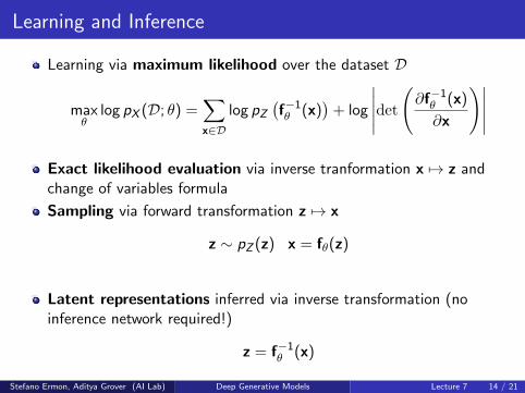
Learning via maximum likelihood over the dataset D
maxθ
log pX (D; θ) =∑x∈D
log pZ(f−1θ (x)
)+ log
∣∣∣∣∣det(∂f−1θ (x)
∂x
)∣∣∣∣∣Exact likelihood evaluation via inverse tranformation x 7→ z andchange of variables formula
Sampling via forward transformation z 7→ x
z ∼ pZ (z) x = fθ(z)
Latent representations inferred via inverse transformation (noinference network required!)
z = f−1θ (x)
Stefano Ermon, Aditya Grover (AI Lab) Deep Generative Models Lecture 7 14 / 21
Desiderata for flow models
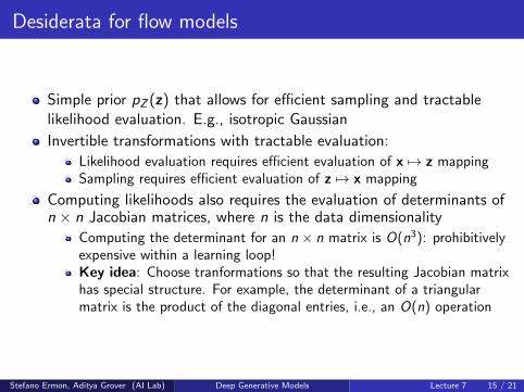
Simple prior pZ (z) that allows for efficient sampling and tractablelikelihood evaluation. E.g., isotropic Gaussian
Invertible transformations with tractable evaluation:
Likelihood evaluation requires efficient evaluation of x 7→ z mappingSampling requires efficient evaluation of z 7→ x mapping
Computing likelihoods also requires the evaluation of determinants ofn × n Jacobian matrices, where n is the data dimensionality
Computing the determinant for an n × n matrix is O(n3): prohibitivelyexpensive within a learning loop!Key idea: Choose tranformations so that the resulting Jacobian matrixhas special structure. For example, the determinant of a triangularmatrix is the product of the diagonal entries, i.e., an O(n) operation
Stefano Ermon, Aditya Grover (AI Lab) Deep Generative Models Lecture 7 15 / 21
Triangular Jacobian
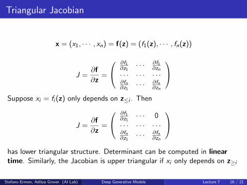
x = (x1, · · · , xn) = f(z) = (f1(z), · · · , fn(z))
J =∂f
∂z=
∂f1∂z1
· · · ∂f1∂zn
· · · · · · · · ·∂fn∂z1
· · · ∂fn∂zn
Suppose xi = fi (z) only depends on z≤i . Then
J =∂f
∂z=
∂f1∂z1
· · · 0
· · · · · · · · ·∂fn∂z1
· · · ∂fn∂zn
has lower triangular structure. Determinant can be computed in lineartime. Similarly, the Jacobian is upper triangular if xi only depends on z≥i
Stefano Ermon, Aditya Grover (AI Lab) Deep Generative Models Lecture 7 16 / 21
Designing invertible transformations
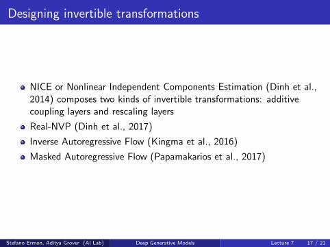
NICE or Nonlinear Independent Components Estimation (Dinh et al.,2014) composes two kinds of invertible transformations: additivecoupling layers and rescaling layers
Real-NVP (Dinh et al., 2017)
Inverse Autoregressive Flow (Kingma et al., 2016)
Masked Autoregressive Flow (Papamakarios et al., 2017)
Stefano Ermon, Aditya Grover (AI Lab) Deep Generative Models Lecture 7 17 / 21
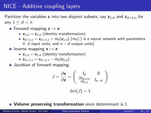
NICE - Additive coupling layers
Partition the variables z into two disjoint subsets, say z1:d and zd+1:n forany 1 ≤ d < n
Forward mapping z 7→ x:x1:d = z1:d (identity transformation)xd+1:n = zd+1:n + mθ(z1:d) (mθ(·) is a neural network with parametersθ, d input units, and n − d output units)
Inverse mapping x 7→ z:z1:d = x1:d (identity transformation)zd+1:n = xd+1:n −mθ(x1:d)
Jacobian of forward mapping:
J =∂x
∂z=
(Id 0
∂xd+1:n
∂z1:dIn−d
)
det(J) = 1
Volume preserving transformation since determinant is 1.
Stefano Ermon, Aditya Grover (AI Lab) Deep Generative Models Lecture 7 18 / 21
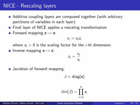
NICE - Rescaling layers
Additive coupling layers are composed together (with arbitrarypartitions of variables in each layer)
Final layer of NICE applies a rescaling transformation
Forward mapping z 7→ x:xi = sizi
where si > 0 is the scaling factor for the i-th dimension.
Inverse mapping x 7→ z:
zi =xisi
Jacobian of forward mapping:
J = diag(s)
det(J) =n∏
i=1
si
Stefano Ermon, Aditya Grover (AI Lab) Deep Generative Models Lecture 7 19 / 21
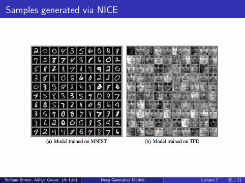
Samples generated via NICE
Stefano Ermon, Aditya Grover (AI Lab) Deep Generative Models Lecture 7 20 / 21
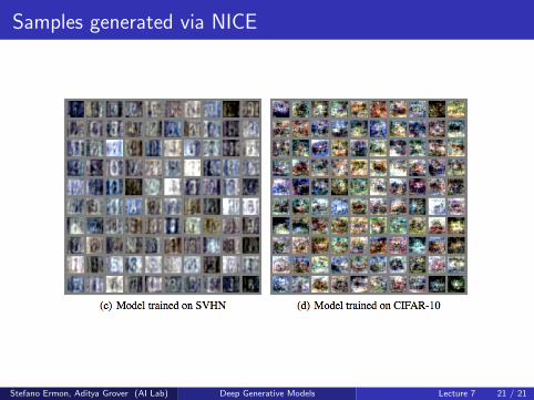
Samples generated via NICE
Stefano Ermon, Aditya Grover (AI Lab) Deep Generative Models Lecture 7 21 / 21