Embed Size (px)
Citation preview
TRANSLATION VALIDATION OF OPTIMIZING TRANSFORMATIONS OF
PROGRAMS USING EQUIVALENCE CHECKING
Kunal Banerjee

TRANSLATION VALIDATION OF OPTIMIZING TRANSFORMATIONS OF
PROGRAMS USING EQUIVALENCE CHECKING
Thesis submitted in partial fulfillmentof the requirements for the award of the degree
of
Doctor of Philosophy
by
Kunal Banerjee
Under the supervision of
Dr. Chittaranjan Mandaland
Dr. Dipankar Sarkar
Department of Computer Science and Engineering
Indian Institute of Technology Kharagpur
July 2015
c© 2015 Kunal Banerjee. All Rights Reserved.

APPROVAL OF THE VIVA-VOCE BOARD
Certified that the thesis entitled “Translation Validation of Optimizing Trans-formations of Programs using Equivalence Checking,” submitted by KunalBanerjee to the Indian Institute of Technology Kharagpur, for the award of thedegree of Doctor of Philosophy has been accepted by the external examinersand that the student has successfully defended the thesis in the viva-voce ex-amination held today.
Prof Sujoy Ghose Prof Pallab Dasgupta(Member of the DSC) (Member of the DSC)
Prof Santanu Chattopadhyay(Member of the DSC)
Prof Chittaranjan Mandal Prof Dipankar Sarkar(Supervisor) (Supervisor)
(External Examiner) (Chairman)
Date:

CERTIFICATE
This is to certify that the thesis entitled “Translation Validation of Opti-mizing Transformations of Programs using Equivalence Checking,”, sub-mitted by Kunal Banerjee to Indian Institute of Technology Kharagpur, is arecord of bona fide research work under our supervision and we consider itworthy of consideration for the award of the degree of Doctor of Philosophyof the Institute.
Chittaranjan MandalProfessorCSE, IIT Kharagpur
Dipankar SarkarProfessorCSE, IIT Kharagpur
Date:


DECLARATION
I certify that
a. The work contained in this thesis is original and has been done by myselfunder the general supervision of my supervisors.
b. The work has not been submitted to any other Institute for any degree ordiploma.
c. I have followed the guidelines provided by the Institute in writing thethesis.
d. I have conformed to the norms and guidelines given in the Ethical Codeof Conduct of the Institute.
e. Whenever I have used materials (data, theoretical analysis, and text)from other sources, I have given due credit to them by citing them inthe text of the thesis and giving their details in the references.
f. Whenever I have quoted written materials from other sources, I have putthem under quotation marks and given due credit to the sources by citingthem and giving required details in the references.
Kunal Banerjee

ACKNOWLEDGMENTS
Upon embarking on the journey for PhD, I realized that it requires patience,devotion, determination and diligence on a level which I had not experiencedbefore. The fact that I am presently at the stage of submitting my thesis is owedto the contributions of many people. The primary sources of my inspirationhave been my supervisors, Dr Chittaranjan Mandal and Dr Dipankar Sarkar.They have always encouraged me to pursue my goals and have extended theirhelp whenever needed. Secondly, I shall like to express my gratitude to myparents who have always supported me. Thirdly, I shall like to thank my elderbrother, the first PhD in our family, who has been the primary motivator forme to follow the doctoral degree.
Next, I thank my colleagues in our research group namely, Chandan Karfa,Gargi Roy, K K Sharma, Partha De, Soumyadip Bandyopadhyay, SoumyajitDey and Sudakshina Dutta, for all the enriching discussions; I consider myselffortunate to have found such colleagues. I also had the opportunity to spendsome delightful time with my friends Antara, Arindam, Aritra, Ayan, Bijit, Joy,Krishnendu, Mainak, Rajorshee, Satya Gautam, Sayan, Subhomoy, Subhrang-shu, Surajit, and many more; I thank them for their pleasant company. I amgrateful to Bappa who has been the key person in sorting out all the office re-lated work. I am also indebted to all the anonymous reviewers of our papers;irrespective of whether the verdict was favourable or not, I always found theircriticism helpful and they have contributed much in shaping my thesis. Lastly,I thank Tata Consultancy Services (TCS) for awarding me TCS PhD Fellow-ship which included contingency grants and travel grants for visiting confer-ences both within India and abroad; this thesis is largely owed to TCS’s gener-ous support.
Kunal Banerjee

ABSTRACT
A compiler translates a source code into a target code, often with an objectiveto reduce the execution time and/or save critical resources. Thus, it relievesthe programmer of the effort to write an efficient code and instead, allowsfocusing only on the functionality and the correctness of the program beingdeveloped. However, an error in the design or in the implementation of thecompiler may result in software bugs in the target code generated by that com-piler. Translation validation is a formal verification approach for compilerswhereby, each individual translation is followed by a validation phase whichverifies that the target code produced correctly implements the source code.This thesis presents some translation validation techniques for verifying codemotion transformations (while underlining the special treatment required oncourse to handle the idiosyncrasies of array-intensive programs), loop trans-formations and arithmetic transformations in the presence of recurrences; itadditionally relates two competing translation validation techniques namely,bisimulation relation based approach and path based approach.
A symbolic value propagation based equivalence checking technique overthe Finite State Machine with Datapath (FSMD) model has been developedto check the validity of code motion transformations; this method is capableof verifying code motions across loops as well which the previously reportedpath based verification techniques could not.
Bisimulation relation based approach and path based approach provide twoalternatives for translation validation; while the former is beneficial for verify-ing advanced code transformations, such as loop shifting, the latter surpassesin being able to handle non-structure preserving transformations and guaran-teeing termination. We have developed methods to derive bisimulation rela-tions from the outputs of the path based equivalence checkers to relate thesecompeting translation validation techniques.
The FSMD model has been extended to handle code motion transforma-tions of array-intensive programs with the array references represented usingMcCarthy’s read and write functions. This improvement has necessitated ad-dition of some grammar rules in the normal form used for representing arith-metic expressions that occur in the datapath; the symbolic value propagationbased equivalence checking scheme is also adapted to work with the extendedmodel.
Compiler optimization of array-intensive programs involves extensive ap-plication of loop transformations and arithmetic transformations. A majorobstacle for translation validation of such programs is posed by recurrences,which essentially lead to cycles in the data-dependence graphs of the programsmaking dependence analyses and simplifications of the data transformationsdifficult. A validation scheme is developed for such programs by isolatingthe cycles in the data-dependence graphs from the acyclic portions and treat-ing them separately. Thus, this work provides a unified equivalence checkingframework to handle loop and arithmetic transformations along with recur-

xiv
rences.
Keywords: Translation Validation, Equivalence Checking, BisimulationRelation, Code Motion Transformation, Loop Transformation, Arithmetic Trans-formation, Recurrence, Finite State Machine with Datapath (FSMD), ArrayData Dependence Graph (ADDG)
Contents
Abstract xiii
Table of Contents xv
List of Symbols xix
List of Figures xxi
List of Tables xxiii
1 Introduction 11.1 Literature survey and motivations . . . . . . . . . . . . . . . . . . . . 2
1.1.1 Code motion transformations . . . . . . . . . . . . . . . . . . 31.1.2 Alternative approaches to verification of code motion trans-
formations: bisimulation vs path based . . . . . . . . . . . . 41.1.3 Loop transformations and arithmetic transformations . . . . . 51.1.4 Objectives of the work . . . . . . . . . . . . . . . . . . . . . 7
1.2 Contributions of the thesis . . . . . . . . . . . . . . . . . . . . . . . 81.2.1 Translation validation of code motion transformations . . . . 81.2.2 Deriving bisimulation relations from path based equivalence
checkers . . . . . . . . . . . . . . . . . . . . . . . . . . . . . 91.2.3 Translation validation of code motion transformations in array-
intensive programs . . . . . . . . . . . . . . . . . . . . . . . 91.2.4 Translation validation of loop and arithmetic transformations
in the presence of recurrences . . . . . . . . . . . . . . . . . 111.3 Organization of the thesis . . . . . . . . . . . . . . . . . . . . . . . . 11
2 Literature Survey 132.1 Introduction . . . . . . . . . . . . . . . . . . . . . . . . . . . . . . . 132.2 Code motion transformations . . . . . . . . . . . . . . . . . . . . . . 13
2.2.1 Applications of code motion transformations . . . . . . . . . 132.2.2 Verification of code motion transformations . . . . . . . . . . 16
2.3 Bisimulation vs path based . . . . . . . . . . . . . . . . . . . . . . . 182.3.1 Bisimulation based verification . . . . . . . . . . . . . . . . . 182.3.2 Path based equivalence checking . . . . . . . . . . . . . . . . 20
xv
xvi CONTENTS
2.4 Loop transformations and arithmetic transformations . . . . . . . . . 212.4.1 Applications of loop transformations . . . . . . . . . . . . . . 212.4.2 Applications of arithmetic transformations . . . . . . . . . . 232.4.3 Verification of loop and arithmetic transformations . . . . . . 24
2.5 Conclusion . . . . . . . . . . . . . . . . . . . . . . . . . . . . . . . 27
3 Translation Validation of Code Motion Transformations 293.1 Introduction . . . . . . . . . . . . . . . . . . . . . . . . . . . . . . . 293.2 The FSMD model and related concepts . . . . . . . . . . . . . . . . . 303.3 The method of symbolic value propagation . . . . . . . . . . . . . . 37
3.3.1 Basic concepts . . . . . . . . . . . . . . . . . . . . . . . . . 373.3.2 Need for detecting loop invariance of subexpressions . . . . . 413.3.3 Subsumption of conditions of execution of the paths being
compared . . . . . . . . . . . . . . . . . . . . . . . . . . . . 443.4 Correctness of symbolic value propagation as a method of equivalence
checking . . . . . . . . . . . . . . . . . . . . . . . . . . . . . . . . . 463.5 The overall verification method . . . . . . . . . . . . . . . . . . . . . 49
3.5.1 An illustrative example . . . . . . . . . . . . . . . . . . . . . 523.5.2 An example of dynamic loop scheduling . . . . . . . . . . . . 55
3.6 Correctness and complexity of the equivalence checking procedure . . 583.6.1 Correctness . . . . . . . . . . . . . . . . . . . . . . . . . . . 583.6.2 Complexity . . . . . . . . . . . . . . . . . . . . . . . . . . . 60
3.7 Experimental Results . . . . . . . . . . . . . . . . . . . . . . . . . . 613.8 Conclusion . . . . . . . . . . . . . . . . . . . . . . . . . . . . . . . 64
4 Deriving Bisimulation Relations 674.1 Introduction . . . . . . . . . . . . . . . . . . . . . . . . . . . . . . . 674.2 The FSMD Model . . . . . . . . . . . . . . . . . . . . . . . . . . . . 684.3 From path extension based equivalence checker . . . . . . . . . . . . 704.4 From symbolic value propagation based equivalence checker . . . . . 754.5 Conclusion . . . . . . . . . . . . . . . . . . . . . . . . . . . . . . . 86
5 Code Motion Transformations in Array-Intensive Programs 895.1 Introduction . . . . . . . . . . . . . . . . . . . . . . . . . . . . . . . 895.2 The FSMDA model . . . . . . . . . . . . . . . . . . . . . . . . . . . 905.3 Characteristic tuple of a path . . . . . . . . . . . . . . . . . . . . . . 915.4 Normalization of expressions involving arrays . . . . . . . . . . . . . 925.5 Equivalence checking of FSMDAs . . . . . . . . . . . . . . . . . . . 935.6 Correctness and complexity . . . . . . . . . . . . . . . . . . . . . . . 99
5.6.1 Correctness . . . . . . . . . . . . . . . . . . . . . . . . . . . 995.6.2 Complexity . . . . . . . . . . . . . . . . . . . . . . . . . . . 100
5.7 Experimental Results . . . . . . . . . . . . . . . . . . . . . . . . . . 1015.7.1 Current limitations . . . . . . . . . . . . . . . . . . . . . . . 102
5.8 Conclusion . . . . . . . . . . . . . . . . . . . . . . . . . . . . . . . 103
CONTENTS xvii
6 Loop and Arithmetic Transformations in the Presence of Recurrences 1056.1 Introduction . . . . . . . . . . . . . . . . . . . . . . . . . . . . . . . 1056.2 The class of supported input programs . . . . . . . . . . . . . . . . . 1076.3 The ADDG model and the associated equivalence checking scheme . 108
6.3.1 The ADDG model . . . . . . . . . . . . . . . . . . . . . . . 1086.3.2 Equivalence checking of ADDGs . . . . . . . . . . . . . . . 1136.3.3 An overview of the method . . . . . . . . . . . . . . . . . . . 118
6.4 Extension of the equivalence checking scheme to handle recurrences . 1196.5 Correctness and complexity . . . . . . . . . . . . . . . . . . . . . . . 132
6.5.1 Correctness . . . . . . . . . . . . . . . . . . . . . . . . . . . 1326.5.2 Complexity . . . . . . . . . . . . . . . . . . . . . . . . . . . 135
6.6 Experimental results . . . . . . . . . . . . . . . . . . . . . . . . . . 1366.7 Conclusion . . . . . . . . . . . . . . . . . . . . . . . . . . . . . . . 138
7 Conclusion and Scope for Future Work 1397.1 Summary of contributions . . . . . . . . . . . . . . . . . . . . . . . 1397.2 Scope for future work . . . . . . . . . . . . . . . . . . . . . . . . . . 143
7.2.1 Enhancement of the present work . . . . . . . . . . . . . . . 1437.2.2 Scope of application to other research areas . . . . . . . . . . 145
A Construction of FSMDAs from Behavioural Descriptions 149A.1 How to represent behavioural descriptions as FSMDAs conceptually . 149A.2 How to represent FSMDAs textually . . . . . . . . . . . . . . . . . . 151
Bibliography 155

List of Symbols
M1, M2 Finite State Machines with Datapath (FSMDs) . . . . . . . . . . . . . . . . . . . . . . . 31Qi Set of control states of FSMD Mi . . . . . . . . . . . . . . . . . . . . . . . . . . . . . . . . . . 30qi,0 Reset state of FSMD Mi . . . . . . . . . . . . . . . . . . . . . . . . . . . . . . . . . . . . . . . . . . 30I Set of input variables . . . . . . . . . . . . . . . . . . . . . . . . . . . . . . . . . . . . . . . . . . . . . 30Vi Set of storage variables of FSMD Mi . . . . . . . . . . . . . . . . . . . . . . . . . . . . . . . 30O Set of output variables . . . . . . . . . . . . . . . . . . . . . . . . . . . . . . . . . . . . . . . . . . . . 30τ State transition function of FSMD . . . . . . . . . . . . . . . . . . . . . . . . . . . . . . . . . 30S Set of status expressions . . . . . . . . . . . . . . . . . . . . . . . . . . . . . . . . . . . . . . . . . . 30µ Computation in an FSMD . . . . . . . . . . . . . . . . . . . . . . . . . . . . . . . . . . . . . . . . . 30µ1 ' µ2 Computations µ1 and µ2 are equivalent . . . . . . . . . . . . . . . . . . . . . . . . . . . . . 31M1 vM2 An FSMD M1 is contained in an FSMD M2 . . . . . . . . . . . . . . . . . . . . . . . . . 31q1,i A state of FSMD M1 . . . . . . . . . . . . . . . . . . . . . . . . . . . . . . . . . . . . . . . . . . . . . . 32q2,i A state of FSMD M2 . . . . . . . . . . . . . . . . . . . . . . . . . . . . . . . . . . . . . . . . . . . . . . 32α,β Paths in FSMD . . . . . . . . . . . . . . . . . . . . . . . . . . . . . . . . . . . . . . . . . . . . . . . . . . . 33αs Start state of path al pha . . . . . . . . . . . . . . . . . . . . . . . . . . . . . . . . . . . . . . . . . . . 31α f End (final) state of path α . . . . . . . . . . . . . . . . . . . . . . . . . . . . . . . . . . . . . . . . . 31Rα Condition of execution of the path α . . . . . . . . . . . . . . . . . . . . . . . . . . . . . . . 31rα Data transformation of the path α . . . . . . . . . . . . . . . . . . . . . . . . . . . . . . . . . . 31sα Storage variable transformations of the path α . . . . . . . . . . . . . . . . . . . . . . . 31sα|x Storage variable transformations restricted over the variable x . . . . . . . . . 39θα Output list of the path α . . . . . . . . . . . . . . . . . . . . . . . . . . . . . . . . . . . . . . . . . . . 31P1,P2 Path cover of the FSMDs M1 and M2 . . . . . . . . . . . . . . . . . . . . . . . . . . . . . . . 32α' β Paths α and β are unconditionally equivalent . . . . . . . . . . . . . . . . . . . . . . . . 38α'c β Paths α and β are conditionally equivalent . . . . . . . . . . . . . . . . . . . . . . . . . . 38ϑ Propagated vector . . . . . . . . . . . . . . . . . . . . . . . . . . . . . . . . . . . . . . . . . . . . . . . . 37ϑi, j Propagated vector at state qi, j . . . . . . . . . . . . . . . . . . . . . . . . . . . . . . . . . . . . . . 37υ Initial propagated vector . . . . . . . . . . . . . . . . . . . . . . . . . . . . . . . . . . . . . . . . . . 37ϖi, j Null path at state qi, j . . . . . . . . . . . . . . . . . . . . . . . . . . . . . . . . . . . . . . . . . . . . . . 44δ Set of corresponding state pairs . . . . . . . . . . . . . . . . . . . . . . . . . . . . . . . . . . . . 49δc Set of conditionally corresponding state pairs . . . . . . . . . . . . . . . . . . . . . . . 75qi, j→ qi,k The edge between the states qi, j and qi,k . . . . . . . . . . . . . . . . . . . . . . . . . . . . 52qi, j qi,k The path between the states qi, j and qi,k . . . . . . . . . . . . . . . . . . . . . . . . . . . . . 33
qi, jc−− qi,k
The path between the states qi, j and qi,k having c as its condition of execu-tion . . . . . . . . . . . . . . . . . . . . . . . . . . . . . . . . . . . . . . . . . . . . . . . . . . . . . . . . . . . . . 33
v Vector of variables . . . . . . . . . . . . . . . . . . . . . . . . . . . . . . . . . . . . . . . . . . . . . . . 68
xix
xx CONTENTS
Dv Domain of variables present in the vector v . . . . . . . . . . . . . . . . . . . . . . . . . 68q(v) Set of values assumed by the variables in the state q . . . . . . . . . . . . . . . . . 68σq Data state at q, an individual element of q(v) . . . . . . . . . . . . . . . . . . . . . . . . 68〈q,σ〉 A configuration in an FSMD . . . . . . . . . . . . . . . . . . . . . . . . . . . . . . . . . . . . . . 68η A execution sequence . . . . . . . . . . . . . . . . . . . . . . . . . . . . . . . . . . . . . . . . . . . . . 68Ni Set of all execution sequences in FSMD Mi . . . . . . . . . . . . . . . . . . . . . . . . . 69η1 ≡ η2 Execution sequences η1 and η2 are equivalent . . . . . . . . . . . . . . . . . . . . . . . 69φi, j A relation over the data states at q1,i in M1 and q2, j in M2 . . . . . . . . . . . . 69〈q1,i,q2, j,φi, j〉 A triple in a verification relation . . . . . . . . . . . . . . . . . . . . . . . . . . . . . . . . . . . 69ξ,ζ Walks in FSMD . . . . . . . . . . . . . . . . . . . . . . . . . . . . . . . . . . . . . . . . . . . . . . . . . . 76Rξ Condition of execution of the walk ξ . . . . . . . . . . . . . . . . . . . . . . . . . . . . . . . 76sξ Storage variable transformations of the walk ξ . . . . . . . . . . . . . . . . . . . . . . 76θξ Output list of the walk ξ . . . . . . . . . . . . . . . . . . . . . . . . . . . . . . . . . . . . . . . . . . 76ξ' ζ Walks ξ and ζ are equivalent . . . . . . . . . . . . . . . . . . . . . . . . . . . . . . . . . . . . . . 76qi, j ; qi,k The walk between the states qi, j and qi,k . . . . . . . . . . . . . . . . . . . . . . . . . . . . 69rd McCarthy’s read function . . . . . . . . . . . . . . . . . . . . . . . . . . . . . . . . . . . . . . . . . 91wr McCarthy’s write function . . . . . . . . . . . . . . . . . . . . . . . . . . . . . . . . . . . . . . . . 91G1,G2 Array Data Dependence Graphs (ADDGs) . . . . . . . . . . . . . . . . . . . . . . . . . 108IS Iteration domain of the statement S . . . . . . . . . . . . . . . . . . . . . . . . . . . . . . . 110
SM(d)Z Definition mapping . . . . . . . . . . . . . . . . . . . . . . . . . . . . . . . . . . . . . . . . . . . . . . 110
SDd Definition domain . . . . . . . . . . . . . . . . . . . . . . . . . . . . . . . . . . . . . . . . . . . . . . . 110
SM(u)Yn
Operand mapping . . . . . . . . . . . . . . . . . . . . . . . . . . . . . . . . . . . . . . . . . . . . . . . 110SUYn Operand domain . . . . . . . . . . . . . . . . . . . . . . . . . . . . . . . . . . . . . . . . . . . . . . . . 110SMZ,Yn Dependence mapping . . . . . . . . . . . . . . . . . . . . . . . . . . . . . . . . . . . . . . . . . . . . 111 Right composition operator . . . . . . . . . . . . . . . . . . . . . . . . . . . . . . . . . . . . . . 111g,g1,g2 Slices in ADDG . . . . . . . . . . . . . . . . . . . . . . . . . . . . . . . . . . . . . . . . . . . . . . . . 113rg Data transformation of the slice g . . . . . . . . . . . . . . . . . . . . . . . . . . . . . . . . . 114∂g Characteristic formula of the slice g . . . . . . . . . . . . . . . . . . . . . . . . . . . . . . . 114gDA Definition domain of the slice g . . . . . . . . . . . . . . . . . . . . . . . . . . . . . . . . . . . 114gUV Operand domain of the slice g . . . . . . . . . . . . . . . . . . . . . . . . . . . . . . . . . . . . 114g1 ≈ g2 g1 and g2 are matching IO-slices . . . . . . . . . . . . . . . . . . . . . . . . . . . . . . . . . . 115B1,B2 Basis subgraphs in ADDG . . . . . . . . . . . . . . . . . . . . . . . . . . . . . . . . . . . . . . . 124D1,D2 Induction subgraphs in ADDG . . . . . . . . . . . . . . . . . . . . . . . . . . . . . . . . . . . 125E1,E2 Recurrence subgraphs in ADDG . . . . . . . . . . . . . . . . . . . . . . . . . . . . . . . . . . 126
List of Figures
3.1 (a) M1: Source FSMD. (b) M2: Transformed FSMD. . . . . . . . . . 343.2 An example of symbolic value propagation. . . . . . . . . . . . . . . 393.3 An example of propagation of values across loop. . . . . . . . . . . . 413.4 An example to illustrate the cases Rα⇒ Rβ and Rβ⇒ Rα. . . . . . . . 453.5 Call graph of the proposed verification method. . . . . . . . . . . . . 523.6 FSMDs before and after scheduling. . . . . . . . . . . . . . . . . . . 543.7 An example of dynamic loop scheduling (DLS). . . . . . . . . . . . . 56
4.1 An example showing two execution sequences from two FSMDs. . . . 694.2 An example of non-equivalent programs. . . . . . . . . . . . . . . . . 774.3 An example of code motion across multiple loops. . . . . . . . . . . . 81
5.1 Computing characteristic tuple of a path. . . . . . . . . . . . . . . . . 915.2 Propagation of index variables’ values. . . . . . . . . . . . . . . . . . 945.3 An example of equivalence checking of FSMDAs. . . . . . . . . . . . 97
6.1 Two programs before and after loop transformation. . . . . . . . . . . 1066.2 (a) A nested-loop behaviour. (b) Its corresponding ADDG. . . . . . . 1096.3 A generalized nested loop structure . . . . . . . . . . . . . . . . . . . 1096.4 (a) Original behaviour. (b) Transformed behaviour. . . . . . . . . . . 1166.5 (a) ADDG of the original behaviour. (b) ADDG of the transformed
behaviour. . . . . . . . . . . . . . . . . . . . . . . . . . . . . . . . . 1176.6 An example of two programs containing recurrences. . . . . . . . . . 1206.7 ADDGs for the programs given in Figure 6.6. . . . . . . . . . . . . . 1216.8 Modified subADDGs corresponding to subgraphs marked by the dot-
ted lines in Figure 6.7. . . . . . . . . . . . . . . . . . . . . . . . . . 1226.9 Modified ADDGs with new uninterpreted function for the programs
given in Figure 6.6. . . . . . . . . . . . . . . . . . . . . . . . . . . . 1226.10 An example where back edges exist in the absence of recurrence. . . . 1236.11 (a) Original program. (b) Corresponding ADDG. . . . . . . . . . . . 1276.12 (a) Basis subgraph. (b) Induction subgraph corresponding to Figure 6.11.1286.13 (a) Basis slice. (b) Valid induction slice 1. (c) Valid induction slice 2,
corresponding to Figure 6.8(b). . . . . . . . . . . . . . . . . . . . . . 1286.14 Relationship between different domains. . . . . . . . . . . . . . . . . 132
xxi

xxii LIST OF FIGURES
7.1 A pair of equivalent programs with non-equivalent recurrence graphs. 1437.2 A pair of programs with shift-add multiplication. . . . . . . . . . . . 146
A.1 Construction of FSMDA corresponding to a basic block. . . . . . . . 150A.2 Construction of FSMDA corresponding to a control block. . . . . . . 150A.3 . . . . . . . . . . . . . . . . . . . . . . . . . . . . . . . . . . . . . 151
List of Tables
3.1 Verification results based on our set of benchmarks . . . . . . . . . . 613.2 Verification results based on the benchmarks presented in [95] . . . . 623.3 Verification results based on the benchmarks presented in [90] . . . . 63
5.1 Computation of propagated vectors during equivalence checking ofFSMDAs . . . . . . . . . . . . . . . . . . . . . . . . . . . . . . . . 96
5.2 Verification results of code transformations . . . . . . . . . . . . . . 101
6.1 Results on some benchmarks . . . . . . . . . . . . . . . . . . . . . . 137
xxiii

Chapter 1
Introduction
A compiler is a computer program which translates a source code into a target code,
often with an objective to reduce the execution time and/or save critical resources.
Thus, it relieves the programmer of the duty to write an efficient code and instead,
allows one to focus only on the functionality of a program. Hence, designers advocate
representation of an initial meta-model of a system in the form of a high-level program
which is then transformed through a sequence of optimizations applied by compilers
eventually leading to the final implementation. However, an error in the design or
in the implementation of a compiler may result in software bugs in the target code
obtained from that compiler.
Formal verification can be used to provide guarantees of compiler correctness. It
is an attractive alternative to traditional methods of testing and simulation, which tend
to be time consuming and suffer from incompleteness. There are two fundamental ap-
proaches of formal verification of compilers. The first approach proves that the steps
of the compiler are correct by construction. In this setting, to prove that an optimiza-
tion is correct, one must prove that for any input program the optimization produces
a semantically equivalent program. The primary advantage of correct by construction
techniques is that optimizations are known to be correct when the compiler is built,
before the optimized programs are run even once. Most of the techniques that provide
guarantees of correctness by construction require user interaction [105]. Moreover,
proofs of correctness by construction are harder to achieve because they must show
that any application of the optimization is correct. A correct by construction com-
1
2 Chapter 1 Introduction
piler for the C language is targeted by the CompCert compiler [112]. Since it is very
hard to formally verify all passes of a more general C compiler such as GCC [4], the
optimization passes implemented in CompCert are limited in number. Moreover, un-
decidability of the general problem of program verification restricts the scope of the
input language supported by the verified compiler; for example, the input language
supported by CompCert is Clight [29], a subset of the C language. Therefore, such
correct by construction compilers are still more of an academic interest and are yet
to transcend into industrial practices. It is important to note that even if one cannot
prove a compiler to be correct by construction, one can at least show that, for each
translation that a compiler performs, the output produced has the same behaviour as
the original behaviour. The second category of formal verification approach, called
translation validation, was proposed by Pnueli et al. in [130]; the method consists
in proving correctness each time a sequence of optimization steps is invoked. Here,
each time the compiler runs an optimization, an automated tool tries to prove that the
original program and the corresponding optimized program are equivalent. Although
this approach does not guarantee the correctness of the compilation process, it at least
ensures that any errors in specific instances of translation by the optimizer may be
detected, thereby preventing such errors from propagating any further in the synthesis
process. Another advantage of the translation validation approach is its scope of vali-
dating human expert guided transformations. The present work is aimed at developing
translation validation methodologies for several behavioural transformations. Specif-
ically, we focus on proving functional equivalence between the source behaviour and
the transformed behaviour. It is to be noted that preservation of non-functional prop-
erties, such as timing performance [156], has not been addressed in the current work.
The chapter is organized as follows. Section 1.1 presents a survey of the related
literature and brings out the motivation of the work presented in the thesis. Section 1.2
presents an overview of the thesis work and summarizes the contributions made. Fi-
nally, the outline of the thesis organization is given in Section 1.3.
1.1 Literature survey and motivations
As already discussed, a sequence of transformations may be applied to the source be-
haviour towards obtaining optimal performance in terms of execution time, energy,
1.1 Literature survey and motivations 3
etc., in course of generating the final implementation. In this section, we briefly de-
scribe several such behavioural transformations that are commonly applied by the
compilers and the different verification approaches adopted for their validation.
1.1.1 Code motion transformations
Code motion based transformations, whereby operations are moved across basic block
boundaries, are used widely in the high-level synthesis tools to improve synthesis re-
sults [48, 65, 107]. The objectives of code motions are (i) reduction of number of
computations performed at run-time and (ii) minimization of lifetimes of the tempo-
rary variables to avoid unnecessary register usage. Based on the above objectives,
code motions can be classified into three categories namely, busy, lazy and sparse
code motions [101, 138]. Busy code motions (BCMs) advance the code segments as
early as possible. Lazy code motions (LCMs) place the code segments as late as pos-
sible to facilitate code optimization. LCM is an advanced optimization technique to
remove redundant computations. It also involves common subexpression elimination
and loop-invariant code motions. In addition, it can also remove partially redundant
computations (i.e., computations that are redundant along some execution paths but
not for other alternative paths in a program). BCMs may reduce the number of com-
putations performed but it increases the life time of temporary variables. LCMs op-
timally cover both the goals. However, code size is not taken into account in either
of these two approaches as both these methods lead to code replication. Sparse code
motions additionally try to avoid code replication. The effects of several global code
motion techniques on system performance in terms of energy, power, etc., have been
shown in [66, 81–83].
Some recent works [95, 98, 100, 104, 110] target verification of code motion tech-
niques. Specifically, a Finite State Machine with Datapath (FSMD) model based
equivalence checking has been reported in [98] that can handle code transformations
confined within basic block boundaries. An improvement based on path recomposi-
tion is suggested in [100] to verify speculative code motions where the correctness
conditions are formulated in higher-order logic and verified using the PVS theorem
prover [6]. In [103, 104], a translation validation approach is proposed for high-level
synthesis. Their method establishes a bisimulation relation between a set of points in
the initial behaviour and those in the scheduled behaviour under the assumption that

4 Chapter 1 Introduction
the control structure of the behaviour does not change during the synthesis process.
An equivalence checking method for scheduling verification was proposed in [95].
This method is applicable even when the control structure of the input behaviour has
been modified by the scheduler. The work reported in [110] has identified some false-
negative cases of the algorithm in [95] and proposed an algorithm to overcome those
limitations. The method of [90] additionally handles non-uniform code motions. The
methods proposed in [90, 95, 100, 110] are basically path cover based approaches
where each behaviour is decomposed into a finite set of finite paths and equivalence of
behaviours are established by showing path level equivalence between two behaviours
captured as FSMDs. Changes in structures resulting from optimizing transformations
are accounted for by extending path segments in a particular behaviour. However, a
path cannot be extended across a loop by definition of path cover [56, 118]. Therefore,
all these methods fail in the case of code motions across loops, whereupon some code
segment before a loop body is placed after the loop body, or vice-versa. The trans-
lation validation for LCMs proposed in [150] is capable of validating code motions
across loops. However, this method assumes that there exists an injective function
from the nodes of the original code to the nodes of the transformed code. Such a
mapping may not hold for practical synthesis tools like SPARK [64]; even if it holds,
it is hard to obtain such a mapping from the synthesis tool. Another method [80]
that addresses verification of LCMs applied by the GCC compiler [4] involves ex-
plicit modification in the compiler code to generate traces that describe the applied
optimizations as sequences of predefined transformation primitives which are later
verified using the PVS theorem prover. For applying such a method to other com-
pilers, one would require similar expert knowledge about the compiler under test and
hence it is not readily compliant. It would be desirable to have a method which can
verify code motions across loops without taking any information from the synthesis
tools.
1.1.2 Alternative approaches to verification of code motion trans-
formations: bisimulation vs path based
Constructing bisimulation relations between programs as a means of translation val-
idation has been an active field of study. Translation validation for an optimizing
compiler by obtaining simulation relations between programs and their translated ver-
1.1 Literature survey and motivations 5
sions was first demonstrated by Necula in [126]. The procedure broadly consists of
two algorithms – an inference algorithm and a checking algorithm. The inference
algorithm collects a set of constraints (representing the simulation relation) in a for-
ward scan of the two programs and then the checking algorithm checks the validity
of these constraints. This work is enhanced by Kundu et al. [103, 104] to validate
the high-level synthesis process. Unlike Necula’s approach, Kundu et al.’s procedure
uses a general theorem prover, rather than specialized solvers and simplifiers, and is
thus more modular. A major limitation of these methods [103, 104, 126] is that they
cannot handle non-structure preserving transformations such as those introduced by
path based schedulers [33, 135]. The path based equivalence checkers [90, 91, 95] do
not suffer from this drawback.
On the other hand, transformations such as loop shifting [44] that can be handled
by bisimulation based methods of [103, 104] by repeated strengthening of the relation
over the data states associated with the related control locations of the source and the
target codes still elude the path based equivalence checking methods. This process
of strengthening the relation iteratively until a fixed point is reached (i.e., the relation
becomes strong enough to imply the equivalence), however, may not terminate. On
the contrary, a single pass is used to determine the equivalence/non-equivalence for
a pair of paths in the path based approaches and hence, the number of paths in a
program being finite, these methods are guaranteed to terminate. Thus, we find that
both bisimulation and path based approaches have their own merits and demerits,
and therefore, both have found application in the field of translation validation of
untrusted compilers. However, the conventionality of bisimulation as the approach
for equivalence checking raises the natural question of examining whether path based
equivalence checking yields a bisimulation relation or not.
1.1.3 Loop transformations and arithmetic transformations
Loop transformations are used to increase instruction level parallelism, improve data
locality and reduce overheads associated with executing loops of array-intensive ap-
plications [13]. On the other hand, arithmetic transformations are used to reduce the
number of computations performed and minimize register lifetimes [131]. Loop trans-
formations together with arithmetic transformations are applied extensively in the do-
main of multimedia and signal processing applications to obtain better performance in
6 Chapter 1 Introduction
terms of energy, area and/or execution time. The work reported in [30], for example,
applies loop fusion and loop tiling to several nested loops and parallelizes the resulting
code across different processors for multimedia applications. Minimization of the to-
tal energy while satisfying the performance requirements for applications with multi-
dimensional nested loops is targeted in [79]. Application of arithmetic transformations
can improve the performance of computationally intensive applications as suggested
in [131, 165]. Often loop transformation and arithmetic transformation techniques
are applied dynamically since application of one may create scope of application of
several other techniques. In all these cases, it is crucial to ensure that the intended
behaviour of the program has not been altered wrongly during transformation.
Verification of loop transformations in array-intensive programs has drawn a sig-
nificant amount of investigation. A translation validation approach based on trans-
formation specific rules is proposed in [167] for verification of loop interchange,
skewing, tiling and reversal transformations. The main drawback of this approach
is that it requires information such as the list of transformations applied and their
order of application; however, such information need not be readily available from
the synthesis tools. A symbolic simulation based approach is proposed in [119] for
verification of loop transformations for programs with no recurrence and with affine
indices and bounds. However, this method does not handle any arithmetic transfor-
mation that may be applied along with loop transformations. Basically, for multi-
ple occurrences of an array in an expression, this method loses track between each
occurrence of that array and its corresponding indices in the presence of arithmetic
transformations. Another approach for verifying array-intensive programs can be to
use off-the-shelf SMT solvers or theorem provers since the equivalence between two
programs can be modeled with a formula such that the validity of the formula im-
plies the equivalence [87]. Although SMT solvers and theorem provers can efficiently
handle linear arithmetic, they are not equally suitable for handling non-linear arith-
metic. Since array-intensive programs often contain non-linear arithmetic, these tools
are found to be inadequate for establishing equivalence of such programs [87]. The
works reported in [28, 144, 146] consider a restricted class of programs which must
have static control-flows, valid schedules, affine indices and bounds and single assign-
ment forms. In [144, 146], the original and the transformed behaviours are modeled
as ADDGs and the correctness of the loop transformations is established by showing
the equivalence between the two ADDGs. These works are capable of handling a
1.1 Literature survey and motivations 7
wide variety of loop transformation techniques without taking any information from
the synthesis tools. The method proposed in [153, 154] extends the ADDG model to
a dependence graph model to handle recurrences along with associative and commu-
tative operations. All the above methods, however, fail if the transformed behaviour
is obtained from the original behaviour by application of arithmetic transformations
such as, distributive transformations, arithmetic expression simplification, common
sub-expression elimination, constant unfolding, etc., along with loop transformations.
The work reported in [86, 88] furnishes an ADDG based method which compares AD-
DGs at slice-level rather than path-level as performed in [144] and employs a normal-
ization technique [141] for the arithmetic expressions to verify a wide variety of loop
transformations and a wide range of arithmetic transformations applied together in
array-intensive programs. However, it cannot verify programs involving recurrences
because recurrences lead to cycles in the ADDGs which is otherwise a directed acyclic
graph (DAG). The presence of cycles makes the existing data-dependence analysis
and simplification (through closed-form representations) of the data transformations
in ADDGs inapplicable. Therefore, a unified verification framework for verifying loop
and arithmetic transformations in the presence of recurrences would be beneficial.
1.1.4 Objectives of the work
The objective of this work is to verify, by way of equivalence checking, the correctness
of several behavioural transformations that are applied by compilers and also to relate
alternative translation validation techniques namely, bisimulation based approach and
path based approach. Specifically, the following objectives were identified:
1. Translation validation of code motion transformations
2. Deriving bisimulation relations from path based equivalence checkers
3. Translation validation of code motions in array-intensive programs
4. Translation validation of loop and arithmetic transformations in the presence of
recurrences
8 Chapter 1 Introduction
1.2 Contributions of the thesis
In the following, we outline in brief the contributions of this thesis on each of the
objectives identified in Section 1.1.4.
1.2.1 Translation validation of code motion transformations
Our initial objective was to develop a unified verification approach for code motion
techniques, including code motions across loops, and control structure modifications
without requiring any information from the transformation engine. This combina-
tion of features had not been achieved by any single verification technique earlier. A
preliminary version of our work appears in [21] which has later been modified consid-
erably in [22] to handle speculative code motions and dynamic loop scheduling [135].
In addition to uniform and non-uniform code motion techniques, this work aims at
verifying code motions across loops by propagating the (symbolic) variable values
through all the subsequent path segments if mismatch in the values of some live vari-
ables is detected. Repeated propagation of symbolic values is possible until an equiv-
alent path or a final path segment ending in the reset state is reached. In the latter
case, any prevailing discrepancy in values indicates that the original and the trans-
formed behaviours are not equivalent; otherwise they are. The variables whose values
are propagated beyond a loop must be invariant to that loop for valid code motions
across loops. The loop invariance of such values can be ascertained by comparing the
propagated values that are obtained while entering the loop and after one traversal of
the loop. The method has been implemented and satisfactorily tested on the outputs
of a basic block based scheduler [117], a path based scheduler [33] and the high-level
synthesis tool SPARK [64] for some benchmark examples.
Along with non-structure preserving transformations that involve path merging/
splitting (as introduced by the schedulers reported in [33, 135]), the uniform code mo-
tion techniques that can be verified by our technique include boosting up, boosting
down, duplicating up, duplicating down and useful move – a comprehensive study
on the classification of these transformations can be found in [136]; the supported
non-uniform code motion techniques include speculation, reverse speculation, safe
speculation, code motions across loops, etc. To determine the equivalence of a pair of
1.2 Contributions of the thesis 9
paths, our equivalence checker employs the normalization process described in [141]
to represent the conditions of execution and the data transformations of the paths. This
normalization technique further aids in verifying the following arithmetic code trans-
formations: associative, commutative, distributive transformations, copy and constant
propagation, common subexpression elimination, arithmetic expression simplifica-
tion, partial evaluation, constant folding/unfolding, redundant computation elimina-
tion, etc. It is important to note that the computational complexity of the method pre-
sented in [22] has been analyzed and found to be no worse than that for [90], i.e., the
symbolic value propagation (SVP) based method of [22] is capable of handling more
sophisticated transformations than [90] without incurring any extra overhead of time
complexity; in fact, as demonstrated in [22], the implementation of the SVP based
equivalence checker has been found to take less execution time in establishing equiv-
alence than those of the path extension based equivalence checkers, [95] and [90].
1.2.2 Deriving bisimulation relations from path based equivalence
checkers
In [24], we have shown how a bisimulation relation can be derived from an output
of the path extension based equivalence checker [90, 91, 95]. This work has subse-
quently been extended to derive a bisimulation relation from an output of the SVP
based equivalence checker [21, 22] as well. It is to be noted that none of the earlier
methods that establish equivalence through construction of bisimulation relations has
been shown to tackle code motion across loops; our work demonstrates, for the first
time, the existence of a bisimulation relation under such a situation.
1.2.3 Translation validation of code motion transformations in array-
intensive programs
A significant deficiency of the above mentioned equivalence checkers for the FSMD
model is their inability to handle an important class of programs, namely those in-
volving arrays. This is so because the underlying FSMD model does not provide
formalism to capture array variables in its datapath. The data flow analysis for array-
handling programs is notably more complex than those involving only scalars. For
10 Chapter 1 Introduction
example, consider two sequential statements a[i]⇐ 10 and a[ j]⇐ 20, now if i = j
then the second statement qualifies as an overwrite, otherwise it does not; unavail-
ability of relevant information to resolve such relationships between index variables
may result in exponential number of case analyses. Moreover, obtaining the condition
of execution and the data transformation of a path by applying simple substitution as
outlined by Dijkstra’s weakest precondition computation may become more expensive
in the presence of arrays; conditional clauses need to be associated depicting equal-
ity/inequality of the index expressions of the array references in the predicate as it gets
transformed through the array assignment statements in the path.
In [25], we have introduced a new model namely, Finite State Machine with Data-
path having Arrays (FSMDA), which is an extension of the FSMD model equipped to
handle arrays. To alleviate the problem of determining overwrite/non-overwrite, the
SVP based method described in [21, 22] is enhanced to propagate the values assumed
by index variables1 in some path to its subsequent paths (in spite of a match); to re-
solve the problem of computing the path characteristics, the well-known McCarthy’s
read and write functions [120] (originally known as access and change, respectively)
have been borrowed to represent assignment and conditional statements involving ar-
rays that easily capture the sequence of transformations carried out on the elements
of an array and also allow uniform substitution policy for both scalars and array vari-
ables. An improvisation of the normalization process [141] is also suggested in [25]
to represent arithmetic expressions involving arrays in normalized forms.
Experimental results are found to be encouraging and attest the effectiveness of the
method [25]. It is pertinent to note that the formalism of our model allows operations
in non-single assignment form and data-dependent control flow which have posed
serious limitations for other methods that have attempted equivalence checking of
array-intensive programs [88, 146, 154]. It is also to be noted that our tool detected a
bug in the implementation of copy propagation for array variables in the SPARK [64]
tool as reported in [25].
1Index variables are basically the “scalar” variables which occur in some index expression of some
array variable.
1.3 Organization of the thesis 11
1.2.4 Translation validation of loop and arithmetic transforma-
tions in the presence of recurrences
Our work reported in [20] provides a unified equivalence checking framework based
on ADDGs to handle loop and arithmetic transformations along with recurrences –
this combination of features has not been achieved by a single verification technique
earlier to the best of our knowledge. The validation scheme proposed here isolates the
suitable subgraphs (arising from recurrences) in the ADDGs from the acyclic portions
and treats them separately; each cyclic subgraph in the original ADDG is compared
with its corresponding subgraph in the transformed ADDG in isolation and if all such
pairs of subgraphs are found equivalent, then the entire ADDGs (with the subgraphs
replaced by equivalent uninterpreted functions of proper arities) are compared using
the conventional technique of [88]. Limitations of currently available schemes are
thus overcome to handle a broader spectrum of array-intensive programs.
1.3 Organization of the thesis
The rest of the thesis has been organized into chapters as follows.
Chapter 2 provides a detailed literature survey on different code motion transforma-
tions, loop transformations and arithmetic transformations in embedded system
specifications along with a discussion on some alternative approaches to code
motion validation namely, bisimulation based and path based methods. In the
process, it identifies the limitations of the state-of-the-art verification methods
and underlines the objectives of the thesis.
Chapter 3 introduces the FSMD model and the path extension based equivalence
checking method over this model. The notion of symbolic value propagation
(SVP) is explained and then an SVP based equivalence checking method of FS-
MDs for verifying code motion transformations with a focus on code motions
across loops is described. The correctness and the complexity of the verifica-
tion procedure are formally treated. A clear improvement over the earlier path
extension based methods is also demonstrated through the experimental results.
12 Chapter 1 Introduction
Chapter 4 covers the definition of simulation and bisimulation relations between FSMD
models and elaborates on the methods of deriving these relations from the out-
puts of the path extension based equivalence checkers and the outputs of the
SVP based equivalence checkers.
Chapter 5 introduces the FSMDA model with the array references and operations rep-
resented using McCarthy’s read and write functions. The method of obtaining
the characteristic tuple of a path in terms of McCarthy’s functions is explained
next. The enhancements needed in the normalization technique to represent
array references is elucidated. The modified SVP based equivalence check-
ing scheme for the FSMDA model is then illustrated. The chapter provides
a theoretical analysis of the method. Finally, an experiment involving several
benchmark problems has been described.
Chapter 6 introduces the ADDG model and the related equivalence checking method.
Then it covers the extension of the ADDG based equivalence checking tech-
nique to handle array-intensive programs which have undergone loop and arith-
metic transformations in the presence of recurrences. The correctness of the
proposed method is formally proved and the complexity is analyzed subse-
quently. The superior performance of our method in comparison to other com-
peting methods is also empirically established.
Chapter 7 concludes our study in the domain of translation validation of optimizing
transformations of programs that are applied by compilers and discusses some
potential future research directions.
Chapter 2
Literature Survey
2.1 Introduction
An overview of important research contributions in the area of optimizing transfor-
mations is provided in this chapter. For each class of transformations targeted by this
thesis, (i) we first study several applications of these transformations to underline their
relevance is system design, (ii) we then survey existing verification methodologies for
these optimizing transformations and in the process identify their limitations to em-
phasize on the prominent gaps in earlier literature which this thesis aims to fill. For
the alternative approaches to translation validation of code motion transformations
namely, bisimulation based method and path based method, we discuss about their
various applications in the field of verification.
2.2 Code motion transformations
2.2.1 Applications of code motion transformations
Designing parallelizing compilers often require application of code motion techniques
[10, 54, 61, 74, 101, 108, 124, 127, 138]. Recently, code motion techniques have been
successfully applied during scheduling in high-level synthesis. Since the compilers
13
14 Chapter 2 Literature Survey
investigated in this thesis are broadly from the domain of embedded system design, in
the following, we study the applications of code motion techniques in the context of
embedded system design, especially high-level synthesis.
The works reported in [47, 48, 136] support generalized code motions during
scheduling in synthesis systems, whereby operations can be moved globally irrespec-
tive of their position in the input. These works basically search the solution space and
determine the cost associated with each possible solution; eventually, the solution with
the least cost is selected. To reduce the search time, the method of [47, 48] proposes a
pruning technique to intelligently select the least cost solution from a set of candidate
solutions.
Speculative execution is a technique that allows a superscalar processor to keep its
functional units as busy as possible by executing instructions before it is known that
they will be needed, i.e., some computations are carried out even before the execu-
tion of the conditional operations that decide whether they need to be executed at all.
The paper [107] presents techniques to integrate speculative execution into schedul-
ing during high-level synthesis. This work shows that the paths for speculation need
to be decided according to the criticality of individual operations and the availability
of resources in order to obtain maximum benefits. It has been demonstrated to be
a promising technique for eliminating performance bottlenecks imposed by control
flows of programs, thus resulting in significant gains (up to seven-fold) in execution
speed. Their method has been integrated into the Wavesched tool [106].
A global scheduling technique for superscalar and VLIW processors is presented
in [123]. This technique targets parallelization of sequential code by removing anti-
dependence (i.e., write after read) and output dependence (i.e., write after write) in
the data flow graph of a program by renaming registers, as and when required. The
code motions are applied globally by maintaining a data flow attribute at the begin-
ning of each basic block which designates what operations are available for moving
up through this basic block. A similar objective is pursued in [41]; this work com-
bines the speculative code motion techniques and parallelizing techniques to improve
scheduling of control flow intensive behaviours.
In [77], the register allocation phase and the code motion methods are combined to
obtain a better scheduling of instructions with less number of registers. Register allo-
2.2 Code motion transformations 15
cation can artificially constrain instruction scheduling, while the instruction scheduler
can produce a schedule that forces a poor register allocation. The method proposed in
this work tries to overcome this limitation by combining these two phases of high-level
synthesis. This problem is further addressed in [26]; this method analyzes a program
to identify the live range overlaps for all possible placements of instructions in basic
blocks and all orderings of instructions within blocks and based on this information,
the authors formulate an optimization problem to determine code motions and partial
local schedules that minimize the overall cost of live range overlaps. The solutions of
the formulated optimization problem are evaluated using integer linear programming,
where feasible, and a simple greedy heuristic. A method for elimination of parallel
copies using code motion on data dependence graphs to optimize register allocation
can be found in [31].
The effectiveness of traditional compiler techniques employed in high-level syn-
thesis of synchronous circuits is studied for asynchronous circuit synthesis in [161]. It
has been shown that the transformations like speculation, loop invariant code motion
and condition expansion are applicable in decreasing mass of handshaking circuits
and intermediate modules.
Benefits of applying code motions to improve results of high-Level synthesis has
also been demonstrated in [63, 65, 66], where the authors have used a set of speculative
code motion transformations that enable movement of operations through, beyond,
and into conditionals with the objective of maximizing performance. Speculation, re-
verse speculation, early condition execution, conditional speculation techniques are
introduced by them in [65, 69, 70]. They present a scheduling heuristic that guides
these code motions and improves scheduling results (in terms of schedule length and
finite state machine states) and logic synthesis results (in terms of circuit area and de-
lay) by up to 50 percent. In [62, 63], two novel strategies are presented to increase
the scope for application of speculative code motions: (i) adding scheduling steps
dynamically during scheduling to conditional branches with fewer scheduling steps;
this increases the opportunities to apply code motions such as conditional speculation
that duplicate operations into the branches of a conditional block and (ii) determin-
ing if an operation can be conditionally speculated into multiple basic blocks either
by using existing idle resources or by creating new scheduling steps; this strategy
leads to balancing of the number of steps in the conditional branches without increas-
ing the longest path through the conditional block. Classical common sub-expression
16 Chapter 2 Literature Survey
elimination (CSE) technique fails to eliminate several common sub-expressions in
control-intensive designs due to the presence of a complex mix of control and data
flow. Aggressive speculative code motions employed to schedule control intensive
designs often re-order, speculate and duplicate operations, changing thereby the con-
trol flow between the operations with common sub-expressions. This leads to new
opportunities for applying CSE dynamically. This observation is utilized in [68] and a
new approach called dynamic common sub-expression elimination is introduced. The
code motion techniques and heuristics described in this paragraph have been imple-
mented in the SPARK high-level synthesis framework [64].
Energy management is of concern to both hardware and software designers. An
energy-aware code motion framework for a compiler is explained in [159] which ba-
sically tries to cluster accesses to input and output buffers, thereby extending the time
period during which the input and output buffers are clock or power gated. Another
method [114] attempts to change the data access patterns in memory blocks by em-
ploying code motions in order to improve the energy efficiency and performance of
STT-RAM based hybrid cache. Some insights into how code motion transformations
may aid in the design of embedded reconfigurable computing architectures can be
found in [46].
2.2.2 Verification of code motion transformations
Recently, in [125], a proof construction mechanism has been proposed to verify a few
transformations performed by the LLVM compiler [5]; these proofs are later checked
for validity using the Z3 theorem prover [9]. Formal verification of single assignment
form based optimizations for the LLVM compiler has been addressed in [163]. Sim-
ilar to Section 2.2.1, henceforth we shall focus on the verification strategies targeting
validation of code motions of embedded system specifications.
A formal verification of scheduling process using the FSMD model is reported
in [99]. In this paper, cut-points are introduced in both the FSMDs followed by con-
struction of the respective path covers. Subsequently, for every path in one FSMD,
an equivalent path in the other FSMD is searched for. Their method requires that the
control structure of the input FSMD is not disturbed by the scheduling algorithm and
code has not moved beyond basic block boundaries. This implies that the respective
2.2 Code motion transformations 17
path covers obtained from the cut-points are essentially bijective. This requirement,
however, imposes a restriction that does not necessarily hold because the scheduler
may merge the paths of the original specification into one path of the implementation
or distribute operations of a path over various paths for optimization of time steps.
A Petri net based verification method for checking the correctness of algorithmic
transformations and scheduling process in high-level synthesis is proposed in [36].
The initial behaviour is converted first into a Petri net model which is expressed by a
Petri net characteristic matrix. Based on the input behaviours, they extract the initial
firing pattern. If there exists at least one candidate who can allow the firing sequence
to execute legally, then the high-level synthesis result is claimed as a correct solution.
All these verification approaches, however, are well suited for basic block based
scheduling [76, 111], where the operations are not moved across the basic block
boundaries and the path-structure of the input behaviour does not modify due to
scheduling. These techniques are not applicable to the verification of code motion
techniques since they entail code being moved from one basic block to other basic
blocks.
Some recent works, such as, [100, 103, 104] target verification of code motion
techniques. Specifically, a path recomposition based FSMD equivalence checking has
been reported in [100] to verify speculative code motions. The correctness conditions
are formulated in higher-order logic and verified using the PVS theorem prover [6].
Their path recomposition over conditional blocks fails if non-uniform code motion
transformations are applied by the scheduler. In [103, 104], a translation validation
approach is proposed for high-level synthesis. Bisimulation relation approach is used
to prove equivalence in this work. Their method automatically establishes a bisim-
ulation relation that states which points in the initial behaviour are related to which
points in the scheduled behaviour. This method apparently fails to find the bisimu-
lation relation if codes before a conditional block are not moved to all branches of
the conditional block. This method also fails when the control structure of the initial
program is transformed by the path-based scheduler [33]. An equivalence checking
method for scheduling verification is given in [95]. This method is applicable even
when the control structure of the input behaviour has been modified by the sched-
uler. It has been shown that this method can verify uniform code motion techniques.
In [17], another Petri net based verification strategy is described which represents
18 Chapter 2 Literature Survey
high-level synthesis benchmarks as untimed Petri net based Representation of Em-
bedded Systems (PRES+) models [43] by first translating them into FSMD models
and subsequently feeding them to the FSMD equivalence checker of [95]. The work
reported in [110] has identified some false-negative cases of the algorithm in [95] and
proposed an algorithm to overcome those limitations. This method is further extended
in [90] to handle non-uniform code motions as well. An equivalence checking method
for ensuring the equivalence between an algorithm description and a behavioural reg-
ister transfer language (RTL) modeled as FSMDs is given in [71].
None of the above mentioned techniques has been demonstrated to handle code
motions across loops. Hence, it would be desirable to have an equivalence checking
method that would encompass the ability to verify code motions across loops along
with uniform and non-uniform code motions and transformations which alter the con-
trol structure of a program.
2.3 Alternative approaches to verification of code mo-
tion transformations: bisimulation and path based
2.3.1 Bisimulation based verification
Transition systems are used to model software and hardware at various abstraction
levels. The lower the abstraction level, the more implementation details are present.
It is important to verify that the refinement of a given specification retains the in-
tended behaviour. Bisimulation equivalence aims to identify transition systems with
the same branching structure, and which thus can simulate each other in a step-wise
manner [16]. In essence, a transition system T can simulate transition system T ′ if ev-
ery step of T can be matched by one (or more) steps in T ′. Bisimulation equivalence
denotes the possibility of mutual, step-wise simulation. Initially, bisimulation equiva-
lence was introduced as a binary relation between transition systems over the same set
of atomic propositions, e.g., bisimulation equivalence between communicating sys-
tems as defined by Milner in [122]. However, formulating bisimulation relations in
terms of small steps (such as, individual atomic propositions) makes it difficult to rea-
son directly about large program constructs, such as loops and procedures, for which
2.3 Bisimulation vs path based 19
a big step semantics is more natural [102].
Bisimulation based verification has found applications in various fields, such as
labeled transition systems [53], concurrent systems [45], timed systems [149], well-
structured graphs [49], probabilistic processes [14, 15]. Scalability issues of bisimula-
tion based approaches have been tackled in [37, 55, 157]. A comprehensive study on
bisimulation can be found in [16, 140]. Henceforth, we focus on bisimulation based
techniques which target verification of code motion transformations.
An automatic verification of scheduling by using symbolic simulation of labeled
segments of behavioural descriptions has been proposed in [51]. In this paper, both
the inputs to the verifier namely, the specification and the implementation, are repre-
sented in the Language of Labeled Segments (LLS). Two labeled segments S1 and S2
are bisimilar iff the same data-operations are performed in them and control is trans-
formed to the bisimilar segments. The method described in this paper transforms the
original description into one which is bisimilar with the scheduled description.
In [126], translation validation for an optimizing compiler by obtaining simulation
relations between programs and their translated versions was first demonstrated. This
procedure broadly consists of two algorithms – an inference algorithm and a check-
ing algorithm. The inference algorithm collects a set of constraints (representing the
simulation relation) in a forward scan of the two programs and then the checking
algorithm checks the validity of these constraints. Building on this foundation, the au-
thors of [103, 104] have validated the high-level synthesis process. Unlike the method
of [126], their procedure takes into account statement-level parallelism since hardware
is inherently concurrent and one of the main tasks that high-level synthesis tools per-
form is exploiting the scope of parallelizing independent operations. Furthermore, the
algorithm of [103, 104] uses a general theorem prover, rather than specialized solvers
and simplifiers (as used by [126]), and is thus more modular. Advanced code trans-
formations, such as loop shifting [44], can be verified by [103, 104], albeit at the cost
of foregoing termination property of their verification algorithm. A major limitation
of these methods [103, 104, 126] is that they cannot handle non-structure preserving
transformations such as those introduced by path based schedulers [33, 135]; in other
words, the control structures of the source and the target programs must be identical if
one were to apply these methods. This limitation is alleviated to some extent in [115].
The authors of [115] have studied and identified what kind of modifications the con-
20 Chapter 2 Literature Survey
trol structures undergo on application of some path based schedulers and based on
this knowledge they try to establish which control points in the source and the target
programs are to be correlated prior to generating the simulation relations. The ability
to handle control structure modifications which are applied by [135], however, still
remain beyond the scope of currently known bisimulation based techniques.
2.3.2 Path based equivalence checking
Path based equivalence checking was proposed as a means of translation validation
for optimizing compilers. Consequently, much of it has already been covered in Sec-
tion 2.2.2. Nevertheless, we provide a gist of path based equivalence checking strate-
gies for the sake of completeness. However, to avoid repetition, here we only underline
its salient features and thereby highlight its complementary advantages as compared
to bisimulation based verification. Path based equivalence checking was first proposed
in [91], whereby the source and the transformed programs are represented as FSMDs
segmented into paths, and for every path in an FSMD, an equivalent path is searched
for in the other FSMD; on successful discovery of pairs of equivalent paths such that
no path in either FSMD remains unmatched, the two FSMDs are declared equivalent.
This method is demonstrated to handle complicated modifications of the control struc-
tures introduced by path based scheduler [33] as well as [135]. This method is further
enhanced in [90, 95, 110] to increase its power of handling diverse code motion trans-
formations. Its prowess in verifying optimizations applied during various stages of
high-level synthesis has been displayed in [89, 92–94, 97]. Note that when a path
from a path cover is checked for equivalence, the number of paths yet to be checked
for equivalence in that path cover decreases by one; also, the number of paths in a
path cover is finite; as a result, all the path based equivalence checking methods are
guaranteed to terminate. The loop shifting code transformation [44], however, cannot
yet be verified by modern path based equivalence checkers.
Thus, we find that bisimulation based verification and path based equivalence
checking have complementary merits and demerits. While the former beats the lat-
ter in its ability of handle loop shifting, the latter is more proficient in handling non-
structure preserving transformations and, unlike the former, is guaranteed to terminate.
Accordingly, both have found applications in the domain of translation validation.
However, bisimulation being a more conventional approach, it may be worthwhile to
2.4 Loop transformations and arithmetic transformations 21
investigate whether an (explicit) bisimulation relation can be derived from the outputs
of path based equivalence checkers. On a similar note, a relation transition system
model is proposed in [73] to combine the benefits of Kripke logical relations and
bisimulation relations to reason about programs.
2.4 Loop transformations and arithmetic transforma-
tions
2.4.1 Applications of loop transformations
Loop transformations along with arithmetic transformations are applied extensively
in the domain of multimedia and signal processing applications. These transforma-
tions can be automatic, semi-automatic or manual. In the following, we study several
applications of loop transformations techniques during embedded system design.
The effects of loop transformations on system power has been studied exten-
sively. In [82], the impact of loop tiling, loop unrolling, loop fusion, loop fission
and scalar expansion on energy consumption has been underlined. In [81], it has been
demonstrated that conventional data locality oriented code transformations are insuf-
ficient for minimizing disk power consumption. The authors of [81] instead propose
a disk layout aware application optimization strategy that uses both code restructur-
ing and data locality optimization. They focus on three optimizations namely, loop
fusion/fission, loop tiling and linear optimizations for code restructuring and also pro-
pose a unified optimizer that targets disk power management by applying these trans-
formations. The work reported in [83] exhibits how code and data optimizations help
to reduce memory energy consumption for embedded applications with regular data
access patterns on an MPSoC architecture with a banked memory system. This is
achieved by ensuring bank locality, which means that each processor localizes its ac-
cesses into a small set of banks in a given time period. A novel memory-conscious
loop parallelization strategy with the objective of minimizing the data memory re-
quirements of processors has been suggested in [158]. The work in [78] presents a
data space-oriented tiling (DST) approach. In this strategy, the data space is logically
divided into chunks, called data tiles, and each data tile is processed in turn. Since
22 Chapter 2 Literature Survey
a data space is common across all nests that access it, DST can potentially achieve
better results than traditional iteration space (loop) tiling by exploiting inter-nest data
locality. Improving data locality not only improves effective memory access time but
also reduces memory system energy consumption due to data references. A more
global approach to identify data locality problem is taken in [113] which proposes a
compiler driven data locality optimization strategy in the context of embedded MP-
SoCs. An important characteristic of this approach is that in deciding the workloads
of the processors (i.e., in parallelizing the application), it considers all the loop nests
in the application simultaneously. Focusing on an embedded chip multiprocessor and
array-intensive applications, the work reported in [35] shows how reliability against
transient errors can be improved without impacting execution time by utilizing idle
processors for duplicating some of the computations of the active processors. It also
conveys how the balance between power saving and reliability improvement can be
achieved using a metric called the energy-delay-fallibility product.
Loop transformations have found application in the design of system memory as
well. For example, in [30], a technique is proposed to reduce cache misses and cache
size for multimedia applications running on MPSoCs. Loop fusion and tiling are
used to reduce cache misses, while a buffer allocation strategy is exploited to reduce
the required cache size. The loop tiling exploration is further extended in [162] to
also accommodate dependence-free arrays. They propose an input-conscious tiling
scheme for off-chip memory access optimization. They show that the input arrays
are as important as the arrays with data dependencies when the focus is on memory
access optimization instead of parallelism extraction. It has been known that external
memory bandwidth is a crucial bottleneck in the majority of computation-intensive ap-
plications for both performance and power consumption. Data reuse is an important
technique for reducing the external memory access by utilizing the memory hierarchy.
Loop transformation for data locality and memory hierarchy allocation are two major
steps in data reuse optimization flow. The paper presented in [39] provides a com-
bined approach which optimizes loop transformation and memory hierarchy alloca-
tion simultaneously to achieve global optimal results on external memory bandwidth
and on-chip data reuse buffer size. This work is enhanced in [40] for optimizing the
on-chip memory allocation by loop transformations in the imperfectly nested loops.
A method to minimize the total energy while satisfying the performance require-
ments for application with multi-dimensional nested loops was proposed in [85]. They
2.4 Loop transformations and arithmetic transformations 23
have shown that an adaptive loop parallelization strategy combined with idle proces-
sor shut down and pre-activation can be very effective in reducing energy consumption
without increasing execution time. The objective of the paper [134] is also the same
as that of [85]. However, they apply loop fusion and multi-functional unit scheduling
techniques to achieve that.
In [60], a novel loop transformation technique optimizes loops containing nested
conditional blocks. Specifically, the transformation takes advantage of the fact that
the Boolean value of the conditional expression, determining the true/false paths, can
be statically analyzed using a novel interval analysis technique that can evaluate con-
ditional expressions in the general polynomial form. Results from interval analysis
combined with loop dependency information is used to partition the iteration space
of the nested loop. This technique is particularly well suited for optimizing embed-
ded compilers, where an increase in compilation time is acceptable in exchange for
significant performance increase.
A survey on application of loop transformations in data and memory optimization
in embedded system can be found in [129]. The IMEC group [34, 128] pioneered the
work on program transformations to reduce energy consumption in data dominated
embedded applications. In [57], loop fusion technique is used to optimize multimedia
applications before the hardware/software partitioning to reduce the use of tempo-
rary arrays. Loop transformations have also been applied to improve performance
in coarse-grained reconfigurable architecture [116]. Applications of loop transforma-
tions to parallelize sequential code targeting embedded multi-core systems are given
in [132, 160]. Several other loop transformation techniques and their effects on em-
bedded system design may be found in [32, 52, 59, 155, 164].
2.4.2 Applications of arithmetic transformations
Compiler optimizations often involve several arithmetic transformations based on al-
gebraic properties of the operator such as associativity, commutativity and distribu-
tivity, arithmetic expression simplification, constant folding, common sub-expression
elimination, renaming, dead code elimination, copy propagation and operator strength
reduction, etc. Application of retiming, algebraic and redundancy manipulation trans-
formations to improve the performance of embedded systems is proposed in [131].
24 Chapter 2 Literature Survey
They introduced a new negative retiming technique to enable algebraic transforma-
tions to improve latency/throughput. In [165], the use of algebraic transformations to
improve the performance of computationally intensive applications are suggested. In
this paper, they investigate source-to-source algebraic transformations to minimize
the execution time of expression evaluation on modern computer architectures by
choosing a better way to compute the expressions. They, basically, propose to re-
place traditional associative commutative pattern-matching techniques which suffer
from scalability issues by two performance enhancing algorithms providing factor-
ization and multiply-add extraction heuristics and choice criteria based on a simple
cost model. Operation cost minimization by loop-invariant code motion and operator
strength reduction is proposed in [67] to achieve minimal code execution within loops
and reduced operator strengths. The effectiveness of such source-level transformations
is demonstrated in [67] with two real-life multimedia application kernels by compar-
ing the improvements in the number of execution cycles, before and after applying
the optimizations. Application of algebraic transformations to minimize critical path
length in the domain of computationally intensive applications is proposed in [109].
Apart from standard algebraic transformations such as commutativity, associativity
and distributivity, they also introduce two hardware related transformations based on
operator strength reduction and constant unfolding. A set of transformations such as
common sub-expression elimination, renaming, dead code elimination and copy prop-
agation are applied along with code motion transformations in the pre-synthesis and
scheduling phase of high-level synthesis in the SPARK tool [64, 66]. The potential of
arithmetic transformations on FPGAs is studied in [50]. It has been shown that oper-
ator strength reduction and storage reuse reduce the area of the circuit and hence the
power consumption in FPGA. The transformations like height reduction and variable
renaming reduce the total number of clock cycles required to execute the programs in
FPGAs whereas expression splitting and resource sharing reduce the clock period of
the circuits.
2.4.3 Verification of loop and arithmetic transformations
Verification of loop transformations on array-intensive programs is a well studied
problem. Some of these target transformation specific verification rules. For exam-
ple, the methods of [166, 167] proposed permutation rules for verification of loop
2.4 Loop transformations and arithmetic transformations 25
interchange, skewing, tiling, reversal transformations in their translation validation
approach. The rule set is further enhanced in [27, 72]. The main drawback of this
approach is that the method had to rely on the hint provided by the compiler. The
verifier needs the transformations that have been applied and the order in which they
have been applied from the synthesis tool. Also, completeness of the verifier depends
on the completeness of the rule set and therefore enhancement of the repository of
transformations necessitates enhancement of the rule set.
A method called fractal symbolic analysis has been proposed in [121]. The idea
is to reduce the gap between the source and the transformed behaviour by repeatedly
applying simplification rules until the two behaviours become similar enough to allow
a proof by symbolic analysis. The rules are similar to the ones proposed by [166, 167].
This method combines some of the power of symbolic analysis with the tractability of
dependence analysis. The power of this method again depends on the availability of
the rule set.
A fully automatic verification method for loop transformations is given in [139].
They have used data dependence analysis and shown the preservation of the depen-
dencies in the original and in the transformed program. The program representation
used in this work allows only a statement-level equivalence checking between the pro-
grams. Therefore, this method cannot handle arithmetic transformations. It is com-
mon that data-flow transformations, such as expression propagations and algebraic
transformations, are applied in conjunction with or prior to applying loop transforma-
tions. Therefore, direct correspondence between the statement classes of the original
and the transformed programs does not always hold as required by [139].
The method developed in [144–147] considers a restricted class of programs which
must have static control flow, valid schedule, affine indices and bounds, and single
assignment form. The authors have proposed an equivalence checking method for
verification of loop transformations, where the original and the transformed programs
are modeled as Array Data Dependence Graphs (ADDGs). This method is promis-
ing since it is capable of handling most of the loop transformation techniques without
taking any information from the compilers. The main limitations of the ADDG based
method are its inability to handle the following cases: recurrences, data-dependent
assignments and accesses, and arithmetic transformations. The method proposed
in [153, 154] extends the ADDG model to a dependence graph to handle recurrences
26 Chapter 2 Literature Survey
and also additionally verifies the associative and the commutative data transforma-
tions.
SMT solvers such as CVC4 [3], Yices [7] or theorem provers such as ACL2 [1]
can also be used to verify loop transformations. The equivalence between two pro-
grams can be modeled with a formula such that the validity of the formula implies the
equivalence [87]. Although the SMT solvers and the theorem prover can efficiently
handle linear arithmetic, they are not equally potent in handling non-linear arithmetic.
Since array-intensive programs (with loops) often contain non-linear arithmetic, these
tools are not efficient in handling equivalence of such programs [87].
All the above methods fail if the transformed behaviour is obtained from the orig-
inal behaviour by application of arithmetic transformations such as, distributive trans-
formations, arithmetic expression simplification, constant unfolding, common sub-
expression elimination, etc., along with loop transformations. The definition of equiv-
alence of ADDGs proposed in [144, 146] cannot be extended easily (as in the cases of
commutative and associative transformations) to handle these arithmetic transforma-
tions. Consequently, a slice-level equivalence of ADDGs is proposed in [86, 88] (as
opposed to path-level equivalence of [144, 146]), which additionally incorporates a
normalization technique [141] extended suitably to represent data transformations.
This method is found capable of establishing equivalence in the presence of both
loop and arithmetic transformations. It has also been used in checking correctness
of process network level transformations for multimedia and signal processing appli-
cations [96]. The initial and the transformed behaviors are both modeled as ADDGs
and the verification problem is posed as checking of equivalence between the two AD-
DGs. This technique, however, cannot handle recurrences because recurrences lead to
cycles in the data-dependence graph of a program which make dependence analyses
and simplifications (through closed-form representations) of the data transformations
difficult.
Hence, it would be desirable to develop a unified equivalence checking framework
to handle loop and arithmetic transformations along with recurrences.
2.5 Conclusion 27
2.5 Conclusion
In this chapter, we have discussed several applications of code motion transforma-
tions, loop transformations and arithmetic transformation, which are applied by con-
temporary compilers, especially in embedded system design. The state-of-the-art ver-
ification methods for these transformations are also discussed in this chapter. In the
process, we have identified some limitations of existing verification methods. In the
subsequent chapters, we present verification methods for these transformations which
overcome the limitations identified in this chapter. Two alternative schemes for veri-
fying code motion transformations have also been discussed: bisimulation based ver-
ification and path based equivalence checking. Merits and demerits of both the ap-
proaches have been underlined. A way to relate these apparently different verification
strategies has also been explored in a subsequent chapter.

Chapter 3
Translation Validation of Code MotionTransformations
3.1 Introduction
The objective of the current work is to develop a unified verification procedure for
code motion techniques, including code motions across loop, and control structure
modifications without taking any additional information from the compiler. It is im-
portant to note that although code optimized using verified compilers render verifica-
tion at a later stage (such as the one presented in this chapter) unnecessary, such com-
pilers rarely exist and often deal with input languages with considerable restrictions.
As a result, these compilers are not yet popular with the electronic design automa-
tion industry, thus necessitating behavioural verification as a post-synthesis process.
Moreover, often a verified compiler is built out of unverified code transformers; in such
cases, it is augmented with a proof-assistant to ensure the correctness of the applied
transformations in terms of equivalence between the input program and the program
obtained by these code transformers, such as [150]; the methodology presented in the
current chapter can be used to build such proof-assistants as well.
The chapter is organized as follows. In Section 3.2, the FSMD model and related
concepts are described. Section 3.3 illustrates the basic concepts of the symbolic value
propagation method with the help of an example. Some intricacies of the method –
detection of loop invariance of subexpressions and subsumption of conditions of ex-
29
30 Chapter 3 Translation Validation of Code Motion Transformations
ecution of the paths are also highlighted in this section. The correctness of symbolic
value propagation as a method of equivalence checking is given in Section 3.4. The
overall verification process is presented in Section 3.5 along with some illustrative
examples. Its correctness and complexity are formally treated in Section 3.6. Experi-
mental results are provided in Section 3.7. The chapter is concluded in Section 3.8.
3.2 The FSMD model and related concepts
A brief formal description of the FSMD model is given in this section; a detailed
description of FSMD models can be found in [95]. The FSMD model [58], used in
this work to model the initial behaviour and the transformed behaviour, is formally
defined as an ordered tuple 〈Q,q0, I,V,O,τ : Q× 2S → Q, h : Q× 2S → U〉, where
Q is the finite set of control states, q0 is the reset (initial) state, I is the set of input
variables, V is the set of storage variables, O is the set of output variables, τ is the
state transition function, S represents a set of status signals as relations between two
arithmetic expressions over the members of I and V , U represents a set of assignments
of expressions over inputs and storage variables to some storage or output variables
and h is the update function capturing the conditional updates of the output and storage
variables taking place in the transitions through the members of U .
A computation of an FSMD is a finite walk from the reset state back to itself with-
out having any intermediary occurrence of the reset state. The condition of execution
Rµ of a computation µ is a logical expression over the variables in I such that Rµ is
satisfied by the initial data state iff the computation µ is executed. The data transfor-
mation rµ of the computation µ is the tuple 〈sµ,θµ〉; the first member sµ represents the
values of the program variables in V in terms of the input variables I at the end of the
computation µ and the second member θµ represents the output list of the computation
µ. To determine the equivalence of arithmetic expressions under associative, commu-
tative, distributive transformations, expression simplification, constant folding, etc.,
we rely on the normalization technique presented in [141] which supports Booleans
and integers only and assumes that no overflow or underflow occurs. The method
in [150], in contrast, can handle floating point expressions as well since it treats LCM
to be a purely syntactical redundancy elimination transformation.
Definition 1 (Computation Equivalence). Two computations µ1 and µ2 are said to be
3.2 The FSMD model and related concepts 31
equivalent, denoted as µ1 ' µ2, iff Rµ1 ≡ Rµ2 and rµ1 = rµ2 .
Definition 2 (FSMD Containment). An FSMD M1 is said to be contained in an FSMD
M2, symbolically M1 v M2, if for any computation µ1 of M1 on some inputs, there
exists a computation µ2 of M2 on the same inputs such that µ1 ' µ2.
Definition 3 (FSMD Equivalence). Two FSMDs M1 and M2 are said to be computa-
tionally equivalent, if M1 vM2 and M2 vM1.
However, an FSMD may consist of indefinitely long computations because of pres-
ence of loops. So, the idea of directly comparing the computations of the FSMDs
exhaustively will not work in practice. Therefore, cut-points are introduced such that
each loop is cut in at least one cut-point thereby permitting an FSMD to be considered
as a combination of paths.
A path α in an FSMD model is a finite sequence of states where the first and the last
states are cut-points and there are no intermediary cut-points and any two consecutive
states in the sequence are in τ. The initial (start) and the final control states of a
path α are denoted as αs and α f , respectively. The condition of execution Rα of the
path α is a logical expression over the variables in V and the inputs I such that Rα
is satisfied by the (initial) data state of the path iff the path α is traversed. The data
transformation rα of the path α is the tuple 〈sα,θα〉; the first member sα is an ordered
tuple 〈ei〉 of algebraic expressions over the variables in V and the inputs in I such that
the expression ei represents the value of the variable vi after the execution of the path in
terms of the initial data state of the path; the second member θα, which represents the
output list along the path α, is typically of the form [OUT (Pi1 ,e1),OUT (Pi2 ,e2), . . .].
More specifically, for every expression e output to port P along the path α, there is a
member OUT (P,e) in the list appearing in the order in which the outputs occur in α.
The condition of execution and the data transformation of a path are computed using
the method of symbolic execution.
Definition 4 (Path Equivalence). Two paths α and β are said to be computationally
equivalent, denoted as α' β, iff Rα ≡ Rβ and rα = rβ.
It is worth noting that if two behaviors are to be computationally equivalent, then
their outputs must match. So, when some variable is output, its counterpart in the
other FSMD must attain the same value. In other words, equivalence of θα hinges
32 Chapter 3 Translation Validation of Code Motion Transformations
upon the equivalence of sα. Hence, the rest of the chapter focuses on computation of
sα; the computation of θα has deliberately been omitted for the sake of brevity.
Any computation µ of an FSMD M can be considered as a computation along
some concatenated path [α1α2α3...αk] of M such that, for 1 ≤ i < k, αi terminates in
the initial state of the path αi+1, the path α1 emanates from and the path αk terminates
in the reset state q0 of M; αi’s may not all be distinct. Hence, we have the following
definition.
Definition 5 (Path Cover of an FSMD). A finite set of paths P = α1,α2,α3, . . . ,αkis said to be a path cover of an FSMD M if any computation µ of M can be expressed
as a concatenation of paths from P.
The set of all paths from a cut-point to another cut-point without having any in-
termediary cut-point is a path cover of the FSMD [56]. In course of establishing
equivalence of paths of a path cover, a natural correspondence between the control
states from the two FSMDs is also produced as defined below.
Definition 6 (Corresponding States). Let M1 = 〈Q1,q1,0, I,V1,O,τ1,h1〉 and M2 =
〈Q2,q2,0, I,V2,O, τ2,h2〉 be two FSMDs having identical input and output sets, I and
O, respectively.
1) The respective reset states q1,0 and q2,0 are corresponding states and a non-reset
state does not have correspondence with a reset state.
2) If q1,i ∈Q1 and q2, j ∈Q2 are corresponding states and there exist q1,k ∈Q1 and
q2,l ∈ Q2 such that, for some path α from q1,i to q1,k in M1, there exists a path
β from q2, j to q2,l in M2 such that α ' β, then q1,k and q2,l are corresponding
states (note that q1,k and q2,l must both be either reset states or non-reset states).
The following theorem can be concluded from the above discussion.
Theorem 1. An FSMD M1 is contained in another FSMD M2 (M1 v M2), if there
exists a finite path cover P1 = α1,α2, . . . , αl1 of M1 for which there exists a set P2 =
β1,β2, . . . ,βl2 of paths of M2 such that for any corresponding state pair 〈q1,i,q2, j〉,for any path αm ∈ P1 emanating from q1,i, there exists a path βn ∈ P2 emanating from
q2, j such that αm ' βn.

3.2 The FSMD model and related concepts 33
Proof: We say that M1vM2, if for any computation µ1 of M1 on some inputs, there
exists a computation µ2 of M2 on the same inputs such that µ1 ' µ2 (Definition 2). Let
there exist a finite path cover P1 = α1,α2, . . . , αl1 of M1. Corresponding to P1, let
a set P2 = β1,β2, . . . ,βl2 of paths of M2 exist such that for any corresponding state
pair 〈q1,i,q2, j〉, for any path αm ∈ P1 emanating from q1,i, there exists a path βn ∈ P2
emanating from q2, j such that αm ' βn.
Since P1 is a path cover of M1, any computation µ1 of M1 can be looked upon as a
concatenated path [αi1αi2 . . .αit ] from P1 starting from the reset state q1,0 and ending
again at this reset state of M1. Now, we have to show that a computation µ2 exists in
M2 such that µ1 ' µ2.
The reset states q1,0 of M1 and q2,0 of M2 must be corresponding states by clause
1 of Definition 6. Therefore, it follows from the hypothesis that a path β j1 exists
in P2 such that αi1 ' β j1; thus, the states αfi1 and β
fj1 must again be corresponding
states by clause 2 in Definition 6. By repetitive application of the above argument,
it follows that that there exists a concatenated sequence of paths β j1 . . .β jt such that
αik ' β jk ,1 ≤ k ≤ t. What remains to be proved for [β j1β j2 . . .β jt ] to be a computa-
tion of M2 is that βfjt = q2,0. Let β
fjt 6= q2,0; now 〈α f
it ,βfjt 〉, i.e., 〈q1,0,β
fjt 〉 must be a
corresponding state pair. However, by Definition 6, a non-reset state cannot have cor-
respondence with a reset state. Consequently, βfjt must be q2,0 and thus [β j1β j2 . . .β jt ]
is a computation, µ2 say, and µ1 ' µ2.
It is important to note that the choice of cut-points is non-unique and it is not guar-
anteed that a path cover of one FSMD obtained from any choice of cut-points in itself
will have the corresponding set of equivalent paths for the other FSMD. The follow-
ing example explains how one’s initial choice of cut-points may be revised by the path
extension based equivalence checking method [90, 95, 110], which uses Theorem 1 to
establish equivalence between two FSMDs.
Example 1. Figure 3.1(a) shows the source FSMD M1 and Figure 3.1(b) shows the
transformed FSMD M2. Both of these FSMDs compute the greatest common divi-
sor of two numbers. The states q1,0,q1,1,q1,2,q1,3,q1,4,q1,5 for M1 and the states
q2,0,q2,1 for M2 are initially chosen as the cut-points. We use the notation qi q j
to represent a path from the state qi to the state q j. To distinguish between paths orig-
inating from the same state due to conditional branches, we write qic−− q j to denote
the path from qi to q j which is traversed when the condition c is satisfied. Note that
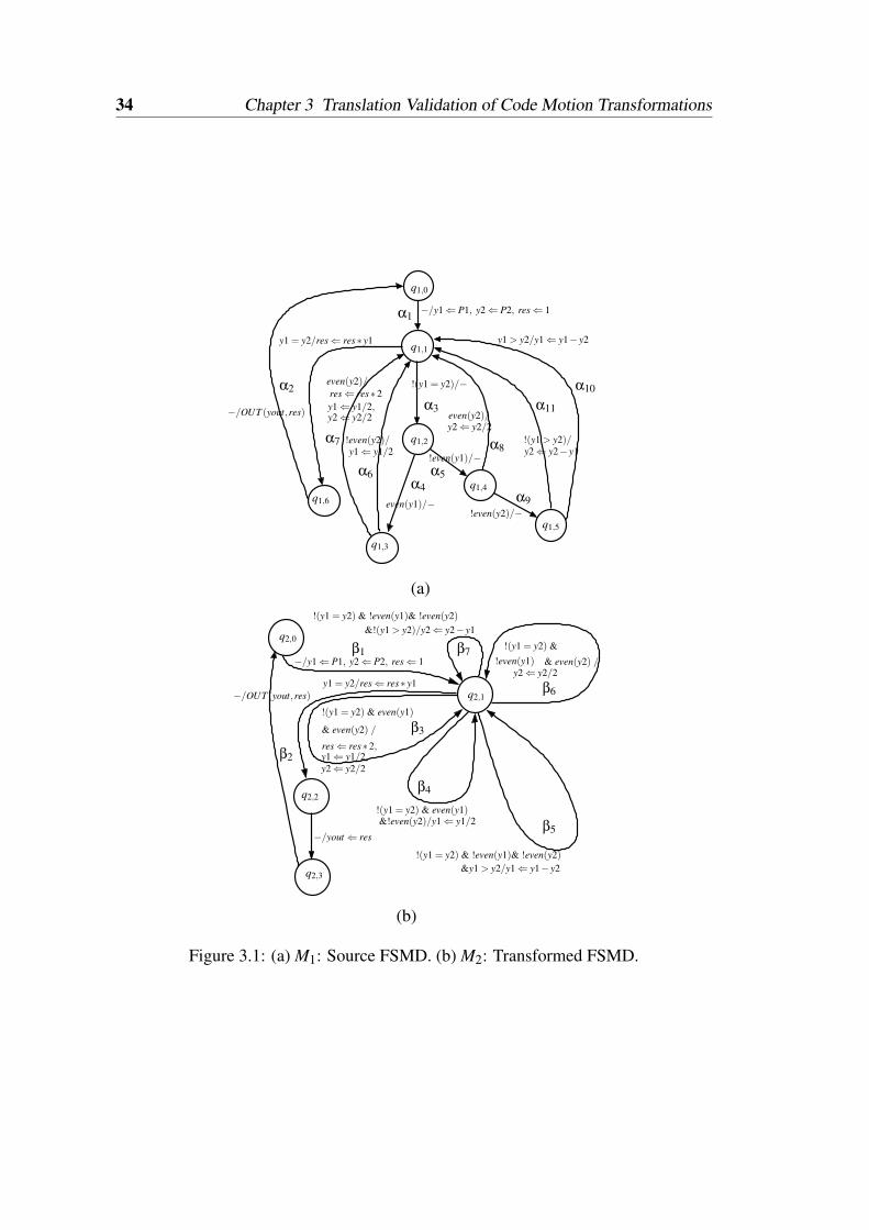
34 Chapter 3 Translation Validation of Code Motion Transformations
even(y2)/
!even(y2)/
even(y1)/−!even(y2)/−
even(y2)/
y1⇐ y1/2
y2⇐ y2/2
y1⇐ y1/2,y2⇐ y2/2
!(y1 = y2)/−
!even(y1)/−
!(y1 > y2)/
y1 > y2/y1⇐ y1− y2
y2⇐ y2− y1
res⇐ res∗2
−/OUT (yout,res)
q1,5
q1,4
q1,2
q1,1
q1,0
−/y1⇐ P1, y2⇐ P2, res⇐ 1
(a)
(b)
y1⇐ y1/2,y2⇐ y2/2
!(y1 = y2) & !even(y1)& !even(y2)
−/y1⇐ P1, y2⇐ P2, res⇐ 1
!(y1 = y2) & even(y1)
res⇐ res∗2,
q2,2
!(y1 = y2) &
q2,1
y2⇐ y2/2
!(y1 = y2) & !even(y1)& !even(y2)&y1 > y2/y1⇐ y1− y2
!(y1 = y2) & even(y1)&!even(y2)/y1⇐ y1/2
−/yout⇐ res
y1 = y2/res⇐ res∗ y1
& even(y2) /
!even(y1) & even(y2) /
q2,0
q2,3
&!(y1 > y2)/y2⇐ y2− y1
−/OUT (yout,res)
y1 = y2/res⇐ res∗ y1
q1,6
q1,3
β2
β4
β5
β6
β7
β3
β1
α2
α3
α5α6
α7
α10
α11
α4
α8
α1
α9
Figure 3.1: (a) M1: Source FSMD. (b) M2: Transformed FSMD.
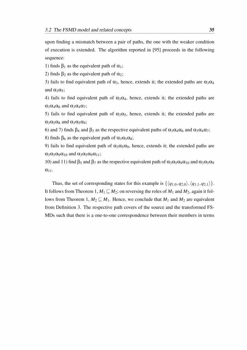
3.2 The FSMD model and related concepts 35
upon finding a mismatch between a pair of paths, the one with the weaker condition
of execution is extended. The algorithm reported in [95] proceeds in the following
sequence:
1) finds β1 as the equivalent path of α1;
2) finds β2 as the equivalent path of α2;
3) fails to find equivalent path of α3, hence, extends it; the extended paths are α3α4
and α3α5;
4) fails to find equivalent path of α3α4, hence, extends it; the extended paths are
α3α4α6 and α3α4α7;
5) fails to find equivalent path of α3α5, hence, extends it; the extended paths are
α3α5α8 and α3α5α9;
6) and 7) finds β4 and β3 as the respective equivalent paths of α3α4α6 and α3α4α7;
8) finds β6 as the equivalent path of α3α5α8;
9) fails to find equivalent path of α3α5α9, hence, extends it; the extended paths are
α3α5α9α10 and α3α5α9α11;
10) and 11) find β5 and β7 as the respective equivalent path of α3α5α9α10 and α3α5α9
α11.
Thus, the set of corresponding states for this example is 〈q1,0,q2,0〉,〈q1,1,q2,1〉.It follows from Theorem 1, M1vM2; on reversing the roles of M1 and M2, again it fol-
lows from Theorem 1, M2 vM1. Hence, we conclude that M1 and M2 are equivalent
from Definition 3. The respective path covers of the source and the transformed FS-
MDs such that there is a one-to-one correspondence between their members in terms
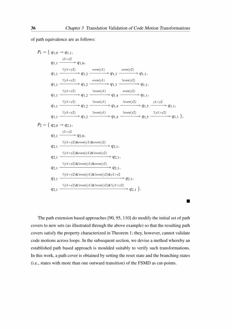
36 Chapter 3 Translation Validation of Code Motion Transformations
of path equivalence are as follows:
P1 = q1,0 q1,1,
q1,1y1=y2−−−−− q1,0,
q1,1!(y1=y2)−−−−−−− q1,2
even(y1)−−−−−− q1,3
even(y2)−−−−−− q1,1,
q1,1!(y1=y2)−−−−−−− q1,2
even(y1)−−−−−− q1,3
!even(y2)−−−−−−− q1,1,
q1,1!(y1=y2)−−−−−−− q1,2
!even(y1)−−−−−−− q1,4
even(y2)−−−−−− q1,1,
q1,1!(y1=y2)−−−−−−− q1,2
!even(y1)−−−−−−− q1,4
!even(y2)−−−−−−− q1,5
y1>y2−−−−− q1,1,
q1,1!(y1=y2)−−−−−−− q1,2
!even(y1)−−−−−−− q1,4
!even(y2)−−−−−−− q1,5
!(y1>y2)−−−−−−− q1,1 ,
P2 = q2,0 q2,1,
q2,1y1=y2−−−−− q2,0,
q2,1!(y1=y2)&even(y1)&even(y2)−−−−−−−−−−−−−−−−−− q2,1,
q2,1!(y1=y2)&even(y1)&!even(y2)−−−−−−−−−−−−−−−−−−− q2,1,
q2,1!(y1=y2)&!even(y1)&even(y2)−−−−−−−−−−−−−−−−−−− q2,1,
q2,1!(y1=y2)&!even(y1)&!even(y2)&y1>y2−−−−−−−−−−−−−−−−−−−−−−−− q2,1,
q2,1!(y1=y2)&!even(y1)&!even(y2)&!(y1>y2)−−−−−−−−−−−−−−−−−−−−−−−−−− q2,1 .
The path extension based approaches [90, 95, 110] do modify the initial set of path
covers to new sets (as illustrated through the above example) so that the resulting path
covers satisfy the property characterized in Theorem 1; they, however, cannot validate
code motions across loops. In the subsequent section, we devise a method whereby an
established path based approach is moulded suitably to verify such transformations.
In this work, a path cover is obtained by setting the reset state and the branching states
(i.e., states with more than one outward transition) of the FSMD as cut-points.
3.3 The method of symbolic value propagation 37
3.3 The method of symbolic value propagation
3.3.1 Basic concepts
The symbolic value propagation method consists in propagating values of variables
over the corresponding paths of the two FSMDs on discovery of mismatch in the val-
ues of some live variable; the mismatched values are marked to distinguish them from
the matched values. A variable v is said to be live at a state s if there is an execution
sequence starting at s along which its value may be used before v is redefined [10].
Propagation of values from a path α1 to the next path α2 is accomplished by asso-
ciating a propagated vector at the end state of the path α1 (or equivalently, the start
state of the path α2). A propagated vector ϑ through a path α1 is an ordered pair
of the form 〈C ,〈e1,e2, · · · ,ek〉〉, where k = |V1⋃
V2|. The first element C of the pair
represents the condition that has to be satisfied at the start state of α1 to traverse the
path and reach its end state with the upgraded propagated vector. The second element,
referred to as value-vector, comprises of ei, 1≤ i≤ k, which represents the symbolic
value attained at the end state of α1 by the variable vi ∈ V1⋃
V2. To start with, for
the reset state, the propagated vector is 〈>,〈v1,v2, · · · ,vk〉〉 (also represented as υ),
where > stands for true and ei = vi,1≤ i≤ k, indicates that the variables are yet to be
defined. For brevity, we represent the second component as v to mean 〈v1,v2, · · · ,vk〉and as e to mean 〈e1,e2, · · · ,ek〉, where ei’s are the symbolic expressions (values) in-
volving variables vi,1 ≤ i ≤ k, in general. It is important to note that an uncommon
variable, i.e., a variable that is defined in either of the FSMDs but not both, from the
set V2−V1 (V1−V2) retains its symbolic value in the propagated vectors of M1 (M2)
throughout a computation of M1 (M2). Let Rα(v) and sα(v) represent respectively
the condition of execution and the data transformation of a path α when there is no
propagated vector at the start state αs of α. In the presence of a propagated vector,
ϑαs = 〈c1,e〉 say, at αs, its condition of execution becomes c1(v)∧Rα(v)e/v and the
data transformation becomes sα(v)e/v, where e/v is called a substitution; the ex-
pression κe/v represents that each variable v j ∈ v that occurs in κ is replaced by the
corresponding expression e j ∈ e simultaneously with other variables. The propagated
vector ϑα associated with a path α : αs α f will synonymously be referred to as
ϑα f associated with the final state α f of α. Also, we use the symbol ϑi, j to represent
a propagated vector corresponding to the state qi, j. We follow a similar convention
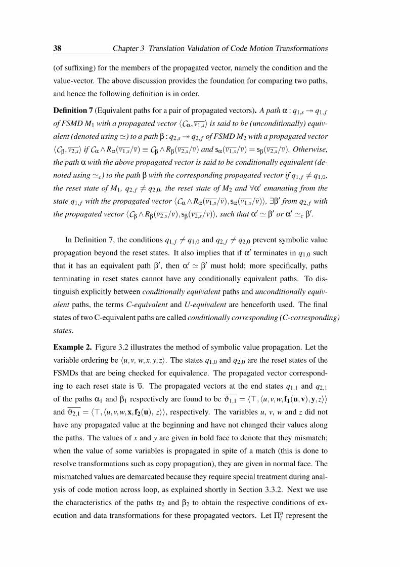
38 Chapter 3 Translation Validation of Code Motion Transformations
(of suffixing) for the members of the propagated vector, namely the condition and the
value-vector. The above discussion provides the foundation for comparing two paths,
and hence the following definition is in order.
Definition 7 (Equivalent paths for a pair of propagated vectors). A path α : q1,s q1, f
of FSMD M1 with a propagated vector 〈Cα,v1,s〉 is said to be (unconditionally) equiv-
alent (denoted using') to a path β : q2,s q2, f of FSMD M2 with a propagated vector
〈Cβ,v2,s〉 if Cα∧Rα(v1,s/v)≡ Cβ∧Rβ(v2,s/v) and sα(v1,s/v) = sβ(v2,s/v). Otherwise,
the path α with the above propagated vector is said to be conditionally equivalent (de-
noted using 'c) to the path β with the corresponding propagated vector if q1, f 6= q1,0,
the reset state of M1, q2, f 6= q2,0, the reset state of M2 and ∀α′ emanating from the
state q1, f with the propagated vector 〈Cα∧Rα(v1,s/v),sα(v1,s/v)〉, ∃β′ from q2, f with
the propagated vector 〈Cβ∧Rβ(v2,s/v),sβ(v2,s/v)〉, such that α′ ' β′ or α′ 'c β′.
In Definition 7, the conditions q1, f 6= q1,0 and q2, f 6= q2,0 prevent symbolic value
propagation beyond the reset states. It also implies that if α′ terminates in q1,0 such
that it has an equivalent path β′, then α′ ' β′ must hold; more specifically, paths
terminating in reset states cannot have any conditionally equivalent paths. To dis-
tinguish explicitly between conditionally equivalent paths and unconditionally equiv-
alent paths, the terms C-equivalent and U-equivalent are henceforth used. The final
states of two C-equivalent paths are called conditionally corresponding (C-corresponding)
states.
Example 2. Figure 3.2 illustrates the method of symbolic value propagation. Let the
variable ordering be 〈u,v, w,x,y,z〉. The states q1,0 and q2,0 are the reset states of the
FSMDs that are being checked for equivalence. The propagated vector correspond-
ing to each reset state is υ. The propagated vectors at the end states q1,1 and q2,1
of the paths α1 and β1 respectively are found to be ϑ1,1 = 〈>,〈u,v,w, f1(u,v),y,z〉〉and ϑ2,1 = 〈>,〈u,v,w,x, f2(u), z〉〉, respectively. The variables u, v, w and z did not
have any propagated value at the beginning and have not changed their values along
the paths. The values of x and y are given in bold face to denote that they mismatch;
when the value of some variables is propagated in spite of a match (this is done to
resolve transformations such as copy propagation), they are given in normal face. The
mismatched values are demarcated because they require special treatment during anal-
ysis of code motion across loop, as explained shortly in Section 3.3.2. Next we use
the characteristics of the paths α2 and β2 to obtain the respective conditions of ex-
ecution and data transformations for these propagated vectors. Let Πni represent the
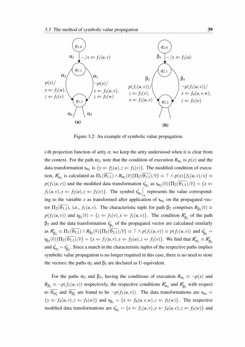
3.3 The method of symbolic value propagation 39
−/x⇐ f1(u,v)
¬p(x)/
q1,0
q1,1
q1,2
α3α2
α1
(a)
α5α4
z⇐ f3(v)y⇐ f2(u),
p(x)/
z⇐ f5(w)y⇐ f4(u,v),
p( f1(u,v))/z⇐ f3(v),x⇐ f1(u,v)
q2,0
q2,1
q2,2
−/y⇐ f2(u)β1
(b)
¬p( f1(u,v))/
β3
x⇐ f6(u,v,w),
z⇐ f5(w)
β2
Figure 3.2: An example of symbolic value propagation.
i-th projection function of arity n; we keep the arity understood when it is clear from
the context. For the path α2, note that the condition of execution Rα2 is p(x) and the
data transformation sα2 is y⇐ f2(u),z⇐ f3(v). The modified condition of execu-
tion, R′α2is calculated as Π1(ϑ1,1)∧Rα2(v)Π2(ϑ1,1)/v ≡ >∧ p(x) f1(u,v)/x ≡
p( f1(u,v)) and the modified data transformation s′α2as sα2(v)Π2(ϑ1,1)/v = x⇐
f1(u,v),y⇐ f2(u),z⇐ f3(v). The symbol s′α2
∣∣∣x
represents the value correspond-
ing to the variable x as transformed after application of sα2 on the propagated vec-
tor Π2(ϑ1,1), i.e., f1(u,v). The characteristic tuple for path β2 comprises Rβ2(v) ≡p( f1(u,v)) and sβ2(v) = z⇐ f3(v),x⇐ f1(u,v). The condition R′
β2of the path
β2 and the data transformation s′β2
of the propagated vector are calculated similarly
as R′β2≡ Π1(ϑ2,1)∧Rβ2(v)Π2(ϑ2,1)/v ≡ >∧ p( f1(u,v)) ≡ p( f1(u,v)) and s′
β2=
sβ2(v)Π2(ϑ2,1)/v = x⇐ f1(u,v),y⇐ f2(u),z⇐ f3(v). We find that R′α2≡ R′
β2
and s′α2= s′
β2. Since a match in the characteristic tuples of the respective paths implies
symbolic value propagation is no longer required in this case, there is no need to store
the vectors; the paths α2 and β2 are declared as U-equivalent.
For the paths α3 and β3, having the conditions of execution Rα3 ≡ ¬p(x) and
Rβ3 ≡ ¬p( f1(u,v)) respectively, the respective conditions R′α3and R′
β3with respect
to ϑαs3
and ϑβs3
are found to be ¬p( f1(u,v)). The data transformations are sα3 =
y ⇐ f4(u,v),z ⇐ f5(w) and sβ3 = x ⇐ f6(u,v,w),z ⇐ f5(w). The respective
modified data transformations are s′α3= x⇐ f1(u,v),y⇐ f4(u,v),z⇐ f5(w) and
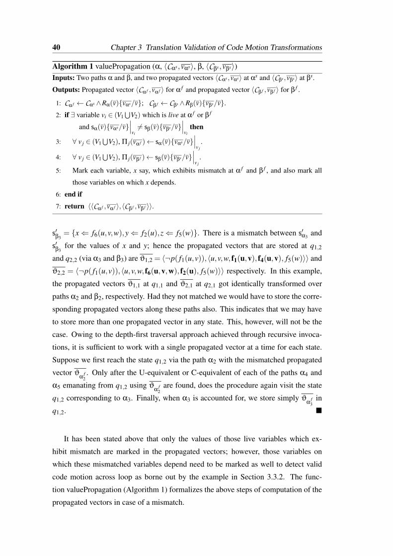
40 Chapter 3 Translation Validation of Code Motion Transformations
Algorithm 1 valuePropagation (α, 〈Cαs,vαs〉, β, 〈Cβs,vβs〉)Inputs: Two paths α and β, and two propagated vectors 〈Cαs ,vαs〉 at αs and 〈Cβs ,vβs〉 at βs.
Outputs: Propagated vector 〈Cα f ,vα f 〉 for α f and propagated vector 〈Cβ f ,vβ f 〉 for β f .
1: Cα f ← Cαs ∧Rα(v)vαs/v; Cβ f ← Cβs ∧Rβ(v)vβs/v.2: if ∃ variable vi ∈ (V1
⋃V2) which is live at α f or β f
and sα(v)vαs/v∣∣∣vi6= sβ(v)vβs/v
∣∣∣vi
then
3: ∀ v j ∈ (V1⋃
V2), Π j(vα f )← sα(v)vαs/v∣∣∣v j
.
4: ∀ v j ∈ (V1⋃
V2), Π j(vβ f )← sβ(v)vβs/v∣∣∣v j
.
5: Mark each variable, x say, which exhibits mismatch at α f and β f , and also mark all
those variables on which x depends.
6: end if
7: return 〈〈Cα f ,vα f 〉,〈Cβ f ,vβ f 〉〉.
s′β3
= x⇐ f6(u,v,w),y⇐ f2(u),z⇐ f5(w). There is a mismatch between s′α3and
s′β3
for the values of x and y; hence the propagated vectors that are stored at q1,2
and q2,2 (via α3 and β3) are ϑ1,2 = 〈¬p( f1(u,v)),〈u,v,w, f1(u,v), f4(u,v), f5(w)〉〉 and
ϑ2,2 = 〈¬p( f1(u,v)),〈u,v,w, f6(u,v,w), f2(u), f5(w)〉〉 respectively. In this example,
the propagated vectors ϑ1,1 at q1,1 and ϑ2,1 at q2,1 got identically transformed over
paths α2 and β2, respectively. Had they not matched we would have to store the corre-
sponding propagated vectors along these paths also. This indicates that we may have
to store more than one propagated vector in any state. This, however, will not be the
case. Owing to the depth-first traversal approach achieved through recursive invoca-
tions, it is sufficient to work with a single propagated vector at a time for each state.
Suppose we first reach the state q1,2 via the path α2 with the mismatched propagated
vector ϑα
f2. Only after the U-equivalent or C-equivalent of each of the paths α4 and
α5 emanating from q1,2 using ϑα
f2
are found, does the procedure again visit the state
q1,2 corresponding to α3. Finally, when α3 is accounted for, we store simply ϑα
f3
in
q1,2.
It has been stated above that only the values of those live variables which ex-
hibit mismatch are marked in the propagated vectors; however, those variables on
which these mismatched variables depend need to be marked as well to detect valid
code motion across loop as borne out by the example in Section 3.3.2. The func-
tion valuePropagation (Algorithm 1) formalizes the above steps of computation of the
propagated vectors in case of a mismatch.
3.3 The method of symbolic value propagation 41
Using symbolic value propagation as a pivotal concept, we need to formalize our
main task of equivalence checking of two given FSMDs. However, certain intricacies
are interlaced with symbolic value propagation which need to be resolved first. The
following subsections illustrate these intricacies and furnishes the mechanisms for
addressing them. The overall verification method is then presented in a subsequent
section.
3.3.2 Need for detecting loop invariance of subexpressions
In order to verify behaviours in the presence of code motions beyond loops, one needs
to ascertain whether certain subexpressions remain invariants in a loop or not. Ba-
sically, suppose some variable, w say, gets defined before a loop L in the original
behaviour, and somehow it can be confirmed that the value of w remains invariant
in that loop. Now, if an equivalent definition for w is found in the other behaviour
after exiting the loop L′ (which corresponds to L), then such behaviours will indeed
be equivalent. In this work, we target to establish the loop invariance of propagated
vectors which, in turn, suffices to prove the loop invariance of the involved variables.
The following example is used to reveal these facts more vividly.
q1,2
−/i⇐ 1,y⇐ t1− t2
¬i < N/−
q1,0
〈T,〈x,y,1,N, t1, t2, t1+ t2〉〉
q2,0
q2,2
¬i < N/y⇐ t1− t2
−/i⇐ 1,h⇐ t1+ t2,
(a) M1 (b) M2
〈T,〈x, t1− t2, i,N, t1, t2, t1+ t2〉〉
〈T,〈x,y, i,N, t1, t2,h〉〉〈T,〈x,y, i,N, t1, t2,h〉〉
q1,1 q2,1
〈T,〈x, t1− t2, i,N, t1, t2,h〉〉
〈T,〈x, t1− t2,1,N, t1, t2,h〉〉
i < N/x⇐ t1+ t2+ x∗ i,i⇐ i+1
i < N/
i⇐ i+1x⇐ h0 + x∗ i,
Figure 3.3: An example of propagation of values across loop.
Example 3. In Figure 3.3, the operation y⇐ t1− t2, which is originally placed before
the loop body in M1 (Figure 3.3(a)), is moved after the loop in the transformed FSMD
M2 (Figure 3.3(b)). This transformation reduces the register lifetime for y. In addition,
the subexpression t1+ t2, which is originally computed in every iteration of the loop,
is now computed only once before the start of the loop and the result is stored in an
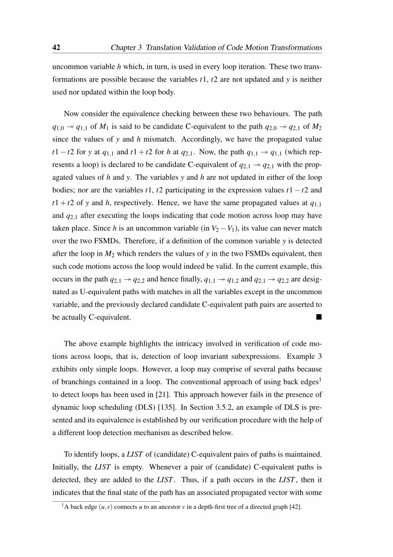
42 Chapter 3 Translation Validation of Code Motion Transformations
uncommon variable h which, in turn, is used in every loop iteration. These two trans-
formations are possible because the variables t1, t2 are not updated and y is neither
used nor updated within the loop body.
Now consider the equivalence checking between these two behaviours. The path
q1,0 q1,1 of M1 is said to be candidate C-equivalent to the path q2,0 q2,1 of M2
since the values of y and h mismatch. Accordingly, we have the propagated value
t1− t2 for y at q1,1 and t1+ t2 for h at q2,1. Now, the path q1,1 q1,1 (which rep-
resents a loop) is declared to be candidate C-equivalent of q2,1 q2,1 with the prop-
agated values of h and y. The variables y and h are not updated in either of the loop
bodies; nor are the variables t1, t2 participating in the expression values t1− t2 and
t1+ t2 of y and h, respectively. Hence, we have the same propagated values at q1,1
and q2,1 after executing the loops indicating that code motion across loop may have
taken place. Since h is an uncommon variable (in V2−V1), its value can never match
over the two FSMDs. Therefore, if a definition of the common variable y is detected
after the loop in M2 which renders the values of y in the two FSMDs equivalent, then
such code motions across the loop would indeed be valid. In the current example, this
occurs in the path q2,1 q2,2 and hence finally, q1,1 q1,2 and q2,1 q2,2 are desig-
nated as U-equivalent paths with matches in all the variables except in the uncommon
variable, and the previously declared candidate C-equivalent path pairs are asserted to
be actually C-equivalent.
The above example highlights the intricacy involved in verification of code mo-
tions across loops, that is, detection of loop invariant subexpressions. Example 3
exhibits only simple loops. However, a loop may comprise of several paths because
of branchings contained in a loop. The conventional approach of using back edges1
to detect loops has been used in [21]. This approach however fails in the presence of
dynamic loop scheduling (DLS) [135]. In Section 3.5.2, an example of DLS is pre-
sented and its equivalence is established by our verification procedure with the help of
a different loop detection mechanism as described below.
To identify loops, a LIST of (candidate) C-equivalent pairs of paths is maintained.
Initially, the LIST is empty. Whenever a pair of (candidate) C-equivalent paths is
detected, they are added to the LIST . Thus, if a path occurs in the LIST , then it
indicates that the final state of the path has an associated propagated vector with some1A back edge (u,v) connects u to an ancestor v in a depth-first tree of a directed graph [42].
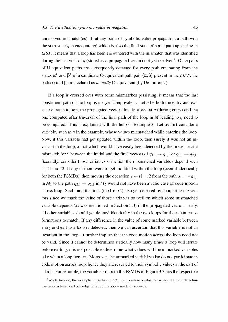
3.3 The method of symbolic value propagation 43
unresolved mismatch(es). If at any point of symbolic value propagation, a path with
the start state q is encountered which is also the final state of some path appearing in
LIST , it means that a loop has been encountered with the mismatch that was identified
during the last visit of q (stored as a propagated vector) not yet resolved2. Once pairs
of U-equivalent paths are subsequently detected for every path emanating from the
states α f and β f of a candidate C-equivalent path pair 〈α,β〉 present in the LIST , the
paths α and β are declared as actually C-equivalent (by Definition 7).
If a loop is crossed over with some mismatches persisting, it means that the last
constituent path of the loop is not yet U-equivalent. Let q be both the entry and exit
state of such a loop; the propagated vector already stored at q (during entry) and the
one computed after traversal of the final path of the loop in M leading to q need to
be compared. This is explained with the help of Example 3. Let us first consider a
variable, such as y in the example, whose values mismatched while entering the loop.
Now, if this variable had got updated within the loop, then surely it was not an in-
variant in the loop, a fact which would have easily been detected by the presence of a
mismatch for y between the initial and the final vectors of q1,1 q1,1 or q2,1 q2,1.
Secondly, consider those variables on which the mismatched variables depend such
as, t1 and t2. If any of them were to get modified within the loop (even if identically
for both the FSMDs), then moving the operation y⇐ t1− t2 from the path q1,0 q1,1
in M1 to the path q2,1 q2,2 in M2 would not have been a valid case of code motion
across loop. Such modifications (in t1 or t2) also get detected by comparing the vec-
tors since we mark the value of those variables as well on which some mismatched
variable depends (as was mentioned in Section 3.3) in the propagated vector. Lastly,
all other variables should get defined identically in the two loops for their data trans-
formations to match. If any difference in the value of some marked variable between
entry and exit to a loop is detected, then we can ascertain that this variable is not an
invariant in the loop. It further implies that the code motion across the loop need not
be valid. Since it cannot be determined statically how many times a loop will iterate
before exiting, it is not possible to determine what values will the unmarked variables
take when a loop iterates. Moreover, the unmarked variables also do not participate in
code motion across loop, hence they are reverted to their symbolic values at the exit of
a loop. For example, the variable i in both the FSMDs of Figure 3.3 has the respective
2While treating the example in Section 3.5.2, we underline a situation where the loop detection
mechanism based on back edge fails and the above method succeeds.
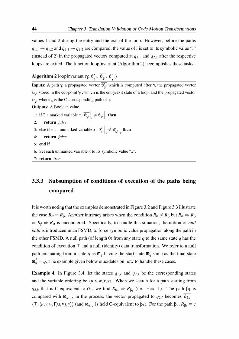
44 Chapter 3 Translation Validation of Code Motion Transformations
values 1 and 2 during the entry and the exit of the loop. However, before the paths
q1,1 q1,2 and q2,1 q2,2 are compared, the value of i is set to its symbolic value “i”
(instead of 2) in the propagated vectors computed at q1,1 and q2,1 after the respective
loops are exited. The function loopInvariant (Algorithm 2) accomplishes these tasks.
Algorithm 2 loopInvariant (γ, ϑ′γ f , ϑγ f , ϑ′
ς f )
Inputs: A path γ, a propagated vector ϑ′γ f which is computed after γ, the propagated vector
ϑγ f stored in the cut-point γ f , which is the entry/exit state of a loop, and the propagated vector
ϑ′ς f where ς is the C-corresponding path of γ.
Outputs: A Boolean value.
1: if ∃ a marked variable x, ϑ′γ f
∣∣∣x6= ϑγ f
∣∣∣x
then
2: return false.
3: else if ∃ an unmarked variable x, ϑ′γ f
∣∣∣x6= ϑ′
ς f
∣∣∣x
then
4: return false.
5: end if
6: Set each unmarked variable x to its symbolic value “x”.
7: return true.
3.3.3 Subsumption of conditions of execution of the paths being
compared
It is worth noting that the examples demonstrated in Figure 3.2 and Figure 3.3 illustrate
the case Rα ≡ Rβ. Another intricacy arises when the condition Rα 6≡ Rβ but Rα⇒ Rβ
or Rβ ⇒ Rα is encountered. Specifically, to handle this situation, the notion of null
path is introduced in an FSMD, to force symbolic value propagation along the path in
the other FSMD. A null path (of length 0) from any state q to the same state q has the
condition of execution > and a null (identity) data transformation. We refer to a null
path emanating from a state q as ϖq having the start state ϖsq same as the final state
ϖfq = q. The example given below elucidates on how to handle these cases.
Example 4. In Figure 3.4, let the states q1,r and q2,k be the corresponding states
and the variable ordering be 〈u,v,w,x,y〉. When we search for a path starting from
q2,k that is C-equivalent to α1, we find Rα1 ⇒ Rβ1 (i.e. c ⇒ >). The path β1 is
compared with ϖq1,r ; in the process, the vector propagated to q2,l becomes ϑ2,l =
〈>,〈u,v,w, f(u,v),y〉〉 (and ϖq1,r is held C-equivalent to β1). For the path β2, Rβ2 ≡ c
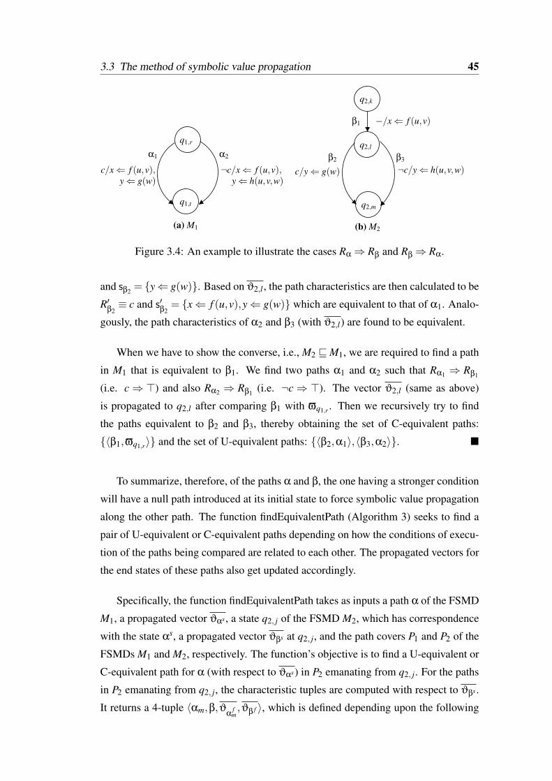
3.3 The method of symbolic value propagation 45
α1
y⇐ h(u,v,w)
α2
q1,r
q1,t
β1
q2,k
q2,l
q2,m
¬c/y⇐ h(u,v,w)β3β2
−/x⇐ f (u,v)
(a) M1 (b) M2
¬c/x⇐ f (u,v), c/y⇐ g(w)c/x⇐ f (u,v),y⇐ g(w)
Figure 3.4: An example to illustrate the cases Rα⇒ Rβ and Rβ⇒ Rα.
and sβ2 = y⇐ g(w). Based on ϑ2,l , the path characteristics are then calculated to be
R′β2≡ c and s′
β2= x⇐ f (u,v),y⇐ g(w) which are equivalent to that of α1. Analo-
gously, the path characteristics of α2 and β3 (with ϑ2,l) are found to be equivalent.
When we have to show the converse, i.e., M2 vM1, we are required to find a path
in M1 that is equivalent to β1. We find two paths α1 and α2 such that Rα1 ⇒ Rβ1
(i.e. c⇒ >) and also Rα2 ⇒ Rβ1 (i.e. ¬c⇒ >). The vector ϑ2,l (same as above)
is propagated to q2,l after comparing β1 with ϖq1,r . Then we recursively try to find
the paths equivalent to β2 and β3, thereby obtaining the set of C-equivalent paths:
〈β1,ϖq1,r〉 and the set of U-equivalent paths: 〈β2,α1〉,〈β3,α2〉.
To summarize, therefore, of the paths α and β, the one having a stronger condition
will have a null path introduced at its initial state to force symbolic value propagation
along the other path. The function findEquivalentPath (Algorithm 3) seeks to find a
pair of U-equivalent or C-equivalent paths depending on how the conditions of execu-
tion of the paths being compared are related to each other. The propagated vectors for
the end states of these paths also get updated accordingly.
Specifically, the function findEquivalentPath takes as inputs a path α of the FSMD
M1, a propagated vector ϑαs , a state q2, j of the FSMD M2, which has correspondence
with the state αs, a propagated vector ϑβs at q2, j, and the path covers P1 and P2 of the
FSMDs M1 and M2, respectively. The function’s objective is to find a U-equivalent or
C-equivalent path for α (with respect to ϑαs) in P2 emanating from q2, j. For the paths
in P2 emanating from q2, j, the characteristic tuples are computed with respect to ϑβs .
It returns a 4-tuple 〈αm,β,ϑα
fm,ϑβ f 〉, which is defined depending upon the following
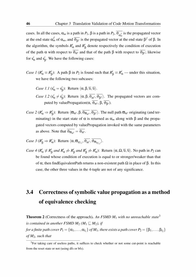
46 Chapter 3 Translation Validation of Code Motion Transformations
cases. In all the cases, αm is a path in P1, β is a path in P2, ϑα
fm
is the propagated vector
at the end state αfm of αm, and ϑβ f is the propagated vector at the end state β f of β. In
the algorithm, the symbols R′α and R′β
denote respectively the condition of execution
of the path α with respect to ϑαs and that of the path β with respect to ϑβs; likewise
for s′α and s′β. We have the following cases:
Case 1 (R′α ≡ R′β): A path β in P2 is found such that R′
β≡ R′α — under this situation,
we have the following two subcases:
Case 1.1 (s′α = s′β): Return 〈α,β,υ,υ〉.
Case 1.2 (s′α 6= s′β): Return 〈α,β,ϑα f ,ϑβ f 〉. The propagated vectors are com-
puted by valuePropagation(α, ϑαs , β, ϑβs).
Case 2 (R′α⇒ R′β): Return 〈ϖαs,β,ϑϖαs ,ϑβ f 〉. The null path ϖαs originating (and ter-
minating) in the start state of α is returned as αm along with β and the propa-
gated vectors computed by valuePropagation invoked with the same parameters
as above. Note that ϑϖαs = ϑαs .
Case 3 (R′β⇒ R′α): Return 〈α,ϖq2, j ,ϑα f ,ϑϖq2, j
〉.
Case 4 (R′α 6≡ R′β
and R′α 6⇒ R′β
and R′β6⇒ R′α): Return 〈α,Ω,υ,υ〉. No path in P2 can
be found whose condition of execution is equal to or stronger/weaker than that
of α; then findEquivalentPath returns a non-existent path Ω in place of β. In this
case, the other three values in the 4-tuple are not of any significance.
3.4 Correctness of symbolic value propagation as a method
of equivalence checking
Theorem 2 (Correctness of the approach). An FSMD M1 with no unreachable state3
is contained in another FSMD M2 (M1 vM2), if
for a finite path cover P1 = α1, . . . ,αl1 of M1, there exists a path cover P2 = β1, . . . ,βl2of M2, such that
3For taking care of useless paths, it suffices to check whether or not some cut-point is reachable
from the reset state or not (using dfs or bfs).
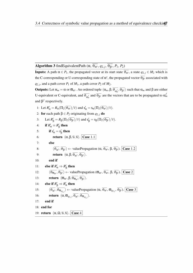
3.4 Correctness of symbolic value propagation as a method of equivalence checking47
Algorithm 3 findEquivalentPath (α, ϑαs , q2, j, ϑβs , P1, P2)
Inputs: A path α ∈ P1, the propagated vector at its start state ϑαs , a state q2, j ∈M2 which is
the C-corresponding or U-corresponding state of αs, the propagated vector ϑβs associated with
q2, j, and a path cover P1 of M1, a path cover P2 of M2.
Outputs: Let αm = α or ϖαs . An ordered tuple 〈αm,β,ϑαfm,ϑβ f 〉 such that αm and β are either
U-equivalent or C-equivalent, and ϑα
fm
and ϑβ f are the vectors that are to be propagated to αfm
and β f respectively.
1: Let R′α = Rα(Π2(ϑαs)/v) and s′α = sα(Π2(ϑαs)/v).
2: for each path β ∈ P2 originating from q2, j do
3: Let R′β= Rβ(Π2(ϑβs)/v) and s′
β= sβ(Π2(ϑβs)/v).
4: if R′α ≡ R′β
then
5: if s′α = s′β
then
6: return 〈α,β,υ,υ〉. Case 1.1
7: else
8: 〈ϑα f ,ϑβ f 〉 ← valuePropagation (α, ϑαs , β, ϑβs). Case 1.2
9: return 〈α,β,ϑα f ,ϑβ f 〉.10: end if
11: else if R′α⇒ R′β
then
12: 〈ϑϖαs ,ϑβ f 〉 ← valuePropagation (ϖαs , ϑαs , β, ϑβs). Case 2
13: return 〈ϖαs ,β,ϑϖαs ,ϑβ f 〉.14: else if R′
β⇒ R′α then
15: 〈ϑα f ,ϑϖq2, j〉 ← valuePropagation (α, ϑαs , ϖq2, j , ϑβs). Case 3
16: return 〈α,ϖq2, j ,ϑα f ,ϑϖq2, j〉.
17: end if
18: end for
19: return 〈α,Ω,υ,υ〉. Case 4
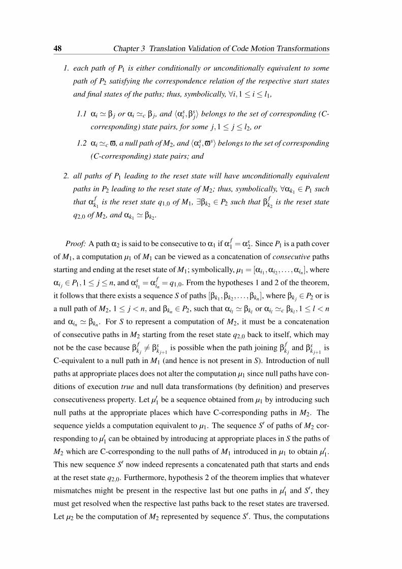
48 Chapter 3 Translation Validation of Code Motion Transformations
1. each path of P1 is either conditionally or unconditionally equivalent to some
path of P2 satisfying the correspondence relation of the respective start states
and final states of the paths; thus, symbolically, ∀i,1≤ i≤ l1,
1.1 αi ' β j or αi 'c β j, and 〈αsi ,β
sj〉 belongs to the set of corresponding (C-
corresponding) state pairs, for some j,1≤ j ≤ l2, or
1.2 αi'c ϖ, a null path of M2, and 〈αsi ,ϖ
s〉 belongs to the set of corresponding
(C-corresponding) state pairs; and
2. all paths of P1 leading to the reset state will have unconditionally equivalent
paths in P2 leading to the reset state of M2; thus, symbolically, ∀αk1 ∈ P1 such
that αfk1
is the reset state q1,0 of M1, ∃βk2 ∈ P2 such that βfk2
is the reset state
q2,0 of M2, and αk1 ' βk2 .
Proof: A path α2 is said to be consecutive to α1 if αf1 =αs
2. Since P1 is a path cover
of M1, a computation µ1 of M1 can be viewed as a concatenation of consecutive paths
starting and ending at the reset state of M1; symbolically, µ1 = [αi1 ,αi2, . . . ,αin], where
αi j ∈ P1,1≤ j≤ n, and αsi1 = α
fin = q1,0. From the hypotheses 1 and 2 of the theorem,
it follows that there exists a sequence S of paths [βk1,βk2, . . . ,βkn ], where βk j ∈ P2 or is
a null path of M2, 1≤ j < n, and βkn ∈ P2, such that αil ' βkl or αil 'c βkl ,1≤ l < n
and αin ' βkn . For S to represent a computation of M2, it must be a concatenation
of consecutive paths in M2 starting from the reset state q2,0 back to itself, which may
not be the case because βfk j6= βs
k j+1is possible when the path joining β
fk j
and βsk j+1
is
C-equivalent to a null path in M1 (and hence is not present in S). Introduction of null
paths at appropriate places does not alter the computation µ1 since null paths have con-
ditions of execution true and null data transformations (by definition) and preserves
consecutiveness property. Let µ′1 be a sequence obtained from µ1 by introducing such
null paths at the appropriate places which have C-corresponding paths in M2. The
sequence yields a computation equivalent to µ1. The sequence S′ of paths of M2 cor-
responding to µ′1 can be obtained by introducing at appropriate places in S the paths of
M2 which are C-corresponding to the null paths of M1 introduced in µ1 to obtain µ′1.
This new sequence S′ now indeed represents a concatenated path that starts and ends
at the reset state q2,0. Furthermore, hypothesis 2 of the theorem implies that whatever
mismatches might be present in the respective last but one paths in µ′1 and S′, they
must get resolved when the respective last paths back to the reset states are traversed.
Let µ2 be the computation of M2 represented by sequence S′. Thus, the computations
3.5 The overall verification method 49
µ2 and µ′1, and hence µ1, must be equivalent.
3.5 The overall verification method
To begin with the procedure of equivalence checking, we have to identify the cut-
points in an FSMD followed by identification of paths and their corresponding char-
acteristics involving the conditions and the data transformations. We also need to
store the pairs of corresponding states in a structure, δ say, and the U-equivalent and
the C-equivalent pairs of paths in Eu and Ec, respectively.
The function containmentChecker (Algorithm 4) initializes all the above men-
tioned data structures, invokes correspondenceChecker (Algorithm 5) with the mem-
bers of the set δ of the corresponding state pairs one by one to check whether for
every path emanating from a state in the pair, there is a U-equivalent or C-equivalent
path from the other member of the pair; depending on the result returned by corre-
spondenceChecker, it outputs the decision whether the original FSMD is contained
in the transformed FSMD or not. A list, called LIST , is maintained to keep track of
the (candidate) C-equivalent pairs of paths visited along the chain of recursive invoca-
tions of correspondenceChecker invoked by containmentChecker. In case the equiva-
lence checking procedure fails for a chain of paths, this LIST is output as a possible
counterexample. Hence, note that every time correspondenceChecker is called from
containmentChecker, the former’s last parameter LIST is set to empty.
The verification procedure starts with the two reset states declared as correspond-
ing states and also ends with the reset states as a corresponding state pair in case the
two FSMDs are indeed equivalent. Otherwise, it terminates on encountering any of
the following “failure” conditions: (i) given a path in one FSMD, it fails to discover its
U-equivalent or C-equivalent path in the other one; (ii) it discovers that a propagated
vector depicting some mismatches at a loop state is not a loop invariant and some of
them do not get resolved in the loop. Note that while failure to find a U-equivalent
path occurs in one step, failure to find a C-equivalent path may be detected only when
the reset state is reached through several steps without finding a match in the variable
values. A chain of C-equivalence may be obtained in the form α1 'c β1 if α2 'c if
α3 'c β3, . . . , if αk ' βk, where αfk and β
fk are the reset states; when αk ' βk is identi-
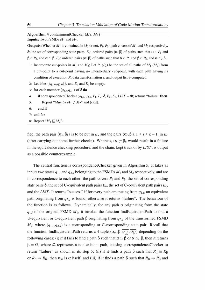
50 Chapter 3 Translation Validation of Code Motion Transformations
Algorithm 4 containmentChecker (M1, M2)Inputs: Two FSMDs M1 and M2.
Outputs: Whether M1 is contained in M2 or not, P1, P2: path covers of M1 and M2 respectively,
δ: the set of corresponding state pairs, Eu: ordered pairs 〈α,β〉 of paths such that α ∈ P1 and
β ∈ P2, and α' β, Ec: ordered pairs 〈α,β〉 of paths such that α ∈ P1 and β ∈ P2, and α'c β.
1: Incorporate cut-points in M1 and M2; Let P1 (P2) be the set of all paths of M1 (M2) from
a cut-point to a cut-point having no intermediary cut-point, with each path having its
condition of execution R, data transformation s, and output list θ computed.
2: Let δ be 〈q1,0,q2,0〉, and Eu and Ec be empty.
3: for each member 〈q1,i,q2, j〉 of δ do
4: if correspondenceChecker (q1,i, q2, j, P1, P2, δ, Eu, Ec, LIST =Φ) returns “failure” then
5: Report “May be M1 6vM2” and (exit).
6: end if
7: end for
8: Report “M1 vM2”.
fied, the path pair 〈αk,βk〉 is to be put in Eu and the pairs 〈αi,βi〉,1≤ i≤ k−1, in Ec
(after carrying out some further checks). Whereas, αk 6' βk would result in a failure
in the equivalence checking procedure, and the chain, kept track of by LIST , is output
as a possible counterexample.
The central function is correspondenceChecker given in Algorithm 5. It takes as
inputs two states q1,i and q2, j belonging to the FSMDs M1 and M2 respectively, and are
in correspondence to each other; the path covers P1 and P2, the set of corresponding
state pairs δ, the set of U-equivalent path pairs Eu, the set of C-equivalent path pairs Ec,
and the LIST . It returns “success” if for every path emanating from q1,i, an equivalent
path originating from q2, j is found; otherwise it returns “failure”. The behaviour of
the function is as follows. Dynamically, for any path α originating from the state
q1,i of the original FSMD M1, it invokes the function findEquivalentPath to find a
U-equivalent or C-equivalent path β originating from q2, j of the transformed FSMD
M2, where 〈q1,i,q2, j〉 is a corresponding or C-corresponding state pair. Recall that
the function findEquivalentPath returns a 4-tuple 〈αm,β,ϑα
fm,ϑβ f 〉 depending on the
following cases: (i) if it fails to find a path β such that α' β or α'c β, then it returns
β = Ω, where Ω represents a non-existent path, causing correspondenceChecker to
return “failure” as shown in its step 5; (ii) if it finds a path β such that Rα ≡ Rβ
or Rβ⇒ Rα, then αm is α itself; and (iii) if it finds a path β such that Rα⇒ Rβ and
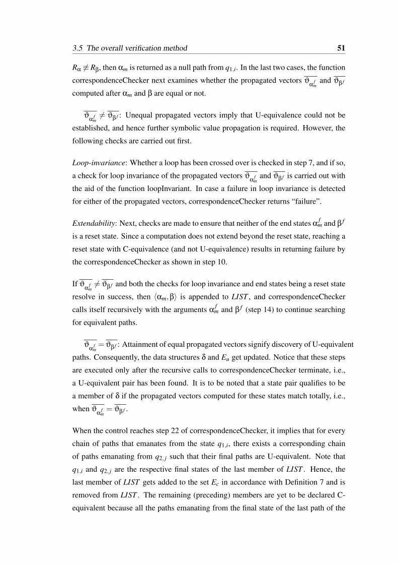
3.5 The overall verification method 51
Rα 6≡ Rβ, then αm is returned as a null path from q1,i. In the last two cases, the function
correspondenceChecker next examines whether the propagated vectors ϑα
fm
and ϑβ f
computed after αm and β are equal or not.
ϑα
fm6= ϑβ f : Unequal propagated vectors imply that U-equivalence could not be
established, and hence further symbolic value propagation is required. However, the
following checks are carried out first.
Loop-invariance: Whether a loop has been crossed over is checked in step 7, and if so,
a check for loop invariance of the propagated vectors ϑα
fm
and ϑβ f is carried out with
the aid of the function loopInvariant. In case a failure in loop invariance is detected
for either of the propagated vectors, correspondenceChecker returns “failure”.
Extendability: Next, checks are made to ensure that neither of the end states αfm and β f
is a reset state. Since a computation does not extend beyond the reset state, reaching a
reset state with C-equivalence (and not U-equivalence) results in returning failure by
the correspondenceChecker as shown in step 10.
If ϑα
fm6= ϑβ f and both the checks for loop invariance and end states being a reset state
resolve in success, then 〈αm,β〉 is appended to LIST , and correspondenceChecker
calls itself recursively with the arguments αfm and β f (step 14) to continue searching
for equivalent paths.
ϑα
fm=ϑβ f : Attainment of equal propagated vectors signify discovery of U-equivalent
paths. Consequently, the data structures δ and Eu get updated. Notice that these steps
are executed only after the recursive calls to correspondenceChecker terminate, i.e.,
a U-equivalent pair has been found. It is to be noted that a state pair qualifies to be
a member of δ if the propagated vectors computed for these states match totally, i.e.,
when ϑα
fm= ϑβ f .
When the control reaches step 22 of correspondenceChecker, it implies that for every
chain of paths that emanates from the state q1,i, there exists a corresponding chain
of paths emanating from q2, j such that their final paths are U-equivalent. Note that
q1,i and q2, j are the respective final states of the last member of LIST . Hence, the
last member of LIST gets added to the set Ec in accordance with Definition 7 and is
removed from LIST . The remaining (preceding) members are yet to be declared C-
equivalent because all the paths emanating from the final state of the last path of the
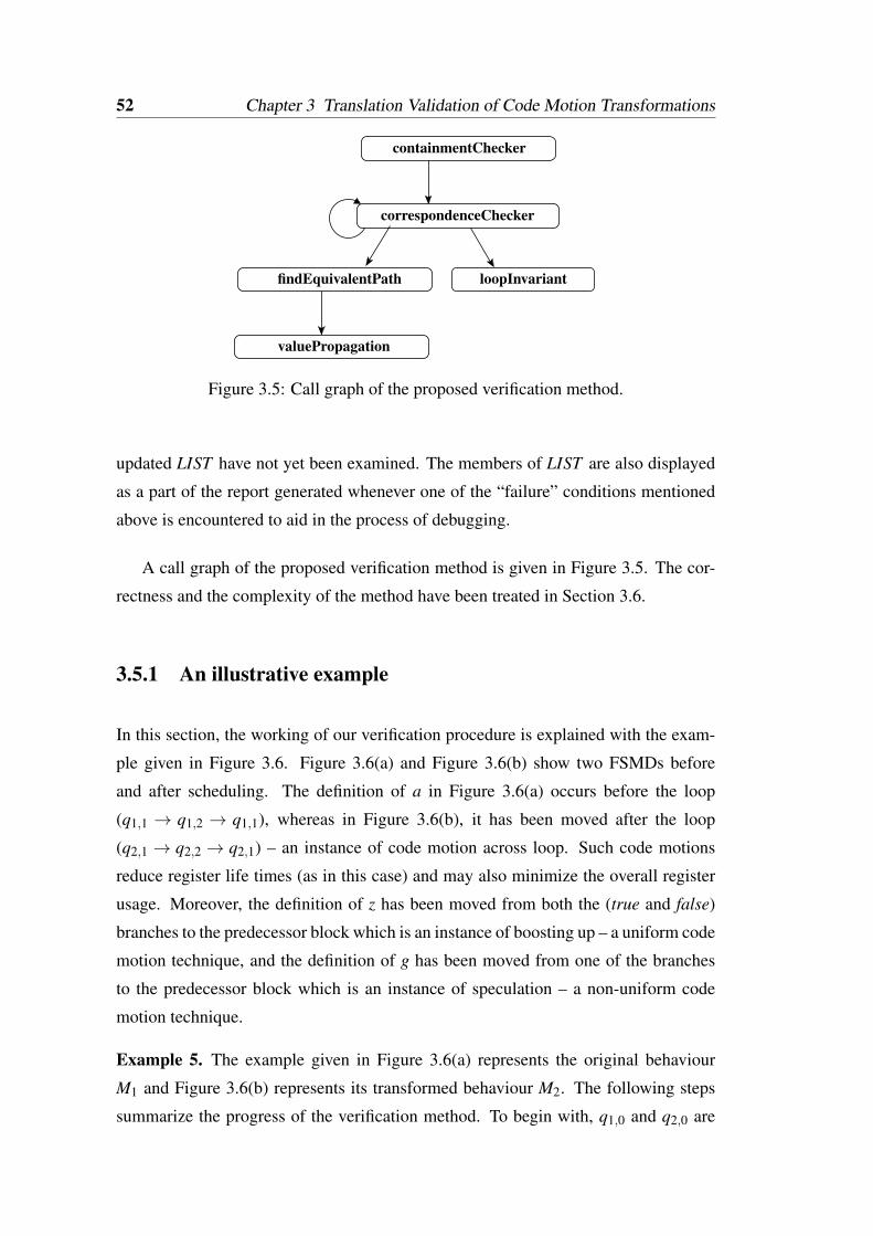
52 Chapter 3 Translation Validation of Code Motion Transformations
containmentChecker
valuePropagation
correspondenceChecker
loopInvariantfindEquivalentPath
Figure 3.5: Call graph of the proposed verification method.
updated LIST have not yet been examined. The members of LIST are also displayed
as a part of the report generated whenever one of the “failure” conditions mentioned
above is encountered to aid in the process of debugging.
A call graph of the proposed verification method is given in Figure 3.5. The cor-
rectness and the complexity of the method have been treated in Section 3.6.
3.5.1 An illustrative example
In this section, the working of our verification procedure is explained with the exam-
ple given in Figure 3.6. Figure 3.6(a) and Figure 3.6(b) show two FSMDs before
and after scheduling. The definition of a in Figure 3.6(a) occurs before the loop
(q1,1 → q1,2 → q1,1), whereas in Figure 3.6(b), it has been moved after the loop
(q2,1 → q2,2 → q2,1) – an instance of code motion across loop. Such code motions
reduce register life times (as in this case) and may also minimize the overall register
usage. Moreover, the definition of z has been moved from both the (true and false)
branches to the predecessor block which is an instance of boosting up – a uniform code
motion technique, and the definition of g has been moved from one of the branches
to the predecessor block which is an instance of speculation – a non-uniform code
motion technique.
Example 5. The example given in Figure 3.6(a) represents the original behaviour
M1 and Figure 3.6(b) represents its transformed behaviour M2. The following steps
summarize the progress of the verification method. To begin with, q1,0 and q2,0 are
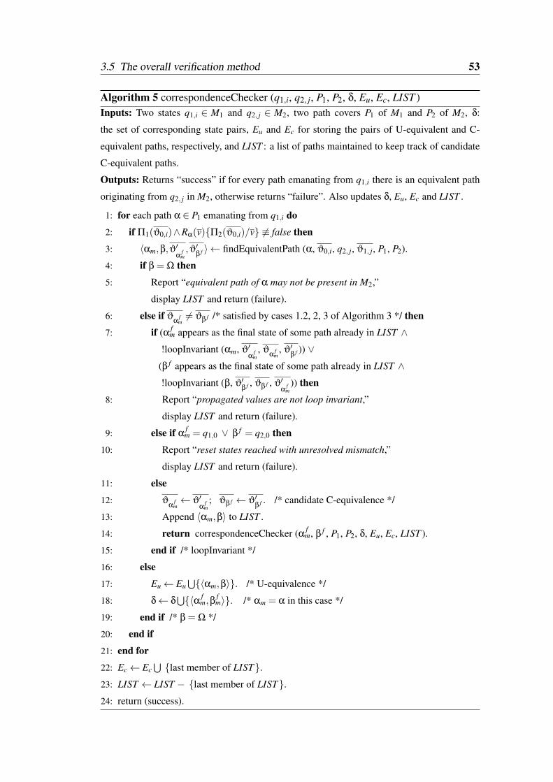
3.5 The overall verification method 53
Algorithm 5 correspondenceChecker (q1,i, q2, j, P1, P2, δ, Eu, Ec, LIST )Inputs: Two states q1,i ∈ M1 and q2, j ∈ M2, two path covers P1 of M1 and P2 of M2, δ:
the set of corresponding state pairs, Eu and Ec for storing the pairs of U-equivalent and C-
equivalent paths, respectively, and LIST : a list of paths maintained to keep track of candidate
C-equivalent paths.
Outputs: Returns “success” if for every path emanating from q1,i there is an equivalent path
originating from q2, j in M2, otherwise returns “failure”. Also updates δ, Eu, Ec and LIST .
1: for each path α ∈ P1 emanating from q1,i do
2: if Π1(ϑ0,i)∧Rα(v)Π2(ϑ0,i)/v 6≡ false then
3: 〈αm,β,ϑ′α
fm,ϑ′
β f 〉 ← findEquivalentPath (α, ϑ0,i, q2, j, ϑ1, j, P1, P2).
4: if β = Ω then
5: Report “equivalent path of α may not be present in M2,”
display LIST and return (failure).
6: else if ϑα
fm6= ϑβ f /* satisfied by cases 1.2, 2, 3 of Algorithm 3 */ then
7: if (α fm appears as the final state of some path already in LIST ∧
!loopInvariant (αm, ϑ′α
fm, ϑ
αfm, ϑ′
β f )) ∨(β f appears as the final state of some path already in LIST ∧!loopInvariant (β, ϑ′
β f , ϑβ f , ϑ′α
fm)) then
8: Report “propagated values are not loop invariant,”
display LIST and return (failure).
9: else if αfm = q1,0 ∨ β f = q2,0 then
10: Report “reset states reached with unresolved mismatch,”
display LIST and return (failure).
11: else
12: ϑα
fm← ϑ′
αfm; ϑβ f ← ϑ′
β f . /* candidate C-equivalence */
13: Append 〈αm,β〉 to LIST .
14: return correspondenceChecker (α fm, β f , P1, P2, δ, Eu, Ec, LIST ).
15: end if /* loopInvariant */
16: else
17: Eu← Eu⋃〈αm,β〉. /* U-equivalence */
18: δ← δ⋃〈α f
m,βfm〉. /* αm = α in this case */
19: end if /* β = Ω */
20: end if
21: end for
22: Ec← Ec⋃last member of LIST.
23: LIST ← LIST − last member of LIST.24: return (success).
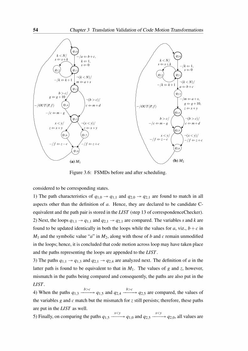
54 Chapter 3 Translation Validation of Code Motion Transformations
−/a⇐ b+ c,
¬(b > c)/
c⇐ m+d
z⇐ x+ yx < y/
z⇐ x+ y¬(x < y)/
¬(k < N)/
m⇐ a+ s−/k⇐ k+1
k⇐ 1,s⇐ 0
−/ f ⇐ z+ c
b > c/
s⇐ s+ kk < N/
−/ f ⇐ z− c
g⇐ g+10
(a) M1
q1,0
q1,1
q1,3
q1,5
q1,8
q1,4
q1,2
q1,7q1,6
−/c⇐ m−g
−/OUT (P, f )
¬(k < N)/
a⇐ b+ c−/k⇐ k+1
s⇐ 0
s⇐ s+ kk < N/
q2,0
q2,1q2,2
−/m⇐ a+ s,
q2,3
q2,4
−/k⇐ 1,
q2,5
c⇐ m+d¬(b > c)/
q2,6
b > c/−/c⇐ m−g
x < y/−/ f ⇐ z− c
¬(x < y)/−/ f ⇐ z+ c
g⇐ g+10,z⇐ x+ y
(b) M2
−/OUT (P, f )
Figure 3.6: FSMDs before and after scheduling.
considered to be corresponding states.
1) The path characteristics of q1,0 q1,1 and q2,0 q2,1 are found to match in all
aspects other than the definition of a. Hence, they are declared to be candidate C-
equivalent and the path pair is stored in the LIST (step 13 of correspondenceChecker).
2) Next, the loops q1,1 q1,1 and q2,1 q2,1 are compared. The variables s and k are
found to be updated identically in both the loops while the values for a, viz., b+ c in
M1 and the symbolic value “a” in M2, along with those of b and c remain unmodified
in the loops; hence, it is concluded that code motion across loop may have taken place
and the paths representing the loops are appended to the LIST .
3) The paths q1,1 q1,3 and q2,1 q2,4 are analyzed next. The definition of a in the
latter path is found to be equivalent to that in M1. The values of g and z, however,
mismatch in the paths being compared and consequently, the paths are also put in the
LIST .
4) When the paths q1,3b>c−−−− q1,5 and q2,4
b>c−−−− q2,5 are compared, the values of
the variables g and c match but the mismatch for z still persists; therefore, these paths
are put in the LIST as well.
5) Finally, on comparing the paths q1,5x<y−−−− q1,0 and q2,5
x<y−−−− q2,0, all values are
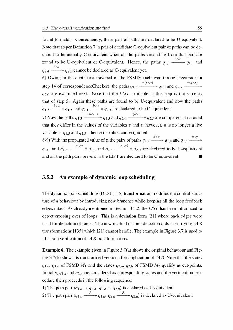
3.5 The overall verification method 55
found to match. Consequently, these pair of paths are declared to be U-equivalent.
Note that as per Definition 7, a pair of candidate C-equivalent pair of paths can be de-
clared to be actually C-equivalent when all the paths emanating from that pair are
found to be U-equivalent or C-equivalent. Hence, the paths q1,3b>c−−−− q1,5 and
q2,4b>c−−−− q2,5 cannot be declared as C-equivalent yet.
6) Owing to the depth-first traversal of the FSMDs (achieved through recursion in
step 14 of correspondenceChecker), the paths q1,5¬(x<y)−−−−−− q1,0 and q2,5
¬(x<y)−−−−−−
q2,0 are examined next. Note that the LIST available in this step is the same as
that of step 5. Again these paths are found to be U-equivalent and now the paths
q1,3b>c−−−− q1,5 and q2,4
b>c−−−− q2,5 are declared to be C-equivalent.
7) Now the paths q1,3¬(b>c)−−−−−− q1,5 and q2,4
¬(b>c)−−−−−− q2,5 are compared. It is found
that they differ in the values of the variables g and z; however, g is no longer a live
variable at q1,5 and q2,5 – hence its value can be ignored.
8-9) With the propagated value of z, the pairs of paths q1,5x<y−−−− q1,0 and q2,5
x<y−−−−
q2,0, and q1,5¬(x<y)−−−−−− q1,0 and q2,5
¬(x<y)−−−−−− q2,0 are declared to be U-equivalent
and all the path pairs present in the LIST are declared to be C-equivalent.
3.5.2 An example of dynamic loop scheduling
The dynamic loop scheduling (DLS) [135] transformation modifies the control struc-
ture of a behaviour by introducing new branches while keeping all the loop feedback
edges intact. As already mentioned in Section 3.3.2, the LIST has been introduced to
detect crossing over of loops. This is a deviation from [21] where back edges were
used for detection of loops. The new method of loop detection aids in verifying DLS
transformations [135] which [21] cannot handle. The example in Figure 3.7 is used to
illustrate verification of DLS transformations.
Example 6. The example given in Figure 3.7(a) shows the original behaviour and Fig-
ure 3.7(b) shows its transformed version after application of DLS. Note that the states
q1,a, q1,b of FSMD M1 and the states q2,a, q2,b of FSMD M2 qualify as cut-points.
Initially, q1,a and q2,a are considered as corresponding states and the verification pro-
cedure then proceeds in the following sequence.
1) The path pair 〈q1,a q1,b, q2,a q2,b〉 is declared as U-equivalent.
2) The path pair 〈q1,a¬p1−−−− q1,a, q2,a
¬p1−−−− q2,a〉 is declared as U-equivalent.
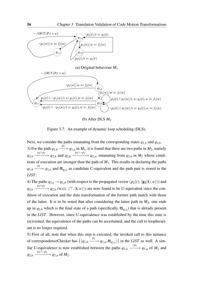
56 Chapter 3 Translation Validation of Code Motion Transformations
q1,a
q1,bq1,c
p1(w)/w⇐ f1(w)
p2(t)/t⇐ g1(t)
¬p2(t)/t⇐ g2(t)
¬p1(w)/w⇐ f2(w)
−/OUT (P, t +w)
(a) Original behaviour M1
q2,a
q2,b
p1(w)/w⇐ f1(w)
¬p2(t)∧ p1(w)/t⇐ g2(t),w⇐ f1(w)
p2(t)∧ p1(w)/t⇐ g1(t),w⇐ f1(w)
¬p1(w)/w⇐ f2(w)
q2,c
p2(t)∧¬p1(w)/t⇐ g1(t),w⇐ f2(w)
¬p2(t)∧¬p1(w)/t⇐ g2(t),w⇐ f2(w)
−/OUT (P, t +w)
(b) After DLS M2
Figure 3.7: An example of dynamic loop scheduling (DLS).
Next, we consider the paths emanating from the corresponding states q1,b and q2,b.
3) For the path q1,bp2−−− q1,a in M1, it is found that there are two paths in M2, namely
q2,bp2∧p1−−−−− q2,b and q2,b
p2∧¬p1−−−−−− q2,a, emanating from q2,b in M2 whose condi-
tions of execution are stronger than the path of M1. This results in declaring the paths
q1,bp2−−− q1,a and ϖq2,b as candidate C-equivalent and the path pair is stored in the
LIST .
4) The paths q1,a q1,b (with respect to the propagated vector 〈p2(t),〈g1(t),w〉〉) and
q2,bp2∧p1−−−−− q2,b (w.r.t. 〈>,〈t,w〉〉) are now found to be U-equivalent since the con-
dition of execution and the data transformation of the former path match with those
of the latter. It is to be noted that after considering the latter path in M2, one ends
up in q2,b which is the final state of a path (specifically, ϖq2,b) that is already present
in the LIST . However, since U-equivalence was established by the time this state is
(re)visited, the equivalence of the paths can be ascertained, and the call to loopInvari-
ant is no longer required.
5) First of all, note that when this step is executed, the invoked call to this instance
of correspondenceChecker has 〈q1,bp2−−− q1,a,ϖq2,b〉 in the LIST as well. A sim-
ilar U-equivalence is now established between the paths q1,a¬p1−−−− q1,a of M1 and
q2,bp2∧¬p1−−−−−− q2,a of M2.
3.5 The overall verification method 57
Since eventually for all paths emanating from the final state of q1,bp2−−− q1,a, a U-
equivalent path is discovered that originates from the final state of ϖq2,b , the path pair
〈q1,bp2−−− q1,a,ϖq2,b〉 is declared as actually C-equivalent, i.e. put in Ec and the LIST
is rendered empty by removing its last (and only) entry. Note that unless both the paths
from q1,a, i.e. q1,ap1−−− q1,b and q1,a
¬p1−−−− q1,a are treated, LIST is not updated –
as borne out by the fact that LIST update takes place after the loop 1 - 21 in corre-
spondenceChecker.
6) The paths q1,b¬p2−−−− q1,a and ϖq2,b are considered as candidate C-equivalent, sim-
ilar to step 3.
7-8) The path pairs 〈q1,a q1,b,q2,b¬p2∧p1−−−−−− q2,b〉 and 〈q1,a
¬p1−−−− q1,a,q2,b¬p2∧¬p1−−−−−−−
q2,a〉 are declared as U-equivalent, and 〈q1,b¬p2−−−− q1,a,ϖq2,b〉 is declared as actually
C-equivalent.
Now let us consider what would have gone wrong if back edges were used to detect
loops instead of LIST . The first two steps of the method described in [21] would have
been identical to the ones given above, and the states q1,b and q2,b would have been
declared as corresponding states. In step 3, the method in [21] would find the paths
q1,bp2−−− q1,a and ϖq2,b as candidate C-equivalent (similar to ours); however, it would
also detect q1,bp2−−− q1,a as a back edge to q1,a. While entering the loop at q1,a, the
variable t had the symbolic value “t”, but after step 3 the propagated vector computed
for q1,a would have the value g1(t) for t. Clearly, there is a mismatch in the values
for t, and therefore the method in [21] would terminate declaring the two FSMDs to
be possibly non-equivalent. It is important to note that in case of code motions across
loops, some paths will be detected to be C-equivalent while entering the loops. Hence,
whenever the entry/exit state is revisited without resolving the mismatches, the state
will definitely appear as a final state of some path in LIST , thereby leading to detection
of loops (and without having any explicit knowledge about back edges).
The bisimulation based method in [115] can handle the control structure modifi-
cations stated in the path based scheduling method [33]. In general, during path based
scheduling, two consecutive paths get concatenated into one whose condition of exe-
cution is obtained by taking the conjunction of those of its constituent paths. However,
unlike [33], DLS may introduce new branches by concatenating paths that lie within
a loop with the “exit” path of that loop (such as the branches q2,bp2∧¬p1−−−−→ q2,c and
q2,b¬p2∧¬p1−−−−−→ q2,c in Figure 3.7(b)). A primary requirement for the equivalence check-
58 Chapter 3 Translation Validation of Code Motion Transformations
ing method of [115] is that the loop exit conditions must be identical in order to find
whether two states are in a relation (a concept similar to our corresponding states);
consequently, the method of [115] results in a failure on application of DLS. For a
more sophisticated example of DLS, one may refer to [91], which both the path ex-
tension method [91, 95] and the symbolic value propagation method described in this
work can handle.
3.6 Correctness and complexity of the equivalence check-
ing procedure
3.6.1 Correctness
Theorem 3 (Partial correctness). If the verification method terminates in step 8 of the
function containmentChecker, then M1 vM2.
Proof: The proof is tantamount to ascertaining that if the verification method ter-
minates in step 8 of containmentChecker, then both hypotheses 1 and 2 of Theorem 7
are satisfied by the path covers P1 and P2 for the FSMDs M1 and M2, respectively.
The path covers P1 and P2 comprise of paths starting from and ending in cut-point(s)
without having any intermediary cut-point. The set Eu of U-equivalent paths and
Ec of C-equivalent paths are updated in steps 17 and 22, respectively, of correspon-
denceChecker. The fact that the pair of paths added to the set Eu and Ec are indeed
U-equivalent and C-equivalent, respectively, is affirmed by the function findEquiva-
lentPath.
Now, we need to prove that E = Eu⋃
Ec contains a member for each path in P1.
Suppose a path α exists in P1 that does not have a corresponding member in E. Ab-
sence of α in E indicates that the path has not been considered at all during execution
of the verification method. Since the state αs is reachable (by definition) there must
be some other path α′ that leads to it. Let us consider the following cases:
α′ ∈ E : Then E must contain some member of the form 〈α′,β′〉, where β′ ∈ P2
and either (i) α′ 'c β′ which means α would definitely have been considered in some
subsequent recursive call of correspondenceChecker, or (ii) α′ ' β′ which means the
3.6 Correctness and complexity of the equivalence checking procedure 59
end state of α′, i.e., the start state of α, must be a member of δ and α must have even-
tually been considered as given in step 4 of containmentChecker. (contradiction)
α′ 6∈ E : In such a case, one should consider the path α′′ that leads to α′. Now,
these two cases hold for α′′ as well. A repetitive application of the argument lands up
in the paths emanating from the reset state q1,0, which is a member of δ by step 2 of
containmentChecker; here steps 3 and 4 of containmentChecker ensure invocation of
correspondenceChecker with q1,i = q1,0 and step 1 of correspondenceChecker ensures
that paths from q1,0 must have been treated, thereby again leading to a contradiction.
What remains to be proved is that hypothesis 2 of Theorem 7 holds when the
verification method terminates in step 8 of containmentChecker. Suppose it does not.
Then there exist paths α ∈ P1 and β ∈ P2 such that α f = q1,0, β f = q2,0 and α'c β. It
would result in trying to extend a path beyond the reset states, and thus, the function
correspondenceChecker returns failure to containmentChecker as shown in step 10,
whereupon the latter terminates in step 5 and not in step 8. (contradiction)
Theorem 4 (Termination). The verification method always terminates.
Proof: With respect to the call graph of Figure 3.5, we prove the termination of
the modules in a bottom-up manner. The functions valuePropagation and loopIn-
variant obviously execute in finite time since the former involves comparison of two
path characteristics and two propagated vectors, whereas the latter involves compar-
ison of two propagated vectors only. The for-loop in findEquivalentPath is executed
only ‖P2‖ number of times which is finite. The outermost for-loop in the function
correspondenceChecker can be executed ‖P1‖ times which is also finite. Whenever
correspondenceChecker is invoked with the states q1,i and q2, j as arguments, there
is a possibility that the function is recursively invoked with the end states of some
path α originating from q1,i and some path β originating from q2, j. Now, it re-
mains to be shown that correspondenceChecker can invoke itself recursively only
finite number of times. Let us associate the tuple 〈n0,n1〉 ∈ N2 to each invocation
of correspondenceChecker(α fm,β
fm, . . .) (step 14), where n0 and n1 denote the number
of paths that lie ahead of αfm and β
fm in FSMD M1 and FSMD M2, respectively. (Note
that one cannot go beyond the reset states.) Also, let 〈n′0,n′1〉 < 〈n0,n1〉 if n′0 < n0
or, n′0 = n0 and n′1 < n1. Note that in the 4-tuple returned by findEquivalentPath in
step 3 of correspondenceChecker, αm and β both cannot be null paths simultaneously.
Hence, a sequence of recursive invocations of correspondenceChecker can be repre-
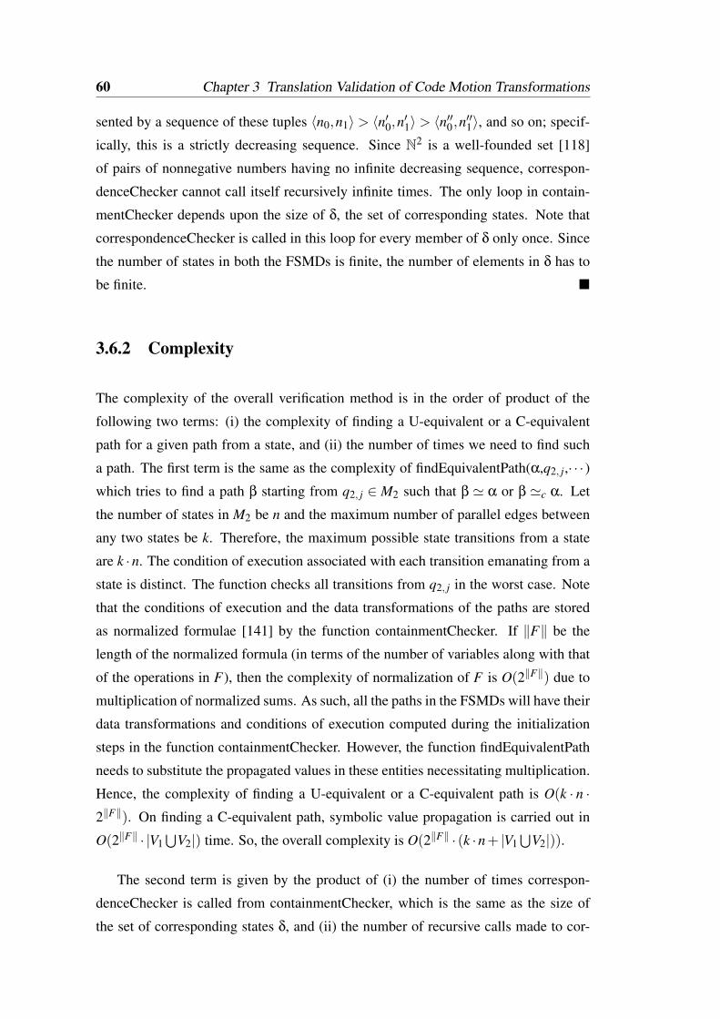
60 Chapter 3 Translation Validation of Code Motion Transformations
sented by a sequence of these tuples 〈n0,n1〉 > 〈n′0,n′1〉 > 〈n′′0,n′′1〉, and so on; specif-
ically, this is a strictly decreasing sequence. Since N2 is a well-founded set [118]
of pairs of nonnegative numbers having no infinite decreasing sequence, correspon-
denceChecker cannot call itself recursively infinite times. The only loop in contain-
mentChecker depends upon the size of δ, the set of corresponding states. Note that
correspondenceChecker is called in this loop for every member of δ only once. Since
the number of states in both the FSMDs is finite, the number of elements in δ has to
be finite.
3.6.2 Complexity
The complexity of the overall verification method is in the order of product of the
following two terms: (i) the complexity of finding a U-equivalent or a C-equivalent
path for a given path from a state, and (ii) the number of times we need to find such
a path. The first term is the same as the complexity of findEquivalentPath(α,q2, j,· · · )which tries to find a path β starting from q2, j ∈ M2 such that β ' α or β 'c α. Let
the number of states in M2 be n and the maximum number of parallel edges between
any two states be k. Therefore, the maximum possible state transitions from a state
are k ·n. The condition of execution associated with each transition emanating from a
state is distinct. The function checks all transitions from q2, j in the worst case. Note
that the conditions of execution and the data transformations of the paths are stored
as normalized formulae [141] by the function containmentChecker. If ‖F‖ be the
length of the normalized formula (in terms of the number of variables along with that
of the operations in F), then the complexity of normalization of F is O(2‖F‖) due to
multiplication of normalized sums. As such, all the paths in the FSMDs will have their
data transformations and conditions of execution computed during the initialization
steps in the function containmentChecker. However, the function findEquivalentPath
needs to substitute the propagated values in these entities necessitating multiplication.
Hence, the complexity of finding a U-equivalent or a C-equivalent path is O(k · n ·2‖F‖). On finding a C-equivalent path, symbolic value propagation is carried out in
O(2‖F‖ · |V1⋃
V2|) time. So, the overall complexity is O(2‖F‖ · (k ·n+ |V1⋃
V2|)).
The second term is given by the product of (i) the number of times correspon-
denceChecker is called from containmentChecker, which is the same as the size of
the set of corresponding states δ, and (ii) the number of recursive calls made to cor-
3.7 Experimental Results 61
respondenceChecker (in the worst case). We notice that if the number of states for
the original FSMD is n, then the number of states for the transformed FSMD is in
O(n) for both path based scheduler [33] and SPARK [64]. So, for simplicity, let the
number of states in M2 be n as well. In the worst case, all the states of M1 may be
cut-points and the number of paths in M1 is at most k · n · (n− 1)/2. In this case the
correspondenceChecker can recursively call itself as many as (n−1) times leading to
consideration of k ·(n−1)+k2 ·(n−1) ·(n−2)+ · · ·+k(n−1) ·(n−1) ·(n−2) · · ·2 ·1'k(n−1) · (n−1)(n−1) number of paths. Also, ‖δ‖ ≤ n. Therefore, the complexity of the
overall method is O((k ·n+ |V1⋃
V2|) ·2‖F‖ ·n ·k(n−1) · (n−1)(n−1)) in the worst case.
It is important to note that in [90], the authors had neglected the time complexity of
computing the path characteristics of the concatenated paths that result from path ex-
tensions. Upon considering the same, the worst case time complexity of the presented
method is found to be identical to that of [90].
3.7 Experimental Results
Table 3.1: Verification results based on our set of benchmarks
Benchmarks Original FSMD Transformed FSMD #Variable #across Maximum Time (ms)
#state #path #state #path com uncom loops mismatch PE SVP
BARCODE-1 33 54 25 56 17 0 0 3 20.1 16.2
DCT-1 16 1 8 1 41 6 0 6 6.3 3.6
DIFFEQ-1 15 3 9 3 19 3 0 4 5.0 2.6
EWF-1 34 1 26 1 40 1 0 1 4.2 3.6
LCM-1 8 11 4 8 7 2 1 4 × 2.5
IEEE754-1 55 59 44 50 32 3 4 3 × 17.7
LRU-1 33 39 32 38 19 0 2 2 × 4.0
MODN-1 8 9 8 9 10 2 0 3 5.6 2.5
PERFECT-1 6 7 4 6 8 2 2 2 × 0.9
QRS-1 53 35 24 35 25 15 3 19 × 15.9
TLC-1 13 20 7 16 13 1 0 2 9.1 4.1
The verification procedure presented in this chapter has been implemented in C
on a 2.0 GHz Intel R© CoreTM2 Duo machine and satisfactorily tested on several bench-
marks. The results are provided in Table 3.1. Some of these benchmarks, such as
BARCODE, LCM, QRS and TLC, are control intensive; some are data intensive, such
as DCT, DIFFEQ and EWF, whereas some are both control and data intensive, such as
IEEE754 and LRU. The transformed FSMD is obtained from the original one in multi-
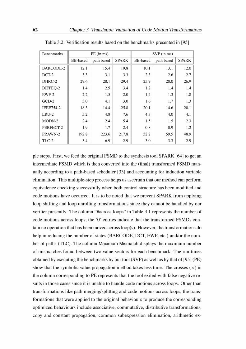
62 Chapter 3 Translation Validation of Code Motion Transformations
Table 3.2: Verification results based on the benchmarks presented in [95]
Benchmarks PE (in ms) SVP (in ms)
BB-based path based SPARK BB-based path based SPARK
BARCODE-2 12.1 15.4 19.8 10.1 13.1 12.0
DCT-2 3.3 3.1 3.3 2.3 2.6 2.7
DHRC-2 29.6 28.1 29.4 25.9 28.0 26.9
DIFFEQ-2 1.4 2.5 3.4 1.2 1.4 1.4
EWF-2 2.2 1.5 2.0 1.4 1.3 1.8
GCD-2 3.0 4.1 3.0 1.6 1.7 1.3
IEEE754-2 18.3 14.4 25.8 20.1 14.6 20.1
LRU-2 5.2 4.8 7.6 4.3 4.0 4.1
MODN-2 2.4 2.4 5.4 1.5 1.5 2.3
PERFECT-2 1.9 1.7 2.4 0.8 0.9 1.2
PRAWN-2 192.8 223.6 217.8 52.2 59.5 48.9
TLC-2 3.4 6.9 2.9 3.0 3.3 2.9
ple steps. First, we feed the original FSMD to the synthesis tool SPARK [64] to get an
intermediate FSMD which is then converted into the (final) transformed FSMD man-
ually according to a path-based scheduler [33] and accounting for induction variable
elimination. This multiple-step process helps us ascertain that our method can perform
equivalence checking successfully when both control structure has been modified and
code motions have occurred. It is to be noted that we prevent SPARK from applying
loop shifting and loop unrolling transformations since they cannot be handled by our
verifier presently. The column “#across loops” in Table 3.1 represents the number of
code motions across loops; the ‘0’ entries indicate that the transformed FSMDs con-
tain no operation that has been moved across loop(s). However, the transformations do
help in reducing the number of states (BARCODE, DCT, EWF, etc.) and/or the num-
ber of paths (TLC). The column Maximum Mismatch displays the maximum number
of mismatches found between two value-vectors for each benchmark. The run-times
obtained by executing the benchmarks by our tool (SVP) as well as by that of [95] (PE)
show that the symbolic value propagation method takes less time. The crosses (×) in
the column corresponding to PE represents that the tool exited with false negative re-
sults in those cases since it is unable to handle code motions across loops. Other than
transformations like path merging/splitting and code motions across loops, the trans-
formations that were applied to the original behaviours to produce the corresponding
optimized behaviours include associative, commutative, distributive transformations,
copy and constant propagation, common subexpression elimination, arithmetic ex-
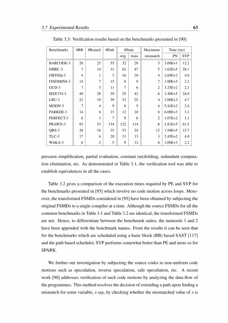
3.7 Experimental Results 63
Table 3.3: Verification results based on the benchmarks presented in [90]
Benchmarks #BB #Branch #Path #State Maximum Time (ms)
orig trans mismatch PN SVP
BARCODE-3 28 25 55 32 29 5 3.00E+3 12.2
DHRC-3 7 14 31 62 47 5 1.62E+5 28.1
DIFFEQ-3 4 1 3 16 10 4 2.69E+2 4.0
FINDMIN8-3 14 7 15 8 9 7 1.00E+5 2.3
GCD-3 7 5 11 7 6 2 3.25E+2 2.1
IEEE754-3 40 28 59 55 42 6 3.40E+5 24.0
LRU-3 22 19 39 33 25 4 3.00E+3 4.7
MODN-3 7 4 9 6 5 4 5.41E+2 2.4
PARKER-3 14 6 13 12 10 6 6.00E+3 3.1
PERFECT-3 6 3 7 9 6 2 1.07E+2 1.1
PRAWN-3 85 53 154 122 114 8 5.81E+5 61.5
QRS-3 26 16 35 53 24 12 1.94E+5 15.7
TLC-3 17 6 20 13 13 3 2.45E+2 4.0
WAKA-3 6 2 5 9 12 6 1.00E+3 2.2
pression simplification, partial evaluation, constant (un)folding, redundant computa-
tion elimination, etc. As demonstrated in Table 3.1, the verification tool was able to
establish equivalences in all the cases.
Table 3.2 gives a comparison of the execution times required by PE and SVP for
the benchmarks presented in [95] which involve no code motion across loops. More-
over, the transformed FSMDs considered in [95] have been obtained by subjecting the
original FSMDs to a single compiler at a time. Although the source FSMDs for all the
common benchmarks in Table 3.1 and Table 3.2 are identical, the transformed FSMDs
are not. Hence, to differentiate between the benchmark suites, the numerals 1 and 2
have been appended with the benchmark names. From the results it can be seen that
for the benchmarks which are scheduled using a basic block (BB) based SAST [117]
and the path based scheduler, SVP performs somewhat better than PE and more so for
SPARK.
We further our investigation by subjecting the source codes to non-uniform code
motions such as speculation, reverse speculation, safe speculation, etc. A recent
work [90] addresses verification of such code motions by analyzing the data-flow of
the programmes. This method resolves the decision of extending a path upon finding a
mismatch for some variable, x say, by checking whether the mismatched value of x is
64 Chapter 3 Translation Validation of Code Motion Transformations
used in some subsequent path or not before x is defined again. For the data-flow analy-
sis, it constructs a Kripke structure from the given behaviour, generates a CTL formula
to represent the def-use relation (for x) and employs the model checker NuSMV [38]
to find whether that formula holds in the Kripke structure or not. Depending upon the
output returned by the model checker, paths are extended accordingly. However, in the
presence of code motions across loop, the method of [90] fails due to the same reason
as that of [95], i.e., prohibition of extension of paths beyond loops. For comparing
the method of [90] with that of ours, another set of test cases have been constructed
where the original behaviours have undergone both uniform and non-uniform code
motions to produce the transformed behaviours. It is important to note that in none
of these cases code motion across loop has been applied. The time taken by our tool
and that of [90] (PN) are tabulated in Table 3.3. The method of PN takes considerable
amount of more time because it spends a large proportion of its execution time inter-
acting with NuSMV through file handling. Although a comparative analysis with the
method of [115] would have been relevant, we cannot furnish it since their tool is not
available to us.
3.8 Conclusion
In this chapter, we have presented a symbolic value propagation based equivalence
checking method which not only handles control structure modifications but also code
motions across loops apart from simpler uniform and non-uniform code motions with-
out needing any supplementary information from the synthesis tools. Specifically, the
contributions of the present chapter are as follows. (i) A new concept of symbolic
value propagation based equivalence checking has been presented for verification of
code motions across loops without compromising the capability of handling uniform
and non-uniform code motions and control structure modifications achieved in earlier
methods [90, 95]. (ii) The correctness of symbolic value propagation as a method
of equivalence checking, and the correctness and the complexity of the equivalence
checking procedure are treated formally. (iii) The computational complexity of the
presented method has been analyzed and found to be no worse than that of [90]. (iv)
Experimental results for several non-trivial benchmarks have been presented to em-
pirically establish the effectiveness of the presented method. The experimental results
demonstrate that our mechanism can verify equivalence between two behaviours even
3.8 Conclusion 65
when one of them has been subjected to successive code transformations using the
SPARK high-level synthesis tool and a path based scheduler. The method has been
tested successfully on several benchmarks, including those used in [95] and [90]. The
results show that the method performs comparably with both these methods in terms
of verification time required and outperforms them in terms of the type of transforma-
tions handled. This method does not handle transformations such as loop unrolling,
loop merging and loop shifting. Loop shifting is handled to some extent in [103, 115]
at the cost of termination; however, they cannot handle control structure transforma-
tions introduced by [135] which our method can. While there are several other tech-
niques which determine equivalence in the presence of control structure modifications,
the only techniques [80, 150] which handle code motions across loops require addi-
tional information from the synthesis tools that is difficult to obtain in general. Note
that while the method described in [150] captures infinite loops and computations that
may fail, our method is capable of handling the former but needs some improvement
to cover the latter.

Chapter 4
Deriving Bisimulation Relations fromPath Based Equivalence Checkers
4.1 Introduction
For translation validation, primarily two approaches prevail namely, bisimulation based
ones and path based ones; both have their own merits and demerits. As underlined
in Section 1.1.2, the main drawback of bisimulation based approaches is that they
require the control structures of the source and the target programs to be identical;
although this limitation is alleviated to some extent in [115] using knowledge of the
scheduling mechanism, more complex non-structure preserving transformations, such
as those applied by [135], still remain beyond their scope. On the contrary, path based
techniques [22, 90, 95] are adept in handling such non-structure preserving transfor-
mations. However, transformations such as loop shifting [44] that can be handled by
bisimulation based methods of [103, 104] still elude the path based equivalence check-
ing methods. Moreover, while the bisimulation based approaches are not guaranteed
to terminate, the path based techniques are. Considering the importance of projecting
equivalence of two behavioural specifications in terms of a bisimulation relation be-
tween them, in this chapter we evolve a mechanism of deriving one from the output
of a path based equivalence checker.
We define the notion of simulation and bisimulation relations in the context of the
FSMD model in Section 4.2. We then show in Sections 4.3 and 4.4 that a bisimulation
67
68 Chapter 4 Deriving Bisimulation Relations
relation can be constructed whenever two FSMDs are found to be equivalent by both a
path extension based and a symbolic value propagation based equivalence checker. It
is to be noted that none of the bisimulation relation based approaches has been shown
to tackle code motion across loops; therefore, the present work demonstrates, for the
first time, that a bisimulation relation exists even under such a context. The chapter is
concluded in Section 4.5.
4.2 The simulation and the bisimulation relations be-
tween FSMD models
Let us consider the FSMD model 〈Q,q0, I,V,O,τ : Q× 2S → Q, h : Q× 2S → U〉,with the notations having their usual meanings as mentioned in Section 3.2. Let v
denote a vector (an ordered tuple) of variables of I and V assuming values from the
domain Dv = Λv∈I∪V Dv, where Dv is the domain of the variable v and Λ represents
the Cartesian product of sets. Let q(v), q ∈Q, denote the set of values assumed by the
variables in the state q. Each element of q(v) is called a data state at q and is denoted
as σq. Let Σ =⋃
q∈Qσq be the set of all the data states.
An FSMD can be represented in a natural way as a digraph with the control states
as the vertices and the labeled edges capturing the transition function τ and the update
function h. Specifically, if there are two control states qi and q j such that τ(qi,c(v)) =
q j and h(qi,c(v)) is represented as v⇐ f (v), then there is an edge from qi to q j with
label c(v)/v⇐ f (v) in the digraph representation of the FSMD. A transition which
updates a storage variable with an input is called an input transition. A transition
which updates an output variable is called an output transition. A control state along
with a data state together constitute a configuration as defined below.
Definition 8 (Configuration). Given an FSMD M = 〈Q,q0, I,V,O,τ,h〉, we define a
configuration to be a pair 〈q,σ〉, where q ∈ Q and σ ∈ q(v).
Definition 9 (Execution Sequence). For a given FSMD M = 〈Q,q0, I,V,O,τ,h〉, an ex-
ecution sequence η is a sequence of configurations of the form 〈〈qi0,σi0〉,〈qi1,σi1〉, . . . ,〈qin,σin〉〉, such that ∀ j,0 ≤ j ≤ n,σi j ∈ qi j(v),τ(qi j ,c(σi j)) = qi j+1 , where c(σi j) is
true and h(qi j ,c(σi j)) ∈U defines the update operation by which the data state σi j+1
is obtained from σi j .
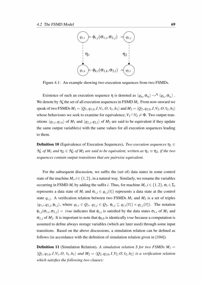
4.2 The FSMD Model 69
q1,i
q1,k
η1
q2, j
q2,l
η2
φi, j(σ1,i,σ2, j)
φk,l(σ1,k,σ2,l)
Figure 4.1: An example showing two execution sequences from two FSMDs.
Existence of such an execution sequence η is denoted as 〈qi0 ,σi0〉;η 〈qin,σin〉 .
We denote by Ni the set of all execution sequences in FSMD Mi. From now onward we
speak of two FSMDs M1 = 〈Q1,q1,0, I,V1,O, τ1,h1〉 and M2 = 〈Q2,q2,0, I,V2,O,τ2,h2〉whose behaviours we seek to examine for equivalence; V1∩V2 6= Φ. Two output tran-
sitions 〈q1,i,q1,k〉 of M1 and 〈q2, j,q2,l〉 of M2 are said to be equivalent if they update
the same output variable(s) with the same values for all execution sequences leading
to them.
Definition 10 (Equivalence of Execution Sequences). Two execution sequences η1 ∈N1 of M1 and η2 ∈N2 of M2 are said to be equivalent, written as η1 ≡ η2, if the two
sequences contain output transitions that are pairwise equivalent.
For the subsequent discussion, we suffix the (set of) data states in some control
state of the machine Mi, i∈ 1,2, in a natural way. Similarly, we rename the variables
occurring in FSMD Mi by adding the suffix i. Thus, for machine Mi, i∈ 1,2, σi ∈ Σi
represents a data state of Mi and σi, j ∈ qi, j(vi) represents a data state at the control
state qi, j. A verification relation between two FSMDs M1 and M2 is a set of triples
〈q1,i,q2, j,φi, j〉, where q1,i ∈ Q1, q2, j ∈ Q2, φi, j ⊆ q1,i(v1)× q2, j(v2). The notation
φi, j(σ1,i,σ2, j) = true indicates that φi, j is satisfied by the data states σ1,i of M1 and
σ2, j of M2. It is important to note that φ0,0 is identically true because a computation is
assumed to define always storage variables (which are later used) through some input
transitions. Based on the above discussions, a simulation relation can be defined as
follows (in accordance with the definition of simulation relation given in [104]).
Definition 11 (Simulation Relation). A simulation relation S for two FSMDs M1 =
〈Q1,q1,0, I,V1,O, τ1,h1〉 and M2 = 〈Q2,q2,0, I,V2,O,τ2,h2〉 is a verification relation
which satisfies the following two clauses:

70 Chapter 4 Deriving Bisimulation Relations
1. S(q1,0,q2,0, true), and
2. ∀q1,i,q1,k ∈ Q1,σ1,i ∈ q1,i(v),σ1,k ∈ q1,k(v), η1 ∈N1,q2, j ∈ Q2,σ2, j ∈ q2, j(v)[〈q1,i,σ1,i〉;η1 〈q1,k,σ1,k〉 ∧ φi, j(σ1,i,σ2, j) ∧ S(q1,i,q2, j,φi, j)⇒∃q2,l ∈ Q2,σ2,l ∈ q2,l(v),η2 ∈N2〈q2, j,σ2, j〉;η2 〈q2,l,σ2,l〉 ∧ η1 ≡ η2 ∧ φk,l(σ1,k,σ2,l) ∧ S(q1,k,q2,l,φk,l)
].
Intuitively, the two clauses mentioned above state that: (i) the reset state of FSMD
M1 must be related to the reset state of FSMD M2 for all data states, and (ii) if two
states of M1 and M2 with their respective data states are related and M1 can proceed
along an execution sequence, η1 say, then M2 must also be able to proceed along an
execution sequence, η2 say, such that η1 ≡ η2 and the end states of the two execution
sequences must also be related. Figure 4.1 depicts the second clause of the defini-
tion diagrammatically. We now define a bisimulation relation using the definition of
simulation relation.
Definition 12 (Bisimulation Relation). A verification relation B for two FSMDs M1
and M2 is a bisimulation relation between them iff B is a simulation relation for M1,M2
and B−1 = (q2, j,q1,i,φ) | B(q1,i,q2, j,φ) is a simulation relation for M2,M1.
4.3 Deriving simulation relation from the output of a
path extension based equivalence checker
In light of the definitions given in the previous section, let us revisit some of the earlier
notions which we have come across in Section 3.2. A path α is characterized by an or-
dered pair 〈Rα,rα〉, where Rα is the condition of execution of α satisfying the property
that ∀σαs ∈ Σ, Rα(σαs) implies that the path α is executed if control reaches the state
αs; the second member rα = 〈sα,θα〉, where sα is the functional transformation of the
path α, i.e., σα f = sα(σαs) and θα represents the output list of data values of some
variables produced along the path α. The relation of corresponding states is denoted
as δ⊆ Q1×Q2. Based on the above discussion, we now define a verification relation
between two FSMDs.
Definition 13 (Type-I Verification Relation). A type-I verification relation V for two
FSMDs M1 = 〈Q1,q1,0, I,V1,O,τ1,h1〉 and M2 = 〈Q2,q2,0, I,V2,O,τ2,h2〉 is a verifi-
cation relation which satisfies the following two clauses:
4.3 From path extension based equivalence checker 71
1. V (q1,0,q2,0, true), and
2. ∀q1,k ∈ Q1, q2,l ∈ Q2[
V (q1,k,q2,l,φk,l)⇔∃q1,i ∈ Q1(q1,i q1,k ∈ P1) ∧∀q1,i ∈ Q1
q1,i q1,k = α, say, ∈ P1⇒
∃q2, j ∈ Q2(
q2, j q2,l = β, say, ∈ P2 ∧ α' β ∧ V (q1,i,q2, j,φi, j)) ]
.
Theorem 5. The verification relation V for two FSMDs M1,M2 is a simulation rela-
tion for M1,M2, i.e., ∀〈q1,i,q2, j,φi, j〉,〈q1,i,q2, j,φi, j〉 ∈ V ⇒ 〈q1,i,q2, j,φi, j〉 ∈ S
Proof: For the pair of reset states, 〈q1,0,q2,0, true〉 is in V and also in S by the
respective first clauses in Definition 13 and Definition 11. For 〈q1,k,q2,l,φk,l〉 ∈ V ,
where q1,k 6= q1,0 and q2,l 6= q2,0, by application of clause 2 in Definition 13 m times,
m ≥ 1, we may conclude that there exists a sequence of paths α1,α2, . . . ,αm, where
αh ∈ P1,1≤ h≤ m, and another sequence of paths β1,β2, . . . ,βm, where βh ∈ P2,1≤h ≤ m, such that αs
1 = q1,0,αfm = q1,k,β
s1 = q2,0,β
fm = q2,l and αh ' βh,1 ≤ h ≤
m; also the corresponding sequence of configurations 〈q1,0,σ1,0〉α1−−− 〈q1,i1,σ1,i1〉
α2−−− · · ·αm−−− 〈q1,im = q1,k,σ1,im = σ1,k〉 and 〈q2,0,σ2,0〉
β1−−− 〈q2, j1,σ2, j1〉β2−−−
· · ·βm−−− 〈q2, jm = q2,l,σ2, jm =σ2,l〉 satisfy the property that 〈q1,ih,q2, jh,φih, jh〉 ∈V ,1≤
h≤m. We shall prove that 〈q1,ih,q2, jh,φih, jh〉 ∈ S,1≤ h≤m, holds by induction on h.
Basis case (h = 1): In this case, there must exist a single path q1,0 q1,k = α1 in
P1 and a path q2,0 q2,l = β1 in P2 such that α1 ' β1; additionally, we also have
σ1,k = sα1(σ1,0) and σ2,l = sβ1(σ2,0). So, in clause 2 of Definition 11, let q1,i =
q1,0,σ1,i = σ1,0,σ1,k = sα1(σ1,0) so that σ1,k ∈ q1,k(v),η1 =α1,q2, j = q2,0,σ2, j = σ2,0.
We notice that the antecedents of clause 2 in Definition 11 hold; specifically, the an-
tecedent 〈q1,0,σ1,0〉 ;η1 〈q1,k,σ1,k〉 holds by the right hand side (rhs) of clause 2
in Definition 13; the antecedent φ0,0(σ1,0,σ2,0) holds since φ0,0 is identically true;
〈q1,0,q2,0,φ0,0〉 ∈ S by clause 1 in Definition 11. Hence, the consequents of clause 2
in Definition 11 hold with σ2,l = sβ1(σ2,0),η2 = β1; so from the fourth consequent,
we have 〈q1,k,q2,l,φk,l〉 ∈ S.
Induction hypothesis: Let 〈q1,k,q2,l,φk,l〉 ∈ S hold whenever the states q1,k in Q1 and
q2,l in Q2 are reachable from q1,0 and q2,0, respectively, through sequences of length
n of pairwise equivalent paths from P1 and P2.
Induction step: Let the state q1,k be reachable from q1,0 through the sequence q1,0α1−−−
q1,i1α2−−− · · ·
αn−−− q1,inαn+1−−−− q1,k in M1 and the state q2,l be reachable from q2,0
through the sequence q2,0β1−−− q2, j1
β2−−− · · ·βn−−− q2, jn
βn+1−−−− q2,l in M2 such
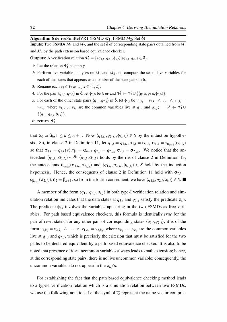
72 Chapter 4 Deriving Bisimulation Relations
Algorithm 6 deriveSimRelVR1 (FSMD M1, FSMD M2, Set δ)Inputs: Two FSMDs M1 and M2, and the set δ of corresponding state pairs obtained from M1
and M2 by the path extension based equivalence checker.
Outputs: A verification relation V1 = 〈q1,k,q2,l,φk,l〉|〈q1,k,q2,l〉 ∈ δ.
1: Let the relation V1 be empty.
2: Perform live variable analyses on M1 and M2 and compute the set of live variables for
each of the states that appears as a member of the state pairs in δ.
3: Rename each v j ∈Vi as vi, j, i ∈ 1,2.4: For the pair 〈q1,0,q2,0〉 in δ, let φ0,0 be true and V1← V1∪〈q1,0,q2,0,φ0,0〉.5: For each of the other state pairs 〈q1,i,q2, j〉 in δ, let φi, j be v1,k1 = v2,k1 ∧ . . . ∧ v1,kn =
v2,kn , where vk1 , . . . ,vkn are the common variables live at q1,i and q2, j; V1 ← V1 ∪〈q1,i,q2, j,φi, j〉.
6: return V1.
that αh ' βh,1 ≤ h ≤ n+ 1. Now 〈q1,in ,q2, jn,φin, jn〉 ∈ S by the induction hypothe-
sis. So, in clause 2 in Definition 11, let q1,i = q1,in,σ1,i = σ1,in,σ1,k = sαn+1(σ1,in)
so that σ1,k = q1,k(v),η1 = αn+1,q2, j = q2, jn,σ2, j = σ2, jn . We notice that the an-
tecedent 〈q1,in,σ1,in〉;η1 〈q1,k,σ1,k〉 holds by the rhs of clause 2 in Definition 13;
the antecedents φin, jn(σ1,in,σ2, jn) and 〈q1,in ,q2, jn,φin, jn〉 ∈ S hold by the induction
hypothesis. Hence, the consequents of clause 2 in Definition 11 hold with σ2,l =
sβn+1(σ2, jn),η2 = βn+1; so from the fourth consequent, we have 〈q1,k,q2,l,φk,l〉 ∈ S.
A member of the form 〈q1,i,q2, j,φi, j〉 in both type-I verification relation and sim-
ulation relation indicates that the data states at q1,i and q2, j satisfy the predicate φi, j.
The predicate φi, j involves the variables appearing in the two FSMDs as free vari-
ables. For path based equivalence checkers, this formula is identically true for the
pair of reset states; for any other pair of corresponding states 〈q1,i,q2, j〉, it is of the
form v1,k1 = v2,k1 ∧ . . . ∧ v1,kn = v2,kn , where vk1, . . . ,vkn are the common variables
live at q1,i and q2, j, which is precisely the criterion that must be satisfied for the two
paths to be declared equivalent by a path based equivalence checker. It is also to be
noted that presence of live uncommon variables always leads to path extension; hence,
at the corresponding state pairs, there is no live uncommon variable; consequently, the
uncommon variables do not appear in the φi, j’s.
For establishing the fact that the path based equivalence checking method leads
to a type-I verification relation which is a simulation relation between two FSMDs,
we use the following notation. Let the symbol vc represent the name vector compris-
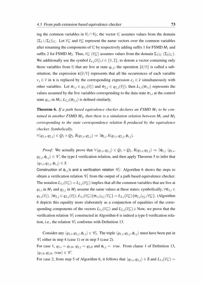
4.3 From path extension based equivalence checker 73
ing the common variables in V1 ∩V2; the vector vc assumes values from the domain
(Σ1 ∪Σ2)|vc . Let v1c and v2c represent the name vectors over the common variables
after renaming the components of vc by respectively adding suffix 1 for FSMD M1 and
suffix 2 for FSMD M2. Thus, v1c (v2c) assumes values from the domain Σ1|vc (Σ2|vc).
We additionally use the symbol Li, j(vi), i ∈ 1,2, to denote a vector containing only
those variables from vi that are live at state qi, j; the operation e/v is called a sub-
stitution; the expression κe/v represents that all the occurrences of each variable
v j ∈ v in κ is replaced by the corresponding expression e j ∈ e simultaneously with
other variables. Let σ1,i ∈ q1,i(v1) and σ2, j ∈ q2, j(v2); then L1,i(σ1,i) represents the
values assumed by the live variables corresponding to the data state σ1,i at the control
state q1,i in M1; L2, j(σ2, j) is defined similarly.
Theorem 6. If a path based equivalence checker declares an FSMD M1 to be con-
tained in another FSMD M2, then there is a simulation relation between M1 and M2
corresponding to the state correspondence relation δ produced by the equivalence
checker. Symbolically,
∀〈q1,i,q2, j〉 ∈ Q1×Q2, δ(q1,i,q2, j)⇒∃φi, j S(q1,i,q2, j,φi, j).
Proof: We actually prove that ∀〈q1,i,q2, j〉 ∈ Q1×Q2, δ(q1,i,q2, j)⇒ ∃φi, j 〈q1,i,
q2, j,φi, j〉 ∈ V , the type-I verification relation, and then apply Theorem 5 to infer that
〈q1,i,q2, j,φi, j〉 ∈ S.
Construction of φi, j ’s and a verification relation V1: Algorithm 6 shows the steps to
obtain a verification relation V1 from the output of a path based equivalence checker.
The notation L1,i(v1c) = L2, j(v2c) implies that all the common variables that are live at
q1,i in M1 and q2, j in M2 assume the same values at these states; symbolically, ∀σ1,i ∈q1,i(v1), ∃σ2, j ∈ q2, j(v2), L1,i(v1c)σ1,i|v1c/v1c= L2, j(v2c)σ2, j|v2c/v2c. (Algorithm
6 depicts this equality more elaborately as a conjunction of equalities of the corre-
sponding components of the vectors L1,i(v1c) and L2, j(v2c).) Now, we prove that the
verification relation V1 constructed in Algorithm 6 is indeed a type-I verification rela-
tion, i.e., the relation V1 conforms with Definition 13.
Consider any 〈q1,i,q2, j,φi, j〉 ∈V1. The triple 〈q1,i,q2, j,φi, j〉 must have been put in
V1 either in step 4 (case 1) or in step 5 (case 2).
For case 1, q1,i = q1,0, q2, j = q2,0 and φi, j = true. From clause 1 of Definition 13,
〈q1,0,q2,0, true〉 ∈ V .
For case 2, from step 5 of Algorithm 6, it follows that 〈q1,i,q2, j〉 ∈ δ and L1,i(v1c) =
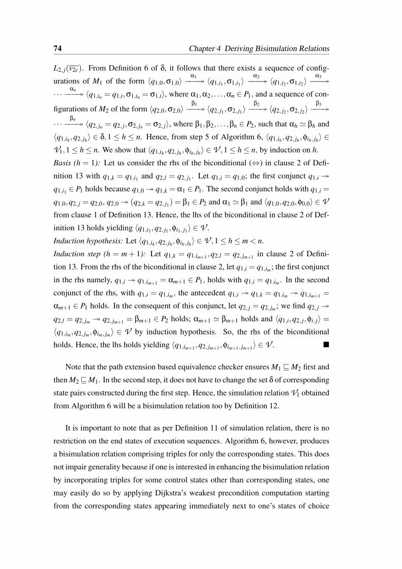
74 Chapter 4 Deriving Bisimulation Relations
L2, j(v2c). From Definition 6 of δ, it follows that there exists a sequence of config-
urations of M1 of the form 〈q1,0,σ1,0〉α1−−− 〈q1,i1 ,σ1,i1〉
α2−−− 〈q1,i2,σ1,i2〉α3−−−
· · ·αn−−− 〈q1,in = q1,i,σ1,in = σ1,i〉, where α1,α2, . . . ,αn ∈ P1, and a sequence of con-
figurations of M2 of the form 〈q2,0,σ2,0〉β1−−− 〈q2, j1,σ2, j1〉
β2−−− 〈q2, j2,σ2, j2〉β3−−−
· · ·βn−−− 〈q2, jn = q2, j,σ2, jn = σ2, j〉, where β1,β2, . . . ,βn ∈ P2, such that αh ' βh and
〈q1,ih,q2, jh〉 ∈ δ,1 ≤ h ≤ n. Hence, from step 5 of Algorithm 6, 〈q1,ih ,q2, jh,φih, jh〉 ∈V1,1≤ h≤ n. We show that 〈q1,ih ,q2, jh,φih, jh〉 ∈ V ,1≤ h≤ n, by induction on h.
Basis (h = 1): Let us consider the rhs of the biconditional (⇔) in clause 2 of Defi-
nition 13 with q1,k = q1,i1 and q2,l = q2, j1 . Let q1,i = q1,0; the first conjunct q1,i
q1,i1 ∈ P1 holds because q1,0 q1,k = α1 ∈ P1. The second conjunct holds with q1,i =
q1,0,q2, j = q2,0, q2,0 (q2,k = q2, j1) = β1 ∈ P2 and α1 ' β1 and 〈q1,0,q2,0,φ0,0〉 ∈ Vfrom clause 1 of Definition 13. Hence, the lhs of the biconditional in clause 2 of Def-
inition 13 holds yielding 〈q1,i1,q2, j1,φi1, j1〉 ∈ V .
Induction hypothesis: Let 〈q1,ih ,q2, jh,φih, jh〉 ∈ V ,1≤ h≤ m < n.
Induction step (h = m+ 1): Let q1,k = q1,im+1,q2,l = q2, jm+1 in clause 2 of Defini-
tion 13. From the rhs of the biconditional in clause 2, let q1,i = q1,im; the first conjunct
in the rhs namely, q1,i q1,im+1 = αm+1 ∈ P1, holds with q1,i = q1,im . In the second
conjunct of the rhs, with q1,i = q1,im, the antecedent q1,i q1,k = q1,im q1,im+1 =
αm+1 ∈ P1 holds. In the consequent of this conjunct, let q2, j = q2, jm; we find q2, j
q2,l = q2, jm q2, jm+1 = βm+1 ∈ P2 holds; αm+1 ' βm+1 holds and 〈q1,i,q2, j,φi, j〉 =〈q1,im,q2, jm,φim, jm〉 ∈ V by induction hypothesis. So, the rhs of the biconditional
holds. Hence, the lhs holds yielding 〈q1,im+1,q2, jm+1,φim+1, jm+1〉 ∈ V .
Note that the path extension based equivalence checker ensures M1 vM2 first and
then M2vM1. In the second step, it does not have to change the set δ of corresponding
state pairs constructed during the first step. Hence, the simulation relation V1 obtained
from Algorithm 6 will be a bisimulation relation too by Definition 12.
It is important to note that as per Definition 11 of simulation relation, there is no
restriction on the end states of execution sequences. Algorithm 6, however, produces
a bisimulation relation comprising triples for only the corresponding states. This does
not impair generality because if one is interested in enhancing the bisimulation relation
by incorporating triples for some control states other than corresponding states, one
may easily do so by applying Dijkstra’s weakest precondition computation starting
from the corresponding states appearing immediately next to one’s states of choice
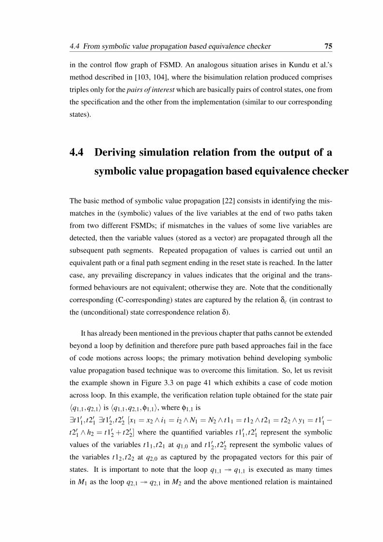
4.4 From symbolic value propagation based equivalence checker 75
in the control flow graph of FSMD. An analogous situation arises in Kundu et al.’s
method described in [103, 104], where the bisimulation relation produced comprises
triples only for the pairs of interest which are basically pairs of control states, one from
the specification and the other from the implementation (similar to our corresponding
states).
4.4 Deriving simulation relation from the output of a
symbolic value propagation based equivalence checker
The basic method of symbolic value propagation [22] consists in identifying the mis-
matches in the (symbolic) values of the live variables at the end of two paths taken
from two different FSMDs; if mismatches in the values of some live variables are
detected, then the variable values (stored as a vector) are propagated through all the
subsequent path segments. Repeated propagation of values is carried out until an
equivalent path or a final path segment ending in the reset state is reached. In the latter
case, any prevailing discrepancy in values indicates that the original and the trans-
formed behaviours are not equivalent; otherwise they are. Note that the conditionally
corresponding (C-corresponding) states are captured by the relation δc (in contrast to
the (unconditional) state correspondence relation δ).
It has already been mentioned in the previous chapter that paths cannot be extended
beyond a loop by definition and therefore pure path based approaches fail in the face
of code motions across loops; the primary motivation behind developing symbolic
value propagation based technique was to overcome this limitation. So, let us revisit
the example shown in Figure 3.3 on page 41 which exhibits a case of code motion
across loop. In this example, the verification relation tuple obtained for the state pair
〈q1,1,q2,1〉 is 〈q1,1,q2,1,φ1,1〉, where φ1,1 is
∃t1′1, t2′1 ∃t1′2, t2′2 [x1 = x2 ∧ i1 = i2 ∧N1 = N2 ∧ t11 = t12 ∧ t21 = t22 ∧ y1 = t1′1−t2′1 ∧ h2 = t1′2 + t2′2] where the quantified variables t1′1, t2
′1 represent the symbolic
values of the variables t11, t21 at q1,0 and t1′2, t2′2 represent the symbolic values of
the variables t12, t22 at q2,0 as captured by the propagated vectors for this pair of
states. It is important to note that the loop q1,1 q1,1 is executed as many times
in M1 as the loop q2,1 q2,1 in M2 and the above mentioned relation is maintained
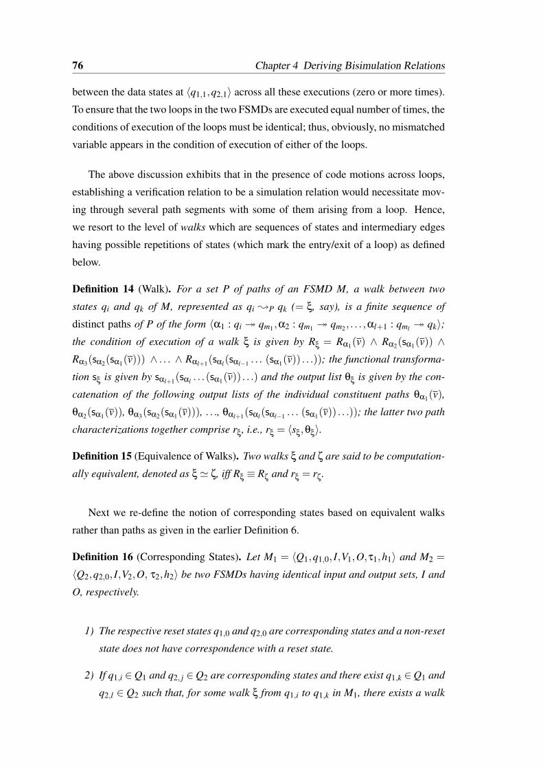
76 Chapter 4 Deriving Bisimulation Relations
between the data states at 〈q1,1,q2,1〉 across all these executions (zero or more times).
To ensure that the two loops in the two FSMDs are executed equal number of times, the
conditions of execution of the loops must be identical; thus, obviously, no mismatched
variable appears in the condition of execution of either of the loops.
The above discussion exhibits that in the presence of code motions across loops,
establishing a verification relation to be a simulation relation would necessitate mov-
ing through several path segments with some of them arising from a loop. Hence,
we resort to the level of walks which are sequences of states and intermediary edges
having possible repetitions of states (which mark the entry/exit of a loop) as defined
below.
Definition 14 (Walk). For a set P of paths of an FSMD M, a walk between two
states qi and qk of M, represented as qi ;P qk (= ξ, say), is a finite sequence of
distinct paths of P of the form 〈α1 : qi qm1 ,α2 : qm1 qm2, . . . ,αl+1 : qml qk〉;the condition of execution of a walk ξ is given by Rξ = Rα1(v) ∧ Rα2(sα1(v)) ∧Rα3(sα2(sα1(v))) ∧ . . . ∧ Rαl+1(sαl(sαl−1 . . . (sα1(v)) . . .)); the functional transforma-
tion sξ is given by sαl+1(sαl . . .(sα1(v)) . . .) and the output list θξ is given by the con-
catenation of the following output lists of the individual constituent paths θα1(v),
θα2(sα1(v)), θα3(sα2(sα1(v))), . . ., θαl+1(sαl(sαl−1 . . . (sα1(v)) . . .)); the latter two path
characterizations together comprise rξ, i.e., rξ = 〈sξ,θξ〉.
Definition 15 (Equivalence of Walks). Two walks ξ and ζ are said to be computation-
ally equivalent, denoted as ξ' ζ, iff Rξ ≡ Rζ and rξ = rζ.
Next we re-define the notion of corresponding states based on equivalent walks
rather than paths as given in the earlier Definition 6.
Definition 16 (Corresponding States). Let M1 = 〈Q1,q1,0, I,V1,O,τ1,h1〉 and M2 =
〈Q2,q2,0, I,V2,O, τ2,h2〉 be two FSMDs having identical input and output sets, I and
O, respectively.
1) The respective reset states q1,0 and q2,0 are corresponding states and a non-reset
state does not have correspondence with a reset state.
2) If q1,i ∈Q1 and q2, j ∈Q2 are corresponding states and there exist q1,k ∈Q1 and
q2,l ∈ Q2 such that, for some walk ξ from q1,i to q1,k in M1, there exists a walk
4.4 From symbolic value propagation based equivalence checker 77
−/x⇐ 0,y⇐ 20
q2, j
q2,n
q2,l′
¬(x < N)/y⇐ y+2
(b) M2
q2,l
−/z⇐ x+ y
x < N/x⇐ x+1
¬(x < N)/z⇐ x+ y
−/x⇐ 0,y⇐ 18
q1,k
(a) M1
x < N/x⇐ x+1,y⇐ y+4 q1,m
q1,i
Figure 4.2: An example of non-equivalent programs.
ζ from q2, j to q2,l in M2 such that ξ ' ζ, then q1,k and q2,l are corresponding
states (note that q1,k and q2,l must both be either reset states or non-reset states).
In addition to the set of corresponding states δ, we also maintain the set of cor-
responding loop states to store pairs of the entry/exit states of those loops which are
reached with loop invariant propagated vectors, such as 〈q1,1,q2,1〉 in Figure 3.3; let
the set of such corresponding loop states be denoted as δ.
Let us now briefly revisit the path extension based equivalence checking method
as mentioned in Section 4.3. In this method, we had a path cover P of an FSMD
M such that every computation of M could be looked upon as a concatenation of
paths (possibly, with repetitions) from the path cover P. Note that in the present
scenario, we cannot define a similar notion of walk cover since a walk cover may have
to accommodate infinite number of walks to capture arbitrary number of executions
of loops. The walks that are considered by our symbolic value propagation based
equivalence checker does not allow for repetition of paths (as given in Definition 14);
if a walk contains any subsequence (of paths) with identical start and end states, then
that subsequence represents a loop. Let ξ be a walk in FSMD M of the form ξpξlξs
with a prefix sequence ξp (“p” for prefix), a sequence ξl (“l” for loop) with identical
start and end state and a suffix sequence ξs (“s” for suffix); we call a walk such as
ξ as a single loop walk (SLW). Walks containing SLWs where the loop segments are
entered with mismatches in variables can have equivalent walks in the other FSMD
provided the mismatches do not change over the loop iterations as illustrated below.
In Figure 4.2(a), let the path q1,i q1,m be ξp, the loop q1,m q1,m be ξl and
the path q1,m q1,k be ξs. Similarly, in Figure 4.2(b), let the path q2, j q2,n be ζp,
78 Chapter 4 Deriving Bisimulation Relations
the loop q2,n q2,n be ζl and the path q2,n q2,l be ζs. It is important to note that
the SLWs ξpξlξs and ζpζlζs are equivalent having identical condition of execution
Rξ ≡ Rζ ≡ (0 < N)∧¬(1 < N) and identical data transformations sξ = sζ = x⇐1,y⇐ 22,z⇐ 23 for N = 1. However, for any integer value of N other than 1,
the computations of the two programs will be different. For example, for N = 5, the
source program will assign the value 43 to the variable z, whereas, the transformed
program will assign the value 27 to z.
Note that the symbolic value propagation based equivalence checker identifies two
such SLWs, ξ of M1 and ζ of M2, as equivalent (or more specifically, starting with the
corresponding states 〈ξs,ζs〉, identifies 〈ξ f ,ζ f 〉 as corresponding states) if there are
propagation vectors γ1 and γ2, say, at ξfp and ζ
fp respectively depicting mismatches
over ξp and ζp which satisfy the following three conditions:
(i) γ1 and γ2 disappear (i.e., all mismatches are compensated for) over the segments
ξfp(= ξs
s) to ξfs and ζ
fp(= ζs
s) to ζfs ,
(ii) γ1 and γ2 remain invariant over the loops ξl and ζl , respectively, and
(iii) the conditions of execution ξl and ζl are identical (involving no variable which
has mismatch as per γ1 and γ2).
Conditions (i) and (ii) indicate that code motions may have taken place from ξp
to ξs across the loop ξl , or from ζp to ζs across the loop ζl or both. Condition (iii)
implies that the loops ξl and ζl are executed identical number of times. Only under
these conditions, ξ ' ζ ⇒ ξp(ξl)mξs ' ζp(ζl)
mζs, ∀m ≥ 0, where m represents the
number of times the loops ξl and ζl are iterated. Stated in words, the loop invariance
of the propagated vectors at the entry/exit states of the loop preserves equivalence
of SLWs under pumping of the loops equal number of times. The following lemma
supports the observation.
Lemma 1 (Pumping Lemma for SLWs). Let ξ = ξpξlξs be an SLW of M1 and ζ =
ζpζlζs be an SLW of M2 such that 〈ξs,ζs〉 ∈ δ; let γ1 and γ2 be the propagation vectors
over ξp and ζp, respectively. If γ1 and γ2 are loop invariant over ξl and ζl , respectively,
then ξ' ζ ⇒ ξp(ξl)mξs ' ζp(ζl)
mζs, ∀m≥ 0.
Proof: The constraint 〈ξs,ζs〉 ∈ δ implies that all the (common) live variables must
have identical values at ξs in M1 and ζs in M2. Let v be a variable whose definitions
mismatch at ξfp(= ξs
l ) and ζfp(= ζs
l ). Since the propagated vectors γ1 and γ2 are loop
4.4 From symbolic value propagation based equivalence checker 79
invariant, the variables which have the mismatches at ξsl and ζs
l as well as those which
appear in their symbolic expression values are not assigned any new values and the
other variables are transformed identically. In short, therefore, sξl= sζl
. Also, the con-
ditions of execution of the loops, Rξland Rζl
, are equivalent and do not involve any
variables which have mismatches at ξsl and ζs
l . Under this scenario, the loops ξl and
ζl will iterate identical number of times, smξl(sξp(v1)) and sm
ζl(sζp(v2)) will have the
same mismatch and Rξl(sm
ξl(sξp(v1))) ≡ Rζl
(smζl(sζp(v2))),∀m ≥ 0. It further implies
that mismatched variables, such as v, must not have been output in ξl and ζl , and also
not used in determining the value of any other variable. Finally, the antecedent ξ' ζ
implies that the mismatch in definitions must have disappeared at 〈ξ f ,ζ f 〉; hence,
Rξp(v1)∧Rξl(sξp(v1))∧Rξs(sξl
(sξp(v1)))≡ Rζp(v2)∧Rζl(sζp(v2))∧Rζs(sζl
(sζp(v2)))
and sξs(sξl(sξp(v1))) = sζs(sζl
(sζp(v2))). Therefore, from Rξl≡Rζl
and sξl= sζl
, it fol-
lows that Rξp(v1)∧Rξl(sξp(v1))∧Rξl
(sξl(sξp(v1)))∧Rξs(sξl
(sξl(sξp(v1))))≡ Rζp(v2)∧
Rζl(sζp(v2))∧Rζl
(sζl(sζp(v2)))∧Rζs(sζl
(sζl(sζp(v2)))) and sξs(sξl
(sξl(sξp(v1)))) =
sζs(sζl(sζl
(sζp(v2)))); repetition of the argument m−1 times gives Rξp(v1)∧Rξl(sm−1
ξl(
sξp(v1)))∧ Rξs(smξl(sξp(v1))) ≡ Rζp(v2) ∧ Rζl
(sm−1ζl
(sζp(v2))) ∧ Rζs(smζl(sζp(v2))) and
sξs(smξl(sξp(v1))) = sζs(s
mζl(sζp(v2))); thus, ξp.(ξl)
m.ξs ' ζp.(ζl)m.ζs,m ≥ 1. Again
from the invariance of γ1 over the loop ξl and that of γ2 over the loop ζl and the
antecedent ξ ' ζ, it follows that Rξp(v1)∧Rξs(sξp(v1)) ≡ Rζp(v2)∧Rζs(sζp(v2)) and
sξs(sξp(v1)) = sζs(sζp(v2)). Thus, ξ' ζ ⇒ ξp(ξl)mξs ' ζp(ζl)
mζs, ∀m≥ 0.
Henceforth, the term SLW is used to mean an SLW that satisfies the property of
loop invariance, if not explicitly stated otherwise. With this concept of SLWs, a walk
cover can now be defined as follows.
Definition 17 (Walk Cover of an FSMD). A finite set of walks W = ξ1,ξ2, . . . ,ξn(for a path cover P) is said to be a walk cover of an FSMD M if any computation of M
can be represented as a sequence of the form ρ1ρ2 . . .ρk which satisfies the following
conditions:
(i) ∀i,1≤ i≤ k,
(a) ρi ∈W, or
(b) ∃ξ ∈W of the form ξpξlξs such that ρi = ξp or ρi = ξl or ρi = ξs and if ρi
occurs in the computation consecutively more than once, then ρi = ξl ,
(ii) ρs1 and ρ
fk are the reset state of M.
80 Chapter 4 Deriving Bisimulation Relations
Now we have the following theorem which validates our symbolic value propaga-
tion based equivalence checking method around walks as given in Definition 14.
Theorem 7. An FSMD M1 is contained in another FSMD M2 (M1 vM2), if there ex-
ists a finite walk cover W1 = ξ1,ξ2, . . . ,ξl1 of M1 for which there exists a set of walks
W2 = ζ1,ζ2, . . . ,ζl2 of M2 such that for any corresponding state pair 〈q1,i,q2, j〉, for
any walk ξm ∈W1 emanating from q1,i, there exists a walk ζn ∈W2 emanating from
q2, j such that ξm ' ζn.
Proof: From Definition 2, M1 v M2, if for any computation µ1 of M1 on some
inputs, there exists a computation µ2 of M2 on the same inputs such that µ1 ' µ2.
Since W1 is a walk cover of M1 (as per Definition 17), the computation µ1 of M1 can
be represented in terms of walks from W1 starting from the reset state q1,0 and ending
again at this reset state of M1. Consider a computation µ1 of the form [ξk1ξk2 . . .ξkt ]
where ξki ∈W1,∀i,1≤ i≤ t. We have to show that a computation µ2 exists in M2 such
that µ1 ' µ2.
In general, µ1 may contain multiple iterations of various loops in M1. Note that
cut-point introduction rules ensure that loops have identical entry and exit state. We
may have the following two cases:
Case 1: The entry state of a loop l1, say, in M1 has correspondence δ with the entry
state of some loop l2 in M2. Under this case, l1 and l2 are designated as walks in the
two FSMDs as per Definition 16.
Case 2: The entry state of a loop in M1 has no correspondence δ with the entry state of
some loop in M2; this happens when there is mismatch of values of some variables that
resulted either prior to or within the corresponding loop segments in the two FSMDs.
If the mismatch originates in the loop segment then the hypothesis of the theorem does
not hold. So we only consider the scenarios where the mismatch originates prior to
entry to the corresponding loop segments. The existence of walk cover W1 ensures
that the mismatch originated in some segment leading to the loop remains invariant
over the loop and disappears over the segment following the loop. In other words, W1
contains a walk of the form ξpξlξs.
Before we can mechanically obtain a computation µ2 of M2, such that µ1 ' µ2, it
is to be noted that µ1 may contain multiple iterations (or zero iteration) of a loop ξl
over which propagated vectors, if any, have remained invariant; subsequences of the
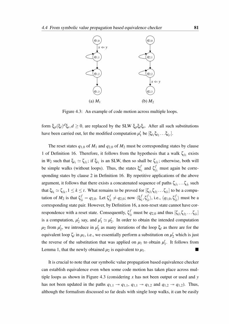
4.4 From symbolic value propagation based equivalence checker 81
(a) M1
q1,0
q1,1
q1,2
q1,3
x⇐ y
(b) M2
q2,0
q2,1
q2,2
q2,3
x⇐ y
Figure 4.3: An example of code motion across multiple loops.
form ξp(ξl)dξs,d ≥ 0, are replaced by the SLW ξpξlξs. After all such substitutions
have been carried out, let the modified computation µ′1 be [ξi1ξi2 . . .ξit′ ].
The reset states q1,0 of M1 and q2,0 of M2 must be corresponding states by clause
1 of Definition 16. Therefore, it follows from the hypothesis that a walk ζ j1 exists
in W2 such that ξi1 ' ζ j1; if ξi1 is an SLW, then so shall be ζ j1; otherwise, both will
be simple walks (without loops). Thus, the states ξfi1 and ζ
fj1 must again be corre-
sponding states by clause 2 in Definition 16. By repetitive applications of the above
argument, it follows that there exists a concatenated sequence of paths ζ j1 . . .ζ jt such
that ξik ' ζ jk ,1≤ k ≤ t. What remains to be proved for [ζ j1ζ j2 . . .ζ jt ] to be a compu-
tation of M2 is that ζfjt = q2,0. Let ζ
fjt 6= q2,0; now 〈ξ f
it ,ζfjt 〉, i.e., 〈q1,0,ζ
fjt 〉 must be a
corresponding state pair. However, by Definition 16, a non-reset state cannot have cor-
respondence with a reset state. Consequently, ζfjt must be q2,0 and thus [ζ j1ζ j2 . . .ζ jt ]
is a computation, µ′2 say, and µ′1 ' µ′2. In order to obtain the intended computation
µ2 from µ′2, we introduce in µ′2 as many iterations of the loop ξl as there are for the
equivalent loop ζl in µ1, i.e., we essentially perform a substitution on µ′2 which is just
the reverse of the substitution that was applied on µ1 to obtain µ′1. It follows from
Lemma 1, that the newly obtained µ2 is equivalent to µ1.
It is crucial to note that our symbolic value propagation based equivalence checker
can establish equivalence even when some code motion has taken place across mul-
tiple loops as shown in Figure 4.3 (considering x has not been output or used and y
has not been updated in the paths q1,1 q1,1, q1,1 q1,2 and q1,2 q1,2). Thus,
although the formalism discussed so far deals with single loop walks, it can be easily
82 Chapter 4 Deriving Bisimulation Relations
extended to accommodate multiple loop walks; for this, the definition of walk cover
(Definition 17), its corresponding Lemma 1, Theorem 7 and their proofs can be suit-
ably extended. Note that the definition of walk given in Definition 14 requires no
modification to incorporate the notion of multiple loop walks.
Next, to establish that the symbolic value propagation based equivalence checker
yields a simulation relation, we define, in the following, another verification relation
accommodating the notion of walks (as given in Definition 14).
Definition 18 (Type-II Verification Relation). A type-II verification relation V ′ for two
FSMDs M1 = 〈Q1,q1,0, I,V1,O,τ1,h1〉 and M2 = 〈Q2,q2,0, I,V2,O,τ2,h2〉 is a verifi-
cation relation which satisfies the following two clauses:
1. V ′(q1,0,q2,0, true), and
2. ∀q1,k ∈ Q1, q2,l ∈ Q2[
V ′(q1,k,q2,l,φk,l)⇔∃q1,i ∈ Q1(q1,i ;P1 q1,k) ∧∀q1,i ∈ Q1
q1,i ;P1 q1,k = ξ, say,⇒
∃q2, j ∈ Q2(
q2, j ;P2 q2,l = ζ, say, ∧ ξ' ζ ∧ V ′(q1,i,q2, j,φi, j)) ]
.
Note that if we allow all walks to be only single paths from the path cover, then
Definition 18 boils down to Definition 13, i.e., the latter is a specific case of the more
general Definition 18.
Theorem 8. The verification relation V ′ for two FSMDs M1,M2 is a simulation rela-
tion for M1,M2, i.e., ∀〈q1,i,q2, j,φi, j〉,〈q1,i,q2, j,φi, j〉 ∈ V ′⇒ 〈q1,i,q2, j,φi, j〉 ∈ S.
Proof: For the pair of reset states, 〈q1,0,q2,0, true〉 is in V ′ and also in S by the
respective first clauses in Definition 18 and Definition 11. For 〈q1,k,q2,l,φk,l〉 ∈ V ′,where q1,k 6= q1,0 and q2,l 6= q2,0, by application of clause 2 in Definition 18 in the
forward direction (i.e., along⇒) m times, m ≥ 1, we may conclude that there exists
a sequence of walks ξ1,ξ2, . . . ,ξm, where the paths constituting ξh,1 ≤ h ≤ m, all
belong to P1 and another sequence of walks ζ1,ζ2, . . . ,ζm, where the paths constituting
ζh,1 ≤ h ≤ m, all belong to P2 such that ξs1 = q1,0,ξ
fm = q1,k,ζ
s1 = q2,0,ζ
fm = q2,l and
ξh' ζh,1≤ h≤m; also the corresponding sequence of configurations 〈q1,0,σ1,0〉;ξ1
〈q1,i1,σ1,i1〉;ξ2 · · ·;ξm 〈q1,im = q1,k,σ1,im = σ1,k〉 and 〈q2,0,σ2,0〉;ζ1 〈q2, j1,σ2, j1〉;ζ2 · · ·;ζm 〈q2, jm = q2,l,σ2, jm = σ2,l〉 satisfy the property that 〈q1,ih,q2, jh,φih, jh〉 ∈V ′,1 ≤ h ≤ m. We shall prove that 〈q1,ih,q2, jh,φih, jh〉 ∈ S, for all h,1 ≤ h ≤ m, holds
by induction on h.
4.4 From symbolic value propagation based equivalence checker 83
Basis case (h = 1): In this case, there must exist a single walk q1,0 ;P1 q1,k = ξ1
in M1 and a walk q2,0 ;P2 q2,l = ζ1 in M2 such that ξ1 ' ζ1. Let the walk ξ1
consist of the paths 〈α11,α
21, . . . ,α
t1〉 from P1; similarly, let ζ1 consist of the paths
〈β11,β
21, . . . ,β
t1〉 from P2. Thus, we have σ1,k = sαt
1(s
αt−11
. . .(sα1
1(σ1,0)) . . .) and σ2,l =
sβt1(s
βt−11
. . .(sβ1
1(σ1,0)) . . .) from Definition 14. So, in clause 2 of Definition 11, let
q1,i = q1,0,σ1,i = σ1,0,σ1,k = sαt1(s
αt−11
. . .(sα1
1(σ1,0)) . . .) so that σ1,k ∈ q1,k(v),η1 =
ξ1,q2, j = q2,0,σ2, j = σ2,0. We notice that the antecedents of clause 2 in Definition 11
hold; specifically, the antecedent 〈q1,0,σ1,0〉;η1 〈q1,k,σ1,k〉 holds by the right hand
side (rhs) of clause 2 in Definition 18; the antecedent φ0,0(σ1,0,σ2,0) holds since φ0,0
is identically true; 〈q1,0,q2,0,φ0,0〉 ∈ S by clause 1 in Definition 11. Hence, the conse-
quents of clause 2 in Definition 11 hold with σ2,l = sβt1(s
βt−11
. . .(sβ1
1(σ1,0)) . . .),η2 =
ζ1; so from the fourth consequent, we have 〈q1,k,q2,l,φk,l〉 ∈ S.
Induction hypothesis: Let 〈q1,k,q2,l,φk,l〉 ∈ S hold whenever the states q1,k in Q1 and
q2,l in Q2 are reachable from q1,0 and q2,0, respectively, through sequences of length
n of pairwise equivalent walks from P1 and P2.
Induction step: Let the state q1,k be reachable from q1,0 through the sequence q1,0 ;ξ1
q1,i1 ;ξ2 · · · ;ξn q1,in ;ξn+1 q1,k in M1 and the state q2,l be reachable from q2,0
through the sequence q2,0 ;ζ1 q2, j1 ;ζ2 · · · ;ζn q2, jn ;ζn+1 q2,l in M2 such that
ξh ' ζh,1 ≤ h ≤ n+ 1. Now 〈q1,in,q2, jn,φin, jn〉 ∈ S by the induction hypothesis. Let
ξn+1 consist of the paths 〈α1n+1,α
2n+1, . . . ,α
t ′n+1〉 from P1; similarly, let ζn+1 consist of
the paths 〈β1n+1,β
2n+1, . . . ,β
t ′n+1〉 from P2. So, in clause 2 in Definition 11, let q1,i =
q1,in,σ1,i = σ1,in,σ1,k = sαt′
n+1(s
αt′−1n+1
. . .(sα1
n+1(σ1,in)) . . .) so that σ1,k = q1,k(v),η1 =
ξn+1,q2, j = q2, jn ,σ2, j = σ2, jn . We notice that the antecedent 〈q1,in,σ1,in〉;η1 〈q1,k,
σ1,k〉 holds by the rhs of clause 2 in Definition 18; the antecedents φin, jn(σ1,in ,σ2, jn)
and 〈q1,in ,q2, jn,φin, jn〉 ∈ S in clause 2 in Definition 18 hold by the induction hypothe-
sis. Hence, the consequents of clause 2 in Definition 11 hold with σ2,l = sβt′
n+1(s
βt′−1n+1
. . .
(sβ1
n+1(σ2, jn)) . . .),η2 = ζn+1; so from the fourth consequent, we have 〈q1,k,q2,l,φk,l〉 ∈
S.
The following theorem captures the fact that symbolic value propagation based
equivalence checking leads to a simulation relation between two FSMDs.
Theorem 9. If a symbolic value propagation based equivalence checker declares an
FSMD M1 to be contained in another FSMD M2 for a path cover P1 of M1, then there is
a simulation relation between M1 and M2 corresponding to the state correspondence
relation δ produced by the equivalence checker. Symbolically,
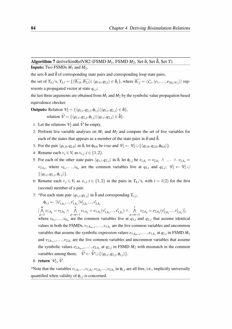
84 Chapter 4 Deriving Bisimulation Relations
Algorithm 7 deriveSimRelVR2 (FSMD M1, FSMD M2, Set δ, Set δ, Set ϒ)Inputs: Two FSMDs M1 and M2,
the sets δ and δ of corresponding state pairs and corresponding loop state pairs,
the set of ϒk,l’s, ϒk,l = 〈ϑ1,k,ϑ2,l〉| 〈q1,k,q2,l〉 ∈ δc, where ϑi, j = 〈C j,〈e1, . . . ,e|V0∪V1|〉〉 rep-
resents a propagated vector at state qi, j;
the last three arguments are obtained from M1 and M2 by the symbolic value propagation based
equivalence checker.
Outputs: Relation V2 = 〈q1,i,q2, j,φi, j〉|〈q1,i,q2, j〉 ∈ δ,relation V = 〈q1,i,q2, j,φi, j〉|〈q1,i,q2, j〉 ∈ δ.
1: Let the relations V2 and V be empty.
2: Perform live variable analyses on M1 and M2 and compute the set of live variables for
each of the states that appears as a member of the state pairs in δ and δ.
3: For the pair 〈q1,0,q2,0〉 in δ, let φ0,0 be true and V2← V2∪〈q1,0,q2,0,φ0,0〉.4: Rename each v j ∈Vi as vi, j, i ∈ 1,2.5: For each of the other state pairs 〈q1,i,q2, j〉 in δ, let φi, j be v1,k1 = v2,k1 ∧ . . . ∧ v1,kn =
v2,kn , where vk1 , . . . ,vkn are the common variables live at q1,i and q2, j; V2 ← V2 ∪〈q1,i,q2, j,φi, j〉.
6: Rename each v j ∈ Vi as vi, j, i ∈ 1,2 in the pairs in ϒk,l’s, with i = 1(2) for the first
(second) member of a pair.
7: *For each state pair 〈q1,i,q2, j〉 in δ and corresponding ϒi, j,
φi, j← ∃v′1,h1, ..,v′1,hx
∃v′2,h1, ..,v′2,hy
[m∧
g=1v1,hg = v2,hg ∧
x∧g=m+1
v1,hg = e1,hg(v′1,h1
, ..,v′1,hx) ∧
y∧g=m+1
v2,hg = e2,hg(v′2,h1
, ..,v′2,hy)],
where vh1 , . . . ,vhm are the common variables live at q1,i and q2, j that assume identical
values in both the FSMDs, v1,hm+1 , . . . ,v1,hx are the live common variables and uncommon
variables that assume the symbolic expression values e1,hm+1 , . . . ,e1,hx at q1,i in FSMD M1
and v2,hx+1 , . . . ,v2,hy are the live common variables and uncommon variables that assume
the symbolic values e2,hm+1 , . . . ,e2,hy at q2, j in FSMD M2 with mismatch in the common
variables among them; V ← V ∪〈q1,i,q2, j,φi, j〉.8: return V2, V .
*Note that the variables v1,h1 , ..,v1,hx ,v2,h1 , ..,v2,hy in φi, j are all free, i.e., implicitly universally
quantified when validity of φi, j is concerned.
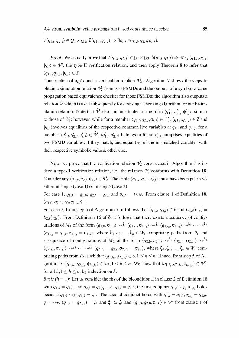
4.4 From symbolic value propagation based equivalence checker 85
∀〈q1,i,q2, j〉 ∈ Q1×Q2, δ(q1,i,q2, j)⇒∃φi, j S(q1,i,q2, j,φi, j).
Proof: We actually prove that ∀〈q1,i,q2, j〉 ∈Q1×Q2, δ(q1,i,q2, j)⇒∃φi, j 〈q1,i,q2, j,
φi, j〉 ∈ V ′, the type-II verification relation, and then apply Theorem 8 to infer that
〈q1,i,q2, j,φi, j〉 ∈ S.
Construction of φi, j ’s and a verification relation V2: Algorithm 7 shows the steps to
obtain a simulation relation V2 from two FSMDs and the outputs of a symbolic value
propagation based equivalence checker for those FSMDs; the algorithm also outputs a
relation V which is used subsequently for devising a checking algorithm for our bisim-
ulation relation. Note that V also contains tuples of the form 〈q′1,i,q′2, j,φ′i, j〉, similar
to those of V2; however, while for a member 〈q1,i,q2, j,φi, j〉 ∈ V2, 〈q1,i,q2, j〉 ∈ δ and
φi, j involves equalities of the respective common live variables at q1,i and q2, j, for a
member 〈q′1,i,q′2, j,φ′i, j〉 ∈ V , 〈q′1,i,q′2, j〉 belongs to δ and φ′i, j comprises equalities of
two FSMD variables, if they match, and equalities of the mismatched variables with
their respective symbolic values, otherwise.
Now, we prove that the verification relation V2 constructed in Algorithm 7 is in-
deed a type-II verification relation, i.e., the relation V2 conforms with Definition 18.
Consider any 〈q1,k,q2,l,φk,l〉 ∈V2. The triple 〈q1,k,q2,l,φk,l〉must have been put in V2
either in step 3 (case 1) or in step 5 (case 2).
For case 1, q1,k = q1,0, q2,l = q2,0 and φk,l = true. From clause 1 of Definition 18,
〈q1,0,q2,0, true〉 ∈ V ′.For case 2, from step 5 of Algorithm 7, it follows that 〈q1,k,q2,l〉 ∈ δ and L1,k(v1c) =
L2,l(v2c). From Definition 16 of δ, it follows that there exists a sequence of config-
urations of M1 of the form 〈q1,0,σ1,0〉;ξ1 〈q1,i1 ,σ1,i1〉;ξ2 〈q1,i2,σ1,i2〉;ξ3 · · ·;ξn
〈q1,in = q1,k,σ1,in = σ1,k〉, where ξ1,ξ2, . . . ,ξn ∈W1 comprising paths from P1 and
a sequence of configurations of M2 of the form 〈q2,0,σ2,0〉 ;ζ1 〈q2, j1,σ2, j1〉 ;ζ2
〈q2, j2 ,σ2, j2〉;ζ3 · · ·;ζn 〈q2, jn = q2,l,σ2, jn = σ2,l〉, where ζ1,ζ2, . . . ,ζn ∈W2 com-
prising paths from P2, such that 〈q1,ih,q2, jh〉 ∈ δ,1≤ h≤ n. Hence, from step 5 of Al-
gorithm 7, 〈q1,ih ,q2, jh,φih, jh〉 ∈ V2,1 ≤ h ≤ n. We show that 〈q1,ih,q2, jh,φih, jh〉 ∈ V ′,for all h,1≤ h≤ n, by induction on h.
Basis (h = 1): Let us consider the rhs of the biconditional in clause 2 of Definition 18
with q1,k = q1,i1 and q2,l = q2, j1 . Let q1,i = q1,0; the first conjunct q1,i ;P1 q1,i1 holds
because q1,0 ;P1 q1,k = ξ1. The second conjunct holds with q1,i = q1,0,q2, j = q2,0,
q2,0 ;P2 (q2,k = q2, j1) = ζ1 and ξ1 ' ζ1 and 〈q1,0,q2,0,φ0,0〉 ∈ V ′ from clause 1 of
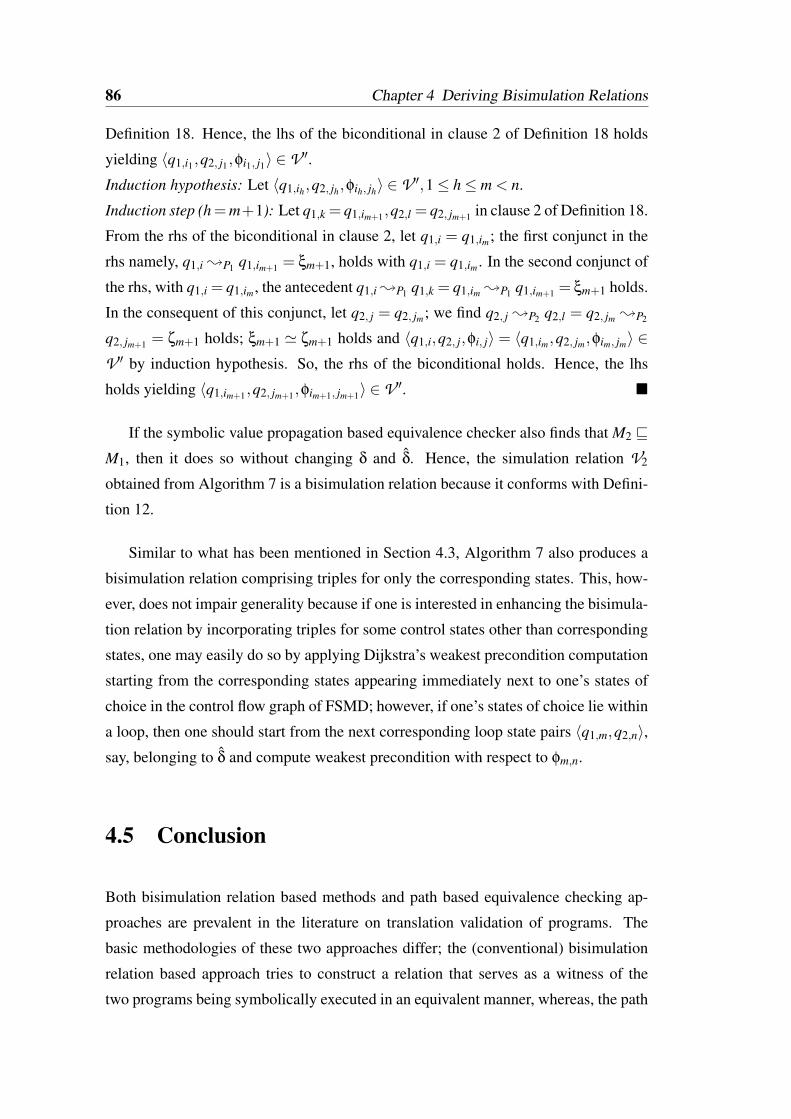
86 Chapter 4 Deriving Bisimulation Relations
Definition 18. Hence, the lhs of the biconditional in clause 2 of Definition 18 holds
yielding 〈q1,i1,q2, j1,φi1, j1〉 ∈ V ′.Induction hypothesis: Let 〈q1,ih ,q2, jh,φih, jh〉 ∈ V ′,1≤ h≤ m < n.
Induction step (h=m+1): Let q1,k = q1,im+1 ,q2,l = q2, jm+1 in clause 2 of Definition 18.
From the rhs of the biconditional in clause 2, let q1,i = q1,im; the first conjunct in the
rhs namely, q1,i ;P1 q1,im+1 = ξm+1, holds with q1,i = q1,im . In the second conjunct of
the rhs, with q1,i = q1,im , the antecedent q1,i ;P1 q1,k = q1,im ;P1 q1,im+1 = ξm+1 holds.
In the consequent of this conjunct, let q2, j = q2, jm; we find q2, j ;P2 q2,l = q2, jm ;P2
q2, jm+1 = ζm+1 holds; ξm+1 ' ζm+1 holds and 〈q1,i,q2, j,φi, j〉 = 〈q1,im ,q2, jm ,φim, jm〉 ∈V ′ by induction hypothesis. So, the rhs of the biconditional holds. Hence, the lhs
holds yielding 〈q1,im+1,q2, jm+1,φim+1, jm+1〉 ∈ V ′.
If the symbolic value propagation based equivalence checker also finds that M2 vM1, then it does so without changing δ and δ. Hence, the simulation relation V2
obtained from Algorithm 7 is a bisimulation relation because it conforms with Defini-
tion 12.
Similar to what has been mentioned in Section 4.3, Algorithm 7 also produces a
bisimulation relation comprising triples for only the corresponding states. This, how-
ever, does not impair generality because if one is interested in enhancing the bisimula-
tion relation by incorporating triples for some control states other than corresponding
states, one may easily do so by applying Dijkstra’s weakest precondition computation
starting from the corresponding states appearing immediately next to one’s states of
choice in the control flow graph of FSMD; however, if one’s states of choice lie within
a loop, then one should start from the next corresponding loop state pairs 〈q1,m,q2,n〉,say, belonging to δ and compute weakest precondition with respect to φm,n.
4.5 Conclusion
Both bisimulation relation based methods and path based equivalence checking ap-
proaches are prevalent in the literature on translation validation of programs. The
basic methodologies of these two approaches differ; the (conventional) bisimulation
relation based approach tries to construct a relation that serves as a witness of the
two programs being symbolically executed in an equivalent manner, whereas, the path

4.5 Conclusion 87
based approach tries to obtain path covers in the two FSMDs such that each path in
one is found to be equivalent with a path in the other and vice-versa. In this chapter,
we relate these two (apparently different) approaches by explaining how bisimula-
tion relations can be derived from the outputs of two types of path based equivalence
checkers namely, a path extension based checker and a symbolic value propagation
based checker. None of the bisimulation relation based approaches has been shown
to tackle code motions across loops; therefore, the present work demonstrates, for the
first time, that a bisimulation relation exists even under such a context when such code
motions are valid. Developing a unified framework that encompasses all the benefits
of these two approaches seems to be an interesting future work.

Chapter 5
Translation Validation of Code MotionTransformations in Array-IntensivePrograms
5.1 Introduction
In Chapter 3, we have presented a symbolic value propagation based equivalence
checking for the FSMD model. A significant deficiency of this method is its inability
to handle an important class of programs, namely those involving arrays. The data
flow analysis for array-intensive programs is notably more complex than those in-
volving only scalars. To illustrate the fact, let us consider two sequential statements
a[i]⇐ 10 and a[ j]⇐ 20. Now consider the scenario where i = j holds, in this case
the second statement qualifies as an overwrite, whereas in the complement scenario
of i 6= j, it does not. Unavailability of relevant information to resolve such relation-
ships between index variables may result in an exponential number of case analyses.
In addition, obtaining the condition of execution and the data transformation of a path
by applying simple substitution as outlined by Dijkstra’s weakest precondition com-
putation may become more expensive in the presence of arrays; conditional clauses
need to be associated depicting equality/non-equality of the index expressions of the
array references in the predicate as it gets transformed through the array assignment
statements in the path.
89
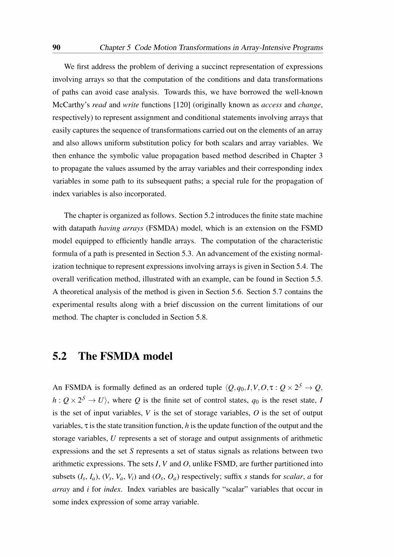
90 Chapter 5 Code Motion Transformations in Array-Intensive Programs
We first address the problem of deriving a succinct representation of expressions
involving arrays so that the computation of the conditions and data transformations
of paths can avoid case analysis. Towards this, we have borrowed the well-known
McCarthy’s read and write functions [120] (originally known as access and change,
respectively) to represent assignment and conditional statements involving arrays that
easily captures the sequence of transformations carried out on the elements of an array
and also allows uniform substitution policy for both scalars and array variables. We
then enhance the symbolic value propagation based method described in Chapter 3
to propagate the values assumed by the array variables and their corresponding index
variables in some path to its subsequent paths; a special rule for the propagation of
index variables is also incorporated.
The chapter is organized as follows. Section 5.2 introduces the finite state machine
with datapath having arrays (FSMDA) model, which is an extension on the FSMD
model equipped to efficiently handle arrays. The computation of the characteristic
formula of a path is presented in Section 5.3. An advancement of the existing normal-
ization technique to represent expressions involving arrays is given in Section 5.4. The
overall verification method, illustrated with an example, can be found in Section 5.5.
A theoretical analysis of the method is given in Section 5.6. Section 5.7 contains the
experimental results along with a brief discussion on the current limitations of our
method. The chapter is concluded in Section 5.8.
5.2 The FSMDA model
An FSMDA is formally defined as an ordered tuple 〈Q,q0, I,V,O,τ : Q× 2S → Q,
h : Q× 2S → U〉, where Q is the finite set of control states, q0 is the reset state, I
is the set of input variables, V is the set of storage variables, O is the set of output
variables, τ is the state transition function, h is the update function of the output and the
storage variables, U represents a set of storage and output assignments of arithmetic
expressions and the set S represents a set of status signals as relations between two
arithmetic expressions. The sets I, V and O, unlike FSMD, are further partitioned into
subsets (Is, Ia), (Vs, Va, Vi) and (Os, Oa) respectively; suffix s stands for scalar, a for
array and i for index. Index variables are basically “scalar” variables that occur in
some index expression of some array variable.
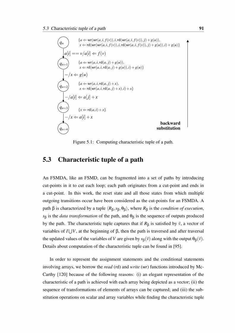
5.3 Characteristic tuple of a path 91
a[i] == v/a[i]⇐ f (v)
−/x⇐ g(u)
−/a[i]⇐ a[ j]+ x
−/x⇐ a[i]+ x
qn
qn+1
qn+2
qn+3
qn+4
a⇐ wr(a, i, rd(a, j)+ x),
a⇐ wr(a, i, rd(a, j)+g(u)),
a⇐ wr(wr(a, i, f (v)), i, rd(wr(a, i, f (v)), j)+g(u)),
x⇐ rd(a, i)+ x
backward
x⇐ rd(wr(wr(a, i, f (v)), i, rd(wr(a, i, f (v)), j)+g(u)), i)+g(u)
x⇐ rd(wr(a, i, rd(a, j)+g(u)), i)+g(u)
x⇐ rd(wr(a, i, rd(a, j)+ x), i)+ x
substitution
Figure 5.1: Computing characteristic tuple of a path.
5.3 Characteristic tuple of a path
An FSMDA, like an FSMD, can be fragmented into a set of paths by introducing
cut-points in it to cut each loop; each path originates from a cut-point and ends in
a cut-point. In this work, the reset state and all those states from which multiple
outgoing transitions occur have been considered as the cut-points for an FSMDA. A
path β is characterized by a tuple 〈Rβ,sβ,θβ〉, where Rβ is the condition of execution,
sβ is the data transformation of the path, and θβ is the sequence of outputs produced
by the path. The characteristic tuple captures that if Rβ is satisfied by v, a vector of
variables of I⋃
V , at the beginning of β, then the path is traversed and after traversal
the updated values of the variables of V are given by sβ(v) along with the output θβ(v).
Details about computation of the characteristic tuple can be found in [95].
In order to represent the assignment statements and the conditional statements
involving arrays, we borrow the read (rd) and write (wr) functions introduced by Mc-
Carthy [120] because of the following reasons: (i) an elegant representation of the
characteristic of a path is achieved with each array being depicted as a vector; (ii) the
sequence of transformations of elements of arrays can be captured; and (iii) the sub-
stitution operations on scalar and array variables while finding the characteristic tuple
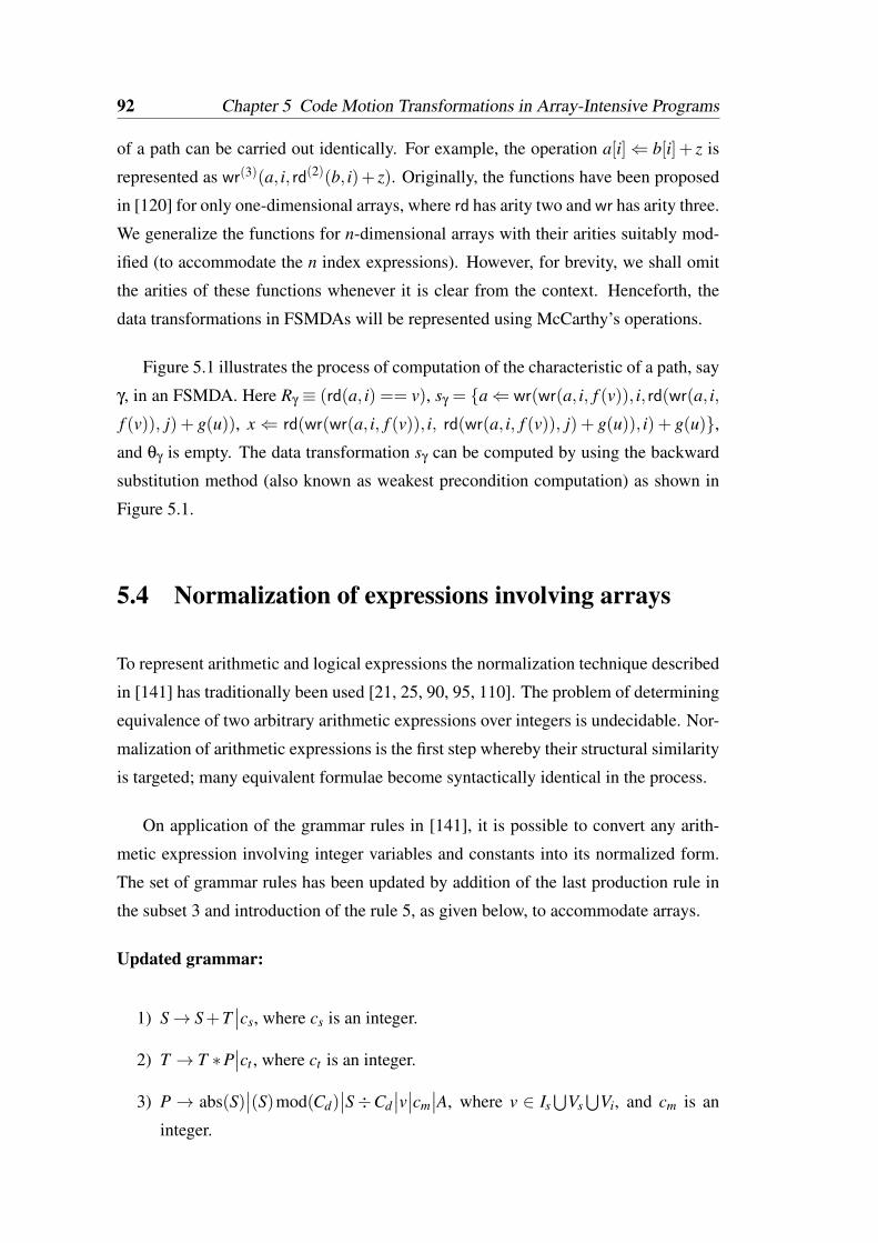
92 Chapter 5 Code Motion Transformations in Array-Intensive Programs
of a path can be carried out identically. For example, the operation a[i]⇐ b[i]+ z is
represented as wr(3)(a, i, rd(2)(b, i)+ z). Originally, the functions have been proposed
in [120] for only one-dimensional arrays, where rd has arity two and wr has arity three.
We generalize the functions for n-dimensional arrays with their arities suitably mod-
ified (to accommodate the n index expressions). However, for brevity, we shall omit
the arities of these functions whenever it is clear from the context. Henceforth, the
data transformations in FSMDAs will be represented using McCarthy’s operations.
Figure 5.1 illustrates the process of computation of the characteristic of a path, say
γ, in an FSMDA. Here Rγ ≡ (rd(a, i) == v), sγ = a⇐ wr(wr(a, i, f (v)), i, rd(wr(a, i,
f (v)), j) + g(u)), x⇐ rd(wr(wr(a, i, f (v)), i, rd(wr(a, i, f (v)), j) + g(u)), i) + g(u),and θγ is empty. The data transformation sγ can be computed by using the backward
substitution method (also known as weakest precondition computation) as shown in
Figure 5.1.
5.4 Normalization of expressions involving arrays
To represent arithmetic and logical expressions the normalization technique described
in [141] has traditionally been used [21, 25, 90, 95, 110]. The problem of determining
equivalence of two arbitrary arithmetic expressions over integers is undecidable. Nor-
malization of arithmetic expressions is the first step whereby their structural similarity
is targeted; many equivalent formulae become syntactically identical in the process.
On application of the grammar rules in [141], it is possible to convert any arith-
metic expression involving integer variables and constants into its normalized form.
The set of grammar rules has been updated by addition of the last production rule in
the subset 3 and introduction of the rule 5, as given below, to accommodate arrays.
Updated grammar:
1) S→ S+T∣∣cs, where cs is an integer.
2) T → T ∗P∣∣ct , where ct is an integer.
3) P → abs(S)∣∣(S)mod(Cd)
∣∣S÷Cd∣∣v∣∣cm
∣∣A, where v ∈ Is⋃
Vs⋃
Vi, and cm is an
integer.
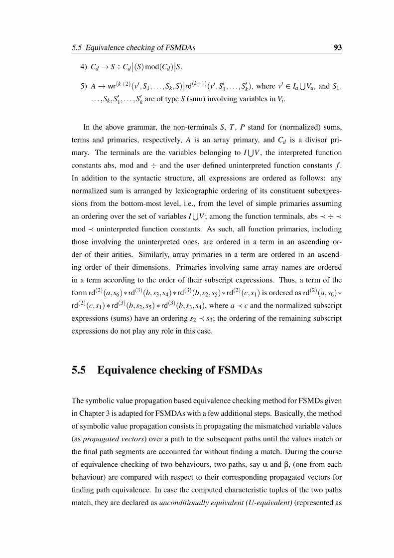
5.5 Equivalence checking of FSMDAs 93
4) Cd → S÷Cd∣∣(S)mod(Cd)
∣∣S.
5) A→ wr(k+2)(v′,S1, . . . ,Sk,S)∣∣rd(k+1)(v′,S′1, . . . ,S
′k), where v′ ∈ Ia
⋃Va, and S1,
. . . ,Sk,S′1, . . . ,S′k are of type S (sum) involving variables in Vi.
In the above grammar, the non-terminals S, T , P stand for (normalized) sums,
terms and primaries, respectively, A is an array primary, and Cd is a divisor pri-
mary. The terminals are the variables belonging to I⋃
V , the interpreted function
constants abs, mod and ÷ and the user defined uninterpreted function constants f .
In addition to the syntactic structure, all expressions are ordered as follows: any
normalized sum is arranged by lexicographic ordering of its constituent subexpres-
sions from the bottom-most level, i.e., from the level of simple primaries assuming
an ordering over the set of variables I⋃
V ; among the function terminals, abs ≺ ÷ ≺mod ≺ uninterpreted function constants. As such, all function primaries, including
those involving the uninterpreted ones, are ordered in a term in an ascending or-
der of their arities. Similarly, array primaries in a term are ordered in an ascend-
ing order of their dimensions. Primaries involving same array names are ordered
in a term according to the order of their subscript expressions. Thus, a term of the
form rd(2)(a,s6)∗ rd(3)(b,s3,s4)∗ rd(3)(b,s2,s5)∗ rd(2)(c,s1) is ordered as rd(2)(a,s6)∗rd(2)(c,s1)∗ rd(3)(b,s2,s5)∗ rd(3)(b,s3,s4), where a ≺ c and the normalized subscript
expressions (sums) have an ordering s2 ≺ s3; the ordering of the remaining subscript
expressions do not play any role in this case.
5.5 Equivalence checking of FSMDAs
The symbolic value propagation based equivalence checking method for FSMDs given
in Chapter 3 is adapted for FSMDAs with a few additional steps. Basically, the method
of symbolic value propagation consists in propagating the mismatched variable values
(as propagated vectors) over a path to the subsequent paths until the values match or
the final path segments are accounted for without finding a match. During the course
of equivalence checking of two behaviours, two paths, say α and β, (one from each
behaviour) are compared with respect to their corresponding propagated vectors for
finding path equivalence. In case the computed characteristic tuples of the two paths
match, they are declared as unconditionally equivalent (U-equivalent) (represented as
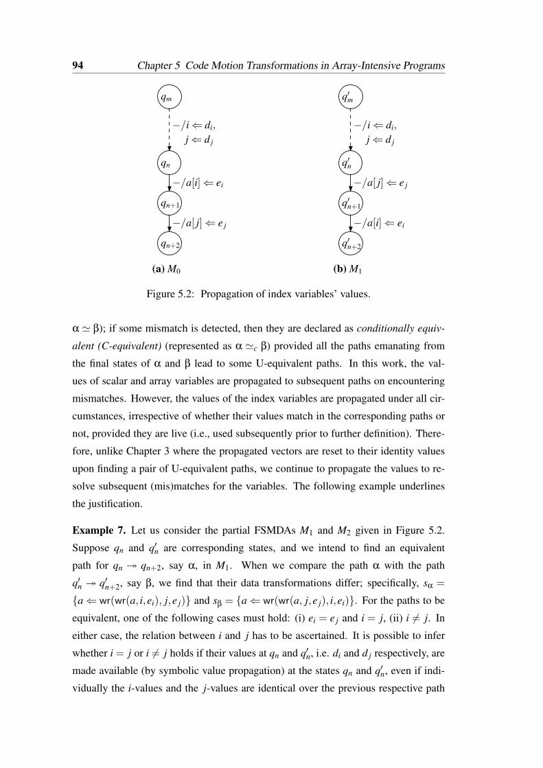
94 Chapter 5 Code Motion Transformations in Array-Intensive Programs
q′m
q′n
q′n+1
q′n+2
(b) M1
−/a[ j]⇐ e j
−/a[i]⇐ ei
−/i⇐ di,
j⇐ d j
qm
qn
qn+1
qn+2
(a) M0
−/a[i]⇐ ei
−/a[ j]⇐ e j
−/i⇐ di,
j⇐ d j
Figure 5.2: Propagation of index variables’ values.
α ' β); if some mismatch is detected, then they are declared as conditionally equiv-
alent (C-equivalent) (represented as α 'c β) provided all the paths emanating from
the final states of α and β lead to some U-equivalent paths. In this work, the val-
ues of scalar and array variables are propagated to subsequent paths on encountering
mismatches. However, the values of the index variables are propagated under all cir-
cumstances, irrespective of whether their values match in the corresponding paths or
not, provided they are live (i.e., used subsequently prior to further definition). There-
fore, unlike Chapter 3 where the propagated vectors are reset to their identity values
upon finding a pair of U-equivalent paths, we continue to propagate the values to re-
solve subsequent (mis)matches for the variables. The following example underlines
the justification.
Example 7. Let us consider the partial FSMDAs M1 and M2 given in Figure 5.2.
Suppose qn and q′n are corresponding states, and we intend to find an equivalent
path for qn qn+2, say α, in M1. When we compare the path α with the path
q′n q′n+2, say β, we find that their data transformations differ; specifically, sα =
a⇐ wr(wr(a, i,ei), j,e j) and sβ = a⇐ wr(wr(a, j,e j), i,ei). For the paths to be
equivalent, one of the following cases must hold: (i) ei = e j and i = j, (ii) i 6= j. In
either case, the relation between i and j has to be ascertained. It is possible to infer
whether i = j or i 6= j holds if their values at qn and q′n, i.e. di and d j respectively, are
made available (by symbolic value propagation) at the states qn and q′n, even if indi-
vidually the i-values and the j-values are identical over the previous respective path
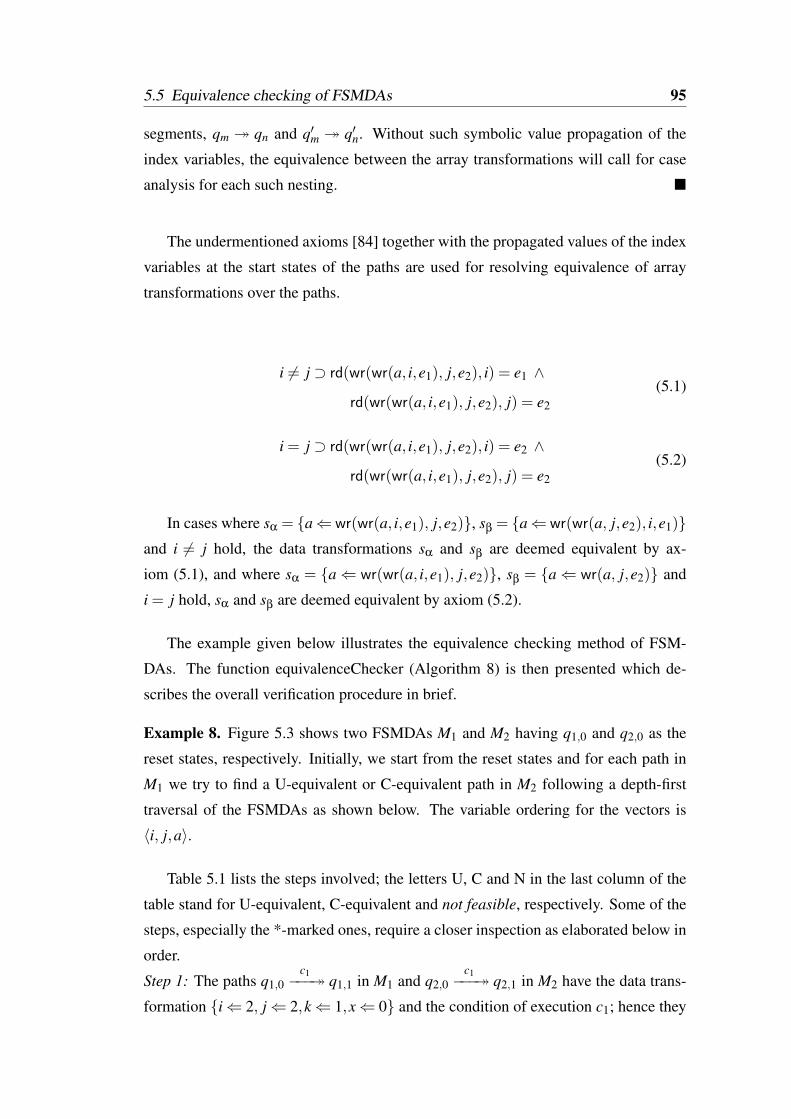
5.5 Equivalence checking of FSMDAs 95
segments, qm qn and q′m q′n. Without such symbolic value propagation of the
index variables, the equivalence between the array transformations will call for case
analysis for each such nesting.
The undermentioned axioms [84] together with the propagated values of the index
variables at the start states of the paths are used for resolving equivalence of array
transformations over the paths.
i 6= j ⊃ rd(wr(wr(a, i,e1), j,e2), i) = e1 ∧
rd(wr(wr(a, i,e1), j,e2), j) = e2
(5.1)
i = j ⊃ rd(wr(wr(a, i,e1), j,e2), i) = e2 ∧
rd(wr(wr(a, i,e1), j,e2), j) = e2
(5.2)
In cases where sα = a⇐ wr(wr(a, i,e1), j,e2), sβ = a⇐ wr(wr(a, j,e2), i,e1)and i 6= j hold, the data transformations sα and sβ are deemed equivalent by ax-
iom (5.1), and where sα = a⇐ wr(wr(a, i,e1), j,e2), sβ = a⇐ wr(a, j,e2) and
i = j hold, sα and sβ are deemed equivalent by axiom (5.2).
The example given below illustrates the equivalence checking method of FSM-
DAs. The function equivalenceChecker (Algorithm 8) is then presented which de-
scribes the overall verification procedure in brief.
Example 8. Figure 5.3 shows two FSMDAs M1 and M2 having q1,0 and q2,0 as the
reset states, respectively. Initially, we start from the reset states and for each path in
M1 we try to find a U-equivalent or C-equivalent path in M2 following a depth-first
traversal of the FSMDAs as shown below. The variable ordering for the vectors is
〈i, j,a〉.
Table 5.1 lists the steps involved; the letters U, C and N in the last column of the
table stand for U-equivalent, C-equivalent and not feasible, respectively. Some of the
steps, especially the *-marked ones, require a closer inspection as elaborated below in
order.
Step 1: The paths q1,0c1−−− q1,1 in M1 and q2,0
c1−−− q2,1 in M2 have the data trans-
formation i⇐ 2, j⇐ 2,k⇐ 1,x⇐ 0 and the condition of execution c1; hence they
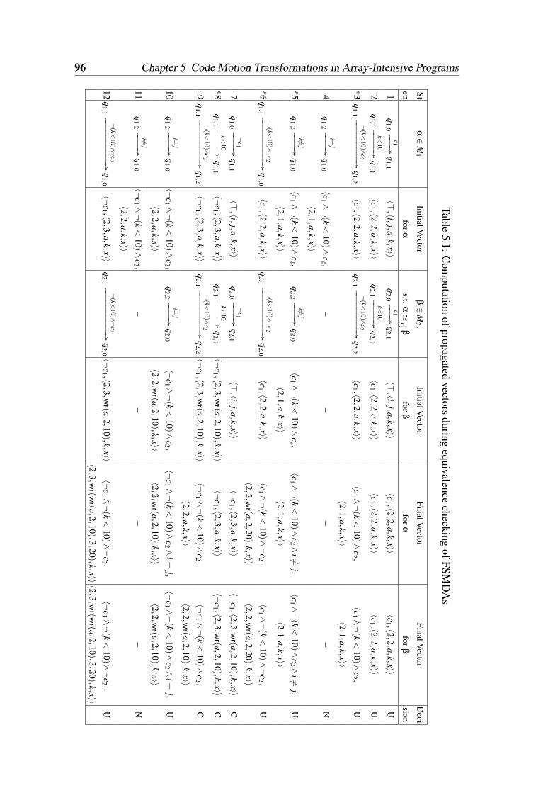
96 Chapter 5 Code Motion Transformations in Array-Intensive Programs
Table5.1:C
omputation
ofpropagatedvectors
duringequivalence
checkingofFSM
DA
s
Stα∈
M1
InitialVector
β∈
M2 ,
InitialVector
FinalVector
FinalVector
Deci
epfor
αs.t.
α'
[c]β
forβ
forα
forβ
sion
1q
1,0c1−−−
q1,1
〈>,〈i,j,a,k,x〉〉
q2,0
c1−−−
q2,1
〈>,〈i,j,a,k,x〉〉
〈c1 ,〈2,2,a,k,x〉〉
〈c1 ,〈2,2,a,k,x〉〉
U
2q
1,1k<
10−−−−−
q1,1
〈c1 ,〈2,2,a,k,x〉〉q
2,1k<
10−−−−−
q2,1
〈c1 ,〈2,2,a,k,x〉〉
〈c1 ,〈2,2,a,k,x〉〉
〈c1 ,〈2,2,a,k,x〉〉
U
*3q
1,1
¬(k<
10)∧
c2−−−−−−−−−
q1,2
〈c1 ,〈2,2,a,k,x〉〉q
2,1¬(k<
10)∧c2
−−−−−−−−−q
2,2〈c1 ,〈2,2,a
,k,x〉〉〈c1 ∧
¬(k
<10
)∧c2 ,
〈c1 ∧¬(k
<10
)∧c2 ,
U
〈2,1,a,k,x〉〉
〈2,1,a,k,x〉〉
4q
1,2i=
j−−−−
q1,0
〈c1 ∧¬(k
<10)∧
c2 ,–
––
–N
〈2,1,a,k,x〉〉
*5q
1,2i6=
j−−−−
q1,0
〈c1 ∧¬(k
<10)∧
c2 ,q
2,2i6=
j−−−−
q2,0
〈c1 ∧¬(k
<10
)∧c2 ,
〈c1 ∧¬(k
<10
)∧c2 ∧
i6=j,
〈c1 ∧¬(k
<10)∧
c2 ∧i6=
j,U
〈2,1,a,k,x〉〉
〈2,1,a,k,x〉〉〈2,1,a
,k,x〉〉〈2,1,a,k,x〉〉
*6q
1,1
¬(k<
10)∧¬
c2−−−−−−−−−−
q1,0
〈c1 ,〈2,2,a,k,x〉〉q
2,1¬(k<
10)∧¬c2
−−−−−−−−−−q
2,0〈c1 ,〈2,2,a
,k,x〉〉〈c1 ∧
¬(k
<10)∧
¬c2 ,
〈c1 ∧¬(k
<10
)∧¬
c2 ,U
〈2,2,wr(a,2,20),k,x〉〉
〈2,2,w
r(a,2,20
),k,x〉〉7
q1,0
¬c1
−−−−q
1,1〈>
,〈i,j,a,k,x〉〉q
2,0¬
c1−−−−
q2,1
〈>,〈i,j,a,k,x〉〉
〈¬c1 ,〈2,3,a,k,x〉〉
〈¬c1 ,〈2,3
,wr(a,2
,10),k,x〉〉
C
*8q
1,1k<
10−−−−−
q1,1
〈¬c1 ,〈2,3
,a,k,x〉〉q
2,1k<
10−−−−−
q2,1
〈¬c1 ,〈2
,3,w
r(a,2,10
),k,x〉〉〈¬
c1 ,〈2,3,a,k,x〉〉〈¬
c1 ,〈2,3,w
r(a,2,10
),k,x〉〉C
9q
1,1
¬(k<
10)∧
c2−−−−−−−−−
q1,2
〈¬c1 ,〈2,3
,a,k,x〉〉q
2,1¬(k<
10)∧c2
−−−−−−−−−q
2,2〈¬
c1 ,〈2,3,w
r(a,2,10
),k,x〉〉〈¬
c1 ∧¬(k
<10)∧
c2 ,〈¬
c1 ∧¬(k
<10
)∧c2 ,
C
〈2,2,a,k,x〉〉
〈2,2,w
r(a,2,10
),k,x〉〉
10q
1,2i=
j−−−−
q1,0
〈¬c1 ∧¬(k
<10
)∧c2 ,
q2,2
i=j
−−−−q
2,0〈¬
c1 ∧¬(k
<10)∧
c2 ,〈¬
c1 ∧¬(k
<10)∧
c2 ∧i=
j,〈¬
c1 ∧¬(k
<10
)∧c2 ∧
i=
j,U
〈2,2,a,k,x〉〉
〈2,2,w
r(a,2,10
),k,x〉〉〈2,2,w
r(a,2,10),k,x〉〉〈2,2,w
r(a,2,10
),k,x〉〉
11q
1,2i6=
j−−−−
q1,0
〈¬c1 ∧¬(k
<10
)∧c2 ,
––
––
N
〈2,2,a,k,x〉〉
12q
1,1
¬(k<
10)∧¬
c2−−−−−−−−−−
q1,0〈¬
c1 ,〈2,3,a,k,x〉〉
q2,1
¬(k<
10)∧¬c2
−−−−−−−−−−q
2,0 〈¬c1 ,〈2
,3,w
r(a,2,10
),k,x〉〉〈¬
c1 ∧¬(k
<10
)∧¬
c2 ,〈¬
c1 ∧¬(k
<10
)∧¬
c2 ,U
〈2,3,wr(w
r(a,2,10
),3,20),k,x〉〉〈2
,3,wr(w
r(a,2,10),3,20),k,x〉〉
5.5 Equivalence checking of FSMDAs 97
q2,0
q2,9
q2,1
q2,4
(b) M2
i 6= j/−
−/a[i]⇐ 10,
¬c1/i⇐ 2,j⇐ 3,
¬c2/a[ j]⇐ 20q2,2
i = j/−
c1/i⇐ 2,j⇐ 2,
x⇐ 0
k⇐ 1,x⇐ 0
c2/ j⇐ j−1
−/−
k⇐ 2,
¬(k < 10)∧
k < 10/
k⇐ k+1x⇐ x+ k,
¬(k < 10)∧
q1,0
q1,3
i 6= j/−
q1,1
q1,4
(a) M1
−/a[ j]⇐ 20
q1,2
i = j/a[ j]⇐ 10
−/−
¬c2/a[i]⇐ 10
¬c1/i⇐ 2,j⇐ 3,
c1/i⇐ 2,j⇐ 2,k⇐ 1,x⇐ 0
k⇐ 2,x⇐ 0
k < 10/x⇐ x+ k,k⇐ k+1
¬(k < 10)∧c2/ j⇐ j−1¬(k < 10)∧
Figure 5.3: An example of equivalence checking of FSMDAs.
are identified to be U-equivalent; however, recursive search for U-equivalent or C-
equivalent paths from the respective final states q1,1 and q2,1 is pursued with the prop-
agated values of the index variables; this permits proper use of the equality antecedents
of the axioms (1) or (2) to simplify data transformations of array elements in the sub-
sequent path segments as explained in Example 7.
Step 2: The simple loops in the respective FSMDAs are now compared. Since their
characteristic tuple match perfectly, these two loops are declared U-equivalent as well.
Step 3: When the paths q1,1¬(k<10)∧c2−−−−−−−−− q1,2 and q2,1
¬(k<10)∧c2−−−−−−−−− q2,2 are com-
pared, a similar decision, as in steps 1 and 2, is taken.
Step 4: The condition for the path q1,2i= j−−−− q1,0 is not satisfied by the propagated
values i⇐ 2, j⇐ 1; specifically, the original Rα ≡ (i = j) and under propagated vec-
tor R′α ≡ (i = j)i/2, j/1 ≡ (2 = 1)≡ false – accordingly, search for a U-equivalent
or C-equivalent path is abandoned through this path for the corresponding propagated
vector.
Step 5: Upon considering the path q1,2i6= j−−−− q1,0, it is found to be U-equivalent with
q2,2i 6= j−−−− q2,0. Since the reset states are reached as the final states of the paths, fur-
ther search for equivalent paths is not pursued.
Step 6: When the paths q1,1¬(k<10)∧¬c2−−−−−−−−−− q1,0 and q2,1
¬(k<10)∧¬c2−−−−−−−−−− q2,0 are com-
pared, their data transformations are found to be i⇐ 2, j⇐ 2,a⇐ wr(wr(a,2,10),
98 Chapter 5 Code Motion Transformations in Array-Intensive Programs
2,20) and i ⇐ 2, j ⇐ 2,a ⇐ wr(a,2,20), respectively. Since i = j, from ax-
iom (5.2), the data transformation of q1,1¬(k<10)∧¬c2−−−−−−−−−− q1,0 can be rewritten as i⇐
2, j⇐ 2,a⇐wr(a,2,20), making it equivalent to that of the path q2,1¬(k<10)∧¬c2−−−−−−−−−−
q2,0. The values for the variable a in both the paths match, and hence its symbolic
value “a” is stored in the final propagated vector. The paths are declared U-equivalent.
Since reset states have been reached, no further search from the respective final state
is needed.
Step 7: The operation a ⇐ wr(a, i,10) in the path q2,0¬c1−−−− q2,1 has no identi-
cal operation in the path q1,0¬c1−−−− q1,1. Therefore, this is the first step where the
transformed propagated vectors mismatch, and hence the two paths are declared to
be candidate C-equivalent. The value for the array a is propagated anticipating that a
similar operation may eventually be discovered in M1 making the subsequent paths U-
equivalent. If all the subsequent paths eventually lead to some U-equivalent path, then
such candidate C-equivalent paths are declared to be C-equivalent; otherwise they are
adjudged to be inequivalent.
Step 8: The loops q1,1k<10−−−−− q1,1 and q2,1
k<10−−−−− q2,1 with propagated vectors
〈¬c1,〈2,3,a,k,x〉〉 (= ϑ, say) and 〈¬c1,〈2,3,wr(a,2,10),k,x〉〉 (= ϑ′), respectively,
are compared; although the characteristic tuples of the loops match, the mismatch in
the value of a persists. Since the propagated vectors obtained during the entry and the
exit of the loop for both the FSMDAs are identical, it indicates that code motion across
loop may have occurred, i.e., if an assignment of the variable a is found in M1 which
renders the values of a in both the FSMDAs equivalent, then such code motion across
loop will indeed be valid. So, these paths are declared as candidate C-equivalent and
the search for U-equivalence is continued.
Step 9: Upon comparing the paths q1,1¬(k<10)∧c2−−−−−−−−− q1,2 and q2,1
¬(k<10)∧c2−−−−−−−−− q2,2,
the matching operation in M1 is still not found, and the values for a along with those
of the index variables are further propagated.
Step 10: The matching operation is finally found in the path q1,2i= j−−−− q1,0 mak-
ing its data transformation same as that of q2,2i= j−−−− q2,0, i.e. i⇐ 2, j⇐ 2,a⇐
wr(a,2,10), confirming a valid code motion across loop and rendering these two
paths U-equivalent.
Step 11: Similar situation as that of step 4 arises, and hence the path q1,2i 6= j−−−− q1,0
is deemed to be not feasible for the corresponding propagated vector.
Step 12: Based on the propagated vectors ϑ and ϑ′ at q1,1 and q2,1, the data trans-
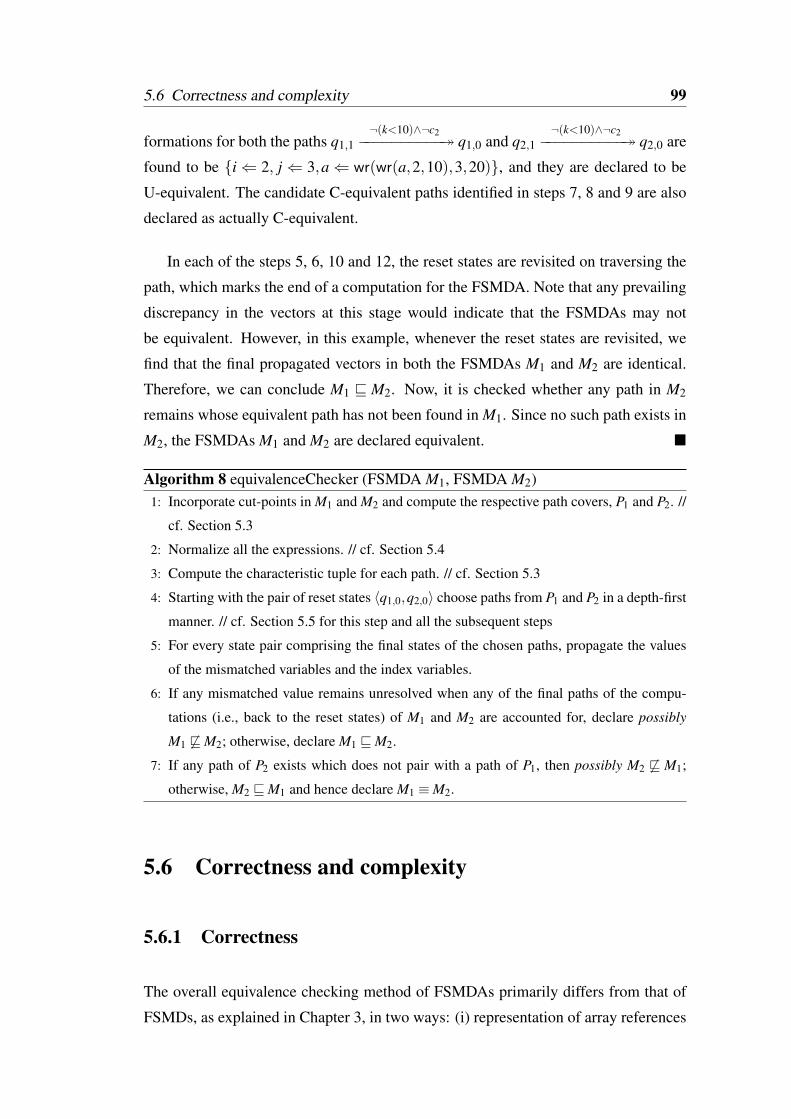
5.6 Correctness and complexity 99
formations for both the paths q1,1¬(k<10)∧¬c2−−−−−−−−−− q1,0 and q2,1
¬(k<10)∧¬c2−−−−−−−−−− q2,0 are
found to be i⇐ 2, j⇐ 3,a⇐ wr(wr(a,2,10),3,20), and they are declared to be
U-equivalent. The candidate C-equivalent paths identified in steps 7, 8 and 9 are also
declared as actually C-equivalent.
In each of the steps 5, 6, 10 and 12, the reset states are revisited on traversing the
path, which marks the end of a computation for the FSMDA. Note that any prevailing
discrepancy in the vectors at this stage would indicate that the FSMDAs may not
be equivalent. However, in this example, whenever the reset states are revisited, we
find that the final propagated vectors in both the FSMDAs M1 and M2 are identical.
Therefore, we can conclude M1 v M2. Now, it is checked whether any path in M2
remains whose equivalent path has not been found in M1. Since no such path exists in
M2, the FSMDAs M1 and M2 are declared equivalent.
Algorithm 8 equivalenceChecker (FSMDA M1, FSMDA M2)1: Incorporate cut-points in M1 and M2 and compute the respective path covers, P1 and P2. //
cf. Section 5.3
2: Normalize all the expressions. // cf. Section 5.4
3: Compute the characteristic tuple for each path. // cf. Section 5.3
4: Starting with the pair of reset states 〈q1,0,q2,0〉 choose paths from P1 and P2 in a depth-first
manner. // cf. Section 5.5 for this step and all the subsequent steps
5: For every state pair comprising the final states of the chosen paths, propagate the values
of the mismatched variables and the index variables.
6: If any mismatched value remains unresolved when any of the final paths of the compu-
tations (i.e., back to the reset states) of M1 and M2 are accounted for, declare possibly
M1 6vM2; otherwise, declare M1 vM2.
7: If any path of P2 exists which does not pair with a path of P1, then possibly M2 6v M1;
otherwise, M2 vM1 and hence declare M1 ≡M2.
5.6 Correctness and complexity
5.6.1 Correctness
The overall equivalence checking method of FSMDAs primarily differs from that of
FSMDs, as explained in Chapter 3, in two ways: (i) representation of array references
100 Chapter 5 Code Motion Transformations in Array-Intensive Programs
using McCarthy’s functions and (ii) propagation on index variable values in spite of
a match. Since none of these modifications has any bearing on the correctness of
the equivalence checking procedure for FSMDAs as compared to that of FSMDs, the
proofs of soundness and termination for Algorithm 8 are explained here intuitively to
avoid repetition.
Soundness: Once the cut-points have been introduced and the path covers have
been constructed (step 1 in Algorithm 8), the equivalence checking method starts
with the reset states and for each path in FSMDA M1 searches for corresponding
U-equivalent or C-equivalent path in the other FSMDA M2 in a depth-first manner
(steps 4 and 5). It declares the two FSMDAs equivalent only when the algorithm suc-
ceeds in finding U-equivalent or C-equivalent path pairs for every path in M1 and M2
(step 7), otherwise the FSMDAs are considered to be possibly non-equivalent (steps 6
and 7). Now, suppose that the algorithm is not sound, i.e., it declares two FSMDAs
to be equivalent when there is a path, γ say, in either of the FSMDAs containing an
operation, e say, whose match does not occur in the other FSMDA. The path γ will
obviously not have a U-equivalent path in the other FSMDA; moreover, it will nei-
ther have a C-equivalent path because, as already mentioned in the beginning of the
previous section, two paths are declared to be C-equivalent only when all the paths em-
anating from their final states lead to some U-equivalent paths, i.e., the mismatched
operation e must have been compensated for eventually in the other FSMDA, which
is a contradiction.
Termination: Since normalization of expressions and computing characteristic
tuples of paths take finite number of steps and the number of paths in an FSMDA is
finite, Algorithm 8 must terminate.
5.6.2 Complexity
Representation of array references by adopting McCarthy’s functions does not change
the complexity of normalization. On the other hand, propagation of variable values
(index or otherwise) has to be done along all possible paths in the worst case, where
the mismatches are not resolved until the last path in an FSMDA has been traversed;
thus, the second difference on account of index variables leads to no ramification
of the worst case time complexity of the equivalence checking method of FSMDAs
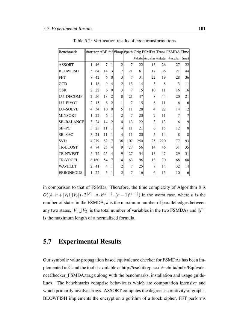
5.7 Experimental Results 101
Table 5.2: Verification results of code transformations
Benchmark #arr #op #BB #if #loop #path Orig FSMDA Trans FSMDA Time
#state #scalar #state #scalar (ms)
ASSORT 1 46 7 1 2 7 22 13 26 27 22
BLOWFISH 5 64 14 3 7 21 61 17 36 21 44
FFT 8 42 6 0 3 7 31 22 19 28 36
GCD 1 18 9 4 2 13 14 3 8 3 11
GSR 2 22 6 0 3 7 15 10 11 16 16
LU–DECOMP 2 56 18 2 8 21 47 8 44 20 21
LU–PIVOT 2 15 6 2 1 7 15 6 11 6 6
LU–SOLVE 4 34 10 0 5 11 28 4 22 14 12
MINSORT 1 22 6 1 2 7 20 7 11 7 7
SB–BALANCE 3 24 14 2 4 13 22 3 13 6 9
SB–PC 3 25 11 1 4 11 21 6 15 12 8
SB–SAC 3 21 11 1 4 11 20 5 14 8 8
SVD 4 279 82 17 36 107 250 25 220 77 93
TR-LCOST 4 74 25 4 9 27 56 14 46 31 35
TR-NWEST 5 72 25 4 9 27 54 13 47 29 31
TR-VOGEL 8 160 54 17 14 63 96 13 70 68 68
WAVELET 2 41 4 1 2 7 25 8 14 32 14
ERRONEOUS 1 22 5 1 2 7 16 6 15 10 6
in comparison to that of FSMDs. Therefore, the time complexity of Algorithm 8 is
O((k · n+ |V1⋃
V2|) · 2‖F‖ · n · k(n−1) · (n− 1)(n−1)) in the worst case, where n is the
number of states in the FSMDA, k is the maximum number of parallel edges between
any two states, |V1⋃
V2| is the total number of variables in the two FSMDAs and ‖F‖is the maximum length of a normalized formula.
5.7 Experimental Results
Our symbolic value propagation based equivalence checker for FSMDAs has been im-
plemented in C and the tool is available at http://cse.iitkgp.ac.in/~chitta/pubs/Equivale-
nceChecker_FSMDA.tar.gz along with the benchmarks, installation and usage guide-
lines. The benchmarks comprise behaviours which are computation intensive and
which primarily involve arrays. ASSORT computes the degree assortativity of graphs,
BLOWFISH implements the encryption algorithm of a block cipher, FFT performs
102 Chapter 5 Code Motion Transformations in Array-Intensive Programs
fast Fourier transform, GCD finds the greatest common divisor of the members of
an array, GSR implements Gauss-Seidel relaxation method, MINSORT is a sorting
function, SVD computes singular value decomposition of a matrix, and WAVELET
implements the Debaucles 4-coefficient wavelet filter. The benchmarks having “LU”
as prefix are concerned with the LU decomposition of a matrix, which is a key step
for several algorithms in linear algebra. The benchmarks having “SB” as prefix test
cryptographic properties like balancedness, PC, and SAC for an S-box [142] whereas,
those with “TR” are the various solutions to the transportation problem namely least
cost method, northwest corner method and Vogel’s approximation method. ERRO-
NEOUS is an example which reveals a bug in the implementation of copy propaga-
tion for array variables in the SPARK [64] tool that was first reported in [103]. These
benchmarks are fed to the SPARK tool to obtain the transformed behaviours. New
scalar variables, but no array variables, are introduced during the transformations.
The proposed method can ascertain the equivalences in all the cases except the last
one; in this case, it reports a possible non-equivalence and outputs a set of paths (each
paired with an almost similar path) for which equivalence could not be found. The
verification results are provided in Table 5.2.
The outputs of SPARK do not contain any “for” loops; the tool converts them into
do-while loops. The tools of [154] and [88] which are existing equivalence checkers
for array-intensive programs require the loops to be represented as “for” loops with
their ranges clearly specified. Hence, the do-while loops in the outputs of the SPARK
tool corresponding to for loops in the original specifications are manually restored to
for loops and given along with the original programs to these tools for equivalence
checking. These tools, however, still failed to establish the equivalence.
5.7.1 Current limitations
The method presented in this work has the following limitations.
(1) Arrays containing other arrays in their subscripts are not allowed. A possible
remedy is to simply allow arrays to appear in Vi; however, our current imple-
mentation does not support it.
(2) It cannot handle loop transformations.
5.8 Conclusion 103
5.8 Conclusion
The literature on behavioural verification is rich with applications of the FSMD model
involving only scalar variables. The model, and hence the verifiers built upon it, can-
not handle arrays. To alleviate this limitation, the current chapter has made the follow-
ing contributions. (i) A new model called FSMDA is introduced which is an extension
of the FSMD model equipped to handle arrays. (ii) An improvisation of the normal-
ization process [141] is suggested to represent arithmetic expressions involving arrays
in normalized forms. (iii) The equivalence checker described in Chapter 3 is fitted
with the FSMDA model to verify code transformations in array-intensive programs.
The experiments carried out on benchmarks from various domains of embedded sys-
tems such as signal processing, data communication, hardware security, etc. attest
the efficacy of the method. Enhancing the present method to overcome the current
limitations stated above remains as our future goal.

Chapter 6
Translation Validation of Loop andArithmetic Transformations in thePresence of Recurrences
6.1 Introduction
Loop transformations together with arithmetic transformations are applied extensively
in the domain of multimedia and signal processing applications to obtain better per-
formance in terms of energy, area and/or execution time [30, 79, 131, 165]. Loop
transformations essentially involve partitioning/unifying the index spaces of arrays.
Figure 6.1 shows two programs before and after application of loop fusion and tiling
transformations. Specifically, two nested loops in the original program are fused into
one and then the 8×8 index space of 〈i, j〉 is covered hierarchically along 4×4 tiles by
the outer loop iterators 〈l1, l2〉, each tile having 2× 2 elements covered by the inner
loop iterators 〈l3, l4〉. Clearly, establishing equivalence/non-equivalence of the two
programs shown in Figure 6.1 calls for an (elaborate) analysis of the index spaces of
the involved arrays. The equivalence checking strategy involving the FSMDA model,
as explained in the previous chapter, is not equipped to handle such reasoning over
array index spaces; rather data dependence graph based analyses have been found to
be suitable for verification of loop transformations.
105
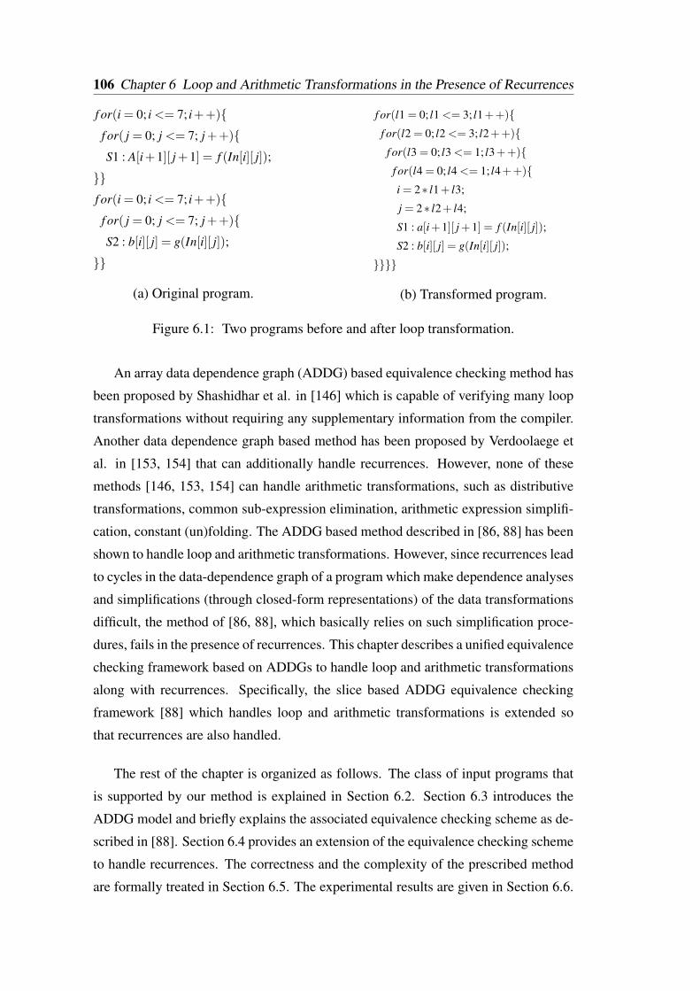
106 Chapter 6 Loop and Arithmetic Transformations in the Presence of Recurrences
f or(i = 0; i <= 7; i++)f or( j = 0; j <= 7; j++)S1 : A[i+1][ j+1] = f (In[i][ j]);
f or(i = 0; i <= 7; i++)f or( j = 0; j <= 7; j++)S2 : b[i][ j] = g(In[i][ j]);
(a) Original program.
f or(l1 = 0; l1 <= 3; l1++)f or(l2 = 0; l2 <= 3; l2++)f or(l3 = 0; l3 <= 1; l3++)
f or(l4 = 0; l4 <= 1; l4++)i = 2∗ l1+ l3;
j = 2∗ l2+ l4;
S1 : a[i+1][ j+1] = f (In[i][ j]);
S2 : b[i][ j] = g(In[i][ j]);
(b) Transformed program.
Figure 6.1: Two programs before and after loop transformation.
An array data dependence graph (ADDG) based equivalence checking method has
been proposed by Shashidhar et al. in [146] which is capable of verifying many loop
transformations without requiring any supplementary information from the compiler.
Another data dependence graph based method has been proposed by Verdoolaege et
al. in [153, 154] that can additionally handle recurrences. However, none of these
methods [146, 153, 154] can handle arithmetic transformations, such as distributive
transformations, common sub-expression elimination, arithmetic expression simplifi-
cation, constant (un)folding. The ADDG based method described in [86, 88] has been
shown to handle loop and arithmetic transformations. However, since recurrences lead
to cycles in the data-dependence graph of a program which make dependence analyses
and simplifications (through closed-form representations) of the data transformations
difficult, the method of [86, 88], which basically relies on such simplification proce-
dures, fails in the presence of recurrences. This chapter describes a unified equivalence
checking framework based on ADDGs to handle loop and arithmetic transformations
along with recurrences. Specifically, the slice based ADDG equivalence checking
framework [88] which handles loop and arithmetic transformations is extended so
that recurrences are also handled.
The rest of the chapter is organized as follows. The class of input programs that
is supported by our method is explained in Section 6.2. Section 6.3 introduces the
ADDG model and briefly explains the associated equivalence checking scheme as de-
scribed in [88]. Section 6.4 provides an extension of the equivalence checking scheme
to handle recurrences. The correctness and the complexity of the prescribed method
are formally treated in Section 6.5. The experimental results are given in Section 6.6.
6.2 The class of supported input programs 107
The chapter is finally concluded in Section 6.7.
6.2 The class of supported input programs
The following restrictions characterize the input programs that can be handled by our
equivalence checking method:
Static control-flow: A control flow of a program that can be exactly determined
at compile time or by some input parameters read at the beginning of the program is
called a static control flow (or data independent control flow). Programs with data
dependent control flow have to be first converted into data independent control flow
to make them amenable for our framework; data dependent while-loops are to be
converted manually to for-loops with worst-case bounds. Restricting to static control
flow is important because of non-availability of tools to determine the dependence
mappings and their domains for data dependent control flow.
Affine indices and bounds: All loop bounds, conditions, and array index expres-
sions of the programs must be affine expressions of the surrounding iterators and sym-
bolic constants. They, however, need not be strictly affine, but can be piece-wise (or
quasi) affine, thus, they can also have mod, div, max, min, floor and ceil operators.
The affine indices and bounds property is critical for the decidability or computability
of many of the operations that we need to perform on sets of integers and mappings
described by constraints expressed as affine functions.
Valid schedule: To satisfy the valid-schedule restriction, each value that is read in
an assignment statement has either been already written or is an input variable. This
is a common requirement in most of the array data-flow analysis methods [12].
Single-assignment form: A behaviour is said to be in single assignment (SA) form
if any memory location is written at most once in the entire behaviour. A program with
static control-flow and with affine indices and bounds can automatically be converted
into an equivalent program in single-assignment form [151].
Other restrictions: In a single-assignment form program, any variable other than
the loop indices, can be replaced with an array variable [144]. Therefore, without
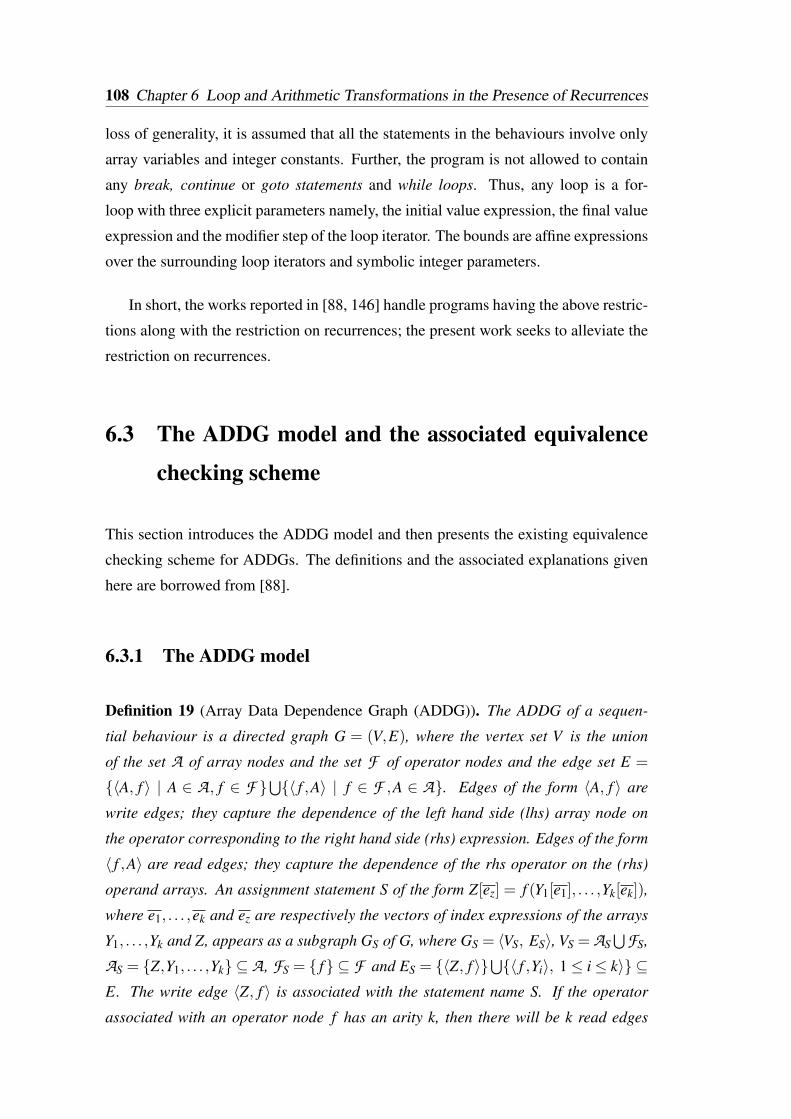
108 Chapter 6 Loop and Arithmetic Transformations in the Presence of Recurrences
loss of generality, it is assumed that all the statements in the behaviours involve only
array variables and integer constants. Further, the program is not allowed to contain
any break, continue or goto statements and while loops. Thus, any loop is a for-
loop with three explicit parameters namely, the initial value expression, the final value
expression and the modifier step of the loop iterator. The bounds are affine expressions
over the surrounding loop iterators and symbolic integer parameters.
In short, the works reported in [88, 146] handle programs having the above restric-
tions along with the restriction on recurrences; the present work seeks to alleviate the
restriction on recurrences.
6.3 The ADDG model and the associated equivalence
checking scheme
This section introduces the ADDG model and then presents the existing equivalence
checking scheme for ADDGs. The definitions and the associated explanations given
here are borrowed from [88].
6.3.1 The ADDG model
Definition 19 (Array Data Dependence Graph (ADDG)). The ADDG of a sequen-
tial behaviour is a directed graph G = (V,E), where the vertex set V is the union
of the set A of array nodes and the set F of operator nodes and the edge set E =
〈A, f 〉 | A ∈ A , f ∈ F ⋃〈 f ,A〉 | f ∈ F ,A ∈ A. Edges of the form 〈A, f 〉 are
write edges; they capture the dependence of the left hand side (lhs) array node on
the operator corresponding to the right hand side (rhs) expression. Edges of the form
〈 f ,A〉 are read edges; they capture the dependence of the rhs operator on the (rhs)
operand arrays. An assignment statement S of the form Z[ez] = f (Y1[e1], . . . ,Yk[ek]),
where e1, . . . ,ek and ez are respectively the vectors of index expressions of the arrays
Y1, . . . ,Yk and Z, appears as a subgraph GS of G, where GS = 〈VS, ES〉, VS = AS⋃
FS,
AS = Z,Y1, . . . ,Yk ⊆ A , FS = f ⊆ F and ES = 〈Z, f 〉⋃〈 f ,Yi〉, 1≤ i≤ k〉 ⊆
E. The write edge 〈Z, f 〉 is associated with the statement name S. If the operator
associated with an operator node f has an arity k, then there will be k read edges
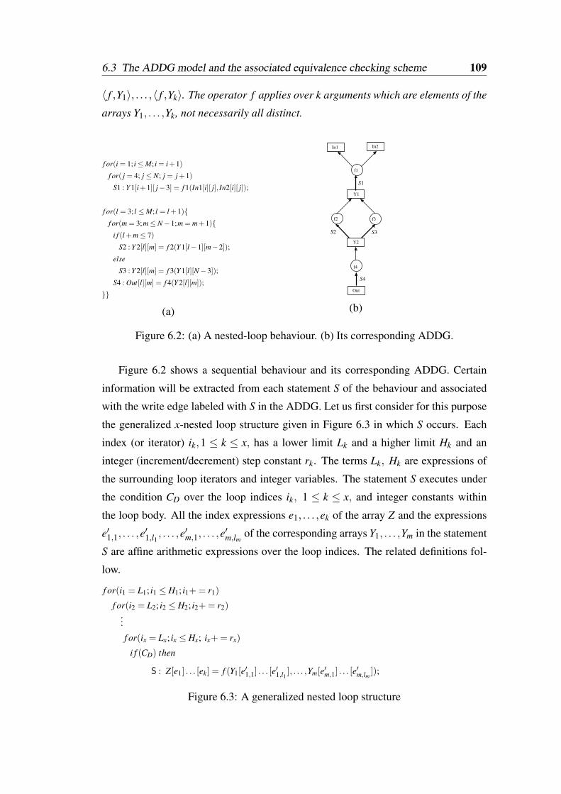
6.3 The ADDG model and the associated equivalence checking scheme 109
〈 f ,Y1〉, . . . ,〈 f ,Yk〉. The operator f applies over k arguments which are elements of the
arrays Y1, . . . ,Yk, not necessarily all distinct.
f or(i = 1; i≤M; i = i+1)
f or( j = 4; j ≤ N; j = j+1)
S1 : Y 1[i+1][ j−3] = f 1(In1[i][ j], In2[i][ j]);
f or(l = 3; l ≤M; l = l +1)f or(m = 3;m≤ N−1;m = m+1)
i f (l +m≤ 7)
S2 : Y 2[l][m] = f 2(Y 1[l−1][m−2]);
else
S3 : Y 2[l][m] = f 3(Y 1[l][N−3]);
S4 : Out[l][m] = f 4(Y 2[l][m]);
(a) (b)
S1
S3
S4
S2
Y2
Y1
In1 In2
f1
f3f2
f4
Out
Figure 6.2: (a) A nested-loop behaviour. (b) Its corresponding ADDG.
Figure 6.2 shows a sequential behaviour and its corresponding ADDG. Certain
information will be extracted from each statement S of the behaviour and associated
with the write edge labeled with S in the ADDG. Let us first consider for this purpose
the generalized x-nested loop structure given in Figure 6.3 in which S occurs. Each
index (or iterator) ik,1 ≤ k ≤ x, has a lower limit Lk and a higher limit Hk and an
integer (increment/decrement) step constant rk. The terms Lk, Hk are expressions of
the surrounding loop iterators and integer variables. The statement S executes under
the condition CD over the loop indices ik, 1 ≤ k ≤ x, and integer constants within
the loop body. All the index expressions e1, . . . ,ek of the array Z and the expressions
e′1,1, . . . ,e′1,l1 , . . . ,e
′m,1, . . . ,e
′m,lm of the corresponding arrays Y1, . . . ,Ym in the statement
S are affine arithmetic expressions over the loop indices. The related definitions fol-
low.
f or(i1 = L1; i1 ≤ H1; i1+= r1)
f or(i2 = L2; i2 ≤ H2; i2+= r2)...
f or(ix = Lx; ix ≤ Hx; ix+= rx)
i f (CD) then
S : Z[e1] . . . [ek] = f (Y1[e′1,1] . . . [e′1,l1
], . . . ,Ym[e′m,1] . . . [e′m,lm ]);
Figure 6.3: A generalized nested loop structure
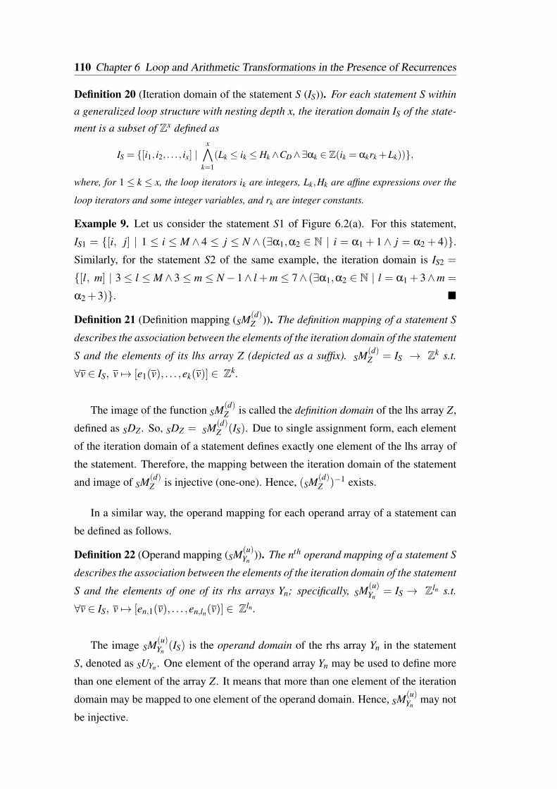
110 Chapter 6 Loop and Arithmetic Transformations in the Presence of Recurrences
Definition 20 (Iteration domain of the statement S (IS)). For each statement S within
a generalized loop structure with nesting depth x, the iteration domain IS of the state-
ment is a subset of Zx defined as
IS = [i1, i2, . . . , ix] |x∧
k=1
(Lk ≤ ik ≤ Hk∧CD∧∃αk ∈ Z(ik = αkrk +Lk)),
where, for 1 ≤ k ≤ x, the loop iterators ik are integers, Lk,Hk are affine expressions over the
loop iterators and some integer variables, and rk are integer constants.
Example 9. Let us consider the statement S1 of Figure 6.2(a). For this statement,
IS1 = [i, j] | 1 ≤ i ≤ M ∧ 4 ≤ j ≤ N ∧ (∃α1,α2 ∈ N | i = α1 + 1∧ j = α2 + 4).Similarly, for the statement S2 of the same example, the iteration domain is IS2 =
[l, m] | 3 ≤ l ≤ M∧ 3 ≤ m ≤ N− 1∧ l +m ≤ 7∧ (∃α1,α2 ∈ N | l = α1 + 3∧m =
α2 +3).
Definition 21 (Definition mapping (SM(d)Z )). The definition mapping of a statement S
describes the association between the elements of the iteration domain of the statement
S and the elements of its lhs array Z (depicted as a suffix). SM(d)Z = IS → Zk s.t.
∀v ∈ IS, v 7→ [e1(v), . . . ,ek(v)] ∈ Zk.
The image of the function SM(d)Z is called the definition domain of the lhs array Z,
defined as SDZ . So, SDZ = SM(d)Z (IS). Due to single assignment form, each element
of the iteration domain of a statement defines exactly one element of the lhs array of
the statement. Therefore, the mapping between the iteration domain of the statement
and image of SM(d)Z is injective (one-one). Hence, (SM(d)
Z )−1 exists.
In a similar way, the operand mapping for each operand array of a statement can
be defined as follows.
Definition 22 (Operand mapping (SM(u)Yn
)). The nth operand mapping of a statement S
describes the association between the elements of the iteration domain of the statement
S and the elements of one of its rhs arrays Yn; specifically, SM(u)Yn
= IS → Zln s.t.
∀v ∈ IS, v 7→ [en,1(v), . . . ,en,ln(v)] ∈ Zln .
The image SM(u)Yn
(IS) is the operand domain of the rhs array Yn in the statement
S, denoted as SUYn . One element of the operand array Yn may be used to define more
than one element of the array Z. It means that more than one element of the iteration
domain may be mapped to one element of the operand domain. Hence, SM(u)Yn
may not
be injective.
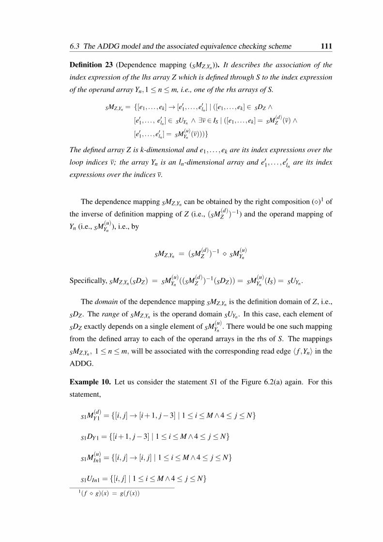
6.3 The ADDG model and the associated equivalence checking scheme 111
Definition 23 (Dependence mapping (SMZ,Yn)). It describes the association of the
index expression of the lhs array Z which is defined through S to the index expression
of the operand array Yn,1≤ n≤ m, i.e., one of the rhs arrays of S.
SMZ,Yn = [e1, . . . ,ek]→ [e′1, . . . ,e′ln ] | ([e1, . . . ,ek] ∈ SDZ ∧
[e′1, . . . , e′ln ] ∈ SUYn ∧ ∃v ∈ IS | ([e1, . . . ,ek] = SM(d)Z (v) ∧
[e′1, . . . ,e′ln ] = SM(u)
Yn(v)))
The defined array Z is k-dimensional and e1, . . . ,ek are its index expressions over the
loop indices v; the array Yn is an ln-dimensional array and e′1, . . . ,e′ln are its index
expressions over the indices v.
The dependence mapping SMZ,Yn can be obtained by the right composition ()1 of
the inverse of definition mapping of Z (i.e., (SM(d)Z )−1) and the operand mapping of
Yn (i.e., SM(u)Yn
), i.e., by
SMZ,Yn = (SM(d)Z )−1 SM(u)
Yn
Specifically, SMZ,Yn(SDZ) = SM(u)Yn
((SM(d)Z )−1(SDZ)) = SM(u)
Yn(IS) = SUYn .
The domain of the dependence mapping SMZ,Yn is the definition domain of Z, i.e.,
SDZ . The range of SMZ,Yn is the operand domain SUYn . In this case, each element of
SDZ exactly depends on a single element of SM(u)Yn
. There would be one such mapping
from the defined array to each of the operand arrays in the rhs of S. The mappings
SMZ,Yn , 1≤ n≤ m, will be associated with the corresponding read edge 〈 f ,Yn〉 in the
ADDG.
Example 10. Let us consider the statement S1 of the Figure 6.2(a) again. For this
statement,
S1M(d)Y 1 = [i, j]→ [i+1, j−3] | 1≤ i≤M∧4≤ j ≤ N
S1DY 1 = [i+1, j−3] | 1≤ i≤M∧4≤ j ≤ N
S1M(u)In1 = [i, j]→ [i, j] | 1≤ i≤M∧4≤ j ≤ N
S1UIn1 = [i, j] | 1≤ i≤M∧4≤ j ≤ N1( f g)(x) = g( f (x))
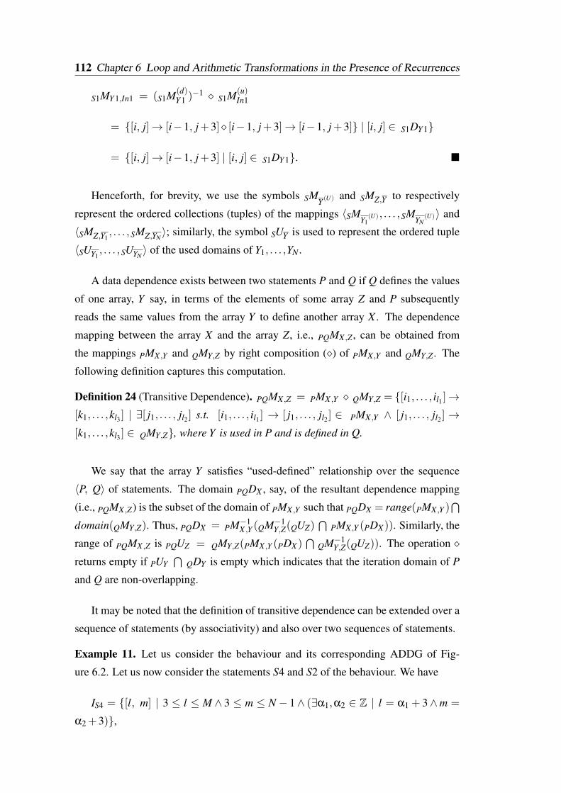
112 Chapter 6 Loop and Arithmetic Transformations in the Presence of Recurrences
S1MY 1,In1 = (S1M(d)Y 1 )
−1 S1M(u)In1
= [i, j]→ [i−1, j+3] [i−1, j+3]→ [i−1, j+3] | [i, j] ∈ S1DY 1
= [i, j]→ [i−1, j+3] | [i, j] ∈ S1DY 1.
Henceforth, for brevity, we use the symbols SMY (U) and SMZ,Y to respectively
represent the ordered collections (tuples) of the mappings 〈SMY1
(U), . . . ,SMYN
(U)〉 and
〈SMZ,Y1, . . . ,SMZ,YN
〉; similarly, the symbol SUY is used to represent the ordered tuple
〈SUY1, . . . ,SUYN
〉 of the used domains of Y1, . . . ,YN .
A data dependence exists between two statements P and Q if Q defines the values
of one array, Y say, in terms of the elements of some array Z and P subsequently
reads the same values from the array Y to define another array X . The dependence
mapping between the array X and the array Z, i.e., PQMX ,Z , can be obtained from
the mappings PMX ,Y and QMY,Z by right composition () of PMX ,Y and QMY,Z . The
following definition captures this computation.
Definition 24 (Transitive Dependence). PQMX ,Z = PMX ,Y QMY,Z = [i1, . . . , il1 ]→[k1, . . . ,kl3] | ∃[ j1, . . . , jl2 ] s.t. [i1, . . . , il1] → [ j1, . . . , jl2] ∈ PMX ,Y ∧ [ j1, . . . , jl2] →[k1, . . . ,kl3] ∈ QMY,Z, where Y is used in P and is defined in Q.
We say that the array Y satisfies “used-defined” relationship over the sequence
〈P, Q〉 of statements. The domain PQDX , say, of the resultant dependence mapping
(i.e., PQMX ,Z) is the subset of the domain of PMX ,Y such that PQDX = range(PMX ,Y )⋂
domain(QMY,Z). Thus, PQDX = PM−1X ,Y (QM−1
Y,Z(QUZ)⋂
PMX ,Y (PDX)). Similarly, the
range of PQMX ,Z is PQUZ = QMY,Z(PMX ,Y (PDX)⋂
QM−1Y,Z(QUZ)). The operation
returns empty if PUY⋂
QDY is empty which indicates that the iteration domain of P
and Q are non-overlapping.
It may be noted that the definition of transitive dependence can be extended over a
sequence of statements (by associativity) and also over two sequences of statements.
Example 11. Let us consider the behaviour and its corresponding ADDG of Fig-
ure 6.2. Let us now consider the statements S4 and S2 of the behaviour. We have
IS4 = [l, m] | 3 ≤ l ≤ M ∧ 3 ≤ m ≤ N − 1∧ (∃α1,α2 ∈ Z | l = α1 + 3∧m =
α2 +3),
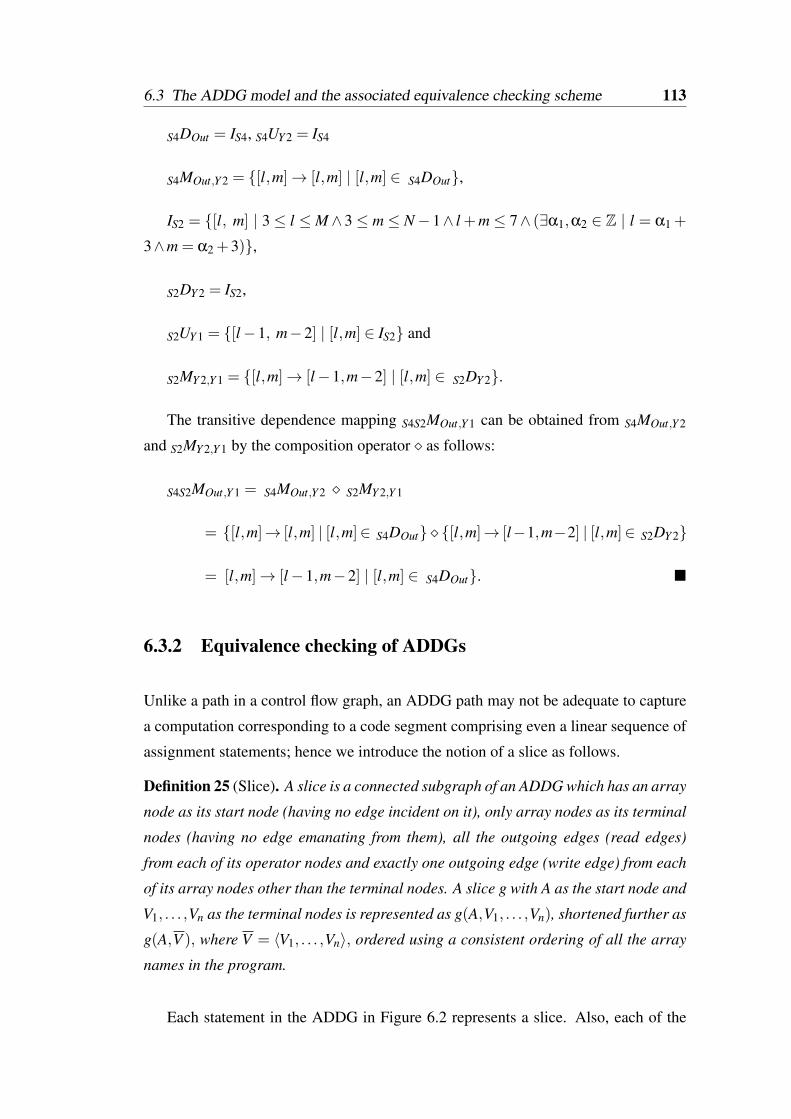
6.3 The ADDG model and the associated equivalence checking scheme 113
S4DOut = IS4, S4UY 2 = IS4
S4MOut,Y 2 = [l,m]→ [l,m] | [l,m] ∈ S4DOut,
IS2 = [l, m] | 3 ≤ l ≤M∧ 3 ≤ m ≤ N−1∧ l +m ≤ 7∧ (∃α1,α2 ∈ Z | l = α1 +
3∧m = α2 +3),
S2DY 2 = IS2,
S2UY 1 = [l−1, m−2] | [l,m] ∈ IS2 and
S2MY 2,Y 1 = [l,m]→ [l−1,m−2] | [l,m] ∈ S2DY 2.
The transitive dependence mapping S4S2MOut,Y 1 can be obtained from S4MOut,Y 2
and S2MY 2,Y 1 by the composition operator as follows:
S4S2MOut,Y 1 = S4MOut,Y 2 S2MY 2,Y 1
= [l,m]→ [l,m] | [l,m]∈ S4DOut [l,m]→ [l−1,m−2] | [l,m]∈ S2DY 2
= [l,m]→ [l−1,m−2] | [l,m] ∈ S4DOut.
6.3.2 Equivalence checking of ADDGs
Unlike a path in a control flow graph, an ADDG path may not be adequate to capture
a computation corresponding to a code segment comprising even a linear sequence of
assignment statements; hence we introduce the notion of a slice as follows.
Definition 25 (Slice). A slice is a connected subgraph of an ADDG which has an array
node as its start node (having no edge incident on it), only array nodes as its terminal
nodes (having no edge emanating from them), all the outgoing edges (read edges)
from each of its operator nodes and exactly one outgoing edge (write edge) from each
of its array nodes other than the terminal nodes. A slice g with A as the start node and
V1, . . . ,Vn as the terminal nodes is represented as g(A,V1, . . . ,Vn), shortened further as
g(A,V ), where V = 〈V1, . . . ,Vn〉, ordered using a consistent ordering of all the array
names in the program.
Each statement in the ADDG in Figure 6.2 represents a slice. Also, each of the
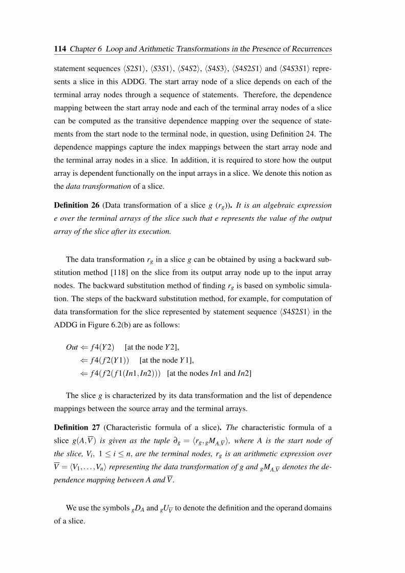
114 Chapter 6 Loop and Arithmetic Transformations in the Presence of Recurrences
statement sequences 〈S2S1〉, 〈S3S1〉, 〈S4S2〉, 〈S4S3〉, 〈S4S2S1〉 and 〈S4S3S1〉 repre-
sents a slice in this ADDG. The start array node of a slice depends on each of the
terminal array nodes through a sequence of statements. Therefore, the dependence
mapping between the start array node and each of the terminal array nodes of a slice
can be computed as the transitive dependence mapping over the sequence of state-
ments from the start node to the terminal node, in question, using Definition 24. The
dependence mappings capture the index mappings between the start array node and
the terminal array nodes in a slice. In addition, it is required to store how the output
array is dependent functionally on the input arrays in a slice. We denote this notion as
the data transformation of a slice.
Definition 26 (Data transformation of a slice g (rg)). It is an algebraic expression
e over the terminal arrays of the slice such that e represents the value of the output
array of the slice after its execution.
The data transformation rg in a slice g can be obtained by using a backward sub-
stitution method [118] on the slice from its output array node up to the input array
nodes. The backward substitution method of finding rg is based on symbolic simula-
tion. The steps of the backward substitution method, for example, for computation of
data transformation for the slice represented by statement sequence 〈S4S2S1〉 in the
ADDG in Figure 6.2(b) are as follows:
Out⇐ f 4(Y 2) [at the node Y 2],
⇐ f 4( f 2(Y 1)) [at the node Y 1],
⇐ f 4( f 2( f 1(In1, In2))) [at the nodes In1 and In2]
The slice g is characterized by its data transformation and the list of dependence
mappings between the source array and the terminal arrays.
Definition 27 (Characteristic formula of a slice). The characteristic formula of a
slice g(A,V ) is given as the tuple ∂g = 〈rg,gMA,V 〉, where A is the start node of
the slice, Vi, 1 ≤ i ≤ n, are the terminal nodes, rg is an arithmetic expression over
V = 〈V1, . . . ,Vn〉 representing the data transformation of g and gMA,V denotes the de-
pendence mapping between A and V .
We use the symbols gDA and gUV to denote the definition and the operand domains
of a slice.
6.3 The ADDG model and the associated equivalence checking scheme 115
Definition 28 (IO-slice). A slice is said to be an IO-slice iff its start node is an output
array node and all the terminal nodes are input array nodes.
It is required to capture the dependence of each output array on the input arrays.
Therefore, IO-slices are of interest to us. It may be noted that the slices represented
by the statement sequences 〈S4S2S1〉 and 〈S4S3S1〉 are the only two IO-slices in the
ADDG in Figure 6.2(b). To compute the characteristic formula of a slice, the nor-
malization technique for arithmetic expressions described in [141] is used along with
some simplification rules introduced in [86, 88].
Let G1 be the ADDG corresponding to an input behaviour and G2 be the ADDG
corresponding to the transformed behaviour obtained from the input behaviour through
loop and arithmetic transformations.
Definition 29 (Matching IO-slices). Two IO-slices g1 and g2 of an ADDG are said
to be matching, denoted as g1 ≈ g2, if the data transformations of both the slices are
equivalent.
Let the characteristic formula of gi(A,V ), i = 1,2, be 〈rgi, giMA,V 〉, where A is
an output array and V = 〈V1, . . . ,Vl〉 comprises input arrays. These two slices are
matching slices if rg1 ' rg2 . Due to single assignment form of the behaviour, the
domain of the dependence mapping between the output array A and the input array Vj
in V in the slices g1 and g2, however, are non-overlapping.
Definition 30 (IO-slice class). An IO-slice class is a maximum set of matching IO-
slices.
Let a slice class be Cg(A,V ) = g1, . . . ,gk. Let the characteristic formula of the
member slice gi, 1≤ i≤ k, be 〈rgi,giMA,V 〉. Due to single assignment form of the be-
haviour, the domain of the dependence mappings giMA,V j , for all i, 1≤ i≤ k, between
the output array A and the input array Vj in V , 1 ≤ j ≤ l, in the slices of Cg must be
non-overlapping. The domain of the dependence mapping CgMA,V j from A to Vj over
the entire class Cg is the union of the domains of giMA,V j , 1≤ i≤ k. So, the character-
istic formula of the slice class Cg is 〈rCg,CgMA,V 〉, where rCg is the data transformation
of any of the slices in Cg and CgMA,V j , 1≤ j ≤ l, in CgMA,V is
CgMA,V j =⋃
1≤i≤kgiMA,V j .
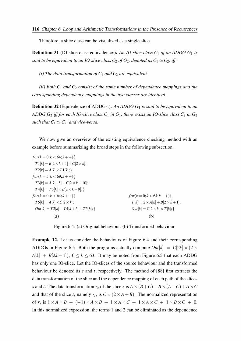
116 Chapter 6 Loop and Arithmetic Transformations in the Presence of Recurrences
Therefore, a slice class can be visualized as a single slice.
Definition 31 (IO-slice class equivalence:). An IO-slice class C1 of an ADDG G1 is
said to be equivalent to an IO-slice class C2 of G2, denoted as C1 'C2, iff
(i) The data transformation of C1 and C2 are equivalent.
(ii) Both C1 and C2 consist of the same number of dependence mappings and the
corresponding dependence mappings in the two classes are identical.
Definition 32 (Equivalence of ADDGs:). An ADDG G1 is said to be equivalent to an
ADDG G2 iff for each IO-slice class C1 in G1, there exists an IO-slice class C2 in G2
such that C1 'C2, and vice-versa.
We now give an overview of the existing equivalence checking method with an
example before summarizing the broad steps in the following subsection.
f or(k = 0;k < 64;k++)T 1[k] = B[2× k+1]+C[2× k];
T 2[k] = A[k]×T 1[k];f or(k = 5;k < 69;k++)
T 3[k] = A[k−5]−C[2× k−10];
T 4[k] = T 3[k]×B[2× k−9];f or(k = 0;k < 64;k++)
T 5[k] = A[k]×C[2× k];
Out[k] = T 2[k]−T 4[k+5]+T 5[k];
(a)
f or(k = 0;k < 64;k++)T [k] = 2×A[k]+B[2× k+1];
Out[k] =C[2× k]×T [k];
(b)
Figure 6.4: (a) Original behaviour. (b) Transformed behaviour.
Example 12. Let us consider the behaviours of Figure 6.4 and their corresponding
ADDGs in Figure 6.5. Both the programs actually compute Out[k] = C[2k]× (2×A[k] + B[2k+ 1]), 0 ≤ k ≤ 63. It may be noted from Figure 6.5 that each ADDG
has only one IO-slice. Let the IO-slices of the source behaviour and the transformed
behaviour be denoted as s and t, respectively. The method of [88] first extracts the
data transformation of the slice and the dependence mapping of each path of the slices
s and t. The data transformation rs of the slice s is A× (B+C)−B× (A−C)+A×C
and that of the slice t, namely rt , is C× (2×A+B). The normalized representation
of rs is 1×A×B + (−1)×A×B + 1×A×C + 1×A×C + 1×B×C + 0.
In this normalized expression, the terms 1 and 2 can be eliminated as the dependence
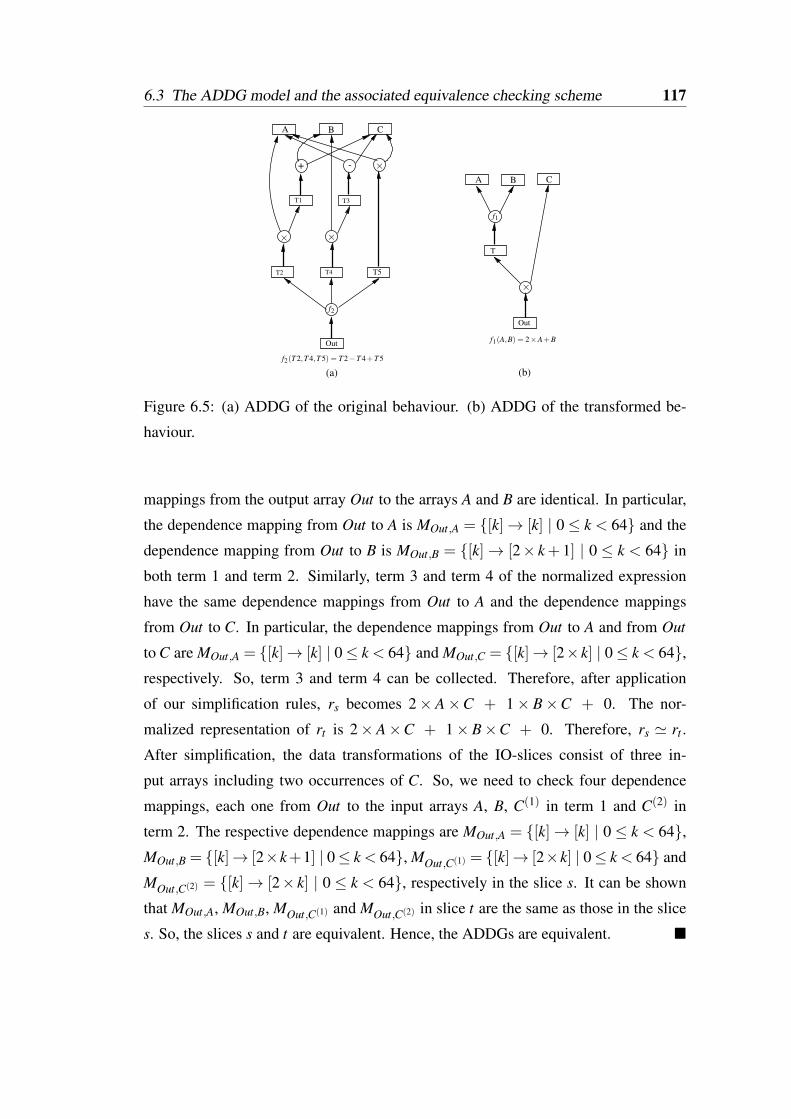
6.3 The ADDG model and the associated equivalence checking scheme 117
-
A
× ×
×+
(a)
f2
(b)
A
Out
×
f1
f1(A,B) = 2×A+B
B
f2(T 2,T 4,T 5) = T 2−T 4+T 5
T5T4T2
T3T1
C
T
Out
B C
Figure 6.5: (a) ADDG of the original behaviour. (b) ADDG of the transformed be-
haviour.
mappings from the output array Out to the arrays A and B are identical. In particular,
the dependence mapping from Out to A is MOut,A = [k]→ [k] | 0 ≤ k < 64 and the
dependence mapping from Out to B is MOut,B = [k]→ [2× k+ 1] | 0 ≤ k < 64 in
both term 1 and term 2. Similarly, term 3 and term 4 of the normalized expression
have the same dependence mappings from Out to A and the dependence mappings
from Out to C. In particular, the dependence mappings from Out to A and from Out
to C are MOut,A = [k]→ [k] | 0≤ k < 64 and MOut,C = [k]→ [2×k] | 0≤ k < 64,respectively. So, term 3 and term 4 can be collected. Therefore, after application
of our simplification rules, rs becomes 2× A×C + 1× B×C + 0. The nor-
malized representation of rt is 2× A×C + 1× B×C + 0. Therefore, rs ' rt .
After simplification, the data transformations of the IO-slices consist of three in-
put arrays including two occurrences of C. So, we need to check four dependence
mappings, each one from Out to the input arrays A, B, C(1) in term 1 and C(2) in
term 2. The respective dependence mappings are MOut,A = [k]→ [k] | 0 ≤ k < 64,MOut,B = [k]→ [2×k+1] | 0≤ k < 64, MOut,C(1) = [k]→ [2×k] | 0≤ k < 64 and
MOut,C(2) = [k]→ [2× k] | 0 ≤ k < 64, respectively in the slice s. It can be shown
that MOut,A, MOut,B, MOut,C(1) and MOut,C(2) in slice t are the same as those in the slice
s. So, the slices s and t are equivalent. Hence, the ADDGs are equivalent.
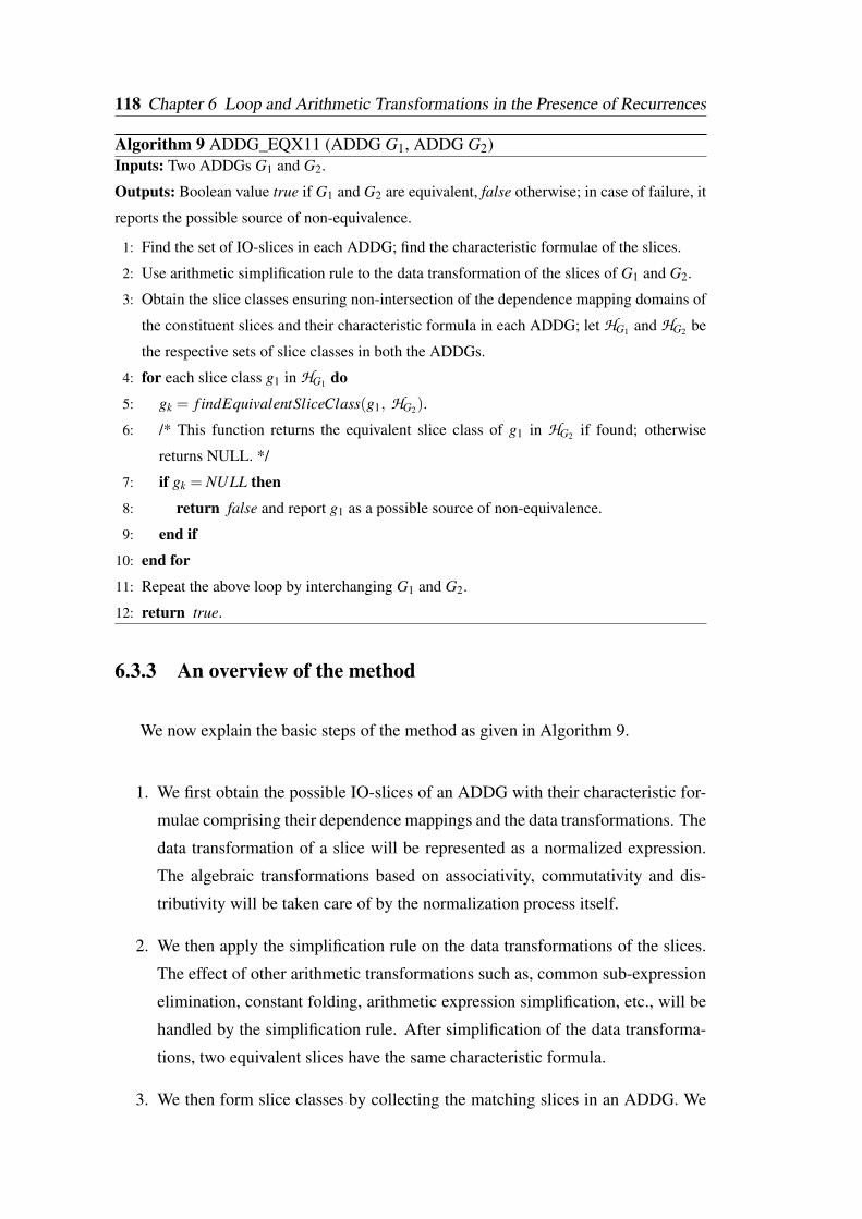
118 Chapter 6 Loop and Arithmetic Transformations in the Presence of Recurrences
Algorithm 9 ADDG_EQX11 (ADDG G1, ADDG G2)Inputs: Two ADDGs G1 and G2.
Outputs: Boolean value true if G1 and G2 are equivalent, false otherwise; in case of failure, it
reports the possible source of non-equivalence.
1: Find the set of IO-slices in each ADDG; find the characteristic formulae of the slices.
2: Use arithmetic simplification rule to the data transformation of the slices of G1 and G2.
3: Obtain the slice classes ensuring non-intersection of the dependence mapping domains of
the constituent slices and their characteristic formula in each ADDG; let HG1 and HG2 be
the respective sets of slice classes in both the ADDGs.
4: for each slice class g1 in HG1 do
5: gk = f indEquivalentSliceClass(g1, HG2).
6: /* This function returns the equivalent slice class of g1 in HG2 if found; otherwise
returns NULL. */
7: if gk = NULL then
8: return false and report g1 as a possible source of non-equivalence.
9: end if
10: end for
11: Repeat the above loop by interchanging G1 and G2.
12: return true.
6.3.3 An overview of the method
We now explain the basic steps of the method as given in Algorithm 9.
1. We first obtain the possible IO-slices of an ADDG with their characteristic for-
mulae comprising their dependence mappings and the data transformations. The
data transformation of a slice will be represented as a normalized expression.
The algebraic transformations based on associativity, commutativity and dis-
tributivity will be taken care of by the normalization process itself.
2. We then apply the simplification rule on the data transformations of the slices.
The effect of other arithmetic transformations such as, common sub-expression
elimination, constant folding, arithmetic expression simplification, etc., will be
handled by the simplification rule. After simplification of the data transforma-
tions, two equivalent slices have the same characteristic formula.
3. We then form slice classes by collecting the matching slices in an ADDG. We
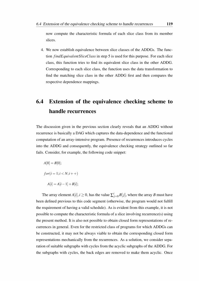
6.4 Extension of the equivalence checking scheme to handle recurrences 119
now compute the characteristic formula of each slice class from its member
slices.
4. We now establish equivalence between slice classes of the ADDGs. The func-
tion f indEquivalentSliceClass in step 5 is used for this purpose. For each slice
class, this function tries to find its equivalent slice class in the other ADDG.
Corresponding to each slice class, the function uses the data transformation to
find the matching slice class in the other ADDG first and then compares the
respective dependence mappings.
6.4 Extension of the equivalence checking scheme to
handle recurrences
The discussion given in the previous section clearly reveals that an ADDG without
recurrence is basically a DAG which captures the data-dependence and the functional
computation of an array-intensive program. Presence of recurrences introduces cycles
into the ADDG and consequently, the equivalence checking strategy outlined so far
fails. Consider, for example, the following code snippet:
A[0] = B[0];
f or(i = 1; i < N; i++)
A[i] = A[i−1]+B[i];
The array element A[i], i≥ 0, has the value ∑ij=0 B[ j], where the array B must have
been defined previous to this code segment (otherwise, the program would not fulfill
the requirement of having a valid schedule). As is evident from this example, it is not
possible to compute the characteristic formula of a slice involving recurrence(s) using
the present method. It is also not possible to obtain closed form representations of re-
currences in general. Even for the restricted class of programs for which ADDGs can
be constructed, it may not be always viable to obtain the corresponding closed form
representations mechanically from the recurrences. As a solution, we consider sepa-
ration of suitable subgraphs with cycles from the acyclic subgraphs of the ADDG. For
the subgraphs with cycles, the back edges are removed to make them acyclic. Once
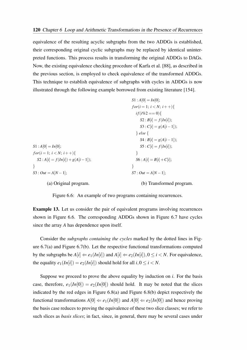
120 Chapter 6 Loop and Arithmetic Transformations in the Presence of Recurrences
equivalence of the resulting acyclic subgraphs from the two ADDGs is established,
their corresponding original cyclic subgraphs may be replaced by identical uninter-
preted functions. This process results in transforming the original ADDGs to DAGs.
Now, the existing equivalence checking procedure of Karfa et al. [88], as described in
the previous section, is employed to check equivalence of the transformed ADDGs.
This technique to establish equivalence of subgraphs with cycles in ADDGs is now
illustrated through the following example borrowed from existing literature [154].
S1 : A[0] = In[0];
f or(i = 1; i < N; i++)S2 : A[i] = f (In[i])+g(A[i−1]);
S3 : Out = A[N−1];
(a) Original program.
S1 : A[0] = In[0];
f or(i = 1; i < N; i++)i f (i%2 == 0)
S2 : B[i] = f (In[i]);
S3 : C[i] = g(A[i−1]);
else S4 : B[i] = g(A[i−1]);
S5 : C[i] = f (In[i]);
S6 : A[i] = B[i]+C[i];
S7 : Out = A[N−1];
(b) Transformed program.
Figure 6.6: An example of two programs containing recurrences.
Example 13. Let us consider the pair of equivalent programs involving recurrences
shown in Figure 6.6. The corresponding ADDGs shown in Figure 6.7 have cycles
since the array A has dependence upon itself.
Consider the subgraphs containing the cycles marked by the dotted lines in Fig-
ure 6.7(a) and Figure 6.7(b). Let the respective functional transformations computed
by the subgraphs be A[i]⇐ e1(In[i]) and A[i]⇐ e2(In[i]),0≤ i < N. For equivalence,
the equality e1(In[i]) = e2(In[i]) should hold for all i,0≤ i < N.
Suppose we proceed to prove the above equality by induction on i. For the basis
case, therefore, e1(In[0]) = e2(In[0]) should hold. It may be noted that the slices
indicated by the red edges in Figure 6.8(a) and Figure 6.8(b) depict respectively the
functional transformations A[0]⇐ e1(In[0]) and A[0]⇐ e2(In[0]) and hence proving
the basis case reduces to proving the equivalence of these two slice classes; we refer to
such slices as basis slices; in fact, since, in general, there may be several cases under
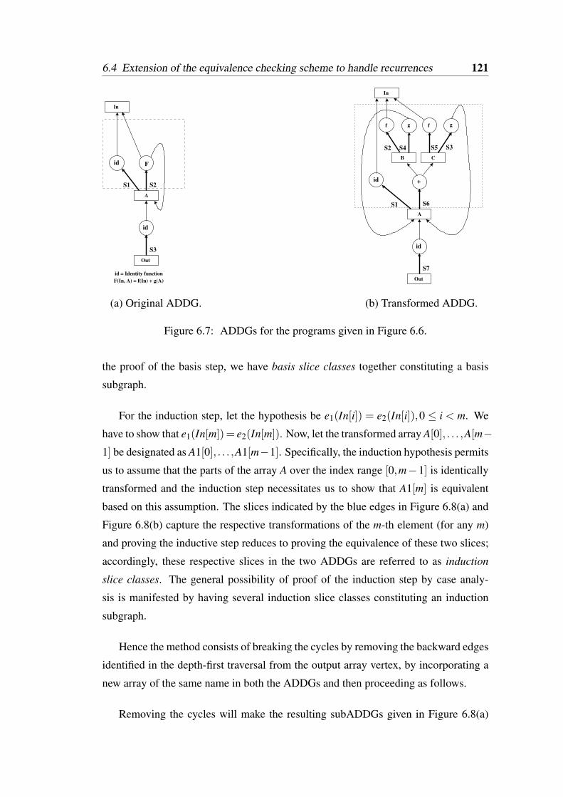
6.4 Extension of the equivalence checking scheme to handle recurrences 121
S3
S2
Out
A
S1
In
id = Identity functionF(In, A) = f(In) + g(A)
Fid
id
(a) Original ADDG.
S7
S6
Out
A
B C
In
f fg g
S1
S2 S4 S5 S3
+
id
id
(b) Transformed ADDG.
Figure 6.7: ADDGs for the programs given in Figure 6.6.
the proof of the basis step, we have basis slice classes together constituting a basis
subgraph.
For the induction step, let the hypothesis be e1(In[i]) = e2(In[i]),0 ≤ i < m. We
have to show that e1(In[m])= e2(In[m]). Now, let the transformed array A[0], . . . ,A[m−1] be designated as A1[0], . . . ,A1[m−1]. Specifically, the induction hypothesis permits
us to assume that the parts of the array A over the index range [0,m−1] is identically
transformed and the induction step necessitates us to show that A1[m] is equivalent
based on this assumption. The slices indicated by the blue edges in Figure 6.8(a) and
Figure 6.8(b) capture the respective transformations of the m-th element (for any m)
and proving the inductive step reduces to proving the equivalence of these two slices;
accordingly, these respective slices in the two ADDGs are referred to as induction
slice classes. The general possibility of proof of the induction step by case analy-
sis is manifested by having several induction slice classes constituting an induction
subgraph.
Hence the method consists of breaking the cycles by removing the backward edges
identified in the depth-first traversal from the output array vertex, by incorporating a
new array of the same name in both the ADDGs and then proceeding as follows.
Removing the cycles will make the resulting subADDGs given in Figure 6.8(a)
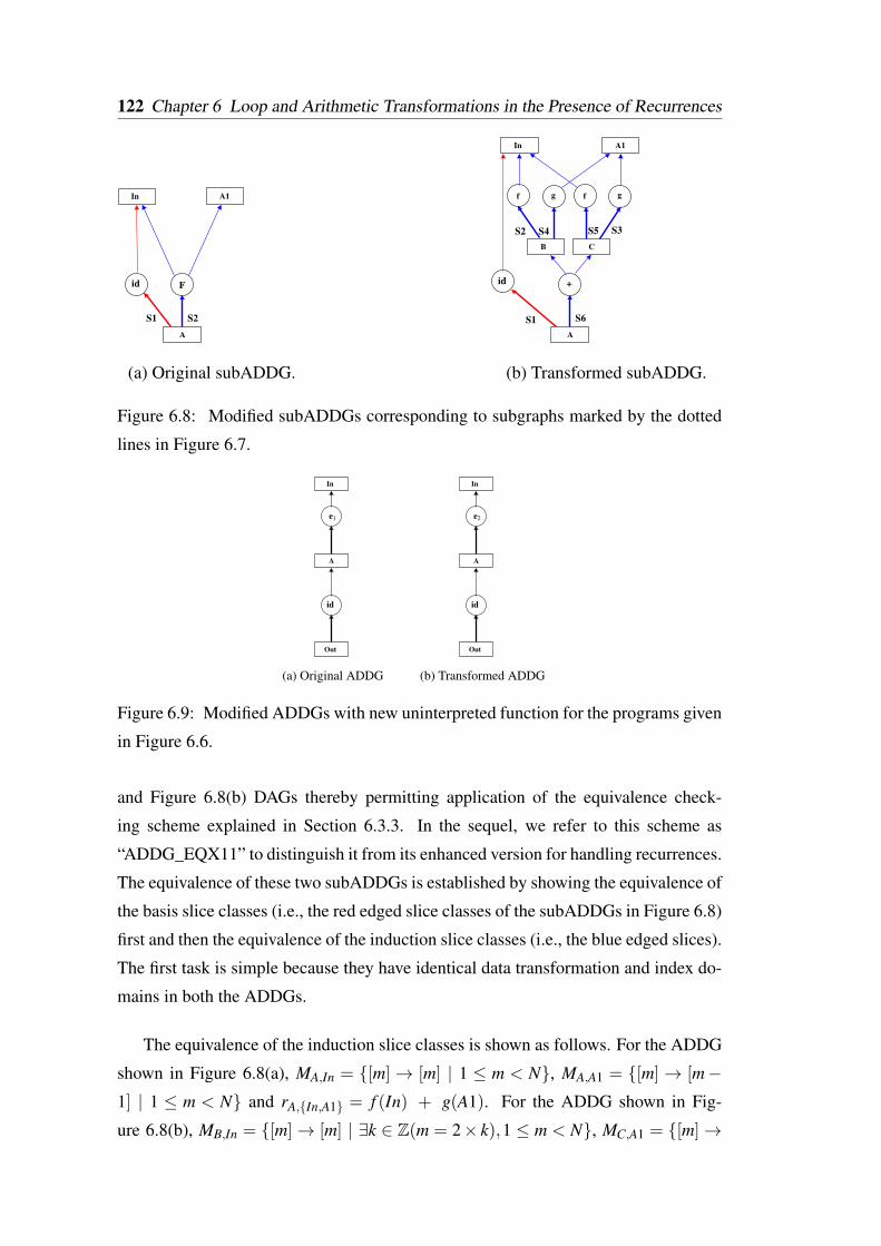
122 Chapter 6 Loop and Arithmetic Transformations in the Presence of Recurrences
S2A
S1
In A1
Fid
(a) Original subADDG.
S6A
B C
In A1
f fg g
S1
S2 S4 S5 S3
+id
(b) Transformed subADDG.
Figure 6.8: Modified subADDGs corresponding to subgraphs marked by the dotted
lines in Figure 6.7.
Out
A
e1
In
Out
A
e2
In
(a) Original ADDG (b) Transformed ADDG
idid
Figure 6.9: Modified ADDGs with new uninterpreted function for the programs given
in Figure 6.6.
and Figure 6.8(b) DAGs thereby permitting application of the equivalence check-
ing scheme explained in Section 6.3.3. In the sequel, we refer to this scheme as
“ADDG_EQX11” to distinguish it from its enhanced version for handling recurrences.
The equivalence of these two subADDGs is established by showing the equivalence of
the basis slice classes (i.e., the red edged slice classes of the subADDGs in Figure 6.8)
first and then the equivalence of the induction slice classes (i.e., the blue edged slices).
The first task is simple because they have identical data transformation and index do-
mains in both the ADDGs.
The equivalence of the induction slice classes is shown as follows. For the ADDG
shown in Figure 6.8(a), MA,In = [m]→ [m] | 1 ≤ m < N, MA,A1 = [m]→ [m−1] | 1 ≤ m < N and rA,In,A1 = f (In) + g(A1). For the ADDG shown in Fig-
ure 6.8(b), MB,In = [m]→ [m] | ∃k ∈ Z(m = 2× k),1 ≤ m < N, MC,A1 = [m]→
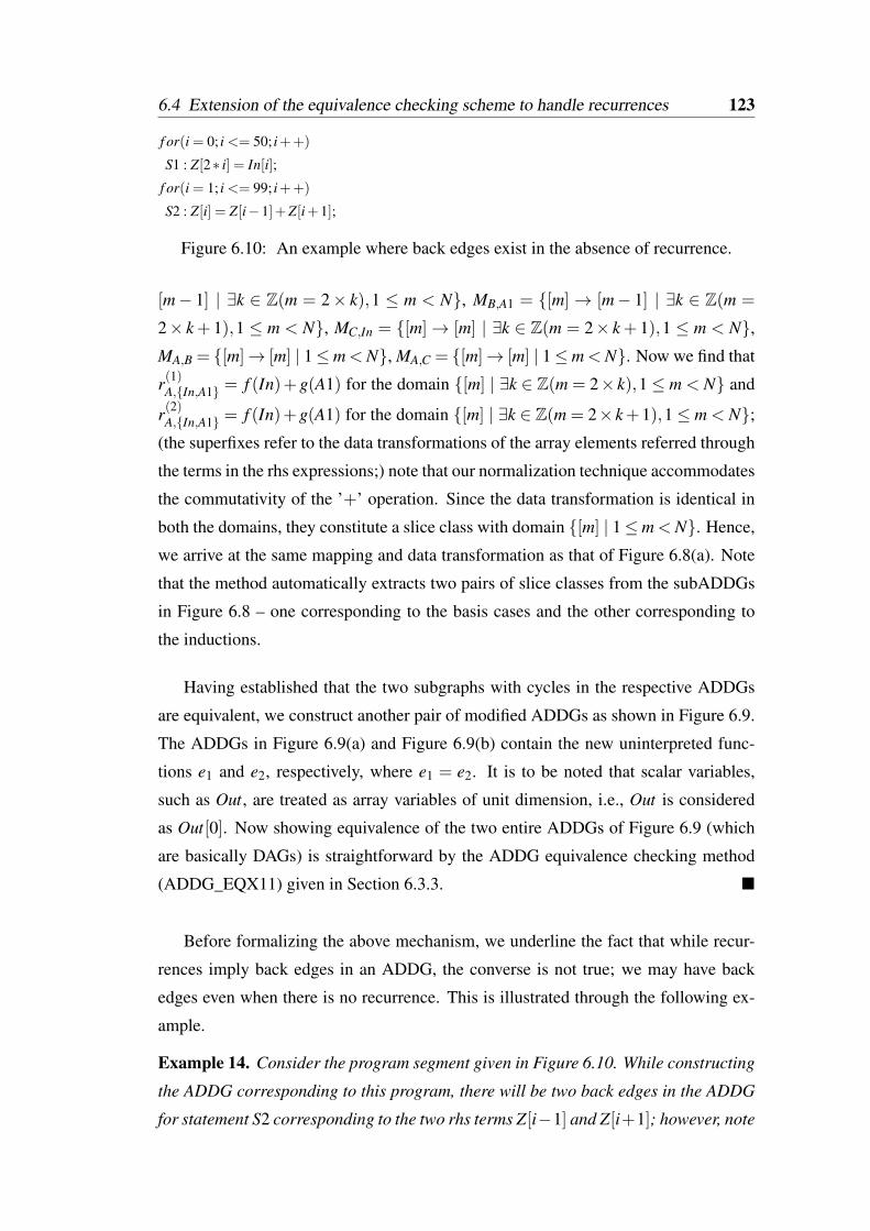
6.4 Extension of the equivalence checking scheme to handle recurrences 123
f or(i = 0; i <= 50; i++)
S1 : Z[2∗ i] = In[i];
f or(i = 1; i <= 99; i++)
S2 : Z[i] = Z[i−1]+Z[i+1];
Figure 6.10: An example where back edges exist in the absence of recurrence.
[m− 1] | ∃k ∈ Z(m = 2× k),1 ≤ m < N, MB,A1 = [m]→ [m− 1] | ∃k ∈ Z(m =
2× k+ 1),1 ≤ m < N, MC,In = [m]→ [m] | ∃k ∈ Z(m = 2× k+ 1),1 ≤ m < N,MA,B = [m]→ [m] | 1≤m < N, MA,C = [m]→ [m] | 1≤m < N. Now we find that
r(1)A,In,A1 = f (In)+g(A1) for the domain [m] | ∃k ∈ Z(m = 2× k),1≤ m < N and
r(2)A,In,A1 = f (In)+g(A1) for the domain [m] | ∃k ∈ Z(m = 2× k+1),1≤ m < N;(the superfixes refer to the data transformations of the array elements referred through
the terms in the rhs expressions;) note that our normalization technique accommodates
the commutativity of the ’+’ operation. Since the data transformation is identical in
both the domains, they constitute a slice class with domain [m] | 1≤m < N. Hence,
we arrive at the same mapping and data transformation as that of Figure 6.8(a). Note
that the method automatically extracts two pairs of slice classes from the subADDGs
in Figure 6.8 – one corresponding to the basis cases and the other corresponding to
the inductions.
Having established that the two subgraphs with cycles in the respective ADDGs
are equivalent, we construct another pair of modified ADDGs as shown in Figure 6.9.
The ADDGs in Figure 6.9(a) and Figure 6.9(b) contain the new uninterpreted func-
tions e1 and e2, respectively, where e1 = e2. It is to be noted that scalar variables,
such as Out, are treated as array variables of unit dimension, i.e., Out is considered
as Out[0]. Now showing equivalence of the two entire ADDGs of Figure 6.9 (which
are basically DAGs) is straightforward by the ADDG equivalence checking method
(ADDG_EQX11) given in Section 6.3.3.
Before formalizing the above mechanism, we underline the fact that while recur-
rences imply back edges in an ADDG, the converse is not true; we may have back
edges even when there is no recurrence. This is illustrated through the following ex-
ample.
Example 14. Consider the program segment given in Figure 6.10. While constructing
the ADDG corresponding to this program, there will be two back edges in the ADDG
for statement S2 corresponding to the two rhs terms Z[i−1] and Z[i+1]; however, note
124 Chapter 6 Loop and Arithmetic Transformations in the Presence of Recurrences
that statement S2 does not have any data dependency on itself since the whole of its
operand domain has already been defined in statement S1. These cases can be handled
within the framework of the equivalence checking method described in Section 6.3.3
by permitting computation of transitive dependence through the cycles only once and
then continuing through the other edges emanating from the array vertex Z.
Example 14 leads us to the following definition.
Definition 33 (Recurrence Array Vertex). An array vertex Z which is identified as the
destination of a back edge (of a cycle c) during a depth-first traversal of an ADDG
starting from an output array such that cDZ⋂
cUZ 6= /0 is called a recurrence array
vertex.
Let us first elaborate what the above definition entails. Obviously, recurrences lead
to cycles and a back edge basically identifies the source of the recurrence namely, the
array Z which has been defined in terms of itself. Let the statement leading to the
recurrence in some program be
S : Z[l] = f (Y [r0],Z[r1],Z[r2],Z[r3]);
Let the symbol Z(i) represent the i-th occurrence of Z in the rhs of S. For Z to qual-
ify as a recurrence array vertex, (SM(d)Z,Z(1)(IS) = SDZ)
⋂(SM(u)
Z,Z(1)(IS) = SUZ(1)) 6= /0 or
SDZ⋂
SUZ(2) 6= /0 or SDZ⋂
SUZ(3) 6= /0 should hold (other arrays such as, Y , do not par-
ticipate in this procedure). In case the recurrence occurs through a cycle c involving
multiple statements, we shall have to consider the transitive dependences over c. This
check for overlapping definition and operand domains helps in segregating cases of
true recurrences from those as shown in Example 14.
As indicated in Example 13, for each recurrence array vertex, we need to find a
minimum subgraph with cycle(s) so that the computed values of the recurrence array
elements can be captured by an uninterpreted function with proper arguments. Finding
such minimum subgraphs with cycles in an ADDG involves prior identification of
strongly connected components (SCCs) in the ADDG.
Definition 34 (Basis Subgraph B(Z,Y i1, . . . ,Y
iki,ki ≥ 1,1≤ i≤m) for the recurrence
array vertex Z). Let C (Z) be an SCC in the ADDG having Z as the recurrence ar-
ray vertex. Let ei = 〈Z, fi〉,1 ≤ i ≤ m, be m write edges which are not contained
in C (Z); also, let 〈 fi,Y i1〉, . . . ,〈 fi,Y i
ki〉,ki ≥ 1, be all the existing read edges emanat-
ing from the operator vertex fi in the ADDG. The subgraph B(Z,Y i1, . . . ,Y
iki,ki ≥

6.4 Extension of the equivalence checking scheme to handle recurrences 125
1,1 ≤ i ≤ m) containing the array vertex Z, all such operator vertices fi,1 ≤ i ≤m, and the corresponding array vertices Y i
1, . . . ,Yiki
along with the connecting edges
〈Z, fi〉,〈 fi,Y i1〉, . . . ,〈 fi,Y i
ki〉 is called a basis subgraph. For brevity, we represent such a
basis subgraph as B(Z,Y ), where Y represents the set Y i1, . . . ,Y
iki,ki ≥ 1,1 ≤ i ≤ m
ordered using a consistent ordering of all the array names used in the program.
Note that the subgraph B(Z,Y ) is the minimum subgraph that encompasses the
basis step(s) of a recurrence involving the recurrence array Z in the program. The
arrays Y ij ,1 ≤ j ≤ ki,1 ≤ i ≤ m, in Y need not be all distinct. If there are multiple
basis steps with different data transformations, then there will be multiple basis slice
classes; it is to be noted that all such basis slice classes are collectively covered in
B(Z,Y ).
Definition 35 (Induction Subgraph D(Z,T i1, . . . ,T
iki,ki ≥ 1,1≤ i≤m, W i
1, . . . ,Wiki,
ki ≥ 1,1 ≤ i ≤ n) for the recurrence array vertex Z). Let C (Z) be an SCC in the
ADDG having Z as the recurrence vertex.
1) Let ei = 〈Xi,hi〉,1 ≤ i ≤ m, be m write edges where Xi(6= Z) is an array vertex in
C (Z) such that ei is not contained in C (Z); also, let 〈hi,T i1〉, . . . ,〈hi,T i
ki〉,ki≥ 1,1≤ i≤
m, be all the existing read edges emanating from the operator vertex hi in the ADDG.
Let the connected subgraph containing C (Z) along with the vertices hi,T i1, . . . ,T
iki,ki≥
1,1≤ i≤ m, be designated as D ′(Z,T i1, . . . ,T
iki,ki ≥ 1,1≤ i≤ m).
2) Let gi,1 ≤ i ≤ n, be n operator vertices in C (Z) such that there is a read edge e
emanating from gi which is not contained in C (Z); also, let 〈gi,W i1〉, . . . ,〈gi,W i
k′i〉,k′i ≥
1,1 ≤ i ≤ n, be all the existing read edges emanating from the operator vertex gi in
the ADDG which are not already covered in C (Z); the connected subgraph containing
D ′(Z,T i1, . . . ,T
iki,ki ≥ 1,1≤ i≤m) along with all such array vertices W i
1, . . . ,Wik′i,k′i ≥
1,1 ≤ i ≤ n, is called an induction subgraph and is represented as D(Z,V ), where
V is the set T i1, . . . ,T
iki,ki ≥ 1,1≤ i≤ m
⋃W i
1, . . . ,Wik′i,k′i ≥ 1,1≤ i≤ n) ordered
using a uniform ordering of all the array names used in the program.
Note that the subgraph D(Z,V ) is the minimum subgraph that encompasses the
induction step(s) of a recurrence involving the array Z in the program. Once the in-
duction subgraph is found, we do not need to distinguish between the arrays marked as
T ’s and W ’s; hence they are jointly denoted as V . The arrays T ij ,1≤ j≤ ki,1≤ i≤m,
and W ij ,1 ≤ j ≤ ki,1 ≤ i ≤ n, in V need not be all distinct. If there are multiple in-
duction steps with different data transformations, then there will be multiple induction
126 Chapter 6 Loop and Arithmetic Transformations in the Presence of Recurrences
slice classes; it is to be noted that all such induction slice classes are collectively cov-
ered in D(Z,V ).
Definition 36 (Recurrence Subgraph E(Z,Y ,V) for the basis subgraph B(Z,Y ) and
the induction subgraph D(Z,V )). The subgraph E(Z,Y ,V ) which is obtained by com-
bining a basis subgraph B(Z,Y ) and an induction subgraph D(Z,V ) having the same
recurrence array vertex Z in an ADDG is called a recurrence subgraph.
Note that the subgraph E(Z,Y ,V ) is the minimum subgraph that encompasses the
recurrence involving the array Z in the program.
Figure 6.11(a) shows a schema of a program involving a recurrence and Fig-
ure 6.11(b) shows its ADDG representation; note that we have shown a single back
edge from the operator vertices g1 and gp instead of m such back edges for clarity;
the corresponding basis subgraph and the induction subgraph have been given in Fig-
ure 6.12(a) and Figure 6.12(b), respectively.
In order to compare two recurrence subgraphs, E1(Z,Y1,V1) and E2(Z,Y2,V2),
say, from two different ADDGs, and represent them as uninterpreted functions sub-
sequently, the arguments Y and V must be identical, i.e., Y1 = Y2 and V1 = V2 have
to hold. In case they do not hold, we identify the uncommon arrays, i.e., arrays that
appear in only one of the ADDGs but not both, occurring in Yi and Vi, i ∈ 1,2;for each such array, T say, we identify the minimum subgraph GT (T,XT ), say (with
T as the start array vertex and XT as the terminal array vertices), where XT com-
prises only common arrays, i.e., arrays that appear in both the ADDGs. If T ∈ Yi
(Vi), then the basis subgraph Bi(Z,Yi) (induction subgraph Di(Z,Vi)) is extended by
including GT and treat the resulting subgraph as the basis subgraph (induction sub-
graph) for establishing equivalence of the two ADDGs. Algorithm 10 captures this
process, where the module “extendSubgraph” basically extends the passed recurrence
subgraph along each uncommon array vertex A by including all edges of the form
〈A, fi〉 and 〈 fi,Xi〉,1≤ i≤ p,; this process of extension is repeated for each uncommon
array vertex Xi,1 ≤ i ≤ p, until each of the terminal nodes of the extended subgraph
is a common array vertex.
For example, from Figure 6.7(b), we shall get an SCC C (A), say, comprising the
vertices (A, +, B, C, gS4, gS3) with A designated as the recurrence array vertex; the
corresponding basis subgraph B(A, In) comprises the vertices A, idS1, In and the
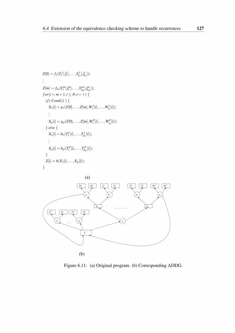
6.4 Extension of the equivalence checking scheme to handle recurrences 127
Z[0] = f1(Y 11 [ j
11], . . . ,Y
1k1[ j1
k1]);
...
Z[m] = fm(Y m1 [ jm
1 ], . . . ,Ymkm[ jm
km]);
f or(i = m+1, i≤ N; i++) i f ( Cond(i) )
X1[i] = g1(Z[0], . . . ,Z[m],W 11 [i], . . . ,W
1l1[i]);
...
Xp[i] = gp(Z[0], . . . ,Z[m],W p1 [i], . . . ,W
plp[i]);
else X1[i] = h1(T 1
1 [i], . . . ,T1
d1[i]);
...
Xp[i] = hp(Tp
1 [i], . . . ,T pdp[i]);
Z[i] = h(X1[i], . . . ,Xp[i]);
(a)
Z
Y 11 Y m
kmY m
1
f1 fm
Y 1k1
. . . .
. . . . . .
h1
. . .
hp
. . .
gp
. . .
g1
. . .
. . . . . . .
h
XpX1
W plp
W p1T p
dpT p
1T 1d1
T 11W 1
l1W 11
(b)
Figure 6.11: (a) Original program. (b) Corresponding ADDG.
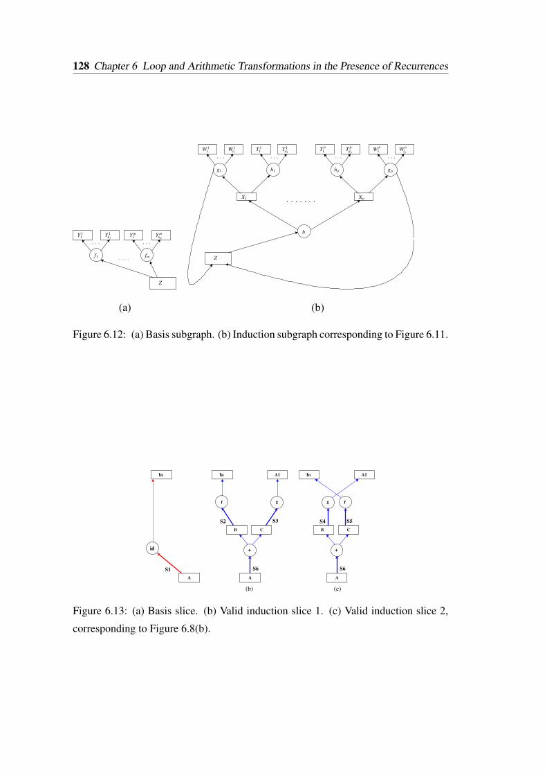
128 Chapter 6 Loop and Arithmetic Transformations in the Presence of Recurrences
Z
Y 11 Y m
kmY m
1
f1 fm
Y 1k1
. . . .
. . . . . .
(a)
Z
h1
. . .
hp
. . .
gp
. . .
g1
. . .
. . . . . . .
h
XpX1
W plp
W p1T p
dpT p
1T 1d1
T 11W 1
l1W 11
(b)
Figure 6.12: (a) Basis subgraph. (b) Induction subgraph corresponding to Figure 6.11.
S6A
B C
In A1
f g
S2 S3
+
S6A
B C
In A1
fg
S4 S5
+
A
In
S1
(b) (c)
id
Figure 6.13: (a) Basis slice. (b) Valid induction slice 1. (c) Valid induction slice 2,
corresponding to Figure 6.8(b).
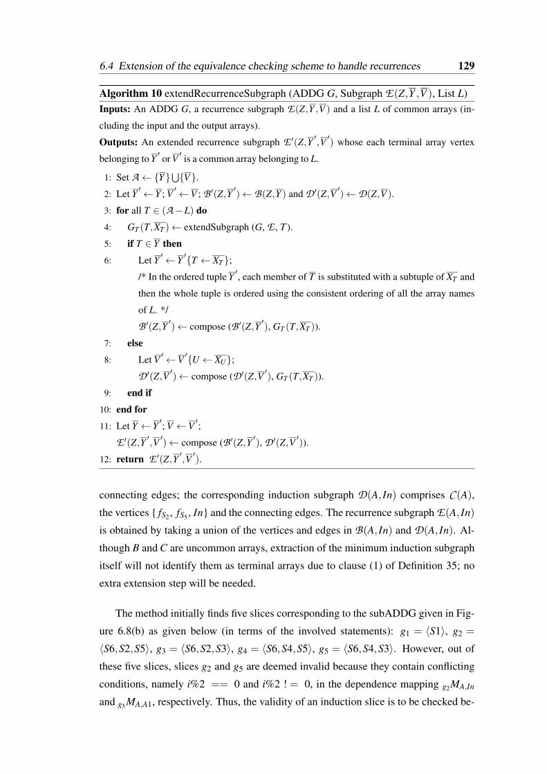
6.4 Extension of the equivalence checking scheme to handle recurrences 129
Algorithm 10 extendRecurrenceSubgraph (ADDG G, Subgraph E(Z,Y ,V ), List L)Inputs: An ADDG G, a recurrence subgraph E(Z,Y ,V ) and a list L of common arrays (in-
cluding the input and the output arrays).
Outputs: An extended recurrence subgraph E ′(Z,Y ′,V ′) whose each terminal array vertex
belonging to Y ′ or V ′ is a common array belonging to L.
1: Set A ←Y⋃V.
2: Let Y ′← Y ; V ′←V ; B ′(Z,Y ′)← B(Z,Y ) and D ′(Z,V ′)←D(Z,V ).
3: for all T ∈ (A−L) do
4: GT (T,XT )← extendSubgraph (G, E , T ).
5: if T ∈ Y then
6: Let Y ′← Y ′T ← XT;/* In the ordered tuple Y ′, each member of T is substituted with a subtuple of XT and
then the whole tuple is ordered using the consistent ordering of all the array names
of L. */
B ′(Z,Y ′)← compose (B ′(Z,Y ′), GT (T,XT )).
7: else
8: Let V ′←V ′U ← XU;D ′(Z,V ′)← compose (D ′(Z,V ′), GT (T,XT )).
9: end if
10: end for
11: Let Y ← Y ′; V ←V ′;
E ′(Z,Y ′,V ′)← compose (B ′(Z,Y ′), D ′(Z,V ′)).12: return E ′(Z,Y ′,V ′).
connecting edges; the corresponding induction subgraph D(A, In) comprises C (A),
the vertices fS2 , fS5 , In and the connecting edges. The recurrence subgraph E(A, In)
is obtained by taking a union of the vertices and edges in B(A, In) and D(A, In). Al-
though B and C are uncommon arrays, extraction of the minimum induction subgraph
itself will not identify them as terminal arrays due to clause (1) of Definition 35; no
extra extension step will be needed.
The method initially finds five slices corresponding to the subADDG given in Fig-
ure 6.8(b) as given below (in terms of the involved statements): g1 = 〈S1〉, g2 =
〈S6,S2,S5〉, g3 = 〈S6,S2,S3〉, g4 = 〈S6,S4,S5〉, g5 = 〈S6,S4,S3〉. However, out of
these five slices, slices g2 and g5 are deemed invalid because they contain conflicting
conditions, namely i%2 == 0 and i%2 ! = 0, in the dependence mapping g2MA,In
and g5MA,A1, respectively. Thus, the validity of an induction slice is to be checked be-
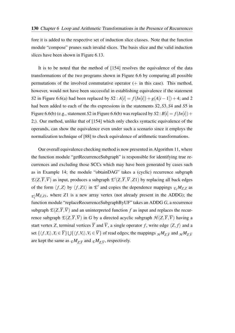
130 Chapter 6 Loop and Arithmetic Transformations in the Presence of Recurrences
fore it is added to the respective set of induction slice classes. Note that the function
module “compose” prunes such invalid slices. The basis slice and the valid induction
slices have been shown in Figure 6.13.
It is to be noted that the method of [154] resolves the equivalence of the data
transformations of the two programs shown in Figure 6.6 by comparing all possible
permutations of the involved commutative operator (+ in this case). This method,
however, would not have been successful in establishing equivalence if the statement
S2 in Figure 6.6(a) had been replaced by S2 : A[i] = f (In[i])+ g(A[i− 1])+ 4; and 2
had been added to each of the rhs expressions in the statements S2,S3,S4 and S5 in
Figure 6.6(b) (e.g., statement S2 in Figure 6.6(b) was replaced by S2 : B[i] = f (In[i])+
2;). Our method, unlike that of [154] which only checks syntactic equivalence of the
operands, can show the equivalence even under such a scenario since it employs the
normalization technique of [88] to check equivalence of arithmetic transformations.
Our overall equivalence checking method is now presented in Algorithm 11, where
the function module “getRecurrenceSubgraph” is responsible for identifying true re-
currences and excluding those SCCs which may have been generated by cases such
as in Example 14; the module “obtainDAG” takes a (cyclic) recurrence subgraph
E(Z,Y ,V ) as input, produces a subgraph E ′(Z,Y ,V ,Z1) by replacing all back edges
of the form 〈 f ,Z〉 by 〈 f ,Z1〉 in E ′ and copies the dependence mappings E1MZ,Z as
E ′1MZ,Z1, where Z1 is a new array vertex (not already present in the ADDG); the
function module “replaceRecurrenceSubgraphByUF” takes an ADDG G, a recurrence
subgraph E(Z,Y ,V ) and an uninterpreted function f as input and replaces the recur-
rence subgraph E(Z,Y ,V ) in G by a directed acyclic subgraph H (Z,Y ,V ) having a
start vertex Z, terminal vertices Y and V , a single operator f , write edge 〈Z, f 〉 and a
set 〈 f ,Yi〉,Yi ∈Y⋃〈 f ,Vi〉,Vi ∈V of read edges; the mappings H MZ,Y and H MZ,V
are kept the same as E MZ,Y and E MZ,V , respectively.
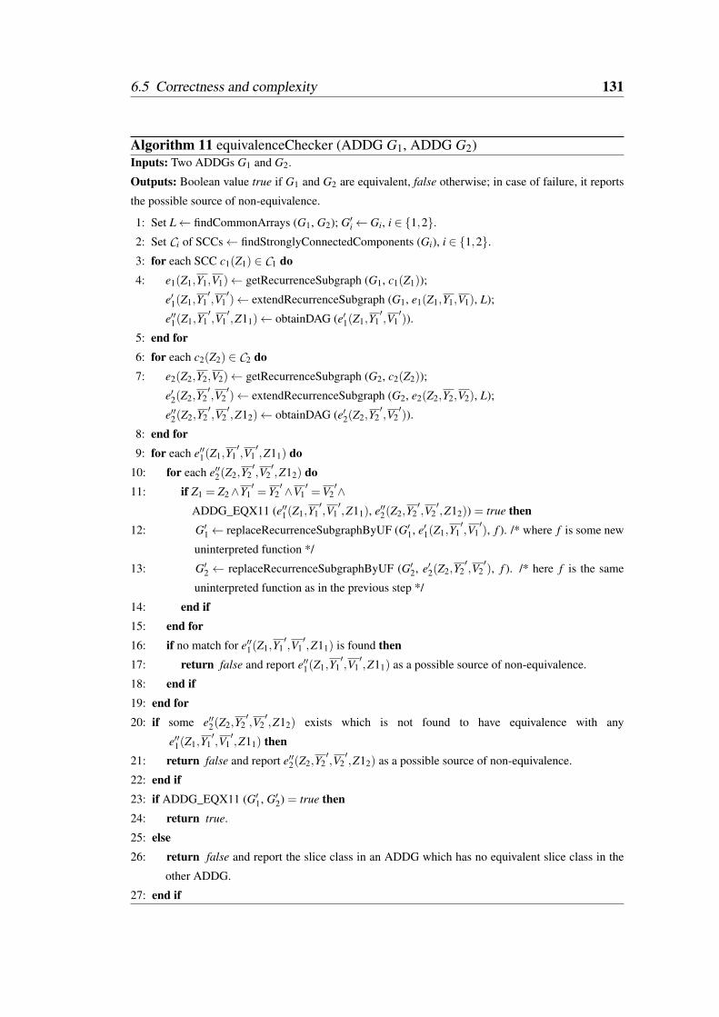
6.5 Correctness and complexity 131
Algorithm 11 equivalenceChecker (ADDG G1, ADDG G2)Inputs: Two ADDGs G1 and G2.
Outputs: Boolean value true if G1 and G2 are equivalent, false otherwise; in case of failure, it reports
the possible source of non-equivalence.
1: Set L← findCommonArrays (G1, G2); G′i← Gi, i ∈ 1,2.2: Set Ci of SCCs← findStronglyConnectedComponents (Gi), i ∈ 1,2.3: for each SCC c1(Z1) ∈ C1 do4: e1(Z1,Y1,V1)← getRecurrenceSubgraph (G1, c1(Z1));
e′1(Z1,Y1′,V1′)← extendRecurrenceSubgraph (G1, e1(Z1,Y1,V1), L);
e′′1(Z1,Y1′,V1′,Z11)← obtainDAG (e′1(Z1,Y1
′,V1′)).
5: end for6: for each c2(Z2) ∈ C2 do7: e2(Z2,Y2,V2)← getRecurrenceSubgraph (G2, c2(Z2));
e′2(Z2,Y2′,V2′)← extendRecurrenceSubgraph (G2, e2(Z2,Y2,V2), L);
e′′2(Z2,Y2′,V2′,Z12)← obtainDAG (e′2(Z2,Y2
′,V2′)).
8: end for9: for each e′′1(Z1,Y1
′,V1′,Z11) do
10: for each e′′2(Z2,Y2′,V2′,Z12) do
11: if Z1 = Z2∧Y1′= Y2
′∧V1′=V2
′∧ADDG_EQX11 (e′′1(Z1,Y1
′,V1′,Z11), e′′2(Z2,Y2
′,V2′,Z12)) = true then
12: G′1← replaceRecurrenceSubgraphByUF (G′1, e′1(Z1,Y1′,V1′), f ). /* where f is some new
uninterpreted function */
13: G′2 ← replaceRecurrenceSubgraphByUF (G′2, e′2(Z2,Y2′,V2′), f ). /* here f is the same
uninterpreted function as in the previous step */
14: end if15: end for16: if no match for e′′1(Z1,Y1
′,V1′,Z11) is found then
17: return false and report e′′1(Z1,Y1′,V1′,Z11) as a possible source of non-equivalence.
18: end if19: end for20: if some e′′2(Z2,Y2
′,V2′,Z12) exists which is not found to have equivalence with any
e′′1(Z1,Y1′,V1′,Z11) then
21: return false and report e′′2(Z2,Y2′,V2′,Z12) as a possible source of non-equivalence.
22: end if23: if ADDG_EQX11 (G′1, G′2) = true then24: return true.
25: else26: return false and report the slice class in an ADDG which has no equivalent slice class in the
other ADDG.
27: end if
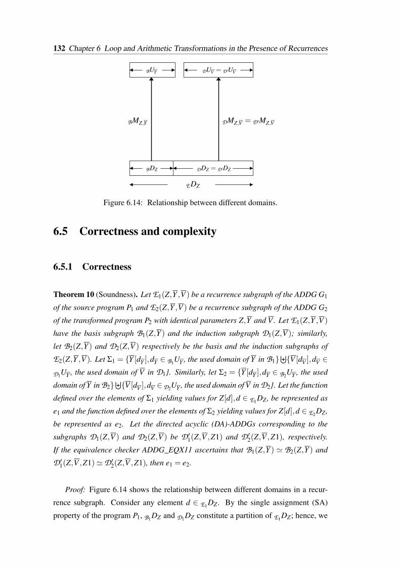
132 Chapter 6 Loop and Arithmetic Transformations in the Presence of Recurrences
DMZ,V = D ′MZ,VBMZ,Y
BDZ
BUY
EDZ
DUV = D ′UV
DDZ = D ′DZ
Figure 6.14: Relationship between different domains.
6.5 Correctness and complexity
6.5.1 Correctness
Theorem 10 (Soundness). Let E1(Z,Y ,V ) be a recurrence subgraph of the ADDG G1
of the source program P1 and E2(Z,Y ,V ) be a recurrence subgraph of the ADDG G2
of the transformed program P2 with identical parameters Z,Y and V . Let E1(Z,Y ,V )
have the basis subgraph B1(Z,Y ) and the induction subgraph D1(Z,V ); similarly,
let B2(Z,Y ) and D2(Z,V ) respectively be the basis and the induction subgraphs of
E2(Z,Y ,V ). Let Σ1 = Y [dY ],dY ∈ B1UY , the used domain of Y in B1⊎V [dV ],dV ∈
D1UY , the used domain of V in D1. Similarly, let Σ2 = Y [dY ],dY ∈ B2UY , the used
domain of Y in B2⊎V [dV ],dV ∈D2UY , the used domain of V in D2. Let the function
defined over the elements of Σ1 yielding values for Z[d],d ∈ E1DZ , be represented as
e1 and the function defined over the elements of Σ2 yielding values for Z[d],d ∈ E2DZ ,
be represented as e2. Let the directed acyclic (DA)-ADDGs corresponding to the
subgraphs D1(Z,V ) and D2(Z,V ) be D ′1(Z,V ,Z1) and D ′2(Z,V ,Z1), respectively.
If the equivalence checker ADDG_EQX11 ascertains that B1(Z,Y ) ' B2(Z,Y ) and
D ′1(Z,V ,Z1)'D ′2(Z,V ,Z1), then e1 = e2.
Proof: Figure 6.14 shows the relationship between different domains in a recur-
rence subgraph. Consider any element d ∈ E1DZ . By the single assignment (SA)
property of the program P1, B1DZ and D1DZ constitute a partition of E1DZ; hence, we
6.5 Correctness and complexity 133
have the following two mutually exclusive cases: (1) d ∈ B1DZ and (2) d ∈ D1DZ . We
carry out proof by cases.
Case 1 [d ∈ B1DZ]: Here,
Z[d] = e1(Y [dY ]), for some dY = B1MZ,Y (d) ∈ B1UY
= rB1(Y [dY ]), where rB1 is the data transformation of the subgraph B1
= rB2(Y [d′Y ]), for some d′Y = B2MZ,Y (d
′) ∈ B2UY
= e2(Y [d′Y ]), since the equivalence checker ADDG_EQX11 ascertains
B1(Z,Y )' B2(Z,Y ), it must have found rB1 = rB2 over the domain
Y [dY ],dY ∈ B1UY = B2UY and
B1MZ,Y = B2MZ,Y over the domains B1DZ = B1DZ
Thus, dY = B1MZ,Y (d) = B2MZ,Y (d′) = d′Y . Hence, from the soundness of DA-ADDG
equivalence checker, e1(Y [dY ]) = e2(Y [dY ]), ∀dY ∈ B1UY = B2UY .
Case 2 [d ∈ D1DZ]: Here,
Z[d] = e1(V [dV ]), where dV = D1MZ,V (d) = D ′1MZ,V (d) ∈ D1UV ,
since by construction of the directed acyclic version D ′1 of D1,
D1MZ,V = D ′1MZ,V over the domain D1DZ = D ′1DZ
= rD ′1(V [dV ],Z1[dZ1]), for some dZ1 ∈ D ′1UZ1 . . .(i)
However, D ′1UZ1(= D1UZ1) ⊆ B1DZ⋃
D ′1DZ (owing to recurrence). Because of SA
property of the program(s), B1DZ⋂
D ′1DZ = /0. Hence we have the following two (mu-
tually exclusive) subcases: (2.1) dZ1 ∈ B1DZ and (2.2) dZ1 ∈ D ′1DZ .
134 Chapter 6 Loop and Arithmetic Transformations in the Presence of Recurrences
Subcase 2.1 [dZ1 ∈ B1DZ]: So, continuing from (i) we have,
Z[d] = e1(V [dV ])
= rD ′1(V [dV ],Z1[dZ1])
= rD ′1(V [dV ],rB1(Y [dY ]))
= rD ′2(V [dV ],rB2(Y [dY ]))
= e2(V [dV ]), for some dV = B1MZ,Y (d) = B2MZ,Y (d)
since the equivalence checker ADDG_EQX11 finds B1MZ,Y (d) = B2MZ,Y (d),
rB1 = rB2 over Y [dY ],dY ∈ B1MZ,Y (B1DZ) = B2MZ,Y (B2DZ) and
rD ′1 = rD ′2 over V [dV ],dV ∈ D1UV = D ′1UV×Z1[dz1],dz1 ∈ D ′1UZ1
Therefore, e1 = e2 for this subcase.
Subcase 2.2 [dZ1 ∈ D ′1DZ]: It may be noted that from Definition 33 (recurrence
array vertex) D1DZ⋂
D1UZ1 = D ′1DZ⋂
D ′1UZ1 6= /0, i.e., some elements of Z defined
through D1 are used in defining further elements of Z in D1 itself. Specifically,
equation (i) Z[d] = e1(V [dV ]) = rD ′1(V [dV ],Z1[dZ1]) depicts that in order to prove
that Z[d] evaluated through e1 is the same as that evaluated through e2, we need to
assume that in D ′1, the evaluation of Z[dZ1] (= Z1[dZ1]) should precede the evalu-
ation of Z[d], and likewise, in D ′2. Such an assumption is nothing but the induc-
tion hypothesis. (This aspect justifies the nomenclature of the subgraphs D1 and D2
as the induction subgraphs because it supports the inductive step in the analysis of
a recurrence.) In other words, an ordering over the elements of D ′1DZ (= D ′2DZ) is
needed for validation of e1 = e2. Towards this, let us consider the following relation:
∀d1,d2 ∈ D ′1DZ (= D ′2DZ), d1 ≺ d2, if the computation of the value of Z[d2] depends
upon the computation of that of Z[d1]2.
Assuming that ∀d′ ≺ d, Z[d′] (= Z1[d′]) are evaluated identically by D ′1 and D ′2,
i.e.,2Such a definition essentially implies that there is a valid schedule, which is supported by the re-
strictions given in Section 6.2.
6.5 Correctness and complexity 135
Z[d′] = e1(V [d′V ]) = e2(V [d′V ]), we have
Z[d] = e1(V [dV ])
= rD ′1(V [dV ],Z1[dZ1])
= rD ′1(V [dV ],e1(V [d′V ])), where d′V = D1MZ,V (d) = D2MZ,V (d)
= rD ′2(V [d′V ],e2(V [d′V ]))
= e2(V [d′V ]), by induction hypothesis and by the equivalence
checker ADDG_EQX11 applied on D ′1 and D ′2
Hence, e1 = e2 over the defined domain D ′1DZ1 =D ′2 DZ1.
6.5.2 Complexity
Let us determine the worst case time complexity of all the steps involved in Algo-
rithm 11. Note that the analysis has been done assuming the number of arrays in each
ADDG is a, the number of statements (write edges) is s, the maximum arity of a func-
tion is t and the number of recurrence subgraphs is γ.
Step 1: Finding the set of common arrays takes a2 time and copying each ADDG takes
O(V +E), i.e., O((a+ s)+(a+ s× t)) time.
Step 2: This step basically involves identification of SCCs in a directed graph using
Tarjan’s algorithm [148], which can be done in a depth-first traversal of the graph.
Therefore, this step also requires O(V +E) = O((a+ s)+(a+ s× t)) time.
Steps 3—5: Each of the three functions mentioned in step 4 requires a depth-first
traversal of the ADDG; therefore, the loop takes O(γ× ((a+ s)+(a+ s× t))) time.
Steps 6—8: Similar to the steps 3—5.
Steps 9—19: In step 11, checking whether the arrays involved in two recurrence sub-
graphs are identical takes O(a2) time. Note that the complexity of comparing two
normalized expressions is O(2‖F‖), where ‖F‖ is the length of a normalized formula
in terms of its constituent variables and operators [88]. However, representing the
data transformation of the elements of the output array of a subgraph in terms of the
elements of the input arrays of that subgraph may require substitution of the interme-
diate temporary arrays in a transitive fashion, which takes O(a2×2‖F‖) time [88]. For
finding the transitive dependence and the union of the mappings, ISL [152] has been
used, whose worst case time complexity is the same as the deterministic upper bound
136 Chapter 6 Loop and Arithmetic Transformations in the Presence of Recurrences
on the time required to verify Presburger formulas, i.e., O(222n), where n = O(t× a)
is the length of the formula; the worst case behaviour, however, is never exhibited
in our experiments. Since we replace the recurrence subgraphs (except for the re-
currence vertex and the input array vertices) with an operator vertex representing an
uninterpreted function along with the edges connecting this operator vertex with the
recurrence vertex and the input array vertices, step 12 takes O(V ) = O(a+ s) time
for each ADDG. We have to compare the data transformations of pairs of recurrence
subgraphs, one from each ADDG; thus, the loop encompassing the steps 9–19 takes
O(g× (2‖F‖+a2×2‖F‖)) time.
Steps 20—22: This step simply reports a failure case; however, in the worst case, the
faulty recurrence subgraph may cover almost the entire ADDG; thus, this step may
also require O(V +E) = O((a+ s)× (a+ s× t)) time.
Steps 23—27: In step 23, the verifier of [88] is invoked; therefore, the time complex-
ity of these steps is O(kn×x× (2‖F‖+ a2× 2‖F‖)+ k2×n×x× 2‖F‖) in the worst case
as reported in [88], where n is the number of branching blocks in the control flow
graph of the program, k is the maximum branches in a branching block and x is the
maximum number of arrays defined in a branch. Since this is the costliest step in the
entire algorithm, the worst case time complexity of Algorithm 11 is identical to the
one reported in [88].
6.6 Experimental results
Our method has been implemented in the C language and run on a 2.0 GHz Intel R©
CoreTM2 Duo machine. The tool is available at http://cse.iitkgp.ac.in/~chitta/pubs/
EquivalenceChecker_ADDG.tar.gz along with the benchmarks, installation and us-
age guidelines. It first constructs the ADDGs from the original and the transformed
behaviours written in C and then applies our method to establish the equivalence be-
tween them. The tool has been tested on some benchmarks. The characteristics of
the benchmarks and the time taken to establish equivalence by our tool and by those
of [154] and [88] are given in Table 6.1; note that the symbol × has been used when-
ever a tool failed to establish the required equivalence. The benchmarks have been ob-
tained by manually applying different transformations to the programs of Sobel edge
detection (SOB), Debaucles 4-coefficient wavelet filter (WAVE), Laplace algorithm
to edge enhancement of northerly directional edges (LAP), linear recurrence solver
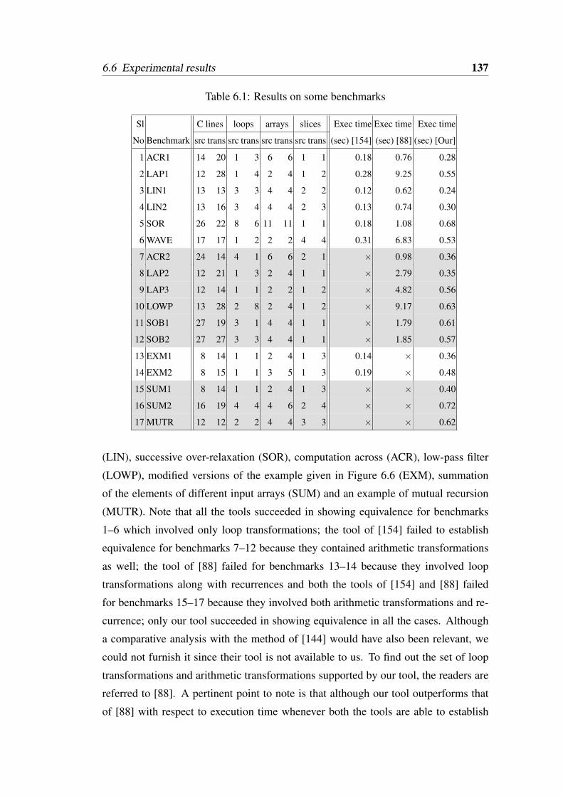
6.6 Experimental results 137
Table 6.1: Results on some benchmarks
Sl C lines loops arrays slices Exec time Exec time Exec time
No Benchmark src trans src trans src trans src trans (sec) [154] (sec) [88] (sec) [Our]
1 ACR1 14 20 1 3 6 6 1 1 0.18 0.76 0.28
2 LAP1 12 28 1 4 2 4 1 2 0.28 9.25 0.55
3 LIN1 13 13 3 3 4 4 2 2 0.12 0.62 0.24
4 LIN2 13 16 3 4 4 4 2 3 0.13 0.74 0.30
5 SOR 26 22 8 6 11 11 1 1 0.18 1.08 0.68
6 WAVE 17 17 1 2 2 2 4 4 0.31 6.83 0.53
7 ACR2 24 14 4 1 6 6 2 1 × 0.98 0.36
8 LAP2 12 21 1 3 2 4 1 1 × 2.79 0.35
9 LAP3 12 14 1 1 2 2 1 2 × 4.82 0.56
10 LOWP 13 28 2 8 2 4 1 2 × 9.17 0.63
11 SOB1 27 19 3 1 4 4 1 1 × 1.79 0.61
12 SOB2 27 27 3 3 4 4 1 1 × 1.85 0.57
13 EXM1 8 14 1 1 2 4 1 3 0.14 × 0.36
14 EXM2 8 15 1 1 3 5 1 3 0.19 × 0.48
15 SUM1 8 14 1 1 2 4 1 3 × × 0.40
16 SUM2 16 19 4 4 4 6 2 4 × × 0.72
17 MUTR 12 12 2 2 4 4 3 3 × × 0.62
(LIN), successive over-relaxation (SOR), computation across (ACR), low-pass filter
(LOWP), modified versions of the example given in Figure 6.6 (EXM), summation
of the elements of different input arrays (SUM) and an example of mutual recursion
(MUTR). Note that all the tools succeeded in showing equivalence for benchmarks
1–6 which involved only loop transformations; the tool of [154] failed to establish
equivalence for benchmarks 7–12 because they contained arithmetic transformations
as well; the tool of [88] failed for benchmarks 13–14 because they involved loop
transformations along with recurrences and both the tools of [154] and [88] failed
for benchmarks 15–17 because they involved both arithmetic transformations and re-
currence; only our tool succeeded in showing equivalence in all the cases. Although
a comparative analysis with the method of [144] would have also been relevant, we
could not furnish it since their tool is not available to us. To find out the set of loop
transformations and arithmetic transformations supported by our tool, the readers are
referred to [88]. A pertinent point to note is that although our tool outperforms that
of [88] with respect to execution time whenever both the tools are able to establish
138 Chapter 6 Loop and Arithmetic Transformations in the Presence of Recurrences
equivalence, the tool of [154] takes about 2.5 times less execution time than that of
ours whenever it is successful – this is probably because our tool invokes ISL [152]
through system call and communicates with it via reading and writing to files whereas,
ISL comes as an integrated package within [154] itself and hence it is faster.
6.7 Conclusion
Loop and arithmetic transformations are applied extensively in embedded system de-
sign to minimize execution time, power, area, etc. An ADDG based equivalence
checking method has been proposed in [86, 88] for translation validation of programs
undergoing such transformations. This method, however, cannot be applied to verify
programs that involve recurrences because recurrences lead to cycles in the ADDGs
which render currently available dependence analyses and arithmetic simplification
rules inadmissible. Another verification technique [153, 154] which can verify pro-
grams with recurrences does not handle arithmetic transformations. The validation
scheme proposed in this chapter isolates the suitable subgraphs (arising from recur-
rences) in the ADDGs from the acyclic portions and treats them separately; each cyclic
subgraph in the original ADDG is compared with its corresponding subgraph in the
transformed ADDG in isolation and if all such pairs of subgraphs are found equiva-
lent, then the entire ADDGs, with the subgraphs replaced by designated uninterpreted
functions of proper arities, are compared in the usual manner of [88]. The soundness
and the complexity of the method have been formally treated. The experimental re-
sults demonstrate the efficacy of the method. Our method, however, cannot resolve
equivalence in the presence of recurrences that employ reductions [75] because re-
ductions involve accumulations of a parametric number of sub-expressions using an
associative and commutative operator. In our future work, we intend to alleviate the
current limitation of the method to handle a more general class of programs.
Chapter 7
Conclusion and Scope for FutureWork
Application of faulty code optimizations may proliferate as software bugs; hence it
is crucial to perform translation validation. To meet this objective, some equivalence
checking techniques have been developed and implemented by us to verify several
code optimizations. In this chapter, we first briefly summarize the contributions of the
work presented in the thesis. Next, we discuss several possible directions/extensions
for future research.
7.1 Summary of contributions
Translation validation of code motion transformations: Code motion transfor-
mations are widely used to improve the performance of programs [48, 65, 66, 82].
Consequently, a lot of investigation has been devoted for verifying such transforma-
tions [95, 100, 104, 110]. Of the different techniques available for verification of code
motion transformations, the path extension based technique [90, 91, 95, 110] which
models programs as FSMDs [58] has been particularly encouraging since it has been
successful in verifying code motion transformations in the presence of non-structure
preserving transformations, i.e., transformations which alter control structures of pro-
grams, such as those introduced by path based schedulers [33, 135]. Moreover, this
technique handles a wide range of arithmetic transformations by employing a normal-
139
140 Chapter 7 Conclusion and Scope for Future Work
ization technique [141] that tries to reduce two computationally equivalent expres-
sions to a syntactically identical form. The path extension based approach, however,
fails in case of verifying code motions across loops because a path, by definition,
cannot be extended beyond a loop [56]. Hence, our initial objective was to develop
an equivalence checking method that alleviates this drawback of the path extension
based approach while retaining all its benefits. We have developed a symbolic value
propagation based equivalence checking method for FSMDs that stores the differ-
ence between the data computations of a pair of paths (obtained from two different
FSMDs whose equivalence we seek to validate) as propagated vectors and propa-
gates these vectors to all the paths originating from the end states of the original path
pair. This process is repeated until all the mismatches encountered have been com-
pensated for during subsequent traversal of the FSMDs; if no mismatch is identified
when the final paths of the two FSMDs have been traversed, then we declare them as
equivalent; otherwise, we rule them as possibly non-equivalent. Note that equivalence
checking of flowchart schemas being an undecidable problem, completeness cannot
be assured. However, the soundness and the termination of our method have been
formally proved. To examine whether our symbolic value propagation based equiva-
lence checking is superior to path extension based equivalence checking, we initially
compared our tool with that of [95] for three different compilers namely, a synthe-
sis tool for structured datapaths [117], a path based scheduler [33] and a high-level
synthesis tool SPARK [64]. For all three compilers, our tool required less time on an
average to establish equivalence than that of [95]. Next, we compared our tool with
that of [90], which is an improvised method of [95], that can additionally handle non-
uniform code motions; our tool was found to take considerably less amount of time
in establishing equivalence for all the benchmarks reported in [90]. Finally, we sub-
jected some benchmarks to SPARK followed by the path based scheduler to perform
optimizations in two successive steps; for those test cases where the target code was
produced from the source code by means of code motions across loops, only our tool
could prove the equivalence. It is important to note that the computational complexity
of the symbolic value propagation based method has been analyzed and found to be no
worse than that for path extension method [90], i.e., our symbolic value propagation
method is capable of handling more sophisticated transformations than [90] without
incurring any extra overhead of time complexity.
Deriving bisimulation relations from path based equivalence checkers: Trans-

7.1 Summary of contributions 141
lation validation by means of deriving bisimulation relations between programs has
been an actively persuaded field of study [103, 104, 126]. Meanwhile, translation
validation through path based equivalence checking has also received similar atten-
tion [22, 90, 95, 110]. Both these techniques have been popular because they pro-
vide benefits which are exclusive to each, while suffering from distinctive draw-
backs. Specifically, bisimulation based methods [103, 104] can handle loop shift-
ing [44], which no path based approach can handle till date, whereas, path based
approaches [22, 90, 95, 110] are adept in handling non-structure preserving transfor-
mations; furthermore, path based approach guarantees termination which bisimulation
based approach cannot. However, the conventionality of bisimulation as the approach
for equivalence checking raises the natural question of examining whether path based
equivalence checking yields a bisimulation relation or not. In this thesis, we have
presented mechanisms to derive bisimulation relations from the outputs of the path
extension based equivalence checker and the symbolic value propagation based equiv-
alence checker whenever two FSMDs are found to be equivalent by these checkers. It
is to be noted that none of the bisimulation relation based approaches has been shown
to tackle code motions across loops; therefore, the present work demonstrates, for the
first time, that a bisimulation relation exists even under such a context.
Translation validation of code motion transformations in array-intensive pro-grams: The FSMD model does not support arrays. As a result, the verifiers built
upon this model are rendered inapplicable while verifying code motion transforma-
tions in array-intensive programs. To alleviate this shortcoming, several ramifications
are needed. First, the FSMD model is extended to the FSMDA model which allows ar-
rays in its datapath. Secondly, the normalization technique of [141] is augmented with
additional grammar rules to represent array references as McCarthy’s functions [120].
Thirdly, the symbolic value propagation based equivalence checker is fitted with the
FSMDA model while accommodating special propagation rules for index variables.
The correctness and the complexity of the verification procedure are formally treated.
To validate that our FSMDA based equivalence checker is capable of verifying code
motion transformations of array-intensive programs, we performed a set of experi-
ments. The benchmark suite comprised behaviours which are computation intensive
and primarily involved arrays. These benchmarks were fed to the SPARK tool [64] to
obtain the transformed behaviours. New scalar variables, but no array variables, are
introduced during the transformations. Our proposed method could ascertain equiva-
142 Chapter 7 Conclusion and Scope for Future Work
lences in all the cases except one; for this case, it reported a possible non-equivalence
and outputted a set of paths (each paired with an almost similar path) for which equiv-
alence could not be found. A scrutiny of the involved benchmark revealed that the
non-equivalence resulted from a bug in the implementation of copy propagation for
array variables in the SPARK tool.
Translation validation of loop and arithmetic transformations in the presence ofrecurrences: Loop and arithmetic transformations are applied extensively in embed-
ded system design to minimize execution time, power, area, etc. [30, 79, 131, 165]. An
equivalence checking method which models programs as ADDGs has been proposed
in [144, 146] for translation validation of programs undergoing loop transformations.
This method is extended later in [86, 88] to verify a plethora of arithmetic transfor-
mations as well. This method, however, cannot be applied to verify programs that
involve recurrences because recurrences lead to cycles in the ADDGs which render
currently available dependence analyses and arithmetic simplification rules inadmis-
sible. Another verification technique [154] which can verify programs with recur-
rences does not handle arithmetic transformations. Therefore, we aimed at developing
a unified equivalence checking framework to cover the entire spectrum of loop and
arithmetic transformations in addition to recurrences by further extending the ADDG
based equivalence checking strategy. Our method initially segregates the subgraphs
representing recurrences in an ADDG from the cycle-free subgraphs and basically
tries to find pairs of such recurrence subgraphs, one from the original ADDG and the
other from the transformed ADDG, which have undergone equivalent functional trans-
formation; on finding a match, it substitutes the recurrence subgraphs in either ADDG
with an identical uninterpreted function; once all recurrence subgraphs in an ADDG
have been successfully paired up with recurrence subgraphs from the other ADDG and
subsequently substituted by uninterpreted functions, the equivalence checker of [88] is
applied on the modified ADDGs (which no longer contain cycles) to test their equiva-
lence. The correctness of the proposed method is formally proved and the complexity
is analyzed. The experimental results attest the effectiveness of the method; while
the method of [154] is able to establish equivalence in cases where the transformed
behaviour is obtained from the original by application of loop transformations and
recurrences (but no arithmetic transformation), the method of [88] can prove equiv-
alence in cases of loop and arithmetic transformations (but no recurrence); only our
method can establish equivalence is presence of loop and arithmetic transformations
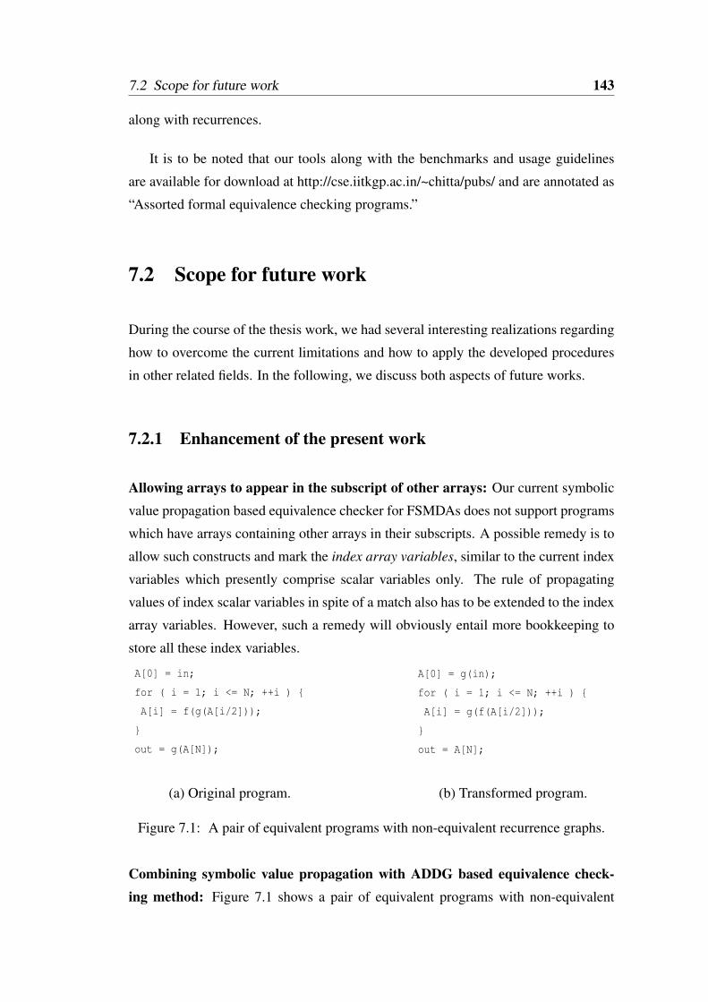
7.2 Scope for future work 143
along with recurrences.
It is to be noted that our tools along with the benchmarks and usage guidelines
are available for download at http://cse.iitkgp.ac.in/~chitta/pubs/ and are annotated as
“Assorted formal equivalence checking programs.”
7.2 Scope for future work
During the course of the thesis work, we had several interesting realizations regarding
how to overcome the current limitations and how to apply the developed procedures
in other related fields. In the following, we discuss both aspects of future works.
7.2.1 Enhancement of the present work
Allowing arrays to appear in the subscript of other arrays: Our current symbolic
value propagation based equivalence checker for FSMDAs does not support programs
which have arrays containing other arrays in their subscripts. A possible remedy is to
allow such constructs and mark the index array variables, similar to the current index
variables which presently comprise scalar variables only. The rule of propagating
values of index scalar variables in spite of a match also has to be extended to the index
array variables. However, such a remedy will obviously entail more bookkeeping to
store all these index variables.
A[0] = in;
for ( i = 1; i <= N; ++i )
A[i] = f(g(A[i/2]));
out = g(A[N]);
(a) Original program.
A[0] = g(in);
for ( i = 1; i <= N; ++i )
A[i] = g(f(A[i/2]));
out = A[N];
(b) Transformed program.
Figure 7.1: A pair of equivalent programs with non-equivalent recurrence graphs.
Combining symbolic value propagation with ADDG based equivalence check-ing method: Figure 7.1 shows a pair of equivalent programs with non-equivalent
144 Chapter 7 Conclusion and Scope for Future Work
recurrence subgraphs. Since the basis subgraphs and the induction subgraphs of the
programs are different, our ADDG based equivalence checker will declare them to
be possibly non-equivalent. However, an equivalence checking mechanism may be
devised that propagates the mismatched symbolic values in and g(in) from the basis
subgraphs to the induction subgraphs and even out of the recurrence subgraph, if re-
quired (as in the present scenario). Note that the method of [154] is able to establish
equivalence of the two programs given in Figure 7.1 by employing a similar technique.
Attending currently unaddressed programming constructs: Here we present some
of the ways in which our present equivalence checking frameworks can be extended
to encompass currently unaddressed programming constructs.
Unsupported datatypes: The normalization technique employed by our path based
equivalence checkers reduces many computationally equivalent expressions to a syn-
tactically identical form. In order to compare the path characteristics, their condi-
tions of execution and data transformations are represented in this normalized form.
However, the present normalization grammar has no rules to represent bit-vectors and
user-defined datatypes. An SMT solver can be used to overcome these drawbacks.
This problem has been explored by us in [23] where we experimented with three SMT
solvers – Yices2, CVC4 and Z3. A pertinent point to note is that whenever the nor-
malization technique was able to establish equivalence its execution time was found
to be less than those involving SMT solvers. This observation indicates that reducing
two expressions to identical structural form (using normalization) to determine their
equivalence is a less time-consuming process than applying algebraic simplification
rules (such as those employed by the SMT solvers reported in this work) for the same.
So, we think it is better to invoke an SMT solver only when the normalizer is found to
be inadequate in establishing equivalence between two expressions, i.e., use an SMT
solver to supplement the normalizer and not to replace it. A full fledged implementa-
tion of such an amalgamated equivalence checker still remains as a future work.
Pointers and dynamic memory allocation: We envision that posterior to alias analy-
sis if pointers are replaced by the actual storage variables that they point to, such as,
∗(p+ i) is converted to p[i] where p is the base address of an array and i represents an
index, then our equivalence checking procedures can be applied as usual. For dynamic
memory allocation, fragmentation and garbage collection presents further complica-
cies. The Memcheck tool in the Valgrind tool suite [8] addresses many of the invalid
memory access issues. Once the validity of the memory accesses are ascertained then
7.2 Scope for future work 145
our tools may be used.
Inter-procedural analysis: The equivalence checking procedures described in this the-
sis compare one function from the original program with one from the transformed
program. In the scenario where we want to check equivalence between an original
and a transformed program comprising multiple functions, we may do so by checking
equivalence between pairs of programs (one from the original program and the other
from the transformed program) in a bottom-up fashion, i.e., we start with the func-
tions which which have no dependency on any of the other functions before moving
on to those which have dependencies on the functions which are already proved to
be equivalent. Note that the functions can be paired easily based on their names be-
cause typically compilers do not rename functions. In case our equivalence checker is
employed to verify semi-automated or hand-optimized programs where some of the
functions may have been split or merged in the transformed version, one may inline
the functions within one main function and then apply our equivalence checker from
program verification. Of course, inlining may not be viable always, especially in the
presence of recursive functions, and in such a case our method may not be applicable.
Concurrency: In a scenario where thread-safety guarantees that the code is free of race
conditions, i.e., the final values stored can be accurately computed, our equivalence
checking technique may be applied to check equivalence between the original sequen-
tial code and the transformed parallel code where only one schedule of the threads
is considered. Otherwise, path based equivalence checking methods using Petri net
based models, which can effectively capture concurrency, may be used [18, 19].
7.2.2 Scope of application to other research areas
Evolving programs: Although the present thesis deals with validation of code op-
timizations that are commonly applied by compilers, the scope of checking equiva-
lence between programs may include other domains as well where the transformed
programs have been obtained by some other means. One such domain is evolving
programs; software is not written entirely from scratch, it rather evolves over time.
Often industrial software development projects release different versions of the same
software; validation of such evolving programs to ensure compatibility between these
versions remains a huge problem [133]. An interesting study would be to check the
applicability of the formal methods developed in this thesis to establish equivalence
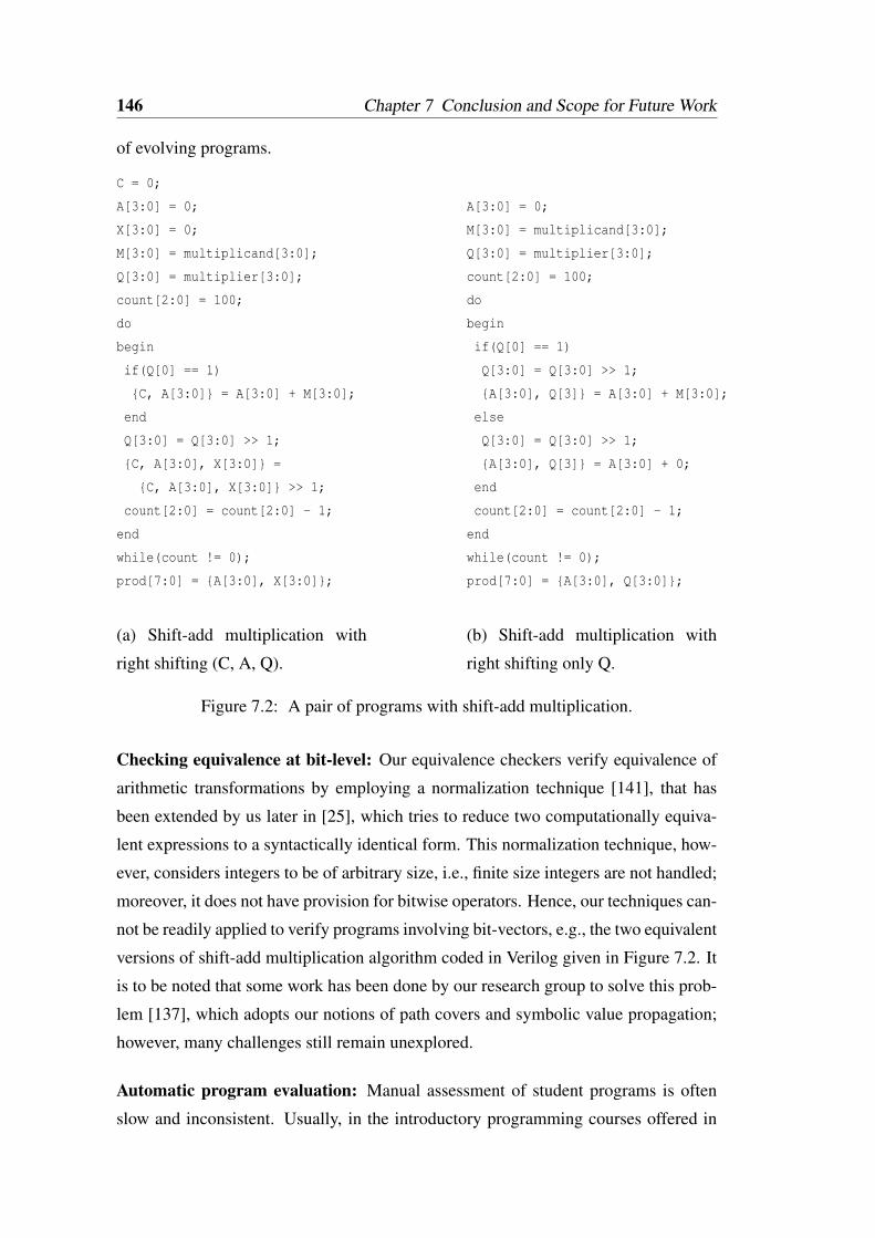
146 Chapter 7 Conclusion and Scope for Future Work
of evolving programs.
C = 0;
A[3:0] = 0;
X[3:0] = 0;
M[3:0] = multiplicand[3:0];
Q[3:0] = multiplier[3:0];
count[2:0] = 100;
do
begin
if(Q[0] == 1)
C, A[3:0] = A[3:0] + M[3:0];
end
Q[3:0] = Q[3:0] >> 1;
C, A[3:0], X[3:0] =
C, A[3:0], X[3:0] >> 1;
count[2:0] = count[2:0] - 1;
end
while(count != 0);
prod[7:0] = A[3:0], X[3:0];
(a) Shift-add multiplication with
right shifting (C, A, Q).
A[3:0] = 0;
M[3:0] = multiplicand[3:0];
Q[3:0] = multiplier[3:0];
count[2:0] = 100;
do
begin
if(Q[0] == 1)
Q[3:0] = Q[3:0] >> 1;
A[3:0], Q[3] = A[3:0] + M[3:0];
else
Q[3:0] = Q[3:0] >> 1;
A[3:0], Q[3] = A[3:0] + 0;
end
count[2:0] = count[2:0] - 1;
end
while(count != 0);
prod[7:0] = A[3:0], Q[3:0];
(b) Shift-add multiplication with
right shifting only Q.
Figure 7.2: A pair of programs with shift-add multiplication.
Checking equivalence at bit-level: Our equivalence checkers verify equivalence of
arithmetic transformations by employing a normalization technique [141], that has
been extended by us later in [25], which tries to reduce two computationally equiva-
lent expressions to a syntactically identical form. This normalization technique, how-
ever, considers integers to be of arbitrary size, i.e., finite size integers are not handled;
moreover, it does not have provision for bitwise operators. Hence, our techniques can-
not be readily applied to verify programs involving bit-vectors, e.g., the two equivalent
versions of shift-add multiplication algorithm coded in Verilog given in Figure 7.2. It
is to be noted that some work has been done by our research group to solve this prob-
lem [137], which adopts our notions of path covers and symbolic value propagation;
however, many challenges still remain unexplored.
Automatic program evaluation: Manual assessment of student programs is often
slow and inconsistent. Usually, in the introductory programming courses offered in
7.2 Scope for future work 147
institutions with a large intake of students, a lot of assessment work has to be done
manually by the instructors. As an example, at IIT Kharagpur where introductory
programming course is offered to around 600 students in every semester, each student
has to submit around 10–12 assignments and each assessment has about 10 program-
ming exercises. Thus, the evaluation task becomes as enormous as checking around
1,20,000 programs in a year. Assessment speed can be improved along with consis-
tency by automating the process of evaluation. Hence, it is desirable to develop tools
for automated evaluation of programming assignments. A survey on automated as-
sessment of programs can be found in [11]. An automated program evaluation scheme
by leveraging the equivalence checking method of FSMDs is presented in [143], where
a student program is compared with the program supplied by the instructor, both mod-
eled as FSMDs. However, a lot more headway is still required for this problem to
reach a full-fledged deployment.

Appendix A
Construction of FSMDAs fromBehavioural Descriptions
This appendix gives a brief elucidation for obtaining FSMDAs from behavioural de-
scriptions (high-level languages), such as C, and how to represent them textually so
that they can be fed as inputs to our FSMDA equivalence checker. Note that the con-
tent of section A.1 of this manuscript is largely borrowed from [90].
A.1 How to represent behavioural descriptions as FS-
MDAs conceptually
Any (sequential) behaviour consists of a combination of the following three basic con-
structs: (i) sequences of statements without any bifurcation of control flow, i.e., Basic
Blocks (BBs), (ii) if-else constructs, i.e., Control Blocks (CBs), and (iii) loops. There-
fore, without any loss of generality, capturing these three constructs in an FSMDA
model enables us to effectively represent any sequential behaviour as an FSMDA.
A BB consisting of a sequence of n statements S1, . . . ,Sn, can be represented as a
sequence of n+1 states q0, . . . ,qn, say and n edges of the form q j−1−/S j−−−−− q j,1 ≤
j ≤ n, in the corresponding FSMDA. The number of states in the FSMDA, however,
can be reduced in the following way (although it is not mandatory).
149
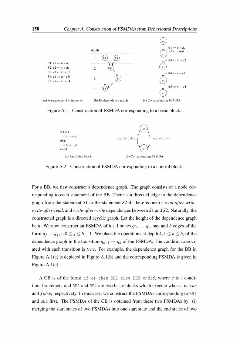
150 Chapter A Construction of FSMDAs from Behavioural Descriptions
S1: t1⇐ u×d;S2: t2⇐ x+d;S3: t3⇐ t1× t2;S4: t4⇐ u− t3;S5: t5⇐ t1× t4;
depth
1
2
3
4
S1 S2
S3
S4
S5
(b) Its dependence graph. (c) Corresponding FSMDA.(a) A sequence of statements.
q0
q1
q2
q3
q4
−/t3⇐ t1× t2
−/t1⇐ u×d,
−/t4⇐ u− t3
−/t5⇐ t1× t4
t2⇐ x+d
Figure A.1: Construction of FSMDA corresponding to a basic block.
a⇐ x+ y;else
a⇐ x− y;
if ( c )
¬c/a⇐ x− y
q0
q1
(b) Corresponding FSMDA.(a) An if-else block.
endif
c/a⇐ x+ y
Figure A.2: Construction of FSMDA corresponding to a control block.
For a BB, we first construct a dependence graph. The graph consists of a node cor-
responding to each statement of the BB. There is a directed edge in the dependence
graph from the statement S1 to the statement S2 iff there is one of read-after-write,
write-after-read, and write-after-write dependences between S1 and S2. Naturally, the
constructed graph is a directed acyclic graph. Let the height of the dependence graph
be h. We now construct an FSMDA of h+1 states q0, . . . ,qh, say and h edges of the
form q j q j+1,0 ≤ j ≤ h−1. We place the operations at depth k,1 ≤ k ≤ h, of the
dependence graph in the transition qk−1 qk of the FSMDA. The condition associ-
ated with each transition is true. For example, the dependence graph for the BB in
Figure A.1(a) is depicted in Figure A.1(b) and the corresponding FSMDA is given in
Figure A.1(c).
A CB is of the form: if(c) then BB1 else BB2 endif, where c is a condi-
tional statement and BB1 and BB2 are two basic blocks which execute when c is true
and f alse, respectively. In this case, we construct the FSMDAs corresponding to BB1
and BB2 first. The FSMDA of the CB is obtained from these two FSMDAs by: (i)
merging the start states of two FSMDAs into one start state and the end states of two
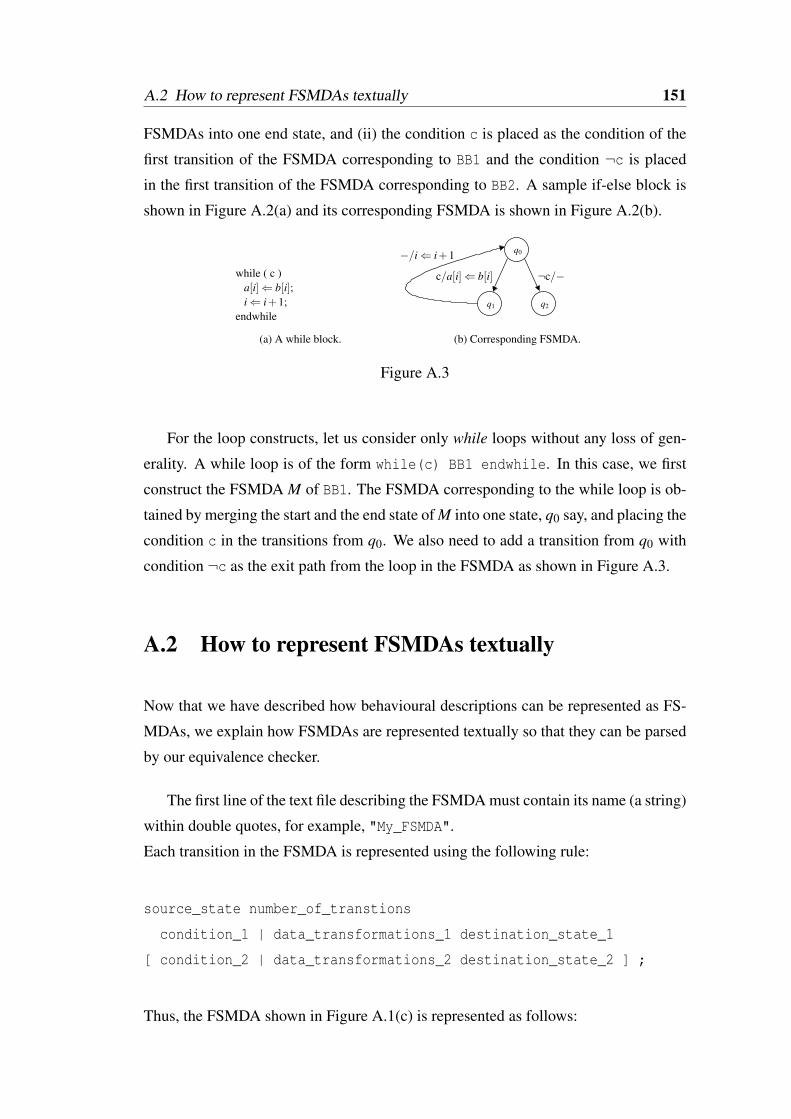
A.2 How to represent FSMDAs textually 151
FSMDAs into one end state, and (ii) the condition c is placed as the condition of the
first transition of the FSMDA corresponding to BB1 and the condition ¬c is placed
in the first transition of the FSMDA corresponding to BB2. A sample if-else block is
shown in Figure A.2(a) and its corresponding FSMDA is shown in Figure A.2(b).
while ( c )a[i]⇐ b[i];i⇐ i+1;
endwhile
(a) A while block.
q0
q1 q2
(b) Corresponding FSMDA.
−/i⇐ i+1
c/a[i]⇐ b[i] ¬c/−
Figure A.3
For the loop constructs, let us consider only while loops without any loss of gen-
erality. A while loop is of the form while(c) BB1 endwhile. In this case, we first
construct the FSMDA M of BB1. The FSMDA corresponding to the while loop is ob-
tained by merging the start and the end state of M into one state, q0 say, and placing the
condition c in the transitions from q0. We also need to add a transition from q0 with
condition ¬c as the exit path from the loop in the FSMDA as shown in Figure A.3.
A.2 How to represent FSMDAs textually
Now that we have described how behavioural descriptions can be represented as FS-
MDAs, we explain how FSMDAs are represented textually so that they can be parsed
by our equivalence checker.
The first line of the text file describing the FSMDA must contain its name (a string)
within double quotes, for example, "My_FSMDA".
Each transition in the FSMDA is represented using the following rule:
source_state number_of_transtions
condition_1 | data_transformations_1 destination_state_1
[ condition_2 | data_transformations_2 destination_state_2 ] ;
Thus, the FSMDA shown in Figure A.1(c) is represented as follows:
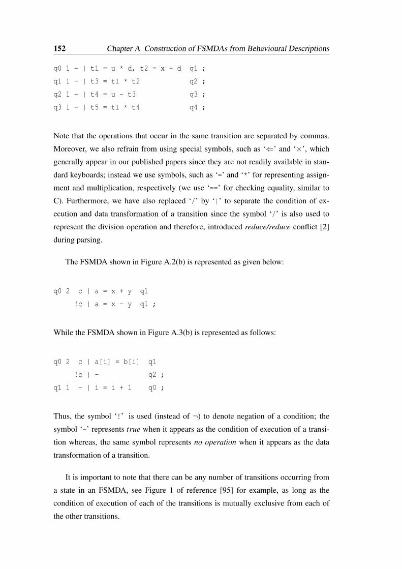
152 Chapter A Construction of FSMDAs from Behavioural Descriptions
q0 1 - | t1 = u * d, t2 = x + d q1 ;
q1 1 - | t3 = t1 * t2 q2 ;
q2 1 - | t4 = u - t3 q3 ;
q3 1 - | t5 = t1 * t4 q4 ;
Note that the operations that occur in the same transition are separated by commas.
Moreover, we also refrain from using special symbols, such as ‘⇐’ and ‘×’, which
generally appear in our published papers since they are not readily available in stan-
dard keyboards; instead we use symbols, such as ‘=’ and ‘*’ for representing assign-
ment and multiplication, respectively (we use ‘==’ for checking equality, similar to
C). Furthermore, we have also replaced ‘/’ by ‘|’ to separate the condition of ex-
ecution and data transformation of a transition since the symbol ‘/’ is also used to
represent the division operation and therefore, introduced reduce/reduce conflict [2]
during parsing.
The FSMDA shown in Figure A.2(b) is represented as given below:
q0 2 c | a = x + y q1
!c | a = x - y q1 ;
While the FSMDA shown in Figure A.3(b) is represented as follows:
q0 2 c | a[i] = b[i] q1
!c | - q2 ;
q1 1 - | i = i + 1 q0 ;
Thus, the symbol ‘!’ is used (instead of ¬) to denote negation of a condition; the
symbol ‘-’ represents true when it appears as the condition of execution of a transi-
tion whereas, the same symbol represents no operation when it appears as the data
transformation of a transition.
It is important to note that there can be any number of transitions occurring from
a state in an FSMDA, see Figure 1 of reference [95] for example, as long as the
condition of execution of each of the transitions is mutually exclusive from each of
the other transitions.
A.2 How to represent FSMDAs textually 153
The following operation depicts that the value read from port P is stored in the variable
v:
read( v, P )
Similarly, the following operation depicts that the expression e is written into port P:
write( P, e )
The users are requested not to confuse these read and write operations with those
of McCarthy’s read/write operations [120] that are associated with arrays; the inter-
nal representation of array expressions using McCarthy’s read/write operations by our
equivalence checker is handled in a different manner than the read and write oper-
ations involving ports. Lastly, a final state (having a single transition, with true as its
condition of execution and no operation as its data transformation, back to the reset
state), qL say, in an FSMDA is represented as follows:
qL 0 ;

Bibliography
[1] ACL2 Version 6.1. http://www.cs.utexas.edu/~moore/acl2/.
[2] Bison: Reduce/Reduce Conflicts. https://www.gnu.org/software/bison/manual/
html_node/Reduce_002fReduce.html.
[3] CVC4 - the smt solver. http://cvc4.cs.nyu.edu/web/.
[4] GCC, the GNU Compiler Collection. https://gcc.gnu.org/.
[5] The llvm compiler infrastructure. http://llvm.org/.
[6] PVS Specification and Verification System. http://pvs.csl.sri.com/.
[7] The Yices SMT Solver. http://yices.csl.sri.com/.
[8] Valgrind. http://valgrind.org/.
[9] Z3. http://z3.codeplex.com/.
[10] A. V. Aho, M. S. Lam, R. Sethi, and J. D. Ullman. Compilers: Princiles,
Techniques, and Tools. Pearson Education, 2006.
[11] K. M. Ala-Mutka. A survey of automated assessment approaches for program-
ming assignments. Computer Science Education, 15(2):83–102, 2005.
[12] R. Allen and K. Kennedy. Optimizing Compilers for Modern Architectures.
Morgan Kaufmann Publishers, 2001.
[13] D. F. Bacon, S. L. Graham, and O. J. Sharp. Compiler transformations for
high-performance computing. ACM Comput. Surv., 26:345–420, 1994.
155
156 BIBLIOGRAPHY
[14] C. Baier. Polynomial time algorithms for testing probabilistic bisimulation and
simulation. In Computer Aided Verification, pages 50–61, 1996.
[15] C. Baier, B. Engelen, and M. E. Majster-Cederbaum. Deciding bisimilarity
and similarity for probabilistic processes. J. Comput. Syst. Sci., 60(1):187–231,
2000.
[16] C. Baier and J.-P. Katoen. Principles of model checking. MIT Press, 2008.
[17] S. Bandyopadhyay, K. Banerjee, D. Sarkar, and C. Mandal. Translation val-
idation for PRES+ models of parallel behaviours via an FSMD equivalence
checker. In Progress in VLSI Design and Test, pages 69–78, 2012.
[18] S. Bandyopadhyay, D. Sarkar, K. Banerjee, and C. Mandal. A path-based equiv-
alence checking method for petri net based models of programs. In Interna-
tional Conference on Software Engineering and Applications,, pages 319–329,
2015.
[19] S. Bandyopadhyay, D. Sarkar, and C. Mandal. An efficient equivalence check-
ing method for petri net based models of programs. In International Conference
on Software Engineering, pages 827–828, 2015.
[20] K. Banerjee. An equivalence checking mechanism for handling recurrences in
array-intensive programs. In Principles of Programming Languages: Student
Research Competition, pages 1–2, 2015.
[21] K. Banerjee, C. Karfa, D. Sarkar, and C. Mandal. A value propagation based
equivalence checking method for verification of code motion techniques. In
International Symposium on Electronic System Design, pages 67–71, 2012.
[22] K. Banerjee, C. Karfa, D. Sarkar, and C. Mandal. Verification of code motion
techniques using value propagation. IEEE Trans. on CAD of ICS, 33(8):1180–
1193, 2014.
[23] K. Banerjee, C. Mandal, and D. Sarkar. Extending the scope of translation
validation by augmenting path based equivalence checkers with smt solvers. In
VLSI Design and Test, 18th International Symposium on, pages 1–6, July 2014.
[24] K. Banerjee, C. Mandal, and D. Sarkar. Deriving bisimulation relations from
path extension based equivalence checkers. In WEPL, pages 1–2, 2015.
BIBLIOGRAPHY 157
[25] K. Banerjee, D. Sarkar, and C. Mandal. Extending the FSMD framework for
validating code motions of array-handling programs. IEEE Trans. on CAD of
ICS, 33(12):2015–2019, 2014.
[26] G. Barany and A. Krall. Optimal and heuristic global code motion for minimal
spilling. In Compiler Construction, pages 21–40, 2013.
[27] C. W. Barrett, Y. Fang, B. Goldberg, Y. Hu, A. Pnueli, and L. D. Zuck. Tvoc: A
translation validator for optimizing compilers. In Computer Aided Verification,
pages 291–295, 2005.
[28] D. Barthou, P. Feautrier, and X. Redon. On the equivalence of two systems of
affine recurrence equations (research note). In Euro-Par Conference on Parallel
Processing, pages 309–313, 2002.
[29] S. Blazy and X. Leroy. Mechanized semantics for the Clight subset of the C
language. J. Autom. Reasoning, 43(3):263–288, 2009.
[30] Y. Bouchebaba, B. Girodias, G. Nicolescu, E. M. Aboulhamid, B. Lavigueur,
and P. G. Paulin. MPSoC memory optimization using program transformation.
ACM Trans. Design Autom. Electr. Syst., 12(4):43:1–43:39, 2007.
[31] F. Brandner and Q. Colombet. Elimination of parallel copies using code mo-
tion on data dependence graphs. Computer Languages, Systems & Structures,
39(1):25–47, 2013.
[32] C. Brandolese, W. Fornaciari, F. Salice, and D. Sciuto. Analysis and modeling
of energy reducing source code transformations. In Design, Automation and
Test in Europe, pages 306–311, 2004.
[33] R. Camposano. Path-based scheduling for synthesis. IEEE Trans. on CAD of
ICS, 10(1):85–93, 1991.
[34] F. Catthoor, E. D., and S. S. Greff. HICSS. Custom Memory Management
Methodology: Exploration of Memory Organisation for Embedded Multime-
dia System Design. Kluwer Academic Publishers, 1998.
[35] G. Chen, M. Kandemir, and F. Li. Energy-aware computation duplication for
improving reliability in embedded chip multiprocessors. In Asia and South
Pacific Design Automation Conference, pages 134–139, 2006.
158 BIBLIOGRAPHY
[36] T.-H. Chiang and L.-R. Dung. Verification method of dataflow algorithms in
high-level synthesis. J. Syst. Softw., 80(8):1256–1270, 2007.
[37] A. Chutinan and B. H. Krogh. Verification of infinite-state dynamic systems
using approximate quotient transition systems. IEEE Trans. Automat. Contr.,
46(9):1401–1410, 2001.
[38] A. Cimatti, E. Clarke, F. Giunchiglia, and M. Roveri. Nusmv: a new sym-
bolic model checker. International Journal on Software Tools for Technology
Transfer, 2:410–425, 2000.
[39] J. Cong, P. Zhang, and Y. Zou. Combined loop transformation and hierarchy al-
location for data reuse optimization. In International Conference on Computer-
Aided Design, pages 185–192, 2011.
[40] J. Cong, P. Zhang, and Y. Zou. Optimizing memory hierarchy allocation with
loop transformations for high-level synthesis. In Design Automation Confer-
ence, pages 1233–1238, 2012.
[41] R. Cordone, F. Ferrandi, M. D. Santambrogio, G. Palermo, and D. Sciuto. Us-
ing speculative computation and parallelizing techniques to improve scheduling
of control based designs. In Asia and South Pacific Design Automation Confer-
ence, pages 898–904, 2006.
[42] T. H. Cormen, C. E. Leiserson, R. L. Rivest, and C. Stein. Introduction to
Algorithms, Second Edition. The MIT Press and McGraw-Hill Book Company,
2001.
[43] L. A. Cortés, P. Eles, and Z. Peng. Verification of embedded systems using a
petri net based representation. In Proceedings of the 13th International Sympo-
sium on System Synthesis, pages 149–156, 2000.
[44] A. Darte and G. Huard. Loop shifting for loop compaction. J. Parallel Pro-
gramming, 28(5):499–534, 2000.
[45] R. De Nicola, A. Fantechi, S. Gnesi, and G. Ristori. An action based frame-
work for verifying logical and behavioural properties of concurrent systems. In
Computer Aided Verification, pages 37–47, 1991.
BIBLIOGRAPHY 159
[46] P. C. Diniz and J. M. P. Cardoso. Code transformations for embedded recon-
figurable computing architectures. In Generative and Transformational Tech-
niques in Software Engineering III, pages 322–344, 2009.
[47] L. C. V. Dos Santos, M. J. M. Heijligers, C. A. J. Van Eijk, J. Van Eijnhoven,
and J. A. G. Jess. A code-motion pruning technique for global scheduling. ACM
Trans. Des. Autom. Electron. Syst., 5(1):1–38, 2000.
[48] L. C. V. Dos. Santos and J. Jress. A reordering technique for efficient code
motion. In Design Automation Conference, pages 296–299, 1999.
[49] A. Dovier, C. Piazza, and A. Policriti. An efficient algorithm for computing
bisimulation equivalence. Theor. Comput. Sci., 311(1-3):221–256, 2004.
[50] A. P. N. E. Özer and D. Gregg. Classification of compiler optimizations for
high performance, small area and low power in fpgas. Technical report, Trinity
College, Dublin, Ireland, Department of Computer Science, 2003.
[51] H. Eveking, H. Hinrichsen, and G. Ritter. Automatic verification of scheduling
results in high-level synthesis. In Design, Automation and Test in Europe, pages
260–265, 1999.
[52] H. Falk and P. Marwedel. Source code optimization techniques for data flow
dominated embedded software. Kluwer, 2004.
[53] J. Fernandez and L. Mounier. "on the fly" verification of behavioural equiva-
lences and preorders. In Computer Aided Verification, pages 181–191, 1991.
[54] J. Fisher. Trace scheduling: A technique for global microcode compaction.
IEEE Transactions on Computers, C-30(7):478–490, 1981.
[55] K. Fisler and M. Y. Vardi. Bisimulation minimization in an automata-theoretic
verification framework. In Formal Methods in Computer-Aided Design, pages
115–132, 1998.
[56] R. W. Floyd. Assigning meaning to programs. In Proceedings the 19th Sympo-
sium on Applied Mathematics, pages 19–32, 1967.
[57] A. Fraboulet, K. Kodary, and A. Mignotte. Loop fusion for memory space
optimization. In International Symposium on Systems Synthesis, pages 95–100,
2001.
160 BIBLIOGRAPHY
[58] D. D. Gajski, N. D. Dutt, A. C. Wu, and S. Y. Lin. High-Level Synthesis:
Introduction to Chip and System Design. Kluwer Academic, 1992.
[59] M. Ghodrat, T. Givargis, and A. Nicolau. Control flow optimization in loops
using interval analysis. In Proceedings of the 2008 international conference on
Compilers, architectures and synthesis for embedded systems, pages 157–166,
2008.
[60] M. Ghodrat, T. Givargis, and A. Nicolau. Optimizing control flow in loops
using interval and dependence analysis. Design Automation for Embedded Sys-
tems, 13:193–221, 2009.
[61] R. Gupta and M. Soffa. Region scheduling: an approach for detecting and redis-
tributing parallelism. IEEE Transactions on Software Engineering, 16(4):421–
431, 1990.
[62] S. Gupta, N. Dutt, R. Gupta, and A. Nicolau. Dynamic conditional branch bal-
ancing during the high-level synthesis of control-intensive designs. In Design,
Automation and Test in Europe, pages 270–275, 2003.
[63] S. Gupta, N. Dutt, R. Gupta, and A. Nicolau. Dynamically increasing the scope
of code motions during the high-level synthesis of digital circuits. IEE Pro-
ceedings: Computer and Digital Technique, 150(5):330–337, 2003.
[64] S. Gupta, N. Dutt, R. Gupta, and A. Nicolau. SPARK: A high-level synthesis
framework for applying parallelizing compiler transformations. In VLSI De-
sign, pages 461–466, 2003.
[65] S. Gupta, N. Dutt, R. Gupta, and A. Nicolau. Using global code motions to
improve the quality of results for high-level synthesis. IEEE Trans. on CAD of
ICS, 23(2):302–312, Feb 2004.
[66] S. Gupta, R. Gupta, N. Dutt, and A. Nicolau. Coordinated parallelizing com-
piler optimizations and high-level synthesis. ACM Trans on Design Automation
of Electronic Systems, 9(4):1–31, 2004.
[67] S. Gupta, R. K. Gupta, M. Miranda, and F. Catthoor. Analysis of high-level
address code transformations for programmable processors. In Design, Au-
tomation and Test in Europe, pages 9–13, 2000.
BIBLIOGRAPHY 161
[68] S. Gupta, M. Reshadi, N. Savoiu, N. Dutt, R. Gupta, and A. Nicolau. Dynamic
common sub-expression elimination during scheduling in high-level synthesis.
In Proceedings of the 15th International Symposium on System Synthesis, pages
261–266, 2002.
[69] S. Gupta, N. Savoiu, N. Dutt, R. Gupta, and A. Nicolau. Conditional spec-
ulation and its effects on performance and area for high-level synthesis. In
International Symposium on System Synthesis, pages 171–176, 2001.
[70] S. Gupta, N. Savoiu, S. Kim, N. Dutt, R. Gupta, and A. Nicolau. Specula-
tion techniques for high level synthesis of control intensive designs. In Design
Automation Conference, pages 269–272, 2001.
[71] R. A. Hernandez, M. Strum, and W. J. Chau. Transformations on the FSMD of
the RTL code with combinational logic statements for equivalence checking of
HLS. In Latin-American Test Symposium, pages 1–6, 2015.
[72] Y. Hu, C. W. Barrett, B. Goldberg, and A. Pnueli. Validating more loop opti-
mizations. Electr. Notes Theor. Comput. Sci., 141(2):69–84, 2005.
[73] C. Hur, D. Dreyer, G. Neis, and V. Vafeiadis. The marriage of bisimulations
and kripke logical relations. In Principles of Programming Languages, pages
59–72, 2012.
[74] W. M. W. Hwu, S. A. Mahlke, W. Y. Chen, P. P. Chang, N. J. Warter, R. A.
Bringmann, R. G. Ouellette, R. E. Hank, T. Kiyohara, G. E. Haab, J. G. Holm,
and D. M. Lavery. The superblock: An effective technique for vliw and super-
scalar compilation. The Journal of Supercomputing, 7:229–248, 1993.
[75] G. Iooss, C. Alias, and S. V. Rajopadhye. On program equivalence with reduc-
tions. In Static Analysis, pages 168–183, 2014.
[76] R. Jain, A. Majumdar, A. Sharma, and H. Wang. Empirical evaluation of some
high-level synthesis scheduling heuristics. In Design Automation Conference,
pages 686–689, 1991.
[77] N. E. Johnson. Code Size Optimization for Embedded Processors. PhD thesis,
University of Cambridge, 2004.
[78] I. Kadayif and M. T. Kandemir. Data space-oriented tiling for enhancing local-
ity. ACM Trans. Embedded Comput. Syst., 4(2):388–414, 2005.
162 BIBLIOGRAPHY
[79] I. Kadayif, M. T. Kandemir, G. Chen, O. Ozturk, M. Karaköy, and U. Sezer. Op-
timizing array-intensive applications for on-chip multiprocessors. IEEE Trans.
Parallel Distrib. Syst., 16(5):396–411, 2005.
[80] A. Kanade, A. Sanyal, and U. P. Khedker. Validation of GCC optimizers
through trace generation. Softw., Pract. Exper., 39(6):611–639, 2009.
[81] M. Kandemir, S. W. Son, and G. Chen. An evaluation of code and data opti-
mizations in the context of disk power reduction. In Proceedings of the 2005
International Symposium on Low Power Electronics and Design, pages 209–
214, 2005.
[82] M. Kandemir, N. Vijaykrishnan, M. J. Irwin, and W. Ye. Influence of compiler
optimizations on system power. IEEE Trans. Very Large Scale Integr. Syst.,
9:801–804, December 2001.
[83] M. T. Kandemir. Reducing energy consumption of multiprocessor soc architec-
tures by exploiting memory bank locality. ACM Trans. Des. Autom. Electron.
Syst., 11(2):410–441, 2006.
[84] D. M. Kaplan. Some completeness results in the mathematical theory of com-
putation. J. ACM, 15(1):124–134, 1968.
[85] M. Karakoy. Optimizing array-intensive applications for on-chip multiproces-
sors. IEEE Trans. Parallel Distrib. Syst., 16(5):396–411, 2005.
[86] C. Karfa, K. Banerjee, D. Sarkar, and C. Mandal. Equivalence checking of
array-intensive programs. In IEEE Computer Society Annual Symposium on
VLSI, pages 156–161, 2011.
[87] C. Karfa, K. Banerjee, D. Sarkar, and C. Mandal. Experimentation with SMT
solvers and theorem provers for verification of loop and arithmetic transfor-
mations. In IBM Collaborative Academia Research Exchange, pages 3:1–3:4,
2013.
[88] C. Karfa, K. Banerjee, D. Sarkar, and C. Mandal. Verification of loop and
arithmetic transformations of array-intensive behaviours. IEEE Trans. on CAD
of ICS, 32(11):1787–1800, 2013.
BIBLIOGRAPHY 163
[89] C. Karfa, C. Mandal, and D. Sarkar. Verification of register transfer level low
power transformations. In IEEE Computer Society Annual Symposium on VLSI,
pages 313–314, 2011.
[90] C. Karfa, C. Mandal, and D. Sarkar. Formal verification of code motion tech-
niques using data-flow-driven equivalence checking. ACM Trans. Design Au-
tom. Electr. Syst., 17(3):30:1–30:37, 2012.
[91] C. Karfa, C. Mandal, D. Sarkar, S. R. Pentakota, and C. Reade. A formal veri-
fication method of scheduling in high-level synthesis. In International Sympo-
sium on Quality Electronic Design, pages 71–78, 2006.
[92] C. Karfa, C. A. Mandal, D. Sarkar, S. R. Pentakota, and C. Reade. Verifica-
tion of scheduling in high-level synthesis. In IEEE Computer Society Annual
Symposium on VLSI, pages 141–146, 2006.
[93] C. Karfa, C. A. Mandal, D. Sarkar, and C. Reade. Register sharing verification
during data-path synthesis. In International Conference on Computing: Theory
and Applications, pages 135–140, 2007.
[94] C. Karfa, D. Sarkar, and C. Mandal. Verification of datapath and controller
generation phase in high-level synthesis of digital circuits. IEEE Trans. on
CAD of ICS, 29(3):479–492, 2010.
[95] C. Karfa, D. Sarkar, C. Mandal, and P. Kumar. An equivalence-checking
method for scheduling verification in high-level synthesis. IEEE Trans. on CAD
of ICS, 27:556–569, 2008.
[96] C. Karfa, D. Sarkar, and C. A. Mandal. Verification of KPN level transforma-
tions. In VLSI Design, pages 338–343, 2013.
[97] C. Karfa, D. Sarkar, C. A. Mandal, and C. Reade. Hand-in-hand verification of
high-level synthesis. In ACM Great Lakes Symposium on VLSI, pages 429–434,
2007.
[98] Y. Kim, S. Kopuri, and N. Mansouri. Automated formal verification of schedul-
ing process using finite state machines with datapath (FSMD). In International
Symposium on Quality Electronic Design, pages 110–115, 2004.
164 BIBLIOGRAPHY
[99] Y. Kim, S. Kopuri, and N. Mansouri. Automated formal verification of schedul-
ing process using finite state machines with datapath (FSMD). In Proceedings
of the 5th International Symposium on Quality Electronic Design, pages 110–
115, 2004.
[100] Y. Kim and N. Mansouri. Automated formal verification of scheduling with
speculative code motions. In ACM Great Lakes Symposium on VLSI, pages
95–100, 2008.
[101] J. Knoop, O. Ruthing, and B. Steffen. Lazy code motion. In Programming
Language Design and Implementation, pages 224–234, 1992.
[102] V. Koutavas and M. Wand. Small bisimulations for reasoning about higher-
order imperative programs. In Principles of Programming Languages, pages
141–152, 2006.
[103] S. Kundu, S. Lerner, and R. Gupta. Validating high-level synthesis. In Com-
puter Aided Verification, pages 459–472, 2008.
[104] S. Kundu, S. Lerner, and R. Gupta. Translation validation of high-level synthe-
sis. IEEE Trans. on CAD of ICS, 29(4):566–579, 2010.
[105] S. Kundu, Z. Tatlock, and S. Lerner. Proving optimizations correct using pa-
rameterized program equivalence. In Programming Language Design and Im-
plementation, pages 327–337, 2009.
[106] G. Lakshminarayana, K. Khouri, and N. Jha. Wavesched: A novel scheduling
technique for control-flow intensive behavioural descriptions. In International
Conference on Computer-Aided Design, pages 244–250, 1997.
[107] G. Lakshminarayana, A. Raghunathan, and N. Jha. Incorporating speculative
execution into scheduling of control-flow-intensive design. IEEE Trans. on
CAD of ICS, 19(3):308–324, March 2000.
[108] M. S. Lam and R. P. Wilson. Limits of control flow on parallelism. In Interna-
tional Symposium on Computer architecture, pages 46–57, 1992.
[109] B. Landwehr and P. Marwedel. A new optimization technique for improving re-
source exploitation and critical path minimization. In International Symposium
on Systems Synthesis, pages 65–72, 1997.
BIBLIOGRAPHY 165
[110] C.-H. Lee, C.-H. Shih, J.-D. Huang, and J.-Y. Jou. Equivalence checking of
scheduling with speculative code transformations in high-level synthesis. In
Asia and South Pacific Design Automation Conference, pages 497–502, 2011.
[111] J.-H. Lee, Y.-C. Hsu, and Y.-L. Lin. A new integer linear programming for-
mulation for the scheduling problem in data path synthesis. In Procs. of the
International Conference on Computer-Aided Design, pages 20–23, 1989.
[112] X. Leroy, et al. The CompCert C compiler. http://compcert.inria.fr/compcert-C.
html.
[113] F. Li and M. T. Kandemir. Locality-conscious workload assignment for array-
based computations in MPSOC architectures. In Design Automation Confer-
ence, pages 95–100, 2005.
[114] Q. Li, L. Shi, J. Li, C. J. Xue, and Y. He. Code motion for migration mini-
mization in STT-RAM based hybrid cache. In IEEE Computer Society Annual
Symposium on VLSI, pages 410–415, 2012.
[115] T. Li, Y. Guo, W. Liu, and M. Tang. Translation validation of scheduling in
high level synthesis. In ACM Great Lakes Symposium on VLSI, pages 101–106,
2013.
[116] D. Liu, S. Yin, L. Liu, and S. Wei. Polyhedral model based mapping opti-
mization of loop nests for cgras. In Design Automation Conference, pages
19:1–19:8, 2013.
[117] C. A. Mandal and R. M. Zimmer. A genetic algorithm for the synthesis of
structured data paths. In VLSI Design, pages 206–211, 2000.
[118] Z. Manna. Mathematical Theory of Computation. McGraw-Hill Kogakusha,
1974.
[119] T. Matsumoto, K. Seto, and M. Fujita. Formal equivalence checking for loop
optimization in C programs without unrolling. In Advances in Computer Sci-
ence and Technology, pages 43–48, 2007.
[120] J. McCarthy. Towards a mathematical science of computation. In International
Federation for Information Processing (IFIP) Congress, pages 21–28, 1962.
166 BIBLIOGRAPHY
[121] V. Menon, K. Pingali, and N. Mateev. Fractal symbolic analysis. ACM Trans.
Program. Lang. Syst., 25(6):776–813, 2003.
[122] R. Milner. A Calculus of Communicating Systems, volume 92 of Lecture Notes
in Computer Science. Springer, 1980.
[123] S.-M. Moon and K. Ebcioglu. An efficient resource-constrained global schedul-
ing technique for superscalar and VLIW processors. In Proceedings of the 25th
annual international symposium on Microarchitecture, pages 55–71, 1992.
[124] S. S. Muchnick. Advanced compiler design and implementation. Morgan Kauf-
mann Publishers Inc., San Francisco, CA, USA, 1997.
[125] K. S. Namjoshi, G. Tagliabue, and L. D. Zuck. A witnessing compiler: A proof
of concept. In Runtime Verification, pages 340–345, 2013.
[126] G. C. Necula. Translation validation for an optimizing compiler. In Program-
ming Language Design and Implementation, pages 83–94, 2000.
[127] A. Nicolau and S. Novack. Trailblazing: A hierarchical approach to percolation
scheduling. In International Conference on Parallel Processing, volume 2,
pages 120–124, Aug. 1993.
[128] M. Palkovic, F. Catthoor, and H. Corporaal. Trade-offs in loop transformations.
ACM Trans. Design Autom. Electr. Syst., 14(2):22:1–22:30, 2009.
[129] P. R. Panda, F. Catthoor, N. D. Dutt, K. Danckaert, E. Brockmeyer, C. Kulka-
rni, A. Vandercappelle, and P. G. Kjeldsberg. Data and memory optimization
techniques for embedded systems. ACM Trans. Des. Autom. Electron. Syst.,
6:149–206, April 2001.
[130] A. Pnueli, M. Siegel, and E. Singerman. Translation validation. In Tools and
Algorithms for the Construction and Analysis of Systems, pages 151–166, 1998.
[131] M. Potkonjak, S. Dey, Z. Iqbal, and A. C. Parker. High performance embedded
system optimization using algebraic and generalized retiming techniques. In
International Conference on Computer Design, pages 498–504, 1993.
[132] S. Prema, R. Jehadeesan, B. Panigrahi, and S. Satya Murty. Dependency anal-
ysis and loop transformation characteristics of auto-parallelizers. In Parallel
Computing Technologies, pages 1–6, 2015.
BIBLIOGRAPHY 167
[133] D. Qi, A. Roychoudhury, Z. Liang, and K. Vaswani. DARWIN: an approach to
debugging evolving programs. ACM Trans. Softw. Eng. Methodol., 21(3):19:1–
19:29, 2012.
[134] M. Qiu, E. H.-M. Sha, M. Liu, M. Lin, S. Hua, and L. T. Yang. Energy mini-
mization with loop fusion and multi-functional-unit scheduling for multidimen-
sional DSP. J. Parallel Distrib. Comput., 68(4):443–455, 2008.
[135] M. Rahmouni and A. A. Jerraya. Formulation and evaluation of scheduling
techniques for control flow graphs. In European Design Automation Confer-
ence, pages 386–391, 1995.
[136] M. Rim, Y. Fann, and R. Jain. Global scheduling with code-motions for high-
level synthesis applications. IEEE Trans. VLSI Syst., 3(3):379–392, 1995.
[137] G. Roy. Techniques and Algorithms for the Design and Development of a Vir-
tual Laboratory to Support Logic Design and Computer Organization. Master’s
thesis, IIT Kharagpur, India, 2014.
[138] O. Ruthing, J. Knoop, and B. Steffen. Sparse code motion. In Principles of
Programming Languages, pages 170–183, 2000.
[139] H. Samsom, F. Franssen, F. Catthoor, and H. De Man. System level verification
of video and image processing specifications. In International Symposium on
Systems Synthesis, pages 144–149, 1995.
[140] D. Sangiorgi. On the origins of bisimulation and coinduction. ACM Trans.
Program. Lang. Syst., 31(4):15:1–15:41, 2009.
[141] D. Sarkar and S. De Sarkar. A theorem prover for verifying iterative programs
over integers. IEEE Trans. Software. Engg., 15(12):1550–1566, 1989.
[142] P. Sarkar and S. Maitra. Construction of nonlinear Boolean functions with
important cryptographic properties. In International Conference on the The-
ory and Applications of Cryptographic Techniques (EUROCRYPT), pages 485–
506, 2000.
[143] K. K. Sharma, K. Banerjee, and C. Mandal. A scheme for automated evaluation
of programming assignments using FSMD based equivalence checking. In IBM
Collaborative Academia Research Exchange, pages 10:1–10:4, 2014.
168 BIBLIOGRAPHY
[144] K. C. Shashidhar. Efficient Automatic Verification of Loop and Data-flow Trans-
formations by Functional Equivalence Checking. PhD thesis, Katholieke Uni-
versiteit Leuven, 2008.
[145] K. C. Shashidhar, M. Bruynooghe, F. Catthoor, and G. Janssens. Geometric
model checking: An automatic verification technique for loop and data reuse
transformations. Electronic Notes in Theoretical Computer Science, 65(2):71–
86, 2002.
[146] K. C. Shashidhar, M. Bruynooghe, F. Catthoor, and G. Janssens. Functional
equivalence checking for verification of algebraic transformations on array-
intensive source code. In Design, Automation and Test in Europe, pages 1310–
1315, 2005.
[147] K. C. Shashidhar, M. Bruynooghe, F. Catthoor, and G. Janssens. Verification
of source code transformations by program equivalence checking. In Compiler
Construction, pages 221–236, 2005.
[148] R. E. Tarjan. Depth-first search and linear graph algorithms. SIAM J. Comput.,
1(2):146–160, 1972.
[149] S. Tripakis and S. Yovine. Analysis of timed systems using time-abstracting
bisimulations. Formal Methods in System Design, 18(1):25–68, 2001.
[150] J.-B. Tristan and X. Leroy. Verified validation of lazy code motion. In Pro-
gramming Language Design and Implementation, pages 316–326, 2009.
[151] P. Vanbroekhoven, G. Janssens, M. Bruynooghe, and F. Catthoor. Transforma-
tion to dynamic single assignment using a simple data flow analysis. In Asian
symposium on Programming Languages and Systems, pages 330–346, 2005.
[152] S. Verdoolaege. ISL: An Integer Set Library for the Polyhedral Model. In
International Congress on Mathematical Software, pages 299–302, 2010.
[153] S. Verdoolaege, G. Janssens, and M. Bruynooghe. Equivalence checking of
static affine programs using widening to handle recurrences. In Computer Aided
Verification, pages 599–613, 2009.
[154] S. Verdoolaege, G. Janssens, and M. Bruynooghe. Equivalence checking of
static affine programs using widening to handle recurrences. ACM Trans. Pro-
gram. Lang. Syst., 34(3):11:1–11:35, 2012.
BIBLIOGRAPHY 169
[155] T. Šimunic, L. Benini, G. De Micheli, and M. Hans. Source code optimization
and profiling of energy consumption in embedded systems. In International
Symposium on Systems Synthesis, pages 193–198, 2000.
[156] R. Wilhelm, J. Engblom, A. Ermedahl, N. Holsti, S. Thesing, D. B. Whalley,
G. Bernat, C. Ferdinand, R. Heckmann, T. Mitra, F. Mueller, I. Puaut, P. P.
Puschner, J. Staschulat, and P. Stenström. The worst-case execution-time prob-
lem - overview of methods and survey of tools. ACM Trans. Embedded Comput.
Syst., 7(3):36:1–36:53.
[157] R. Wimmer, M. Herbstritt, H. Hermanns, K. Strampp, and B. Becker. Sigref- A
symbolic bisimulation tool box. In Automated Technology for Verification and
Analysis, pages 477–492, 2006.
[158] L. Xue, O. Ozturk, and M. Kandemir. A memory-conscious code parallelization
scheme. In Design Automation Conference, pages 230–233, 2007.
[159] Y.-P. You and S.-H. Wang. Energy-aware code motion for gpu shader proces-
sors. ACM Trans. Embed. Comput. Syst., 13(3):49:1–49:24, 2013.
[160] H. Yviquel, A. Sanchez, P. Jääskeläinen, J. Takala, M. Raulet, and E. Casseau.
Embedded multi-core systems dedicated to dynamic dataflow programs. Signal
Processing Systems, 80(1):121–136, 2015.
[161] S. Zamanzadeh, M. Najibi, and H. Pedram. Pre-synthesis optimization for asyn-
chronous circuits using compiler techniques. In Advances in Computer Science
and Engineering, volume 6 of Communications in Computer and Information
Science, pages 951–954. Springer Berlin Heidelberg, 2009.
[162] C. Zhang and F. Kurdahi. Reducing off-chip memory access via stream-
conscious tiling on multimedia applications. Int. J. Parallel Program.,
35(1):63–98, 2007.
[163] J. Zhao, S. Nagarakatte, M. M. K. Martin, and S. Zdancewic. Formal verifica-
tion of SSA-based optimizations for LLVM. In Programming Language Design
and Implementation, pages 175–186, 2013.
[164] Y. Zhu, G. Magklis, M. L. Scott, C. Ding, and D. H. Albonesi. The energy
impact of aggressive loop fusion. In Proceedings of the 13th International
170 BIBLIOGRAPHY
Conference on Parallel Architectures and Compilation Techniques, pages 153–
164, 2004.
[165] J. Zory and F. Coelho. Using algebraic transformations to optimize expression
evaluation in scientific codes. In International Conference on Parallel Archi-
tectures and Compilation Techniques, pages 376–384, 1998.
[166] L. Zuck, A. Pnueli, Y. Fang, and B. Goldberg. Voc: A translation validator for
optimizing compilers. Journal of Universal Computer Science, 9(3):223–247,
2003.
[167] L. D. Zuck, A. Pnueli, B. Goldberg, C. W. Barrett, Y. Fang, and Y. Hu. Transla-
tion and run-time validation of loop transformations. Formal Methods in System
Design, 27(3):335–360, 2005.
Publications:
Journal/conference papers:
1. Kunal Banerjee, Dipankar Sarkar, Chittaranjan Mandal; “Deriving Bisimula-tion Relations from Path Extension Based Equivalence Checkers;” IEEE Trans-formations on Software Engineering (TSE), vol. 43, no. 10, 2017, pages: 946–953.
2. Kunal Banerjee, Dipankar Sarkar, Chittaranjan Mandal; “Deriving Bisimu-lation Relations from Value Propagation Based Equivalence Checkers of Pro-grams;” Formal Aspects of Computing (FAOC), vol. 29, no. 2, 2017, pages:365–379.
3. Kunal Banerjee, Dipankar Sarkar, Chittaranjan Mandal; “Extending the FSMDFramework for Validating Code Motions of Array-Handling Programs;” IEEETransactions on Computer-Aided Design of Integrated Circuits and Systems(TCAD), vol. 33, no. 12, 2014, pages: 2015–2019.
4. Kunal Banerjee, Chandan Karfa, Dipankar Sarkar, Chittaranjan Mandal; “Ver-ification of Code Motion Techniques using Value Propagation;” IEEE Trans-actions on Computer-Aided Design of Integrated Circuits and Systems (TCAD),vol. 33, no. 8, 2014, pages: 1180–1193.
5. Kunal Banerjee, Chittaranjan Mandal, Dipankar Sarkar; “An Equivalence Check-ing Framework for Array-Intensive Programs;” Automated Technology for Ver-ification and Analysis (ATVA), Pune, India, 2017, pages: 84–90.
6. Kunal Banerjee, Chittaranjan Mandal, Dipankar Sarkar; “Translation Valida-tion of Loop and Arithmetic Transformations in the Presence of Recurrences;”ACM SIGPLAN/SIGBED Conference on Languages, Compilers, Tools and The-ory for Embedded Systems (LCTES), Santa Barbara, United States, 2016, pages:31–40.
7. Kunal Banerjee, Chittaranjan Mandal, Dipankar Sarkar; “A Translation Vali-dation Framework for Symbolic Value Propagation Based Equivalence Check-
171
172 BIBLIOGRAPHY
ing of FSMDAs;” Source Code Analysis and Manipulation (SCAM), Bremen,Germany, 2015, pages: 247–252.
8. Kunal Banerjee, Chittaranjan Mandal, Dipankar Sarkar; “Translation Vali-dation of Transformations of Embedded System Specifications using Equiva-lence Checking;” IEEE Computer Society Annual Symposium on VLSI (ISVLSI),Montpellier, France, 2015, pages: 183–186, (received Best PhD Forum PaperAward).
9. Kunal Banerjee, Chandan Karfa, Dipankar Sarkar, Chittaranjan Mandal; “AValue Propagation Based Equivalence Checking Method for Verification of CodeMotion Techniques;” International Symposium on Electronic System Design(ISED), Kolkata, India, 2012, pages: 67–71.
Publications in research fora:
Note that the following dissemination arising out of this work were not publishedas part of the conference/workshop proceedings; these venues rather aimed to providea platform for young researchers to discuss their works with experts in their respectivefields; all of these work, however, went through standard peer review process beforebeing accepted.
10. Kunal Banerjee; “Translation Validation of Transformations of Embedded Sys-tem Specifications using Equivalence Checking;” Inter-Research-Institute Stu-dent Seminar in Computer Science (IRISS), Goa, India, 2015.
11. Kunal Banerjee; “An Equivalence Checking Mechanism for Handling Recur-rences in Array-Intensive Programs;” ACM SIGPLAN-SIGACT Symposium onPrinciples of Programming Languages (POPL): Student Research Competition,Mumbai, India, 2015.
12. Kunal Banerjee, Chittaranjan Mandal, Dipankar Sarkar; “Deriving Bisimula-tion Relations from Path Extension Based Equivalence Checkers;” IMPECS-POPL Workshop on Emerging Research and Development Trends in Program-ming Languages (WEPL), Mumbai, India, 2015.