The adjoint neutron transport equation and the statistical

approach for its solution

P. Saracco1, S. Dulla2, and P. Ravetto2

1INFN- Sezione di Genova , Via Dodecaneso, 33 - 16146 Genova (Italy)2Politecnico di Torino, Dipartimento Energia , Corso Duca degli Abruzzi, 24 - 10129 Torino (Italy)

Abstract

The adjoint equation was introduced in the early days of neutron transport and its solution,the neutron importance, has ben used for several applications in neutronics. The work presents atfirst a critical review of the adjoint neutron transport equation. Afterwards, the adjont model isconstructed for a reference physical situation, for which an analytical approach is viable, i.e. aninfinite homogeneous scattering medium. This problem leads to an equation that is the adjoint ofthe slowing-down equation that is well-known in nuclear reactor physics. A general closed-formanalytical solution to such adjoint equation is obtained by a procedure that can be used also toderive the classical Placzek functions. This solution constitutes a benchmark for any statisticalor numerical approach to the adjoint equation. A sampling technique to evaluate the adjoint fluxfor the transport equation is then proposed and physically interpreted as a transport model forpseudo-particles. This can be done by introducing appropriate kernels describing the transfer ofthe pseudo-particles in phase space. This technique allows estimating the importance functionby a standard Monte Carlo approach. The sampling scheme is validated by comparison with theanalytical results previously obtained.

1 Introduction

The introduction of the adjoint neutron transport was one of the key landmarks in the evolution ofnuclear reactor physics. The solution of this equation was interpreted as neutron importance andopened the way to many applications in nuclear reactor physics and engineering. The basic concept ofneutron importance was established by Weinberg and Wigner [1], although the idea was proposed invarious forms also by other Authors. A consistent derivation of the adjoint Boltzmann equation for thecritical reactor in steady state and its physical interpretation as the neutron importance conservationequation in integro-differential form is due to Ussachoff [2]. The integral form of the adjoint transportequation has also been introduced [3] and in a recent contribution the connection between adjointsand Green’s functions is highlighted [4].

The concept was also generalized to source-driven systems and to time-dependent situations. Ageneral approach to the theory of neutron importance was proposed and discussed by Lewins [5], as”the physical basis of variational and perturbation theory in transport and diffusion problems”. Asthis subtitle of Lewins’s book clearly states, the theory of the adjoint function lays the foundationfor the applications of perturbation and variational methods in the field of nuclear reactor physics.Over the years, these methods have provided powerful and effective tools for the analysis of nuclearreactors. The literature on the interpretation and on the applications of the adjoint function is huge(it is impossible to give an exhaustive list of references here; see the bibliography in Lewins’s bookthat covers at least the earliest history [5]).

A significant thrust forward in perturbation analysis is due to Gandini [6, 7]. His generalizationsled to a huge extension of the possibilities of the perturbative approach in various fields of applied

1

arX

iv:1

609.

0831

5v1

[nu

cl-t

h] 2

7 Se

p 20

16

sciences. As an example, in nuclear reactor physics, the technique could be effectively used in the fieldsof nuclide evolution and fuel cycle [8] and it can be applied also to non-linear problems. A theory of theadjoint function can be developed also for source-driven problems, once a problem-tailored definitionof the adjoint function is introduced [9].

The methods developed for nuclear reactor kinetics rely heavily on the neutron importance concept.The standard kinetic equations for the point reactor were consistently derived by projection of theneutron balance equations on the adjoint function [10]. The various quasi-static schemes for spatialand spectral kinetics nowadays used for time-dependent full-core simulations are based on this idea(see, for instance, [11]). At last it is worth to cite the use of the adjoint quantities in modern sensitivityanalysis and uncertainty quantification, which have a crucial role in today’s nuclear science [12].

Some efforts were made in the past to sample weighted quantities directly in the Monte Carlo(MC) process. The significant work by Rief on direct perturbation evaluations by Monte Carlo shouldbe acknowledged [13, 14]. Also some more recent work must be acknowledged [15]. The sampling ofweighted quantities has been introduced for the evaluation of integral reactor parameters [16, 17, 18].

The capability to evaluate the adjoint function is included in the standard deterministic neutroniccodes used for reactor analysis. Monte Carlo statistical methods are gaining a prominent role in awide set of nuclear applications and the information on neutron importance is being used to guidethe sampling procedure and speed up its convergence. The importance sampling techniques can beincluded within the frame of the so-called contributon theory [19]. Several works have been performedwith the objective of accelerating the statistical convergence of Monte Carlo (see, for instance, [20]and the bibliography therein). However, the possibility of using Monte Carlo for the solution of theadjoint equation is very attractive per se. Two approaches are possible: either a backward neutronpropagation technique [22] or a proper forward procedure [18]. Many Authors have tackled the problem,with various attempts to maintain the same sampling approach as the one used in the direct MonteCarlo simulation, although no physical interpretation of such procedures is usually given [21, 22, 23, 24].The procedure leads to the introduction of a concept of pseudo-particles, named adjunctons, which,through an appropriate transport process, are distributed as the adjoint function. In this framework,starting from the integral form of the transport equation, the work by Irving is certainly standing [25].

In the present work a consistent approach to the sampling procedure for a Monte Carlo simulationfor the adjoint function is illustrated and a physical interpretation is discussed. The procedure drawsits inspiration from the work carried out by De Matteis [26]. Further developments were presented ina later work [27]. The concept of pseudo-particles named adjunctons and of adjoint cross sections wasused in these works, as well as in the works by Eriksson [28] and by Irving [25]

In the following the sampling procedure for the solution of the adjoint equation is defined for afixed source problem, although it could be easily extended to eigenvalue simulations. The interest ismainly focused on the energy and direction variables, since the problem in space can be handled bysimple extension of the procedure for the direct equation. Afterwards, the validation of the samplingprocedure is considered. A reliable benchmark can be employed for this purpose: analytical benchmarksare particularly useful for a sound validation, since they are not affected by any discretization ortruncation error and they have been widely proposed for various physical problems in transport theory[29]. To obtain an analytical benchmark the classical problem of neutron slowing down in an infinitemedium is considered. The direct problem leads to the classical Placzek functions [30]. On the otherhand, in this work, the adjoint equation is solved analytically using the same approach as for the directequation, showing an interesting and useful duality property, and the results are compared to the onesobtained by Monte Carlo. As a last outcome of the work here presented, a fully analytical closed-formfor both the direct and adjoint Placzek functions is obtained.

2

2 Sampling procedure for the adjoint of the neutron transportequation

The neutron transport equation reads [31]:(1

v

∂

∂t+ Ω · ~∇+ Σt(~r,E)

)φ(~r,E, Ω, t) = S(~r,E, Ω, t) (2.1)∫

4π

dΩ′∫ ∞0

dE′φ(~r,E′, Ω′, t)Σ(~r,E′ −→ E, Ω′ −→ Ω),

where, when necessary, also the fission process is introduced in the source term as:

S(~r,E, Ω, t) = Sext(~r,E, Ω, t) + (2.2)

+χ(E)

4π

∫4π

dΩ′∫ ∞0

dE′φ(~r,E′, Ω′, t)ν(~r,E′)Σf (~r,E′).

The static version of the transport equation is now considered. In the presence of fission and of anexternal source a physically meaningful solution exists, i.e. non-negative over the whole phase spaceconsidered, only if the fundamental multiplication eigenvalue k, defined by:(

Ω · ~∇+ Σt(~r,E))φk(~r,E, Ω) =

∫4π

dΩ′∫ ∞0

dE′φk(~r,E′, Ω′)Σ(~r,E′ −→ E, Ω′ −→ Ω)

+1

k

χ(E)

4π

∫4π

dΩ′∫ ∞0

dE′φk(~r,E′, Ω′)ν(E′)Σf (~r,E′), (2.3)

is strictly smaller than unity (k < 1).For the purpose of the present work the (possible) space dependence is not relevant and, therefore,

the static version of Eq. (2.2) for an infinite homogeneous system with homogeneous isotropic sourceis considered:

Σt(E)φ(E, Ω) = Sext(E) +

∫4π

dΩ′∫ ∞0

dE′φ(E′, Ω′)Σ(E′ −→ E, Ω′ −→ Ω)

+χ(E)

4π

∫4π

dΩ′∫ ∞0

dE′φ(E′, Ω′)ν(E′)Σf (E′). (2.4)

Clearly, the angular flux must be space independent. Furthermore, if an isotropic medium is considered,the transfer kernel depends only on Ω′ ·Ω ≡ cos θ and, hence, the angular flux is independent of Ω. Thisis physically easily understandable, since the flux must be isotropic in an isotropic homogeneous infinitemedium, since no source of anisotropy is present. It can be also proved mathematically, observing that,in such a case, the collision integral in the r.h.s. of the above equation, by integration over all Ω′,obviously turns out to be Ω independent. The equation takes the following form:

Σt(E)φ(E) = Sext(E) +

∫4π

dΩ′∫ ∞0

dE′φ(E′)Σ(E′ −→ E, Ω′ · Ω)

+χ(E)

4π

∫4π

dΩ′∫ ∞0

dE′φ(E′)ν(E′)Σf (E′). (2.5)

One can now define partial collision kernels through the following expression:∫4π

dΩ′∫ ∞0

dE′φ(E′)Σ(E′ −→ E, Ω′ · Ω)

+χ(E)

4π

∫4π

dΩ′∫ ∞0

dE′φ(E′)ν(E′)Σf (E′)

≡∫4π

dΩ′∫ ∞0

dE′φ(E′)Σt(E′)

∑k=s,f,...

Σk(E′)

Σt(E′)νk(E′)fk(E′ −→ E, Ω′ · Ω),

(2.6)

3

where νk(E) represents - in analogy with the usual fission term - the mean number of neutrons emittedby a collision of type k which has been triggered by a neutron of energy E1. The total collision kernelf(E′ −→ E, Ω′ · Ω) is then expressed as a probability-weighted sum of partial collision kernels:

f(E′ −→ E, Ω′ · Ω) =∑

k=s,f,...

Σk(E′)

Σt(E′)νk(E′)fk(E′ −→ E, Ω′ · Ω). (2.7)

In these last two relations it is implicit that the energy-angle distributions fk(E′ −→ E, Ω′ · Ω) arenormalized with respect to the outgoing neutron energy E, so that a probabilistic intepretation, usefulfor sampling in a Monte Carlo procedure, is natural: whenever a neutron with (incoming) energy

E′ suffers a collision, which is of the kind j with probabilityΣj(E

′)Σt(E

′), then a mean number νj(E

′)

of neutrons exits from collision with energy and angular distribution given by fj(E′ −→ E, Ω′ · Ω).

These relations are the conceptual basis for the Monte Carlo sampling process in neutron transport.As anticipated, the space dependence is omitted in the present discussion2.

By straighforward mathematical reasoning, the equation adjoint to (2.5) takes the following form:

Σt(E)φ†(E) = S†ext(E) + (2.8)

+

∫4π

dΩ′∫ ∞0

dE′φ†(E′)Σt(E)f(E −→ E′, Ω′ · Ω).

A few comments on the physical meaning of this equation are worth-while. Although one refers toφ† as the ”adjoint flux”, physically it is not a flux. It is known as ”neutron importance”, it is not adensity and as such it is a dimensionless quantity, quite differently from the neutron flux. This factleads also to an interpretation of the integral terms in the above equation (2.8) that is quite differentfrom the interpretation of the corresponding terms in equation (2.5). For instance, to physicallyderive the scattering integral term in the balance established by Eq. (2.5), one takes the total tracklength within the elementary volume dΩ′dE′, i.e. φ(E′)dΩ′dE′, and multiplies by the transfer functionΣ(E′ −→ E, Ω′ · Ω), in order to obtain the number of neutrons emitted per unit energy and per unitsolid angle at E and Ω. The integration collects the contributions from all possible incoming energiesand directions. On the other hand, for the balance of importance in Eq. (2.8), one must collect thecontributions to importance of all neutrons generated by the scattering of a neutron characterizedby energy E and direction Ω. Therefore Σt(E)f(E −→ E′, Ω′ · Ω)dΩ′dE′ is the fraction of scatteredneutrons within dΩ′dE′ and, consequently, their contributions to the balance of importance is obtainedmultiplying by the importance of neutrons at the outgoing energy E′ and direction Ω′. The integrationnow collects the contributions from all possible outgoing energies and directions.

The simplest way to obtain a basis for the MC simulation of the adjoint flux is to manipulate Eq.(2.8) in such a way as to obtain a set of relations formally identical to (2.6, 2.7); we remark that themain difficulty in developing a sampling scheme for (2.8) stems from the fact that in this case E′ isthe energy of particles outgoing from the collision. It is clear that this difficulty can be (formally)overcome by defining

Σt(E)f(E −→ E′, Ω′ · Ω) = Σ†t(E′)f†(E′ −→ E, Ω′ · Ω) (2.9)

in such a way that (2.9) appears identical to (2.6), provided one assumes - or better defines - Σ†t(E) =Σt(E), which implies that the total rate of collision for the pseudo-particles here implicitly introducedinto the game3 is the same as for the corresponding physical particles: this is the only physicalconstraint we assume to set up a simulation framework for the adjoint equation. In this way we obtain

1In the r.h.s. of Eq. (2.6) it is possible to include also collision processes other than fission or scattering.2It enters the simulation only through the determination of the next collision site, whose distance is ruled by total

macroscopic cross section. This holds true also for the adjoint case, provided signs of velocities are reversed [25].3In literature we have two naming choices, pseudo-neutrons or adjunctons.

4

for the adjoint equation:

Σt(E)φ†(E) = S†ext(E) + (2.10)

+

∫4π

dΩ′∫ ∞0

dE′φ†(E′)Σ†t(E′)f†(E′ −→ E, Ω′ · Ω) .

We underline that the superscript † does not imply here transposition and complex conjugation, but itsimply hints to the fact that dagged quantities refer to the parameters defining the transport propertiesof pseudo-particles: through this identification a purely formal transposition acquires a true physicalmeaning. However this is not sufficient, because we must also require that the adjoint kernel takes theform of a sum of partial collision kernels for pseudo-particles, namely:

f†(E′ −→ E, Ω′ · Ω) =∑

k=s,f,...

Σ†k(E′)

Σ†t(E′)ν†k(E′)f†k(E′ −→ E, Ω′ · Ω), (2.11)

so that we can interpret all the dagged quantities in the same fashion as the original macroscopic crosssections for neutrons, in particular the fact that the probability for the k-reaction to happen is given

byΣ†k(E′)

Σ†t(E′)

. Then one can write:

f†(E′ −→ E, Ω′ · Ω) =Σt(E)

Σt(E′)f(E −→ E′, Ω′ · Ω) =

Σt(E)

Σt(E′)

∑k=s,f,...

Σk(E)

Σt(E)νk(E)fk(E −→ E′, Ω′ · Ω) = (2.12)

∑k=s,f,...

Σk(E)

Σt(E′)νk(E)fk(E −→ E′, Ω′ · Ω).

By equating (2.11) and (2.12), the following relation is established:∑k=s,f,...

Σk(E)

Σt(E′)νk(E)fk(E −→ E′, Ω′ · Ω) = (2.13)

∑k=s,f,...

Σ†k(E′)

Σ†t(E′)ν†k(E′)f†k(E′ −→ E, Ω′ · Ω),

which is trivially fulfilled if for all reactions:

Σ†k(E′)ν†k(E′)f†k(E′ −→ E, Ω′ · Ω) = Σk(E)νk(E)fk(E −→ E′, Ω′ · Ω). (2.14)

This seemingly obvious solution requires however a non trivial assumption, that pseudo-particles aresubject to the same set of reactions as neutrons. This is not at all mandatory and it is simply aconvenient choice for the purpose of simulation4. Along this line of thought we can assume that notonly the total cross section for pseudo-particles is the same as for neutrons, but that the same happensfor all partial reactions, that is for all k:

Σ†k(E) = Σk(E) ; (2.15)

however analogies between forward and adjoint simulation shall not go beyond this point, essentiallybecause the true difference between the two cases is that in taking the adjoint we loose the kernel

4In such a way, the data needed for the Monte Carlo simulation of pseudo-particles transport are the same as forneutrons, as they are contained, for example, in the usual nuclear data files.

5

normalization (with respect to outgoing energies and directions). In fact, if we assume - as it is natural- that the partial adjoint kernels are normalized with respect to the outgoing pseudo-particle energy∫

4π

dΩ

∫ ∞0

dEf†k(E′ −→ E, Ω′ · Ω) = 1, (2.16)

by integrating (2.14) over E and Ω, we have:

Σk(E′)ν†k(E′) =

∫4π

dΩ

∫ ∞0

dE Σk(E)νk(E)fk(E −→ E′, Ω′ · Ω), (2.17)

which implies that, in general, the mean number of pseudo-particles outgoing from a collision is notthe same as for neutrons.

It is remarkable that with these choices neutron importance can again be interpreted as a flux(density) of pseudo-particles, so that for instance traditional collision or track-length estimators canbe used throughout the simulation process: this fact is apparently in contradiction with the discussionabove about the physical intepretation of the neutron importance - a dimensionless quantity - withrespect to a flux - a dimensional quantity. However it should be clear that when building a transportMonte Carlo model for the solution of the importance equation we implicitly modify the meaning (notthe numerical value) we attribute to the adjoint source that in this scheme really corresponds to somepseudo-particle density; in other words, we build an effective transport model for pseudo-particleswhose solution - that is a flux - numerically coincides with the solution for the neutron importance,which instead is dimensionless. As a last remark, it is worth observing that the importance functionfor the pseudo-particles herewith introduced obeys the direct transport equation, thus establishing afull duality for the two equations, with specular physical meanings.

As an example, for the sake of simplicity, consider s-wave neutron scattering, for which

fk(E −→ E′, Ω′ · Ω) =1

(1− α)Eη(E, Ω, E; Ω′)θ(E′ − αE)θ(E − E′),

where α = [(A−1)/(A+1)]2, A being the nuclei mass number, and θ is the standard Heaviside unit stepfunction. Here ν(E) = 1, as it is obvious for scattering processes. The angular function η(E′, Ω′, E; Ω)is the probability density function that a particle colliding at energy E and with direction Ω, andbeing emitted at energy E′, appears at direction Ω′. For the type of scattering considered, the ηfunction turns out to be simply related to a δ- function, namely δ(Ω′ · Ω−µ0(E,E′)), where µ0(E,E′)is the scattering angle cosine, uniquely determined by the values of E′ and E. However, for thepseudo-particles ”scattering” process we have

ν†s(E) =1

(1− α)Σs(E)

∫ E/α

E

Σs(E′)

E′dE′ (2.18)

that is not 1 even for a constant scattering cross section Σs(E) - as in such a case ν†s(E) = − lnα/(1−α):only in the limiting case of infinite mass scatterers we recover the usual interpretation of the pseudo-scattering process. A simple calculation yields the adjoint energy-angle distribution:

f†s (E′ −→ E, Ω′ · Ω) =Σs(E)∫ E′/α

E′

Σs(E)

EdE

θ(E′ − αE)θ(E − E′)E

. (2.19)

A similar situation occurs for pseudo-fission, where:

ν†f (E) =χ(E)

Σf (E)

∫ ∞0

dE′ν(E′)Σf (E′) (2.20)

6

and the isotropic energy-angle distribution is given by

f†f (E′ −→ E, Ω′ · Ω) =ν(E)Σf (E)

4π

∫ ∞0

ν(E′)Σf (E′)dE′. (2.21)

In both cases the energy-angle distribution are clearly normalized with respect to the outgoing pseudo-particle energy and angle.

Other definitions or choices are however possible; we mention only one interesting case: we couldask to have an adjoint energy-angle distribution of the same functional form as the original (forward)one, at the price of having a mean number of outgoing pseudo-particles which depends not only ontheir incoming energy, but also on the outgoing one.

In the approach presented in this work the sampling procedure for the adjoint equation proceedsas follows:

(i) select a pseudo-neutron of initial weight 1 by sampling its initial energy and angle from the en-ergy/angle distribution as it is defined by the external adjoint source distribution, or alternativelyselect it from a flat distribution and assign an initial weight

S†(E, Ω)∫dE dΩ S†(E, Ω)

;

(ii) select which collision this pseudo-neutron undergoes on the basis of the probabilitiesΣk(E)Σt(E)

;

(iii) select the outgoing energy and angle (E′, Ω′) from the normalized f†k(E, Ω −→ E′, Ω′);

(iv) score appropriate estimators for the adjoint flux;

(v) multiply the weight by the mean number of pseudo-particles outgoing from the collision ν†;

(vi) if E′ is larger than the maximum energy of interest, terminate the history, otherwise go to (ii)with the new energy and angle from (iii); this last point is somehow tricky if one does notselect a sufficiently wide energy interval to make negligible the probability that the pseudo-neutron can in the future come back in the energy range of interest: this can happen becauseof pseudo-fission processes, hence the maximum energy of interest should be chosen so thatΣf (Emax) Σt(Emax).

The procedure is essentially the same as in a normal (forward) simulation, but for the last point.

3 A neutron transport adjoint equation that allows an analyt-ical solution

The adjoint equation can be analytically solved in a closed form for a classical slowing down model.This solution allows obtaining valuable reference results, useful to validate the proposed adjoint MonteCarlo procedure, besides retaining a relevance per se, specially for educational purposes.

The direct flux equation in an infinite medium whose nuclei are characterized by the mass parameterα, for s-wave scattering and in the absence of absorption, reads:

Σt(E)φ(E) = S(E) +

∫ ∞0

φ(E′)Σs(E′ −→ E)dE′, (3.1)

where

Σs(E′ −→ E) =

Σs(E′)

E′(1− α)θ(E′ − E/α)θ(E′ − E). (3.2)

7

Equation (3.1) is a slowing down equation because the flux at a given energy E receives contributionsonly from fluxes at higher energies in view of Eq. (3.2), or, that is the same, since no up-scattering ispresent, the flux at a given energy depends on the values of the flux at higher energies.

The corresponding adjoint equation can be written in a straightforward manner as:

Σs(E)φ†(E) = S†(E) +

∫ ∞0

φ†(E′)Σs(E −→ E′)dE′. (3.3)

Since E′ is the energy of a neutron outgoing from a collision event, it can contribute to the adjointflux only at a higher energy E. Hence the adjoint flux at some energy depends on the adjoint flux atlower energies: consequently, while the flux equation is a slowing down equation, the adjoint equationhas the opposite meaning. The equation under consideration takes then the following form:

Σs(E)φ†(E) = S†(E) +Σs(E)

E(1− α)

∫ E

αE

φ†(E′)dE′. (3.4)

Let us suppose now that S†(E) = S†0δ (E − E0) and that φ†(E) = φ†0δ (E − E0) + φ†c(E). By theequating singular parts, we immediately obtain:

Σs(E)φ†0δ (E − E0) = S†0δ (E − E0) ,

or

φ†0 =S†0

Σs(E0).

For the adjoint collided part one gets:

φ†c(E) =1

E(1− α)

∫ E

αE

[S†0

Σs(E0)δ (E′ − E0) + φ†c(E

′)

]dE′ (3.5)

=θ(E − E0)θ(E0 − αE)

E(1− α)

S†0Σs(E0)

+1

E(1− α)

∫ E

αE

φ†c(E′)dE′.

The above equation clearly admits as a solution φ†c(E) = φ†c = const for E < E0; the value of φ†c canbe determined by observing that no neutrons can be present for E < E0, then φ†c ≡ 0. It is convenientto introduce f(E) = Eφ†c(E) and hence:

f(E) =θ(E − E0)θ(E0 − αE)

(1− α)

S†0Σs(E0)

+1

(1− α)

∫ E

αE

f(E′)

E′dE′ .

A source iteration process yields:

f (0)(E) = 0

f (1)(E) =θ(E − E0)θ(E0 − αE)

(1− α)

S†0Σs(E0)

f (2)(E) =θ(E − E0)θ(E0 − αE)

(1− α)

S†0Σs(E0)

+

=1

(1− α)2S†0

Σs(E0)

∫ E

αE

θ(E′ − E0)θ(E0 − αE′)E′

dE′. (3.6)

Since necessarily E0 < E′ < E0/α, then the last integral vanishes if E < E0 or αE > E0/α, orexplicitly:

f (2)(E) 6= 0 ⇐⇒ E0 < E <E0

α2 .

8

This argument can be generalized in order to write:

f (n)(E) 6= 0 ⇐⇒ E0 < E <E0

αn.

The presence of an overall factor S†0/Σs(E0) clearly suggests to define f(E) = S†0g(E)/Σs(E0), so that

g(E) =θ(E − E0)θ(E0 − αE)

(1− α)+

1

(1− α)

∫ E

αE

g(E′)

E′dE′ .

In the first interval E0 < E < E0/α, since αE < E0 and g(E) = 0 for E < E0, the equation reads:

g1(E) =1

(1− α)+

1

(1− α)

∫ E

E0

g1(E′)

E′dE′ .

It is quite obvious that a solution to this equation must have the form

g1(E) =A

Ek

In fact, one can write:

A

Ek=

1

(1− α)+

1

(1− α)

∫ E

E0

A

yk+1dy

=1

(1− α)− 1

k(1− α)

[A

Ek− A

Ek0

],

obtaining:

A

Ek= − 1

k(1− α)

A

Ek=⇒ k = − 1

1− α

1

(1− α)+

1

k(1− α)

A

Ek0= 0 =⇒ A =

1

1− αE− 1

1− α0 ,

and, at last:

g1(E) =1

1− α

(E

E0

)1/1−α

. (3.7)

In the successive intervals E0/αn < E < E0/α

n+1 the source term is absent because of the thetafunction - or because a neutron can gain a maximum fraction 1/α of its energy for each collision itsuffers, hence:

g(E) =1

(1− α)

∫ E

αE

g(E′)

E′dE′ .

The integral can be split in two terms:

gn+1(E) =1

(1− α)

∫ E0/αn

αE

gn(E′)

E′dE′ +

1

(1− α)

∫ E

E0/αn

gn+1(E′)

E′dE′, .

so that in differential form one obtains:

dgn+1(E)

dE= − 1

(1− α)

gn(αE)

E+

1

(1− α)

gn+1(E)

E, (3.8)

9

with initial condition

gn+1(E0/αn) =1

(1− α)

∫ E0/αn

E0/αn−1

gn(E′)

E′dE′. (3.9)

The above is a non homogeneous differential equation for gn(E) with a source term given by

Sn+1(E) = − 1

(1− α)

gn(αE)

E.

The solution of the associated homogeneous equation is:

dg(0)n+1(E)

g(0)n+1(E)

=1

1− αdE

E=⇒ g

(0)n+1(E) = KE

11− α . (3.10)

By the variation of the arbitrary constant, assuming K = K(E) and gn+1(E) = K(E)E1

1− α oneobtains:

dK(E)

dEE

11− α = − 1

(1− α)

gn(αE)

E, (3.11)

and

K(E) = − 1

(1− α)

∫ E

E0/αn

gn(αE)

E

1

E1

1− αdE +Qn+1

= −α1

1− α(1− α)

∫ αE

E0/αn−1

gn(y)1

y1

1− α

dy

y+Qn+1.

Recalling that gn is defined over[E0

αn−1, E0αn]

and that the maximum value allowed for E in this case

is E0/αn+1, we realize that the maximum y value is, correctly, E0/α

n. The initial condition requires

gn+1(E0/αn) = Qn+1

(E0

αn

) 11− α

=1

(1− α)

∫ E0/αn

E0/αn−1

gn(E′)

E′dE′ (3.12)

and finally:

gn+1(E) =E

11− α

1− α

(αnE0

) 11− α ∫ E0/α

n

E0/αn−1

gn(E′)

E′dE′ (3.13)

− α1

1− α∫ αE

E0/αn−1

gn(y)1

y1

1− α

dy

y

.

10

The solution of this equation can be given in closed form as (for a proof see Appendix B):

g1(E) =1

1− α

(E

E0

) 11− α

g2(E) =1

(1− α)2

(E

E0

) 11− α

[(1− α)

(1− α

11− α

)− α

11− α ln

αE

E0

]...

gn(E) =1

(1− α)n

(E

E0

) 11− α × (3.14)

×

[(1− α)n−1

(1− α

11− α

)− (1− α)n−2α

11− α ln

αE

E0+

+

n−1∑m=2

(−1)mαm

1− α(

(1− α)n−m

(m− 1)!lnm−1

αmE

E0+

(1− α)n−m−1

m!lnm

αmE

E0

)],

where the general expression holds for n > 2. From this expression it is immediate to conclude that

gn

(E0

αn−1

)= gn−1

(E0

αn−1

)n > 2 . (3.15)

In fact the last term in the sum for gn is for m = n−1 and a factor ln αn−1EE0

is always present because

the minimum power for logarithms is m−1 = n−2 > 0: for E = E0

αn−1this is ln 1 = 0. The remaining

terms coincide with the expression for gn−1

(E0

αn−1

). The adjoint flux is given, in the corresponding

energy intervals by the following formula:

φ†n(E) =S†0

Σs(E0)Egn(E)

E0

αn−1≤ E ≤ E0

αn, (3.16)

and explictly:

φ†1(E) =1

E0Σs(E0)(1− α)

(E

E0

) α1− α

φ†2(E) =1

E0Σs(E0)(1− α)2

(E

E0

) α1− α ×

×

[(1− α)

(1− α

11− α

)− α

11− α ln

αE

E0

]...

φ†n(E) =1

E0Σs(E0)(1− α)n

(E

E0

) α1− α × (3.17)

×

[(1− α)n−1

(1− α

11− α

)− (1− α)n−2α

11− α ln

αE

E0+

+

n−1∑m=2

(−1)m−2αm

1− α(

(1− α)n−m

(m− 1)!lnm−1

αmE

E0+

(1− α)n−m−1

m!lnm

αmE

E0

)].

11

-3 Log 1Α -2 Log 1Α -Log 1Α 0

1.5

2.0

2.5

A=2

A=3

A=4

E¥

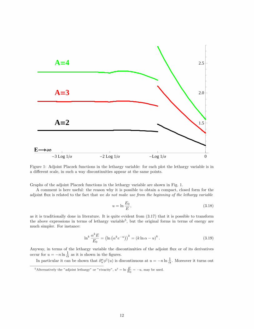
Figure 1: Adjoint Placzek functions in the lethargy variable: for each plot the lethargy variable is ina different scale, in such a way discontinuities appear at the same points.

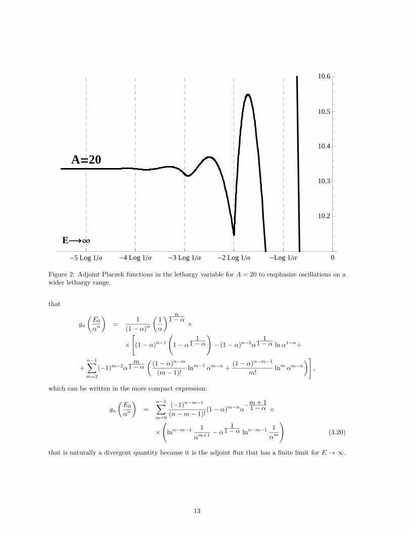
Graphs of the adjoint Placzek functions in the lethargy variable are shown in Fig. 1.A comment is here useful: the reason why it is possible to obtain a compact, closed form for the

adjoint flux is related to the fact that we do not make use from the beginning of the lethargy variable

u = lnE0

E, (3.18)

as it is traditionally done in literature. It is quite evident from (3.17) that it is possible to transformthe above expressions in terms of lethargy variable5, but the original forms in terms of energy aremuch simpler. For instance:

lnkαkE

E0=(ln(αke−u

))k= (k lnα− u)

k. (3.19)

Anyway, in terms of the lethargy variable the discontinuities of the adjoint flux or of its derivatives

occur for u = −n ln 1α as it is shown in the figures.

In particular it can be shown that ∂nuφ†(u) is discontinuous at u = −n ln 1

α . Moreover it turns out

5Alternatively the ”adjoint lethargy” or ”vivacity”, u† = ln EE0

= −u, may be used.

12

-5 Log 1Α -4 Log 1Α -3 Log 1Α -2 Log 1Α -Log 1Α 0

10.2

10.3

10.4

10.5

10.6

A=20

E¥

Figure 2: Adjoint Placzek functions in the lethargy variable for A = 20 to emphasize oscillations on awider lethargy range.

that

gn

(E0

αn

)=

1

(1− α)n

(1

α

) n1− α ×

×

[(1− α)n−1

(1− α

11− α

)− (1− α)n−2α

11− α lnα1−n+

+

n−1∑m=2

(−1)m−2αm

1− α(

(1− α)n−m

(m− 1)!lnm−1 αm−n +

(1− α)n−m−1

m!lnm αm−n

)],

which can be written in the more compact expression:

gn

(E0

αn

)=

n−1∑m=0

(−1)n−m−1

(n−m− 1)!(1− α)m−nα

−m+ 11− α ×

×

(lnn−m−1

1

αm+1 − α1

1− α lnn−m−11

αm

)(3.20)

that is naturally a divergent quantity because it is the adjoint flux that has a finite limit for E →∞.

13

This requires to divide by E0/αn, so yielding the adjoint flux values at the discontinuity points as:

φ†(E0

αn

)=

n−1∑m=0

(−1)n−m−1

(n−m− 1)!(1− α)m−nα

n−m+ 11− α ×

×

(lnn−m−1

1

αm+1 − α1

1− α lnn−m−11

αm

). (3.21)

This is a useful expression for approximate numerical evaluations, because it is stable for moderatevalues of n. However, the finiteness of the asymptotic limit for n→∞ is guaranteed only by the factorαn, being the sequence defined by (3.20) divergent.

4 Validation of the sampling procedure

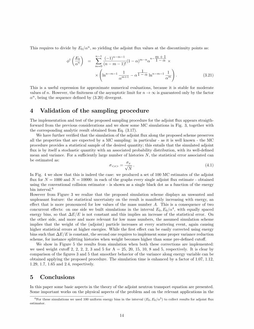
The implementation and test of the proposed sampling procedure for the adjoint flux appears straigth-forward from the previous considerations and we show some MC simulations in Fig. 3, together withthe corresponding analytic result obtained from Eq. (3.17).

We have further verified that the simulation of the adjoint flux along the proposed scheme preservesall the properties that are expected by a MC sampling: in particular - as it is well known - the MCprocedure provides a statistical sample of the desired quantity; this entails that the simulated adjointflux is by itself a stochastic quantity with an associated probability distribution, with its well-definedmean and variance. For a sufficiently large number of histories N , the statistical error associated canbe estimated as:

σ<x> =σx√N. (4.1)

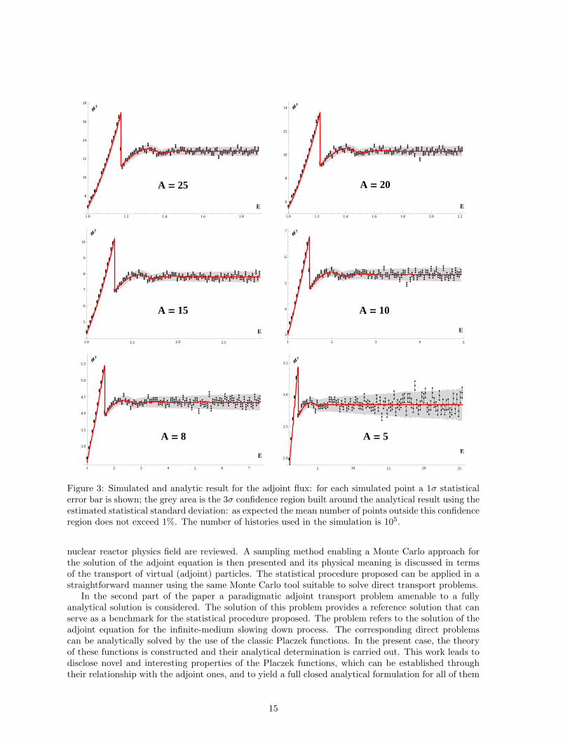
In Fig. 4 we show that this is indeed the case: we produced a set of 100 MC estimates of the adjointflux for N = 1000 and N = 10000: in each of the graphs every single adjoint flux estimate - obtainedusing the conventional collision estimator - is shown as a single black dot as a function of the energybin interval.6

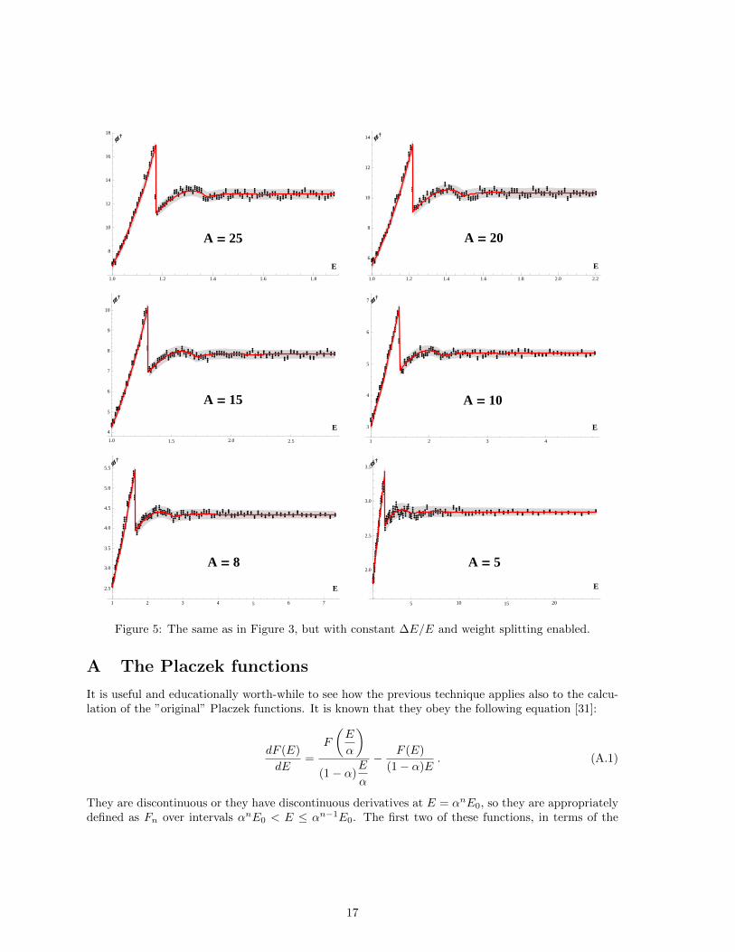
However from Figure 3 we realize that the proposed simulation scheme displays an unwanted andunpleasant feature: the statistical uncertainty on the result is manifestly increasing with energy, aneffect that is more pronounced for low values of the mass number A. This is a consequence of twoconcurrent effects: on one side we built simulations in the interval E0, E0/α

4, with equally spacedenergy bins, so that ∆E/E is not constant and this implies an increase of the statistical error. Onthe other side, and more and more relevant for low mass numbers, the assumed simulation schemeimplies that the weight of the (adjoint) particle increases at every scattering event, again causinghigher statistical errors at higher energies. While the first effect can be easily corrected using energybins such that ∆E/E is constant, the second one requires to implement some proper variance reductionscheme, for instance splitting histories when weight becomes higher than some pre-defined cutoff.

We show in Figure 5 the results from simulation when both these corrections are implemented:we used weight cutoff 2, 2, 2, 2, 3 and 5 for A = 25, 20, 15, 10, 8 and 5, respectively. It is clear bycomparison of the figures 3 and 5 that smoother behavior of the variance along energy variable can beobtained applying the proposed procedure. The simulation time is enhanced by a factor of 1.07, 1.12,1.29, 1.7, 1.65 and 2.4, respectively.

5 Conclusions

In this paper some basic aspects in the theory of the adjoint neutron transport equation are presented.Some important works on the physical aspects of the problem and on the relevant applications in the

6For these simulations we used 100 uniform energy bins in the interval (E0, E0/α5) to collect results for adjoint fluxestimator.

14

1.0 1.2 1.4 1.6 1.8

8

10

12

14

16

18

E

A = 25

Φ†

1.0 1.2 1.4 1.6 1.8 2.0 2.2

6

8

10

12

14

E

A = 20

Φ†

1.0 1.5 2.0 2.5

5

6

7

8

9

10

E

A = 15

Φ†

1 2 3 4 5

3

4

5

6

7

E

A = 10

Φ†

1 2 3 4 5 6 7

3.0

3.5

4.0

4.5

5.0

5.5

E

A = 8

Φ†

5 10 15 20 25

2.0

2.5

3.0

3.5

E

A = 5

Φ†

Figure 3: Simulated and analytic result for the adjoint flux: for each simulated point a 1σ statisticalerror bar is shown; the grey area is the 3σ confidence region built around the analytical result using theestimated statistical standard deviation: as expected the mean number of points outside this confidenceregion does not exceed 1%. The number of histories used in the simulation is 105.

nuclear reactor physics field are reviewed. A sampling method enabling a Monte Carlo approach forthe solution of the adjoint equation is then presented and its physical meaning is discussed in termsof the transport of virtual (adjoint) particles. The statistical procedure proposed can be applied in astraightforward manner using the same Monte Carlo tool suitable to solve direct transport problems.

In the second part of the paper a paradigmatic adjoint transport problem amenable to a fullyanalytical solution is considered. The solution of this problem provides a reference solution that canserve as a benchmark for the statistical procedure proposed. The problem refers to the solution of theadjoint equation for the infinite-medium slowing down process. The corresponding direct problemscan be analytically solved by the use of the classic Placzek functions. In the present case, the theoryof these functions is constructed and their analytical determination is carried out. This work leads todisclose novel and interesting properties of the Placzek functions, which can be established throughtheir relationship with the adjoint ones, and to yield a full closed analytical formulation for all of them

15

20 40 60 80 100bin ð2

4

6

8

10

12

Φ†

20 40 60 80 100bin ð2

4

6

8

10

12

Φ†

Figure 4: Distribution of adjoint flux samples for N = 1000 (on the left) and N = 10000 (on the right):larger (red) points represent the mean of the sampled flux estimates and the lower and upper limits ofrespective 3σ confidence interval. In this case A = 15.

(see Appendix A).The direct comparisons between the analytical results and those obtained by a Monte Carlo sim-

ulation allow to validate the suitability of the statistical approach proposed for the solution of theadjoint transport problem. The favorable comparison allows to conclude that the sampling procedurecan be successfully applied for the determination of the adjoint flux in neutron transport for reactorphysics applications.

16

1.0 1.2 1.4 1.6 1.8

8

10

12

14

16

18

E

A = 25

Φ†

1.0 1.2 1.4 1.6 1.8 2.0 2.2

6

8

10

12

14

E

A = 20

Φ†

1.0 1.5 2.0 2.5

4

5

6

7

8

9

10

E

A = 15

Φ†

1 2 3 4

3

4

5

6

7

E

A = 10

Φ†

1 2 3 4 5 6 7

2.5

3.0

3.5

4.0

4.5

5.0

5.5

E

A = 8

Φ†

5 10 15 20

2.0

2.5

3.0

3.5

E

A = 5

Φ†

Figure 5: The same as in Figure 3, but with constant ∆E/E and weight splitting enabled.

A The Placzek functions

It is useful and educationally worth-while to see how the previous technique applies also to the calcu-lation of the ”original” Placzek functions. It is known that they obey the following equation [31]:

dF (E)

dE=

F

(E

α

)(1− α)

E

α

− F (E)

(1− α)E. (A.1)

They are discontinuous or they have discontinuous derivatives at E = αnE0, so they are appropriatelydefined as Fn over intervals αnE0 < E ≤ αn−1E0. The first two of these functions, in terms of the

17

lethargy variable are given by (cfr. ibidem eqn. (8-50) and (8-55)):

F1(u) = S0

exp

[α

1− αu

]1− α

(A.2)

F2(u) = S0

1− α1

1− α1− α

exp

[α

1− αu

]− (A.3)

−S0α

α1− α

(1− α)2

(u− ln

1

α

)exp

[α

1− αu

], (A.4)

which can be translated into the energy variable as 7:

F1(E) =

S0

(E0

E

) α1− α

E(1− α)

F2(E) =

S0

(E0

E

) α1− α

E(1− α)2

[(1− α)

(1− α

11− α

)− (A.5)

− αα

1− α lnαE0

E

].

It is remarkable that in these two intervals (α2E0 < E < αE0 and αE0 < E < E0) the followingproperty holds:

E0Σs(E0)

S†0φ†1/2(E) = h1/2

(E

E0

),

EΣs(E)

S0φ1/2(E) = h1/2

(E0

E

). (A.6)

Let us suppose now that a function exists such that the previous relation hold over all the allowedenergy range, that is:

E0Σs(E0)

S†0φ†(E) = h

(E

E0

),

EΣs(E)

S0φ(E) = h

(E0

E

).

To prove the consistency of this hypothesis we can start from the equations for φ† and for ΣS(E)φ(E)and show that they imply the same equation for h(y)8: this is a necessary and sufficient condition

7It must be recalled that the definition given for the lethargy dependent collision density is such that

F (u)du = −F (E)dE,

which entailsF (u) = EF (E).

8In the case of ordinary first order differential equations to prove that two functions are identical it is sufficient toprove that they obey to the same equation and that they coincide in one point; this case is a little bit more complicatedbecause differential equations involved in the game are not ordinary ones, but first order differential-difference equationsin lethargy variable. In this case to fully specify a solution we must specify its values on the interval 1 < x < 1/α forthe argument of g(x).

18

because we have shown by inspection that (A.6) holds in the first two respective intervals of energy9.The equation to be satisfied by φ† for E > E0/α is

dφ†(E)

dE=

α

E(1− α)φ†(E)− α

E(1− α)φ†(αE)

and, multiplying byE0Σs(E0)

S†0,

dh

(E

E0

)dE

=α

E(1− α)h

(E

E0

)− α

E(1− α)h

(αE

E0

). (A.7)

On the other hand the equation satisfied by Fc(E) = Σs(E)φ(E) is [31] for E < αE0:

dFc(E)

dE=

1

E(1− α)

[Fc

(E

α

)− Fc(E)

]and then

d

dE

E

S0Fc(E) =

1

S0Fc(E) +

E

S0

dFcdE

=1

S0Fc(E) +

E

S0

1

E(1− α)

[Fc

(E

α

)− Fc(E)

]=

1

S0Fc(E)

[1− 1

1− α

]+

1

S0

1

(1− α)Fc

(E

α

)=

1

S0

1

(1− α)Fc

(E

α

)− 1

S0

α

1− αFc (E) ,

or

d

dEh

(E0

E

)=

α

E(1− α)h

(αE0

E

)− α

E(1− α)h

(E0

E

).

Now if we let y = E0E , we have:

− E0

E2

d

dyh (y) =

α

E(1− α)h (αy)− α

E(1− α)h (y) , (A.8)

ord

dyh (y) =

α

y(1− α)h (y)− α

y(1− α)h (αy) y > 1/α . (A.9)

On the other hand in (A.7) we can substitute z = E/E0 (and again we are constrained to z > 1/α),obtaining

dh (z)

dz=

α

z(1− α)h (z)− α

z(1− α)h (αz) . (A.10)

which is manifestly the same equation as (A.9):

9Effectively, the transformation EE0←→ E0

Emaps different energy intervals on a single one for the function h(x).

19

B Proof of equation (3.14)

Here we give the proof of eqn. (3.14):

g1(E) =1

1− α

(E

E0

) 11− α

g2(E) =1

(1− α)2

(E

E0

) 11− α

[(1− α)

(1− α

11− α

)− α

11− α ln

αE

E0

]

gn(E) =1

(1− α)n

(E

E0

) 11− α × (B.1)

×

[(1− α)n−1

(1− α

11− α

)− (1− α)n−2α

11− α ln

αE

E0+

+

n−1∑m=2

(−1)mαm

1− α(

(1− α)n−m

(m− 1)!lnm−1

αmE

E0+

(1− α)n−m−1

m!lnm

αmE

E0

)].

The term g2(E) can be found carrying out the following steps:

g2(E) =E

11− α

1− α

( α

E0

) 11− α ∫ E0/α

E0

g1(y)

ydy − α

11− α

∫ αE

E0

g1(y)

y1

1− α

dy

y

=

(E

E0

) 11− α

(1− α)2

( α

E0

) 11− α ∫ E0/α

E0

y1

1− α−1dy − α1

1− α∫ αE

E0

dy

y

=

(E

E0

) 11− α

(1− α)2

( α

E0

) 11− α

(1− α) y1

1− α∣∣∣∣∣E0/α

E0

− α1

1− α lnαE

E0

=

(E

E0

) 11− α

(1− α)2

[(1− α)

(1− α

11− α

)− α

11− α ln

αE

E0

].

Then we recognize that (B.1) implies for n > 2 an alternative recurrence relation for the functionsgn(E), namely:

gn(E) = gn−1(E) +(−1)n−1

(1− α)n

(E

E0

) 11− α

αn− 11− α × (B.2)

×(

(1− α)

(n− 2)!lnn−2

αn−1E

E0+

1

(n− 1)!lnn−1

αn−1E

E0

)≡ gn−1(E) + ∆n(E),

from which it is also immediate to conclude that

gn

(E0

αn−1

)= gn−1

(E0

αn−1

). (B.3)

20

Form (B.2), which is easily seen as perfectly equivalent to (B.1)10, is simpler to use to obtain a proofby mathematical induction. Suppose in fact that the equation defining gn:

dgn(E)

dE= − 1

1− αgn−1(αE)

E+

1

1− αgn(E)

E(B.4)

holds for some value of n > 2. Next insert (B.2) for gn+1(E); we have

dgn+1(E)

dE=

dgn(E)

dE+d∆n+1(E)

dE.

We must verify that this expression is equal to the following one:

− 1

1− αgn(αE)

E+

1

1− αgn+1(E)

E

− 1

1− αgn−1(αE) + ∆n(αE)

E+

1

1− αgn(E) + ∆n+1(E)

E,

that is to say that ∆n(E) itself satisfies the same equation as the gn’s; however, by definition thefollowing equality holds:

d∆n(E)

dE=

∆n(E)

E(1− α)+

(−1)n−1

(1− α)n

(E

E0

) 11− α

αn− 11− α d

dE

(· · ·).

Therefore, to prove our thesis we must simply show that

−∆n−1(αE)

(1− α)E=

(−1)n−1

(1− α)n

(E

E0

) 11− α

αn− 11− α ×

× d

dE

((1− α)

(n− 2)!lnn−2

αn−1E

E0+

1

(n− 1)!lnn−1

αn−1E

E0

)

=(−1)n−1

(1− α)n

(αE

E0

) 11− α

αn− 21− α 1

E×(

(1− α)

(n− 3)!lnn−3

αn−1E

E0+

1

(n− 2)!lnn−2

αn−1E

E0

),

or

∆n−1(αE) =(−1)n−2

(1− α)n−1

(αE

E0

) 11− α

αn− 21− α ×

×(

(1− α)

(n− 3)!lnn−3

αn−2(αE)

E0+

1

(n− 2)!lnn−2

αn−2(αE)

E0

),

which, being

∆n(E) =(−1)n−1

(1− α)n

(E

E0

) 11− α

αn− 11− α ×

×(

(1− α)

(n− 2)!lnn−2

αn−1E

E0+

1

(n− 1)!lnn−1

αn−1E

E0

),

is trivially verified. QED

10Because one simply makes explicit the last term in the sum and simplifies an overall factor 1 − α in the remainingterms, so reproducing the same form (B.1), with n replaced by n− 1.

21

References

[1] A. M. Weinberg and E. P. Wigner, The Physical Theory of Neutron Chain Reactors. Chicago, IL:The University of Chicago Press, 1958.

[2] L. N. Ussachoff, “Equation for the importanc of neutrons, reactor kinetics and the theory ofperturbations,” in International Conference on the Peaceful Uses of Atomic Energy, (Geneva),1955.

[3] M. A. Robkin and M. J. Clark, “Integral reactor theory: Orthogonality and importance,” NuclearScience and Engineering, vol. 8, pp. 437–442, 1960.

[4] I. Pazsit and V. Dykin, “The dynamic adjoint as a Green’s function,” Annals of Nuclear Energy,vol. 86, pp. 29–34, 2015.

[5] J. Lewins, Importance, the Adjoint Function: The Physical Basis of Variational and PerturbationTheory in Transport and Diffusion Problems. Elsevier Science & Technology, 1965.

[6] A. Gandini, “A generalized perturbation method for bi-linear functionals of the real and adjointneutron fluxes,” Journal of Nuclear Energy, vol. 21, pp. 755–765, 1967.

[7] A. Gandini, “Generalized perturbation theory (gpt) methods. a heuristic approach,” in Advancesin Nuclear Science and Technology (J. Lewins and M. Becker, eds.), ch. 19, New York: PlenumPublishing Corporation, 1987.

[8] A. Gandini, M. Salvatores, and L. Tondinelli, “New developments in generalized perturbationmethods in the nuclide field,” Nuclear Science and Engineering, vol. 62, pp. 339–345, 1977.

[9] S. Dulla, F. Cadinu, and P. Ravetto, “Neutron importance in source-driven systems,” in Interna-tional Topical Meeting on Mathematics and Computation, Supercomputing, Reactor Physics andBiological Applications, (Avignon), 2005.

[10] A. F. Henry, “The application of reactor kinetics to the analysis of experiments,” Nuclear Scienceand Engineering, vol. 3, pp. 52–70, 1958.

[11] S. Dulla, E. Mund, and P. Ravetto, “The quasi-static method revisited,” Progress in NuclearEnergy, vol. 908-920, pp. 52–70, 2008.

[12] H. Abdel-Khalik, “Adjoint-based sensitivity analysis for multi-component models,” Nuclear En-gineering and Design, vol. 245, pp. 49–54, 2012.

[13] H. Rief, “Generalized Monte Carlo perturbation algorithms for correlated sampling and a second-order taylor series approach,” Annals of Nuclear Energy, vol. 11, pp. 455–476, 1984.

[14] H. Rief, “Review of Monte Carlo techniques for analyzing reactor perturbations,” Annals of Nu-clear Energy, vol. 11, pp. 455–476, 1984.

[15] M. Aufiero, A. Bidaud, M. Hursin, J. Leppanen, G. Palmiotti, S. Pelloni, P. Rubiolo, A collisionhistory-based approach to sensitivity/perturbation calculations in the continuous energy MonteCarlo code SERPENT, Annals of Nuclear Energy, 85, 245-258, 2015

[16] B. Kiedrowski, B. Brown, and W. Wilson, “Calculating kinetic parameters and reactivity changeswith continuous energy Monte Carlo,” in International Conference PHYSOR-2010, (Pittsburgh),2010.

[17] J. Leppanen, M. Aufiero, E. Fridman, R. Rachamin, S. van der Marck Calculation of effectivepoint kinetics parameters in the Serpent 2 Monte Carlo code, Annals of Nuclear Energy, 65,272-279, 2014

22

[18] Computing adjoint-weighted kinetics parameters in Tripoli-4/E by the Iterated Fission Probabilitymethod, Annals of Nuclear Energy, 85, 17-26, 2015 G. Truchet, P. Leconte, A. Santamarina, E.Brun, F. Damian, A. Zoia

[19] A. Dubi and S. Gerstl, “Application of biasing techniques to the contributon monte carlo method,”Nuclear Science and Engineering, vol. 76, pp. 198–217, 1980.

[20] J. Densmore and E. W. Larsen, “Variational variance reduction for particle transport eigenvaluecalculations using Monte Carlo adjoint simulation,” Journal of Computational Physics, vol. 192,pp. 387–405, 2003.

[21] L. Carter, MCNA, a Computer Program to Solve the Adjoint Neutron Transport Equation byCoupled Sampling with the Monte Carlo Method. Los Alamos National Laboratory, Los Alamos,NM: LA-4488, 1971.

[22] J. E. Hoogenboom, “Methodology of continuous energy adjoint monte carlo for neutron photonand coupled neutron photon transport,” Nuclear Science and Engineering, vol. 143, pp. 99–120,2003.

[23] S. A. H. Feghhi, M. Shahriari, and H. Afarideh, “Calculation of neutron importance function infissionable assemblies using Monte Carlo method,” Annals of Nuclear Energy, vol. 34, pp. 514–520,2007.

[24] C. M. Diop, O. Petit, C. Jouanne, and M. Coste-Delclaux, “Adjoint Monte Carlo neutron transportusing cross section probability table representation,” Annals of Nuclear Energy, vol. 37, pp. 1186–1196, 2010.

[25] D. C. Irving, “The adjoint boltzmann equation and its simulation by monte carlo,” NuclearEngineering and Design, vol. 15, pp. 273–292, 1971.

[26] A. De Matteis, “Phenomenological interpretation of the adjoint neutron transport equation,”Meccanica, vol. 3, pp. 162–164, 1974.

[27] A. De Matteis, R. Simonini, “A new Monte Carlo approach to the adjoint Boltzmann equation”,Nuclear Science and Engineering, vol. 65, pp. 93-105, 1978.

[28] B. Eriksson, C. Johansson, M. Leimdorfer, M. H. Kalos, ”Monte Carlo Integration of the AdjointNeutron Transport Equation”, Nuclear Science and Engineering, vol. 37, pages 410-422, 1969.

[29] B. Ganapol, Analytical Benchmarks for Nuclear Engineering Applications, Case Studies in Neu-tron Transport Theory. NEA Data Bank, Paris: NEA/DB/DOC(2008)1, 6292, 2008.

[30] G. Placzek, “On the theory of the slowing down of neutrons in heavy substances,” Physical Review,vol. 69, pp. 423–438, 1946.

[31] J. J. Duderstadt and W. R. Martin, Transport Theory. New York: Wiley, 1979.

23