Embed Size (px)
Citation preview

111
CHALLENGEThe increased employment of mothers outside the home has led to a steep rise in the use ofchild care over the past several decades. In the United States, nearly seven out of ten moth-ers work today—more than twice the rate in 1970. Eight out of ten employed mothers with chil-dren under age six are likely to have some form of nonparental child-care arrangement. Six outof ten children under the age of six are in child care, as are 45% of children underage one.
Child care is a major burden for the poor, and the expense may prevent poormothers from working. Paying for child care for children under the age of fiveabsorbed 25% of the earnings for families with annual incomes under $14,400, butonly 6% for families with incomes of $54,000 or more. Government child-care sub-sidies increase the probability that a single mother will work at a standard job by7% (Tekin, 2007). As one would expect, the subsidies have larger impacts on wel-fare recipients than on wealthier mothers.
In large part to help poor families obtain child care so that the parents couldwork, the U.S. Child Care and Development Fund (CCDF) provided $7 billion tostates in 2009. Child-care programs vary substantially across states in their gen-erosity and in the form of the subsidy.1
Most states provide an ad valorem or a specific subsidy (see Chapter 3) tolower the hourly rate that a poor family pays for child care. Rather than subsidizingthe price of child care, the government could provide an unrestricted lump-sumpayment that could be spent on child care or on all other goods, such as food andhousing. Canada provides such lump-sum payments.
For a given government expenditure, does a price subsidy or lump-sum subsidyprovide greater benefit to recipients? Which increases the demand for child-careservices by more? Which inflicts less cost on other consumers of child care?
5ApplyingConsumer Theory
We can answer these questions using consumer theory. We can also use consumertheory to derive demand curves, to analyze the effects of providing cost-of-livingadjustments to deal with inflation, and to derive labor supply curves.
We start by using consumer theory to show how to determine the shape of ademand curve for a good by varying the price of a good, holding other prices andincome constant. Firms use information about the shape of demand curves whensetting prices. Governments apply this information in predicting the impact of poli-cies such as taxes and price controls.
I have enough money to last me the rest of my life, unless I buy something.—Jackie Mason
Per-Hour VersusLump-Sum Child-
Care Subsidies
5
1For example, for a family with two children to be eligible for a subsidy in 2009, the family’s max-imum income was $4,515 in California but $2,863 in Louisiana. The maximum subsidy for a tod-dler was $254 per week in California and $92.50 per week in Louisiana. The family’s fee for childcare ranged between 20% and 60% of the cost of care in Louisiana, between 2% and 10% in Maine,and between $0 and $495 per month in Minnesota.
5.1 Deriving Demand CurvesWe use consumer theory to show by how much the quantity demanded of a goodfalls as its price rises. An individual chooses an optimal bundle of goods by pickingthe point on the highest indifference curve that touches the budget line (Chapter 4).When a price changes, the budget constraint the consumer faces shifts, so the con-sumer chooses a new optimal bundle. By varying one price and holding other pricesand income constant, we determine how the quantity demanded changes as the pricechanges, which is the information we need to draw the demand curve. After deriv-ing an individual’s demand curve, we show the relationship between consumer
We then use consumer theory to show how an increase in income causes thedemand curve to shift. Firms use information about the relationship betweenincome and demand to predict which less-developed countries will substantiallyincrease their demand for the firms’ products.
Next, we show that an increase in the price of a good has two effects on demand.First, consumers would buy less of the now relatively more expensive good even ifthey were compensated with cash for the price increase. Second, consumers’incomes can’t buy as much as before because of the higher price, so consumers buyless of at least some goods.
We use this analysis of these two demand effects of a price increase to show whythe government’s measure of inflation, the Consumer Price Index (CPI), overesti-mates the amount of inflation. Because of this bias in the CPI, some people gain andsome lose from contracts that adjust payment on the basis of the government’s infla-tion index. If you signed a long-term lease for an apartment in which your rent pay-ments increase over time in proportion to the change in the CPI, you lose and yourlandlord gains from this bias.
Finally, we show how we can use the consumer theory of demand to determinean individual’s labor supply curve. Knowing the shape of workers’ labor supplycurves is important in analyzing the effect of income tax rates on work and on taxcollections. Many politicians, including Presidents John F. Kennedy, Ronald Reagan,and George W. Bush, have argued that if the income tax rates were cut, workerswould work so many more hours that tax revenues would increase. If so, everyonecould be made better off by a tax cut. If not, the deficit could grow to record levels.Economists use empirical studies based on consumer theory to predict the effect ofthe tax rate cut on tax collections, as we discuss at the end of this chapter.
112 CHAPTER 5 Applying Consumer Theory
1. Deriving Demand Curves. We use consumer theory to derive demand curves, showinghow a change in price causes a shift along a demand curve.
2. How Changes in Income Shift Demand Curves. We use consumer theory to determinehow a demand curve shifts because of a change in income.
3. Effects of a Price Change. A change in price has two effects on demand, one having todo with a change in relative prices and the other concerning a change in the consumer’sopportunities.
4. Cost-of-Living Adjustments. Using this analysis of the two effects of price changes, weshow that the CPI overestimates the rate of inflation.
5. Deriving Labor Supply Curves. Using consumer theory to derive the demand curve forleisure, we can derive workers’ labor supply curves and use them to determine how areduction in the income tax rate affects labor supply and tax revenues.
In this chapter, weexamine five maintopics
1135.1 Deriving Demand Curves
4.3
5.2
12.0
2.8
12.0
6.0
4.0
26.70 44.5 58.9
L1 (pb = $12)
p b, $
per
uni
t
L2 (pb = $6) L3 (pb = $4)
26.70 44.5 58.9
e3
e2
e1
E3
E2
E1
I1
I2
I3
Beer, Gallons per year
Beer, Gallons per year
D1, Demand for beer
Price-consumption curve
Win
e, G
allo
ns p
er y
ear
(a) Indifference Curves and Budget Constraints
(b) Demand Curve
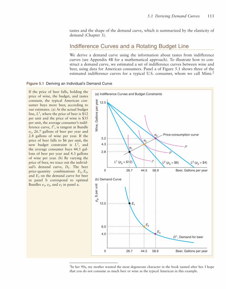
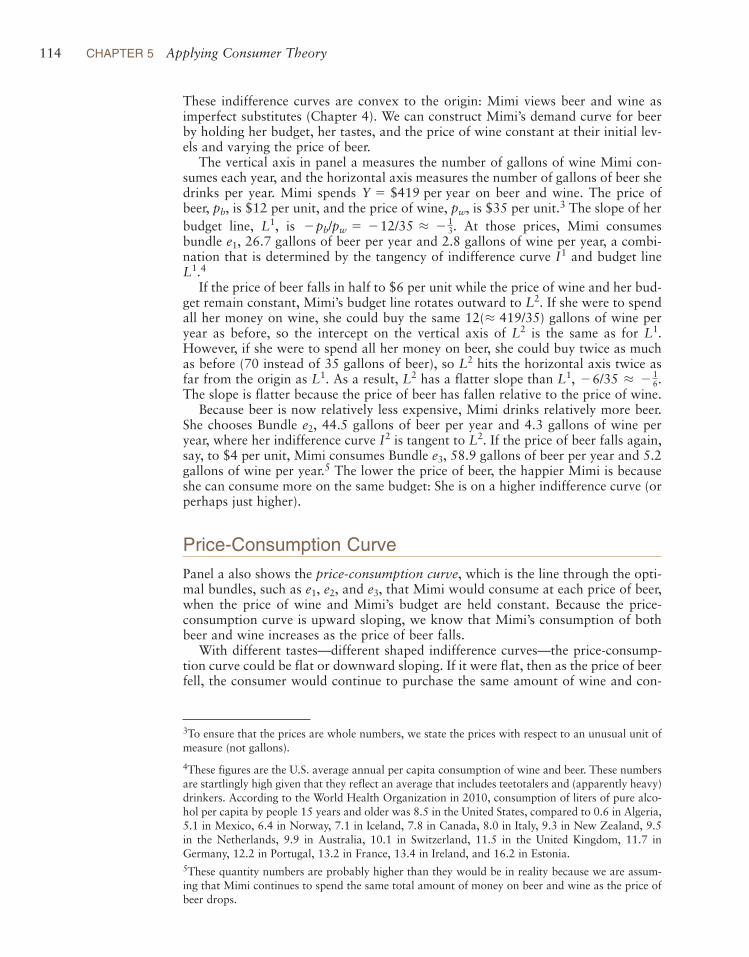
Figure 5.1 Deriving an Individual’s Demand Curve
If the price of beer falls, holding theprice of wine, the budget, and tastesconstant, the typical American con-sumer buys more beer, according toour estimates. (a) At the actual budgetline, where the price of beer is $12per unit and the price of wine is $35per unit, the average consumer’s indif-ference curve, is tangent at Bundle
26.7 gallons of beer per year and2.8 gallons of wine per year. If theprice of beer falls to $6 per unit, thenew budget constraint is and the average consumer buys 44.5 gal-lons of beer per year and 4.3 gallonsof wine per year. (b) By varying theprice of beer, we trace out the individ-ual’s demand curve, The beerprice-quantity combinations and on the demand curve for beerin panel b correspond to optimalBundles and in panel a.e3e1, e2,
E3
E1, E2,D1.
L2,
e1,I1,
L1,
tastes and the shape of the demand curve, which is summarized by the elasticity ofdemand (Chapter 3).
Indifference Curves and a Rotating Budget LineWe derive a demand curve using the information about tastes from indifferencecurves (see Appendix 4B for a mathematical approach). To illustrate how to con-struct a demand curve, we estimated a set of indifference curves between wine andbeer, using data for American consumers. Panel a of Figure 5.1 shows three of theestimated indifference curves for a typical U.S. consumer, whom we call Mimi.2
2In her 90s, my mother wanted the most degenerate character in the book named after her. I hopethat you do not consume as much beer or wine as the typical American in this example.
114 CHAPTER 5 Applying Consumer Theory
These indifference curves are convex to the origin: Mimi views beer and wine asimperfect substitutes (Chapter 4). We can construct Mimi’s demand curve for beerby holding her budget, her tastes, and the price of wine constant at their initial lev-els and varying the price of beer.
The vertical axis in panel a measures the number of gallons of wine Mimi con-sumes each year, and the horizontal axis measures the number of gallons of beer shedrinks per year. Mimi spends on beer and wine. The price ofbeer, is $12 per unit, and the price of wine, is $35 per unit.3 The slope of herbudget line, is At those prices, Mimi consumes bundle 26.7 gallons of beer per year and 2.8 gallons of wine per year, a combi-nation that is determined by the tangency of indifference curve and budget line
4
If the price of beer falls in half to $6 per unit while the price of wine and her bud-get remain constant, Mimi’s budget line rotates outward to If she were to spendall her money on wine, she could buy the same gallons of wine peryear as before, so the intercept on the vertical axis of is the same as for However, if she were to spend all her money on beer, she could buy twice as muchas before (70 instead of 35 gallons of beer), so hits the horizontal axis twice asfar from the origin as As a result, has a flatter slope than The slope is flatter because the price of beer has fallen relative to the price of wine.
Because beer is now relatively less expensive, Mimi drinks relatively more beer.She chooses Bundle 44.5 gallons of beer per year and 4.3 gallons of wine peryear, where her indifference curve is tangent to If the price of beer falls again,say, to $4 per unit, Mimi consumes Bundle 58.9 gallons of beer per year and 5.2gallons of wine per year.5 The lower the price of beer, the happier Mimi is becauseshe can consume more on the same budget: She is on a higher indifference curve (orperhaps just higher).
Price-Consumption CurvePanel a also shows the price-consumption curve, which is the line through the opti-mal bundles, such as and that Mimi would consume at each price of beer,when the price of wine and Mimi’s budget are held constant. Because the price-consumption curve is upward sloping, we know that Mimi’s consumption of bothbeer and wine increases as the price of beer falls.
With different tastes—different shaped indifference curves—the price-consump-tion curve could be flat or downward sloping. If it were flat, then as the price of beerfell, the consumer would continue to purchase the same amount of wine and con-
e3,e1, e2,
e3,L2.I2
e2,
L1, !6/35 L !16.L2L1.
L2
L1.L212(L 419/35)
L2.
L1.I1
e1,!pb/pw = !12/35 L !1
3.L1,pw,pb,
Y = $419 per year
4These figures are the U.S. average annual per capita consumption of wine and beer. These numbersare startlingly high given that they reflect an average that includes teetotalers and (apparently heavy)drinkers. According to the World Health Organization in 2010, consumption of liters of pure alco-hol per capita by people 15 years and older was 8.5 in the United States, compared to 0.6 in Algeria,5.1 in Mexico, 6.4 in Norway, 7.1 in Iceland, 7.8 in Canada, 8.0 in Italy, 9.3 in New Zealand, 9.5in the Netherlands, 9.9 in Australia, 10.1 in Switzerland, 11.5 in the United Kingdom, 11.7 inGermany, 12.2 in Portugal, 13.2 in France, 13.4 in Ireland, and 16.2 in Estonia.5These quantity numbers are probably higher than they would be in reality because we are assum-ing that Mimi continues to spend the same total amount of money on beer and wine as the price ofbeer drops.
3To ensure that the prices are whole numbers, we state the prices with respect to an unusual unit ofmeasure (not gallons).

I phoned my dad to tell him I had stopped smoking. He called me a quitter.—Steven Pearl
Tobacco use, one of the biggest public health threats the world has ever faced,killed 100 million people in the twentieth century. In 2010, the U.S. Center forDisease Control (CDC) reported that cigarette smoking and secondhandsmoke are responsible for nearly one of every five deaths each year in theUnited States. Half of all smokers die of tobacco-related causes; worldwide,tobacco kills 5.4 million people a year. Of the more than one billion smokersin the world, more than 80% live in low- and middle-income countries.
One way to get people to quit smoking is to raise the relative price oftobacco to that of other goods (thereby changing the slope of the budget con-straints that individuals face). In poorer countries, smokers are giving upcigarettes to buy cell phones. As cell phones have recently become affordablein many poorer countries, the price ratio of cell phones to tobacco has fallensubstantially. To pay for mobile phones, consumers reduce their expenditureson other goods, including tobacco.
According to Labonne and Chase (2008), in 2003, before cell phones werecommon, 42% of households in the Philippine villages they studied usedtobacco, and 2% of total village income was spent on tobacco. After the priceof cell phones fell, ownership of the phones quadrupled from 2003 to 2006. Asconsumers spent more on mobile phones, tobacco use fell by a third in house-holds in which at least one member had smoked (so that consumption fell bya fifth for the entire population). That is, if we put cell phones on the horizon-tal axis and tobacco on the vertical axis and lower the price of cell phones, theprice-consumption curve is downward sloping (unlike in Figure 5.1—seeQuestion 1 at the end of the chapter).
Cigarette taxes are often used to increase the price of cigarettes relative toother goods. At least 163 countries tax cigarettes to raise tax revenue and todiscourage socially harmful behavior. Lower-income and younger populationsare more likely than others to quit smoking if the price rises. Colman andRemler (2008) estimated that price elasticities of demand for cigarettes amonglow-, middle-, and high-income groups are and respec-tively. Several economic studies estimated that the price elasticity of demand isbetween and for the general U.S. population and between and for children. When the after-tax price of cigarettes in Canadaincreased 158% from 1979 to 1991 (after adjusting for inflation), teenagesmoking dropped by 61% and overall smoking fell by 38%.
But what happens to those who continue to smoke heavily? To pay for theirnow more expensive habit, they have to reduce their expenditures on othergoods, such as housing and food. Busch et al. (2004) found that a 10%increase in the price of cigarettes causes poor smoking families to cut back oncigarettes by 9%, alcohol and transportation by 11%, food by 17%, andhealth care by 12%. Among the poor, smoking families allocate 36% of theirexpenditures to housing compared to 40% for nonsmokers. Thus, to continueto smoke, these people cut back on many basic goods. That is, if we puttobacco on the horizontal axis and all other goods on the vertical axis, theprice-consumption curve is upward sloping, so that as the price of tobaccorises, the consumer buys less of both tobacco and all other goods.
!0.7!0.6!0.6!0.3
!0.20,!0.37, !0.35,
1155.1 Deriving Demand Curves
See Question 1 andProblems 33 and 34.
sume more beer. If the price-consumption curve were downward sloping, the indi-vidual would consume more beer and less wine as the price of beer fell.
APPLICATION
Quitting Smoking
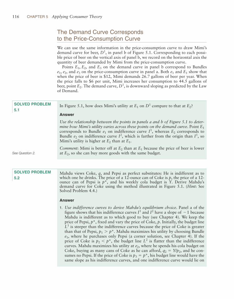
Mahdu views Coke, q, and Pepsi as perfect substitutes: He is indifferent as towhich one he drinks. The price of a 12-ounce can of Coke is p, the price of a 12-ounce can of Pepsi is and his weekly cola budget is Y. Derive Mahdu’sdemand curve for Coke using the method illustrated in Figure 5.1. (Hint: SeeSolved Problem 4.4.)
Answer
1. Use indifference curves to derive Mahdu’s equilibrium choice. Panel a of thefigure shows that his indifference curves and have a slope of becauseMahdu is indifferent as to which good to buy (see Chapter 4). We keep theprice of Pepsi, fixed and vary the price of Coke, p. Initially, the budget line
is steeper than the indifference curves because the price of Coke is greaterthan that of Pepsi, Mahdu maximizes his utility by choosing Bundle
where he purchases only Pepsi (a corner solution, see Chapter 4). If theprice of Coke is the budget line is flatter than the indifferencecurves. Mahdu maximizes his utility at where he spends his cola budget onCoke, buying as many cans of Coke as he can afford, and he con-sumes no Pepsi. If the price of Coke is his budget line would have thesame slope as his indifference curves, and one indifference curve would lie on
p3 = p*,q2 = Y/p2,
e2,L2p2 6 p*,
e1,p1 7 p*.
L1p*,
!1I2I1
p*,
In Figure 5.1, how does Mimi’s utility at on compare to that at
Answer
Use the relationship between the points in panels a and b of Figure 5.1 to deter-mine how Mimi’s utility varies across these points on the demand curve. Point corresponds to Bundle on indifference curve whereas corresponds toBundle on indifference curve which is farther from the origin than soMimi’s utility is higher at than at
Comment: Mimi is better off at than at because the price of beer is lowerat so she can buy more goods with the same budget.E2,
E1E2
E1.E2
I1,I2,e2
E2I1,e1
E1
E2?D1E1
116 CHAPTER 5 Applying Consumer Theory
The Demand Curve Corresponds to the Price-Consumption CurveWe can use the same information in the price-consumption curve to draw Mimi’sdemand curve for beer, in panel b of Figure 5.1. Corresponding to each possi-ble price of beer on the vertical axis of panel b, we record on the horizontal axis thequantity of beer demanded by Mimi from the price-consumption curve.
Points and on the demand curve in panel b correspond to Bundlesand on the price-consumption curve in panel a. Both and show that
when the price of beer is $12, Mimi demands 26.7 gallons of beer per year. Whenthe price falls to $6 per unit, Mimi increases her consumption to 44.5 gallons ofbeer, point The demand curve, is downward sloping as predicted by the Lawof Demand.
D1,E2.
E1e1e3e1, e2,E3E1, E2,
D1,
SOLVED PROBLEM 5.1
See Question 2.
SOLVED PROBLEM 5.2

1175.1 Deriving Demand Curves
See Question 3.
top of the budget line. Consequently, he would be indifferent between buyingany quantity of q between 0 and (and his total purchases of Cokeand Pepsi would add to ).
2. Use the information in panel a to draw his Coke demand curve. Panel b showsMahdu’s demand curve for Coke, q, for a given price of Pepsi, and Y.When the price of Coke is above his demand curve lies on the vertical axis,where he demands zero units of Coke, such as point in panel b, which cor-responds to in panel a. If the prices are equal, he buys any amount of Cokeup to a maximum of If the price of Coke is he buys
units at point which corresponds to in panel a. When the price ofCoke is less than that of Pepsi, the Coke demand curve asymptoticallyapproaches the horizontal axis as the price of Coke approaches zero.
e2E2,Y/p2
p2 6 p*,Y/p3 = Y/p*.e1
E1
p*,p*,
Y/p3 = Y/p*Y/p3 = Y/p*
Coke demand curve
(a) Indifference Curves and Budget Constraints
(b) Coke Demand Curve
p, Do
llars
per c
an
q, Cans of Coke per week
p*
Y/p3 = Y/p*
q, Cans ofCoke per week
I2
I1
Cans
of P
epsi
per w
eek
L2
L1
e1
e2
E1
E2
q2 = Y/p2q1 = 0
q2 = Y/p2q1 = 0
p1
p2

118 CHAPTER 5 Applying Consumer Theory
5.2 How Changes in Income Shift Demand CurvesTo trace out the demand curve, we looked at how an increase in the good’s price—holding income, tastes, and other prices constant—causes a downward movementalong the demand curve. Now we examine how an increase in income, when allprices are held constant, causes a shift of the demand curve.
Businesses routinely use information on the relationship between income and thequantity demanded. For example, in deciding where to market its products,Whirlpool wants to know which countries are likely to spend a relatively large per-centage of any extra income on refrigerators and washing machines.
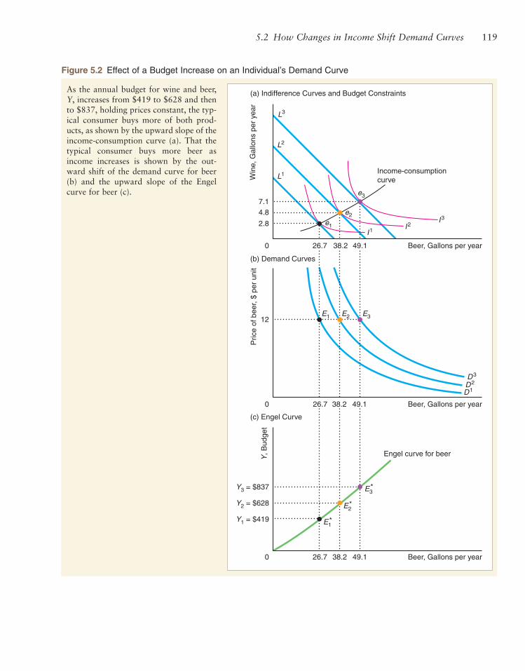
Effects of a Rise in IncomeWe illustrate the relationship between the quantity demanded and income by exam-ining how Mimi’s behavior changes when her income rises while the prices of beerand wine remain constant. Figure 5.2 shows three ways of looking at the relation-ship between income and the quantity demanded. All three diagrams have the samehorizontal axis: the quantity of beer consumed per year. In the consumer theory dia-gram, panel a, the vertical axis is the quantity of wine consumed per year. In thedemand curve diagram, panel b, the vertical axis is the price of beer per unit. Finally,in panel c, which shows the relationship between income and quantity directly, thevertical axis is Mimi’s budget, Y.
A rise in Mimi’s income causes the budget constraint to shift outward in panel a,which increases Mimi’s opportunities. Her budget constraint at her originalincome, is tangent to her indifference curve at
As before, Mimi’s demand curve for beer is in panel b. Point on whichcorresponds to point in panel a, shows how much beer, 26.7 gallons per year,Mimi consumes when the price of beer is $12 per unit (and the price of wine is $35per unit).
Now suppose that Mimi’s beer and wine budget, Y, increases by roughly 50% to$628 per year. Her new budget line, in panel a, is farther from the origin but par-allel to her original budget constraint, because the prices of beer and wine areunchanged. Given this larger budget, Mimi chooses Bundle The increase in herincome causes her demand curve to shift to in panel b. Holding Y at $628, wecan derive by varying the price of beer, in the same way as we derived inFigure 5.1. When the price of beer is $12 per unit, she buys 38.2 gallons of beer peryear, on Similarly, if Mimi’s income increases to $837 per year, her demandcurve shifts to
The income-consumption curve through Bundles and in panel a showshow Mimi’s consumption of beer and wine increases as her income rises. As Mimi’sincome goes up, her consumption of both wine and beer increases.
We can show the relationship between the quantity demanded and incomedirectly rather than by shifting demand curves to illustrate the effect. In panel c, weplot an Engel curve, which shows the relationship between the quantity demandedof a single good and income, holding prices constant. Income is on the vertical axis,and the quantity of beer demanded is on the horizontal axis. On Mimi’s Engel curvefor beer, points and correspond to points and in panel b andto and in panel a.e3e1, e2,
E3E1, E2,E3*E1
*, E2*,
e3e1, e2,D3.
D2.E2
D1D2D2
e2.L1,
L2
e1
D1,E1D1e1.I1Y = $419,
L1
Engel curvethe relationship betweenthe quantity demanded ofa single good andincome, holding pricesconstant
1195.2 How Changes in Income Shift Demand Curves
Win
e, G
allo
ns p
er y
ear
Income-consumptioncurve
Engel curve for beer
0
2.84.87.1
49.138.226.7 Beer, Gallons per year
0
12
0
49.138.226.7 Beer, Gallons per year
49.138.226.7 Beer, Gallons per year
I2I3
I1
(a) Indifference Curves and Budget Constraints
Pric
e of
bee
r, $
per
unit
(b) Demand CurvesY
, Bud
get
(c) Engel Curve
e2
e3
E3E1 E2
Y1 = $419
Y2 = $628
Y3 = $837
L3
L2
L1
e1
D1D2D3
E1
E2
E3
*
*
*
Figure 5.2 Effect of a Budget Increase on an Individual’s Demand Curve
As the annual budget for wine and beer,Y, increases from $419 to $628 and thento $837, holding prices constant, the typ-ical consumer buys more of both prod-ucts, as shown by the upward slope of theincome-consumption curve (a). That thetypical consumer buys more beer asincome increases is shown by the out-ward shift of the demand curve for beer(b) and the upward slope of the Engelcurve for beer (c).
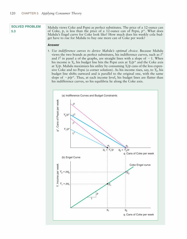
Mahdu views Coke and Pepsi as perfect substitutes. The price of a 12-ounce canof Coke, p, is less than the price of a 12-ounce can of Pepsi, What doesMahdu’s Engel curve for Coke look like? How much does his weekly cola bud-get have to rise for Mahdu to buy one more can of Coke per week?
Answer
1. Use indifference curves to derive Mahdu’s optimal choice. Because Mahduviews the two brands as perfect substitutes, his indifference curves, such as and in panel a of the graphs, are straight lines with a slope of Whenhis income is his budget line hits the Pepsi axis at and the Coke axisat Mahdu maximizes his utility by consuming cans of the less expen-sive Coke and no Pepsi (a corner solution). As his income rises, say, to hisbudget line shifts outward and is parallel to the original one, with the sameslope of Thus, at each income level, his budget lines are flatter thanhis indifference curves, so his equilibria lie along the Coke axis.
!p/p*.
Y2,Y1/pY1/p.
Y1/p*Y1,!1.I2
I1
p*.
120 CHAPTER 5 Applying Consumer Theory
SOLVED PROBLEM 5.3
Y2/p*
Y1/p*
Y1 = pq1
Y2 = pq2
q1 = Y1/p q2 = Y2/p
Y, In
come
per w
eek
e2e1
E2
E1
p
1
q, Cans of Coke per week
q1 q2q, Cans of Coke per week
q*, C
ans o
f Pep
si pe
r wee
k
(a) Indifference Curves and Budget Constraints
(b) Engel Curve
Coke Engel curve
L1
L2
I1
I2

1215.2 How Changes in Income Shift Demand Curves
2. Use the first figure to derive his Engel curve. Because his entire budget, Y, goesto buying Coke, Mahdu buys cans of Coke. This expression, whichshows the relationship between his income and the quantity of Coke he buys,is Mahdu’s Engel curve for Coke. The points and on the Engel curve inpanel b correspond to and in panel a. We can rewrite this expression forhis Engel curve as This relationship is drawn in panel b as a straightline with a slope of p. As q increases by one can (“run”), Y increases by p(“rise”). Because all his cola budget goes to buying Coke, his income needs torise by only p for him to buy one more can of Coke per week.
Y = pq.e2e1
E2E1
q = Y/p
See Questions 4 and 5 andProblem 35.
Consumer Theory and Income ElasticitiesIncome elasticities tell us how much the quantity demanded changes as incomeincreases. We can use income elasticities to summarize the shape of the Engel curve,the shape of the income-consumption curve, or the movement of the demand curveswhen income increases. For example, firms use income elasticities to predict theimpact of income taxes on consumption. We first discuss the definition of incomeelasticities and then show how they are related to the income-consumption curve.
Income Elasticities We defined the income elasticity of demand in Chapter 3 as
where is the Greek letter xi. Mimi’s income elasticity of beer, is 0.88, and thatof wine, is 1.38 (based on our estimates for the average American consumer).When her income goes up by 1%, she consumes 0.88% more beer and 1.38% morewine. Thus, according to these estimates, as income falls, consumption of beer andwine by the average American falls—contrary to frequent (unsubstantiated) claimsin the media that people drink more as their incomes fall during recessions.
Most goods, like beer and wine, have positive income elasticities. A good is calleda normal good if as much or more of it is demanded as income rises. Thus, a goodis a normal good if its income elasticity is greater than or equal to zero:
Some goods, however, have negative income elasticities: A good is calledan inferior good if less of it is demanded as income rises. No value judgment isintended by the use of the term inferior. An inferior good need not be defective orof low quality. Some of the better-known examples of inferior goods are foods suchas potatoes and cassava that very poor people typically eat in large quantities. Someeconomists—apparently seriously—claim that human meat is an inferior good:Only when the price of other foods is very high and people are starving will theyturn to cannibalism. Bezmen and Depken (2006) estimate that pirated goods areinferior: a 1% increase in per-capita income leads to a 0.25% reduction in piracy.
A good that is inferior for some people may be superior for others. One strangeexample concerns treating children as a consumption good. Even though they can’tbuy children in a market, people can decide how many children to have. Willis(1973) estimated the income elasticity for the number of children in a family. Hefound that children are an inferior good, if the wife has relatively littleeducation and the family has average income: These families have fewer children astheir income increases. In contrast, children are a normal good, in fam-ilies in which the wife is relatively well educated. For both types of families, theincome elasticities are close to zero, so the number of children is not very sensitiveto income.
ξ = 0.044,
ξ = !0.18,
ξ 6 0.ξ Ú 0.
ξw,ξb,ξ
ξ =percentage change in quantity demanded
percentage change in income=
∆Q/Q∆Y/Y
,
normal gooda commodity of which asmuch or more isdemanded as incomerises
inferior gooda commodity of which lessis demanded as incomerises
122 CHAPTER 5 Applying Consumer Theory
Income-Consumption Curves and Income Elasticities The shape of theincome-consumption curve for two goods tells us the sign of the income elasticities:whether the income elasticities for those goods are positive or negative. We knowthat Mimi’s income elasticities of beer and wine are positive because the income-consumption curve in panel a of Figure 5.2 is upward sloping. As income rises, thebudget line shifts outward and hits the upward-sloping income-consumption line athigher levels of both goods. Thus, as her income rises, Mimi demands more beer andwine, so her income elasticities for beer and wine are positive. Because the incomeelasticity for beer is positive, the demand curve for beer shifts to the right in panelb of Figure 5.2 as income increases.
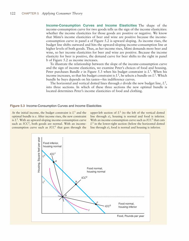
To illustrate the relationship between the slope of the income-consumption curveand the sign of income elasticities, we examine Peter’s choices of food and housing.Peter purchases Bundle e in Figure 5.3 when his budget constraint is When hisincome increases, so that his budget constraint is L2, he selects a bundle on Whichbundle he buys depends on his tastes—his indifference curves.
The horizontal and vertical dotted lines through e divide the new budget line, into three sections. In which of these three sections the new optimal bundle islocated determines Peter’s income elasticities of food and clothing.
L2,
L2.L1.
Hou
sing
,Squ
are
feet
per
yea
r
Food, Pounds per year
Food normal,housing normal
Food inferior,housing normal
Food normal,housing inferior
b
c
e
a
L1
L2
I
ICC2
ICC1
ICC3
Figure 5.3 Income-Consumption Curves and Income Elasticities
At the initial income, the budget constraint is and theoptimal bundle is e. After income rises, the new constraintis With an upward-sloping income-consumption curvesuch as both goods are normal. With an income-consumption curve such as that goes through the
upper-left section of (to the left of the vertical dottedline through e), housing is normal and food is inferior.With an income-consumption curve such as that cuts
in the lower-right section (below the horizontal dottedline through e), food is normal and housing is inferior.L2
ICC3
L2
ICC1ICC2,
L2.
L1

1235.2 How Changes in Income Shift Demand Curves
Suppose that Peter’s indifference curve is tangent to at a point in the upper-leftsection of (to the left of the vertical dotted line that goes through e) such as a. IfPeter’s income-consumption curve is which goes from e through a, he buysmore housing and less food as his income rises. (We draw the possible ICC curvesas straight lines for simplicity. In general, they may curve.) Housing is a normalgood, and food is an inferior good.
If instead the new optimal bundle is located in the middle section of (abovethe horizontal dotted line and to the right of the vertical dotted line), such as at b,his income-consumption curve through e and b is upward sloping. He buysmore of both goods as his income rises, so both food and housing are normal goods.
Third, suppose that his new optimal bundle is in the bottom-right segment of (below the horizontal dotted line). If his new optimal bundle is c, his income-consumption curve slopes downward from e through c. As his income rises,Peter consumes more food and less housing, so food is a normal good and housingis an inferior good.
Some Goods Must Be Normal It is impossible for all goods to be inferior. Weillustrate this point using Figure 5.3. At his original income, Peter faced budget con-straint and bought the combination of food and housing e. When his income goesup, his budget constraint shifts outward to Depending on his tastes (the shapeof his indifference curves), he may buy more housing and less food, such as Bundlea; more of both, such as b; or more food and less housing, such as c. Therefore,either both goods are normal or one good is normal and the other is inferior.
If both goods were inferior, Peter would buy less of both goods as his incomerises—which makes no sense. Were he to buy less of both, he would be buying a bun-dle that lies inside his original budget constraint Even at his original, relativelylow income, he could have purchased that bundle but chose not to, buying e instead.By the more-is-better assumption of Chapter 4, there is a bundle on the budget con-straint that gives Peter more utility than any given bundle inside the constraint.
Even if an individual does not buy more of the usual goods and services, that per-son may put the extra money into savings. Empirical studies find that savings is anormal good.
Income Elasticities May Vary with Income A good may be normal at someincome levels and inferior at others. When Gail was poor and her income increasedslightly, she ate meat more frequently, and her meat of choice was hamburger. Thus,when her income was low, hamburger was a normal good. As her income increasedfurther, however, she switched from hamburgers to steak. Thus, at higher incomes,hamburger is an inferior good.
We show Gail’s choice between hamburger (horizontal axis) and all other goods(vertical axis) in panel a of Figure 5.4. As Gail’s income increases, her budget lineshifts outward, from to and she buys more hamburger: Bundle lies to theright of As her income increases further, shifting her budget line outward to Gail reduces her consumption of hamburger: Bundle lies to the left of
Gail’s Engel curve in panel b captures the same relationship. At low incomes, herEngel curve is upward sloping, indicating that she buys more hamburger as herincome rises. At higher incomes, her Engel curve is backward bending.
As their incomes rise, many consumers switch between lower-quality (ham-burger) and higher-quality (steak) versions of the same good. This switching behav-ior explains the pattern of income elasticities across different-quality cars. Forexample, the income elasticity of demand for a Jetta is 2.1, an Accord is 2.2, a BMW700 Series is 4.4, and a Jaguar X-Type is 4.5 (see MyEconLab, Chapter 5, “IncomeElasticities of Demand for Cars”).
e2.e3
L3,e1.e2L2,L1
L1.
L2.L1
ICC3
L2
ICC2
L2
ICC1,L2
L2
See Question 6 andProblem 36.

124 CHAPTER 5 Applying Consumer Theory
5.3 Effects of a Price ChangeHolding tastes, other prices, and income constant, an increase in a price of a goodhas two effects on an individual’s demand. One is the substitution effect: the changein the quantity of a good that a consumer demands when the good’s price rises,holding other prices and the consumer’s utility constant. If utility is held constant,as the price of the good increases, consumers substitute other, now relatively cheapergoods, for that one.
The other effect is the income effect: the change in the quantity of a good a con-sumer demands because of a change in income, holding prices constant. An increasein price reduces a consumer’s buying power, effectively reducing the consumer’sincome or opportunity set and causing the consumer to buy less of at least somegoods. A doubling of the price of all the goods the consumer buys is equivalent toa drop in income to half its original level. Even a rise in the price of only one goodreduces a consumer’s ability to buy the same amount of all goods as previously. Forexample, if the price of food increases in China, the effective purchasing power of aChinese consumer falls substantially because one-third of Chinese consumers’income is spent on food (Statistical Yearbook of China, 2006).
Y2
Y1
Y1
Y2
Y3
Y3
L1
Y, I
ncom
e
L2
L3
e2
e3
e1
E2
E3
E1
I 1
I 2
I 3
Hamburger per year
Income-consumption curve
Hamburger per year
All
othe
r go
ods
per
year
(a) Indifference Curves and Budget Constraints
(b) Engel Curve
Engel curve
Figure 5.4 A Good That Is Both Inferior and Normal
When she was poor and her income increased, Gail boughtmore hamburger, so that hamburger was a normal good.However, as her income rose more and she became wealth-ier, she bought less hamburger (it was an inferior good)and more steak. (a) The forward slope of the income-consumption curve from to and the backward bendfrom to show this pattern. (b) The forward slope ofthe Engel curve at low incomes, to and the back-ward bend at higher incomes, to also show this pattern.
E3,E2
E2,E1
e3e2
e2e1
substitution effectthe change in the quantityof a good that a consumerdemands when the good’sprice changes, holdingother prices and the con-sumer’s utility constant
income effectthe change in the quantityof a good a consumerdemands because of achange in income, holdingprices constant
1255.3 Effects of a Price Change
When a price goes up, the total change in the quantity purchased is the sum of the substitution and income effects.6 When estimating the effects of a price changeon the quantity an individual demands, economists decompose this combined effectinto the two separate components. By doing so, they gain extra information that theycan use to answer questions about whether inflation measures are accurate, whetheran increase in tax rates will raise tax revenue, and what the effects are of governmentpolicies that compensate some consumers. For example, President Jimmy Carter,when advocating a tax on gasoline, and President Bill Clinton, when calling for anenergy tax, proposed providing an income compensation for poor consumers to off-set the harms of the taxes. We can use knowledge of the substitution and incomeeffects from a price change of energy to evaluate the effect of these policies.
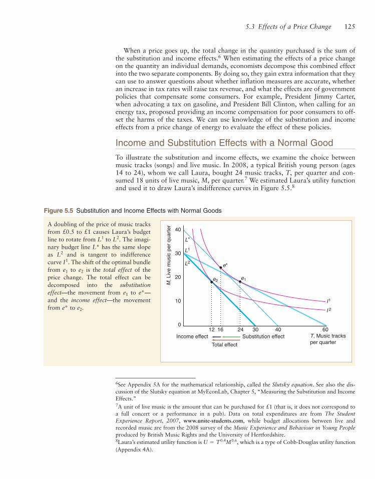
Income and Substitution Effects with a Normal GoodTo illustrate the substitution and income effects, we examine the choice betweenmusic tracks (songs) and live music. In 2008, a typical British young person (ages14 to 24), whom we call Laura, bought 24 music tracks, T, per quarter and con-sumed 18 units of live music, M, per quarter.7 We estimated Laura’s utility functionand used it to draw Laura’s indifference curves in Figure 5.5.8
6See Appendix 5A for the mathematical relationship, called the Slutsky equation. See also the dis-cussion of the Slutsky equation at MyEconLab, Chapter 5, “Measuring the Substitution and IncomeEffects.”7A unit of live music is the amount that can be purchased for £1 (that is, it does not correspond toa full concert or a performance in a pub). Data on total expenditures are from The StudentExperience Report, 2007, www.unite-students.com, while budget allocations between live andrecorded music are from the 2008 survey of the Music Experience and Behaviour in Young Peopleproduced by British Music Rights and the University of Hertfordshire.8Laura’s estimated utility function is which is a type of Cobb-Douglas utility function(Appendix 4A).
U = T0.4M0.6,
T, Music tracks per quarter
M, L
ive m
usic
per q
uarte
r
12 16 24 30 40 60
e2 e1
L2
L1
L*
e*
I 2I1
Income effectTotal effect
Substitution effect
40
30
20
10
0
Figure 5.5 Substitution and Income Effects with Normal Goods
A doubling of the price of music tracksfrom £0.5 to £1 causes Laura’s budgetline to rotate from to The imagi-nary budget line L* has the same slopeas and is tangent to indifferencecurve The shift of the optimal bundlefrom to is the total effect of theprice change. The total effect can bedecomposed into the substitutioneffect—the movement from to e*—and the income effect—the movementfrom e* to e2.
e1
e2e1
I1.L2
L2.L1

126 CHAPTER 5 Applying Consumer Theory
Because Laura’s entertainment budget for the quarter is Y = £30, the price of amusic track from Amazon.com or its major competitors is £0.5, and the price for aunit of live music is £1 (where we pick the unit appropriately), her original budgetconstraint is in Figure 5.5. She can afford to buy 60 music tracks and no livemusic, 30 units of live music and no music tracks, or any combination between theseextremes.
Given her estimated utility function, Laura’s demand functions are music tracks and At the original prices and with an entertainmentbudget of Y = £30 per quarter, Laura chooses Bundle music tracks and of live music per quarter, where herindifference curve is tangent to her budget constraint
Now suppose that the price of a music track doubles to £1, causing Laura’s bud-get constraint to rotate inward from to in Figure 5.5. The new budget con-straint, is twice as steep, as is
because music tracks are now twice as expensive. Laura’s oppor-tunity set is smaller, so she can choose between fewer music track–live music bun-dles than she could at the lower music track price. The area between the two budgetconstraints reflects the decrease in her opportunity set owing to the increase in theprice of music tracks. At this higher price for music tracks, Laura’s new optimalbundle is (where she buys music tracks), which occurswhere her indifference curve is tangent to
The movement from to is the total change in her consumption owing to therise in the price of music tracks. In particular, the total effect on Laura’s consump-tion of music tracks from the increase in the price of tracks is that she now buys
fewer tracks per quarter. In the figure, the red arrow pointing to theleft and labeled “Total effect” shows this decrease. We can break the total effect intoa substitution effect and an income effect.
As the price of music tracks increases, Laura’s opportunity set shrinks eventhough her income is unchanged. If, as a thought experiment, we compensate herfor this loss by giving her extra income, we can determine her substitution effect.The substitution effect is the change in the quantity demanded from a compensatedchange in the price of music tracks, which occurs when we increase Laura’s incomeby enough to offset the rise in the price of music tracks so that her utility stays con-stant. To determine the substitution effect, we draw an imaginary budget constraint,L*, that is parallel to and tangent to Laura’s original indifference curve, Thisimaginary budget constraint, L*, has the same slope, as because bothcurves are based on the new, higher price of music tracks. For L* to be tangent to
we need to increase Laura’s budget from £30 to £40 to offset the harm from thehigher price of music tracks. If Laura’s budget constraint were L*, she would chooseBundle e*, where she buys tracks.
Thus, if the price of tracks rises relative to that of live music and we hold Laura’sutility constant by raising her income, Laura’s optimal bundle shifts from to e*,which is the substitution effect. She buys fewer tracks per quarter, asthe arrow pointing to the left labeled “Substitution effect” shows.
Laura also faces an income effect because the increase in the price of tracksshrinks her opportunity set, so she must buy a bundle on a lower indifference curve.As a thought experiment, we can ask how much we would have to lower Laura’sincome while holding prices constant for her to choose a bundle on this new, lowerindifference curve. The income effect is the change in the quantity of a good a con-sumer demands because of a change in income, holding prices constant. The paral-lel shift of the budget constraint from L* to captures this effective decrease inincome. The movement from e* to is the income effect, as the arrow pointing toe2
L2
8(= 24 - 16)e1
T = 0.4 * 40/1 = 16
I1,
L2,!1,I1.L2
12(= 24 - 12)
e2e1
L2.I2T = 0.4 * 30/1 = 12e2
!0.5/1 = !0.5,!pT /pM =L1,!pT /pM = !1/1 = !1,L2,
L2L1
L1.I1M = 0.6 * 30/1 = 18 units
e1, T = 0.4 * 30/0.5 = 24M = 0.6Y/pM.
T = 0.4Y/pT
L1

1275.3 Effects of a Price Change
the left labeled “Income effect” shows. As her budget decreases from £40 to £30,Laura consumes fewer tracks per year.
The total effect from the price change is the sum of the substitution and incomeeffects, as the arrows show. Laura’s total effect in music tracks per year from a risein the price of music tracks is
Because indifference curves are convex to the origin, the substitution effect isunambiguous: Less of a good is consumed when its price rises. A consumer alwayssubstitutes a less expensive good for a more expensive one, holding utility constant.The substitution effect causes a movement along an indifference curve.
The income effect causes a shift to another indifference curve due to a change inthe consumer’s opportunity set. The direction of the income effect depends on theincome elasticity. Because a music track is a normal good for Laura, her incomeeffect is negative. Thus, both Laura’s substitution effect and her income effect go inthe same direction, so the total effect of the price rise must be negative.
Income and Substitution Effects with an Inferior GoodIf a good is inferior, the income effect goes in the opposite direction from the sub-stitution effect. For most inferior goods, the income effect is smaller than the sub-stitution effect. As a result, the total effect moves in the same direction as thesubstitution effect, but the total effect is smaller. However, the income effect canmore than offset the substitution effect in extreme cases. We now examine such acase.
Dennis chooses between spending his money on Chicago Bulls basketball gamesand on movies, as Figure 5.6 shows. When the price of movies falls, Dennis’ budgetline shifts from to The total effect of the price fall is the movement from to We can break this total movement into an income effect and a substitutioneffect.
Dennis’ income effect, the movement to the left from Bundle e* to Bundle isnegative, as the arrow pointing left labeled “Income effect” shows. The incomeeffect is negative because Dennis regards movies as an inferior good.
Dennis’ substitution effect for movies is positive because movies are now lessexpensive than they were before the price change. The substitution effect is themovement to the right from to e*.
The total effect of a price change, then, depends on which effect is larger. BecauseDennis’ negative income effect for movies more than offsets his positive substitutioneffect, the total effect of a drop in the price of movies is negative.9
A good is called a Giffen good if a decrease in its price causes the quantitydemanded to fall.10 Thus, going to the movies is a Giffen good for Dennis. The pricedecrease has an effect that is similar to an income increase: His opportunity setincreases as the price of movies drops. Dennis spends the money he saves on movies
e1
e2,
e2.e1L2.L1
Total effect!12
==
substitution effect!8
++
income effect(!4).
4(= 16 - 12)
See Question 7 andProblems 37 and 38.
9Economists mathematically decompose the total effect of a price change into substitution andincome effects to answer various business and policy questions: see “Measuring the Substitution andIncome Effects” and “International Comparison of Substitution and Income Effects” inMyEconLab, Chapter 5.10Robert Giffen, a nineteenth-century British economist, argued that poor people in Irelandincreased their consumption of potatoes when the price rose because of a blight. However, morerecent studies of the Irish potato famine dispute this observation.
Giffen gooda commodity for which adecrease in its pricecauses the quantitydemanded to fall

Next to its plant, a manufacturer of dinner plates has an outlet store that sellsplates of both first quality (perfect plates) and second quality (plates with slightblemishes). The outlet store sells a relatively large share of seconds. At its regu-lar stores elsewhere, the firm sells many more first-quality plates than second-quality plates. Why? (Assume that consumers’ tastes with respect to plates are thesame everywhere and that there is a cost, s, of shipping each plate from the fac-tory to the firm’s other stores.)
Answer
1. Determine how the relative prices of plates differ between the two types ofstores. The slope of the budget line consumers face at the factory outlet storeis where is the price of first-quality plates and is the price of thep2p1!p1/p2,
128 CHAPTER 5 Applying Consumer Theory
to buy more basketball tickets. Indeed, he decides to increase his purchase of bas-ketball tickets even further by reducing his purchase of movie tickets.
The demand curve for a Giffen good has an upward slope! Dennis’ demand curvefor movies is upward sloping because he goes to more movies at the higher price, than at the lower price,
The Law of Demand (Chapter 2), however, says that demand curves slope down-ward. You’re no doubt wondering how I’m going to worm my way out of thisapparent contradiction. The answer is that I claimed that the Law of Demand wasan empirical regularity, not a theoretical necessity. Although it’s theoretically possi-ble for a demand curve to slope upward, other than rice consumption in Hunan,China (Jensen and Miller, 2008), economists have found few, if any, real-worldexamples of Giffen goods.11
e2.e1,
See Question 8.
SOLVED PROBLEM 5.4
Bas
ketb
all t
icke
ts p
er y
ear
Movie tickets per year
L1
L*
Total effectIncome effectSubstitution effect
L2
e1
e2
e*
I1
I2
Figure 5.6 Giffen Good
Because a movie ticket is an infe-rior good for Dennis, the incomeeffect, the movement from to
resulting from a drop in theprice of movies is negative. Thisnegative income effect more thanoffsets the positive substitutioneffect, the movement from to
so the total effect, the move-ment from to is negative.Thus, a movie ticket is a Giffengood because as its price drops,Dennis consumes less of it.
e2,e1
e*,e1
e2,e*
11Battalio, Kagel, and Kogut (1991), however, showed in an experiment that quinine water is aGiffen good for lab rats!

According to the economic theory discussed in Solved Problem 5.4, we expectthat the relatively larger share of higher-quality goods will be shipped, thegreater the per-unit shipping fee. Is this theory true, and is the effect large? Toanswer these questions, Hummels and Skiba (2004) examined shipments
between 6,000 country pairs for morethan 5,000 goods. They found that dou-bling per-unit shipping costs results in a70% to 143% increase in the average price(excluding the cost of shipping) as a largershare of top-quality products are shipped.
The greater the distance between thetrading countries, the higher the cost ofshipping. Hummels and Skiba speculatethat the relatively high quality of Japanesegoods is due to that country’s relativelygreat distance to major importers.
1295.4 Cost-of-Living Adjustments
5.4 Cost-of-Living AdjustmentsIn spite of the cost of living, it’s still popular. —Kathleen Norris
By knowing both the substitution and income effects, we can answer questions thatwe could not if we knew only the total effect. For example, if firms have an estimateof the income effect, they can predict the impact of a negative income tax (a gift ofmoney from the government) on the consumption of their products. Similarly, if weknow the size of both effects, we can determine how accurately the governmentmeasures inflation.
See Questions 9 and 10.
APPLICATION
Shipping the Good Stuff Away
seconds. It costs the same to ship, s, a first-quality plate as a second becausethey weigh the same and have to be handled in the same way. At all otherstores, the firm adds the cost of shipping to the price it charges at its factoryoutlet store, so the price of a first-quality plate is and the price of a sec-ond is As a result, the slope of the budget line consumers face at theother retail stores is The seconds are relatively less expen-sive at the factory outlet than at other stores. For example, if
and the slope of the budget line is atthe outlet store and elsewhere. Thus, the first-quality plate costs twiceas much as a second at the outlet store but only 1.5 times as much elsewhere.
2. Use the relative price difference to explain why relatively more seconds arebought at the factory outlet. Holding a consumer’s income and tastes fixed, ifthe price of seconds rises relative to that of firsts (as we go from the factoryoutlet to other retail shops), most consumers will buy relatively more firsts.The substitution effect is unambiguous: Were they compensated so that theirutilities were held constant, consumers would unambiguously substitute firstsfor seconds. It is possible that the income effect could go in the other direc-tion; however, as most consumers spend relatively little of their total budgeton plates, the income effect is presumably small relative to the substitutioneffect. Thus, we expect relatively fewer seconds to be bought at the retailstores than at the factory outlet.
!3/2!2s = $1 per plate,p1 = $2, p2 = $1,
!(p1 + s)/(p2 + s).p2 + s.
p1 + s
130 CHAPTER 5 Applying Consumer Theory
Many long-term contracts and government programs include cost-of-livingadjustments (COLAs), which raise prices or incomes in proportion to an index ofinflation. Not only business contracts but also rental contracts, alimony payments,salaries, pensions, and Social Security payments are frequently adjusted in this man-ner over time. We will use consumer theory to show that a cost-of-living measurethat governments commonly use overestimates how the true cost of living changesover time. Because of this overestimate, you overpay your landlord if the rent onyour apartment rises with this measure.
Inflation IndexesThe prices of most goods rise over time. We call the increase in the overall price levelinflation.
Real Versus Nominal Prices The actual price of a good is called the nominalprice. The price adjusted for inflation is the real price.
Because the overall level of prices rises over time, nominal prices usually increasemore rapidly than real prices. For example, the nominal price of a McDonald’s ham-burger rose from 15¢ in 1955 to 89¢ in 2010, nearly a six-fold increase. However,the real price of a burger fell because the prices of other goods rose more rapidlythan that of a burger.
How do we adjust for inflation to calculate the real price? Governments measurethe cost of a standard bundle of goods for use in comparing prices over time. Thismeasure, as mentioned earlier in this chapter, is called the Consumer Price Index(CPI). Each month, the government reports how much it costs to buy the bundle ofgoods that an average consumer purchased in a base year (with the base year chang-ing every few years).
By comparing the cost of buying this bundle over time, we can determine howmuch the overall price level has increased. In the United States, the CPI was 26.8 in1955 and 218.0 in July 2010.12 The cost of buying the bundle of goods increased
from 1955 to 2010.We can use the CPI to calculate the real price of a hamburger over time. In terms
of 2010 dollars, the real price of a hamburger in 1955 was
If you could have purchased the hamburger in 1955 with 2010 dollars—which areworth less than 1955 dollars—the hamburger would have cost $1.22. The real pricein 2010 dollars (and the nominal price) of a hamburger in 2010 was only 89¢. Thus,the real price of a hamburger fell by over a quarter. If we compared the real pricesin both years using 1955 dollars, we would reach the same conclusion that the realprice of hamburgers fell by about a quarter.
Calculating Inflation Indexes The government collects data on the quantities andprices of 364 individual goods and services, such as housing, dental services, watchand jewelry repairs, college tuition fees, taxi fares, women’s hairpieces and wigs,hearing aids, slipcovers and decorative pillows, bananas, pork sausage, and funeralexpenses. These prices rise at different rates. If the government merely reported all
CPI for 2010CPI for 1955
* price of a burger = 218.026.8
* 15. L 1.22.
788%(L 218.0/26.8)
12The number 218.0 is not an actual dollar amount. Rather, it is the actual dollar cost of buying thebundle divided by a constant that was chosen so that the average expenditure in the period1982–1984 was 100.
1315.4 Cost-of-Living Adjustments
these price increases separately, most of us would find this information overwhelm-ing. It is much more convenient to use a single summary statistic, the CPI, whichtells us how prices rose on average.
We can use an example with only two goods, clothing and food, to show how theCPI is calculated. In the first year, consumers buy units of clothing and unitsof food at prices and We use this bundle of goods, and as our base bun-dle for comparison. In the second year, consumers buy and units at prices and
The government knows from its survey of prices each year that the price of cloth-ing in the second year is times as large as the price the previous year and theprice of food is times as large. If the price of clothing was $1 in the first yearand $2 in the second year, the price of clothing in the second year is or100%, larger than in the first year.
One way we can average the price increases of each good is to weight themequally. But do we really want to do that? Do we want to give as much weight tothe price increase for skateboards as to the price increase for automobiles? An alter-native approach is to give a larger weight to the price change of a good as we spendmore of our income on that good, its budget share. The CPI takes this approach toweighting, using budget shares.13
The CPI for the first year is the amount of income it takes to buy the market bas-ket actually purchased that year:
(5.1)
The cost of buying the first year’s bundle in the second year is
(5.2)
To calculate the rate of inflation, we determine how much more income it wouldtake to buy the first year’s bundle in the second year, which is the ratio of Equation5.1 to Equation 5.2:
For example, from July 2009 to July 2010, the U.S. CPI rose by fromto Thus, it cost 1.2% more in 2010 than in 2009 to buy the
same bundle of goods.The ratio reflects how much prices rise on average. By multiplying and
dividing the first term in the numerator by and multiplying and dividing the sec-ond term by we find that this index is equivalent to
where and are the budget shares of clothing and food inthe first or base year. The CPI is a weighted average of the price increase for eachgood, and where the weights are each good’s budget share in the baseyear, and θF.θC
pF2/pF
1,pC2 /pC
1
θF = pF1F1/Y1θC = pC
1C1/Y1
Y2
Y1=
¢pC2
pC1 ≤pC
1 C1 + ¢pF2
pF1 ≤pF
1 F1
Y1= ¢pC
2
pC1 ≤θC + ¢pF
2
pF1 ≤θF,
pF1,
pC1
Y2/Y1
Y2 = 218.0.Y1 = 215.41.012 L Y2/Y1
Y2
Y1=
pC2 C1 + pF
2 F1
pC1 C1 + pF
1 F1.
Y2 = pC2 C1 + pF
2 F1.
Y1 = pC1 C1 + pF
1 F1.
21 = 2 times,
pF2/pF
1pC
2 /pC1
pF2.
pC2F2C2
F1,C1pF1.pC
1F1C1
13This discussion of the CPI is simplified in a number of ways. Sophisticated adjustments are madeto the CPI that are ignored here, including repeated updating of the base year (chaining). See Pollak(1989) and Diewert and Nakamura (1993).
See Question 11.

132 CHAPTER 5 Applying Consumer Theory
Effects of Inflation AdjustmentsA CPI adjustment of prices in a long-term contract overcompensates for inflation.We use an example involving an employment contract to illustrate the differencebetween using the CPI to adjust a long-term contract and using a true cost-of-livingadjustment, which holds utility constant.
CPI Adjustment Klaas signed a long-term contract when he was hired. Accordingto the COLA clause in his contract, his employer increases his salary each year bythe same percentage as that by which the CPI increases. If the CPI this year is 5%higher than the CPI last year, Klaas’ salary rises automatically by 5% over lastyear’s.
Klaas spends all his money on clothing and food. His budget constraint in thefirst year is which we rewrite as
The intercept of the budget constraint, on the vertical (clothing) axis in Figure5.7 is and the slope of the constraint is The tangency of his indiffer-ence curve and the budget constraint determine his optimal consumption bun-dle in the first year, where he purchases and
In the second year, his salary rises with the CPI to so his budget constraint,in that year is
The new constraint, has a flatter slope, than because the price ofclothing rose more than the price of food. The new constraint goes through the orig-inal optimal bundle, because, by increasing his salary using the CPI, the firmensures that Klaas can buy the same bundle of goods in the second year that hechose in the first year.
He can buy the same bundle, but does he? The answer is no. His optimal bundlein the second year is where indifference curve is tangent to his new budget con-straint The movement from to is the total effect from the changes in thereal prices of clothing and food. This adjustment to his income does not keep himon his original indifference curve,
Indeed, Klaas is better off in the second year than in the first. The CPI adjustmentovercompensates for the change in inflation in the sense that his utility increases.
Klaas is better off because the prices of clothing and food did not increase by thesame amount. Suppose that the price of clothing and food had both increased byexactly the same amount. After a CPI adjustment, Klaas’ budget constraint in thesecond year, would be exactly the same as in the first year, so he wouldchoose exactly the same bundle, in the second year as in the first year.
Because the price of food rose by less than the price of clothing, is not the sameas Food became cheaper relative to clothing, so by consuming more food andless clothing Klaas has higher utility in the second year.
Had clothing become relatively less expensive, Klaas would have raised his utility in the second year by consuming relatively more clothing. Thus, it doesn’tmatter which good becomes relatively less expensive over time—it’s only necessaryfor one of them to become a relative bargain for Klaas to benefit from the CPI compensation.
L1.L2
e1,L1,L2,
I1.
e2e1L2.I2e2,
e1,
L1!pF2 / pC
2 ,L2,
C =Y2
pC2 -
pF2
pC2 F.
L2,Y2,
F1.C1e1,L1I1
!pF1 /pC
1 .Y1/pC1 ,
L1,
C =Y1
pC1 -
pF1
pC1 F.
Y1 = pC1C + pF
1F,
See Questions 12–14.

1335.4 Cost-of-Living Adjustments
True Cost-of-Living Adjustment We now know that a CPI adjustment overcom-pensates for inflation. What we want is a true cost-of-living index: an inflationindex that holds utility constant over time.
How big an increase in Klaas’ salary would leave him exactly as well off in thesecond year as in the first? We can answer this question by applying the same tech-nique we use to identify the substitution and income effects. We draw an imaginarybudget line, in Figure 5.7, that is tangent to so that Klaas’ utility remains con-stant but has the same slope as The income, corresponding to that imagi-nary budget constraint, is the amount that leaves Klaas’ utility constant. Had Klaasreceived in the second year instead of he would have chosen Bundle instead of Because is on the same indifference curve, as Klaas’ utilitywould be the same in both years.
e1,I1,e*e2.e*Y2,Y*
Y*,L2.I1,L*
C2
C1
C, U
nits
of c
loth
ing
per
year
e2
e1
I1
L1
e*
L* L2
I2
F, Units of food per year
Y2 /p2Y1/p1
Y1/p1
Y* /p2
F2F1 Y2/p2
Y2 /p2
C
C
C
F F F*
Figure 5.7 The Consumer Price Index
In the first year, when Klaas has an income of his opti-mal bundle is where indifference curve is tangent tohis budget constraint, In the second year, the price ofclothing rises more than the price of food. Because hissalary increases in proportion to the CPI, his second-yearbudget constraint, goes through so he can buy thesame bundle as in the first year. His new optimal bundle,
however, is where is tangent to The CPI adjust-ment overcompensates him for the increase in prices:Klaas is better off in the second year because his utility isgreater on than on With a smaller true cost-of-living adjustment, Klaas’ budget constraint, is tan-gent to at e*.I1
L*,I1.I2
L2.I2e2,
e1,L2,
L1.I1e1,
Y1,
134 CHAPTER 5 Applying Consumer Theory
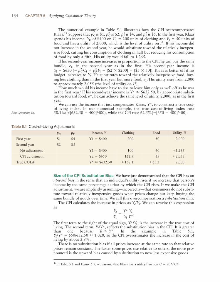
The numerical example in Table 5.1 illustrates how the CPI overcompensatesKlaas.14 Suppose that is $1, is $2, is $4, and is $5. In the first year, Klaasspends his income, of $400 on of clothing and offood and has a utility of 2,000, which is the level of utility on If his income didnot increase in the second year, he would substitute toward the relatively inexpen-sive food, cutting his consumption of clothing in half but reducing his consumptionof food by only a fifth. His utility would fall to 1,265.
If his second-year income increases in proportion to the CPI, he can buy the samebundle, in the second year as in the first. His second-year income is
Klaas is better off if hisbudget increases to He substitutes toward the relatively inexpensive food, buy-ing less clothing than in the first year but more food, His utility rises from 2,000to approximately 2,055 (the level of utility on ).
How much would his income have to rise to leave him only as well off as he wasin the first year? If his second-year income is by appropriate substi-tution toward food, he can achieve the same level of utility, 2,000, as in the firstyear.
We can use the income that just compensates Klaas, to construct a true cost-of-living index. In our numerical example, the true cost-of-living index rose
while the CPI rose 62.5%(= [650 - 400]/400).58.1%(L[632.50 - 400]/400),
Y*,
e*,Y* L $632.50,
I2e2.
Y2.Y2 = $650 (= pC
2 C1 + pF2 F1 = [$2 * $200] + [$5 * 50]).
e1,
I1.F1 = 50 unitsC1 = 200 unitsY1,
pF2pF
1pC2pC
1
14In Table 5.1 and Figure 5.7, we assume that Klaas has a utility function U = 202CF.
Table 5.1 Cost-of-Living Adjustments
pC pF Income, Y Clothing Food Utility, U
First year $1 $4 Y1 = $400 200 50 2,000
Second year $2 $5
No adjustment Y1 = $400 100 40 L1,265
CPI adjustment Y2 = $650 162.5 65 L2,055
True COLA Y* L +632.50 L158.1 L63.2 2,000
See Question 15.
Size of the CPI Substitution Bias We have just demonstrated that the CPI has anupward bias in the sense that an individual’s utility rises if we increase that person’sincome by the same percentage as that by which the CPI rises. If we make the CPIadjustment, we are implicitly assuming—incorrectly—that consumers do not substi-tute toward relatively inexpensive goods when prices change but keep buying thesame bundle of goods over time. We call this overcompensation a substitution bias.
The CPI calculates the increase in prices as We can rewrite this expressionas
The first term to the right of the equal sign, is the increase in the true cost ofliving. The second term, reflects the substitution bias in the CPI. It is greaterthan one because In the example in Table 5.1,
so the CPI overestimates the increase in the cost ofliving by about 2.8%.
There is no substitution bias if all prices increase at the same rate so that relativeprices remain constant. The faster some prices rise relative to others, the more pro-nounced is the upward bias caused by substitution to now less expensive goods.
Y2/Y* = 650/632.50 L 1.028,Y2 7 Y*.
Y2/Y*,Y*/Y1,
Y2
Y1= Y*
Y1
Y2
Y*.
Y2/Y1.
Several studies estimate that, due to the substitution bias, the CPI inflation rateis about half a percentage point too high per year. What can be done to correctthis bias? One approach is to estimate utility functions for individuals and usethose data to calculate a true cost-of-living index. However, given the widevariety of tastes across individuals, as well as various technical estimationproblems, this approach is not practical.
A second method is to use a Paasche index, which weights prices using thecurrent quantities of goods purchased. In contrast, the CPI (which is also calleda Laspeyres index) uses quantities from the earlier, base period. A Paascheindex is likely to overstate the degree of substitution and thus to understate thechange in the cost-of-living index. Hence, replacing the traditional Laspeyresindex with the Paasche would merely replace an overestimate with an under-estimate of the rate of inflation.
A third, compromise approach is to take an average of the Laspeyres andPaasche indexes because the true cost-of-living index lies between these twobiased indexes. The most widely touted average is the Fisher index, which is thegeometric mean of the Laspeyres and Paasche indexes (the square root of theirproduct). If we use the Fisher index, we are implicitly assuming that there is aunitary elasticity of substitution among goods so that the share of consumerexpenditures on each item remains constant as relative prices change (in contrastto the Laspeyres approach, where we assume that the quantities remain fixed).
Not everyone agrees that averaging the Laspeyres and Paasche indexeswould be an improvement. For example, if people do not substitute, the CPI(Laspeyres) index is correct and the Fisher index, based on the geometric aver-age, underestimates the rate of inflation.
Nonetheless, the Bureau of Labor Statistics (BLS), which calculates the CPI,has made several adjustments to its CPI methodology, including using averag-ing. Starting in 1999, the BLS replaced the Laspeyres index with a Fisherapproach to calculate almost all of its 200 basic indexes (such as “ice creamand related products”) within the CPI. It still uses the Laspeyres approach fora few of the categories in which it does not expect much substitution, such asutilities (electricity, gas, cable television, and telephones), medical care, andhousing, and it uses the Laspeyres method to combine the basic indexes toobtain the final CPI.
Now, the BLS updates the CPI weights (the market basket shares of con-sumption) every two years instead of only every decade or so, as the Bureauhad done before 2002. More frequent updating reduces the substitution bias ina Laspeyres index because market basket shares are frozen for a shorter periodof time. According to the BLS, had it used updated weights between 1989 and1997, the CPI would have increased by only 31.9% rather than the reported33.9%. Thus, the BLS believes that this change will reduce the rate of increasein the CPI by approximately 0.2 percentage points per year.
Overestimating the rate of inflation has important implications for U.S.society because Social Security, various retirement plans, welfare, and manyother programs include CPI-based cost-of-living adjustments. According to oneestimate, the bias in the CPI alone makes it the fourth-largest “federal pro-gram” after Social Security, health care, and defense. For example, the U.S.Postal Service (USPS) has a CPI-based COLA in its union contracts. In 2010, atypical employee earned about $51,000 a year. Consequently, the estimatedsubstitution bias of half a percent a year cost the USPS nearly $255 peremployee, or about $195 million, because the USPS had about 764,000employees at the time.
1355.4 Cost-of-Living Adjustments
See Question 16.
APPLICATION
Fixing the CPISubstitution Bias
136 CHAPTER 5 Applying Consumer Theory
5.5 Deriving Labor Supply CurvesThe human race is faced with a cruel choice: work or daytime television.
Throughout this chapter, we’ve used consumer theory to examine consumers’demand behavior. Perhaps surprisingly, we can use the consumer theory model toderive the supply curve of labor. We are going to do that by deriving a demand curvefor time spent not working and then using that demand curve to determine the sup-ply curve of hours spent working.
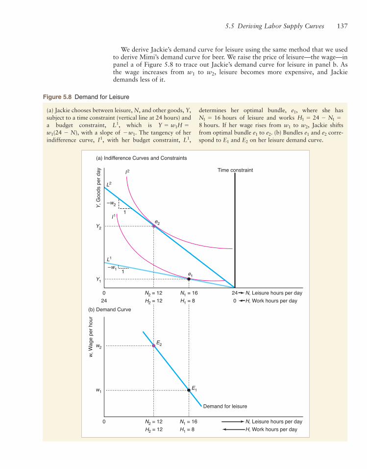
Labor-Leisure ChoicePeople choose between working to earn money to buy goods and services and con-suming leisure: all time spent not working. In addition to sleeping, eating, and play-ing, leisure includes time spent cooking meals and fixing things around the house.The number of hours worked per day, H, equals 24 minus the hours of leisure ornonwork, N, in a day:
Using consumer theory, we can determine the demand curve for leisure once weknow the price of leisure. What does it cost you to watch TV or go to school or doanything for an hour other than work? It costs you the wage, w, you could haveearned from an hour’s work: The price of leisure is forgone earnings. The higheryour wage, the more an hour of leisure costs you. For this reason, taking an after-noon off costs a lawyer who earns $250 an hour much more than it costs someonewho earns the minimum wage.
We use an example to show how the number of hours of leisure and workdepends on the wage, unearned income (such as inheritances and gifts from par-ents), and tastes. Jackie spends her total income, Y, on various goods. For simplic-ity, we assume that the price of these goods is $1 per unit, so she buys Y goods. Herutility, U, depends on how many goods and how much leisure she consumes:
Initially, we assume that Jackie can choose to work as many or as few hours asshe wants for an hourly wage of w. Jackie’s earned income equals her wage timesthe number of hours she works, wH. Her total income, Y, is her earned income plusher unearned income,
Panel a of Figure 5.8 shows Jackie’s choice between leisure and goods. The ver-tical axis shows how many goods, Y, Jackie buys. The horizontal axis shows bothhours of leisure, N, which are measured from left to right, and hours of work, H,which are measured from right to left. Jackie maximizes her utility given the twoconstraints she faces. First, she faces a time constraint, which is a vertical line at 24hours of leisure. There are only 24 hours in a day; all the money in the world won’tbuy her more hours in a day. Second, Jackie faces a budget constraint. BecauseJackie has no unearned income, her initial budget constraint, is
The slope of her budget constraint is because eachextra hour of leisure she consumes costs her goods.
Jackie picks her optimal hours of leisure, so that she is on the highestindifference curve, that touches her budget constraint. She works
per day and earns an income of Y1 = w1H1 = 8w1.H1 = 24 - N1 = 8 hoursI1,
N1 = 16,w1
!w1,Y = w1H = w1(24 - N).L1,
Y = wH + Y*.
Y*:
U = U(Y, N).
H = 24 - N.
1375.5 Deriving Labor Supply Curves
Y, G
oods
per d
ay Time constraint
H2 = 12 H1 = 824 0N2 = 12 N1 = 160 24
H, Work hours per dayN, Leisure hours per day
H2 = 12 H1 = 8N2 = 12 N1 = 160
H, Work hours per dayN, Leisure hours per day
Demand for leisure
I 2
I1 1–w2
L1
L2
(a) Indifference Curves and Constraints
w, W
age p
er ho
ur
(b) Demand Curve
–w1 1
e2Y2
Y1
w1
w2
e1
E2
E1
Figure 5.8 Demand for Leisure
(a) Jackie chooses between leisure, N, and other goods, Y,subject to a time constraint (vertical line at 24 hours) anda budget constraint, which is
with a slope of The tangency of herindifference curve, with her budget constraint,
determines her optimal bundle, where she hasof leisure and works
If her wage rises from to Jackie shiftsfrom optimal bundle to (b) Bundles and corre-spond to and on her leisure demand curve.E2E1
e2e1e2.e1
w2,w18 hours.24 - N1 =H1 =N1 = 16 hours
e1,
L1,I1,!w1.w1(24 - N),
Y = w1H =L1,
We derive Jackie’s demand curve for leisure using the same method that we usedto derive Mimi’s demand curve for beer. We raise the price of leisure—the wage—inpanel a of Figure 5.8 to trace out Jackie’s demand curve for leisure in panel b. Asthe wage increases from to leisure becomes more expensive, and Jackiedemands less of it.
w2,w1
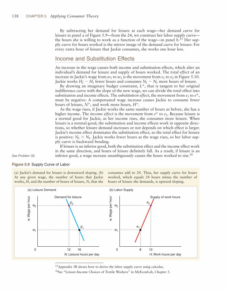
138 CHAPTER 5 Applying Consumer Theory
15Appendix 5B shows how to derive the labor supply curve using calculus.
By subtracting her demand for leisure at each wage—her demand curve forleisure in panel a of Figure 5.9—from the 24, we construct her labor supply curve—the hours she is willing to work as a function of the wage—in panel b.15 Her sup-ply curve for hours worked is the mirror image of the demand curve for leisure: Forevery extra hour of leisure that Jackie consumes, she works one hour less.
Income and Substitution EffectsAn increase in the wage causes both income and substitution effects, which alter anindividual’s demand for leisure and supply of hours worked. The total effect of anincrease in Jackie’s wage from to is the movement from to in Figure 5.10.Jackie works fewer hours and consumes more hours of leisure.
By drawing an imaginary budget constraint, that is tangent to her originalindifference curve with the slope of the new wage, we can divide the total effect intosubstitution and income effects. The substitution effect, the movement from to must be negative: A compensated wage increase causes Jackie to consume fewerhours of leisure, and work more hours,
As the wage rises, if Jackie works the same number of hours as before, she has ahigher income. The income effect is the movement from to Because leisure isa normal good for Jackie, as her income rises, she consumes more leisure. Whenleisure is a normal good, the substitution and income effects work in opposite direc-tions, so whether leisure demand increases or not depends on which effect is larger.Jackie’s income effect dominates the substitution effect, so the total effect for leisureis positive: Jackie works fewer hours as the wage rises, so her labor sup-ply curve is backward bending.
If leisure is an inferior good, both the substitution effect and the income effect workin the same direction, and hours of leisure definitely fall. As a result, if leisure is aninferior good, a wage increase unambiguously causes the hours worked to rise.16
N2 7 N1.
e2.e*
H*.N*,
e*,e1
L*,N2 - N1H2 - H1
e2e1w2w1
See Problem 39.
w, W
age
per
hour
(a) Leisure Demand
Demand for leisure
w1
w2
16120N, Leisure hours per day
E1
E2
w, W
age
per
hour
(b) Labor Supply
Supply of work hours
w1
w2
8 120H, Work hours per day
e2
e1
Figure 5.9 Supply Curve of Labor
(a) Jackie’s demand for leisure is downward sloping. (b)At any given wage, the number of hours that Jackieworks, H, and the number of hours of leisure, N, that she
consumes add to 24. Thus, her supply curve for hoursworked, which equals 24 hours minus the number ofhours of leisure she demands, is upward sloping.
16See “Leisure-Income Choices of Textile Workers” in MyEconLab, Chapter 5.
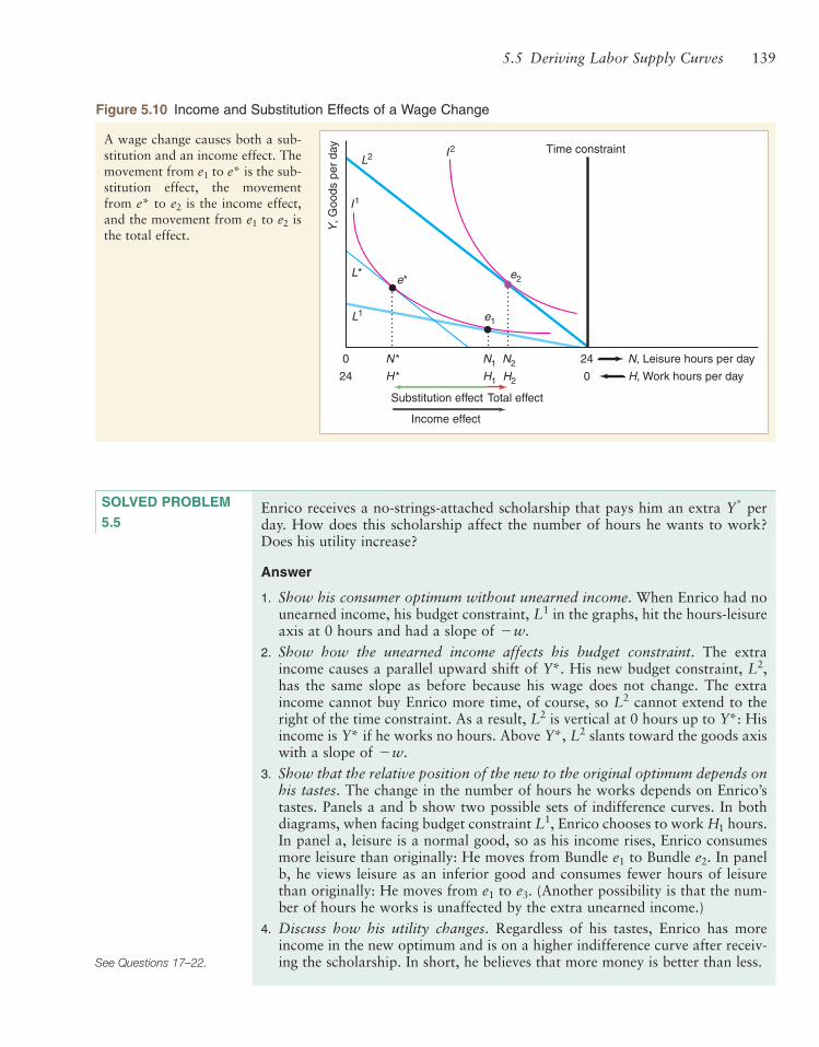
Enrico receives a no-strings-attached scholarship that pays him an extra perday. How does this scholarship affect the number of hours he wants to work?Does his utility increase?
Answer
1. Show his consumer optimum without unearned income. When Enrico had nounearned income, his budget constraint, in the graphs, hit the hours-leisureaxis at 0 hours and had a slope of
2. Show how the unearned income affects his budget constraint. The extraincome causes a parallel upward shift of His new budget constraint, has the same slope as before because his wage does not change. The extraincome cannot buy Enrico more time, of course, so cannot extend to theright of the time constraint. As a result, is vertical at 0 hours up to Hisincome is if he works no hours. Above slants toward the goods axiswith a slope of
3. Show that the relative position of the new to the original optimum depends onhis tastes. The change in the number of hours he works depends on Enrico’stastes. Panels a and b show two possible sets of indifference curves. In bothdiagrams, when facing budget constraint Enrico chooses to work hours.In panel a, leisure is a normal good, so as his income rises, Enrico consumesmore leisure than originally: He moves from Bundle to Bundle In panelb, he views leisure as an inferior good and consumes fewer hours of leisurethan originally: He moves from to (Another possibility is that the num-ber of hours he works is unaffected by the extra unearned income.)
4. Discuss how his utility changes. Regardless of his tastes, Enrico has moreincome in the new optimum and is on a higher indifference curve after receiv-ing the scholarship. In short, he believes that more money is better than less.
e3.e1
e2.e1
H1L1,
!w.Y*, L2Y*
Y*:L2L2
L2,Y*.
!w.L1
Y*
1395.5 Deriving Labor Supply Curves
Y, G
oods
per
day Time constraint
H2H* H124 0N2N* N10 24
Substitution effect
Income effect
Total effect
H, Work hours per dayN, Leisure hours per day
I2
I1
L2
L*
L1
e2
e1
e*
Figure 5.10 Income and Substitution Effects of a Wage Change
A wage change causes both a sub-stitution and an income effect. Themovement from to is the sub-stitution effect, the movementfrom to is the income effect,and the movement from to isthe total effect.
e2e1
e2e*
e*e1
SOLVED PROBLEM 5.5
See Questions 17–22.

140 CHAPTER 5 Applying Consumer Theory
Shape of the Labor Supply CurveWhether the labor supply curve slopes upward, bends backward, or has sectionswith both properties depends on the income elasticity of leisure. Suppose that aworker views leisure as an inferior good at low wages and a normal good at highwages. As the wage increases, the demand for leisure first falls and then rises, andthe hours supplied to the market first rise and then fall. (Alternatively, the labor sup-ply curve may slope upward and then backward even if leisure is normal at allwages: At low wages, the substitution effect—work more hours—dominates theincome effect—work fewer hours—while the opposite occurs at higher wages.)
The budget line rotates upward from to as the wage rises in panel a ofFigure 5.11. Because leisure is an inferior good at low incomes, in the new optimalbundle, this worker consumes less leisure and more goods than at the originalbundle,
At higher incomes, however, leisure is a normal good. At an even higher wage,the new optimum is on budget line where the quantity of leisure demandedis higher and the number of hours worked is lower. Thus, the corresponding supplycurve for labor slopes upward at low wages and bends backward at higher wages inpanel b.
Do labor supply curves slope upward or backward? Economic theory alone can-not answer this question: Both forward-sloping and backward-bending supply curvesare theoretically possible. Empirical research is necessary to resolve this question.
Most studies (Killingsworth, 1983; MaCurdy, Green, and Paarsch, 1990) findthat the labor supply curves for single and married British and American men arevirtually vertical because both the income and substitution effects are about zero.Studies find that married women’s labor supply curves are also virtually vertical:slightly backward bending in Canada and the United States and slightly forwardsloping in the United Kingdom and Germany. In contrast, studies of the labor sup-ply of single women find relatively large positive supply elasticities of 4.0 and evenhigher. Thus, only single women tend to work substantially more hours when theirwages rise.
L3,e3,
e1.e2,
L2L1
Y, G
oods
per
day
(a) Leisure Normal
Time constraint
H2 H3H124 0H, Work hours per day
L2
I2
I1
L1
Y*
e2
e1
Y, G
oods
per
day
(b) Leisure Inferior
Time constraint
H124 0H, Work hours per day
L2
I1
L1
Y*
e1I3
e3

Would you stop working if you won a lottery jackpot or inherited a large sum?Economists want to know how unearned income affects the amount of laborpeople are willing to supply because this question plays a crucial role in manygovernment debates on taxes and welfare. For example, some legislatorsoppose negative income tax and welfare programs because they claim that giv-ing money to poor people will stop them from working. Is that assertion true?
We could clearly answer this question if we could observe the behavior of alarge group of people, only some of whom were randomly selected to receivevarying but large amounts of unearned income each year for decades. Luckilyfor us, governments conduct such experiments by running lotteries.
Imbens et al. (2001) compared the winners of major prizes to others whoplayed the Massachusetts Megabucks lottery. Major prizes ranged from$22,000 to $9.7 million, with an average of $1.1 million, and were paid inyearly installments over two decades.
A typical player in this lottery earned $16,100. The average winner received$55,200 in prize money per year and chose to work slightly fewer hours so thathis or her labor earnings fell by $1,877 per year. That is, winners increasedtheir consumption and savings but did not substantially decrease how muchthey worked.
For every dollar of unearned income, winners reduced their work effort andhence their labor earnings by 11¢ on average. Men and women, big and verybig prize winners, and people of all education levels behaved the same way.However, the behavior of winners differed by age and by income groups.People ages 55 to 65 reduced their labor efforts by about a third more thanyounger people did, presumably because they decided to retire early. Moststriking, people with no earnings in the year before winning the lottery tendedto increase their labor earnings after winning.
1415.5 Deriving Labor Supply Curves
Y, G
oods
per
day
(a) Labor-Leisure Choice
Time constraint
H2 H3 H124 0H, Work hours per day
E1
E3
E2
L2
I2
I3
I1
L3
L1
e2
e1
e3
w, W
age
per
hour
(b) Supply Curve of Labor
Supply curve of labor
H2H3H1 240H, Work hours per day
Figure 5.11 Labor Supply Curve That Slopes Upward and Then Bends Backward
At low incomes, an increase in the wage causes theworker to work more: the movement from to inpanel a or from to in panel b. At higher incomes,
an increase in the wage causes the worker to work fewerhours: the movement from to or from to E3.E2e3e2
E2E1
e2e1
APPLICATION
Working After Winningthe Lottery
See Question 23.

142 CHAPTER 5 Applying Consumer Theory
Income Tax Rates and Labor SupplyThe wages of sin are death, but by the time taxes are taken out, it’s just sortof a tired feeling. —Paula Poundstone
Why do we care about the shape of labor supply curves? One reason is that we cantell from the shape of the labor supply curve whether an increase in the income taxrate—a percent of earnings—will cause a substantial reduction in the hours ofwork.17 Taxes on earnings are an unattractive way of collecting money for the gov-ernment if supply curves are upward sloping because the taxes cause people to workfewer hours, reducing the amount of goods society produces and raising less tax rev-enue than if the supply curve were vertical or backward bending. On the other hand,if supply curves are backward bending, a small increase in the tax rate increases taxrevenue and boosts total production (but reduces leisure).
Although unwilling to emulate Lady Godiva’s tax-fighting technique—allegedly,her husband, Leofric, the Earl of Mercia, agreed to eliminate taxes if she rode nakedthrough the Coventry marketplace—various U.S. presidents have advocated taxcuts. Presidents John F. Kennedy, Ronald Reagan, and George W. Bush argued thatcutting the marginal tax rate (the percentage of the last dollar earned that the gov-ernment takes in taxes) would stimulate people to work longer and produce more,both desirable effects. President Reagan claimed that tax receipts would increasedue to the additional work.
Because tax rates have changed substantially over time, we have a natural exper-iment to test this hypothesis. The Kennedy tax cuts lowered the top personalmarginal tax rate from 91% to 70%. Due to the Reagan tax cuts, the maximum ratefell to 50% from 1982 to 1986, 38.5% in 1987, and 28% in 1988–1990. The raterose to 31% in 1991–1992 and 39.6% from 1993 to 2000. The Bush administra-tion’s Tax Relief Act of 2001 tax cut reduced this rate to 38.6% for 2001–2003,37.6% for 2004–2005, and 35% for 2006 and thereafter.
Many other countries’ central governments have also lowered their top marginaltax rates in recent years. The top U.K. rate fell sharply during the Thatcher admin-istration from 83% to 60% in 1979 and to 40% in 1988, but it rose to 50% in2010. Japan’s top rate fell from 75% in 1983 to 60% in 1987, to 50% in 1988, andto 37% in 1999, but it rose to 40% in 2007. In 1988, Canada raised the marginaltax rates for the two lowest income groups and lowered them for those falling intothe top nine brackets.
Kuhn et al. (2008) examined the Dutch Postcode Lottery, in which prizes areawarded weekly to lottery participants living in randomly selected postalcodes. On average, the prizes are equal to about eight months of income.Household heads who received prizes did not change how many hours theyworked.
However, Highhouse et al. (2010) reported a decline in the “American workethic” based on surveys. In 1955, 80% of working U.S. males said that theywould continue to work even if they inherited enough to live comfortably. Thatshare dropped to 72% in the mid-1970s. Currently, given a large lottery win,only about 68% said they would continue to work.
17Although taxes are ancient, the income tax is a relatively recent invention. William Pitt theYounger introduced the British income tax (10% on annual incomes above £60) in 1798 to financethe war with Napoleon. The U.S. Congress followed suit in 1861, using the income taxes (3% onannual incomes over $800) to pay for the Civil War.
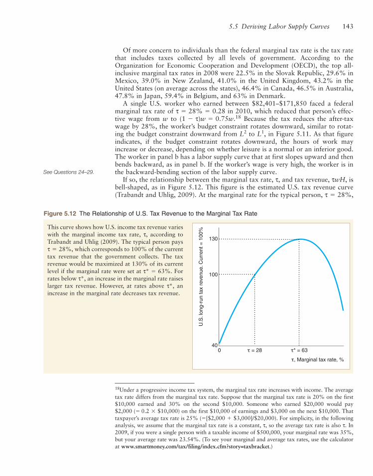
1435.5 Deriving Labor Supply Curves
See Questions 24–29.
Of more concern to individuals than the federal marginal tax rate is the tax ratethat includes taxes collected by all levels of government. According to theOrganization for Economic Cooperation and Development (OECD), the top all-inclusive marginal tax rates in 2008 were 22.5% in the Slovak Republic, 29.6% inMexico, 39.0% in New Zealand, 41.0% in the United Kingdom, 43.2% in theUnited States (on average across the states), 46.4% in Canada, 46.5% in Australia,47.8% in Japan, 59.4% in Belgium, and 63% in Denmark.
A single U.S. worker who earned between $82,401–$171,850 faced a federalmarginal tax rate of in 2010, which reduced that person’s effec-tive wage from w to 18 Because the tax reduces the after-taxwage by 28%, the worker’s budget constraint rotates downward, similar to rotat-ing the budget constraint downward from to in Figure 5.11. As that figureindicates, if the budget constraint rotates downward, the hours of work mayincrease or decrease, depending on whether leisure is a normal or an inferior good.The worker in panel b has a labor supply curve that at first slopes upward and thenbends backward, as in panel b. If the worker’s wage is very high, the worker is inthe backward-bending section of the labor supply curve.
If so, the relationship between the marginal tax rate, and tax revenue, isbell-shaped, as in Figure 5.12. This figure is the estimated U.S. tax revenue curve(Trabandt and Uhlig, 2009). At the marginal rate for the typical person, τ = 28%,
τwH,τ,
L1,L2
(1 - τ)w = 0.75w.τ = 28% = 0.28
18Under a progressive income tax system, the marginal tax rate increases with income. The averagetax rate differs from the marginal tax rate. Suppose that the marginal tax rate is 20% on the first$10,000 earned and 30% on the second $10,000. Someone who earned $20,000 would pay
on the first $10,000 of earnings and $3,000 on the next $10,000. Thattaxpayer’s average tax rate is For simplicity, in the followinganalysis, we assume that the marginal tax rate is a constant, so the average tax rate is also In2009, if you were a single person with a taxable income of $500,000, your marginal rate was 35%,but your average rate was 23.54%. (To see your marginal and average tax rates, use the calculatorat www.smartmoney.com/tax/filing/index.cfm?story=taxbracket.)
τ.τ,25% (= [$2,000 + $3,000]/$20,000).
$2,000 (= 0.2 * $10,000)
U.S
. lon
g-ru
n ta
x re
venu
e. C
urre
nt =
100
%
130
100
400 τ = 28 τ* = 63
τ, Marginal tax rate, %
Figure 5.12 The Relationship of U.S. Tax Revenue to the Marginal Tax Rate
This curve shows how U.S. income tax revenue varieswith the marginal income tax rate, according toTrabandt and Uhlig (2009). The typical person pays
which corresponds to 100% of the currenttax revenue that the government collects. The taxrevenue would be maximized at 130% of its currentlevel if the marginal rate were set at Forrates below an increase in the marginal rate raiseslarger tax revenue. However, at rates above anincrease in the marginal rate decreases tax revenue.
τ*,τ*,
τ* = 63%.
τ = 28%,
τ,

If a country’s marginal income tax rate is initially on the upward-sloping sec-tion to the left of the peak of the bell-shaped tax revenue curve below as inFigure 5.12, then raising increases tax revenue but causes people to workfewer hours. If the initial rate is on the “wrong side” of the revenue curve tothe right of then reducing will raise tax revenues and hours worked.
Trabandt and Uhlig (2009) calculated the potential revenue gains fromadjusting the tax rate to The following table summarizes their results forthe United States and 14 European Union countries, where EU-14 is the aver-age for the 14 EU countries and all numbers are percentages. The first columnis the typical marginal tax-rate percentage, the second column shows the ratethat maximizes tax collections, and the final column is the maximum pos-sible percentage increase in tax revenue that can be obtained in the long run,by raising or lowering to equal Denmark is (slightly) on the wrong sideτ*.τ
τ*;τ;
τ*.
ττ*,
ττ*
144 CHAPTER 5 Applying Consumer Theory
the government collects 100% of the amount of tax revenue it’s currently collecting.At a zero tax rate, a small increase in the tax rate must increase the tax revenuebecause no revenue was collected when the tax rate was zero. However, if the taxrate rises a little more, the tax revenue collected must rise even higher, for two rea-sons: First, the government collects a larger percentage of every dollar earnedbecause the tax rate is higher. Second, employees work more hours as the tax raterises because workers are in the backward-bending sections of their labor supplycurves.
As the marginal rate increases, tax revenue rises until the marginal rate reacheswhere the U.S. tax revenue would be 130% of its current level. If the
marginal tax rate increases more, workers are in the upward-sloping sections oftheir labor supply curves, so an increase in the tax rate reduces the number of hoursworked. When the tax rate rises high enough, the reduction in hours worked morethan offsets the gain from the higher rate, so the tax revenue falls.
It makes little sense for a government to operate at very high marginal tax ratesin the downward-sloping portion of this bell-shaped curve. The government couldget more output and more tax revenue by cutting the marginal tax rate.
τ* = 63%,
APPLICATION
Maximizing Income Tax Revenue
τ τ*Maximum Additional
Tax Revenue
United States 28 63 30EU-14 41 62 8Ireland 27 68 30United Kingdom 28 59 17Portugal 31 59 14Spain 36 62 13Germany 41 64 10Netherlands 44 67 9Greece 41 60 7France 46 63 5Italy 47 62 4Belgium 49 61 3Finland 49 62 3Austria 50 61 2Sweden 56 63 1Denmark 57 55 1
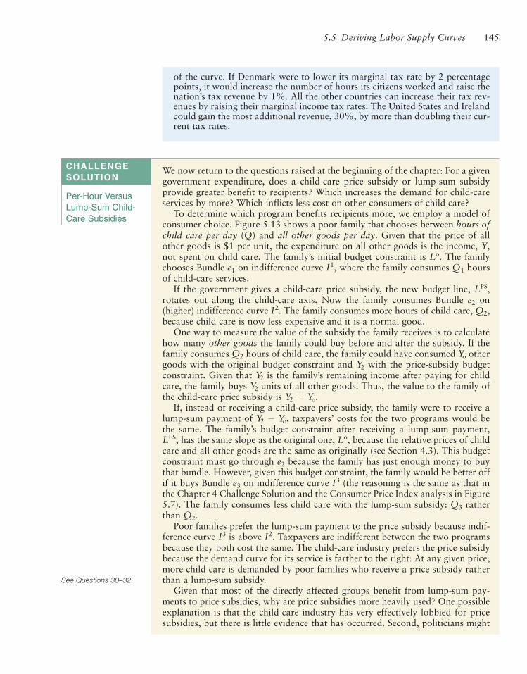
1455.5 Deriving Labor Supply Curves
See Questions 30–32.
of the curve. If Denmark were to lower its marginal tax rate by 2 percentagepoints, it would increase the number of hours its citizens worked and raise thenation’s tax revenue by 1%. All the other countries can increase their tax rev-enues by raising their marginal income tax rates. The United States and Irelandcould gain the most additional revenue, 30%, by more than doubling their cur-rent tax rates.
We now return to the questions raised at the beginning of the chapter: For a givengovernment expenditure, does a child-care price subsidy or lump-sum subsidyprovide greater benefit to recipients? Which increases the demand for child-careservices by more? Which inflicts less cost on other consumers of child care?
To determine which program benefits recipients more, we employ a model ofconsumer choice. Figure 5.13 shows a poor family that chooses between hours ofchild care per day (Q) and all other goods per day. Given that the price of allother goods is $1 per unit, the expenditure on all other goods is the income, Y,not spent on child care. The family’s initial budget constraint is The familychooses Bundle on indifference curve where the family consumes hoursof child-care services.
If the government gives a child-care price subsidy, the new budget line, rotates out along the child-care axis. Now the family consumes Bundle on(higher) indifference curve The family consumes more hours of child care, because child care is now less expensive and it is a normal good.
One way to measure the value of the subsidy the family receives is to calculatehow many other goods the family could buy before and after the subsidy. If thefamily consumes hours of child care, the family could have consumed othergoods with the original budget constraint and with the price-subsidy budgetconstraint. Given that is the family’s remaining income after paying for childcare, the family buys units of all other goods. Thus, the value to the family ofthe child-care price subsidy is
If, instead of receiving a child-care price subsidy, the family were to receive alump-sum payment of taxpayers’ costs for the two programs would bethe same. The family’s budget constraint after receiving a lump-sum payment,
has the same slope as the original one, because the relative prices of childcare and all other goods are the same as originally (see Section 4.3). This budgetconstraint must go through because the family has just enough money to buythat bundle. However, given this budget constraint, the family would be better offif it buys Bundle on indifference curve (the reasoning is the same as that inthe Chapter 4 Challenge Solution and the Consumer Price Index analysis in Figure5.7). The family consumes less child care with the lump-sum subsidy: ratherthan
Poor families prefer the lump-sum payment to the price subsidy because indif-ference curve is above Taxpayers are indifferent between the two programsbecause they both cost the same. The child-care industry prefers the price subsidybecause the demand curve for its service is farther to the right: At any given price,more child care is demanded by poor families who receive a price subsidy ratherthan a lump-sum subsidy.
Given that most of the directly affected groups benefit from lump-sum pay-ments to price subsidies, why are price subsidies more heavily used? One possibleexplanation is that the child-care industry has very effectively lobbied for pricesubsidies, but there is little evidence that has occurred. Second, politicians might
I2.I3
Q2.Q3
I3e3
e2
Lo,LLS,
Y2 - Yo,
Y2 - Yo.Y2
Y2
Y2
YoQ2
Q2,I2.e2
LPS,
Q1I1,e1
Lo.
CHALLENGESOLUTION
Per-Hour VersusLump-Sum Child-Care Subsidies
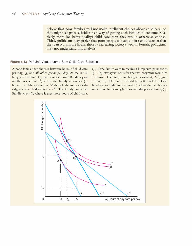
146 CHAPTER 5 Applying Consumer Theory
believe that poor families will not make intelligent choices about child care, sothey might see price subsidies as a way of getting such families to consume rela-tively more (or better-quality) child care than they would otherwise choose.Third, politicians may prefer that poor people consume more child care so thatthey can work more hours, thereby increasing society’s wealth. Fourth, politiciansmay not understand this analysis.
All o
ther g
oods
per d
ay
Q2Q3Q10 Q, Hours of day care per day
I2I3
I1
LPSLLSLo
e2e1
Y2
Yo
e3
Figure 5.13 Per-Unit Versus Lump-Sum Child Care Subsidies
A poor family that chooses between hours of child careper day, Q, and all other goods per day. At the initialbudget constraint, the family chooses Bundle onindifference curve where the family consumes hours of child-care services. With a child-care price sub-sidy, the new budget line is The family consumesBundle on where it uses more hours of child care,
If the family were to receive a lump-sum payment oftaxpayers’ costs for the two programs would be
the same. The lump-sum budget constraint, goesthrough The family would be better off if it buysBundle on indifference curve where the family con-sumes less child care, than with the price subsidy, Q2.Q3,
I3,e3
e2.LLS,
Y2 - Yo,Q2.
I2,e2
LPS.
Q1I1,e1Lo,
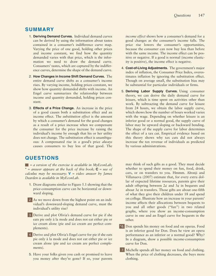
1. Deriving Demand Curves. Individual demand curvescan be derived by using the information about tastescontained in a consumer’s indifference curve map.Varying the price of one good, holding other pricesand income constant, we find how the quantitydemanded varies with that price, which is the infor-mation we need to draw the demand curve.Consumers’ tastes, which are captured by the indiffer-ence curves, determine the shape of the demand curve.
2. How Changes in Income Shift Demand Curves. Theentire demand curve shifts as a consumer’s incomerises. By varying income, holding prices constant, weshow how quantity demanded shifts with income. AnEngel curve summarizes the relationship betweenincome and quantity demanded, holding prices con-stant.
3. Effects of a Price Change. An increase in the priceof a good causes both a substitution effect and anincome effect. The substitution effect is the amountby which a consumer’s demand for the good changesas a result of a price increase when we compensatethe consumer for the price increase by raising theindividual’s income by enough that his or her utilitydoes not change. The substitution effect is unambigu-ous: A compensated rise in a good’s price alwayscauses consumers to buy less of that good. The
income effect shows how a consumer’s demand for agood changes as the consumer’s income falls. Theprice rise lowers the consumer’s opportunities,because the consumer can now buy less than beforewith the same income. The income effect can be pos-itive or negative. If a good is normal (income elastic-ity is positive), the income effect is negative.
4. Cost-of-Living Adjustments. The government’s majorindex of inflation, the Consumer Price Index, overes-timates inflation by ignoring the substitution effect.Though on average small, the substitution bias maybe substantial for particular individuals or firms.
5. Deriving Labor Supply Curves. Using consumertheory, we can derive the daily demand curve forleisure, which is time spent on activities other thanwork. By subtracting the demand curve for leisurefrom 24 hours, we obtain the labor supply curve,which shows how the number of hours worked varieswith the wage. Depending on whether leisure is aninferior good or a normal good, the supply curve oflabor may be upward sloping or backward bending.The shape of the supply curve for labor determinesthe effect of a tax cut. Empirical evidence based onthis theory shows why tax cuts did not alwaysincrease the tax revenue of individuals as predictedby various administrations.
147Questions
SUMMARY
QUESTIONS= a version of the exercise is available in MyEconLab;
* = answer appears at the back of this book; C = use of calculus may be necessary; V = video answer by JamesDearden is available in MyEconLab.
1. Draw diagrams similar to Figure 5.1 showing that theprice-consumption curve can be horizontal or down-ward sloping.
2. As we move down from the highest point on an indi-vidual’s downward-sloping demand curve, must theindividual’s utility rise?
3. Derive and plot Olivia’s demand curve for pie if sheeats pie only à la mode and does not eat either pie orice cream alone (pie and ice cream are perfect com-plements).
4. Derive and plot Olivia’s Engel curve for pie if she eatspie only à la mode and does not eat either pie or icecream alone (pie and ice cream are perfect comple-ments).
5. Have your folks given you cash or promised to leaveyou money after they’re gone? If so, your parents
may think of such gifts as a good. They must decidewhether to spend their money on fun, food, drink,cars, or on transfers to you. Hmmm. Altonji andVillanueva (2007) estimate that, for every extra dol-lar of expected lifetime resources, parents give theiradult offspring between 2¢ and 3¢ in bequests andabout 3¢ in transfers. Those gifts are about one-fifthof what they give their children under 18 and spendon college. Illustrate how an increase in your parents’income affects their allocations between bequests toyou and all other goods (“fun”) in two relatedgraphs, where you show an income-consumptioncurve in one and an Engel curve for bequests in theother.
*6. Don spends his money on food and on operas. Foodis an inferior good for Don. Does he view an operaperformance as an inferior or a normal good? Why?In a diagram, show a possible income-consumptioncurve for Don.
7. Michelle spends all her money on food and clothing.When the price of clothing decreases, she buys moreclothing.

148 CHAPTER 5 Applying Consumer Theory
a. Does the substitution effect cause her to buy moreor less clothing? Explain. (If the direction of theeffect is ambiguous, say so.)
b. Does the income effect cause her to buy more orless clothing? Explain. (If the direction of theeffect is ambiguous, say so.)
8. Under what conditions does the income effect rein-force the substitution effect? Under what conditionsdoes it have an offsetting effect? If the income effectmore than offsets the substitution effect for a good,what do we call that good?
9. Relatively more high-quality navel oranges are soldin California than in New York. Why?
*10. Draw a figure to illustrate the answer given in SolvedProblem 5.4. Use math and a figure to show howadding an ad valorem tax changes the analysis. (Seethe application “Shipping the Good Stuff Away.”)
11. The Economist magazine publishes the Big MacIndex for various countries, based on the price of aBig Mac hamburger at McDonald’s over time. Underwhat circumstances would people find this index tobe as useful as or more useful than the ConsumerPrice Index in measuring how their true cost of livingchanges over time?
12. During his first year at school, Ximing buys eightnew college textbooks at a cost of $50 each. Usedbooks cost $30 each. When the bookstore announcesa 20% price increase in new texts and a 10% increasein used texts for the next year, Ximing’s father offershim $80 extra. Is Ximing better off, the same, orworse off after the price change? Why?
13. Jean views coffee and cream as perfect complements.In the first period, Jean picks an optimal bundle ofcoffee and cream, In the second period, inflationoccurs, the prices of coffee and cream change by dif-ferent amounts, and Jean receives a cost-of-livingadjustment (COLA) based on the Consumer PriceIndex (CPI) for these two goods. After the pricechanges and she receives the COLA, her new optimalbundle is Show the two equilibria in a figure. Isshe better off, worse off, or equally well off at compared to Explain why.
14. Ann’s only income is her annual college scholarship,which she spends exclusively on gallons of ice creamand books. Last year when ice cream cost $10 andused books cost $20, Ann spent her $250 scholarshipon five gallons of ice cream and ten books. This year,the price of ice cream rose to $15 and the price ofbooks increased to $25. So that Ann can afford thesame bundle of ice cream and books that she boughtlast year, her college raised her scholarship to $325.
Ann has the usual-shaped indifference curves. WillAnn change the amount of ice cream and books thatshe buys this year? If so, explain how and why. WillAnn be better off, as well off, or worse off this yearthan last year? Why?
*15. Alix consumes only coffee and coffee cake and con-sumes them only together (they are perfect comple-ments). By how much will a CPI for these two goodsdiffer from the true cost-of-living index?
16. Illustrate that the Paasche cost-of-living index (seethe application “Fixing the CPI Substitution Bias”)underestimates the rate of inflation when comparedto the true cost-of-living index.
17. If an individual’s labor supply curve slopes forwardat low wages and bends backward at high wages, isleisure a Giffen good? If so, at high or low wagerates?
18. Bessie, who can currently work as many hours as shewants at a wage of w, chooses to work ten hours aday. Her boss decides to limit the number of hoursthat she can work to eight hours per day. Show howher budget constraint and choice of hours change. Isshe unambiguously worse off as a result of thischange? Why?
19. Suppose that Roy could choose how many hours towork at a wage of w and chose to work seven hoursa day. The employer now offers him time-and-a-halfwages (1.5w) for every hour he works beyond a min-imum of eight hours per day. Show how his budgetconstraint changes. Will he choose to work morethan seven hours a day?
20. Jerome moonlights: He holds down two jobs. Thehigher-paying job pays w, but he can work at mosteight hours. The other job pays but he can workas many hours as he wants. Show how Jerome deter-mines how many hours to work.
21. Suppose that the job in Question 20 that had norestriction on hours was the higher-paying job. Howdo Jerome’s budget constraint and behavior change?
22. Suppose that Joe’s wage varies with the hours heworks: Show how the numberof hours he chooses to work depends on his tastes.
23. Joe won $365,000 a year for life in the state lottery.Use a labor-leisure choice analysis to answer the fol-lowing questions:
a. Show how Joe’s lottery winnings affect the posi-tion of his budget line.
b. After winning the lottery, Joe continues to workthe same number of hours each day. What is theincome effect of Joe’s lottery gains?
w(H) = αH, α 7 0.
w*,
e1?e2
e2.
e1.

149Questions
c. Suppose Joe’s employer the same week increasesJoe’s hourly wage rate. Use the income effect youderived in part b as well as the substitution effectto analyze whether Joe chooses to work morehours per week. V
24. Taxes during the fourteenth century were very pro-gressive. The 1377 poll tax on the Duke of Lancasterwas 520 times the tax on a peasant. A poll tax is alump-sum (fixed amount) tax per person, which doesnot vary with the number of hours a person works orhow much that person earns. Use a graph to show theeffect of a poll tax on the labor-leisure decision. Doesknowing that the tax was progressive tell us whethera nobleman or a peasant—assuming they have iden-tical tastes—worked more hours?
25. Today most developed countries have progressiveincome taxes. Under such a taxation program, is themarginal tax higher than, equal to, or lower than theaverage tax?
26. Several political leaders, including some recent candi-dates for the U.S. presidency, have proposed a flatincome tax, where the marginal tax rate is constant.
a. Show that if each person is allowed a “personaldeduction” where the first $10,000 is untaxed, theflat tax can be a progressive tax.
b. Proponents of the flat tax claim that it will stimu-late production (relative to the current progressiveincome tax where marginal rates increase withincome). Discuss the merits of their claim.
27. Under a welfare plan, poor people are given a lump-sum payment of $L. If they accept this welfare pay-ment, they must pay a high tax, on anythingthey earn. If they do not accept the welfare payment,they do not have to pay a tax on their earnings. Showthat whether an individual accepts welfare dependson the individual’s tastes.
28. Inheritance taxes are older than income taxes. CaesarAugustus instituted a 5% tax on all inheritances(except gifts to children and spouses) to provideretirement funds for the military. During the GeorgeW. Bush administration, congressional Republicansand Democrats vociferously debated the wisdom ofcutting income taxes and inheritance taxes (which theRepublicans call the “death tax”) to stimulate theeconomy by inducing people to work harder.Presumably the government cares about a tax’s effecton work effort and tax revenues.
a. Suppose George views leisure as a normal good.He works at a job that pays w an hour. Use alabor-leisure analysis to compare the effects on the
hours he works from a marginal tax rate on hiswage, or a lump-sum tax (a tax collectedregardless of the number of hours he works), T. Ifthe per-hour tax is used, he works 10 hours andearns The government sets
so that it earns the same from eithertax.
b. Now suppose that the government wants to raisea given amount of revenue through taxation witheither an inheritance tax or an income (wage) tax.Which is likely to reduce George’s hours of workmore, and why?
*29. Prescott (2004) argues that U.S. employees work50% more than do German, French, and Italianemployees because they face lower marginal taxrates. Assuming that workers in all four countrieshave the same tastes toward leisure and goods, mustit necessarily be true that U.S. employees will worklonger hours? Use graphs to illustrate your answer,and explain why. Does Prescott’s evidence indicateanything about the relative sizes of the substitutionand income effects? Why or why not?
30. The U.S. Supreme Court ruled in 2002 that school-voucher programs do not violate the EstablishmentClause of the First Amendment, provided that par-ents, not the state, direct where the money goes.Educational vouchers are increasingly used in variousparts of the United States. Suppose that the govern-ment offers poor people a $5,000 education voucher,which can be used only to pay for education. Doreenwould be better off with $5,000 in cash than with theeducational voucher. In a graph, determine the cashvalue, V, Doreen places on the education voucher(that is, the amount of cash that would leave her aswell off as with the educational voucher). Show howmuch education and “all other goods” she wouldconsume with the educational voucher or with a cashpayment of V.
*31. How could the government set a smaller lump-sumsubsidy in Figure 5.13 that would make poor parentsas well off as the hourly subsidy yet cost less? Giventhe tastes shown in the figure, what would be theeffect on the number of hours of child-care servicethat these parents buy?
*32. How do parents who do not receive child-care subsi-dies feel about the two programs discussed in theChallenge Solution and illustrated in Figure 5.13?(Hint: Use a supply-and-demand analysis fromChapters 2 and 3.)
T = 10wτ,10w(1 - τ).
τ,
τ = 12,

PROBLEMSVersions of these problems are available in
MyEconLab.
33. Because people dislike commuting to work, homescloser to employment centers tend to be more expen-sive. The price of a home in a given employment cen-ter is $60 per day. The housing price drops by $2.50per mile for each mile farther from the employmentcenter. The price of gasoline per mile of the commuteis (which is less than $2.50). Thus, the net cost oftraveling an extra mile to work is Lanchooses the distance she lives from the job center, D(where D is at most 50 miles), and all other goods, A.The price of A is $1 per unit. Lan’s utility function is
and her income is Y, which for tech-nical reasons is between $60 and $110.
a. Is D an economic bad (the opposite of a good)?
b. Draw Lan’s budget constraint.
c. Derive Lan’s demand functions for A and D.
d. Show that as the price of gasoline increases, Lanchooses to live closer to the employment center.
e. Reportedly, increases in gasoline prices hit thepoor especially hard because they live farther fromtheir jobs, consume more gasoline in commuting,and spend a greater fraction of their income ongasoline (“For Many Low-Income Workers, HighGasoline Prices Take a Toll,” Wall Street Journal,July 12, 2004, A1). Show that as Lan’s incomeincreases, she chooses to live closer to the employ-ment center. Demonstrate that as Lan’s incomedecreases, she spends more per day on gasoline. V
34. Recent research by economists David Cutler, EdwardGlaeser, and Jesse Shapiro on Americans’ increasingobesity points to improved technology in the prepa-ration of tasty and more caloric foods as a possibleexplanation of weight gain. Before World War II,people rarely prepared French fries at home becauseof the significant amount of peeling, cutting, andcooking required. Today, French fries are prepared infactories using low-cost labor, shipped frozen, andthen simply reheated in homes. Paul consumes twogoods: potatoes and leisure, N. The number of pota-toes Paul consumes does not vary, but their tastiness,T, does. For each extra unit of tastiness, he mustspend hours in the kitchen. Thus, Paul’s time con-straint is Paul’s utility function is
a. What is Paul’s marginal rate of substitution,
b. What is the marginal rate of transformation,
c. What is Paul’s optimal choice,
d. With a decrease in the price of taste (the ability toproduce a given level of tastiness faster), does Paulconsume more taste (and hence gain weight) orspend more of his time in leisure? Does a decreasein the price of taste contribute to weight gain? V
35. Hugo views donuts and coffee as perfect comple-ments: He always eats one donut with a cup of coffeeand will not eat a donut without coffee or drink cof-fee without a donut. Derive and plot Hugo’s Engelcurve for donuts. How much does his weekly budgethave to rise for Hugo to buy one more donut perweek?
*36. Using calculus, show that not all goods can be inferior. (Hint: Start with the identity that
) C
37. Steve’s utility function is where burgers per week and of cigarettes perweek. Here, and What is hismarginal rate of substitution if veggie burgers are onthe vertical axis and cigarettes are on the horizontalaxis? Steve’s income is $120, the price of a veggieburger is $2, and that of a pack of cigarettes is $1.How many burgers and how many packs ofcigarettes does Steve consume to maximize his util-ity? When a new tax raises the price of a burger to$3, what is his new optimal bundle? Illustrate youranswers in a graph. In a related graph, show hisdemand curve for burgers with after-tax price on thevertical axis and show the points on the demandcurve corresponding to the before- and after-tax equi-libria. (Hint: See Appendix 4B.)
38. Cori eats eggs and toast for breakfast and insists onhaving three pieces of toast for every two eggs sheeats. What is her utility function? If the price of eggsincreases but we compensate Cori to make her just as“happy” as she was before the price change, whathappens to her consumption of eggs? Draw a graphand explain your diagram. Does the change in herconsumption reflect a substitution or an incomeeffect?
39. Using calculus, show the effect of a change in thewage on the amount of leisure an individual wants toconsume. (Hint: See Appendix 5B.) C
MUC = B.MUB = CC = packs
B = veggieU = BC,
y = p1q1 + p2q2 + p + pnqn.
(T*, N*)?
pT / pN?
MUT /MUN?
U = TN0.5.N + ptT = 24.
pt
U = D!0.5A0.5,
pg - 2.5.pg
150 CHAPTER 5 Applying Consumer Theory