Embed Size (px)
Citation preview
Applying a SWAT model of the Sunrise River watershed, eastern Minnesota, to predict water-quality impacts from
land-use changes
James E. AlmendingerSt. Croix Watershed Research Station, Science Museum of Minnesota, Marine on St. Croix, MN 55047
Jason UlrichDept. of Bioproducts and Biosystems Engineering, University of Minnesota, St. Paul, MN 55108
With contributions fromJohn NieberDept. of Bioproducts and Biosystems Engineering, University of Minnesota, St. Paul, MN 55108
Susan RibanszkySt. Croix Watershed Research Station, Science Museum of Minnesota, Marine on St. Croix, MN 55047
June 2012
Pursuant to the project:“Sunrise River Watershed SWAT Modeling Phase 5”
Funded by the Minnesota Pollution Control Agency under contract No. B47177
ContentsApplying A SWAT model of The SunriSe river WATerShed, eASTern minneSoTA, To predicT WATer-quAliTy impAcTS from lAnd-uSe chAngeS 1
AbSTrAcT 1
inTroducTion 3
Problem 3PurPoseandscoPe 5
ScenArio SeT 1: chAngeS from projecTed populATion groWTh 5
PoPulationGrowth 7waste-waterloads 7increasesinresidentiallandcover 7modeledeffectsofProjectedPoPulationGrowth 15
Sediment and Phosphorus Generated in HRUs and Subbasins 15Sediment and Phosphorus Delivered to Selected Lakes 19Flow, Sediment, and Phosphorus Delivered to Selected Monitoring Points 20
ScenArio SeT 2: chAngeS in AgriculTurAl prAcTiceS 22
issueandaPProach 22aGricultureinthesunriseriverwatershed 22YieldsofsedimentandPhosPhorusfromaGriculturalland 23aGriculturalbmPstoreducePhosPhorusloadinG 25
No-till (NT): 26Switchgrass (SWCH): 26Vegetated filter strips (VFS): 27Grassed waterways (GWAT): 27Soil-test phosphorus (STP) reductions: 27Converting daily-haul (DH) manure applications to seasonal: 28
conclusions 28
ScenArio SeT 3: chAngeS in urbAn prAcTiceS 29
issueandaPProach 29swatmodelhYdroloGYanddeveloPedlands 30modeledscenariostoreducePhosPhorusloadsfromdeveloPedlands 30
Baseline and 2030 Projection Model Runs 31Scenarios to Reduce Runoff 32Scenario to Reduce Phosphorus Content of Runoff 33Phosphorus Loading to Lakes and Treatment of Urban Runoff by Wetlands or Ponds 33
conclusions 34
ScenArio SeT 4: chAngeS from WeTlAnd miTigATion 35
issueandaPProach 35PhosPhorusloadinGfromthelandscaPe35wetlandsinthesunriseriverwatershed 36wetlandsasabmPforreducinGPhosPhorus 37conclusions 38
SummAry And concluSionS 39
AcknoWledgemenTS 40
referenceS 41
1
Applying a SWAT model of the Sunrise River watershed, eastern Minnesota, to predict water-quality impacts from land-use changes
James E. AlmendingerSt. Croix Watershed Research Station, Science Museum of Minnesota, Marine on St. Croix, MN 55047
Jason UlrichDept. of Bioproducts and Biosystems Engineering, University of Minnesota, St. Paul, MN 55108
with contributions from John NieberDept. of Bioproducts and Biosystems Engineering, University of Minnesota, St. Paul, MN 55108
Susan RibanszkySt. Croix Watershed Research Station, Science Museum of Minnesota, Marine on St. Croix, MN 55047
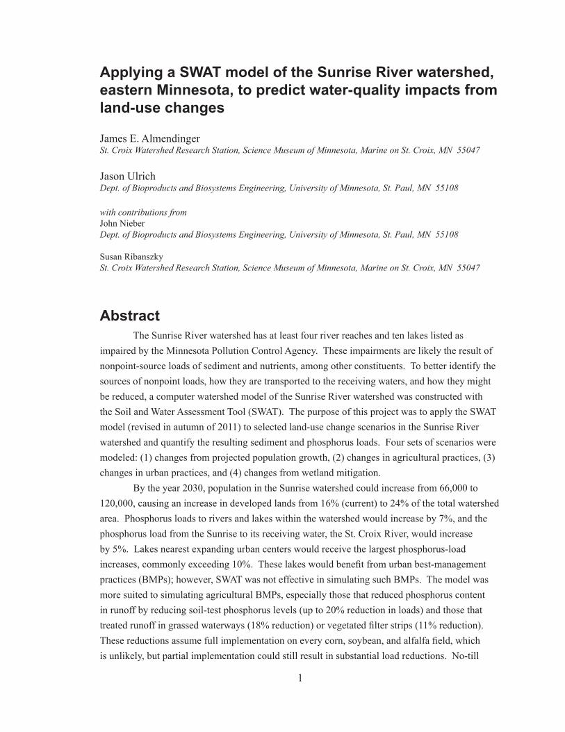
AbstractThe Sunrise River watershed has at least four river reaches and ten lakes listed as
impaired by the Minnesota Pollution Control Agency. These impairments are likely the result of nonpoint-source loads of sediment and nutrients, among other constituents. To better identify the sources of nonpoint loads, how they are transported to the receiving waters, and how they might be reduced, a computer watershed model of the Sunrise River watershed was constructed with the Soil and Water Assessment Tool (SWAT). The purpose of this project was to apply the SWAT model (revised in autumn of 2011) to selected land-use change scenarios in the Sunrise River watershed and quantify the resulting sediment and phosphorus loads. Four sets of scenarios were modeled: (1) changes from projected population growth, (2) changes in agricultural practices, (3) changes in urban practices, and (4) changes from wetland mitigation.
By the year 2030, population in the Sunrise watershed could increase from 66,000 to 120,000, causing an increase in developed lands from 16% (current) to 24% of the total watershed area. Phosphorus loads to rivers and lakes within the watershed would increase by 7%, and the phosphorus load from the Sunrise to its receiving water, the St. Croix River, would increase by 5%. Lakes nearest expanding urban centers would receive the largest phosphorus-load increases, commonly exceeding 10%. These lakes would benefit from urban best-management practices (BMPs); however, SWAT was not effective in simulating such BMPs. The model was more suited to simulating agricultural BMPs, especially those that reduced phosphorus content in runoff by reducing soil-test phosphorus levels (up to 20% reduction in loads) and those that treated runoff in grassed waterways (18% reduction) or vegetated filter strips (11% reduction). These reductions assume full implementation on every corn, soybean, and alfalfa field, which is unlikely, but partial implementation could still result in substantial load reductions. No-till
2
scenarios were much more effective at reducing sediment loads than phosphorus. Wetland restoration or routing more runoff through existing wetlands could result in substantial phosphorus load reductions, up to nearly 20% at the watershed outlet and within the Chisago Lakes Improvement District.
Overall we conclude that reducing nonpoint loads of phosphorus is feasible, but that there is no easy solution. To attain the largest reductions in phosphorus load would require substantial land modification, either as agricultural BMPs or wetland restoration, or both. The highly valued lakes adjacent to developed areas would benefit from all BMPs in their contributing areas, especially in the face of projected increases in population and development pressure. Even if these increases do not occur by the year 2030, we presume they will occur eventually.
3
Introduction
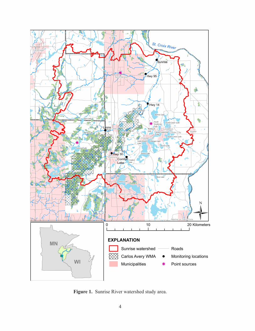
ProblemThe Sunrise River watershed comprises an area of about 991 km2 within Chisago,
Anoka, Isanti, and Washington counties in eastern Minnesota (Figure 1). The watershed contains at least four river reaches and ten lakes listed as impaired by the Minnesota Pollution Control Agency (MPCA). Listed impairments were related to turbidity, dissolved oxygen, fish diversity, invertebrate diversity, pH, and fecal coliform. In addition, among the principal tributaries to the St. Croix River, Lenz et al. (2003) identified the Sunrise River as one of the most significant contributors of phosphorus and sediment. Even though the St. Croix River has been federally recognized for its scenic beauty and recreational value, both Minnesota and Wisconsin have listed the lowermost 40 km of the St. Croix River as impaired because of excessive phosphorus and have stated a goal to reduce phosphorus loads by 20% relative to those of the 1990s (SCBWRPT, 2004).
Most of the impairment in the Sunrise watershed is likely caused by nonpoint-source (NP-S) pollution arising from land-use practices scattered across the landscape, especially since improvements to the Chisago Lakes and North Branch wastewater treatment plants have reduced point-source loads in recent years. Monitoring data are currently being collected to help determine the spatial pattern of NP-S loads across the watershed. These efforts involve an interagency consortium including the MPCA, Chisago County and its Soil and Water Conservation District (Chisago SWCD), Comfort Lake-Forest Lake Watershed District (CLFLWD), and the U.S. Army Corps of Engineers (USACE). In particular, the USACE is partnering with Chisago County to develop a watershed management plan that includes not only water-quality monitoring but also an assessment of channel stability and potential sites for wetland restoration.
To help translate these monitoring data into a more mechanistic understanding of the source and transport of NP-S pollutants, the St. Croix Watershed Research Station (SCWRS) has constructed a computer model to simulate the hydrology of the Sunrise River watershed (Almendinger and Ulrich, 2010), with funding from the MPCA and the National Park Service. We chose to construct the model with the Soil and Water Assessment Tool (SWAT). SWAT (Arnold and others, 1998) was developed by the U.S. Dept. of Agriculture’s Agricultural Research Service (USGS/ARS) “to predict the impact of land management practices on water, sediment and agricultural chemical yields in large, complex watersheds with varying soils, land use, and management conditions over long periods of time” (Neitsch et al., 2011). SWAT’s strength is in modeling rural landscapes, particularly agricultural land use. The model does a good job simulating rural hydrology and loads of sediment and phosphorus delivered to the receiving channel. However, SWAT has limited ability to simulate in-channel and in-lake processes; other models should be considered for these processes. Further, while SWAT has the capability to model urban landscapes, these routines have not been well-tested in the literature. Nonetheless, cautious interpretation of model output should still provide useful information to watershed
4
k
k
k
Coon Lake
Forest Lake
Green Lake
Sunrise Lake
South Center Lake
Linwood Lake
North Center Lake
North Pool
South Pool South LindstromLake
Typo Lake
Chisago Lake
Martin Lake
ComfortLake
Little GreenLake
Bone Lake
NorthLindstromLake
Kroon Lake
WallmarkLake
St. Croix River
East Bethel
Ham Lake
Harris
Forest Lake
North Branch
santi
Stacy
Cambridge
Wyoming
Lindstrom
Marine on Saint Croix
Chisago City
Shafer
ridge
Center City
0 10 20 KilometersÜ
MN
WI
EXPLANATION
Roads
Monitoring locations
k Point sources
Sunrise watershed
Carlos Avery WMA
Municipalities
Sunrise
Hwy 95
Hwy 14
Lyons
Hwy 30ComfortLake
figure 1. Sunrise River watershed study area.
5
managers, and testing such routines will ultimately help improve the model itself. Overall, SWAT remains one of the best tools available for simulating whole-watershed loads of NP-S pollutants.
Purpose and ScopeThis report describes the application of the Sunrise River watershed SWAT model to
selected potential land-cover and land-management scenarios to predict the resulting changes in NP-S loads occurring within the watershed and ultimately entering the St. Croix. The watershed model as calibrated and validated to 1999-2009 data sets served as the initial baseline against which all other model runs were contrasted. Four sets of scenarios were modeled: (1) changes from projected population growth, (2) changes in agricultural practices, (3) changes in urban practices, and (4) changes from wetland mitigation. Because of model limitations, not all these scenarios can be modeled with equal confidence. In particular, simulations of urban, in-channel, and in-lake processes are currently limited.
Details of how the Sunrise SWAT model was constructed are given in Almendinger and Ulrich (2010). However, that report describes the model as constructed for the SWAT2005 program, which has been superseded by SWAT2009. The Sunrise model was updated and recalibrated for SWAT2009 in the fall of 2011. The reconfigured model was broadly similar to the original, but with some notable differences. In the original model, channel erosion was the dominant source of suspended sediment reaching the watershed outlet, and groundwater was the largest source of phosphorus. In the SWAT2009 version, channel erosion was a co-equal source of sediment (46% of the total) and groundwater was a minor contributor of phosphorus (10% of the total). Details for SWAT parameters mentioned in this report (typically written in all capitals) can be found in the SWAT user’s guide (Arnold et al., 2011).
Scenario Set 1: Changes from projected population growth
We distinguish here a conceptual difference between “what-if” scenarios, and “what-when” scenarios. A “what-if” scenario describes a possible – but by no means certain -- future configuration of land cover, land use, climate, and so forth in a watershed. We may or may not change certain agricultural practices, we may or may not restore some wetlands, and local climate may or may not change significantly. However, because population has nearly always grown throughout history, and because most of this growth now occurs in cities and urban fringes, population projections have an air of inevitability about them. The question is generally not if but when population will grow, thereby consuming land for residential and commercial uses. Hence we treat population projections as “what-when” scenarios that form “future baselines” for further what-if scenarios. We note, however, that even in the face of probable population growth,
6
land managers may have substantial discretion about how land is developed to accommodate this growth.
The goal of this modeling task was to predict the changes in water-quality resulting from changes in land-cover and waste-water loads as a consequence of projected population increases in the Sunrise River watershed. We chose to include population projections for two time slices, 2020 and 2030. Configuring the model for these projected runs required three steps: acquisition of population growth projections, calculation of increased waste-water loads, and estimation of increased developed land cover. Each model configuration (2000s, 2020, and 2030) was run for a 30-year period using precipitation and temperature data for 1980-2009. The first 10 years of model output were ignored to allow model equilibration, and the last 20 years were averaged to obtain typical yields and loads of sediment and phosphorus for each model configuration.
LentTownship
Forest LakeCity
North BranchCity
LinwoodTownship
New ScandiaTownship
WyomingTownship
OxfordTownship
SunriseTownship
Chisago LakeTownship
North BranchTownship
WyomingCity
StacyCity
CenterCity
ChisagoCity
LindstromCity
0 10 205 Kilometers
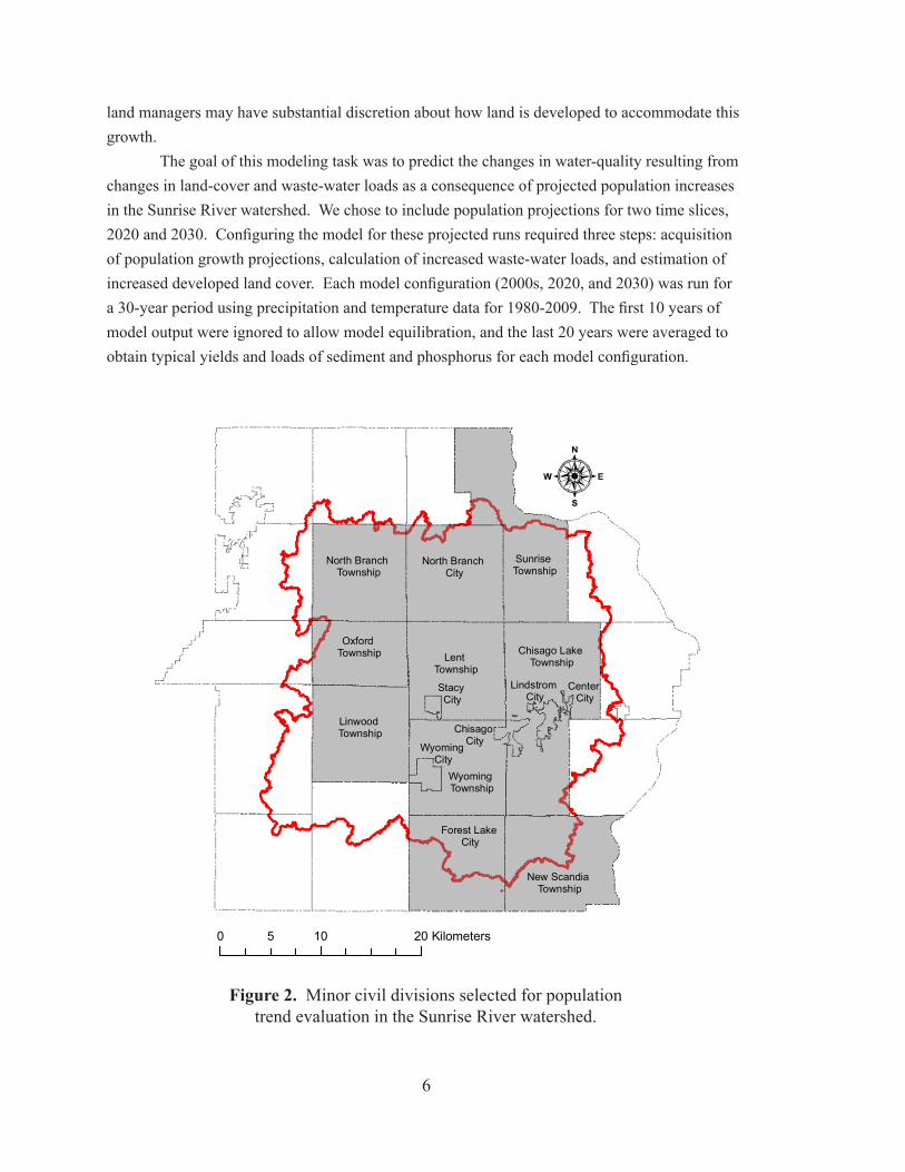
figure 2. Minor civil divisions selected for population trend evaluation in the Sunrise River watershed.
7
Population GrowthPopulation data were available for minor civil divisions (MCDs) in and adjacent to the
watershed. We chose to analyze those MCDs whose centroids lay within the watershed boundary (Figure 2). The aggregate area of these MCDs is similar to that of the watershed, and we presume the population in these MCDs is representative of that in the watershed. These MCDs include seven cities and eight townships. North Branch City and Forest Lake City are somewhat hybrids, in the sense that the city boundaries extend to the full area of a township but the urban core occupies only part of the area and a substantial portion retains a semi-rural character.
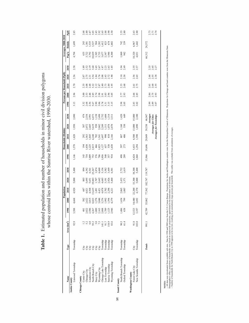
Decadal population and household data are given in Table 1 for each MCD. Data for 1990 and 2000 were obtained from the U.S. Census Bureau. Projected data for 2010, 2020, and 2030 were obtained from the Metropolitan Council for Anoka and Washington counties, and from the Minnesota State Demographer’s office for Chisago and Isanti counties. Average data for 2000-2010 were used to represent current conditions in the SWAT model, and data for 2020 and 2030 were chosen to represent future conditions. These data suggest that the total population in these MCDs will increase from about 78,000 in 2010 to 103,000 in 2020 (a 32% increase) and to 120,000 in 2030 (54% increase from 2010). Given the general economic slow-down since 2008, these growth predictions seem large. However, we presume they will eventually be achieved at some time in the future, if not by 2020 and 2030.
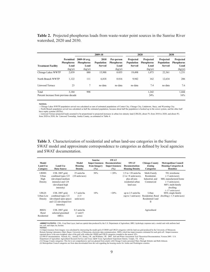
Waste-Water LoadsThere are three permitted waste-water treatment point sources in the watershed (Table 2).
Chisago Lakes Waste-Water Treatment Plant (WWTP) in Chisago Lake Township is the largest and serves the cities of Center City, Chisago, Lindstrom, Stacy, and Wyoming. North Branch WWTP serves the city of North Branch. A small population in Linwood Township is served by a wetland seepage system with very small discharge loads. Waste-water loads were presumed to increase on a linear per-capita basis from current loads. Current loads were determined from the most recent data available (2009-10), rather than as a decadal average over 2000-10, in order to account for improvements in treatment technology attained during the past few years that should carry forward to future operations. Increases in the population served by these WWTPs would increase point-source phosphorus loads by 24% from 2010 to 2020, and by 16% from 2020 to 2030. According to these projections, the total annual phosphorus load of 1444 kg from these three sources in 2030 would still be significantly below the permitted total annual load of 3184 kg.
Increases in Residential Land CoverDetermining the increase in residential land cover due to population growth required
several steps. First, what are the housing densities (households per unit land area) for the
8
Nam
eT
ype
Are
a (k
m2 )
1990
2000
2010
2020
2030
1990
2000
2010
2020
2030
1990
2000
2010
2020
2030
Pop'
nH
shld
sPp
HA
noka
Cou
nty
Linw
ood
Tow
nshi
pTo
wns
hip
92.9
3,58
84,
668
4,92
05,
000
5,40
01,
146
1,57
81,
820
1,95
02,
090
3.13
2.96
2.70
2.56
2.58
4,79
41,
699
2.83
Chi
sago
Cou
nty
Cen
ter C
ityC
ity1.
248
158
268
780
389
414
519
429
238
747
43.
323.
002.
352.
071.
8963
524
32.
68C
hisa
go C
ityC
ity5.
22,
022
2,62
24,
821
5,69
56,
392
754
1,03
81,
563
2,07
22,
534
2.68
2.53
3.08
2.75
2.52
3,72
21,
301
2.80
Lind
stro
m C
ityC
ity6.
02,
586
3,01
54,
568
5,65
16,
541
1,00
91,
225
1,84
52,
445
2,99
12.
562.
462.
482.
312.
193,
792
1,53
52.
47N
orth
Bra
nch
City
City
93.2
4,26
78,
023
13,6
3519
,883
25,2
6775
22,
815
4,24
05,
619
6,87
35.
672.
853.
223.
543.
6810
,829
3,52
73.
03St
acy
City
City
3.0
1,08
91,
278
1,49
11,
707
1,87
437
646
670
293
01,
138
2.90
2.74
2.12
1.84
1.65
1,38
558
42.
43W
yom
ing
City
City
7.5
2,16
33,
048
4,42
15,
642
6,66
070
61,
023
1,54
12,
042
2,49
83.
062.
982.
872.
762.
673,
735
1,28
22.
92C
hisa
go L
ake
Tow
nshi
pTo
wns
hip
141.
12,
888
3,27
64,
078
4,68
55,
156
1,05
61,
127
1,69
72,
249
2,75
22.
742.
912.
402.
081.
873,
677
1,41
22.
65Le
nt T
owns
hip
Tow
nshi
p91
.71,
789
1,99
22,
702
3,19
13,
582
540
657
990
1,31
11,
604
3.31
3.03
2.73
2.43
2.23
2,34
782
32.
88Su
nris
e To
wns
hip
Tow
nshi
p11
8.9
1,12
51,
594
2,29
82,
926
3,44
935
753
881
01,
074
1,31
43.
152.
962.
842.
722.
631,
946
674
2.90
Wyo
min
g To
wns
hip
Tow
nshi
p83
.62,
946
4,37
94,
221
5,46
06,
501
934
1,43
82,
166
2,87
03,
511
3.15
3.05
1.95
1.90
1.85
4,30
01,
802
2.50
Isan
ti C
ount
yN
orth
Bra
nch
Tow
nshi
pTo
wns
hip
90.5
1,48
61,
654
2,06
52,
433
2,75
249
859
788
71,
160
1,42
02.
982.
772.
332.
101.
941,
860
742
2.55
Oxf
ord
Tow
nshi
pTo
wns
hip
61.4
638
799
1,08
51,
371
1,61
920
927
340
653
064
93.
052.
932.
682.
582.
4994
233
92.
80
Was
hing
ton
Cou
nty
Fore
st L
ake
City
City
91.8
12,5
2314
,440
22,2
0033
,300
38,3
004,
424
5,43
38,
500
13,0
0015
,000
2.83
2.66
2.61
2.56
2.55
18,3
206,
967
2.63
New
Sca
ndia
Tow
nshi
pTo
wns
hip
103.
03,
197
3,69
24,
370
5,00
05,
400
1,06
01,
294
1,59
01,
890
2,10
03.
022.
852.
752.
652.
574,
031
1,44
22.
80
Tota
ls99
1.1
42,7
8955
,062
77,5
6210
2,74
711
9,78
713
,966
19,6
9629
,049
39,5
3046
,947
66,3
1224
,372
Aver
ages
2.99
2.84
2.61
2.46
2.35
2.73
Aver
ages
for C
ities
2.89
2.75
2.68
2.55
2.45
2.71
Aver
ages
for T
owns
hips
3.07
2.93
2.55
2.38
2.27
2.74
Popu
latio
nH
ouse
hold
s (H
shld
s)Pe
rson
s per
Hou
seho
ld (P
pH)
Ave
rage
s, 20
00-2
010
NO
TE
S:--
All
data
wer
e do
wnl
oade
d fr
om a
vaila
ble
web
site
s. D
ata
for 1
990
and
2000
wer
e fr
om th
e U
.S. C
ensu
s B
urea
u. P
roje
ctio
ns f
orA
noka
and
Was
hing
ton
coun
ties
wer
e fr
om th
e M
etro
polit
an C
ounc
il of
Min
neso
ta.
Proj
ectio
ns f
or C
hisa
go a
nd Is
anti
coun
ties
wer
e fr
om th
e M
inne
sota
Sta
te
Dem
ogra
pher
's of
fice;
pro
ject
ions
of h
ouse
hold
s w
ere
base
d on
cou
ntyw
ide
proj
ectio
ns, a
ppor
tione
d to
the
liste
d m
inor
civ
il di
visi
ons.
--
Num
ber o
f hou
seho
lds
for N
orth
Bra
nch
City
in 1
990
appe
ars t
o be
too
low
, res
ultin
g in
an
anom
alou
sly
larg
e pe
rson
s per
hou
seho
ld.
This
out
lier w
as e
xclu
ded
from
cal
cula
tions
of a
vera
ges.
Tabl
e 1.
Est
imat
ed p
opul
atio
n an
d nu
mbe
r of h
ouse
hold
s in
min
or c
ivil
divi
sion
pol
ygon
s w
hose
cen
troid
lies
with
in th
e Su
nris
e R
iver
wat
ersh
ed, 1
990-
2030
.
9
Treatment Facility
PermittedPhosphorus
Load
2009-10 avg.Phosphorus
Load
2010Population
Served
Per-personPhosphorus
Load
ProjectedPopulation
Served
ProjectedPhosphorus
Load
ProjectedPopulation
Served
ProjectedPhosphorus
Load(kg/yr) (kg/yr) (kg/yr) (kg/yr) (kg/yr)
Chisago Lakes WWTP 2,039 880 15,988 0.055 19,498 1,073 22,361 1,231
North Branch WWTP 1,122 111 6,818 0.016 9,942 162 12,634 206
Linwood Terrace 23 7 no data no data no data 7.4 no data 7.6
Total 3,184 998 1,242 1,444Percent increase from previous decade 24% 16%
2009-10 2020 2030
NOTES:-- Chisago Lakes WWTP population served was calculated as sum of estimated populations of Center City, Chisago City, Lindstrom, Stacy, and Wyoming City. -- North Branch population served was calculated as half the estimated population, because about half the population is hooked up to the sewer system, and the other half have septic systems (ISTSs). -- Linwood Terrace projected loads assumed to be proportional to projected increases in urban low-density land (URLD), about 5% from 2010 to 2020, and about 4% from 2020 to 2030, for Linwood Township, Anoka County, as estimated in Table 4.
Table 2. Projected phosphorus loads from waste-water point sources in the Sunrise River watershed, 2020 and 2030.
Model Land-UseCategory
Land-UseData Source
Model Housing Density
SunriseImperviousnessfrom Imagery
(%)
SWAT Documentation: Imperviousness
(%)
SWAT Documentation: Housing Density
Chisago County Zoning
Categories
Metropolitan CouncilHousing Categories &
Densities
URHD: Urban High
Density
CDL 2007 grid; combined types 123 (developed medium intensity) and 124 (developed high
intensity)
25 units/ha(10 units/acre)
50% > 20% 2.5 to >20 units/ha(1 to >8 units/acre),
plus all non-residential urban
land uses
Multi-Family Residential,
Industrial, and Commercial
TH, townhome (~5 units/acre);
MH, manufactured home (~5 units/acre);
MF5, multi-family dwelling
(~17 units/acre)URLD:
Urban Low Density
CDL 2007 grid; combined types 121
(developed open space) and 122 (developed low
intensity)
3.7 units/ha(1.5
units/acre)
10% <20% up to 2.5 units/ha(up to 1 unit/acre)
Urban Residential, Rural Residential I and
II
SFD, single-family dwelling (~1.5 units/acre)
RRES: Rural
Residential
CDL 2007 grid; selected grassland
HRUs
0.5 units/ha(1 unit/5
acres)
Agricultural
ABBREVIATIONS: CDL, Crop Data Layer, land-use spatial data produced by the U.S. Department of Agriculture; HRU, hydrologic response unit, a model unit with uniform land use, soil, and slope; ha, hectare.NOTES:(1) Imperviousness from imagery was calculated by intersecting the model grid of URHD and URLD categories with the land-use grid produced by the University of Minnesota Remote Sensing Laboratory (Marv Bauer, University of Minnesota, electronic data communication, 2009), which has imperviousness estimated for each grid cell. Iimperviousness reported above is the area-weighted value of the grid cells within the URHD and URLD categories rounded to the nearest 10%. (2) SWAT documentation: Neitsch, S.L., Arnold, J.G., Kiniry, J.R., and Williams, J.R. 2005. Soil and Water Assessment Tool Theoretical Documentation, Version 2005. U.S. Department of Agriculture Agricultural Research Service and Texas A&M Texas Agricultural Experiment Station, Temple, TX. 476 p.(3) Chisago County categories: This list is not comprehensive and was gleaned from emails with Chisago County personnel Mary Darragh Schmitz and Beth Johnson. (4) Metropolitan Council categories are from data downloaded from the web regarding the housing stocks for Anoka and Washington counties.
Table 3. Characterization of residential and urban land-use categories in the Sunrise SWAT model and approximate correspondence to categories as defined by local agencies and SWAT documentation.
10
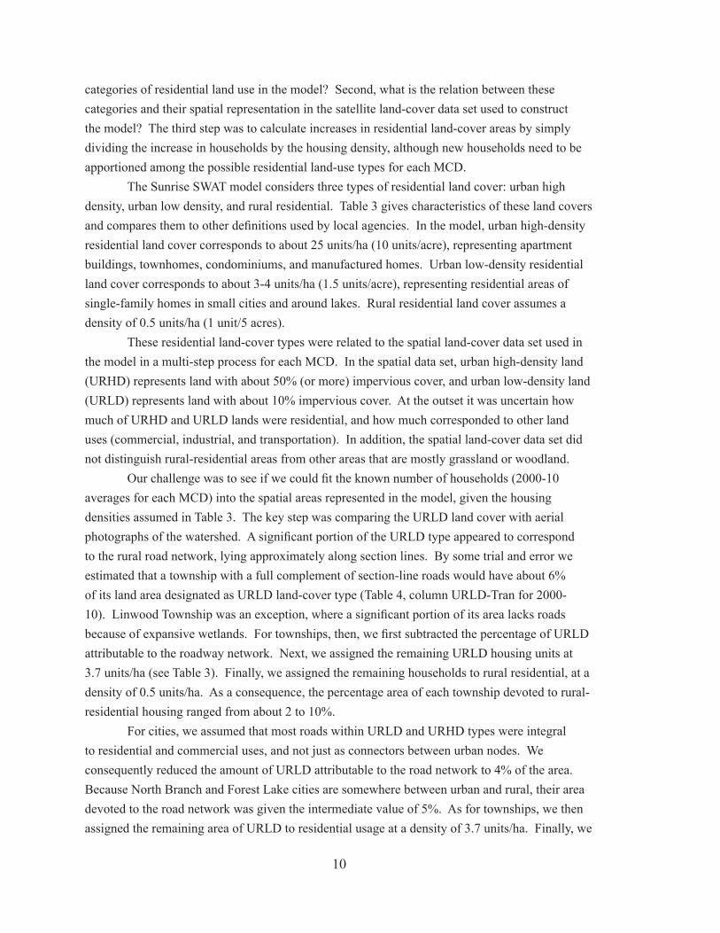
categories of residential land use in the model? Second, what is the relation between these categories and their spatial representation in the satellite land-cover data set used to construct the model? The third step was to calculate increases in residential land-cover areas by simply dividing the increase in households by the housing density, although new households need to be apportioned among the possible residential land-use types for each MCD.
The Sunrise SWAT model considers three types of residential land cover: urban high density, urban low density, and rural residential. Table 3 gives characteristics of these land covers and compares them to other definitions used by local agencies. In the model, urban high-density residential land cover corresponds to about 25 units/ha (10 units/acre), representing apartment buildings, townhomes, condominiums, and manufactured homes. Urban low-density residential land cover corresponds to about 3-4 units/ha (1.5 units/acre), representing residential areas of single-family homes in small cities and around lakes. Rural residential land cover assumes a density of 0.5 units/ha (1 unit/5 acres).
These residential land-cover types were related to the spatial land-cover data set used in the model in a multi-step process for each MCD. In the spatial data set, urban high-density land (URHD) represents land with about 50% (or more) impervious cover, and urban low-density land (URLD) represents land with about 10% impervious cover. At the outset it was uncertain how much of URHD and URLD lands were residential, and how much corresponded to other land uses (commercial, industrial, and transportation). In addition, the spatial land-cover data set did not distinguish rural-residential areas from other areas that are mostly grassland or woodland.
Our challenge was to see if we could fit the known number of households (2000-10 averages for each MCD) into the spatial areas represented in the model, given the housing densities assumed in Table 3. The key step was comparing the URLD land cover with aerial photographs of the watershed. A significant portion of the URLD type appeared to correspond to the rural road network, lying approximately along section lines. By some trial and error we estimated that a township with a full complement of section-line roads would have about 6% of its land area designated as URLD land-cover type (Table 4, column URLD-Tran for 2000-10). Linwood Township was an exception, where a significant portion of its area lacks roads because of expansive wetlands. For townships, then, we first subtracted the percentage of URLD attributable to the roadway network. Next, we assigned the remaining URLD housing units at 3.7 units/ha (see Table 3). Finally, we assigned the remaining households to rural residential, at a density of 0.5 units/ha. As a consequence, the percentage area of each township devoted to rural-residential housing ranged from about 2 to 10%.
For cities, we assumed that most roads within URLD and URHD types were integral to residential and commercial uses, and not just as connectors between urban nodes. We consequently reduced the amount of URLD attributable to the road network to 4% of the area. Because North Branch and Forest Lake cities are somewhere between urban and rural, their area devoted to the road network was given the intermediate value of 5%. As for townships, we then assigned the remaining area of URLD to residential usage at a density of 3.7 units/ha. Finally, we
11
RR
ES
UR
HD
UR
LD
RR
ES
RR
ES
Nam
eT
ype
Are
a 20
00-1
020
2020
30C
omR
esT
ran
Res
Res
Vac
Vac
Com
Res
Tra
nR
esR
esC
omR
esT
ran
Res
Res
(km
2 )(%
are
a)(%
are
a)(%
are
a)(%
are
a)(%
are
a)(%
are
a)(%
are
a)(%
are
a)(%
are
a)(%
are
a)(%
are
a)(%
are
a)(%
are
a)(%
are
a)(%
are
a)(%
are
a)(%
are
a)A
noka
Cou
nty
Linw
ood
Tow
nshi
p92
.91,
699
1,95
02,
090
0.0
0.0
3.0
3.6
10.1
ndnd
0.0
0.0
3.0
3.9
11.6
0.0
0.0
3.0
4.2
12.4
Chi
sago
Cou
nty
Cen
ter C
ityC
ity1.
224
338
747
47.
83.
34.
030
.40.
00.
00.
512
.45.
34.
047
.90.
015
.26.
54.
058
.60.
0C
hisa
goC
ity5.
21,
301
2,07
22,
534
9.7
4.3
4.0
38.2
0.0
0.4
2.0
15.3
6.8
4.0
58.8
0.0
18.7
8.3
4.0
72.0
0.0
Lind
stro
mC
ity6.
01,
535
2,44
52,
991
10.0
3.4
4.0
46.4
0.0
0.8
2.8
15.3
5.2
4.0
71.2
0.0
18.7
6.4
4.0
87.1
0.0
Nor
th B
ranc
hC
ity93
.23,
527
5,61
96,
873
1.6
0.4
5.0
7.9
16.6
0.1
0.2
2.5
0.7
5.0
12.3
26.5
3.1
0.8
5.0
15.0
32.4
Stac
yC
ity3.
058
493
01,
138
12.9
3.4
4.0
30.1
0.0
0.6
2.3
20.1
5.3
4.0
45.6
0.0
24.6
6.4
4.0
55.8
0.0
Wyo
min
gC
ity7.
51,
282
2,04
22,
498
12.5
2.2
4.0
31.2
0.0
0.5
1.5
19.5
3.4
4.0
48.2
0.0
23.8
4.2
4.0
59.0
0.0
Chi
sago
Lak
eTo
wns
hip
141.
11,
412
2,24
92,
752
0.0
0.0
6.0
2.1
4.1
0.0
0.3
0.0
0.0
6.0
3.1
6.5
0.0
0.0
6.0
3.8
8.0
Lent
Tow
nshi
p91
.782
31,
311
1,60
40.
00.
06.
01.
75.
10.
00.
10.
00.
06.
02.
78.
10.
00.
06.
03.
310
.0Su
nris
eTo
wns
hip
118.
967
41,
074
1,31
40.
00.
06.
02.
70.
00.
00.
10.
00.
06.
04.
20.
00.
00.
06.
05.
20.
0W
yom
ing
Tow
nshi
p83
.61,
802
2,87
03,
511
0.0
0.0
6.0
4.4
10.3
0.0
0.3
0.0
0.0
6.0
6.8
16.4
0.0
0.0
6.0
8.3
20.1
Isan
ti C
ount
yN
orth
Bra
nch
Tow
nshi
p90
.574
21,
160
1,42
00.
00.
06.
02.
01.
9nd
nd0.
00.
06.
02.
93.
00.
00.
06.
03.
53.
7O
xfor
dTo
wns
hip
61.4
339
530
649
0.0
0.0
4.0
0.6
6.3
ndnd
0.0
0.0
4.0
0.7
9.9
0.0
0.0
4.0
0.9
12.1
Was
hing
ton
Cou
nty
Fore
st L
ake
City
91.8
6,96
713
,000
15,0
003.
70.
55.
013
.50.
0nd
nd6.
50.
95.
023
.60.
07.
51.
05.
027
.20.
0N
ew S
cand
iaTo
wns
hip
103.
01,
442
1,89
02,
100
0.0
0.0
6.0
2.8
2.5
ndnd
0.0
0.0
6.0
3.4
3.3
0.0
0.0
6.0
3.8
3.6
Totals
991.
124
,372
39,5
3046
,947
UR
LD
2000
-10
aver
age
2020
2030
2010
Hou
seho
lds
UR
HD
UR
LD
UR
HD
UR
LD
UR
HD
AB
BR
EV
IAT
ION
S:U
RH
D, u
rban
hig
h de
nsity
; UR
LD, u
rban
low
den
sity
; RR
ES, r
ural
resi
dent
ial;
Com
, com
mer
cial
and
othe
r non
-res
iden
tial u
rban
land
use
; Res
, res
iden
tial;
Tran
, tra
nspo
rtatio
n; V
ac, v
acan
t; nd
, no
data
; km
2 , sq
uare
kilo
met
ers.
N
OT
ES:
Min
or c
ivil
divi
sion
s inc
lude
d ar
e th
ose
who
se c
entro
id fa
lls w
ithin
the
Sunr
ise
wat
ersh
ed.
Vac
ant u
rban
land
det
erm
ined
as th
e in
ters
ectio
n of
cur
rent
vac
ant p
arce
ls (B
eth
John
son,
GIS
spec
ialis
t, C
hisa
go C
ount
y, e
lect
roni
c dat
a co
mm
unic
atio
n, Ju
ly 2
010)
w
ith d
evel
oped
land
in th
e 20
07 C
rop
Dat
a La
yer,
the
prin
cipa
l lan
d-us
e dat
a in
put t
o th
e SW
AT
mod
el.
Dev
elop
ed o
pen
and
low
-inte
nsity
land
s wer
e as
sign
ed to
UR
LD, a
nd d
evel
oped
med
ium
-and
hig
h-in
tens
ity la
nds w
ere
assi
gned
to U
RH
D.
For c
urre
nt (2
000-
10 av
erag
e) c
onfig
urat
ion,
the
first
6%
of U
RLD
in to
wns
hips
was
ass
igne
d to
tran
spor
tatio
n to
acc
ount
for t
he e
xist
ing
road
net
wor
k (th
e se
ctio
n-lin
e fra
mew
ork)
, with
a fe
w e
xcep
tions
(Lin
woo
d an
d O
xfor
d to
wns
hips
) whe
re la
rge
wet
land
s re
duce
d ro
ad n
etw
ork
dens
ity.
In c
ities
, the
firs
t 4%
of U
RLD
was
ass
igne
d to
the
trans
porta
tion
netw
ork.
The
rem
aini
ng U
RL
D in
bot
h to
wns
hips
and
citie
s was
ass
igne
d to
resi
dent
ial l
and
with
3.7
hou
seho
ld u
nits
/ha (
1.5
units
/acr
e).
In to
wns
hips
, the
rem
aini
ng
hous
ehol
ds w
ere
then
ass
igne
d to
RR
ES, a
t 0.5
uni
ts/h
a (1
uni
t / 5
acr
es).
In c
ities
, the
rem
aini
ng h
ouse
hold
s wer
e as
sign
edto
UR
HD
resi
dent
ial,
at 2
5 ho
useh
old
units
/ha
(10
units
/acr
e), w
ith th
e re
mai
ning
UR
HD
land
ass
igne
d to
com
mer
cial
pur
pose
s.
For 2
020
proj
ecte
d co
nfig
urat
ion,
UR
LD-T
ran
(the
basi
c ro
ad fr
amew
ork)
was
ass
umed
to re
mai
n co
nsta
nt, a
nd th
e pe
rcen
t are
as o
f UR
HD
-Com
, UR
HD
-Res
, UR
LD-R
es, a
nd R
RES
wer
e as
sum
ed to
incr
ease
the
sam
e as
the
ratio
of 2
020
hous
ehol
ds to
200
0-10
ho
useh
olds
. Th
e in
crea
ses u
rban
land
wer
e th
en re
duce
d by
the
perc
ent o
f urb
an v
acan
t lan
d (U
RH
D-V
ac &
UR
LD-V
ac),
unde
r the
ass
umpt
ion
that
this
land
wou
ld b
e us
ed fi
rst,
befo
re n
on-u
rban
land
was
dev
elop
ed.
For 2
030
proj
ecte
d co
nfig
urat
ion,
the
sam
e ru
les w
ere
appl
ied,
whe
re U
RLD
-Tra
n w
as h
eld
cons
tant
and
UR
HD
-Com
, UR
HD
-Res
, UR
LD-R
es, a
nd R
RES
per
cent
ages
wer
e in
crea
sed
from
202
0 by
the
ratio
of 2
030
to 2
020
hous
ehol
ds.
Tabl
e 4.
Res
iden
tial a
nd u
rban
land
use
in th
e m
inor
civ
il di
visi
ons i
n th
e Su
nris
e R
iver
wat
ersh
ed, b
ased
on
num
bers
of h
ouse
hold
s ap
porti
oned
am
ong
urba
n hi
gh d
ensi
ty (U
RH
D),
urba
n lo
w d
ensi
ty (U
RLD
), an
d ru
ral r
esid
entia
l (R
RES
) lan
d co
vers
, fo
r cur
rent
(200
0-10
ave
rage
) and
pro
ject
ed (2
020
and
2030
) con
figur
atio
ns.
12
assigned the remaining number of households to part of the URHD area, at a density of 25 units/ha. The remaining URHD was assumed to be for commercial or industrial use. The consequence of these calculations was that the area of commercial URHD land was about two or three times the area of residential URHD land, which in turn was only one-tenth that of residential URLD land in cities.
For projecting increased areas in 2020 (Table 4), the percent area devoted to the roadway network as presumed to stay the same. Then the residential URLD, URHD, and rural-residential areas were assumed to increase while maintaining the relative proportions among these categories. Areas of commercial URHD were increased to maintain the same proportion of commercial to residential areas. Areas of currently vacant parcels that coincided with areas already designated as URLD or URHD were subtracted from the areas of projected growth, since they would probably be infilled first. That is, urban growth that infilled existing urban areas was not counted as expanding those areas. Projections for 2030 followed the same rules, except that vacant parcels were assumed to have been entirely occupied by then.
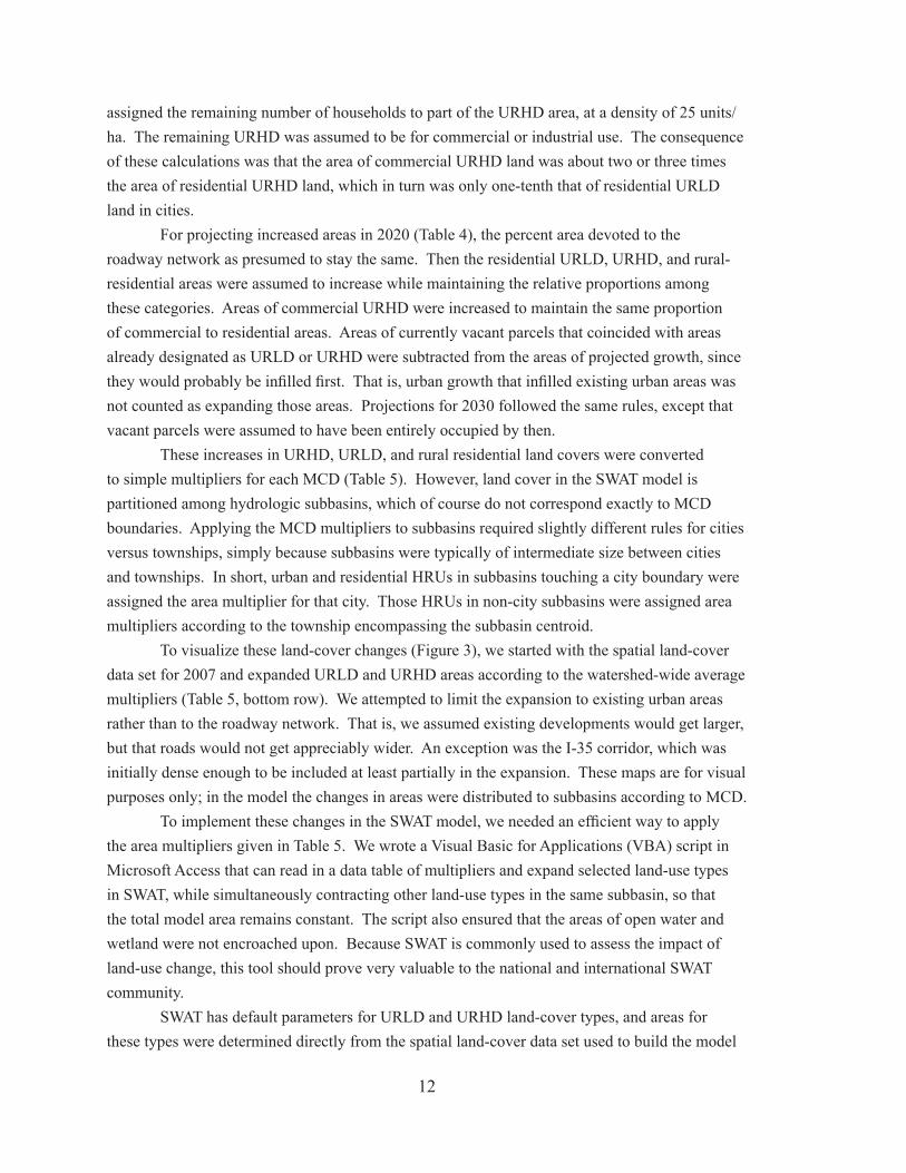
These increases in URHD, URLD, and rural residential land covers were converted to simple multipliers for each MCD (Table 5). However, land cover in the SWAT model is partitioned among hydrologic subbasins, which of course do not correspond exactly to MCD boundaries. Applying the MCD multipliers to subbasins required slightly different rules for cities versus townships, simply because subbasins were typically of intermediate size between cities and townships. In short, urban and residential HRUs in subbasins touching a city boundary were assigned the area multiplier for that city. Those HRUs in non-city subbasins were assigned area multipliers according to the township encompassing the subbasin centroid.
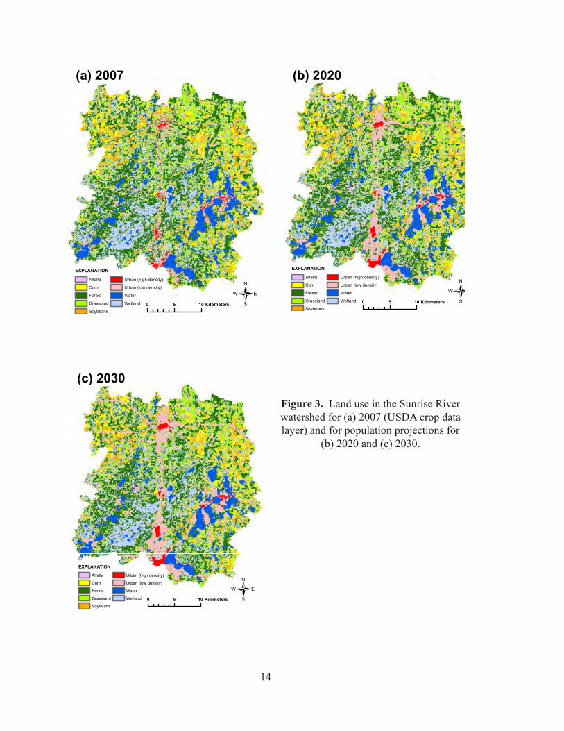
To visualize these land-cover changes (Figure 3), we started with the spatial land-cover data set for 2007 and expanded URLD and URHD areas according to the watershed-wide average multipliers (Table 5, bottom row). We attempted to limit the expansion to existing urban areas rather than to the roadway network. That is, we assumed existing developments would get larger, but that roads would not get appreciably wider. An exception was the I-35 corridor, which was initially dense enough to be included at least partially in the expansion. These maps are for visual purposes only; in the model the changes in areas were distributed to subbasins according to MCD.
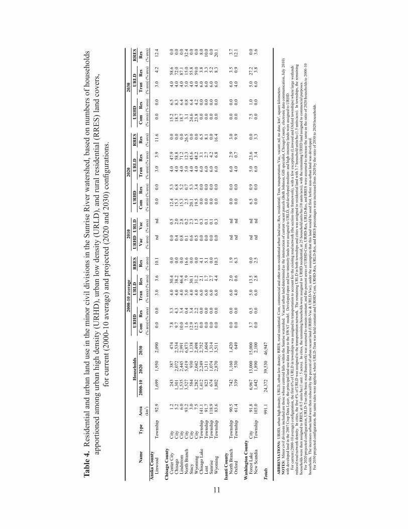
To implement these changes in the SWAT model, we needed an efficient way to apply the area multipliers given in Table 5. We wrote a Visual Basic for Applications (VBA) script in Microsoft Access that can read in a data table of multipliers and expand selected land-use types in SWAT, while simultaneously contracting other land-use types in the same subbasin, so that the total model area remains constant. The script also ensured that the areas of open water and wetland were not encroached upon. Because SWAT is commonly used to assess the impact of land-use change, this tool should prove very valuable to the national and international SWAT community.
SWAT has default parameters for URLD and URHD land-cover types, and areas for these types were determined directly from the spatial land-cover data set used to build the model
13
(the 2007 crop data layer from the USDA/NASS web site). However, rural residential (RRES) land cover was not distinguished in the spatial data set, nor does SWAT have a corresponding land-cover type in its database. Evidently, RRES lands are scattered somewhere among the lands otherwise identified as grassland or forest in the spatial data set, and these areas need to be identified and reassigned parameters characteristic of RRES land. Consequently we first selected grassland HRUs up to the total area of RRES land estimated in Table 4 for each
Area multipiers... Area multipiers...From 2000-10 to 2020 From 2020 to 2030
MCD Name URHD URLD RRES URHD URLD RRESAnoka County
Linwood Township -- 1.05 1.15 1.07 1.04 1.07
Chisago CountyCenter City 1.59 1.51 -- 1.22 1.21 --Chisago City 1.57 1.49 -- 1.22 1.21 --Lindstrom City 1.53 1.49 -- 1.22 1.21 --North Branch City 1.56 1.35 1.59 1.22 1.16 1.22Stacy City 1.55 1.46 -- 1.22 1.21 --Wyoming City 1.56 1.48 -- 1.22 1.21 --Chisago Lake Township -- 1.12 1.59 -- 1.08 1.22Lent Township -- 1.12 1.59 -- 1.07 1.22Sunrise Township -- 1.17 -- -- 1.09 --Wyoming Township -- 1.23 1.59 -- 1.12 1.22
Isanti CountyNorth Branch Township -- 1.11 1.56 1.22 1.07 1.22Oxford Township -- 1.03 1.56 1.22 1.03 1.22
Washington CountyForest Lake City 1.77 1.55 -- 1.15 1.13 --New Scandia Township -- 1.08 1.31 1.11 1.04 1.11
Watershed-wide averages 1.59 1.28 1.49 1.19 1.12 1.19
NOTES: URHD, urban high-density land use; URLD, urban low-density land use; RRES, rural residential land use. E.g., for Center City, the area URHD is expected to increase by 59% (by a factor of 1.59), from the present (2000-10) to 2020.
Table 5. Factors describing the relative increase in areas of residential and urban land use in the minor civil divisions in the Sunrise watershed from present (2000-10) to 2020 and from 2020 to 2030.
14
0 5 10 Kilometers
EXPLANATION
Alfalfa
Corn
Forest
Grassland
Soybeans
Urban (high density)
Urban (low density)
Water
Wetland 0 5 10 Kilometers
EXPLANATION
Alfalfa
Corn
Forest
Grassland
Soybeans
Urban (high density)
Urban (low density)
Water
Wetland
0 5 10 Kilometers
EXPLANATION
Alfalfa
Corn
Forest
Grassland
Soybeans
Urban (high density)
Urban (low density)
Water
Wetland
(a) 2007 (b) 2020
(c) 2030
figure 3. Land use in the Sunrise River watershed for (a) 2007 (USDA crop data layer) and for population projections for
(b) 2020 and (c) 2030.
15
MCD. If the available grassland area was not enough to account for the estimated area of RRES land, then deciduous forest HRUs were incrementally added, starting with the smaller units, to achieve the target total area. These HRUs were then parameterized to have increased runoff and greater phosphorus export than natural grassland and forest. Curve numbers were increased to halfway between the original value and the next-wetter hydrologic soil group. Soil phosphorus concentrations were increased from the default of 5 ppm to 20 ppm, which is about half of the average for agricultural land in the watershed.
Modeled Effects of Projected Population Growth
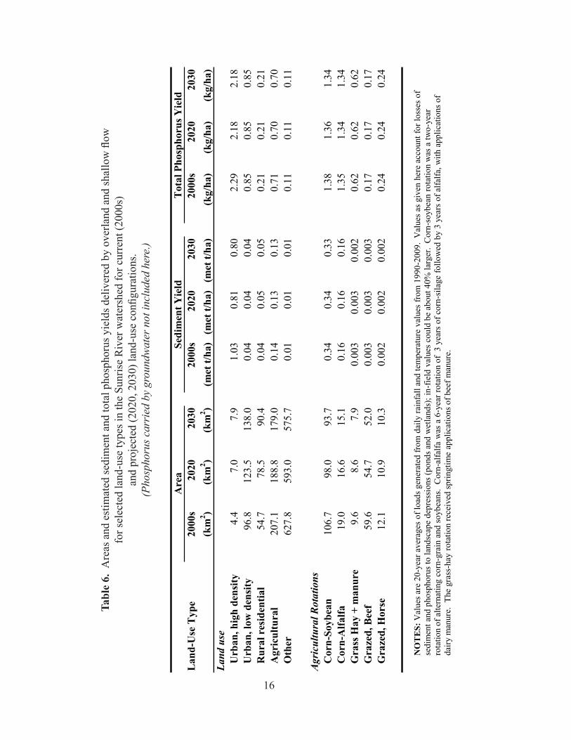
Sediment and Phosphorus Generated in HRUs and SubbasinsThe principal differences among the different model configurations was the trend of
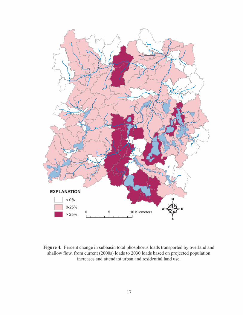
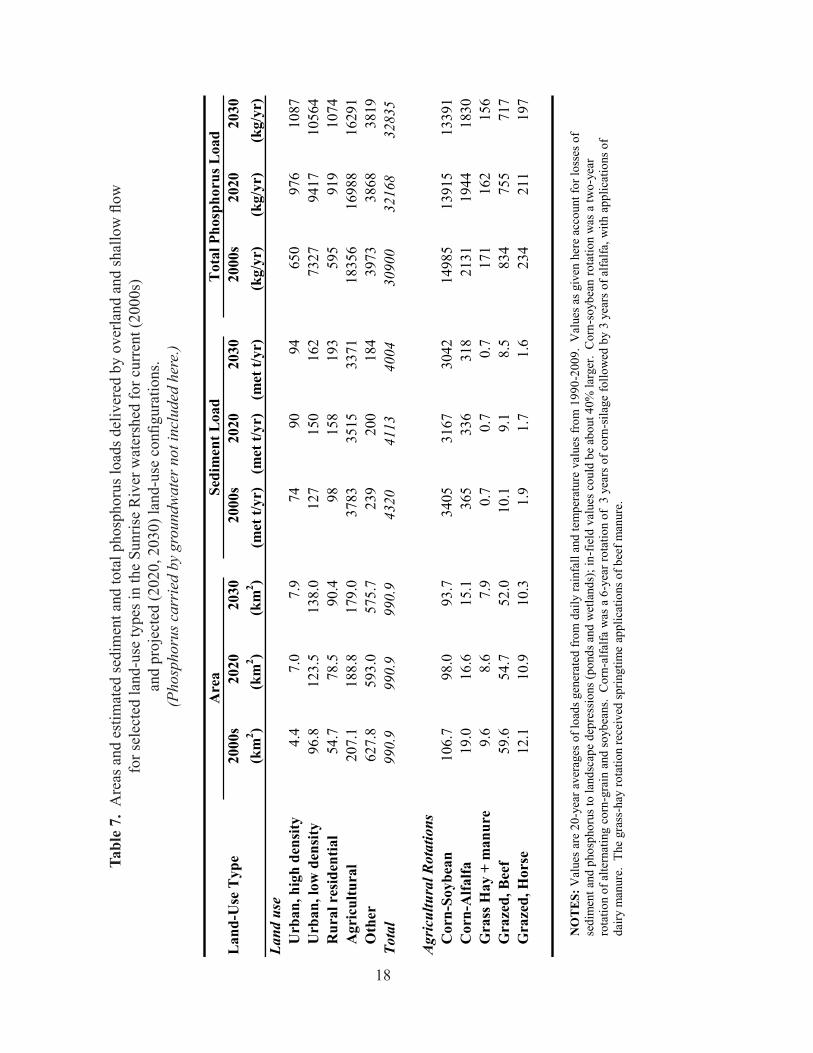
increasing area of developed land at the expense of other land-cover types, including agriculture. Urban and rural residential lands increased from 156 km2 in the 2000s configuration to 236 km2 in the 2030 configuration, while agricultural land decreased from 207 km2 to 179 km2 over the same period (Table 6). Characteristic sediment and phosphorus yields from these different land-cover types help explain the resulting changes in nonpoint-source pollutant loading. SWAT model-parameter default values resulted in high-density urban land (URHD) having the highest sediment and phosphorus yields of all land-cover types, over 0.8 t/ha sediment and about 2.2 kg/ha phosphorus (Table 6). Agricultural land, area-weighted averaged over all cropland and pastures, yielded only 0.13 t/ha sediment and 0.7 kg/ha phosphorus. Low-density urban (URLD) yielded a similar amount of phosphorus (0.85 kg/ha) but much less sediment (0.04 t/ha). Rural residential (RRES) lands yielded less sediment and phosphorus than agricultural land, but more than undeveloped land use (grassland, forest, wetland), which averaged only 0.01 t/ha sediment and 0.11 kg/ha phosphorus. For phosphorus, then, modeled yields increased in subbasins where URHD and URLD areas increased. In rural areas, phosphorus yields increased if RRES land use replaced grassland or forest but decreased where RRES replaced agricultural land (Figure 4). We caution that there is likely very large variability in actual sediment and phosphorus yields from these land-use types, and that the urban modules in SWAT have not been extensively tested in the literature, though we have no reason to dispute the results. Furthermore, the yields given here include the effect of sediment and nutrient trapping by landscape depressions specific to the Sunrise watershed, and thus they may not apply to other watersheds.
In terms of total loads generated in subbasins, agriculture contributed more sediment and phosphorus than did urban and rural residential lands (Table 7). Sediment loads were particularly dominated by agriculture, which accounted for about 85% of sediment from subbasin surfaces for all three time slices. Agriculture was also the single largest subbasin-surface source of phosphorus, but the increasing area of developed lands resulted in substantial phosphorus loads that rivaled those from agriculture. From the 2000s to 2030, the percentage of subbasin phosphorus from developed land will increase from 28% to 39%, whereas the percentage from
16
Lan
d-U
se T
ype
2000
s20
2020
3020
00s
2020
2030
2000
s20
2020
30(k
m2 )
(km
2 )(k
m2 )
(met
t/ha
)(m
et t/
ha)
(met
t/ha
)(k
g/ha
)(k
g/ha
)(k
g/ha
)La
nd u
seU
rban
, hig
h de
nsity
4.4
7.0
7.9
1.03
0.81
0.80
2.29
2.18
2.18
Urb
an, l
ow d
ensi
ty96
.812
3.5
138.
00.
040.
040.
040.
850.
850.
85R
ural
res
iden
tial
54.7
78.5
90.4
0.04
0.05
0.05
0.21
0.21
0.21
Agr
icul
tura
l20
7.1
188.
817
9.0
0.14
0.13
0.13
0.71
0.70
0.70
Oth
er62
7.8
593.
057
5.7
0.01
0.01
0.01
0.11
0.11
0.11
Agric
ultu
ral R
otat
ions
Cor
n-So
ybea
n10
6.7
98.0
93.7
0.34
0.34
0.33
1.38
1.36
1.34
Cor
n-A
lfalfa
19.0
16.6
15.1
0.16
0.16
0.16
1.35
1.34
1.34
Gra
ss H
ay +
man
ure
9.6
8.6
7.9
0.00
30.
003
0.00
20.
620.
620.
62G
raze
d, B
eef
59.6
54.7
52.0
0.00
30.
003
0.00
30.
170.
170.
17G
raze
d, H
orse
12.1
10.9
10.3
0.00
20.
002
0.00
20.
240.
240.
24
Sedi
men
t Yie
ldT
otal
Pho
spho
rus Y
ield
Are
a
NO
TES:
Val
ues a
re 2
0-ye
ar a
vera
ges
of lo
ads g
ener
ated
from
dai
ly ra
infa
ll an
d te
mpe
ratu
re v
alue
s fr
om 1
990-
2009
. V
alue
s as g
iven
her
e ac
coun
t for
loss
es o
f se
dim
ent a
nd p
hosp
horu
s to
land
scap
e de
pres
sion
s (po
nds a
nd w
etla
nds)
; in-
field
val
ues
coul
d be
abo
ut 4
0% la
rger
. C
orn-
soyb
ean
rota
tion
was
a tw
o-ye
ar
rota
tion
of a
ltern
atin
g co
rn-g
rain
and
soyb
eans
. C
orn-
alfa
lfa w
as a
6-y
ear r
otat
ion
of 3
yea
rs o
f cor
n-si
lage
follo
wed
by
3 ye
ars
of a
lfalfa
, with
app
licat
ions
of
dairy
man
ure.
The
gra
ss-h
ay ro
tatio
n re
ceiv
ed sp
ringt
ime
appl
icat
ions
of b
eef m
anur
e.
Tabl
e 6.
Are
as a
nd e
stim
ated
sedi
men
t and
tota
l pho
spho
rus y
ield
s del
iver
ed b
y ov
erla
nd a
nd sh
allo
w fl
ow
for s
elec
ted
land
-use
type
s in
the
Sunr
ise
Riv
er w
ater
shed
for c
urre
nt (2
000s
) an
d pr
ojec
ted
(202
0, 2
030)
land
-use
con
figur
atio
ns.
(Pho
spho
rus c
arri
ed b
y gr
ound
wat
er n
ot in
clud
ed h
ere.
)
17
0 5 10 Kilometers
EXPLANATION
< 0%
0-25%
> 25%
figure 4. Percent change in subbasin total phosphorus loads transported by overland and shallow flow, from current (2000s) loads to 2030 loads based on projected population
increases and attendant urban and residential land use.
18
Lan
d-U
se T
ype
2000
s20
2020
3020
00s
2020
2030
2000
s20
2020
30(k
m2 )
(km
2 )(k
m2 )
(met
t/yr
)(m
et t/
yr)
(met
t/yr
)(k
g/yr
)(k
g/yr
)(k
g/yr
)La
nd u
seU
rban
, hig
h de
nsity
4.4
7.0
7.9
7490
9465
097
610
87U
rban
, low
den
sity
96.8
123.
513
8.0
127
150
162
7327
9417
1056
4R
ural
res
iden
tial
54.7
78.5
90.4
9815
819
359
591
910
74A
gric
ultu
ral
207.
118
8.8
179.
037
8335
1533
7118
356
1698
816
291
Oth
er62
7.8
593.
057
5.7
239
200
184
3973
3868
3819
Tota
l99
0.9
990.9
990.9
4320
4113
4004
3090
032
168
3283
5
Agric
ultu
ral R
otat
ions
Cor
n-So
ybea
n10
6.7
98.0
93.7
3405
3167
3042
1498
513
915
1339
1C
orn-
Alfa
lfa19
.016
.615
.136
533
631
821
3119
4418
30G
rass
Hay
+ m
anur
e9.
68.
67.
90.
70.
70.
717
116
215
6G
raze
d, B
eef
59.6
54.7
52.0
10.1
9.1
8.5
834
755
717
Gra
zed,
Hor
se12
.110
.910
.31.
91.
71.
623
421
119
7
Are
aSe
dim
ent L
oad
Tot
al P
hosp
horu
s Loa
d
NO
TES:
Val
ues a
re 2
0-ye
ar a
vera
ges
of lo
ads g
ener
ated
from
dai
ly ra
infa
ll an
d te
mpe
ratu
re v
alue
s fr
om 1
990-
2009
. V
alue
s as g
iven
her
e ac
coun
t for
loss
es o
f se
dim
ent a
nd p
hosp
horu
s to
land
scap
e de
pres
sion
s (po
nds a
nd w
etla
nds)
; in-
field
val
ues
coul
d be
abo
ut 4
0% la
rger
. C
orn-
soyb
ean
rota
tion
was
a tw
o-ye
ar
rota
tion
of a
ltern
atin
g co
rn-g
rain
and
soyb
eans
. C
orn-
alfa
lfa w
as a
6-y
ear r
otat
ion
of 3
yea
rs o
f cor
n-si
lage
follo
wed
by
3 ye
ars
of a
lfalfa
, with
app
licat
ions
of
dairy
man
ure.
The
gra
ss-h
ay ro
tatio
n re
ceiv
ed sp
ringt
ime
appl
icat
ions
of b
eef m
anur
e.
Tabl
e 7.
Are
as a
nd e
stim
ated
sedi
men
t and
tota
l pho
spho
rus l
oads
del
iver
ed b
y ov
erla
nd a
nd sh
allo
w fl
ow
for s
elec
ted
land
-use
type
s in
the
Sunr
ise
Riv
er w
ater
shed
for c
urre
nt (2
000s
) an
d pr
ojec
ted
(202
0, 2
030)
land
-use
con
figur
atio
ns.
(Pho
spho
rus c
arri
ed b
y gr
ound
wat
er n
ot in
clud
ed h
ere.
)
19
agriculture will decrease from 59% to 50%. The above loads refer to those derived directly from the subbasin surfaces and soil layers.
Total loads leaving the watershed will be somewhat larger because of additions to sediment load from net channel erosion and to phosphorus load from groundwater discharge. In the current version of the model (built with SWAT2009), channel erosion accounted for about 46% of the total suspended sediment load leaving the watershed, and groundwater discharge accounted for about 10% of the total phosphorus load (based on a concentration of 0.02 mg/L phosphorus).
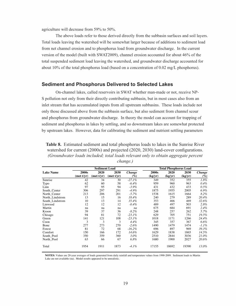
Sediment and Phosphorus Delivered to Selected LakesOn-channel lakes, called reservoirs in SWAT whether man-made or not, receive NP-
S pollution not only from their directly contributing subbasin, but in most cases also from an inlet stream that has accumulated inputs from all upstream subbasins. These loads include not only those discussed above from the subbasin surface, but also sediment from channel scour and phosphorus from groundwater discharge. In theory the model can account for trapping of sediment and phosphorus in lakes by settling, and so downstream lakes are somewhat protected by upstream lakes. However, data for calibrating the sediment and nutrient settling parameters
Lake Name 2000s 2020 2030 Change 2000s 2020 2030 Change(met t/yr) (met t/yr) (met t/yr) (%) (kg/yr) (kg/yr) (kg/yr) (%)
Sunrise 42 34 30 -27.1% 349 352 355 1.8%Typo 62 60 58 -6.4% 959 960 963 0.4%Linn 97 95 94 -3.9% 431 432 433 0.5%South_Center 306 297 291 -4.9% 1875 1955 2005 6.9%North_Center 213 206 201 -5.7% 1538 1615 1664 8.2%North_Lindstrom 13 15 16 18.4% 240 279 289 20.4%South_Lindstrom 10 13 14 35.4% 353 466 469 32.6%Linwood 12 12 12 -0.4% 489 497 503 2.8%Martin na na na na 675 684 691 2.4%Kroon 39 37 36 -8.2% 248 257 262 5.7%Chisago 94 81 72 -23.1% 629 705 751 19.5%Green 141 121 108 -23.1% 1018 1171 1266 24.4%Coon 3 3 3 4.4% 345 357 367 6.6%Bone 277 273 270 -2.6% 1490 1479 1474 -1.1%Forest 81 72 68 -16.2% 696 897 969 39.3%Comfort 150 166 172 14.6% 1629 1838 1865 14.5%South_Pool 350 359 360 3.0% 2510 2844 3036 21.0%North_Pool 63 66 67 6.8% 1680 1900 2027 20.6%
Total 1954 1911 1873 -4.1% 17155 18692 19390 13.0%
Sediment Load Total Phosphorus Load
NOTES: Values are 20-year averages of loads generated from daily rainfall and temperature values from 1990-2009. Sediment loads to Martin Lake are not available (na). Model results appeared to be unrealistic.
Table 8. Estimated sediment and total phosphorus loads to lakes in the Sunrise River watershed for current (2000s) and projected (2020, 2030) land-cover configurations. (Groundwater loads included; total loads relevant only to obtain aggregate percent
change.)
20
were not available, and the default values that were used may be significantly in error. Modeled sediment loads to lakes ranged from 3 metric t/yr (Coon Lake) to 360 metric
t/yr (South Pool, 2030; see Table 8). Larger modeled loads resulted from agricultural land use on tighter soils with steep slopes, with no upstream lakes to trap sediment. Among those lakes receiving at least 100 metric t/yr of sediment in the 2000s, the percentage change from 2000s to 2030 ranged from a 23% decrease (Chisago and Green lakes) to a 15% increase (Comfort Lake), with an overall average reduction to all modeled lakes of about 4%. Given the modeled yields calculated in Table 6, increases were apparently due to increases in high-density urban land (URHD) and losses of grassland and forest, and decreases were due to replacement of agricultural land with low-density urban land (URLD) or rural residential land (RRES).
Phosphorus loads ranged from 240 kg/yr (North Lindstrom, 2000s) to about 3000 kg/yr (South Pool, 2030) (Table 8). Large loads here are mostly a result of large drainage area and amount of groundwater discharge, hence the large loads entering South Pool and North Pool. Apparently catchment size and groundwater discharge overwhelm the trapping of phosphorus by upstream lakes, which otherwise reduce loads to downstream lakes. Most lakes experienced an increase in phosphorus loading from 2000s to 2030, with an overall increase of 13%. The increases were driven by expansion of urban land in the model (URHD and URLD), principally when these types replaced grassland or forest.
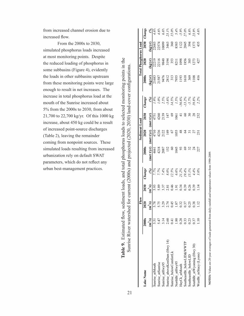
Flow, Sediment, and Phosphorus Delivered to Selected Monitoring Points
In all cases in this “what-when” scenario of projected land-use change, infiltration was reduced and runoff increased. Increases in URHD and URLD lands are accompanied by increases in impervious surfaces relative to the previous land cover. Conversion of agricultural land, forest, or grassland to rural residential is accompanied by assumed compaction and increase in impervious cover. For technical readers, the model simulates these changes by increasing the effective “curve number” of these landscape units. With higher curve numbers, more water runs off directly rather than infiltrating, which in turn reduces the loss of soil water to evapotranspiration, and this reduced loss translates into increased flow. Hence, for the watershed as a whole, flow would increase by about 8% from the 2000s to 2030 given the projected increase in urban and rural residential lands (Table 9). Flow may change by a greater or lesser amount at upstream monitoring sites, but in each case flow increases. Urban best management practices could probably ameliorate some of these projected increases.
Loads of sediment and nutrients at selected monitoring points along the river incorporate all possible sources, including delivery from each upstream subbasin, from each upstream lake, from channel erosion, from groundwater discharge, and from point sources. At the outlet of the watershed, sediment load would increase by about 2%, and total phosphorus load would increase by about 5% from the 2000s to 2030 (Table 9). The increase in sediment appeared to come partly from high-density urbanization along the I-35 corridor and adjacent cities and partly
21
from increased channel erosion due to increased flow.
From the 2000s to 2030, simulated phosphorus loads increased at most monitoring points. Despite the reduced loading of phosphorus in some subbasins (Figure 4), evidently the loads in other subbasins upstream from these monitoring points were large enough to result in net increases. The increase in total phosphorus load at the mouth of the Sunrise increased about 5% from the 2000s to 2030, from about 21,700 to 22,700 kg/yr. Of this 1000 kg increase, about 450 kg could be a result of increased point-source discharges (Table 2), leaving the remainder coming from nonpoint sources. These simulated loads resulting from increased urbanization rely on default SWAT parameters, which do not reflect any urban best-management practices.
Lake
Nam
e20
00s
2020
2030
Chan
ge20
00s
2020
2030
Chan
ge20
00s
2020
2030
Chan
ge(m
3 /s)
(m3 /s
)(m
3 /s)
(%)
(met
t/yr
)(m
et t/
yr)
(met
t/yr
)(%
)(k
g/yr
)(k
g/yr
)(k
g/yr
)(%
)Su
nris
e_at
Mou
th5.
515.
785.
937.7%
4661
4710
4751
1.9%
2168
322
219
2268
34.6%
Sunr
ise_
atSu
nris
e5.
475.
755.
897.7%
4218
4236
4260
1.0%
2158
722
116
2257
44.6%
Sunr
ise_
atH
wy9
53.
143.
293.
377.4%
2087
2122
2139
2.5%
9476
9840
1009
96.6%
Sunr
ise_
abov
eKos
tDam
(Hw
y 14
)2.
602.
742.
818.0%
152
149
147
-3.6%
2812
3194
3463
23.1%
Sunr
ise_
belo
wC
omfo
rtLk
0.41
0.45
0.46
12.5%
6067
6914
.5%
313
353
360
15.0%
Nor
thB
r_at
Hw
y95
1.80
1.87
1.91
6.6%
1045
1055
1061
1.5%
7955
8211
8383
5.4%
Hay
Ck_
atM
outh
0.28
0.32
0.34
21.2%
9348
41-56.6%
1193
1098
1122
-5.9%
Sout
heas
tBr_
belo
wLI
D&
WW
TP0.
330.
370.
3919
.4%
6964
60-13.2%
1610
1856
2045
27.0%
Sout
heas
tBr_
belo
wLI
D0.
230.
250.
2615
.1%
3231
30-5.7%
369
385
394
6.8%
Sout
hBr_
atW
yom
ing
(Hw
y 30
)0.
370.
380.
394.4%
2427
2819
.8%
1108
1273
1373
23.9%
Wes
tBr_
nrSt
acy
(Lyo
ns)
1.10
1.12
1.14
3.0%
227
231
232
2.2%
416
427
435
4.6%
Sedi
men
t Loa
dTo
tal P
hosp
horu
s Loa
dFl
ow
NO
TES:
Val
ues a
re 2
0-ye
ar a
vera
ges o
f loa
ds g
ener
ated
from
dai
ly ra
infa
ll an
d te
mpe
ratu
re v
alue
s fro
m 1
990-
2009
.
Tabl
e 9.
Est
imat
ed fl
ow, s
edim
ent l
oads
, and
tota
l pho
spho
rus l
oads
to se
lect
ed m
onito
ring
poin
ts in
the
Sunr
ise
Riv
er w
ater
shed
for c
urre
nt (2
000s
) and
pro
ject
ed (2
020,
203
0) la
nd-c
over
con
figur
atio
ns.
22
Scenario Set 2: Changes in Agricultural Practices
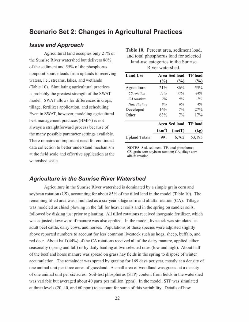
Issue and ApproachAgricultural land occupies only 21% of
the Sunrise River watershed but delivers 86% of the sediment and 55% of the phosphorus nonpoint-source loads from uplands to receiving waters, i.e., streams, lakes, and wetlands (Table 10). Simulating agricultural practices is probably the greatest strength of the SWAT model. SWAT allows for differences in crops, tillage, fertilizer application, and scheduling. Even in SWAT, however, modeling agricultural best management practices (BMPs) is not always a straightforward process because of the many possible parameter settings available. There remains an important need for continued data collection to better understand mechanism at the field scale and effective application at the watershed scale.
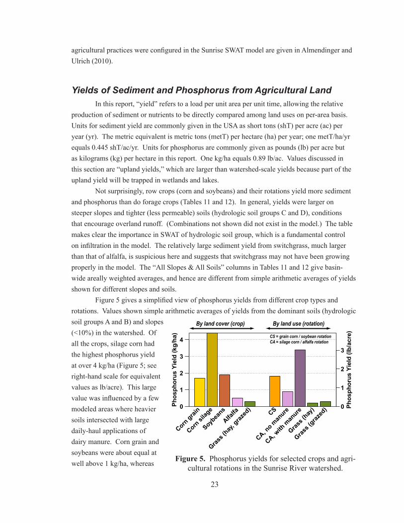
Agriculture in the Sunrise River WatershedAgriculture in the Sunrise River watershed is dominated by a simple grain corn and
soybean rotation (CS), accounting for about 85% of the tilled land in the model (Table 10). The remaining tilled area was simulated as a six-year silage corn and alfalfa rotation (CA). Tillage was modeled as chisel plowing in the fall for heavier soils and in the spring on sandier soils, followed by disking just prior to planting. All tilled rotations received inorganic fertilizer, which was adjusted downward if manure was also applied. In the model, livestock was simulated as adult beef cattle, dairy cows, and horses. Populations of these species were adjusted slightly above reported numbers to account for less common livestock such as hogs, sheep, buffalo, and red deer. About half (44%) of the CA rotations received all of the dairy manure, applied either seasonally (spring and fall) or by daily hauling at two selected rates (low and high). About half of the beef and horse manure was spread on grass hay fields in the spring to dispose of winter accumulation. The remainder was spread by grazing for 169 days per year, mostly at a density of one animal unit per three acres of grassland. A small area of woodland was grazed at a density of one animal unit per six acres. Soil-test phosphorus (STP) content from fields in the watershed was variable but averaged about 40 parts per million (ppm). In the model, STP was simulated at three levels (20, 40, and 60 ppm) to account for some of this variability. Details of how
Land Use Area Sed load TP load(%) (%) (%)
Agriculture 21% 86% 55%CS rotation 11% 77% 44%CA rotation 2% 9% 7%Hay, Pasture 8% 0% 4%
Developed 16% 7% 27%Other 63% 7% 17%
Area Sed load TP load(km2) (metT) (kg)
Upland Totals 991 6,762 53,195
NOTES: Sed, sediment; TP, total phosphorus; CS, grain corn-soybean rotation; CA, silage corn-alfalfa rotation.
Table 10. Percent area, sediment load, and total phosphorus load for selected
land-use categories in the Sunrise River watershed.
23
agricultural practices were configured in the Sunrise SWAT model are given in Almendinger and Ulrich (2010).
Yields of Sediment and Phosphorus from Agricultural LandIn this report, “yield” refers to a load per unit area per unit time, allowing the relative
production of sediment or nutrients to be directly compared among land uses on per-area basis. Units for sediment yield are commonly given in the USA as short tons (shT) per acre (ac) per year (yr). The metric equivalent is metric tons (metT) per hectare (ha) per year; one metT/ha/yr equals 0.445 shT/ac/yr. Units for phosphorus are commonly given as pounds (lb) per acre but as kilograms (kg) per hectare in this report. One kg/ha equals 0.89 lb/ac. Values discussed in this section are “upland yields,” which are larger than watershed-scale yields because part of the upland yield will be trapped in wetlands and lakes.
Not surprisingly, row crops (corn and soybeans) and their rotations yield more sediment and phosphorus than do forage crops (Tables 11 and 12). In general, yields were larger on steeper slopes and tighter (less permeable) soils (hydrologic soil groups C and D), conditions that encourage overland runoff. (Combinations not shown did not exist in the model.) The table makes clear the importance in SWAT of hydrologic soil group, which is a fundamental control on infiltration in the model. The relatively large sediment yield from switchgrass, much larger than that of alfalfa, is suspicious here and suggests that switchgrass may not have been growing properly in the model. The “All Slopes & All Soils” columns in Tables 11 and 12 give basin-wide areally weighted averages, and hence are different from simple arithmetic averages of yields shown for different slopes and soils.
Figure 5 gives a simplified view of phosphorus yields from different crop types and rotations. Values shown simple arithmetic averages of yields from the dominant soils (hydrologic soil groups A and B) and slopes (<10%) in the watershed. Of all the crops, silage corn had the highest phosphorus yield at over 4 kg/ha (Figure 5; see right-hand scale for equivalent values as lb/acre). This large value was influenced by a few modeled areas where heavier soils intersected with large daily-haul applications of dairy manure. Corn grain and soybeans were about equal at well above 1 kg/ha, whereas
0
1
2
3
4
Corn grai
n
Corn si
lage
Soybea
ns
Alfalfa
Grass (
hay, g
razed
)CS
CA, no m
anure
CA, with
man
ure
Grass (
hay)
Grass (
grazed
)
Phos
phor
us Y
ield
(kg/
ha)
0
1
2
3Ph
osph
orus
Yie
ld (l
b/ac
re)
By land cover (crop) By land use (rotation)
CS = grain corn / soybean rotationCA = silage corn / alfalfa rotation
figure 5. Phosphorus yields for selected crops and agri-cultural rotations in the Sunrise River watershed.
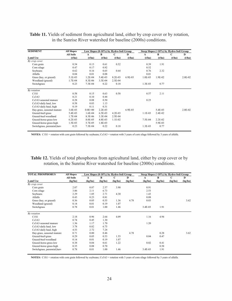
24
SEDIMENT All SlopesAll Soils A B C D A B C D
Land Use (t/ha) (t/ha) (t/ha) (t/ha) (t/ha) (t/ha) (t/ha) (t/ha) (t/ha)By crop cover
Corn grain 0.54 0.13 0.61 0.52 0.39 1.91Corn silage 0.47 0.17 0.92 0.52Soybeans 0.62 0.16 0.65 0.64 0.76 2.32Alfalfa 0.04 0.01 0.08 0.01Grass (hay, or grazed) 5.1E-03 1.2E-04 5.4E-03 8.2E-03 6.9E-03 1.0E-03 1.9E-02 2.0E-02Woodland (grazed) 1.7E-04 8.3E-06 3.3E-04 2.5E-04Switchgrass 0.23 7.3E-04 0.22 0.18 1.3E-03 0.77
By rotationC1S1 0.58 0.15 0.63 0.58 0.57 2.11Cs3A3 0.21 0.10 0.44Cs3A3-seasonal manure 0.28 0.08 0.50 0.25Cs3A3-daily haul, low 0.58 0.03 1.13Cs3A3-daily haul, high 0.19 0.11 0.31Hay-grass, seasonal manure 3.6E-03 0.0E+00 2.2E-03 6.9E-03 5.4E-03 2.0E-02Grazed-beef-grass 5.4E-03 1.6E-04 6.5E-03 4.2E-03 1.1E-03 2.4E-02Grazed-beef-woodland 1.7E-04 8.3E-06 3.3E-04 2.5E-04Grazed-horse-grass-low 6.2E-03 8.0E-05 4.8E-03 1.1E-02 7.5E-04 2.2E-02Grazed-horse-grass-high 1.5E-03 5.7E-05 1.8E-03 5.9E-03Switchgrass, perennial,harv 0.23 7.3E-04 0.22 0.18 1.3E-03 0.77
Low Slopes (0-10%) by Hydro-Soil Group Steep Slopes (>10%) by Hydro-Soil Group
NOTES: C1S1 = rotation with corn grain followed by soybeans; Cs3A3 = rotation with 3 years of corn silage followed by 3 years of alfalfa.
Table 11. Yields of sediment from agricultural land, either by crop cover or by rotation, in the Sunrise River watershed for baseline (2000s) conditions.
Table 12. Yields of total phosphorus from agricultural land, either by crop cover or by rotation, in the Sunrise River watershed for baseline (2000s) conditions.
TOTAL PHOSPHORUS All SlopesAll Soils A B C D A B C D
Land Use (kg/ha) (kg/ha) (kg/ha) (kg/ha) (kg/ha) (kg/ha) (kg/ha) (kg/ha) (kg/ha)By crop cover
Corn grain 2.07 0.87 2.57 3.90 0.91Corn silage 3.86 2.11 6.73 2.53Soybeans 2.29 1.05 2.71 4.30 1.43Alfalfa 0.43 0.23 0.81 0.08Grass (hay, or grazed) 0.36 0.05 0.55 1.36 4.78 0.03 3.62Woodland (grazed) 0.14 0.01 0.19 1.07Switchgrass 0.78 0.01 1.00 1.46 3.4E-03 1.91
By rotationC1S1 2.18 0.96 2.64 4.09 1.16 4.94Cs3A3 0.74 0.45 1.30Cs3A3-seasonal manure 1.36 1.17 1.70 1.20Cs3A3-daily haul, low 3.78 0.82 6.75Cs3A3-daily haul, high 4.53 2.72 7.24Hay-grass, seasonal manure 0.71 0.00 0.46 4.78 0.28 3.62Grazed-beef-grass 0.29 0.05 0.53 1.55 0.04 0.47Grazed-beef-woodland 0.14 0.01 0.19 1.07Grazed-horse-grass-low 0.38 0.04 0.61 1.22 0.02 0.41Grazed-horse-grass-high 0.35 0.08 0.70 0.58Switchgrass, perennial,harv 0.78 0.01 1.00 1.46 3.4E-03 1.91
Low Slopes (0-10%) by Hydro-Soil Group Steep Slopes (>10%) by Hydro-Soil Group
NOTES: C1S1 = rotation with corn grain followed by soybeans; Cs3A3 = rotation with 3 years of corn silage followed by 3 years of alfalfa.
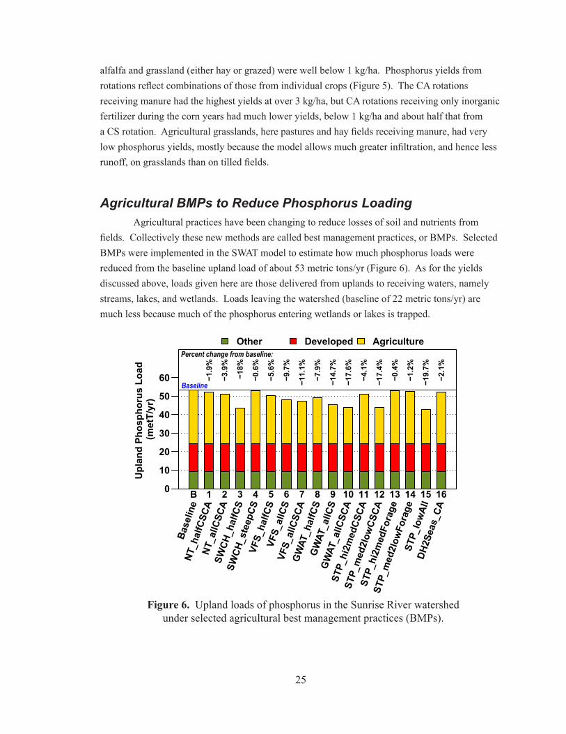
25
alfalfa and grassland (either hay or grazed) were well below 1 kg/ha. Phosphorus yields from rotations reflect combinations of those from individual crops (Figure 5). The CA rotations receiving manure had the highest yields at over 3 kg/ha, but CA rotations receiving only inorganic fertilizer during the corn years had much lower yields, below 1 kg/ha and about half that from a CS rotation. Agricultural grasslands, here pastures and hay fields receiving manure, had very low phosphorus yields, mostly because the model allows much greater infiltration, and hence less runoff, on grasslands than on tilled fields.
Agricultural BMPs to Reduce Phosphorus LoadingAgricultural practices have been changing to reduce losses of soil and nutrients from
fields. Collectively these new methods are called best management practices, or BMPs. Selected BMPs were implemented in the SWAT model to estimate how much phosphorus loads were reduced from the baseline upland load of about 53 metric tons/yr (Figure 6). As for the yields discussed above, loads given here are those delivered from uplands to receiving waters, namely streams, lakes, and wetlands. Loads leaving the watershed (baseline of 22 metric tons/yr) are much less because much of the phosphorus entering wetlands or lakes is trapped.
0
10
20
30
40
50
60
Upl
and
Phos
phor
us L
oad
(met
T/yr
)
B 1 2 3 4 5 6 7 8 9 10 11 12 13 14 15 16
Base
line
NT_h
alfC
SCA
NT_a
llCSC
ASW
CH_h
alfC
SSW
CH_s
teep
CSVF
S_ha
lfCS
VFS_
allC
SVF
S_al
lCSC
AG
WAT
_hal
fCS
GW
AT_a
llCS
GW
AT_a
llCSC
AST
P_hi
2med
CSCA
STP_
med
2low
CSCA
STP_
hi2m
edFo
rage
STP_
med
2low
Fora
geST
P_lo
wAl
lDH
2Sea
s_CA
Other Developed Agriculture
−1.9%
−3.9%
−18%
−0.6%
−5.6%
−9.7%
−11.1%
−7.9%
−14.7%
−17.6%
−4.1%
−17.4%
−0.4%
−1.2%
−19.7%
−2.1%
Percent change from baseline:
Baseline
figure 6. Upland loads of phosphorus in the Sunrise River watershed under selected agricultural best management practices (BMPs).
26
No-till (NT): No-till agriculture tends to reduce sediment loads because of increased vegetative and
residue cover that protects the soil from erosion. However, the effect of no-till agriculture on phosphorus loads is not so straightforward. Because of reduced sediment loss, no-till agriculture also tends to reduce loss of sediment-bound phosphorus; however, because of the increased plant-derived surface residue, the loss of soluble phosphorus may increase. In the Sunrise SWAT model, if only tillage operations were removed and surface roughness increased, then sediment loads decreased but phosphorus loads increased. If in addition infiltration rates and biological mixing of residue were increased, then phosphorus loads were slightly reduced. We chose the latter configuration in hopes that it was broadly representative but recognize that the results may be variable in the real world. For the technical reader, no-till agriculture was modeled by removing tillage operations, increasing overland N from 0.14 to 0.3, reducing curve numbers by 5%, and increasing bio-mixing efficiency from 0.2 to 0.5.
The results were decidedly modest in terms of phosphorus reductions (Figure 6). Scenarios 1 and 2 converted half, and then all, of the CS and CA rotations to no-till agriculture, and reductions in upland phosphorus load were only about 2% and 4%, respectively. We note that these results depended on somewhat arbitrary increases in infiltration rate and bio-mixing, and that more data are needed to know how to set these parameters. Nonetheless, no-till practices seem more effective at reducing losses of sediment than phosphorus.
Switchgrass (SWCH): Switchgrass is a potential crop for energy production from biomass. Alamo switchgrass
is available in SWAT’s crop data base, although other varieties are likely better suited for growing in the upper Midwest. In the Sunrise SWAT model, switchgrass was implemented by setting it as the perennial cover in a selected land unit (HRU), adding 400 kg of 28-03-00 fertilizer on 1 May (about 100 lb/ac N and 5 lb/ac P), and harvesting on 1 November. Eighty-percent of the biomass was considered yield (HI_OVR = 0.8), and all of the yield was removed (HARVEFF = 1) each year.
Scenario 3 (Figure 6) converted half the CS lands to perennial switchgrass, and phosphorus loads were substantially reduced by 18%. Scenario 4 replaced all CS lands on steep slopes with switchgrass, which is good management, but there were so few of these areas in the model that the result was inconsequential.
Similar scenarios were run with smooth brome and a generic prairie-grass type parameterized to better simulate a community of different grass species, with a longer effective growing season than a monospecific stand of grass (Dr. Brent Dalzell, Univ. of Minnesota, personal communication). Results were similar to those for switchgrass. However, we note that the biomass of these grasses in the model seemed much too small (e.g., about 1 metT/ha for switchgrass) when implemented as perennial vegetation, which may be an idiosyncrasy of SWAT.
27
A different implementation of grassland, with annual planting, may produce different results with greater biomass.
Vegetated filter strips (VFS): A VFS is a strip of grassland along the downhill edge of an HRU, here set to 2% of the
HRU area. For an HRU representing a square 40-acre field, the strip would be about 25 ft wide (8 meters). The VFS was assumed to treat 25% of runoff from the HRU, or a 100-m-wide strip immediately upgradient from the VFS in our example 40-acre field. The remaining 75% of the HRU (more than 100 m away) was assumed to form concentrated flow that bypassed the VFS. Note that SWAT’s VFS corresponds to a buffer strip along a waterway only for the idealized case where the field edge is both along the receiving stream and also the lowermost part of an overland-flow plane (i.e., sloping land conveying sheet flow). In the real world, the lower edge of a flow plane may more likely be along an ephemeral flow path or ditch within a field, in which case there is little distinction between a VFS and grassed waterway.
Resulting phosphorus load reductions were substantial (Figure 6). Adding a VFS to half or all CS lands (scenarios 5 and 6) resulted in load reductions of about 6-10%. Adding VFSs to CA lands as well (scenario 7) resulted in little additional reduction, mostly because the area of CA lands was small.
Grassed waterways (GWAT): Grassed waterways (GWATs) in SWAT have the benefits of vegetated filter strips (VFSs)
that trap sediment and nutrients from sheet flow passing transversely through the strip, plus the additional benefit of trapping constituents from water flowing longitudinally along the waterway. In the Sunrise SWAT model, GWATs were implemented as a 10-m wide strip of grassland with a length set to the square root of the field area, e.g., a single waterway down the middle of a square field. For a 40-acre field, this would amount to about 2.5% of the total field area. All other parameters (channel roughness and particle transport parameters) were left at default values.
Results were consistent with the VFS results, namely that GWATs provided substantial reductions in phosphorus loads (Figure 6). Scenarios 8-10 implemented GWATs on half of CS land, all of CS land, and all of both CS and CA lands, respectively, and resulted in reductions in phosphorus loads of 8-18%.
Soil-test phosphorus (STP) reductions: STP can be lowered by reducing fertilizer additions of phosphorus below that removed
by crop harvest and runoff. Reductions in STP of a few parts per million (ppm) per year could require several decades to reach target levels. In theory SWAT should be able to track the reduction in STP over time, but this ability has not yet been well tested.
28
Scenario 11 (Figure 6) reduced STP in the CS and CA lands with high STP (60 ppm) down to medium levels (40 ppm). The reduction in load (4%) was modest but useful because implementation required only 25% of the tilled lands, those with the highest STP. Scenario 12 reduced STP to 20 ppm in all CS land and 30 ppm in all CA land, thereby reducing phosphorus loads by a substantial 17%. Scenarios 13 and 14 reduced STP in grass hay fields and pasture (forage crops), first in those few grasslands with high (60 ppm) levels down to medium (40 ppm), and second in all grasslands down to 20 ppm. Load reductions were modest because such grasslands were not large contributors of phosphorus in the first place in the model. However, combining all these STP reductions (scenario 15) resulted in a nearly 20% reduction in phosphorus load.
Converting daily-haul (DH) manure applications to seasonal: Seasonal applications of manure, if incorporated by chisel plowing, can reduce
phosphorus loads compared to daily-haul operations that spread some manure on frozen ground in early spring. Converting all daily haul operations on CA land to seasonal manure applications (scenario 16, Figure 6) resulted in only a modest phosphorus load reduction (2%), mostly because of the small area of these lands.
ConclusionsEven though the phosphorus load reduction from any one agricultural BMP may be
modest, in aggregate the reductions could be substantial. Furthermore, the model could not include the entire range of large STP values or manure application rates that might be present in the watershed. Resource managers should expect to find such sites and to target them first for remediation.
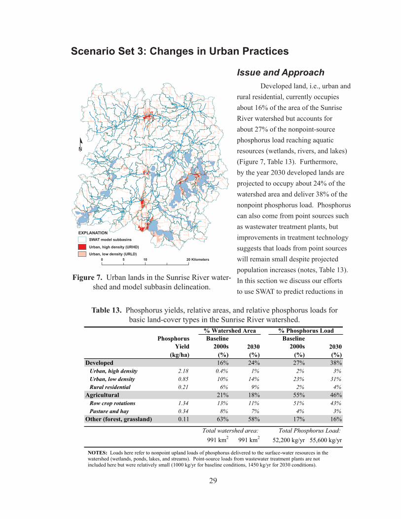
29
Scenario Set 3: Changes in Urban Practices
Issue and ApproachDeveloped land, i.e., urban and
rural residential, currently occupies about 16% of the area of the Sunrise River watershed but accounts for about 27% of the nonpoint-source phosphorus load reaching aquatic resources (wetlands, rivers, and lakes) (Figure 7, Table 13). Furthermore, by the year 2030 developed lands are projected to occupy about 24% of the watershed area and deliver 38% of the nonpoint phosphorus load. Phosphorus can also come from point sources such as wastewater treatment plants, but improvements in treatment technology suggests that loads from point sources will remain small despite projected population increases (notes, Table 13). In this section we discuss our efforts to use SWAT to predict reductions in
0 10 205 Kilometers
EXPLANATIONSWAT model subbasins
Urban, high density (URHD)
Urban, low density (URLD)
figure 7. Urban lands in the Sunrise River water-shed and model subbasin delineation.
PhosphorusYield
Baseline2000s 2030
Baseline2000s 2030
(kg/ha) (%) (%) (%) (%)Developed 16% 24% 27% 38%
Urban, high density 2.18 0.4% 1% 2% 3%Urban, low density 0.85 10% 14% 23% 31%Rural residential 0.21 6% 9% 2% 4%
Agricultural 21% 18% 55% 46%Row crop rotations 1.34 13% 11% 51% 43%Pasture and hay 0.34 8% 7% 4% 3%
Other (forest, grassland) 0.11 63% 58% 17% 16%
Total watershed area: Total Phosphorus Load:991 km2 991 km2 52,200 kg/yr 55,600 kg/yr
% Watershed Area % Phosphorus Load
NOTES: Loads here refer to nonpoint upland loads of phosphorus delivered to the surface-water resources in the watershed (wetlands, ponds, lakes, and streams). Point-source loads from wastewater treatment plants are not included here but were relatively small (1000 kg/yr for baseline conditions, 1450 kg/yr for 2030 conditions).
Table 13. Phosphorus yields, relative areas, and relative phosphorus loads for basic land-cover types in the Sunrise River watershed.
30
nonpoint phosphorus loads from developed lands by changing selected characteristics of these lands in the model. Loads of sediment from urban areas can be substantial and should not be ignored in many cases. However, in the Sunrise watershed urban sources of sediment appear small compared to agricultural sources (see Table 10) and channel erosion (about 46% of total sediment leaving the watershed).
SWAT Model Hydrology and Developed LandsTo understand the how SWAT could simulate reductions in phosphorus load, a review of
SWAT’s conceptualization of watershed hydrology is useful. The SWAT model subdivided the Sunrise watershed into 142 subbasins (Figure 7), each of which was composed of many land use and soil combinations that represent uplands; each land-use, soil, and slope combination is called a hydrologic response unit, or HRU. On a daily time step, the model routes some stormflow, snowmelt, and groundwater flow from the uplands to wetlands (if present in a subbasin), which remove some phosphorus before delivering outflow to streams and lakes. The remainder of water from each HRU enters the streams and lakes directly. On days with no storm or snowmelt runoff (i.e., most days), stream flow is maintained by groundwater discharge.
Three types of developed uplands were modeled: high-density urban (URHD), low-density urban (URLD), and rural residential (RRES). URHD corresponds to commercial properties and apartment-style residences. URLD corresponds to single-family homes in villages and lakeshores, about two homes per three acres, and also to the roadway network in the watershed, which adds considerable area to the URLD land-use type beyond municipal boundaries. RRES lands were modeled with soil permeabilities and phosphorus contents about mid-way between pristine conditions (grassland and woodland) and URLD lands.
By default, SWAT estimates phosphorus yields (load per unit area) from URHD and URLD based on regression equations developed in the 1980s. URHD lands had the highest phosphorus yield of all land-use types, exceeding even that of row-crop agriculture (Table 13). URLD lands had phosphorus yields within the range of agricultural lands. RRES lands had lower phosphorus yields than agricultural land but still about twice that of undeveloped land (forest and grassland).
Modeled Scenarios to Reduce Phosphorus Loads from Developed Lands
Phosphorus loads from uplands can be reduced in either of two ways. First, the amount of surface (overland) runoff that transports the phosphorus can be reduced. Second, the phosphorus content of that runoff can be reduced. Modeled upland phosphorus loads from scenarios attempting to use these methods were compared to current baseline (2000-10) loads, as well as to projected loads for the year 2030 (Figure 8). Note that the watershed-wide total
31
phosphorus load from the uplands exceeds 50 metric tons per year (bars, Figure 8), which is far greater than the total load delivered from the Sunrise to the St. Croix River (cross-hair symbols, Figure 8). The difference is caused by the trapping of phosphorus in lowlands (ponds, wetlands) and lakes. These water bodies help protect the St. Croix River from excess phosphorus but can suffer from impaired water quality themselves as a consequence.
Baseline and 2030 Projection Model Runs (Figure 8, scenarios B and 1) Baseline upland phosphorus loads totaled about 52.2
met T (metric tons; 1 met T = 2,200 pounds, or 1.1 short tons), about 27% of which comes from developed lands (Table 13). Expansion of existing urban and rural residential areas to accommodate projected population increases by 2030 may increase the upland phosphorus load by 6%, to 55.6 met T. This increase assumes conventional urban development as characterized by the 1980s regression equations.
0
10
20
30
40
50
60
70
Pho
spho
rus
Load
(m
etT/
yr)
B 1 2 3 4 5 6 7 8
Base
line
2030
Pro
ject
ion
URHD
_FIM
P-20
%UR
HD_F
CIM
P-20
%UR
LD_F
IMP-
20%
URLD
_FCI
MP-
20%
IMP_
CN-1
0%RR
ES_C
N na
tura
lRR
ES_S
TP-1
0ppm
Load from uplands to water resources:Other Agricultural Developed
0% 6% 0% 0% 0% -3%
-1%
-1%
-1%
Baseline
Change from baseline:
Load from Sunriseto St. Croix:
figure 8. Upland phosphorus loads for basic land-cover types under selected scenarios to reduce loads from developed lands (URHD, URLD, and RRES).
URHD = urban high-density, URLD = urban low-density, RRES = rural residential, FIMP = fraction im-pervious, FCIMP = fraction connected impervious, IMP = impervious, CN = curve number, STP = soil-test
phosphorus.
32
Scenarios to Reduce Runoff (Figures 8 and 9, scenarios 2-7) Runoff from urban lands can be greatly influenced
by the fraction of impervious cover (FIMP) and connected impervious cover (FCIMP), which are directly connected to channelized flow paths provided by curbs, gutters, and storm sewers. SWAT defaults to FIMP and FCIMP values of 0.6 and 0.44 for URHD, and 0.12 and 0.10 for URLD lands. For each scenario, Figure 9 shows total runoff volume from developed lands as well as from other (forest and grassland) and agricultural lands for perspective. Note that of the developed lands, most runoff is generated by URLD lands (Figure 9, pink) because of their larger area than URHD lands (Table 13) and lower infiltration capacity than RRES lands.
Scenarios 2-5 tested the effect of reducing FIMP and FCIMP by 20% in URHD and URLD lands, respectively. Runoff was in fact reduced, but only slightly, about 1% or less for scenarios 2-4 and 5% for scenario 5 (Figure 9). Consequently, modeled reductions in upland phosphorus loads were insubstantial, essentially zero for scenarios 2-4 and only 3% for scenario 5 (Figure 8). Reduction in impervious cover of 20% is a fairly dramatic change, and equations in the SWAT theory manual (Neitsch et al. 2011) suggest that phosphorus loads from URHD and URLD should have been likewise reduced by about 20% from those land covers. Since the URHD and URLD types were responsible for about 25% of the total upland phosphorus load
0
500
1000
1500
2000
2500
3000Su
rfac
e R
unof
f Vol
ume
(ha−
m/y
r)
B 1 2 3 4 5 6 7
Base
line
2030
Pro
ject
ion
URHD
_FIM
P−20
%UR
HD_F
CIM
P−20
%UR
LD_F
IMP−
20%
URLD
_FCI
MP−
20%
IMP_
CN−1
0%RR
ES_C
N na
tura
l
EXPLANATIONOtherAgricultural
Rural Residential (RRES)Urban, Low−Density (URLD)Urban, High−Density (URHD)
0% 16%
−1%
−1% 0% −5%
−2%
−1%
Baseline
Change from baseline:
figure 9. Surface runoff volumes for selected land-cover categories in the Sun-rise River watershed for developed land-cover scenarios.
One ha-m is the volume of water needed to cover a hectare with 1 m of water. URHD = urban high-density, URLD = urban low-density, RRES = rural residential, FIMP = fraction impervious, FCIMP = fraction con-
nected impervious, IMP = impervious, CN = curve number.
33
under baseline conditions (Table 13), the upland load should have been reduced by about one-fifth, or 5%. Scenario 6 tested the effect of changing totally impervious surfaces to having some infiltration capacity, for example by having pervious pavement. (Technically, this was done by reducing the curve number (CN) of impervious surfaces by 10%, from 98 to 88.) Again, reductions in runoff volume (2%, Figure 9) and upland phosphorus load (1%, Figure 8) were insubstantial. The minimal changes seen in our model runs suggest that there are idiosyncrasies in the SWAT code dealing with URHD and URLD lands that need further examination.
Scenario 7 modeled the effect of increasing the infiltration capacity of RRES lands to the natural state of grasslands or woodlands. However, runoff was not large from RRES lands in the baseline model (Figure 9, orange segment), and so reducing runoff further resulted in only minor reductions in the total volume of runoff and in upland phosphorus loads (Figure 8).
Scenario to Reduce Phosphorus Content of Runoff(Figure 8, scenario 8) The phosphorus content of runoff can be reduced by reducing
the phosphorus content of the surface soil in contact with the runoff. Scenario 8 tested the effect of reducing the soil-test phosphorus (STP) levels in RRES soils by half, from 20 ppm (part per million) to 10 ppm. Again, because RRES lands delivered a fairly small load in the baseline run, reducing the load further resulted in only a 1% drop in the total upland phosphorus load (Figure 8, scenario 8).
Phosphorus Loading to Lakes and Treatment of Urban Runoff by Wetlands or Ponds
Lakes are among the most highly valued aquatic resources in the Sunrise River watershed, thereby attracting the very development that can contribute to their impairment. Figure 10 shows phosphorus loads to ten selected lakes in the Sunrise River watershed for all the scenarios discussed above, with similarly disappointingly small load reductions.
An alternative to reducing the runoff and phosphorus loads generated by upland urban surfaces is to treat the runoff by routing it through a wetland before discharging it to receiving waters. Scenario 9 (Figure 10) tested the effect of routing an additional 20% of runoff through wetlands for each of the nine subbasins in the model that contained URHD lands, i.e., the most densely urban subbasins. Loads from each of these urban subbasins were reduced substantially, but the total load received by these ten lakes was reduced by only by 4%, which is somewhat disappointing in face of the projected 18% increase in loads by the year 2030. The larger message is that phosphorus loads to these lakes is controlled by more than simply the nine URHD-containing subbasins. In particular, growth of URLD land in other nearby subbasins is the source of most of the projected increase in phosphorus loads, and these subbasins likewise need mitigation efforts. A more exhaustive look at use of wetlands to treat subbasin runoff is presented in the next section of this report.
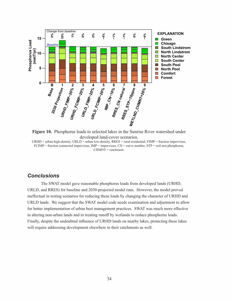
34
ConclusionsThe SWAT model gave reasonable phosphorus loads from developed lands (URHD,
URLD, and RRES) for baseline and 2030-projected model runs. However, the model proved ineffectual in testing scenarios for reducing these loads by changing the character of URHD and URLD lands. We suggest that the SWAT model code needs examination and adjustment to allow for better implementation of urban best management practices. SWAT was much more effective in altering non-urban lands and in treating runoff by wetlands to reduce phosphorus loads. Finally, despite the undoubted influence of URHD lands on nearby lakes, protecting these lakes will require addressing development elsewhere in their catchments as well.
0
5
10
15
Phos
phor
us L
oad
(met
T/yr
)
B 1 2 3 4 5 6 7 8 9
Base
2030
Pro
ject
ion
URHD
_FIMP−
20%
URHD
_FCIMP−
20%
URLD
_FIMP−
20%
URLD
_FCIMP−
20%
IMP_CN
−10%
RRES
_CN
natu
ral
RRES
_STP
−10ppm
WET
LND_
CHMNT
+20%
EXPLANATIONGreenChisagoSouth LindstromNorth LindstromNorth CenterSouth CenterSouth PoolNorth PoolComfortForest
0% 18% 1% 0% 0% −4%
−1%
−1% 0% −4%
Baseline
Change from baseline:
figure 10. Phosphorus loads to selected lakes in the Sunrise River watershed under developed land-cover scenarios.
URHD = urban high-density, URLD = urban low-density, RRES = rural residential, FIMP = fraction impervious, FCIMP = fraction connected impervious, IMP = impervious, CN = curve number, STP = soil-test phosphorus,
CHMNT = catchment.
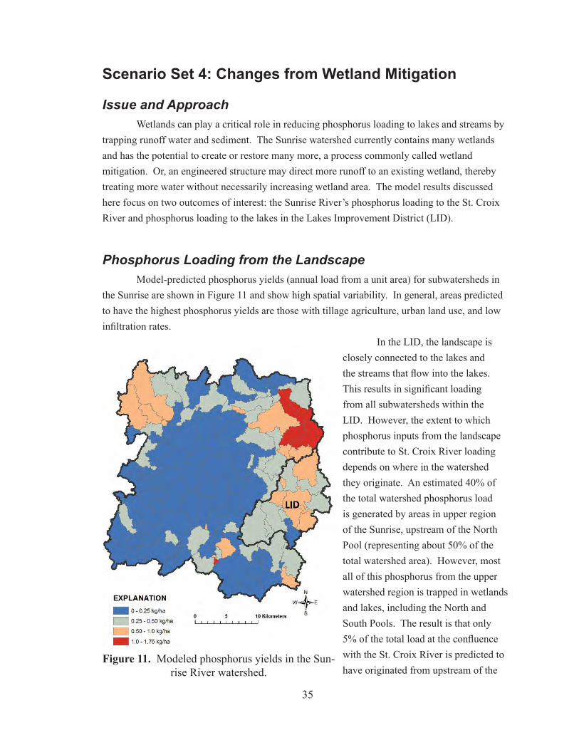
35
Scenario Set 4: Changes from Wetland Mitigation
Issue and ApproachWetlands can play a critical role in reducing phosphorus loading to lakes and streams by
trapping runoff water and sediment. The Sunrise watershed currently contains many wetlands and has the potential to create or restore many more, a process commonly called wetland mitigation. Or, an engineered structure may direct more runoff to an existing wetland, thereby treating more water without necessarily increasing wetland area. The model results discussed here focus on two outcomes of interest: the Sunrise River’s phosphorus loading to the St. Croix River and phosphorus loading to the lakes in the Lakes Improvement District (LID).
Phosphorus Loading from the LandscapeModel-predicted phosphorus yields (annual load from a unit area) for subwatersheds in
the Sunrise are shown in Figure 11 and show high spatial variability. In general, areas predicted to have the highest phosphorus yields are those with tillage agriculture, urban land use, and low infiltration rates.
In the LID, the landscape is closely connected to the lakes and the streams that flow into the lakes. This results in significant loading from all subwatersheds within the LID. However, the extent to which phosphorus inputs from the landscape contribute to St. Croix River loading depends on where in the watershed they originate. An estimated 40% of the total watershed phosphorus load is generated by areas in upper region of the Sunrise, upstream of the North Pool (representing about 50% of the total watershed area). However, most all of this phosphorus from the upper watershed region is trapped in wetlands and lakes, including the North and South Pools. The result is that only 5% of the total load at the confluence with the St. Croix River is predicted to have originated from upstream of the
figure 11. Modeled phosphorus yields in the Sun-
rise River watershed.
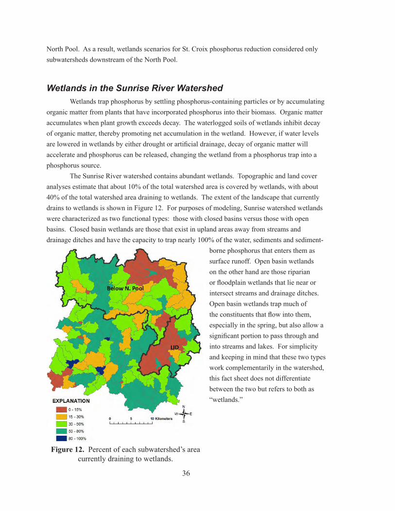
36
North Pool. As a result, wetlands scenarios for St. Croix phosphorus reduction considered only subwatersheds downstream of the North Pool.
Wetlands in the Sunrise River WatershedWetlands trap phosphorus by settling phosphorus-containing particles or by accumulating
organic matter from plants that have incorporated phosphorus into their biomass. Organic matter accumulates when plant growth exceeds decay. The waterlogged soils of wetlands inhibit decay of organic matter, thereby promoting net accumulation in the wetland. However, if water levels are lowered in wetlands by either drought or artificial drainage, decay of organic matter will accelerate and phosphorus can be released, changing the wetland from a phosphorus trap into a phosphorus source.
The Sunrise River watershed contains abundant wetlands. Topographic and land cover analyses estimate that about 10% of the total watershed area is covered by wetlands, with about 40% of the total watershed area draining to wetlands. The extent of the landscape that currently drains to wetlands is shown in Figure 12. For purposes of modeling, Sunrise watershed wetlands were characterized as two functional types: those with closed basins versus those with open basins. Closed basin wetlands are those that exist in upland areas away from streams and drainage ditches and have the capacity to trap nearly 100% of the water, sediments and sediment-
borne phosphorus that enters them as surface runoff. Open basin wetlands on the other hand are those riparian or floodplain wetlands that lie near or intersect streams and drainage ditches. Open basin wetlands trap much of the constituents that flow into them, especially in the spring, but also allow a significant portion to pass through and into streams and lakes. For simplicity and keeping in mind that these two types work complementarily in the watershed, this fact sheet does not differentiate between the two but refers to both as “wetlands.”
figure 12. Percent of each subwatershed’s area
currently draining to wetlands.
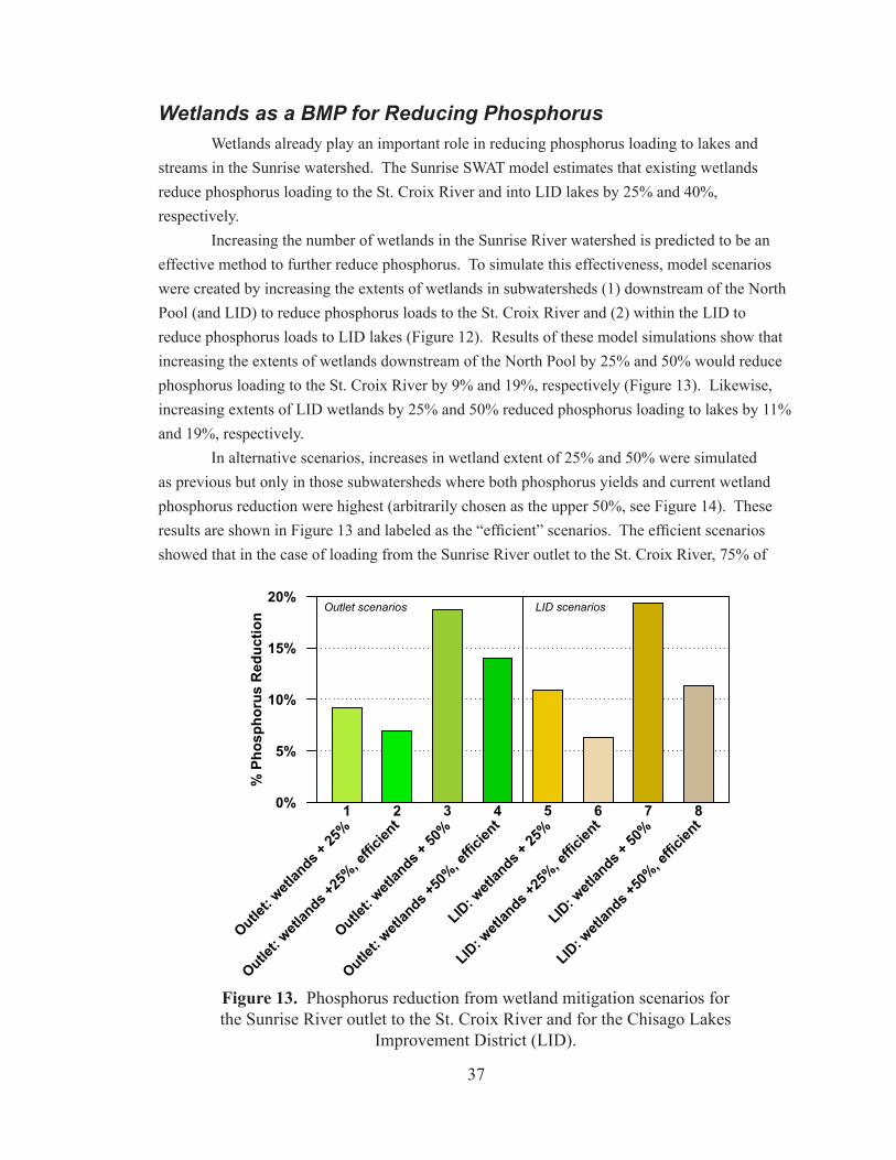
37
Wetlands as a BMP for Reducing PhosphorusWetlands already play an important role in reducing phosphorus loading to lakes and
streams in the Sunrise watershed. The Sunrise SWAT model estimates that existing wetlands reduce phosphorus loading to the St. Croix River and into LID lakes by 25% and 40%, respectively.
Increasing the number of wetlands in the Sunrise River watershed is predicted to be an effective method to further reduce phosphorus. To simulate this effectiveness, model scenarios were created by increasing the extents of wetlands in subwatersheds (1) downstream of the North Pool (and LID) to reduce phosphorus loads to the St. Croix River and (2) within the LID to reduce phosphorus loads to LID lakes (Figure 12). Results of these model simulations show that increasing the extents of wetlands downstream of the North Pool by 25% and 50% would reduce phosphorus loading to the St. Croix River by 9% and 19%, respectively (Figure 13). Likewise, increasing extents of LID wetlands by 25% and 50% reduced phosphorus loading to lakes by 11% and 19%, respectively.
In alternative scenarios, increases in wetland extent of 25% and 50% were simulated as previous but only in those subwatersheds where both phosphorus yields and current wetland phosphorus reduction were highest (arbitrarily chosen as the upper 50%, see Figure 14). These results are shown in Figure 13 and labeled as the “efficient” scenarios. The efficient scenarios showed that in the case of loading from the Sunrise River outlet to the St. Croix River, 75% of
0%
5%
10%
15%
20%
% P
hosp
horu
s R
educ
tion
1 2 3 4 5 6 7 8
Outlet: w
etlan
ds + 25
%
Outlet: w
etlan
ds +25
%, effic
ient
Outlet: w
etlan
ds + 50
%
Outlet: w
etlan
ds +50
%, effic
ient
LID: w
etlan
ds + 25
%
LID: w
etlan
ds +25
%, effic
ient
LID: w
etlan
ds + 50
%
LID: w
etlan
ds +50
%, effic
ient
Outlet scenarios LID scenarios
figure 13. Phosphorus reduction from wetland mitigation scenarios for the Sunrise River outlet to the St. Croix River and for the Chisago Lakes
Improvement District (LID).
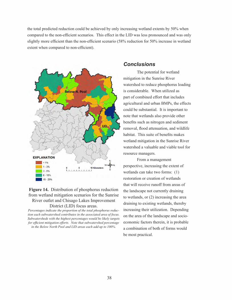
38
the total predicted reduction could be achieved by only increasing wetland extents by 50% when compared to the non-efficient scenarios. This effect in the LID was less pronounced and was only slightly more efficient than the non-efficient scenario (58% reduction for 50% increase in wetland extent when compared to non-efficient).
ConclusionsThe potential for wetland
mitigation in the Sunrise River watershed to reduce phosphorus loading is considerable. When utilized as part of combined effort that includes agricultural and urban BMPs, the effects could be substantial. It is important to note that wetlands also provide other benefits such as nitrogen and sediment removal, flood attenuation, and wildlife habitat. This suite of benefits makes wetland mitigation in the Sunrise River watershed a valuable and viable tool for resource managers.
From a management perspective, increasing the extent of wetlands can take two forms: (1) restoration or creation of wetlands that will receive runoff from areas of the landscape not currently draining to wetlands, or (2) increasing the area draining to existing wetlands, thereby increasing their utilization. Depending on the area of the landscape and socio-economic factors therein, it is probable a combination of both of forms would be most practical.
figure 14. Distribution of phosphorus reduction from wetland mitigation scenarios for the Sunrise
River outlet and Chisago Lakes Improvement District (LID) focus areas.
Percentages indicate the proportion of the total phosphorus reduc-tion each subwatershed contributes in the associated area of focus. Subwatersheds with the highest percentages would be likely targets for efficient mitigation efforts. Note that subwatershed percentage
in the Below North Pool and LID areas each add up to 100%.
39
Summary and ConclusionsWater resources are degraded by loads of sediment and nutrients, much of which arise
from nonpoint sources distributed within the watershed. In particular, too much phosphorus is commonly the single largest cause of eutrophication, where excess algal growth can impair water quality. The Sunrise River watershed has at least four river reaches and ten lakes listed as impaired by the Minnesota Pollution Control Agency. In addition, the Sunrise River is tributary to the St. Croix River, a federally protected waterway also listed as impaired for excess phosphorus in its lowermost 40 km. Reducing phosphorus loads would benefit both the Sunrise and St. Croix watersheds. The largest reductions in phosphorus loads will have to come from nonpoint sources, because they are the largest contributor. To better identify the sources of nonpoint loads, how they are transported to the receiving waters, and how they might be reduced, a computer watershed model of the Sunrise River watershed was constructed with the Soil and Water Assessment Tool (SWAT).
The purpose of this project was to apply the previously constructed SWAT model (revised in autumn of 2011) to selected scenarios in the Sunrise River watershed and quantify the resulting phosphorus loads. Sediment loads were commonly quantified as well. Four sets of scenarios were modeled: (1) changes from projected population growth, (2) changes in agricultural practices, (3) changes in urban practices, and (4) changes from wetland mitigation.
Changes from projected population growth: By the year 2030, population in the Sunrise watershed could increase from 66,000 to 120,000, causing an increase in developed lands from 16% (current) to 24% of the total watershed area. Developed lands here include high- and low-density urban land and rural residential land. Phosphorus loads to rivers and lakes in the watershed would increase by 7%s, and the phosphorus load from the Sunrise to the St. Croix would increase by 5%. Lakes nearest expanding urban centers would receive the largest phosphorus increases, commonly exceeding 10%. Mitigation of urban runoff would greatly benefit these lakes.
Changes in agricultural practices: The most effective best management practices (BMPs) were those that reduced phosphorus content in runoff by reducing soil-test phosphorus levels (up to 20% reduction in loads) and those that treated runoff in grassed waterways (18% reduction) or vegetated filter strips (11% reduction). These reductions assume full implementation on every corn, soybean, and alfalfa field, which is unlikely, but partial implementation could still result in substantial load reductions. No-till scenarios were much more effective at reducing sediment loads than phosphorus.
Changes in urban practices: The SWAT model gave reasonable phosphorus loads from developed lands for baseline and projected-population model runs. However, the model proved ineffectual in testing scenarios for reducing these loads by changing the character of urban lands. According to the literature (including the SWAT theoretical manual), reductions in fraction of impervious area should decrease phosphorus loads substantially, yet phosphorus loads in the Sunrise model were insensitive to such changes. We suggest that the SWAT model code
40
needs examination and adjustment to allow for better implementation of urban best management practices. SWAT was much more effective in altering non-urban lands and in treating runoff by wetlands to reduce phosphorus loads. Finally, despite the undoubted influence of high-density urban lands on nearby lakes, protecting these lakes will require addressing other development (low-density urban and rural residential) elsewhere in their catchments as well.
Changes from wetland mitigation: Calibration of the Sunrise SWAT model indicated that a substantial fraction of runoff in the watershed is already treated by passing through wetlands. Increasing the catchment area of these wetlands, or restoring additional wetland basins, could substantially reduce phosphorus loads reaching streams and lakes. Depending on available sites, reductions of about 6 to 19% could be achieved in the Chisago Lake Improvement District, and about 7 to 18% could be achieved at the watershed outlet. Because most phosphorus generated in the upper watershed (above the North Pool) is already trapped by wetlands and lakes, wetland mitigation there would have little effect in reducing loads from the Sunrise to the St. Croix, though it presumably would benefit local water resources.
Overall we conclude that reducing nonpoint load of phosphorus is feasible, but that there is no easy solution. Reducing loads from the agricultural sector would require substantial participation in land management (e.g., grassed waterways) and reduced phosphorus applications. Treating runoff with wetland mitigation would require substantial wetland creation or re-routing of runoff through existing wetlands. Reducing urban runoff should substantially benefit the adjacent lakes, although we were unable to effectively simulate urban BMPs in SWAT. Implementing urban BMPs will be particularly important in the face of projected increases in population and development pressure. Even if these changes do not occur by the year 2030, we presume they will occur eventually.
AcknowledgementsWe credit the St. Croix Basin Water Resources Planning Team for its vision and
perseverance in pursuing clean-water goals in the basin. Their whole-basin approach provides an important regional context that would be unobtainable if county resources or tributary watersheds were managed only locally and in isolation. Agency personnel particularly involved in the Sunrise project include Chris Klucas and Steve Weiss at the Minnesota Pollution Control Agency; Jerry Spetzman, Craig Mell, Casey Thiel, Bud Kapell, and Mary Darragh Schmitz at Chisago County; and Elliott Stefanik of the U.S. Army Corps of Engineers. Technical assistance in model usage and development was provided by members of the SWAT Midwest America Users Group. Susan Ribanszky volunteered time weekly at the St. Croix Watershed Research Station to process GIS data for this project, especially in visualizing projected land-use covers.
Funding for this project to apply the SWAT model was provided by the Minnesota Pollution Control Agency. Funding to build the SWAT model used by this project was provided by the Minnesota Pollution Control Agency and the National Park Service.
41
References
Almendinger, J.E., and Ulrich, J.S. 2010. Constructing a SWAT model of the Sunrise River watershed, eastern Minnesota. Final report to the National Park Service and Minnesota Pollution Control Agency. St. Croix Watershed Research Station, Science Museum of Minnesota. 63 pp.
Arnold, J.G., Srinivasan, R., Muttiah, R.S., and Williams, J.R. 1998. Large area hydrologic modeling and assessment part I: Model development. Journal of the American Water Resources Association 34(1): 73-89.
Arnold, J.G., Kiniry, J.R., Srinivasan, R., Williams, J.R., Haney, E.B., and Neitsch, S.L. 2011. Soil and Water Assessment Tool Input/Output File Documentation, Version 2009. U.S. Department of Agriculture Agricultural Research Service (USDA/ARS) and Texas AgriLife Research. Texas Water Resources Institute Technical Report No. 365, Texas A&M Univ., College Station, TX, 643 p.
Lenz, B.N., Robertson, D.M., Fallon, J.D., and Ferrin, R. 2003. Nutrient and suspended-sediment loads and benthic invertebrate data for tributaries to the St. Croix River, Wisconsin and Minnesota, 1997-99: U.S. Geological Survey Water-Resources Investigations Report 01-4162, 57 pp.
Neitsch, S.L., Arnold, J.G., Kiniry, J.R., and Williams, J.R. 2011. Soil and Water Assessment Tool Theoretical Documentation, Version 2009. U.S. Department of Agriculture Agricultural Research Service (USDA/ARS) and Texas AgriLife Research. Texas Water Resources Institute Technical Report No. 406, Texas A&M Univ., College Station, TX, 618 p.
SCBWRPT (St. Croix Basin Water Resources Planning Team). 2004. St. Croix Basin Phosphorus-Based Water-Quality Goals. Prepared by P. J. Davis; printed by Minnesota Pollution Control Agency as report wq-b6-01. 28 pp.


![Watershed Modelling of the Mindanao River Basin in the ......For instance, SWAT was applied to a semi-arid climate in India for rainfall-runoff modelling of river basins [18]. SWAT](https://img.pdfslide.us/doc/110x75/60b5f23ae64d6f6191393e76/watershed-modelling-of-the-mindanao-river-basin-in-the-for-instance-swat.jpg)