Applied Satellite Positioning, Adjustments and Analysis

Developed by Danny R. Swain, P.S.M., I.H.O. C.H., CFedS

6 Hours

PO Box 449 Pewaukee, WI 53072

www.pdhacademy.com

pdhacademy@gmail.com

888-564-9098

Applied Satellite Positioning, Adjustments and Analysis Final Exam

1) Which of the following is not one of the three major segments of GPS: a. Control b. Space c. User d. Hardware

2) GPS processing of raw data to a GPS vector between two stations is a sequential, iterative

process of all the differencing methods. At the end of the day, the ___________________ difference is usually relied on to produce a fixed ambiguity solution.

a. Single between satellites b. Single between receivers c. Double d. Triple

3) The relationship between the ellipsoid and the geoid is defined by what two values:

a. Geoid height and deflection of the vertical b. Ellipsoid height and deflection of the vertical c. Geoid height and ellipsoid height d. Convergence angle and ellipsoid height

4) A distance measured between a GPS satellite and a receiver based on a time shift that depends

on the correlation of codes, is called? a. User Range Bias b. A bias c. A pseudorange measurement d. A carrier phase measurement

5) In rapid static surveying, a method of rapid ambiguity resolution is made easier because of:

a. Squaring the L1 and L2 frequencies, and then subtracting one from the other b. Wide laning c. Narrow laning d. On the Fly

6) If the main diagonal of a matrix contains the values of 1, 2 and 3, and all other values are zeros,

what’s the determinant: a. Cannot be determined b. 0 c. 1/3 d. 6

7) What are the two forms of mathematical adjustment models generally used least squares: a. Conditional adjustment b. Parametric adjustment c. Both a and b d. None of the above

8) A standard error of unit weight of 2.501 with no snoop numbers greater than 3.0 indicates:

a. Your network weighting is too optimistic b. Your network weighting is too pessimistic c. Your network weighting is on target (right where it should be) d. All of the above

9) A standard error of unit weight of 0.257 with all snoop numbers less than 0.3 indicates:

a. Your network weighting is too optimistic b. Your network weighting is too pessimistic c. Your network weighting is on target (right where it should be) d. All of the above

10) It’s possible to turn bad data into good data by:

a. Using least squares b. By adjusting the weighting until you pass the Chi Squared test c. It’s not possible d. By scaling the reference variance until your standard error of unit weight equals one

Biography Danny R. Swain graduated from Florida A&M University with a Bachelor of Science degree in Civil Engineering with an emphasis in Land Surveying, and from an International Hydrographic Organization (I.H.O.) recognized program in the Netherlands with an I.H.O. Category B Hydrographic Surveyor Diploma. Mr. Swain is a licensed Florida Professional Surveyor and Mapper, and was part of the beta test group for the United States Department of Interior, Bureau of Land Management’s Certified Federal Surveyor Program. He has extensive experience in boundary retracement, structural deformation monitoring, GPS, least squares adjustments, and hydrographic surveying. Mr. Swain has taught Surveying I, Advanced Surveying, Route Surveying, Applied Survey Computations, Residential Subdivision Design, Fundamentals of GPS, Fundamentals of GIS, Programming for Surveyors, Applied Least Squares Adjustments, GPS Theory and Instrumentation, Applied Hydrographic Surveying, and FS Exam Review courses at the university level.

Course Objectives: Upon completion of the course a student should be able to:

1) Understand the GPS signal 2) Understand the biases and solutions in GPS 3) Understand the GPS framework 4) Understand GPS receivers and methods 5) Understand state plane coordinates and the basic geodesy involved in GPS 6) Understand the different types of GPS surveying techniques 7) Understand GPS observing and processing of data 8) Understand GNSS 9) Properly use and interpret statistics in the analysis of GPS measurements 10) Understand and perform basic error propagation 11) Perform basic adjustments of GPS networks using least squares adjustment software

Subject Matter Content: 1) GPS Background and Conceptual Positioning 2) Geodesy and State Plane Coordinates 3) GPS Receivers and Techniques 4) GPS Modernization, and GNSS 5) Matrix Algebra 6) Applied Statistics 7) Basic Error Propagation, Error Estimation and Weighting 8) Basic Concepts of Least Squares 9) Analysis of Adjustments

Chapter I

GPS Background and Conceptual Positioning Welcome to GPS Theory & Instrumentation.

In this initial chapter, we’ll cover the background of GPS and conceptual positioning. Starting with a brief history of satellites in space, I’ll then provide some key background, framework and terminology that’s critical to understanding the evolution and fundamentals of GPS.

Brief GPS History

Let’s begin our discussion with a brief history of artificial satellites. The first artificial satellite launched into space was the Russian Sputnik I in 1957. The radio signal from Sputnik I was being monitored by researchers at the Johns Hopkins University’s Applied Physics Laboratory when one of the researchers, Dr. Frank McClure, realized that by knowing the precise satellite orbit, a receiver’s position on Earth could be determined based on the Doppler shift. Just as a review, the Doppler shift is the difference in frequency of the acoustic signal received by an observer and the frequency at the source. As a result, the relative motion between the space satellite and a receiver on Earth will have the satellite signal Doppler shifted as it reaches the Earth-placed receiver. Using this concept, the United States launched its first prototype satellite in April of 1960 that was part of the Navy Navigation Satellite System known as TRANSIT.

The TRANSIT system wasn’t used commercially until 1967. Before that, it was purely just a military system. As mentioned earlier, its ranging, which is the name given to the distance from a satellite to a receiver, was based on the Doppler Effect; it consisted of six satellites; its point positioning required very long observation times; and global accuracy was at the meter level.

GPS Data Background

The Navigation Satellite Timing and Ranging Global Positioning System, more commonly referred to as simply GPS, was able to take advantage of the lessons learned from the TRANSIT system. It was planned to be a 24 satellite system at full constellation, which is quite significant because 4 satellites, in 6 orbital planes, gives you your 24 satellites total. This combined with a 10 degree elevation mask allows for the observation of 4 satellites anywhere in the world. We’ll discuss the significance of the elevation mask in more detail later on, but it’s important to mention it at this juncture due to its significance with worldwide resolution of position.

The improvements with GPS over the TRANSIT System allowed for shorter observation times; which was part of its design. It was also quickly discovered that by using certain aspects of GPS, and using certain techniques, we were able to obtain land surveying-type accuracies (we’ll talk about this later on in the course). It’s also important to note up front that GPS from its onset was designed to be a three dimensional system, therefore, it required a reference ellipsoid as part of its reference frame. The Department of Defense designed the WGS84 Ellipsoid to serve that purpose.

In the next few paragraphs, I’ll cover some basic terminology, tools and components of GPS.

Pseudoranges

Fundamentally, GPS measures ranges (distances) from an orbiting satellites to ground-based receivers. A range is referred to as a pseudorange when we are talking about GPS, because the range is actually contaminated by the lack of synchronization between the satellite and receiver clocks, along with several other systematic errors and biases. A good way to think about a pseudorange is essentially a range that has a bunch of errors that haven’t been corrected.

Orbiting satellites have “known” positions at the time of observation, so the ground-based receiver’s position can be determined by a three-dimensional distance-distance intersection. Basically, we’re just using what’s referred to as three-dimensional trilateration for determination of our position. This trilateration is fundamental to the GPS system.

GPS Signal Structures

All GPS satellites have orbits of approximately 20,200 km in altitude above the Earth’s surface. Each satellite broadcasts unique electronic signals on two (dual) frequencies: the L1, which broadcasts at a frequency of 1575.42 MHz; and the L2, which broadcasts at a frequency of 1227.60MHz. Before we drill down into the GPS signal structures, specifically the L1 and L2, I should note that at this juncture we are specifically, initially talking about traditional GPS. There have been some updates, referred to as modernizations, that we’ll discuss later; they include new codes and a new carrier wave. However, for this initial section, we’ll just look at the L1 and L2. The L1 and L2 carrier waves are modulated with two ranging codes - the P Code (Precise Code) and the CA Code (Coarse Acquisition Code), and also include a navigation message.

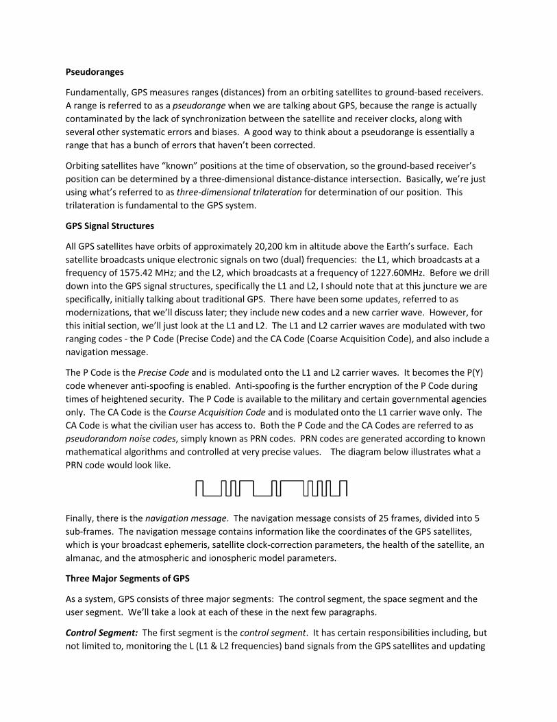
The P Code is the Precise Code and is modulated onto the L1 and L2 carrier waves. It becomes the P(Y) code whenever anti-spoofing is enabled. Anti-spoofing is the further encryption of the P Code during times of heightened security. The P Code is available to the military and certain governmental agencies only. The CA Code is the Course Acquisition Code and is modulated onto the L1 carrier wave only. The CA Code is what the civilian user has access to. Both the P Code and the CA Codes are referred to as pseudorandom noise codes, simply known as PRN codes. PRN codes are generated according to known mathematical algorithms and controlled at very precise values. The diagram below illustrates what a PRN code would look like.

Finally, there is the navigation message. The navigation message consists of 25 frames, divided into 5 sub-frames. The navigation message contains information like the coordinates of the GPS satellites, which is your broadcast ephemeris, satellite clock-correction parameters, the health of the satellite, an almanac, and the atmospheric and ionospheric model parameters.

Three Major Segments of GPS

As a system, GPS consists of three major segments: The control segment, the space segment and the user segment. We’ll take a look at each of these in the next few paragraphs.

Control Segment: The first segment is the control segment. It has certain responsibilities including, but not limited to, monitoring the L (L1 & L2 frequencies) band signals from the GPS satellites and updating

their navigation message. This segment also monitors the satellite’s health and tracks the satellite’s maneuvers.

The control segment consists of five monitoring and two control stations. The first control station is the Master Control Station (MCS) located at the Consolidated Space Operations Center at Schriever Air Force Base near Colorado Springs, Colorado. Second, there’s a backup MCS at Gaithersburg, Maryland. The five monitoring stations are located at Ascension Island, Diego Garcia, Hawaii, Kwajalein Atoll and Cape Canaveral.

Together, the monitoring stations monitor all of the GPS satellites in view and collect ranging and satellite clock data from all available satellites. They then pass this information on to the master control station (MCS). Operators in the master control station then update each satellite’s status, ephemeris, and clock data.

There are two important ephemerides that we need to be aware of; the first is the broadcast ephemeris, and the second is the precise ephemeris. The broadcast ephemeris is the predicted location of where a GPS satellite’s at. Recall that we’re using this location as our control station and even though it’s a predicted location, it’s what we get in real time. It’s important, however, to note that even though these predictions are quite precise, it’s still a prediction. The precise ephemeris on the other hand is the actual location of where the satellite was at. There is an approximate 12 day latency with the precise ephemeris, however, in real precise GPS work you need to be using the precise ephemeris (http://igscb.jpl.nasa.gov/components/prods_cb.html

Space Segment: The second major segment of GPS is the space segment. It consists of 24 Earth-orbiting satellites, made up of 21 operational with 3 spares. As of August 25, 2017 there are 31 orbiting satellites in the GPS system. The satellites are in 6 orbital planes, as mentioned earlier, inclined 55 degrees to the equator. They are at an approximate altitude of 20,200 km above Earth’s surface and have an orbital period of 12 sidereal hours. This means that they come back over the same point approximately every 12 hours. With an orbital period of 12 sidereal hours you’ll have the same satellite in view for approximately 4-5 hours.

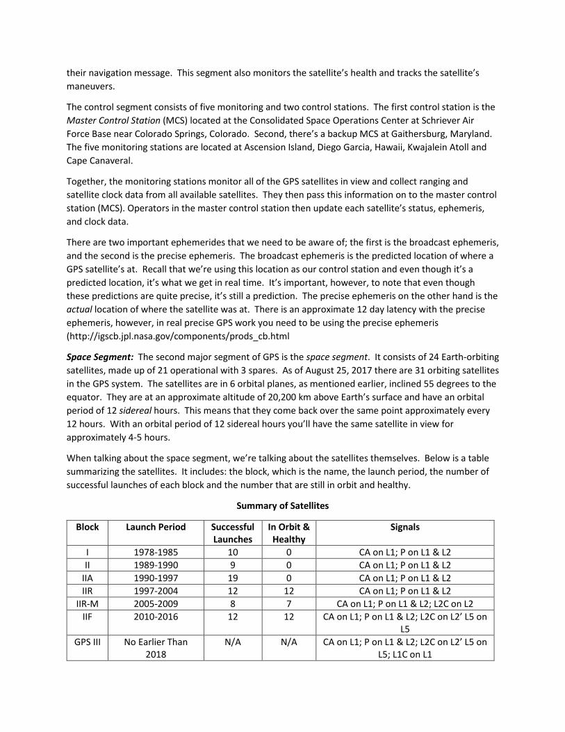
When talking about the space segment, we’re talking about the satellites themselves. Below is a table summarizing the satellites. It includes: the block, which is the name, the launch period, the number of successful launches of each block and the number that are still in orbit and healthy.

Summary of Satellites

Block Launch Period Successful Launches

In Orbit & Healthy

Signals

I 1978-1985 10 0 CA on L1; P on L1 & L2 II 1989-1990 9 0 CA on L1; P on L1 & L2

IIA 1990-1997 19 0 CA on L1; P on L1 & L2 IIR 1997-2004 12 12 CA on L1; P on L1 & L2

IIR-M 2005-2009 8 7 CA on L1; P on L1 & L2; L2C on L2 IIF 2010-2016 12 12 CA on L1; P on L1 & L2; L2C on L2’ L5 on

L5 GPS III No Earlier Than

2018 N/A N/A CA on L1; P on L1 & L2; L2C on L2’ L5 on

L5; L1C on L1

User Segment: The user segment consists of military and civilian users. There are two different types of positioning services available depending on what type of user you’re classified as: Standard Positioning Service (SPS) and the Precise Positioning Service (PPS).

The Standard Positioning Service (SPS), available to civilian users with receivers, is capable of observing the CA code on the L1 frequency only. These types of receivers are classified as single frequency code based receivers.

The second service is the Precise Positioning Service (PPS). It’s available to the military and certain approved governmental agencies. These users are using receivers capable of receiving the CA and the P codes on the L1 and L2 frequencies. These type of receivers are classified as dual frequency code based receivers.

Conceptual GPS in Five Basic Steps

The basic conceptual principals behind GPS are fairly simple. Distances are determined by making measurements using the L1 and L2 frequencies. Now, there’s two forms of positioning that are possible: positioning by pseudorange, also known as point positioning, and positioning by carrier phase. What we’ll try to do in the next few sections is break this system down into five conceptual components. We’ll cover positioning by pseudorange first, and then cover specific things to do with positioning by carrier phase. As we drill down into these, you’ll see many of the components of positioning by pseudorange are also applicable to positioning with carrier phase.

This image represents the five conceptual components of GPS:

Step One – The Basic Idea of Satellite Ranging

To reiterate something mentioned earlier, GPS is based on satellite pseudoranging. Pseudoranging is the range that represents the distance from the satellite to the receiver, and it’s a pseudorange because it has a bunch of uncorrected errors and biases in it.

The satellites serve as our control points for resolving the unknown position of our receiver. Again, it’s important to note that we have a three-dimensional trilateration that’s being performed here. This is the basic idea of satellite ranging.

Below are a few diagrams that’ll help illustrate the concept of trilateration with GPS. The first illustrates a satellite with a sphere drawn around it:

The radius of the sphere is equal to the pseudorange. In this case, we note it as 20,200km. We know that, with this one satellite, that we’re somewhere on this sphere at this radius from this satellite.

Now, let’s look at a scenario with two satellites – we have Satellite I with Sphere I and Satellite II with Sphere II. The radius of each sphere is equal to the pseudorange from the satellite to our receiver. By having two intersecting spheres with a satellite at the center of each sphere, we have two pseudoranges. This knowledge allows us to narrow down where we’re at to the overlap shown in black.

Let’s build upon this and look at another scenario –assume we have three satellites.

In this scenario, we create three spheres around three individual satellites, whose radius is equal to the pseudorange from each satellite to the receiver. By analyzing the geometry of this, we know that where the three spheres intersect will be two points of intersection shown as red dots. Typically, one of these red dots will not be on Earth and can be rejected as a ridiculous answer. We should note, however, that this is not exactly how GPS works. However, fundamentally, you can see that by using three satellites we can narrow down our position to one of two points.

Algebra says that we, in fact, need four satellite pseudoranges to locate our receiver since we need to solve for four simultaneous equations – solving for for: x, y, z and t (time). We’ll cover time in more detail later. This concept is important and relates back to the importance of having a 24 satellite system for full constellation, and being able to track four satellites from any one location around the world. This is necessary since we have four simultaneous equations that we need to solve for – four unknowns mean we need four pseudoranges. We could get by with just three, if we’re able to reject the position that’s not on Earth, if that occurs, but to be safe we want to have the four.

Step Two – Measuring Distance from a Satellite

In step one, we discussed how GPS uses four pseudoranges to come up with the position of a receiver here on Earth. The question arises - how does it come up with the pseudorange? GPS works by timing how long a radio signal takes to reach a receiver from a satellite and then calculating the pseudorange (distance) from that change of time. Radio waves travel at the speed of light in a vacuum - this is 299,792,458 meters per second. For the moment, although not necessarily a true assumption which we’ll address later, let’s assume it’s in a vacuum. If we can figure out exactly what time the GPS satellite started transmitting the radio signal, and then figure out what time it was received at the receiver, we can come up with that change of time. Using the equation: Distance = Speed of Light X Time, we can calculate the pseudorange.

The next question that comes to mind is - How do we know when the signal left the satellite? The Department of Defense came up with the clever idea of synchronizing the satellites and receivers so they are generating the same PRN code at the exact same time. See image below to illustrate this:

In this scenario, the satellite is transmitting a PRN code, a receiver is receiving the PRN code from the satellite, but you also have the receiver generating an internal PRN code. When the receiver compares the PRN code received from the satellite to the one that it generated internally, it’s misaligned. From this misalignment it’s actually able to determine the time difference. With this time difference, we can now say: Time Difference X Speed of Light = Distance, which is the pseudorange.

Step Three – Getting Perfect Timing

Getting perfect timing isn’t possible, so what do we do? Let’s consider a scenario with a satellite and a receiver that are out of sync by 1/100th of a second - our distance would be in error by 2,997,924.58 meters (~1,862 miles). As you can see in this example, the timing issue is really important, so we deal with this by returning back to algebra. Algebra says that if three perfect measurements locate a point in three dimensional space, then four imperfect measurements can eliminate timing offsets. This is why we need four simultaneous equations, which we can get by having four satellites. So, we need four pseudoranges (distances from our 4 satellites) so we can solve for x, y, z and t (time).

Step Four – Knowing Where a Satellite Is In Space

Step four addresses the question of - How do we know where the satellite is? That information is contained in the navigation message; it’s in the form of a broadcast ephemeris and an almanac. An ephemeris is the coordinates of a specific satellite as a function of time.

There are two types of ephemerides that we are concerned with and that we will cover in this course: Broadcast ephemeris and precise ephemeris. While the almanac allows the receiver to quickly find other satellites to use as part of the solution, the data in the almanac is not as precise as the data contained in the broadcast ephemeris. So, once the receiver locks onto the other satellites, it obtains the more precise coordinates of each of those satellites from their individual broadcast ephemerides.

Step Five – Ionospheric and Atmospheric Delays

Step five addresses Ionospheric and Atmospheric delays. There are two specific error sources that are encountered by the GPS signal on its trip from the satellite to the receiver: the ionosphere and the Earth’s atmosphere. The particles encountered during the trip through these two mediums affect the

speed of light, therefore, they affect the GPS signal. Remember that the speed of light is a constant only in a vacuum.

As discussed earlier on, we’re making an assumption that the GPS signal is moving at the speed of light when it really isn’t. When light passes through a denser medium, it slows down. This slowing down has a direct effect on our pseudorange computations.

Now, we’ll spend a moment focusing on the ionosphere. When using single frequency GPS, we do something called single frequency modeling. We’re doing this in an effort to help mitigate the effects of the ionosphere. When using single frequency GPS, we predict what a typical speed variation will be on an average day, under average ionospheric conditions, and then apply that correction factor to all of our measurements. The problem with this type of modeling is that not every day is average. So, therefore, you still have quite a bit of error when using single frequency GPS.

Dual Frequency Ionospheric Free Solution: In terms of the ionosphere, we are much better off using dual frequency because we can come up with something called a dual frequency ionospheric free solution. Essentially, we can measure the variation and the speed of our signal by looking at the relative speed on two different frequencies, L1 and L2. When light travels through the ionosphere it slows down at a rate inversely proportional to its frequency squared. This kind of error correction is only available when using dual frequency GPS receivers.

Atmospheric Delay: In this section we’ll talk a little bit about the delay caused by Earth’s atmosphere. After the GPS signal makes its way through the ionosphere, it enters the Earth’s atmosphere where all of the weather’s contained. Unfortunately, water vapor in the atmosphere can also adversely affect the GPS signal. This error is similar in magnitude to those caused by the ionosphere but, unfortunately, it’s almost impossible to correct for, even with dual frequency. All we can do is model atmospheric delay.

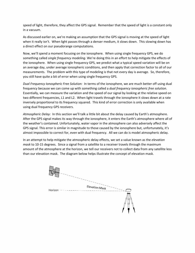
In an attempt to help mitigate the atmospheric delay effects, we set a value known as the elevation mask to 10-15 degrees. Since a signal from a satellite to a receiver travels through the maximum amount of the atmosphere at the horizon, we tell our receivers not to collect data from any satellite less than our elevation mask. The diagram below helps illustrate the concept of elevation mask.

Here you can see that the horizontal line is the horizon, the slope line is the minimum elevation of a satellite that our receiver will track based on what we told it, and the angle between the two lines is our elevation mask angle. It’s recommended that you always check the elevation mask value in your data collector and your baseline processing software.

Another potential error source I want to cover, as part of step five, is from the geometric positioning of the satellites involved in our solution called dilution of precision (DOP). The solution derived from GPS can be better or worse depending on the geometry of your satellites. You can think of this as a strength of figures issue. Errors themselves are not directly increased by the DOP factor, it is the uncertainty in the GPS position that is increased by the DOP factor. A low DOP factor is good, while a high DOP factor is bad. If you’re getting DOP factors above five, to mitigate errors, you may want to take a break and wait for the satellite configuration to change to start your GPS work again.

See below two illustrations that demonstrate what satellite configurations would look like to produce a good DOP factor and a bad DOP factor.

This represents a satellite configuration that would produce a good DOP factor. You can see that the satellites are spread out well across the sky, and you have elevation mask of greater than 10-15 degrees for all of the satellites.

Scenario with a good DOP factor

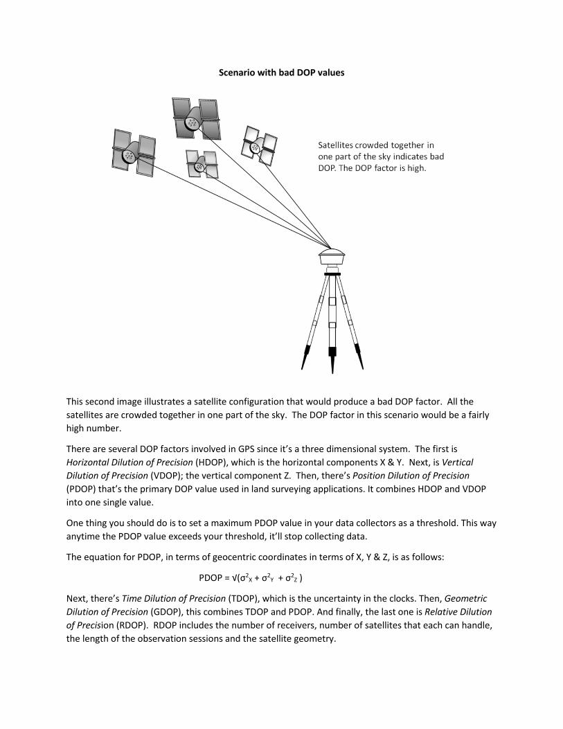
Scenario with bad DOP values

This second image illustrates a satellite configuration that would produce a bad DOP factor. All the satellites are crowded together in one part of the sky. The DOP factor in this scenario would be a fairly high number.

There are several DOP factors involved in GPS since it’s a three dimensional system. The first is Horizontal Dilution of Precision (HDOP), which is the horizontal components X & Y. Next, is Vertical Dilution of Precision (VDOP); the vertical component Z. Then, there’s Position Dilution of Precision (PDOP) that’s the primary DOP value used in land surveying applications. It combines HDOP and VDOP into one single value.

One thing you should do is to set a maximum PDOP value in your data collectors as a threshold. This way anytime the PDOP value exceeds your threshold, it’ll stop collecting data.

The equation for PDOP, in terms of geocentric coordinates in terms of X, Y & Z, is as follows:

PDOP = √(σ2X + σ2

Y + σ2Z )

Next, there’s Time Dilution of Precision (TDOP), which is the uncertainty in the clocks. Then, Geometric Dilution of Precision (GDOP), this combines TDOP and PDOP. And finally, the last one is Relative Dilution of Precision (RDOP). RDOP includes the number of receivers, number of satellites that each can handle, the length of the observation sessions and the satellite geometry.

Another potential error source that is not a factor at this juncture, but could become a factor should the government deem it necessary to turn it back on, it’s called Selective Availability (SA). SA is the intentional degradation of the satellite signal by dithering the satellite clocks. We’ve discussed quite a bit about timing and its importance in GPS; so by messing with the timing you can see how it could really affect the pseudoranges. It was turned off by Presidential Order (President Clinton) on May 2, 2000.

Autonomous GPS-derived positioning, using the CA code alone, has an estimated accuracy of ±100 meters horizontally at the 95% confidence level when SA is turned on. SA of course doesn’t affect the P code, since it’s a restricted military code. The good news is that, from a surveying perspective, it never has and doesn’t affect carrier phase positioning even if it is turned back on.

The last potential error source that I want to cover is referred to as multipath. Multipath occurs when the GPS signal reaches a receiver after reflecting / bouncing off of another object. This causes the pseudorange to be longer than it should be. See diagram below to illustrate this.

The dashed line is the true pseudorange, while the solid line is the pseudorange that’s being received by the receiver after bouncing off the reflective object. As you can see, the signal that’s gone through the path of multipath is longer than what the true pseudorange is. Of course, this affects your positioning.

Multipath & Pseudorange

Carrier Phase GPS

In this section we’ll cover carrier phase ranging. Everything that we’ve covered in the five conceptual steps of GPS thus far is applicable to carrier phase ranging as well, except for SA and the way that the actual range is determined between pseudorange positioning and carrier phase ranging.

Carrier phase ranging is the observable at the center of high accuracy surveying applications using GPS. Observable, in this case, indicates the signal whose measurements yields the range (distance) between the satellite and the receiver. Carrier phase ranging uses the unmodulated L1 and L2 carrier wave lengths, so it’s stripping all the information off the wave length – just using the sinusoidal wave length itself. The foundation is the combination of the unmodulated Doppler shifted carrier, received from a GPS satellite, with the replica of that carrier generated within that receiver.

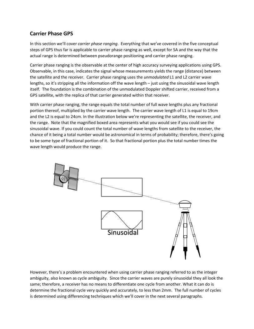
With carrier phase ranging, the range equals the total number of full wave lengths plus any fractional portion thereof, multiplied by the carrier wave length. The carrier wave length of L1 is equal to 19cm and the L2 is equal to 24cm. In the illustration below we’re representing the satellite, the receiver, and the range. Note that the magnified boxed area represents what you would see if you could see the sinusoidal wave. If you could count the total number of wave lengths from satellite to the receiver, the chance of it being a total number would be astronomical in terms of probability; therefore, there’s going to be some type of fractional portion of it. So that fractional portion plus the total number times the wave length would produce the range.

However, there’s a problem encountered when using carrier phase ranging referred to as the integer ambiguity, also known as cycle ambiguity. Since the carrier waves are purely sinusoidal they all look the same; therefore, a receiver has no means to differentiate one cycle from another. What it can do is determine the fractional cycle very quickly and accurately, to less than 2mm. The full number of cycles is determined using differencing techniques which we’ll cover in the next several paragraphs.

Sinusoidal

Types of GPS Differencing Techniques

There are three types of differencing techniques that are used to determine and differentiate cycles: a single difference, double difference and a triple difference.

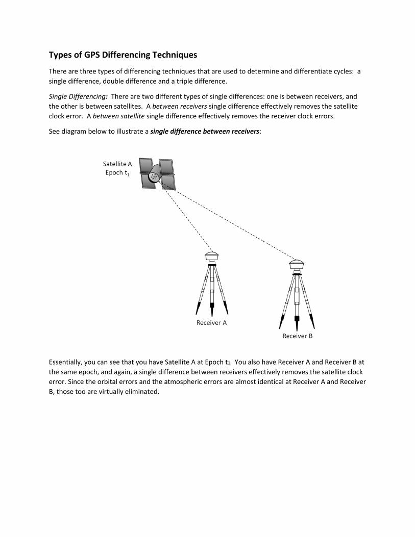
Single Differencing: There are two different types of single differences: one is between receivers, and the other is between satellites. A between receivers single difference effectively removes the satellite clock error. A between satellite single difference effectively removes the receiver clock errors.

See diagram below to illustrate a single difference between receivers:

Essentially, you can see that you have Satellite A at Epoch t1. You also have Receiver A and Receiver B at the same epoch, and again, a single difference between receivers effectively removes the satellite clock error. Since the orbital errors and the atmospheric errors are almost identical at Receiver A and Receiver B, those too are virtually eliminated.

The above diagram illustrates a single difference between satellites. Here, you have Satellite A and Satellite B, both at Epoch t1 (time). Additionally, you have one receiver, Receiver A. Here, a between satellite single difference effectively removes the receiver clock error.

Single Difference Between Satellites

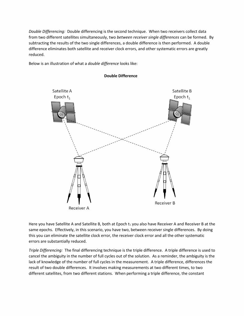
Double Differencing: Double differencing is the second technique. When two receivers collect data from two different satellites simultaneously, two between receiver single differences can be formed. By subtracting the results of the two single differences, a double difference is then performed. A double difference eliminates both satellite and receiver clock errors, and other systematic errors are greatly reduced.

Below is an illustration of what a double difference looks like:

Here you have Satellite A and Satellite B, both at Epoch t1, you also have Receiver A and Receiver B at the same epochs. Effectively, in this scenario, you have two, between receiver single differences. By doing this you can eliminate the satellite clock error, the receiver clock error and all the other systematic errors are substantially reduced.

Triple Differencing: The final differencing technique is the triple difference. A triple difference is used to cancel the ambiguity in the number of full cycles out of the solution. As a reminder, the ambiguity is the lack of knowledge of the number of full cycles in the measurement. A triple difference, differences the result of two double differences. It involves making measurements at two different times, to two different satellites, from two different stations. When performing a triple difference, the constant

Double Difference

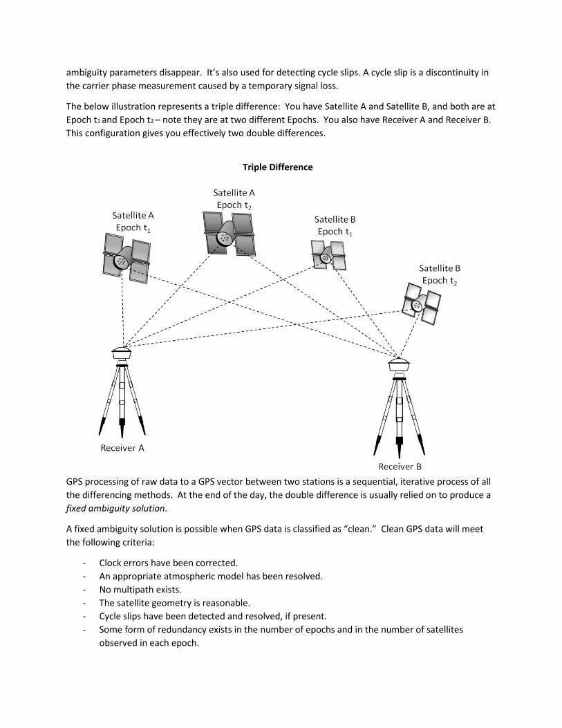
ambiguity parameters disappear. It’s also used for detecting cycle slips. A cycle slip is a discontinuity in the carrier phase measurement caused by a temporary signal loss.

The below illustration represents a triple difference: You have Satellite A and Satellite B, and both are at Epoch t1 and Epoch t2 – note they are at two different Epochs. You also have Receiver A and Receiver B. This configuration gives you effectively two double differences.

GPS processing of raw data to a GPS vector between two stations is a sequential, iterative process of all the differencing methods. At the end of the day, the double difference is usually relied on to produce a fixed ambiguity solution.

A fixed ambiguity solution is possible when GPS data is classified as “clean.” Clean GPS data will meet the following criteria:

- Clock errors have been corrected. - An appropriate atmospheric model has been resolved. - No multipath exists. - The satellite geometry is reasonable. - Cycle slips have been detected and resolved, if present. - Some form of redundancy exists in the number of epochs and in the number of satellites

observed in each epoch.

Triple Difference

Chapter II

Geodesy & State Plane Coordinates

Prior to the advent of GPS, most individuals didn’t have a working knowledge of geodesy or map projections. Now, with so many professionals working with GPS (GNSS) on a regular basis, they need to possess a fundamental understanding of geodesy, as well as map projections. This chapter will review key, fundamental concepts of geodesy and map projections

Geodetic Surfaces

In dealing with GPS, there are three separate but interrelated geodetic surfaces that we need to be concerned with: the ellipsoid, the real earth and the geoid. In the next few sections, we’ll take a look at each of these.

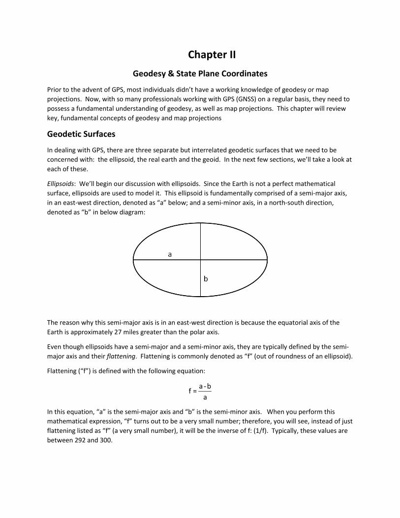
Ellipsoids: We’ll begin our discussion with ellipsoids. Since the Earth is not a perfect mathematical surface, ellipsoids are used to model it. This ellipsoid is fundamentally comprised of a semi-major axis, in an east-west direction, denoted as “a” below; and a semi-minor axis, in a north-south direction, denoted as “b” in below diagram:

The reason why this semi-major axis is in an east-west direction is because the equatorial axis of the Earth is approximately 27 miles greater than the polar axis.

Even though ellipsoids have a semi-major and a semi-minor axis, they are typically defined by the semi-major axis and their flattening. Flattening is commonly denoted as “f” (out of roundness of an ellipsoid).

Flattening (“f”) is defined with the following equation:

aba=f -

In this equation, “a” is the semi-major axis and “b” is the semi-minor axis. When you perform this mathematical expression, “f” turns out to be a very small number; therefore, you will see, instead of just flattening listed as “f” (a very small number), it will be the inverse of f: (1/f). Typically, these values are between 292 and 300.

Three Primary Ellipsoids

The three primary ellipsoids that we need to be concerned with in the US are: the Clarke Ellipsoid of 1866, the Geodetic Reference System Ellipsoid of 1980 and the World Geodetic System Ellipsoid of 1984.

Clarke Ellipsoid of 1866: The Clarke Ellipsoid of 1866 has a semi-major axis:

a = 6,378,206.4m

And an inverse flattening value of:

1/f = 294.978698214

This was the first ellipsoid consistently used in North America, and is the reference ellipsoid for the NAD27 horizontal datum.

Geodetic Reference System Ellipsoid of 1980: The second ellipsoid that we need to be concerned with is the Geodetic Reference System Ellipsoid of 1980, commonly referred to as the GRS80 Ellipsoid.

It has a semi-major axis of:

a = 6,378,137.0m

It has an inverse flattening of:

1/f = 298.25722210088

It’s used for all of the NAD83 horizontal datums including the first realization in 1986, the HARNs, NSRS2007, CORS96, and the most current realization that carries a datum tag of 2011.

It’s also the ellipsoid that was adopted by the International Association of Geodesy.

World Geodetic System Ellipsoid of 1984: Finally, the third ellipsoid that we need to be concerned with is the World Geodetic System Ellipsoid of 1984. This is commonly referred to as the WGS84 Ellipsoid. As mentioned in the introductory chapter, the WGS84 ellipsoid is what’s used by GPS.

Its semi-major axis is:

a = 6,378,137.0m

Its inverse flattening is:

1/f = 298.257223563

One of the special designs of GPS is that the WGS84 datum, which uses the WGS84 ellipsoid, is fixed with the center of the ellipsoid at the Earth’s center of mass. This design allowed for the creation of a truly Earth-centered, Earth-fixed coordinate (ECEF) system, with 0, 0, 0 being coincident with the Earth’s center of mass. This means that the positive X axis is in the equator, toward 0⁰ longitude. The positive Y axis is in the equator, toward 90 ⁰ east longitude. The positive Z axis is up toward the North Pole.

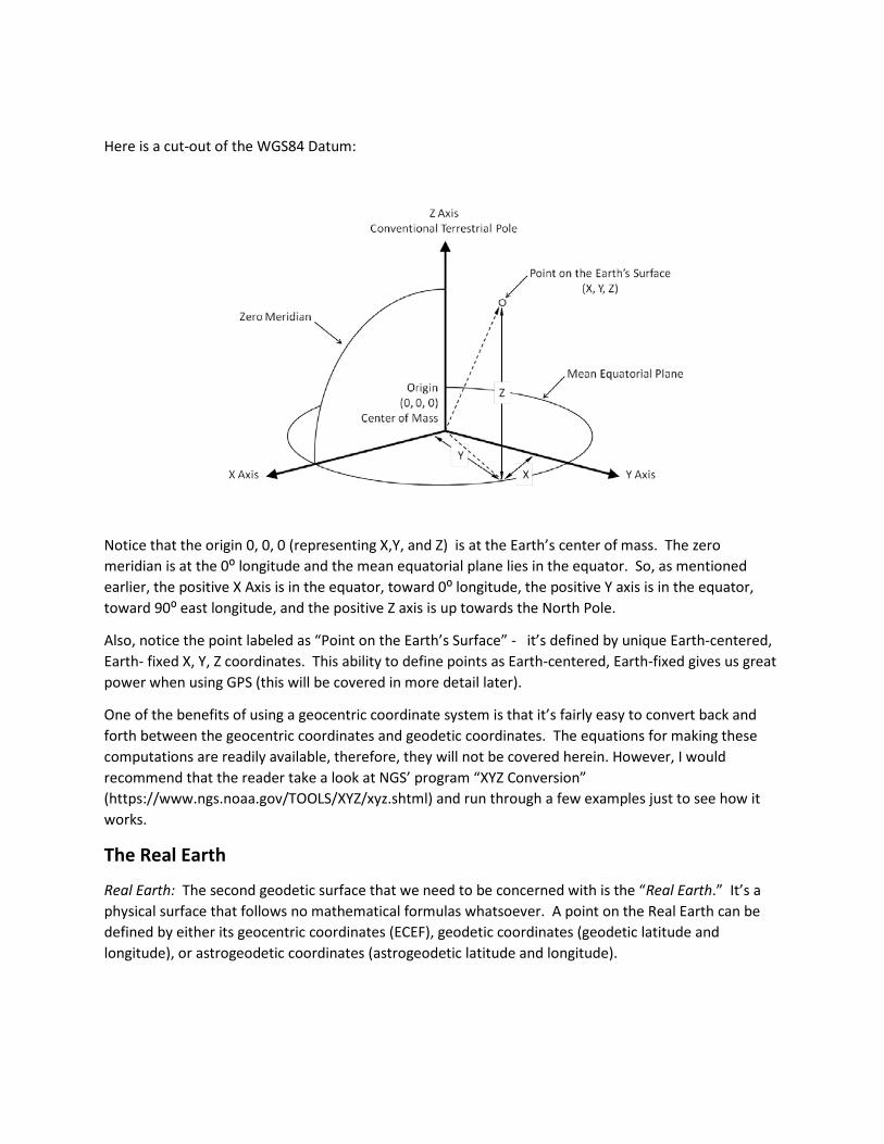
Here is a cut-out of the WGS84 Datum:

Notice that the origin 0, 0, 0 (representing X,Y, and Z) is at the Earth’s center of mass. The zero meridian is at the 0⁰ longitude and the mean equatorial plane lies in the equator. So, as mentioned earlier, the positive X Axis is in the equator, toward 0⁰ longitude, the positive Y axis is in the equator, toward 90⁰ east longitude, and the positive Z axis is up towards the North Pole.

Also, notice the point labeled as “Point on the Earth’s Surface” - it’s defined by unique Earth-centered, Earth- fixed X, Y, Z coordinates. This ability to define points as Earth-centered, Earth-fixed gives us great power when using GPS (this will be covered in more detail later).

One of the benefits of using a geocentric coordinate system is that it’s fairly easy to convert back and forth between the geocentric coordinates and geodetic coordinates. The equations for making these computations are readily available, therefore, they will not be covered herein. However, I would recommend that the reader take a look at NGS’ program “XYZ Conversion” (https://www.ngs.noaa.gov/TOOLS/XYZ/xyz.shtml) and run through a few examples just to see how it works.

The Real Earth

Real Earth: The second geodetic surface that we need to be concerned with is the “Real Earth.” It’s a physical surface that follows no mathematical formulas whatsoever. A point on the Real Earth can be defined by either its geocentric coordinates (ECEF), geodetic coordinates (geodetic latitude and longitude), or astrogeodetic coordinates (astrogeodetic latitude and longitude).

The Geoid

Geoid: The third and final geodetic surface that we need to be concerned with in this discussion is the geoid. The geoid is an equipotential surface, meaning it’s a surface that’s perpendicular to the direction of gravity at all points. Like the Real Earth, a geoid can only be approximated by mathematics, not perfectly defined by one set of mathematical equations. Drilling down into the geoid; we have orthometric and ellipsoidal heights. The relationship between these two are defined by geoid – ellipsoid separations (geoid heights). We have models like Geoid 03, Geoid 09, Geoid 12, Geoid 12A, and Geoid12B, but it’s important to keep in mind that these are models. Since it can’t be perfectly defined by a set of mathematics, all we can do is model this surface. It’s important to always keep in mind that there is a certain amount of error inherent in any geoid model.

The Relationship between the Three Surfaces

Now, let’s take a look at the relationships between the three geodetic surfaces we covered. The relationship between the ellipsoid and the Real Earth is relatively straightforward. Any point on the Earth can have an ellipsoid normal drawn to it. This allows us to compute latitude, longitude and ellipsoidal heights. We refer to these as geodetic coordinates.

The relationship between the Real Earth and the geoid is a bit more complicated because the direction of gravity is perpendicular to the geoid, not perpendicular to the Real Earth. However, the perpendicular can be extended to an intersection with the Real Earth.

The relationship between the ellipsoid and the geoid is defined by two values: geoid height and deflection of the vertical. We’ll cover geoid height in more detail when we get to vertical datums later in this chapter. For right this moment, just keep in mind that it is one of these two values that define the relationship between the ellipsoid and the geoid. So, to define deflection of the vertical, we’ll begin with a component that can be calculated from it that is referred to as the Laplace Correction. The Laplace Correction is an angular value that defines the relationship between an astronomic azimuth, which is related to the geoid, and a geodetic azimuth, which is related to the ellipsoid. See the diagram below:

Now, on this diagram, we have a portion of an ellipsoid and a geoid drawn. Note that we have the earth center of the geoid and we have the ellipsoid center of the ellipsoid labeled, respectively. Also, note that we have the Equator and the North Pole labeled as well. Now, notice the additional points on the diagram: one perpendicular to the ellipsoid and one perpendicular to the geoid. There is a latitude geodetic and a latitude astronomic noted – these are the subscripts A & G. Remember, an astronomic “A” refers to the geoid, and the “G” geodetic refers to the ellipsoid. As they go up and cross - they cross where it’s labeled “deflection of the vertical in the meridian” – this is what the deflection of the vertical is – it’s the angular difference in a zenith direction.

Horizontal Datums

As we move into discussing horizontal datums in North America, let’s begin with a brief and simple working definition of a datum. A horizontal datum is a series of measurements that fit to some mathematical surface, that we can use to produce coordinates from.

The first major horizontal datum used in the US was the North American Datum of 1927, referred to as NAD27. It was primarily a triangulation network. There was one point (latitude/longitude) held fixed, in Meades Ranch in Kansas, with an azimuth mark to a connected station called Waldo. As mentioned before, the Clarke ellipsoid of 1866 was the ellipsoid used for all of the computations involved in NAD27.

The second horizontal datum that we need to be concerned with is the North American Datum of 1983 (1986). The 1986 is the datum tag and in this instance, refers to the first realization of this datum. In common practice the datum tag for the original realization of NAD83 is not included, therefore, it’s just shown as NAD83. Most of the triangulation from NAD27 and some early GPS went into defining this original realization. In addition, quite a bit of trilateration was included because of the invention of EDMs. It’s important to note, however, that 99.9% of the measurements were from conventional surveying measurement techniques, not GPS. This is an important fact since as GPS became more popular, it was recognized that GPS was more precise than the original values shown on the control monumentation that were derived primarily from conventional surveying techniques. So, at the end of the day, this is what led to the need for the early readjustments of NAD83.

So along came GPS, and all of a sudden you were having to warp your measurements to fit to the control of NAD83. Obviously this was unacceptable; so on a state by state basis, and in conjunction with NGS, there was an initiative referred to as HARN (High Accuracy Reference Network) to perform GPS observations for a readjustment. Typically, the primary participants of this initiative were very large companies and organizations, like utility companies and state DOTs.

The primary task was to perform very long static GPS observations that adhered to very specific guidelines dictated by NGS. All the raw data, not the adjusted data, was submitted to NGS for one big adjustment of all the HARN stations within each state. Since GPS is a 3D measuring system, ellipsoidal heights were included as part of the results from the HARN networks.

Well, this was great until you started working in one state and crossed over into a neighboring state (recall, HARNs were state by state adjustments, not national). Then all of sudden the control from State A didn’t quite match the control from State B. As with before, this wasn’t really acceptable.

The need for a national adjustment was easily recognized, and as before, NGS stepped up with a solution to the problem. This was in the form of a national adjustment referred to as NAD83 (NSRS2007), and then later readjustments referred to as NAD83 (CORS96) and NAD83 (2011) respectively. The last, NAD83 (2011), is the latest readjustment by NGS and is based on the continuously operating reference stations around the country.

The datum associated directly with GPS is the World Geodetic System Datum of 1984 (WGS84) that uses the WGS84 ellipsoid. The current realization is WGS84 (G1762). Where G stands for GPS and 1762 is the GPS week number

The final datum that I’d like to cover is known as the International Terrestrial Reference Frame xy (ITRFxy). The “xy” here refers to a particular year. This is a horizontal datum that recognized that Earth is not a static surface, and that points’ coordinates change annually due to this movement. Therefore, points are assigned velocity estimates and are taken into consideration. The ITRF datum is not a “local” datum (eg. specific to only North America like NAD83 is), but is considered a world datum based on continuously operating base stations around the entire world.

At this juncture there’s some basic relationships that should be brought to light.

1) GPS satellite orbits (ephemeris) are given in IGS08 reference frame. For all surveying applications and for all practical purposes it can be considered identical to ITRF08.

2) ITRF08 for all practical and surveying purposes can be considered identical to WGS84 (G1674) and WGS84 (G1762) at less than the 10cm level.

3) The datum transformation between WGS84 (G1762) [IGS08/ITRF08] and NAD83 (2011) requires the use of translations and rotations in x, y and z; and scale. Plus velocities in x, y and z from the geophysical model NNR - NUVEL - 1A.

4) WGS84 (G1674) and WGS84 (G1762) are aligned, or at least are supposed to be, with ITRF08

With all of these different horizontal datums, it becomes necessary from time to time to perform datum transformations. For most surveyors, it’s obvious that NAD27 and NAD83 are very different datums. For

example, the same point in these two different datums, if just looking at latitude and longitude comparatively, can have a coordinate shift of more than 100 feet.

Whereas NAD83 to HARN is a much smaller shift since both use the same ellipsoid. In contrast, NAD27 and NAD83 used very different ellipsoids. Transformations between HARNs and NAD83 (NSRS2007) will only be in the range of 0-4cm, depending on where you’re at in the country.

However, we need to be concerned and aware of datum transformations beyond just NAD27 to some flavor of NAD83 or between flavors of NAD83. For example, if you’re receiving corrections in ITRF08 from precise point positioning in real time from a source like OmniStar or C-Nav and treat them as equivalent to NAD83 (2011) your derived positions will contain an error of approximately 3.5 feet.

Let’s move on and discuss the mathematics of datum transformations in a basic form. The datum transformation is a 3-dimensional coordinate transformation and are based on the geocentric (ECEF) coordinate system. Depending on the required accuracy of the transformation and availability of parameters a number of datum transformations are in use; however, the most common form is the 7-parameter shift described below.

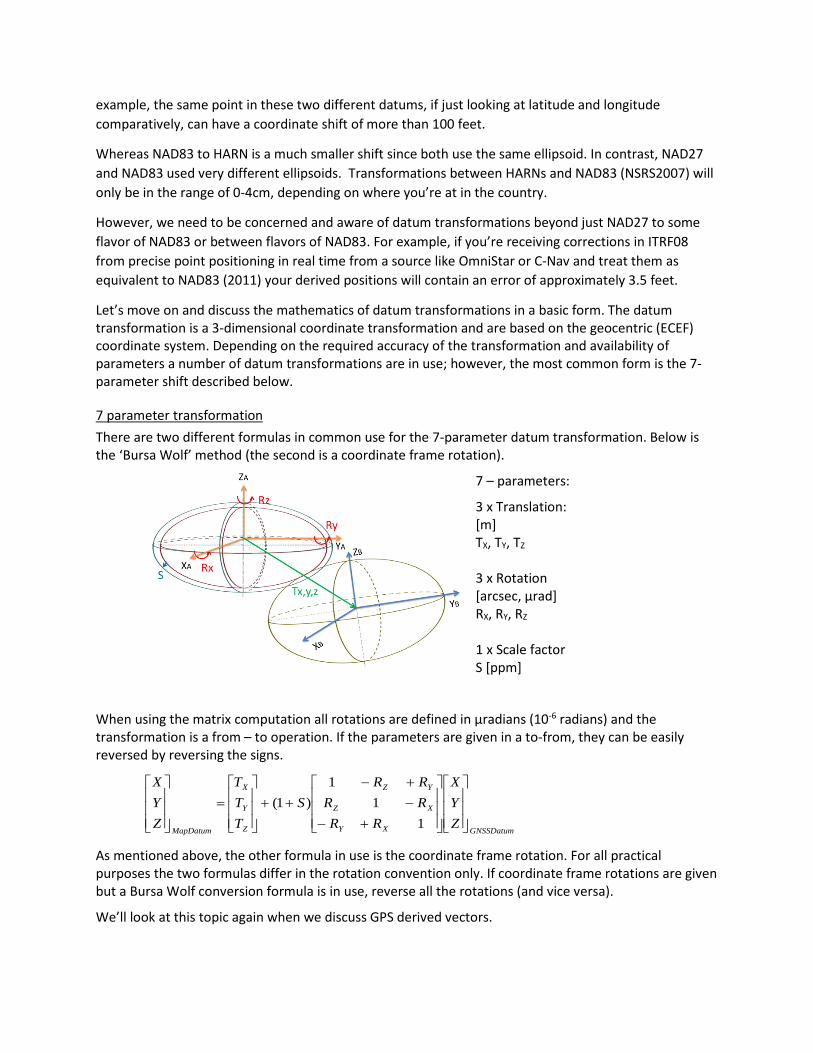
7 parameter transformation There are two different formulas in common use for the 7-parameter datum transformation. Below is the ‘Bursa Wolf’ method (the second is a coordinate frame rotation).

7 – parameters:

3 x Translation: [m] TX, TY, TZ 3 x Rotation [arcsec, μrad] RX, RY, RZ 1 x Scale factor S [ppm]

When using the matrix computation all rotations are defined in μradians (10-6 radians) and the transformation is a from – to operation. If the parameters are given in a to-from, they can be easily reversed by reversing the signs.

GNSSDatumXY

XZ

YZ

Z

Y

X

MapDatumZYX

RRRRRR

STTT

ZYX

+−−+−

++

=

11

1)1(

As mentioned above, the other formula in use is the coordinate frame rotation. For all practical purposes the two formulas differ in the rotation convention only. If coordinate frame rotations are given but a Bursa Wolf conversion formula is in use, reverse all the rotations (and vice versa).

We’ll look at this topic again when we discuss GPS derived vectors.

Vertical Datums

In this section, we’re going to leave horizontal datums and start talking about vertical datums. The two main vertical datums that we’re going to discuss are: NGVD29 and NAVD88. NGVD29 stands for National Geodetic Vertical Datum of 1929 and NAVD88 stands for North American Vertical Datum of 1988.

National Geodetic Vertical Datum of 1929 (NGVD29): In NGVD29, elevation differences were forced to fit mean sea level which is an interesting concept since mean sea level is not a level surface. A good illustration of this is looking at the Florida coasts; the east and west coasts of Florida have a sea level offset of approximately a 0.5’.

North American Vertical Datum of 1988 (NAVD88): As survey technologies became more accurate, it became increasingly apparent that NGVD29 constraints were incorrectly forcing surveys to fit different tide stations (all zero elevation or mean sea level) that actually had different elevations relative to each other.

During the 1970s, NGS, and counterpart agencies in Mexico and Canada, adopted a vertical datum based on a surface that would closely approximate the Earth’s geoid. The new adjustment, NAVD88, was completed in June 1991 and is now the only official vertical datum in the United States. NAVD88 was created by adding 625,000 kilometers of leveling performed after NGVD29 was established, and by performing a major minimally constrained least squares adjustment that constrained a single tide station in Canada.

As noted, in NAVD88, orthometric height differences were used in a least squares analysis where only one benchmark in Canada was held fixed. It’s important to note the introduction of the term orthometric height, instead of elevation differences.

Elevation differences were converted to orthometric height differences since this difference becomes significant when level runs exceed 100 miles. So, what’s the difference between elevation difference and orthometric height difference? Elevation differences do not account for non-parallelism of level surfaces (such as mean sea level used in NGVD29), where orthometric heights do

Any time you have more than one datum, horizontal or vertical, it seems like it becomes necessary at some point and time to do a datum transformation. As mentioned previously, NGS developed a program called NADCON to allow for consistent horizontal datum transformations with the best precision possible. In addition, they also developed a free tool, called VERTCON, for handling vertical datum transformations.

Here are some important points to note about VERTCON:

1) The algorithm is produced by NGS, based on all points with elevations in both datums. 2) A “best fit” is applied to a point between existing NGS stations with elevations in both datums.

This is pretty much restating the prior point but it is important to stress that it’s a best fit, similar to NADCON.

3) Two points, close in distance, will shift the same amounts vertically, and in the same direction typically when using VERTCON.

Geoid Models

We’re going to spend a few moments discussing geoid models. Anytime we cover vertical datums, we want to note that GPS’s native vertical dimension is ellipsoid height, not orthometric height. In order to obtain orthometric heights from ellipsoid heights we need to use a geoid model. Over the years NGS has developed several different geoid models and each one has been replaced with the next revision: They started with Geoid90, and it was followed by Geoid93, Geoid96, Geoid99, Geoid03, Geoid09, Geoid12, Geoid 12A, and the latest is Geoid12B.

Geoid height is negative by definition in the lower 48 states since the geoid is below the ellipsoid. So, if you go out to NGS’ website and put in a latitude / longitude and want a geoid height - it will have a capital “N” and then it will say “= -26.24 meters”, or whatever the case may be. There is an equation that you can memorize that says that the orthometric height is equal to the ellipsoid height, minus the geoid height. Remember, if you are doing this equation, it’s minus a minus (in the lower 48 states), since the geoid height is a negative by definition.

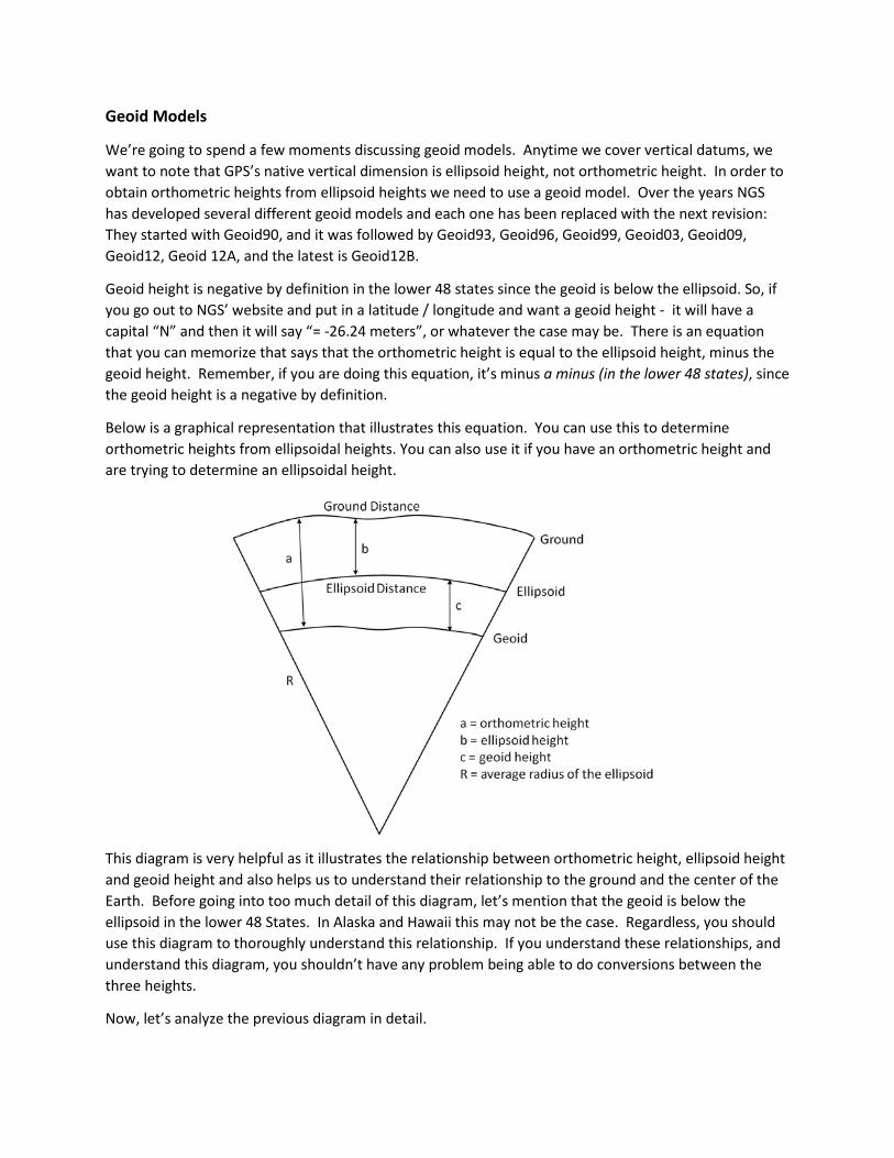
Below is a graphical representation that illustrates this equation. You can use this to determine orthometric heights from ellipsoidal heights. You can also use it if you have an orthometric height and are trying to determine an ellipsoidal height.

This diagram is very helpful as it illustrates the relationship between orthometric height, ellipsoid height and geoid height and also helps us to understand their relationship to the ground and the center of the Earth. Before going into too much detail of this diagram, let’s mention that the geoid is below the ellipsoid in the lower 48 States. In Alaska and Hawaii this may not be the case. Regardless, you should use this diagram to thoroughly understand this relationship. If you understand these relationships, and understand this diagram, you shouldn’t have any problem being able to do conversions between the three heights.

Now, let’s analyze the previous diagram in detail.

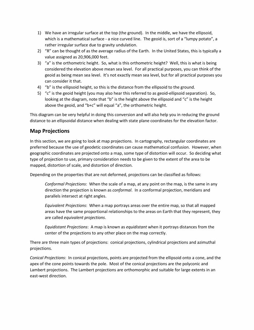
1) We have an irregular surface at the top (the ground). In the middle, we have the ellipsoid, which is a mathematical surface - a nice curved line. The geoid is, sort of a “lumpy potato”, a rather irregular surface due to gravity undulation.

2) “R” can be thought of as the average radius of the Earth. In the United States, this is typically a value assigned as 20,906,000 feet.

3) “a” is the orthometric height. So, what is this orthometric height? Well, this is what is being considered the elevation above mean sea level. For all practical purposes, you can think of the geoid as being mean sea level. It’s not exactly mean sea level, but for all practical purposes you can consider it that.

4) “b” is the ellipsoid height, so this is the distance from the ellipsoid to the ground. 5) “c” is the geoid height (you may also hear this referred to as geoid-ellipsoid separation). So,

looking at the diagram, note that “b” is the height above the ellipsoid and “c” is the height above the geoid, and “b+c” will equal “a”, the orthometric height.

This diagram can be very helpful in doing this conversion and will also help you in reducing the ground distance to an ellipsoidal distance when dealing with state plane coordinates for the elevation factor.

Map Projections

In this section, we are going to look at map projections. In cartography, rectangular coordinates are preferred because the use of geodetic coordinates can cause mathematical confusion. However, when geographic coordinates are projected onto a map, some type of distortion will occur. So deciding what type of projection to use, primary consideration needs to be given to the extent of the area to be mapped, distortion of scale, and distortion of direction.

Depending on the properties that are not deformed, projections can be classified as follows:

Conformal Projections: When the scale of a map, at any point on the map, is the same in any direction the projection is known as conformal. In a conformal projection, meridians and parallels intersect at right angles.

Equivalent Projections: When a map portrays areas over the entire map, so that all mapped areas have the same proportional relationships to the areas on Earth that they represent, they are called equivalent projections.

Equidistant Projections: A map is known as equidistant when it portrays distances from the center of the projections to any other place on the map correctly.

There are three main types of projections: conical projections, cylindrical projections and azimuthal projections.

Conical Projections: In conical projections, points are projected from the ellipsoid onto a cone, and the apex of the cone points towards the pole. Most of the conical projections are the polyconic and Lambert projections. The Lambert projections are orthomorphic and suitable for large extents in an east-west direction.

Cylindrical Projections: In cylindrical projections, points are projected from an ellipsoid onto a cylinder enveloping the ellipsoid. Depending on the orientation, there are three different types of cylindrical projections:

1) Longitudinal: if the cylinder axis is through the poles, it’s longitudinal 2) Transverse: If the cylindrical axis is through the equator, it’s transverse 3) Oblique: If the cylindrical axis is through an arbitrary angle (not longitudinal or transverse), then

it’s referred to as oblique.

The most common cylindrical projections are the Longitudinal Mercator, used for nautical charting; and the Universal Transverse Mercator, known as UTM.

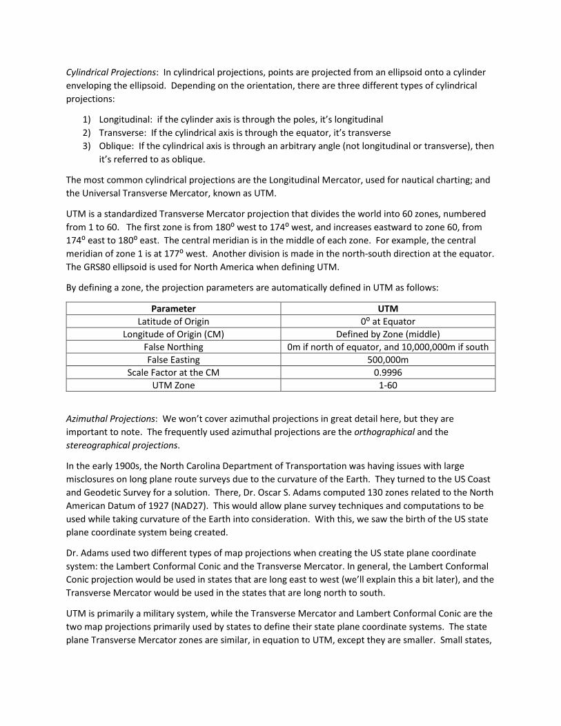
UTM is a standardized Transverse Mercator projection that divides the world into 60 zones, numbered from 1 to 60. The first zone is from 180⁰ west to 174⁰ west, and increases eastward to zone 60, from 174⁰ east to 180⁰ east. The central meridian is in the middle of each zone. For example, the central meridian of zone 1 is at 177⁰ west. Another division is made in the north-south direction at the equator. The GRS80 ellipsoid is used for North America when defining UTM.

By defining a zone, the projection parameters are automatically defined in UTM as follows:

Parameter UTM Latitude of Origin 0⁰ at Equator

Longitude of Origin (CM) Defined by Zone (middle) False Northing 0m if north of equator, and 10,000,000m if south False Easting 500,000m

Scale Factor at the CM 0.9996 UTM Zone 1-60

Azimuthal Projections: We won’t cover azimuthal projections in great detail here, but they are important to note. The frequently used azimuthal projections are the orthographical and the stereographical projections.

In the early 1900s, the North Carolina Department of Transportation was having issues with large misclosures on long plane route surveys due to the curvature of the Earth. They turned to the US Coast and Geodetic Survey for a solution. There, Dr. Oscar S. Adams computed 130 zones related to the North American Datum of 1927 (NAD27). This would allow plane survey techniques and computations to be used while taking curvature of the Earth into consideration. With this, we saw the birth of the US state plane coordinate system being created.

Dr. Adams used two different types of map projections when creating the US state plane coordinate system: the Lambert Conformal Conic and the Transverse Mercator. In general, the Lambert Conformal Conic projection would be used in states that are long east to west (we’ll explain this a bit later), and the Transverse Mercator would be used in the states that are long north to south.

UTM is primarily a military system, while the Transverse Mercator and Lambert Conformal Conic are the two map projections primarily used by states to define their state plane coordinate systems. The state plane Transverse Mercator zones are similar, in equation to UTM, except they are smaller. Small states,

like Vermont, are typically one zone. Larger states, like Florida, can have multiple zones. They are usually used in states that are longer north-south than east-west.

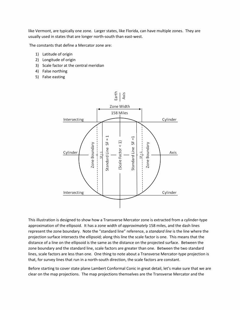
The constants that define a Mercator zone are:

1) Latitude of origin 2) Longitude of origin 3) Scale factor at the central meridian 4) False northing 5) False easting

This illustration is designed to show how a Transverse Mercator zone is extracted from a cylinder-type approximation of the ellipsoid. It has a zone width of approximately 158 miles, and the dash lines represent the zone boundary. Note the “standard line” reference, a standard line is the line where the projection surface intersects the ellipsoid; along this line the scale factor is one. This means that the distance of a line on the ellipsoid is the same as the distance on the projected surface. Between the zone boundary and the standard line, scale factors are greater than one. Between the two standard lines, scale factors are less than one. One thing to note about a Transverse Mercator-type projection is that, for survey lines that run in a north-south direction, the scale factors are constant.

Before starting to cover state plane Lambert Conformal Conic in great detail, let’s make sure that we are clear on the map projections. The map projections themselves are the Transverse Mercator and the

Lambert Conformal Conic. The state plane is the state plane coordinate system that each state has defined, that is used with this particular type of map projection. Now, a state plane Lambert Conformal Conic is extracted from a cone intersecting the ellipsoid. Again, they are normally used for states longer east-west than north-south. So, like in Oklahoma, for example, you have two zones – north and south; and both use the Lambert Conformal Conic as the mapping projection. Larger states are usually multiple zones, smaller states typically have single zones.

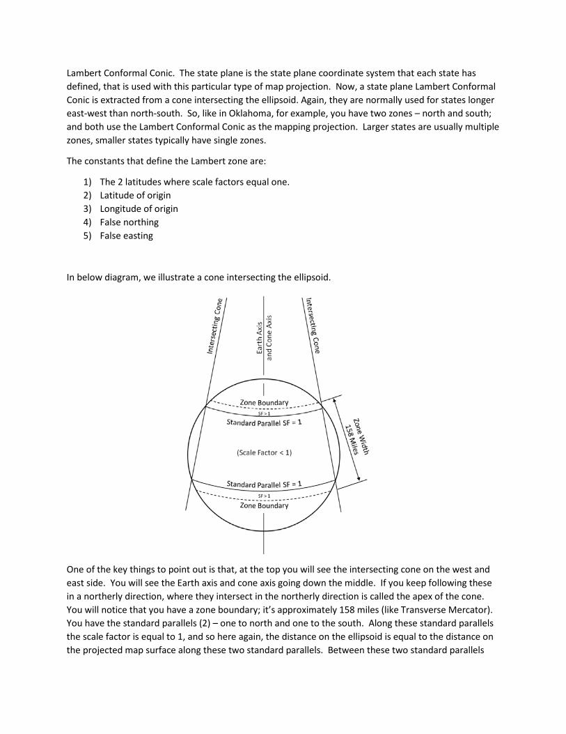
The constants that define the Lambert zone are:

1) The 2 latitudes where scale factors equal one. 2) Latitude of origin 3) Longitude of origin 4) False northing 5) False easting

In below diagram, we illustrate a cone intersecting the ellipsoid.

One of the key things to point out is that, at the top you will see the intersecting cone on the west and east side. You will see the Earth axis and cone axis going down the middle. If you keep following these in a northerly direction, where they intersect in the northerly direction is called the apex of the cone. You will notice that you have a zone boundary; it’s approximately 158 miles (like Transverse Mercator). You have the standard parallels (2) – one to north and one to the south. Along these standard parallels the scale factor is equal to 1, and so here again, the distance on the ellipsoid is equal to the distance on the projected map surface along these two standard parallels. Between these two standard parallels

and the zone boundaries, the scale factors are greater than 1. In between the standard parallels, the scale factor is less than 1. With Lambert, survey lines that run in the east-west direction have scale factors that are constant and north-south direction they are constantly changing.

State Plane Coordinates & Projections

For the remainder of this section, we’ll take a look at some fundamental mathematical principles pertaining to plane projections:

Ellipsoid Factor: The first is the ellipsoid factor (NAD83), known as elevation factor in NAD27. This is the factor that allows us to reduce a ground distance to an ellipsoidal distance.

Scale Factor: The second is the scale factor; this factor allows us to project an ellipsoidal distance to the mapping projection.

Combined Scale Factor: Combined scale factor combines the ellipsoid factor and the scale factor into one to where we aren’t using them separately.

Convergence Angle: Convergence angle is the angular relationship between a grid azimuth and the geodetic azimuth.

Arc to Chord correction: Azimuths that are ran on the Earth are actually curved lines, while with a projection surface they are straight lines. On very long lines, greater than 8 km, and typically for very precise work – you need to reduce this curved line from the Earth itself, to a straight line on the projection surface – hence, this is the arc to chord correction.

Laplace Correction: The last one is the Laplace correction which defines the relationship between a geodetic azimuth and an astronomic azimuth.

We’ll start by looking at the elevation factor in State Plane Coordinate NAD27 and the ellipsoidal factor in state plane coordinate NAD83 (all datum tags). Again, these are essentially the same thing just defined a little differently. Recall that these are the factors that allows us to reduce a ground distance to an ellipsoidal distance. If we start with NAD27, the definition mathematically is:

h+RR

R is the Earth’s average radius, given typically as 20,906,000 ft.

h is the elevation above mean sea level.

Recall that in NAD27 the ellipsoid was best fit to North America, so the ellipsoid is considered coincident with mean sea level in this particular system. There is no geoid height, or you could say no ellipsoid geoid separation, that you have to deal with. You do, however, need to deal with it in NAD83. In NAD83, we’ll call it ellipsoidal factor (vs. elevation factor). Here, you must consider the ellipsoid geoid separation. If you let the same equation apply:

h+RR

You still let R be the Earth’s average radius as 20,906,000 ft., however, you have a new definition of “h”:

h = H+N

Here, lowercase “h” is the ellipsoid height; uppercase “H” is the height above the geoid, and “N” is the geoid height.

It’s important to understand what each one of these factors is doing in the computations - the elevation and ellipsoidal factors, reduce the ground distance to an ellipsoidal distance.

Once you have the elevation factor in NAD27, or the ellipsoid factor in NAD83, and you want to convert a ground distance to an ellipsoidal distance, all you need to do is multiply the ground distance by the ellipsoidal/elevation factor, depending on which system you are working in.

Now, if you have the ellipsoidal distance, and you want the ground distance, all you need to do is divide the ellipsoidal distance by the elevation factor. This is just an algebraic opposite operation.

The second factor we want to cover is the scale factor. As mentioned earlier, this is used to project the ellipsoidal distance to the projection surface. Once the ellipsoidal distance is projected to the map’s surface that distance is referred to as a grid distance. The scale factor is a function of the location in your state plane coordinate zone. The size of the state plane coordinate zone is limited by the scale factor, not exceeding 1 part in 10,000; this means that your scale factors will range from 0.9999 to 1.0001. If you want to project an ellipsoidal distance to a grid distance, you multiply the ellipsoidal distance by the scale factor. You do the opposite if you want to go the other way – so, if you have a grid distance and you want an ellipsoidal distance, you divide by the scale factor.

By using algebraic manipulation, you can come up with a third factor, known as the combined scale factor. All you do is multiply the elevation factor by the scale factor. In this particular scenario, we are saying elevation factor (considering NAD27), but if you were in NAD83 it would be the ellipsoid factor (vs. elevation factor). Once you get the combined scale factor, and you have the horizontal distance and you want to know the grid distance, all you do is multiply the horizontal ground distance by the combined scale factor and you get the grid distance. Conversely, if you have the grid distance and you want the horizontal ground distance, all you do is divide the grid distance by the combined scale factor.

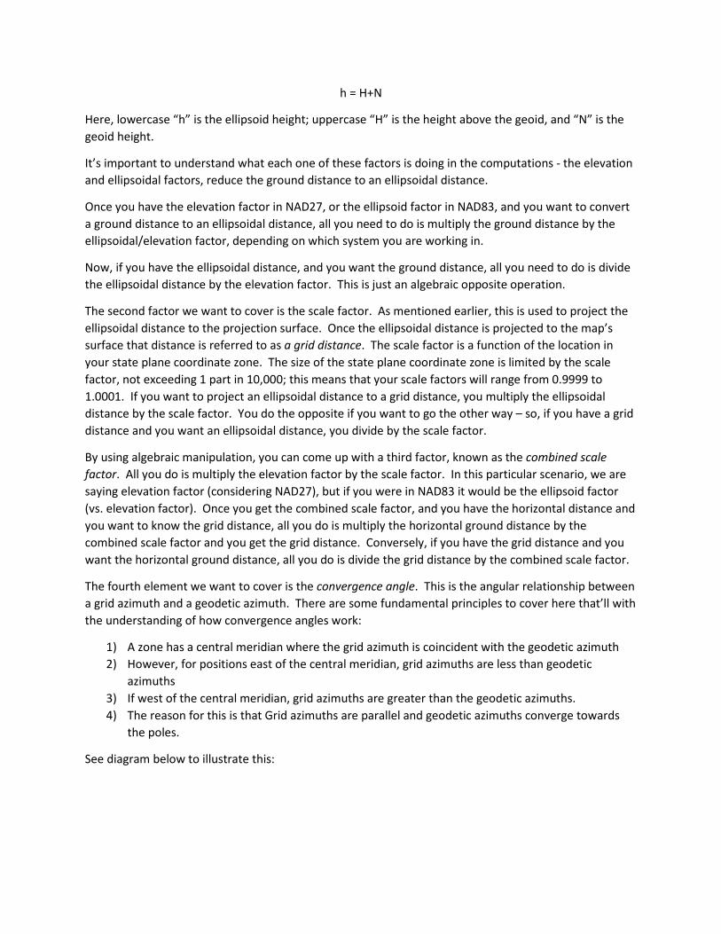
The fourth element we want to cover is the convergence angle. This is the angular relationship between a grid azimuth and a geodetic azimuth. There are some fundamental principles to cover here that’ll with the understanding of how convergence angles work:

1) A zone has a central meridian where the grid azimuth is coincident with the geodetic azimuth 2) However, for positions east of the central meridian, grid azimuths are less than geodetic

azimuths 3) If west of the central meridian, grid azimuths are greater than the geodetic azimuths. 4) The reason for this is that Grid azimuths are parallel and geodetic azimuths converge towards

the poles.

See diagram below to illustrate this:

By examining this diagram, notice we have the central meridian noted as CM. The grid azimuth is equal to the geodetic azimuth along this central meridian. Once we move to the east and west of this central meridian, we see that the grid azimuths are parallel to the central meridian, in a north-south direction. However, we see the geodetic azimuths converging towards the poles. If we let Ɵ represent the convergence angle; if east of the central meridian, the convergence angle is positive; if west of the central meridian, the convergence angle is negative.

Let’s take a look at the equations below for determining the convergence angle; from this you can see the sign convention and how it is derived. There are two different equations for determining the convergence angle, one for the Transverse Mercator system and one for the Lambert Conformal Conic systems.

• ϴ for Transverse Mercator

– ϴ = (λcm – λ)sineΦ

• ϴ for Lambert Conformal Conic

– ϴ = (λcm – λ)sineΦo

» Φo = constant for the particular zone

• Ex. OK S = 34°35’03.11”

From these equation, hopefully you can see where the sign conventions are coming from, in terms of east and west of the central meridian. Also, we hope that you can see that the greater the distance from the central meridian, the greater the difference between the geodetic and the grid azimuths.

Now there is an equation that relates the grid azimuth, the geodetic azimuth and the convergence angle, it’s:

Grid azimuth = Geodetic Azimuth - Convergence angle.

When using this equation, make sure that you pay appropriate attention to the algebraic signs - so if west of the central meridian, you are subtracting a negative (so it’s a positive), and if east of the Central meridian you are subtracting a positive.

We’ve mentioned that a geodetic azimuth and an astronomic azimuth are related by an angular term called the Laplace Correction. The mathematical equation for relating the three is:

Geodetic Azimuth = Astronomic Azimuth + Laplace Correction

You can obtain the Laplace Correction from NGS’ program known as Deflec 12A

See below an example of working through examples relating Astronomic Azimuth, Grid Azimuth and Geodetic Azimuth:

• Let’s say we are given:

– Astronomic Azimuth = 32°04’17”

– Laplace Correction = -14”

– Convergence Angle = +00°18’50”

Note: Since it’s positive it’s east of the central meridian.

• Let’s Solve for:

– Geodetic Azimuth

Recall, the formula for Geodetic Azimuth is:

Geodetic Azimuth = Astronomic Azimuth + Laplace Correction

Solution: Geodetic Azimuth = 32°04’17” + -14” = 32°04’03”

– Grid Azimuth

Recall, the formula for Grid Azimuth is:

Grid Azimuth = Geodetic Azimuth – Convergence Angle

Solution: Grid Azimuth = 32°04’03” – 00°18’50” = 31°45’13”

Finally, we’d be remiss if we didn’t mention that for very long lines, NGS recommends the following method for determining scale factors:

6K+4K+K=K 2m1

21

– K1 = Scale Factor at point 1 (end of line)

– K2 = Scale Factor at point 2 (other end of line)

– Km = Scale Factor at the middle of the line

– K1-2 = Scale Factor for line 1 to 2

Chapter III

GPS Receivers and Techniques Before delving into the different types of GPS techniques we needed to review the basics of geodesy. Now that we’ve gotten past that in chapter two, we’ll be discussing the different types of GPS receivers and techniques available. GPS Receivers There are four specific GPS receivers we’ll be covering: the P Code, CA Code, Single Frequency Carrier Phase, and the Dual Frequency Carrier Phase. We’ll begin by reviewing the P Code receivers. They’re capable of receiving the P and CA Codes, using the L1 and L2 frequencies. They are restricted to the military and certain approved governmental agencies. Next, is the CA Code receiver; it receives the CA Code on the L1 frequency only. These receivers are typically handheld units and are used for things such as: civilian navigation, hunting, fishing and hiking. They are also used as part of a mapping grade GPS technique, referred to as code-based differential GPS (DGPS). Next, we have the single frequency carrier phase GPS receivers. This type of receiver uses the unmodulated L1 carrier wave length. The types of techniques that can be performed with these types of receivers are:

1) Static 2) Kinematic 3) Limited Real Time Kinematic (RTK) 4) Limited Precise Point Positioning (PPP)

The last type of receiver is known as the dual frequency carrier phase receiver. It uses the unmodulated L1 and L2 carrier wave lengths for resolving its position. The type of techniques that can be performed with dual frequency carrier phase GPS are:

1) Static 2) Kinematic 3) Real Time Kinematic (RTK) 4) Rapid Static 5) Pseudokinematic 6) Precise Point Positioning (PPP)

GPS Techniques The first type of GPS technique we’ll cover is the handheld GPS unit that uses the CA Code and requires no office processing. It’s the crudest form of real time GPS point positioning but satisfies 95% of GPS users’ needs. These handhelds generally have extensive background maps and have horizontal accuracies in the 1-30m range.

The second type of GPS technique using the CA Code is referred to as sub-meter Real Time Differential GPS (DGPS) or mapping-grade GPS. It receives a very simple, real-time, 3D correction in an RTCM format, from a public base station via radio connection (RTCM stands for Radio Technical Commission for Maritime format). The correction is based on the base station’s current point position vs. its “known” position. The improved accuracies are made possible by assuming that the same systematic errors exists at the base station as at the rover. The typical systematic errors are satellite orbital errors, GPS clock errors and atmospheric conditions. This assumption is valid when the base and rover are in close proximity; however, it starts to erode in accuracy once the separation exceeds 50 miles. When using DGPS, accuracies in the 1-2 meter range are achievable under good satellite constellation and visibility. There are basically six differential carrier phase GPS surveying techniques that we’ll cover:

1) Static 2) Pseudokinematic 3) Stop and Go Kinematic 4) Kinematic 5) Rapid Static 6) Real Time Kinematic (RTK)

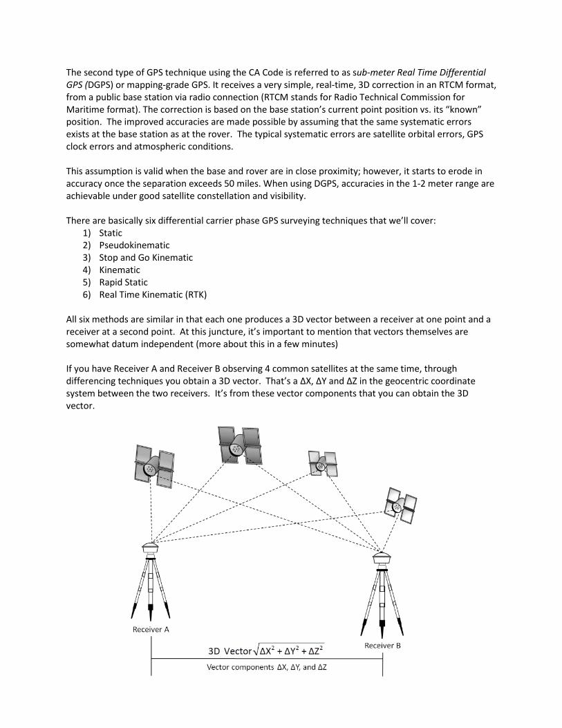
All six methods are similar in that each one produces a 3D vector between a receiver at one point and a receiver at a second point. At this juncture, it’s important to mention that vectors themselves are somewhat datum independent (more about this in a few minutes) If you have Receiver A and Receiver B observing 4 common satellites at the same time, through differencing techniques you obtain a 3D vector. That’s a ΔX, ΔY and ΔZ in the geocentric coordinate system between the two receivers. It’s from these vector components that you can obtain the 3D vector.

One of the most important things to understand in GPS is the dataflow involved. Understanding this process allows one to truly understand how to get the most out of your GPS data. Example of a GPS Data Flow Using Vector Components: To further assist in illustrating this concept, and to illustrate vector addition, let’s review the following example of a GPS data flow using vector components.

1) In this scenario we have a rapid static, two hour occupation: 2) Two Receivers, Collecting Data for Two Hours:

a. Receiver A - occupies control point ALF b. Receiver B - occupies unknown point AIA2

3) Control Point ALF has the following known geodetic coordinates in NAD83 (2011): a. North Latitude, Φ = 35°04’26.04076” (N) b. West Longitude, λ = 90°08’42.19599” (W) c. Ellipsoidal Height, h = 70.9719m

4) The vector components from ALF to AIA2, from differencing techniques from your baseline processing are shown below. Note your change of X, Y and Z (in meters), respectively in bold:

a. ΔX = -1012.8661 0.00002199 -0.00000030 0.00000030 b. ΔY = 9.5556 0.00002806 -0.00000030 c. ΔZ = -35.8575 0.00003640

i. The other terms are your variance – covariance matrix. We’ll discuss this is detail when we discuss least squares adjustments. For now, just be aware that you could see these terms in baseline processing software.

Step 1: The first step in performing a computation is to convert the geodetic coordinates of control station ALF to Earth Centered, Earth-fixed (ECEF) coordinates (same thing as geocentric coordinates). To do this, we’ll use the GRS80 ellipsoid and NGS Geodetic Toolkit program called “XYZ Coordinate Conversion”. Geocentric coordinates of ALF are:

1) XALF = -13229.9712m 2) YALF = -5225761.3343m 3) ZALF = 3644620.5426m

Step 2: Next, we need to perform our vector addition, in our ECEF coordinate system. This vector addition will be from station ALF to station AIA2.

1) X AIA2 = -13229.9712m + -1012.8661m = -14242.8373m 2) Y AIA2 = -5225761.3343m + 9.5556m = -5225751.7787m 3) Z AIA2 = 3644620.5426m + -35.8575m = 3644584.6851m

Step 3: The next step in our coordinate computations is to convert the ECEF coordinates of station AIA2 to geodetic coordinates. Again, we’ll do this on the GRS80 ellipsoid and use NGS’s program, under Geodetic Toolkit known as – XYZ Coordinate Conversion.

1) Φ = 35°04’25.21703” (N) 2) λ = 90°09’22.17534” (W) 3) Ellipsoidal Height, h = 44.7256m

Since we’re typically interested in our final products being delivered in some form of grid coordinates with an orthometric height, let’s continue working through the data flow. Step 4: The next step is to transform the geodetic coordinates (latitude and longitude) to state plane coordinates. We’ll perform this using the NGS’s program, State Plane Coordinates under Geodetic Toolkit.

1) Northing = 90189.709m [295897.40’ (US Survey Feet)] 2) Easting = 221032.511m [725170.83’ (US Survey Feet)]

Please note that since this site is in Tennessee, we want to use their definition of the foot – meter relationship. They use the US survey foot definition, therefore, we’ll convert the northing and easting from meters to US survey feet using that definition. Step 5: Our final step in this GPS data flow is to convert the ellipsoidal height of station AIA2 to an orthometric height. Using NGS Toolkit, program Geoid 12B, we obtain a Geoid height (N) of -27.303m. Using the equation H = h-N, we solve for the orthometric height: 44.756m – (-27.303m) = 72.059m (or 236.41’) Recall that in this equation “H” equals the orthometric height, “h” is the ellipsoidal height and “N” is the geoid height. Again, as seen above, when we substitute everything in, we get an orthometric height (H) of 72.059m, or approximately 236.41 US survey feet. At this juncture, let’s return to our discussion about vectors being somewhat datum independent and why it’s an important concept. The first reason has to do with datum transformations. If you attach a vector, as seen above, to a beginning position, such as a base station, the vector addition will produce the second point in the same datum as the first. It doesn’t really matter if the vector is in WGS84 (Gxxxx) or NAD83 (xxxx). This means that if you enter the base coordinates in NAD83 (2011) and apply a datum transformation from WGS84 (G1762) your end point would no longer be in NAD83 (2011). Therefore, it’s best to focus on what datum your base coordinates are in when possible. The second reason is centered on using your vectors in the future as new ECEF datums are realized. If you have trust and belief in your vectors, just hinge them to the updated control values and re-compute the forward position as above. There really is no reason to re-observe if you have faith in your prior work. Before closing out this discussion about vectors being somewhat datum independent, the following should be included: positions derived using autonomous positioning methods (CA code and PPP) may require datum transformations because they are not vectors, but point positions; and the reason why the verbiage “somewhat datum independent” is used because it’s centered on the length of the vector. The assumption is that we’re talking about the typical length that would be generated by an average surveyor on an average day, not vectors that extend from Florida to South Carolina. We took a detour in order to describe the basic data flow involved with all six forms of carrier phase differential GPS. Now, let’s return to discuss each of these six techniques in more detail. Let’s begin with the grandfather - Static GPS. Static GPS is made possible by using either, just the L1 unmodulated carrier wave, or the L1 and L2 carrier waves in combination. If you are using just the L1, it’s referred to

as single frequency, and if using both L1 and L2 in combination, it’s referred to as dual frequency. Here are some key bullets about Static GPS:

1) It was the first method of GPS surveying used in the field 2) The integer ambiguity is resolved using a triple difference but the fixed baseline solution is from

a double difference 3) It was, and still is, the primary method used for extending control 4) When using it, it’s possible to obtain sub-centimeter level accuracies 5) Observation sessions range from 15 minutes to days; with an average being about 4 hours

Here are a few basic requirements when using Static GPS; you need:

1) At least two receivers, simultaneously collecting data 2) Four or more common satellites 3) Mostly unobstructed sky 4) Redundant observations

At this juncture, it’s important to review the main difference between single frequency and dual frequency static GPS is in terms of observation times. With single frequency receivers, you can obtain centimeter level accuracies from post processed results if you’re in open areas with good GPS satellite coverage. The limit is of course occupation time. Lines less than one kilometer require approximately 15 minutes of occupation, then add approximately 2 minutes per kilometer thereafter. With dual frequency receivers under the same conditions you need approximately 5 minutes of occupation time for the first kilometer, and approximately one minute per kilometer thereafter. The second type of GPS technique is Stop and Go Kinematic. Stop and Go Kinematic is very similar to static in that two receivers are simultaneously collecting data from at least four common satellites, but there are two main differences: the amount of time required for point observation, and the method of integer ambiguity used. Recalling that in Static GPS, the integer ambiguity is resolved through differencing techniques with pseudoranging used as a first step. While In Kinematic, it primarily uses what is known as an initialization bar to resolve its integer ambiguity. Since the length of the initialization bar (baseline) is known ahead of time, the integer ambiguity can be quickly resolved. After the initialization period is complete, the base receiver remains on the control point, while the second receiver serves as a rover moving from unknown point to unknown point, for short occupation times of several minutes. However, during this roving process, you must maintain satellite lock. This means that you must track at least four common satellites at the base and rover at all times, and if satellite lock is lost you need to reinitialize. The third type of GPS technique we want to talk about is referred to as Kinematic GPS. Kinematic is similar to Stop and Go Kinematic in terms of using a bar initialization for resolving the integer ambiguity, the need to maintain satellite lock and a base rover combination. However, unlike Stop and Go Kinematic, it collects data on moving platforms like boats, cars, trucks, etc. The fourth GPS technique is referred to as Pseudokinematic GPS. Pseudokinematic GPS is similar to Stop and Go Kinematic, but, with Pseudokinematic the loss of satellite lock is allowed. The way that pseudokinematic works is that the base is placed on a control point and the rover occupies unknown points for at least five minutes, and then reoccupies each unknown point approximately one hour later. However, there is a catch to this, at least four of the same satellites from the initial occupation must also be observed in the reoccupation of the exact same point.

The fifth GPS technique is called Rapid Static, or Fast Static. It’s a combination of stop and go kinematic, pseudokinematic and static, but the integer ambiguity is resolved by a technique referred to as wide laning. Wide laning is predicated upon the linear combination of the measured phases, from both GPS frequencies L1 and L2, so it’s only possible when using dual frequency receivers. Now, the great thing about Rapid Static is that you can achieve nearly the same accuracies as with Static, but with less occupation time. The sixth GPS technique is Real Time Kinematic, also referred to as RTK. Static, Stop and Go Kinematic, Kinematic, Pseudokinematic and Rapid Static all require post processing, but, with Real Time Kinematic, the processing has been moved to the field in real time. The integer ambiguity is determined without a static initialization by using a technique referred to as on the fly ambiguity resolution. The way that on the fly ambiguity resolution works is that the base and rover measurements are combined in a double difference to obtain an initial estimation using least squares. From this initial estimation, a rover position and a variance covariance matrix can be obtained. From the variance covariance matrix you can form a region, in the shape of a hyper-ellipsoid that contains the integer ambiguity parameters. Now, since the integer ambiguity parameters must be an integer number, grids can be drawn and used to search for the integer ambiguity based on statistical evaluation. With RTK, you need to be able to communicate between the base and rover in real time. Traditionally, the mechanism for handling this was radio, but more common now is via cell phones. Once the rover is at the unknown point, you simply begin logging data and the software takes care of the rest. During occupations it’s important to monitor your DOP values (normally PDOP), RMS, and solution type (it needs to be a fixed solution). By using this configuration in open areas, RTK can be used in the same manner as a total station. If you store the vectors created in an RTK solution, and create redundancy, you can actually create a tertiary control network. The way this can be done is by setting up a base station on a known control point and then occupy all of your unknown points with your rover. Then move the base station to a second control point and reoccupy all of your unknown points with your rover a second time. This process creates redundancy, or rather degrees of freedom. Once this field process is complete, you can go back to the office and put all of your vectors into a least squares adjustment package, and adjust everything with least squares. There are several advantages of doing this. One, you know in the field in real time if you have fixed solutions, whereas with Static or Kinematic, you have to wait until the office post processing is complete before this can be determined. Two, is that you can actually determine positional error on these points properly. So, if you are performing a survey that requires you to determine if your positional error is within a certain positional tolerance (like an ALTA survey), using this type of procedure allows for this to be properly evaluated. As part of the RTK discussion, we need to review what is commonly referred to as a Real Time Network or Permanent Reference Network for RTK. Before providing a basic explanation of how an RTN works, let’s begin with some basic definitions:

1) IP Address: an IP address is a unique address that identifies a device on a network or the internet

a. IP stands for internet protocol i. You’ll need to enter the appropriate IP address into your receiver to connect to

the network

2) Mount Point: refers to a directory in a computer system from which data can be accessed and are used to determine a particular data stream

a. Examples are: i. CMR, CMR+, RTCM 2.3, RTCM 3.1, etc.

3) Port: is a gateway to a particular source of information on a networked computer or server a. A port number is associated with a specific IP address and represents an application

specific number for identifying different applications communicating from the same IP address

4) NTRIP: is a password protected method of RTCM (previously defined) data stream acquisition a. RTCM is a correction protocol b. NTRIP: Network Transmission of RTCM via Internet Protocol

5) TCP/IP: is a protocol permitting communications over and between networks a. The TCP/IP protocol is the basis for the Internet communications b. TCP/IP: Transmission Control Protocol/Internet Protocol

6) Network Solutions (a few different types): a. FKP: is the oldest Network RTK solution available (late 1990’s)

i. Does not require the RTK rover to send its current position to the network central server

ii. The server models the distance dependent errors and sends the RTK data from one reference station within the network to the rover with the model

iii. Creates area corrections parameters represented as simple planes that are valid for a limited area around a single reference station

iv. The corrections are related back to a real reference station, therefore, they are traceable and repeatable

b. MAX: a method of RTK Network correction proprietary to Leica Geosystems™ in which multiple base stations are used to determine an RTK correction

i. The user must determine which predefined group of base stations established by the network the rover is operating within as well as which base station is closest to the rover

1. Master station ii. Correction differences are determined for these base stations and sent to the

rover along with raw data from the master station iii. The rover then utilizes the correction data to compute the positional error, and

then applies this differential correction to the final positional solution iv. MAX: Master Auxiliary Correction

c. Auto MAX: a derivation of MAX that uses two way communications i. The rover sends its location to the server, and it determines which cell and

which master station is most appropriate for the rover unit to utilize 1. This means that the user doesn’t have to know the correct mount point

prior to initiating the operation ii. Auto MAX: Auto Master Auxiliary Correction

d. VRS: is a network correction method in which all surrounding base stations are used to develop correction data specific to an individual rover by placing a virtual base station on your job site

i. For all practical purposes this method has eliminated the need for the other methods since it eliminates the parts per million (ppm) error

ii. VRS: Virtual Reference Station e. Single Baseline: is a baseline directly from the nearest reference station to the rover

i. Is not exactly a network solution, but is an option typically available from a RTN ii. Is a ΔX, ΔY and ΔZ

1. Traditional RTK

After reading through the basic definitions provided, the reader should start to develop an understanding of how RTN’s work. Basically, in a network solution the corrections from multiple stations are combined into a single correction that can be tailored to the specific location of the receiver or is a better average correction than could be obtained from a single base station. In a network solution, either the receiver itself combines the corrections from multiple base stations, or the rover position is transmitted back to the network, which in return, transmits the corrections in such a way as if a local, VRS is available. In closing out our discussion on RTN’s, there’s a general rule of thumb that’s worth mentioning: if a user is within 7 miles of a reference station they should use a single baseline solution. However, outside of this 7 mile radius, a network solution is recommended. Now that we’ve discussed all six types of GPS techniques, let’s review some basic guidelines for data collection intervals, estimated accuracies and potential uses. We’ll start with data collection intervals first. When performing static GPS, your data collection intervals should be no further apart than fifteen seconds. So, in one minute, at fifteen second intervals, you would have four epochs of data. However, with today’s storage capabilities, there is no real reason you wouldn’t use a data collection rate of one second (1 Hz). With Kinematic and RTK both, we recommend one second intervals (1 Hz) - so, in one minute you’d collect sixty epochs of data. With RTK, it’s recommend that you collect at least a minimum of 180 epochs of data for a control shot, and a minimum of five epochs of data for a topo shot. Some may disagree with these times in an effort to increase their production rates; however, one must remember that the integer ambiguity can be solved incorrectly. If this happens without additional data to average down this error, the entire error rest completely in your one second of data. See below a table that outlines the estimated accuracies of each type of GPS technique:

Technique Min. Num. of Satellites

Min. Observation Times Typical Precision

Static 4 1 hour 20mm + 2ppm, 5mm + 1ppm

Rapid Static 4 15 minutes 1cm + 1ppm Stop & Go Kinematic 4 2 minutes 2cm + 2ppm

RTK 5/4 5 epochs at min. 2cm + 2ppm

If you look at the column titled “Typical Precision” you will notice that every single one of the GPS techniques listed has a “+ parts per million” associated with it. This means that each one of these is

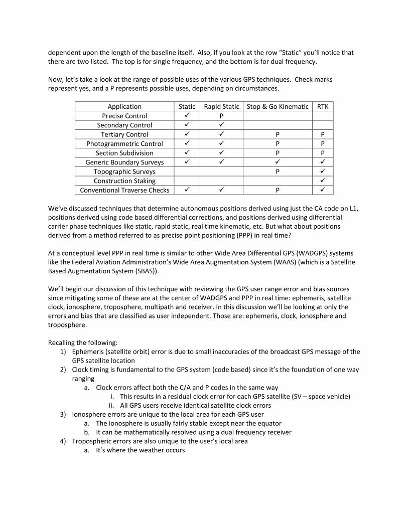
dependent upon the length of the baseline itself. Also, if you look at the row “Static” you’ll notice that there are two listed. The top is for single frequency, and the bottom is for dual frequency. Now, let’s take a look at the range of possible uses of the various GPS techniques. Check marks represent yes, and a P represents possible uses, depending on circumstances.

Application Static Rapid Static Stop & Go Kinematic RTK Precise Control P

Secondary Control Tertiary Control P P

Photogrammetric Control P P Section Subdivision P P

Generic Boundary Surveys Topographic Surveys P Construction Staking

Conventional Traverse Checks P We’ve discussed techniques that determine autonomous positions derived using just the CA code on L1, positions derived using code based differential corrections, and positions derived using differential carrier phase techniques like static, rapid static, real time kinematic, etc. But what about positions derived from a method referred to as precise point positioning (PPP) in real time? At a conceptual level PPP in real time is similar to other Wide Area Differential GPS (WADGPS) systems like the Federal Aviation Administration’s Wide Area Augmentation System (WAAS) (which is a Satellite Based Augmentation System (SBAS)). We’ll begin our discussion of this technique with reviewing the GPS user range error and bias sources since mitigating some of these are at the center of WADGPS and PPP in real time: ephemeris, satellite clock, ionosphere, troposphere, multipath and receiver. In this discussion we’ll be looking at only the errors and bias that are classified as user independent. Those are: ephemeris, clock, ionosphere and troposphere. Recalling the following:

1) Ephemeris (satellite orbit) error is due to small inaccuracies of the broadcast GPS message of the GPS satellite location

2) Clock timing is fundamental to the GPS system (code based) since it’s the foundation of one way ranging

a. Clock errors affect both the C/A and P codes in the same way i. This results in a residual clock error for each GPS satellite (SV – space vehicle)

ii. All GPS users receive identical satellite clock errors 3) Ionosphere errors are unique to the local area for each GPS user

a. The ionosphere is usually fairly stable except near the equator b. It can be mathematically resolved using a dual frequency receiver

4) Tropospheric errors are also unique to the user’s local area a. It’s where the weather occurs

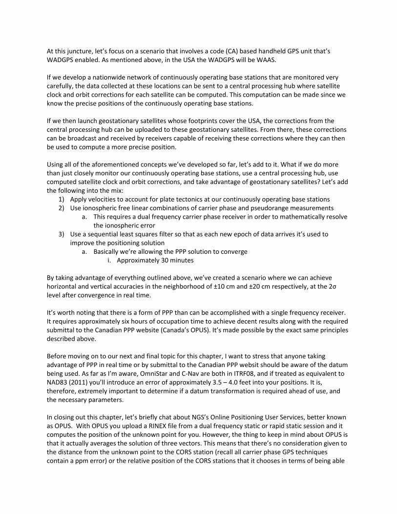
At this juncture, let’s focus on a scenario that involves a code (CA) based handheld GPS unit that’s WADGPS enabled. As mentioned above, in the USA the WADGPS will be WAAS. If we develop a nationwide network of continuously operating base stations that are monitored very carefully, the data collected at these locations can be sent to a central processing hub where satellite clock and orbit corrections for each satellite can be computed. This computation can be made since we know the precise positions of the continuously operating base stations. If we then launch geostationary satellites whose footprints cover the USA, the corrections from the central processing hub can be uploaded to these geostationary satellites. From there, these corrections can be broadcast and received by receivers capable of receiving these corrections where they can then be used to compute a more precise position. Using all of the aforementioned concepts we’ve developed so far, let’s add to it. What if we do more than just closely monitor our continuously operating base stations, use a central processing hub, use computed satellite clock and orbit corrections, and take advantage of geostationary satellites? Let’s add the following into the mix:

1) Apply velocities to account for plate tectonics at our continuously operating base stations 2) Use ionospheric free linear combinations of carrier phase and pseudorange measurements

a. This requires a dual frequency carrier phase receiver in order to mathematically resolve the ionospheric error

3) Use a sequential least squares filter so that as each new epoch of data arrives it’s used to improve the positioning solution

a. Basically we’re allowing the PPP solution to converge i. Approximately 30 minutes

By taking advantage of everything outlined above, we’ve created a scenario where we can achieve horizontal and vertical accuracies in the neighborhood of ±10 cm and ±20 cm respectively, at the 2σ level after convergence in real time. It’s worth noting that there is a form of PPP than can be accomplished with a single frequency receiver. It requires approximately six hours of occupation time to achieve decent results along with the required submittal to the Canadian PPP website (Canada’s OPUS). It’s made possible by the exact same principles described above. Before moving on to our next and final topic for this chapter, I want to stress that anyone taking advantage of PPP in real time or by submittal to the Canadian PPP websit should be aware of the datum being used. As far as I’m aware, OmniStar and C-Nav are both in ITRF08, and if treated as equivalent to NAD83 (2011) you’ll introduce an error of approximately 3.5 – 4.0 feet into your positions. It is, therefore, extremely important to determine if a datum transformation is required ahead of use, and the necessary parameters. In closing out this chapter, let’s briefly chat about NGS’s Online Positioning User Services, better known as OPUS. With OPUS you upload a RINEX file from a dual frequency static or rapid static session and it computes the position of the unknown point for you. However, the thing to keep in mind about OPUS is that it actually averages the solution of three vectors. This means that there’s no consideration given to the distance from the unknown point to the CORS station (recall all carrier phase GPS techniques contain a ppm error) or the relative position of the CORS stations that it chooses in terms of being able

to model the atmospheric conditions (troposphere) properly. While OPUS certainly has many uses, like a sanity check on your adjustment, the following procedures are recommended if you’re using your unknown point as control:

1) Choose CORS stations a. Surround unknown point; have at least four (if in cardinal directions) or more than four

if not in cardinal directions 2) Download all of the RINEX files for the appropriate date and time 3) Either bring all data into your own baseline processing program – e.g. GNSS solutions, TBC or

whatever program you may be using, or use the extended report from OPUS and extract the vectors from the extended report

a. Either way, you should pick your own stations 4) Process everything yourself (or use the baselines as processed by PAGES, obtained from the

OPUS extended report). Once you’re done processing, perform a least squares adjustments with your weighting based on a constant and ppm

By following this process you’re accounting for the distances from the CORS to your unknown position, and choosing geometry that’ll allow for better atmospheric modelling.

Chapter IV

GPS Modernization and GNSS As you may recall from Chapter 1, we presented a table with the different satellites that are part of GPS. It included the blocks with their respective launch periods, total number of satellites, and those still in orbit and healthy. In this chapter, we’ll cover the specific satellites that are part of the GPS modernization program, new codes that have been added since the original inception, and other satellite based systems that are part of what’s referred to as the Global Navigation Satellite System (GNSS). The first is Block IIR-M, with M meaning modernized replenishment; and Block IIF, with F meaning follow on. One of the things about both of these and Block IIR is that they all are backward compatible with Block II and Block IIA. One of the key components of the last 4 Block IIRs, all of the Block IIR-Ms, and all of the Block IIFs is that they have an improved antenna panel that allows for an increased GPS signal to be received by GPS receivers. In addition, additional frequencies were added to the Block IIR-Ms and Block IIFs underneath the GPS modernization program. There are two new civil codes on the L2 frequency called L2C-M and L2C-L. There are also two new military codes, known as M codes, one on L1 and one on L2. To satisfy aviation uses, a third civil code, on a new frequency, L5 was also added to Block IIF satellites. L5 has a broadcast frequency of 1,176.45MHz; and two new PRN codes modulated onto it, the I5 and Q5. One of the interesting things about the Q5 code is that it has no navigation data modulated onto it. The addition of the two new military codes really doesn’t do a lot for the average civilian user of GPS, however, the new civil codes will. With these, it’ll allow us to have better positioning accuracies since autonomous GPS code based receivers will be able to mathematically correct for the ionospheric effects and multipath will be mitigated. The L5, is of particular interest since it’ll be the most effective of all enhancements. It’s designed to be approximately five dB more powerful than L1, with a chipping rate of 10.23 Mcps versus 1.023 Mcps of L1. Based on its anticipated significant impacts, let’s look at some of its advantages:

1) Is anticipated to be available on 24 GPS satellites in 2021 2) Higher transmitted power than L1 or L2 3) Greater bandwidth for improved jamming resistance 4) Modern signal design (CNAV), including multiple message types 5) Bi-Phase Shift Key (BPSK) modulation 6) Includes dedicated channel for codeless tracking 7) Is broadcast in a radio band reserved exclusively for aviation safety services

a. It features higher power, greater bandwidth, and an advanced signal design 8) Will be used in combination with L1 and L2 to improve accuracy

a. Ionospheric correction i. Dual and triple frequency

b. Robustness i. Signal redundancy

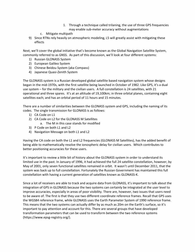
1. Through a technique called trilaning, the use of three GPS frequencies may enable sub-meter accuracy without augmentations

c. Mitigate multipath 9) Since RTNs rely heavily on atmospheric modeling, L5 will greatly assist with mitigating these

effects Next, we’ll cover the global initiative that’s become known as the Global Navigation Satellite System, commonly referred to as GNSS. As part of this discussion, we’ll look at four different systems:

1) Russian GLONASS System 2) European Galileo System 3) Chinese Beidou System (aka Compass) 4) Japanese Quasi-Zenith System

The GLONASS system is a Russian developed global satellite based navigation system whose designs began in the mid-1970s, with the first satellite being launched in October of 1982. Like GPS, it’s a dual use system – for the military and the civilian users. A full constellation is 24 satellites, with 21 operational and three spares. It’s at an altitude of 19,100km; in three orbital planes, containing eight satellites each; and has an orbital period of 11 hours and 15 minutes. There are a number of similarities between the GLONASS system and GPS, including the naming of its codes. The single transmission for GLONASS is as follows:

1) CA Code on L1 2) CA Code on L2 for the GLONASS M Satellites

a. The M in this case stands for modified 3) P Code on both L1 and L2 4) Navigation Message on both L1 and L2

Having the CA code on both the L1 and L2 frequencies (GLONASS M Satellites), has the added benefit of being able to mathematically resolve the ionospheric delay for civilian users. Which contributes to better positioning accuracies for these users. It’s important to review a little bit of history about the GLONASS system in order to understand its limited use in the past. In January of 1996, it had achieved the full 24 satellite constellation, however, by May of 2001, only seven functional satellites remained in orbit. It wasn’t until December 2011, that the system was back up to full constellation. Fortunately the Russian Government has maintained this full constellation with having a current generation of satellites known as GLONASS-K. Since a lot of receivers are able to track and acquire data from GLONASS, it’s important to talk about the integration of GPS in GLONASS because the two systems can certainly be integrated at the user level to improve accuracies, especially in areas of poor visibility. There are, however, two issues that users need to be aware of. The first is that they use two different coordinate reference frames. Recall that GPS uses the WGS84 reference frame, while GLONASS uses the Earth Parameter System of 1990 reference frame. This means that the two systems can actually differ by as much as 20m on the Earth’s surface, so it’s important to pay attention and account for this. There are several groups that have developed transformation parameters that can be used to transform between the two reference systems (https://www.epsg-registry.org/).

The second problem is that both systems use a different reference time. Now, this can be overcome by treating the time offset between the two systems as an additional variable in the receiver solution. Instead of having four satellites with four simultaneous equations, you have five satellites with five simultaneous equations. The next system to discuss, that’s part of the GNSS initiative, is the Galileo System. It’s the European developed, global satellite based navigation system that’s currently underway. Unlike GPS and GLONASS, it’s a civilian controlled satellite system, instead of government controlled, and is designed to deliver five types of services, outlined below:

1) Open Service (OS): a. Is free of charge b. Has a single frequency positioning accuracy at 95% confidence

i. Horizontal ± 15m ii. Vertical ± 30m

c. Has dual frequency positioning accuracy at 95% confidence i. Horizontal ±4m

ii. Vertical ±8M 2) Commercial Service (CS):

a. Fee based, therefore, restricted access b. Has dual frequency positioning accuracy at 95% confidence

i. Horizontal and Vertical less than ±1m 3) Safety of Live (SOL):

a. Is a global, open access system, designated as safety critical (maritime, rail transportation and aviation)

b. Has dual frequency positioning accuracy at 95% i. Horizontal and Vertical 4-8m

4) Public Regulation Service (PRS): a. Is restricted to approved government entities b. Has dual frequencies at 95% confidence

i. Horizontal ±6.5m ii. Vertical ±12m

5) Support to Search and Rescue (SAR): a. Has global access to aid in search and rescue efforts b. Has dual frequency position with accuracy at 95% confidence

i. Within a few meters Now, let’s look at a few specification of the Galileo system:

1) The full constellation consists of 30 Satellites; 27 operational and 3 spares 2) Satellites will be at an altitude of 23,222km 3) Satellites are in three orbital planes, containing 10 satellites each – 9 operational and one spare

in each orbital plane 4) The orbital period will be 14 hours, 4 minutes and 41 seconds 5) Each satellite will transmit six signals in three different bands

a. The six signals are: i. E1 OS, E1 PRS, E6 CS, E6 PRS, E5A and E5B

The datum and ellipsoid of Galileo are ETRS89 and GRS80, respectively. It’s aligned with ITRF89 and connected to the Eurasia plate.

The third system, that’s included as part of the GNSS initiative, is the Chinese Beidou system. The Beidou system is a regional, 2 dimensional positioning (vs. 3 dimensional) and navigation system. It provides regional coverage, between north latitudes of 5⁰ to 55⁰, and between east longitudes of 70⁰ to 140⁰. Unlike GPS, Galileo and GLONASS, Beidou is a two-way ranging system versus a one-way. At this time, there isn’t any real practical use of the Chinese Beidou system for individuals in North America (although Champion is attempting to track the satellites and make use of them); however, it is included in the GNSS initiative. The fourth and final system, that’s part of the GNSS initiative, is the Japanese Quasi-Zenith Satellite System (QZSS). It’s a regional satellite navigation system that’s GPS compatible and serves all of Japan and Asia. The constellation consists of three satellites in total, one in three different geosynchronous orbits. They have an altitude of approximately 35,786 km and, like Beidou, it doesn’t appear to have any practical use in North America. If we focus in on just the three of the five systems that have direct impact on North America: GPS, GLONASS and Galileo, and discard Beidou and Japanese Quasi-Zenith systems, what can we expect in North America?

1) We’ll see more satellites 2) We’ll have greater accessibility among trees and urban canyons 3) More flexibility 4) Greater reliability 5) Faster positioning 6) Faster initialization for carrier phase receivers 7) Multipath mitigation 8) And ultimately, better accuracies all around

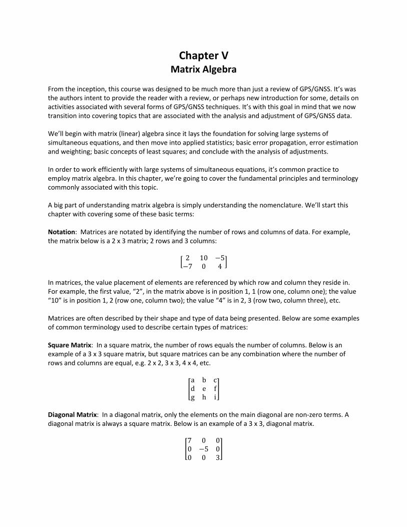
Chapter V Matrix Algebra

From the inception, this course was designed to be much more than just a review of GPS/GNSS. It’s was the authors intent to provide the reader with a review, or perhaps new introduction for some, details on activities associated with several forms of GPS/GNSS techniques. It’s with this goal in mind that we now transition into covering topics that are associated with the analysis and adjustment of GPS/GNSS data. We’ll begin with matrix (linear) algebra since it lays the foundation for solving large systems of simultaneous equations, and then move into applied statistics; basic error propagation, error estimation and weighting; basic concepts of least squares; and conclude with the analysis of adjustments. In order to work efficiently with large systems of simultaneous equations, it’s common practice to employ matrix algebra. In this chapter, we’re going to cover the fundamental principles and terminology commonly associated with this topic. A big part of understanding matrix algebra is simply understanding the nomenclature. We’ll start this chapter with covering some of these basic terms: Notation: Matrices are notated by identifying the number of rows and columns of data. For example, the matrix below is a 2 x 3 matrix; 2 rows and 3 columns:

� 2 10 −5−7 0 4 �

In matrices, the value placement of elements are referenced by which row and column they reside in. For example, the first value, “2”, in the matrix above is in position 1, 1 (row one, column one); the value “10” is in position 1, 2 (row one, column two); the value “4” is in 2, 3 (row two, column three), etc. Matrices are often described by their shape and type of data being presented. Below are some examples of common terminology used to describe certain types of matrices: Square Matrix: In a square matrix, the number of rows equals the number of columns. Below is an example of a 3 x 3 square matrix, but square matrices can be any combination where the number of rows and columns are equal, e.g. 2 x 2, 3 x 3, 4 x 4, etc.

�a b cd e fg h i

�

Diagonal Matrix: In a diagonal matrix, only the elements on the main diagonal are non-zero terms. A diagonal matrix is always a square matrix. Below is an example of a 3 x 3, diagonal matrix.

�7 0 00 −5 00 0 3

�

Transposed Matrix: One of the more common functions that we need to be able to perform is transposing a matrix. This is a fairly simple process since you’re just flipping the row and column numbers. Below is an example where a 2 x 3 matrix, reference as “A”, is transposed to a 3 x 2 matrix, AT:

A = �2 4 75 3 1�

AT = �2 54 37 1

�

In this scenario, the position of the values of the data set get transposed:

A AT Row, Column Row, Colum 1, 1 1,1 1, 2 2,1 1, 3 3,1 2, 1 1,2 2, 2 2,2 2, 3 3, 2

Basic Mathematical Functions with Matrices Adding & Subtracting: Another basic mathematical function we need to review is adding and subtracting matrices. In order to add or subtract matrices, it’s important to recall that they must be the same size. In the first example below, we’re adding the matrices, where A + B = C. A and B matrices are the same size, where each value in one matrix has a corresponding value in the next matrix. In this example, both are 2 x 3, therefore, the result is also the same size, a 2 x 3 matrix. You add/subtract the corresponding values based on their location in the matrices; so 1,1 in A is added to value 1,1 in B, resulting in 1,1 in the resulting matrix C.

Numerical Example of Addition of Matrices (A + B = C):

�7 3 −12 −5 6 � + � 1 5 6

−4 −2 3� = � 8 8 5−2 −7 9�

Numerical Example of Subtraction of Matrices (A – B = C):

�7 3 −12 −5 6 � - � 1 5 6

−4 −2 3� = �6 −2 −76 −3 3 �

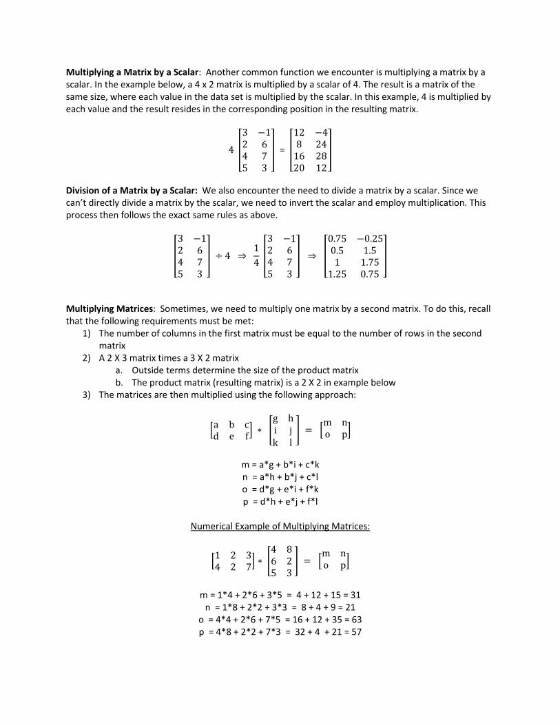
Multiplying a Matrix by a Scalar: Another common function we encounter is multiplying a matrix by a scalar. In the example below, a 4 x 2 matrix is multiplied by a scalar of 4. The result is a matrix of the same size, where each value in the data set is multiplied by the scalar. In this example, 4 is multiplied by each value and the result resides in the corresponding position in the resulting matrix.

4 �

3 −12 64 75 3

� = �

12 −48 24

16 2820 12

�

Division of a Matrix by a Scalar: We also encounter the need to divide a matrix by a scalar. Since we can’t directly divide a matrix by the scalar, we need to invert the scalar and employ multiplication. This process then follows the exact same rules as above.

�

3 −12 64 75 3

� ÷ 4 ⇒ 14

�

3 −12 64 75 3

� ⇒ �

0.75 −0.250.5 1.51 1.75

1.25 0.75

�

Multiplying Matrices: Sometimes, we need to multiply one matrix by a second matrix. To do this, recall that the following requirements must be met:

1) The number of columns in the first matrix must be equal to the number of rows in the second matrix

2) A 2 X 3 matrix times a 3 X 2 matrix a. Outside terms determine the size of the product matrix b. The product matrix (resulting matrix) is a 2 X 2 in example below

3) The matrices are then multiplied using the following approach:

�a b cd e f� ∗ �

g hi jk l

� = �m no p�

m = a*g + b*i + c*k n = a*h + b*j + c*l o = d*g + e*i + f*k p = d*h + e*j + f*l

Numerical Example of Multiplying Matrices:

�1 2 34 2 7� ∗ �

4 86 25 3

� = �m no p�

m = 1*4 + 2*6 + 3*5 = 4 + 12 + 15 = 31

n = 1*8 + 2*2 + 3*3 = 8 + 4 + 9 = 21 o = 4*4 + 2*6 + 7*5 = 16 + 12 + 35 = 63 p = 4*8 + 2*2 + 7*3 = 32 + 4 + 21 = 57

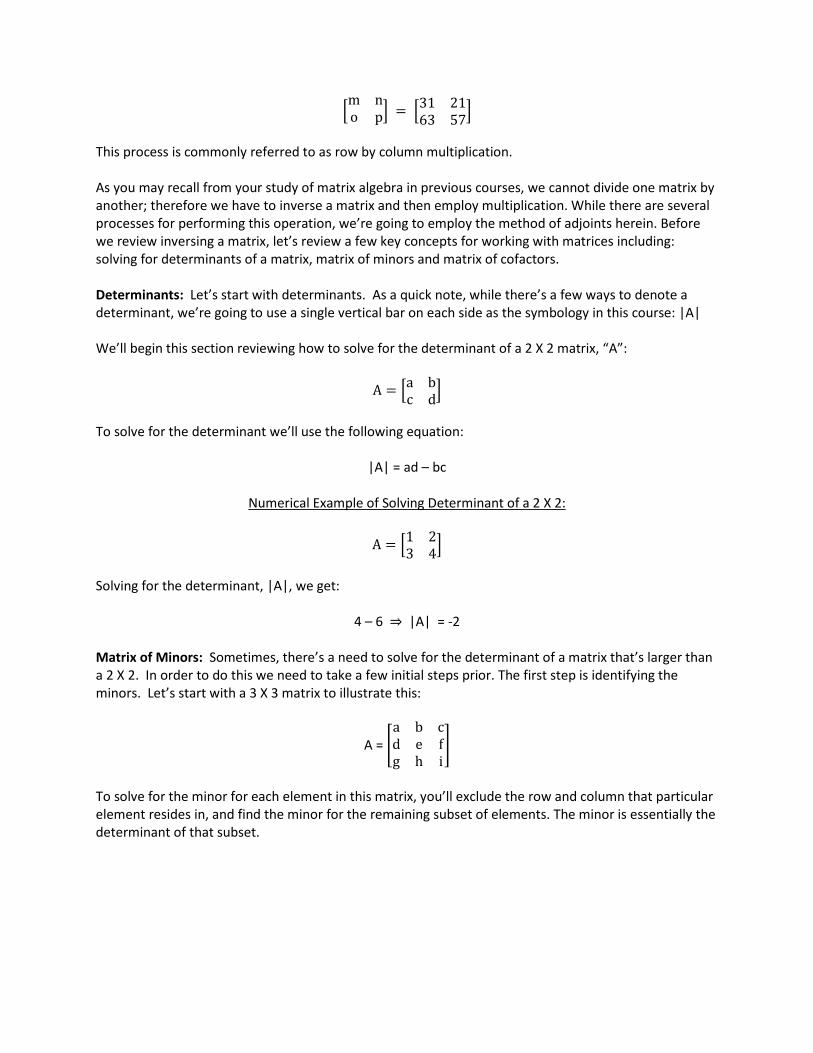
�m no p� = �31 21

63 57�

This process is commonly referred to as row by column multiplication. As you may recall from your study of matrix algebra in previous courses, we cannot divide one matrix by another; therefore we have to inverse a matrix and then employ multiplication. While there are several processes for performing this operation, we’re going to employ the method of adjoints herein. Before we review inversing a matrix, let’s review a few key concepts for working with matrices including: solving for determinants of a matrix, matrix of minors and matrix of cofactors. Determinants: Let’s start with determinants. As a quick note, while there’s a few ways to denote a determinant, we’re going to use a single vertical bar on each side as the symbology in this course: |A| We’ll begin this section reviewing how to solve for the determinant of a 2 X 2 matrix, “A”:

A = �a bc d�

To solve for the determinant we’ll use the following equation:

|A| = ad – bc

Numerical Example of Solving Determinant of a 2 X 2:

A = �1 23 4�

Solving for the determinant, |A|, we get:

4 – 6 ⇒ |A| = -2 Matrix of Minors: Sometimes, there’s a need to solve for the determinant of a matrix that’s larger than a 2 X 2. In order to do this we need to take a few initial steps prior. The first step is identifying the minors. Let’s start with a 3 X 3 matrix to illustrate this:

A = �a b cd e fg h i

�

To solve for the minor for each element in this matrix, you’ll exclude the row and column that particular element resides in, and find the minor for the remaining subset of elements. The minor is essentially the determinant of that subset.

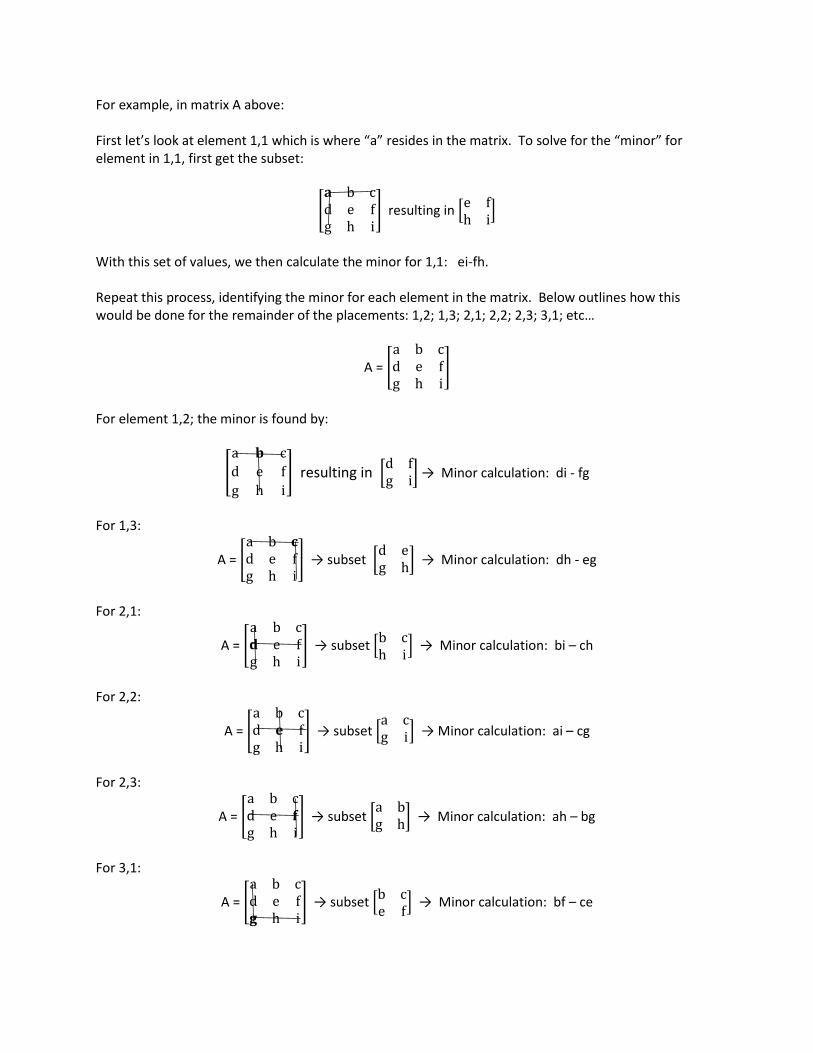
For example, in matrix A above: First let’s look at element 1,1 which is where “a” resides in the matrix. To solve for the “minor” for element in 1,1, first get the subset:

�𝐚𝐚 b cd e fg h i

� resulting in �e fh i�

With this set of values, we then calculate the minor for 1,1: ei-fh. Repeat this process, identifying the minor for each element in the matrix. Below outlines how this would be done for the remainder of the placements: 1,2; 1,3; 2,1; 2,2; 2,3; 3,1; etc…

A = �a b cd e fg h i

�

For element 1,2; the minor is found by:

�a 𝐛𝐛 cd e fg h i

� resulting in �d fg i� → Minor calculation: di - fg

For 1,3:

A = �a b 𝐜𝐜d e fg h i

� → subset �d eg h� → Minor calculation: dh - eg

For 2,1:

A = �a b c𝐝𝐝 e fg h i

� → subset �b ch i� → Minor calculation: bi – ch

For 2,2:

A = �a b cd 𝐞𝐞 fg h i

� → subset �a cg i� → Minor calculation: ai – cg

For 2,3:

A = �a b cd e 𝐟𝐟g h i

� → subset �a bg h� → Minor calculation: ah – bg

For 3,1:

A = �a b cd e f𝐠𝐠 h i

� → subset �b ce f� → Minor calculation: bf – ce

For 3,2:

A = �a b cd e fg 𝐡𝐡 i

� → subset �a cd f� → Minor calculation: af – cd

For 3,3:

A = �a b cd e fg h 𝐢𝐢

� → subset �a bd e� → Minor calculation: ae – bd

Example for Matrix of Minors:

A = �4 3 23 4 12 3 4

�

Resulting minors for each element, respectively will be:

1,1 = 16-3 ⇒ 13 1,2 = 12-2 ⇒ 10 1,3 = 9-8 ⇒ 1 2,1 = 12-6 ⇒ 6

2,2 = 16-4 ⇒ 12 2,3 = 12-6 ⇒ 6 3,1 = 3-8 ⇒ -5 3,2 = 4-6 ⇒ -2 3,3 = 16-9 ⇒ 7

Once the minors have been determined, then create a matrix of minors. Each minor is placed in its corresponding position. Below is the resulting matrix of minors from the above example:

A = �13 10 16 12 6

−5 −2 7�

Matrix of Cofactors: Once we’ve determined the matrix of minors, the next step is to determine a matrix of cofactors. We do this by determining cofactors for each element in the matrix of minors. The first thing to recall is that cofactors follow certain rules:

1) If the row + column is even the sign of the resulting cofactor is the same as for the minor 2) If the row + column is odd, the sign of the cofactors is the opposite as for the minor

Using our 3 X 3 matrix of minors, the resulting matrix of cofactors will be as follows based on following the aforementioned rules:

1 + 1 = 2 (even) 1 + 2 = 3 (odd) 1 + 3 = 4 (even)

2 + 1 = 3 (odd) 2 + 2 = 4 (even) 2 + 3 = 5 (odd) 3 + 1 = 4 (even) 3 + 2 = 5 (odd) 3 + 3 = 6 (even)

Matrix of Cofactors:

The matrix of cofactors, derived from matrix of minors = �13 −10 1−6 12 −6−5 2 7

�

Determinants for Matrices Larger than 2 X 2: To finish our discussion on determinants, we need to come full circle and review briefly now how to solve for determinants for matrices larger than a 2 X 2. Let’s begin with the 3 X 3 matrix, “A”: Select any row or column (but not a diagonal) in this matrix. Remember, when selecting the row or column, it can be very advantageous to select one with as many zero values as possible, as this will simplify the work Once selected, we’ll be employing cofactors, derived from minors as discussed above. Starting with our 3 X 3 matrix:

A = �a b cd e fg h i

�

We’ll use row one (a, b & c) and use the following formula for solving for our determinant for a 3 X 3 matrix:

|A| = a (ei – fh) – b (di – fg) + c (dh – eg)

Numerical Example of Solving for Determinant of a 3 X 3 Matrix:

A = �4 3 23 4 12 3 4

�

Using row one, and the formula noted above, we’ll solve for the determinant, |A|:

|A| = 4 (16-3) – 3 (12-2) + 2 (9-8) ⇒ |A| = 4 (13) – 3 (10) + 2 (1) ⇒

|A| = 24 Generally, we’ll have the advantage of doing this with software or a calculator, but understanding this long handed methodology, at least with a 3 X 3 matrix gives a sense for how the determinant is derived with larger data sets.

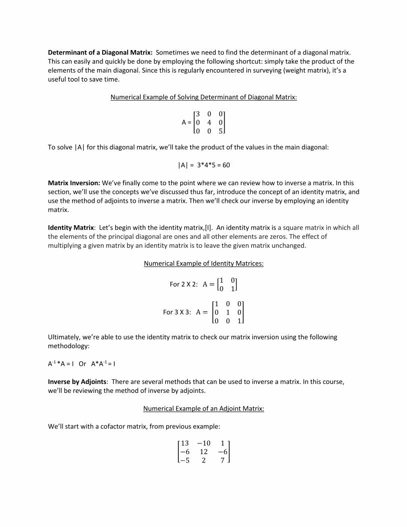
Determinant of a Diagonal Matrix: Sometimes we need to find the determinant of a diagonal matrix. This can easily and quickly be done by employing the following shortcut: simply take the product of the elements of the main diagonal. Since this is regularly encountered in surveying (weight matrix), it’s a useful tool to save time.

Numerical Example of Solving Determinant of Diagonal Matrix:

A = �3 0 00 4 00 0 5

�

To solve |A| for this diagonal matrix, we’ll take the product of the values in the main diagonal:

|A| = 3*4*5 = 60 Matrix Inversion: We’ve finally come to the point where we can review how to inverse a matrix. In this section, we’ll use the concepts we’ve discussed thus far, introduce the concept of an identity matrix, and use the method of adjoints to inverse a matrix. Then we’ll check our inverse by employing an identity matrix. Identity Matrix: Let’s begin with the identity matrix,[I]. An identity matrix is a square matrix in which all the elements of the principal diagonal are ones and all other elements are zeros. The effect of multiplying a given matrix by an identity matrix is to leave the given matrix unchanged.

Numerical Example of Identity Matrices:

For 2 X 2: A = �1 00 1�

For 3 X 3: A = �1 0 00 1 00 0 1

�

Ultimately, we’re able to use the identity matrix to check our matrix inversion using the following methodology: A-1 *A = I Or A*A-1 = I

Inverse by Adjoints: There are several methods that can be used to inverse a matrix. In this course, we’ll be reviewing the method of inverse by adjoints.

Numerical Example of an Adjoint Matrix:

We’ll start with a cofactor matrix, from previous example:

�13 −10 1−6 12 −6−5 2 7

�

The adjoint matrix is found by transposing the cofactor matrix:

�13 −6 −5

−10 12 21 −6 7

�

Now, that we’ve solved for the adjoint matrix and the determinant of the matrix, we can use the following formula for inverting the matrix:

A-1 = Adjoint of A

|A|

From the previous example, our determinant, |A| = 24. Using the inversion formula and the adjoint matrix we just derived, we get the following inverted matrix, A1:

A-1 = 1/24 * �13 −6 −5

−10 12 21 −6 7

�

Now, we’ll reduce the fractions in the matrix, respectively:

A-1 =

⎣⎢⎢⎡

1324� −1

4� −524�

−512� 1

2� 112�

124� −1

4� 724� ⎦

⎥⎥⎤

As mentioned earlier, we can check the inverse using A * A-1 = I

�4 3 23 4 12 3 4

� X

⎣⎢⎢⎡

1324� −1

4� −524�

−512� 1

2� 112�

124� −1

4� 724� ⎦

⎥⎥⎤ ⇒

1, 1 = (4) (13/24) + (3) (-5/12) + (2) (1/24) => 1

1, 2 = (4) (-1/4) + (3) (1/2) + (2) (-1/4) => 0 1, 3 = (4) (-5/24) + (3) (1/12) + (2) (7/24) => 0

2, 1 = (3) (13/24) + (4) (-5/12) + (1) (1/24) => 0 2, 2 = (3) (-1/4) + (4) (1/2) + (1) (-1/4) => 1

2, 3 = (3) (-5/24) + (4) (1/12) + (1) (7/24) => 0 3, 1 = (2) (13/24) + (3) (-5/12) + (4) (1/24) => 0

3, 2 = (2) (-1/4) + (3) (1/2) + (4) (-1/4) => 0 3, 3 = (2) (-5/24) + (3) (1/12) + (4) (7/24) => 1

The resulting identity matrix confirms we have accurately inverted the matrix:

I = �1 0 00 1 00 0 1

�

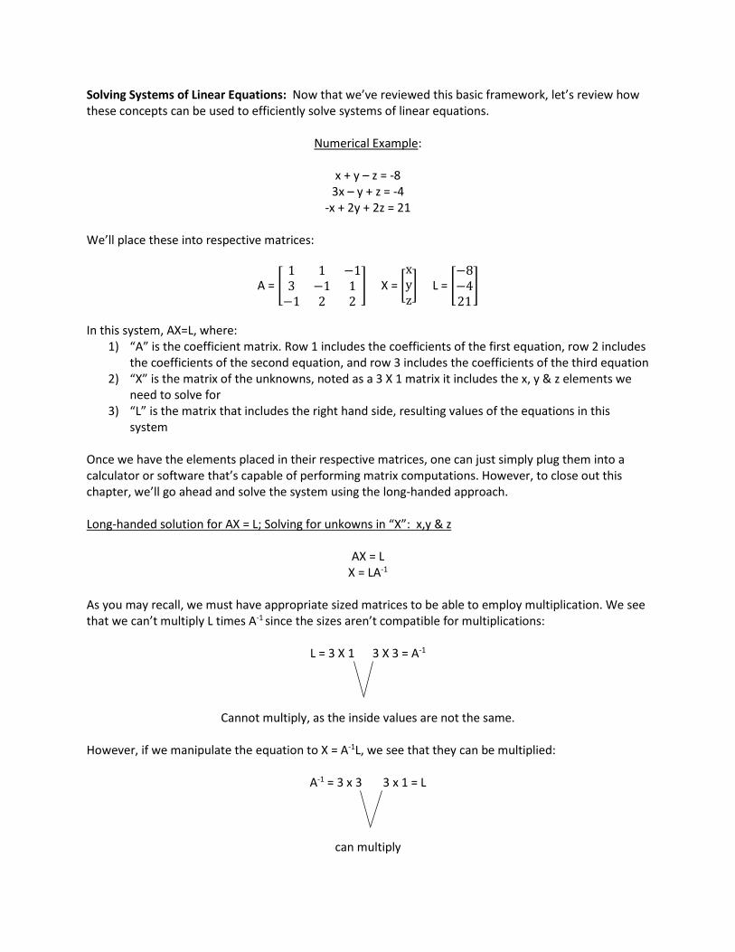
Solving Systems of Linear Equations: Now that we’ve reviewed this basic framework, let’s review how these concepts can be used to efficiently solve systems of linear equations.

Numerical Example:

x + y – z = -8 3x – y + z = -4

-x + 2y + 2z = 21 We’ll place these into respective matrices:

A = �1 1 −13 −1 1

−1 2 2� X = �

xyz

� L = �−8−421

�

In this system, AX=L, where:

1) “A” is the coefficient matrix. Row 1 includes the coefficients of the first equation, row 2 includes the coefficients of the second equation, and row 3 includes the coefficients of the third equation

2) “X” is the matrix of the unknowns, noted as a 3 X 1 matrix it includes the x, y & z elements we need to solve for

3) “L” is the matrix that includes the right hand side, resulting values of the equations in this system

Once we have the elements placed in their respective matrices, one can just simply plug them into a calculator or software that’s capable of performing matrix computations. However, to close out this chapter, we’ll go ahead and solve the system using the long-handed approach. Long-handed solution for AX = L; Solving for unkowns in “X”: x,y & z

AX = L X = LA-1

As you may recall, we must have appropriate sized matrices to be able to employ multiplication. We see that we can’t multiply L times A-1 since the sizes aren’t compatible for multiplications:

L = 3 X 1 3 X 3 = A-1

Cannot multiply, as the inside values are not the same. However, if we manipulate the equation to X = A-1L, we see that they can be multiplied:

A-1 = 3 x 3 3 x 1 = L

can multiply

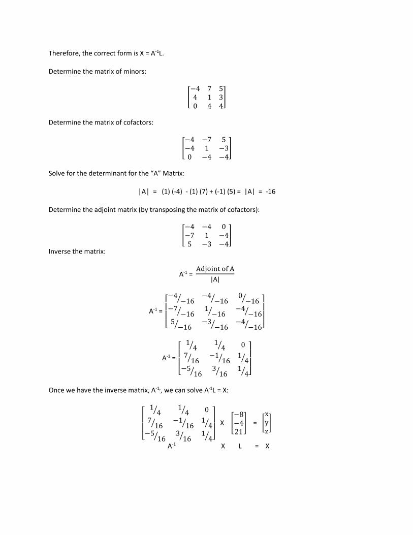
Therefore, the correct form is X = A-1L. Determine the matrix of minors:

�−4 7 54 1 30 4 4

�

Determine the matrix of cofactors:

�−4 −7 5−4 1 −30 −4 −4

�

Solve for the determinant for the “A” Matrix:

│A│ = (1) (-4) - (1) (7) + (-1) (5) = |A| = -16 Determine the adjoint matrix (by transposing the matrix of cofactors):

�−4 −4 0−7 1 −45 −3 −4

�

Inverse the matrix:

A-1 = Adjoint of A

|A|

A-1 =

⎣⎢⎢⎡−4

−16� −4−16� 0

−16�−7

−16� 1−16� −4

−16�5

−16� −3−16� −4

−16� ⎦⎥⎥⎤

A-1 =

⎣⎢⎢⎡

14� 1

4� 07

16� −116� 1

4�−5

16� 316� 1

4� ⎦⎥⎥⎤

Once we have the inverse matrix, A-1,, we can solve A-1L = X:

⎣⎢⎢⎡

14� 1

4� 07

16� −116� 1

4�−5

16� 316� 1

4� ⎦⎥⎥⎤

X �−8−421

� = �xyz

�

A-1 X L = X

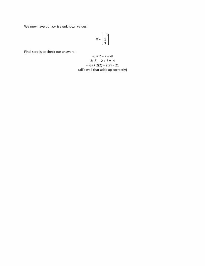
We now have our x,y & z unknown values:

X = �−327

�

Final step is to check our answers:

-3 + 2 – 7 = -8 3(-3) – 2 + 7 = -4

-(-3) + 2(2) + 2(7) = 21 (all’s well that adds up correctly)

Chapter VI Applied Statistics

Now that we’ve completed our review of matrix algebra we need to review statistics from an applied perspective. The material covered in this chapter lays the foundation for understanding weighting and for properly analyzing the results generated from a least squares adjustment. The material will be presented through a combination of definitions, mathematical equations, and mathematical examples. Population: all possible measurements that could be made. Generally infinite and unknown. Sample: a subset of data from the population. What we work with in surveying. Arithmetic Mean (Average): denoted by 𝑋𝑋:

𝑋𝑋 = 𝛴𝛴𝑥𝑥𝑖𝑖

𝑛𝑛

Where ∑Xi = the summation of each individual measurement

n = the total number of measurements

Numerical Example of Calculating an Arithmetic Mean:

Measurements: x1 = 10.5 x2 = 10.4 x3 = 10.3 x4 = 10.4

n = 4

𝑋𝑋 = 10.5 + 10.4 + 10.3 + 10.4

4= 10.4

Residual: the difference between the adjusted value and the measured value, or the amount a measurement adjusted. Residual, for purposes of this course, will be denoted by v.

Numerical Example of Residual:

Using the data from the previous example, the adjusted value would be 10.4. Therefore, the residuals would be:

v1 = 10.4 - 10.5 = -0.1 v2 = 10.4 - 10.4 = 0.0 v3 = 10.4 - 10.3 = 0.1 v4 = 10.4 -10.4 = 0.0

Variance: measures the precision of the dataset. In this course, we’ll denote variance as S2.

S2 = (Σv2 )𝑛𝑛 − 1

Where Ʃv2 = the summation of the residuals squared n = as previously defined

Numerical Example of a Variance:

Using the data from the previous examples:

𝑆𝑆2 = −0.12 + 0.02 + 0.12 + 0.02

4 − 1= 0.0067

Standard Deviation: is the square root of the variance and is used to draw conclusions about probability. It will be denoted by S:

𝑆𝑆 = �𝑆𝑆2 = � Σv2

𝑛𝑛 − 1

Numerical Example of a Standard Deviation: Using the data from the variance example, the standard deviation is:

√0.0067 = ±0.08′

So what does the ±0.08 actually mean? By creating a confidence interval using the mean and standard deviation, 𝑋𝑋 ±S (10.4 -0.08 and 10.4 + 0.08) you can state that 68% of the time, a measurement will fall between 10.32 and 10.48 But in surveying we don’t normally want to be 68% statistically correct, therefore, we use multipliers to increase our confidence interval.

50% = 0.6745 * S 90% = 1.6449 * S 95% = 1.96 * S normally referred to as 2 sigma (acceptance) 99.7% = 2.965 * S normally referred to as 3 sigma (rejection) 99.9% = 3.29 * S

In surveying we tend to use 2σ and 3σ. The confidence interval for 2σ would be: 10.24 to 10.56.

It’s important to recognize that the smaller the standard deviation is, the more precise your measurements are. For example:

S = ±0.01 versus S = ±0.1

If the mean = 10.00

9.99 - 10.01 versus 9.90 - 10.10

Standard Error in the Mean: The standard error in the mean reflects the uncertainty in the mean as opposed to a single observation.

𝑆𝑆𝑆𝑆𝑆𝑆 =𝑆𝑆

√𝑛𝑛

The applied meaning of the standard error in the mean is as follows: if you made the same number of observations, under the same conditions, with the same equipment, you would be approximately 68% (one sigma) confident that you would fall within the range defined by the mean and plus or minus the standard error in the mean. Normalized Residuals:

SvNR ||

=

Estimate Error|| vNR =

Numerical Examples of Normalized Residuals:

Example 1: v = -0.03 and S = 0.09

𝑁𝑁𝑁𝑁 = 0.030.09

= 0.33

Example 2: v = 0.10 and S = 0.03

𝑁𝑁𝑁𝑁 = 0.100.03

= 3.3

Example 1 would indicate that your error estimate is too pessimistic. You did better work than you thought. Example 2 would indicate that your error estimate is too optimistic. Your work was not as good as you thought or you have a potential blunder. Normalized residuals are also known as Standardized Residuals; Snoop Numbers and Snoop Values

Root Mean Square (RMS): can be thought of as an average residual

𝑁𝑁𝑆𝑆𝑆𝑆 = �∑ 𝑣𝑣2

𝑛𝑛

∑ 𝑣𝑣2 = summation of the residuals squared

n = number of measurements

Note: RTK GPS gives you RMS values in real time and are used as one method of evaluating the quality of your coordinates in the field. Degrees of Freedom: The number of measurements beyond what’s needed to solve for a unique solution. Number of measurements – number of unknowns

1) This raises the question, what’s the difference between redundancy and degrees of freedom?

a. Turning 4 sets of angles (D & R) i. Is this eight angles, four angles or one angle with an estimated error associated

with it? 1. Redundancy – one average value with an estimated error

b. What if we break the set up and turn 4 more sets of angles (D & R)? i. Is this redundancy or degrees of freedom?

1. Degrees of Freedom Degrees of Freedom – For a GPS Network: DF = 3 (the number of control stations) + 3 (the number of vectors) – 3 (the total number of stations)

Numerical Example of Degrees of Freedom for a GPS network:

Vector from A to B Vector from B to C Vector from C to D Vector from D to A Vector from A to C Vector from B to D

Control station A is held fixed

Solution: DF = 3 (the number of control stations) + 3 (the number of vectors) – 3 (the total number of stations) => 3(1) + 3(6) – 3(4) = 3 + 18 – 12 = 9 Degrees of Freedom

Standard Error of Unit Weight:

Standard Error of Unit Weight = �∑ 𝑤𝑤𝑣𝑣2

𝐷𝐷𝐷𝐷

Ʃ = summation w = weight v2 = residuals squared DF = Degrees of Freedom Note 1: Normalized residuals are an indication of your weighting for a single measurement, while the standard error of unit weight is an indication of your weighting for the entire network. Note 2: If your weighting was perfect, your normalized residuals and standard error of unit weight would equal one.

Standard Error of Unit Weight using Matrix Notation = DF

wvvTΣ

vT = residual matrix transposed v = residual matrix DF = Degrees of Freedom w = weight matrix Chi Squared Test: the standard error of unit weight is statistically evaluated using the chi squared test. This test is predicated on degrees of freedom. That is, the closer your sample data set gets to the population (the more degrees of freedom you have), the less variability you will have in your statistical indicators. In order to pass, your standard error of unit weight must fall within your chi squared range.

1) The Chi squared test answers the following question:

a. Do the residuals (v) reflect my error estimations based on the resultant standard error of unit weight?

2) The Chi squared test is normally performed at the 95% confidence level in what is termed a two tailed test

3) The two tailed test means that the standard error of unit weight could be too high or too low

Upper-tail critical values of chi-square distribution with n degrees of freedom (What’s circled in red will be used in a numerical example)

DF 0.90 0.95 0.975 0.99 0.999 1 2.706 3.841 5.024 6.635 10.828 2 4.605 5.991 7.378 9.210 13.816 3 6.251 7.815 9.348 11.345 16.266 4 7.779 9.488 11.143 13.277 18.467 5 9.236 11.070 12.833 15.086 20.515 6 10.645 12.592 14.449 16.812 22.458 7 12.017 14.067 16.013 18.475 24.322 8 13.362 15.507 17.535 20.090 26.125

9 14.684 16.919 19.023 21.666 27.877 10 15.987 18.307 20.483 23.209 29.588 11 17.275 19.675 21.920 24.725 31.264 12 18.549 21.026 23.337 26.217 32.910 13 19.812 22.362 24.736 27.688 34.528 14 21.064 23.685 26.119 29.141 36.123 15 22.307 24.996 27.488 30.578 37.697 16 23.542 26.296 28.845 32.000 39.252 17 24.769 27.587 30.191 33.409 40.790 18 25.989 28.869 31.526 34.805 42.312 19 27.204 30.144 32.852 36.191 43.820 20 28.412 31.410 34.170 37.566 45.315 21 29.615 32.671 35.479 38.932 46.797 22 30.813 33.924 36.781 40.289 48.268 23 32.007 35.172 38.076 41.638 49.728 24 33.196 36.415 39.364 42.980 51.179 25 34.382 37.652 40.646 44.314 52.620 26 35.563 38.885 41.923 45.642 54.052 27 36.741 40.113 43.195 46.963 55.476 28 37.916 41.337 44.461 48.278 56.892 29 39.087 42.557 45.722 49.588 58.301 30 40.256 43.773 46.979 50.892 59.703 31 41.422 44.985 48.232 52.191 61.098 32 42.585 46.194 49.480 53.486 62.487 33 43.745 47.400 50.725 54.776 63.870 34 44.903 48.602 51.966 56.061 65.247 35 46.059 49.802 53.203 57.342 66.619 36 47.212 50.998 54.437 58.619 67.985 37 48.363 52.192 55.668 59.893 69.347 38 49.513 53.384 56.896 61.162 70.703 39 50.660 54.572 58.120 62.428 72.055 40 51.805 55.758 59.342 63.691 73.402 41 52.949 56.942 60.561 64.950 74.745 42 54.090 58.124 61.777 66.206 76.084 43 55.230 59.304 62.990 67.459 77.419 44 56.369 60.481 64.201 68.710 78.750 45 57.505 61.656 65.410 69.957 80.077 46 58.641 62.830 66.617 71.201 81.400 47 59.774 64.001 67.821 72.443 82.720 48 60.907 65.171 69.023 73.683 84.037 49 62.038 66.339 70.222 74.919 85.351 50 63.167 67.505 71.420 76.154 86.661 51 64.295 68.669 72.616 77.386 87.968 52 65.422 69.832 73.810 78.616 89.272 53 66.548 70.993 75.002 79.843 90.573 54 67.673 72.153 76.192 81.069 91.872

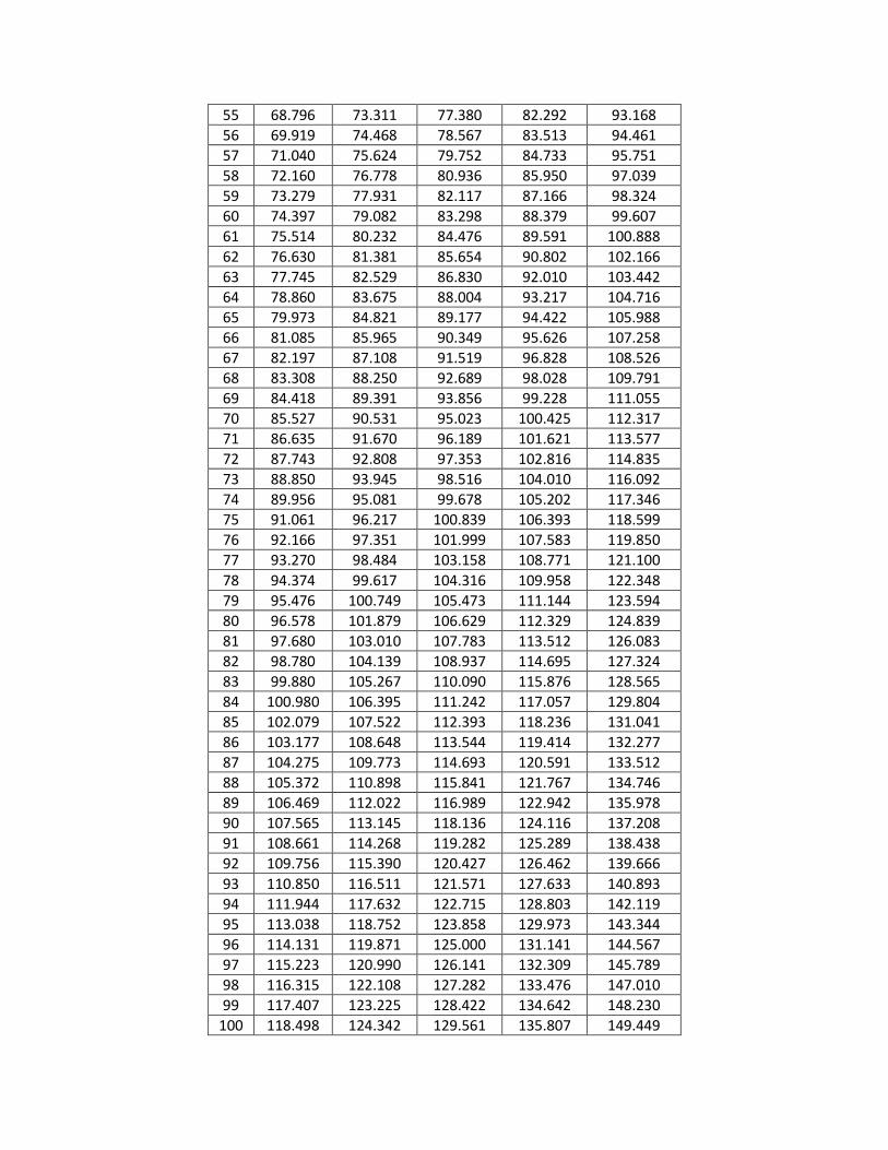
55 68.796 73.311 77.380 82.292 93.168 56 69.919 74.468 78.567 83.513 94.461 57 71.040 75.624 79.752 84.733 95.751 58 72.160 76.778 80.936 85.950 97.039 59 73.279 77.931 82.117 87.166 98.324 60 74.397 79.082 83.298 88.379 99.607 61 75.514 80.232 84.476 89.591 100.888 62 76.630 81.381 85.654 90.802 102.166 63 77.745 82.529 86.830 92.010 103.442 64 78.860 83.675 88.004 93.217 104.716 65 79.973 84.821 89.177 94.422 105.988 66 81.085 85.965 90.349 95.626 107.258 67 82.197 87.108 91.519 96.828 108.526 68 83.308 88.250 92.689 98.028 109.791 69 84.418 89.391 93.856 99.228 111.055 70 85.527 90.531 95.023 100.425 112.317 71 86.635 91.670 96.189 101.621 113.577 72 87.743 92.808 97.353 102.816 114.835 73 88.850 93.945 98.516 104.010 116.092 74 89.956 95.081 99.678 105.202 117.346 75 91.061 96.217 100.839 106.393 118.599 76 92.166 97.351 101.999 107.583 119.850 77 93.270 98.484 103.158 108.771 121.100 78 94.374 99.617 104.316 109.958 122.348 79 95.476 100.749 105.473 111.144 123.594 80 96.578 101.879 106.629 112.329 124.839 81 97.680 103.010 107.783 113.512 126.083 82 98.780 104.139 108.937 114.695 127.324 83 99.880 105.267 110.090 115.876 128.565 84 100.980 106.395 111.242 117.057 129.804 85 102.079 107.522 112.393 118.236 131.041 86 103.177 108.648 113.544 119.414 132.277 87 104.275 109.773 114.693 120.591 133.512 88 105.372 110.898 115.841 121.767 134.746 89 106.469 112.022 116.989 122.942 135.978 90 107.565 113.145 118.136 124.116 137.208 91 108.661 114.268 119.282 125.289 138.438 92 109.756 115.390 120.427 126.462 139.666 93 110.850 116.511 121.571 127.633 140.893 94 111.944 117.632 122.715 128.803 142.119 95 113.038 118.752 123.858 129.973 143.344 96 114.131 119.871 125.000 131.141 144.567 97 115.223 120.990 126.141 132.309 145.789 98 116.315 122.108 127.282 133.476 147.010 99 117.407 123.225 128.422 134.642 148.230

100 118.498 124.342 129.561 135.807 149.449

Lower-tail critical values of chi-square distribution with n degrees of freedom (What’s circled in red will be used in a numerical example)

DF 0.10 0.05 0.025 0.01 0.001 1 .016 .004 .001 .000 .000 2 .211 .103 .051 .020 .002 3 .584 .352 .216 .115 .024 4 1.064 .711 .484 .297 .091 5 1.610 1.145 .831 .554 .210 6 2.204 1.635 1.237 .872 .381 7 2.833 2.167 1.690 1.239 .598 8 3.490 2.733 2.180 1.646 .857 9 4.168 3.325 2.700 2.088 1.152

10 4.865 3.940 3.247 2.558 1.479 11 5.578 4.575 3.816 3.053 1.834 12 6.304 5.226 4.404 3.571 2.214 13 7.042 5.892 5.009 4.107 2.617 14 7.790 6.571 5.629 4.660 3.041 15 8.547 7.261 6.262 5.229 3.483 16 9.312 7.962 6.908 5.812 3.942 17 10.085 8.672 7.564 6.408 4.416 18 10.865 9.390 8.231 7.015 4.905 19 11.651 10.117 8.907 7.633 5.407 20 12.443 10.851 9.591 8.260 5.921 21 13.240 11.591 10.283 8.897 6.447 22 14.041 12.338 10.982 9.542 6.983 23 14.848 13.091 11.689 10.196 7.529 24 15.659 13.848 12.401 10.856 8.085 25 16.473 14.611 13.120 11.524 8.649 26 17.292 15.379 13.844 12.198 9.222 27 18.114 16.151 14.573 12.879 9.803 28 18.939 16.928 15.308 13.565 10.391 29 19.768 17.708 16.047 14.256 10.986 30 20.599 18.493 16.791 14.953 11.588 31 21.434 19.281 17.539 15.655 12.196 32 22.271 20.072 18.291 16.362 12.811 33 23.110 20.867 19.047 17.074 13.431 34 23.952 21.664 19.806 17.789 14.057 35 24.797 22.465 20.569 18.509 14.688 36 25.643 23.269 21.336 19.233 15.324 37 26.492 24.075 22.106 19.960 15.965 38 27.343 24.884 22.878 20.691 16.611 39 28.196 25.695 23.654 21.426 17.262 40 29.051 26.509 24.433 22.164 17.916 41 29.907 27.326 25.215 22.906 18.575 42 30.765 28.144 25.999 23.650 19.239

43 31.625 28.965 26.785 24.398 19.906 44 32.487 29.787 27.575 25.148 20.576 45 33.350 30.612 28.366 25.901 21.251 46 34.215 31.439 29.160 26.657 21.929 47 35.081 32.268 29.956 27.416 22.610 48 35.949 33.098 30.755 28.177 23.295 49 36.818 33.930 31.555 28.941 23.983 50 37.689 34.764 32.357 29.707 24.674 51 38.560 35.600 33.162 30.475 25.368 52 39.433 36.437 33.968 31.246 26.065 53 40.308 37.276 34.776 32.018 26.765 54 41.183 38.116 35.586 32.793 27.468 55 42.060 38.958 36.398 33.570 28.173 56 42.937 39.801 37.212 34.350 28.881 57 43.816 40.646 38.027 35.131 29.592 58 44.696 41.492 38.844 35.913 30.305 59 45.577 42.339 39.662 36.698 31.020 60 46.459 43.188 40.482 37.485 31.738 61 47.342 44.038 41.303 38.273 32.459 62 48.226 44.889 42.126 39.063 33.181 63 49.111 45.741 42.950 39.855 33.906 64 49.996 46.595 43.776 40.649 34.633 65 50.883 47.450 44.603 41.444 35.362 66 51.770 48.305 45.431 42.240 36.093 67 52.659 49.162 46.261 43.038 36.826 68 53.548 50.020 47.092 43.838 37.561 69 54.438 50.879 47.924 44.639 38.298 70 55.329 51.739 48.758 45.442 39.036 71 56.221 52.600 49.592 46.246 39.777 72 57.113 53.462 50.428 47.051 40.519 73 58.006 54.325 51.265 47.858 41.264 74 58.900 55.189 52.103 48.666 42.010 75 59.795 56.054 52.942 49.475 42.757 76 60.690 56.920 53.782 50.286 43.507 77 61.586 57.786 54.623 51.097 44.258 78 62.483 58.654 55.466 51.910 45.010 79 63.380 59.522 56.309 52.725 45.764 80 64.278 60.391 57.153 53.540 46.520 81 65.176 61.261 57.998 54.357 47.277 82 66.076 62.132 58.845 55.174 48.036 83 66.976 63.004 59.692 55.993 48.796 84 67.876 63.876 60.540 56.813 49.557 85 68.777 64.749 61.389 57.634 50.320 86 69.679 65.623 62.239 58.456 51.085 87 70.581 66.498 63.089 59.279 51.850 88 71.484 67.373 63.941 60.103 52.617

89 72.387 68.249 64.793 60.928 53.386 90 73.291 69.126 65.647 61.754 54.155 91 74.196 70.003 66.501 62.581 54.926 92 75.100 70.882 67.356 63.409 55.698 93 76.006 71.760 68.211 64.238 56.472 94 76.912 72.640 69.068 65.068 57.246 95 77.818 73.520 69.925 65.898 58.022 96 78.725 74.401 70.783 66.730 58.799 97 79.633 75.282 71.642 67.562 59.577 98 80.541 76.164 72.501 68.396 60.356 99 81.449 77.046 73.361 69.230 61.137

100 82.358 77.929 74.222 70.065 61.918

Numerical Example of Chi Squared Test:

1) Value for the upper or lower tail = Square Root (Value from Table ÷ DF) a. Let’s work through an example. Given:

i. 10 Degrees of Freedom, what is the range using a 95% confidence level? 1. 5% Significance (95% Confidence)(two tail, so 0.025% from each tail)

a. From Table (0.975) = 20.483 b. From Table (0.025) = 3.247

ii. √(20.483 ÷ 10) = 1.431 (upper bounds) iii. √(3.247 ÷ 10) = 0.570 (lower Bounds)

1. Range = 0.570 – 1.431 iv. To pass the Chi Squared test your Standard Error of Unit Weight would need to

fall between the upper and lower bounds

Error Ellipses:

1) Error Ellipses are of two types: a. Standard or Absolute

i. This is the ellipse about a point representing its coordinate uncertainty ii. If you have “n” stations in a survey you have “n” standard error ellipses

b. Relative i. This is the error relationship between any two points in the survey

ii. It doesn’t have to be on a directly measured line iii. The number of computable relative error ellipses is:

2

1) - (n * n

So, 5 stations produce 10 relative error ellipses

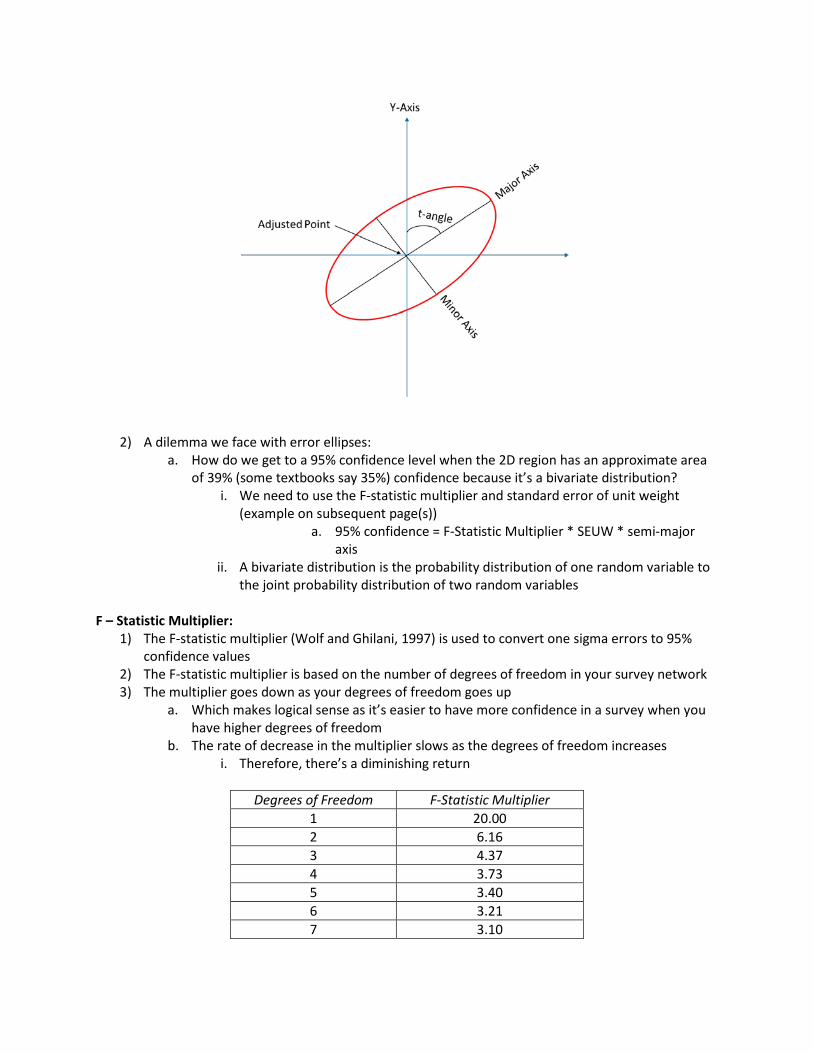
2) A dilemma we face with error ellipses: a. How do we get to a 95% confidence level when the 2D region has an approximate area

of 39% (some textbooks say 35%) confidence because it’s a bivariate distribution? i. We need to use the F-statistic multiplier and standard error of unit weight

(example on subsequent page(s)) a. 95% confidence = F-Statistic Multiplier * SEUW * semi-major

axis ii. A bivariate distribution is the probability distribution of one random variable to

the joint probability distribution of two random variables F – Statistic Multiplier:

1) The F-statistic multiplier (Wolf and Ghilani, 1997) is used to convert one sigma errors to 95% confidence values

2) The F-statistic multiplier is based on the number of degrees of freedom in your survey network 3) The multiplier goes down as your degrees of freedom goes up

a. Which makes logical sense as it’s easier to have more confidence in a survey when you have higher degrees of freedom

b. The rate of decrease in the multiplier slows as the degrees of freedom increases i. Therefore, there’s a diminishing return

Degrees of Freedom F-Statistic Multiplier

1 20.00 2 6.16 3 4.37 4 3.73 5 3.40 6 3.21 7 3.10

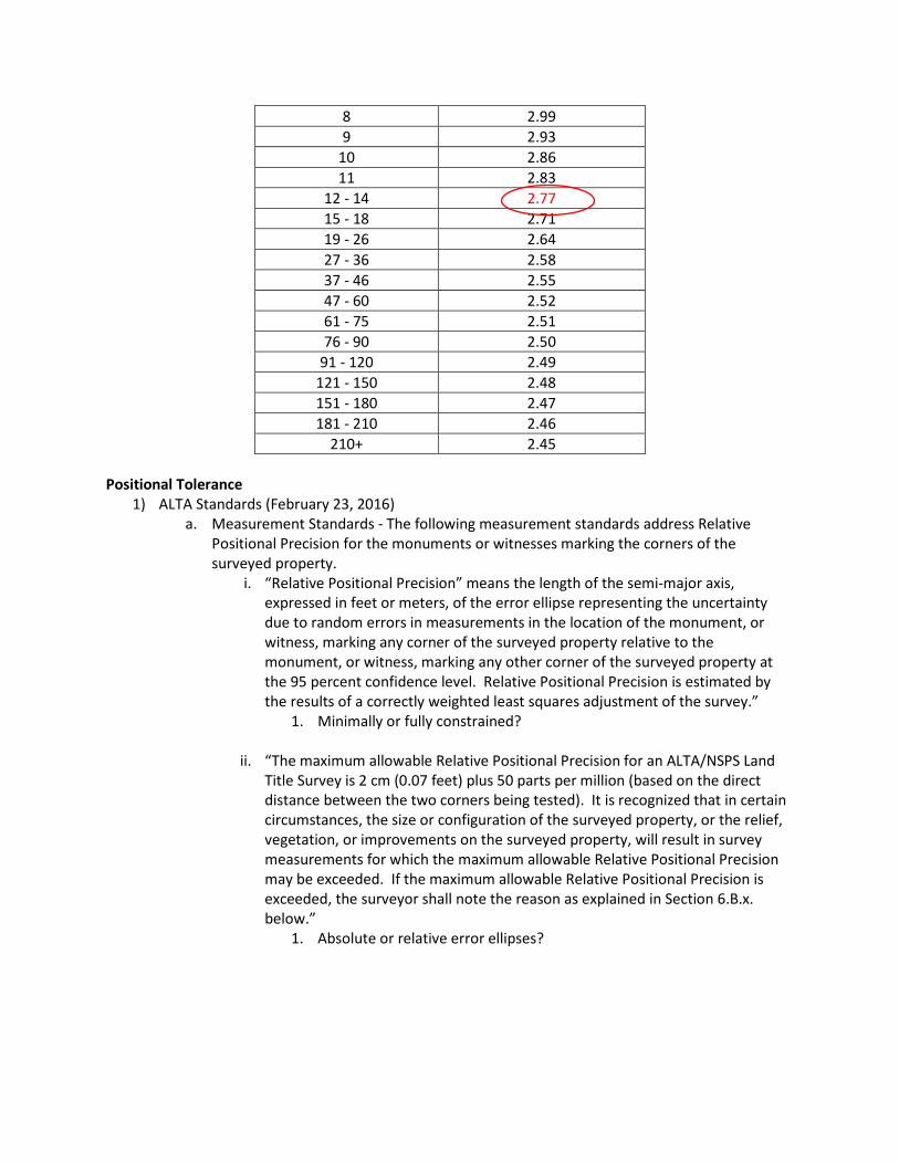
8 2.99 9 2.93

10 2.86 11 2.83

12 - 14 2.77 15 - 18 2.71 19 - 26 2.64 27 - 36 2.58 37 - 46 2.55 47 - 60 2.52 61 - 75 2.51 76 - 90 2.50

91 - 120 2.49 121 - 150 2.48 151 - 180 2.47 181 - 210 2.46

210+ 2.45

Positional Tolerance 1) ALTA Standards (February 23, 2016)

a. Measurement Standards - The following measurement standards address Relative Positional Precision for the monuments or witnesses marking the corners of the surveyed property.

i. “Relative Positional Precision” means the length of the semi-major axis, expressed in feet or meters, of the error ellipse representing the uncertainty due to random errors in measurements in the location of the monument, or witness, marking any corner of the surveyed property relative to the monument, or witness, marking any other corner of the surveyed property at the 95 percent confidence level. Relative Positional Precision is estimated by the results of a correctly weighted least squares adjustment of the survey.”

1. Minimally or fully constrained? ii. “The maximum allowable Relative Positional Precision for an ALTA/NSPS Land

Title Survey is 2 cm (0.07 feet) plus 50 parts per million (based on the direct distance between the two corners being tested). It is recognized that in certain circumstances, the size or configuration of the surveyed property, or the relief, vegetation, or improvements on the surveyed property, will result in survey measurements for which the maximum allowable Relative Positional Precision may be exceeded. If the maximum allowable Relative Positional Precision is exceeded, the surveyor shall note the reason as explained in Section 6.B.x. below.”

1. Absolute or relative error ellipses?

Numerical Example:

Scenario: b. 12 degrees of freedom (F-statistic multiplier = 2.77) c. A post-adjustment standard error of unit weight = 1.26 d. A one sigma semi-major axis of an error ellipse = 0.019 meters for an unknown station

located 6,000.000 meters from the nearest control point Solution:

a. 95% confidence = F-Statistic Multiplier * SEUW * semi-major axis i. Semi-major axis is at one sigma

b. 95% confidence = 2.77 * 1.26 * 0.019m = 0.066 m i. 0.066m is the semi-major axis at 95% confidence

1. Estimated positional error c. Allowable positional tolerance = constant + (ppm value ÷ 1,000,000)*distance

Positional tolerance standard: 0.010m + 10ppm Positional tolerance = 0.010m + (10 ÷ 1,000,000)*6,000.000m = 0.070m

d. Since the positional error at 95% confidence, 0.066m is less than the positional tolerance, 0.070m, the station passes by 0.004 meters

Chapter VII Basic Error Propagation, Error Estimation and Weighting

One of the main functions that any surveyor is tasked with is being an expert in measurement science, and part of this is understanding how errors propagate. This subject has wide application to all aspects of Geomatics (Construction Layout, Photogrammetry, LiDAR, Hydrographic Surveying, Boundary Surveying, Structural Deformation Monitoring, etc.), but we’ll focus on its general applicability and its use in least squares analysis herein. Generally error propagation is taught using partial derivatives from calculus, but unfortunately most forget this type of math after they leave school. However, every surveyor is quite good at algebra and trigonometry, therefore, it’s with this in mind that it’ll be reviewed from an algebraic approach in this chapter. While not all of the statistical definitions reviewed earlier in the course will be used herein, many will. Therefore, it’s vital that the reader be comfortable with all of those definitions before embarking on this portion of the course. Dr. Charles Ghilani wrote “Unknown values are often determined indirectly by making direct measurements of other quantities which are functionally related to the desired unknowns, then the unknowns are computed”. We see this in computing coordinates from angles and distances; obtaining station elevations from rod readings in differential leveling; etc. All directly measured quantities contain errors; therefore, any value computed from them contain errors as well. This process of moving errors forward is the topic of this section of the course, error propagation. In this discussion it’s assumed that only random errors are being propagated during the procedure, and that all systematic errors have been removed prior to the error propagation taking place. By analyzing how errors propagate, a general expression can be developed for the propagation of random errors through any function. This expression is generally expressed in the form of partial derivatives, but for this course we’ll take a look at how this process can be performed using basic algebra. This algebraic process can be most easily understood by breaking it down into the following steps and then illustrating the process with a few basic examples:

1) Calculate the quantity as if there’s no error 2) Calculate the quantity after adding the error estimate to the first measurement

a. Subtract this value from the one derived in step one 3) Calculate the quantity after adding the error estimate to the second measurement (the first

measurement should no longer have the error estimate added) a. Subtract this value from the one derived in step one

4) Repeat this process until each value and its corresponding error estimates have been used 5) Calculate the total estimated error by taking the square root of the sum of the squares

a. Basic equation for propagating error

i. √(eX12 + ex2

2 + … + exn2)

1. eX1 = estimated error in measurement one 2. eX2 = estimated error in measurement two 3. eXn = estimated error in measurement n

Let’s work through a few basic examples and tie some things together:

1) Basic example using measured distances with corresponding error estimates: a. 100.00’ ±0.01’ b. 200.00’ ±0.02’ c. 300.00’ ±0.03’

i. Total distance is 600.00’ with an estimates error of: 1. √(0.012 + 0.022 + 0.032) = ±0.04’

a. Measurement and estimated error reported = 600.00’ ±0.04’ 2) A rectangle measures 100.00’ ±0.05’ by 250.00’ ±0.09’, what is the area and its corresponding

error estimate? a. (100.00’)(250.00’) = 25,000 ft2 (without error) b. (100.00’ + 0.05’)(250.00’) = 25,012.5 ft2 (estimated error added to first measurement)

i. 25,000 ft2 - 25,012.5 ft2 = -12.5 ft2 (subtraction of value b from a) c. (100.00’)(250.00’ + 0.09’) = 25,009 ft2 (estimated error added to second measurement)

i. 25,000 ft2 - 25,009 ft2 = -9 ft2 (subtraction of value c from a) d. Propagate the total error by taking the square root of the sum of the squares

1. √(12.52 + 92) = ±15.4 ft2 a. You can just use the absolute value since the negatives will

become positives after they’re squared e. While the area equals 25,000 ft2, it should be recognized the area contains an estimated

error of ±15.4 ft2 3) A rectangular tank measures 40.00’ ±0.05’ x 20.00’ ±0.03’ x 10.00’ ±0.02’, determine the volume

and the estimated error. a. (40.00’)(20.00’)(10.00’) = 8,000 ft3 (without error) b. (40.00’ + 0.05’)(20.00’)(10.00’) = 8,010 ft3 (estimated error added to first measurement)

i. 8,000 ft3 – 8,010 ft3 = -10 ft3 (subtraction of value b from a) c. (40.00’)(20.00’ + 0.03’)(10.00’) = 8,012 ft3 (estimated error added to second

measurement) i. 8,000 ft3 – 8,012 ft3 = -12 ft3 (subtraction of value c from a)

d. (40.00’)(20.00’)(10.00’ + 0.02’) = 8,016 ft3 (estimated error added to third measurement)

i. 8,000 ft3 – 8,010 ft3 = -16 ft3 (subtraction of value d from a) e. Propagate the total error by taking the square root of the sum of the squares

i. √(102 + 122 +162) = ±22.4 ft3 f. While the volume equals 8,000 ft3, we need to acknowledged that the volume contains

an estimated error of ±22.4 ft3 4) Given point B has been set with respect to A along an azimuth of 40° ±30” and a distance of

100.00m ±2cm, what is the estimated error in position B with respect to A? a. This can be solved exactly like the examples above, but let’s introduce a shortcut that

works quite well: i. The shortcut is predicated on recognizing the following:

1. The estimated error in distance is along the line 2. The estimated error in azimuth (angle) is perpendicular to the line

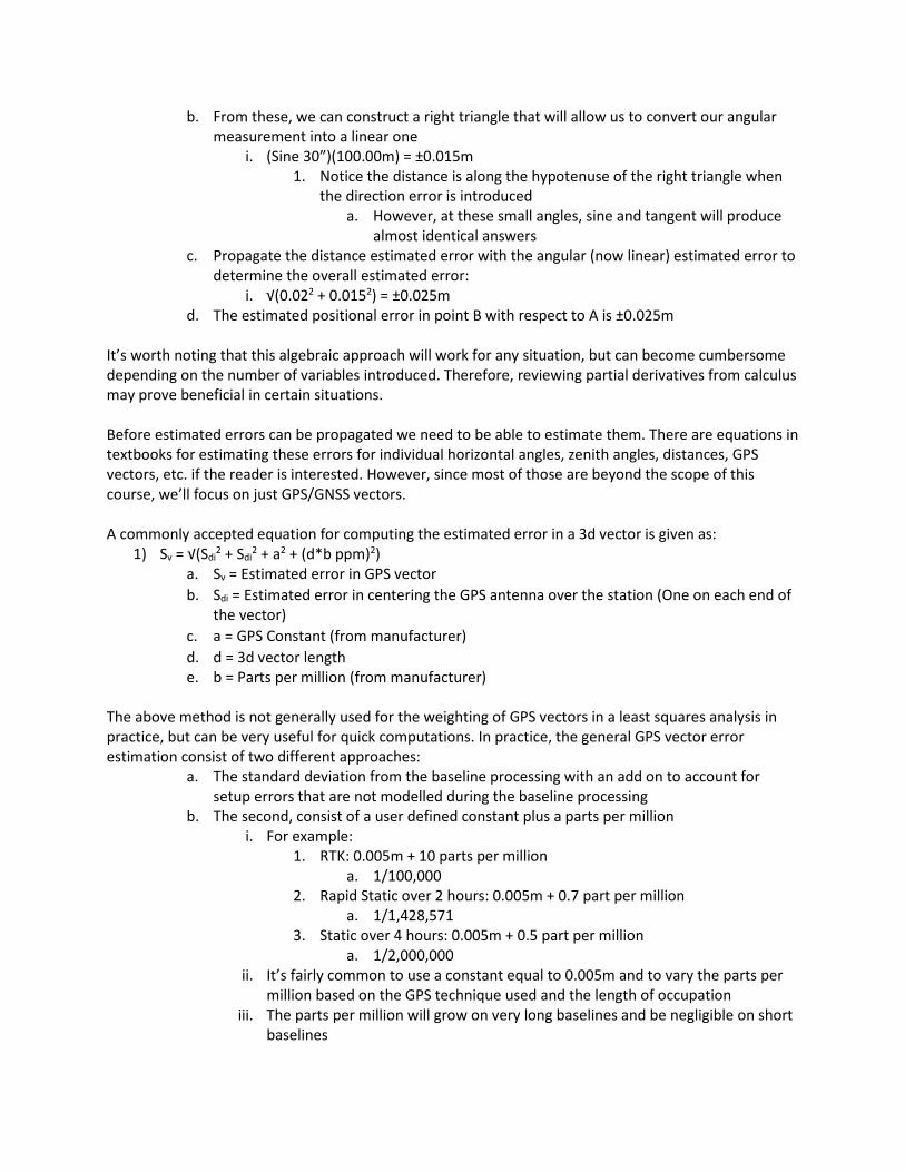
b. From these, we can construct a right triangle that will allow us to convert our angular measurement into a linear one

i. (Sine 30”)(100.00m) = ±0.015m 1. Notice the distance is along the hypotenuse of the right triangle when

the direction error is introduced a. However, at these small angles, sine and tangent will produce

almost identical answers c. Propagate the distance estimated error with the angular (now linear) estimated error to

determine the overall estimated error: i. √(0.022 + 0.0152) = ±0.025m

d. The estimated positional error in point B with respect to A is ±0.025m It’s worth noting that this algebraic approach will work for any situation, but can become cumbersome depending on the number of variables introduced. Therefore, reviewing partial derivatives from calculus may prove beneficial in certain situations. Before estimated errors can be propagated we need to be able to estimate them. There are equations in textbooks for estimating these errors for individual horizontal angles, zenith angles, distances, GPS vectors, etc. if the reader is interested. However, since most of those are beyond the scope of this course, we’ll focus on just GPS/GNSS vectors. A commonly accepted equation for computing the estimated error in a 3d vector is given as:

1) Sv = √(Sdi2 + Sdi

2 + a2 + (d*b ppm)2) a. Sv = Estimated error in GPS vector b. Sdi = Estimated error in centering the GPS antenna over the station (One on each end of

the vector) c. a = GPS Constant (from manufacturer) d. d = 3d vector length e. b = Parts per million (from manufacturer)

The above method is not generally used for the weighting of GPS vectors in a least squares analysis in practice, but can be very useful for quick computations. In practice, the general GPS vector error estimation consist of two different approaches:

a. The standard deviation from the baseline processing with an add on to account for setup errors that are not modelled during the baseline processing

b. The second, consist of a user defined constant plus a parts per million i. For example:

1. RTK: 0.005m + 10 parts per million a. 1/100,000

2. Rapid Static over 2 hours: 0.005m + 0.7 part per million a. 1/1,428,571

3. Static over 4 hours: 0.005m + 0.5 part per million a. 1/2,000,000

ii. It’s fairly common to use a constant equal to 0.005m and to vary the parts per million based on the GPS technique used and the length of occupation

iii. The parts per million will grow on very long baselines and be negligible on short baselines

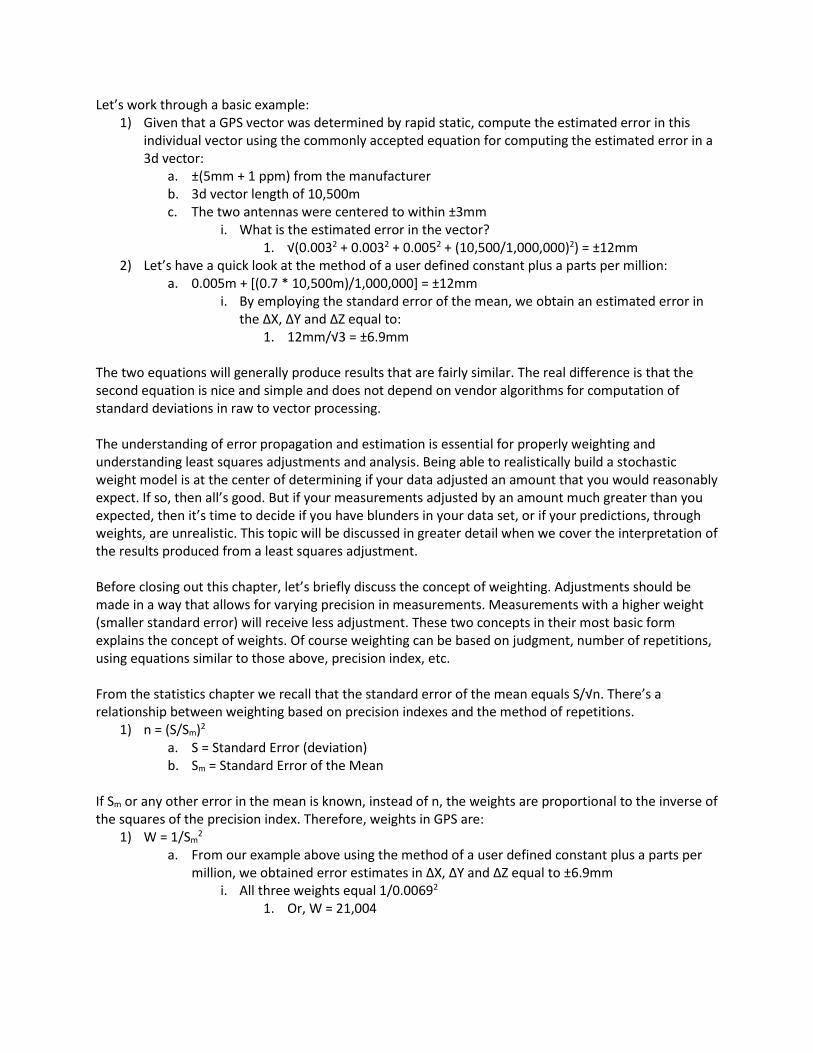
Let’s work through a basic example: 1) Given that a GPS vector was determined by rapid static, compute the estimated error in this

individual vector using the commonly accepted equation for computing the estimated error in a 3d vector:

a. ±(5mm + 1 ppm) from the manufacturer b. 3d vector length of 10,500m c. The two antennas were centered to within ±3mm

i. What is the estimated error in the vector? 1. √(0.0032 + 0.0032 + 0.0052 + (10,500/1,000,000)2) = ±12mm

2) Let’s have a quick look at the method of a user defined constant plus a parts per million: a. 0.005m + [(0.7 * 10,500m)/1,000,000] = ±12mm

i. By employing the standard error of the mean, we obtain an estimated error in the ΔX, ΔY and ΔZ equal to:

1. 12mm/√3 = ±6.9mm The two equations will generally produce results that are fairly similar. The real difference is that the second equation is nice and simple and does not depend on vendor algorithms for computation of standard deviations in raw to vector processing. The understanding of error propagation and estimation is essential for properly weighting and understanding least squares adjustments and analysis. Being able to realistically build a stochastic weight model is at the center of determining if your data adjusted an amount that you would reasonably expect. If so, then all’s good. But if your measurements adjusted by an amount much greater than you expected, then it’s time to decide if you have blunders in your data set, or if your predictions, through weights, are unrealistic. This topic will be discussed in greater detail when we cover the interpretation of the results produced from a least squares adjustment. Before closing out this chapter, let’s briefly discuss the concept of weighting. Adjustments should be made in a way that allows for varying precision in measurements. Measurements with a higher weight (smaller standard error) will receive less adjustment. These two concepts in their most basic form explains the concept of weights. Of course weighting can be based on judgment, number of repetitions, using equations similar to those above, precision index, etc. From the statistics chapter we recall that the standard error of the mean equals S/√n. There’s a relationship between weighting based on precision indexes and the method of repetitions.

1) n = (S/Sm)2 a. S = Standard Error (deviation) b. Sm = Standard Error of the Mean

If Sm or any other error in the mean is known, instead of n, the weights are proportional to the inverse of the squares of the precision index. Therefore, weights in GPS are:

1) W = 1/Sm2

a. From our example above using the method of a user defined constant plus a parts per million, we obtained error estimates in ΔX, ΔY and ΔZ equal to ±6.9mm

i. All three weights equal 1/0.00692 1. Or, W = 21,004

Chapter VIII Basic Concepts of Least Squares

At this juncture of the course, it’s time to cover the “dreaded least squares adjustment”. The interesting thing is, when dealing with GPS ECEF vector (coordinate) differences, it’s pretty straightforward. So for most taking this course, it’ll be a breeze. We’re going to cover this from two different approaches. First, we’ll review a theoretical approach using calculus (partial derivatives), going through it step by step; and then, we’ll review an applied approach where we’ll use prototype observation equations and matrix algebra. Theoretical Calculus Approach to Least Squares Scenario: Since GPS vectors are linear, that is a ΔX, ΔY and ΔZ, we’ll work through an example that involves coordinate pairs and fitting a best fit line, which is also linear. So let’s best fit a straight line through the following two-dimensional Cartesian coordinates (4 points, in x,y form) using a linear regression:

(3.00, 4.50) (4.25, 4.25) (5.50, 5.50) (8.00, 5.50)

Recall from geometry that the equation of a straight line is y = mx + b, and that it takes two sets of coordinates to define said line. Since we have four sets of coordinates it means that we have two degrees of freedom, and with degrees of freedom we have residuals (denoted as v). The concept of a least squares adjustment is predicated upon the concept of the most probable value is the one that renders the sum of the squares of the residuals to a minimum. We’ll review this concept in greater detail as we work through this example. Since there will be residuals, and we need to render the sum of the squares to a minimum, we need to add a residual to our standard equation:

v + y = mx + b or v = mx + b – y The first step in solving this scenario is to determine which form of the equation we want to use. We can use either one, but it’s easiest if we go ahead and isolate the residual on the left hand side and have everything else on the right hand side, so we’ll use the form: v = mx + b - y. Next, we’ll substitute in the x,y coordinate pairs (above) and form four different equations, again with residual on the left hand side isolated, and everything else on the right hand side:

v1 = 3.00m + b – 4.50 v2 = 4.25m + b – 4.25

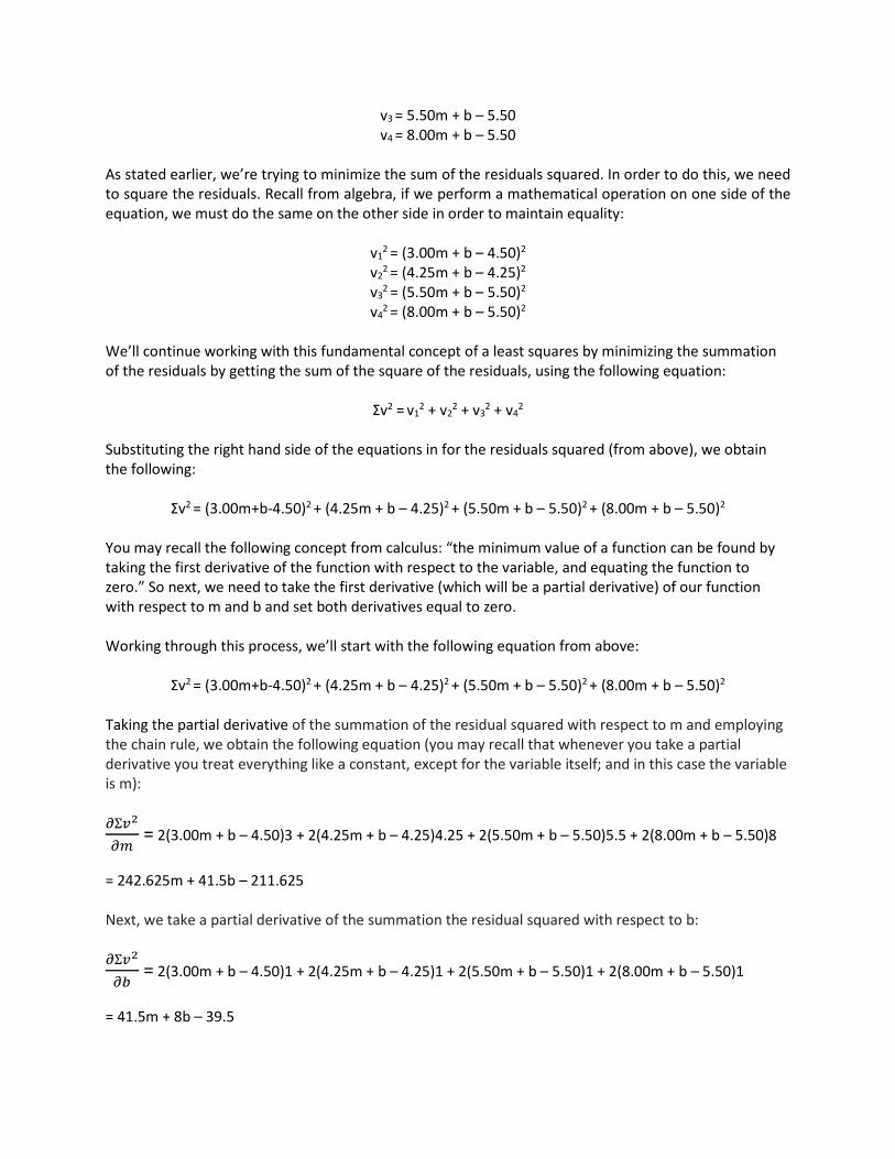
v3 = 5.50m + b – 5.50 v4 = 8.00m + b – 5.50

As stated earlier, we’re trying to minimize the sum of the residuals squared. In order to do this, we need to square the residuals. Recall from algebra, if we perform a mathematical operation on one side of the equation, we must do the same on the other side in order to maintain equality:

v12 = (3.00m + b – 4.50)2

v22 = (4.25m + b – 4.25)2

v32 = (5.50m + b – 5.50)2

v42 = (8.00m + b – 5.50)2

We’ll continue working with this fundamental concept of a least squares by minimizing the summation of the residuals by getting the sum of the square of the residuals, using the following equation:

Σv2 = v1

2 + v22 + v3

2 + v42

Substituting the right hand side of the equations in for the residuals squared (from above), we obtain the following:

Σv2 = (3.00m+b-4.50)2 + (4.25m + b – 4.25)2 + (5.50m + b – 5.50)2 + (8.00m + b – 5.50)2

You may recall the following concept from calculus: “the minimum value of a function can be found by taking the first derivative of the function with respect to the variable, and equating the function to zero.” So next, we need to take the first derivative (which will be a partial derivative) of our function with respect to m and b and set both derivatives equal to zero. Working through this process, we’ll start with the following equation from above:

Σv2 = (3.00m+b-4.50)2 + (4.25m + b – 4.25)2 + (5.50m + b – 5.50)2 + (8.00m + b – 5.50)2

Taking the partial derivative of the summation of the residual squared with respect to m and employing the chain rule, we obtain the following equation (you may recall that whenever you take a partial derivative you treat everything like a constant, except for the variable itself; and in this case the variable is m): 𝜕𝜕Ʃ𝑣𝑣2

𝜕𝜕𝜕𝜕 = 2(3.00m + b – 4.50)3 + 2(4.25m + b – 4.25)4.25 + 2(5.50m + b – 5.50)5.5 + 2(8.00m + b – 5.50)8

= 242.625m + 41.5b – 211.625 Next, we take a partial derivative of the summation the residual squared with respect to b: 𝜕𝜕Ʃ𝑣𝑣2

𝜕𝜕𝜕𝜕 = 2(3.00m + b – 4.50)1 + 2(4.25m + b – 4.25)1 + 2(5.50m + b – 5.50)1 + 2(8.00m + b – 5.50)1

= 41.5m + 8b – 39.5

In order to obtain the equation that best fits a straight line through the four sets of coordinate pairs we began with, we take both of the equations derived from our partial derivatives, set them equal to zero, and solve them simultaneously:

242.625m + 41.5b – 211.625 = 0 41.5m + 8b – 39.5 = 0

When the computations are completed, we get a value for m (slope) and b (y intercept) as:

m = 0.246 and b = 3.663 Our final solution is, therefore, y = 0.246x + 3.663 Even though we’ve obtained the equation for our best fit line, we shouldn’t stop there. We need to calculate our residuals, as well. Referring back to the original equation, and our solved slope and y intercept: v = mx + b – y, and m = 0.246 and b = 3.663, we can solve for the residuals. Solving for residuals vx for the four unique sets of x,y coordinates:

v1 = (3.00) (0.246) + 3.663 – 4.50 => -0.099 v2 = (4.25) (0.246) + 3.663 – 4.25 => 0.456 v3 = (5.50) (0.246) + 3.663 – 5.50 => -0.484 v4 = (8.00) (0.246) + 3.663 – 5.50 => 0.131

By employing matrix algebra together with observation equations, we can save a lot of time and work, and get the same result. This approach will be explained a little later on. Adjustment Mathematical Models Used in Least Squares There are generally two forms of mathematical adjustment models used in least squares, conditional adjustment and parametric adjustment: Conditional Adjustment: In conditional adjustments, geometric conditions are enforced upon the observations and their residuals. The equations established in a conditional adjustment are called conditional equations.

Examples of Conditional Equation

1) (n-2)180˚. This is what the interior angles of any closed polygon must equal to; it’s a condition of a closed polygon.

2) The summation of latitudes and departures of any closed polygon must equal 0; this too, is a condition of a closed polygon.

The use of condition equations are considered an older method of least squares adjustment, therefore, it won’t cover it in this course. The more modern method, which we’ll cover herein, is the parametric adjustment.

In a parametric adjustment, equations are formed that relate measured quantities to their residual observational errors, and to independent and unknown parameters. To do this we create observation equations. Prototype Observation Equations There are many types of observation equations, however, in this chapter we’ll review just two of them: linear regression and GPS ECEF coordinate differences. When performing a least squares adjustment using matrix algebra, these prototype observation equations are a key component. 1) Observation equation for a linear regression: vyi + yi = mxi + b 2) GPS ECEF coordinate difference observation equation(s):

Coordinate difference from Station A to Station B (A-B) -XA = ΔXA-B – XB + vXA-B -YA = ΔYA-B – YB + vYA-B -ZA = ΔZA-B – ZB + vZA-B

As one can see, for GPS there are three observation equations since it’s a 3D, ECEF coordinate system. Recall that in carrier phase, we really compute the coordinate differences, so our adjustment is designed to adjust these differences.

Matrix Equations – Equal Weight & Weighted Observation Equations We’ve been working our way through some background information that’s necessary to properly perform least squares adjustments using matrix algebra. We’ve reviewed prototype observation equations and now we’ll review the specific matrix form for solutions. Since this course is focused on applied approaches, we won’t go into detail on the theoretical formulation of the matrix normal equations. Instead they’ll be presented in the appropriate form for use in the adjustment. Equal Weight Case: The first matrix form that we’ll review is for an equal weight case, this is where your weights would all be 1. The equation is: ATAX = ATL Here, the A matrix is the coefficient matrix; the X matrix is the unknowns; and the L matrix is what’s on the right hand side of the equal sign. We need to, however, rearrange the initial equation to get X by itself on the left hand side since this is what we are solving for: X = (ATA)-1ATL

For computing residuals, we’ll use the following matric equation: v = AX - L

This may look familiar since it’s the same formula we used in the matrix algebra chapter when we solved for the unknowns. Weighted Case: One of the biggest advantages of using least squares is being able to weight your observations realistically in accordance to the field conditions, and the techniques and equipment used. Therefore, most of the time when talking about least squares, we’re talking about a weighted case.

In order to discuss a weighted least squares adjustment from a matrix perspective, we need to introduce what we’ll call a W matrix, which will be the weights of the observations. Recall that our equal weight case was ATAX = ATL. As you can see, to make this applicable for a weighted case, we needed to multiply through (introducing to both sides of the equation) the weight matrix, W: ATWAX = ATWL

Isolating our X matrix on the left hand side, we get: X = (ATWA)-1ATWL This will solve for the unknown X values and give us the most probably values, which is our least squares adjustment. Finally, our residuals will still be computed using: v = AX – L Matrix Equations – Selected Statistical Indicators Since we’re using matrix algebra to perform our least squares adjustments, it’s very helpful to be able to compute important statistical indicators that are used in the analysis of the adjustments. The first one that we’ll take a look at is the standard error of unit weight for a weighted network. Standard Error of Unit Weight – Weighted Network, denoted by S0:

DFWvvS

T

O =

Recall that the v matrix is our residual matrix, the W matrix is the weight matrix, and DF is for degrees of freedom. Once the standard error of unit weight has been computed, the estimated standard deviation for any unknowns that were computed from the system of weighted observation equations will need to be solved. However, before getting into the specifics of how this is done, we need to introduce the covariance matrix. In matrix notation it’s written as: N-1 = (ATWA)-1 What we’re wanting to use are the terms from the main diagonal of the covariance matrix, designated as Qxx. Once these values are extracted, we can move forward with computing the estimated error of each individual measurement by employing the following equation:

XXOi QSS = Where Si is the estimated error, SO is the standard error of unit weight and QXX is each diagonal term from the covariance matrix. Please note that these are at a 68% confidence level.

Hopefully by working through our previous linear regression example using matrix algebra, we can tie these concepts together.

Least Squares using Matrix Algebra – Example

Coordinates, in x,y format are: (3.00, 4.50); (4.25, 4.25); (5.50, 5.50); and (8.00, 5.50) Our prototype equation for a linear regression is: vyi + yi = mxi + b; therefore, our four corresponding observation equations are:

v1 + 4.50 = 3.00m + b v2 + 4.25 = 4.25m + b v3 + 5.50 = 5.50m + b v4 + 5.50 = 8.00m + b

Formulating our matrices in accordance with the aforementioned, we obtain:

𝑣𝑣 = �

𝑣𝑣1𝑣𝑣2𝑣𝑣3𝑣𝑣4

� 𝐿𝐿 = �

4.54.255.505.50

� 𝐴𝐴 = �

3.00 14.25 15.50 18.00 1

� 𝑋𝑋 = �𝑚𝑚𝑏𝑏 �

The matrix equation that we’ll use is for an equal wait case. X = (ATA)-1 ATL and v = AX – L

X = �0.2463.663� = 𝑚𝑚

𝑏𝑏 v = �

−0.0990.456

−0.4840.131

�

Now you’ll notice that when we write the equation, our solution for the best fit line is: y = 0.246x + 3.663 This matches the solution that we obtained using calculus at the beginning of the chapter and hopefully you can see it is a much easier and very computer friendly approach. Types of Adjustments In closing out this chapter, let’s briefly review the two types of adjustments that are possible from a control standpoint - a minimally constrained adjustment and a fully constrained adjustment. Minimally Constrained Adjustment: A minimally constrained adjustment holds the minimum amount of control required to solve the system of equations.

1) A level network would require one elevation held fixed to be able to determine the elevation of all the other stations, if everything is connected.

2) In a two dimensional network, we require one set of coordinates and one azimuth held fixed in order to calculate the coordinates of the other points.

3) A 3D terrestrial network requires one set of coordinates, one azimuth, and one elevation held fixed.

4) A GPS network requires one control station held fixed in x, y & z earth-centered earth fixed coordinates.

The important point about a minimally constrained adjustment is that it tests the validity of your work since it's not influenced by faulty control. Fully Constrained Adjustment: Finally, in a fully constrained adjustment all of your control is held fixed and you constrain your adjustment to those fixed values. In a fully constrained adjustment, if any of your control points have faulty values, it's going to show up in your statistical indicators when compared to those derived from your minimally constrained adjustment. In closing, both adjustments should always be performed. You should perform the minimally constrained adjustment first, to test the integrity of your work, and then perform the fully constrained adjustment to test the integrity of the control.

Chapter IX

Analysis of Adjustments

Congratulations, you’ve made it to the last chapter of the course. In this final chapter we’ll be covering different methods that can be employed to properly analyze the results from a least squares adjustment. We’ll begin by reviewing the basic underlying concepts. First, it’s important to point out that there's no cookie cutter process that can be used for all types of scenarios. One must exercise common sense, coupled with experience, in order to determine if you have a valid adjustment. From a statistical standpoint, you are analyzing the statistical indicators produced from the adjustment, as if your data set is normally distributed. If you have normally distributed data, there are certain laws that the data will obey:

1) Approximately 50% of your residuals should be positive and approximately 50% should be negative.

2) Approximately 68% of your normalized residuals, if weighted properly and no outliers exist, should be equal to or less than one.

3) If you have any normalized residuals greater than 3.0, they should be closely examined as potential outliers.

4) Finally, the standard error of unit weight is statistically evaluated using the Chi Squared Test. Recall that normalized residuals are an indication of your weighting for individual observations, and the standard error of unit weight is an indication of your weighting for a group of like observations and your entire network. Now, let's look at each one of our normally distributed data set points (above) in greater detail. We’ll begin with looking at the sign of our residuals. We have created a set of tables (on following pages) that contain our statistical indicators as an aid to our discussion. We’ll be using these during most of this chapter. Residuals As a review, a residual is the difference between your adjusted value and your measured or observed value. You are looking for approximately 50% of your residuals to be positive, and approximately 50% to be negative. If you have 90% negative and 10% positive, or vice-versa, you need to examine them because you have a potential problem with your data set (likely a systematic error exist).

GPS Vector Adjustment Data

From To Hor. Residuals

Ver. Residuals

3D Residuals

3D Error Estimate

Normalized Residual

TN26 PDH7

-0.0123 -0.0735 -0.0745 0.1015 0.7

TN22 PDH7 -0.0612 0.0800 -0.1007 0.2134 0.5

TN17 PDH7 0.0933 -0.2498 0.2667 0.2035 1.3

TN16 PDH7

-0.0187 -0.0209 -0.0280 0.0745 0.4

TN28 PDH7 0.0640 0.1932 0.2035 0.2813 0.7

TN23 PDH7 0.0278 0.1371 0.1399 0.1037 1.3 Approximately 50% positive and 50% negative Residual = Adjusted – Observed In our example, there are three negative and three positive for our horizontal residuals; so, this is a good first indicator that we have a valid adjustment. However, there are several other indicators that we need to examine before making our final conclusion. It's very important that all of our indicators are examined as a whole as this is the only way we can get a complete picture of our adjustment. Continuing with analysis of our residuals, we will now examine the vertical residuals circled in red. Like the horizontal, there are three negative and three positive ones; this too is a good sign. GPS Vector Adjustment Data

From To Hor. Residuals

Ver. Residuals

3D Residuals

3D Error Estimate

Normalized Residual

TN26 PDH7 -0.0123 -0.0735 -0.0745 0.1015 0.7

TN22 PDH7 -0.0612 0.0800 -0.1007 0.2134 0.5

TN17 PDH7 0.0933 -0.2498 0.2667 0.2035 1.3

TN16 PDH7 -0.0187 -0.0209 -0.0280 0.0745 0.4

TN28 PDH7 0.0640 0.1932 0.2035 0.2813 0.7

TN23 PDH7 0.0278 0.1371 0.1399 0.1037 1.3 Approximately 50% positive and 50% negative Residual = Adjusted - Observed

And finally, in terms of our residuals, let’s have a look at 3D residuals. Here too, we have three negative and three positive so this too is a good sign. It’s important that we also examine the size of the residuals. Are they approximately equal to what the equipment is spec’d at plus any add-ons for things such as centering error? Next, we’ll use normalized residuals to assist us with this task. GPS Vector Adjustment Data

From To Hor. Residuals

Ver. Residuals

3D Residuals

3D Error Estimate

Normalized Residual

TN26 PDH7 -0.0123 -0.0735 -0.0745 0.1015 0.7

TN22 PDH7 -0.0612 0.0800 -0.1007 0.2134 0.5

TN17 PDH7 0.0933 -0.2498 0.2667 0.2035 1.3

TN16 PDH7 -0.0187 -0.0209 -0.0280 0.0745 0.4

TN28 PDH7 0.0640 0.1932 0.2035 0.2813 0.7

TN23 PDH7 0.0278 0.1371 0.1399 0.1037 1.3 Approximately 50% positive and 50% negative 3D Residual = Adjusted 3D Vector – Observed 3D Vector Normalized Residuals According to normally distributed data set rules, we're expecting approximately 68% of our normalized residuals to be equal to or less than one. Recalling that normalized residual are also referred to as standardized residuals, snoop numbers, snoop values and the W test; and is equal to the absolute value of the residual divided by the error estimate. In the example below, we are analyzing the normalized residuals for our 3D residuals; although we can also examine them for horizontal and vertical. There are six 3D residuals, so we are expecting approximately four of them to be equal to or less than one. Since we have four, and none are equal to or greater than 3.0, this is a good sign. Remember that normalized residuals are an indication of our individual weighting of observations.

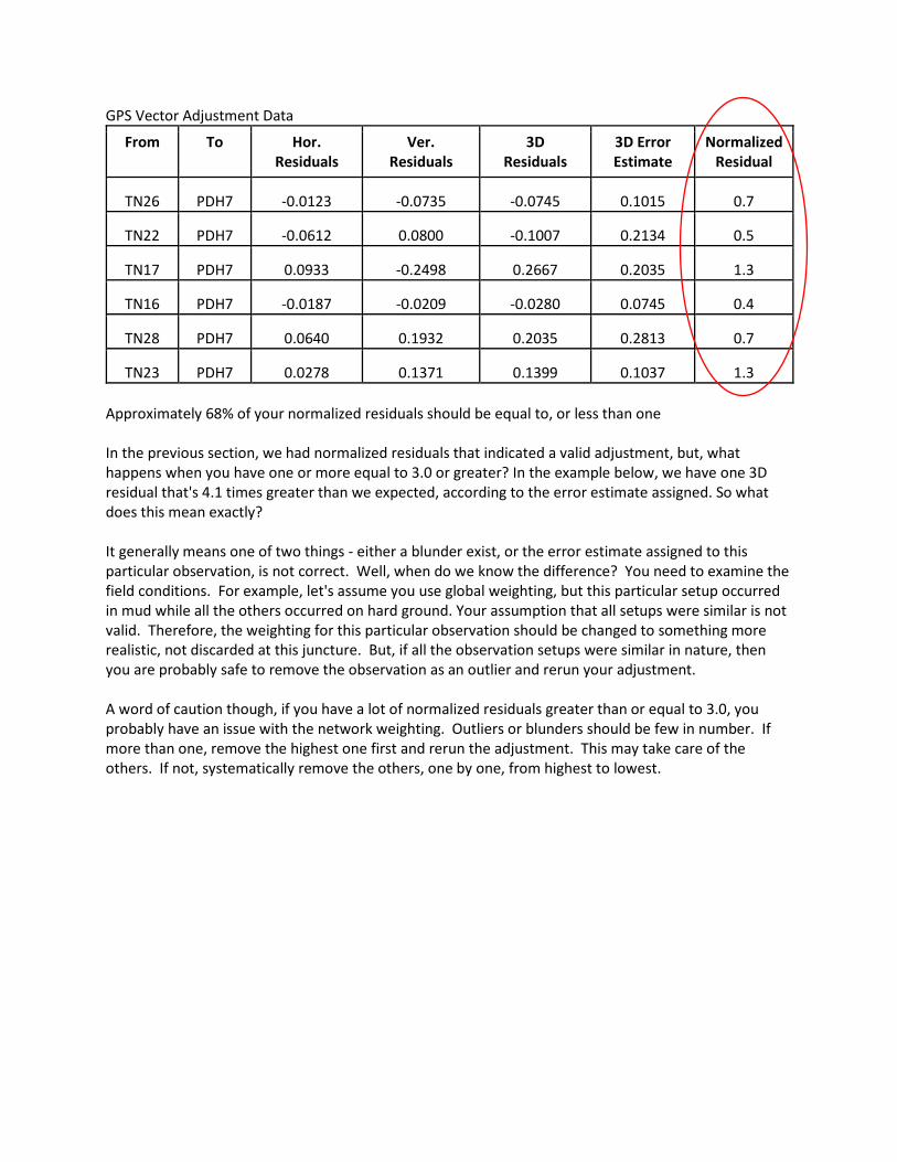
GPS Vector Adjustment Data

From To Hor. Residuals

Ver. Residuals

3D Residuals

3D Error Estimate

Normalized Residual

TN26 PDH7 -0.0123 -0.0735 -0.0745 0.1015 0.7

TN22 PDH7 -0.0612 0.0800 -0.1007 0.2134 0.5

TN17 PDH7 0.0933 -0.2498 0.2667 0.2035 1.3

TN16 PDH7 -0.0187 -0.0209 -0.0280 0.0745 0.4

TN28 PDH7 0.0640 0.1932 0.2035 0.2813 0.7

TN23 PDH7 0.0278 0.1371 0.1399 0.1037 1.3 Approximately 68% of your normalized residuals should be equal to, or less than one In the previous section, we had normalized residuals that indicated a valid adjustment, but, what happens when you have one or more equal to 3.0 or greater? In the example below, we have one 3D residual that's 4.1 times greater than we expected, according to the error estimate assigned. So what does this mean exactly? It generally means one of two things - either a blunder exist, or the error estimate assigned to this particular observation, is not correct. Well, when do we know the difference? You need to examine the field conditions. For example, let's assume you use global weighting, but this particular setup occurred in mud while all the others occurred on hard ground. Your assumption that all setups were similar is not valid. Therefore, the weighting for this particular observation should be changed to something more realistic, not discarded at this juncture. But, if all the observation setups were similar in nature, then you are probably safe to remove the observation as an outlier and rerun your adjustment. A word of caution though, if you have a lot of normalized residuals greater than or equal to 3.0, you probably have an issue with the network weighting. Outliers or blunders should be few in number. If more than one, remove the highest one first and rerun the adjustment. This may take care of the others. If not, systematically remove the others, one by one, from highest to lowest.

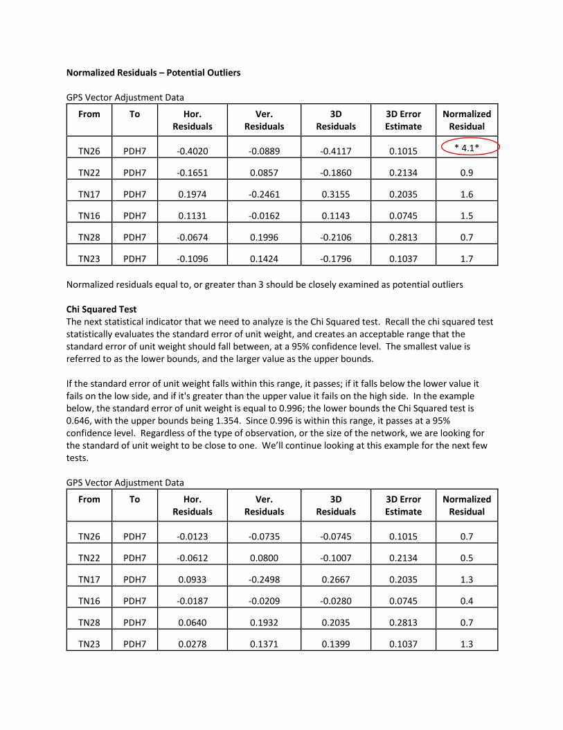
Normalized Residuals – Potential Outliers GPS Vector Adjustment Data

From To Hor. Residuals

Ver. Residuals

3D Residuals

3D Error Estimate

Normalized Residual

TN26 PDH7 -0.4020 -0.0889 -0.4117 0.1015 * 4.1*

TN22 PDH7 -0.1651 0.0857 -0.1860 0.2134 0.9

TN17 PDH7 0.1974 -0.2461 0.3155 0.2035 1.6

TN16 PDH7 0.1131 -0.0162 0.1143 0.0745 1.5

TN28 PDH7 -0.0674 0.1996 -0.2106 0.2813 0.7

TN23 PDH7 -0.1096 0.1424 -0.1796 0.1037 1.7 Normalized residuals equal to, or greater than 3 should be closely examined as potential outliers Chi Squared Test The next statistical indicator that we need to analyze is the Chi Squared test. Recall the chi squared test statistically evaluates the standard error of unit weight, and creates an acceptable range that the standard error of unit weight should fall between, at a 95% confidence level. The smallest value is referred to as the lower bounds, and the larger value as the upper bounds. If the standard error of unit weight falls within this range, it passes; if it falls below the lower value it fails on the low side, and if it's greater than the upper value it fails on the high side. In the example below, the standard error of unit weight is equal to 0.996; the lower bounds the Chi Squared test is 0.646, with the upper bounds being 1.354. Since 0.996 is within this range, it passes at a 95% confidence level. Regardless of the type of observation, or the size of the network, we are looking for the standard of unit weight to be close to one. We’ll continue looking at this example for the next few tests. GPS Vector Adjustment Data

From To Hor. Residuals

Ver. Residuals

3D Residuals

3D Error Estimate

Normalized Residual

TN26 PDH7 -0.0123 -0.0735 -0.0745 0.1015 0.7

TN22 PDH7 -0.0612 0.0800 -0.1007 0.2134 0.5

TN17 PDH7 0.0933 -0.2498 0.2667 0.2035 1.3

TN16 PDH7 -0.0187 -0.0209 -0.0280 0.0745 0.4

TN28 PDH7 0.0640 0.1932 0.2035 0.2813 0.7

TN23 PDH7 0.0278 0.1371 0.1399 0.1037 1.3

Standard Error of Unit Weight is 0.996 with 15 degrees of freedom Chi Squared Test on Analysis

0.646 < 0.996 < 1.354 (Low) (High)

Passes at the 5% Significance Level Chi Squared Test – Potential Outliers In the next example below, we have a normalized residual greater than 3.0 that’s causing the standard error of unit weight to exceed the upper bounds of the Chi Squared test. So, this particular normalized residual needs to be closely examined, and if it's a blunder it needs to be removed. Conversely, if the weighting is incorrect, the weighting needs to be corrected. When one of these remedies occurs, we’d expect to see the Chi Squared test pass. GPS Vector Adjustment Data

From To Hor. Residuals

Ver. Residuals

3D Residuals

3D Error Estimate

Normalized Residual

TN26 PDH7 -0.4020 -0.0889 -0.4117 0.1015

* 4.1*

TN22 PDH7 -0.1651 0.0857 -0.1860 0.2134 0.9

TN17 PDH7 0.1974 -0.2461 0.3155 0.2035 1.6

TN16 PDH7 0.1131 -0.0162 0.1143 0.0745 1.5

TN28 PDH7 -0.0674 0.1996 -0.2106 0.2813 0.7

TN23 PDH7 -0.1096 0.1424 -0.1796 0.1037 1.7

Standard Error of Unit Weight is 2.260 with 15 degrees of freedom Chi Squared Test on Analysis

0.646 < 2.260 < 1.354 (Low) (High)

Fails at the 5% Significance Level

Chi Squared Test – Weighting Too Pessimistic In the example below, we fail the Chi Squared test on the low side, and all of our normalized residuals are less than 1. This is an indication that we are too pessimistic in our network weighting, and that we did better work than we thought we were going to do. So in this example, we need to tighten up our weighting for the entire network. Now, failing on the low side is not that big of a deal because we did better work than we thought, however, we should strive to have our weighting correct. GPS Vector Adjustment Data

From To Hor. Residuals

Ver. Residuals

3D Residuals

3D Error Estimate

Normalized Residual

TN26 PDH7 -0.0123 -0.0732 -0.0743 0.6480 0.1

TN22 PDH7 -0.0616 0.0802 -0.1012 1.3938 0.1

TN17 PDH7 0.0934 -0.2495 0.2664 1.3290 0.2

TN16 PDH7 -0.0184 -0.0206 -0.0276 0.4678 0.1

TN28 PDH7 0.0639 0.1934 0.2037 1.8467 0.1

TN23 PDH7 0.0280 0.1373 0.1402 0.6634 0.2

Standard Error of Unit Weight is 0.154 with 15 degrees of freedom Chi Squared Test on Analysis

0.646 < 0.154 < 1.354 (Low) (High)

Fails at the 5% Significance Level Chi Squared Test – Weighting Too Optimistic In the example below, we fail the Chi Squared test on the high side. Since we have no potential outliers being flagged by our normalized residuals being equal to exceeding 3.0, this indicates that our weighting for the entire network is too optimistic. Here, we think we did better work than we actually did. This is a problem and it needs to be corrected. We need to loosen up our weighting and rerun the adjustment.

GPS Vector Adjustment Data

From To Hor. Residuals

Ver. Residuals

3D Residuals

3D Error Estimate

Normalized Residual

TN26 PDH7 -0.0122 -0.0738 -0.0748 0.0613 1.2

TN22 PDH7 -0.0609 0.0797 -0.1003 0.1264 0.8

TN17 PDH7 0.0933 -0.2501 0.2669 0.1209

2.2

TN16 PDH7 -0.0190 -0.0212 -0.0285 0.0456 0.6

TN28 PDH7 0.0640 0.1929 0.2032 0.1661 1.2

TN23 PDH7 0.0277 0.1368 0.1395 0.0625 2.2

Standard Error of Unit Weight is 1.665 with 15 degrees of freedom Chi Squared Test on Analysis

0.646 < 1.665 < 1.354 (Low) (High)

Fails at the 5% Significance Level Estimated Error in the Adjusted Values In this section, we need to review the estimated error in our adjusted value. This task is very important in being able to determine if our positional error is less than our positional tolerance standard. Below, we have the adjusted latitude, longitude and ellipsoidal height for station PDH7 and the estimated errors in each of these components in meters, at a 95% confidence level. GPS Vector Adjustment Data

Station Latitude Longitude Height

SD (meters) SD (meters) SD (meters)

PDH7 35°43’17.64335” 84°43’41.37707” 209.0412

0.0252 0.0252 0.0252

Estimated errors in the adjusted position of PDH7 at a 95% confidence:

Horizontal: ±0.0252m Vertical: ±0.0252m

The reason σx = σy = σz is because the vector components were treated as being uncorrelated. The question to be answered is, do these values meet State or project specifications? If so, great! But if not, we may need to add additional observations in order to increase our degrees of freedom. In closing out this chapter, it’s important to stress that no adjustment can turn bad data into good data.

I would like to acknowledge and thank the following individuals for their teachings and writings. Without them, this course would not have been possible. Ben Buckner, PhD Marian Clark, PhD David Doyle Ahmed El Rabbany, PhD Charles Ghilani, PhD Ray Hintz, PhD Jeff Hurn Huibert-Jan Lekkerkerk Martin McClinton, PhD Jan Van Sickle James R. Smith Herbert Stoughton, PhD